5. Perfect competition analysis

Contents perfect competition characteristics firm´s equilibrium in short run firm´s short run supply curve short industry supply curve firm´s equilibrium in long run long industry supply curve perfect competition efficiency impact of price regulation

Characteristics of perfect competition environment...

many buyers and many sellers on each market no one is strong enough to influence the price or industry

output all goods are homogenous no barriers to enter or leave the industry all producers and consumers are perfectly informed of price

and quantity on each market firms endeavour to maximize their profits, consumers

endeavour to maximize their total utilities

...and facts implying

firm is a price taker – equilibrium price is set by the market equilibrium

each firm has a neglectable market share firm´s individual demand is horizontal at the level of equilibrium

price marginal and average revenue functions equal to the individual

demand function

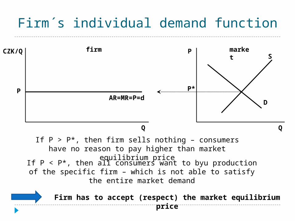
Firm´s individual demand function

Q

CZK/Q

AR=MR=P=d

marketS

D

Q

Pfirm

P*

If P > P*, then firm sells nothing – consumers have no reason to pay higher than market equilibrium price

If P < P*, then all consumers want to byu production of the specific firm – which is not able to satisfy the entire market demand

Firm has to accept (respect) the market equilibrium price

P

Firm´s short run equilibrium output

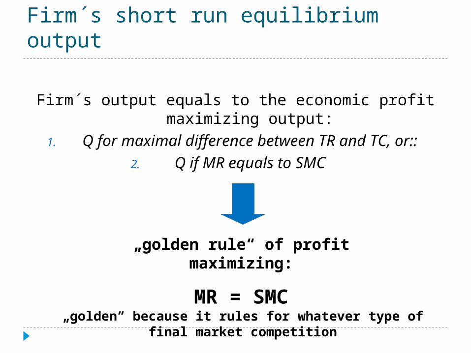
Firm´s output equals to the economic profit maximizing output:1. Q for maximal difference between TR and TC, or::

2. Q if MR equals to SMC

„golden rule“ of profit maximizing:

MR = SMC

„golden“ because it rules for whatever type of final market competition

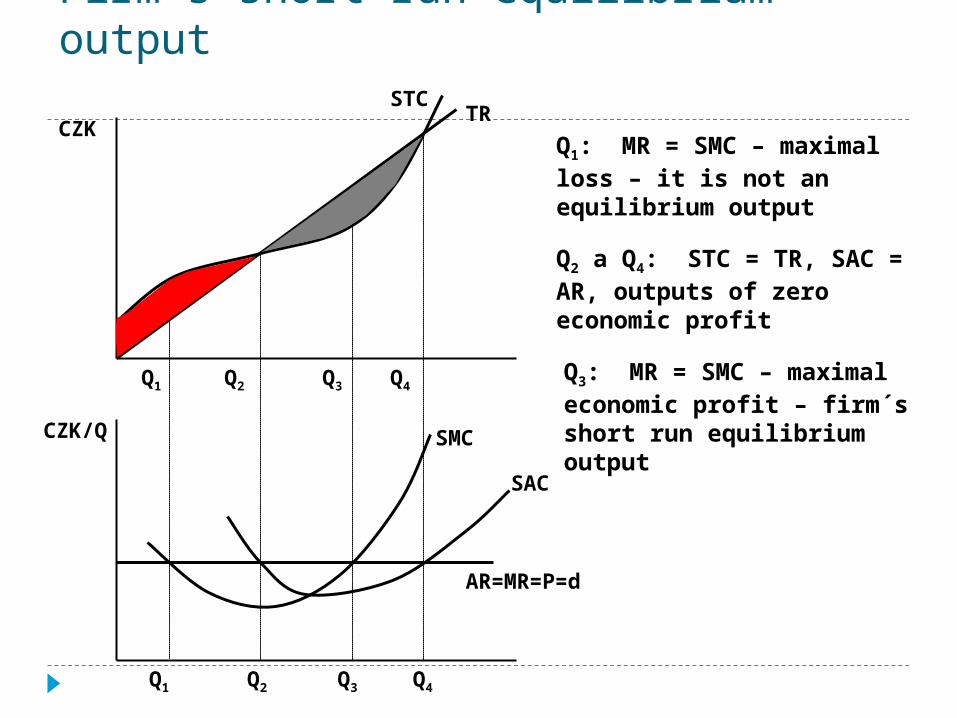
Firm´s short run equilibrium output

Q1

Q1

Q2

Q2

Q3

Q3

Q4

Q4

CZK/Q

CZK

SMC

SAC

AR=MR=P=d

STCTR

Q1: MR = SMC – maximal loss – it is not an equilibrium output

Q2 a Q4: STC = TR, SAC = AR, outputs of zero economic profit

Q3: MR = SMC – maximal economic profit – firm´s short run equilibrium output

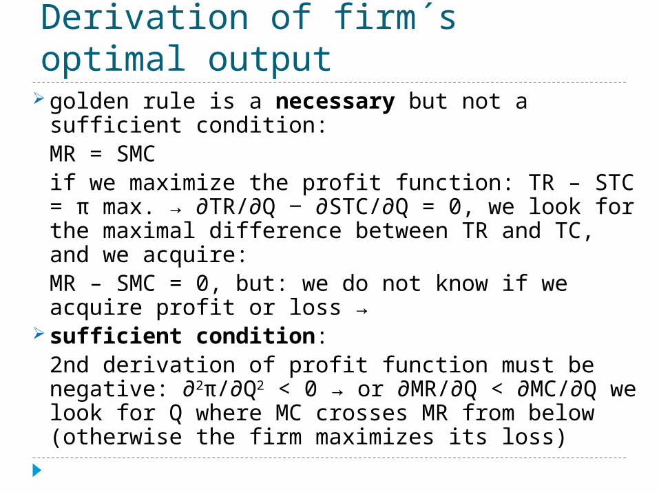
Derivation of firm´s optimal output golden rule is a necessary but not a sufficient condition:

MR = SMCif we maximize the profit function: TR – STC = π max. → ∂TR/∂Q ‒ ∂STC/∂Q = 0, we look for the maximal difference between TR and TC, and we acquire:MR – SMC = 0, but: we do not know if we acquire profit or loss →

sufficient condition:2nd derivation of profit function must be negative: ∂2π/∂Q2 < 0 → or ∂MR/∂Q < ∂MC/∂Q we look for Q where MC crosses MR from below (otherwise the firm maximizes its loss)

Firm´s short run supply curve

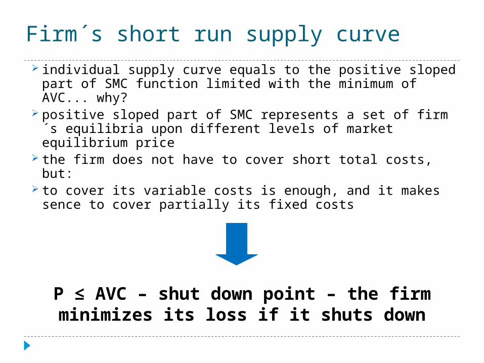
individual supply curve equals to the positive sloped part of SMC function limited with the minimum of AVC... why?

positive sloped part of SMC represents a set of firm´s equilibria upon different levels of market equilibrium price

the firm does not have to cover short total costs, but: to cover its variable costs is enough, and it makes sence to

cover partially its fixed costs

P ≤ AVC – shut down point – the firm minimizes its loss if it shuts down

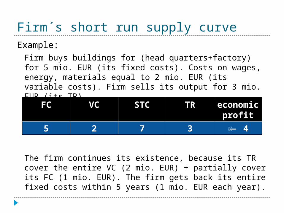
Example:Firm buys buildings for (head quarters+factory) for 5 mio. EUR (its fixed costs). Costs on wages, energy, materials equal to 2 mio. EUR (its variable costs). Firm sells its output for 3 mio. EUR (its TR)

The firm continues its existence, because its TR cover the entire VC (2 mio. EUR) + partially cover its FC (1 mio. EUR). The firm gets back its entire fixed costs within 5 years (1 mio. EUR each year).

Firm´s short run supply curve

FC VC STC TR economic profit

5 2 7 3 ̶� 4

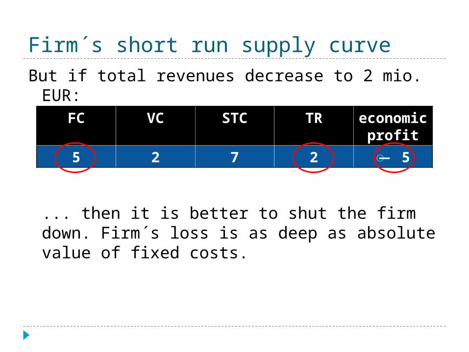
But if total revenues decrease to 2 mio. EUR:

... then it is better to shut the firm down. Firm´s loss is as deep as absolute value of fixed costs.

Firm´s short run supply curve

FC VC STC TR economic profit

5 2 7 2 ̶� 5

Firm´s short run supply curve

Q1Q2

CZK/Q SMC

SAC

AR=MR=P=d

AVC

AR'=MR'=P'=d'

S

D

D'

Q

P

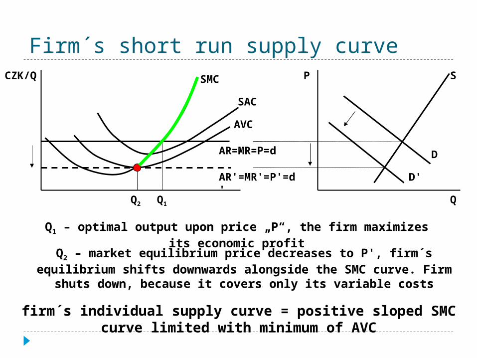
Q1 – optimal output upon price „P“, the firm maximizes its economic profit

Q2 – market equilibrium price decreases to P', firm´s equilibrium shifts downwards alongside the SMC curve. Firm shuts down, because it covers only its variable costs

firm´s individual supply curve = positive sloped SMC curve limited with minimum of AVC

Short industry supply curve – constant prices of inputs

CZK/Q

Q

MC1 MC2 SIS (∑MC)

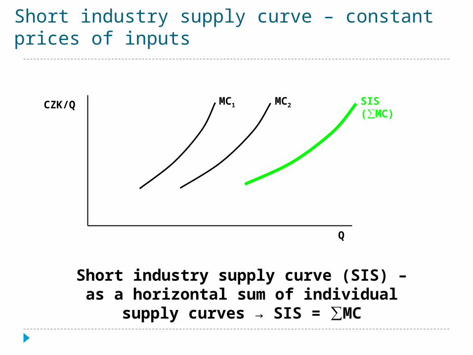
Short industry supply curve (SIS) – as a horizontal sum of individual supply curves → SIS = ∑MC

Short industry supply curve – increasing prices of inputs

CZK/Q

Q

MC' MC

SIS

P2

P1

Q1 Q2Q3

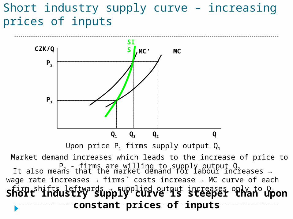
Upon price P1 firms supply output Q1

Market demand increases which leads to the increase of price to P2 - firms are willing to supply output Q2

It also means that the market demand for labour increases → wage rate increases → firms´ costs increase → MC curve of each firm shifts leftwards → supplied output increases only to Q3

Short industry supply curve is steeper than upon constant prices of inputs

Firm´s long run equilibrium output

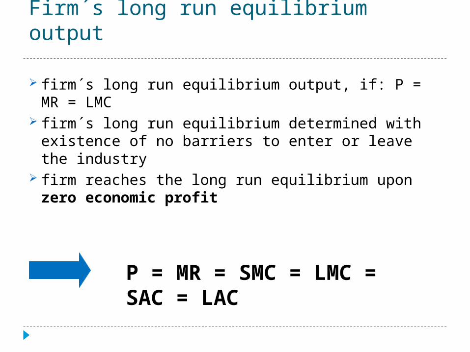
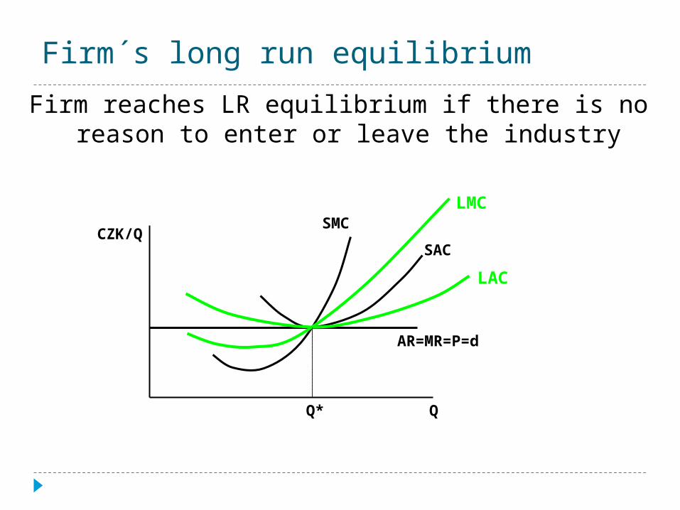
firm´s long run equilibrium output, if: P = MR = LMC firm´s long run equilibrium determined with existence of no

barriers to enter or leave the industry firm reaches the long run equilibrium upon zero economic

profit

P = MR = SMC = LMC = SAC = LAC

Firm´s long run equilibrium

Firm reaches LR equilibrium if there is no reason to enter or leave the industry

Q* Q

CZK/QSMC

SAC

AR=MR=P=d

LAC

LMC

Firm´s long run equilibrium

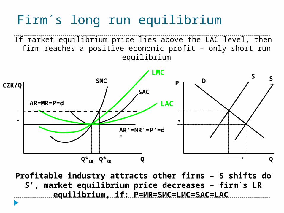
If market equilibrium price lies above the LAC level, then firm reaches a positive economic profit – only short run equilibrium

Q*LR Q

CZK/QSMC

SAC

AR'=MR'=P'=d'

LAC

LMC

Q*SR

S S'D

Profitable industry attracts other firms – S shifts do S'‚ market equilibrium price decreases – firm´s LR equilibrium, if: P=MR=SMC=LMC=SAC=LAC

AR=MR=P=d

Q

P

Firm´s long run equilibrium

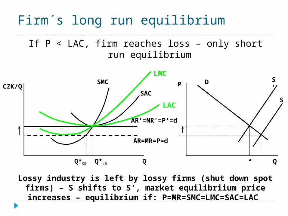
If P < LAC, firm reaches loss – only short run equilibrium

Q*LR Q

SMC

SAC

AR'=MR'=P'=d'

LAC

LMC

Q*SR

S

S'D

AR=MR=P=d

Q

PCZK/Q

Lossy industry is left by lossy firms (shut down spot firms) – S shifts to S'‚ market equilibriium price increases – equilibrium if: P=MR=SMC=LMC=SAC=LAC

Firm´s long run supply curve

Is this right?:

„Firm´s long run supply curve equals to the positive sloped part of LMC curve limited with the minimum LAC.“

Long industry supply curve

Industry supply = set of long run firms´equilibria = set of intersections of shifting demand curve and short industry supply

curves

LIS curve (Long Industry Supply)

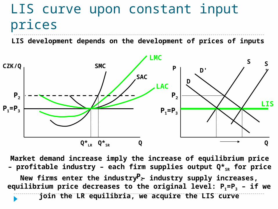
LIS curve upon constant input pricesLIS development depends on the development of prices of inputs

CZK/Q

Q*LR Q

SMC

SAC

LAC

LMC

Q*SR

S S'

D

Q

P D'

P1=P3 P1=P3

P2 P2

LIS

Market demand increase imply the increase of equilibrium price – profitable industry – each firm supplies output Q*SR for price P2

New firms enter the industry – industry supply increases, equilibrium price decreases to the original level: P1=P3 – if we join the LR equilibria, we acquire the LIS curve

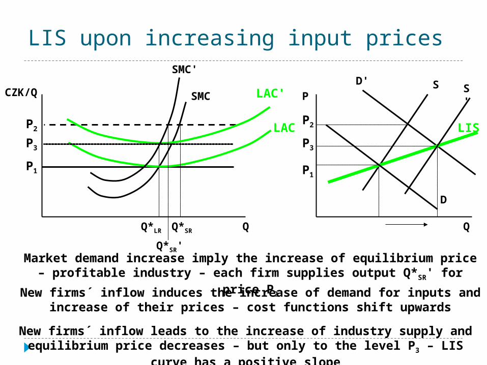
LIS upon increasing input prices

CZK/Q

Q*LR Q

SMC

LAC

Q*SR

S S'

D

Q

P

D'

P1 P1

P2P2 LIS

SMC'

LAC'

P3P3

Q*SR'

New firms´ inflow induces the increase of demand for inputs and increase of their prices – cost functions shift upwards

New firms´ inflow leads to the increase of industry supply and equilibrium price decreases – but only to the level P3 – LIS curve has a positive slope

Market demand increase imply the increase of equilibrium price – profitable industry – each firm supplies output Q*SR' for price P2

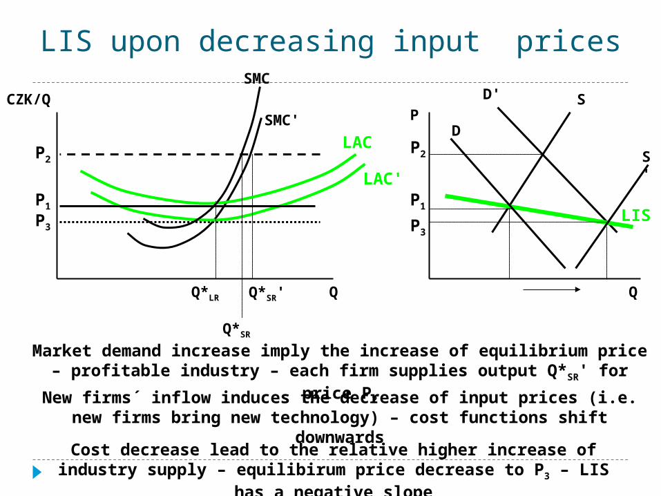
LIS upon decreasing input prices

Q*LR Q

SMC

LAC

Q*SR

S

S'

D

Q

P

D'

P1 P1

P2P2

LIS

SMC'

LAC'

P3P3

Q*SR'

CZK/Q

Cost decrease lead to the relative higher increase of industry supply – equilibirum price decrease to P3 – LIS has a negative slope

Market demand increase imply the increase of equilibrium price – profitable industry – each firm supplies output Q*SR' for price P2

New firms´ inflow induces the decrease of input prices (i.e. new firms bring new technology) – cost functions shift downwards

Perfect competition efficiency

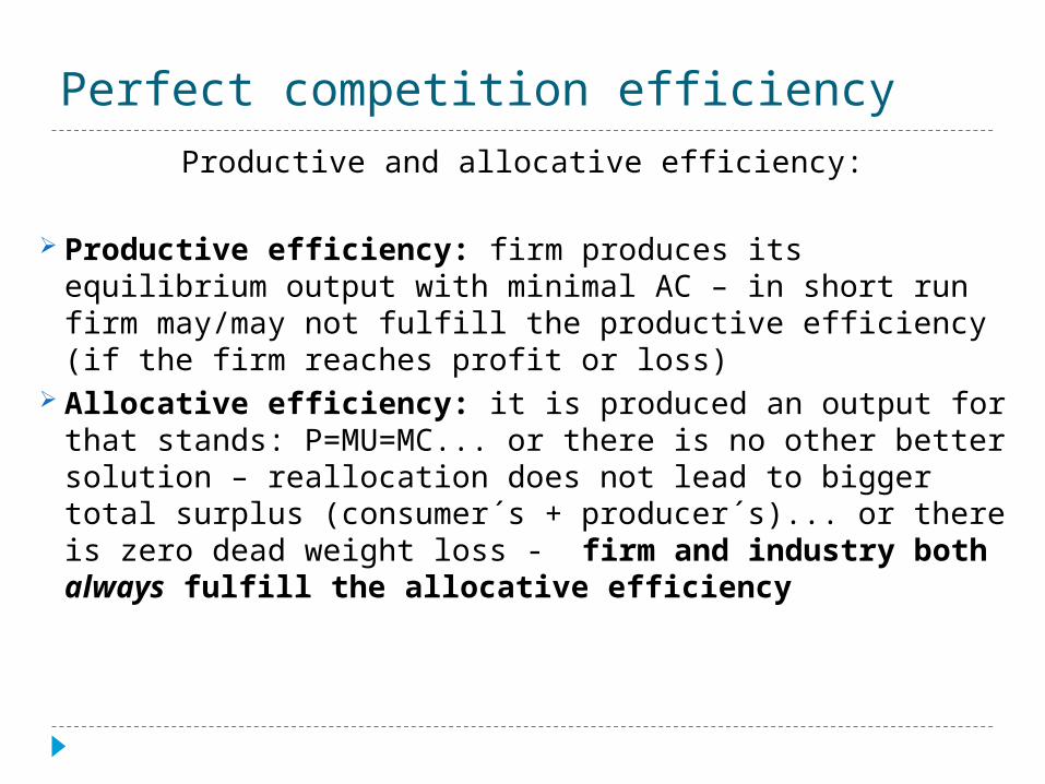
Productive and allocative efficiency:

Productive efficiency: firm produces its equilibrium output with minimal AC – in short run firm may/may not fulfill the productive efficiency (if the firm reaches profit or loss)

Allocative efficiency: it is produced an output for that stands: P=MU=MC... or there is no other better solution – reallocation does not lead to bigger total surplus (consumer´s + producer´s)... or there is zero dead weight loss - firm and industry both always fulfill the allocative efficiency

Allocative efficiency

S

D

Q

P

P*

Q*

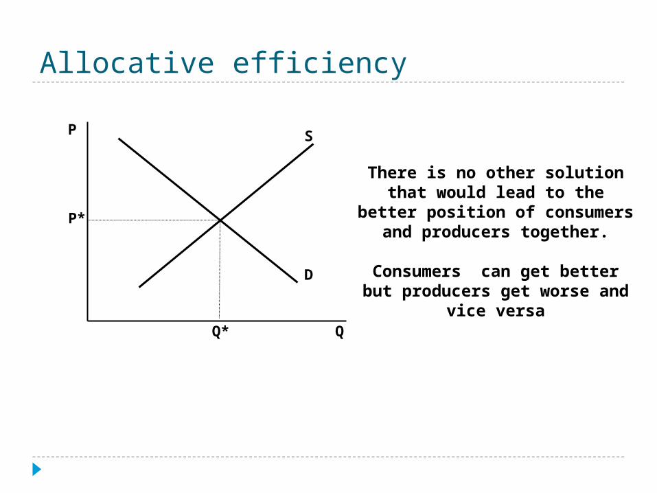
There is no other solution that would lead to the better position of consumers and

producers together.

Consumers can get better but producers get worse and vice versa

Productive efficiency

Q*

CZK/QSMC

SAC

AR=MR=P=d

Q Q*

CZK/QSMC

SAC

AR=MR=P=d

Q

PROFITLOSS

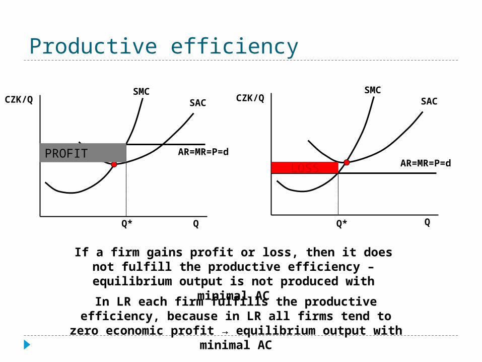
If a firm gains profit or loss, then it does not fulfill the productive efficiency – equilibrium output is not produced with minimal AC

In LR each firm fulfills the productive efficiency, because in LR all firms tend to zero economic profit → equilibrium output with minimal AC

Productive efficiency

Q*

CZK/QLMC

LAC

AR=MR=P=d

Q

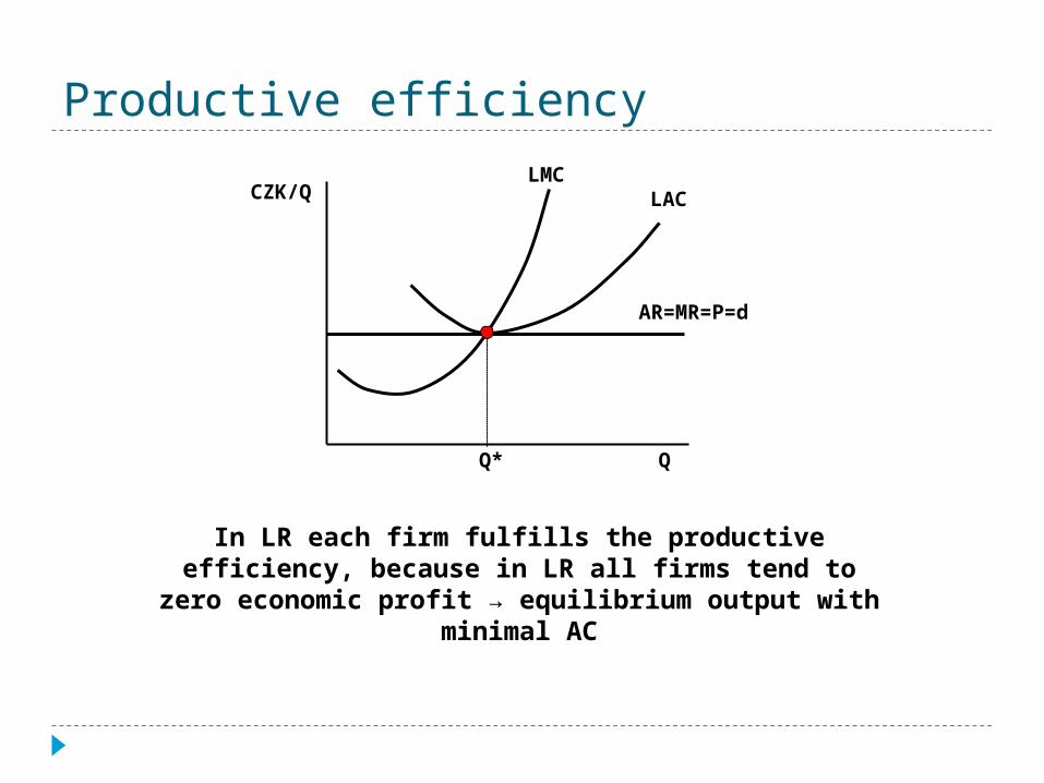
In LR each firm fulfills the productive efficiency, because in LR all firms tend to zero economic profit → equilibrium output with minimal AC

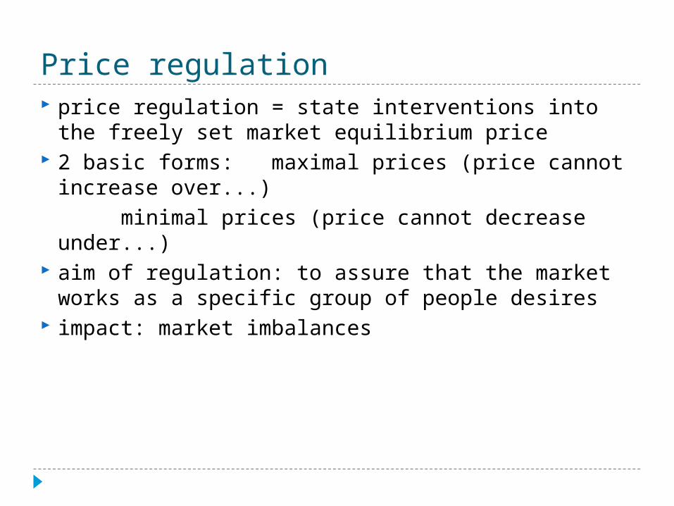
Price regulation price regulation = state interventions into the freely set market

equilibrium price 2 basic forms: maximal prices (price cannot increase over...)

minimal prices (price cannot decrease under...)

aim of regulation: to assure that the market works as a specific group of people desires

impact: market imbalances

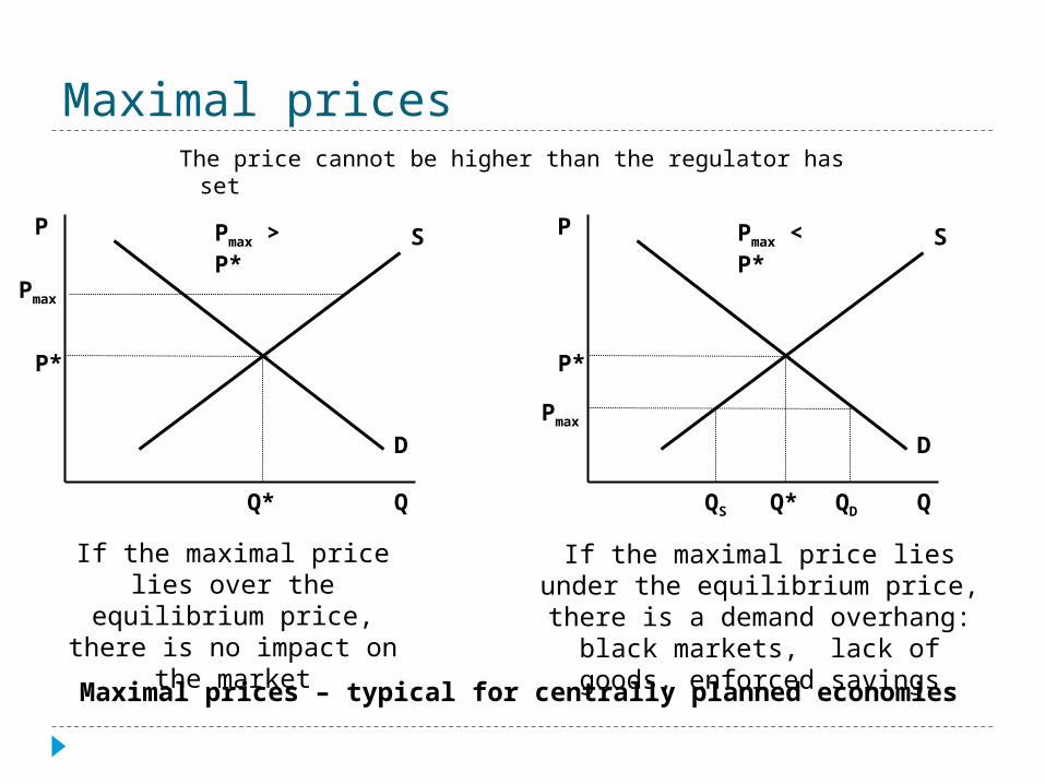
Maximal pricesThe price cannot be higher than the regulator has set

S

D

Q

P

P*

Q*

Pmax

Pmax > P*

If the maximal price lies over the equilibrium price, there is no impact

on the market

S

D

Q

P

P*

Q*

Pmax

Pmax < P*

QS QD

If the maximal price lies under the equilibrium price, there is a demand overhang: black markets, lack of goods, enforced savings

Maximal prices – typical for centrally planned economies

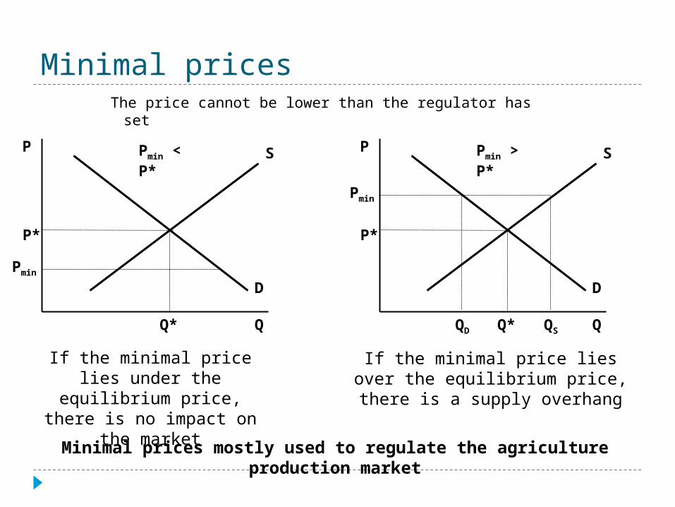
Minimal pricesThe price cannot be lower than the regulator has set

S

D

Q

P

P*

Q*

Pmin

Pmin < P* S

D

Q

P

P*

Q*

Pmin

Pmin > P*

QD QS

Minimal prices mostly used to regulate the agriculture production market

If the minimal price lies under the equilibrium price, there is no impact

on the market

If the minimal price lies over the equilibrium price, there is a supply overhang