Procurement when Price and Quality Matter∗

John Asker†and Estelle Cantillon‡

January 22, 2008

Abstract

A buyer seeks to procure a good characterized by its price and its quality from suppliers who haveprivate information about their cost structure (fixed cost + marginal cost of providing quality).We solve for the optimal buying procedure, i.e. the procedure that maximizes the buyer’sexpected utility. We then use the optimal procedure as a theoretical and numerical benchmark tostudy practical and simple buying procedures such as scoring auctions and negotiation. We findthat scoring auctions are able to extract a good proportion of the surplus from being a strategicbuyer − that is, the difference between the expected revenue from the optimal mechanism andthe efficient auction. Sequential procedures (to which many negotiation processes belong) doless well and, in fact, often do worse than simply holding an efficient auction.

Keywords: optimal auction, multi-attribute auction, differentiated product, multidimensionalscreening, scoring auction, negotiation, bargaining, procurement.

JEL Codes: D44, D82, C78, L24, L22

∗We thank Heski Bar-Isaac, Micael Castanheira, Mathias Dewatripont, Philippe Jehiel, Georg Kirchsteiger, Patrick

Legros, and Nicolas Sahuguet, as well as audiences at the Barcelona workshop on auctions, CEMFI, Paris School

of Economics GREQAM, IDEI Toulouse, LSE, UCL, NYU IO Day, and the Duke-Northwestern-Texas IO Theory

conference for helpful comments, and Alexis Walckiers for his careful proofreading and many expositional suggestions.

Financial support from a FNRS research grant is gratefully acknowledged. This paper supersedes an earlier paper

entitled "Optimal Procurement when both Price and Quality Matter."†Leonard N. Stern School of Business, NYU. Email: jasker@stern.nyu.edu‡FNRS, ECARES (Université Libre de Bruxelles) and CEPR. Email: Estelle.Cantillon@ulb.ac.be

1

1 Introduction

Procurement rarely involves considerations based solely on price. Instead, concerns about the

quality of the good or service provided are often important to the final decision. In this paper,

we consider how a buyer who cares about quality should structure his purchasing process when

suppliers compete for a single procurement contract. We ask two questions: First, what does

the optimal procurement mechanism look like? And, second, how well do simpler, empirically

relevant, mechanisms perform relative to a benchmark constructed using the optimal and efficient

mechanisms?

When suppliers’ private information about their costs can be captured by a one-dimensional para-

meter, the answer to the first question is well known (Laffont and Tirole, 1987, and Che, 1993). In

addition, Che (1993) provides a partial answer to the second question by showing that a scoring

auction implements the optimal mechanism. This paper extends the analysis of the first question

to environments with multidimensional private information and answers the second question more

exhaustively and for several alternative procedures.

Conducting procurement when factors in addition to price matter involves moving toward what

practioners often refer to as ‘complex procurement.’ Large-scale defense aquisitions are an extreme

example of complex procurement − the product involves many dimensions, with varying degreesof contractability, and renegotiation of the contract is expected at many stages. At the other

extreme is the aquisition of basic stationary by a corporation − a pencil is a simple thing and

price is the only factor in the procurement exercise. The mechanisms used in practice to conduct

complex procurement leverage, in varying degrees, the potential competition among suppliers and

the scope for flexibility in product design. When evaluating the performance of simple mechanisms,

we consider two popular examples: a scoring auction and a sequential offer model. The sequential

offer model allows for more flexibity in terms of product design, at the cost of lower competition.

Our results, in answer to the second question posed at the start of this paper, suggest that scoring

auctions do better than sequential procedures and that they often yield a performance close to that

of the optimal mechanism.

The two distinguishing features of our model are that suppliers’ private information about their

cost structure is multidimensional and that quality is contractable and endogenously determined

as part of the procurement process. The U.S. State Highway Authorities’ procurement for highway

repair jobs illustrates these aspects of the contracting environment.1 For high-density traffic areas,

these agencies care about the cost of the job and the time required for completion. A contractor

may be able to speed up the job by hiring extra labor, by using some equipment more intensively,

or by shifting some resources from other jobs. Hence, suppliers’ quality (here, the time they need

to complete the job) is not fixed, but endogenous, with increased quality incurring a higher cost.

Moreover, this marginal cost of quality is likely to vary across potential contractors in a way that is1See, for instance, Arizona Department of Transport (2002) and Herbsman et al. (1995).

2

not observable to their competitors. Therefore, it represents one dimension of private information.

However, there are other sources of unobserved cost heterogeneity. These include the contractors’

material costs, existing contractual obligations and organizational structure, which combine to

determine the fixed cost of undertaking a job at any quality level. Thus, private information is

likely to be better captured by a multidimensional parameter.

We first derive the optimal procurement mechanism in a model where each potential supplier has

private information about two components of her cost structure: her fixed cost and her marginal

cost of providing quality. Costs on each dimension can be high or low, and we allow for any pattern

of correlation between a supplier’s fixed cost and her marginal cost. Across bidders, costs are

independently distributed. The buyer’s objective is to maximize his expected utility subject to the

suppliers’ participation and incentive compatibility constraints.

The optimal procurement mechanism differs significantly from its counterpart in one-dimensional

environments. It depends finely on the exact parameters of the problem, including the number of

suppliers. Moreover, unlike its one-dimensional counterpart, it is not easily amenable to implemen-

tation by a simple-looking auction format. The source of these discrepancies can be traced back

to the well-known endogeneity of the direction in which incentive compatibility constraints bind in

multidimensional screening problems.

The fragility of the intuitions gained from one-dimensional models is endemic in research on multi-

demsional screening, and the largely negative flavor of the results can leave the economist concerned

with the application of mechanism design on unsure footing. In this paper, we take a new approach,

using the characterization of the optimal mechanism to construct a meaningful benchmark to in-

vestigate the performance of practical and simpler buying procedures. In doing so, we suggest one

way in which results from the multidimensional screening literature can be used to constructively

advance our understanding of mechanisms being used in practice.

This benchmark role plays out at two levels. At the theoretical level, we can compare the allocation

(probabilities of getting the contract and qualities delivered) of the optimal mechanism and that of

any other mechanism of interest to understand their advantages and disadvantages.

At a numerical level, the characterization of the optimal mechanism contributes to solving what

is essentially a free-parameter problem in interpreting numerical comparisons. At first glance,

there are at least two candidates for benchmarking numerical simulations of the performance of

simple mechanisms: the optimal mechanism and the efficient mechanism. Unfortunately, neither

of these candidate benchmarks is useful on its own. To illustrate, suppose that, for some set of

parameters, the optimal mechanism generates an expected utility for the buyer of 2, while the

mechanism of interest returns 1. This looks like a 50% decrease in revenue. However, by adding 9

to the buyer’s utility function, we could well generate expected utilities of 11 and 10, respectively.

Now the decrease looks like only 9%. We create a benchmark that is immune to the distortions in

the previous example by looking at the difference between the expected utility generated from the

3

optimal mechanism and the expected utility from the efficient auction. We observe that this is the

surplus available to a strategic buyer and use this measure of ‘stragetic surplus’ as our benchmark

against which to evaluate second-best mechanisms. Suppose that the optimal mechanism returns

an expected utility of 0 (or 9). This allows us to conclude that the mechanism of interest captures

50% of the rents available from being a strategic buyer. This benchmark is both economically

meaningful and free from the influence of (positive) affine transformations of the utility function.

The characterization of the optimal mechanism is crucial to constructing this benchmark.

We apply this new approach to evaluate the performance of scoring auctions and sequential proce-

dures where suppliers are approached one at a time. Our motivation for looking at these procedures

is twofold. First, Asker and Cantillon (2006) have shown that scoring auctions dominate price-only

auctions, beauty contests and menu auctions. Thus, scoring auctions are an obvious candidate for

a simple second-best procedure. Second, buyers often adopt negotiation when quality matters and

our model of sequential procedures bounds many models of negotiation in the existing literature.

We characterize the allocations that can be implemented by a scoring auction (Theorem 2) and

derive the optimal sequential procedure (Theorem 3). By definition, both procedures underperform

against the optimal buying mechanism. The comparison with the allocation generated by the

optimal mechanism highlights several characteristics of these alternatives. First, scoring auctions

can replicate the allocation probabilities of the optimal procedure in many cases. Where scoring

auctions fall short of the optimal auction is in their inflexibility in terms of qualities. Second, the

efficient auction can be implemented by a scoring auction. Thus, scoring auctions can always do

weakly better than the efficient procedure. Third, sequential mechanisms are inherently inefficient

and can never replicate the allocation probabilities of the optimal procedure. However, we identify

two classes of environments where they can do better than the efficient auction thanks to the

distortion in production or in allocation probabilities that they generate.

We further investigate these questions numerically by evaluating the proportion of strategic surplus

that simpler procedures capture, across a wide range of environments. To do this, we compute an

upper bound to the expected utility from these procedures by deriving the optimal scoring auction

and the optimal sequential procedure. We find that the optimal scoring auction does very well and,

on average, captures more than two thirds of the strategic surplus. This result holds for the upper

bound and may not extend for all scoring auctions; therefore we also investigate the performance of

scoring auctions that use “naïve” scoring rules that distort the buyer’s true preferences in the same

direction as the optimal scoring auction, but in an arbitrary way. We find that small deviations from

the buyer’s true preferences often uniformly increase his expected utility. We then turn to sequential

procedures. We find that the optimal sequential procedure does very badly and often even worse

than the efficient auction, except when the fixed and marginal costs are highly correlated, or when

there is little uncertainty about suppliers’ fixed costs. Because these two classes of environments are

near one-dimensional environments, it seems safe to claim that efficient auctions generally dominate

sequential procedures when private information is multidimensional.

4

Related literature. This paper is related to the literatures on procurement and multidimensionalscreening. The literature on procurement is organized around several themes, including the question

of how to take factors other than price into account in the procurement process (Laffont and Tirole,

1987; Che, 1993; Branco, 1997; Ganuza and Pechlivanos, 2000; Rezende, 2003; de Frutos and

Pechlivanos, 2004), the impact of the potential non-contractability of quality (Klein and Leffler,

1981; Taylor, 1993; Manelli and Vincent, 1995; Morand and Thomas, 2002; Che and Gale, 2003),

and the impact of moral hazard and renegotiation (Bajari and Tadelis, 2001; Bajari, McMillan and

Tadelis, 2004). See Che (2006) for an overview.

Our paper fits squarely into the first group and we abstract from the other issues. Our contribution

to this literature is twofold. First, we extend prior analyses of optimal procurement to the richer

environment where private information is multidimensional. Laffont and Tirole (1987) and Che

(1993) characterize the optimal buying mechanism when private information is one-dimensional

(the marginal cost of providing quality). Under some regularity conditions, the optimal buying

scheme distorts the quality provided by the suppliers downwards, relative to their first best levels.

The optimal level of distortion is independent of the number of suppliers, a property known as

the “separation between screening and selection” (Laffont and Tirole, 1987). In addition, except

for the presence of a reserve price, the contract is always allocated efficiently. Finally, Che shows

that a scoring auction with a scoring rule that is linear in price implements the optimal scheme.

Our analysis shows that these results depend heavily on the assumption of one-dimensional signals:

except for the downward distortion of quality, none of these properties holds when we move to a

multidimensional setting. Second, we evaluate existing buying procedures against the benchmark

constructed using the optimal and efficient schemes. Other papers compare the performance of

different procedures: Dasgupta and Spulber (1989), Che (1993) and Chen-Ritzo et al. (2003)

compare the scoring auction, which turns out to be optimal in their setting, with price-only auctions;

Asker and Cantillon (2006) compare the scoring auction with price-only auctions, beauty contests,

and menu auctions; Manelli and Vincent (1995) and Bulow and Klemperer (1996) compare (two

different models of) negotiation with auctions. Except for Asker and Cantillon (2006), all of these

papers are restricted to one-dimensional private information. Moreover, our paper goes beyond

simply ranking procedures, first, by providing a quantitative assessment of the difference in expected

utility and, second, by identifying environments where these alternative procedures are likely to

perform well.

This paper also contributes to the literature in multidimensional screening. Rochet and Stole (2003)

present a recent survey of the contracting applications of multidimensional screening. Auction ap-

plications include the optimal multi-unit auction problems studied by Armstrong (2000), Avery

and Henderschott (2000), Manelli and Vincent (2004) and Malakhov and Vohra (2004), and the

optimal auction with externalities studied by Jehiel et al. (1999). Unlike contracting environments,

our problem involves a resource constraint because the contract can be allocated to only one sup-

plier. Unlike multi-unit auction environments, quality in our problem introduces some non-linearity.

5

Hence, none of the existing characterization results applies to our problem and the method we use

to solve for the solution is somewhat different from the methods used in these papers (even if the

underlying principle is the same).

Through our emphasis on second-best mechanisms, our work echoes the research agenda laid out

in Wilson (1993) of identifying simple and robust second-best mechanisms. Our contribution here

is in leveraging the characterization of the optimal mechanism to analyze second-best candidates

in auction environments with multidimensional private information.

2 Model

We consider a buyer who wants to buy an indivisible good for which there are N potential suppliers.

The good is characterized by its price, p, and its quality, q.

Preferences. The buyer values the good (p, q) at v(q)−p, where vq > 0 (we assume that vq(0) =∞and limq→∞ vq(q) = 0 to ensure an interior solution) and vqq < 0. Supplier i’s profit from selling

good (p, q) is given by p− θi1− θi2q, where θi1 ∈ {l, h} and θi2 ∈ {L,H} (l < h and 0 < L < H.). For

future reference, let ∆θ1 = h− l and ∆θ2 = H −L. Given the binomial support of θ1 and θ2, there

are four supplier types: (h,H), (l,H), (h,L), (l, L), which we denote, for brevity, hH, lH, hL and

lL. We will sometimes use (θ1k, θ2k) to denote supplier type k. For example, (θ1lH , θ2lH) = (l,H).

Note that the buyer and the suppliers are risk neutral.

Social welfare. Let Wk(q) = v(q) − θ1k − θ2kq, the social welfare associated with giving the

contract to type k with quality q. Define WFBk = maxqWk(q). Given the single crossing condition,

qFBlH = qFBhH < qFBhL = qFBlL (to save on notation, we will use the short-hand notation q and q to

describe the first-best levels of qualities, q < q).

Our assumptions, thus far, yield an incomplete ordering of types in terms of the first-best levels

of welfare they generate. To simplify the analysis, we restrict attention to the case where WFBlH <

WFBhL . This assumption does not affect the method we use or the results we get (in particular,

Theorems 2 and 3 do not need this assumption). It simply reduces the number of cases we need

to consider when we characterize the optimal mechanism (Theorem 1). Under this assumption,

having a low marginal cost for delivering a higher-quality product is more important than having a

low fixed cost, at least in the first-best solution. This case includes, as a limit, the case where firms

differ only in their marginal cost parameter, which has been studied by Laffont and Tirole (1987),

Che (1993) and Branco (1997). The natural ordering of types is, thus, lL Â hL Â lH Â hH. Note

that this assumption implies that ∆θ1 −∆θ2q < 0.

Information. Preferences are common knowledge among suppliers and the buyer, with the excep-tion of suppliers’ types, (θ1i, θ2i), i = 1, ...,N, which are privately observed by each supplier. Types

are independently and symmetrically distributed across suppliers, in the sense that the probability

of supplier i being of some type is independent of other suppliers’ types, but the ex-ante distribution

6

of types is the same for all bidders. Thus, we can write the probability of each type as αk > 0,

k ∈ {hH, lH, hL, lL} . Notice that we do not put any restriction on the αk’s, except for the factthat they need to sum to one. Any pattern of correlation between a supplier’s fixed cost and her

marginal cost is allowed.

Note: The 2-by-2 discrete type space considered here is a concession to the practical difficultiesof optimal screening problems in multidimensional environments. Armstrong (1996) and Rochet

and Choné (1998) consider a nonlinear pricing problem in a continuous type-space. Their analyses

suggest that, for tractability, a lot of ex ante structure needs to be imposed at the expense of

economic richness. Our 2-by-2 setting also imposes considerable ex ante structure, but relatively

less of this structure is imposed on the direction of binding IC constraints than would be the case

had a continuous type space been used. Hence, the economic richness of the multidimensional

setting is better preserved. Much of the recent work in multidimensional screening has tended

to focus on discrete type spaces (Armstrong, 2000; Avery and Henderschott, 2000; Malakhov and

Vohra, 2004). In our conclusions, we discuss the applicability of our results to richer informational

environments.

3 Characterization of the Optimal Mechanism

The buyer’s problem is to find a mechanism that maximizes his expected utility from the pro-

curement process. For simplicity, we assume that the buyer buys with probability one (that is,

we assume non-exclusion).2 A direct revelation mechanism in this setting is a mapping from the

announcements of all suppliers, {θ1i, θ2i}Ni=1, into probabilities of getting the contract, the level ofquality to deliver and a money transfer.

Given that the buyer’s preference over quality levels is strictly concave, there is no loss of generality

in restricting attention to quality levels that are only a function of suppliers’ types. Let qk denote

the quality level to be delivered by a type k supplier. This, together with suppliers’ risk neutrality,

implies that suppliers’ payoffs and, thus, behavior depends only on their expected probabilities of

winning and their expected payment. Let xk be the probability of winning the contract conditional

on being type k, and let mk the expected payment she receives. Finally, let Uk denote type k’s

equilibrium expected utility. We have: Uk = mk − xk(θ1k + θ2kqk).

With these simplifications and notation, the buyer’s expected utility from the mechanism is given

2Note that, unlike in environments with continuous multidimensional types (Armstrong, 1996), the assumption of

non-exclusion is not particularly restrictive in discrete type environments. It is easy to find parameter values such

that all virtual welfares in the solution are positive making non-exclusion optimal (this can be seen, for example, in

expression (6) below). Allowing for exclusion would increase the number of cases to consider without adding much in

terms of economics. Its primary effect is to reduce the informational rent that the buyer must give to the non excluded

suppliers. For the rest, the distortions on the x’s and q’s will not be qualitatively different from the non-exclusion

case.

7

by

F (xk, qk, Uk) = NX

k∈{hH,lH,hL,lL}αk(xkWk(qk)− Uk) (1)

The buyer seeks to maximize this expression over contracts (xk, qk, Uk), subject to suppliers’ incen-

tive compatibility (IC) constraints:

Uk ≥ Uj + xj(θ1j − θ1k) + xjqj(θ2j − θ2k) for all k, j ∈ {hH, lH, hL, lL}, (2)

individual rationality (IR) constraints:

Uk ≥ 0 for all k ∈ {hH, lH, hL, lL}, (3)

and subject to the feasibility constraint that the probability of awarding the contract to a subset

of the types is always less than or equal to the probability of such types in the population:

NXk∈K

αkxk ≤ 1− (1−Xk∈K

αk)N for all subsets K of {hH, lH, hL, lL} (4)

Finally, non-exclusion imposes that

NX

αkxkk∈{hH,lH,hL,lL}

= 1 (5)

Border (1991) guarantees that the feasibility constraint is both necessary and sufficient for the

expected probabilities xk to be derived from a real allocation mechanism. This ensures that the

solution to the maximization problem of (1) subject to (2), (3), (4) and (5) is implementable.

The buyer’s problem has four individual rationality constraints, 12 incentive compatibility con-

straints and 15 feasibility constraints. We can simplify them somewhat with the following results:

Lemma 1: Consider the feasibility constraints (4), and define an n-type constraint as a feasibilityconstraint with the relevant subset K having n elements. The following statements hold:

i. At most, one 1-type constraint binds; at most, one 2-type constraint binds; and, at most, one

3-type constraint binds.

ii. These binding constraints are nested, in the sense that the type in the binding 1-type con-

straint must belong to the binding 2-type constraint, and so on.

The proof of Lemma 1 is in the Appendix. The intuition is as follows. Suppose that, at the solution,

the contract is allocated according to the following order of priority: lL Â lH Â hL Â hH, i.e. give

the contract to a type lL if there is one, otherwise to a type lH if there is one, and so on. This

means that the ex-ante probability that a lL type gets the contract is the probability that there

is at least one type lL supplier among the N suppliers − i.e., NαlLxlL = 1 − (1 − αlL)N . Thus

the 1-type constraint binds for lL. It cannot bind for any other types because a binding constraint

for another type would imply that that type has priority over all other types in the allocation, a

contradiction. Next, lL Â lH Â hL Â hH also means that the contract is allocated to a type lL

8

or lH whenever there is one among the N suppliers. This means that the ex-ante probability of a

type lL or lH winning, N(αlLxlL + αlHxlH), is the probability that there is at least one of these

types among the suppliers, 1 − (1 − αlL − αlH)N . Thus, the 2-type constraint binds for {lL, lH},

showing that the binding constraints are indeed nested. Statement (i) of Lemma 1 suggests that it

could be the case that, say, no 1-type constraint binds. This will be the case, for instance, if the

order of priority is lL ∼ lH Â hL Â hH − that is, lL and lH have priority over all the other types

− but if there are a lL type and a lH type, the buyer allocates the contract among them randomly.

In this case, no 1-type constraint binds. Finally, note that the suppliers’ expected probabilities are

weakly aligned with their order of priority in the sense that, if k  j, then xk > xj but if k ∼ j,

then xk T xj .

For future reference, denote the winning probabilities resulting from the efficient allocation (lL ÂhL Â lH Â hH) by xFBk , k ∈ {hH, lH, hL, lL}. Denote the winning probabilities for type lH and

hL resulting from the allocation according to order of priority lL Â lH Â hL Â hH by xmaxlH and

xminhL .

Standard manipulation of the incentive compatibility constraints and the individual rationality

constraints allows us to order the probabilities of winning in a limited way.

Lemma 2: At any solution, xlH ≥ xhH , xlL ≥ xhL and UhH = 0

The key difficulty we face in characterizing the solution to the buyer’s problem is in identifying the

set of binding constraints at the optimum together with the associated partition of the parameter

space. Our approach is to start with the buyer-optimal efficient mechanism. The buyer-optimal

efficient mechanism is the mechanism that implements the efficient allocation in the way most

favorable to the buyer. Efficiency requires that qualities are set such that qlL = qhL = q and

qlH = qhH = q, and that the probabilities are set equal to the first-best probabilities − i.e.,

xk = xFBk for all k. Efficiency does not pin down payments to suppliers when private information

is discrete. The buyer-optimal efficient mechanism (which we will simply refer to as “the efficient

auction”) sets payments to maximize the buyer’s expected utility while satisfying all incentive

compatibility constraints. In practice, only two sets of IC constraints bind at the efficient auction,

as the next lemma establishes:

Lemma 3: When ∆θ1 > ∆θ2q, IClH,hH , IChL,hH and IClL,hL bind in the efficient auction. When

∆θ1 < ∆θ2q IClH,hH , IChL,lH and IClL,hL bind (see Figure 1).

Insert Figure 1 Here

The proof of Lemma 3 can be found in the Appendix. From this starting point, we begin by

progressively adjusting the qualities (the q’s) until the buyer’s utility is maximized conditional on

the x’s or until a new IC constraint binds. If no new IC constraint binds we optimize over the x’s

9

and turn our attention back to the q’s. If a new IC constraint binds, we adjust the x’s and q’s under

the additional constraint imposed by the new binding IC constraint. In this way, we progressively

reach a point where there is no scope for improvement through either changing the x’s or the q’s. At

this point, we will have reached the global maximum as guaranteed by the next lemma. Moreover,

this approach ensures that we cover the entire parameter space since our starting points cover the

whole space. The sketch of proof of Theorem 1 illustrates this approach in more detail.

Lemma 4: The first order conditions of the maximization problem (1) subject to (2), (3), (4) and

(5) are necessary and sufficient for a global maximum.

The proof of Lemma 4 is in the Appendix. It allows us to prove the main result of this section:

Theorem 1: Characterization of the optimal buying mechanismDefine q2hH = argmaxq{WhH(q)− αhL+αlL

αhHq∆θ2} and q2lH = argmaxq{WlH(q)− αhL+αlL

αlHq∆θ2}.

Part I: When ∆θ1−∆θ2q ≥ 0, the probabilities of winning and quality levels in the optimal buyingmechanism are as given in Table 1.

Part II: When ∆θ1−∆θ2q < 0, the probabilities of winning and quality levels in the optimal buyingmechanism are as given in Table 2.

Insert Tables 1&2 Here

Sketch of Proof : The full proof of Theorem 1 is very long (18 pages). Here, we provide only a

proof for solutions 1.1.a and 1.1.b to illustrate our approach to deriving the full characterization.

The reader is referred to the online appendix (provided to referees) for the full proof.

Consider the efficient auction. Let Uk,j be the expected utility of a type k pretending she is of type

j. To ensure incentive compatibility, while minimizing suppliers’ rents, suppliers’ expected utilities

in the efficient auction must be set such that Uk = maxj 6=k Uk,j and UhH = 0..

From Lemma 3, we need to consider only two cases. If ∆θ1 −∆θ2q ≥ 0, the per-supplier buyer’sexpected utility in the efficient auction,

Pk αk[x

FBk Wk(qk)− Uk], is given by:

αlHxFBlH WlH(qlH)− αlHx

FBhH∆θ1 + αhHx

FBhHWhH(qhH) + αhLx

FBhL WhL(qhL)− αhLx

FBhH qhH∆θ2

+αlLxFBlL WlL(qlL)− αlLx

FBhL ∆θ1 − αlLx

FBhH qhH∆θ2

(where all qualities are initially equal to the first-best qualities) or, to highlight the virtual welfare

generated by each supplier:

αlHxFBlH WlH(qlH) + αhHx

FBhH [WhH(qhH)−

αlHαhH

∆θ1 −αhL + αlL

αhHqhH∆θ2] (6)

+αhLxFBhL [WhL(qhL)−

αlLαhL∆θ1] + αlLx

FBlL WlL(qlL)

10

The rents of suppliers lL and hL depend positively on qhH , and the buyer can increase his expected

utility by decreasing qhH , ideally until

q2hH = argmaxqhH{WhH(qhH)−

αlHαhH

∆θ1 −αhL + αlL

αhHqhH∆θ2}

Suppose that no new IC constraint binds in the process. (This will be the case if xFBlH [∆θ1−∆θ2q] >xFBhH [∆θ1 − ∆θ2q2hH ]). Now consider again (6). There is no further scope for improvement by

distorting qualities. Furthermore, the virtual welfare of lL is clearly the largest of all, so that it

is optimal to set xlL = xFBlL . However, the relative ranking of the virtual welfare of lH and hL

is unclear. If WhL(q) − αlLαhL∆θ1 > WlH(q), the virtual welfare generated by supplier hL remains

larger than that of lH, so the optimal allocation is the first-best allocation. This is solution 1.1.a.

Suppose, instead, that the virtual welfare associated with lH is larger than that associated with hL,

itself larger than the virtual welfare associated with hH (formally, and referring to (6), WlH(q) >

WhL(q)− αlLαhL∆θ1 ≥WhH(q

2hH)−

αlHαhH∆θ1− αhL+αlL

αhHq2hH∆θ2). In this case, the buyer would rather

give the contract to supplier lH than to supplier hL − i.e., he would like to change the order ofpriority in the allocation. Increasing xlH while decreasing xhL concurrently (keeping αlHxlH +

αhLxhL +αlLxFBlL constant) does not initially affect any of the virtual welfare, and it increases the

buyer’s expected utility. This process continues until either a new IC constraint binds or we have

reached the feasibility constraint for xlH : N¡αlHx

maxlH + αlLx

FBlL

¢= 1 − (αhL + αhH)

N . Suppose

that we reach xlH = xmaxlH before any new IC constraint binds. The qualities and probabilities are

then all optimized given the binding constraints and lemma 4 guarantees that we have reached the

global maximum. This corresponds to solution 1.1.b. Solution 1.1.c. arises if a new IC constraint

binds in the process. Solutions 1.1.d. and 1.1.e. arise when the ordering of virtual social welfares

is such that type lH is preferred to type hH, which, in turn, is preferred to type hL. End of thesketch of the proof.

Tables 1 and 2 present the main features of the solution. The second column describes the prob-

abilities of winning, and the last four columns describe the qualities at the solution (an interval

means that the optimal level of quality lies in this interval). For instance, Solution 1.2.b has

xlL = xFBlL , which is greater than xhL(< xFBhL ). This is, in turn, greater than xlH¡> xFBlH

¢and

xhH = xFBhH . Both qlL and qhL are at the first best-levels, and qhH ∈ (q2hH , q) and qlH ∈ (q2lH , q).Both are distorted below the first-best level. The conditions that define each solution depend on

the resulting binding constraints and virtual welfares, as summarized in Figures 2 and 3. The value

of the objective function and the value of the control variables at the solution are continuous in the

parameters of the model.

Insert Figure 2 Here

11

The following patterns emerge from the tables. First, because the conditions delimiting the different

cases depend on the probabilities of winning, the solution describing the optimal scheme depends

on the number of suppliers, as well as on the usual parameters of the environment (distributions

of types and cost structure). The dependence of the optimal scheme on the number of bidders is

typical of multidimensional environments where the binding IC constraints are endogenous. No

such effect is present in one-dimensional environments (Laffont and Tirole, 1987).

Second, there is some downward distortion in the quality provided by the high marginal-cost sup-

pliers. The quality provided by the low marginal-cost suppliers is never distorted.

Third, probabilities of winning are also often distorted. Specifically, the probabilities of winning

of the high marginal-cost suppliers are sometimes distorted upwards, whereas the probability of

winning of low marginal-cost supplier hL is sometimes distorted downwards. This is because the

expected surplus of hL can, in turn, affect the information rents of the lL type (while lH’s expected

surplus may not). As a result, reducing xhL (and hence increasing xlH) decreases the information

rents of lL. Note that the allocation of supplier lL is never distorted.

Insert Figure 3 Here

Putting these last two aspects together − productive and allocative distortions − we find no sys-tematic “bias against quality” in the two-dimensional model, unlike in the one-dimensional model

(Laffont and Tirole, 1987 and Che, 1993). While the economic conclusions differ, the underlying

economic motivation is the same: reducing suppliers’ rents. The qualities of the high marginal-cost

types are distorted downwards to reduce the low marginal-cost supplier’s benefit from imitating

them. As illustrated in Figures 3 and 4, all binding constraints between suppliers with different

marginal costs are from the low marginal-cost supplier to the high marginal-cost supplier so this

“trick” is effective. This is also the case in the one-dimensional model where the distortion of high-

cost types’ quality lowers the informational rents of the low cost types. Similarly, the reason why

supplier hL’s probability of winning is sometimes below her first-best level is to reduce supplier

lL’s rent. In each case, the optimal level of distortion balances a trade-off between the costs in

terms of lost social welfare and the benefits in terms of reduced rents.

Lastly, we note that the solution approach differs from that taken in the rest of the literature. The

optimal multi-unit auction problems studied in Armstrong (2000), Avery and Henderschott (2000),

Malakhov and Vohra (2004), and Manelli and Vincent (2004) are linear programming problems.

Candidates for a solution in a linear programming problem are extreme points. The standard

solution technique is to characterize the parameter space over which these extreme points are,

indeed, solutions.Our auction problem is not a linear programming problem but, instead, a concave

programming problem. This is reflected in the solution: both the value of the objective function

and the value of the control variables are continuous in the parameters of the model.

12

Multidimensional screening models that give rise to concave programming problems are studied

by Dana (1993), Armstrong and Rochet (1999), and Armstrong (1999), or Laffont, Maskin and

Rochet (1987) and Rochet and Stole (2002) for continuous-type analogues. The standard solution

technique used in these papers is to posit a set of binding constraints and characterize the parameter

space over which the first-order conditions are satisfied given these binding constraints.

Our problem differs from those considered in these papers in two respects. First, we have many

more constraints: on top of the standard four individual rationality and 12 incentive compatibility

constraints that these problems have in their discrete form, the "auction" aspect of our problem

adds 15 feasibility constraints. Moreover, because it is intrinsically non-separable, our problem lacks

the symmetry of the models in Dana (1993) and Armstrong and Rochet (1999). The consequences

are twofold. First, the number of “solutions” − i.e., configurations of binding constraints at theoptimum − is larger. This is seen in Tables 1 and 2 (Armstrong and Rochet (1999) have, at

most, six solutions to consider). Second, it is harder to reduce a priori the number of constraints

that are likely to bind. By seeking incremental improvements from the efficient mechanism, our

constructive approach to the characterization of the solution guarantees that we cover the entire

parameter space.

4 Scoring Auctions

In practice, implementation of the optimal scheme requires overcoming at least two significant

challenges. First, implementation requires precise knowledge of the environment. Second, in most

instances, implementation of the optimal scheme using a simple, easily explained mechanism is

not possible. This limits the extent to which the market mechanism can be explained to market

participants at low cost and also limits the buyer’s ability to administer procurement at low cost

(since administration would require, for example, highly skilled staff).

These challenges suggest that, for practical purposes, second-best solutions that are simple and

perform well in a variety of settings are likely to be more useful. Commonly used procedures are

obvious candidates. They include scoring auctions, price-only auctions with minimum quality stan-

dards, beauty contests, menu auctions where suppliers can submit several price-quality offers, and

negotiation. Asker and Cantillon (2006) have shown that scoring auctions yield a higher expected

utility to the buyer than a price-only auction with minimum standards and beauty contests, and

that they dominate menu auctions when a second price or an ascending format is used. Hence, our

contenders for second-best procedures are scoring auctions and a sequential offer model that bounds

several negotiation models. We analyze scoring auctions in this section and sequential procedures

in the next.

In a scoring auction, the buyer announces a scoring rule that is linear in price, S(p, q) = ev(q) − p

(with evq ≥ 0, evqq ≤ 0 andmax ev(q)−θ2iq admitting a single interior solution), suppliers submit price-13

quality bids (p, q), and the winner is the supplier whose bid generates the highest score according to

the scoring rule.3 The winner’s resulting obligation depends on the auction format. For example,

in a first-score scoring auction, the winner must deliver a quality level at a price that matches the

score of his bid. In a second-score scoring auction, the winner must deliver a quality level at a price

that matches the second-highest score submitted. Scoring auctions are increasingly used in public

and private procurement and are supported by several procurement software packages (see, Asker

and Cantillon, 2006 for examples and references).

4.1 Theoretical properties

Scoring auctions put some structure on suppliers’ bidding behavior. First, given a scoring ruleev(q)− p, suppliers choose their bids to maximize the score they generate given their profit target,

π, − i.e., they solve max(p,q){ev(q)− p} subject to p− θ1i − θ2iq = π. Substituting for p inside the

maximizer yields

maxq{ev(q)− θ1i − θ2iq − π} (7)

A property of the solution is that it is independent of π, the profit target, and of θ1i, the fixed cost.

Second, a standard incentive compatibility argument establishes that the ordering of suppliers’

winning probabilities must correspond to their ability to generate a higher score (intuitively, define

maxq{ev(q)− θ1i−θ2iq} as the supplier’s type). Thus, a scoring auction will implement a particularallocation if two conditions hold:

1. [production constraint] Given the scoring rule, suppliers maximize (7) by choosing the level

of quality assigned by the allocation.

2. [ranking constraint] The ranking of maxq{ev(q) − θ1i − θ2iq} and, thus, the ranking of thescores are consistent with the assigned probabilities of winning.

The next Theorem characterizes the set of allocations that can be implemented by a scoring auction.

Theorem 2: An allocation can be implemented with a scoring auction if and only if (1) qlH = qhH ,

qhL = qlL with qlH , qhH < qhL, qlL, (2) αlHxlH + αhLxhL = αlHxFBlH + αhLx

FBhL , xhH = xFBhH and

xlL = xFBlL , (3) ∆θ1 − ∆θ2qhL ≤ 0 when xhL > xminhL and (4) ∆θ1 − ∆θ2qlH ≥ 0 whenever the

allocation is such that xlH > xFBlH .

Theorem 2 clarifies the constraints that a scoring auction places on the possible allocations. Its

proof can be found in the Appendix. The first condition says that two suppliers with the same

marginal cost of quality must be providing the same level of quality. Moreover, suppliers with

a lower marginal cost of quality must deliver higher levels of quality at equilibrium. These two

properties follow from the structure of (7). The second condition says that, at equilibrium, type lL

3Asker and Cantillon (2006) refer to this auction format as a quasilinear scoring auction to emphasize the linearity

of the scoring rule in p.

14

must win over any other type, and that type hH must lose against any other type. The reason is

that type lL generates the highest value formaxq{ev(q)−θ1i−θ2iq} for any scoring rule and that typehH generates the lowest such value. The third and fourth conditions follow from the combination

of the production constraint and the ranking constraint. Finally, to prove the sufficiency part of

the claim, we construct a scoring rule that implements the allocation under conditions (1) through

(4).

An immediate consequence of Theorem 2 is that the efficient allocation can be implemented by a

scoring auction. Such a scoring auction has a scoring rule that corresponds to the buyer’s preferences

and uses a second-score format.4 It is both robust, in the sense that it does not depend on the

parameters of the environment, and transparent.

Theorem 2 also clarifies why scoring auctions cannot, in general, implement the optimal solution.

First, qhH and qlH differ generically in the optimal mechanism. Moreover, the optimal mechanism

requires xhH > xFBhH in several cases. This said, scoring auctions have two potential advantages

over the efficient auction. First, they allow for distortion in production. Second, they allow some

distortion in allocation probabilities in the same direction as the optimal procedure. The next

section investigates these properties numerically.

4.2 Computational Results

Having identified the constraints that scoring auctions place on allocations, we next turn to the

question of their relative performance. We interpret the difference between the buyer’s expected

utility from using the optimal mechanism and from using the efficient auction as the surplus avail-

able to a strategic buyer. We ask to what extent scoring auctions capture this surplus. We answer

this question in two steps. First, we compute a tight upper bound to the performance of scoring

auctions by computing the expected utility generated by the optimal scoring auction. Second, we

analyze the performance of naïve scoring auctions − that is, scoring auctions that use scoring rulesthat differ from the optimal scoring rule in an arbitrary way.

4.2.1 Bounds

To evaluate the performance of scoring auctions, we compute an upper bound to the expected utility

that scoring auctions generate by adding the constraints of Theorem 2 onto the initial problem and

solving the resulting program numerically. The resulting expected utility is then compared with the

expected utility from the efficient auction and the expected utility from the optimal mechanism.

4To ensure that the scoring auction generates as much utility to the buyer as possible, type-specific down-payments

must be included. These down-payments are an artifact of the discrete type space where allocations do not fully pin

down payments. They maintain incentive compatibility and increase the buyer’s utility. See Fudenberg and Tirole

(1991) for more details.

15

Insert Figure 4 Here

Figure 4 shows the results for an environment where v(q) = 3√q, l = L = 1, H = 2, N = 2

and αk = 0.25. The value of ∆θ1 varies along the x-axis. The expected utility from the optimal

mechanism lies above that from the optimal scoring auction, which, in turn, dominates that from

the efficient auction. As the value of ∆θ1 increases, the expected utility decreases in all three

mechanisms. This is to be expected. When ∆θ1 increases, the maximum level of welfare decreases

because suppliers’ costs increase. Moreover, fixed costs become relatively more important as a

source of adverse selection. The kink at the point ∆θ1 = 0.5625 corresponds to the point when

the binding incentive compatibility constraint for type hL in the efficient mechanism switches from

IChL,lH to IChL,hH (thus ∆θ1 = ∆θ2q). The resulting increases in the weight of ∆θ1 in the buyer’s

expected utility explains the kink.5

We replicated this exercise for a range of environments by varying the values for the αk’s and some

of the other parameters of the model. Table 3 reports the results. The third column reports the

average proportion of the strategic surplus captured over the full range of values that ∆θ1 can

take. The fourth column reports the maximum percentage of the surplus that the optimal scoring

auction captures together with the corresponding value of ∆θ1. The fifth column does the same for

the worst relative performance of the optimal scoring auction. Finally, columns 6 and 7 report the

percentage of ∆θ1 values for which the performance of the optimal scoring auction is greater than

80% (column 6) or within ten percentage points of its worst performance (column 7). For the core

set of experiments (experiments 1 through 20), v(q) = aqb with a = 3 and b = 0.5, l = L = 1, h = 2,

N = 2. The bottom part of the table considers other values for a, b, L and H. (We keep N = 2 in

all our experiments because this is where the actual choice of mechanisms is likely to matter most).

Figure 5 shows the relative performance of the optimal scoring auction as ∆θ1 changes for selected

probability configurations.

Insert Table 3 Here, Insert Figure 5 Here

The results are as follows. First, in every experiment, there exists a value of ∆θ1 for which

the optimal scoring auction does as well as the optimal mechanism. Second, the point at which

this occurs seems somewhat persistent across environments. Third, the optimal scoring auction

5As ∆θ1 tends to 0, the source of adverse selection reduces to one dimension, the marginal cost. In this case, Che

(1993) has shown that a scoring auction implements the optimal mechanism. The reason why the expected utility

from the optimal scoring auction does not converge to the expected utility of the optimal mechanism in our graph

is that there is some discontinuity in the optimal scoring auction at ∆θ1 = 0. As long as ∆θ1 > 0, scoring auctions

impose that lH generates a strictly higher score than hH. Thus xlH ≥ xFBlH > xhH = xFBhH (Theorem 2). This leaves

some informational rent to lH and increases the rents of hL and lL relative to the case where xlH = xhH . When

∆θ1 = 0, suppliers lH and hH are essentially the same. The optimal scoring auction will, thus, set xlH = xhH and

leave no rent to supplier lH.

16

captures, on average, more than two thirds of the strategic surplus, even though this proportion

can dip down to 20% for some values of ∆θ1 and some environments. Fourth, the optimal scoring

auction does worst when the fixed cost and the marginal cost are negatively correlated. We now

investigate each of these points in more detail.

In every experiment, there exists a value of∆θ1 for which the optimal scoring auction does as well as

the optimal mechanism. Given Theorem 2, this must happen at parameter values such that there

are binding incentive compatibility constraints directed to both lH and hH from low marginal-

cost suppliers in the optimal scheme (otherwise, there is no chance that the qualities provided by

suppliers lH and hH are the same in the optimal scheme). Inspection of Tables 1 and 2 suggests

that the only candidates consistent with implementation with a scoring auction are solutions 1.1.c.,

1.2.a, 1.2.b or 1.2.c. (Recall that scoring auctions require xhH = xFBhH ). Closer inspection of the

numerical solution suggests that the maximum performance of the optimal scoring auction happens

when the optimal mechanism corresponds to either solutions 1.2.a, or 1.2.c.

An inspection of Figure 5 and the results in Table 3 suggests that the optimum is reached at a

similar region in each set of simulations (in particular, this point is always less than 0.5625, the

point at which the binding incentive compatibility constraint for type hL in the efficient mechanism

switches from IChL,lH to IChL,hH). This raises the question of why there and not elsewhere? The

parameter setting in figure 5 where the probabilities are (35, 35, 15, 15) suggests that it is possible

for the optimum revenue to be generated to the right of the dip in revenue. To investigate this,

we ran a set of experiments for the probabilities (40, 40, 10, 10) and (45, 45, 5, 5): experiments 17

and 18 . In this setting, the solution corresponds to solution 1.1.d in table 1. In experiment 17,

at ∆θ1 = 0.93375, the optimal scoring auction captures 99.03% of the available strategic surplus,

whereas, at ∆θ1 = 1.02375, this is raised to 99.89%. While it appears that the scoring auction

does well in these regions, it falls short of the optimal mechanism because of the restriction that

xhH = xFBhH in the scoring auction.

It has been noted that the point at which the optimal scoring auction does as well as the optimal

scheme is constant across cases 1-5 and 10-15. After further inspection, this is an artifact of the

common symmetric structure of these parameter settings. These settings are such that αlL = αhH

and αhL = αlH . A comparison with experiments 6 and 19 illustrates this point: In experiment 6,

the probabilities are such that αlL = αhL > αlH = αhH , resulting in a move in the location of the

optimum; experiment 19 makes a similar perturbation, with the additional shock that αlH < αhH .

The optimal scoring auction does very well overall. It captures, on average, more than two thirds

of the surplus, and in ten of the 13 core experiments reported in Table 3, it captures more than

80% of the surplus for the majority of the values ∆θ1 can take. This excellent performance seems

attributable to the relative flexibility that scoring auctions leave in terms of allocation.

Table 3 and Figure 5 also indicate that scoring auctions perform less well in some environments.

This poor performance tends to happen around the point at which there is a kink in the expected

17

utility of the efficient auction. This coincides with the point at which both incentive compatibility

constraints out of type hL are close to being binding in the efficient mechanism (one must bind,

and the other is ‘close’ to binding). As a result, those IC constraints leave little scope for rent

extraction before they bind. Given that the scoring auction is less flexible in the face of these

constraints than the optimal mechamism, it is not surprising that its relative performance suffers.

Similarly, a negative correlation between the marginal cost and the fixed costs decreases the per-

formance of the optimal scoring auction (see experiments 4, 5 and 15). Intuitively, a negative

correlation moves the environment further from the one-dimensional environment for which scoring

auctions are known to do well (Che, 1993). The weight of types lH and hL is large in the total

expected utility of the buyer, and so the gains from distorting quality tend to make qhH far from

being first-best. In light of this, it is noteworthy that a positive correlation does not unambiguously

generate strong performances from the scoring auction. In experiments 2 and 3, where the extent

of the positive correlation is increasing, the scoring auction appears to be doing increasingly well.

However, in experiment 14, this trend does not continue. What is happening here is that the extra

flexibility in the optimal mechanism is able to exploit the environment as it moves toward the

one-dimensional case far sooner than the scoring auction. The relative performance of the scoring

auction in experiment 14 reflects a reconfiguration of the optimal mechanism in the face of the

changing environment, rather than any significant change in the scoring auction itself.

4.2.2 Simple manipulations of the scoring rule

While consideration of the optimal scoring auction is fruitful, it remains an upper bound. Moreover,

the optimal scoring auction also depends finely on the parameters of the environment. For this

reason, we investigate the performance of “naïve scoring auctions.” Naïve scoring auctions are

scoring auctions that use scoring rules that differ from the true preferences of the buyer in an

arbitrary way (but in the same direction as recommended by the optimal scheme), independently

of the parameters of the environment.

Let v (q) = aqb. We consider the expected utility generated by a scoring auction with scoring rule

a∗qb−p and a∗ = (0.9)a or a∗ = (0.95)a. Thus, the winner is the supplier who generates the highestvalue for maxq{a∗qb − θ1i − θ2iq}, and she receives the value of the second-highest score.6

Insert Figure 6 Here, Insert Table 4 Here

Figure 6 shows the proportion of the strategic surplus captured by the naïve scoring auction when

a∗ = (0.95)a and αk = 0.25. At first, the proportion of surplus is at 14% and then increases up to

38%. At this point, the binding IC constraints change in the naïve scoring auction: IChL,hH ceases

to bind and IChL,lh starts binding. This causes a sharp drop in the proportion of surplus extracted

6As before, some adjustments need to be made to account for the discreteness of the types space.

18

by the naïve scoring auction. The next major shift is the dramatic increase in the proportion

of surplus captured when ∆θ1 ' 1. This happens when the naïve scoring auction distorts the

probabilities of winning by giving priority to type lH over type hL. Because the virtual welfare

(as measured using the buyer’s true utility function) generated by type lH is also higher than the

virtual welfare generated by type hL at this point, this increases expected utility sharply.

Table 4 summarizes the results of this exercise repeated for the parameters of the core experiments.

The qualitative results in Figure 6 are replicated in all experiments. Table 4 reports the range of

performance for the naïve scoring auction when it allocates the contract in the same way as the

efficient auction does (column 4) and when it allocates the contract differently by giving priority to

type lH over type hL. The results show that the naïve scoring auction does particularly well when

it distorts the allocation probabilities. This suggests that, for rent extraction purposes, distortions

in the allocation probabilities are more important than distortions in qualities.

5 Sequential procedures

We now turn to sequential procedures. Sequential procedures are mechanisms that approach sup-

pliers at most once. Several practical procedures belong to this category, including many models

of negotiation. These include a procedure in which the buyer negotiates with a single supplier and

walks out if the supplier does not offer him a certain level of utility; a procedure whereby the buyer

makes sequential take-it-or-leave-it price offers (as in Manelli and Vincent, 1995); and a procedure

where the buyer pre-selects a single supplier and offers him a menu of optimal screening contracts

(as in Wang, 1998).

5.1 Theoretical properties

Our purpose here is to get a sense of the costs and benefits of sequential procedures relative to

the efficient auction, the optimal procedure, and procedures that allow the suppliers to complete

directly with each other (i.e., this case represented by the scoring auction). As before, we use the

strategic surplus available to the buyer to benchmark the performance of sequential procedures. To

do this, we characterize the optimal sequential procedure − i.e., the mechanism that maximizes thebuyer’s expected utility conditional on approaching suppliers at most once. This optimal sequential

procedure provides an upper bound to what sequential procedures can achieve because it gives all

bargaining power to the buyer.

The optimal sequential procedure solves a simple dynamic programming problem. The buyer

approaches suppliers one at a time and offers them a menu of optimal screening contracts that

takes into account the number of remaining suppliers.7 Because suppliers are approached only

7 In that sense, the optimal sequential procedure combines the features of Wang (1998)’s single-buyer single-supplier

optimal negotiation and those of Manelli and Vincent (1995)’s sequential model of negotiation.

19

once, their dominant strategy is to accept the best offer that meets their individual rationality

constraint. If a supplier refuses, the buyer turns to the next supplier. To ensure that we can compare

our results with the results of the previous sections, we require that the contract is allocated with

probability one, which implies that the offers made in the last round must be acceptable to all

types of suppliers.8 The next Lemma shows that, in any round, we can, without loss of generality,

consider a menu of two contracts, one targeted at the low marginal-cost suppliers, and the other

targeted at the high marginal-cost suppliers. The intuition is that contracts of the form (p, q) are

unable to screen over suppliers’ fixed cost, θ1.

Lemma 5: In any round, the buyer offers at most two contracts.

Proof: Towards a contradiction, suppose that the buyer offers three contracts and, without loss ofgenerality, suppose that one, (plL, qlL), is targeted at lL and another, (phL, qhL) is targeted at hL.

Incentive compatibility requires:

plL − θ1 − θ2qlL ≥ phL − θ1 − θ2qhL

phL − θ1 − θ2qhL ≥ plL − θ1 − θ2qlL

Thus, plL − θ2qlL = phL − θ2qhL, and the contracts lie on an isoprofit locus for suppliers hL and

lL, {(p, q) : plL − θ2qlL = phL − θ2qhL}. Since the buyer has strictly convex preferences, there is aunique contract on this locus that maximizes his utility. Q.E.D.

Let (pn1 , qn1 ) and (p

n2 , q

n2 ) denote the menu of contracts offered when n suppliers remain, with the

convention that qn1 ≤ qn2 . In the last round, the buyer’s optimization problem is given by

max(p1,q1),(p2,q2)(αlH + αhH)(v(q1)− p1) + (αhL + αlL)(v(q2)− p2)

subject to suppliers’ IR and IC constraints. Following standard arguments, supplier hH’s IR

constraint is binding − i.e., p1 = θ1 + θ2q1 − and only the downward IC constraint is binding −i.e., p2 − θ2q2 = p1 − θ2q1. Substituting for p1 and p2 in the objective function yields:

max(p1,q1),(p2,q2)(αlH + αhH)(v(q1)− θ1 − θ2q1) + (αhL + αlL)(v(q2)− θ1 − θ2q2 −∆θ2q1)

This establishes Lemma 6:

Lemma 6: The optimal take-it-or-leave-it offer in the last round is given by (p11, q11), where

p11 = θ1 − θ2q11 and q11 = argmax{v(q)− θ2q − (αhL+αlL)

(αlH+αhH)q∆θ2}, and (p12, q12) = (p11 + θ2(q − q11), q).

The resulting continuation value is given by (αlH+αhH)WhH(q11)+(αhL+αlL)(W

FhHhL (q)−∆θ2q11).

Let Vn denote the continuation value of a buyer facing n remaining bidders. We are now ready to

characterize the optimal sequential procedure:

8As for the optimal procedure, such a requirement can be perfectly consistent with optimality if the buyer values

the good sufficiently highly. In that case, exclusion in the last period is suboptimal.

20

Theorem 3 (characterization of the optimal sequential procedure): The optimal sequentialprocedure is such that the buyer offers the menu of contracts defined in Lemma 6 in the last round

and, when n > 1, one of the four pairs of contracts in Table 5, depending on which one yields the

largest continuation value (conditional on the condition in the third column being satisfied):

Insert Table 5 here

(Suppliers of types lH and hH accept the contract (pn1 , qn1 ) if it satisfies their IR constraint, and,

likewise, suppliers of types lL and hL accept contract (pn2 , qn2 ) if it satisfies their IR constraint).

Proof: See Appendix

Note that q∗∗1 < q∗1, so that Kn = {lL, lH} and Kn = {lL, lH, hL} cannot happen for the sameparameter values.

The optimal sequential procedure has two potential advantages. First, it can distort production.

Second, it can distort the probabilities of winning. For example, a first-period offer that is accept-

able only to suppliers lL and lH distorts the probabilities that lH wins, xlH , upwards and distorts

xhL downwards relative to the probabilities in the efficient auction, as is sometimes required in the

optimal procedure. However, this comes at the cost of a distortion in the probabilities of allocating

the contract to types lL and hH. Indeed, it is easy to check that xlL < xFBlL , unless the optimal offer

in all rounds but the last is acceptable only to type lL (and recall from Theorem 1 that xlL = xFBlLalways in the optimal procedure). In addition, xhH > xFBhH in all cases except if Kn = {lL, lH, hL}for all n > 1.

These costs and benefits of the optimal sequential procedure are best illustrated for the case of two

suppliers. To do this, we rewrite the expected utility from the efficient auction asP

pkVWk, where

pk is the probability that the mechanism allocates the contract to a type k supplier and VWk is the

associated virtual welfare. Table 6 summarizes the values that these variables take in the efficient

auction (using Lemma 3):

Insert Table 6 Here

Similarly, the expected utility from the optimal sequential procedure can be written asPepkgVW k

where epk is the probability that the optimal sequential mechanism allocates the contract to supplierk and gVW k is the "resulting" virtual welfare.9 The idea, then, is to compare the pk’s with theepk’s and the VWk’s with the gVW k’s. The first example illustrates the advantage of being able to

distort qualities.

9We write “resulting” because the virtual welfare associated with a given type is not uniquely pinned down in this

sequential mechanism. We exploit this flexibility in the remaining discussion.

21

Example 1: The optimal sequential procedure always captures a positive proportionof the strategic surplus when ∆θ1 is sufficiently small. We prove this by showing thatP

pkVWk <PepkgVW k. When ∆θ1 is small, the main source of adverse selection is marginal cost,

and suppliers lL and hL, and lH and hH, respectively, are very much alike. Consider the strategy

that consists of making an offer that is acceptable only to suppliers lL and hL in the first period.

Using Lemma 6 and Theorem 3, the resulting expected utility is given by:

V2 = (αhL + αlL)WFBhL + (αlH + αhH)V1

= αlL(2− αhL − αlL)WFBlL

+αhL(2− αhL − αlL)

µWFB

hL −αlLαhL∆θ1

¶+(αlH + αhH)

2

µWhH(q

11)−

(αhL + αlL)

(αlH + αhH)∆θ2q

11

¶where we have grouped types lH and hH. Comparing this expression with the second column of

Table 5 suggests that VWlL = gVW lL and VWhL = gVWhL. Moreover, phL + plL = 1− (1− αhL −αlL)

2 = ephL+eplL = (αhL+αlL)(2−αhL−αlL). Thus, when∆θ1 is very small, plLVWlL+phLVWhL 'eplLgVW lL + ephLgVWhL since VWhL ' VWlL. Turning to the utility contribution of types lH and

hH in the efficient auction, we get, using Table 5 and after some simplifications:

αlH(αlH + 2αhH)WFBlH + α2hHW

FBhH − (αlH + 2αhH)(αhL + αlL)∆θ2q

+((αlH + αhH)(αhL + αlL)− αlHαhH)∆θ1

= (αlH + αhH)2

∙WFB

hH −(αlH + 2αhH)(αhL + αlL)

(αlH + αhH)2∆θ2q

¸+(αlH + αhH)(1− αhH)∆θ1

The first term of this expression is strictly less than (αlH + αhH)2³WhH(q

11)− αhL+αlL

αlH+αhH∆θ2q

11

´given the way q11 is constructed (optimal level of distortion) and the fact that

(αlH+2αhH)(αhL+αlL)(αlH+αhH)2

>αhL+αlLαlH+αhH

. The second term becomes negligible as ∆θ1 decreases. Thus, when ∆θ1 is small enough,

the optimal sequential procedure dominates the efficient auction because it is able to distort qual-

ities. End of example 1.

Another way to view example 1 is to note that as ∆θ1 converges to zero, the environment converges

essentially to the "standard" one-dimensional environment, where the optimal procedure is such

that lL and hL win over hH and lH and qualities are distorted. The sequential procedure replicates

these features when K2 = {lL, hL}. In fact, the expected utility from the optimal sequential

procedures converges to the expected utility from the optimal mechanism as ∆θ1 decreases (see

Table 6 below for numerical evidence on this).

The next example illustrates the advantage provided by the ability to distort allocation probabilities:

Example 2: For large values of ∆θ1, the optimal sequential procedure can capture apositive fraction of the strategic surplus. Again, we prove this by showing that

PpkVWk <

22

PepkgVW k. Consider the period 1 strategy that offers a contract to types lL and lH only. The

resulting expected utility for the buyer is given by:

V2 = αlL(WFBlL −∆θ2q∗1) + αlHWlH(q

∗1) + (1− αlH − αlL)V1

= αlL(2− αlH − αlL)WFBlL

+αhL(1− αlH − αlL)(WFBhL −

αlLαhL∆θ1)

+αlH(2− αlH − αlL)

µ1

(2− αlH − αlL)WlH(q

∗1) +

(1− αlH − αlL)

(2− αlH − αlL)WlH(q

11)

¶+αhH(1− αlH − αlL)

µWhH(q

11)−

αlHαhH

∆θ1 −(αhL + αlL)

αhH∆θ2q

11 −

αlLαhH(αhH + αhL)

∆θ2q∗1

¶=

Xk

epkgVW k

Comparing this with the probabilities and the levels of virtual welfare in Table 5, it is clear that

VWlL = gVW lL, V WhL = gVWhL, V WlH > gVW lH and VWhH ≶ gVWhH . Moreover, the sequential

procedure essentially places lH in front of hL in the order of priority in the allocation, resulting in

the following ordering of probabilities: plL > eplL, phL >> ephL, plH << eplH and phH < ephH . WhenαlLαhL∆θ1 is large enough, VWhL << VWlH , gVW lH . Thus, this allocation can increase expected

utility. End of example 2

Figure 7 illustrates an environment in which both of these scenarios occur. Figure 7 compares the

performance of the optimal sequential procedure and that of the efficient auction. For low and high

values of ∆θ1, the optimal sequential procedure does better than the efficient auction, implying

that it captures a positive fraction of the strategic surplus for these parameters. It does worst

elsewhere.

Insert Figure 7 Here

5.2 Computational results

The previous analysis has identified conditions in the environment that favor sequential mechanisms.

Another question concerns the relative performance of sequential mechanisms across a wide range of

environments. Table 7 reports the proportion of the strategic surplus that the optimal sequential

procedure captures. In the table, v(q) takes the form aqb, where a = 3 and b = 0.5. In all

experiments, l = L = 1, H = 2 and N = 2. Negative values indicate that the optimal sequential

mechanism does worse than the efficient auction.

Insert Table 7 Here

The results as follows. On average (i.e., across all possible values of ∆θ1), the optimal sequential

procedure does worse, and often much worse, than the efficient auction. Hence, it necessarily does

23

worse than the optimal mechanism and a scoring auction. The poor performance of sequential

mechanisms is confirmed by the small fraction of values for ∆θ1 where the optimal sequential

mechanism captures at least 80% of the surplus (second-to-last column) and where it does better

than the efficient auction (last column).

There are two exceptions to the poor performance of sequential procedures. First, and as suggested

by example 1, the optimal sequential procedure does very well and, in fact, as well as the optimal

mechanism when ∆θ1 = 0 (fourth column in the table).

Second, the optimal sequential mechanism does better overall when there is strong positive corre-

lation between types (experiment 4 in the table). The reason is related to example 2 above: when

costs are highly correlated, αlLαhL

is high, and the virtual welfare associated with type hL tends to

be lower than the virtual welfare associated with lH. Thus, a contract acceptable only to types

lH and lL in the first period reverses the order of priority of types hL and lH and can increase

expected utility. Note, however, that this is not the end of the story. Indeed, the optimal sequential

procedure does poorly in experiments 17 through 19, even though the ratio αlLαhL

is high there too.

The reason is that a first-period offer acceptable to types lL and lH also increases the probability

that a type lH wins over a type lL. Experiments 17 through 19 illustrate that this is particularly

costly in terms of expected utility when αlH > αlL.

It is clear that, as compared to the performance of scoring auctions, sequential procedures appear

largely unattractive in these simulation environments.

6 Concluding remarks

In this paper, we have asked how a buyer should optimally structure his buying process when sup-

pliers’ private information is multidimensional and quality is contractable, and how well commonly

used procedures such as scoring auctions and sequential procedures perform. We have answered the

second question by combining a theoretical analysis of the restrictions that such simpler procedures

impose on allocations with numerical analyses of their performance relative to the strategic surplus

generated from using the optimal buying mechanism.

Our main results are that scoring auctions do well and that sequential procedures do poorly. In

each case, we have identified the underlying reason and environments that represent exceptions to

this general result. Our interpretation of both sets of results is that utility maximization is more

about “getting allocation probabilities right” than about distorting qualities. This is the main

reason why scoring auctions do well and sequential procedures do so poorly. Because the scoring

auction’s “right kind of flexibility in terms of allocation probabilities” and the generic misallocation

of contracts in sequential procedures are intrinsic features of these procedures and do not depend

on the number of bidders, we are confident that the bottom line of our numerical results extends to

more than two suppliers (Of course, as the number of suppliers goes to infinity, it is straightforward

24

to show that the expected utility from all procedures converge to the same value, which is WFBD -

full extraction). From a practical perspective, our advice to professional buyers is: use a scoring

auction and manipulate it slightly if you can commit, otherwise just announce your true preferences

regarding the price-quality tradeoff.

An a priori restrictive assumption in our analysis is the binary structure of private information,

and it is worthwhile to comment on it here. First, we note that the main results concerning the

optimal procedure (such as the facts that it depends on the number of bidders, that it involves both

productive and allocative inefficiencies, and that suppliers with the same marginal cost for quality

generically supply different quality levels) are all driven by the endogeneity of the binding incentive

compatibility constraints. For this reason, we expect them to hold in more general environments.

Second, the generic misallocation of the sequential procedure can only become worse in richer

informational environments, whereas scoring auctions continue to allocate the contract efficiently,

conditional on the announced scoring rule. Thus, under the (reasonable) conjecture that optimal

allocation is the first-order issue in these complex procurement settings, then the dominance of

scoring auctions is likely to extend to these richer environments.

The poor performance of sequential procedures in our paper is in stark contrast with the popularity

of negotiation for complex procurement among practitioners. This might be due to procurement

managers’ intrinsic preference for procedures over which they have control or to objective factors not

modelled in this paper, such as unknown preferences, non-contractability, renegotiation, or other

moral hazard-type issues. Those objective factors may provide a rationale for using negotiation over

scoring auctions in complex procurement. Studying their impact on the performance of negotiation

is a venue for further research.

25

References

[1] Arizona Department of Transport (2002), A+B Bidding Guide,

http://www.dot.state.az.us/roads/constgrp/A+BGuide.pdf (dated 1/18/2002).

[2] Armstrong, Mark (1996), Multiproduct Non-linear Pricing, Econometrica, 64, 51-74.

[3] Armstrong, Mark (2000), Optimal Multi-Object Auctions, Review of Economic Studies, 67,

455-481.

[4] Asker, John and Estelle Cantillon (2006), Properties of Scoring Auctions, NYU and ECARES

mimeo

[5] Avery, Chris and T. Henderschott (2000), Bundling and Optimal Auctions of Multiple Objects,

Review of Economic Studies, 67(3), 483-497.

[6] Bajari, Patrick, Robert McMillan and Steve Tadelis (2004), Auctions vs. Negotiation in Pro-

curement: An Empirical Analysis, mimeo.

[7] Bajari, Patrick and Steve Tadelis (2001), Incentives Versus Transaction Costs: A Theory of

Procurement Contracts, Rand Journal of Economics, 32(3), 287-307

[8] Border, Kim (1991), Implementation of Reduced Form Auctions: A Geometric Approach,

Econometrica, 59(4), 1175-1187.

[9] Branco, Fernando (1997), The Design of Multidimensional Auctions, Rand Journal of Eco-

nomics, 28(1), Spring 1997, pp. 63-81

[10] Bulow, Jeremy and Paul Klemperer (1996), Auctions versus Negotiation, American Economic

Review, 86(1), 180-194.

[11] Che, Yeon-Koo (1993), Design Competition through Multidimensional Auctions, Rand Journal

of Economics, 668-680.

[12] Che, Yeon-Koo and Ian Gale (2003), Optimal Design of Research Contests, American Eco-

nomic Review, 93,

[13] Che, Yeon-Koo (2006), Procurement, forthcoming The New Palgrave. Dictionary of Economics

(S. Durlauf and L. Blume, Eds), Second Edition.

[14] Chen-Ritzo, Harrison, Kwasnica and Thomas (2003), Better, Faster, Cheaper: a multi-

attribute supply chain auction mechanism, Penn State mimeo.

[15] Dasgupta, S. and D. Spulber (1989), Managing Procurement Auctions, Information Economics

and Policy, 4, 5-29.

26

[16] De Frutos, Maria-Angeles and Lambros Pechlivanos (2004), Auctioning Off with a Split Mind:

Privatization under Political Constraints, Carlos III mimeo.

[17] Ganuza, Juan-Jose and Lambros Pechlivanos (2000), Heterogeneity Promoting Procurement,

Economics Letters, 67(1), 105-112.

[18] Herbsman, Zohar, Wei Tong Chen and William C. Epstein (1995), Time is Money: Innova-

tive Contracting Methods in Highway Construction, Journal of Construction Engineering and

Management, 121(3), 273-281.

[19] Jehiel, Philippe, Benny Moldovanu and Ennio Stachetti (1999), Multi-dimensional Mechanism

Design for Auctions with Externalities, Journal of Economic Theory, 85(2), 258-94.

[20] Klein, B. and K.B. Leffler (1981), The Role of Market Forces in Assuring Contractual Perfor-

mance, Journal of Political Economy, 89, 615-41.

[21] Laffont, Jean-Jacques and Jean Tirole (1987), Auctioning Incentive Contracts, Journal of

Political Economy, 95(5), 921-937.

[22] Malakhov, Alexey and Rakesh Vohra (2004), Single and Multidimensional Optimal Auctions

- A Network Approach, MEDS mimeo.

[23] Manelli, Alejandro and Daniel Vincent (1995), Optimal Procurement Mechanisms, Economet-

rica, 63(3), 591-620.

[24] Manelli, Alejandro and Daniel Vincent (2004), Multidimensional Mechanism Design: Revenue

Maximization and the Multiple-Good Monopoly, Arizona State mimeo.

[25] Morand, Pierre-Henri and Lionel Thomas (2002), Optimal Procurement Rules with Asymme-

tries on Quality and Efficiency, CRESE mimeo.

[26] Rezende, Leonardo (2003), Biased Procurement, Stanford mimeo.

[27] Rochet, Jean-Charles and Philippe Choné (1998), Ironing, Sweeping, and Multidimensional

Screening, Econometrica, 66(4), 783-826.

[28] Rochet, Jean-Charles and Lars Stole (2003), The Economics of Multidimensional Screening,

in: Dewatripont, Hansen and Turnovsky (eds), Advances in Economics and Econometrics:

Theory and Applications, Eighth World Congress, Cambridge University Press.

[29] Taylor, C. (1993), Delivery-Contingent Contracts for Research, Journal of Law, Economics

and Organization, 9, 188-203.

[30] Wang, G.H. (1998), Bargaining over a Menu of Wage Contracts, Review of Economic Studies,

65, 295-305.

[31] Wilson, Robert (1993), Nonlinear Pricing, Oxford University Press.

27

Appendix

Lemma 1: Consider the feasibility constraints

NXk∈K

αkxk ≤ 1− (1−Xk∈K

αk)N for all subsets K of {hH, lH, hL, lL}

and define an n-type constraint as a feasibility constraint with the relevant subset K having n

elements. The following statements hold:

i. At most one 1-type constraint binds, at most one 2-type constraint binds and at most one

3-type constraint binds.

ii. These binding constraints are nested, in the sense that the type in the binding 1-type con-

straint must belong to the binding 2-type constraint, and so on.

Proof of Lemma 1: The claim relies on the fact that the function f(t) = tN for N ≥ 2 is strictlyconvex. There are two generic cases to rule out: two constraints binding with no type in common,

and two non nested constraints binding with some type in common.

Case 1: No overlap. Suppose, towards a contradiction, that the constraint for lH and the constraint

for {hH, hL} bind. Then, from (4), N (αlHxlH + αhHxhH + αhLxhL) = 2−(1−αlH)N−(1−αhH−αhL)

N > 1− (1−αlH−αhH−αhL)N since 1+(1−αlH−αhH−αhL) = (1−αlH)+(1−αhH−αhL)and (1 − αlH) and (1 − αhH − αhL) lie in (1 − αlH − αhH − αhL, 1). That is, (4) is violated for

{lH, hH, hL}. All cases with no overlap are proved in this way.Case 2: Some overlap. Suppose, towards a contradiction that the constraint for {lH, hH}, andthat for {hH, hL} is binding. Since (4) holds for hH, this means that

N (αlHxlH + αhHxhH + αhLxhL) ≥ 1− (1− αlH − αhH)N − (1− αhH − αhL)

N + (1− αhH)N

> 1− (1− αlH − αhH − αhL)N by convexity

This contradicts (4) for {lH, hH, hL}. All cases with some overlap are proved in this way.This proves that binding constraints are nested and that they cannot be more than one constraint

of a type to bind. Q.E.D.

Lemma 3 (Binding constraints in the efficient auction): When ∆θ1 > ∆θ2q, IClH,hH ,

IChL,hH and IClL,hL bind in the buyer-optimal efficient mechanism. When ∆θ1 < ∆θ2q IClH,hH ,

IChL,hH and IClL,hL bind.

Proof of Lemma 3: Let Uk,j be the expected utility of a type k pretending she is of type j. To

satisfy incentive compatibility, while minimizing suppliers’ rents, suppliers’ expected utilities must

be set such that Uk = maxj 6=k Uk,j . Let UhH = 0 (we can check ex post that this will satisfy supplier

hH’s incentive compatibility constraints).

Given the parameters of the model, we first argue that UhL = max{UhL,hH , UhL,lH}, i.e., thatimitating lL is dominated for supplier hL. Indeed, UhL,lL = UlL − xFBlL ∆θ1. If UlL = UlL,hL, we

get UhL,lL = UhL + (xFBhL − xFBlL )∆θ1 < UhL. If instead, UlL = UlL,lH , we have UhL,lL = UlH +

28

xlH∆θ2q − xFBlL ∆θ1 < UlH + xFBlH ∆θ2q − xFBlH ∆θ1 = UhL,lH ≤ UhL (we can rule out UlL = UlL,hH

since it is dominated for supplier lL).

Second, we argue that UlH = UlH,hH . The first alternative for supplier lH is that he imi-

tates hL. Her expected payoff in this case is UlH,hL = UhL + xFBhL ∆θ1 − xFBhL q∆θ2 where UhL =

max{UhL,hH , UhL,lH}. We consider each case in turn. (a) If UhL = UhL,hH ,the requirement of

UlH,hL < UlH,hH is equivalent to xFBhL (∆θ1−∆θ2q)− xFBhH (∆θ1−∆θ2q) < 0. The first term is neg-

ative since, by assumption, WlH(q) < WhL(q). The second term may be positive or negative, but

even when it is negative, xFBhL (∆θ1 −∆θ2q) < xFBhH (∆θ1 −∆θ2q) < 0 since q > q and xFbhH < xFBhL .

(b) If UhL = UhL,lH , UlH,hL < UlH,hH is equivalent to xFBhL (∆θ1 −∆θ2q)− xFBlH (∆θ1 −∆θ2q) < 0.This holds by exactly the same reasoning.

The second alternative is UlH,lL = UlL−xFBlL ∆θ2q.When UlL = UlL,lH , UlH,lL = UlH +xFBlH ∆θ2q−xFBlL ∆θ2q < UlH . When UlL = UlL,hL, UlH,lL = UhL + xFBhL ∆θ1 − xFBlL ∆θ2q < UlH,hL = UhL +

xFBhL ∆θ1 − xFBhL ∆θ2q. We conclude that UlH = UlH,hH .

Finally, we show that UlL = UlL,hL.When UhL = UhL,lH , UlL,hL = xFBhL ∆θ1−xFBlH ∆θ1+xFBlH q∆θ2+

xFBhH∆θ1 > UlL,lH = xFBlH q∆θ2+xFBhH∆θ1 since xFBhL > xFBlH .When UhL = UhL,hH , the claim follows

from the fact that xFBhL ∆θ1−xFBlH ∆θ2q > xFBlH (∆θ1−∆θ2q) > xFBhH (∆θ1−∆θ2q) (the last inequalitybeing implied by UhL,hH > UhL,lH). This leads us to:

UlH = UlH,hH = xFBhH∆θ1

UhH = 0

UhL = max{UhL,hH , UhL,lH} = max{xFBhH q∆θ2,−xFBlH (∆θ1 −∆2q) + xFBhH∆θ1}UlL = UlL,hL = xFBhL ∆θ1 + UhL

In practice, this generates two cases depending on the sign of ∆θ1 −∆2q. When ∆θ1 −∆2q > 0,

UhL,hH > UhL,lH . When ∆θ1 −∆2q < 0, UhL,lH > UhL,hH . Q.E.D.

Lemma 4: The first order conditions of the maximization problem (1) subject to (2), (3), (4) and

(5) are necessary and sufficient for a global maximum.

Proof of Lemma 4: Consider the following change of variables: z1k = xk, z2k = xkqk. LeteF (z1k, z2k, Uk) = NP

k=lH,hH,hL,lL αk(z1kWk(z2kz1k)− Uk). The problem becomes:

maxz1k,z2k,Uk

eF (z1k, z2k, Uk) s.t.

Uk ≥ Uj + z1j(θ1j − θ1k) + z2j(θ2j − θ2k) for all k, j ∈ {hH, lH, hL, lL}Uk ≥ 0 for all k ∈ {hH, lH, hL, lL}

NXk∈K

αkz1k ≤ 1− (1−Xk∈K

αk)N for all subsets K of {hH, lH, hL, lL}

NX

k∈{hH,lH,hL,lL}αkz1k = 1

29

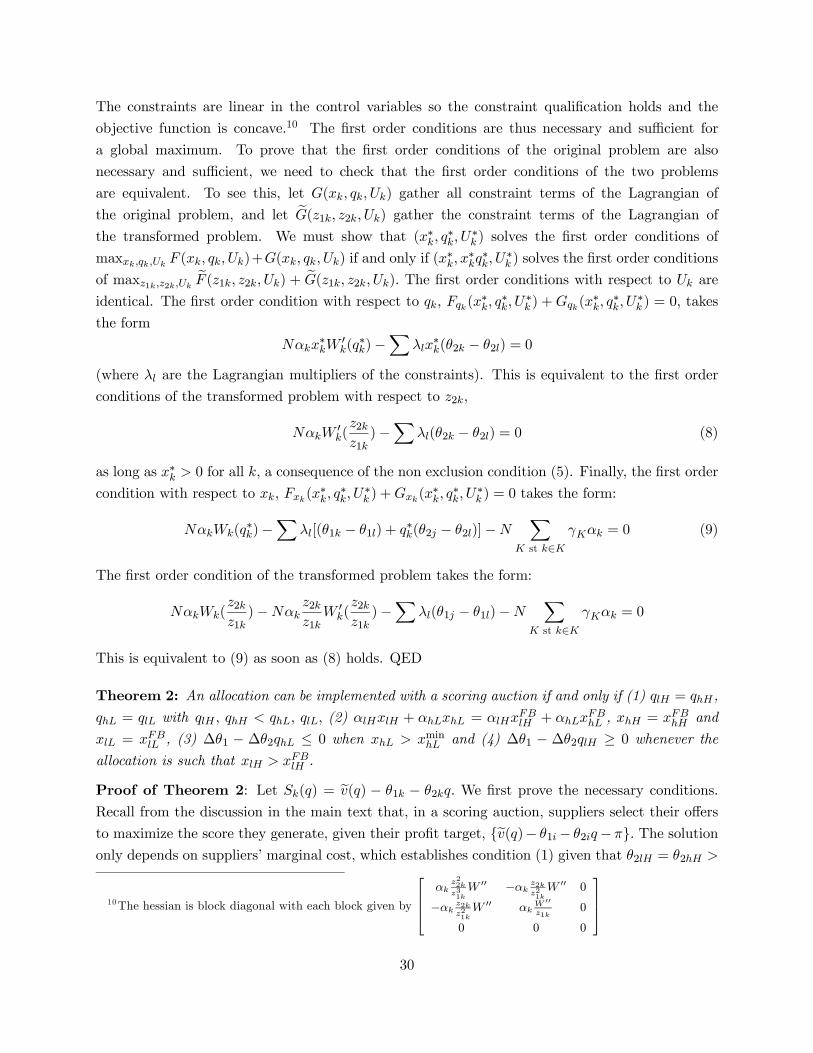
The constraints are linear in the control variables so the constraint qualification holds and the

objective function is concave.10 The first order conditions are thus necessary and sufficient for

a global maximum. To prove that the first order conditions of the original problem are also

necessary and sufficient, we need to check that the first order conditions of the two problems

are equivalent. To see this, let G(xk, qk, Uk) gather all constraint terms of the Lagrangian of

the original problem, and let eG(z1k, z2k, Uk) gather the constraint terms of the Lagrangian of

the transformed problem. We must show that (x∗k, q∗k, U

∗k ) solves the first order conditions of

maxxk,qk,Uk F (xk, qk, Uk)+G(xk, qk, Uk) if and only if (x∗k, x∗kq∗k, U

∗k ) solves the first order conditions

of maxz1k,z2k,Uk eF (z1k, z2k, Uk) + eG(z1k, z2k, Uk). The first order conditions with respect to Uk are

identical. The first order condition with respect to qk, Fqk(x∗k, q

∗k, U

∗k ) +Gqk(x

∗k, q

∗k, U

∗k ) = 0, takes

the form

Nαkx∗kW

0k(q

∗k)−

Xλlx

∗k(θ2k − θ2l) = 0

(where λl are the Lagrangian multipliers of the constraints). This is equivalent to the first order

conditions of the transformed problem with respect to z2k,

NαkW0k(z2kz1k)−

Xλl(θ2k − θ2l) = 0 (8)

as long as x∗k > 0 for all k, a consequence of the non exclusion condition (5). Finally, the first order

condition with respect to xk, Fxk(x∗k, q

∗k, U

∗k ) +Gxk(x

∗k, q

∗k, U

∗k ) = 0 takes the form:

NαkWk(q∗k)−

Xλl[(θ1k − θ1l) + q∗k(θ2j − θ2l)]−N

XK st k∈K

γKαk = 0 (9)

The first order condition of the transformed problem takes the form:

NαkWk(z2kz1k)−Nαk

z2kz1k

W 0k(z2kz1k)−

Xλl(θ1j − θ1l)−N

XK st k∈K

γKαk = 0

This is equivalent to (9) as soon as (8) holds. QED

Theorem 2: An allocation can be implemented with a scoring auction if and only if (1) qlH = qhH ,

qhL = qlL with qlH , qhH < qhL, qlL, (2) αlHxlH + αhLxhL = αlHxFBlH + αhLx

FBhL , xhH = xFBhH and

xlL = xFBlL , (3) ∆θ1 − ∆θ2qhL ≤ 0 when xhL > xminhL and (4) ∆θ1 − ∆θ2qlH ≥ 0 whenever the

allocation is such that xlH > xFBlH .

Proof of Theorem 2: Let Sk(q) = ev(q) − θ1k − θ2kq. We first prove the necessary conditions.

Recall from the discussion in the main text that, in a scoring auction, suppliers select their offers

to maximize the score they generate, given their profit target, {ev(q)− θ1i− θ2iq−π}. The solutiononly depends on suppliers’ marginal cost, which establishes condition (1) given that θ2lH = θ2hH >

10The hessian is block diagonal with each block given by

⎡⎢⎢⎣αk

z22kz31kW 00 −αk z2kz2

1kW 00 0

−αk z2kz21kW 00 αk

W 00

z1k0

0 0 0

⎤⎥⎥⎦30

θ2hL = θ2lL. Condition (2) follows from the fact that lL can always generate a strictly higher score

than either lH and hL for all choices of the scoring rule ev(.). Similarly, both lH and hL can always

generate a strictly higher score than hH so they must win against a hH type.

When xhL > xminhL , ShL(qhL) ≥ SlH(qlH), or else lH should have priority over hL in the allocation.

This implies that

ev(qhL)− h− LqhL ≥ ev(qlH)− l −HqlH , that is,

∆θ1 −∆θ2qhL ≤ ev(qhL)− ev(qlH)−H(qhL − qlH)

In addition, incentive compatibility requires that lH generates a higher score by choosing qlH than

qhL, i.e. ev(qhL)− ev(qlH)−H(qhL − qlH) ≤ 0

Combining both inequalities yields condition (3). Similarly, when xlH > xFBlH , SlH(qlH) ≥ ShL(qhL),

else hL should have priority in the allocation. This implies ∆θ1−∆θ2qlH +L(qhL− qlH)+ev(qlH)−ev(qhL) ≥ 0. In addition, hL must be generating a higher score by choosing qhL over qlH , i.e.

L(qhL − qlH) + ev(qlH)− ev(qhL) ≤ 0. Combining both inequalities yields condition (4).To prove sufficiency, we construct a scoring rule that implements the intended allocation in a

second-score auction (in a second-score auction, it is a dominant strategy to submit bids generating

scores Sk(qk) = maxq{ev(q)− θ1k − θ2kq}). Consider

ev(q) = υ(q)1{q≤qlH} + υ(qlH)1{q>qlH} + 1{q≥qhL}

For this scoring auction to implement the outcome, two conditions must be satisfied. First, suppliers

must be choosing the assigned qualities when they maximize their scores. Second, the ranking of

the scores must (weakly) correspond to the assigned ranking of types in the allocation.

Given the shape of this scoring rule, the two relevant choices are qlH and qhL. lH prefers qlH to qhLif and only if υ(qlH)− l−HqlH ≥ υ(qlH)+ε− l−HqhL i.e. ε ≤ H(qhL−qlH) (hH’s preferences yieldthe same condition). hL prefers qhL to qlH if and only if υ(qlH)+ε−h−LqhL ≥ υ(qlH)−h−LqlH ,i.e. ε ≥ L(qhL − qlH) (lL’s preferences yield the same condition). Hence, suppliers choose their

assigned qualities if ε satisfies the following inequalities:

L(qhL − qlH) ≤ ε ≤ H(qhL − qlH), (10)

which is possible by condition (1). Next, hL generates a higher score if and only if ShL(qhL) =

υ(qlH) + ε− h− LqhL ≥ SlH(qlH) = υ(qlH)− l −HqlH i.e.

ε ≥ ∆θ1 −HqlH + LqhL = ∆θ1 −∆θ2qhL +H(qhL − qlH) (11)

lH generates a higher score otherwise. Inequalities (10) and (11) are always compatible if ∆θ1 −∆θ2qhL ≤ 0 holds. When the solution is such that xlH > xFBlH , we need SlH(qlH) ≥ ShL(qhL) :

ε ≤ ∆θ1 −HqlH + LqhL = ∆θ1 −∆θ2qlH + L(qhL − qlH)

31

instead. It is compatible with (10) if ∆θ1 −∆θ2qlH ≥ 0. Q.E.D.

Theorem 3 (characterization of the optimal sequential procedure): The optimal sequentialprocedure is such that the buyer offers the menu of contracts defined in Lemma 6 in the last round

and, when n > 1, one of the four following pairs of contracts, depending on which one yields the

largest continuation value (conditional on the condition in the third column being satisfied):

Kn Offers (pn1 , qn1 ) and (p

n2 , q

n2 ) Vn

lL (θ1+θ2q,q) αlLWFBlL +(1− αlL)V n−1

lL,lH (θ1+θ2q∗1, q

∗1) αlL(W

FBlL −∆θ2q∗1)+

(θ1+θ2q+∆θ2q∗1,q) αlHWlH(q

∗1) + (αhL+αhH)V n−1

q∗1=argmax {v(q)−θ2q− αlLαlH∆θ2q} Condition: ∆θ1 −∆θ2q∗1 ≥ 0

lL,hL (θ1+θ2q,q) (αlL+αhL)WFBhL +(αlH+αhH)V n−1

lL,lH,hL (θ1+θ2q∗∗1 , q∗∗1 ) (αlL+αhL)(W

FBlL −∆θ2q1)

(θ1+θ2q+∆θ2q∗∗1 ,q) αlHWlH(q

∗∗1 ) + αhHVn−1

q∗∗1 =argmax {v(q)−θ2q−(αlL+αhL)

αlH∆θ2q} Condition: ∆θ1 −∆θ2q∗∗1 ≤ 0

(The first column in the table indicates the set of supplier types who will accept the buyer’s offer when n

suppliers remain, and the third column indicates the buyer’s continuation value, Vn).

(Suppliers of types lH and hH accept the contract (pn1 , qn1 ) if it satisfies their IR constraint, and

likewise, suppliers of types lL and hL accept contract (pn2 , qn2 ) if it satisfies their IR constraint).

Proof: Since suppliers are only made an offer once, they accept this offer whenever it contains acontract that satisfies their IR constraint. By design, the contracts will be such that (pn1 , q

n1 ) (resp.

(pn2 , qn2 )) is the contract chosen by the high (resp. low) marginal cost suppliers.

Let Kn be the set of supplier types who accept one of the offers when n suppliers remain. Given

suppliers’ cost structure, Kn ∈ {{lL}, {lL, lH}, {lL, hL}, {lL, lH, hL}, {lH, hH, hL, lL}}. We firstargue that Kn 6= {lH, hH, hL, lL}, for n > 1, i.e. some exclusion is optimal. By offering the single

contract (θ1 + θ2q, q) that excludes all suppliers but lL, and the last round contract forever after

(Lemma 6), the buyer guarantees himself an expected utility of αlLWFBlL + (αlH + αhH + αhL)V1

> V1, his continuation value if Kn = {lH, hH, hL, lL}. We now examine the optimal offers for theother three inclusion sets.

Kn = {lH, lL}: lH’s IR constraint is binding, p1 = θ1 + θ2q1 and lL’s IC constraint is binding,

p2 = p1−θ2q1+θ2q2. The optimal qualities solve αlH(v(q1)−θ1−θ2q1)+ αlL(v(q2)−θ1−Lq2−∆θ2q1),thus q∗1 = argmax{v(q)− θ2q− αlL

αlH∆θ2q}. For this solution to be feasible we need in addition that

hL is indeed excluded, i.e. that p1 − θ1 − θ2q∗1 ≤ 0, i.e. ∆θ1 −∆θ2q∗1 ≥ 0.

Kn = {hL, lL}: Only one contract is offered in this case: (θ1 + θ2q, q). For this solution to be

feasible, lH’s IR constraint must be violated, i.e. ∆θ1−∆θ2q ≤ 0, which is automatically satisfiedin our model.

32

Kn = {lH, hL, lL}: As before the binding IC constraint is from lL and hL to lH (this will hold

as long as q1 ≤ q2), hence p2 − θ2q2 = p1 − θ2q1. We need to distinguish between two scenarios

depending on which, from lH or hL’s IR constraints, is binding. Case 1: lH’s IR constraint is

binding at the optimum, i.e., p1 = θ1 + θ2q1. Substituting into the buyer’s utility function, the

resulting qualities solve αlH(v(q1)− θ1 − θ2q1)+ (αhL + αlL)(v(q2)− θ1 − θ2q2 −∆θ2q1). The lastcondition to check is that hL’s IR constraint is indeed satisfied i.e. ∆θ1 − ∆θ2q∗∗1 ≤ 0. Case 2:hL’s IR constraint is binding at the optimum, i.e. p2 = θ1 + θ2q2. Hence the resulting qualities

must solve αlH(v(q1)− θ1 − θ2q1)+ (αhL + αlL)(v(q2)− θ1 − θ2q2), that is, q1 = q2 = q : the buyer

offers a single contract. lH’s IR constraint is satisfied if ∆θ1 − ∆θ2q ≥ 0. (This is ruled out byassumption). Q.E.D.

33

Table 1: Probabilities of winning and quality levels when ∆θ1 −∆θ2q ≥ 0Solution Probabilities of Winning qlL qhL qlH qhH

Condition: xFBhH [∆θ1 −∆θ2q2hH ] ≤ xFBlH [∆θ1 −∆θ2q]1.1.a xk = xFBk q q q q2hH1.1.b xlL = xFBlL > xlH = xmaxlH > xhL = xminhL > xhH = xFBhH q q q q2hH1.1.c xlL = xFBlL > xmaxlH ≥ xlH > xhL ≥ xminhL > xhH = xFBhH q q (q2lH , q) (q2hH , q)

1.1.d xlL = xFBlL > xlH = xmaxlH > xminhL = xhL > xhH > xFBhH q q (q2lH , q) (q2hH , q)

1.1.e xlL = xFBlL > xlH > xhL = xhH > xFBhH q q (q2lH , qhH) (q2hH , q)

Condition: xFBhH [∆θ1 −∆θ2q2hH ] > xFBlH [∆θ1 −∆θ2q]1.2.a* xk = xFBk q q (q2lH , q) (q2hH , q)

1.2.b* xlL = xFBlL > xFBhL > xhL > xlH > xFBlH > xhH = xFBhH q q (q2lH , q) (q2hH , q)

1.2.c* xlL = xFBlL > xFBhL > xhL = xlH > xFBlH > xhH = xFBhH q q (q2lH , q) (q2hH , q)

Other relevant solutions are 1.1.b, 1.1.c, 1.1.d and 1.1.eAdditional conditions as well as exact values for the variables in the individual solutions are available in Asker and Cantillon (2005)

as well as in a separate appendix available on our webpages.

* Under the condition that ∆θ1−∆θ2q≥ 0 we can tighten the bound on qhH so that qhH ∈ (q2hH , qlH)

Table 2: Probabilities of winning and quality levels when ∆θ1 −∆θ2q < 0Solution Probabilities of Winning (x’s) qlL qhL qlH qhH

Condition: xFBhH [∆θ1 −∆θ2q] ≥ xFBlH [∆θ1 −∆θ2q2lH ]2.1.a xk = xFBk q q q2lH q

2.1.b xlL = xFBlL > xFBhL > xhL = xlH > xFBlH > xhH = xFBhH q q q2lH q

2.1.c xlL = xFBlL > xhL = xFBhL > xFBlH > xlH > xhH > xFBhH q q (q2lH , qhH) (q2hH , q)

2.1.d xlL = xFBlL > xFBhL > xlH = xhL > xFBlH > xhH > xFBhH q q (q2lH , qhH) (q2hH , q)

2.1.e xlL = xFBlL > xlH > xhL = xhH > xFBhH q q (q2lH , qhH) (q2hH , q)

Condition: xFBhH [∆θ1 −∆θ2q] < xFBlH [∆θ1 −∆θ2q2lH ]The relevant solutions are 1.2.a, 1.2.b, 1.2.c, 2.1.c, 2.1.d and 2.1.eAdditional conditions as well as exact values for the variables in the individual solutions are available in Asker and Cantillon (2005)

as well as in a separate appendix available on our webpages.

34

lH

lL hL

hH lH

lL(a) (b)

q21 θθ ∆>∆ q21 θθ ∆<∆

Figure 1: binding constraints in the efficient auction

lH

lL hL

hH lH

lL hL

hH lH

lL hL

hH lH

lL hL

hH

1.1.a

1.1.b

1.1.c

1.1.d

1.2.a

1.2.b

1.2.c

lH

hL

hH

1.1.elL

Figure 2: Binding IC constraints at the solution when ∆θ1 −∆θ2q ≥ 0

lH

lL hL

hH lH

lL hL

hH lH

lL hL

hH lH

lL hL

hH

2.1.a 2.1.b 2.1.c

1.2.a

1.2.b

2.1.d

1.2.c

lH

hL

hH

2.1.elL

Figure 3: Binding IC constraints at the solution when ∆θ1 −∆θ2q < 0

35

Revenue by MechanismProbabilities: Pr(lH) = 25, Pr(hH)= 25, Pr(hL)= 25, Pr(lL)= 25

0

0.1

0.2

0.3

0.4

0.5

0.00001 0.1125 0.225 0.3375 0.45 0.5625 0.675 0.7875 0.9 1.0125 1.125

Expe

cted

Rev

enue

per

Bid

der

Efficient Auction

Optimal Scoring Auction

Optimal Mechanism

Figure 4

Figure 5: Proportion of (Optimal - Efficient Auction)

Probabilities: Pr(lH) = 25, Pr(hH)= 25, Pr(hL)= 25, Pr(lL)= 25

0

0.1

0.2

0.3

0.4

0.5

0.6

0.7

0.8

0.9

1

0.00001 0.1125 0.225 0.3375 0.45 0.5625 0.675 0.7875 0.9 1.0125 1.125

%

Probabilities: Pr(lH) = 15, Pr(hH)= 35, Pr(hL)= 15, Pr(lL)= 35

0

0.1

0.2

0.3

0.4

0.5

0.6

0.7

0.8

0.9

1

0.00001 0.1125 0.225 0.3375 0.45 0.5625 0.675 0.7875 0.9 1.0125 1.125

%

Probabilities: Pr(lH) = 35, Pr(hH)= 15, Pr(hL)= 35, Pr(lL)= 15

0

0.1

0.2

0.3

0.4

0.5

0.6

0.7

0.8

0.9

1

0.00001 0.1125 0.225 0.3375 0.45 0.5625 0.675 0.7875 0.9 1.0125 1.125

%

Probabilities: Pr(lH) = 35, Pr(hH)= 35, Pr(hL)= 15, Pr(lL)= 15

0

0.1

0.2

0.3

0.4

0.5

0.6

0.7

0.8

0.9

1

0.00001 0.1125 0.225 0.3375 0.45 0.5625 0.675 0.7875 0.9 1.0125 1.125

%

1θ∆

1θ∆1θ∆

1θ∆

36

Table 3: Proportion of the (opt. mech. - efficient auction) expected utility captured by the optimal scoring auction

Probabilities Average Max ∆θ1 at Min ∆θ1 at % of ∆θ1’s such that proportion is:

maximum minimum >80% of opt. mech. < minimum +0.1

Core Parameter Values

1 25 25 25 25 0.825 1.00 0.248 0.389 0.585 74.1 4.5

2 20 30 20 30 0.874 1.00 0.248 0.739 0.574 86.6 19.4

3 15 35 15 35 0.901 1.00 0.248 0.756 0.000 97.5 7.0

4 30 20 30 20 0.761 1.00 0.248 0.284 0.686 62.2 13.4

5 35 15 35 15 0.685 1.00 0.248 0.191 0.799 52.7 22.4

6 20 20 30 30 0.812 1.00 0.180 0.423 0.596 68.2 5.0

7 15 15 35 35 0.796 1.00 0.124 0.449 0.630 47.3 7.0

8 30 30 20 20 0.835 1.00 0.315 0.372 0.574 74.1 3.5

9 35 15 15 35 0.839 1.00 0.383 0.376 0.563 75.6 3.5

10 20 30 30 20 0.779 1.00 0.248 0.465 0.709 44.8 14.9

11 15 35 35 15 0.778 1.00 0.248 0.558 0.833 41.3 26.9

12 30 20 20 30 0.892 1.00 0.248 0.670 0.518 83.6 13.4

13 35 15 15 35 0.948 1.00 0.248 0.809 0.000 100 20.4

Extensions

14 10 40 10 40 0.823 1.00 0.248 0.593 1.125 56.7 25.8

15 40 10 40 10 0.604 1.00 0.248 0.127 0.810 45.7 31.8

16 10 10 40 40 0.786 1.00 0.068 0.442 0.698 40.8 6.5

17 40 40 10 10 0.836 1.00 0.450 0.358 0.563 60.2 4.5

18 45 45 5 5 0.826 1.00 0.506 0.209 0.000 50.2 2.0

19 15 25 30 30 0.817 1.00 0.153 0.535 0.038 51.2 7.5

20 16 23 41 20 0.752 1.00 0.180 0.463 0.821 39.3 13.4

Robustness: a = 1

21 25 25 25 25 0.825 1.00 0.028 0.389 0.065 74.1 4.5

22 15 35 15 35 0.901 1.00 0.028 0.756 0.000 97.5 7.0

23 35 15 35 15 0.685 1.00 0.028 0.191 0.088 52.7 22.4

24 15 15 35 35 0.796 1.00 0.014 0.449 0.070 47.3 7.0

25 35 35 15 15 0.839 1.00 0.043 0.376 0.063 75.6 3.5

Robustness: b = 0.7

26 25 25 25 25 0.737 1.00 0.285 0.429 2.078 49.3 24.9

Robustness: ∆θ2 = 2

27 25 25 25 25 0.751 1.00 0.180 0.409 0.765 53.2 19.9

Robustness: l = 2

38 25 25 25 25 0.827 1.00 0.248 0.389 0.585 74.6 4.0

Notes: Each experiments sets the probabilites of each type (ordered αlH , αhH , αhL, αlL), then computes the expected

utility for the optimal mechanism, the efficient auction and the optimal scoring auction for 201 values of ∆θ1 covering

the full range of the parameter values allowed by the model.

.

Table 4: Percentage of the (optimal mechanism - efficient auction) expected utility

captured by the simple scoring rule corresponding to an adjusted efficient auction

Probabilities Average No Distortion to Allocation Distortion to Allocation

Max Min Max Min

a∗ = (0.95) a

1 25 25 25 25 0.223 38.3 -19.5 78.1 72.9

2 20 30 20 30 0.225 39.8 -7.8 76.5 71.2

3 15 35 15 35 0.218 36.6 -1.6 71.9 68.5

4 30 20 30 20 0.237 36.3 -32.3 79.3 63.1

5 35 15 35 15 0.242 34.0 -49.3 80.5 38.0

6 20 20 30 30 0.286 30.0 -20.4 73.8 66.1

7 15 15 35 35 0.339 20.5 -25.5 68.7 58.7

8 30 30 20 20 0.174 46.4 -23.3 81.9 79.2

9 35 15 15 35 0.114 53.8 -37.9 85.0 84.4

10 20 30 30 20 0.208 40.2 -10.5 68.6 56.3

11 15 35 35 15 0.186 41.9 -2.6 55.5 33.8

12 30 20 20 30 0.254 35.8 -19.7 85.5 76.5

13 35 15 15 35 0.277 25.0 -17.4 88.5 79.0

a∗ = (0.9) a

1 25 25 25 25 0.195 36.2 1.4 82.3 80.6

2 20 30 20 30 0.194 32.1 2.2 80.2 78.2

3 15 35 15 35 0.189 28.3 3.3 75.1 74.6

4 30 20 30 20 0.187 36.3 0.5 84.3 75.4

5 35 15 35 15 0.170 36.8 -3.4 81.8 69.2

6 20 20 30 30 0.170 29.6 1.0 78.5 76.0

7 15 15 35 35 0.145 23.8 0.3 74.8 71.5

8 30 30 20 20 0.222 44.2 1.5 86.1 85.4

9 35 35 15 15 0.253 54.6 1.4 90.3 89.8

10 20 30 30 20 0.199 36.2 3.2 73.2 68.9

11 15 35 35 15 0.200 36.3 6.3 60.7 52.9

12 30 20 20 30 0.185 29.6 0.3 88.3 81.6

13 35 15 15 35 0.170 21.4 -1.2 87.0 82.4

38

Table 5: Contracts in the optimal sequential procedureKn Offers (pn1 , q

n1 ) and (p

n2 , q

n2 ) Vn

lL (θ1+θ2q,q) αlLWFBlL +(1− αlL)V n−1

lL,lH (θ1+θ2q∗1, q

∗1) αlL(W

FBlL −∆θ2q∗1)+

(θ1+θ2q+∆θ2q∗1,q) αlHWlH(q

∗1) + (αhL+αhH)V n−1

q∗1=argmax {v(q)−θ2q− αlLαlH∆θ2q} Condition: ∆θ1 −∆θ2q∗1 ≥ 0

lL,hL (θ1+θ2q,q) (αlL+αhL)WFBhL +(αlH+αhH)V n−1

lL,lH,hL (θ1+θ2q∗∗1 , q∗∗1 ) (αlL+αhL)(W

FBlL −∆θ2q1)

(θ1+θ2q+∆θ2q∗∗1 ,q) αlHWlH(q

∗∗1 ) + αhHVn−1

q∗∗1 =argmax {v(q)−θ2q−(αlL+αhL)

αlH∆θ2q} Condition: ∆θ1 −∆θ2q∗∗1 ≤ 0

(The first column in the table indicates the set of supplier types who will accept the buyer’s offer when n

suppliers remain, and the third column indicates the buyer’s continuation value, Vn).

Table 6: Virtual welfares and probabilities in the efficient auction

Virtual welfares Probabilities

∆θ1 −∆θ2q > 0 ∆θ1 −∆θ2q < 0 pk = NαkxFBk

WFBlL WFB

lL 1− (1− αlL)2

WFBhL −

αlLαhL∆θ1 WFB

hL −αlLαhL∆θ1 (1− αlL)

2−(1− αlL−αhL)2

WFBlH WFB

lH +αlL+αhLαlH

∆θ1−αlL+αhLαlH

∆θ2q (1− αlL−αhL)2−(1− αlL−αhL−αlH)

2

WFBB − αlH

αhH∆θ1−αhL+αlL

αhHq WFB

hH −αlH+αhL+αlL

αhH∆θ1 α2hH

39

Probabilities: Pr(lH) =25, Pr(hH)=25, Pr(hL)=25, Pr(lL)=25, a*= (0.95)a

0

0.1

0.2

0.3

0.4

0.5

0.6

0.7

0.8

0.9

1

0.00001 0.1125 0.225 0.3375 0.45 0.5625 0.675 0.7875 0.9 1.0125 1.125

%

Optimal scoring auction

Naïve scoring auction

Probabilities: Pr(lH) =25, Pr(hH)=25, Pr(hL)=25, Pr(lL)=25, a*= (0.95)a

0

0.1

0.2

0.3

0.4

0.5

0.6

0.7

0.8

0.9

1

0.00001 0.1125 0.225 0.3375 0.45 0.5625 0.675 0.7875 0.9 1.0125 1.125

%

Optimal scoring auction

Naïve scoring auction

Figure 6: Performance of nave scoring auctions

.

0

0.1

0.2

0.3

0.4

0.5

0.6

0.7

0.8

0.9

1

1E-05 0.0

45 0.09

0.135 0.1

80.2

25 0.27

0.315 0.3

60.4

05 0.45

0.495 0.5

40.5

85 0.63

0.675 0.7

20.7

65 0.81

0.855 0.9

0.945 0.9

91.0

35 1.08

1.125

EFFICIENT

SEQUENTIAL

Figure 7: Performance of the optimal sequential procedure and the efficient auction for different values of

∆θ1 when v(q) = 3√q, θ1 = θ2 = 1, θ2 = 2, αlH = αhL = 0.35 and αlL = αhH = 0.15

39

Table 7: Proportion of the (optimal mechanism - efficient auction) expected utility captured by the

optimal sequential procedure∗

Probabilities Average Max ∆θ1 Min ∆θ1 % ∆θ1 % ∆θ1

at max at min s.t. >80% s.t. >0%

1 25 25 25 25 -152.7% 100% 0 -504.4% 0.5625 6.9 20.8

2 20 30 20 30 -78.2% 100% 0 -279.6% 0.5625 7.9 23.8

3 15 35 15 35 -7.2% 100% 0 -83.6% 0.5625 7.9 35.6

4 10 40 10 40 55.9% 100% 0 39.2% 0.5625 8.9 100

5 30 20 30 20 -238.7% 100% 0 -663.9% 0.66375 5.9 18.8

6 35 15 35 15 -365.0% 100% 0 -942.2% 0.7875 5.0 15.8

7 40 10 40 10 -591.8% 100% 0 -1,446.7% 0.9 5.0 13.9

8 20 20 30 30 -126.4% 100% 0 -404.0% 0.5625 5.9 22.8

9 15 15 35 35 -107.6% 100% 0 -356.2% 0.5625 5.9 21.8

10 10 10 40 40 -95.5% 100% 0 -284.4% 0.5625 5.0 18.8

11 30 30 20 20 -198.6% 100% 0 -746.5% 0.5625 6.9 18.8

12 35 35 15 15 -280.2% 100% 0 -1.302.9% 0.5625 6.9 14.9

13 40 40 10 10 -394.1% 100% 0 -1,961.4% 0.5625 6.0 9.9

14 20 30 30 20 -147.2% 100% 0 -384.1% 0.66375 7.9 25.7

15 15 35 35 15 -108.2% 100% 0 -276.6% 0.7875 10.9 32.7

16 10 40 40 10 -46.1% 100% 0 -164.7% 0.9 15.8 40.6

17 30 20 20 30 -129.3% 100% 0 -411.4% 0.5625 5.9 16.8

18 35 15 15 35 -93.9% 100% 0 -244.8% 0.5625 5.0 13.9

19 40 10 10 40 -61.4% 100% 0 -142.% 0.5625 4.0 13.9∗Each experiment sets the value of the αk’s (ordered αlH , αhH , αhL, αlL) and computes the expected utilityfrom the optimal mechanism, the optimal sequential auction and the efficient auction for all the values for∆θ1 allowed by the model. Each experiment samples 101 equally spaced values for ∆θ1

40

Appendix Z: Full Proofs

(Not for publication)

Not For Publication

Appendix Z: Proof of Theorem 1

Set-up of the Optimal Program

For future reference, this appendix reproduces the optimization problem of the buyer with UhH = 0

(Lemma 2) and with the subset of the IC constraints that happen to bind at the optimum.

max{xk,qk,Uk}

αlH [xlHWlH(qlH)− UlH ]+αhHxhHWhH(qhH)+αhL [xhLWhL(qhL)− UhL]+αlL [xlLWlL(qlL)− UlL]

subject to:

UlH ≥ xhH∆θ1 (IC 1)

UhL ≥ UlH − xlH [WlH (qlH)−WhL (qlH)] (IC 2)

UhL ≥ xhHqhH∆θ2 (IC 3)

UlL ≥ UlH + xlHqlH∆θ2 (IC 4)

UlL ≥ UhL + xhL∆θ1 (IC 5)

UlL ≥ UhH + xhH∆θ1 + xhHqhH∆θ2 (IC 6)

NPk∈K

αkxk ≤ 1− (1−Pk∈K

αk)N for all subsets K of {lH, hH, hL, lL} (feasibility)

(We omit the non exclusion constraint). The associated Lagrangian is given by:

αlH [xlHWlH(qlH)− UlH ] + αhHxhHWhH(qhH) + αhL [xhLWhL(qhL)− UhL] + αlL [xlLWlL(qlL)− UlL](1)

+λ1 [UlH − xhH∆θ1] + λ2 [UhL − UlH + xlH (WlH (qlH)−WhL (qlH))]

+λ3 [UhL − xhHqhH∆θ2] + λ4 [UlL − UlH − xlHqlH∆θ2] + λ5 [UlL − UhL − xhL∆θ1]

λ6 [UlL − xhH∆θ1 − xhHqhH∆θ2]−P

γK

∙NPk∈K

αkxk − 1 + (1−Pk∈K

αk)N

¸(where λi is the Lagrangian multiplier associated with IC constraint i, and γK is the multiplier

associated with feasibility constraint K). Figure 13 provides a graphical representation of these IC

constraints together with their associated multipliers. A dotted line means that a constraint may

bind at the optimum. A full line means it always binds.

λ3

lH hH

hLlL λ5

λ4

λ6

λ2

λ1

λ3

lH hH

hLlL λ5

λ4

λ6

λ2

λ1

Figure 13: Potentially binding constraints at the solution

42

Not For Publication

The Kuhn-Tucker conditions of this program are standard. For future reference, we only reproduce

those with respect to Uk :

λ1 − λ2 − λ4 = αlH (2)

λ2 + λ3 − λ5 = αhL (3)

λ4 + λ5 + λ6 = αlL (4)

Characterization of the Optimal Buying Mechanism

Preliminaries

We first define the notation that we will be using for some of the xk variables when they take

specific values. When xlH takes its maximum value conditional on lL keeping priority in the

contract allocation, we will denote it xmaxlH . Formally, xmaxlH is defined by the equation

N¡αlHx

maxlH + αlLx

FBlL

¢= 1− (αhL + αhH)

N

By Border (1991), this implies the following allocation: When there is a type lL, give the contract

to lL, if not, give priority to a type lH if there is one. Conversely, xminhL corresponds to the expected

probability of winning for hL when lH and lL have priority over hL (but hL maintains priority

over hH). Formally,

N¡αlHx

maxlH + αhLx

minhL + αlLx

FBlL

¢= 1− αNhH

Finally, x is defined such that xlH = xhL and they have priority over hH in the allocation, that is

N¡(αlH + αhL)x+ αlLx

FBlL

¢= 1− αNhH

The proof of Theorem 1 uses the following result repeatedly:

Lemma 7: Suppose UlH = xhH∆θ1. (1) Suppose further that UhL,lH ≥ UhL,hH . Then, xhL > xlH

if and only if UlL,hL > UlL,lH . (2) Suppose now that UhL,lH ≤ UhL,hH . Then UlL,hL ≥ UlL,lH when

xhL ≥ xlH .

Proof: The result follows directly from a comparison of UlL,lH and UlL,hL (when UhL,lH ≥ UhL,hH) :

UlL,lH = xlHqlH∆θ2 + xhH∆θ1 UlL,hL = xhL∆θ1 − xlH∆θ1 + xlHqlH∆θ2 + xhH∆θ1

When UhL,hH ≥ UhL,lH , UlL,hL = xhL∆θ1 + xhHqhH∆θ2. Since UhL,hH ≥ UhL,lH is equivalent to

xhH [WlH(qhH) −WhL(qhH)] ≤ xlH [WlH(qlH) −WhL(qlH)], the condition implies UlL,hL ≥ UlL,lH

when xhL > xlH . QED.

43

Not For Publication

Lemma 8: Suppose that IC hL,hH is satisfied. Then xhL ≥ xhH =⇒ IC lL,hH is satisfied.

Proof: IChL,hH satisfied means that UlL,hLdefn= UhL + xhL∆θ1 ≥ UhH + xhH∆θ2qhH + xhL∆θ1.

On this other hand, UlL,hH = UhH + xhH∆θ2qhH + xhH∆θ1. Clearly, UlL,hH ≤ UlL,hL as long as

xhL ≥ xhH . QED

We are now ready to prove theorem 1. The proof proceeds by progressively partioning the space of

parameters into sets of parameters for which the solution shares the same binding IC and feasibility

constraints. The logic of the proof is pretty simple, even if the mechanics can be involved. For this

reason an exhaustive exposition of the proof of part I, scenario 1 is presented. The arguments in

the rest of the proof are presented more briefly where they mirror those in part I, scenario 1.

Proof of part I of Theorem 1: WlH (q)−WhL (q) > 0 i.e. ∆θ1 > q∆θ2

The binding constraints in the buyer-optimal efficient mechanism are IClH,hH , IChL,hH and IClL,hL.

The buyer’s resulting expected utility is given by

αlHxlHWlH(qlH) + αhHxhH [WhH(qhH)−αlHαhH

∆θ1 −αhL + αlL

αhHqhH∆θ2] (5)

+αhLxhL[WhL(qhL)−αlLαhL∆θ1] + αlLxlLWlL(qlL)

(where, again, we have highlighted the virtual welfares associated with each type). Keeping the

probabilities fixed at xk = xFBk , optimizing the q’s in (5) requires that only qhH be adjusted away

from the efficient level and set equal to

q2hH = argmax{WhH(qhH)−αlHαhH

∆θ1 −αhL + αlL

αhHqhH∆θ2} (6)

This reduces the informational rents of hL and lL. From Lemma 7(2), we know that UlL,hL ≥ UlL,lH

as long as UhL,hH ≥ UhL,lH . Hence, we need to consider only two scenarios:

Scenario 1: At q2hH , UhL,hH ≥ UhL,lH , that is,

xFBhH [WlH(q2hH)−WhL(q

2hH)] ≤ xFBlH [WlH(q)−WhL(q)] (7)

In this case, all IC constraints remain satisfied as we decrease qhH to q2hH .

We now consider the optimization of the probabilities of winning. From (5) and the model assump-

tions, the virtual welfare associated with lL is the largest. Moreover, the virtual welfare associated

with lH is larger than that associated with hH. Thus, we need to consider three cases depending

on the relative ranking of the virtual welfare of hL with respect to the virtual welfares of hH and

lH.

44

Not For Publication

1. VWhL ≥ VWlH ≥ VWhH :WhL(q)− αlLαhL∆θ1 ≥WlH(q) > WhH(q

2hH)−

αlHαhH∆θ1−αhL+αlL

αhHq2hH∆θ2

[Solution 1.1.a]

The optimal probabilities of winning are xk = xFBk since the ranking of the virtual welfares

corresponds to the ranking of the first best welfares. All IC constraints are satisfied given

the arguments above. The x’s and q’s are optimized given the binding constraints; qlH = q,

qhH = q2hH and qhL = qlL = q.

2. VWlH > VWhL ≥ VWhH :WlH(q) > WhL(q)− αlLαhL∆θ1 ≥WhH(q

2hH)−

αlHαhH∆θ1−αhL+αlL

αhHq2hH∆θ2

In this case, type lH generates a higher level of virtual welfare than type hL. Thus, the

buyer would rather give the contract to supplier lH than to supplier hL, i.e. he would

like to change the order of priority in the allocation. Increasing xlH while decreasing xhL

concurrently (keeping αlHxlH + αhLxhL + αlLxFBlL constant) does not initially affect any of

the virtual welfare and it increases the buyer’s expected utility. This process continues until

either a new IC constraint binds or we have reach xlH = xmaxlH .

We now argue that the only potentially new binding constraint is IClL,lH . To see this consider

the following:

(a) hL’s IC constraints: Given that UhL,lH = UlH − xlH [∆θ1 − ∆θ2q] and that UlH is not

affected by the process, the incentives for hL to imitate lH have actually decreased.

IChL,lL remain satisfied as well since IClL,hL is binding and xlL > xhL.

(b) lH’s IC constraints: Because UlH,hL = UhL + xhL(∆θ1 −∆θ2q2hH) and UlH,lL = UhL +

xhL∆θ1 − xlL∆θ2q, the incentives for lH to imitate hL and lL have decreased (UhL =

xhH∆θ1q2hH is not affected by the process).

(c) hH’s IC constraints: hH continues to have no incentive to imitate hH, hL or lL given

that IClH,hH and IChL,hH are binding, and UhH,lL is not affected by the process.

(d) lL’s IC constraint: By Lemma 8, IClL,hH is not affected by the process. By Lemma 7(2),

IClL,lH remains satisfied as long as xlH ≤ xhL, but it could start binding afterwards.

Thus, we continue to increase xlH at the cost of xhL until either xlH = xmaxlH or IClL,lH starts

binding, whichever comes first.

(a) xlH = xmaxlH first. [Solution 1.1.b]

This means that UlL,hL ≥ UlL,lH even when xlH reaches its maximum. This corresponds

to the solution because there are no more opportunities to increase the buyer’s expected

utility: the q’s are optimized given the binding IC constraints, the x’s are optimized

45

Not For Publication

given the virtual welfare and the feasibility constraints. The solution is thus: qlH = q,

qhH = q2hH , qhL = qlL = q and xlL = xFBlL > xlH = xmaxlH > xhL = xminhL > xhH = xFBhH .

By the argument just above, all IC constraints are satisfied.

(b) IClL,lH starts binding. [Solution 1.1.c]

At that point, UlL,lH = UlL,hL, that is, xFBhH [WlH(q2hH)−WhL(q

2hH)] = xhL∆θ1−xlHq∆θ2

(note that by Lemma 7(2), this happens at xlH > xhL).

We now argue that we should be looking for a solution where both IClL,hL and IClL,lH

are binding. Indeed, if only IClL,lH binds, the virtual welfare associated with hL isWFBhL

which is greater than the virtual welfare associated with lH. Thus the buyer would want

to set xhL back to xFBhL , but this would bring us back to the starting point.

Thus the buyer further increases his expected utility by increasing xlH and decreasing

xhL while keeping αlHxlH+αhLxhL+αlLxFBlL constant and xFBhH [WlH(qhH)−WhL(qhH)] =

xhL∆θ1 − xlHq∆θ2. This requires that we adjust qhH (specifically we need to increase

qhH).

A change in qhH corresponds to a change in the value of the Lagrangian multiplier on the

IClL,lH constraint. Using the expressions in (1) to (4), we can rewrite the expressions

for lH and hH’s virtual welfares as follows:

VWlH = maxqlH

{WlH(qlH)−λ4αlH

qlH∆θ2} (8)

VWhH = maxqhH

{WhH(qhH)−αlH + λ4αhH

∆θ1 −αhL + αlL − λ4

αhH∆θ2qhH} (9)

where λ4 is the Lagrangian multiplier on the IClL,lH constraint.

Thus, practically, we increase xlH and decrease xhL concurrently to keep αlHxlH +

αhLxhL + αlLxFBlL constant. This implies a new value for qhH and qlH to ensure that

xFBhH [WlH(qhH)−WhL(qhH)] = xhL∆θ1 − xlHqlH∆θ2. These correspond to a new value

for λ4 through (9). Specifically, λ4 increases.

This process increases the virtual welfare associated with hL, WhL(q)− αlL−λ4αhL

∆θ1, and

decreases the virtual welfare associated with lH and hH (see (8) and (9)).

It continues until we have either reached the upper bound to xlH , xmaxlH , or the virtual

welfares associated with lH and hL become equal:

maxqlH

{WlH(qlH)−λ∗4αlH

qlH∆θ2} =WhL(q)−αlL − λ∗4αhL

∆θ1

whichever comes first. Thus λ4 ∈ (0, λ∗4) ⊂ (0, αlL) as required by (4).This defines the solution: xlL = xFBlL > xmaxlH ≥ xlH > xhL ≥ xminhL > xhH = xFBhH ,

qlL = qhL = q and qlH and qhH defined by (8) and (9), qlH , qhH < q. The x’s are

46

Not For Publication

optimized given the virtual welfares and the feasibility constraints. The q’s are optimized

given the binding constraints.

All IC constraints remain satisfied. The arguments for this are the same as those we made

above, except for IChL,lH , which follows because xFBhH [WlH(qhH)−WhL(qhH)]UlL,hL=UlL,lH

=

xhL∆θ1 − xlHqlH∆θ2 < xlH [WlH(qlH)−WhL(qlH)] when xlH > xhL.

3. VWlH ≥ VWhH > VWhL : WlH(q) > WhH(q2hH) −

αlHαhH∆θ1 − αhL+αlL

αhHq2hH∆θ2 > WhL(q) −

αlLαhL∆θ1.

In this case, the ideal ordering of types in the allocation is lL Â lH Â hH Â hL. The

buyer increases his expected utility by decreasing xhL, first to the benefit of xlH (that is,

keeping αlHxlH+αhLxhL+αlLxFBlL constant), and then to the benefit of xhH (that is, keeping

N(αlHxmaxlH + αhLxhL + αlLx

FBlL + αhHxhH) = 1).

This process initially does not affect any of the virtual welfares until a new IC constraint

binds. By the same arguments as in point 2 above, we can establish that the first binding

constraint is IClL,lH .When it binds xhH [∆θ1−∆θ2q2hH ] = xhL∆θ1−xlH∆θ2q. At this point,

xlH > xhL > xhH (the first inequality comes from Lemma 7(2)).

Once this happens, any further improvement requires that we keep UlL,hL = UlL,lH (otherwise,

if UlL,hL < UlL,lH , IClL,hL ceases to bind, the virtual welfare associated with hL bounces back

to WFBhL and thus we get back to the starting point). We are thus in a similar situation as

in point 2 above. Any further change in the x’s requires some changes in the q’s and thus

in the value of the multiplier on the IC constraints. Using the expressions in (1) to (4), the

resulting virtual welfares associated with lH, hH and hL are:

VWlH = maxqlH

{WlH(qlH)−λ4αlH∆θ2qlH} (10)

VWhH = maxhH{WhH(qhH)−

(αlH + λ4)

αhH∆θ1 −

(αhL + αlL − λ4)

αhH∆θ2qhH} (11)

VWhL =WhL(q)−αlL − λ4αhL

∆θ1 (12)

where λ4 ∈ (0, αlL) is such that UlL,hL = UlL,lH i.e. xhH [WlH(qhH)−WhL(qhH)] = xhL∆θ1−xlHqlH∆θ2 for the current value of xhL (xlH and xhH are well-defined once xhL is defined

given that lH has priority hH is also clear). Practically, a decrease in xhL is associated with

an increase in qhH , a decrease in qlH and an increase in λ4. This decreases VWlH and VWhH

and increases VWhL.

The difference relative to Solution 1.1.c is what ends this process. Here, the process ends

47

Not For Publication

when either a new IC constraint binds or the relative ranking of virtual welfare changes.1

The only new IC constraint that can bind is IClL,hH . This happens at xhL = xhH . Thus we

need to distinguish the following cases depending on which event happens first:

(a) We have reached VWlH ≥ VWhH = VWhL and xlH = xmaxlH . Then this is the solution.

The buyer is indifferent between hH and hL. The qualities are given by the value of

λ4 that solves for VWhH = VWhL in (11) and (12), qlL = qhL = q and xlL = xFBlL ,

xlH = xmaxlH > xminhL ≥ xhL > xhH ≥ xFBhH . [Solution 1.1.d]

(b) We have reached VWlH ≥ VWhH = VWhL at xlH < xmaxlH . Then the buyer can further

increase his expected utility by decreasing xhL and increasing xlH keeping UlL,lH =

UlL,hL. This further decreases VWlH and VWhH and increases VWhL. The process stops

when either VWlH = VWhL or xlH = xmaxlH , whichever comes earlier. At the solution

the q’s are defined from (11) and (12) for the value of λ4 at which the process stops,

qlL = qhL = q and xlL = xFBlL , xmaxlH ≥ xlH > xhL ≥ xminhL and xhH = xFBhH . This

corresponds to Solution 1.1.c. above.

(c) We have reached VWlH = VWhH > VWhL. (note that this implies that qlH < qhL given

(10) and (11)). The buyer further increases his expected utility by decreasing xhL and

adjusting xlH and xhH in a way that preserves VWlH = VWhH and UlL,lH = UlL,hL.2

Thus λ4 is fixed and the virtual welfares are not affected. This process continues until

xhL = xhH (< xlH) at which point UlL,hH starts binding. At this stage we have:

UlL,lH = xhH∆θ1 + xlHqlH∆θ2 = UlL,hH = xhH∆θ1 + xhHqhH∆θ2

= UlL,hL = xhL∆θ1 + xhHqhH∆θ2

Using the expressions in (1) to (4), the virtual welfares are given by

VWlH = maxqlH

{WlH(qlH)−λ4αlH∆θ2qlH} (13)

VWhH = maxqhH

{WhH −αlH + λ4αhH

∆θ1 −αhL + αlL − λ4

αhH∆θ2qhH} (14)

VWhL = WhL(q)−αlL − λ4 − λ6

αhL∆θ1 (15)

where λ4 and λ6 are the multipliers on the IClL,lH and IClL,hH constraint respectively.

1No feasibility constraint binds in the process. Indeed, the only potential feasibility constraint would involve xhH

hitting its maximum but this never occurs before xhH = xhL.2The feasibility constraints on the x’s are N(αlLxFBlL +αlHxlH +αhHxhH) ≤ 1−αNhL and N(αlLx

FBlL +αlHxlH +

αhLxhL + αhHxhH) = 1

48

Not For Publication

There exists a value for λ4 and λ6 such that VWlH = VWhH = VWhL and UlL,lH =

UlL,hL = UlL,hH and N(αlHxlH + αhLxhL + αlLxFBlL + αhHxhH) = 1. Indeed, we have

five equations and five unknowns: λ4, λ6, xlH , xhL and xhH (from (15) and the fact

VWlH = VWhL, we know that αlL−λ4−λ6 > 0, thus αhL+αlL−λ4 in (14) is ensured

to be positive which is required by the non negative constraint on the multipliers).

These values for λ4 and λ6 correspond to the solution. At the solution, xlH > xhH = xhL

(implied by UlL,lH = UlL,hL = UlL,hH), qlH < qhL < q and qhL = qhH = q. The buyer is

indifferent among lH, hH and hL and the x’s are thus optimized. The q’s are optimized

given the binding constraints and the value of the multipliers. No new constraint binds in

the process. The argument for this is identical as the one in point 2, except for IChL,lH ,

which follows because xFBhH [WlH(qhH)−WhL(qhH)]UlL,hL=UlL,lH

= xhL∆θ1 − xlHqlH∆θ2 <

xlH [WlH(qlH)−WhL(qlH)] when xlH > xhL. [Solution 1.1.e]

(d) We have reached xhH = xhL. At this point, IClL,hH starts binding. The rest of the

argument is as in point c above: There exists a value for λ4 and λ6 such that VWlH =

VWhH = VWhL and UlL,lH = UlL,hL = UlL,hH and N(αlHxlH + αhLxhL + αlLxFBlL +

αhHxhH) = 1. The solution is thus Solution 1.1.e.

Scenario 2: At q2hH , UhL,hH < UhL,lH , that is, xFBhH [WlH(q2hH) − WhL(q

2hH)] > xFBlH [WlH(q) −

WhL(q)].

In this case, IChL,lH becomes binding as we decrease qhH . To reduce hL and lL’s rents further,

one now needs to decrease qlH at the same time as qhH in such a way that UhL,hH = UhL,lH , i.e.,

xFBhH [WlH(qhH)−WhL(qhH)] = xFBlH [WlH(qlH)−WhL(qlH)]. (Note that this implies that qlH > qhH .)

Formally, using (1) to (4) in Appendix A, we let qlH and qhH solve:

VWlH = maxqlH

{WlH(qlH) +λ∗2αlH

[WlH(qlH)−WhL(qlH)]} (16)

VWhH = maxqhH

{WhH(qhH)−αlH + λ∗2αhH

∆θ1 −(αhL + αlL − λ∗2)

αhH∆θ2qhH} (17)

for the value of λ∗2 ∈ (0, αhL + αlL) such that xFBhH [WlH(qhH) − WhL(qhH)] = xFBlH [WlH(qlH) −WhL(qlH)] (λ2 is the multiplier on IChL,lH). Such value for λ2 always exists. When λ∗2 = 0,

qlH = q and qhH = q2hH so that xFBhH [WlH(q2hH) −WhL(q

2hH)] > xFBlH [WlH(q) −WhL(q)] from the

definition of scenario 2. When λ∗2 = αhL + αlL, qlH < qhH = q and xFBhH [WlH(q) − WhL(q)] <

xFBlH [WlH(q2lH)−WhL(q

2lH)]).

Relative to the BOEM, only the rents of hL and lL have decreased. The IC constraint of hL is

taken care of by construction, and UlL,hL ≥ UlL,lH from Lemma 7(1). Hence, all IC constraints

remain satisfied.

49

Not For Publication

We now optimize over the x’s. Notice that VWlH = maxqlH{WlH(qlH)+λ∗2αlH[WlH(qlH)−WhL(qlH)]} >

WlH(q) > VWhH . Hence, we need to consider three cases depending on the relative ranking of the

virtual welfare associated with hL.

1. VWhL ≥ VWlH > VWhH : WhL(q) − αlLαhL∆θ1 ≥ maxqlH{WlH(qlH) +

λ∗2αlH[WlH(qlH) −

WhL(qlH)]} [Solution 1.2.a]

The optimal probabilities are thus xk = xFBk . The values of qlH and qhH are defined in (16)

and (17) and q > qlH > qhH > q2hH , qhL = qlL = q.

2. VWlH > VWhL ≥ VWhH : maxqlH{WlH(qlH) +λ∗2αlH[WlH(qlH) − WhL(qlH)]} > WhL(q) −

αlLαhL∆θ1 ≥ WhH(q

2hH) −

αlHαhH∆θ1 − αhL+αlL

αhHq2hH∆θ2 (note that the condition is on VWhH

evaluated at λ2 = 0).

At the current value of λ2, the buyer prefers to give the contract to lH over hL. As we

progressively increase xlH at the expense of xhL, while keeping xFBhH [WlH(qhH)−WhL(qhH)] =

xlH [WlH(qhL) −WhL(qhL)], we decrease λ2 (i.e. increase qlH and decrease qhH - from (16)

and (17)). This decreases VWlH and increases VWhH .

This process continues until the relative ordering of virtual welfares changes or the binding

IC constraints change (at least of one these two events happen before we reach the feasibility

constraint xlH = xmaxlH ). Specifically, the two IC constraints we need to worry about are

IChL,lH which stops binding when λ2 = 0, and IClL,lH which starts binding when xlH = xhL.

This yields three cases depending on which event happens first:

(a) VWlH = VWhL first (note that given the assumption of this case, VWhL ≥ VWhH

always): We have then reached the solution. At the solution, the probabilities of winning

are: xlL = xFBlL > xFBhL > xhL > xlH > xFBlH > xhH = xFBhH where xlH and xhL are defined

implicitly by xFBhH [WlH(qhH)−WhL(qhH)] = xlH [WlH(qlH)−WhL(qlH)] for the values of

qhH and qlH that solve (16) and (17) at the current value of λ2 (qhH < qlH). The x’s are

optimized given the virtual welfares. The q’s are optimized given the binding constraints

and the value of λ2. [Solution 1.2.b]

(b) λ2 = 0 first. IChL,lH ceases to bind and qhH = q2hH and qlH = q. As xlH further increases

and xhL decreases, the buyer increases his expected utility. None of the virtual welfares

are affected in the process, and thus this continues until we either reach xlH = xmaxlH

or IClL,lH starts binding (this happens when xFBhH [WlH(q2hH)−WhL(q

2hH)] = xhL∆θ1 −

xhL∆θ2q.).

50

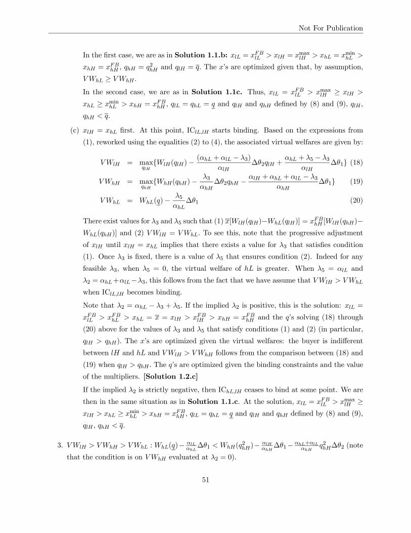
Not For Publication

In the first case, we are as in Solution 1.1.b: xlL = xFBlL > xlH = xmaxlH > xhL = xminhL >

xhH = xFBhH , qhH = q2hH and qlH = q. The x’s are optimized given that, by assumption,

VWhL ≥ VWhH .

In the second case, we are as in Solution 1.1c. Thus, xlL = xFBlL > xmaxlH ≥ xlH >

xhL ≥ xminhL > xhH = xFBhH , qlL = qhL = q and qlH and qhH defined by (8) and (9), qlH ,

qhH < q.

(c) xlH = xhL first. At this point, IClL,lH starts binding. Based on the expressions from

(1), reworked using the equalities (2) to (4), the associated virtual welfares are given by:

VWlH = maxqlH

{WlH(qlH)−(αhL + αlL − λ3)

αlH∆θ2qlH +

αhL + λ5 − λ3αlH

∆θ1} (18)

VWhH = maxqhH

{WhH(qhH)−λ3αhH

∆θ2qhH −αlH + αhL + αlL − λ3

αhH∆θ1} (19)

VWhL = WhL(q)−λ5αhL∆θ1 (20)

There exist values for λ3 and λ5 such that (1) x[WlH(qlH)−WhL(qlH)] = xFBhH [WlH(qhH)−WhL(qhH)] and (2) VWlH = VWhL. To see this, note that the progressive adjustment

of xlH until xlH = xhL implies that there exists a value for λ3 that satisfies condition

(1). Once λ3 is fixed, there is a value of λ5 that ensures condition (2). Indeed for any

feasible λ3, when λ5 = 0, the virtual welfare of hL is greater. When λ5 = αlL and

λ2 = αhL+αlL−λ3, this follows from the fact that we have assume that VWlH > VWhL

when IClL,lH becomes binding.

Note that λ2 = αhL − λ3 + λ5. If the implied λ2 is positive, this is the solution: xlL =

xFBlL > xFBhL > xhL = x = xlH > xFBlH > xhH = xFBhH and the q’s solving (18) through

(20) above for the values of λ3 and λ5 that satisfy conditions (1) and (2) (in particular,

qlH > qhH). The x’s are optimized given the virtual welfares: the buyer is indifferent

between lH and hL and VWlH > VWhH follows from the comparison between (18) and

(19) when qlH > qhH . The q’s are optimized given the binding constraints and the value

of the multipliers. [Solution 1.2.c]

If the implied λ2 is strictly negative, then IChL,lH ceases to bind at some point. We are

then in the same situation as in Solution 1.1.c. At the solution, xlL = xFBlL > xmaxlH ≥xlH > xhL ≥ xminhL > xhH = xFBhH , qlL = qhL = q and qlH and qhH defined by (8) and (9),

qlH , qhH < q.

3. VWlH > VWhH > VWhL :WhL(q)− αlLαhL∆θ1 < WhH(q

2hH)−

αlHαhH∆θ1− αhL+αlL

αhHq2hH∆θ2 (note

that the condition is on VWhH evaluated at λ2 = 0).

51

Not For Publication

In this case, we ideally want to decrease xhL, first to the benefit of xlH (then, possibly to

the benefit of xhH). Doing this while keeping xFBhH [WlH(qhH)−WhL(qhH)] = xlH [WlH(qlH)−WhL(qlH)], requires that we decrease λ2 (cf. (16) and (17)). This decreases VWlH and in-

creases VWhH , but given the condition on this case, the ordering of virtual welfares is not

affected. Thus, this process continues until, either we reach λ2 = 0 (and thus IChL,lH ceases

to bind) or xlH = xhL (and thus IClL,lH starts binding).

(a) We reach xlH = xhL when λ2 > 0 : This implies that IClL,lH becomes binding in the

process. Optimizing from now on with constraints IClH,hH , IClL,lH , IClL,hL, IChL,lH

and IChL,hH binding requires that we keep xlH = xhL. The virtual welfares are given

by (18), (19) and (20). Like in part 1, scenario 2, case 2c, we proceed by first looking

for values of λ3, λ5 and q’s such that (1) x[WlH(qlH) −WhL(qlH)] = xFBhH [WlH(qhH) −WhL(qhH)], i.e. UlL,hL = UlL,lH and UhL,hH = UhL,hH and (2) VWlH = VWhL.

If the implied λ2 is positive, then this is the solution (solution 1.2.c) because condition

(1) implies that qlH > qhH , which in turn ensures that VWlH = VWhL > VWhH . The

x’s are optimized, and so are the q’s.

If the implied λ2 is negative, then we are as in part I, scenario 1, case 3: the binding

constraints are IClL,lH , IClL,hL, IClH,hH and IChL,hH . This leads to solutions 1.1.c, 1.1.d

or 1.1.e.

(b) We reach λ2 = 0 when xlH ≤ xhL. We can continue to increase xlH at the expense

of xhL, and afterwards if necessary increase xhH at the expense of xhL until IClL,lH

starts binding. (IChL,lH no longer binds because increasing xlH beyond xhL means that

xhH [WlH(qhH) −WhL(qhH)] < xlH [WlH(qlH) −WhL(qlH)]). The case then reduces to

part 1, scenario 1, case 3, implying one of solutions 1.1.c, 1.1.d or 1.1.e apply.

Proof of part II of Theorem 1: WlH (q)−WhL (q) < 0 i.e. ∆θ1 < q∆θ2

The binding constraints in the buyer-optimal efficient mechanism are IClH,hH , IChL,lH and IClL,hL.

The buyer’s resulting expected utility is given by

αlHxlH [WlH(qlH) +αhL + αlL

αlH∆θ1 −

αhL + αlLαlH

qlH∆θ2] + αhHxhH [WhH(qhH)−αlH + αhL + αlL

αhH∆θ1]

+αhLxhL[WhL(qhL)−αlLαhL∆θ1] + αlLxlLWlL(qlL) (21)

Keeping the probabilities fixed at xk = xFBk , optimizing the q’s requires that qlH be set equal to

q2lH = argmax{WlH(qlH) +αhL + αlL

αlH∆θ1 −

αhL + αlLαlH

qlH∆θ2} (22)

52

Not For Publication

This reduces the informational rents of hL and lL. By Lemma 7(1), we know that UlL,hL > UlL,lH

as long as UhL,lH ≥ UhL,hH . Hence, we need to consider only two scenarios, depending on whether

IChL,hH binds at q2LH :

Scenario 1: At q2lH , UhL,lH ≥ UhL,hH , i.e., xFBlH [WlH(q2lH)−WhL(q

2lH)] ≤ xFBhH [WlH(q)−WhL(q)]

In this case, all IC constraints remain satisfied as we decrease qlH to q2lH . Note that WlH(q2lH) −

WhL(q2lH) ≡ ∆θ1 −∆θ2q2lH < 0. We now consider the optimization of the probabilities of winning.

From (21), the virtual welfare associated with lL is the largest. This leaves four cases depending

on the relative ranking of lH, hH and hL:

1. VWhL ≥ VWlH ≥ VWhH : [WhL(q)− αlLαhL∆θ1] ≥ [WlH(q

2lH)+

αhL+αlLαlH

∆θ1−αhL+αlLαlH

q2lH∆θ2] ≥[WhH(q)− αlH+αhL+αlL

αhH∆θ1] [Solution 2.1.a]

The optimal probabilities of winning are xk = xFBk since the ranking of the virtual welfares

corresponds to the ranking of the first best welfares. All IC constraints are satisfied. The x’s

and q’s are optimized given the binding constraints.

2. VWlH > VWhH ≥ VWhL : [WlH(q2lH)+

αhL+αlLαlH

∆θ1−αhL+αlLαlH

q2lH∆θ2] > WhH(q)−αlH+αhL+αlLαhH

∆θ1 ≥[WhL(q)− αlL

αhL∆θ1] ; or

VWlH > VWhL ≥ VWhH : [WlH(q2lH)+

αhL+αlLαlH

∆θ1−αhL+αlLαlH

q2lH∆θ2] > [WhL(q)− αlLαhL∆θ1] ≥

WhH(qhH)− αlH+αhL+αlLαhH

∆θ1

The buyer would like to increase xlH at the expense of xhL. Doing this does not affect the

supplier hL’s IC constraint: UhL,lH ≥ UhL,hH corresponds to xlH [WlH(q2lH) −WhL(q

2lH)] ≤

xFBhH [WlH(q) −WhL(q)] and WlH(q2lH)−WhL(q

2lH) < 0. Moreover, as long as xhL > xlH , the

change in xlH does not affect lL’s IC constraint either (Lemma 7(1)). Thus, changing xlH

does not initially affect the virtual welfares.

When we reach xlH = xhL = x, IClL,lH starts binding since UlL,hL = xhL∆θ1 − xlH∆θ1 +

xlHq2lH∆θ2 + xhH∆θ1 and UlL,lH = xlHq

2lH∆θ2 + xhH∆θ1. Define λ∗5 ∈ (0, αlL), the value of

λ5 that equalizes the virtual welfares associated with lH and hL:

WlH(q2lH) +

(αhL + λ∗5)

αlH∆θ1 −

αhL + αlLαlH

∆θ2q2lH =WhL(q)−

λ∗5αhL∆θ1 (23)

(from (1) to (4)). Such a value for λ5 exists. When λ5 = 0, the virtual welfare associated with

hL is larger. When λ5 = αlL, the virtual welfare of lH is bigger by assumption. Note that

this process does not affect the virtual welfare associated with hH, which remains unchanged.

(a) [Solution 2.1.b] If at λ∗5, V WlH = VWhL > VWhH , then the solution is qlH = q2lH ,

qhH = q and qhL = qlL = q and xlL = xFBlL , xhH = xFBhH , and xlH = xhL = x. All IC

53

Not For Publication

constraints are satisfied. The q’s and the x’s are optimized given the binding constraints

(in particular, the buyer is indifferent between lH and hL, but strictly prefer these to

hH).

(b) If at λ∗5, V WlH = VWhL < VWhH , the buyer prefers hH to lH or hL. He increases his

expected utility by raising xhH while keeping UlL,lH = UlL,hL, that is, xlH = xhL, and

λ5 = λ∗5. This process does not initially affect any of the virtual welfares until IChL,hH

starts binding (this happens at xhL = xlH > xhH given that qlH = q2lH < qhH = q when

UhL,hH ≤ UhL,lH).

From then on, IClH,hH , IClL,lH , IClL,hL, IChL,lH and IChL,hH are all binding. The ex-

pressions for the resulting virtual welfares are given by:

VWlH = maxqlH

{WlH(qlH)−(αhL + αlL − λ3)

αlH∆θ2qlH +

αhL + λ5 − λ3αlH

∆θ1} (24)

VWhH = maxqhH

{WhH(qhH)−λ3αhH

∆θ2qhH −αlH + αhL + αlL − λ3

αhH∆θ1} (25)

VWhL = WhL(q)−λ5αhL∆θ1 (26)

The buyer increases his expected utility by continuing to increase xhH at the cost of xhL

and xlH , while satisfying: (1) UlL,lH = UlL,hL (thus xlH = xhL), (2) UhL,hH = UhL,lH ,

that is xlH [WlH(qlH)−WhL(qlH)] = xhH [WlH(qhH)−WhL(qhH)], and (3) VWlH = VWhL.

This requires an increase in λ3 and a decrease in λ5, i.e. a rise in qlH and a decrease in

qhH (nonetheless, q2lH < qlH < qhH remains as long as VWlH ≤ VWhH as is apparent

from (24) and (25)).3

This process stops when either VWhH = VWlH = VWhL or we hit a non negativity

constraint for the multiplier λ2 = αhL + λ5 − λ3.

i. [Solution 2.1.d] Suppose VWhH = VWlH = VWhL at a point where λ2 ≥ 0.

Then we have reached the solution. The q’s are defined from (24) and (25) for

the values of λ3 and λ5 that equalize the virtual welfares (note that this implies

that qlH < qhH , so that, in turn, UhL,hH = UhL,lH implies xlH > xhH as required

for incentive compatibility). The x’s are such that xlL = xFBlL , and xFBlH > xlH =

xhL > xhH > xFBhH with N(αlLxFBlL + αlHxlH + αhLxhL + αhHxhH) = 1.4 All IC

constraints are satisfied. The q’s are optimized given the binding constraints. The

3Formally, we have four equations (the three constraints mentioned in the text, plus the feasibility constraint

N(αlLxFBlL +αlHxlH +αhLxhL +αhHxhH) = 1) and five unknowns: xhH , xhL, xlH and λ3 and λ5 (the q’s are

determined on the basis of the λ’s by (24) and (25)). Thus any value for xhH pins down the other variables.4No other feasibility constraint for the probabilities of winning binds, except for the one-type constraint for xlL.

54

Not For Publication

x’s are optimized given the resulting virtual welfares (the buyer is indifferent among

lH, hL and hH).

ii. [Solution 2.1.e] Suppose λ2 reaches zero at a point where VWhH > VWlH =

VWhL.

Let λ∗∗5 , the value of λ5 at this point. We also have q2lH < qlH < qhH and xlH =

xhL > xhH at this point. The buyer further increases his utility by increasing xhH

at the cost of xlH and xhL, while keeping UlL,lH = UlL,hL and VWlH = VWhL (i.e.

λ5 = λ∗∗5 and the q’s are fixed at qlH < qhH).5 This process at first does not affect

the virtual welfares (since λ5 is fixed, we keep having VWhH > VWlH = VWhL),

until IClL,hH starts binding.6 At this stage we have:

UlL,lH = xhH∆θ1 + xlHqlH∆θ2 = UlL,hH = xhH∆θ1 + xhHqhH∆θ2

= UlL,hL = xhL∆θ1 + xhHqhH∆θ2

thus xhL = xhH < xlH . To keep increasing the buyer’s welfare while satisfying all

three constraints out of lL requires that we keep xhL = xhH . Thus we increase

both xhL and xhH at the expense of xlH (this will indeed increase the buyer’s

utility since VWhH > VWlH = VWhL), and adjust the q’s as needed, that is, we

increase qlH and decrease qhH . We do this until VWlH = VWhL = VWhH . We

have then reached the solution. At the solution, qlH < qhH and xlL = xFBlL , and

xFBlH > xlH > xhL = xhH > xFBhH with N(αlLxFBlL +αlHxlH+αhLxhL+αhHxhH) = 1.

3. VWhL > VWhH > VWlH : [WhL(q)− αlLαhL∆θ1] > [WhH(q)− αlH+αhL+αlL

αhH∆θ1] > [WlH(q

2lH)+

αhL+αlLαlH

∆θ1 − αhL+αlLαlH

q2lH∆θ2] ; or

VWhH > VWhL > VWlH : WhH(q)− αlH+αhL+αlLαhH

∆θ1 > [WhL(q)− αlLαhL∆θ1] > [WlH(q

2lH) +

αhL+αlLαlH

∆θ1 − αhL+αlLαlH

q2lH∆θ2]

In this case, the buyer would like to increase xhH at the expense of xlH . As we increase xhH

and decrease xlH , we reach a point where xlH [WlH(q2lH)−WhL(q

2lH)] = xhH [WlH(q)−WhL(q)],

that is, IChL,hH starts binding.

A candidate solution is defined by the value of λ2 ∈ (0, αhL + αlL) that equates VWlH and

5The exact way in which xlH and xhL are decreased is determined by UlL,lH = UlL,hL, i.e. xlHqlH∆θ2+xhH∆θ1 =

xhL∆θ1 + xhHqhH∆θ2 and the feasibility constraint N(αlLxFBlL + αlHxlH + αhLxhL + αhHxhH) = 1.6This is the only constraint that can bind in the process. No new constraint can bind out of lH since UlH = xhH∆θ1

increases and alternatives decrease. No new constraint can bind out of hL because ∆θ1 −∆θ2qhH < 0 given that

qhH > qlH > q2lH and VWhH ≥ VWlH .

55

Not For Publication

VWhH :

maxqlH

{WlH(qlH)+λ∗2αlH∆θ1−

λ∗2αlH∆θ2qlH} = max

qhH{WhH(qhH)−

αlH + λ∗2αhH

∆θ1−αhL + αlL − λ∗2

αhH∆θ2qhH}

(27)

(from (1) to (4)). Such value for λ2 exists since the virtual welfare of lH is larger than that

of hH at λ2 = 0, and smaller at λ2 = αhL + αlL by assumption. By inspection of (27), this

happens at αhL+αlL−λ∗2αhH

<λ∗2αlH

that is, the resulting q’s are such that q2lH < qlH < qhH . Finally,

we require that UhL,lH = UhL,hH , that is, xlH [WlH(qlH) − WhL(qlH)] = xhH [WlH(qhH) −WhL(qhH)] which implies that xlH > xhH as required by incentive compatibility.

This process only affected VWhL and VWhH . If VWhL > VWhH = VWlH at this point, then

this is indeed the solution. The other variables are set such that xlL = xFBlL , xhL = xFBhL ,

and qhL = qlL = q. The q’s are optimized given the values of the multipliers and the binding

constraints. The x’s are optimized given the resulting virtual welfares. All IC constraints are

satisfied (IClL,lH satisfied given Lemma 7(1)). [Solution 2.1.c]

If VWhL < VWhH = VWlH , the buyer can further increase his expected utility by increasing

xhH and xlH at the cost of xhL. He does so while keeping λ2 = λ∗2 so that VWhH = VWlH . The

exact way in which xhH and xlH are increased is pinned down by xlH [WlH(qlH)−WhL(qlH)] =

xhH [WlH(qhH)−WhL(qhH)]. This process does not affect the virtual welfare, until xhL = xlH

at which point IClL,lH starts binding. We are now in a situation where IClH,hH , IClL,lH ,

IClL,hL, IChL,lH and IChL,hH are all binding and VWhL < VWhH = VWlH . From then on,

the virtual welfares are those defined in (24) - (26). Let λ∗5 such that VWlH = VWhL.

Since there is no change in λ3, the q’s are not affected (qlH < qhH) and the x’s implicitly

defined by xlH = xhL and UhL,hH = UhL,lH are not affected either. Thus we are exactly

in the same situation as in 2(b) above, and the proof thus proceeds along the same lines:

we look for a solution where IClH,hH , IClL,lH , IClL,hL, IChL,lH and IChL,hH are binding and

VWhL = VWhH = VWlH , or IClH,hH , IClL,lH , IClL,hL, IClL,hH and IChL,hH are binding and

VWhL = VWhH = VWlH . [Solution 2.1.d or 2.1.e]

4. VWhH > VWlH > VWhL : WhH(q) − αlH+αhL+αlLαhH

∆θ1 > [WlH(q2lH) +

αhL+αlLαlH

∆θ1 −αhL+αlL

αlHq2lH∆θ2] > [WhL(q)− αlL

αhL∆θ1]

Given the ordering of virtual welfares, the buyer is first tempted to increase xhH at the

expense of xhL.7 Two things can happen in the process: (1) IClL,lH starts binding (this

happens at xFBlH = xhL because UlL,lH = xlH∆θ2q2lH + xhH∆θ1 and UlL,hL = xhL∆θ1 −

xlH∆θ1 + xlH∆θ2q2lH + xhH∆θ1), (2) IChL,hH starts binding (this happens at a point where

7That is, keeping the equality N(αlLxFBlL + αlHxFBlH + αhLxhL + αhHxhH) = 1.

56

Not For Publication

xhH < xFBlH since xhH [WlH(q) −WhL(q)] = xFBlH [WlH(q2lH) −WhL(q

2lH)] at that point, and

WlH(q2lH)−WhL(q

2lH) < 0 from the definition of scenario 1). We examine each case in turn.

(a) IClL,lH binds first (xFBlH = xhL)

Let λ∗5, the value of λ5 that equalizes VWlH and VWhL. This was defined in (23). We now

have VWhH > VWlH = VWhL. Thus the buyer can increase his welfare by increasing

xhH . The rest of the solution is as described in 2(b) above. [Solution 2.1.d or Solution

2.1.e].

(b) IChL,hH binds first:

This happens at xhL > xFBlH > xhH (the first inequality comes from the fact that

IChL,hH binds first; the second inequality comes from the fact that qlH < qhH = q at

the point where IChL,hH starts binding). Increasing further xhH at the expense of xhL,

while keeping xFBlH [WlH(qlH) −WhL(qlH)] = xhH [WlH(qhH) −WhL(qhH)] requires that

we decrease qhH and increase qlH . This corresponds to a rise in λ3, a decrease in VWhH

and an increase in VWlH . This process stops when either VWlH = VWhH or xlH = xhL

whichever comes first (note at this stage xlH = xhL > xhH and IClL,lH starts binding).

If VWlH = VWhH first, we can continue to increase the buyer’s utility by decreasing

xhL, this time to the benefit of both lH and hH while keeping VWlH = VWhH and

UhL,hH = UhL,lH (note that this implies qlH < qhH and xhL > xhH). This process

continues until xhL = xlH at which point IClL,lH starts binding.

Thus, in both events, we reach a point where IClH,hH , IClL,lH , IClL,hL, IChL,lH and

IChL,hH are all binding. From then on, the virtual welfares are those defined in (24) -

(26). Let λ∗5 such that VWlH = VWhL. Since there is no change in λ3, the q’s are not

affected (qlH < qhH) and the x’s implicitly defined by xlH = xhL and UhL,hH = UhL,lH

are not affected either. Thus we are exactly in the same situation as in 2(b) above,

and the proof thus proceeds along the same lines: we look for a solution where IClH,hH ,

IClL,lH , IClL,hL, IChL,lH and IChL,hH are binding and VWhL = VWhH = VWlH , or

IClH,hH , IClL,lH , IClL,hL, IClL,hH and IChL,hH are binding and VWhL = VWhH =

VWlH . [Solution 2.1.d or 2.1.e]

Scenario 2: At q2lH , UhL,hH > UhL,lH that is, xFBlH [WlH(q2lH)−WhL(q

2lH)] > xFBhH [WlH(q)−WhL(q)]

In this case, IChL,hH becomes binding as we decrease qlH towards q2lH . To decrease the rents of

hL and lL, we now need to decrease qlH and qhH , holding UhL,hH = UhL,lH . The optimal q’s are

57

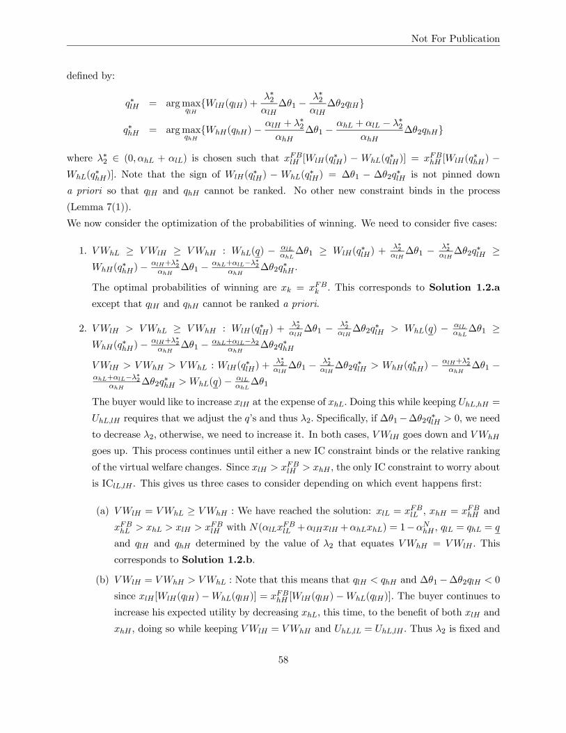
Not For Publication

defined by:

q∗lH = argmaxqlH

{WlH(qlH) +λ∗2αlH∆θ1 −

λ∗2αlH∆θ2qlH}

q∗hH = argmaxqhH

{WhH(qhH)−αlH + λ∗2αhH

∆θ1 −αhL + αlL − λ∗2

αhH∆θ2qhH}

where λ∗2 ∈ (0, αhL + αlL) is chosen such that xFBlH [WlH(q∗lH) − WhL(q

∗lH)] = xFBhH [WlH(q

∗hH) −

WhL(q∗hH)]. Note that the sign of WlH(q

∗lH) − WhL(q

∗lH) = ∆θ1 − ∆θ2q∗lH is not pinned down

a priori so that qlH and qhH cannot be ranked. No other new constraint binds in the process

(Lemma 7(1)).

We now consider the optimization of the probabilities of winning. We need to consider five cases:

1. VWhL ≥ VWlH ≥ VWhH : WhL(q) − αlLαhL∆θ1 ≥ WlH(q

∗lH) +

λ∗2αlH∆θ1 − λ∗2

αlH∆θ2q

∗lH ≥

WhH(q∗hH)−

αlH+λ∗2

αhH∆θ1 − αhL+αlL−λ∗2

αhH∆θ2q

∗hH .

The optimal probabilities of winning are xk = xFBk . This corresponds to Solution 1.2.a

except that qlH and qhH cannot be ranked a priori.

2. VWlH > VWhL ≥ VWhH : WlH(q∗lH) +

λ∗2αlH∆θ1 − λ∗2

αlH∆θ2q

∗lH > WhL(q) − αlL

αhL∆θ1 ≥

WhH(q∗hH)−

αlH+λ∗2

αhH∆θ1 − αhL+αlL−λ2

αhH∆θ2q

∗hH

VWlH > VWhH > VWhL : WlH(q∗lH) +

λ∗2αlH∆θ1 − λ∗2

αlH∆θ2q

∗lH > WhH(q

∗hH) −

αlH+λ∗2

αhH∆θ1 −

αhL+αlL−λ∗2αhH

∆θ2q∗hH > WhL(q)− αlL

αhL∆θ1

The buyer would like to increase xlH at the expense of xhL. Doing this while keeping UhL,hH =

UhL,lH requires that we adjust the q’s and thus λ2. Specifically, if ∆θ1−∆θ2q∗lH > 0, we need

to decrease λ2, otherwise, we need to increase it. In both cases, VWlH goes down and VWhH

goes up. This process continues until either a new IC constraint binds or the relative ranking

of the virtual welfare changes. Since xlH > xFBlH > xhH , the only IC constraint to worry about

is IClL,lH . This gives us three cases to consider depending on which event happens first:

(a) VWlH = VWhL ≥ VWhH : We have reached the solution: xlL = xFBlL , xhH = xFBhH and

xFBhL > xhL > xlH > xFBlH with N(αlLxFBlL +αlHxlH +αhLxhL) = 1−αNhH , qlL = qhL = q

and qlH and qhH determined by the value of λ2 that equates VWhH = VWlH . This

corresponds to Solution 1.2.b.

(b) VWlH = VWhH > VWhL : Note that this means that qlH < qhH and ∆θ1−∆θ2qlH < 0

since xlH [WlH(qlH)−WhL(qlH)] = xFBhH [WlH(qlH)−WhL(qlH)]. The buyer continues to

increase his expected utility by decreasing xhL, this time, to the benefit of both xlH and

xhH , doing so while keeping VWlH = VWhH and UhL,lL = UhL,lH . Thus λ2 is fixed and

58

Not For Publication

so are qlH and qhH . Therefore xlH > xhH . This process continues until xhL = xlH at

which point IClL,lH starts binding. From then on, the virtual welfares are those defined

in (24) - (26). (note that λ2 = αhL + λ5 − λ3). Let λ∗5 such that VWlH = VWhL. Since

there is no change in λ3, the q’s are not affected (qlH < qhH) and the x’s implicitly

defined by xlH = xhL and UhL,hH = UhL,lH are not affected either. Thus we are exactly

in the same situation as in scenario 1, 2(b) above (VWhH > VWlH = VWhL), and the

proof thus proceeds along the same lines. [Solution 2.1.d or 2.1.e]

(c) xhL = xlH , i.e. IClL,lH starts binding. From then on, IClH,hH , IClL,lH , IClL,hL, IChL,lH

and IChL,hH are all binding. The virtual welfares are those defined in (24) - (26). (note

that λ2 = αhL+λ5−λ3). Let λ∗5 such that VWlH = VWhL. Since there is no change in λ3,

the q’s are not affected and the x’s implicitly defined by xlH = xhL and UhL,hH = UhL,lH

are not affected either. If VWlH = VWhL > VWhH , we have reached the solution:

xlL = xFBlL , xFBhL > xlH = xhL = x > xFBlH , xhH = xFBhH , qlH , qhH < q and qlL = qhL = q.

All IC constraints are satisfied and the q’s and x’s are optimal given the resulting virtual

welfares. [Solution 1.2.c]

If VWlH = VWhL < VWhH , we can conclude that qlH < qhH and ∆θ1 − ∆θ2qlH < 0

since xlH [WlH(qlH)−WhL(qlH)] = xFBhH [WlH(qlH)−WhL(qlH)].We are thus in the same

situation as in scenario 1, 2(b) above. [Solution 2.1.d or 2.1.e]

3. VWhL > VWhH > VWlH :WhL(q)− αlLαhL∆θ1 > WhH(q

∗hH)−

αlH+λ∗2

αhH∆θ1−αhL+αlL−λ∗2

αhH∆θ2q

∗hH >

WlH(q∗lH) +

λ∗2αlH∆θ1 − λ∗2

αlH∆θ2q

∗lH .

(Note that this implies q∗lH < q∗hH and∆θ1−∆θ2q∗lH < 0 given that xFBlH [WlH(q∗lH)−WhL(q

∗lH)]

= xFBhH [WlH(q∗hH)−WhL(q

∗hH)]). The buyer wants to increase xhH at the expense of xlH . This

requires adjusting λ2 to maintain the equality xlH [WlH(qlH)−WhL(qlH)] = xhH [WlH(qhH)−WhL(qhH)]. Specifically, λ2 decreases, qlH increases and qhH decreases, until VWhH = VWlH .

This occurs at xlH > xhH . Indeed, at xlH = xhH , qlH = qhH thus αhL+αlL−λ2αhH

∆θ2qhH =λ2αlH∆θ2qlH implying that VWhH < VWlH . The solution is thus xlL = xFBlL , xhL = xFBhL and

xFBlH > xlH > xhH > xFBhH and qlH < qlH < qhH < q. This corresponds to solution 2.1.c

4. VWhH ≥ VWlH ≥ VWhL : WhH(q∗hH) −

αlH+λ∗2

αhH∆θ1 − αhL+αlL−λ∗2

αhH∆θ2q

∗hH ≥ WlH(q

∗lH) +

λ∗2αlH∆θ1 − λ∗2

αlH∆θ2q

∗lH ≥WhL(q)− αlL

αhL∆θ1

Note that this implies that q∗lH < q∗hH and ∆θ1 −∆θ2q∗lH < 0. Define λ∗∗2 ∈ (0, λ∗2) such that

maxqhH

{WhH(qhH)−αlH + λ∗∗2

αhH∆θ1−

αhL + αlL − λ∗∗2αhH

∆θ2qhH} = maxqlH

{WlH(qlH)+λ∗∗2αlH∆θ1−

λ∗∗2αlH∆θ2qlH}

(28)

59

Not For Publication

This implies q∗lH < qlH < qhH < q∗hH and VWlH = VWhH > VWhL.

>From there, the buyer can increase his expected utility by increasing xhH and xlH at the cost

of xhL. He does so while keeping λ2 = λ∗∗2 so that VWhH = VWlH . The exact way in which

xhH and xlH are increased is pinned down by xlH [WlH(qlH)−WhL(qlH)] = xhH [WlH(qhH)−WhL(qhH)]. This process does not affect the virtual welfare, until xhL = xlH at which point

IClL,lH starts binding. We are now in a situation where IClH,hH , IClL,lH , IClL,hL, IChL,lH and

IChL,hH are all binding and VWhL < VWhH = VWlH . From then on, the virtual welfares are

those defined in (24) - (26) (note that λ2 = αhL+λ5−λ3). Let λ∗5 such that VWlH = VWhL.

Since there is no change in λ3, the q’s are not affected (qlH < qhH) and the x’s implicitly

defined by xlH = xhL and UhL,hH = UhL,lH are not affected either. Thus we are exactly in

the same situation as in 2(b) above. [Solution 2.1.d or 2.1.e]

5. VWhH > VWhL > VWlH : WhH(q∗hH) −

αlH+λ∗2

αhH∆θ1 − αhL+αlL−λ∗2

αhH∆θ2q

∗hH > WhL(q) −

αlLαhL∆θ1 > WlH(q

∗lH) +

λ∗2αlH∆θ1 − λ∗2

αlH∆θ2q

∗lH

We are again in a situation where q∗lH < q∗hH and ∆θ1 −∆θ2q∗hH < 0. The buyer would like

to increase xhH at the expense of xlH . Doing so while keeping xlH [WlH(qlH)−WhL(qlH)] =

xhH [WlH(qhH) −WhL(qhH)] requires an adjustment in λ2, leading to VWlH decreasing and

VWhH increasing. This process continues until we reach λ∗∗2 which corresponds to VWlH =

VWhH (as defined in (28)). Since ∆θ1−∆θ2q∗hH < 0, the corresponding qualities and x’s are

such that q∗lH < qlH < qhH < q∗hH and xhH < xlH .

We now need to distinguish two cases depending whether VWhL > VWlH = VWhH or

VWlH = VWhH > VWhL.

(a) VWhL > VWlH = VWhH : Then we have reached the solution: xlL = xFBlL , xhL = xFBhL

and xFBlH > xlH > xhH > xFBhH , qlL = qhL = q and q∗lH < qlH < qhH < q∗hH as defined by

(28). This corresponds to Solution 2.1.c.

(b) VWlH = VWhH > VWhL : the buyer further increases his expected utility by increases

xlH and xhH at the expense of xhL while keeping VWhH = VWlH (that is keeping

λ2 and the q’s fixed) and UhL,lH = UhL,hH (thus xhH < xlH). This process does not

affect the virtual welfares until xhL = xlH and IClL,lH starts binding. We are now in

a situation where IClH,hH , IClL,lH , IClL,hL, IChL,lH and IChL,hH are all binding and

VWhL < VWhH = VWlH . From then on, the virtual welfares are those defined in (24)

- (26) (note that λ2 = αhL + λ5 − λ3). Let λ∗5 such that VWlH = VWhL. Since there is

no change in λ3, the q’s are not affected (qlH < qhH) and the x’s implicitly defined by

xlH = xhL and UhL,hH = UhL,lH are not affected either. Thus we are exactly in the same

60

Not For Publication

situation as in 2(b) above, and the proof thus proceeds along the same lines. [Solution

2.1.d or 2.1.e]

61