Embed Size (px)
Citation preview

ICON 2020
17th International Conference on Natural LanguageProcessing
Proceedings of the Workshop
December 18 - 21, 2020Indian Institute of Technology Patna, India

©2020 NLP Association of India (NLPAI)
ii

Introduction
Welcome to the ICON 2020 Workshop on Joint NLP Modelling for Conversational AI.
Virtual Assistants/Dialog Systems are spanning from cloud-based systems to embedded devicesformulating a hybrid architecture for several reasons such as privacy of the data, faster processing, offlineinteraction, personalization etc. There are several NLP tasks running as part of the Virtual Assistantexample Domain Classification, Intent Determination, Slot Extraction, Dialog Management, NaturalLanguage Generation, Text to Speech and Automatic Speech Recognition. Thus, in both cloud andembedded devices, it is necessary to combine various NLP tasks to improve latency and memory usage.Additionally, a joint NLP model is suitable for both cloud and embedded devices processing.
Virtual Assistants/Dialog Systems are also capable of learning by themselves from various informationaccessible to it. For example, contextual data, personal data, queries, unhandled or failed queries etc. Itis a very interesting area to explore how a joint model can incrementally learn from the data available tothe Virtual Assistant.
The goal of this workshop is to bring together NLP researchers and practitioners in different fields,alongside experts in speech and machine learning, to discuss the current state-of-the-art and newapproaches, to share insights and challenges, to bridge the gap between academic research and real-worldproduct deployment, and to shed the light on future directions. “Joint NLP modelling for ConversationalAI” will be a one-day workshop including keynotes, spotlight talks, posters, and panel sessions. Inkeynote talks, senior technical leaders from industry and academia will share insights on the latestdevelopments of the field. An open call for papers will be announced to encourage researchers andstudents to share their prospects and latest discoveries. The panel discussion will focus on the challenges,future directions of conversational AI research, bridging the gap in research and industrial practice, aswell as audience suggested topics.
We received 16 submissions, and after a rigorous review process, we only accepted 6 papers. The overallacceptance rate for the workshop was 37.5%.
Joint NLP modelling for Conversational AI ICON 2020 OrganizersRanjan Kumar Samal, Bixby AI, Samsung ElectronicsPraveen Kumar GS, Bixby AI, Samsung ElectronicsSiddhartha Mukherjee, Bixby AI, Samsung Electronics
iii


Organizers
Ranjan Kumar Samal - Architect of NLU, Samsung Research Institute-BangalorePraveen Kumar GS - Director of NLU, Samsung Research Institute-BangaloreSiddhartha Mukherjee - Engg. Leader of NLU, Samsung Research Institute-Bangalore
Program Committee:
• Members from Samsung R&D Institute Bangalore
– Gaurav Mathur– Anish Nediyachanth– Bharatram Natarajan– Dr. Priyadarshini Pai– Dr. Sandip Bapat– Dr. Jayesh Mundayadan Koroth– Dr. Nitya Tiwari– Dr. Hardik Bhupendra Sailor– Dr. Shekhar Nayak– Dr. Mahaboob Ali Basha Shaik
• Members from Samsung Electronics, Suwon, South Korea
– Sojeong Ha– Dr. Jun-Seong Kim
• Members from IIT-Patna
– Dr. Asif Ekbal, Professor, Department of Comp Sc & Engg, IIT Patna– Dr. Sriparna Saha, Professor, Department of Comp Sc & Engg, IIT Patna
• Members from IIT-Palakkad
– Dr. Mrinal kanti Das, Assistant Professor, CSE, IIT Palakkad
• Members from POSTECH, South Korea
– Dr. Jinwoo Park, CSE, POSTECH, Republic of Korea
v


Table of Contents
Neighbor Contextual Information Learners for Joint Intent and Slot PredictionBharatram Natarajan, Gaurav Mathur and Sameer Jain . . . . . . . . . . . . . . . . . . . . . . . . . . . . . . . . . . . . . . . 1
Unified Multi Intent Order and Slot Prediction using Selective Learning PropagationBharatram Natarajan, Priyank Chhipa, Kritika Yadav and Divya Verma Gogoi . . . . . . . . . . . . . . . . 10
EmpLite: A Lightweight Sequence Labeling Model for Emphasis Selection of Short TextsVibhav Agarwal, Sourav Ghosh, Kranti CH, Bharath Challa, Sonal Kumari, Harshavardhana . and
BARATH RAJ KANDUR RAJA . . . . . . . . . . . . . . . . . . . . . . . . . . . . . . . . . . . . . . . . . . . . . . . . . . . . . . . . . . . . . . 19
Named Entity Popularity Determination using Ensemble LearningVikram Karthikeyan, B Shrikara Varna, Amogha Hegde, Govind Satwani, Shambhavi B R, Ja-
yarekha P and Ranjan Samal . . . . . . . . . . . . . . . . . . . . . . . . . . . . . . . . . . . . . . . . . . . . . . . . . . . . . . . . . . . . . . . . . . 27
Optimized Web-Crawling of Conversational Data from Social Media and Context-Based FilteringAnnapurna P Patil, Rajarajeswari Subramanian, Gaurav Karkal, Keerthana Purushotham, Jugal
Wadhwa, K Dhanush Reddy and Meer Sawood . . . . . . . . . . . . . . . . . . . . . . . . . . . . . . . . . . . . . . . . . . . . . . . . . 33
A character representation enhanced on-device Intent ClassificationSudeep Deepak Shivnikar, Himanshu Arora and Harichandana B S S . . . . . . . . . . . . . . . . . . . . . . . . 40
vii


Workshop Program
Monday, December 21, 2020
10:00 Opening Note by Praveen Kumar G S, Director and Head of NLU, SRIB
10:15 "Transformation from NLU to Multimodal NLU" by Siddhartha Mukherjee, StaffEngineering Manager of NLU, SRIB
11:00 Neighbor Contextual Information Learners for Joint Intent and Slot PredictionBharatram Natarajan, Gaurav Mathur and Sameer Jain
11:30 Unified Multi Intent Order and Slot Prediction using Selective Learning Propa-gationBharatram Natarajan, Priyank Chhipa, Kritika Yadav and Divya Verma Gogoi
12:00 EmpLite: A Lightweight Sequence Labeling Model for Emphasis Selection ofShort TextsVibhav Agarwal, Sourav Ghosh, Kranti CH, Bharath Challa, Sonal Kumari, Har-shavardhana and BARATH RAJ KANDUR RAJA
12:30 Optimized Web-Crawling of Conversational Data from Social Media and Context-Based FilteringAnnapurna P Patil, Rajarajeswari Subramanian, Gaurav Karkal, Keerthana Pu-rushotham, Jugal Wadhwa, K Dhanush Reddy and Meer Sawood
13:00 Lunch Break
14:00 AI for real-world and AI for future; Panel Discussion by Senior Thought Lead-ers at SRIB by Praveen Kumar GS, Ratnakar Rao VR, Sreevatsa DB, Ritesh Jain,Srinivasa Rao Kudavelly
15:00 Named Entity Popularity Determination using Ensemble LearningVikram Karthikeyan, B Shrikara Varna, Amogha Hegde, Govind Satwani, Shamb-havi B R, Jayarekha P and Ranjan Samal
15:30 "Discovering Subtle Information from Texts using Bayesian Models" by Dr. Mri-nal Kanti Das, Assistant Professor, CSE, IIT Palakkad
ix

16:30 A character representation enhanced on-device Intent ClassificationSudeep Deepak Shivnikar, Himanshu Arora and Harichandana B S S
17:00 Closing Note by Ranjan Samal, Architect of NLU, SRIB
x

Proceedings of the ICON 2020 Workshop on Joint NLP Modelling for Conversational AI, pages 1–9Patna, India, December 18 - 21, 2020. ©2020 NLP Association of India (NLPAI)
Neighbor Contextual Information Learners for Joint Intent and SlotPrediction
Bharatram Natarajan∗, Gaurav Mathur∗ and Sameer Jainresearch.samsung.com
{bharatram.n, gaurav.m4, sameer.jain}@samsung.com
AbstractIntent Identification and Slot Identification aretwo important task for Natural Language Un-derstanding (NLU). Exploration in this areahave gained significance using networks likeRNN, LSTM and GRU. However, modelscontaining the above modules are sequentialin nature, which consumes lot of resourceslike memory to train the model in cloud it-self. With the advent of many voice as-sistants delivering offline solutions for manyapplications, there is a need for finding re-placement for such sequential networks. Ex-ploration in self-attention, CNN modules hasgained pace in the recent times. Here we ex-plore CNN based models like Trellis and mod-ified the architecture to make it bi-directionalwith fusion techniques. In addition, we pro-pose CNN with Self Attention network calledNeighbor Contextual Information Projector us-ing Multi Head Attention (NCIPMA) architec-ture. These architectures beat state of the art inopen source datasets like ATIS, SNIPS.
1 Introduction
Intelligent Voice Assistant like Samsung Bixby,Google Assistant, Amazon Alexa and MicrosoftCortana are increasingly becoming popular. Theseassistants cater to the user request by extract-ing the user intention from the spoken utterance.NLU express the user intention in terms of in-tent label and slot tags. There is one intent la-bel for entire utterance, which signifies uniqueaction to execute. Whereas slots are tags givento tokens in utterance, which signifies extra in-formation required to execute the unique action.Slot tags are denoted in IBO format. For exam-ple, consider the utterance “what flights are avail-able from Denver to San Francisco”. We denoteIntent label as “atis flight”. We denote Slot in-formation as “O O O O O B-fromloc.city name
∗Authors contributed equally
O B-toloc.city name I-toloc.city name”. Thereis one slot tag for every token in the utterance,where “O” represents that token is not a slotand B-fromloc.city name represents that token is“Beginning of slot fromloc.city name” and “B-toloc.city name I-toloc.city name” represents thatcorresponding tokens are Beginning and Contin-uation of slot toloc.city name respectively. Weconsider Intent Identification as Classification taskand Slot tagging as sequence labelling task wherewe predict slot for each word.
Lots of work has happened in this area. Initially,research community explored both intent and slottasks as independent task. Different techniqueswere explored for intent classification. Firdauset al. (2018) created ensemble model by combininglearnings of CNN, LSTM and GRU using multi-layer perceptron to enhance intent classification.Kim et al. (2016) proposed enriched word embed-ding for making similar words together and dis-similar words farther, which aided intent detectionbetter. Yolchuyeva et al. (2020) proposed use ofself-attention for enhancing intent classification bycapturing long-range and multi-scale dependencyin data.
Similarly for slot tagging, Kurata et al. (2016)proposed use of label dependencies along with in-put sentence for enhancing slot learnings usingLSTM. Mesnil et al. (2014) suggested use of Re-current Neural Network for slot tagging task. NgocThang Vu (2016) proposed novel CNN architec-ture for slot tagging task, which also used past andfuture words information.
These individual models approach resulted inpipelined design of NLU. Where intent model willpredict intent and they use intent output in slotmodel to predict slot. This resulted in error prop-agation i.e. error in intent output resulted in slottagging errors. In addition, the intent and slot learn-ings are not available for each other to enhance
1

each task learning.
To circumvent the above limitation, researchcommunity started exploring unified model wherethey identify both intent classification and slot tag-ging. Liu and Lane (2016) proposed attention asRNN encoder as input to Decoder for predictingslot and intent by the decoder. Tingting et al. (2019)proposed exploration of attention with Bi-LSTMfor joint intent and slot prediction. Firdaus et al.(2019) suggested usage of CNN and RNN for con-textual understanding of the utterance along withCRF for label dependency to predict intent andslot. Hardalov et al. (2020) proposed intent pool-ing attention along with word features on top ofBERT for predicting intent and slot. The aboveapproaches addresses both the task using singleunified network where both the learnings are prop-agated to single network.
Further, exploration of parallel learning net-works, using common base module, with fusingof intent and slot learnings have gained momentum.Goo et al. (2018) suggested slot gate mechanismto fuse the intent attention learning with slot atten-tion learning to predict slot along with intent. Eet al. (2019) proposed a novel iteration mechanismto fuse the meanings of intent and slot subnet forpredicting intent and slot.
Inspired by the work on parallel learning net-works, where we address the intent and slot taskslearnings by each parallel network, we are propos-ing a novel architecture, Neighbor Contextual Im-portance Projector (NCIP) for learning the wordimportance in its immediate vicinity to boost itsimportance learning in the overall utterance. Weuse parallel Multi head attention on top of NCIP toproject importance phrases for each task, to predictintent and slot. We are also exploring Trellis net-work, which learns immediate neighbors in a layerand entire utterance in multiple such layers. In ad-dition, the weights of the network is shared in bothtemporal direction as well as across layers. Hence,we are proposing a bi-directional Trellis networkwith different fusion techniques, like Linear Fusion,Concatenation, to predict intent and slot to mimicbi-directional LSTM or GRU.
We organize rest of the section as follows. Sec-tion 2 describes the Proposed Approaches. Sec-tion 3 describes the experimental setup includingdataset, metrics used followed by results. Finally,we conclude and suggest future work and exten-sions.
2 Proposed Approaches
2.1 Trellis Network Based ArchitecturesBai et al. (2018) proposed a novel architecture con-taining special Temporal Convolutional Neural Net-works (T-CNN) for language modeling (LM) task.In this model, they share weights across all layersand they inject the input to deep layers.
As Trellis network has structural and algorith-mic elements from both LSTM & CNN, it achievedstate of art in various LM tasks. Therefore, we areexploring extension of the same in intent determi-nation and slot tagging.
Original Trellis Network process the input se-quence in forward direction only. We propose bi-directional network with two parallel Trellis net-work encoders, one for forward pass and one forbackward pass, for intent determination and slottagging.
2.1.1 Utterance Pre-ProcessingWe tokenize the input utterance into words. If thenumber of words is less than seq len (seq len isobtained by taking maximum of the count of wordsfor each utterance in the dataset), we pad that ut-terance with “PAD” word. We convert words toindex using dictionary of unique training wordsto incremental index. If we do not find any wordin the dictionary, than assign the index of “unk”(specially added token into dictionary to handle un-seen words). We convert every utterance of trainingbatch into list of indices to generate training dataof shape [bs, seq len]. Where ‘bs’ is batch size.
For bidirectional Trellis network, we first reversethe training utterances than apply same preprocess-ing as on original utterances.
2.1.2 Unidirectional Trellis Network BasedArchitecture
Figure 1: Unidirectional Trellis flow for joint intent andslot prediction
2

Figure 1 shows unidirectional Trellis encoder basedarchitecture. We pass input data of shape [bs,seq len] through embedding layer to represent ev-ery word with embedding size (emb size) vector.Trellis Network is used as an encoder to representinput data in [bs, seq len, nout] dimension. Wherenout is a hyper parameter of Trellis network. Forslot prediction, output of Trellis network is passedby a linear layer to produce output of shape [bs,seq len, ntag], where ntag is number of tags.
For intent determination, we first flatten the Trel-lis output than pass to output linear layer. It pro-duces output of shape [bs, nIntent], where nIntentis number of intent labels.
2.1.3 Bidirectional Trellis Network BasedArchitecture
Figure 2: Bidirectional Trellis Flow for joint intent andslot prediction
Figure 2 shows Bi-directional Trellis network. Inthis, we used two Trellis network encoders, first toprocess the input sequence as-is and the second toprocess a reversed copy of the input sequence. BothTrellis encoders generates outputs of dimension [bs, seq len , nout] . Then we pass both the Trellisnetwork outputs through fusion layer. Fusion layerdetermines the importance of each Trellis output byselectively propagating the learnings from both theoutputs. Then we predict intent by flattening thefused output and passing through dense layer withnintent [distinct intents] as final labels. We alsopredict slot by passing through dense layer withntag [distinct tags] as output label. We explore twofusion techniques in Section 2.1.4 and 2.1.5 andTrellis network in 2.1.6.
2.1.4 Masked Flip and Concatenation
Figure 3: Masked flip and concatenation
Masked flip is implemented by Gardner et al.(2017) in AllenNLP platform. As shown in Figure3, we first flip the output of backward Trellis (itbrings representation of “pad” at beginning) thanslice every example of batch on original unpaddedlength of that example. It gives representation ofpad and actual words separately, than again con-catenate pad representation at end of word represen-tation. After masked flipping of backward Trellisoutput, concatenate it with forward Trellis output.
2.1.5 Linear Fusion
Figure 4: Linear Fusion
As shown in Figure 4, we are using a linear layerto learn joint representation of forward and back-ward Trellis outputs. For it we first concatenateboth outputs at axis 1, then transpose it to bringword representation as final axis and pass by linearlayer to bring the final axis to seq len. We thentranspose the same to get seq len in first axis.
2.1.6 Trellis Network DecodedAs we are using Trellis Network to learn a tokenrepresentation from its neighbor, let us discuss
3
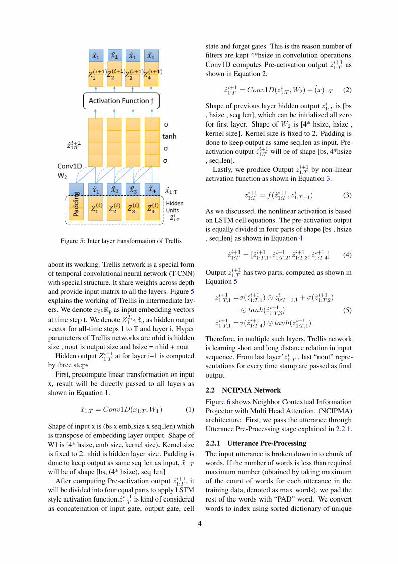
Figure 5: Inter layer transformation of Trellis
about its working. Trellis network is a special formof temporal convolutional neural network (T-CNN)with special structure. It share weights across depthand provide input matrix to all the layers. Figure 5explains the working of Trellis in intermediate lay-ers. We denote xtεRp as input embedding vectorsat time step t. We denote ZTi
1 εRq as hidden outputvector for all-time steps 1 to T and layer i. Hyperparameters of Trellis networks are nhid is hiddensize , nout is output size and hsize = nhid + nout
Hidden output Zi+11:T at for layer i+1 is computed
by three stepsFirst, precompute linear transformation on input
x, result will be directly passed to all layers asshown in Equation 1.
x1:T = Conv1D(x1:T ,W1) (1)
Shape of input x is (bs x emb size x seq len) whichis transpose of embedding layer output. Shape ofW1 is [4* hsize, emb size, kernel size). Kernel sizeis fixed to 2. nhid is hidden layer size. Padding isdone to keep output as same seq len as input, x1:Twill be of shape [bs, (4* hsize), seq len]
After computing Pre-activation output zi+11:T , it
will be divided into four equal parts to apply LSTMstyle activation function.zi+1
1:T is kind of consideredas concatenation of input gate, output gate, cell
state and forget gates. This is the reason number offilters are kept 4*hsize in convolution operations.Conv1D computes Pre-activation output zi+1
1:T asshown in Equation 2.
zi+11:T = Conv1D(zi1:T ,W2) + (x)1:T (2)
Shape of previous layer hidden output zi1:T is [bs, hsize , seq len], which can be initialized all zerofor first layer. Shape of W2 is [4* hsize, hsize ,kernel size]. Kernel size is fixed to 2. Padding isdone to keep output as same seq len as input. Pre-activation output zi+1
1:T will be of shape [bs, 4*hsize, seq len].
Lastly, we produce Output zi+11:T by non-linear
activation function as shown in Equation 3.
zi+11:T = f(zi+1
1:T , zi1:T−1) (3)
As we discussed, the nonlinear activation is basedon LSTM cell equations. The pre-activation outputis equally divided in four parts of shape [bs , hsize, seq len] as shown in Equation 4
zi+11:T = [zi+1
1:T,1, zi+11:T,2, z
i+11:T,3, z
i+11:T,4] (4)
Output zi+11:T has two parts, computed as shown in
Equation 5
zi+11:T,1 =σ(z
i+11:T,1)� zi0:T−1,1 + σ(zi+1
1:T,2)
� tanh(zi+11:T,3)
zi+11:T,1 =σ(z
i+11:T,4)� tanh(zi+1
1:T,1)
(5)
Therefore, in multiple such layers, Trellis networkis learning short and long distance relation in inputsequence. From last layer’zi1:T , last “nout” repre-sentations for every time stamp are passed as finaloutput.
2.2 NCIPMA NetworkFigure 6 shows Neighbor Contextual InformationProjector with Multi Head Attention. (NCIPMA)architecture. First, we pass the utterance throughUtterance Pre-Processing stage explained in 2.2.1.
2.2.1 Utterance Pre-ProcessingThe input utterance is broken down into chunk ofwords. If the number of words is less than requiredmaximum number (obtained by taking maximumof the count of words for each utterance in thetraining data, denoted as max words), we pad therest of the words with “PAD” word. We convertwords to index using sorted dictionary of unique
4

Figure 6: NCIPMA Architecture. Neighbor ContextualImportance Projector enhances the word importancelearning by adding the unigram, bi-gram and tri-gramword importance learnings using Multi- Head Atten-tion. Here f=1 means filter size as 1 representing un-igram, f=2 means filter size as 2 representing bi-gramand f=3 means filter size as 3 representing tri-gram.MHA means Multi-Head Attention
training words to incremental index. If we do notfind the word in the dictionary, then we assign theindex of “unkword” (specially added into sorteddictionary to handle unseen words).We map sortedwords in dictionary to index from 1 to n (number ofwords in the dictionary). We use index 0 for “PAD”word. This is the way we convert utterance to listof indices.
We pass the converted list of indices to Embed-ding layer. During training time, we have trainedEmbedding layer by masking zero index, passingweight-embedding matrix and making the matrixas trainable. We used unique training words, fromsorted dictionary, to construct weight-embeddingmatrix. We did this by taking word index from sort-ing dictionary and 300-dimension word embeddingfrom Glove Embedding for each word in uniquetraining words. Hence, Embedding layer providestrained word embedding vector for each word in-dex in the utterance during test time. This creates3-d matrix of size (1, max words, 300).
2.2.2 Neighbor Contextual InformationProjector(NCIP) Module
In this module, we pass the 3-d matrix (outputof utterance pre-processing module) through threeparallel CNN layers. Each CNN layer uses filtersize as one, two and three respectively capturingunigram, bi-gram and tri-gram word information.To learn each word information importance overother, we keep the word length same by makingpadding “same”.
We capture the importance of uni-gram, bi-gram
Figure 7: (Left) Scaled Dot-Product Attention. (Right)Multi-Head Attention consist of many scaled dot prod-uct attention in parallel.
and tri-gram word information on the uni-gramword information using Multi-Head Attention, asshown in Figure 7. Multi-Head Attention aid incapturing multiple phrases importance in the pro-vided input by passing the same input as query, keyand value and calculating the importance as shownin Figure 6. Here, we pass n-gram (uni-gram, bi-gram or tri-gram) word information as query andkey. We pass value as unigram word information.
Finally, we add the outputs of all the three Multi-Head Attention Module with unigram output.
This module aids in capturing
• Multi-phrase importance for each word.
• Multi-phrase importance for each phrasemade from two to three words as well.
Addition of the above information projects that aword is important even as a part of the phrase andnot only as a single word. We pass this informationto two parallel Multi-Head Attention Modules.
These parallel Multi-Head Attention (MHA)modules try to learn the importance of phrases foreach task in the provided input by passing the inputas Query, Key and Value as shown in Figure 7. Wepredict intent through one MHA module by firstflattening the 3 dimensional output, then by pass-ing through dense layer with distinct intent as finalhidden dimension. We predict slot through anotherMHA module, by passing through dense layer withdistinct slot as final hidden dimension.
2.3 NCIPMA With CRF
Figure 8 shows the architecture of NCIPMA withCRF. First, we pass the utterance through UtterancePre-Processing module. We pass the output of themodule to NCIP module. We use the output ofNCIP module to predict intent and slot.
5
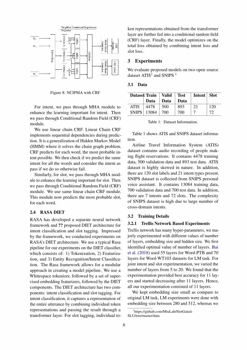
Figure 8: NCIPMA with CRF
For intent, we pass through MHA module toenhance the learning important for intent. Thenwe pass through Conditional Random Field (CRF)module.
We use linear chain CRF. Linear Chain CRFimplements sequential dependencies during predic-tion. It is a generalization of Hidden Markov Model(HMM) where it solves the chain graph problem.CRF predicts for each word, the most probable in-tent possible. We then check if we predict the sameintent for all the words and consider the intent aspass if we do so otherwise fail.
Similarly, for slot, we pass through MHA mod-ule to enhance the learning important for slot. Thenwe pass through Conditional Random Field (CRF)module. We use same linear chain CRF module.This module now predicts the most probable slot,for each word.
2.4 RASA DIETRASA has developed a separate neural networkframework and ?? proposed DIET architecture forintent classification and slot tagging. Impressedby the framework, we conducted experiments onRASA’s DIET architecture. We use a typical Rasapipeline for our experiments on the DIET classifier,which consists of: 1) Tokenization, 2) Featuriza-tion, and 3) Entity Recognition/Intent Classifica-tion. The Rasa framework allows for a modularapproach in creating a model pipeline. We use aWhitespace tokenizer, followed by a set of super-vised embedding featurizers, followed by the DIETcomponents. The DIET architecture has two com-ponents: intent classification and slot tagging. Forintent classification, it captures a representation ofthe entire utterance by combining individual tokenrepresentations and passing the result through atransformer layer. For slot tagging, individual to-
ken representations obtained from the transformerlayer are further fed into a conditional random field(CRF) layer. Finally, the model optimizes on thetotal loss obtained by combining intent loss andslot loss.
3 Experiments
We evaluate proposed models on two open sourcedataset ATIS1 and SNIPS 1
3.1 Data
Dataset TrainData
ValidData
TestData
Intent Slot
ATIS 4478 500 893 21 120SNIPS 13084 700 700 7 72
Table 1: Dataset Information.
Table 1 shows ATIS and SNIPS dataset informa-tion.
Airline Travel Information System (ATIS)dataset contains audio recording of people mak-ing flight reservations. It contains 4478 trainingdata, 500 validation data and 893 test data. ATISdataset is highly skewed in nature. In addition,there are 120 slot labels and 21 intent types present.SNIPS dataset is collected from SNIPS personalvoice assistant. It contains 13084 training data,700 validation data and 700 test data. In addition,there are 7 intents and 72 slots. The complexityof SNIPS dataset is high due to large number ofcross-domain intents.
3.2 Training Details3.2.1 Trellis Network Based ExperimentsTrellis network has many hyper-parameters, we ma-jorly experimented with different values of numberof layers, embedding size and hidden size. We firstidentified optimal value of number of layers. Baiet al. (2018) used 55 layers for Word-PTB and 70layers for Word-WT103 datasets for LM task. Forjoint intent and slot experimentation, we varied thenumber of layers from 5 to 20. We found that theexperimentation provided best accuracy for 11 lay-ers and started decreasing after 11 layers. Hence,all our experimentation consisted of 11 layers.
We kept embedding size small as compare tooriginal LM task, LM experiments were done withembedding size between 280 and 512, whereas we
1https://github.com/MiuLab/SlotGated-SLU/tree/master/data
6

are keeping embedding size 50 & 100 for differentexperiments. Hidden size of LM was 1000 to 2000,whereas we are keeping 100 or 120 for differentexperiments. For all experiments, we are keepingnout (output dimension of Trellis network) same asembedding size.
3.2.2 NCIPMA NetworkWe use glove embedding of 300 dimensional vec-tor for each seen word and “unk” word embedding(randomly initialized 300 dimensional vector) forunseen words to construct weight matrix for Em-bedding Module. There are three parallel CNNnetworks. We use Conv1D module with filter sizeas 1, 2 and 3 respectively and hidden dimension as256 with padding “same” feature. The inputs forMulti-Head Attention are having same hidden di-mension namely 256. Hence, the output dimensionis also 256. Addition module adds the output ofthe three Multi-Head Attention Module. Hence thedimension size is same as 256. We pass throughparallel Multi-Head Attention Module, which doesnot change the hidden dimensional. Hence, theoutput dimension for each Multi-Head Attentionmodule is 256. For intent, we flatten the matrixto 2D and pass through “Dense” layer, with intentsize as hidden units and activation as “Softmax”.For slot, we pass through “Dense” layer, with slotsize as hidden units and activation as “Softmax”.
We use “Keras” platform with optimizer as“Adam”, loss as “categorical crossentropy”, batchsize as 64 and learning rate as 0.001.
3.2.3 NCIPMA with CRFAll the dimensions used for this experiment is sameas NCIPMA network except for intent and slotprediction.
For intent prediction, we use CRF layer withoutput dimensions as intent size, with mode set tojoin mode. For slot prediction, we use CRF layerwith output dimensions as slot size, with mode setto join mode.
We use “Keras” platform with optimizeras “Adam”, loss as “crf loss”, accuracy as“crf viterbi accuracy”, batch size as 64 and learn-ing rate as 0.001.
3.2.4 RASA DIETFor the DIET model, we use the default architecturesuggested by RASA for intent classification andslot tagging without pre-trained embeddings. Itconsists of two transformer layers of size 256, with
4 attention heads. The learning rate is set to 0.001,batch size to 4, and the dropout to 0.2.
4 Results and Analysis
4.1 Impact of embedding and hidden size onTrellis Network
This section explores the impact of embedding andhidden size on Uni-directional and Bi-directionalTrellis network.
4.1.1 Unidirectional Trellis Network
Dataset EmbSize
HiddenSize
IntentAcc
SlotF1Score
ATIS 50 100 95.0 94.3ATIS 100 120 95.33 94.44SNIPS 50 100 96.89 81.45SNIPS 100 120 98.16 83.59
Table 3: Trellis Network results with different modelparameters for ATIS and SNIPS.
Table 3 shows results with ATIS and SNIPS data.On both datasets, Accuracy increases little withincrease in embedding and hidden sizes.
4.2 Bidirectional Trellis network
Fusion EmbSize
HiddenSize
IntentAcc
SlotF1Score
Linear 50 100 97.88 90.01Linear 100 120 97.88 88.57Concat 50 100 96.89 88.75Concat 100 120 97.31 89.43
Table 4: Bi Directional Trellis Network results forATIS and SNIPS.
Table 4 shows results of Bidirectional Trellis withSNIPS data set, slot F1 improves a lot as compareto unidirectional model. But with increase in num-ber of parameters, Bi-directional models are notimproving well. This might because of limitationsof fusion block. Therefore, there is need for tryingdifferent fusion techniques with it.
4.3 NCIPMA Architecture Result andComparison with State of Art
We evaluate all the proposed architectures on opensource dataset like ATIS and SNIPS. Table 2 showsthe accuracy comparison of the proposed models
7

ATIS SNIPSArchitecture Intent Slot(f1) Intent Slot(f1)NCIPMA 97.87 95.42 98.57 91.55NCIPMA withCRF
97.87 96.25 98.14 92.35
UnidirectionalTrellis NetworkBased Model
95.33 94.44 98.16 83.59
Bi-directionalTrellis NetworkBased Model
95.11 95.70 97.88 90.01
RASA 95.88 94.47 97.56 92.91Goo et al.(2018)
94.1 95.2 97.0 88.8
E et al. (2019) 97.76 95.75 97.29 92.23
Table 2: Accuracy Comparison with State of the Art.
with each other in addition to state of the art mod-els like Slot gated model (Goo et al., 2018) andBi-directional Interrelated model (E et al., 2019).From the table, we are able to infer that NCIPMAwith CRF model is able to surpass state of the artarchitecture and other architectures for ATIS andSNIPS. For ATIS, intent accuracy improved by0.11% and slot accuracy improved by 0.5%. ForSNIPS, the intent accuracy improved by 0.85% andthe slot accuracy improved by 0.12%. NCIPMAarchitecture without CRF is able to perform bet-ter intent detection for SNIPS by 1.28%. We areable to infer that CRF has boosted the accuracyof NCIPMA architecture because final slot predic-tion is based on previous labels and current word,which aided in improving the slot prediction. In ad-dition, word level intent prediction for ATIS aidesin maintaining the accuracy for intent for ATISand degraded for slot by 0.43%. This indicates theword-level intent evaluation by CRF aids in main-taining the intent accuracy without much degra-dation. We are also able to infer that CNN withSelf-attention architecture is able to beat modelswith sequential models like GRU, LSTM. RASAfor SNIPS slot is performing the best by beatingstate of the art by 0.68%.
5 Conclusion
We are able to find a replacement for sequentiallearning models like LSTM, GRU and RNN byusing CNN with self-attention. We are able to seethat NCIP module is able to project the importanceof uni-gram, bi-gram and tri-gram well. Trellis
network based models worked well but further re-search is required with them to improve on intentclassification and slot tagging tasks.
Future scopes are exploration of unified modelto predict domain, intent and slot for the said task.Exploration of impact of shared weights acrosslayers for CNN with Self-attention is a needed taskto reduce size without impact in accuracy.
ReferencesShaojie Bai, J Zico Kolter, and Vladlen Koltun. 2018.
Trellis networks for sequence modeling. arXivpreprint arXiv:1810.06682.
Haihong E, Peiqing Niu, Zhongfu Chen, and MeinaSong. 2019. A novel bi-directional interrelatedmodel for joint intent detection and slot filling. InProceedings of the 57th Annual Meeting of the Asso-ciation for Computational Linguistics, pages 5467–5471.
Mauajama Firdaus, Shobhit Bhatnagar, Asif Ekbal, andPushpak Bhattacharyya. 2018. Intent detection forspoken language understanding using a deep ensem-ble model. In Pacific Rim international conferenceon artificial intelligence, pages 629–642. Springer.
Mauajama Firdaus, Ankit Kumar, Asif Ekbal, andPushpak Bhattacharyya. 2019. A multi-task hierar-chical approach for intent detection and slot filling.Knowledge-Based Systems, 183:104846.
Matt Gardner, Joel Grus, Mark Neumann, OyvindTafjord, Pradeep Dasigi, Nelson HS Liu, MatthewPeters, Michael Schmitz, and Luke S Zettlemoyer.2017. A deep semantic natural language processingplatform. arXiv preprint arXiv:1803.07640.
8

Chih-Wen Goo, Guang Gao, Yun-Kai Hsu, Chih-LiHuo, Tsung-Chieh Chen, Keng-Wei Hsu, and Yun-Nung Chen. 2018. Slot-gated modeling for jointslot filling and intent prediction. In Proceedings ofthe 2018 Conference of the North American Chap-ter of the Association for Computational Linguistics:Human Language Technologies, Volume 2 (Short Pa-pers), pages 753–757.
Momchil Hardalov, Ivan Koychev, and Preslav Nakov.2020. Enriched pre-trained transformers for jointslot filling and intent detection. arXiv preprintarXiv:2004.14848.
Joo-Kyung Kim, Gokhan Tur, Asli Celikyilmaz, BinCao, and Ye-Yi Wang. 2016. Intent detection us-ing semantically enriched word embeddings. In2016 IEEE Spoken Language Technology Workshop(SLT), pages 414–419. IEEE.
Gakuto Kurata, Bing Xiang, Bowen Zhou, and Mo Yu.2016. Leveraging sentence-level information withencoder lstm for semantic slot filling. arXiv preprintarXiv:1601.01530.
Bing Liu and Ian Lane. 2016. Attention-based recur-rent neural network models for joint intent detectionand slot filling. arXiv preprint arXiv:1609.01454.
Gregoire Mesnil, Yann Dauphin, Kaisheng Yao,Yoshua Bengio, Li Deng, Dilek Hakkani-Tur, Xi-aodong He, Larry Heck, Gokhan Tur, Dong Yu, et al.2014. Using recurrent neural networks for slot fill-ing in spoken language understanding. IEEE/ACMTransactions on Audio, Speech, and Language Pro-cessing, 23(3):530–539.
Chen Tingting, Lin Min, and Li Yanling. 2019. Joint in-tention detection and semantic slot filling based onblstm and attention. In 2019 IEEE 4th internationalconference on cloud computing and big data analy-sis (ICCCBDA), pages 690–694. IEEE.
Sevinj Yolchuyeva, Geza Nemeth, and Balint Gyires-Toth. 2020. Self-attention networks for intent detec-tion. arXiv preprint arXiv:2006.15585.
9

Proceedings of the ICON 2020 Workshop on Joint NLP Modelling for Conversational AI, pages 10–18Patna, India, December 18 - 21, 2020. ©2020 NLP Association of India (NLPAI)
Unified Multi Intent Order and Slot Prediction using Selective LearningPropagation
Bharatram Natarajan, Priyank Chhipa, Kritika Yadav and Divya Verma Gogoiresearch.samsung.com
{bharatram.n, p.chhipa, k.yadav, divya.g}@samsung.com
Abstract
Natural Language Understanding (NLU) in-volves two important task namely Intent De-termination (ID) and Slot Filling (SF). Withrecent advancements in Intent Determinationand Slot Filling tasks, explorations on han-dling of multiple intent information in a sin-gle utterance is increasing to make the NLUmore conversation based rather than commandexecution based. Many has proven this taskwith huge multi-intent training data. In addi-tion, lots of research have addressed multi in-tent problem only. The problem of multi in-tent also pose the challenge of addressing theorder of execution of intents found. Hence,we are proposing a unified architecture to ad-dress multi intent detection, associated slotsdetection and order of execution of found in-tents using low proportion multi-intent corpusin the training data. This architecture con-sists of Multi Word Importance relation propa-gator using Multi Head GRU and Importancelearner propagator module using self-attention.This architecture has beaten state of the art by2.58% on MultiIntentData dataset.
1 Introduction
Many voice assistants like Samsung Bixby, Ama-zon Alexa, Microsoft Cortana, Google Assistanthas provided voice solution to ease the phone us-age for the users. To make user experience moreconversational rather than command oriented, ex-ploration on handling multi intent by NLU is in-creasing. NLU currently handles three importanttask for identification. Domain Detector (DD) isthe task of identifying which domain or applica-tion should execute the utterance. ID is the taskof identifying what is the intent of the user fromthe utterance. SF is the task of identifying theobjects of interest (named entities) on which weexecute the intent operation. For multi-intent, IDtask involves identification of one or more intents
in the utterance told by the user. Hence, ID mustbe able to identify the dynamic number of intentspresent in the utterance along with identificationof the boundaries or segments for each intents. Inaddition, the order of execution of the identifiedintents matters as one intent execution might bedependent on the other intent execution. Lastly, wewould like to have low proportion of training datafor multi–intent so that we reduce the dependencyon data generation and maintenance. Hence, wepropose a unified architecture that address the fol-lowing problems: multi intent identification, slotidentification, multi-intent boundary detection andexecution order of intents.
Lots of work has happened in the area of sin-gle intent and slot. Chen et al. (2019) proposesthe exploration of BERT architecture for NLU taskwhere pre-trained bi-directional representation onunlabeled corpus, with simple fine tuning, aided inthe task of combined single intent prediction andslot detection. E et al. (2019) offer bi-directional in-terrelated information sharing between intent learn-ings and slot learnings. In addition, they use newiteration mechanism to enhance the sharing of thelearnings. Chen and Yu (2019) project the usageof word attention, calculated using word embed-ding, in addition to semantic level attention at eachdecoding step of Bi-LSTM. They also use fusiongate for fusing the intent and slot learnings for en-hancing the relationships between intent and slot.Bhasin et al. (2020) recommend the use of Multimodal Bi-Linear Pooling technique for fusing thelearnings of intent and slot. Tingting et al. (2019)outlines the usage of Bi-LSTM along with atten-tion for jointly learning the learnings of intent andslot.Xu and Sarikaya (2013a) recommends the us-age of convolutional neural network [CNN] alongwith tri-crf for the joint task of intent detection andslot learning. Liu and Lane (2016a) recommendsthe usage of attention information along with recur-
10

rent neural networks in encoder-decoder stage thatenhances the learnings of intent and slot. Wanget al. (2018b) recommend the usage of encoder forencoding the sentence representation using CNN ,for local feature and high level phrase representa-tion, and Bi-LSTM for capturing contextual seman-tic information and decoding using attention infor-mation, calculated from encoder, in each decodingstep of Long Short term Memory [LSTM] decoder.Liu and Lane (2016b) offers the usage of recurrentneural network[RNN] for solving the problem ofjoint intent and slot by updating the intent detectionas and when words are coming from the utterance.Wang et al. (2018a) suggest the usage of bi-modelnetwork where two parallel Bi-LSTM are used andthey use the hidden information of one Bi-LSTMto another in each network. Then they use the learn-ings to predict intent and slot from each network.Yu et al. (2018) offer to use cross-attentive infor-mation propagation for enhancing the meaning ofthe word at word level as well as tagging level toaid the task of joint intent and slot prediction. Theabove networks has explored many ways of captur-ing important word level information and fusingthe learnings for predicting single intent and slot.Inspired on the information captured, explorationson multi intent detection and slots have gatheredsteam recently to make the task finding generic.
Gangadharaiah and Narayanaswamy (2019) sug-gest Bi-LSTM encoder for encoding the sentenceinformation and uses sentence level attention in-formation as well as word-level attention informa-tion for each time step in both the decoders. Onedecoder predicts word-level intent detection, an-other decoder predicts word-level slot detection andone feed forward neural network predicts sentence-level intent prediction. This network suffers fromcontiguous boundary utterance detection. Xu andSarikaya (2013b) suggests the usage of share in-formation between multiple intents to identify seg-ments belonging to each intent by using hiddenlayer to map the learning of word importance tointent prediction. The network is very shallow andis unable to capture the long distance word rela-tionship. Kim et al. (2017) suggest usage of two-stage system to detect multiple intents in a singleutterance when the model is trained with singleutterance by first breaking the utterance into twochunks in the first stage and processing each chunksequentially by the model. This method suffersfrom pipeline approach where error in first stage
results in propagative error in model stage. Theexploration, in this area, is very less comapred tosingle intent and slot, dur to the absence of properopen source dataset for multi intent data.Hence,we are proposing a novel architecture, which willaddress the following: multiple intent detection,intent segmentation or boundaries and executionorder of the found multi intents and slot prediction,where execution order determines the relationshipbetween intents to derive sequence of execution onthe voice assistant system.All the experiments arerun on MultiIntentData dataset, a newly deveopeddataset.
We first address the problem statement in detailin Dataset Section, and then followed by DatasetPre-Processing for extracting the required informa-tion, architecture explanations, results discussionand finally Conclusion.
2 Dataset
We solve four types of problem in this paper namelyword-level intent prediction, sentence-level intentprediction, word-level order prediction, and word-level slot prediction. We use word-level intent pre-diction for finding the boundaries or segments ofmultiple intents present in the sentence as shownin Figure 1
Figure 1: Word level Intent Prediction
We use sentence-level intent prediction for iden-tifying all the intents present in the sentence asshown in Figure 2
Figure 2: Sentence level Intent Prediction
We use word-level order prediction for findingout the order in which the intent segments or intentboundaries must execute as shown in Figure 3
We use word-level slot prediction for finding allthe slots in the sentence as shown in Figure 4.
11

Figure 3: Word level Order Prediction
Figure 4: Word level slot prediction
For handling very less multi-intent training data,we have created new training and test dataset withthe help of linguist namely MultiIntentData. Multi-IntentData dataset was created using single intentinformation from two domains namely Gallery andCamera.
Gallery domain contains the information shownin Table 1.
Intent ID Descriptiong-101 Open gallery with or without using
picture name, album name and foldername
g-102 Share the pictures found using pic-ture name, album name and foldername
g-219 Add the pictures found using picturename, album name and folder nameto wallpaper
Table 1: Gallery domain information.
Camera domain contains the information shownin Table 2.
Intent ID Descriptionc-1 Open camerac-176 Turn on flash feature in camerac-23 Change the picture size of front or
rear camera and take picturec-3 Change the modes of camera and
take picturec-408 Create emoji using the taken picture
Table 2: Camera domain information.
The data is created for natural forms of multi-intent voice queries while also ensuring the intentorder and dependencies are ensured. For exam-ple, we created continuous sentences without any
separators between individual intents. Example is“Take the shot in pro mode with the flash”. Herethe user is requesting to turn on flash in camera andthen set the mode to pro before taking picture. Inthis utterance, there are no separators. Consider-ing the constraints, linguist has created data usingfour types of combination from single intent dataof two domains as shown in Table 3. The created
Combination Type Example UtteranceIndependent intentswithin domain
share Malibu pictures andadd the latest paper towallpaper
Independent intentsacross domain
open camera after launch-ing gallery
Dependent intentswithin domain
find latest Malibu picturesand share it
Dependent intentsacross domain
take a pic using selfiemode and share it
Table 3: Intent Combinations with example.
data1 contains 1896 training utterances and 350 testutterances. The training data contains 8% multi-intent training data and 92% single-intent trainingdata using intents from two domains mentioned inTable 1 and Table 2. The test data contains 92%multi-intent data and 8% single intent data.
3 Proposed Method
This section explains Data Preprocessing followedby Model 1, Model 2 and Model 3.
3.1 Data Preprocessing
The training data and test data are present in theformat as shown in Figure 5.
Figure 5: Word level Order Prediction
We write each utterance inside the square brack-ets followed by intent id inside parenthesis. Thisrepresents intent information.
In addition, we write each slot phrase in the ut-terance by curly brackets followed by slot id insideparenthesis. This represents slot information.
Finally each intent information is written insidethe ”<” and ”>” symbols followed by order id, anumber inside parenthesis. This represents orderinformation.
1https://github.com/MultiIntentData/MultiIntentData
12

To get the utterance with intent, slot and orderdetails do the following. First, we extract the orderinformation by using regular expression to searchfor first encountered ”<” and ”>” followed byparenthesis. The order information contains intentinformation inside the ”<” and ”>” and order id.We extract one or more slot information from in-tent information by using regular expression to findall the left curly braces and matching right curlybraces along with parenthesis. This will give list of(slot phrase, slot id) tuples. Using this list, we gen-erate the original utterance by replacing all the slotinformation with corresponding slot phrases. Thenwe use another regular expression to search for leftsquare bracket with matching right square bracketalong with parenthesis. This provides (utterance,Intent ID) tuple for intent information. Hence theorder tuple becomes ((utterance, Intent ID), OrderID) where the utterance has the intent as Intent IDand order as Order ID. Now we assign Intent Idand order ID for each word in the utterance in IBOformat to generate word-level intent informationand word-level order information. From the list of(slot phrase, slot ID) tuples , we create IBO formatfor slots where the phrases, from the utterance, notin the slot phrase are assigned “o” and phrases inslot phrase are assigned Slot ID with first word as“b-Slot ID” and rest of the slot phrases as “i-SlotID” to generate word-level slot information. We re-peat the above steps for another order informationwithin the utterance (If present).
If more than one order is present then there mightbe phrases not belonging to any order. In suchcases, we assign those phrases as “o” for word-levelintent, word-level slot and word-level order infor-mation. We concatenate the utterances generated inthe process. The list of intent ID(s), generated byparsing multiple order information, is assigned aslabel for the final utterance generated for sentencelevel intent information.
The next section explains model architecture evo-lutions.
3.2 Model 1: GRU learner enhancer withSelf Attention
Figure 6 shows the architecture of the proposedmodel. The model is explained in the followingsubsections.
3.2.1 Utterance Pre-processingFirst, we count the number of words in the utter-ance (W1). If the count is less than max length
Figure 6: Bi-directional GRU with two Encoders
(L1), then we append the utterance with (W1 –L1)padding words. We use “¡pad¿” symbol as thepadding word. Then we index individual word inthe utterance using training dictionary. In train-ing dictionary, we assign ¡pad¿ symbol with index0 and other words (including “unk” word) are in-dexed one to “N - 1” (N -¿ max number of wordsin the dictionary). If we do not find the word in thetraining dictionary, then we assign index of “unk”word. We pass indexed words of the utterance toembedding layer. We use L1 as 23.
3.2.2 Embedding LayerEmbedding layer contains the weight matrix ofeach index to vector of L2 dimensions. Its dimen-sion is N * L2. We pass each indexed word throughthe weight matrix to get its vector of L2 dimensions.Since there are L1 words present in the utterance,we get L1 * L2 matrix. Then we pass this ma-trix to single GRU unit. We use glove embeddingof size 300 dimension to map word index to itsglove-embedding vector of 300 dimension. Weassign “unk” word with random initialization of300-dimension vector. Hence L2 is 300.
3.2.3 Bi-directional GRU LayerGated Recurrent Unit (GRU) layer is a gated mech-anism, where it uses reset gate and update gate forinformation propagation at each time step.
The update gate decides what information needsto propagate by passing previous hidden state andcurrent input through sigmoid function.
Sigmoid function squashes the value betweenzero and one. If the value is closer to zero then wedo not propagate the info. If the value is closer toone we propagate the info.
The reset gate decides what information fromthe past needs to propagate by passing the previ-ous hidden state and current input through sigmoid
13

function and multiplying the output with previoushidden state. The output, calculated using sigmoidfunction, contains what value needs to stay andwhat value needs to forget. Multiplying the outputwith previous hidden state updates the past infor-mation propagation as shown in Equation 1.
zt = σg(Wz ∗ xt + Uz ∗ ht−1 + bz)
rt = σg(Wr ∗ xt + Ur ∗ ht−1 + br)
ht = zt ∗ ht−1 + (1–zt)∗φh(WhXt + Uh(rt ∗ ht−1) + bh)
(1)
where zt represent update gate and rt represent resetgate. We use bi-directional GRU where we con-catenate the outputs of forward GRU and backwardGRU.
We pass the concatenated output of Bi-directional GRU after adding with trigonometricposition embedding. Trigonometric positional em-bedding generates alternate sine and cosine embed-ding taking position to generate embedding. Wepass the combined embedding to transformer en-coder module. We use 256 as hidden dimension ofBi-directional GRU.
3.2.4 Transformer EncoderWe use transformer encoder module (Devlin et al.,2018) using multi-head attention layer, positionalfeed forward layer, and residual connection layerfollowed by normalization. We use two encodermodules.
Multi Head attention network splits the inputembedding into “n” equal chunks and we provideeach chunk as input to self-attention. Self-attentionlayer aides in enhancement of word importanceover the entire sentence. We achieve this by pro-viding the encoded input representation as a set ofkey-value pair. Then we provide query as sameencoded input sentence. We use scalar dot prod-uct attention where we apply dot product betweenquery and all the keys to provide weighted sum andthen we multiply with value to provide weightedsum of the value. We concatenate the “n” self-attention outputs. This output contains the infor-mation importance from different subspaces fromdifferent positions. We pass this output to residualconnection module. We use “n” as 16. This moduleproduces 256 as hidden dimension output.
Residual connection module takes the input andoutput of multi-head attention module as input tothis module and apply element wise addition on thismodule. We give the output to Normalization layer.
This module produces 256 as hidden dimensionoutput.
Normalization layer apply normalization on theinput layers. We provide the output to positionwise feed forward neural network. This moduleproduces 256 as hidden dimension output.
Position wise feed forward neural network en-hance the learning of the word level importance.This module produces 256 as hidden dimensionoutput.
We pass the output of Positional Feed Forwardneural network as input to another encoder and re-peat above steps. The output of the second encodercontains 256 as hidden dimension.
We finally pass the output of second PositionalFeed forward neural network to output module.
3.2.5 Output module
The module consist of four fully connected feedforward neural networks. Each feed forward net-work module predicts word level slot, word levelintent, word level order and sentence level intentusing softmax on the first three networks and sig-moid on the last one. The first three provides multiclass classification and last one provides multi la-bel classification. There are 17 word-level intent, 5word-level order, 20 word-level slot and 8 sentence-level intents to identify.
3.2.6 Analysis
The proposed Model-1 able to handle simple rela-tionship between the intents and orders.
However, it is not able to capture the relation-ship between intent and order boundaries properly.Increase in hidden dimension leads to poor per-formance of the model due to less training data.In addition, the model is not able to identify theboundaries of slot properly. Finally, the model isnot able to differentiate between the presence ofword as part of separator and presence of word aspart of open title type slot.
Consider the example “display camera app tomake me a crazy emoji”. In this, the word-levelintent prediction segments the sentence properly.
Whereas the word-level order prediction is notsegmenting the sentence properly. It predicts onlyone order when the intent is clearly presenting twointents as shown in Figure 7 and Figure 8.
This clearly shows that common module is notsufficient to use both intent as well as order predic-tion. The fact that the intent and order predictions
14

Figure 7: Intent Prediction. Brighter color indicatesstronger relationship
Figure 8: Order Prediction. Brighter color indicatesstronger relationship
are inter-related propagated the idea of Model 2explained in the next section.
3.3 Model 2 : Multi Head GRU with SelectiveLearning Propagation block
Figure 9: Multi Head GRU with Selective LearningPropagation
Figure 9 shows the architecture of the proposedmodel.
First, we process the utterance as explained in3.2.1 section. Then we pass the output, indexedwords of length L1, to embedding layer. Embed-ding layer process the indexed utterance and gen-erates the embedding vector (L2) for each word asexplained in 3.2.2 section. Now we pass this toMulti-Head GRU module, which we explain in thenext section
3.3.1 Multi Head GRUWe split the input embedding into four equalchunks. We give each chunk to one bi-directionalGRU. Bi-directional GRU provides contextual in-formation of the current word with respect to fu-ture data and past data. We explained this in 3.2.3section. We concatenate the output of each par-allel Bi-directional GRU. The hypothesis behindMulti Head GRU is we capture different phraseimportance from different positions. Then we passthrough fully connected network to pick the impor-tant phrases from concatenated output. We sent thefully connected network output to parallel network,which we explain in the next section. We use 256as hidden dimensional information.
3.3.2 Parallel Network modulesThe module has two parallel transformer encoderblock. We have explained the working of Trans-former Encoder block in 3.2.4 section. The rea-son for two parallel networks is different learningrepresentation is available for the same input. Inaddition, we use one network for predicting theintent related predictions and other for slot relatedpredictions. This makes each network learnings toconcentrate on related task only thereby dividingthe learnings of the task between the two networks.Now we selectively propagate the learnings of eachnetwork for each task using Learner module, whichwe explain, in the next section.
3.3.3 Importance Learner ModuleThis module is the most important module. It takesthe output of two parallel network modules andselects the information from one parallel networkmodule to enhance the learning of another paral-lel network module. We achieve this using theself-attention block in transformer encoder modulewhere we use query and key as the output of oneparallel network module and value as other paral-lel network module instead of passing the sameinput as query, key and value. We have explainedthe working of self-attention block in 3.2.4 section.Since there are two networks that requires learningenhancement we use two learning module. Impor-tance Learner 1 takes query and key as output ofparallel network module 2 and value as output ofparallel network module 1. Importance Learner 2takes query and key as output of parallel networkmodule 1 and value as output of parallel networkmodule 2. We provide the output of ImportanceLearner 2 to Output module to predict word-level
15

intent, word-level order and sentence-level intent.Similarly, we provide the output of ImportanceLearner 1 to output module to predict word-levelslot.
Output module takes the output of ImportanceLearner 1 and Importance Learner 2 and does fi-nal prediction. We have explained the working ofOutput module in 3.2.5 section.
3.3.4 AnalysisThe model is able to differentiate the boundariesof open title kind of slots properly. In addition, themodel is able to understand the difference betweenthe words being part of open title slot and the wordsacting as separator.
There is improvement in the relationship un-derstanding between intent and order boundaries.However, the model is suffering from order mix-upwithin the boundary. However, the model is suf-fering from order mix-up within the boundary. Inaddition, confusion point exist between open titleslots. Consider the example “click photo in foodmode after turning on flash”. In this, the modelis able to find the intent boundaries properly butthe order boundaries is not proper due to relation-ship misunderstanding between “click photo” and“after” as shown in Figure 10 and Figure 11.
Figure 10: Intent Prediction. Brighter color indicatesstronger relationship
Figure 11: Order Prediction. Brighter color indicatesstronger relationship
The limitations clearly shows the need for new
way of addressing the problem of intent and orderboundary relationship as well as improvement inopen title slot detection.
3.4 Model 3: Multi Head GRU withImportance Learner Module and Orderprocessing
Figure 12: Multi Head GRU with Importance Learnermodule and Order Importance Module
Figure 12 shows the proposed architecture ofModel 3.
We pre-process the input utterance as mentionedin 3.2.1 section. We get output as indexed wordsfor the utterance whose count will be L1.
We pass the utterance containing indexed wordsof length L1 to embedding layer. Embedding layerassigns vector to each word as explained in 3.2.2section. The output will be a matrix of L1 wordswith each word having embedding vector of lengthL2. Hence its dimension will be L1 * L2. We passthe matrix to Parallel network modules.
Parallel network modules generate different rep-resentational information for the same input as wellas information learning is divided between the net-works as explained in 3.3.2 section. Both the out-puts are provided as input to Importance Learnermodule.
Importance Learner module selectively choosesthe learning of one network to influence the learn-ing of other network as explained in 3.3.3 mod-ule. Since there are two networks, we use twoImportance Learner modules separately to enhanceeach network learnings. The output of ImportanceLearner 1 is given to Order Importance learner mod-ule as explained in the next section. We also usethe output to predict word level intent and sentence-level intent.
3.4.1 Order Importance learner moduleThis module enhances the learning by passingthrough another transformer encoder layer wherewe use the same input as query, key and value.The working of transformer encoder is explained
16

Architecture Slot Sentencelevel Acc
Word IntentSentence levelAcc
Sen IntentSentence levelAcc
Word OrderSentence levelAcc
OverallSentenceLevel Acc
Model 1 89.14 88 88.57 86.57 86.57Model 2 91.43 88.29 88.86 89.14 88.29Model 3 94.86 90.29 90.29 90.29 90.29GangadharaiahandNarayanaswamy(2019)
90.86 89.14 89.71 87.71 87.71
Table 4: Comparison of state of the art models.
in 3.2.4 section.We add the module output withword-level intent output. For this, we reduce thehidden dimension of the network to intent numberby passing through intent fully connected networkwith “relu” activation.
The Order Importance Learner module outputpredict word-level order by passing through fullyconnected layer with softmax as activation.
The Importance Learner 2 predicts word-levelslot.
3.4.2 AnalysisThe model, when ran on MultiIntentData dataset,is able to differentiate the open title slots well. Inaddition, the slot boundaries have improved. Inaddition, the word differentiation as part of opentitle or part of separator is able to identify properly.In addition, we are able to see huge improvement inintent and order boundary understanding. Finally,the model has reduced the confusion within orderboundaries.
There is a need of improvement in better intentdetection and slot detection for few cases.
4 Result and Discussion
We ran all the three models using MultiIntentDatadataset. We modified Rashmi and Narayanaswamy(2019) architecture to predict order as well, similarto prediction of word-level intent by adding newdecoder and providing same attention informationfor each decoder step to predict word-level order,and ran on MultiIntentData dataset to compare withstate of the art. All the result are captured in Table4.
From the table we are able to beat the state ofthe art architecture by 2.58%. This is attributedto the fact that parallel network along with impor-tance learner module is able to enhance the learning
of intent, slot and order when compared to uni-fied architecture proposed in Gangadharaiah andNarayanaswamy (2019). In addition, the word dif-ferentiation between part of the catchall and part ofthe separator is handled well by Model 3.
From the result in Table 4, we are able to under-stand that Model 3 is the best performing modelover Model 1 and Model 2 by 3.72% and 2% re-spectively. From the result, we are able to see thatModel 3 is able to perform open slot distinction i.e.distinction between the slots, open slot boundarydetection and word boundary detection betweenpart of open slot and part of separator over Model1. For more details please have a look at 3.2.6 and3.4.2. Model 3 is able to improve the order andintent boundaries well as well as confusion pointsbetween open title slots. For more details, pleasesee 3.3.4 and 3.4.2.
5 Conclusion
This work showed the importance of multi intentdetection with associated slots and its order of exe-cution over single intent and slot. This also showedthe importance of multi intent learning using lowcorpus data. We are able to derive that Multi HeadGRU aide in better contextual understanding ofthe input embedding representation. In addition,the presence of parallel network for intent and slotlearning, along with two-importance learner mod-ule has shown better understanding on the differen-tiation between boundaries of the slot and start ofthe next intent. In addition, the word level intentaided in influencing the overall sentence level in-tent. The word level intent as well as the separatoralso influence the intent ordering execution. Thishas resulted in improvement to the tune of 3.72%.Multi head self-attention learning on context aidedin improving from state of the art model by 2.58%.
17

Future scope is to resolve anaphora resolution ofslots within intent and across intent.
ReferencesAnmol Bhasin, Bharatram Natarajan, Gaurav Mathur,
and Himanshu Mangla. 2020. Parallel intent andslot prediction using mlb fusion. In 2020 IEEE14th International Conference on Semantic Comput-ing (ICSC), pages 217–220. IEEE.
Qian Chen, Zhu Zhuo, and Wen Wang. 2019. Bertfor joint intent classification and slot filling. arXivpreprint arXiv:1902.10909.
Sixuan Chen and Shuai Yu. 2019. Wais: Word atten-tion for joint intent detection and slot filling. In Pro-ceedings of the AAAI Conference on Artificial Intel-ligence, volume 33, pages 9927–9928.
Jacob Devlin, Ming-Wei Chang, Kenton Lee, andKristina Toutanova. 2018. Bert: Pre-training of deepbidirectional transformers for language understand-ing. arXiv preprint arXiv:1810.04805.
Haihong E, Peiqing Niu, Zhongfu Chen, and MeinaSong. 2019. A novel bi-directional interrelatedmodel for joint intent detection and slot filling. InProceedings of the 57th Annual Meeting of the Asso-ciation for Computational Linguistics, pages 5467–5471.
Rashmi Gangadharaiah and BalakrishnanNarayanaswamy. 2019. Joint multiple intentdetection and slot labeling for goal-oriented dialog.In Proceedings of the 2019 Conference of the NorthAmerican Chapter of the Association for Computa-tional Linguistics: Human Language Technologies,Volume 1 (Long and Short Papers), pages 564–569.
Byeongchang Kim, Seonghan Ryu, and Gary GeunbaeLee. 2017. Two-stage multi-intent detection for spo-ken language understanding. Multimedia Tools andApplications, 76(9):11377–11390.
Bing Liu and Ian Lane. 2016a. Attention-based recur-rent neural network models for joint intent detectionand slot filling. arXiv preprint arXiv:1609.01454.
Bing Liu and Ian Lane. 2016b. Joint online spo-ken language understanding and language model-ing with recurrent neural networks. arXiv preprintarXiv:1609.01462.
Chen Tingting, Lin Min, and Li Yanling. 2019. Joint in-tention detection and semantic slot filling based onblstm and attention. In 2019 IEEE 4th internationalconference on cloud computing and big data analy-sis (ICCCBDA), pages 690–694. IEEE.
Yu Wang, Yilin Shen, and Hongxia Jin. 2018a. Abi-model based rnn semantic frame parsing modelfor intent detection and slot filling. arXiv preprintarXiv:1812.10235.
Yufan Wang, Li Tang, and Tingting He. 2018b.Attention-based cnn-blstm networks for joint intentdetection and slot filling. In Chinese ComputationalLinguistics and Natural Language Processing Basedon Naturally Annotated Big Data, pages 250–261.Springer.
Puyang Xu and Ruhi Sarikaya. 2013a. Convolutionalneural network based triangular crf for joint intentdetection and slot filling. In 2013 IEEE Workshopon Automatic Speech Recognition and Understand-ing, pages 78–83.
Puyang Xu and Ruhi Sarikaya. 2013b. Exploitingshared information for multi-intent natural languagesentence classification. In INTERSPEECH, pages3785–3789.
Shuai Yu, Lei Shen, Pengcheng Zhu, and JiansongChen. 2018. Acjis: A novel attentive cross approachfor joint intent detection and slot filling. In 2018International Joint Conference on Neural Networks(IJCNN), pages 1–7. IEEE.
18

Proceedings of the ICON 2020 Workshop on Joint NLP Modelling for Conversational AI, pages 19–26Patna, India, December 18 - 21, 2020. ©2020 NLP Association of India (NLPAI)
EmpLite: A Lightweight Sequence Labeling Model forEmphasis Selection of Short Texts
Vibhav Agarwal, Sourav Ghosh, Kranti Chalamalasetti, Bharath Challa,Sonal Kumari, Harshavardhana, Barath Raj Kandur Raja
{vibhav.a, sourav.ghosh, kranti.ch, bharath.c, sonal.kumari,harsha.vp, barathraj.kr}@samsung.com
Samsung R&D Institute Bangalore, Karnataka, India 560037
Abstract
Word emphasis in textual content aims atconveying the desired intention by chang-ing the size, color, typeface, style (bold,italic, etc.), and other typographical fea-tures. The emphasized words are ex-tremely helpful in drawing the readers’ at-tention to specific information that the au-thors wish to emphasize. However, per-forming such emphasis using a soft key-board for social media interactions is time-consuming and has an associated learningcurve. In this paper, we propose a novelapproach to automate the emphasis worddetection on short written texts. To thebest of our knowledge, this work presentsthe first lightweight deep learning approachfor smartphone deployment of emphasis se-lection. Experimental results show thatour approach achieves comparable accu-racy at a much lower model size than ex-isting models. Our best lightweight modelhas a memory footprint of 2.82 MB with amatching score of 0.716 on SemEval-2020(shallowLearner, 2020) public benchmarkdataset.
Index terms: emphasis selection, mo-bile devices, natural language processing, on-device inferencing, deep learning.
1 IntroductionEmphasizing words or phrases is commonlyperformed to drive a point strongly and/or tohighlight the key terms and phrases. Whilespeaking, speakers can use tone, pitch, pause,repetition, etc. to highlight the core of aspeech in the minds of an audience. Similarly,while writing or messaging, authors can em-phasize the words by customizing the format-ting like typeface, font size, bold, italic, fontcolor, etc. as illustrated in Figure 1. With the
Figure 1: Prominent words in a message are beingemphasized (Bold + Italic) automatically
explosion of social media and messaging plat-forms, word emphasis has become more criti-cal in engaging readers’ attention and convey-ing the author’s message in the shortest possi-ble time.
Emphasis selection of text has recentlyemerged as a focus of research interest in nat-ural language processing (NLP). The goal ofemphasis selection is to automate the identifi-cation of words or phrases that bring clarityand convey the desired meaning. Automaticemphasis selection can help in better graphicdesigning and presentation applications, aswell as can enable voice assistants and digi-tal avatars to realize expressive text-to-speech(TTS) synthesis. High-quality emphasis selec-tion models can enable automatic design assis-tance for creating flyers, posters and acceler-ate the workflow of design programs such asAdobe Spark (Adobe, 2016), Microsoft Pow-erPoint, etc. These emphasis selection mod-els can also empower digital avatars like Sam-sung Neon (NEON, 2020) to achieve human-like TTS systems. Understanding emphasis se-lection is also crucial for many downstream ap-plications in NLP tasks including text summa-rization, text categorization, information re-trieval, and opinion mining.
19

In the current work, we propose a novellightweight neural architecture for automaticemphasis selection in short texts, whichcan perform inference in a low-resource con-strained environment like a smartphone. Ourproposed architecture achieves near-SOTAperformance, with as low as 0.6% of its modelsize.
2 Related Work
Prior work in NLP literature towards identify-ing important words or phrases have focusedwidely on keyword or key-phrase extraction.Considerable progress has been made in key-word or key-phrase extraction systems for longdocuments such as news articles, scientific pub-lications, etc. (Rose et al., 2010). The core op-eration procedure of these systems is to extractthe nouns and noun phrases. To achieve these,researchers have used statistical co-occurrence(Matsuo and Ishizuka, 2004), SVM (Zhanget al., 2006), CRF (Zhang, 2008), graph-basedextraction (Litvak and Last, 2008), etc. Re-cent efforts have even expanded the idea froma set of documents to social big data (Kim,2020). However, in the context of short textslike text messages, headlines, or quotes, key-word extraction systems often mislabel mostnouns as important without considering theessence of the text, thus performing poorly atthe task.
Emphasis selection aims to overcome thisby scoring words which properly capture theessence of a text by focusing on subtle cues ofemotions, clarifications, and words that cap-ture readers’ attention, as seen in Table 1. Re-cent research interest towards these tasks of-ten uses label distribution learning (Shiraniet al., 2019). MIDAS (Anand et al., 2020)uses label distribution as well as contextualembeddings. One drawback of using label dis-tribution learning is the requirement of an-notations, which are not readily available inmost datasets. Pre-trained language modelhas also been used to achieve emphasis selec-tion (Huang et al., 2020). Singhal et al. (Sing-hal et al., 2020) achieves significantly good per-formance with (a) Bi-LSTM + Attention ap-proach, and (b) Transformers approach. Toachieve their modest performances, these ar-chitectures produce huge models. For instance,
Table 1: Keyword Extraction (MonkeyLearn, 2020)vs. Emphasis Selection
Input Text Keywords/Keyphrases Detected
Emphasis Selec-tion
A simple I love youmeans more thanmoney
A simple I love youmeans more thanmoney
A simple I love youmeans more thanmoney
Traveling – It leavesyou speechless thenturns you into storyteller
Traveling – It leavesyou speechless thenturns you into storyteller
Traveling – It leavesyou speechless thenturns you into storyteller
Challenges are whatmake life more inter-esting and overcom-ing them is whatmakes life meaning-ful
Challenges arewhat make life moreinteresting andovercoming themis what makes lifemeaningful
Challenges arewhat make life moreinteresting andovercoming themis what makes lifemeaningful
IITK model (Singhal et al., 2020) takes up469.20 MB in BiLSTM + Attention approach,while requiring almost 1.5 GB in Transform-ers approach. This is partly due to the useof embeddings like BERT (1.2 GB) (Devlinet al., 2018), XLNET (1.34 GB) (Yang et al.,2019), RoBERTa (1.3 GB) (Liu et al., 2019),etc. General-purpose models that emphasizeon model size still consume significant ROM:200 MB (for DistilBERT (Sanh et al., 2019))and 119 MB (for MobileBERT (Sun et al.,2020b) quantized int8 saved model and vari-ables; sequence length 384). Thus, in spite ofthe performance benefits, these emphasis se-lection systems with high-memory footprintsare not suitable for the storage specificationsof mobile devices.
Thus, while keyword extraction systems arenot suitable for short text content, emphasisselection systems perform much better at suchtasks. However, most existing architecturesof the latter are not light-weight, and thus,not suitable for on-device inferencing on low-resource devices. This motivates us to proposeEmpLite, which (a) outperforms keyword ex-traction systems by using emphasis selectionfor use with short texts, and (b) differs fromexisting emphasis selection architectures by en-suring a very light-weight model for efficienton-device inferencing on mobile devices. Ourdecisions towards achieving low model size in-clude using a subset of GloVe (Penningtonet al., 2014) word embeddings, thus, reduc-ing embedding size from 347.1 MB to 2.5 MB,which we discuss in section 4.1.
20

Table 2: A short text example from dataset along with its nine annotations
Word A1 A2 A3 A4 A5 A6 A7 A8 A9 Freq [B|I|O] Emphasis Prob (B+I)/(B+I+O)Kindness B B B O O O B B B 6|0|3 0.666
is O O O O O O I I O 0|2|7 0.222like O O O O O O I I O 0|2|7 0.222
snow O O B O O O I I O 1|2|6 0.333
3 Data CollectionWe use the officially released SemEval-2020dataset (RiTUAL-UH, 2020), which is thecombination of Spark dataset (Adobe, 2016)and Wisdom Quotes dataset (Quotes, 2020).The dataset consists of 3,134 samples labeledfor token-level emphasis by multiple annota-tors. There are 7,550 tokens with fewer than10 words in a sample and they are randomly di-vided into training (70%), development (10%),and test (20%) sets by the organizers. Table2 shows a short text example from the train-ing set, annotated with the BIO annotations,where ‘B (beginning) / I (inside)’ and ‘O (out-side)’ represent emphasis and non-emphasiswords, respectively, as decided by an anno-tator. The last column shows the emphasisprobability for a word, computed as (B+I) di-vided by the total number of annotators, i.e.9. We generate data labels for model train-ing using emphasis probabilities by assigning 0to low emphasis words (having probability <thresholdprob) and 1 to high emphasis words(probability ≥ thresholdprob). We experimentwith different values for thresholdprob and ob-serve that 0.4 yields the best results.
3.1 Evaluation MetricThe evaluation metric for our problem is de-fined as follows:
Matchm (shallowLearner, 2020): For eachinstance x in the test set Dtest, we select a setS(x)m of m ∈ (1..4) words with the top m prob-
abilities with high emphasis according to theground truth. Analogously, we select a predic-tion set S
(x)m for each m, on the basis of the
predicted probabilities. We define matchingscore, or Matchm, as:
Matchm =
∑x∈Dtest
∣∣∣S(x)m ∩ S
(x)m
∣∣∣/m
|Dtest|(1)
Then, we compute the average rank score byaveraging all possible Matchm scores:
Average Score =
∑m∈(1..4)
Matchm
4(2)
3.2 Data AugmentationThere are only 3,134 annotated samples in thetraining data, which makes it difficult to im-prove the accuracy with our neural model. So,to enlarge the amount of training data, we ex-periment with four data augmentation strate-gies (Sun et al., 2020a):
1. Randomly removing ≤ 1 word per sen-tence,
2. Randomly removing ≥ 1 word per sen-tence,
3. Upper-casing a word randomly, and
4. Reversing the sentence.
The effect of these techniques on our accu-racy metric is presented in Section 5.1.
4 System OverviewWe begin with a basic model and enhancethat model with contextual information (inthe form of pre-trained embeddings, char-levelembeddings, Parts of Speech Tag concatena-tion, etc.). We describe the key components(layers) of our final EmpLite neural networkarchitecture, as illustrated in Figure 2.
4.1 Character and Word level featuresA combination of word-level and character-level input representations has shown greatsuccess for several NLP tasks (Liang et al.,2017). This is because word representation issuitable for relation classification, but it doesnot perform well on short, informal, conversa-tional texts, whereas char representation han-dles such informal texts very well. To take the
21
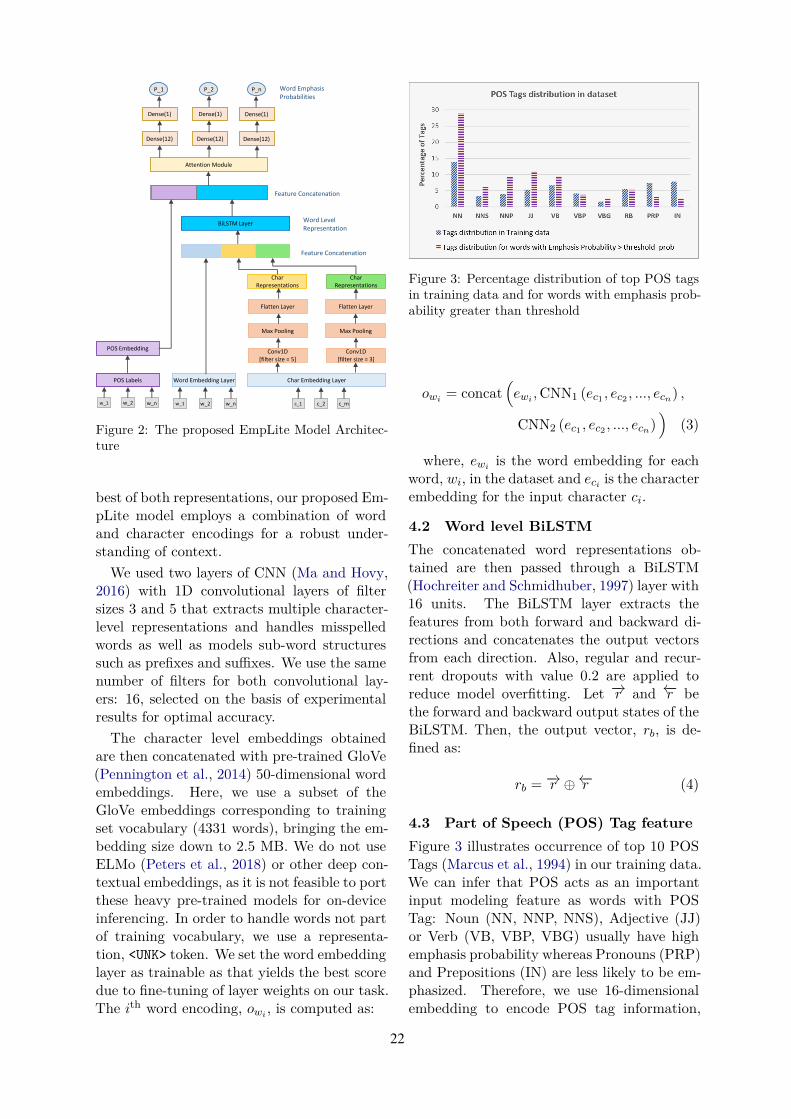
w_1 w_2 w_n c_1 c_2 c_m
Word Embedding Layer Char Embedding Layer
Conv1D [filter size = 5]
Conv1D [filter size = 3]
Max Pooling Max Pooling
Flatten Layer Flatten Layer
Char Representations
Char Representations
BiLSTM Layer
w_1 w_2 w_n
POS Labels
POS Embedding
Feature Concatenation
Word Level Representation
Feature Concatenation
Attention Module
Dense(12) Dense(12) Dense(12)
Dense(1) Dense(1) Dense(1)
p1 P_2P_1 P_n Word Emphasis Probabilities
Figure 2: The proposed EmpLite Model Architec-ture
best of both representations, our proposed Em-pLite model employs a combination of wordand character encodings for a robust under-standing of context.
We used two layers of CNN (Ma and Hovy,2016) with 1D convolutional layers of filtersizes 3 and 5 that extracts multiple character-level representations and handles misspelledwords as well as models sub-word structuressuch as prefixes and suffixes. We use the samenumber of filters for both convolutional lay-ers: 16, selected on the basis of experimentalresults for optimal accuracy.
The character level embeddings obtainedare then concatenated with pre-trained GloVe(Pennington et al., 2014) 50-dimensional wordembeddings. Here, we use a subset of theGloVe embeddings corresponding to trainingset vocabulary (4331 words), bringing the em-bedding size down to 2.5 MB. We do not useELMo (Peters et al., 2018) or other deep con-textual embeddings, as it is not feasible to portthese heavy pre-trained models for on-deviceinferencing. In order to handle words not partof training vocabulary, we use a representa-tion, <UNK> token. We set the word embeddinglayer as trainable as that yields the best scoredue to fine-tuning of layer weights on our task.The ith word encoding, owi , is computed as:
Figure 3: Percentage distribution of top POS tagsin training data and for words with emphasis prob-ability greater than threshold
owi = concat(ewi ,CNN1 (ec1 , ec2 , ..., ecn) ,
CNN2 (ec1 , ec2 , ..., ecn))
(3)
where, ewi is the word embedding for eachword, wi, in the dataset and eci is the characterembedding for the input character ci.
4.2 Word level BiLSTMThe concatenated word representations ob-tained are then passed through a BiLSTM(Hochreiter and Schmidhuber, 1997) layer with16 units. The BiLSTM layer extracts thefeatures from both forward and backward di-rections and concatenates the output vectorsfrom each direction. Also, regular and recur-rent dropouts with value 0.2 are applied toreduce model overfitting. Let −→r and ←−r bethe forward and backward output states of theBiLSTM. Then, the output vector, rb, is de-fined as:
rb =−→r ⊕←−r (4)
4.3 Part of Speech (POS) Tag featureFigure 3 illustrates occurrence of top 10 POSTags (Marcus et al., 1994) in our training data.We can infer that POS acts as an importantinput modeling feature as words with POSTag: Noun (NN, NNP, NNS), Adjective (JJ)or Verb (VB, VBP, VBG) usually have highemphasis probability whereas Pronouns (PRP)and Prepositions (IN) are less likely to be em-phasized. Therefore, we use 16-dimensionalembedding to encode POS tag information,
22

Table 3: Comparison of different model architectures
Model Model Size (MB) Matchm Average Scorem = 1 m = 2 m = 3 m = 4
Base: Word_Emb + BiLSTM + DenseLayer 1.10 0.479 0.639 0.731 0.785 0.659
Concat[LSTM(Char_Emb) +Word_Emb] + BiLSTM + Dense Layer 1.10 0.473 0.658 0.739 0.786 0.664
Concat[LSTM(Char_Emb) +Word_GloVe (Non-trainable)] + BiL-STM + Dense Layer
1.02 0.514 0.660 0.748 0.795 0.679
Concat[CNN(Char_Emb) + Word_GloVe(Non-trainable)] + BiLSTM + Dense Layer 1.04 0.523 0.669 0.754 0.801 0.687
Concat[CNN(Char_Emb) + Word_GloVe(Trainable)] + BiLSTM + Dense Layer 2.70 0.538 0.680 0.766 0.811 0.699
Concat[CNN1 (Char_Emb) + CNN2
(Char_Emb) + Word_GloVe (Train-able)] + BiLSTM + Dense Layer
2.77 0.528 0.690 0.771 0.810 0.701
Above Model + Attention 2.80 0.549 0.684 0.779 0.817 0.707
EmpLite: Above Model + POS FeatureConcatenation 2.82 0.541 0.698 0.782 0.823 0.711
which is concatenated with the output of theBi-LSTM layer (obtained from Equation 4):
−→h = concat (rb, epos) (5)
where, epos is the POS feature embeddingfor the sequence.
4.4 Attention LayerWe add the attention (Vaswani et al., 2017)layer to effectively capture prominent words inthe input text sequence. The attention weightis computed as the weighted sum of the outputof the previous layer, as shown below:
Z = softmax(wT
(tanh
(−→h1,−→h2, ...,
−→hi , ...,
−→hn
)))
(6)where, −→hi represents output vector of the
previous layer, and wT is the transpose of thetrained parameter vector.
The attention layer output is then passedthrough two time-distributed dense layerswith 12 and 1 units, respectively, with sigmoidactivation function to output emphasis proba-bility with respect to each word.
5 Experimental Settings & ResultsWe attempt numerous small changes to ourmodel to enhance the performance. Wechoose the hyperparameters to optimize ac-curacy while maintaining a small model size.
As the proposed solution is for mobile devices,we have also captured a system-specific met-ric, the model size in MB. We use the Tensor-flow framework (Abadi et al., 2016) for build-ing the models. Table 3 shows the comparisonof Matchm scores across different variants oflightweight models evaluated on test data.
The total number of trainable parametersvary in the range of 21,574 to 238,620 for allthe model results reported in Table 3. Wetrain the models with 32 batch-size and com-pile the model using Adam optimizer (Kingmaand Ba, 2014). We observe that using CNNgives a better score as compared to LSTM be-cause varying the size of kernels (3 and 5) andconcatenating their outputs allow the modelto detect patterns of multiple sizes.
We can also infer that using 50-dimensionalGloVe embeddings and setting it as trainableimproves the overall matching score. Thisis because we are utilizing language semanticknowledge acquired from the pre-trained em-beddings and then fine-tuning it for our task.However, there is an increase in model sizedue to more number of trainable parameters.Furthermore, we observe marginal gains in thematching score by adding POS tag as a featurefollowed by an attention layer as these help ina better identification of prominent keywordsbased on the context.
23

Figure 4: Emphasis Heatmap for test set samples with word probabilities from EmpLite
Table 4: Comparison with SOTA (Singhal et al.,2020)
Model Matchm Size (MB)IITK: BiLSTM + AttentionApproach 0.747 469.20
IITK: Transformers Approach 0.804 1536.00
EmpLite 0.716 2.82
Figure 4 presents the Emphasis Heatmap forsome examples from the test set using our fi-nal model. In Table 4 we benchmark our Em-pLite model with the state-of-the-art solutionby IITK (Singhal et al., 2020) which utilizedhuge pre-trained models like ELMo, BERT(Devlin et al., 2018), RoBERTa (Liu et al.,2019) and XLNet (Yang et al., 2019). Thesemodels require huge RAM/ROM for on-deviceinferencing making it unsuitable for edge de-vices where resources are constrained.
Table 5: Data Augmentation Analysis
Augmentation Dataset Matchm
Approach modified (%) ScoreNone 0 0.711
Word removal(≤1 per sentence)
20 0.70550 0.702100 0.716
Word removal(≥1 per sentence)
20 0.71150 0.70460 0.71270 0.705
Upper-casing a word 30 0.687
Reversing the sentence 10 0.704100 0.707
5.1 Data Augmentation AnalysisTable 5 shows that there is a little score gain byapplying data augmentation techniques. Foreach strategy, we experiment by applying the
augmentation approach to different percent-ages of the total training data and calculatedMatchm score. We observe that word upper-casing strategy results in a significant dropin the score due to model overfitting whereasword removal strategy (maximum 1 word persentence) on entire training data gives highestMatchm score of 0.716.
6 Conclusion
Modeling lightweight neural models that canrun on low-resource devices can greatly en-hance the end-user experience. In this work,we propose a novel, lightweight EmpLitemodel for text emphasis selection that can runon edge devices such as smartphones for choos-ing prominent words from short, informal text.We approach the emphasis selection problemas a sequence labeling task and multiple exper-iments have shown consistent improvement inthe accuracy. Our experimental results showthe impact of the attention layer and of usingPOS as an additional feature in boosting thematching score. Our best performing modelachieves an overall matching score of 0.716with a size of 2.82 MB, proving its effective-ness to run on low-resource edge devices.
Future work includes increasing the vocabu-lary with commonly used words in English andexploring thin versions of BERT like Distil-BERT (Sanh et al., 2019), MobileBERT (Sunet al., 2020b), and TinyBERT (Jiao et al.,2020) for modeling emphasis.
ReferencesMartín Abadi, Ashish Agarwal, Paul Barham, Eu-
gene Brevdo, Zhifeng Chen, Craig Citro, Greg SCorrado, Andy Davis, Jeffrey Dean, MatthieuDevin, et al. 2016. Tensorflow: Large-scale ma-
24

chine learning on heterogeneous distributed sys-tems. arXiv preprint arXiv:1603.04467.
Adobe. 2016. Adobe Spark. https://spark.adobe.com, accessed 2020-11-28.
Sarthak Anand, Pradyumna Gupta, HemantYadav, Debanjan Mahata, Rakesh Gosangi,Haimin Zhang, and Rajiv Ratn Shah. 2020. Mi-das at semeval-2020 task 10: Emphasis selectionusing label distribution learning and contextualembeddings. arXiv preprint arXiv:2009.02619.
Jacob Devlin, Ming-Wei Chang, Kenton Lee, andKristina Toutanova. 2018. Bert: Pre-training ofdeep bidirectional transformers for language un-derstanding. arXiv preprint arXiv:1810.04805.
Sepp Hochreiter and Jürgen Schmidhuber. 1997.Long short-term memory. Neural Comput.,9(8):1735–1780.
Zhengjie Huang, Shikun Feng, Weiyue Su, XuyiChen, Shuohuan Wang, Jiaxiang Liu, XuanOuyang, and Yu Sun. 2020. Ernie at semeval-2020 task 10: Learning word emphasis selectionby pre-trained language model. arXiv preprintarXiv:2009.03706.
Xiaoqi Jiao, Yichun Yin, Lifeng Shang, Xin Jiang,Xiao Chen, Linlin Li, Fang Wang, and QunLiu. 2020. TinyBERT: Distilling BERT for nat-ural language understanding. In Findings ofthe Association for Computational Linguistics:EMNLP 2020, pages 4163–4174, Online. Associ-ation for Computational Linguistics.
Hyeon Gyu Kim. 2020. Efficient keyword extrac-tion from social big data based on cohesion scor-ing. Journal of the Korea Society of Computerand Information, 25(10):87–94.
Diederik P Kingma and Jimmy Ba. 2014. Adam:A method for stochastic optimization. arXivpreprint arXiv:1412.6980.
Dongyun Liang, Weiran Xu, and Yinge Zhao. 2017.Combining word-level and character-level repre-sentations for relation classification of informaltext. In Proceedings of the 2nd Workshop onRepresentation Learning for NLP, pages 43–47.
Marina Litvak and Mark Last. 2008. Graph-basedkeyword extraction for single-document summa-rization. In Coling 2008: Proceedings of theworkshop Multi-source Multilingual InformationExtraction and Summarization, pages 17–24.
Yinhan Liu, Myle Ott, Naman Goyal, JingfeiDu, Mandar Joshi, Danqi Chen, Omer Levy,Mike Lewis, Luke Zettlemoyer, and VeselinStoyanov. 2019. Roberta: A robustly opti-mized bert pretraining approach. arXiv preprintarXiv:1907.11692.
Xuezhe Ma and Eduard Hovy. 2016. End-to-endsequence labeling via bi-directional lstm-cnns-crf. arXiv preprint arXiv:1603.01354.
Mitchell Marcus, Grace Kim, Mary AnnMarcinkiewicz, Robert MacIntyre, Ann Bies,Mark Ferguson, Karen Katz, and Britta Schas-berger. 1994. The penn treebank: Annotatingpredicate argument structure. In Proceedings ofthe Workshop on Human Language Technology,HLT ’94, page 114–119, USA. Association forComputational Linguistics.
Yutaka Matsuo and Mitsuru Ishizuka. 2004. Key-word extraction from a single document us-ing word co-occurrence statistical information.International Journal on Artificial IntelligenceTools, 13(01):157–169.
MonkeyLearn. 2020. Keyword Extraction: AGuide to Finding Keywords in Text. https://monkeylearn.com/keyword-extraction/, accessed2020-07-03.
NEON. 2020. NEON. https://www.neon.life/, ac-cessed 2020-06-24.
Jeffrey Pennington, Richard Socher, and Christo-pher Manning. 2014. GloVe: Global vectorsfor word representation. In Proceedings of the2014 Conference on Empirical Methods in Natu-ral Language Processing (EMNLP), pages 1532–1543, Doha, Qatar. Association for Computa-tional Linguistics.
Matthew E Peters, Mark Neumann, Mohit Iyyer,Matt Gardner, Christopher Clark, Kenton Lee,and Luke Zettlemoyer. 2018. Deep contextu-alized word representations. arXiv preprintarXiv:1802.05365.
Wisdom Quotes. 2020. Wisdom Quotes - Getwiser slowly. https://wisdomquotes.com, ac-cessed 2020-11-30.
RiTUAL-UH. 2020. SemEval2020 Task10 Empha-sis Selection. https://github.com/RiTUAL-UH/SemEval2020_Task10_Emphasis_Selection, ac-cessed 2020-11-22.
Stuart Rose, Dave Engel, Nick Cramer, and WendyCowley. 2010. Automatic keyword extractionfrom individual documents. Text mining: ap-plications and theory, 1:1–20.
Victor Sanh, Lysandre Debut, Julien Chaumond,and Thomas Wolf. 2019. Distilbert, a distilledversion of bert: smaller, faster, cheaper andlighter. arXiv preprint arXiv:1910.01108.
shallowLearner. 2020. SemEval 2020 - Task10: Emphasis Selection For Written Text inVisual Media. https://competitions.codalab.org/competitions/20815, accessed 2020-08-15.
25

Amirreza Shirani, Franck Dernoncourt, PaulAsente, Nedim Lipka, Seokhwan Kim, JoseEchevarria, and Thamar Solorio. 2019. Learn-ing emphasis selection for written text in visualmedia from crowd-sourced label distributions.In Proceedings of the 57th Annual Meeting ofthe Association for Computational Linguistics,pages 1167–1172.
Vipul Singhal, Sahil Dhull, Rishabh Agarwal, andAshutosh Modi. 2020. Iitk at semeval-2020 task10: Transformers for emphasis selection. arXivpreprint arXiv:2007.10820.
Yu Sun, Shuohuan Wang, Yu-Kun Li, Shikun Feng,Hao Tian, Hua Wu, and Haifeng Wang. 2020a.Ernie 2.0: A continual pre-training frameworkfor language understanding. In AAAI, pages8968–8975.
Zhiqing Sun, Hongkun Yu, Xiaodan Song, Ren-jie Liu, Yiming Yang, and Denny Zhou. 2020b.Mobilebert: a compact task-agnostic bertfor resource-limited devices. arXiv preprintarXiv:2004.02984.
Ashish Vaswani, Noam Shazeer, Niki Parmar,Jakob Uszkoreit, Llion Jones, Aidan N Gomez,Łukasz Kaiser, and Illia Polosukhin. 2017. At-tention is all you need. Advances in neural in-formation processing systems, 30:5998–6008.
Zhilin Yang, Zihang Dai, Yiming Yang, Jaime Car-bonell, Russ R Salakhutdinov, and Quoc V Le.2019. Xlnet: Generalized autoregressive pre-training for language understanding. In Ad-vances in neural information processing systems,pages 5753–5763.
Chengzhi Zhang. 2008. Automatic keyword extrac-tion from documents using conditional randomfields. Journal of Computational InformationSystems, 4(3):1169–1180.
Kuo Zhang, Hui Xu, Jie Tang, and Juanzi Li. 2006.Keyword extraction using support vector ma-chine. In international conference on web-age in-formation management, pages 85–96. Springer.
26

Proceedings of the ICON 2020 Workshop on Joint NLP Modelling for Conversational AI, pages 27–32Patna, India, December 18 - 21, 2020. ©2020 NLP Association of India (NLPAI)
Named Entity Popularity Determination using Ensemble Learning
Vikram KarthikeyanDepartment of ISE
BMS College of EngineeringBangalore, India
B Shrikara VarnaDepartment of ISE
BMS College of EngineeringBangalore, India
Amogha HegdeDDepartment of ISE
BMS College of EngineeringBangalore, India
Govind SatwaniDepartment of ISE
BMS College of EngineeringBangalore, India
Ranjan SamalDepartment of Multimodal NLP
Samsung R&D InstituteBangalore, India
Shambhavi B RDepartment of ISE
BMS College of EngineeringBangalore, India
Jayarekha PDepartment of ISE
BMS College of EngineeringBangalore, India
Abstract
Determining the popularity of a Named En-tity after completion of Named Entity Recogni-tion (NER) task finds many applications. Themost popular of them being virtual assistantswhere disambiguating entities without contex-tual help is crucial. A single named entitycould belong to multiple domains, making itnecessary for the popularity determination ap-proach to give accurate results. The more ac-curate results can be used to improve the func-tioning of virtual assistants. This work stud-ies disambiguation of Named Entities (NE) ofMusic and Movie domains and resolves popu-larity considering relevant features like region,movie/music awards, album count, run timeetc. Decision Trees and Random Forests ap-proaches are applied on the dataset and the lat-ter ensemble learning algorithm resulted in ac-ceptable accuracy.
1 Introduction
Over the years the use of electronic devices for var-ious tasks and services have become predominant.These days, services such as E-commerce, videoand music streaming over the internet are common.Thus, it is crucial that these services provide theusers with what they require and also give rele-vant recommendations. Moreover, search enginesshould know what results to show based not only onthe query string but also consider other factors likedemographic, geographic location, user’s searchhistory, etc. Identifying entities in a query string istermed as Named Entity Recognition (NER). Dueto the vast and diverse collection of data, NERsometimes alone may not be sufficient. In suchcases Name Entity Popularity Detection can beused to prioritize results which may be more rel-
27

evant to the user based on various factors. Thisis especially used while designing a conversationsmart assistant, to provide the user with the bestresults. For example, if the user asks the virtualassistant to “play wolves” then it has to decidewhether to play the song wolves or play the moviewolves without any given context or sentence asso-ciated with. In such a scenario information aboutthe user’s search history has conventionally beenused to resolve the ambiguity and judge what theuser really wanted. This process of using data otherthan the query string to disambiguate between enti-ties with similar names is known as Named EntityPopularity Determination (NEPD). Our objectiveis to accomplish this task without considering userhistory.
2 Problem Statement
NEPD aims at determining the popularity of theNamed Entities. This approach can be extendedfor use in Conversation Smart Assistants, helpingthe application to understand user speech, disam-biguate entities and give the best search results.NEPD involves primarily
• Data Mining of features which help to deter-mine the popularity of the target NE.
• Designing an algorithm to predict the pop-ularity from the mined features for variousdomains. Music and Movie domains are con-sidered in our work.
3 Related Work
Several approaches have been put forward to getbetter results for NER. Some of these methods in-volve the use of neural architectures in addition toBi-LSTM methods. Lample et al. (2016) has devel-oped a method based on transition-based parsingand stack-LSTMs. Building on the approach ofensemble learning for NER, multiple approacheshave been combined to obtain a better result (Speckand Ngomo, 2014). The results of various classifieralgorithms were integrated (Florian et al., 2003),resulting in significant strides in NER performance.
In the work of (Cucerzan, 2007), information ex-tracted from Wikipedia is stored in two databases,and the entities are mapped together. After entitymappings, a disambiguation component is used forNamed Entity Disambiguation (NED). To improvethe performance of NED, in addition to Bi-LSTM;other models that use GCN and RNN, along with
Figure 1: Correlation Matrix of the features
attention have also been experimented upon (Ce-toli et al., 2018). Combining graphs and popularityranking into a single model is another approachtowards NED (Alhelbawy and Gaizauskas, 2014) ,(Han and Zhao, 2010), where graphs, knowledgebases, are used for Entity Generation, Entity rank-ing and NED. Joint Embeddings have also beenused for improving the results for NED (Yamadaet al., 2016).
To enhance the results of the NER models, En-tity Popularity models have been proposed (Govaniet al., 2013), (Blanco et al., 2013). These mod-els use the personal history of the user, create aranking of entities, and have resulted in recom-mendations that are more likely and specifically re-lated to the concerned user. The ranking of entitieshas been improved by increasing the performanceof the Language Model (LM), during AutomaticSpeech Recognition (Van Gysel et al., 2020). Themodel used for predicting entity popularity in thispaper resulted in improvements of 20% in worderror rate.
4 Dataset and Feature Extraction
The next step in dealing with the sparseness wasbuilding the correlation and covariation matrix.Thecorrelation matrix, shown in Figure1 helped decidewhich features to drop, and which features to retain,to get a better clarity of the data we had collected.
The initial dataset of entities and the domains towhich they are to be classified into movie/music
28

Feature Name Description SouceType Genre (applicable to musicians,songs and
movies only, and not to actressIMDb, MusicBrainz
Count of Movies Acted The number of movies a person has actedin (i a significant role)
IMDb
Count of Movies Directed Some artists tend to direct themovies they work in.
IMDb
tCount of Movies Produced Some artists tend to produce the moviesthey work in. Also includes the number ofalbums that are self produced by an artist.
IMDb
Release Date The time description of when a particularsong or movie was released. It helps in de-termining the popularity of that particularwork in that decade.
IMDb, MusicBrainzand Last.fm
Region Place of release of the movie or album orlocation of concert also refers to the regionwhere an artist is based.
IMDb
Count of Albums The higher the number, the more weigh-tage for music domain
Last.fm API
cCount of Concerts The number of live concerts held by theparticular artist
Last.fm API
Count of Movie Awards The number of awards a particular personhas in a domain
IMDb
Count of Music Awards The number of awards a particular personhas in a domain
IMDb, MusicBrainz
Run Time Sum of durations of all the songs releasedby the person
MusicBrainz
Table 1: Features and their description.
was generated. Considering the domains in theproblem statement, a list of applicable featuresalong with the source from which the data for thatparticular feature can/could be extracted was made.This decision was based on the considerations thata person who is active predominantly in one ofthe two domains, will have a higher value for thefeatures pertaining to that domain. Additionally,people who are active in both the domains will havevalues for all the features but some comparativelyhigher than the other. The list of features is givenin Table 1.
The problem at hand is finding the popularityof a person in the domain and identification of thedomain in which the person is more popular if theperson has an existence in both. The idea behindthe selection of a feature was based on this problem.The popularity of any person in a domain is basedon the works of that person, and the accolades theperson has received for their work in the particularfield. The feature “Run Time” was included in par-
ticular as some of the artists voice for songs in themovies they have acted in. And hence they mighthave a considerable number of songs under them.This feature will help us to distinguish between afull-fledged singer (music domain) and actors whojust give voice for a song in a movie.
The data was collected and a .csv file was formed.Most of the entities in the given dataset were disam-biguous, and hence the data collected was sparse asthe entity was inclined to one of the domains. Toovercome this problem of sparseness, the datasetwas first divided into two-parts: one file contain-ing the entities that were the names of the peopleand/or music bands, while the other contained theentities that were the names of the artwork (movieand/or song tracks). Dividing the single file intotwo, helped deal with the sparseness a bit as someof the features that were not applicable to that par-ticular category were removed.
There were many challenges in handling the art-work file. Many artworks pertaining to the same
29
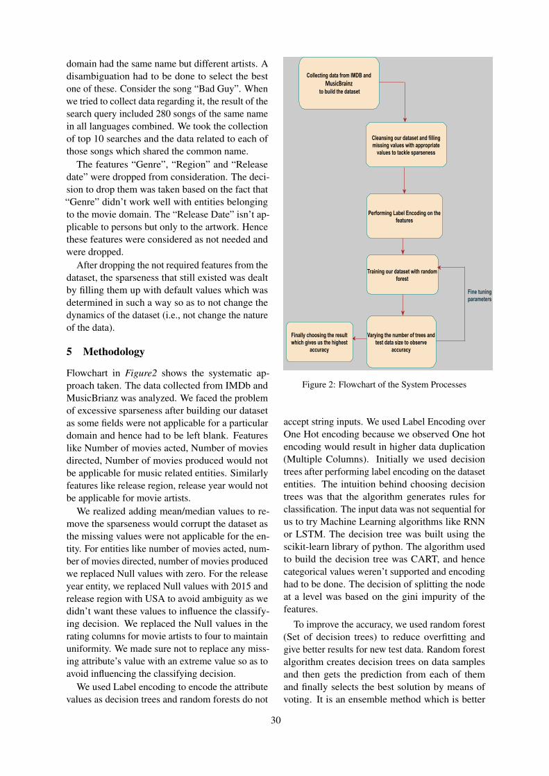
domain had the same name but different artists. Adisambiguation had to be done to select the bestone of these. Consider the song “Bad Guy”. Whenwe tried to collect data regarding it, the result of thesearch query included 280 songs of the same namein all languages combined. We took the collectionof top 10 searches and the data related to each ofthose songs which shared the common name.
The features “Genre”, “Region” and “Releasedate” were dropped from consideration. The deci-sion to drop them was taken based on the fact that“Genre” didn’t work well with entities belongingto the movie domain. The “Release Date” isn’t ap-plicable to persons but only to the artwork. Hencethese features were considered as not needed andwere dropped.
After dropping the not required features from thedataset, the sparseness that still existed was dealtby filling them up with default values which wasdetermined in such a way so as to not change thedynamics of the dataset (i.e., not change the natureof the data).
5 Methodology
Flowchart in Figure2 shows the systematic ap-proach taken. The data collected from IMDb andMusicBrianz was analyzed. We faced the problemof excessive sparseness after building our datasetas some fields were not applicable for a particulardomain and hence had to be left blank. Featureslike Number of movies acted, Number of moviesdirected, Number of movies produced would notbe applicable for music related entities. Similarlyfeatures like release region, release year would notbe applicable for movie artists.
We realized adding mean/median values to re-move the sparseness would corrupt the dataset asthe missing values were not applicable for the en-tity. For entities like number of movies acted, num-ber of movies directed, number of movies producedwe replaced Null values with zero. For the releaseyear entity, we replaced Null values with 2015 andrelease region with USA to avoid ambiguity as wedidn’t want these values to influence the classify-ing decision. We replaced the Null values in therating columns for movie artists to four to maintainuniformity. We made sure not to replace any miss-ing attribute’s value with an extreme value so as toavoid influencing the classifying decision.
We used Label encoding to encode the attributevalues as decision trees and random forests do not
Collecting data from IMDB andMusicBrainz
to build the dataset
Cleansing our dataset and fillingmissing values with appropriate
values to tackle sparseness
Performing Label Encoding on thefeatures
Training our dataset with randomforest
Varying the number of trees andtest data size to observe
accuracy
Steps showing the approach taken
Finally choosing the resultwhich gives us the highest
accuracy
Fine tuningparameters
Figure 2: Flowchart of the System Processes
accept string inputs. We used Label Encoding overOne Hot encoding because we observed One hotencoding would result in higher data duplication(Multiple Columns). Initially we used decisiontrees after performing label encoding on the datasetentities. The intuition behind choosing decisiontrees was that the algorithm generates rules forclassification. The input data was not sequential forus to try Machine Learning algorithms like RNNor LSTM. The decision tree was built using thescikit-learn library of python. The algorithm usedto build the decision tree was CART, and hencecategorical values weren’t supported and encodinghad to be done. The decision of splitting the nodeat a level was based on the gini impurity of thefeatures.
To improve the accuracy, we used random forest(Set of decision trees) to reduce overfitting andgive better results for new test data. Random forestalgorithm creates decision trees on data samplesand then gets the prediction from each of themand finally selects the best solution by means ofvoting. It is an ensemble method which is better
30

than a single decision tree because it reduces theover-fitting by averaging the result and improvesthe classification accuracy.
6 Experimental Results
On analyzing our dataset, we decided that a ma-chine learning approach would work well for theproblem in hand. We initially used decision treesand achieved an accuracy of 86%. Figure3 rep-resents the decision tree that was built using theCART algorithm. The split of nodes at each levelis depicted along with its Gini impurity value.
Figure 3: Decision Tree generated
Algorithm Test Data(%)
TrainingData (%)
Accuracy(%)
DecisionTree
20 80 86
RandomForest
20 80 89
RandomForest
30 70 93
RandomForest
40 60 94.3
Table 2: Experimental Results.
To increase the accuracy of classification and pre-vent overfitting we decided to use random forest.
Using the random forest, we obtained an accuracyof 89%. As our dataset was relatively small, in-creasing the number of trees for random forest didnot yield us with better accuracy, so we increasedthe test data size to have larger data to classify from20% to 40%. Results are tabulated in Table 2. Fi-nally, we achieved an accuracy of 94.3% percentusing random forest with 100 trees.
7 Conclusion
The problem of Named Entity Popularity Deter-mination was to be solved without any contextualdata or user history in the domains of music andmovies. In virtual assistants, users usually giveonly named entity without context or a statementassociated with it. We built our customized datasetfrom IMDb and MusicBrainz. The issue of exces-sive sparseness was solved by filling the missingvalues in the dataset with generic relevant valuesand made sure it wouldn’t influence the classifyingdecision. With decision trees, an accuracy of 86%was achieved. To improve the accuracy and preventoverfitting random forests was used. We finallyachieved an accuracy of 94.3%. The approach usedhere to disambiguate ambiguous entities can beextended to other related domains like TV Shows,Podcasts and Radios by collecting relevant features.This approach can be modelled to disambiguate am-biguous entities between various related domainswithout contextual information.
ReferencesAyman Alhelbawy and Robert Gaizauskas. 2014.
Graph ranking for collective named entity disam-biguation. In Proceedings of the 52nd Annual Meet-ing of the Association for Computational Linguistics(Volume 2: Short Papers), pages 75–80.
Roi Blanco, Berkant Barla Cambazoglu, Peter Mika,and Nicolas Torzec. 2013. Entity recommendationsin web search. In International Semantic Web Con-ference, pages 33–48. Springer.
Alberto Cetoli, Mohammad Akbari, Stefano Bragaglia,Andrew D O’Harney, and Marc Sloan. 2018. Namedentity disambiguation using deep learning on graphs.arXiv preprint arXiv:1810.09164.
Silviu Cucerzan. 2007. Large-scale named entity dis-ambiguation based on wikipedia data. In Proceed-ings of the 2007 joint conference on empirical meth-ods in natural language processing and computa-tional natural language learning (EMNLP-CoNLL),pages 708–716.
31

Radu Florian, Abe Ittycheriah, Hongyan Jing, andTong Zhang. 2003. Named entity recognitionthrough classifier combination. In Proceedings ofthe seventh conference on Natural language learn-ing at HLT-NAACL 2003, pages 168–171.
Tabreez Govani, Hugh Williams, Jamie Buckley, NitinAgrawal, Andy Lam, and Kenneth A Moss. 2013.Determining entity popularity using search queries.US Patent 8,402,031.
Xianpei Han and Jun Zhao. 2010. Structural semanticrelatedness: a knowledge-based method to namedentity disambiguation. In Proceedings of the 48thAnnual Meeting of the Association for Computa-tional Linguistics, pages 50–59.
Guillaume Lample, Miguel Ballesteros, Sandeep Sub-ramanian, Kazuya Kawakami, and Chris Dyer. 2016.Neural architectures for named entity recognition.arXiv preprint arXiv:1603.01360.
Rene Speck and Axel-Cyrille Ngonga Ngomo. 2014.Ensemble learning for named entity recognition. InInternational semantic web conference, pages 519–534. Springer.
Christophe Van Gysel, Manos Tsagkias, ErnestPusateri, and Ilya Oparin. 2020. Predicting entitypopularity to improve spoken entity recognition byvirtual assistants. arXiv preprint arXiv:2005.12816.
Ikuya Yamada, Hiroyuki Shindo, Hideaki Takeda, andYoshiyasu Takefuji. 2016. Joint learning of the em-bedding of words and entities for named entity dis-ambiguation. arXiv preprint arXiv:1601.01343.
32

Proceedings of the ICON 2020 Workshop on Joint NLP Modelling for Conversational AI, pages 33–39Patna, India, December 18 - 21, 2020. ©2020 NLP Association of India (NLPAI)
Optimized Web-Crawling of Conversational Data from Social Media andContext-Based Filtering
Annapurna P PatilDepartment of Computer Science
and EngineeringRamaiah Institute of Technology
Bangalore, [email protected]
Gaurav KarkalDepartment of Computer Science
and EngineeringRamaiah Institute of Technology
Bangalore, [email protected]
Jugal WadhwaDepartment of Computer Science
and EngineeringRamaiah Institute of Technology
Bangalore, [email protected]
Meer SawoodDepartment of Computer Science
and EngineeringRamaiah Institute of Technology
Bangalore, [email protected]
Rajarajeswari SDepartment of Computer Science
and EngineeringRamaiah Institute of Technology
Bangalore, [email protected]
Keerthana PurushothamDepartment of Computer Science
and EngineeringRamaiah Institute of Technology
Bangalore, [email protected]
K Dhanush ReddyDepartment of Computer Science
and EngineeringRamaiah Institute of Technology
Bangalore, [email protected]
Abstract
Building Chatbot’s requires a large amountof conversational data. In this paper, aweb crawler is designed to fetch multi-turndialogues from websites such as Twit-ter, YouTube and Reddit in the form ofa JavaScript Object Notation (JSON) file.Tools like Twitter Application ProgrammingInterface (API), LXML Library, and JSONlibrary are used to crawl Twitter, YouTubeand Reddit to collect conversational chat data.The data obtained in a raw form cannot beused directly as it will have only text metadatasuch as author or name, time to provide moreinformation on the chat data being scraped.The data collected has to be formatted fora good use case, and the JSON library ofpython allows us to format the data easily. Thescraped dialogues are further filtered basedon the context of a search keyword without
introducing bias and with flexible strictness ofclassification.
1 Introduction
Real-world data remains a necessary part of train-ing system models. The digital streams that indi-viduals produce are quite useful in the Data Anal-ysis domain, like natural language processing andmachine learning. Social networking applicationslike Twitter, YouTube and Reddit contain a largevolume of data that are quite useful for various al-gorithms. Naturally, the need to make informationeasily accessible to all leads to deploying a conver-sational agent. In order to build a chat model, ahuge volume of conversational text data is required.
Twitter is a microblogging service that allowsindividuals to post short messages called tweets
33

that appear on timelines. These tweets were limitedto 140 characters, which has been later expandedto 280 characters and prone to change again in thefuture. Tweets consist of two kinds of metadatathat are entities and places. Tweet entities are hash-tags, user- mentions, images, and places in the realworld’s geographical locations. Metadata and shortprose add to fewer than 280 characters can link toWebpages, Twitter users. Twitter timelines are cat-egorized into the home timeline and user timeline.Timelines are collections of tweets in chronologi-cal order. Twitter API uses Representational StateTransfer (REST) API to crawl and collect a randomset of sample public tweets. The API allows usersto explore and search for trending topics, tweets,hashtags, and geographical locations.
YouTube, a video-sharing website, allowsusers to view, upload, rate, report on videos. Itcontains a wide variety of videos such as TV showclips, music videos, documentaries. It also providesa platform for users to communicate and describetheir thoughts about what they watch through com-ments.
Reddit is a social news platform where regis-tered users may submit links, images, text, postsand also upvote or downvote the posts posted byother users. Posts are organized based on boardscreated by the user called subreddit. It is also aplatform for web content rating and discussions.Reddit stores all of its content in json format whichcan be viewed on the browser by extending thereddit link with the extension ’.json’.
Real-time datasets are needed to build a modelto generate accurate output. As the availabledatasets are insufficient and do not contain real-istic examples, there is a need to build a crawlerwhich would scrape conversational data. Buildingcrawlers for each website would allow collection ofconversational data. This would help in the creationof datasets of conversational data.
2 Literature Survey
A Focused crawler is designed to crawl and retrievespecific topics of relevance. The idea of the focusedcrawler is to selectively look for pages that arerelevant while traversing and crawling the leastnumber of irrelevant pages on the web.
Context Focused Crawlers (CFC) use a lim-ited number of links from a single queried docu-ment to obtain all relevant pages to the document,and the said obtained documents are relevant con-
cerning the context. This data obtained is then usedto train a classifier that would detect the contextof documents and allow classification of them intocategories based on the link distance from a queryto target. Features of a crawler are-
• Politeness
• Speed
• Duplicate Content
Each website comes with the inclusion of afile known as robot.txt. It is a standardized prac-tice where robots or bots are communicated withthe website through this protocol. This standardprovides the necessary instructions to the crawlerabout the status of the website and whether it is al-lowed to scrape the data off of the website. This isused to inform crawlers whether the website can becrawled either partially or fully, if the website can-not be crawled as per the robot.txt then the serverblocks any such requests and can even lead to block-ing of IP’s.
Websites have robot.txt, which prevent theuse of crawlers that attempt to scrape large datafrom their website. Any request for a large amountof data is blocked almost immediately. To pre-vent such a case where the crawler should not beblocked, a list of publicly available proxy serversas described in Achsan (2014) is used to scale andcrawl the website. Twitter is a popular social me-dia platform used for communication. Crawlingsuch a website can be useful to gain conversationaldata, and such information can be targeted basedon the topic; one such example is a perception onthe internet of things as shown in Bian J (2017) orAssessing the Adequacy of Gender IdentificationTerms on Intake Forms as described in Hicks A(2015).
3 Proposed System
3.1 Twitter Crawler
Twitter API provides the tweets encoded in JSONformat. The JSON format contains key-value pairsas the attributes along with their values. Twitterhandles both the users and as well the tweets asobjects. The user object contains attributes includ-ing their name, geolocation, followers. The tweetobject contains the author, message, id, timestamp,geolocation etc. The JSON file can also containadditional information in the media or links present
34

in the tweets, including the full Uniform ResourceLocator(URL) or link’s title or description.
Each tweet object contains various child ob-jects. It contains a User object describing the au-thor of the object, a place object if the tweet isgeo-tagged, and entities object, which is an arrayof URLs, hashtags, etc. Extended tweets includetweets with longer text fields exceeding 140 charac-ters. It also contains a complete list of entities likehashtags, media, links, etc. They are identified bythe Boolean truncated field equals true, signifyingthe extended tweet section to be parsed instead orthe regular section of the tweet object.
The retweet object contains the retweet objectitself as well as the original tweet object. This iscontained in the retweeted status object. Retweetscontain no new data or message, and the geoloca-tion and place is always null. A retweet of anotherretweet will still point to the original tweet.
Quote tweets contain new messages alongwith retweeting the original tweet. It can also con-tain a new set of media, links or hashtags. It con-tains the tweet being quoted in the quoted statussection. It also contains the User object of theperson quoting the tweet.
The Twitter REST API method gives accessto core Twitter data. This includes update timelines,status data, and user information. The API methodsallow interaction with Twitter Search and trendsdata.
The Twitter streaming API obtains a set ofpublic tweets based upon search phrases, user IDsas well as location. It is equipped to handle GETand POST requests as well. However, there is alimitation on the number of parameters specifiedby GET to avoid long URLs. Filters used with thisAPI are-
• follow- user IDs of whom to fetch the statuses
• track- specific words to be searched for.
• location- filter tweets based on geo location.
Workflow of Twitter Crawler:
1. Crawling for public tweets
This project uses Streaming API access tocrawl and collect a random sample set ofpublic tweets. These tweets are crawled inreal time. These tweets can be filtered withgeo location to crawl tweets with respect to aspecific region. These sample sets of public
tweets are outputted to a json file as seen inFigure 1.
Figure 1: The above figure depicts a tweet object. Itcontains all attributes contained within a tweet
2. Crawling for tweets while searching and mon-itoring a list of keyword
For searching and monitoring, a list of key-words, search/tweets is used. Streaming API’sstatus/filters are not used as it does not pro-vide previous tweets at all. Search/tweets areused to crawl and provide tweets from at mosta week back. This function continues to end-lessly crawl for tweets matching the query.Another advantage of using this method isthat it does not limit the number of keywordsit can track, unlike statuses/filters, which re-quire separate or new instances to search fordifferent keywords.
3. Filtering Tweets with replies
The crawler filters through the collected pub-lic sample of tweets to find specific tweetswith replies. It finds the same by checkingthe ’in reply to status id’ attribute of the col-lected tweets. It then proceeds to crawl theparent tweet using the ’in reply to status id’.It outputs the parent and the reply tweet to-gether in the JSON file, as seen in Fig. 2.
4. Filtering Quoted Retweets
Quoted Retweets or retweets with com-ments are filtered from the collected set of
35

public tweets. This is achieved by pars-ing the collected tweets and searching for’quoted status’. The parent tweet is con-tained within the quoted retweet inside the’quoted status’ attribute. The crawler outputsthe quoted retweet with its contained parenttweet to the JSON file, as seen in Fig. 3.
Figure 2: In the above diagram, the ’in reply to status’tag used to filter the tweets is highlighted.
3.2 Youtube Crawler
Cascading Style Selector and Python are the pri-mary tools that are used. The crawler works toaccept a CSS selector expression as input; the se-lector compiles to XPath, and many other librariessuch as requests.
AJAX interchanges data with the server inthe background enabling the web page to be up-dated. This allows certain sections to be up-dated as opposed to the entire page. Python is anobject-oriented programming language for general-purpose programming. It helps enhance code read-ability by including the whitespace.
YouTube has server-side rendering with au-tomation,it is impractical to wait for all commentsto get loaded in order to extract them. This workuses the fact that YouTube sends an AJAX Request
Figure 3: In the above diagram, the ’quoted status’ tagused to filter the tweets is highlighted.
to a URL in order to get comments. By using thatURL, the crawler makes a session with a user agentand sends the AJAX request to the server for aparticular video id input given by the user; all thecomments are downloaded and stored in a JSONformat; each comment and its reptiles are identifiedby the id it has, replies have the id of the maincomment prefixed with its id.
Figure 4: Algorithm Crawl Youtube Comments
3.3 Reddit Crawler
Reddit is a social media platform that serves thepurpose of sharing the content of many forms, in-cluding multimedia content. A subreddit is definedto cover a topic of interest, for example, sportsand users can make posts on sports, and others cancomment on these posts.
Usually, scraping Reddit is difficult since Red-
36

dit easily blocks IP addresses after a certain numberof requests. Hence the work done focuses on view-ing Reddit pages as a collection of JSON objectsthat can be simply parsed for the required contenttype. This overcomes the issue mentioned aboveof having a single IP address blocked at multiplerequests.
Reddit returns a JSON object when the link isextended with ’.json’, which is passed as an initialrequest to crawl, and a callback function is calledwith the response downloaded from the request. Inthe callback function, the response object is parsed,and the crawler retrieves the comments. Post linksare retrieved based on the search term entered andsorted on hot, new, top, rising, or controversial.The number of post links is limited based on thelimit factor. Each of these posts contains a setof permalinks containing information about thecomments. Each of these permalinks is parsed, aretraversed, and a JSON object is retrieved. ObtainedJSON objects are parsed to retrieve the comments.
Scrapy, a web scraping framework, is usedto extract structured content from the Reddit page.Libraries such as JSON, time are used. The JSONlibrary provided by python is used to parse JSONobjects returned from Reddit links. The crawleroutput can be seen as in Fig. 5.
Figure 5: Crawler output in JSON format
4 Context Based Dialogue Filtering
The tool used in the comment filtering module ispython libraries centered around handling and ma-nipulating the data obtained from the crawlers. Thefiltering model uses the pandas’ library to read theraw data from a .csv form of the output json datafrom the crawlers. The filtering model uses thenltk library to clean our data, tokenize the data, andremove stop words.
The outputs collected from the crawlers areall initially in JSON files. These are then convertedinto a uniformly structured csv type file. The maintechnology used is in the form of the bag of wordsmodel used to analyze the importance of each gen-erated token within the context of the extracteddata.
In the implementation, note that input is thecsv file, and output is a cleaned and appended list ofcomments and replies. The comments and repliesare first to read into a data frame following whichthe following cleaning methods are applied: Con-vert to lowercase “[/()\[\]\—@,;” symbols are re-placed by a space “0-9a-z + ” symbols are removed
Stopwords are removed according to the ’En-glish’ stopwords from the nltk stopwords library
The first 30 comments are then analyzed togenerate a list of tokens, and their frequencies arecounted. Tokens with ”” are given high preference,and a high-frequency list of words is taken as a sub-set of the original list. Then all the comments andreplies from the data frame are cross-referenced.Entries that do not contain any of the words in thelist of high-frequency words are rejected. The re-maining entries which have been filtered are theoutput.
Figure 6: Algorithm Comment filtering
37

5 Analysis and Comparison
5.1 TwitterStandard twitter crawlers use the Streaming APIstatues/filters, which do not provide old tweets. Theother caveat is that it can only track a limited num-ber of keywords. So, if the user has a lot to track,he will need to have many separate instances, eachtracking different parts of the keywords.
The proposed Twitter crawler is beneficialin that it uses search/tweets to get old tweets. Itsearches for a portion of the keyword list at a time.The Streaming API is used to collect a random sam-ple of real-time public teams. The REST API isused to filter and obtain tweets with respect to spec-ified filters. The implemented algorithm filters thetweets to obtain tweets relevant to conversationaldata.
5.2 YouTubeSelenium, a vast tool for scraping, can crawlYouTube. YouTube has server-side rendering,which loads the website first upon which it can bescraped for data. This approach’s problem is thatthe website has to be loaded upon which JavaScripthas to be used to load more comments on the webpage.
The novelty in this approach lies inthat by analyzing how YouTube retrieved itscomments, and the same approach can beused by sending AJAX requests to the URLhttps://youtube.com/id/comments. Since sectionsof the page that does not include comments are notdownloaded, the crawler saves time and resourcesover the downloaded contents.
5.3 RedditReddit being a dynamic website and communicatesthrough rest API; selenium is a powerful web scrap-ing tool that can be used to scrape dynamic web-sites. While simulating the browser, crawlers canmimic the scrolling of the pages, clicking to readmore comments. Since the speed of retrieval willdepend on the speed at which each section of thepage loads, it is inefficient as the next load will onlystart after the previous load and the cursor scrollsfurther down.
Scrapy is faster and robust in handling errorsbut does not allow the crawling of dynamic sites.Scrapy can be provided with a Reddit URL ex-tended by the ’.json’ link and get all internal linksconsisting of comments and replies. Instead of
traversing the Reddit page using html and selectors,which would be time-consuming, a simple scraperhas been built using the functionality of scrapy.
5.4 Filtering of extracted dataThe filtering model is a simple algorithm thatavoids excessive computation as it does not lookoutside the extracted data for filtering conditions.It works more along the lines of ”sticking to thetopic” by using the high-frequency terms and hash-tags from the extracted data itself. A sample offiltered and unfiltered data for a Twitter search term”cancer” is attached below. One of the two vari-ables to note here is the number of comments usedto generate the high-frequency list - . Ideally, itshould depend on the volume of extracted data, atleast 2-5% of the total volume.
The other variable is the frequency number-used to classify a token as highly frequent. Thiswould depend on the number of tokens used tocreate a high-frequency list. Approximately thefirst 80% of the tokens, when arranged in ascendingorder in terms of their occurrence frequency, needto be rejected. Samples of such filtering are seen inFigure 7 and Figure 8.
Figure 7: Accepted and cleaned comments. This is asample of accepted comments that were cleaned priorfiltering for the searched keyword, ”cancer”.
Thus we see that this filtering algorithm achieveshighly flexible strictness with respect to which com-ments are accepted and with no bias. Since this is asimple implementation of a modified bag of wordsmodel, it is computationally light in comparisonwith ML models that do the same.
6 Conclusion
The proposed crawler can fetch multi-turn dia-logues from Twitter, YouTube. The crawler canscrape conversational data from Twitter, YouTube.
38

Figure 8: Cleaned but rejected comments. This is asample of rejected comments that were cleaned beforefiltering for the searched keyword, ”cancer”.
Unstructured data retrieved from the crawler is con-verted to well-formatted data. Streaming API hasbeen used to crawl Twitter and retrieve randomsets of public tweets. Quoted Retweets or retweetswith comments are filtered from the collected setof public tweets. The quoted retweet, with its con-tained parent tweet, is outputted to the JSON file.YouTube crawling is made easy without any limita-tions as like which the YouTube data v3 API has,and getting comments has never been this easy andfast before. Reddit crawler parses the JSON objectfrom the response downloaded from the spider’srequest and can get the comments of the posts.
ReferencesWahyu Achsan, Harry Wibowo. 2014. A fast dis-
tributed focused- web crawling. Procedia Engineer-ing, pages 492–499.
Sandip Chauhan Ayar Pranav. 2015. Efficient focusedweb crawling approach for search engine. Inter-national Journal of Computer Science and MobileComputing, 4:545 – 551.
Hicks A Yuan J He Z Xie M Guo Y Prosperi M SalluomR Modave F Bian J, Yoshigoe K. 2016. Mining twit-ter to assess the public perception of the ”internet ofthings”. PLoS One, 11(7).
Salloum RG Guo Y Wang M Prosperi M Zhang H Du XRamirez-Diaz LJ He Z Sun Y Bian J, Zhao Y. 2017.Using social media data to understand the impact ofpromotional information on laypeople’s discussions:A case study of lynch syndrome. J Med Internet Res.
Satish Kumar Dhiraj Khurana. 2012. Web crawler: A
review. International Journal of Computer ScienceManagement Studies, 12(1).
Rutherford M Malin B Xie M Fellbaum C Yin Z FabbriD Hanna J Bian J Hicks A, Hogan WR. 2015. Min-ing twitter as a first step toward assessing the ade-quacy of gender identification terms on intake forms.AMIA AnnuSymp Proc.
Vassiliki Angelis LefterisVakali Athena K. Paparrizos,IoannisKoutsonikola. 2010. Automatic extraction ofstructure, content and usage data statistics of web-sites. pages 301–302.
M. Singhal M. Bahrami and Z. Zhuang. 2015. Acloud-based web crawler architecture. InternationalConference on Intelligence in Next Generation Net-works), pages 216–223.
Varnica. Stockmeyer Mini Singh Ahuja, Dr. JatinderSingh Bal. 2014. Web crawler: Extracting the webdata. International Journal of Computer Trends andTechnology (IJCTT), 13(3):132–137.
Karoly Nemeslaki, AndrasPocsarovszky. 2011. Webcrawler research methodology.
Christopher Olston and Marc NajorkInfolab. 2010.Web crawling. Stanford university, Foundations andTrendsR in Information Retrieval, 4(3):175–246.
Felix K Akorli Pavalam S M, S V Kashmir Raja andJawahar M. 2011. A survey of web crawler algo-rithms. IJCSI International Journal of ComputerScience Issues, 8(1).
Jawahar M. Pavalam S. M., S. V. Kasmir Raja and Fe-lix K. Akorli. 2012. Web crawler: Extracting theweb data. IJMLC, 2(4):531–534.
Hui Shen Xiaoyu Li Wenjie Cao ZiqiangNiu Shuzi.Yanran, Li Su. 2017. Dailydialog: A manually la-belled multi-turn dialogue dataset.
39

Proceedings of the ICON 2020 Workshop on Joint NLP Modelling for Conversational AI, pages 40–46Patna, India, December 18 - 21, 2020. ©2020 NLP Association of India (NLPAI)
Abstract
Intent classification is an important task in
natural language understanding systems.
Existing approaches have achieved perfect
scores on the benchmark datasets. However
they are not suitable for deployment on
low-resource devices like mobiles, tablets,
etc. due to their massive model size.
Therefore, in this paper, we present a novel
light-weight architecture for intent
classification that can run efficiently on a
device. We use character features to enrich
the word representation. Our experiments
prove that our proposed model outperforms
existing approaches and achieves state-of-
the-art results on benchmark datasets. We
also report that our model has tiny memory
footprint of ~5 MB and low inference time
of ~2 milliseconds, which proves its
efficiency in a resource-constrained
environment.
1 Introduction
In a time where consumers and businesses alike
are constantly adopting new technologies in hope
of increasing efficiency and convenience, the
intelligent virtual assistant (IVA) has been an
immediate success1. For a high-quality IVA, it is
very crucial to understand the intentions behind
customer queries, emails, chat conversations, and
more in order to automate processes and get
insights from customer interactions. Thus research
interest in Intent detection is on the rise.
Intent classification is an important task in
Natural Language Understanding (NLU) systems
which is the task of assigning a categorical intent
label to an input utterance. Most IVAs use cloud-
based solutions and mainly focus on accuracy
1 https://www.statista.com/topics/5572/virtual-assistants/
rather than model size. But due to factors like
privacy and personalization, there is a need for
deploying models on device and thus on-device
intent classification is significant. The current
state-of-the-art models are highly accurate on
benchmark datasets. However, most of these
models have a huge number of parameters and use
complex operations. Due to these reasons, they are
not suitable for deployment on low-resource
devices like mobiles, tablets, etc.
Gartner 2 predicts that by 2020, 80% of the
smartphones shipped will have on-device AI
capabilities. For this, there is a need for light-
weight, fast and accurate models that can run
efficiently in a resource-constrained environment.
Thus, in this paper, we propose an on-device intent
classification model.
In our proposed model, we use character
features along with word embeddings to get
enriched word representations. We use Long Short
Term Memory Recurrent Neural Network (LSTM-
RNN) (Hochreiter and Schmidhuber, 1997) to
obtain the context vector for the input utterance.
Further, we benchmark our model against publicly
available ATIS and SNIPS datasets. Our
experiments show that the use of character features
has resulted in improved accuracy on the
benchmark datasets.
The major contributions of this paper are given
below.
We propose a novel on-device
architecture for Intent Classification
which uses character features along with
word embeddings.
We benchmark our model against
publicly available ATIS and SNIPS
2 https://www.gartner.com/en/newsroom/press-
releases/2018-03-20-gartner-highlights-10-uses-for-ai-
powered-smartphones
A character representation enhanced on-device Intent Classification
Sudeep Deepak Shivnikar, Himanshu Arora, Harichandana B S S
Samsung R & D Institute, Bangalore
{s.shivnikar, him.arora, hari.ss}@samsung.com
40

datasets and achieve state-of-the-art
results.
We measure the system-specific metrics
like RAM usage and inference time and
show that our proposed model is efficient
for low-resource devices.
The rest of the paper is organized as follows. In
section 2, we give a brief overview of existing
approaches for the task. We describe our approach
in detail in section 3. Experimental results are
presented in section 4. In section 5, we conclude
and discuss future work.
2 Related work
Intent classification is the task of predicting an
intent label for the given input text. It is a well-
researched task. Early research include maximum
entropy Markov models (MEMM) by Toutanova
and Manning (2000). Haffner et al. (2003) and
Sarikaya et al. (2011) have approached this task
using Support Vector Machines (SVM).
Another popular model used were CRF based
methods. Lafferty et al. (2001) first proposed
Conditional (CRF) to build probabilistic models
for segmentation and labelling sequence data
which was proved to perform better over MEMMs.
Following this, Triangular-chain conditional
random fields was proposed by Jeong and Lee
(2008) which is used to jointly represent the
sequence and meta-sequence labels in a single
graphical structure. This method outperformed the
base model.
Purohit et al. (2015) have demonstrated the
effectiveness of using knowledge-guided patterns
in short-text intent classification. Sridhar et al
(2019) have proposed the use of semantic hashing
for intent classification for small datasets.
Recently joint models for intent classification
and slot filling have been developed. Taking
inspiration from TriCRF, Xu and Sarikaya (2013)
proposed a CNN-based TriCRF for joint Intent and
Slot filling. This was a neural network version of
TriCRF which outperformed the base model by 1%
for both intent and slot. A joint model using Gated
Recurrent Unit (GRU) and max pooling for intent
detection and slot filling was developed by Zhang
and Wang (2016). Following this, Hakkani-Tur et
al. (2016) and Liu and Lane (2016) also developed
a joint model using recurrent neural networks. To
model the relationship between the intent and slots,
Goo et al. (2018) and Li et al. (2018) have used gate
mechanism. Wang et al. (2018) have proposed Bi-
model based RNN semantic frame parsing network
structures by considering the cross-impact of both
the tasks. Zhang et al. (2019) have used capsule
networks that considers the hierarchical
relationships between words, slots, and intents. E
et al. (2019) have used SF-ID network to provide
bidirectional interrelated mechanism for intent
detection and slot filling tasks. Qin et al (2019)
have used stack-propagation framework to better
model the relationship between slots and intents.
They further use BERT with their approach to
achieve the current state-of-the-art results.
Although above mentioned joint models achieve
impressive results on benchmark datasets, they are
inefficient for the applications where only intent
information is sufficient. Also, their heavy
architecture and large model size make their on-
device deployment difficult. Most of these models
use multiple layers of operations that result in
higher RAM usage and inference time. Our
proposed model is light-weight, fast, and accurate,
which makes it highly efficient for deployment on
low-resource devices.
Figure 1: Architecture of character feature
extractor
41

3 Approach
In this section, we discuss our approach in detail.
We use a light-weight architecture that can be
efficiently deployed on device. We use character-
level representation along with word embedding to
enrich word-level representation.
Character representation: The use of
character-level features to represent a word has
proven useful for multiple NLP tasks. It has been
used for language modeling (Kim et al., 2015),
parts of speech (POS) tagging (Santos and
Zadrozny, 2014), named entity recognition (NER)
(Santos and Guimarães, 2015), etc. The use of
character level features makes the model robust
towards spelling mistakes. Since representations
are formed using characters, out-of-vocabulary
(OOV) words also get representation which can be
further fine-tuned. It also helps to get similar
representations for words with common
root/prefix. For example consider the following
three words: petrify, petrifies, and petrifying. These
three words get similar representation using
character features as they share a common prefix
‘petrif’.
The architecture used to get character
representation is depicted in Figure 1. Each word
is a sequence of characters. Character embeddings
are used to encode this information. Character
embeddings are initialized randomly and learned
during training. These character embeddings are
fed to 3 convolution layers. Convolution layers
have different convolution windows which help
them to capture different character features. Max-
pooling is performed on the output of convolution
to select dominant features. The output of max-
pooling layers is concatenated to get the character
level representation.
An illustration of the above-mentioned process
is shown using figure 2. For illustration, we use
character embedding size of 5. Convolution
window sizes and filter sizes are set to (3, 5, 7) and
(4, 2, 3) respectively. Max-pooled vectors are
concatenated to get character features.
Word level representation: We use word
embeddings to capture semantic information. They
are initialized with pre-trained embeddings and
fine-tuned during training. Pre-trained word
embeddings are trained on a huge corpus and hence
capture the semantic representation of the word
well, which can be further fine-tuned. The use of
pre-trained word embeddings helps the model to
converge quickly resulting in lower training time.
We use pre-trained glove embeddings (Pennington
Figure 3: Architecture of proposed model
Figure 2: Illustration of character feature extraction.
42

et al., 2014). Final word-level representation is
obtained by concatenating word embedding with
the character-level representation of the word.
These concatenated embeddings are fed as input to
the encoder.
An encoder is used to get the semantic vector
representation for a given input utterance. We use
Long Short Term Memory Recurrent Neural
Network (LSTM-RNN) as an encoder. LSTM
reads the inputs in the forward direction and
accumulates rich semantic information. As a
complete sentence passes through LSTM, its
hidden layer stores the representation for the entire
input sentence (Palangi et al., 2015). This
sentence representation is used classification.
We use a fully connected layer followed by a
softmax layer for classification. The fully
connected layer learns function from sentence
representation fed to it by the LSTM layer.
Softmax layer gives the output probabilities for
intent labels. We have illustrated this architecture
using figure 3.
4 Experimental Results
In this section, we share the details of the
benchmark and custom datasets, describe the
training set-up, present experimental results, and
compare our model with existing baselines.
4.1 Datasets
To compare our model with existing approaches,
we benchmark it against two public data sets. First
is the widely used ATIS dataset (Hemphill et al.,
1990), which contains audio recordings of flight
reservations. The second dataset is the custom-
intent-engines dataset called SNIPS (Coucke et al.,
2018) which is collected by Snips voice assistant.
Details about both the datasets can be found in
table 1. SNIPS dataset is more complex as
compared to ATIS dataset because of multi-domain
intents and relatively large vocabulary. We use the
datasets that are pre-processed by Goo et al. (2018)
with the same partition for train, test, and
validation set.
Custom dataset: We have also curated a
custom dataset. For initial data creation, we use
user trial and scrape webpages. We define 10 intent
Figure 4: Data distribution in custom dataset
Attributes ATIS SNIPS
No. of intents 21 7
Vocabulary Size 722 11241
Train set size 4478 13084
Test set size 893 700
Validation set size 500 700
Table 1: Details of benchmark datasets.
Intent Example
wish Wish you a very happy birthday James!
invitation You are invited to our wedding. Please attend.
announcement We are going to be parents!
love Love you to the moon and back dear!
thank Thank you for your unconditional love and useful advice!
miss I hope to see you pretty soon as I miss you way too much, dear.
sorry I hope you can accept my apology and get rid of my guilt. Sorry
job posting We are hiring! A Registered Pharmacist, is needed at our Pune office
sale Get 39% off on Super Skinny Women Blue Jeans. Hurry up Stock is limited
quotes The more you fall, the more stronger you become for getting up. Never give up no
matter what.
Table 2: Details of custom datasets.
43

labels to annotate custom dataset. These intent
labels and their examples are given in table 2.
However, the size of the data that is collected is not
sufficient to train a neural network. Therefore we
use different data augmentation techniques to
increase data size. We use transformer-based data
augmentation followed by synonyms replacement.
In transformer-based data augmentation, we fine-
tune a pre-trained BERT (Devlin et al., 2018)
model on collected data. We use this fine-tuned
BERT for making predictions on a huge unlabeled
corpus. We only consider sentences that are
classified with high confidence. We verify these
sentences to ensure that predictions by BERT are
correct. Further, we use synonyms replacement for
augmentation. In a sentence, we randomly replace
30% of the words with their synonyms. The final
data distribution is given in figure 4. For testing,
we have curated a set of 100 sentences manually.
4.2 Training
We use the same set of parameters for training
model on both benchmark datasets. We fix
maximum sequence length to 25. We initialize
word embedding with 50 dimensional pre-trained
GloVe embedding. Character embedding size is set
to 15. Kernel sizes are set to 3, 4, and 5 and filter
sizes are set to 10, 20, and 30 in 3 convolution
layers. LSTM layer has 128 units. Categorical
cross-entropy is used for loss computation & Adam
optimizer (Kingma and Ba, 2014) is used to
minimize loss. The batch size is set to 16. Constant
learning rate of 0.001 is used. Models are trained
for 10 epochs.
Following Goo et al. (2018) we use accuracy as
the metric for the evaluation. After each epoch, we
evaluate the performance of the model on
validation set. The model performing best on
validation set is then evaluated on test set. To
address the issue of random initialization, we
repeat this process 20 times and consider the
average accuracy for analysis.
For custom dataset, we use only 50K sentences
per intent label. We also limit word vocabulary size
to 12K most frequent words. Batch size is set to 64.
Rest all parameters and hyper-parameters remains
same as training benchmark datasets.
4.3 On-device deployment
We use TensorFlow (Abadi et al., 2016) to build
all our models. We use Tensorflow Lite (tflite) to
support on-device execution. The trained models
on SNIPS and ATIS datasets are converted to tflite
format. The size of the models is reduced by post-
training quantization. The final size of our models
trained on ATIS and SNIPS is 172 KB and 686 KB
respectively. The size of the model trained on
custom data set is 786 KB.
4.4 Baselines
We compare our model with existing deep learning
based models for intent classification. They are as
follows: Joint Seq (Hakkani-Tur et al., 2016),
Attention BiRNN (Liu and Lane, 2016), Slot-
Gated Attention (Goo et al., 2018), Self-Attentive
Model (Li et al., 2018), Bi-Model (Wang et al.,
Model ATIS SNIPS
Joint Seq (Hakkani-
Tur et al., 2016)
92.6 96.9
Attention BiRNN
(Liu and Lane,
2016)
91.1 96.7
Slot-Gated Full
Atten (Goo et al.,
2018)
93.6 97.0
Slot-Gated Intent
Atten (Goo et al.,
2018)
94.1 96.8
Self-Attentive
Model (Li et al.,
2018)
96.8 97.5
Bi-Model (Wang et
al., 2018)
96.4 97.2
CAPSULE-NLU
(Zhang et al., 2019)
95.0 97.3
SF-ID Network (E
et al., 2019)
96.6 97.0
Stack-Propagation
(Libo et al., 2019)
96.9 98.0
Stack-Propagation
+ BERT (Qin et al.,
2019)
97.5 99
Our Model 99.53 98.95
Table 3: Performance of our model compared to
current existing approaches
Metrics ATIS SNIPS
Model Size 172 KB 686 KB
Inference Time 1.87 ms 1.9 ms
RAM 4850 KB 4822 KB
Table 4: On-device model performance
44

2018), Capsule-NLU (Zhang et al., 2019), SF-ID
network (E et al., 2019) and Stack-Propagation
(Qin et al., 2019).
For all the baselines, we utilize the results
reported by Qin et al. (2019).
4.5 Results
Detailed performance comparison of our model
with existing approaches is shown in table 3. Our
model achieves an average accuracy of 98.95%
and 99.53% on SNIPS and ATIS datasets
respectively. The variance of 0.026 on SNIPS and
0.01 on ATIS datasets prove the robustness of our
model. Our model outperforms the current state-of-
the-art Stack Propagation framework + BERT by
2.03% on ATIS dataset. On SNIPS dataset, our
model achieves results comparable to the state-of-
the-art and outperforms all other approaches. It is
worth noticing that our model has much fewer
parameters as compared to the state-of-the-art
model. The model trained on custom dataset
achieves 98% accuracy on custom test set.
We also measure the system-centric metrics for
our models which are presented in table 4. We use
a Samsung galaxy A51 device (4 GB RAM, 128
GB ROM, Android 11, Exynos 9611) for these
experiments. Inference time includes the time
required to pre-process the input text, tokenization,
model execution, and label determination. We infer
complete test set of datasets on device and report
its average inference time. As stated in table 4, our
models have an inference time of ~2 milliseconds.
We also report maximum RAM usage during on-
device inferencing is less than 5 MB.
All the above-mentioned results prove that our
model is not only accurate but it also has low
inference time and RAM usage. This proves that
our model is efficient for running on low-resource
devices.
5 Conclusion
In this paper, we present an on-device intent
classification architecture that uses character level
features to enrich the word representation. Our
experiments prove the effectiveness of our model
as it achieves state-of-the-art results on benchmark
datasets. System centric metrics like RAM usage
and inference time shows that our model is fast and
light-weight to be deployed on low-resource
devices. For future work, we want to extend this
approach for slot filling and experiment with a joint
model for on-device intent detection and slot
filling.
References
Alice Coucke, Alaa Saade, Adrien Ball, Theodore ´
Bluche, Alexandre Caulier, David Leroy, Clement ´
Doumouro, Thibault Gisselbrecht, Francesco
Caltagirone, Thibaut Lavril, et al. 2018. Snips voice
platform: an embedded spoken language
understanding system for private-by-design voice
interfaces. arXiv preprint arXiv:1805.10190.
Bing Liu and Ian Lane. 2016. Attention-based
recurrent neural network models for joint intent
detection and slot filling. arXiv preprint
arXiv:1609.01454.
Changliang Li, Liang Li, and Ji Qi. 2018. A self-
attentive model with gate mechanism for spoken
language understanding. In Proceedings of EMNLP.
Charles T Hemphill, John J Godfrey, and George R
Doddington. 1990. The atis spoken language
systems pilot corpus. In Speech and Natural
Language: Proceedings of a Workshop Held at
Hidden Valley, Pennsylvania, June 24-27, 1990.
Chenwei Zhang, Yaliang Li, Nan Du, Wei Fan, and
Philip Yu. 2019. Joint slot filling and intent
detection via capsule neural networks. In
Proceedings of ACL.
Chih-Wen Goo, Guang Gao, Yun-Kai Hsu, Chih-Li
Huo, Tsung-Chieh Chen, Keng-Wei Hsu, and
YunNung Chen. 2018. Slot-gated modeling for joint
slot filling and intent prediction. In Proceedings of
NAACL.
Cicero Dos Santos, Bianca Zadrozny. 2014. Learning
Character-level Representations for Part-of-Speech
Tagging. In Proceedings of the 31st International
Conference on Machine Learning, PMLR
32(2):1818-1826, 2014.
Figure 5: Accuracy comparison of our model with
current state of the art
45

Cicero Nogueira dos Santos, Victor Guimarães. 2015.
Boosting Named Entity Recognition with Neural
Character Embeddings. arXiv preprint
arXiv:1505.05008, 2015.
Diederik P Kingma and Jimmy Ba. 2014. Adam: A
method for stochastic optimization. arXiv preprint
arXiv:1412.6980.
Dilek Hakkani-Tur, Gokhan Tur, Asli Celikyilmaz,
Yun-Nung Chen, Jianfeng Gao, Li Deng, and YeYi
Wang. 2016. Multi-domain joint semantic frame
parsing using bi-directional rnn-lstm. In
Interspeech, pages 715–719.
Haihong E, Peiqing Niu, Zhongfu Chen, and Meina
Song. 2019. A novel bi-directional interrelated
model for joint intent detection and slot filling. In
Proceedigs of ACL.
Hamid Palangi, Li Deng, Yelong Shen, Jianfeng Gao,
Xiaodong He, Jianshu Chen, Xinying Song, Rabab
Ward. 2015. Deep Sentence Embedding Using
Long Short-Term Memory Networks: Analysis and
Application to Information Retrieval. arXiv
preprint arXiv:1502.06922
Hemant Purohit, Guozhu. Dong, Valerie Shalin,
Krishnaprasad Thirunarayan, and Amit Sheth. 2015.
Intent classification of short-text on social media, In
Smart City/SocialCom/SustainCom (SmartCity),
2015 IEEE International Conference on. IEEE,
2015, pp. 222–228.
Jacob Devlin, Ming-Wei Chang, Kenton Lee, and
Kristina Toutanova. 2018. Bert: Pre-training of deep
bidirectional transformers for language
understanding. arXiv preprint arXiv:1810.04805.
Jeffrey Pennington, Richard Socher, Christopher
Manning. 2014. Glove: Global vectors for word
representation. In Proceedings of the 2014
conference on empirical methods in natural
language processing (EMNLP), 2014, pp. 1532–
1543.
John D. Lafferty, Andrew McCallum, and Fernando C.
N. Pereira. 2001. Conditional random fields:
Probabilistic models for segmenting and labeling
sequence data. In Proceedings of the Eighteenth
International Conference on Machine Learning,
ICML’01, pages 282–289, San Francisco, CA,
USA. Morgan Kaufmann Publishers Inc.
Kristina Toutanova and Christopher D. Manning.
2000. Enriching the knowledge sources used in a
maximum entropy part-of-speech tagger. In 2000
Joint SIGDAT Conference on Empirical Methods in
Natural Language Processing and Very Large
Corpora, pages 63–70, Hong Kong, China.
Association for Computational Linguistics
Kumar Shridhar, Ayushman Dash, Amit Sahu, Gustav
Grund Pihlgren, Pedro Alonso,Vinaychandran
Pondenkandath, György Kovacs, Foteini Simistira,
and Marcus Liwicki. 2019. Subword semantic
hashing for intent classification on small datasets.
In Proceedings of International Joint Conference on
Neural Networks (IJCNN), Jul. 2019. pp. 1–6.
Libo Qin, Wanxiang Che, Yangming Li, Haoyang Wen,
Ting Liu. 2019. A Stack-Propagation Framework
with Token-Level Intent Detection for Spoken
Language Understanding. In EMNLP, 2019
Martin Abadi et al. 2016. TensorFlow: Large-Scale
Machine Learning on Heterogeneous Distributed
Systems. CoRR, vol. abs/1603.0, 2016, [Online].
Available: http://arxiv.org/abs/1603.04467.
Minwoo Jeong and G.G. Lee. 2008. Triangular-chain
conditional random fields, IEEE Transactions on
Audio, Speech, and Language Processing, vol. 16,
pp. 1287– 1302, September 2008.
Patrick Haffner, Gokhan Tur, and Jerry H Wright.
2003. Optimizing SVMs for complex call
classification. In Acoustics, Speech, and Signal
Processing, 2003. Proceedings (ICASSP’03). 2003
IEEE International Conference on. IEEE, volume 1,
pp. I-632.
Puyang Xu, and Ruhi Sarikaya. 2013. Convolutional
neural network based triangular crf for joint intent
detection and slot filling. IEEE workshop on
automatic speech recognition and understanding.
IEEE, 2013
Ruhi Sarikaya, Geoffrey E Hinton, and Bhuvana
Ramabhadran. 2011. Deep belief nets for natural
language call-routing. In Acoustics, Speech and
Signal Processing (ICASSP), 2011 IEEE
International Conference on. IEEE, pages 5680–
5683.
Sepp Hochreiter and Jurgen Schmidhuber. 1997. Long
short-term memory. Neural computation.
9(8):1735–1780
Xiaodong Zhang and Houfeng Wang. 2016. A joint
model of intent determination and slot filling for
spoken language understanding. In Proceedings of
IJCAI.
Yoon Kim, Yacine Jernite, David Sontag, Alexander
M. Rush. 2015. Character-Aware Neural Language
Models. arXiv preprint arXiv:1508.06615, 2015.
Yu Wang, Yilin Shen, and Hongxia Jin. 2018. A
bimodel based rnn semantic frame parsing model
for intent detection and slot filling. In Proceedings
of ACL.
46
Author Index
., Harshavardhana, 19
Agarwal, Vibhav, 19Arora, Himanshu, 40
B R, Shambhavi, 27B S S, Harichandana, 40
CH, Kranti, 19Challa, Bharath, 19Chhipa, Priyank, 10
Ghosh, Sourav, 19Gogoi, Divya Verma, 10
Hegde, Amogha, 27
Jain, Sameer, 1
KANDUR RAJA, BARATH RAJ, 19Karkal, Gaurav, 33Karthikeyan, Vikram, 27Kumari, Sonal, 19
Mathur, Gaurav, 1
Natarajan, Bharatram, 1, 10
P, Jayarekha, 27Patil, Annapurna P, 33Purushotham, Keerthana, 33
Reddy, K Dhanush, 33
Samal, Ranjan, 27Satwani, Govind, 27Sawood, Meer, 33Shivnikar, Sudeep Deepak, 40Subramanian, Rajarajeswari, 33
Varna, B Shrikara, 27
Wadhwa, Jugal, 33
Yadav, Kritika, 10
47


![Proceedings : December 27 - 29, 2010, [held at IIT Kharagpur]](https://img.pdfslide.us/doc/110x75/586a169e1a28abab4a8bb2cb/proceedings-december-27-29-2010-held-at-iit-kharagpur.jpg)
![Proceedings : December 28 - 30, 2004, [held at IIT Kharagpur]](https://img.pdfslide.us/doc/110x75/6210c1fc516d7e5e7b313998/proceedings-december-28-30-2004-held-at-iit-kharagpur.jpg)