Procedures and Methods for a Liquefaction Assessment … assessment... · GEO-SLOPE International Ltd, Calgary, Alberta, Canada Page 1 of 33 Procedures and Methods for a Liquefaction

GEO-SLOPE International Ltd, Calgary, Alberta, Canada www.geo-slope.com

Page 1 of 33

Procedures and Methods for a Liquefaction Assessment using GeoStudio 2007

1 Introduction

The purpose of this document is to highlight the key issues in a liquefaction assessment, and to outline the procedures and methods that can be used in GeoStudio 2007 to perform such an assessment.

2 Behavior of loose sands

The first and foremost requirement for doing a liquefaction assessment is to have a clear understanding of the collapsible nature of fine loose sand soils.

Research has conclusively demonstrated that loose sands can shear and fail at strengths significantly below the strength associated with conventional peak effective strength parameters c´ and . The reasons for this phenomenon are discussed below.

2.1 Stress space definitions

Most of the more recent laboratory test results on sand reported in the literature are presented in a q-p´ stress space as illustrated in Figure 1.

Figure 1 Stress space variables

The deviator stress q represents the shear in the soil sample. In a triaxial test setup, q is equal to (σ1 - σ3) where σ1 is the major principal stress and σ3 is the minor principal stress.

The parameter p´ is the mean effective stress, which is defined in terms of effective principal stress as follows:

1 2 3

3p


Page 2 of 33

In a triaxial test, σ2 is equal to σ3 and the mean effective stress then becomes,

1 32

3p

The critical state line (CSL) represents the strength developed at large strains when the shear resistance and volume remain constant with continued ongoing strain. The critical state strength is sometimes also referred to as the steady-state strength. Fundamentally, the critical-state and steady-state definitions are slightly different but for practical purposes here the two can be considered to be analogous and will consequently be used interchangeably in this discussion.

The slope of the CSL in a q-p´ stress space is usually defined by the capital Greek letter Μ (mu). The slope Μ is related to the effective friction angle ´ by:

6sin

3 sin

2.2 Sand grain-structure collapse

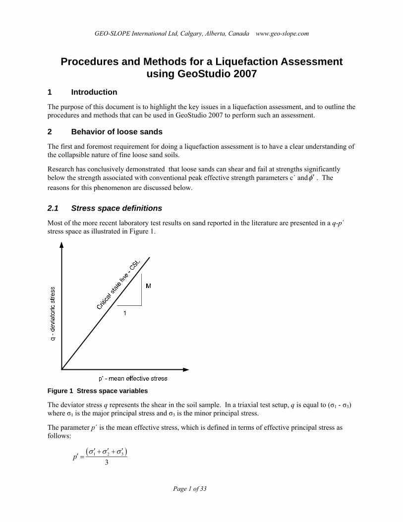
Consider an undrained triaxial test on a loose sand sample consolidated to the isotropic stress state represented by Point A in Figure 2. Upon loading the effective stress path follows a curved path with rising deviator stress until the maximum deviator stress – referred to as the collapse point – is encountered. At that point there is a sudden tendency for volumetric compression, that is, collapse, which is offset by a rapid and large increase in the pore water pressures. The rapid rise in pore pressures leads to a decrease in mean effective stress and deviator stress. The rapid decrease in the deviator stress, which can be viewed as a loss of strength, is termed liquefaction. The strength path eventually intersects the CSL, at which point the mean effective stress, deviator stress, and void ratio remain constant with further shearing.

q

p'A

Collapse point

Steady-statestrength

Figure 2 Effective stress path for loose sand in an undrained triaxial test

If a series of undrained triaxial tests are completed on a series of samples at the same initial void ratio the stress paths will appear as illustrated in Figure 3. A straight line can be drawn from the steady-state strength through the peaks or collapse points. Sladen, D’Hollander and Krahn (1985a) called this line a Collapse Surface.


Page 3 of 33

q

p'


Collapse surface

Figure 3 Collapse surface illustration

Some researchers have proposed that the collapse surface line should pass through the origin of the plot (e.g., Vaid and Chern (1983). Since flow liquefaction cannot occur below the steady-state point, the authors crop the lower end of the collapse line as illustrated in Figure 4.

Figure 4 Definition of Flow Liquefaction Surface (FLS)

As noted, a soil can liquefy when the stress path reaches the collapse surface during undrained loading; consequently, Kramer (1996, p. 363) named the collapse surface a flow liquefaction surface (FSL). As discussed subsequently, other research has demonstrated that loose sands can also collapse under drained loading; however, once collapse is initiated the soil can either: a) liquefy and follow a similar stress path as shown in Figure 2 if drainage is impeded; or b) undergo volumetric compression if drainage is permitted, allowing the stress path to proceed more steadily towards the CSL. Research has shown that collapse can be initiated during drained loading for both dry and saturated soils. The FSL designation is consequently too narrow because a soil can collapse without ‘flowing’ (that is, liquefying). The collapse surface designation is more general.

The undrained steady-state strength of loose sand tends to be a relatively small value. Consequently, the difference between whether the collapse surface is projected through the origin or through the steady-state point on the CSL is relatively small. For practical purposes and the interpretation of field behavior the two approaches are in essence the same.


Page 4 of 33

Chu et al. (2003) called the collapse line an Instability Line (IL). The reasons for this choice of nomenclature is rather perplexing considering that the collapse phenomenon had been adequately described by previous researches. Nonetheless, the instability line is essentially equivalent to the FLS and the collapse line.

The more general collapse surface designation and a line that passes through the steady-state point on the CSL are used here and in GeoStudio.

Drained conditions

Sasitharan et al. (1993) at the University of Alberta were able to clearly demonstrate that the sand grain-structure can collapse during fully drained loading as well as during undrained loading. Collapse can occur at a mobilized friction angle m that is well below the conventional effective friction angle .

The fact that collapse of a loose sand grain-structure can be initiated during fully drained loading is critical to understanding the stability of the sand slopes. The initiation of collapse during drained loading can result in: a) an undrained liquefaction type response resulting in rapid loss of strength (described previously); or b) a drained response that is characterized by a decrease in the void ratio (that is, collapse). It is tempting to conclude that scenario (b) would improve the stability of a slope because the decrease in void ratio leads to a more stable grain-structure. This, however, is not necessarily the case because collapse in one region of a slope would cause the redistribution of stresses to other regions of the slope. This would in turn promote a slope failure.

Dry sand

Skopek et al. (1994) at the University of Alberta demonstrated that collapse of a loose sand grain-structure can even occur in dry sand (Figure 5 and Figure 6). The soil specimens were loaded by decreasing the mean effective stress at a constant deviator stress.

Of great significance is the associated change in volume or void ratio. Initially, the void ratio remained relatively constant while the mean effective stress diminished (Figure 6), but then the void ratio suddenly decreased dramatically, particularly for the very loose sample. The sudden decrease in void ratio reflects the collapse in the grain-structure. After the collapse, the void ratio continues to decrease with a further reduction in the mean effective stress. This continues until the stress state reaches the CSL.

The tendency for volume change would have resulted in a dramatic and sudden increase in the pore pressures had the specimen been initially saturated and the drainage valve closed at the point of collapse. Such a condition would have triggered liquefaction.


Page 5 of 33

0

50

100

150

200

250

300

0 50 100 150 200 250 300

Effective normal stress p'(kPa)

Sh

ea

r st

ress

q (

kP

a )

Loose

Very loose

Steady State Line

Figure 5 Tests on dry sand (after Gu and Krahn, 2002)

0.72

0.74

0.76

0.78

0.80

0.82

0.84

0.86

0.88

0.90

0 50 100 150 200 250 300

Effective normal stress ( kPa )

Vo

id r

atio

e

Very loose

Loose

Collapse point

Steady State Line

Figure 6 Tests on dry sand (after Gu and Krahn, 2002)

Cyclic or dynamic loading

The above discussion on collapse behavior has considered only monotonic (static) loading. Cyclic loading can also lead to liquefaction, as is illustrated in Figure 7. Consider a soil at Point B subject to a cyclic load. The cyclic loading causes a continuous increase in the pore pressures (and therefore decrease in mean effective stress) until the cyclic stress path intersects the collapse surface. Under saturated undrained conditions the sand can then liquefy and the strength will suddenly fall along the collapse surface to the steady-state point.


Page 6 of 33

q

p'

B

Collapse surface


Figure 7 Cyclic stress path from B to the collapse surface

State boundary surface

Incidentally, the straight-line collapse surface defined by Sladen et al. (1985) is actually a simplification of the actual shape. Sasitharan et al. (1993) demonstrate that the collapse surface is actually curved to form a true state boundary surface. For practical purposes, however, the straight line approximation is more than adequate, particularly given the uncertainty associated with measuring or estimating the collapse surface parameters.

2.3 Required stress path

Sasitharan et al. (1993) have argued that a stress path must attempt to cross the collapse surface for the sand-grain structure to collapse (Figure 8). The stress state must therefore be on or below the collapse surface at the initiation of loading. The shortest stress path shown in Figure 8 that intersects the collapse surface is generated by decreasing the mean effective stress while maintaining constant deviator stress. Such a stress path is very similar to the path followed when an unsaturated slope becomes partially submerged. The rising water levels and associated loss of soil suction can therefore be trigger mechanism for slope instability.

In the strictest sense, a stress state cannot exist above the current collapse surface. As explained in the next section, the collapse surface can be ‘dragged open’ (that is, the collapse line is ‘dragged’ to a higher position or steeper inclination) under certain loading conditions. Such loading conditions are associated with a decrease in void ratio or with densification.


Page 7 of 33

Figure 8 Illustrative stress paths from X to collapse surface for grain-structure collapse

2.4 Collapse surface parameters

The two parameters required to define the collapse surface in q-p’ stress space are the angle of inclination of the collapse surface ML and its intersection qss with the critical state line (the subscript L stands for ‘liquefy’). The parameter qss represents the steady-state strength and is approximately equal to 2 x Css, where Css is the intersection of the collapse line with the Mohr-Coulomb failure line in : stress space. (Note: this is only strictly valid for triaxial loading conditions; however, the approximation is reasonable for the purpose of field analyses). The slope ML is related to the friction angle L by the relationship:

6sin

3 sinL

LL

Collapse surface angles

The collapse surface inclination generally increases as the initial density increases. The lowest L values

correspond with very loose sand. As the density increases the inclination increases and may approach the critical state line when the sand reaches a medium density. Chu et al. (2003) show collapse line slopes greater than the CSL for dense sands but this issue will not be addressed in this report.

Figure 9 is a graph published by Chu et al. (2003). The inclinations L vary between 18.3 and 34.5

degrees (ML is between 0. 7 and 1.4). The corresponding void ratios vary between 0.972 and 0.864.


Page 8 of 33

Figure 9 Collapse line inclination as a function of density (after Chu, et al. 2003)

Sladen et al. (1985a) presented the data for three different isotropically consolidated sands as shown in Table 1. The lowest L is 14.3 degrees and the highest is 18.5 degrees.

Table 1 Table of data showing measured collapse line inclinations (after Sladen et al. 1985b)

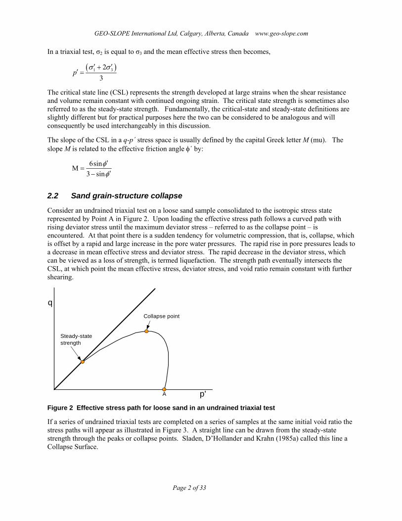
Lade (1993) presented a summary of L values as shown in Figure 10. Despite the scatter, there is clear

evidence for the trend of increasing L with increasing density. For relative densities less than 50 percent

the range is about 15 to 25 degrees.


Page 9 of 33

Figure 10 Range of L for variation of initial relative density (Lade, 1993).

Kramer (1996, p. 364) makes this statement in his text book: for ‘isotropic initial conditions, the slope of the FLS ( L ) is often about two-thirds the slope of the drained failure envelope for clean sand.’ These

data can be used as a guide for selecting L values.

Steady-state strengths

The steady-state strengths of loose sand tend to be relatively small. Sladen et al. (1985b) were of the view that the undrained steady-state strengths at the Nerlerk Berm failures in the Beaufort Sea were less than about 2 kPa. This was based on back analyses of the failures and the eventual very flat slopes of the sliding mass.

The data presented in Figure 9, also suggests that the steady-state strength for loose clean sands is very low as the curves tend to converge near the origin of the graph.

Castro el al. (1992), as part of a re-evaluation of the liquefaction failure that occurred at the Lower San Fernando Dam in 1971, concluded that the undrained steady-state strength for the hydraulic fill in the dam was likely in the range of 20 to 30 kPa. This relatively high value is likely reflective of the significant fines content in the hydraulic fill.

The published information on the steady-state strength is rather meager and not sufficient to select a value for stability analyses with any confidence. Fortunately, stability analyses are not all that sensitive to the steady-state strength parameter. The analyses are much more sensitive to the inclination of the collapse surface, which can be estimated more accurately.

Effect of fines content

The amount of fines (silt and clay) in the sand can have a significant effect on the potential liquefaction of the sand. Sladen et al. (1985b) concluded: “the potential for liquefaction is much lower for clean sand


Page 10 of 33

than for dirty sand, all else being equal”. They go on to state: “a high fines content will also reduce permeability and increase compressibility making an undrained response to any given loading condition more likely”.

More recently, Seid-Karbasi and Byrne (2007) have investigated the effect of silty-clayey layers on the liquefaction behavior of sands. They have shown that these types of layers can act as barrier to the dissipation of excess pore-pressure associated with the collapse of the sand grain structure and thereby contribute to the potential instability. The inference is that in the absence of such impeding layers the excess pore pressure could likely dissipate faster and the sand would fail more in a drained manner than in an undrained manner. The outwash sand can be stratified with layers of varying fines content. This stratification can played an important role in the behavior of the sand and the resulting stability of earth structures.

2.5 Case histories

The concept of a collapsible sand grain-structure has provided the basis for a rational explanation for the failure of various earth structures. The following sections briefly highlight the key aspects of three case histories.

Nerlerk Berm

In the early 1980’s artificial sand islands were constructed in the Beaufort Sea to facilitate hydrocarbon exploration. Construction of the Nerlerk berm started in 1982 at a location where the sea depth was about 45 m. The berm was initially constructed by dumping sand from barges. More sand was later added on the berm via hydraulic methods. The sand was dredged from the seabed and pumped through a floating pipeline.

The sand placement caused at least five side-slope failures as illustrated in Figure 11. Subsequent studies by Sladen et al. (1985a, 1985b) provided the collapse surface rational for the slope failures. Ultimately, it was concluded that the failures were the result of liquefaction in the sand due to the static loading resulting from the hydraulically placed sand.


Page 11 of 33

Figure 11 Beaufort Sea Nerlerk Berm liquefaction slope failures (after Sladen et al. 1985b)

Hill-side mine waste dumps

There have been numerous hill-side waste dump slope failures at open-pit coal mining operations in the Canadian Rocky Mountains, some with very large run-out distances (Dawson et al. 1998). The following two figures (Figure 12 and Figure 13) illustrate the Cougar 7 dump failure at the Greenhills Mine located near Elkford, British Columbia. Of significance is the very long run-out distance relative to the dump size.

Dawson et al (1998) did an extensive study of these dump failures and came to the conclusion that the dumping process created layers of fine sediments at the base of the dump and/or within the dump. These fine layers became saturated due to hill-side seepage or infiltration. The subsequent dumping caused further static loading of these fine-sediment layers, which in turn caused the grain-structure to collapse. Furthermore, the authors demonstrate that the strength mobilized in the fine-grained layers at the point of collapse was significantly less than the peak c´ and strength parameters. The large run-out distances are attributed to the excess pore-pressures that developed subsequent to the grain-structure collapse.


Page 12 of 33

Figure 12 Profile of the Cougar 7 dump failure at the Greenhills Mine (after Dawson et al, 1998)

Figure 13 Plan view of run-out at the Cougar 7 dump failure at the Greenhills Mine (after Dawson et al 1998)

Coal stockpiles

Dramatic flow-like slope failures have occurred in stockpiles of coking coal at a north Australian coal export terminal. Some of the slips have flowed up to 60 m beyond the original stockpile toe when the dumps where 10 to 14 m high (Eckersley, 1990). The failures occurred after the coal became saturated (or nearly saturated) due to heavy rainfall. Eckersley (1990) also concluded that the failures were initiated under essentially static drained conditions at a mobilized strength much less than what would be represented by conventional peak effective stress strength parameters c´ and . The resulting initial movements lead to the rapid generation of excess pore-pressures and the accompanying strength loss that


Page 13 of 33

caused the sudden acceleration of the sliding mass. Eckersley’s explanation of why the failures occurred is entirely consistent with the concepts associated with a sand grain-structure collapse.

2.6 Commentary and summary

The fact that loose sands can have a collapsible grain-structure has now been well established. It is not only a laboratory observed phenomena but supported by observed field behavior.

When the grain-structure collapses, the mobilized shear strength can be well below the conventional peak effective strength parameters c´ and .

Under undrained conditions, the pore-pressures can rise sharply at the point of collapse and the strength fall down suddenly to low undrained steady state strength. This sudden rise in pore-pressure and associated strength loss can manifest itself in liquefaction.

The concept of a collapse surface is a highly useful tool for assessing the liquefaction potential of earth structures.

3 Stress state regions

When interrupting the results of a GeoStudio analysis it can be useful to think of the q-p´ space in terms of regions. It helps to understand why certain elements are marked as liquefiable and others are not.

3.1 Liquefiable region

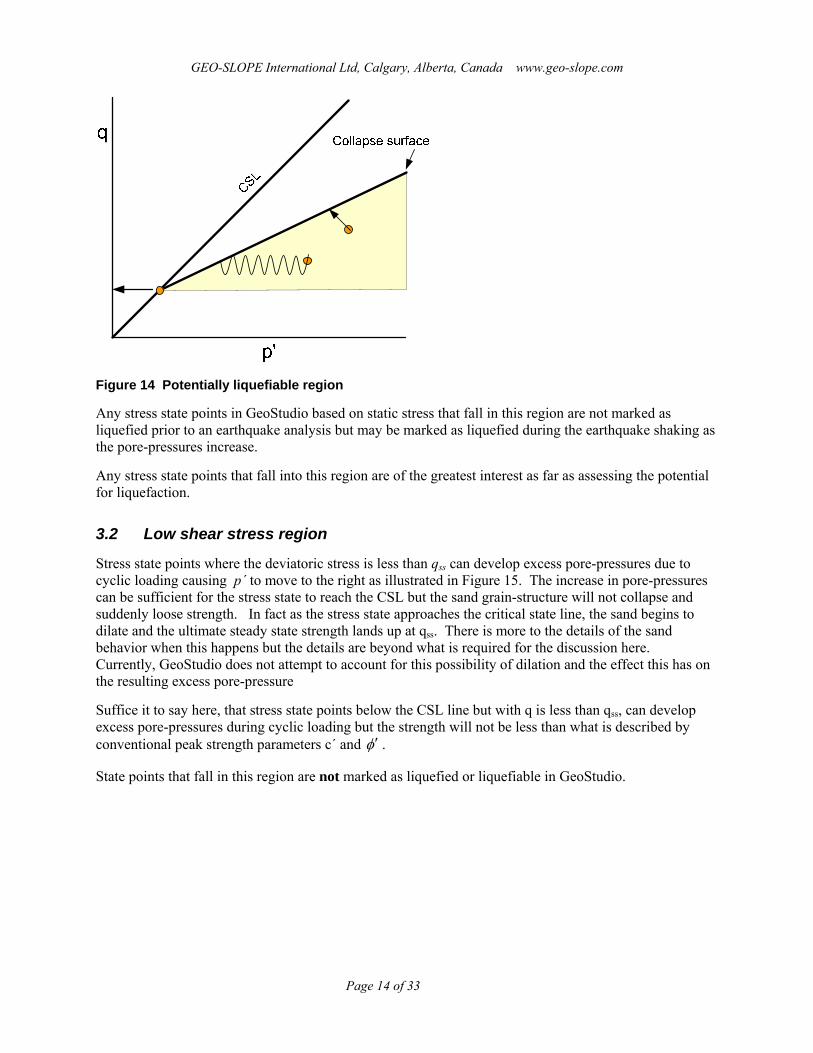
The shaded region in Figure 14 is the region where the sand grain structure can collapse and under undrained condition the strength can suddenly fall down to the steady-state strength.

Any stress state with a q-p´ ratio in this region could potential move onto collapse surface and potentially liquefy. Any increase in pore-pressure, from earthquake shaking for example, would cause p´ to diminish and the stress state point could move to the left unto the collapse surface. Additional external static loading could also cause the shear stress (q) to increase and thereby move onto the collapse surface.


Page 14 of 33

Figure 14 Potentially liquefiable region

Any stress state points in GeoStudio based on static stress that fall in this region are not marked as liquefied prior to an earthquake analysis but may be marked as liquefied during the earthquake shaking as the pore-pressures increase.

Any stress state points that fall into this region are of the greatest interest as far as assessing the potential for liquefaction.

3.2 Low shear stress region

Stress state points where the deviatoric stress is less than qss can develop excess pore-pressures due to cyclic loading causing p´ to move to the right as illustrated in Figure 15. The increase in pore-pressures can be sufficient for the stress state to reach the CSL but the sand grain-structure will not collapse and suddenly loose strength. In fact as the stress state approaches the critical state line, the sand begins to dilate and the ultimate steady state strength lands up at qss. There is more to the details of the sand behavior when this happens but the details are beyond what is required for the discussion here. Currently, GeoStudio does not attempt to account for this possibility of dilation and the effect this has on the resulting excess pore-pressure

Suffice it to say here, that stress state points below the CSL line but with q is less than qss, can develop excess pore-pressures during cyclic loading but the strength will not be less than what is described by conventional peak strength parameters c´ and .

State points that fall in this region are not marked as liquefied or liquefiable in GeoStudio.


Page 15 of 33

Figure 15 Stress states where q is less than qss

3.3 Region between CSL and collapse surface

Conceptually, stress state points cannot exist in the region between the collapse surface and the steady-state line. Or stated another way, stress state points cannot exist above the collapse surface. If there was a tendency for a stress path to cause the stress state point to move above to the collapse surface, the sand-grain structure would either collapse or possibly the sand would densify and the collapse surface would shift upwards with the stress state point as already discussed in Section 2.3 above.

Figure 16 Region where elements are marked as liquefied

Numerically, in a GeoStudio analysis a stress state point can exist above the collapse surface. This is results from an inaccurate description of the stress - distribution or collapse surface definition. Practically what it means is that the soil is in a very precarious unstable state and that any amount of static or dynamic disturbance could cause the sand grain-structure to collapse.


Page 16 of 33

In GeoStudio any computed stress state points that fall into this zone are marked as liquefied and no excess pore-pressures are allowed to develop.

3.4 Stress state points above the CSL

Of course in reality no stress state points can exist above the CSL – the shear stress cannot be greater than the shear strength. Again, numerical in a GeoStudio analysis it is possible to compute stresses that fall above the CSL line. What this means is that the computed stress distribution is not perfect.

Elements with a stress state that fall above the CSL are not marked as liquefied or liquefiable. Practically, the field shears stress is at the peak shear strength and for analysis purposes the soil is assign the conventional peak strength parameters c´ and . Also no excess pore-pressure is allowed to develop.

4 Effect of initial static shear and confining stress

The confining stress and shear stress that exist in the ground prior have a major influence on the liquefaction potential.

Consider Points A and B in Figure 17. Let’s assume the shear stress is the same at both points. Point A being at a lower confining stress (low p´) is very close to the collapse surface and any amount of strong motion shaking could cause the stress state to move onto the collapse surface and suddenly fall down to the steady-state strength. Point B on the other hand is at a much higher confining stress (higher p´) and therefore a very significant amount of excess pore-pressure would need to develop during the shaking for the stress state to reach the collapse surface.

Figure 17 Effect of confining stress on the liquefaction potential

Now consider Points A and B at different initial shear stresses but at the same confining stress as illustrated in Figure 18. Point A is again very close to the collapse surface and any amount of shaking disturbance could cause liquefaction. Whereas Point B is a long way away from the collapse surface and high excess pore-pressures would need to develop during earthquake shaking for liquefaction to occur.


Page 17 of 33

Figure 18 Effect of initial static shear stress on the liquefaction potential

This illustrates why the initial static stress conditions are so critical to assessing the liquefaction potential.

Researchers that have used a cyclic stress approach to assessing the potential for liquefaction early on recognized the strong influence of the initial static confining stress and initial static shear stress. From this evolved what are known as Confining Stress (Ks) and Shear Stress (Ka) correction factors. Such correction factors are not required in the context of a collapse surface.

More details on these correction factors are given in the QUAKE/W Engineering Book on pages 99 to 104.

The beauty about the collapse surface concept is that it inherently accounts for the initial shear and confining stresses as illustrated above. No correction factors are required as in the cyclic stress approach.


Page 18 of 33

5 Initial insitu stress conditions

Now let’s look at the influence of the initial insitu static stress condition and how to use GeoStudio to examine this. We will start with a simple 1D column illustrated in Figure 19, which is adequate for representing horizontal ground surface conditions.

Ele

vatio

n -

m

0

2

4

6

8

10

12

14

16

18

20

Figure 19 One dimensional column representing horizontal ground

The water table is at the ground surface. The total unit weight of the soil is 20 kN/m^3 and the unit weight of the water is taken to be 10 kN/m^3 for convenient discussion purposes.

The convention effective strength parameters c´ and φ´ are zero and 30 degrees.

To begin with we’ll set Ko to 0.5.

The steady-state shear strength is set to 5 kPa; this makes qss = to 10 kPa.

Also, to start with we’ll make the collapse surface inclination 18 degrees.

Now we can do an Insitu type of analysis in SIGMA/W. It is necessary to select the Elastic-Plastic Material Model for this analysis. The specified material properties are shown in the following screen capture.


Page 19 of 33

The SIGMA/W Insitu results indicate that the lower 14 m of the soil column is liquefied or in a liquefiable state as shown in Figure 20.

Ele

vatio

n -

m

0

2

4

6

8

10

12

14

16

18

20

Figure 20 Liquefaction zone with Ko equal to 0.5


Page 20 of 33

The reason for this is that the q/p´ ratio is above or very close to the specified collapse surface. This can be vividly illustrated by taking the q and p´ stress profiles into EXCEL and plot these values relative to the CSL and the position of the collapse surface. The end result is shown in Figure 21. At low stress levels the field q/p´ ratio is just below the collapse surface and at higher stress levels the q/p´ ratio is just above collapse surface and consequently the liquefaction shading in Figure 20.

0

20

40

60

80

100

120

140

160

180

200

0 20 40 60 80 100 120 140 160 180 200

Deviatoric Stress ‐q

Mean effective stress ‐ p'

CSL Collapse surafce Field q/p' ratio

Figure 21 Field q/p´ ratios relative to the collapse surface with Ko equal to 0.5

If this was indeed representative of the actual field conditions, there would be little or no value doing a QUAKE/W dynamic earthquake analysis. The simply SIGMA/W Insitu analysis implies that any amount of strong motion shaking could in all likelyhood cause the soil to liquefy.

The situations for Ko equal to 0.6, 0.8 and 0.95 are shown in the following graphs.

When Ko is 0.6, some strong ground motion may result in sufficient generation of excess pore-pressure for a significant portion of the column to liquefy. If Ko is 0.8 the field q/p´ is fairly far away from the collapse surface and it would mean that large excess pore-pressures would need to develop for liquefaction to occur. If Ko were to be 0.95, large excess pore-pressures might develop but liquefaction would be highly unlikely.

The SIGMA/W Insitu analyses indicate no liquefaction shading when Ko is greater than 0.6. This is because the field q/p´ ratios are not on or above the collapse surface.


Page 21 of 33

0

20

40

60

80

100

120

140

160

180

200

0 20 40 60 80 100 120 140 160 180 200





0

20

40

60

80

100

120

140

160

180

200

0 20 40 60 80 100 120 140 160 180 200






Page 22 of 33

0

20

40

60

80

100

120

140

160

180

200

0 20 40 60 80 100 120 140 160 180 200





From these simply SIGMA Insitu analyses we can readily see how strongly the potential for liquefaction is influenced by the initial static insitu stress state conditions.

From these analyses we can see that potential for liquefaction is heavily influenced by the shear stresses that exist in the ground prior to any earthquake shaking.

A simple preliminary SIGMA/W analysis can also help with understanding the generation of liquefaction zones in a later QAUKE/W analysis. If the field q/p´ ratios are close to the collapse surface then liquefactions zones will develop very quickly in a QUAKE/W analysis where as if the static field q/p´ ratios are far removed from the collapse surface the QUAKE/W analysis may not show any liquefaction zones at the end of the earthquake shaking. This is discussed further below.


Page 23 of 33

6 Two-dimensional situation

Now let’s look at the following simple 2D case. It is assumed that the foundation material is loose and potentially liquefiable. The dam embankment material is assigned the same material properties as the foundation except that it is not deemed to be liquefiable; that is, no collapse properties are assigned to the dam.

Underdrain

Distance - m

0 5 10 15 20 25 30 35 40 45

Ele

vatio

n -

m

0

2

4

6

8

10

12

14

Figure 25 Illustrative 2D case

Both materials are assigned an effective friction angle φ´ equal to 30 degrees with c´ equal to zero. This makes the slope of the CSL equal to 1.2.

For illustrative purposes, the foundation is assigned collapse surface properties. The inclination is 18 degrees. The steady-state strength is set to zero. This is an unrealistic field value but it is useful for illustration purposes. By making Css zero, the q/p´ ratio is a constant making it easier to compare the liquefiable shaded areas with q/p´ contours. For 18 degrees the slope of the collapse surface in q - p´ space is 0.69.

The following figure shows the CSL and collapse surface with these parameters. Any q/p´ ratios that fall between the two lines will be marked as liquefiable.

0

20

40

60

80

100

120

140

160

180

200

0 20 40 60 80 100 120 140 160 180 200



CSL Collapse surafce

Figure 26 Position of CSL and collapse surface


Page 24 of 33

We can do a SIGMA/W Insitu type of analysis to look at the situation under static insitu loading conditions. The pore-pressure conditions will come from the Water Table definition. To obtain the information of interest, it is necessary to use Effective-Drained Parameters with an Elastic-Plastic constitutive model.

6.1 Ko equal to 0.5

The following Figure 27 shows the results when Poisson’s ratio is 0.3334 which represents a Ko of 0.5. The shaded area is where the q/p´ ratio is between the CSL and the collapse surface. Shown as well are q/p´ contours. Recall that the slopes of the two lines are 1.2 and 0.69, consequently the shaded area falls between the 1.2-contour and the 0.7-contour.

0.7 1

1.2

Underdrain

Distance - m

0 5 10 15 20 25 30 35 40 45

Ele

vatio

n -

m

0

2

4

6

8

10

12

14

Figure 27 Liquefiable zone and q/p’ contours with Ko equal to 0.5

6.2 Ko equal to 0.667

Now if we set Ko to 0.667 (Poisson’s ratio = 0.4) the situation is as follows. The potentially liquefiable zone has now shifted and shrunk because of a different insitu static stress distribution.

0.7

1

1.2

Underdrain

Distance - m

0 5 10 15 20 25 30 35 40 45

Ele

vatio

n -

m

0

2

4

6

8

10

12

14



Page 25 of 33

6.3 Ko equal to 0.818

Setting Poisson’s ratio to 0.45 and making Ko 0.818 results in the following situation. Again the potentially liquefiable area has shifted and become smaller.

0.7

1

1.2

Underdrain

Distance - m

0 5 10 15 20 25 30 35 40 45

Ele

vatio

n -

m

0

2

4

6

8

10

12

14


6.4 Effect of insitu static stresses

Again as was demonstrated earlier for the 1D analysis, the above figures demonstrate the strong influence that the static insitu stresses have on the potential for liquefaction.

6.5 Stability based on static stresses

At this stage it is possible to do a stability analysis with SLOPE/W to look at the situation if indeed the strength in the liquefiable zone should fall to the specified steady state strength.

The following diagram shows a potentially liquefiable zone when Css is 5 kPa and Ko is 0.667.

Underdrain

Distance - m

0 5 10 15 20 25 30 35 40 45

Ele

vatio

n -

m

0

2

4

6

8

10

12

14

Figure 30 Liquefiable zone with Ko equal to 0.5 and Css equal to 5 kPa

Let us now make the assumption that the strength in the shaded area has fallen down to the undrained steady-state strength for some undefined reason. We need to define a new material for the stability


Page 26 of 33

analysis. The new foundation material will have all the properties as before except the collapse surface angle will be set to zero. This means that when the slip surface is in the shaded area the strength will be 5 kPa.

Consider the slip surface in the following figure. The cohesive and frictional strength along the slip surface are shown in figure. Notice how in the middle portion of the slip surface the frictional strength is zero and the cohesive strength is 5 kPa which represents the Css strength.

(Unfortunately, currently it is not possible to show the shaded liquefiable zone in SLOPE/W – watch for this in a future version).

Underdrain

Distance - m

0 5 10 15 20 25 30 35 40 45

Ele

vatio

n -

m

0

2

4

6

8

10

12

14

Figure 31 Stability with reduced strength in the liquefiable area

Cohesion :Cohesive

Friction :Frictional

kPa

X (m)

-5

0

5

10

15

20

25

10 12 14 16 18 20 22 24 26

Figure 32 Cohesive and frictional strength along the slip surface


Page 27 of 33

Often it is necessary to create a new material for the stability analysis if the objective is to look at the Css strength alone; that is, use the Css strength but make the collapse surface inclination zero.

It is important to note at this stage that much can be done in the liquefaction evaluation process without using QUAKE/W. Adding a QUAKE/W analysis is necessary only in the later stages of the evaluation process, if at all. Sometimes, a definitive conclusion can be reached before even proceeding onto a dynamic shaking analysis with QUAKE/W. If, for example, the margin of safety is already less than 1.0 under static conditions, then there is likely no value in doing a QUAKE/W analysis.

7 Case history

Now let’s look at the above discussion in the context of a case history. We can do this by abstracting information from the QUAKE/W Detailed Example called the Upper San Fernando Dam.

7.1 Development of liquefiable zone during the earthquake shaking

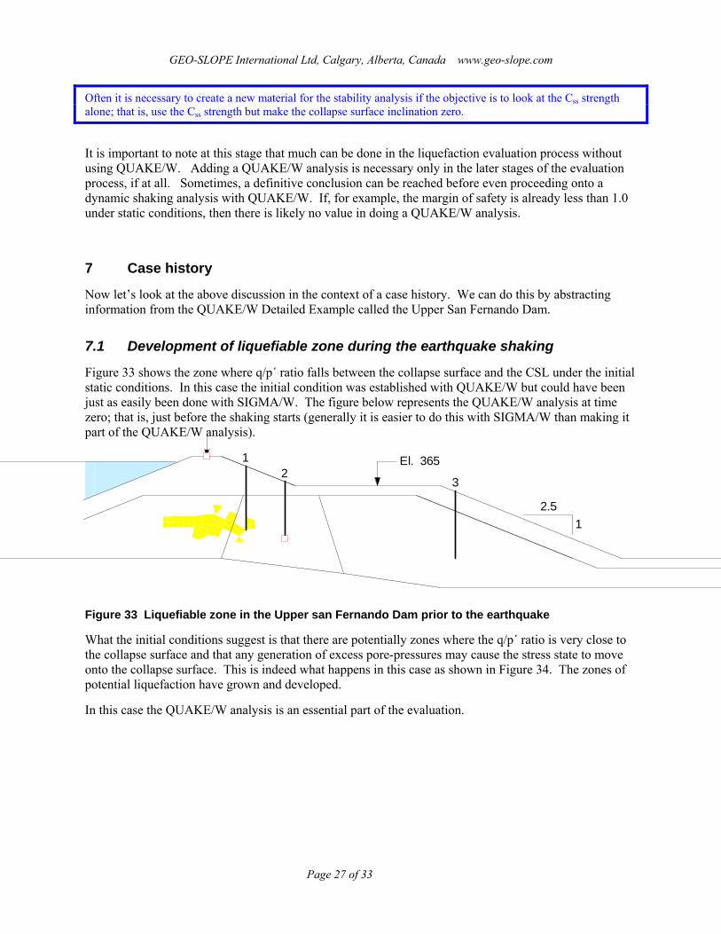
Figure 33 shows the zone where q/p´ ratio falls between the collapse surface and the CSL under the initial static conditions. In this case the initial condition was established with QUAKE/W but could have been just as easily been done with SIGMA/W. The figure below represents the QUAKE/W analysis at time zero; that is, just before the shaking starts (generally it is easier to do this with SIGMA/W than making it part of the QUAKE/W analysis).

12

3

El. 365

1

2.5

Figure 33 Liquefiable zone in the Upper san Fernando Dam prior to the earthquake

What the initial conditions suggest is that there are potentially zones where the q/p´ ratio is very close to the collapse surface and that any generation of excess pore-pressures may cause the stress state to move onto the collapse surface. This is indeed what happens in this case as shown in Figure 34. The zones of potential liquefaction have grown and developed.

In this case the QUAKE/W analysis is an essential part of the evaluation.


Page 28 of 33

12

3

El. 365

1

2.5

Figure 34 Liquefiable zones in the Upper San Fernando Dam after the earthquake

You will notice in this Detailed Example, that special materials have been created for the post-earthquake analyses so that the liquefied zones have just the steady-state strength Css .

7.2 Post-earthquake permanent deformation

As presented in the Detailed Example documentation, it is possible to evaluate the post-earthquake deformation using a SIGMA/W Stress Redistribution type of analysis. This can be done based on static stresses or by including the dynamic inertial forces.

Using static stresses

There is field evidence indicating that sometimes the most significant deformations occur after the shaking has stop. At the Lower San Fernando Dam, for example, it is believed that the upstream failure occurred immediately after the earthquake strong motion had stop. The thinking is that the dynamic inertial stress had disappeared by the time the failure or large deformations occur due to the associate strength loss.

The same logic is used in the post-earthquake analysis of the Upper San Fernando Dam.

When this is the objective it is important to indentify the initial static stresses in the Stress Redistribution analysis. Using the stresses at the end of the shaking may numerically still include some residual dynamic stresses which is not desirable. This can be avoided by selecting the initial static stress as highlighted in the following dialog box in SIGMA/W. Note the selection of Time:(initial) for the stresses conditions and Time:(last) for the PWP conditions. We want to use the pore-pressure conditions at the end of the shaking but use the initial static stress conditions.


Page 29 of 33

Including the dynamic inertial forces

It is also possible to include the earthquake induced inertial forces in the permanent deformation analysis. This is done with a SIGMA/W Dynamic Deformation type of analysis. With this type of analysis SIGMA automatically does a stress redistribution analysis at each saved time step. If QUAKE/W, for example saved the results for 100 times steps, SIGMA/W would do 100 stress redistribution analyses.

The selections in the KeyIn Analysis dialog box in this case would be as shown below. There is no option as to which stress condition is used. The static plus dynamic stresses are automatically used at each time step.

The starting pore-pressures come from the initial conditions. The increasing pore-pressures are used at each time step as they develop.

The reduced strengths for the liquefiable zones are also used as they develop during the shaking.


Page 30 of 33

8 QUAKE/W analysis

It is very important to use only the strong motion portion of an earthquake time history record in the QUAKE/W analysis step in a liquefaction evaluation. Including the early small trembling motion at the start and the end of record makes the QUAKE/W analysis unnecessarily difficult (and even frustrating sometimes). The computing time takes too long and it creates too much data making the viewing of results too slow.

Remember, it is only the large dynamic shear stresses that cause the generation of excess pore-pressures and this happens only during the most intense motion.

This is discussed on Pages 155 and 156 in the QUAKE/W Engineering Book.

The record shown in Figure 35 has a duration of almost 50 sec and includes over 12,000 data points. This record could be easily reduced to the one in Figure 36 for a QUAKE/W liquefaction-assessment studying. The modified record is only about 18 sec with about 5000 data points. The record could be further modified by deleting every other data point without having a noticeable effect on the QUAKE/W results.

Modifying the earthquake record is often the most conveniently done in a spreadsheet (EXCEL). Once the data has been imported into QUAKE/W, all the data can be selected and copied into EXCEL for modification (right mouse click in the list box of the data). Once the record has been modified, you can paste the data back into QUAKE/W through the clipboard.

The modification can also be done directly in QUAKE/W by group selection of certain portions of the data points and clicking on delete.

Acc

ele

ratio

n (

g )

Time (sec)

-0.2

-0.4

-0.6

-0.8

0

0.2

0.4

0.6

0 10 20 30 40 50

Figure 35 Raw time history record


Page 31 of 33

Acc

ele

ratio

n (

g )

Time (sec)

-0.2

-0.4

-0.6

-0.8

0

0.2

0.4

0.6

0 5 10 15 20

Figure 36 Modifies time history record

The first step is to remove the low trembling noise at the ends of the record and then consider removing every other data point, for example, if the data was recorded at a very small time interval.

Remember, when in doubt you should do most of your preliminary work with a simplified analysis and then near the end of the modeling try some more complicated analyses to determine if it makes a significant difference to your conclusions.

9 Field Ko conditions

Earlier it was been demonstrated that the potential for liquefaction is highly dependent on the static insitu stress state. This then begs the question, what is an appropriate Ko.

Generally, liquefaction is associated with loose fine sands. For a sand to be in a loose state in the field it likely was deposited in a calm fluvial or sedimentation environment and has not been subject to past loading and unloading. In a sense, it is like the material is normally consolidated.

For normally, consolidated soils Ko can be estimated from the relationship:

1 sinoK

Looking at it another way, it is unlikely that loose liquefiable sands have a high Ko. If the sand has a high Ko it is likely no longer in a loose state because the past loading and unloading that caused Ko to be high also densified the soil.

These are general comments intended to start the GeoStudio user’s thought process on this issue. Clearly, this is an important issue and needs to be assessed carefully in the context of project specific conditions.


Page 32 of 33

10 Commentary and recommendations

The purpose here has been to provide GeoStudio Users with a guideline for doing a liquefaction assessment. In summary, to use GeoStudio effectively for a liquefaction assessment the following is essential.

First and foremost, it is essential to have a clear understanding of the collapsible grain-structure of loose fine sands. That the grain-structure can collapse and that the strength can suddenly fall down to the undrained steady-state strength has been conclusively demonstrated by laboratory tests and field observation.

The user must have an understanding of how GeoStudio flags elements as potentially liquefiable in the context of regions in q-p´ stress space.

Recognize that the definition of a collapse surface automatically accounts (corrects) for the shear and confining stress in the ground. No other correction factors are required like those used in the cyclic stress approach.

Accept that fact that the liquefaction potential is tightly tied to the insitu static stress state.

Use SIGMA/W, and maybe SLOPE/W, to assess the situation before moving unto a QUAKE/W analysis. A QUAKE/W analysis should only be undertaken after an initial assessment based on static stresses. Starting with a complicated QUAKE/W analysis should be avoided.

When a QUAKE/W analysis is undertaken, only the strong motion portion of a time history record should be used.

To be clear that QUAKE/W alone cannot provide any information about permanent deformations. QUAKE/W can only provide information about the dynamic inertial forces and the resulting associated generation of excess pore-pressures.

Understand that permanent deformations can only be estimated by doing a SIGMA/W Stress Redistribution type of analysis or a SIGMA/W Dynamic Deformation type of analysis.

Before doing a permanent deformation analysis, it is important to first check the stability using the post-earthquake pore-pressures and reduced strengths resulting from collapse of the sand-grain structure. If the stability analysis shows the structure to be unstable at this stage (factor of safety close to or less than 1.0) then there is little value in a permanent deformation analysis – the structure has already failed and collapsed. If such an analysis is done it may provide a picture of the post-failure displacement field, as in the Lower San Fernando Dam case history, but the magnitudes of the computed displacements will be meaningless. In short, GeoStudio cannot be used for a post-failure deformation analysis.

Prepared by:

Dr. John Krahn


Page 33 of 33

11 References

Arya, L.M. and Paris, J.F. (1981). A physioempirical model to predict the soil moisture characteristic from particle-size distribution and bulk density data. Soil Science Society of America Journal, 45: 1023-1030.

Castro, G., Seed, R.B., Keller, T.O. and Seed, H.B. (1992). Steady-state strength analysis of Lower San Fernando dam slide, ASCE Journal of Geotechnical Engineering, Vol. 118, pp 406-427.

Chu, J., Leroueil, S. and Leong, W.K. (2003). Unstable behavior of sand and its implication for slope stability, Canadian Geotechnical Journal, Vol. 40, pp 873-885.

Dawson, R.F., Morgenstern, N.R. and Stokes, A.W. (1998. Liquefaction flow slides in Rocky Mountain coal mine waste dumps, Canadian Geotechnical Journal, Vol. 35, pp 328-343.

Eckersley, J.D. (1990). Instrumented laboratory flowslides, Geotechnique, Vol. 40, pp 489-502.

Gu, W.H. and Krahn, J., (2002). A Model for Soil Structure Mobility and Collapse, 15th ASCE Engineering Mechanics Conference, June 2-5, 2002, Columbia University, New York, NY.

Krahn, J. 2003. The 2001 R.M. Hardy Lecture: The Limits of Limit Equilibrium Analyses. Canadian Geotechnical Journal, Vol. 40, pp. 643-620.

Krahn, J. 2007. Stress-Deformation Modeling with SIGMA/W 2007: An Engineering Methodology. GEO-SLOPE International Ltd.

Kramer, S.L., 1996. Geotechnical Earthquake Engineering, Prentice Hall.

Lade, P.V. (1993). Initiation of static instability in the submarine Nerlerk berm, Canadian Geotechnical Journal, Vol. 30, pp 895-904.

Sasitharan, S., Robertson, P.K., Sego, D.C. and Morgenstern, N.R. (1993). Collapse behavior of sand, Canadian Geotechnical Journal, Vol. 30, pp 569-577

Seid-Karbasi, M. and Byrne, P.M. (2007). Seismic liquefaction, lateral spreading and flow slides: a numerical investigation into void redistribution, Canadian Geotechnical Journal, Vol. 44, pp 873-890.

Skopek, P, Morgenstern, N.R., Robertson, P.K. and Sego, D.C., (1994). Collapse of Dry Sand, Canadian Geotechnical Journal, Vol. 31, pp 1008-1014.

Sladen, J.A., D’Hollander, R.D. and Krahn, J., (1985a). The liquefaction of sands, a collapse surface approach, Canadian Geotechnical Journal Vol.22, pp.564-578.

Sladen, J.A., D’Hollander, R.D., Krahn, J., and Mitchell, J.A., (1985b). Back analysis of the Nerlerk berm liquefaction slides, Canadian Geotechnical Journal Vol.22, pp.579-588.

Vaid, Y.P. and Chern, J.C. (1983). The effect of static shear on resistance of liquefaction, Soils and Foundations, Vol. 23, pp. 47-60.

Documents

Procedures and Methods for a Liquefaction Assessment … assessment... · GEO-SLOPE International Ltd, Calgary, Alberta, Canada Page 1 of 33 Procedures and Methods for a Liquefaction