Procedings 2nd EUNITE Workshop on Smart …web.abo.fi/instut/iamsr/eunite/reports/Proceedings.pdfProceedings of 2nd EUNITE Workshop on Smart Adaptive Systems in Finance ... School

Proceedings of 2nd EUNITE Workshop on Smart Adaptive Systems in Finance

19 May 2004 Erasmus University Rotterdam, The Netherlands

Table of Contents Workshop program Call for papers 2nd EUNITE Workshop on Smart Adaptive Systems in Finance EUNITE – The European Network of Excellence on Intelligent Technologies for Smart Adaptive

Systems Abstracts of contributions Introduction and opening

by J. van den Berg, Erasmus University Rotterdam, School of Economics Financial risk analysis & management: an overview

by W. Hallerbach, Erasmus University Rotterdam, School of Economics Cross-sectional learning and risk and return analysis

by J. Huij, Erasmus University Rotterdam, School of Business Market timing: a decomposition of mutual fund returns

by P. J. van der Sluis, ABP Improving asset allocation using a CART model

by H. S. Na, Erasmus University Rotterdam, School of Economics Basel II compliant credit risk management: the OMEGA case

by P. van der Putten, KiQ Ltd. Subjective information and the quantification of operational risks

by L. Miranda, ABN-AMRO Bank A system identification and learning approach to tanker freight modeling

by G. Dikos, Massachusetts Institute of Technology Extending the OLAP framework for the automated diagnosis of business performance

by E. Caron, Erasmus University Rotterdam, School of Business Concluding remarks

by U. Kaymak, Erasmus University Rotterdam, School of Economics

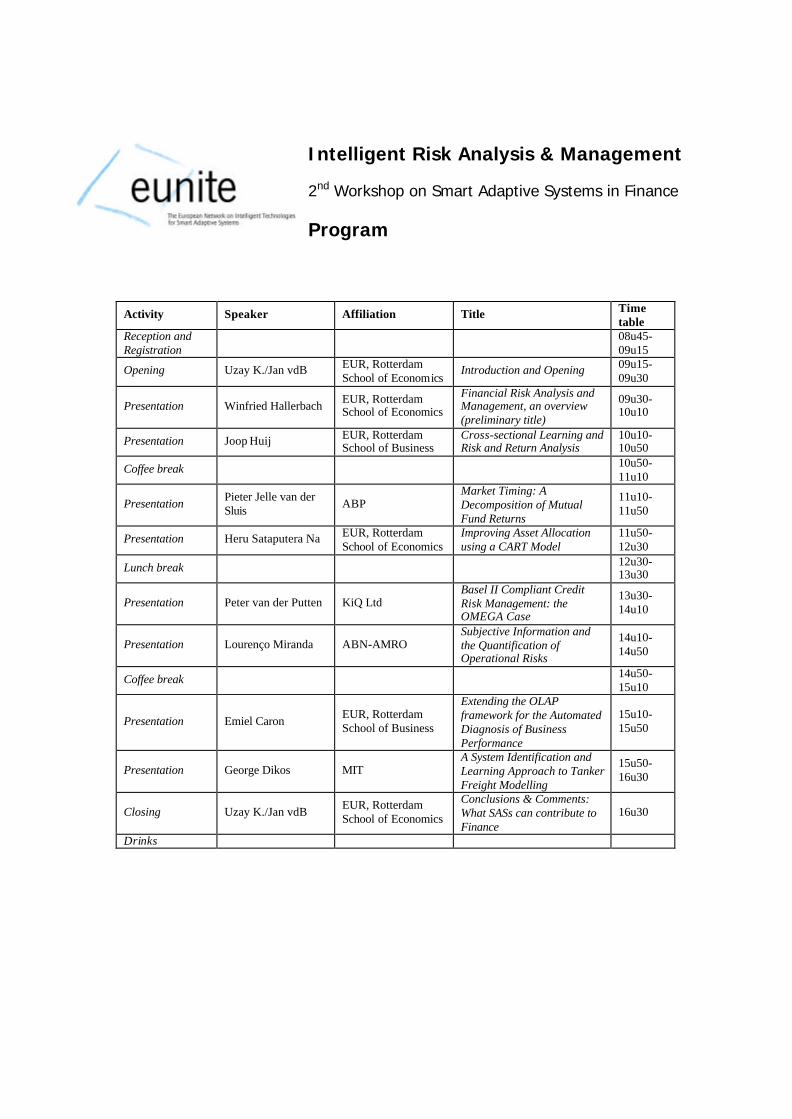
Intelligent Risk Analysis & Management 2nd Workshop on Smart Adaptive Systems in Finance Program

Activity Speaker Affiliation Title Time table

Reception and Registration

08u45- 09u15

Opening Uzay K./Jan vdB EUR, Rotterdam School of Economics

Introduction and Opening 09u15-09u30

Presentation Winfried Hallerbach EUR, Rotterdam School of Economics

Financial Risk Analysis and Management, an overview (preliminary title)

09u30- 10u10

Presentation Joop Huij EUR, Rotterdam School of Business

Cross-sectional Learning and Risk and Return Analysis

10u10-10u50

Coffee break 10u50-11u10

Presentation Pieter Jelle van der Sluis ABP

Market Timing: A Decomposition of Mutual Fund Returns

11u10-11u50

Presentation Heru Sataputera Na EUR, Rotterdam School of Economics

Improving Asset Allocation using a CART Model

11u50-12u30

Lunch break 12u30- 13u30

Presentation Peter van der Putten KiQ Ltd Basel II Compliant Credit Risk Management: the OMEGA Case

13u30- 14u10

Presentation Lourenço Miranda ABN-AMRO Subjective Information and the Quantification of Operational Risks

14u10- 14u50

Coffee break 14u50- 15u10

Presentation Emiel Caron EUR, Rotterdam School of Business

Extending the OLAP framework for the Automated Diagnosis of Business Performance

15u10- 15u50

Presentation George Dikos MIT A System Identification and Learning Approach to Tanker Freight Modelling

15u50- 16u30

Closing Uzay K./Jan vdB EUR, Rotterdam School of Economics

Conclusions & Comments: What SASs can contribute to Finance

16u30

Drinks

Intelligent Risk Analysis & Management 2nd Workshop on Smart Adaptive Systems in Finance Call for papers

Why, Where, and When?

Why: Because of the enormous expansion and increasing complexity of capital markets, the growing number of financial incidents, and the new demands upon the capital regulation of banks (Basel II) Risk Analysis &Management (RA&M) have drawn a lot of renewed attention. There is a high need for transparent, human-understandable models related to the analysis and reliable assessment of all kinds of risk exposures. Ideally these models are also adaptive in the sense that they can be used under changing market conditions and under different financial market circumstances. Smart Adaptive Systems (SASs), which are developed using techniques from the area of 'Computational Intelligence' including (Probabilistic) Fuzzy systems, Neural Networks, Genetic Algorithms, Decision Trees and others, have the potential to offer such better solutions.

Where: Faculty Club, Erasmus University Rotterdam, Burg. Oudlaan 50, Rotterdam, The Netherlands. When: Wednesday, May 19, 2004 (the day before Ascension Day)

Purpose Understanding in which ways smart adaptive systems can contribute to the improvement of existing RA&M practices is considered of key importance and, therefore, the dissemination of knowledge and experience about the smart adaptive systems within this rapidly developing field. The workshop will provide a platform for the academics and professionals in the RA&M sector to exchange ideas, opinions and experience about the opportunities for computational techniques like data mining, neural networks, decision trees, (statistical) fuzzy modeling, evolutionary computation, and combinations of these. The domain focus of the workshop is on the three main types of financial risk namely market risk, credit risk and operational risk. Examples of the state of the art in this field will be shown including recent academic developments and successful applications. To evaluate the (possible) contributions of SASs to the improvement of RA&M, a special session will be organized where the advantages and limitations of the use of intelligent techniques for developing SASs compared to the use of the more traditional, statistics-based approaches will be discussed.

For Who? The workshop targets professionals (both practitioners and researchers) from the financial sector, especially the banking sector and investment groups as well as scientists from departments of finance at universities with research activities in the field of RA&M.

Call for Extended Abstracts The topics to be covered include all kinds of RA&M applications in the area of market risk, credit risk and operational risk. An essential prerequisite is that at least one Computational Intelligence technique should have been employed. Submit your extended abstract (approximately 2 pages) of your contribution by email: [email protected] before April 30, 2004. Submissions should be in .pdf, .ps or .doc format. Notification of acceptance will be sent via email by May 7, 2004. Extended abstracts and presentations will be published in the Proceedings of the 2nd Workshop on Smart Adaptive Systems in Finance.

Organisation and Program Committee dr.ir. Jan van den Berg ([email protected]) and dr.ir. Uzay Kaymak ([email protected]) Dept. of Computer Science, Intelligent Systems in Business Economics, Rotterdam School of Economics, Erasmus University Rotterdam, The Netherlands More information can (soon) be found at our website: http://www.few.eur.nl/few/research/eurfew21/ibe/seminar/

Sponsors This workshop is sponsored by the European Network of Excellence EUNITE, and is supported by the Working Group ‘Information Systems & Economics’ of the Dutch Research School SIKS.

http://www.facultyclub.nl/

http://web.eur.nl/english/

mailto:[email protected]



http://www.few.eur.nl/few/research/eurfew21/ibe/index.htm

http://www.few.eur.nl/few/english/

http://www.few.eur.nl/few/research/eurfew21/ibe/seminar/

http://www.eunite.org/eunite/index.htm

http://www.siks.nl/

Page 1

Project funded by the Future and Emerging Technologies arm of the IST ProgrammeFET K.A. line-8.1.2 Networks of excellence and working groups


the European Network of Excellence on Intelligent Technologies for

Smart Adaptive Systems





IntroductionOn 1 January 2001, EUNITE - the European Network ofExcellence on Intelligent Technologies for Smart AdaptiveSystems - has started.

It is funded by the Future and Emerging Technologies arm of the IST Programme FET K.A. line-8.1.2 Networks of excellence and working groups

On 1 January 2001, EUNITE - the European Network ofExcellence on Intelligent Technologies for Smart AdaptiveSystems - has started.


Page 2



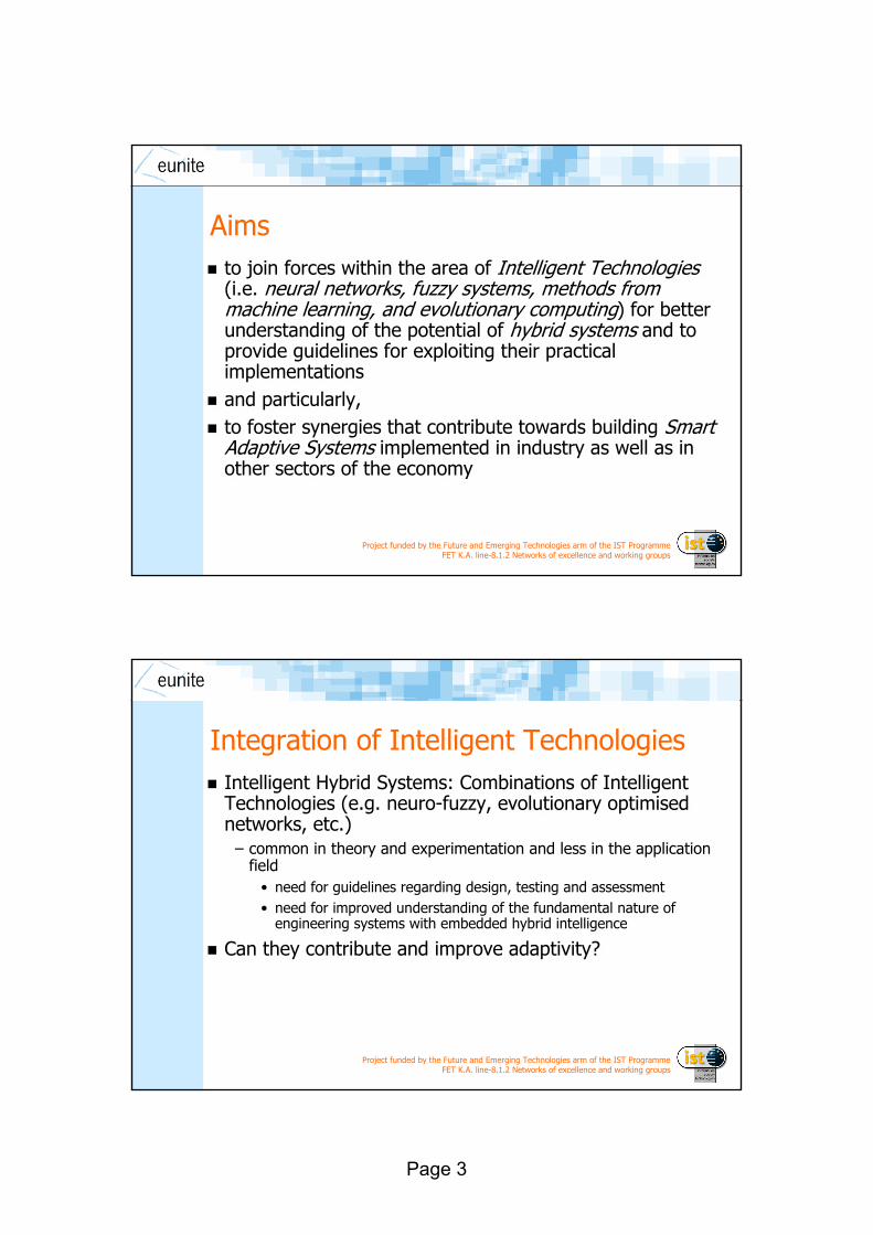
Aimsto join forces within the area of Intelligent Technologies(i.e. neural networks, fuzzy systems, methods from machine learning, and evolutionary computing) for better understanding of the potential of hybrid systems and to provide guidelines for exploiting their practical implementationsand particularly,to foster synergies that contribute towards building SmartAdaptive Systems implemented in industry as well as in other sectors of the economy.

to join forces within the area of Intelligent Technologies(i.e. neural networks, fuzzy systems, methods from machine learning, and evolutionary computing) for better understanding of the potential of hybrid systems and to provide guidelines for exploiting their practical implementationsand particularly,to foster synergies that contribute towards building SmartAdaptive Systems implemented in industry as well as in other sectors of the economy.



Integration of Intelligent TechnologiesIntelligent Hybrid Systems: Combinations of Intelligent Technologies (e.g. neuro-fuzzy, evolutionary optimised networks, etc.)

– common in theory and experimentation and less in the applicationfield

• need for guidelines regarding design, testing and assessment • need for improved understanding of the fundamental nature of

engineering systems with embedded hybrid intelligence.

Can they contribute and improve adaptivity?

Intelligent Hybrid Systems: Combinations of Intelligent Technologies (e.g. neuro-fuzzy, evolutionary optimised networks, etc.)



engineering systems with embedded hybrid intelligence.


Page 3



Smart Adaptive SystemsAdaptivity:

A system is adaptive if it can adequately perform even in non-stationary environments, where significant smooth changes of themain data characteristics can be manifested.

Examples:monitoring systems in the presence of tool wearmedical diagnostic systems in the presence of a changing populationforecasting of dynamically changing time series

Adaptivity is also a request in the sense of portability and reusability as minimises the effort for re-development..

Example:monitoring or diagnostic systems that should run on different machines which are of similar type but each have their individual characteristics.

Adaptivity:A system is adaptive if it can adequately perform even in non-stationary environments, where significant smooth changes of themain data characteristics can be manifested.

Examples:monitoring systems in the presence of tool wearmedical diagnostic systems in the presence of a changing populationforecasting of dynamically changing time series

Adaptivity is also a request in the sense of portability and reusability as minimises the effort for re-development..

Example:monitoring or diagnostic systems that should run on different machines which are of similar type but each have their individual characteristics.



Activities• Roadmap • Organise Conferences-Symposia-Workshops• Disseminate Feasibility and Joint case studies on

hybrid and Smart Adaptive Systems• Provide best practice guidelines - best Methodology• Learning Center• Patent support - IPR service• Benchmarking-Competitions • Scientific e-archives, e-Dictionary • Newsletter• WWW site

• Roadmap • Organise Conferences-Symposia-Workshops• Disseminate Feasibility and Joint case studies on

hybrid and Smart Adaptive Systems• Provide best practice guidelines - best Methodology• Learning Center• Patent support - IPR service• Benchmarking-Competitions • Scientific e-archives, e-Dictionary • Newsletter• WWW site

Page 4



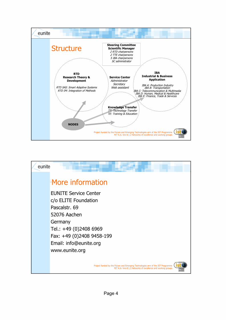
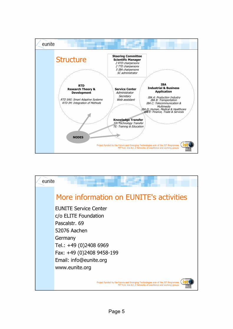
Steering CommitteeScientific Manager

2 RTD chairpersons2 TTE chairpersons5 IBA chairpersonsSC administrator

IBAIndustrial & Business

Application

IBA A: Production IndustryIBA B: Transportation

IBA C: Telecommunication & MultimediaIBA D: Human, Medical & Healthcare

IBA E: Finance, Trade & Services

Service CenterAdministrator

SecretaryWeb assistant

NODES

RTDResearch Theory &

Development

RTD SAS: Smart Adaptive SystemsRTD IM: Integration of Methods

Knowledge Transfer TT: Technology TransferTE: Training & Education

Structure



More informationEUNITE Service Centerc/o ELITE FoundationPascalstr. 6952076 AachenGermanyTel.: +49 (0)2408 6969Fax: +49 (0)2408 9458-199Email: [email protected]

EUNITE Service Centerc/o ELITE FoundationPascalstr. 6952076 AachenGermanyTel.: +49 (0)2408 6969Fax: +49 (0)2408 9458-199Email: [email protected]

ABSTRACTS OF CONTRIBUTIONS

Financial Risk Analysis & Management: An Overview The globalization of business paired with rapid technological changes and increased volatility in the financial markets has changed the risk profiles of many companies dramatically. Firms have responded by embracing the concept of financial risk management. Mitigating or neutralizing excess risk exposures through hedging is widespread corporate practice nowadays. As a preamble to the various presentations today, we provide a concise overview of the various stages of the enterprise-wide risk management process, viz. risk analysis, policy formulation, implementation, and performance evaluation. We devote special attention to model risk, cognitive biases in decision making under uncertainty, and the link between the decision context and performance evaluation. ------------------------------------------------------------------------------------ Dr. Winfried G. Hallerbach Home: Hoflaan 93, NL-3062 JD Rotterdam, The Netherlands phone: +31 (10) 411-0899 Work: Dept of Finance, Erasmus University Rotterdam POB 1738, NL-3000 DR Rotterdam, The Netherlands phone: +31 (10) 408-1290 fax: +31 (10) 408-9165 e-mail: [email protected] http://www.few.eur.nl/few/people/hallerbach http://www.finance-on-eur.nl

Cross-Sectional Learning and Risk and ReturnAnalysis

Joop Huij∗

May 6, 2004

Traditional estimates of risk and return measures are hampered by potentially

high levels of inaccuracy, particulary when only short horizons of monthly returns

are used. With only a small number of observations available, it is notoriously

difficult to separate skill from random luck. For example, investment funds that

are less well-diversified and have higher levels of non-systematic risk experience a

larger probability to end up with an extreme ranking because managers of these

funds typically place larger bets, i.e. run higher risks. Consequently, top and

bottom deciles in performance rankings will to a large extent be attributable to

random luck rather than managerial skill, and are therefore not very useful for

analyzing market efficiency, or fund picking purposes.

In this study, we evaluate several smart systems that not only base estimates

of risk and return measures on available returns histories, but also incorporate

economic knowledge. For example, studies by among Elton et al. (1993) and

Carhart (1997) indicate that funds with higher fees typically underperform those

with lower fees. By means of a Bayesian framework, one could exploit prior infor-

mation related to expenses of funds, and investors’ beliefs about managerial skills

(see Baks et al. (2001), Pastor and Stambaugh (2002a,b)). In this framework,

raw performance estimates are shrunk towards the funds’ expenses conditional on

how strongly one beliefs in managerial skill. Another example are adjusted beta

estimates that are provided by commercial information services like Bloomberg.

Hereby, one exploits the knowledge that (by construction) the expected average

∗Dept. of Financial Management, Erasmus University Rotterdam, The Netherlands,[email protected].

value of betas of a cross-section of stocks is equal to one. Raw beta estimates are

then adjusted in the sense that they are shrunk towards this value of one. More

generally, the use of Bayesian shrinkage techniques can be motivated purely on

the basis of statistical arguments: When a cross-section of risk and return esti-

mates is considered, extreme values are more than average subject to positive and

negative estimation errors, respectively, and shrinking them towards an expected

value may result in more accurate inferences.

The setup of the study is as follows: First, we formulate the most general

form of the Bayesian system, and provide several applications of this framework,

e.g. CAPM, and Fama-French model (Fama and French, 1992, 1993). We then

review current literature on additional information that is incorporated in the

estimation procedure, and discuss the relative strengths and weaknesses of these

implementations. Furthermore, we extend our model so that prior beliefs become

adaptive in the sense that they can shift over time, and adjust to market dynam-

ics and structural shifts. Second, we consider a range of alternative approaches

to estimate our model (hyper)parameters, including maximum likelihood, (iter-

ative) empirical Bayes, expectation maximization, and Gibbs sampling. Third,

we evaluate accuracy and ranking ability of traditional and Bayesian estimators

under controlled circumstances, by means of a Monte Carlo simulation. Our re-

sults demonstrate that the gains in accuracy and ranking abilities are substantial

and robust over different model specifications and measurement horizons. For ex-

ample, Bayesian alphas appear to be about 50 percent more accurate in term of

root mean squared error when evaluating a 12-month time period. Also, rankings

based on these estimates are significantly better; not only in statistical terms such

as correlation with true rankings, but also from an economic perspective in the

sense that the funds that are rated as top-performers have substantially higher

true alphas and Sharpe ratios. Finally, we apply Bayesian alphas to investigate

short-run predictability in fund returns for a large sample of US equity funds.

References

K. Baks, A. Metrick, and J. Wachter. Should investors avoid all actively managed

mutual funds? a study in bayesian performance evaluation. The Journal of

2

Finance, 56:45–85, 2001.

M. Carhart. On persistence in mutual fund performance. The Journal of Finance,

52:57–82, 1997.

E. J. Elton, M. J. Gruber, S. Das, and M. Illavka. Efficiency with costly infor-

mation: A reinterpretation of evidence from managed portfolios. The Review

of Financial Studies, 6:1–22, 1993.

E. F. Fama and K. R. French. The cross-section of expected stock returns. The

Journal of Finance, 47:427–465, 1992.

E. F. Fama and K. R. French. Common risk factors in the returns on stocks and

bonds. Journal of Financial Economics, 33:3–56, 1993.

L. Pastor and R. Stambaugh. Mutual fund performance and seemingly unrelated

assets. Journal of Financial Economics, 63:315–349, 2002a.

L. Pastor and R. F. Stambaugh. Investing in equity mutual funds. Journal of

Financial Economics, 63:351–380, 2002b.

3


Chi Lok Cheung, Heru Sataputera Na, Jan van den Berg

Erasmus University Rotterdam

Department of Computer Science Room H9-19, P.O. Box 1738

3000DR Rotterdam, The Netherlands Email: [email protected], [email protected],

[email protected]

Abstract

Based on a case offered by ROBECO, we compare three strategies for improving the performance of a Fund Manager who tries to gain a better return on investments by temporarily deviating from the standard investment strategy given by a client. The analysis is based on the construction of a decision tree (CART). The main goals of this work can be formulated as follows:

• To get insight in the importance of the relevant ' indicator variables', • To improve performance by intelligently adapting the investment strategy.

Elaboration: The return as obtained by applying the client’s investment strategy is termed the standard return. The standard strategy for this case concerns a strategy with 50% investment in equities and 50% investments in fixed income. The fund manager is allowed to deviate temporarily from the standard strategy provided that – on average – the investments are still about 50% in equities and 50% in fixed income. To simplify matters, the deviating strategies used here are either 100% investment in equities and 100% investment in fixed income. In this way, the problem becomes to find out under which circumstances (input conditions) what type of strategy should be chosen, i.e., investments in either 100% equities (strategy 1), 50% equities and 50% fixed income (strategy 2), or 100% fixed income (strategy 3). The available data set concerns a set of indicator variables which are assumed to be related to the next month return rates of investments in equities and in fixed income. All together, 279 month’ records are available. Let the excess return ER(m) in month m be defined as

),()()( mRmRmER FIEQ −= (1)

where )(mREQ is the return from investments in equities and )(mRFI represents the return from investments in fixed income (in month m). The historical Excess Returns ER(m) can be calculated from the given data set and are shown in the next figure:

-25.000%

-20.000%

-15.000%

-10.000%

-5.000%

0.000%

5.000%

10.000%

15.000%

1 18 35 52 69 86 103

120

137

154

171

188

205

222

239

256

273

Series1

In case ER(m+1) (excess return in the next month) is expected to be positive, it is reasonable to apply strategy 1, in case ER(m+1) ≈ 0, strategy 2 is most appropriate, and if ER(m+1) is negative, strategy 3 is best. To implement this idea, we have introduced a threshold range α (0 ≤ α ≤. 1) that determines two cut-off points of excess returns. The corresponding investment decision rule can be summarized as follows: If Expected ER(m+1) > (1+α)/2 Then 'Select Strategy 1', If Expected ER(m+1) < (1-α)/2 Then 'Select Strategy 3', Else 'Select Strategy 2'. E.g., if α = 0.2, the corresponding cut-off points are 0.4 and 0.6. Consequently, if the expected ER() belongs to the 40% lowest excess returns observed, strategy 3 is chosen, if it belongs to the 40% highest excess returns, strategy 1 is chosen, otherwise strategy 2 is chosen. It should be clear that the selection of the strategy to be applied (in the next month) depends on α. One of the main goals of our research efforts has been to find the optimal value of α. The optimal decision strategy has been induced from the data by trying various α-values where the CART algorithm [1] has been used in order to (a) first learn and to (b) second predict (classify) the right strategy. During the presentation, the details of the approach will be shown. In practice, changing strategy involves transaction costs that should be taken into account. These transaction actions are indeed taken into account when we calculated the performance of each system developed. In addition, 10-fold cross validation has been applied in order to investigate the stability of our approach. Results: We will conclude the presentation by showing the precise results. Among other things, we found that a threshold value of about α = 0.32 yields the expected best investment decisions. We will also show the corresponding decision trees. In the near future, all results will be discussed with the domain experts. References:

[1] Breiman, et al. (1993). Classification and Regression Trees, Chapman and Hall, Boca

Raton.

[2] Help files van Statistics Toolbox, Matlab

[3] Mitchell, T. M. (1997). Machine Learning, McGraw–Hill International Editions,

Computer Science Series, p. 63

[4] Quinlan, J. R. (1986). Induction of Decision Trees. Machine Learning, 1(1), p. 81-

106

[5] Quinlan, J. R. (1993). C4.5: Programs for Machine Learning. San Matteo, CA:

Morgan Kaufmann.

Basel II Compliant Credit Risk Management: the OMEGA Case

Peter van der Putten KiQ Ltd

& LIACS, Leiden University

Arnold Koudijs KiQ Ltd

De Lairessestraat 150 1075 HL Amsterdam,

The Netherlands {peter.van.der.putten,

arnold.koudijs, rob.walker} @ kiq.com

Rob Walker KiQ Ltd

ABSTRACT In this paper we highlight some high level requirements for adaptive modelling in a BASEL II credit risk context and highlight the OMEGA approach as a case example for BASEL II compliant risk management. We conclude with a vision on the future of adaptive ratings, models and enterprises.

Keywords Rating models, credit risk, Basel II, computational intelligence, adaptive systems

1. Introduction The new BASEL Accord (BASEL II) aims to make regulatory capital requirements more sensitive to risk to improve the overall stability of the financial market. BASEL II covers credit, market and operational risk. For calculating and managing credit risk, banks can follow the so-called Internal Ratings-Based approach (IRB), which allows calculation of risk ratings based on models developed by the bank on its own data [1].

Of course, the procedures for developing, deploying and monitoring these models must meet certain requirements, some of which are specified explicitly by BASEL II and some of which are implied by it. In section 2 we will highlight a selection of these requirements. Next, the OMEGA Active Decision Management Suite will be discussed as a case example of a state of the art solution for implementing a managed BASEL II credit risk management process (section 3). In addition we identify some opportunities that are related to BASEL II, beyond mere compliancy (section 4). Finally we specifically address some of the no-go areas and opportunities for adaptive control (section 5).

2. IRB Requirements The Internal Ratings-Based (IRB) approach depends on so-called risk components to calculate the expected loss for each exposure, which in turn sum up to the total credit risk. Basel II dictates that the capital requirements are not only based on the expected losses but also on the sophistication of the methods used to estimate these losses. The more advanced the methods used, the better a bank can do in reducing the minimum capital requirements. Expected loss is defined as

EL= PD x LGD x EAD x M (1)

with PD the probability of default, LGD the loss given default, EAD the exposure at default and M the maturity of the exposure. Typically, under the so-called IRB Foundation approach, banks provide their own estimates of PD and use supervisory estimates for other risk components – in the Advanced IRB approach all components are estimated by the bank itself.

Basel compliant ratings must be calculated on the basis of at least two years of data, so the availability of historic data over that period is a must have. The data must be analyzed to calculate ratings that properly reflect the risk in a portfolio. Historically, classical statistical methods like regression are used for estimating risk components. However, the BASEL II standard does not require a specific modeling algorithm to be used, but these must meet a number of criteria. Merely being predictive is not good enough. The models must be proven to be stable under varying economic conditions and over various points in time. A priori risk assessment knowledge that may improve the bottom-up risk models must be incorporated where possible.

3. The OMEGA Approach Originally, the focus of OMEGA was purely on predictive model development for credit risk management using genetic algorithms [5]. Then OMEGA developed into a full decision management suite for optimising the entire customer relationship, including risk. OMEGA provides managed process support for the steps after a model has been developed: linking models with business rules into a decision logic, batch and real-time decision logic deployment and monitoring [2,3,4].

3.1 Model Development Process BASEL II requires that best practices for developing rating models are followed, to minimize the scope for errors and ensure consistent quality. In our opinion, the best way to ensure this is to hardcode this process in the model development tool and to provide automated support where possible, without sacrificing user control. This should not be limited to the core model algorithms, but also include project definition, data preparation and model evaluation. Because of this model factory approach, model accuracy, - robustness and process compliancy are optimized and a full audit trail to the development process can be provided. Projects can also be saved to best practice templates. As core modelling algorithms, logistic regression, additive scorecards, decision trees and genetic algorithms are available, to cover the whole spectrum between simple, understandable models and more powerful, complex models.

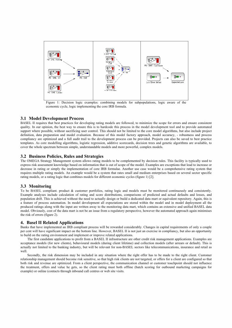
3.2 Business Policies, Rules and Strategies The OMEGA Strategy Management system allows rating models to be complemented by decision rules. This facility is typically used to express risk assessment knowledge based on information that is out of scope of the model. Examples are exceptions that lead to increase or decrease in rating or simply the implementation of core IRB formulae. Another use case would be a comprehensive rating system that requires multiple rating models. An example would be a system that rates small and medium enterprises based on several sector specific rating models, or a rating logic that combines models for different economic cycles (figure 1) [2].

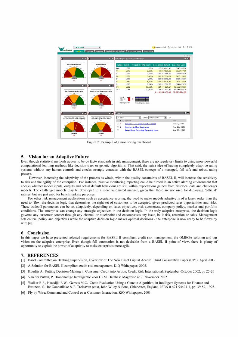
3.3 Monitoring To be BASEL compliant. product & customer portfolios, rating logic and models must be monitored continuously and consistently. Example analyses include calculation of rating and score distributions, comparisons of predicted and actual defaults and losses, and population drift. This is achieved without the need to actually design or build a dedicated data mart or equivalent repository. Again, this is a feature of process automation. In model development all expectations are stored within the model and in model deployment all the produced ratings along with the input are written away to the monitoring data mart, which contains an extensive and unified BASEL data model. Obviously, cost of the data mart is not be an issue from a regulatory perspective, however the automated approach again minimises the risk of errors (figure 2).

4. Basel II Related Applications Banks that have implemented an IRB compliant process will be rewarded considerably. Changes in capital requirements of only a couple per cent will have significant impact on the bottom line. However, BASEL II is not just an exercise in compliancy, but also an opportunity to build on the rating environment and implement or improve related applications.

The first candidate applications to profit from a BASEL II infrastructure are other credit risk management applications. Examples are acceptance models (for new clients), behavioural models (during client lifetime) and collection models (after arrears or default). This is actually not limited to the banking industry, but will be relevant for non-BASEL sectors like telecommunications, insurance and retail as well.

Secondly, the risk dimension may be included in any situation where the right offer has to be made to the right client. Customer relationship management should become risk sensitive, so that high risk clients are not targeted, or offers for a client are configured so that both risk and revenue are optimized. From a client perspective, the communication channel or customer touchpoint should not influence the treatment, offers and value he gets, so the client rating must both offline (batch scoring for outbound marketing campaigns for example) or online (contacts through inbound call centres or web site visits.

Figure 1: Decision logic examples: combining models for subpopulations, logic aware of the economic cycle, logic implementing the core IRB formula.

5. Vision for an Adaptive Future Even though statistical methods appear to be de facto standards in risk management, there are no regulatory limits to using more powerful computational learning methods like decision trees or genetic algorithms. That said, the naive idea of having completely adaptive rating systems without any human controls and checks strongly contrasts with the BASEL concept of a managed, fail safe and robust rating process.

However, increasing the adaptivity of the process as whole, within the quality constraints of BASEL II, will increase the sensitivity to risk and the agility of the enterprise. For instance, passive monitoring reporting could be turned in an active alerting environment that checks whether model inputs, outputs and actual default behaviour are still within expectations gained from historical data and challenger models. The challenger models may be developed in a more automated manner, given that these are not used for deploying ‘official’ ratings, but are just used for benchmarking purposes.

For other risk management applications such as acceptance scoring, the need to make models adaptive is of a lesser order than the need to ‘flex’ the decision logic that determines the right set of customers to be accepted, given predicted sales opportunities and risks. These tradeoff parameters can be set adaptively, depending on sales objectives, risk averseness, company policy, market and portfolio conditions. The enterprise can change any strategic objectives in the decision logic. In the truly adaptive enterprise, the decision logic governs any customer contact through any channel or touchpoint and encompasses any issue, be it risk, retention or sales. Management sets course, policy and objectives while the adaptive decision logic makes optimal decisions - the enterprise is now ready to be flown by wire [6].

6. Conclusion In this paper we have presented selected requirements for BASEL II compliant credit risk management, the OMEGA solution and our vision on the adaptive enterprise. Even though full automation is not desirable from a BASEL II point of view, there is plenty of opportunity to exploit the power of adaptivity to make enterprises more agile.

7. REFERENCES [1] Basel Committee on Banking Supervision, Overview of The New Basel Capital Accord. Third Consultative Paper (CP3), April 2003 [2] A Solution for BASEL II compliant credit risk management. KiQ Whitepaper, 2003. [3] Koudijs A., Putting Decision-Making in Consumer Credit into Action, Credit Risk International, September-October 2002, pp 25-26 [4] Van der Putten, P. Broodnodige Intelligentie voor CRM. Database Magazine nr 7, November 2002. [5] Walker R.F., Haasdijk E.W., Gerrets M.C. Credit Evaluation Using a Genetic Algorithm, in Intelligent Systems for Finance and

Business, S. In: Goonatilake & P. Treleaven (eds), John Wiley & Sons, Chichester, England, ISBN 0-471-94404-1, pp. 39-59, 1995. [6] Fly by Wire: Command and Control over Customer Interaction. KiQ Whitepaper, 2001.

Figure 2: Example of a monitoring dashboard

A System Identification and LearningApproach to Tanker Freight Modelling

George Dikos ∗

Massachusetts Institute of Technology

May 2, 2004

∗[email protected]

1

AbstractIn this paper we use a System Identification approach for the specification

and estimation of the evolution of freight rates for tanker carriers. Wederive the parametric form of the modules of the system from first

principles and employ Economic Theory, in order to reduce thedimensionality of the problem and allow for the control of different policies

on heterogenous agents. We aggregate actions by individual agents andform the structural equations that determine the modules of the system.

By combining statistical analysis and economic insight, we achieveidentification of the system and fully track the directional changes in freight

rates. We then proceed with performance evaluation and conclude withdiscussing dynamic learning, as well as a hybrid model that maximizes the

performance of the system, both within and out-of-sample. Finally, weaddress issues of consistency and stability of the system in a framework,

where data arrive dynamically.

1 Introduction

Two are the main objectives of this paper: We develop a structural modelfor time charter rates in the oil tanker industry, using system modellingtechniques. While pursuing this task we demonstrate how system dynamicsand system identification techniques can effectively model complex systems,where agents undertake economic actions and challenge the widespread per-ception that namely, structural models consistently under-perform statisticalmodels.

Since the seminal work of Lucas and Prescott [?] the General Equilibriumapproach has been the predominant structural model for the interaction ofeconomic agents under perfect competition. Due to the strict requirementson the rationality of agents and their ability to commit themselves to fullyrational decisions, the General Equilibrium approach has severe implicationson price dynamics, especially when we try to compute the equilibrium incomplex markets, such as the oil tanker industry. Besides the inability ofmost structural models to over-perform statistical models, economists havebeen particularly cautious with models that do no take into account the abil-ity of agents to “learn” and adapt their optimal policies dynamically. Afterwhat is formally known as Lucas’ critique [?], recursive methods have beenthe standard structural modelling technique. Besides our ultimate goal of de-

2

signing a system that will adequately explain the evolution of tanker freightrates, we go one step further and provide the necessary theoretical reasoningthat will hopefully make the case for employing system dynamics and systemidentification and estimation techniques in the process of modelling complexenvironments with interacting agents.

Before proceeding with implementing our tasks let us re-address the theo-retical issues of system modelling and their empirical relevance in the specificmarket for time charter freight rates. As we discussed earlier, there have beentwo main shortcomings that have not allowed System Identification to be-come the main device towards the modelling of complex economic systemsof interacting agents, despite the natural tendency of economic systems todeviate around a trend: On the one hand the system identification and mod-elling approach suffers inherently from Lucas’ critique [?]. Using the system,in order to account for the effect of different policies, does not take intoconsideration the adverse effects of these policies on the optimal responsesof agents and on the specific modules of the system. Furthermore, most ofthe modules employed are not derived on “first principles”, which does notallow policy makers to control for external events and furthermore does notincorporate the dynamic nature of economic systems. More specifically, themodules of the system are usually derived ad hoc and do not take into ac-count the ability of agents to learn and converge to optimal policies, underthe absence of arbitrage opportunities.

Furthermore, from an empirical point of view the models derived on theprinciples of structural systems have not been able to outperform the sta-tistical models employed in financial applications, such as the GeneralizedAuto Regressive Conditional Heteroscedastic family of models [?]. Due tothe dynamic response of agents to shifts in policy and external shocks, eco-nomic systems are time varying, which implies that even the dimension ofthe system changes over time. Non-parametric solutions may lead to a se-vere over-parametrization of the system and in some sense, if we attempt tofully identify the system non-parametrically, there is no need for economic orscientific intuition. In this paper we demonstrate that despite the fact thatany attempt to model economic systems without theory and first principlesin the background, leads to overparametrization, system theory coupled witheconomics may provide a useful alternative towards the understanding andmodelling of complex economic systems.

The paper is organized as following: We start discussing how EconomicTheory may provide helpful intuition into the case of economic systems with

3

interacting agents, whilst providing the necessary framework for a consis-tent mathematical formulation of the modules of the system, with respectto the equilibrium laws of the neoclassical economic theory. On the agentmicro-level, economics coupled with assumptions of exogeneity allow us toavoid the shortcomings of Lucas’ critique [?] and significantly reduce thedimensionality of the problem. We then proceed and re-address themathematical formulation of the System Identification problem and expandon the interrelated issues of consistency and stability. Finally, we discuss ourempirical results, regarding the modelling of time charter freight rates in thetanker industry and develop an empirical case that clearly outperforms theexisting statistical models. We conclude discussing Hybrid Models that in-tegrate both trends in modelling economic systems. Before proceeding withthese tasks we briefly introduce the tanker market industry and discuss themain characteristics of this market, such as the adverse driving forces andfeedback effects.

4

References

[1] Coyle, R. G. (1978). “A System Dynamics Case Study”. Journal of Op-erational Research 2, 2, pp. 86-96.

[2] Dikos, G. (2004). “Decisionmetrics: Dynamic Structural Estimation ofShipping Investment Decisions”. Unpublished PhD Thesis, Departmentof Ocean Engineering, Massachusetts Institute of Technology.

[3] Dixit A. and R. Pindyck (1994). “Investment under Uncertainty”.Princeton University Press.

[4] Grammenos, C. (2002).

[5] Khaled, A., AbbasMichael G. and H. Bell (1994). “System Dynamics Ap-plicability to Transportation Modelling”. Transportation Research PartA: Policy and Practice 28, 5, pp. 373-390.

[6] Sharp, J. and D.H.R. Price (1984). “System Dynamics and OperationalResearch: An Appraisal”. European Journal of Operational Research 16,pp. 1-12.

5

Extending the OLAP framework for the automated diagnosis of business performance

Emiel Caron1 (presenter), Hennie Daniels 1,2

1Erasmus University Rotterdam, ERIM Institute of Advanced Management Studies, PO Box 90153, 3000 DR Rotterdam, The Netherlands, phone +31 010 4082574, e-mail: [email protected]; 2Tilburg University, CentER for Economic Research, Tilburg, The Netherlands

Short abstractThe purpose of OLAP (On-Line Analytical Processing) systems is to provide a framework for the (risk) analysis of multidimensional data. Many tasks related to analysing multidimen-sional data and making business decisions are still carried out manually by analysts (e.g. financial analysts, accountants, or business managers). An important and common task in multidimensional analysis is business diagnosis. Diagnosis is defined as finding the “best” explanation of observed symptoms. Today’s OLAP systems offer little support for automated diagnosis of business performance. This functionality can be provided by extending the conventional OLAP system with an explanation formalism, which mimics the work ofbusiness decision makers in diagnostic processes. The central goal of this presentation is the identification of specific knowledge structures and reasoning methods required to construct computerized explanations from multidimensional data and business models. Recently, an explanation formalism was developed that generates explanations on the basis of simple business models. This explanation formalism serves as a starting point for more complex automated diagnosis in the OLAP framework. We propose an algorithm that generatesexplanations for symptoms in multidimensional business data. The algorithm was tested on a fictitious case study involving the comparison of financial results of a firm’s business units.

OLAP introductionDatabases systems are the core component of OLTP (On-Line Transaction Processing)systems, which support operational business processes. In general, OLTP systems are poorly suited for decision support. Efforts to extract analytical information from OLTP databases result in complex queries, multiple joins, and large computation times. To support business decision-making OLAP is a powerful and adaptive technology. OLAP is defined as “acategory of software technology that enables analysts, managers and executives to gaininsight into data through fast, consistent, interactive access to a wide variety of possible views of information that has been transformed from raw data to reflect the real dimensionality of the enterprise as understood by the user” [3].

The core component of an OLAP system (or data cube) is the data warehouse, which is decision-support database that is periodically updated by extracting, transforming, and loading data from several OLTP databases. An OLAP system organizes data using the dimensional modelling approach, which classifies data into measures and dimensions.Measures or facts (e.g. sales figures, or costs) are the basic units of interest fo r analysis. Measures represent countable or summable information concerning a business process.Dimensions are the different perspectives for viewing measures. Dimensions are (can be) organised as dimension hierarchies, which offers the possibility to view measures at different dimension levels (e.g. month quarter year≺ ≺ ). The hierarchies in a dimension specify the aggregation levels.

General model for automated diagnosis of business performanceThe formalisation of diagnostic problem-solving is a sub-area of Operations Research (OR) and Artificial Intelligence (AI). In [2] diagnosis is defined as finding the best explanation of

observed abnormal behaviour of a system under study. In this paper we take a model basedrather, as opposed to heuristic classification, approach to knowledge representation. Inaddition we take a causal view of explanation that is able to deal with quantitative phenomena that pervade the domain of business, finance, accounting, and logistics.

According to a causal model of explanation, phenomena (events) are explained by giving their causes. In this research paper the exposition on diagnostic reasoning and causal explanation is largely based on Feelders and Daniels’ notion of explanations [1, 2], which is again based on Humpreys’ notion of aleatory explanations. Causal influences can appear in two forms: contributing and counteracting. Therefore, Humphreys proposes the following canonical form for causal explanations:

Event E occurred because of C+ , despite C− ,

where E is the event to be explained, C+ is non-empty set of contributing causes, and C− a (possibly empty) set of counteracting causes. The explanation itself consists of the causes to which C+ jointly refers. C− is not part of the explanation of E, but gives a clearer notion of how the members of C+ actually brought about E . The event E can be specified as a variable y changing value from time t to t´.

The explanandum introduced by Feelders and Daniels is a three-place relation, ,a F R⟨ ⟩ between an object a (e.g. the ABC-company), a property F (e.g. having a low profit)

and a reference class R (e.g. other companies in the same branch or industry). Here the event E is thus replaced by a more detailed explanandum. The task is not to explain why a has property F, but rather to explain why a has property F when the members of R do not . As we shall see, there are some typical ways to construct reference classes. For the purpose of explanation, the class R can often be reduced to one member r, which is in some sense the average of the class R or the ideal object. The syntax of an explanation reads:

, ,a F r⟨ ⟩ because C+ , despite C− ,

where C+ is a non-empty set of contributing causes, and C− is a (possibly empty) set of counteracting causes.

Two principal knowledge representation structures for diagnosis of business performance are identified:

• Knowledge of general laws expressing relations and variables between events: the businessmodel M. The bus iness model M represents quantitative financial and operating variablesby means of mathematical equations of the form: ( )y f= x where 1( , , )nx x=x … .

• Knowledge of the “normal” behaviour of objects: the norm model (the reference object r).Common “reference objects” for the diagnosis of business performance are, for example,historical norm values, industry averages, or plans and budgets as norm values.

Extending OLAP with explanation capabilities We extend the method of explanation for the purpose of diagnosis of business performancewith explanation capabilities. Or stated differently we adapt the explanation model in such a way that it can deal with multidimensional financial data and can generate explanations for it.In multidimensional data there are two possible explanation directions: namely an explanation direction in the right-hand side of the business model equations (the measures) and anexplanation direction in the right-hand side of the drilldown equations (the dimensions).

To make the connection with the explanation model we have to define the actual object a and the reference object r as multidimensional objects with, for example, a time, location, or product dimension. Therefore, we associate the objects a and the reference objects r of the explanandum with the dimension vector d. In addition, the property F of the explanation model is related to the measure attribute of the multidimensional model. The actual object a(d) in combination with the property F expresses a cell of the data cube that needs to be explained. The property F in combination with the reference model r(d) expresses the cell of reference on the data cube. We are interested in explaining the difference between the actual multidimensional object and a multidimensional reference object. Consequently, we have to explain the following type of events in the data cube:

• a(d) = the actual multidimensional object;• F = a particular measure (variable) deviates from its norm value;• r(d) = the multidimens ional reference object.

We use the idea of progressive deepening in the construction of a maximal explanationalgorithm for multidimensional data. Such an algorithm is needed to create multi- levelexplanations. For diagnostic purposes it is useful to continue an explanation of ( )y q∂ =d

where { }low,highq = , by explaining the qualitative differences between the actual and norm

values of its contributing causes. This process can be continued until a contributing cause is encountered that cannot be explained:

• within the business model, because the business model equations do not contain a relation in which this contributing cause appears on the left-hand side, and

• within the dimensions, because the drilldown equations do not contain a summarization relation in which this contributing cause appears on the left-hand side.

The algorithm was tested on a fictitious case study involving the comparison of financial results of a firm’s business units.

References[1] A.J. Feelders, “Diagnostic reasoning and explanation in financial models of the firm”,

PhD thesis, University of Tilburg, (1993).[2] H.A.M. Daniels, A.J. Feelders, “Theory and methodology: a general model for

automated business diagnosis”, European Journal of Operational Research, 130: 623-637, (2001).

[3] OLAP Council, http://www.olapcounsil.org, (2000).[4] A. Datta, H.Thomas, “The cube data model: a conceptual model and algebra for on-

line analytical processing in data warehouses”, Decision Support Systems, 27 (3): 289-301, (1999).

[5] A. Shoshani, “OLAP and statistical databases: Similarities and differences”, InSixteenth ACM SIGACT SIGMOD SIGART Symp. on Principles of DatabaseSystems, pages 185-196, (1997).

PRESENTATIONS

Page 1



2nd Workshop Smart Adaptive Systems in Finance2nd Workshop Smart Adaptive Systems in Finance

Focus: Intelligent Risk Analysis & Management

19 May 2004

Erasmus University RotterdamThe Netherlands

Supported by

Focus: Intelligent Risk Analysis & Management

19 May 2004

Erasmus University RotterdamThe Netherlands

Supported by



AgendaEUNITESIKSFirst WorkshopProgram of Today

EUNITESIKSFirst WorkshopProgram of Today

Page 2









IntroductionOn 1 January 2001, EUNITE - the European Network of Excellence on Intelligent Technologies for Smart Adaptive Systems - has started.


On 1 January 2001, EUNITE - the European Network of Excellence on Intelligent Technologies for Smart Adaptive Systems - has started.


Page 3



Aimsto join forces within the area of Intelligent Technologies(i.e. neural networks, fuzzy systems, methods from machine learning, and evolutionary computing) for better understanding of the potential of hybrid systems and to provide guidelines for exploiting their practical implementationsand particularly,to foster synergies that contribute towards building Smart Adaptive Systems implemented in industry as well as in other sectors of the economy

to join forces within the area of Intelligent Technologies(i.e. neural networks, fuzzy systems, methods from machine learning, and evolutionary computing) for better understanding of the potential of hybrid systems and to provide guidelines for exploiting their practical implementationsand particularly,to foster synergies that contribute towards building Smart Adaptive Systems implemented in industry as well as in other sectors of the economy



Integration of Intelligent TechnologiesIntelligent Hybrid Systems: Combinations of Intelligent Technologies (e.g. neuro-fuzzy, evolutionary optimised networks, etc.)



engineering systems with embedded hybrid intelligence


Intelligent Hybrid Systems: Combinations of Intelligent Technologies (e.g. neuro-fuzzy, evolutionary optimised networks, etc.)



engineering systems with embedded hybrid intelligence


Page 4



Smart Adaptive SystemsAdaptivity:

A system is adaptive if it can adequately perform even in non-stationary environments, where significant smooth changes of themain data characteristics can be manifested (robustness)

Examples:control of communication systems under changing physical conditionschanging customer preferences in an e-business environmentmedical diagnostic systems in the presence of a changing populationforecasting of dynamically changing time series

Adaptivity is also a request in the sense of portability and reusabilityas minimises the effort for re-development

Example:a financial analysis' tool developed for the European financial world can also be applied for financial markets in Asian countries

Adaptivity:A system is adaptive if it can adequately perform even in non-stationary environments, where significant smooth changes of themain data characteristics can be manifested (robustness)

Examples:control of communication systems under changing physical conditionschanging customer preferences in an e-business environmentmedical diagnostic systems in the presence of a changing populationforecasting of dynamically changing time series

Adaptivity is also a request in the sense of portability and reusabilityas minimises the effort for re-development

Example:a financial analysis' tool developed for the European financial world can also be applied for financial markets in Asian countries



Network of Excellence

A network of institutions (universities, companies, research departments) competent and interested in a research areaThe European Commission is aiming to bring together industry and scientists and produce added value by exchanging ideas

A network of institutions (universities, companies, research departments) competent and interested in a research areaThe European Commission is aiming to bring together industry and scientists and produce added value by exchanging ideas

Page 5



Steering CommitteeScientific Manager

2 RTD chairpersons2 TTE chairpersons5 IBA chairpersonsSC administrator

IBAIndustrial & Business

Application

IBA A: Production IndustryIBA B: Transportation

IBA C: Telecommunication & Multimedia

IBA D: Human, Medical & HealthcareIBA E: Finance, Trade & Services

Service CenterAdministrator

SecretaryWeb assistant

NODES

RTDResearch Theory &

Development

RTD SAS: Smart Adaptive SystemsRTD IM: Integration of Methods

Knowledge Transfer TT: Technology TransferTE: Training & Education

Structure



More information on EUNITE's activitiesEUNITE Service Centerc/o ELITE FoundationPascalstr. 6952076 AachenGermanyTel.: +49 (0)2408 6969Fax: +49 (0)2408 9458-199Email: [email protected]

EUNITE Service Centerc/o ELITE FoundationPascalstr. 6952076 AachenGermanyTel.: +49 (0)2408 6969Fax: +49 (0)2408 9458-199Email: [email protected]

Page 6







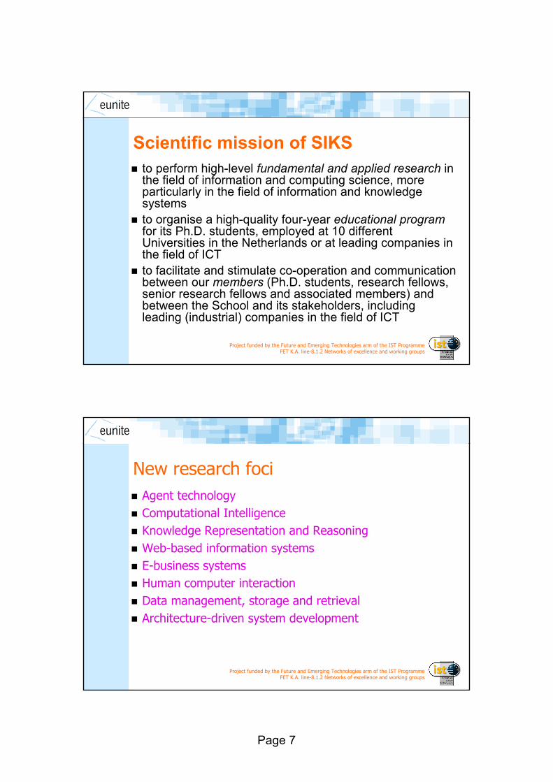
SIKSSIKS is the Dutch Research School for Information and Knowledge systems. It was founded in 1996 by researchers in the field of Artificial Intelligence, Databases & Information Systems and Software Engineering SIKS is an interuniversity research school that comprises 12 research groups in which currently over 270 researchers are active, including 120 Ph.D-studentsIt's Administrative University is the Free University of Amsterdam. The office of SIKS is located at Utrecht University. SIKS received its accreditation by KNAW in 1998In June 2003 SIKS was re-accreditated by KNAW for a period of 6 years.

SIKS is the Dutch Research School for Information and Knowledge systems. It was founded in 1996 by researchers in the field of Artificial Intelligence, Databases & Information Systems and Software Engineering SIKS is an interuniversity research school that comprises 12 research groups in which currently over 270 researchers are active, including 120 Ph.D-studentsIt's Administrative University is the Free University of Amsterdam. The office of SIKS is located at Utrecht University. SIKS received its accreditation by KNAW in 1998In June 2003 SIKS was re-accreditated by KNAW for a period of 6 years.

Page 7



Scientific mission of SIKSto perform high-level fundamental and applied research inthe field of information and computing science, more particularly in the field of information and knowledge systemsto organise a high-quality four-year educational programfor its Ph.D. students, employed at 10 different Universities in the Netherlands or at leading companies in the field of ICT to facilitate and stimulate co-operation and communication between our members (Ph.D. students, research fellows, senior research fellows and associated members) and between the School and its stakeholders, including leading (industrial) companies in the field of ICT

to perform high-level fundamental and applied research inthe field of information and computing science, more particularly in the field of information and knowledge systemsto organise a high-quality four-year educational programfor its Ph.D. students, employed at 10 different Universities in the Netherlands or at leading companies in the field of ICT to facilitate and stimulate co-operation and communication between our members (Ph.D. students, research fellows, senior research fellows and associated members) and between the School and its stakeholders, including leading (industrial) companies in the field of ICT



New research fociAgent technology Computational Intelligence Knowledge Representation and Reasoning Web-based information systems E-business systems Human computer interaction Data management, storage and retrieval Architecture-driven system development

Agent technology Computational Intelligence Knowledge Representation and Reasoning Web-based information systems E-business systems Human computer interaction Data management, storage and retrieval Architecture-driven system development

Page 8



More information on SIKS

Address:

SIKSUtrecht UniversityInstitute for information and computing sciencesP. O. Box 80.0893508 TB Utrecht

Phone: +30-253-4083/1454

Fax: +30-251-3791

Email address: [email protected] site: http://www.siks.nl/

Address:

SIKSUtrecht UniversityInstitute for information and computing sciencesP. O. Box 80.0893508 TB Utrecht

Phone: +30-253-4083/1454

Fax: +30-251-3791

Email address: [email protected] site: http://www.siks.nl/





Page 9



First workshopFinance in generalAmsterdam, 15 November 2002Proceedings on the web

Finance in generalAmsterdam, 15 November 2002Proceedings on the web





Page 10



ProgramShow pdf file…

Focus on Intelligent Risk Analysis & Management– statistical approaches (including the Bayesian approach)– machine learning approach (decision tree)– genetic algorithms – fuzzy logic

Other contributions using techniques from informatics– OLAP– agent-based systems

Show pdf file…

Focus on Intelligent Risk Analysis & Management– statistical approaches (including the Bayesian approach)– machine learning approach (decision tree)– genetic algorithms – fuzzy logic

Other contributions using techniques from informatics– OLAP– agent-based systems

1

Financial Risk Analysis & Management :

An Overview

Winfried G. Hallerbach

EUNITE – May 19, 2004

intelligent risk analysis & management in finance

W.G. Hallerbach 2

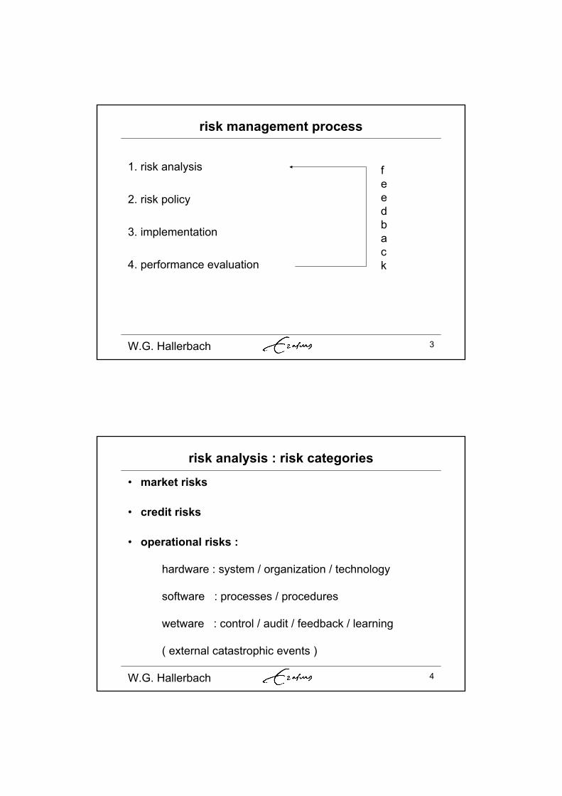
outline

• risk management framework

• model risk

• cognitive biases in DM under uncertainty

• decision context & performance evaluation

2

W.G. Hallerbach 3

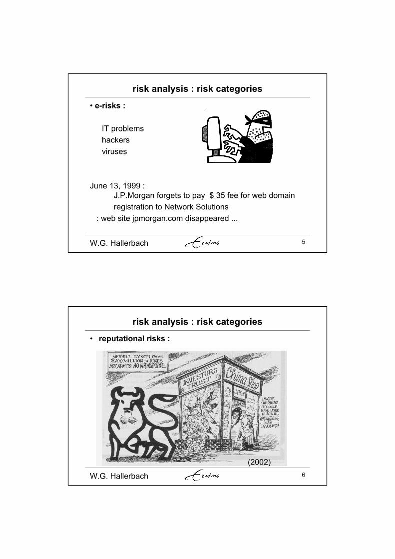
risk management process

1. risk analysis

2. risk policy

3. implementation

4. performance evaluation

feedback

W.G. Hallerbach 4

risk analysis : risk categories

• market risks

• credit risks

• operational risks :

hardware : system / organization / technology

software : processes / procedures

wetware : control / audit / feedback / learning

( external catastrophic events )

3

W.G. Hallerbach 5


• e-risks :

IT problemshackersviruses

June 13, 1999 : J.P.Morgan forgets to pay $ 35 fee for web domainregistration to Network Solutions

: web site jpmorgan.com disappeared ...

W.G. Hallerbach 6


• reputational risks :

(2002)

4

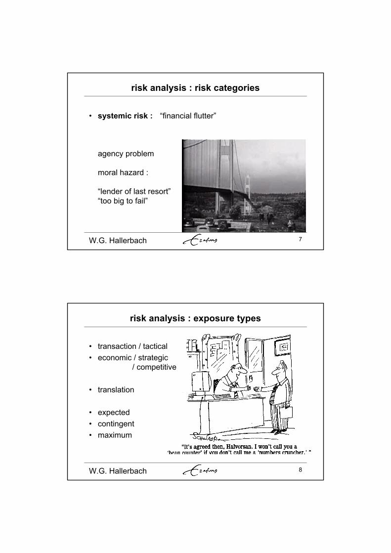
W.G. Hallerbach 7


• systemic risk : “financial flutter”

agency problem

moral hazard :

“lender of last resort”“too big to fail”

W.G. Hallerbach 8

risk analysis : exposure types

• transaction / tactical• economic / strategic

/ competitive

• translation

• expected• contingent• maximum

5

W.G. Hallerbach 9

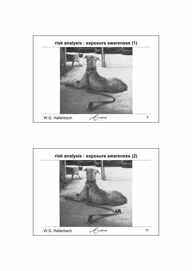
risk analysis : exposure awareness (1)

W.G. Hallerbach 10

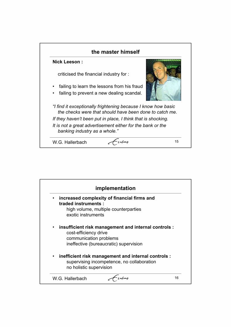
risk analysis : exposure awareness (2)

6

W.G. Hallerbach 11

risk policy

• horizon

• risk – return trade-off :

- RAROC- is risk manager biggest enemy of commercial manager ?

• “economic hedging” vs entrepreneurship

• “views” selective hedging

W.G. Hallerbach 12

diversification

7

W.G. Hallerbach 13

enterprise-wide risk management

macro view :

• netting exposures : ICT challenge

• portfolio effect : econometric challenge

• overall risk-return trade-off

• contribution to RAROC :ex anteex post

W.G. Hallerbach 14

downside & upside

upside potential vs downside risk :in Chinese :

risk :

danger opportunity

• only riskfree rate is riskfree

• profit opportunities are risky ventures

8

W.G. Hallerbach 15

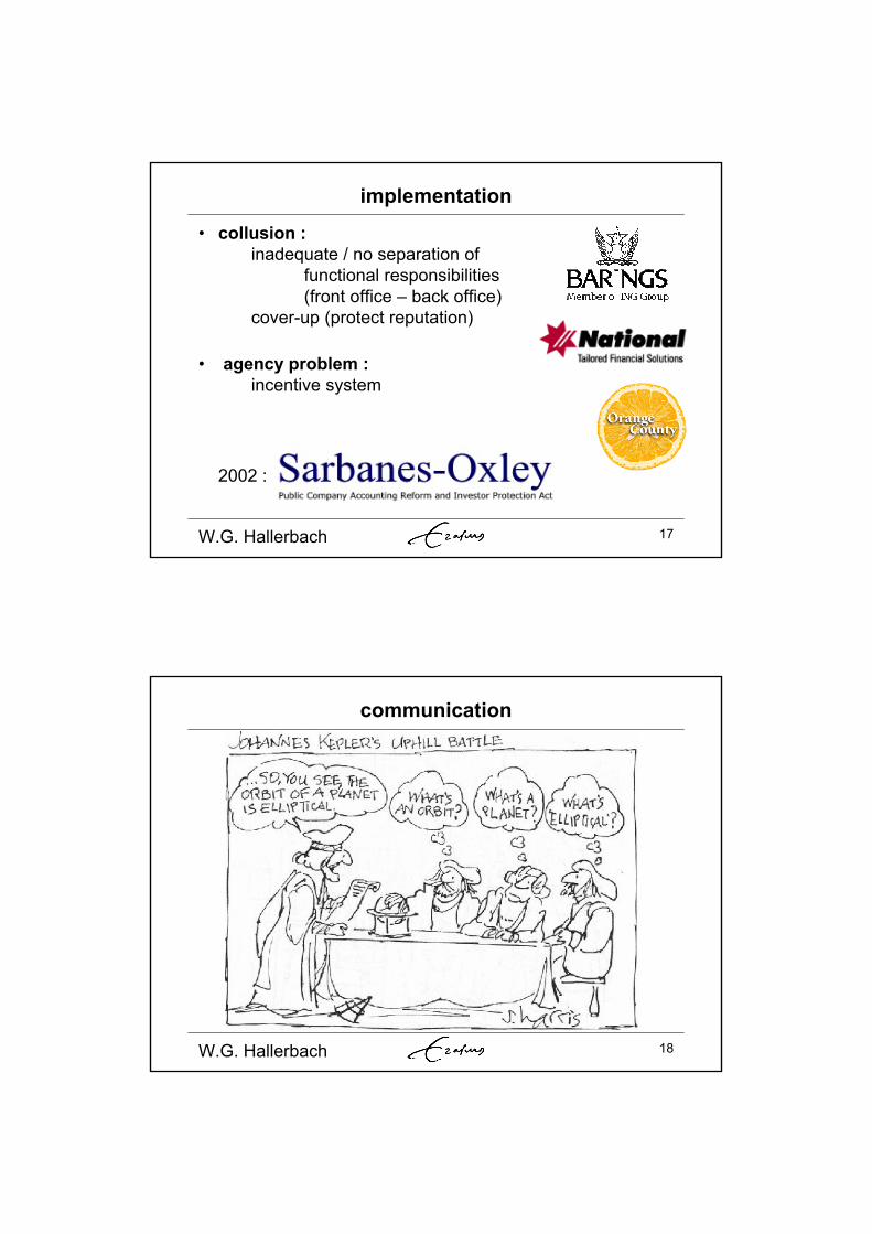
the master himself

Nick Leeson :

criticised the financial industry for :

• failing to learn the lessons from his fraud• failing to prevent a new dealing scandal.

“I find it exceptionally frightening because I know how basic the checks were that should have been done to catch me.

If they haven’t been put in place, I think that is shocking. It is not a great advertisement either for the bank or the

banking industry as a whole.”

W.G. Hallerbach 16

implementation

• increased complexity of financial firms and traded instruments :

high volume, multiple counterpartiesexotic instruments

• insufficient risk management and internal controls :cost-efficiency drivecommunication problemsineffective (bureaucratic) supervision

• inefficient risk management and internal controls :supervising incompetence, no collaborationno holistic supervision

9

W.G. Hallerbach 17

implementation

• collusion :inadequate / no separation of

functional responsibilities (front office – back office)

cover-up (protect reputation)

• agency problem :incentive system

2002 :

W.G. Hallerbach 18

communication

10

W.G. Hallerbach 19

outline


• model risk



W.G. Hallerbach 20

model risk

Emanuel Derman : “In physics, you’re playing against God; in finance, you’re playing against people.”

11

W.G. Hallerbach 21

model risk

models used for : • valuation : “mark-to-model” i.s.o. mark-to-market• risk analysis

model risk :• wrong input data : volatility• wrong parameter estimates• wrong / incomplete model• wrong implementation

garbage in – garbage out (NatWest, UBS)

W.G. Hallerbach 22

low fat modeling

no hairy hypotheses,

but

shave with Occam’s razor :

principle of parsimony

12

W.G. Hallerbach 23

Better roughly right, than exactly wrong

“The mathematics of models may be precise, but the models by definition are not…”

(Robert Merton, 1995)

“… particularly in the field of finance, what is needed are approximate answers to the precise problem rather than precise answers to the approximate problem.

(K.L. Hastie, 1982)

W.G. Hallerbach 24

search for the Holy Scale

• speed versus accuracy • procedure risk (Beder, FAJ

1995)

• estimation risk

13

W.G. Hallerbach 25

stress testing

• no worst case scenarios

• historical scenarios …

• extreme losses not necessarily from extreme factor movements

W.G. Hallerbach 26

outline


• model risk



14

W.G. Hallerbach 27

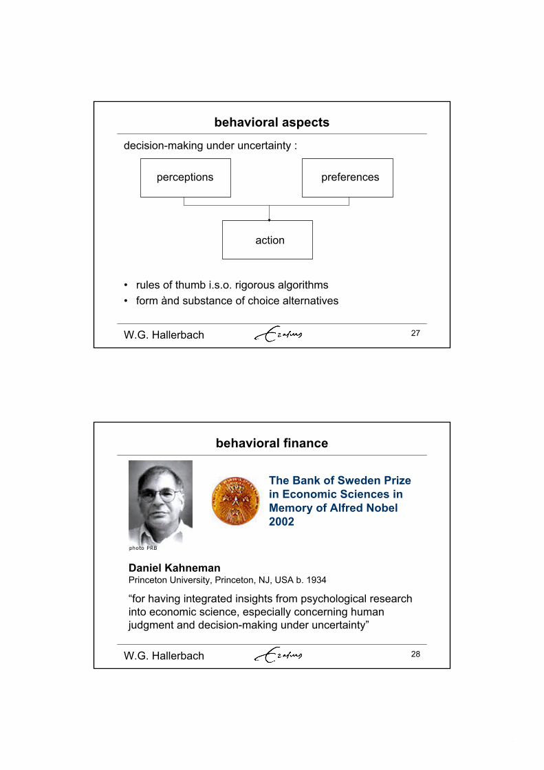
behavioral aspects

decision-making under uncertainty :

perceptions preferences

action

• rules of thumb i.s.o. rigorous algorithms• form ànd substance of choice alternatives

W.G. Hallerbach 28

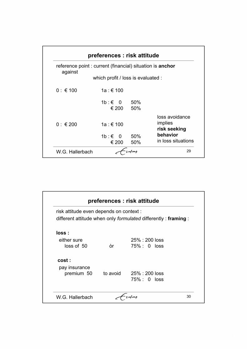
behavioral finance

The Bank of Sweden Prize in Economic Sciences in Memory of Alfred Nobel 2002

Daniel KahnemanPrinceton University, Princeton, NJ, USA b. 1934

“for having integrated insights from psychological research into economic science, especially concerning human judgment and decision-making under uncertainty”

15

W.G. Hallerbach 29

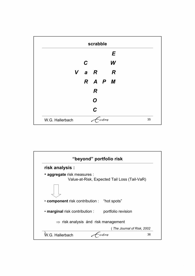
preferences : risk attitude

reference point : current (financial) situation is anchoragainst

which profit / loss is evaluated :

0 : € 100 1a : € 100

1b : € 0 50%€ 200 50%

0 : € 200 1a : € 100

1b : € 0 50%€ 200 50%

loss avoidance implies risk seeking behaviorin loss situations

W.G. Hallerbach 30

preferences : risk attitude

risk attitude even depends on context : different attitude when only formulated differently : framing :

loss :either sure 25% : 200 loss

loss of 50 òr 75% : 0 loss

cost :pay insurance

premium 50 to avoid 25% : 200 loss75% : 0 loss

16

W.G. Hallerbach 31

perceptions : context framing

W.G. Hallerbach 32

the human factor

people :

• have illusions about their chances

• have illusions about their control of thesituation

• are overconfident in their capabilities• tend to do almost everything to avoid losses• neglect to put their decisions in a broader

context (“mental accounting”)

17

W.G. Hallerbach 33

learning

Good judgment comes from experience. Experience comes from bad judgment.

(Walter Wriston, banker)

W.G. Hallerbach 34

outline


• model risk



18

W.G. Hallerbach 35

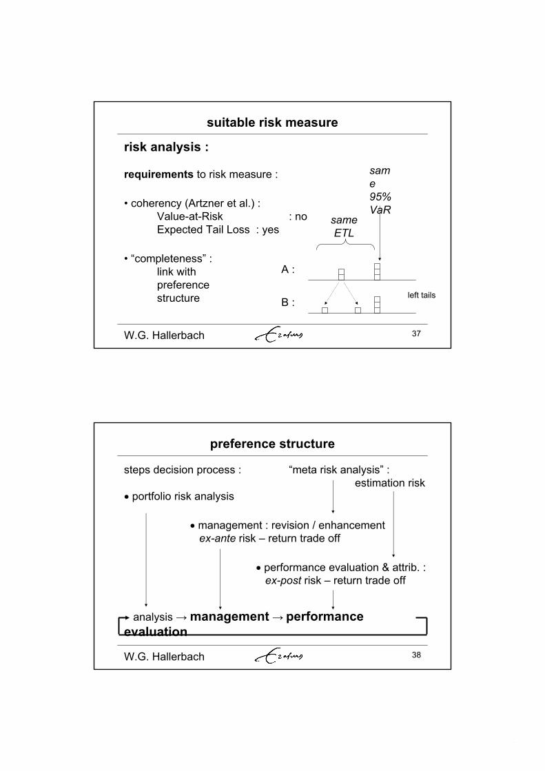
scrabble

EC W

V a R RR A P M

ROC

W.G. Hallerbach 36

“beyond” portfolio risk

risk analysis : • aggregate risk measures :

Value-at-Risk, Expected Tail Loss (Tail-VaR)

• component risk contribution : “hot spots”

• marginal risk contribution : portfolio revision

risk analysis ánd risk management( The Journal of Risk, 2002

)

19

W.G. Hallerbach 37

suitable risk measure

risk analysis :

requirements to risk measure :

• coherency (Artzner et al.) :Value-at-Risk : noExpected Tail Loss : yes

• “completeness” : link with preferencestructure

same95%VaR

sameETL

A :

B :left tails

W.G. Hallerbach 38

preference structure

steps decision process : “meta risk analysis” : estimation risk

portfolio risk analysis

management : revision / enhancementex-ante risk – return trade off

performance evaluation & attrib. :ex-post risk – return trade off

analysis management performance evaluation

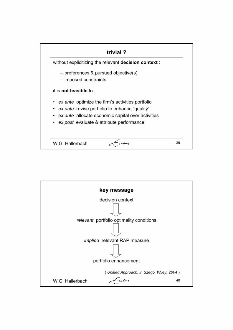
20

W.G. Hallerbach 39

trivial ?

without explicitizing the relevant decision context :

– preferences & pursued objective(s)– imposed constraints

it is not feasible to :

• ex ante optimize the firm’s activities portfolio• ex ante revise portfolio to enhance “quality”• ex ante allocate economic capital over activities • ex post evaluate & attribute performance

W.G. Hallerbach 40

key message

decision context

relevant portfolio optimality conditions

implied relevant RAP measure

portfolio enhancement

( Unified Approach, in Szegö, Wiley, 2004 )

21

W.G. Hallerbach 41

wrapping up …

• do not blindly trust your senses• do not blindly trust models• make sure you fully understand what you’re doing

• risk = unexpected• recognize the power of diversification• acknowledge bounded rationality• beware of cognitive biases

• choose any deck chair on the Titanic …• when you think there’s a fool in the market ….

W.G. Hallerbach 42

www.GARP.com

everything you always wanted to know about VaR but were afraid to ask … :

www.gloriamundi.org

many more useful links : www.finance-on-eur.nl

URLs

Professional Risk Managers’ Int’l Assoc.www.prmia.org

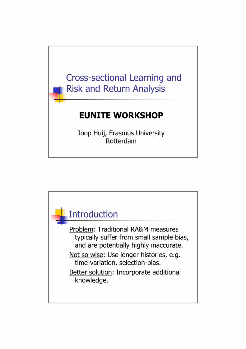
1

Cross-sectional Learning and Risk and Return Analysis

EUNITE WORKSHOP

Joop Huij, Erasmus University Rotterdam

IntroductionProblem: Traditional RA&M measures

typically suffer from small sample bias, and are potentially highly inaccurate.

Not so wise: Use longer histories, e.g. time-variation, selection-bias.

Better solution: Incorporate additional knowledge.

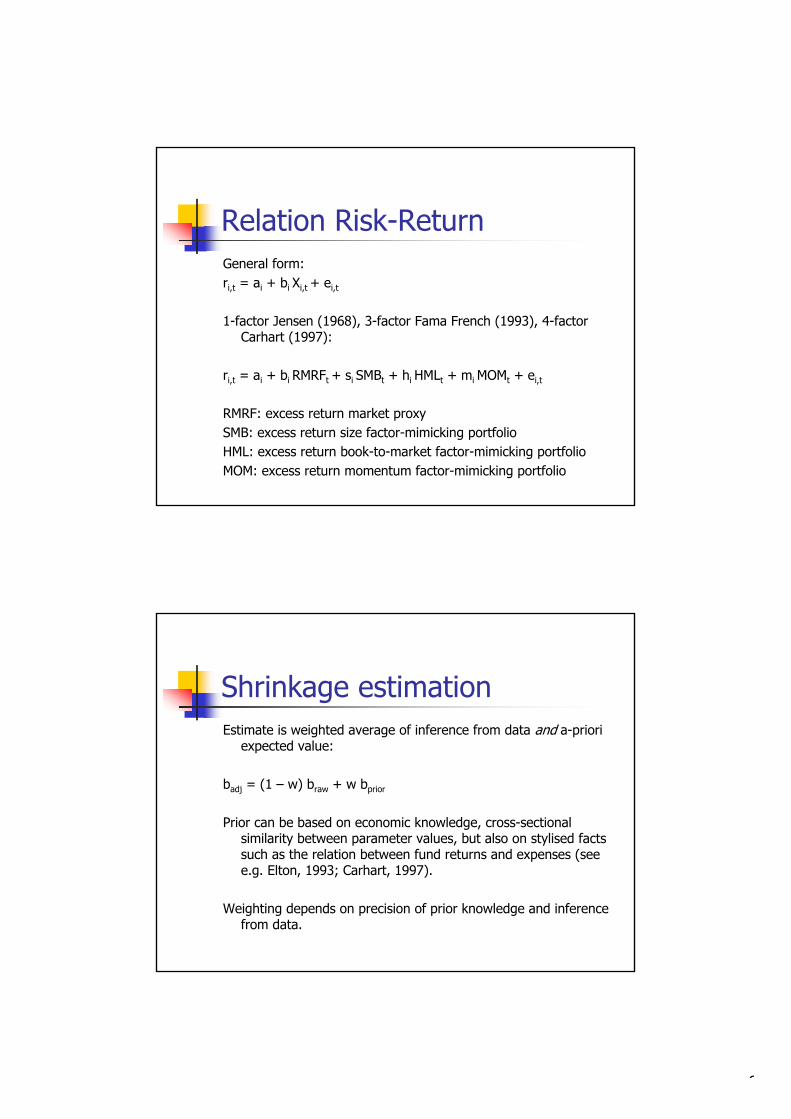
2

Relation Risk-ReturnGeneral form:ri,t = ai + bi Xi,t + ei,t

1-factor Jensen (1968), 3-factor Fama French (1993), 4-factorCarhart (1997):

ri,t = ai + bi RMRFt + si SMBt + hi HMLt + mi MOMt + ei,t

RMRF: excess return market proxySMB: excess return size factor-mimicking portfolioHML: excess return book-to-market factor-mimicking portfolioMOM: excess return momentum factor-mimicking portfolio

Shrinkage estimationEstimate is weighted average of inference from data and a-priori

expected value:

badj = (1 – w) braw + w bprior

Prior can be based on economic knowledge, cross-sectional similarity between parameter values, but also on stylised facts such as the relation between fund returns and expenses (see e.g. Elton, 1993; Carhart, 1997).

Weighting depends on precision of prior knowledge and inference from data.

3

Panel Data (1)Stein rule (Swamy, 1970):

ßshrunk = (1 – c/F) ßols + c/F ßpooled

ßols: individual time series estimateßpooled : pooled estimateC/F: measure for homogeneity; standardized test-statistic to

H0: ß1 = ß2 =…= ßN = ßpooled

Panel Data (2)Chow test:

F = (e’e – e1’e1 – e2’e2 - … - eN’eN)/(N-1)k 1/(e1’e1 – e2’e2 - … - eN’eN)/N(T-k)

Degrees of freedom:

(N-1)k –2 / N(T-k) + 2

Basically, ratio of unxeplained part by pooled regression and individual regressions.

4

Panel Data (3)Bloomberg’s adjusted betas:

Betaadj = 0.7 betaraw + 0.3

Simple or simplified (c/F = 0.3; bpooled = 1)?

Experiment: Perform Chow-test on 5 year return history of 25 randomly chosen mutual funds.

c/F 0.10 Although values differs, underlying idea seems to make sense.

Panel Data (4)Basic characteristics Stein rule estimator:

Exploits cross-sectional similarityLinear adjustment to raw estimatesrmseadj rmseols for all bi

However, relative performance/ risk estimates, i.e. rankings, remain unchanched.

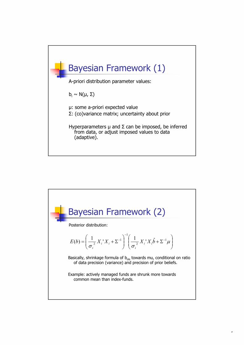
5

Bayesian Framework (1)A-priori distribution parameter values:

bi ~ N(µ, )

µ: some a-priori expected value: (co)variance matrix; uncertainty about prior

Hyperparameters µ and can be imposed, be inferred from data, or adjust imposed values to data (adaptive).

Bayesian Framework (2)Posterior distribution:

12

1

12

ˆ'1'1)( bXXXXbE iii

iii

Basically, shrinkage formula of bols towards mu, conditional on ratio of data precision (variance) and precision of prior beliefs.

Example: actively managed funds are shrunk more towards common mean than index-funds.

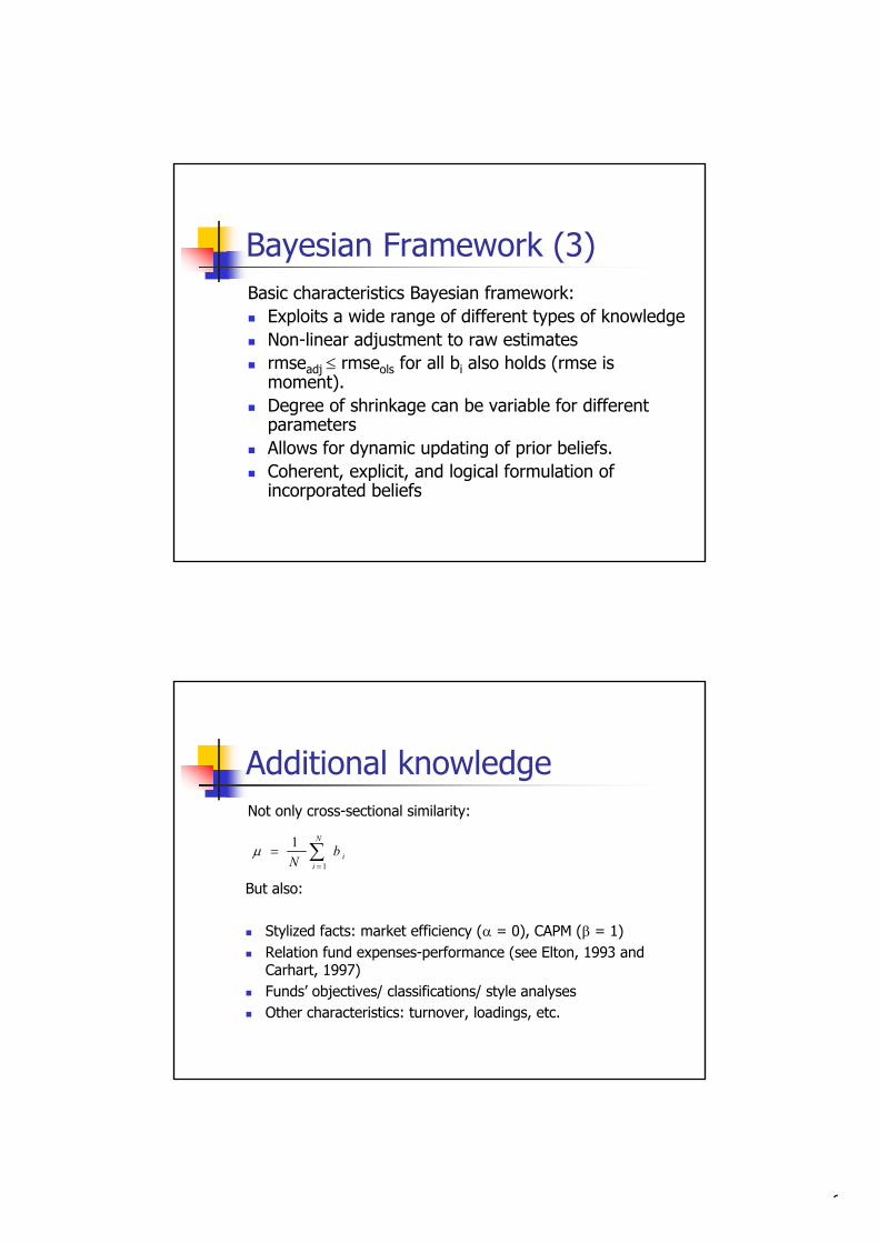
6

Bayesian Framework (3)Basic characteristics Bayesian framework:

Exploits a wide range of different types of knowledgeNon-linear adjustment to raw estimatesrmseadj rmseols for all bi also holds (rmse is moment).Degree of shrinkage can be variable for different parametersAllows for dynamic updating of prior beliefs.Coherent, explicit, and logical formulation of incorporated beliefs

Additional knowledgeNot only cross-sectional similarity:

N

iibN 1

1

But also:

Stylized facts: market efficiency ( = 0), CAPM ( = 1)Relation fund expenses-performance (see Elton, 1993 and Carhart, 1997)Funds’ objectives/ classifications/ style analysesOther characteristics: turnover, loadings, etc.

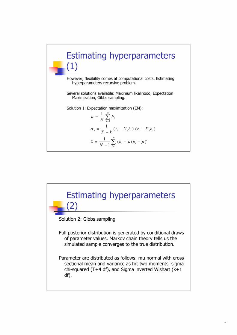
7

Estimating hyperparameters (1)However, flexibility comes at computational costs. Estimating

hyperparameters recursive problem.

Several solutions available: Maximum likelihood, Expectation Maximization, Gibbs sampling.

Solution 1: Expectation maximization (EM):

N

iii

iiiiiii

i

N

ii

bbN

bXrbXrkT

bN

1

1

)'((1

1

)()'(1

1

Estimating hyperparameters (2)

Solution 2: Gibbs sampling

Full posterior distribution is generated by conditional draws of parameter values. Markov chain theory tells us the simulated sample converges to the true distribution.

Parameter are distributed as follows: mu normal with cross-sectional mean and variance as firt two moments, sigmaichi-squared (T+4 df), and Sigma inverted Wishart (k+1 df).

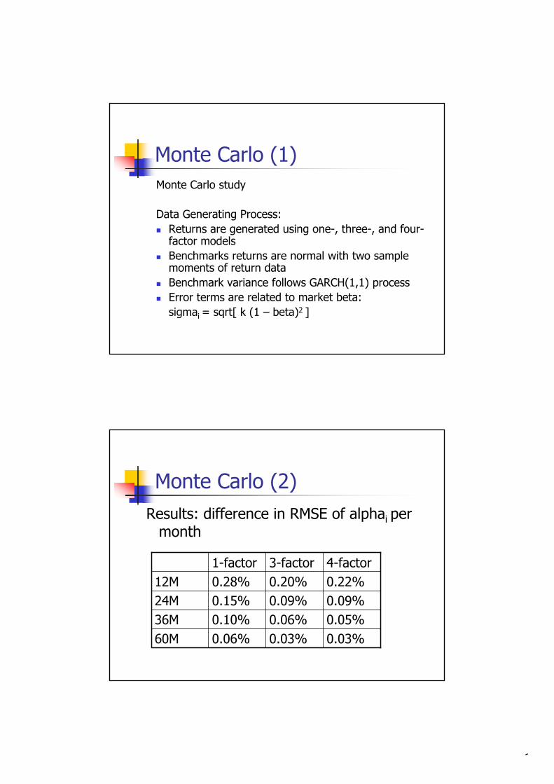
8

Monte Carlo (1)Monte Carlo study

Data Generating Process:Returns are generated using one-, three-, and four-factor modelsBenchmarks returns are normal with two sample moments of return dataBenchmark variance follows GARCH(1,1) processError terms are related to market beta:sigmai = sqrt[ k (1 – beta)2 ]

Monte Carlo (2)Results: difference in RMSE of alphai per

month

0.05%0.06%0.10%36M0.03%0.03%0.06%60M

0.09%0.09%0.15%24M0.22%0.20%0.28%12M4-factor3-factor1-factor

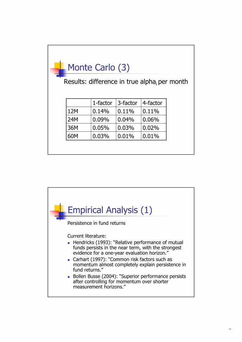
9

Monte Carlo (3)Results: difference in true alphai per month

0.02%0.03%0.05%36M0.01%0.01%0.03%60M

0.06%0.04%0.09%24M0.11%0.11%0.14%12M4-factor3-factor1-factor

Empirical Analysis (1)Persistence in fund returns

Current literature:Hendricks (1993): “Relative performance of mutual funds persists in the near term, with the strongest evidence for a one-year evaluation horizon.”Carhart (1997): “Common risk factors such as momentum almost completely explain persistence in fund returns.”Bollen Busse (2004): “Superior performance persists after controlling for momentum over shorter measurement horizons.”

10

Empirical Analysis (2)Typical setup to test for persistence:

1. Estimate abnormal performance (alpha) for all funds.

2. Rank funds based on alpha3. Evaluate subsequent performance4. Analyze correlation between alpha and

subsequent performance

Empirical Analysis (3)CRSP survivorship free mutual fund database

Features:Dates back to 1962Over 23,000 mutual fundsIncludes all existing fundsMonthly frequencies

Sample: 7,669 US equity funds, 1985-2003

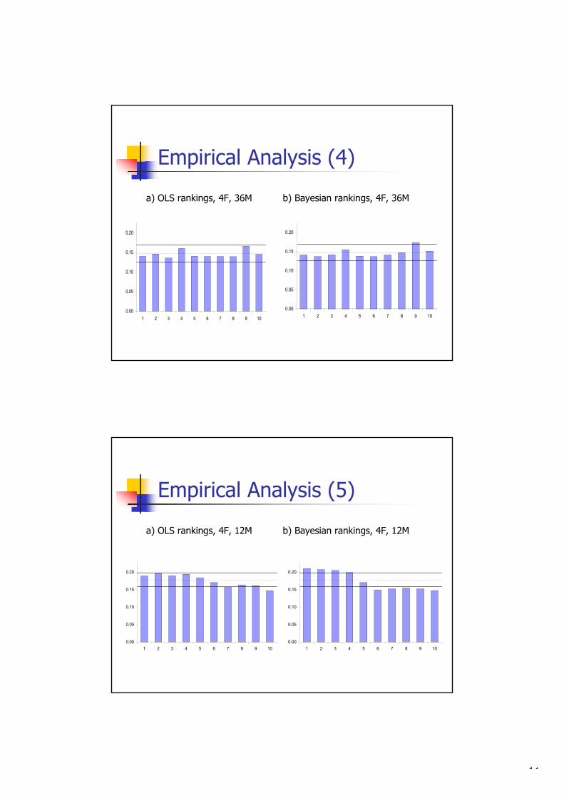
11

Empirical Analysis (4)

0.00

0.05

0.10

0.15

0.20

1 2 3 4 5 6 7 8 9 10

0.00

0.05

0.10

0.15

0.20

1 2 3 4 5 6 7 8 9 10

a) OLS rankings, 4F, 36M b) Bayesian rankings, 4F, 36M


0.00

0.05

0.10

0.15

0.20

1 2 3 4 5 6 7 8 9 100.00

0.05

0.10

0.15

0.20

1 2 3 4 5 6 7 8 9 10

a) OLS rankings, 4F, 12M b) Bayesian rankings, 4F, 12M

12

Empirical Analysis (6)Robustness of results:

Alternative test 1: Fama MacBeth regression (1973):

Sharpei,t = a + b alphai,t-1 + ei,t

Positive slope indicates relation between alphai,t-1 and Sharpei,t.

E(bols ) = 0.07 (t-stat: 2.01)

E(bbayes ) = 0.10 (t-stat: 2.35) consistent with previous results

Empirical Analysis (7)Robustness of results:

Alternative test 2: Spearmann rank correlation coefficient:

rphot = 1 – 6 * sumsq(rankingt – rankingt-1) / (N3 – N)

Approximation to the exact correlation.

rpho(bols ) = 0.13 (t-stat: 3.99)

rpho(bbayes ) = 0.16 (t-stat: 4.14) consistent with previous results

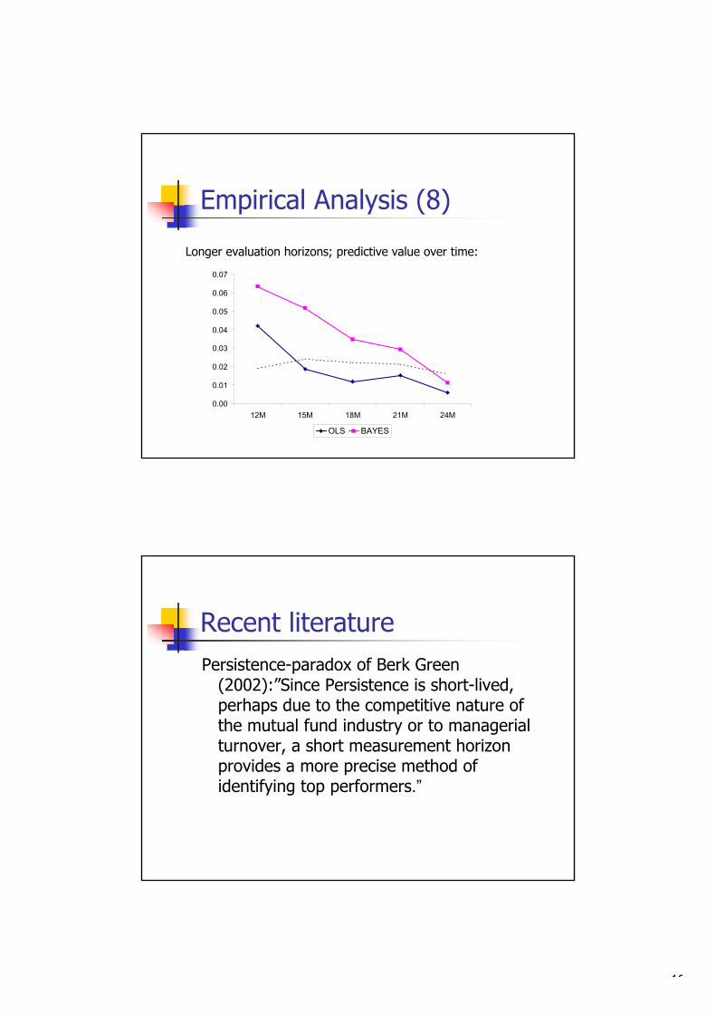
13


0.00

0.01

0.02

0.03

0.04

0.05

0.06

0.07

12M 15M 18M 21M 24M

OLS BAYES

Longer evaluation horizons; predictive value over time:

Recent literaturePersistence-paradox of Berk Green

(2002):”Since Persistence is short-lived, perhaps due to the competitive nature of the mutual fund industry or to managerial turnover, a short measurement horizon provides a more precise method of identifying top performers.”

14

ImplicationsCommercial information services like

Morningstar provide fund ratings typically based on three to five years of return history.

Our results indicate that such long ranking period do not provide relevant information about future performance.

1

1

Market timing:A decomposition of mutual fund returns

Pieter Jelle van der SluisVrije Universiteit & ABP Investments

[email protected]

Jointly with Laurens Swinkels (Robeco) and Marno Verbeek (EUR)

Smart Adaptive Systems in FinanceErasmus University, May 19, 2004

2

The views expressed in this paper are those ofthe authors and do not necessarily reflect those of their employer and colleagues

2

3

Overview of presentation

Introduction and motivation

• Why explaining dispersion in mutual fund returns

Contributions• Decomposition of fund return• Dynamic asset allocation model• Performance related to trading activity and expense ratio

Conclusions

4

Introduction and motivation

Why invest in mutual funds?

Managers choose• the right stocks (selection skill)• or hold cash if the stock market is ‘overvalued’ (timing skill)

Focus of our paper: asset allocation funds

Dispersion of returns and variance of mutual funds• Why? Explanation why fund returns are different• Attribution of returns to selectivity and timing skill

Should investors care about fund turnover and/or expense ratios?

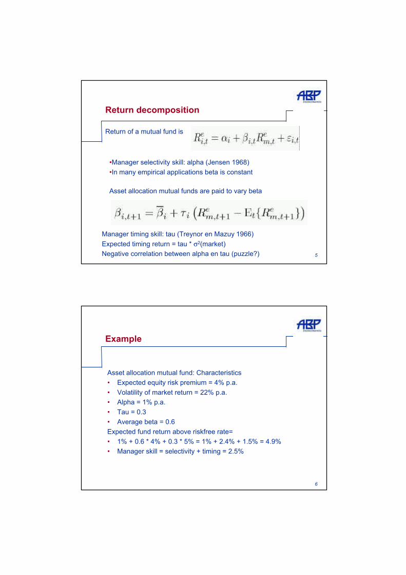
3

5

Return decomposition

Return of a mutual fund is

•Manager selectivity skill: alpha (Jensen 1968)•In many empirical applications beta is constant

Manager timing skill: tau (Treynor en Mazuy 1966) Expected timing return = tau * σ2(market) Negative correlation between alpha en tau (puzzle?)

Asset allocation mutual funds are paid to vary beta

6

Example

Asset allocation mutual fund: Characteristics• Expected equity risk premium = 4% p.a.• Volatility of market return = 22% p.a.• Alpha = 1% p.a.• Tau = 0.3• Average beta = 0.6Expected fund return above riskfree rate=• 1% + 0.6 * 4% + 0.3 * 5% = 1% + 2.4% + 1.5% = 4.9%• Manager skill = selectivity + timing = 2.5%

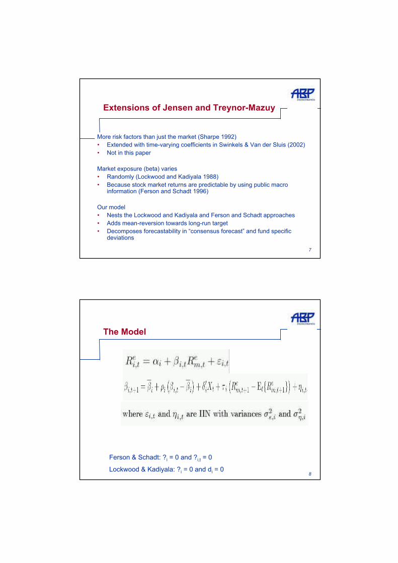
4

7

Extensions of Jensen and Treynor-Mazuy

More risk factors than just the market (Sharpe 1992)• Extended with time-varying coefficients in Swinkels & Van der Sluis (2002)• Not in this paper

Market exposure (beta) varies• Randomly (Lockwood and Kadiyala 1988)• Because stock market returns are predictable by using public macro

information (Ferson and Schadt 1996)

Our model • Nests the Lockwood and Kadiyala and Ferson and Schadt approaches• Adds mean-reversion towards long-run target• Decomposes forecastability in “consensus forecast” and fund specific

deviations

8

The Model

Ferson & Schadt: ?i = 0 and ?i,t = 0

Lockwood & Kadiyala: ?i = 0 and di = 0

5

9

Interpretation of the model

Beta measures sensitivity of the fund to stock market

Alpha is conditional expectation of unexplained part of return

10

Interpretation of the model

Expected return conditional on public information :

Second term r.h.s.

Third term r.h.s.

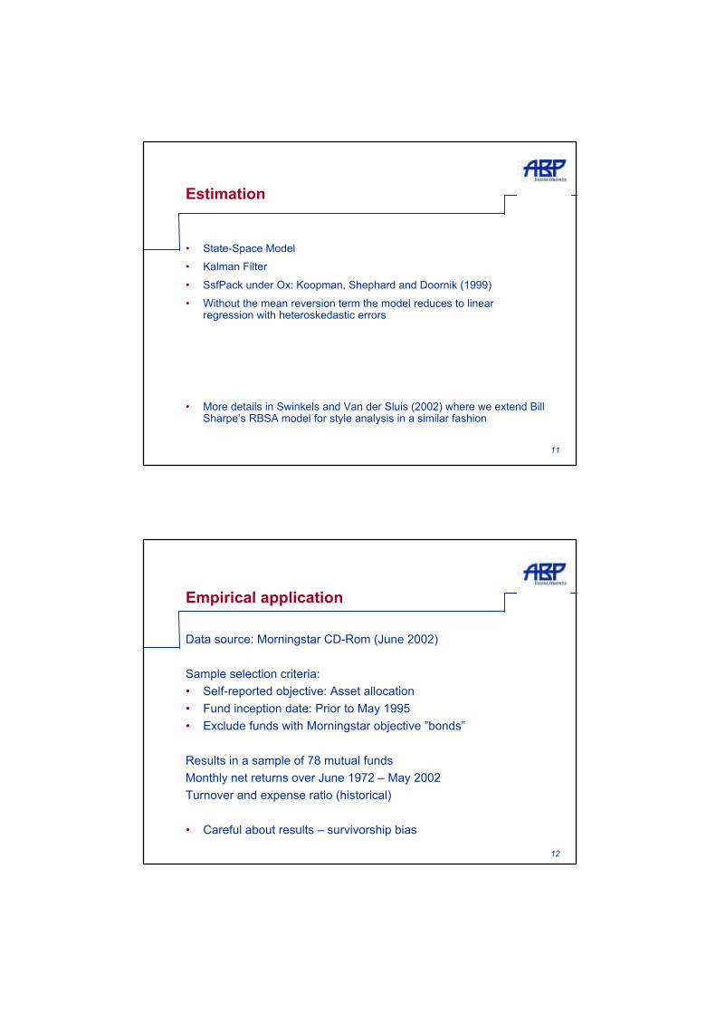
6

11

Estimation

• State-Space Model• Kalman Filter• SsfPack under Ox: Koopman, Shephard and Doornik (1999)• Without the mean reversion term the model reduces to linear

regression with heteroskedastic errors

• More details in Swinkels and Van der Sluis (2002) where we extend Bill Sharpe’s RBSA model for style analysis in a similar fashion

12

Empirical application

Data source: Morningstar CD-Rom (June 2002)

Sample selection criteria:• Self-reported objective: Asset allocation• Fund inception date: Prior to May 1995• Exclude funds with Morningstar objective ”bonds”

Results in a sample of 78 mutual funds Monthly net returns over June 1972 – May 2002Turnover and expense ratio (historical)

• Careful about results – survivorship bias

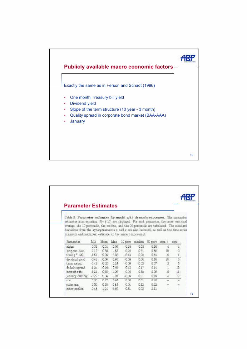
7

13

Publicly available macro economic factors

Exactly the same as in Ferson and Schadt (1996)

• One month Treasury bill yield• Dividend yield• Slope of the term structure (10 year - 3 month)• Quality spread in corporate bond market (BAA-AAA)• January

14

Parameter Estimates

8

15

Boxplots Parameter Estimates Decomposition of mutual fund returns

-0.3

-0.2

-0.1

0

0.1

0.2

0.3

0.4

0.5

0.6

alpha bstar bbar timing economic eta epsilon

10-perc median 90-perc

16

Manager skills: selectivity and timing

9

17

Manager selectivityHistogram of selectivity skill (alpha)

0

5

10

15

20

25

Freq. 2 5 20 20 17 7 2 2 1 2

< -0.30 < -0.20 < -0.10 < 0.00 < 0.10 < 0.20 < 0.30 < 0.40 < 0.50 > 0.50

18

Manager expert timingHistogram of timing skill (tau)

0

5

10

15

20

25

30

Freq. 4 2 4 3 18 24 10 6 4 3

< -0.8% < -0.6% < -0.4% < -0.2% < 0.0% < 0.2% < 0.4% < 0.6% < 0.8% > 0.8%

10

19

Findings Manager Skill

•Correlation between selectivity and timing –0.7

•Size of spread in total manager skill 29bp

•Spread in alpha 35bp

•Spread in timing return 21bp

•Private investors cannot exploit both selectivity and timing at the sametime

20

Non-skill components of conditional expected return

11

21

Long term market exposure

Histogram of longrun target market exposure

0

2

4

6

8

10

12

14

16

18

Freq. 0 0 3 7 5 8 14 17 14 2 4 4

< 0.0 < 0.1 < 0.2 < 0.3 < 0.4 < 0.5 < 0.6 < 0.7 < 0.8 < 0.9 < 1.0 > 1.0

22

Returns from economic exposures

Histogram of average monthly fund returns from economic exposures

0

5

10

15

20

25

30

35

40

Freq. 0 7 14 35 16 3 2 1

< -0.10 < -0.05 < 0.00 < 0.05 < 0.10 < 0.15 < 0.20 > 0.20

12

23

Findings long term and exposures andmean reversion

Median fund long term market exposure 0.61

Mean reversion coefficient is low for most funds somost funds adapt quickly

8 funds have relatively high coefficients

As expected total effect is virtually zero

24

Findings Economic Exposures

•di represent the macro sensitivities that are not explained by expert timing behaviour

•These are macro economic exposures deviating from optimal macro exposure for timing

• About 75% achieves positive return from this component:managers are able to increase fund returns by using economic information and deviating from the public forecast

•Average contribution 2.8bp per month

•Results indicate that mutual fund managers are able to use economic information to increase returns above the public forecast

13

25

Time series variability in market exposures

26

Random exposure shock

For the median fund s ?=0.12

These random changes increase the variance of the conditional return with ( )2,

2 etmRησ

Residual variance of the fund return ( ) 22,

2εη σσ +e

tmRFor the median fund s e=0.92

In contrast to equity mutuals funds, asset allocators appear not to be fully diversified

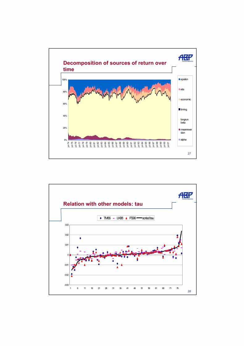
14

27

Decomposition of sources of return over time

0%

20%

40%

60%

80%

100%

jul-7

4ju

l-75

jul-7

6ju

l-77

jul-7

8ju

l-79

jul-8

0ju

l-81

jul-8

2ju

l-83

jul-8

4ju

l-85

jul-8

6ju

l-87

jul-8

8ju

l-89

jul-9

0ju

l-91

jul-9

2ju

l-93

jul-9

4ju

l-95

jul-9

6ju

l-97

jul-9

8ju

l-99

jul-0

0ju

l-01

epsilon

eta

economic

timing

longrunbeta

meanreversion

alpha

28

Relation with other models: tau

-0.03

-0.02

-0.01

0

0.01

0.02

0.03

1 6 11 16 21 26 31 36 41 46 51 56 61 66 71 76

TM66 LK88 FS96 sortedtau

15

29

Relation to other models: alpha

-0.800

-0.400

0.000

0.400

0.800

1.200

1 6 11 16 21 26 31 36 41 46 51 56 61 66 71 76

TM66 LK88 FS96 sorted alpha

30

Turnover and Expense ratios

-0.261.1588Middle 20%

-0.431.1770Middle 20%

0.031.1791Average

0.700.3741Lowest 10%

Expense ratio0.721.25247Highest 10%

1.042.0599Highest 10%

0.350.8519Lowest 10%

Turnover

SkillExpenseTurnover

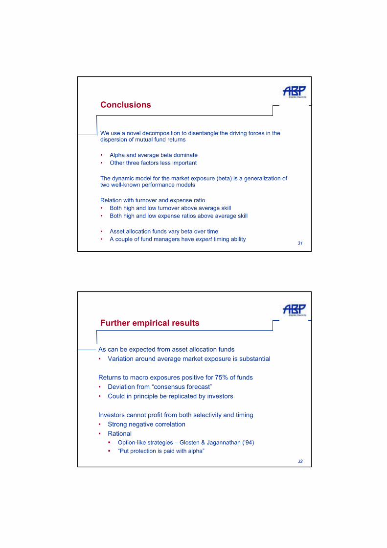
16

31

Conclusions

We use a novel decomposition to disentangle the driving forces in the dispersion of mutual fund returns

• Alpha and average beta dominate• Other three factors less important

The dynamic model for the market exposure (beta) is a generalization of two well-known performance models

Relation with turnover and expense ratio• Both high and low turnover above average skill• Both high and low expense ratios above average skill

• Asset allocation funds vary beta over time• A couple of fund managers have expert timing ability

32

Further empirical results

As can be expected from asset allocation funds• Variation around average market exposure is substantial

Returns to macro exposures positive for 75% of funds• Deviation from “consensus forecast”• Could in principle be replicated by investors

Investors cannot profit from both selectivity and timing• Strong negative correlation• Rational

Option-like strategies – Glosten & Jagannathan (’94)“Put protection is paid with alpha”

1

ROBECO Case


Heru Sataputera Na

I&E Master student Erasmus University Rotterdam

Master Project

Team:Chi Lok CheungHeru Sataputera Na

Supervisor: Jan van den Berg

2

Agenda

IntroductionProblemMain Goals of ResearchApproachImplementation & ResultsConclusion & Future ResearchDiscussion

IntroductionInvesting is Robeco’s core activityPortfolio: Equity and Fixed IncomeStandard Portfolio: customer given proportionStandard ReturnExcess Return = ReturnEQ - ReturnFI

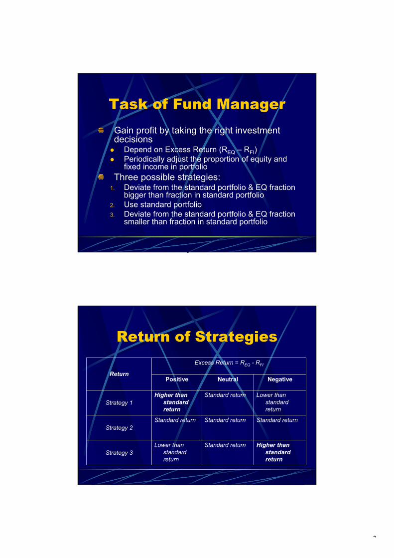
3

Task of Fund ManagerGain profit by taking the right investment decisions

Depend on Excess Return (REQ – RFI)Periodically adjust the proportion of equity and fixed income in portfolio

Three possible strategies:1. Deviate from the standard portfolio & EQ fraction

bigger than fraction in standard portfolio2. Use standard portfolio3. Deviate from the standard portfolio & EQ fraction

smaller than fraction in standard portfolio

Return of Strategies

Higher than standard return

Standard returnLower than standardreturn

Strategy 3

Standard returnStandard returnStandard returnStrategy 2

Lower than standardreturn

Standard returnHigher than standard return

Strategy 1

NegativeNeutralPositive

Excess Return = REQ - RFI

Return

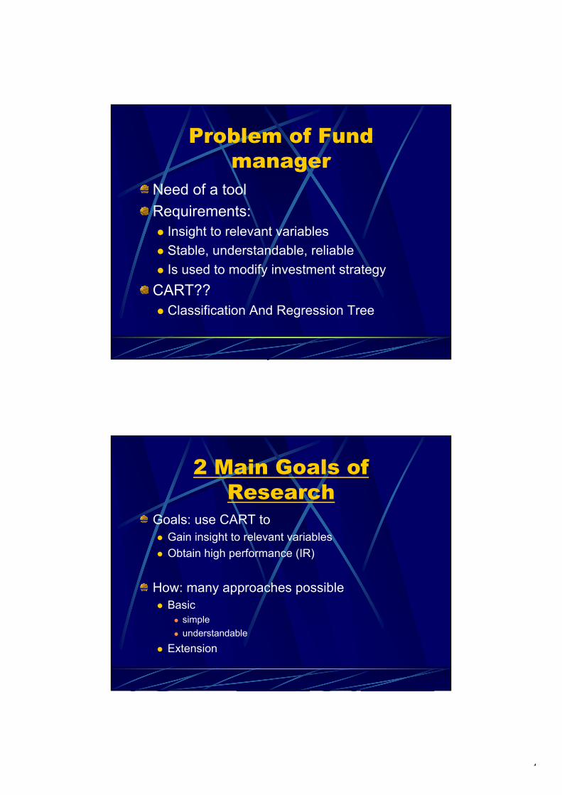
4

Problem of Fund manager

Need of a toolRequirements:

Insight to relevant variablesStable, understandable, reliableIs used to modify investment strategy

CART??Classification And Regression Tree

2 Main Goals of Research

Goals: use CART toGain insight to relevant variablesObtain high performance (IR)

How: many approaches possibleBasic

simpleunderstandable

Extension

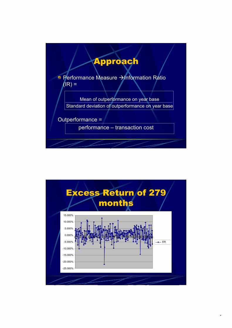
5

Approach

Performance Measure Information Ratio (IR) =

Mean of outperformance on year baseStandard deviation of outperformance on year base

Outperformance =performance – transaction cost

Excess Return of 279 months

-25.000%

-20.000%

-15.000%

-10.000%

-5.000%

0.000%

5.000%

10.000%

15.000%

1 18 35 52 69 86 103 120 137 154 171 188 205 222 239 256273

ER

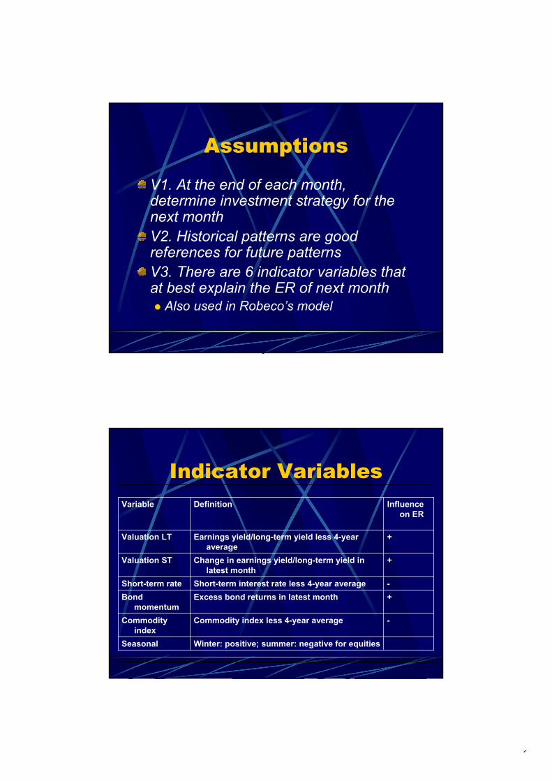
6

Assumptions

V1. At the end of each month, determine investment strategy for the next monthV2. Historical patterns are good references for future patternsV3. There are 6 indicator variables that at best explain the ER of next month

Also used in Robeco’s model

Indicator Variables

Winter: positive; summer: negative for equitiesSeasonal

-Commodity index less 4-year averageCommodity index

+Excess bond returns in latest monthBondmomentum

-Short-term interest rate less 4-year averageShort-term rate

+Change in earnings yield/long-term yield in latest month

Valuation ST

+Earnings yield/long-term yield less 4-year average

Valuation LT

Influence on ER

DefinitionVariable

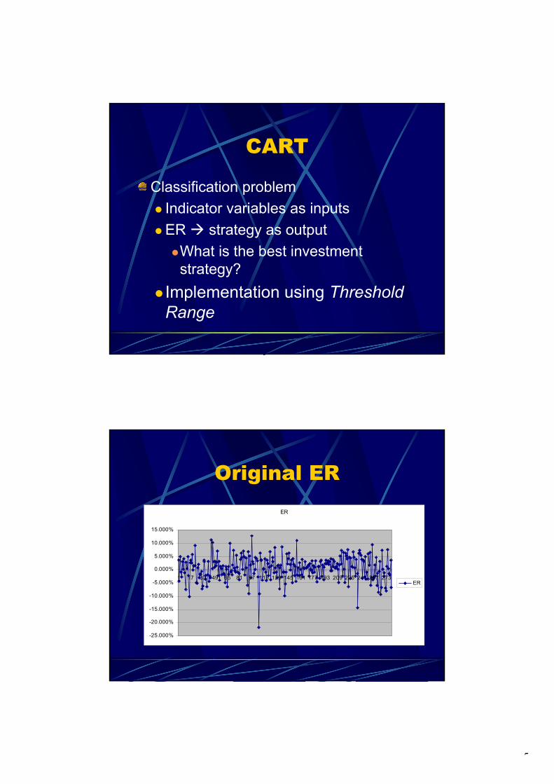
7

CART

Classification problemIndicator variables as inputsER strategy as output

What is the best investment strategy?

Implementation using ThresholdRange

Original ERER

-25.000%

-20.000%

-15.000%

-10.000%

-5.000%

0.000%

5.000%

10.000%

15.000%

1 17 33 49 65 81 97 113 129 145 161 177 193 209 225 241 257 273ER

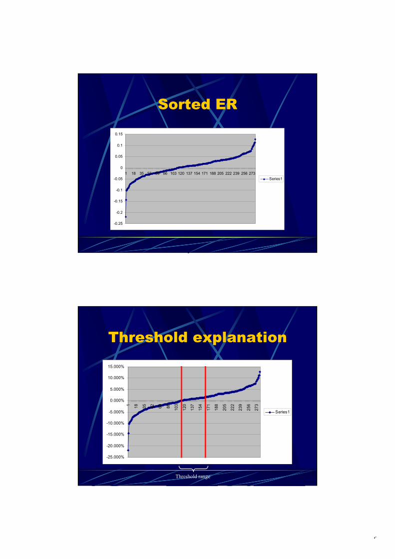
8

Sorted ER

-0.25

-0.2

-0.15

-0.1

-0.05

0

0.05

0.1

0.15

1 18 35 52 69 86 103 120 137 154 171 188 205 222 239 256 273Series1

Threshold explanation

-25.000%

-20.000%

-15.000%

-10.000%

-5.000%

0.000%

5.000%

10.000%

15.000%

1 18 35 52 69 86 103

120

137

154

171

188

205

222

239

256

273

Series1

Threshold range

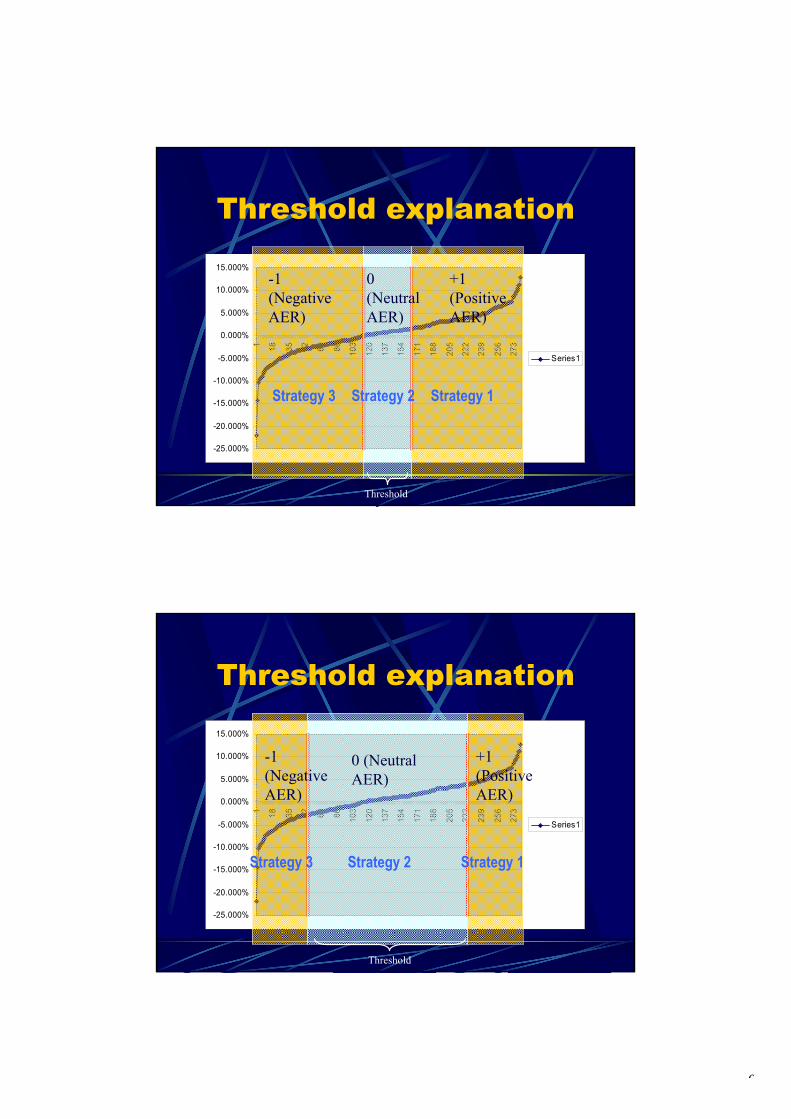
9


-25.000%

-20.000%

-15.000%

-10.000%

-5.000%

0.000%

5.000%

10.000%

15.000%1 18 35 52 69 86 103

120

137

154

171

188

205

222

239

256

273

Series1

Threshold

-1(Negative AER)

+1(Positive AER)

0(NeutralAER)

Strategy 3 Strategy 2 Strategy 1


-25.000%

-20.000%

-15.000%

-10.000%

-5.000%

0.000%

5.000%

10.000%

15.000%

1 18 35 52 69 86 103

120

137

154

171

188

205

222

239

256

273

Series1

Threshold

-1(Negative AER)

+1(Positive AER)

0 (Neutral AER)

Strategy 3 Strategy 2 Strategy 1

10

CART

Input : 6 indicator variablesOutput : AER-class value (-1,0,+1)V4. Fourth Assumption:

Given the input variables, CART can classify the output correctly in most cases

Important Remark

Low error rate high IRLow error rate AER correctly classified in most casesBest threshold high IR

How often deviate from standard portfolio?

What is the best THRESHOLD?Not really trainable with CARTNot a classic CART problem

11

Two steps approach

For each threshold range, generate CART to predict AER

Result: CART with the lowest error rate

Which threshold range provides the highest IR?

Result: BEST threshold range

DATADataset (279 instances)

6 indicator variables + Excess Return (ER)

Train set (219 instances)Output class: on the basis of threshold, ER AERPruning (minimize error rate and tree-complexity)Determine best threshold (using tree) based on IR

Test set (60 instances)Comparison with the ARA model (not done in this research)

12

Input & Output Variables

DiscreteWinter: positive; summer: negative for equities

F

DiscreteAER (OUTPUT)G

ContinueCommodity index less 4-year averageEContinueExcess bond returns in latest monthDContinueShort-term interest rate less 4-year averageC

ContinueChange in earnings yield/long-term yield in latest month

B

ContinueEarnings yield/long-term yield less 4-year average

A

ValueDefinitionVariable

Implementation & Results

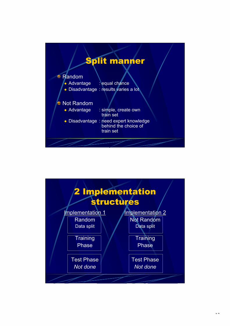
13

Split mannerRandom

Advantage : equal chanceDisadvantage : results varies a lot

Not RandomAdvantage : simple, create own

train set Disadvantage : need expert knowledge

behind the choice of train set

2 Implementation structures

Implementation 1RandomData split

TrainingPhase

Test PhaseNot done

Implementation 2Not Random

Data split

TrainingPhase

Test PhaseNot done

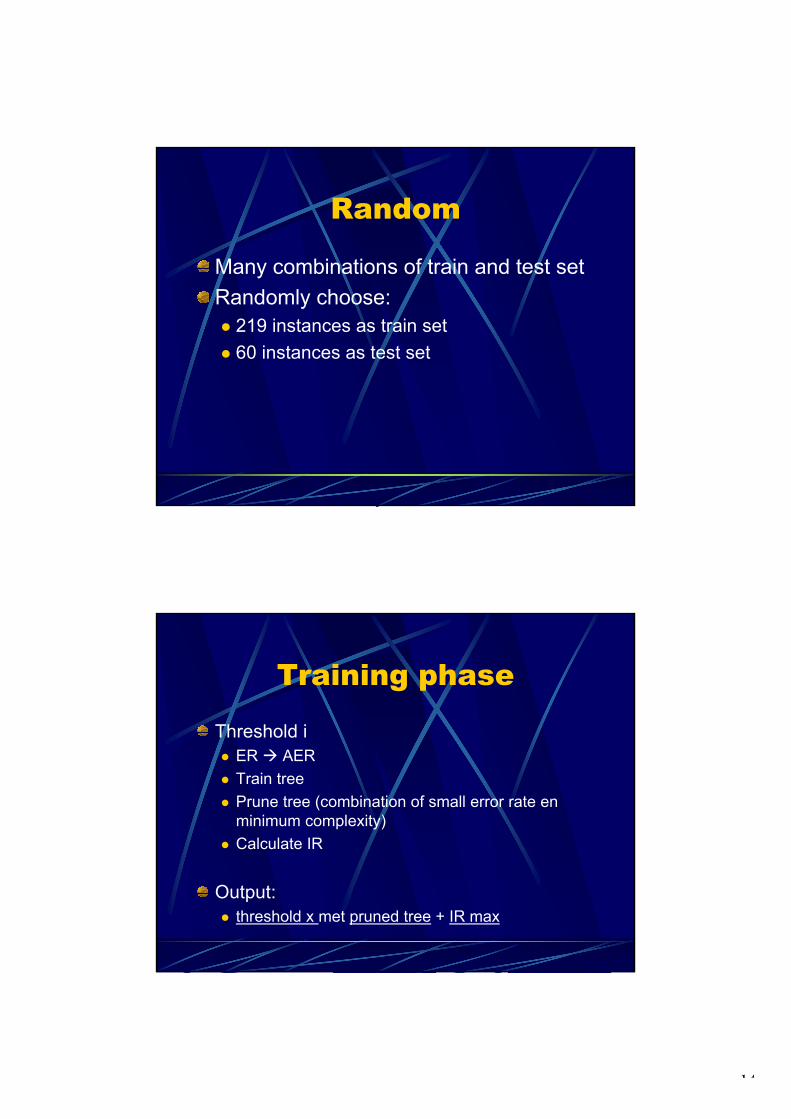
14

Random

Many combinations of train and test setRandomly choose:

219 instances as train set60 instances as test set

Training phase

Threshold iER AERTrain treePrune tree (combination of small error rate en minimum complexity)Calculate IR

Output:threshold x met pruned tree + IR max

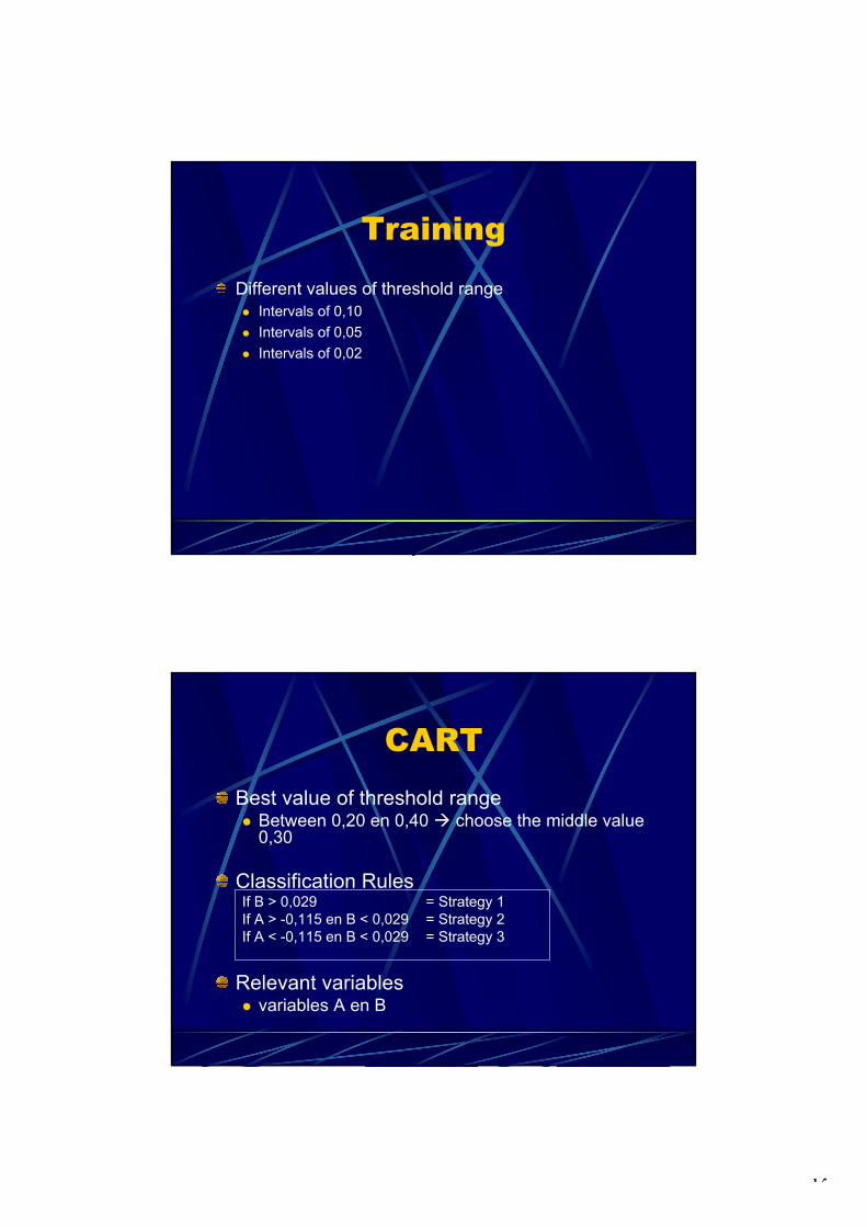
15

TrainingDifferent values of threshold range

Intervals of 0,10 Intervals of 0,05 Intervals of 0,02

CARTBest value of threshold range

Between 0,20 en 0,40 choose the middle value 0,30

Classification RulesIf B > 0,029 = Strategy 1If A > -0,115 en B < 0,029 = Strategy 2If A < -0,115 en B < 0,029 = Strategy 3

Relevant variablesvariables A en B

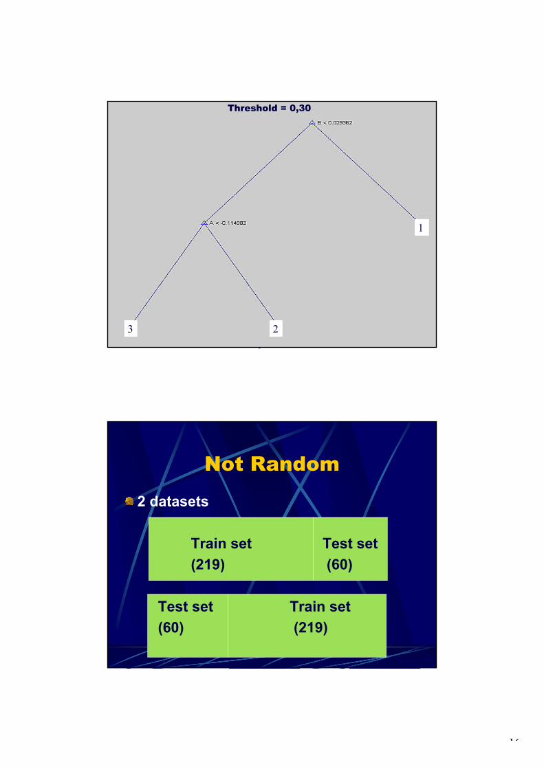
16

Threshold = 0,30

3 2

1

Not Random

2 datasets

Train set Test set(219) (60)

Test set Train set(60) (219)

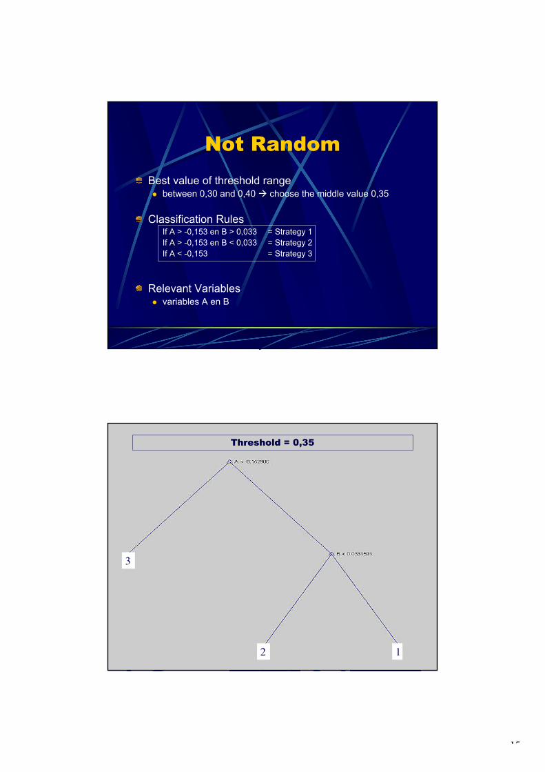
17

Not RandomBest value of threshold range

between 0,30 and 0,40 choose the middle value 0,35

Classification RulesIf A > -0,153 en B > 0,033 = Strategy 1If A > -0,153 en B < 0,033 = Strategy 2If A < -0,153 = Strategy 3

Relevant Variablesvariables A en B

Threshold = 0,35

3

2 1

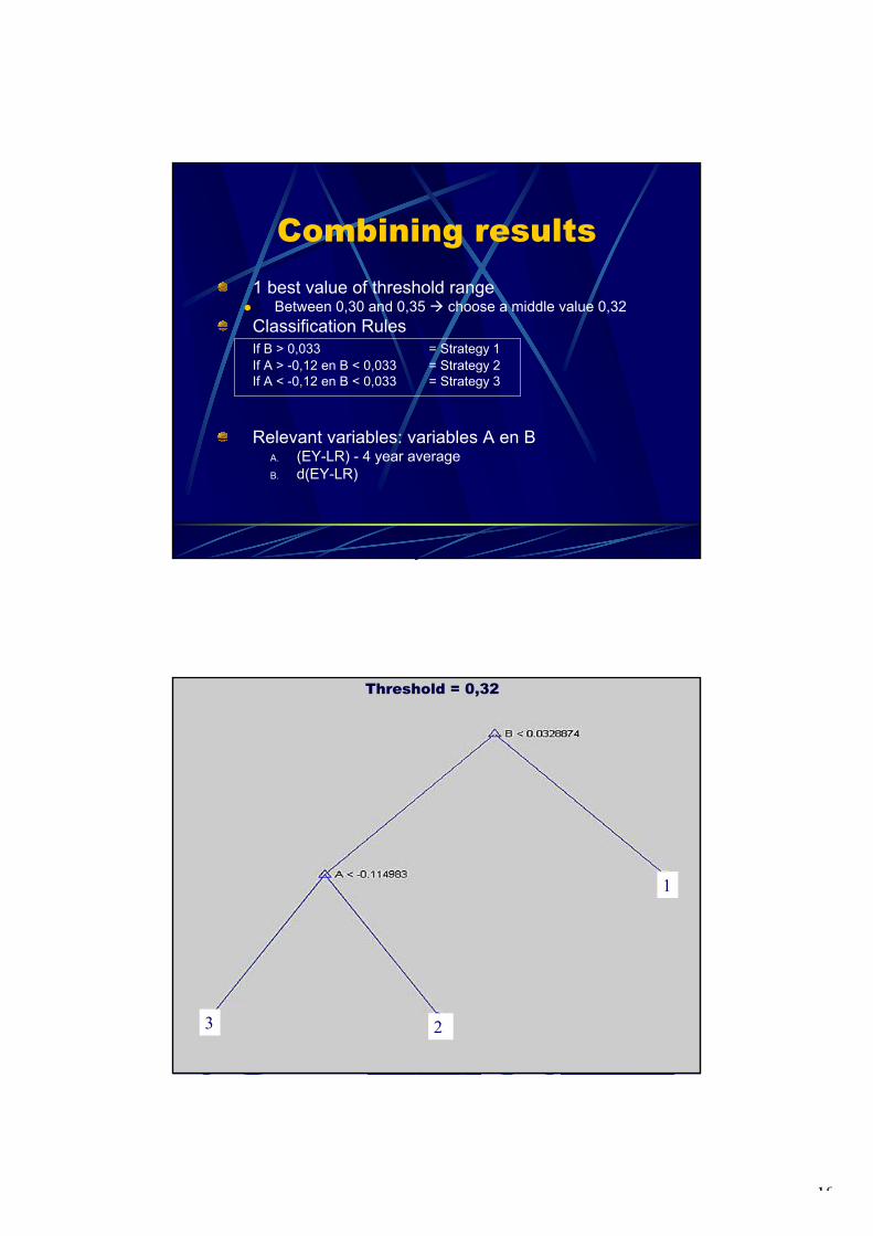
18

Combining results1 best value of threshold range

Between 0,30 and 0,35 choose a middle value 0,32Classification RulesIf B > 0,033 = Strategy 1If A > -0,12 en B < 0,033 = Strategy 2If A < -0,12 en B < 0,033 = Strategy 3

Relevant variables: variables A en BA. (EY-LR) - 4 year averageB. d(EY-LR)

Threshold = 0,32

3 2

1

19

ConclusionThe best threshold value = 0,32; three classification rules from CARTExpect higher return than standard portfolio by using these rules2 most relevant variables, A and BGoals achieved

Gain insight to relevant variablesA high-performed tool, consists of rules, to select investment strategy

Future research What we do: Basic approach ~ simple and understandableAlternatives methods and improvements

More than 3 investment strategies Generalization of the methodOther AI techniquesMore / Less Assumptions about the worldOther indicator variables

20

Discussion

Questions?

ARA model

6 relevant variables Threshold van 20%Each variables is transform to -1, 0 en +1 (negative, neutral, positive signal)Final signal: weighted average of all variables’ signalsOutput: prediction of next month ER

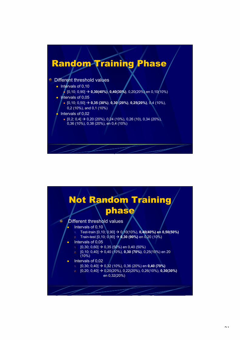
21

Random Training PhaseDifferent threshold values

Intervals of 0,10 [0,10; 0,90] 0,30(40%), 0,40(30%), 0,20(20%) en 0,10(10%)

Intervals of 0,05 [0,10; 0,50] 0,35 (30%), 0,30 (20%), 0,25(20%), 0,4 (10%), 0,2 (10%), and 0,1 (10%)

Intervals of 0,02[0,2; 0,4] 0,20 (20%), 0,24 (10%), 0,26 (10), 0,34 (20%), 0,36 (10%), 0,38 (20%), en 0,4 (10%)

Not Random Training phase

Different threshold valuesIntervals of 0,10 1. Test-train [0,10; 0,90] 0,10(10%), 0,40(40%) en 0,50(50%)2. Train-test [0,10; 0,90] 0,30 (90%) en 0,20 (10%)Intervals of 0,05 1. [0,30; 0,60] 0,35 (50%) en 0,40 (50%)2. [0,10; 0,40] 0,40 (10%), 0,30 (70%), 0,25(10%) en 20

(10%)Intervals of 0,021. [0,30; 0,40] 0,32 (10%), 0,36 (20%) en 0,40 (70%)2. [0,20; 0,40] 0,20(20%), 0,22(20%), 0,26(10%), 0,30(30%)

en 0,32(20%)

1

BASEL II Compliant CreditBASEL II Compliant CreditRisk Management:Risk Management:The OMEGA CaseThe OMEGA Case

Peter van Peter van derder PuttenPutten, KiQ, KiQ(([email protected]@kiq.com))

22ndnd Workshop on Workshop on Smart Adaptive Systems Smart Adaptive Systems in Financein FinanceMay 20 2004May 20 2004

BASEL II and Adaptive Systems

Go together like a horse and carriage?

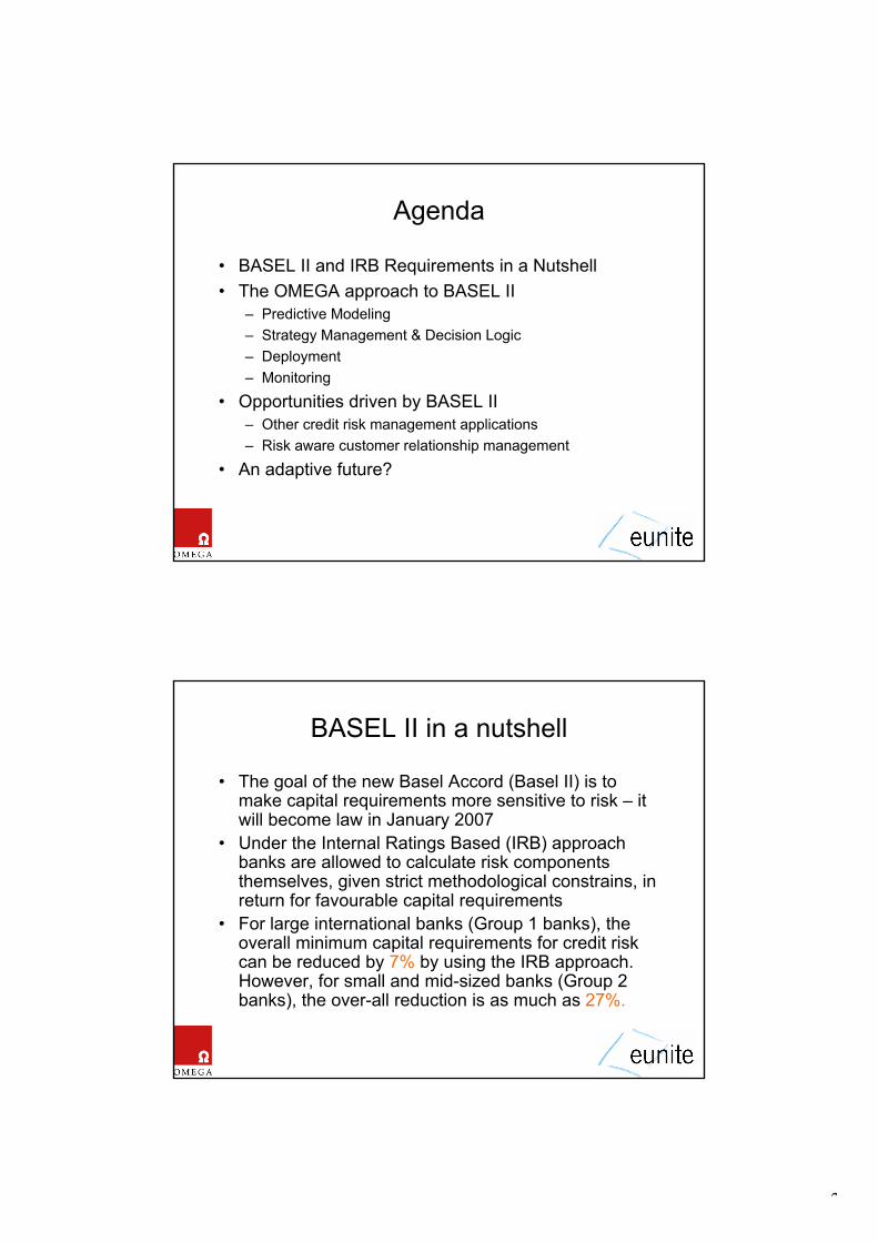
2

Agenda

• BASEL II and IRB Requirements in a Nutshell• The OMEGA approach to BASEL II

– Predictive Modeling– Strategy Management & Decision Logic– Deployment– Monitoring

• Opportunities driven by BASEL II– Other credit risk management applications– Risk aware customer relationship management

• An adaptive future?

BASEL II in a nutshell

• The goal of the new Basel Accord (Basel II) is to make capital requirements more sensitive to risk – it will become law in January 2007

• Under the Internal Ratings Based (IRB) approach banks are allowed to calculate risk components themselves, given strict methodological constrains, in return for favourable capital requirements

• For large international banks (Group 1 banks), the overall minimum capital requirements for credit risk can be reduced by 7% by using the IRB approach. However, for small and mid-sized banks (Group 2 banks), the over-all reduction is as much as 27%.

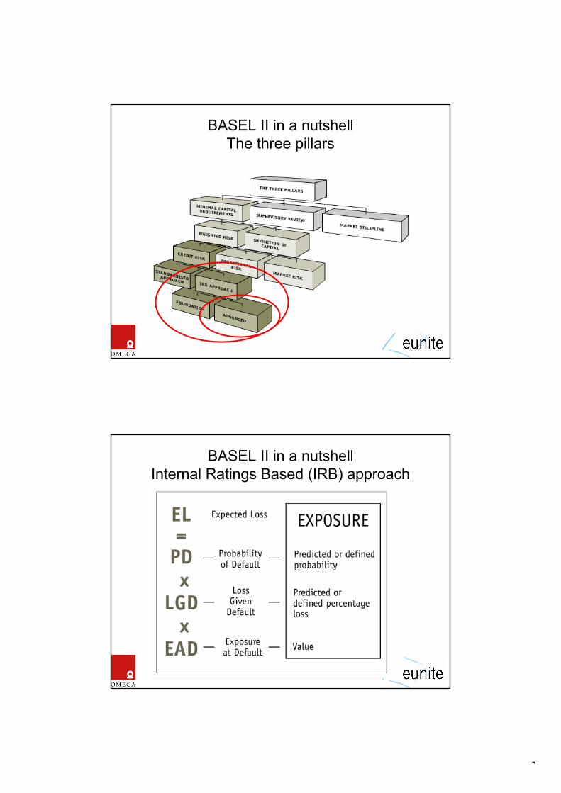
3

BASEL II in a nutshellThe three pillars

BASEL II in a nutshellInternal Ratings Based (IRB) approach

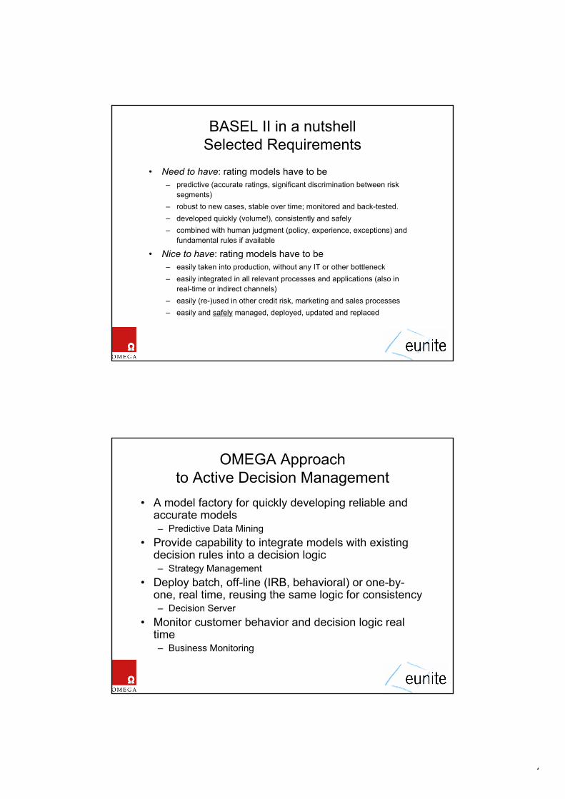
4

• Need to have: rating models have to be– predictive (accurate ratings, significant discrimination between risk

segments)– robust to new cases, stable over time; monitored and back-tested. – developed quickly (volume!), consistently and safely– combined with human judgment (policy, experience, exceptions) and

fundamental rules if available

• Nice to have: rating models have to be– easily taken into production, without any IT or other bottleneck– easily integrated in all relevant processes and applications (also in

real-time or indirect channels)– easily (re-)used in other credit risk, marketing and sales processes– easily and safely managed, deployed, updated and replaced

BASEL II in a nutshellSelected Requirements

OMEGA Approachto Active Decision Management

• A model factory for quickly developing reliable and accurate models– Predictive Data Mining

• Provide capability to integrate models with existing decision rules into a decision logic– Strategy Management

• Deploy batch, off-line (IRB, behavioral) or one-by-one, real time, reusing the same logic for consistency– Decision Server

• Monitor customer behavior and decision logic real time– Business Monitoring

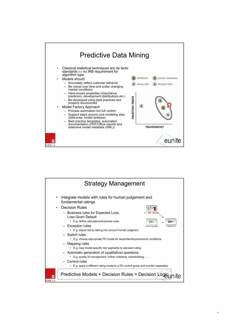
5

Predictive Data Mining

• Classical statistical techniques are de facto standards no IRB requirement for algorithm type

• Models should– Accurately reflect customer behavior– Be robust over time and under changing

market conditions– Have known properties (importance

predictors, development distributions etc.)– Be developed using best practices and

properly documented• Model Factory Approach

– Process automation but full control– Support steps around core modeling step

(data prep, model analysis)– Best practice templates, automated

documentation (PDF/Office reports andextensive model metadata (XML))

Strategy Management

• Integrate models with rules for human judgement and fundamental ratings

• Decision Rules– Business rules for Expected Loss,

Loss Given Default• E.g. define calculations/business rules

– Exception rules• E.g. adjust risk by taking into account human judgment

– Switch rules• E.g. choose appropriate PD model for sector/territory/economic conditions

– Mapping rules• E.g. map model-specific risk segments to standard rating

– Automatic generation of (qualitative) questions• E.g. quality of management, further collateral, shareholding, …

– Control rules• E.g. apply a different rating model to a 5% control group and monitor separately

Predictive Models + Decision Rules = Decision Logic

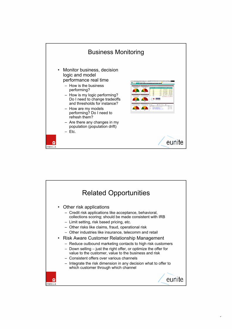
6

Business Monitoring

• Monitor business, decision logic and model performance real time– How is the business

performing?– How is my logic performing?

Do I need to change tradeoffs and thresholds for instance?

– How are my models performing? Do I need to refresh them?

– Are there any changes in my population (population drift)

– Etc.

Related Opportunities

• Other risk applications– Credit risk applications like acceptance, behavioral,

collections scoring; should be made consistent with IRB– Limit setting, risk based pricing, etc.– Other risks like claims, fraud, operational risk– Other industries like insurance, telecomm and retail

• Risk Aware Customer Relationship Management– Reduce outbound marketing contacts to high risk customers– Down selling – just the right offer, or optimize the offer for

value to the customer, value to the business and risk– Consistent offers over various channels– Integrate the risk dimension in any decision what to offer to

which customer through which channel

7

Speculation on an adaptive future

Thank You!

• Summary– We presented selected requirements for (adaptive)

modelling for credit risk modeling in a BASEL II context– Support for the whole managed process of model

development, deployment and monitoring is crucial– OMEGA is an example of a state of an art industry solution– The match between adaptivity and BASEL II is not

straightforward, but there are certainly possibilities

• Questions or requests for white papers: [email protected]

• More info on www.kiq.com

1

Subjective Information and theQuantification of Operational Risks

Dr. Lourenco MirandaABN AMRO

Operational Risk Policy & Support

II Workshop - Smart Adaptive Systems in FinanceRotterdam School of Economics - Erasmus University, RotterdamMay 19, 2004

Definition Operational RiskOperational risk is the risk of loss resulting

from inadequate or failed

• internal processes,• human behaviour,• systems,

or from

• external events

2

Stage 1

BasicIndicatorApproach

Stage 2

StandardisedApproach

Stage 3

AdvancedMeasurementApproaches

- One size fits all- No incentives for

better ORM

- Risk based- Incentive to

manage risks

Simplicity

Granularity

Risk sensitivity

Simple

Low

Less reflective of actual risk

Sophisticated

High

More reflective of actual risk

Sound Practises Paper

Pillar I for Operational Risk

The AMA approach consists of:

Goal: development of a risk based economic capital approach that qualifies for the AMA for regulatory capital

combined with

loss expectations + support

historic loss data + adjustments

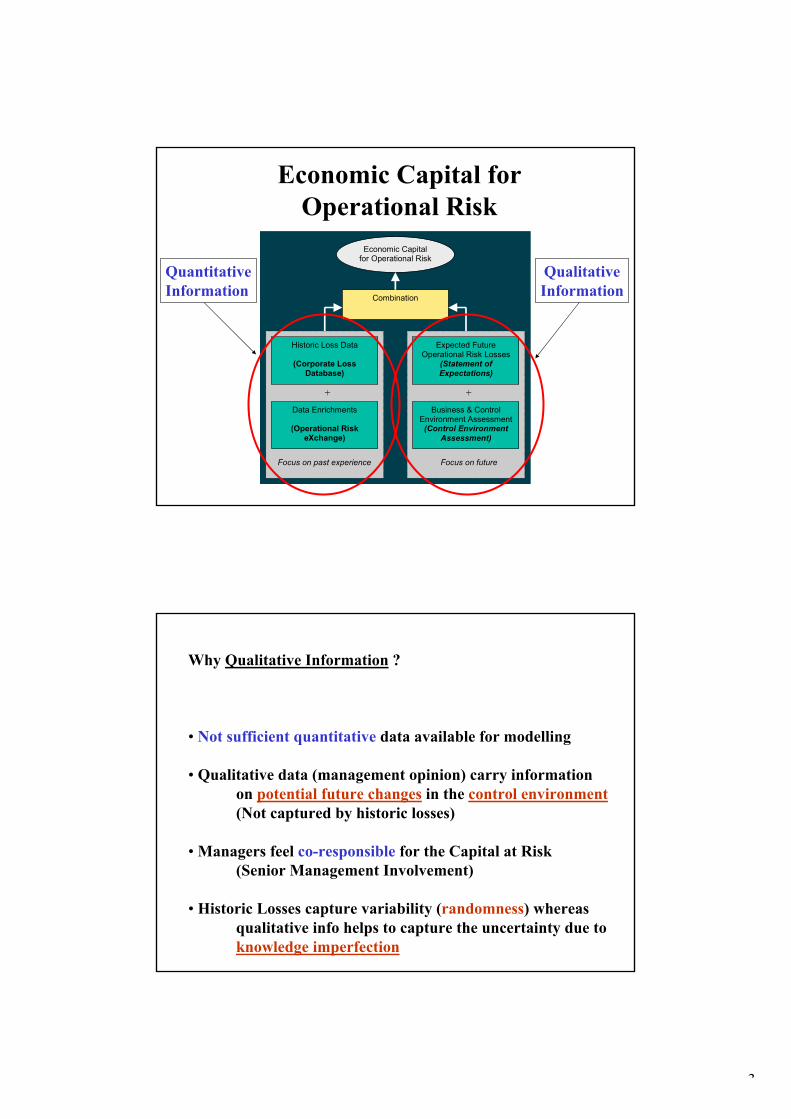
3

Historic Loss Data

(Corporate LossDatabase)

Data Enrichments

(Operational RiskeXchange)

Expected FutureOperational Risk Losses

(Statement ofExpectations)

Business & ControlEnvironment Assessment(Control Environment

Assessment)

Combination

Economic Capitalfor Operational Risk

Focus on past experience Focus on future

+ +

Economic Capital forOperational Risk

QuantitativeInformation

QualitativeInformation

Why Qualitative Information ?

• Not sufficient quantitative data available for modelling

• Qualitative data (management opinion) carry informationon potential future changes in the control environment(Not captured by historic losses)

• Managers feel co-responsible for the Capital at Risk(Senior Management Involvement)

• Historic Losses capture variability (randomness) whereasqualitative info helps to capture the uncertainty due toknowledge imperfection

4

Treating Qualitative Information:

• Credibility Theory

• Bayesian Approach

• Smart Adaptive Systems (SAS)Ex: Fuzzy Logic

Fuzzy Logic and Operational Risk

• Processes qualitative knowledge (rich in info)

• Tries to quantify qualitative information - generate innumerical terms the Operational Risk faced by an institution

• Fuzzy multi-attribute (risk factors) evaluation problem

• Fuzzy Linguistic Labels assigned to Risk Factors (Causes)(Causal Modelling)

• A causal model is used to develop a distribution of losses basedon management expectations for the levels of therisk factors

5


• First step: Specification of Risk Factors and related indicators

• An indicator can be a specific causal variable (frequently measured)

• Ex: Number of Documents with ErrorsAudit score for the businessExperience of Employees (Years)Employee Turnover


• 2nd: Calibration of Fuzzy Representation of the Indicators

• Use linguistic variables to represent the indicators

• Do the same with the loss amount correspondent to this risk

• High / Medium / Low (H/M/L) scale is used

• Basis for capturing expert opinion on the impact of the indicatorson the loss amount

• Calibrating depends upon the understanding and interpretation ofthe managers towards the H/M/L scale

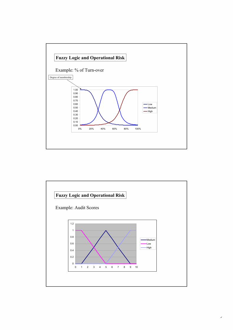
6


0.000.100.200.300.400.500.600.700.800.901.00

0% 20% 40% 60% 80% 100%

LowMediumHigh

Example: % of Turn-overDegree of membership

Example: Audit Scores


0

0.2

0.4

0.6

0.8

1

1.2

0 1 2 3 4 5 6 7 8 9 10

MediumLowHigh

7

0

0.2

0.4

0.6

0.8

1

1.2

0 200 400 600 800 1000 1200

MediumLowHigh

Example: Total Loss (in 1,000 EUR)



• 3rd - specify impact of indicators on Loss Amount• Loss Amount => “Function” of the Indicators

• Reasoning: Fuzzy Rules => If… then…

If <% of Turnover> is Highand

<Audit Score > is Lowthen

<Loss Amount> is Moderate

Rules span all possible scenarios for combination of the levels ofthe indicators - a complete map is made to the output space(loss amounts)

8


4th - Apply a Defuzzification Rule to Calculate the Estimated Losses

• Estimated losses can be calculated for each combination of rule• A fuzzy calculator (defuzzifier) is applied to estimate the losses

• The distribution of actual losses is modified by thedistribution of estimated losses (which come from thecombination of the levels of the indicators)

Ex: % of turnover: 63%Audit Score: 7Estimated loss: 650 (1,000 EUR)


• Fuzzy logic approach provides more information to the riskmanagement process

• Risks are quantified based on a combination of historical datahistorical data andexpert inputexpert input

• Due to the (subjective) nature of Operational Risk, there is a wideopen field of possible applications of Smart Adaptive Systems

• Operational Risk has become a rich subject for soft computingand SAS - yet, there is so much to be done…

Final remarks

DECISIONMETRICS: DYNAMIC

STRUCTURAL ESTIMATION OF

SHIPPING INVESTMENT DECISIONS

George Dikos

Massachusetts Institute of Technology

Monday, March 29, 2004

1

PROJECT DEFINITION AND

ULTIMATE GOAL

Project Definition:Develop Structural Equilibrium

Models for Real and Auxiliary Markets.

Ultimate Goal: Structural Estimation: Use Eco-

nomic Theory to determine the Functional Form. (Strong

Policy Implications)

2

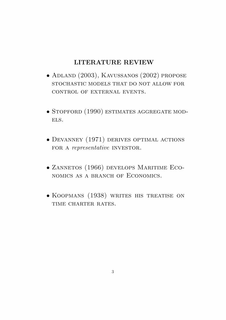
LITERATURE REVIEW

• Adland (2003), Kavussanos (2002) propose

stochastic models that do not allow for

control of external events.

• Stopford (1990) estimates aggregate mod-

els.

• Devanney (1971) derives optimal actions

for a representative investor.

• Zannetos (1966) develops Maritime Eco-

nomics as a branch of Economics.

• Koopmans (1938) writes his treatise on

time charter rates.

3

CONTRIBUTIONS

1. Structural Models based on the “Bottom-

Up” approach.

• Data are aggregate and not individ-

ual.

• How can individual optimal actions be

aggregated to explain aggregate co-

movements?

2. ESTIMATION and SPECIFICATION

• Employ Economic Theory to test eco-

nomic assertions and reduce dimension-

ality.

• Employ modern Econometrics.

4

Aggregate Shipping Investment Decisions

Three Party Model

• Actions of Entry.

• Lay-Up or Charter decisions of the ex-

isting fleet.

• Actions of Exit.

Assumption: The prevailing time charter

rate is EXOGENOUS for investment deci-

sions of entry and exit.

Why is the time charter rate exogenous?

• Dornbusch-Fischer, “Macroeconomics” (1987)

• There is a construction lag between in-

vestment orders and employment of the

new vessel.

• The deadweight ordered is relatively small

compared to the existing fleet.

5

ESTIMATION METHODS: Divide and

Conquer

Advanced estimation and specification tech-

niques are employed.

1. Entry and exit are count data.

• Poisson, Negative Binomial Fixed and

Random Effects Models.

• Tobit and Median Regression for cen-

sored deadweight orders.

2. Prices are time series data.

• Auto Regressive Moving Average and

Generalized Auto Regressive Condi-

tional Heteroscedastic models are de-

rived and estimated in a structural

framework.

• System Dynamics.

3. Real Option Pricing of second hand ves-

sels.

6

Figure 1: System Dynamics Modelling of Freight Rates

7

MODULE 1: ENTRY

• PERFECT COMPETITION

• Newbuilding decisions are exogenous

• Time charter rates

• Existence of organized markets

• Demand for transportation capacity is

inelastic in the short term

• Payoffs

8

WHY THE REAL OPTION MARKUP?

Key Identification Device: Market Com-

pleteness

Under the assumption of complete mar-

kets the value of this project is uniquely

spanned in financial markets.

We do not need to solve each agents’ Dy-

namic Programming Problem.

Key Assumption-Reducing Dimensionality :

Freight Markets are complete (Baltic Ex-

change) and the Real Option Value is a SUF-

FICIENT STATISTIC for characterizing in-

vestment decisions.

Still unexplained: Differences among op-

erating the vessels, small premia achieved

due to networks and the number of poten-

tial investors. Econometric error neces-

sary to make the model NON-DEGENERATE.

9

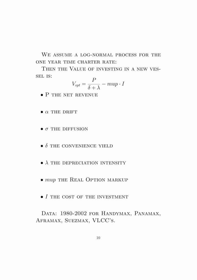
We assume a log-normal process for the

one year time charter rate:

Then the Value of investing in a new ves-

sel is:

Vopt =P

δ + λ− mup · I

• P the net revenue

• α the drift

• σ the diffusion

• δ the convenience yield

• λ the depreciation intensity

• mup the Real Option markup

• I the cost of the investment

Data: 1980-2002 for Handymax, Panamax,

Aframax, Suezmax, VLCC’s.

10

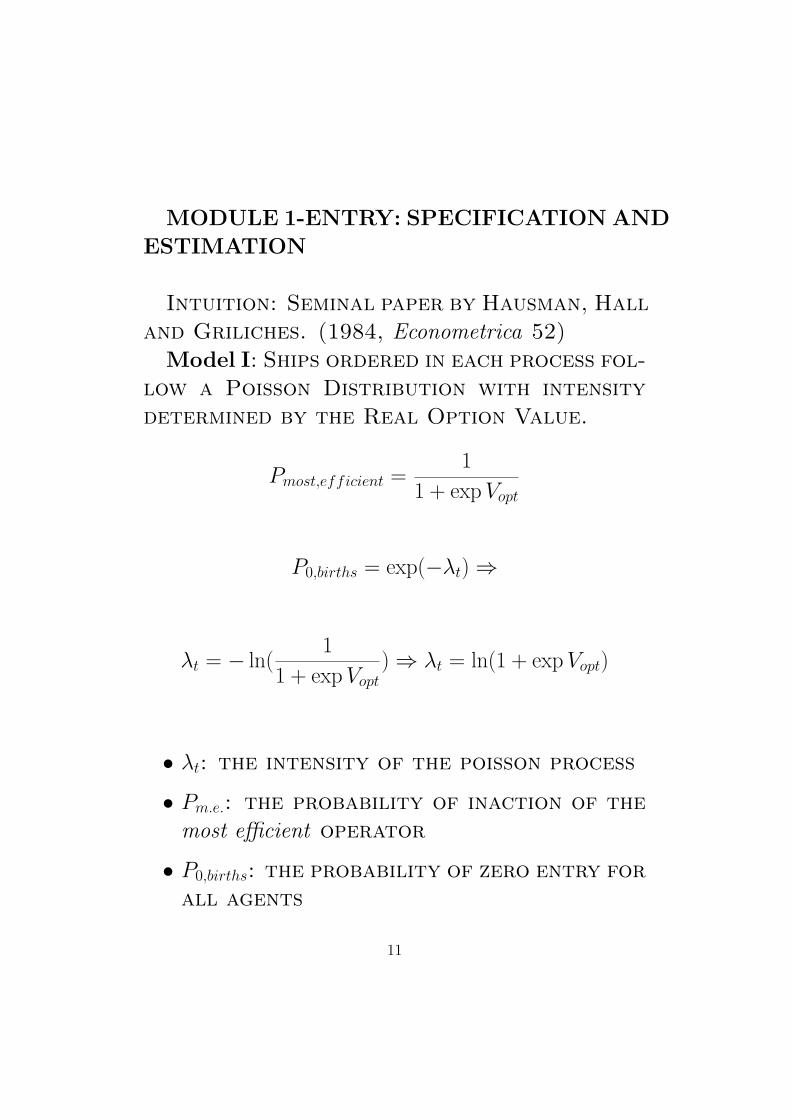
MODULE 1-ENTRY: SPECIFICATION AND

ESTIMATION

Intuition: Seminal paper by Hausman, Hall

and Griliches. (1984, Econometrica 52)

Model I: Ships ordered in each process fol-

low a Poisson Distribution with intensity

determined by the Real Option Value.

Pmost,efficient =1

1 + exp Vopt

P0,births = exp(−λt) ⇒

λt = − ln(1

1 + exp Vopt) ⇒ λt = ln(1 + exp Vopt)

• λt: the intensity of the poisson process

• Pm.e.: the probability of inaction of the

most efficient operator

• P0,births: the probability of zero entry for

all agents

11

Figure 2: Tonnage Ordered across Categories 1980-2002(q)F

igu

re 1

: T

on

na

ge

Ord

ere

d a

cro

ss

Ca

teg

ori

es

19

80

-20

02

(q)

012345678

80.1

80.4

81.3

82.2

83.1

83.4

84.3

85.2

86.1

86.4

87.3

88.2

89.1

89.4

90.3

91.2

92.1

92.4

93.3

94.2

95.1

95.4

96.3

97.2

98.1

98.4

99.3

2000,2

2001,1

2001,4

2002,3

19

80

- 2

00

2 (

q)

Tonnage in MT

20

0 K

DW

T

90

KD

WT

10

KD

WT

12

Model I Results

Model NLLS PQMLE NB OLS

lnPm.e. .3239 (.012) .2901 (.028) .3461 (.040) 2.691 (.352)const 1.553 (.027) 1.622 (.067) 1.520 (.071) 4.468 (.380)

Log likelihood -2413 -1623 -1358 n.a.PseudoR2 0.1267 n.a. 0.0258 0.1451

• NLLS: Non Linear Least Squares

• PQMLE: Partial Quasi Maximum Likeli-

hood Estimation

• NB: Negative Binomial

• OLS: Ordinary Least Squares

Hausman test between NLLS and Poisson:

1.65

Pearson statistic normalized for 454 d.o.f.

is 74.9, which is evidence for overdispersion.

The “Goodness of Fit” is χ2 = 3447.

We clearly reject this model, but pro-

ceed with fixed and random effects.

13

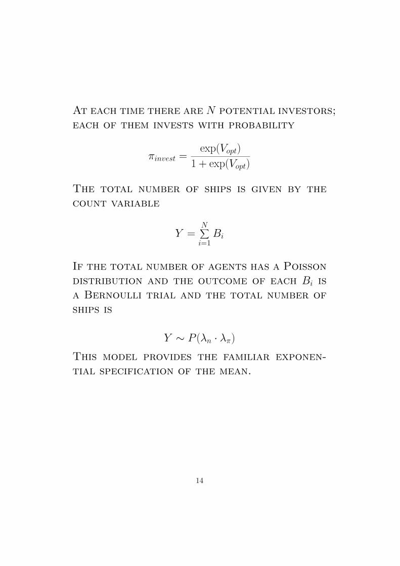
At each time there are N potential investors;

each of them invests with probability

πinvest =exp(Vopt)

1 + exp(Vopt)

The total number of ships is given by the

count variable

Y =N∑

i=1Bi

If the total number of agents has a Poisson

distribution and the outcome of each Bi is

a Bernoulli trial and the total number of

ships is

Y ∼ P (λn · λπ)

This model provides the familiar exponen-

tial specification of the mean.

14

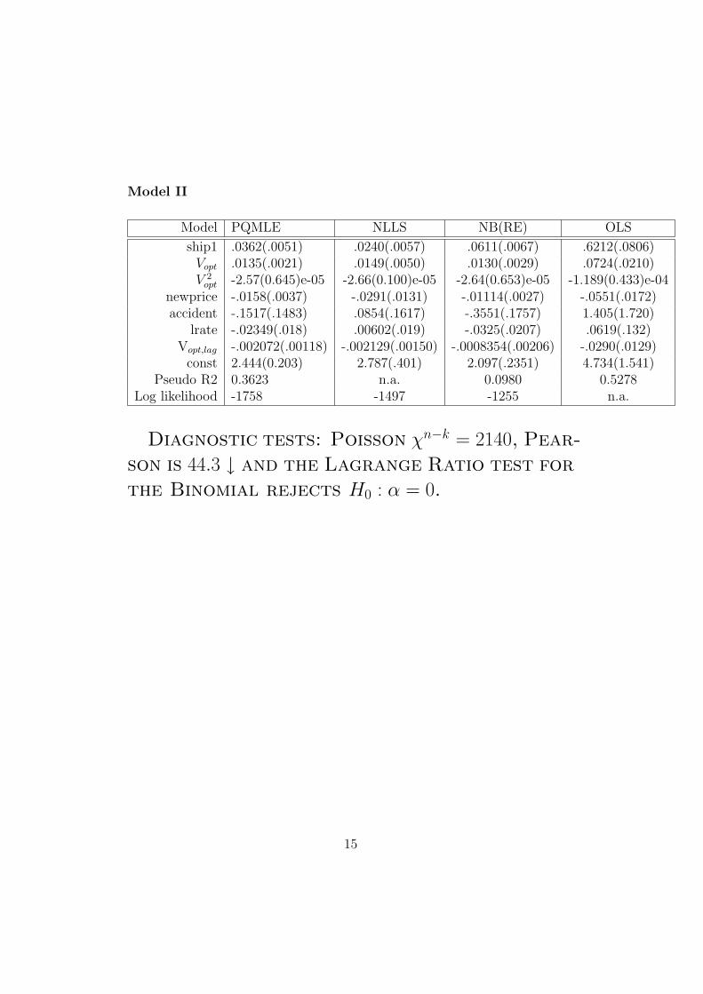
Model II

Model PQMLE NLLS NB(RE) OLS

ship1 .0362(.0051) .0240(.0057) .0611(.0067) .6212(.0806)Vopt .0135(.0021) .0149(.0050) .0130(.0029) .0724(.0210)V 2

opt -2.57(0.645)e-05 -2.66(0.100)e-05 -2.64(0.653)e-05 -1.189(0.433)e-04newprice -.0158(.0037) -.0291(.0131) -.01114(.0027) -.0551(.0172)accident -.1517(.1483) .0854(.1617) -.3551(.1757) 1.405(1.720)

lrate -.02349(.018) .00602(.019) -.0325(.0207) .0619(.132)Vopt,lag -.002072(.00118) -.002129(.00150) -.0008354(.00206) -.0290(.0129)const 2.444(0.203) 2.787(.401) 2.097(.2351) 4.734(1.541)

Pseudo R2 0.3623 n.a. 0.0980 0.5278Log likelihood -1758 -1497 -1255 n.a.

Diagnostic tests: Poisson χn−k = 2140, Pear-

son is 44.3 ↓ and the Lagrange Ratio test for

the Binomial rejects H0 : α = 0.

15

We now relax the Real Option Linear Parametriza-

tion.

The results are very supportive:

• The coefficient of tc an op are of the

same order and have the required signs.

• The op is slightly higher since costs in-

cur even when the ship does not earn

revenue (dry-dock, in port).

• tc and op are on per day basis. If we mul-

tiply the difference by 365 we get the

same order with newprice.

• In the semi-parametrized table the im-

plied markup is close to 4.

If Vopt is correctly specified the estimates

are efficient; if not they are inconsistent.

We do a Hausman test between the Full

Linear Parametrization and the Real Op-

tion specification.

RESULT: χ2(6) = 1.62 NOT REJECT THE

REAL OPTION COMBINATION.

16

MODULE 2-EXIT: SPECIFICATION

Key Questions

• Derive models for aggregate exit data.

• Exit Decisions or Capital Replacement

Decisions?

• Stabilizing or Destabilizing Force?

17

MODULE 2-EXIT: ESTIMATION AND

CONCLUSIONS

1. Estimation

• Count Data Models.

• Auto Regressive Moving Average mod-

els for aggregate scrapped deadweight.

• White Noise Tests (Bartlett), Instru-

mental Variables, Double 2 Stage Least

Absolute Deviations and Quantile Re-

gression estimation methods.

• Hausman Tests.

2. Conclusions

• Scrapping Decisions are mainly Exit

Decisions and NOT Capital Replace-

ment Decisions.

• Scrapping Decisions are a small frac-

tion of the total fleet.

• Equilibrium Models sufficiently explain

scrapping activity.

18

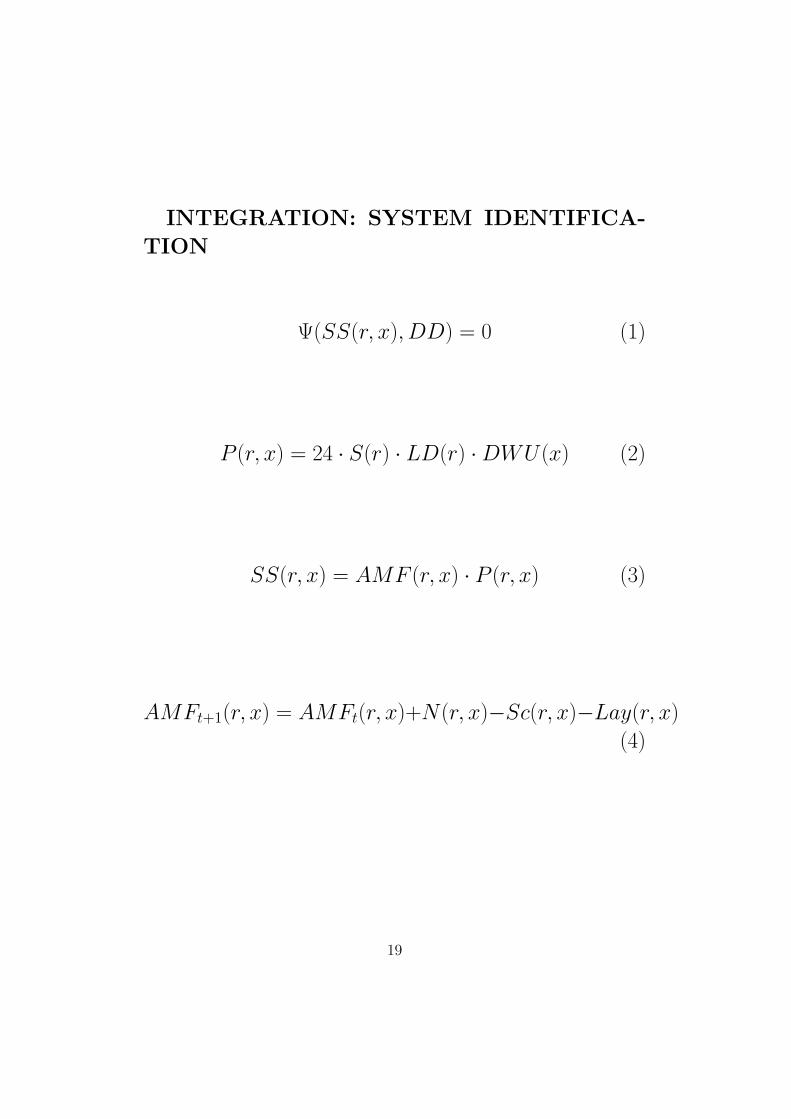
INTEGRATION: SYSTEM IDENTIFICA-

TION

Ψ(SS(r, x), DD) = 0 (1)

P (r, x) = 24 · S(r) · LD(r) · DWU(x) (2)

SS(r, x) = AMF (r, x) · P (r, x) (3)

AMFt+1(r, x) = AMFt(r, x)+N(r, x)−Sc(r, x)−Lay(r, x)

(4)

19

• SS: transportation supply function in ton-

miles

• DD: exogenous transportation demand in

ton-miles

• r: the time charter freight rate at time

• x: all other exogenous variables

• AMF: average merchant fleet

• P: average fleet productivity

• N,Sc,Lay: newbuilding, scrapped and ton-

nage in lay-up

• S: velocity

• LD: loaded days at sea

• DWU: deadweight utilization

20

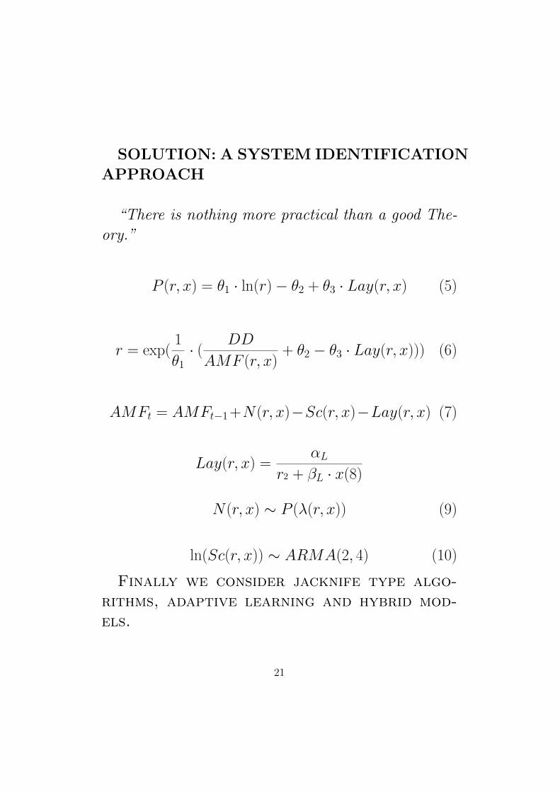
SOLUTION: A SYSTEM IDENTIFICATION

APPROACH

“There is nothing more practical than a good The-

ory.”

P (r, x) = θ1 · ln(r) − θ2 + θ3 · Lay(r, x) (5)

r = exp(1

θ1· ( DD

AMF (r, x)+ θ2 − θ3 · Lay(r, x))) (6)

AMFt = AMFt−1+N(r, x)−Sc(r, x)−Lay(r, x) (7)

Lay(r, x) =αL

r2 + βL · x(8)

N(r, x) ∼ P (λ(r, x)) (9)

ln(Sc(r, x)) ∼ ARMA(2, 4) (10)

Finally we consider jacknife type algo-

rithms, adaptive learning and hybrid mod-

els.

21

MIXED STRATEGY: A HYBRID MODEL

rt =d∑

j=1arLj·rt−j+X ′

t·β+q∑

k=0maLk·εt−k, εt ∼ N(0, σ2

t )

(11)

ln σ2t =

p∑

j=1earchLj·ln σ2

t−j+Z ′t·hetfactors+

q∑

k=0egarchLk·zt−k

(12)

zt ∼ N(0, σ2) (13)

22

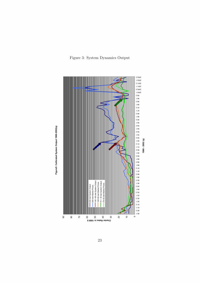
Figure 3: System Dynamics OutputF

igu

re5

: C

ali

bra

ted

Sy

ste

m O

utp

ut

19

80

-20

02

(q)

0

10

20

30

40

50

60

70

80

90

80.1

80.3

81.1

81.3

82.1

82.3

83.1

83.3

84.1

84.3

85.1

85.3

86.1

86.3

87.1

87.3

88.1

88.3

89.1

89.3

90.1

90.3

91.1

91.3

92.1

92.3

93.1

93.3

94.1

94.3

95.1

95.3

96.1

96.3

97.1

97.3

98.1

98.3

99.1

99.3

2000,1

2000,3

2001,1

2001,3

2002,1

2002,3

19

80

- 2

00

2 (

q)

Charter Rates in 1000 $

20

0 d

wt

Syste

m O

utp

ut

20

0 d

wt

Ma

rke

t P

rice

s

14

0 +

90

dw

t S

yste

m O

utp

ut

14

0+

90

dw

t M

ark

et

Price

s

70

+ 3

0 d

wt

Syste

m O

utp

ut

70

+3

0 d

wt

Ma

rke

t P

rice

s

��

��

��

23

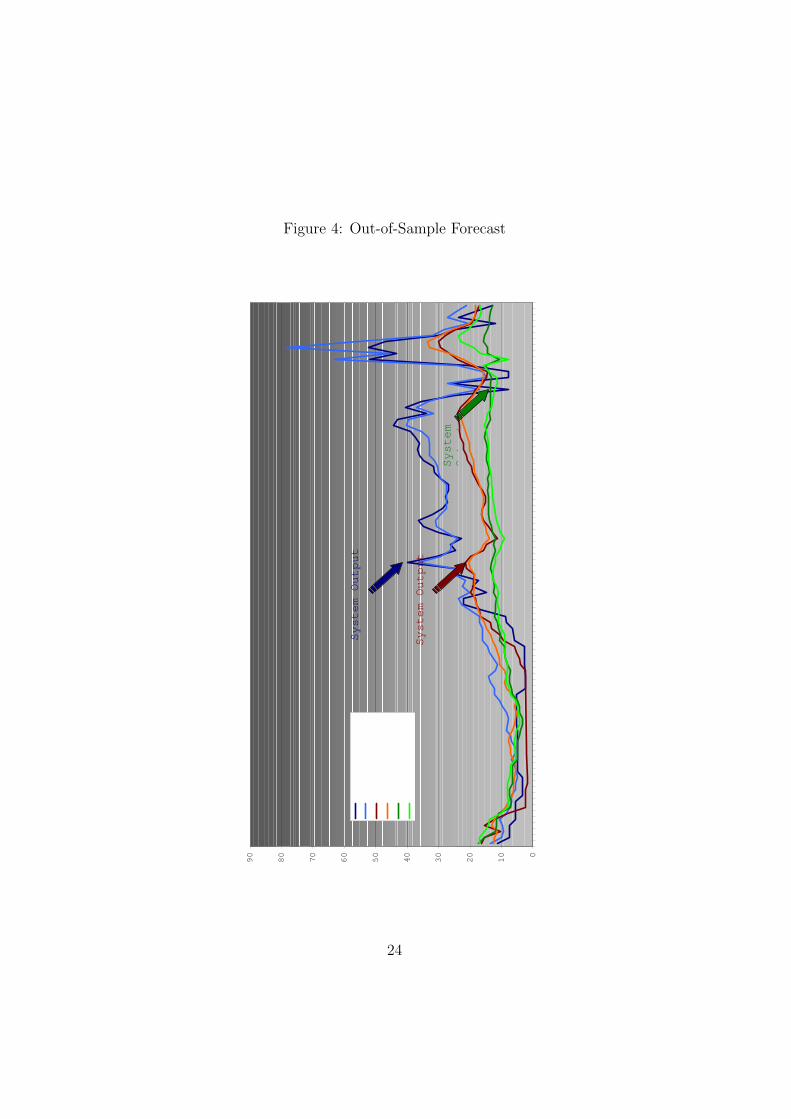
Figure 4: Out-of-Sample Forecast��

0

10

20

30

40

50

60

70

80

90

��

��

��

��

��

��

��

��

��

��

��

��

��

��

��

��

��

��

��

��

��

��

��

��

��

��

��

��

��

��

��

��

��

��

��

��

��

��

��

��

��

��

��

��

��

��

��

��

��

��

��

��

��

��

System Output

System Output

System

Output

24

CONCLUSIONS

WE HAVE SUCCESSFULLY INTEGRATED

THE THREE DIFFERENT SUB-MODULES.

• The Real Option Value is a sufficient

statistic for entry.

• Scrapping Decisions are Not Capital Re-

placement Decisions but Exit Decisions.

• Demand is a sufficient statistic for equi-

librium prices.

• Newbuilding prices are demand inelastic.

• Re-address early hypotheses in Maritime

Economics.

• Provide Quantitative Evidence to sev-

eral assertions (Zannetos, Devanney) in

a “Bottom-Up” structural framework.

25

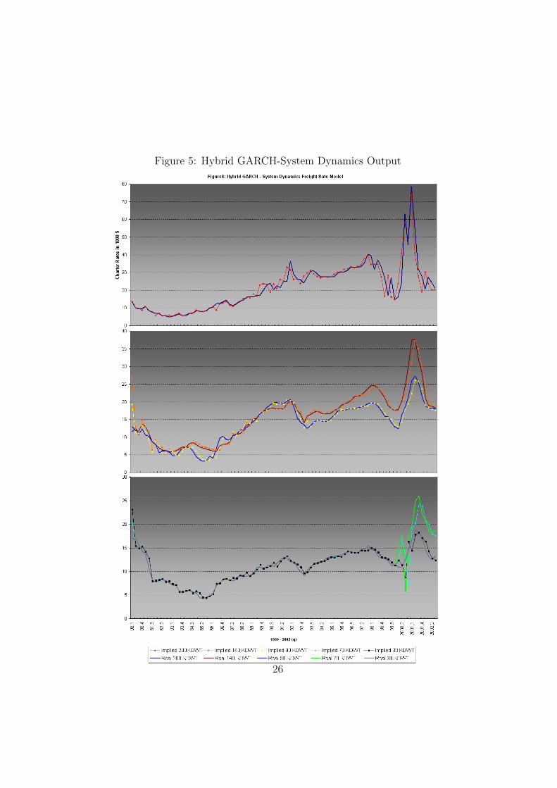
Figure 5: Hybrid GARCH-System Dynamics Output

26

1

1

Extending the OLAP framework Extending the OLAP framework for automated diagnosisfor automated diagnosisof business performanceof business performance

Erasmus University Rotterdam, May 19, 2004Emiel Caron ([email protected])

special thanks to: Tony Brabazon, University College Dublin

Hennie Daniels, Erasmus University Rotterdam

2

ResearchResearch objectiveobjective

On-Line Analytical Processing (OLAP) provides a framework for analysis of multidimensional business data

Problem: OLAP systems have no support for automated business diagnosis/comparison tasks

Objective: Extend OLAP framework with explanation formalism for automated business diagnosis & propose algorithm

Question: How can the OLAP framework be extended with an explanation formalism?

2

3

OverviewOverview ofof PresentationPresentation

On-Line Analytical Processing (OLAP)

General model for automated diagnosis of business performance

Extending OLAP with explanation capabilities & some example calculations

4

Part I:Part I:

OLAPOLAP

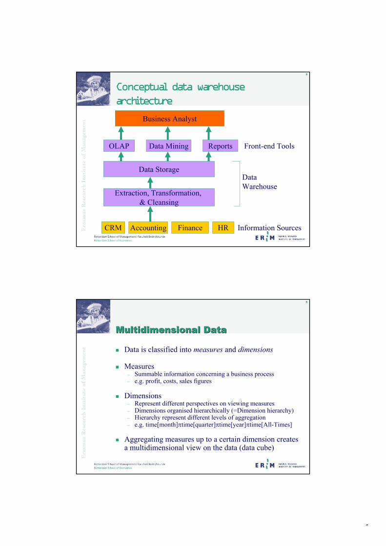
3

5

Conceptual data warehouse architecture

Business Analyst

OLAP Data Mining Reports

Data Storage

Extraction, Transformation, & Cleansing

CRM Accounting Finance HR

DataWarehouse

Front-end Tools

Information Sources

6

MultidimensionalMultidimensional DataData

Data is classified into measures and dimensions

Measures– Summable information concerning a business process– e.g. profit, costs, sales figures

Dimensions– Represent different perspectives on viewing measures– Dimensions organised hierarchically (=Dimension hierarchy)– Hierarchy represent different levels of aggregation– e.g. time[month] time[quarter] time[year] time[All-Times]

Aggregating measures up to a certain dimension creates a multidimensional view on the data (data cube)

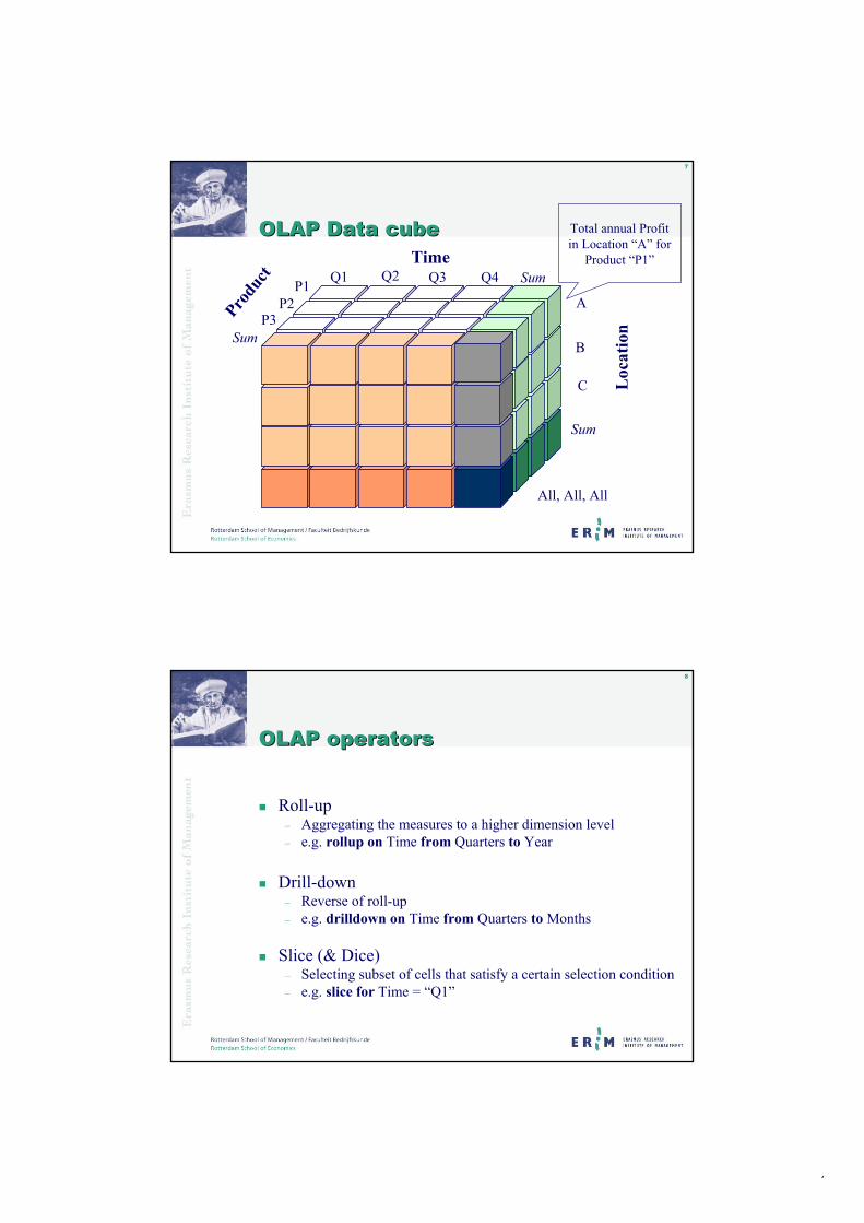
4

7

OLAP Data OLAP Data cubecubeTime

Produ

ct

Loc

atio

nSum

SumP1

P3P2

Q1 Q2 Q3 Q4

A

B

C

Sum

All, All, All

Total annual Profitin Location “A” for

Product “P1”

8

OLAP operatorsOLAP operators

Roll-up– Aggregating the measures to a higher dimension level– e.g. rollup on Time from Quarters to Year

Drill-down– Reverse of roll-up– e.g. drilldown on Time from Quarters to Months

Slice (& Dice)– Selecting subset of cells that satisfy a certain selection condition– e.g. slice for Time = “Q1”

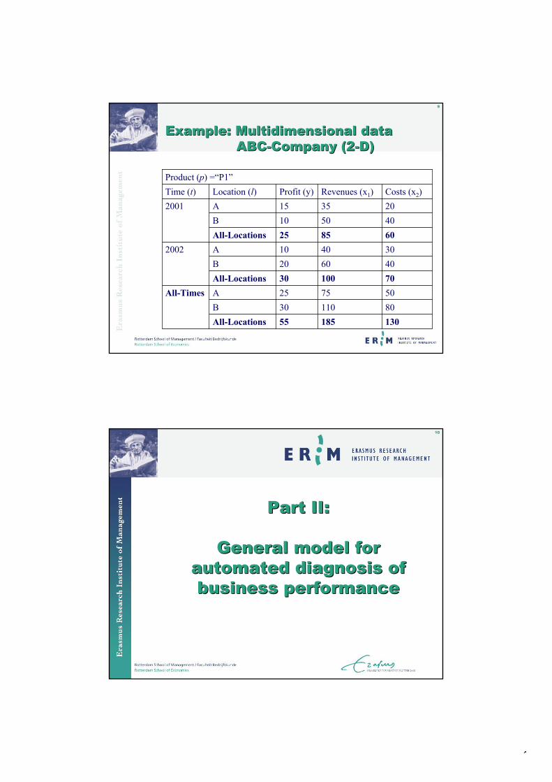
5

9

ExampleExample:: Multidimensional Multidimensional datadataABCABC--Company Company (2(2--D)D)

13018555All-Locations8011030B507525AAll-Times7010030All-Locations406020B304010A2002608525All-Locations405010B203515A2001Costs (x2)Revenues (x1)Profit (y)Location (l)Time (t)

Product (p) =“P1”

10

Part II:Part II:

General model for General model for automated diagnosis of automated diagnosis of business performancebusiness performance

6

11

Diagnostic problem solvingDiagnostic problem solving

Diagnosis: “finding the best explanation of observed abnormal behaviour (or observed symptoms) of a system”

Symptoms: profit , sales(2003)

Knowledge structures for automated business diagnosis:– Norm model– Business model

businessmodel

actualbehaviour

expectedbehaviour

normmodel

Symptom

observations prediction

12

Norm modelNorm model

“Reference objects” to diagnose business performance:

Actual against historical values

Actual against industry averages

Actual against budgeted values

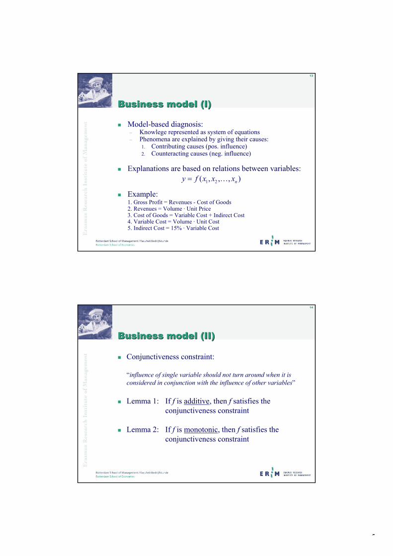
7

13

Business model (I)Business model (I)

Model-based diagnosis:– Knowlege represented as system of equations– Phenomena are explained by giving their causes:

1. Contributing causes (pos. influence)2. Counteracting causes (neg. influence)

Explanations are based on relations between variables:

Example:1. Gross Profit = Revenues - Cost of Goods2. Revenues = Volume · Unit Price3. Cost of Goods = Variable Cost + Indirect Cost4. Variable Cost = Volume · Unit Cost5. Indirect Cost = 15% · Variable Cost

1 2( , , , )ny f x x x

14

Business model (II)Business model (II)

Conjunctiveness constraint:

“influence of single variable should not turn around when it is considered in conjunction with the influence of other variables”

Lemma 1: If f is additive, then f satisfies the conjunctiveness constraint

Lemma 2: If f is monotonic, then f satisfies the conjunctiveness constraint

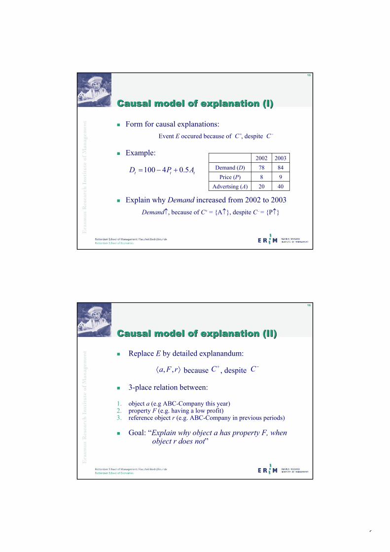
8

15

CausalCausal model of model of explanationexplanation (I)(I)

Form for causal explanations:Event E occured because of , despite

Example:

Explain why Demand increased from 2002 to 2003Demand , because of C+ = {A }, despite C– = {P }

C C

4020Advertsing (A)98Price (P)

8478Demand (D)20032002

100 4 0.5t t tD P A

16

CausalCausal model of model of explanationexplanation (II)(II)

Replace E by detailed explanandum:

because , despite

3-place relation between:

1. object a (e.g ABC-Company this year)2. property F (e.g. having a low profit)3. reference object r (e.g. ABC-Company in previous periods)

Goal: “Explain why object a has property F, when object r does not”

C C, ,a F r

9

17

Example Example ABCABC--CompanyCompany

Interested in ABC-Company’s profit:

Profit = Revenues – Costs ( )

Data for ABC-Company:

Explain why ABC-Company’s profit is low in 2002:<ABC(2002), Profit , ABC(2001)> because C+ = {Revenues , Costs } despite C– = {}

1110x2

1920x1

810y20022001

1 2y x x

18

Part III:Part III:

Extending OLAP with Extending OLAP with explanation capabilitiesexplanation capabilities

10

19

Explanation directionsExplanation directions in OLAPin OLAP

1. Measures (business model equations):

2. Dimensions (drilldown equations):

1( ) ( ( ), , ( ))ny f x xd d d

[quarter] [year]t t

profit( , ) revenues( , ) costs( , )t l t l t l

(2003,A) (2003.q1,A) (2003.q2,A)y y y

1 2(2003,A) (2003,A) (2003,A)y x x

General:Example:

Instances:

[ ] [ ]k kd p d q

(2003.q3,A) (2003.q4,A)y y

General:Example:

Instances:

1( , , )md dd

20

Additive cube functionAdditive cube function

1. y is an additive cube function in dimension dk with dimension hierarchy with levels p and q, and level instances a en b if:

2. y is an additive cube function in dimension dk if def. 1 holds in all dimension levels of the dimension hierarchy

3. y is an additive cube function if def. 2 holds for all dimensions inthe dimension vector d

1( , [ ]. , ) ( , [ ]. , )

n

k k ii

y d q b y d p a

[ ]. [ ].k kd p d q ba

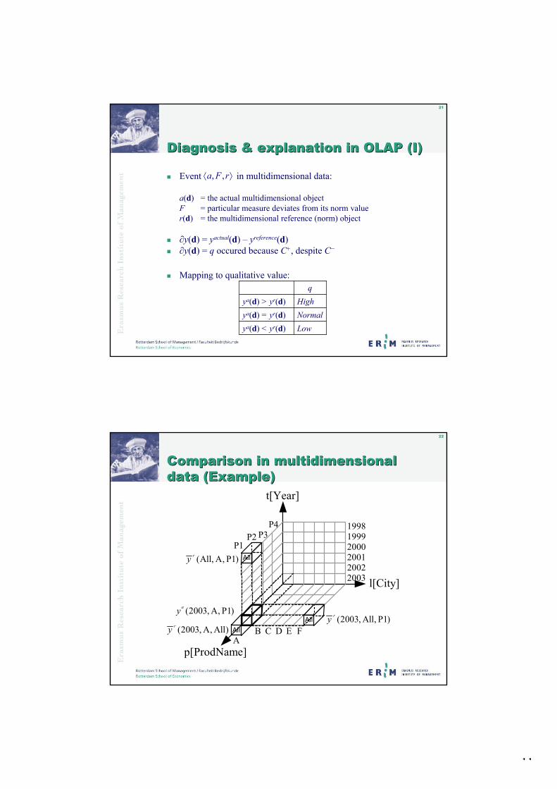
11

21

Diagnosis & Diagnosis & explanation explanation in OLAP (I)in OLAP (I)

Event in multidimensional data:

a(d) = the actual multidimensional objectF = particular measure deviates from its norm valuer(d) = the multidimensional reference (norm) object

y(d) = yactual(d) – yreference(d)y(d) = q occured because C+, despite C–

Mapping to qualitative value:

, ,a F r

Lowya(d) < yr(d)Normalya(d) = yr(d)Highya(d) > yr(d)

q

22

ComparisonComparison in in multidimensionalmultidimensionaldata (data (ExampleExample))

t[Year]

l[City]

p[ProdName]

200320022001200019991998P4

P3P2P1

AB C D E F

(2003, A, P1)ay(2003, All, P1)ry

(All, A, P1)ry

(2003, A, All)ry All

All

All

12

23

Diagnosis & Diagnosis & explanationexplanation in OLAP in OLAP (II)(II)

Influence measure:

“Indicates what the difference between the actual and norm value of y(d) would have been if only xi(d) would have deviated from its norm value”

Influence measure for additive functions:

1 1 1inf( ( ), ( )) ( ( ), , ( ), ( ), ( ), , ( )) ( )r r a r r ri i i i nx y f x x x x x yd d d d d d d d

inf( ( ), ( )) ( ) ( )a ri i ix y x xd d d d

24

Diagnosis & Diagnosis & explanationexplanation in OLAP in OLAP (III)(III)

Contributing causes. Set of contributing causes C+ consists of the variables xi(d) of {x1(d),…, xn(d)} with

Counteracting causes. Set of counteracting causes C– consists of the variables xi(d) of {x1(d),…, xn(d)} with

inf( ( ), ( )) ( ) 0ix y yd d d

inf( ( ), ( )) ( ) 0ix y yd d d

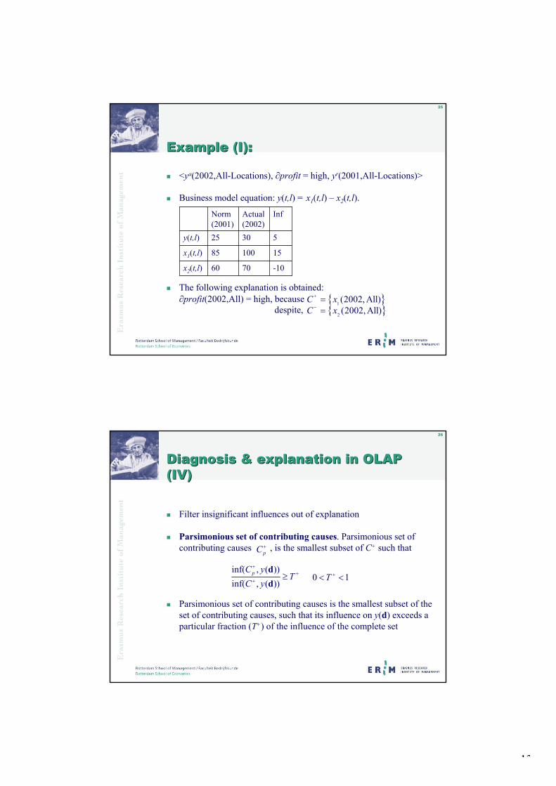
13

25

ExampleExample (I):(I):

<ya(2002,All-Locations), profit = high, yr(2001,All-Locations)>

Business model equation: y(t,l) = x1(t,l) – x2(t,l).

The following explanation is obtained:profit(2002,All) = high, because

despite,

-107060x2(t,l)

1510085x1(t,l)

53025y(t,l)

InfActual(2002)

Norm(2001)

1 (2002, All)C x2 (2002, All)C x

26

Diagnosis & Diagnosis & explanationexplanation in OLAP in OLAP (IV)(IV)

Filter insignificant influences out of explanation

Parsimonious set of contributing causes. Parsimonious set of contributing causes , is the smallest subset of C+ such that

Parsimonious set of contributing causes is the smallest subset of the set of contributing causes, such that its influence on y(d) exceeds a particular fraction (T+) of the influence of the complete set

pC

inf( , ( ))inf( , ( ))

pC yT

C ydd

0 1T

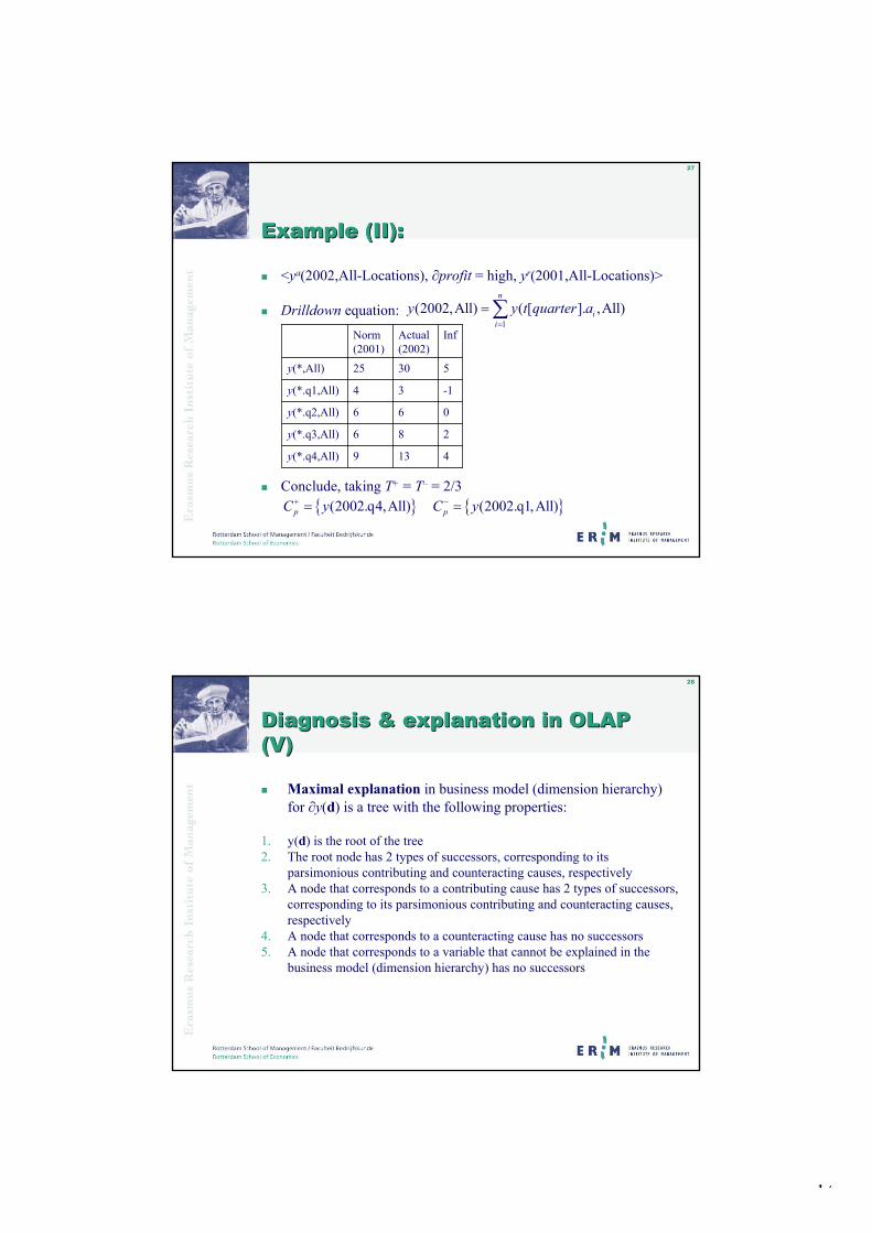
14

27

ExampleExample (II):(II):

<ya(2002,All-Locations), profit = high, yr(2001,All-Locations)>

Drilldown equation:

Conclude, taking T+ = T– = 2/3

1(2002,All) ( [ ]. ,All)

n

ii

y y t quarter a

066y(*.q2,All)

286y(*.q3,All)

4139y(*.q4,All)

-134y(*.q1,All)

53025y(*,All)

InfActual(2002)

Norm (2001)

(2002.q4,All)pC y (2002.q1,All)pC y

28

Diagnosis & Diagnosis & explanationexplanation in OLAP in OLAP (V)(V)

Maximal explanation in business model (dimension hierarchy) for y(d) is a tree with the following properties:

1. y(d) is the root of the tree2. The root node has 2 types of successors, corresponding to its

parsimonious contributing and counteracting causes, respectively3. A node that corresponds to a contributing cause has 2 types of successors,

corresponding to its parsimonious contributing and counteracting causes, respectively

4. A node that corresponds to a counteracting cause has no successors5. A node that corresponds to a variable that cannot be explained in the

business model (dimension hierarchy) has no successors

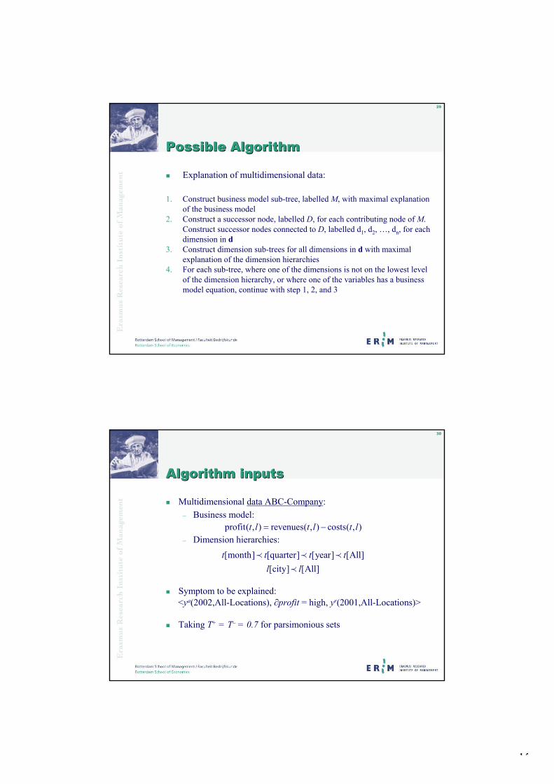
15

29

Possible AlgorithmPossible Algorithm

Explanation of multidimensional data:

1. Construct business model sub-tree, labelled M, with maximal explanation of the business model

2. Construct a successor node, labelled D, for each contributing node of M.Construct successor nodes connected to D, labelled d1, d2, …, dn, for each dimension in d

3. Construct dimension sub-trees for all dimensions in d with maximal explanation of the dimension hierarchies

4. For each sub-tree, where one of the dimensions is not on the lowest levelof the dimension hierarchy, or where one of the variables has a business model equation, continue with step 1, 2, and 3

30

Algorithm inputsAlgorithm inputs

Multidimensional data ABC-Company:– Business model:

– Dimension hierarchies:

Symptom to be explained:<ya(2002,All-Locations), profit = high, yr(2001,All-Locations)>

Taking T+ = T– = 0.7 for parsimonious sets

profit( , ) revenues( , ) costs( , )t l t l t l

[month] [quarter] [year] [All]t t t t[city] [All]l l

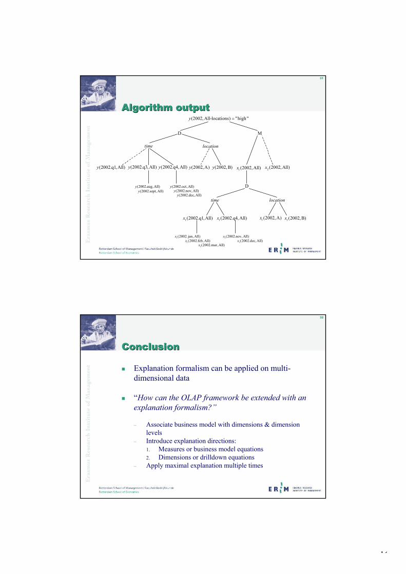
16

31

AlgorithmAlgorithm outputoutput(2002, All-locations) "high"y

1(2002,All)x 2 (2002, All)x(2002.q3, All)y (2002.q4, All)y

(2002.dec,All)y

D

time

location

M

(2002,A)y (2002, B)y

D

time

1(2002, A)x 1 (2002, B)x1 (2002.q1,All)x 1(2002.q4, All)x

1(2002.nov, All)x1(2002.dec, All)x

location

(2002.q1, All)y

(2002.oct,All)y(2002.nov,All)y

(2002.aug,All)y(2002.sept, All)y

1(2002.jan, All)x1(2002.feb, All)x

1(2002.mar, All)x

32

ConclusionConclusion

Explanation formalism can be applied on multi-dimensional data

“How can the OLAP framework be extended with an explanation formalism?”

– Associate business model with dimensions & dimension levels

– Introduce explanation directions:1. Measures or business model equations2. Dimensions or drilldown equations

– Apply maximal explanation multiple times

17

33

ReferencesReferences

H.A.M. Daniels, A.J. Feelders, “Theory and methodology: a general model for automated business diagnosis”, European Journal of Operational Research, 130: 623-637, (2001).

T. Thalhammer, M. Schrefl, M. Hohania: “Active data warehouses: complementing OLAP with analysis rules”, Data & Knowledge engineering, 39, 241-269, (2001).

E. Thompsen: “OLAP Solutions: Building muldimensional Information Systems”, (1997).

Software: Cognos Powerplay (Cognos.com), MS Excel (Add-in), MS Analysis Services, Business Objects, MicroStrategy, etc.

Page 1



Second Workshop on Smart Adaptive Systems in Finance

Intelligent Risk Analysis & Management

Second Workshop on Smart Adaptive Systems in Finance

Intelligent Risk Analysis & Management



Learning Points W. Hallerbach

There are only stupid mistakes, but the impact can be very large and hazardous

Risk is unexpected (but also ubiquitous?)

Deviations from expectations

Chinese wisdom: danger – opportunity

Dealing with complexity (e.g. of new instruments)

„ ... approximate answers to precise problems and not precise answers to approximate problems ...“

adapting to actual situation (e.g. risk attitudes, framing)

There are only stupid mistakes, but the impact can be very large and hazardous

Risk is unexpected (but also ubiquitous?)

Deviations from expectations

Chinese wisdom: danger – opportunity

Dealing with complexity (e.g. of new instruments)

„ ... approximate answers to precise problems and not precise answers to approximate problems ...“

adapting to actual situation (e.g. risk attitudes, framing)

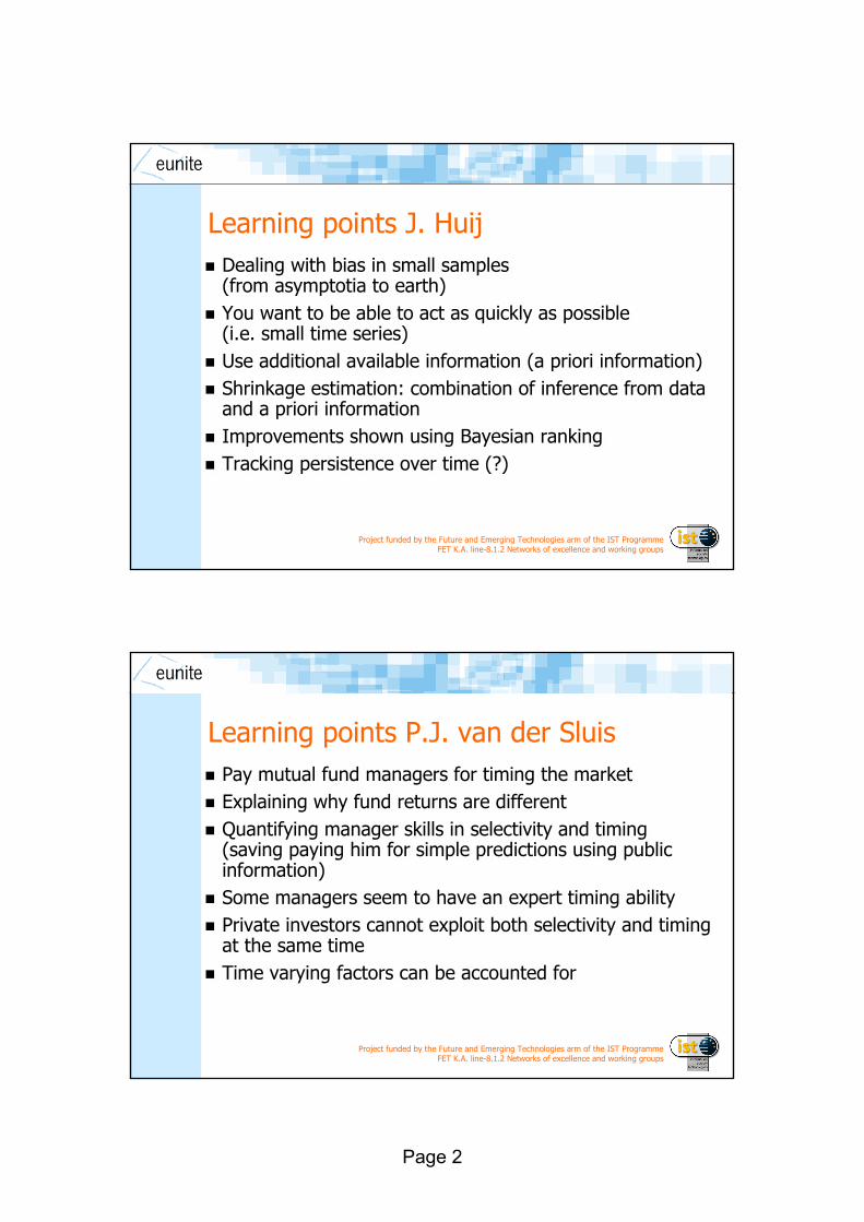
Page 2



Learning points J. HuijDealing with bias in small samples (from asymptotia to earth)You want to be able to act as quickly as possible(i.e. small time series)Use additional available information (a priori information)Shrinkage estimation: combination of inference from data and a priori informationImprovements shown using Bayesian rankingTracking persistence over time (?)

Dealing with bias in small samples (from asymptotia to earth)You want to be able to act as quickly as possible(i.e. small time series)Use additional available information (a priori information)Shrinkage estimation: combination of inference from data and a priori informationImprovements shown using Bayesian rankingTracking persistence over time (?)



Learning points P.J. van der SluisPay mutual fund managers for timing the marketExplaining why fund returns are differentQuantifying manager skills in selectivity and timing(saving paying him for simple predictions using public information)Some managers seem to have an expert timing abilityPrivate investors cannot exploit both selectivity and timing at the same timeTime varying factors can be accounted for

Pay mutual fund managers for timing the marketExplaining why fund returns are differentQuantifying manager skills in selectivity and timing(saving paying him for simple predictions using public information)Some managers seem to have an expert timing abilityPrivate investors cannot exploit both selectivity and timing at the same timeTime varying factors can be accounted for

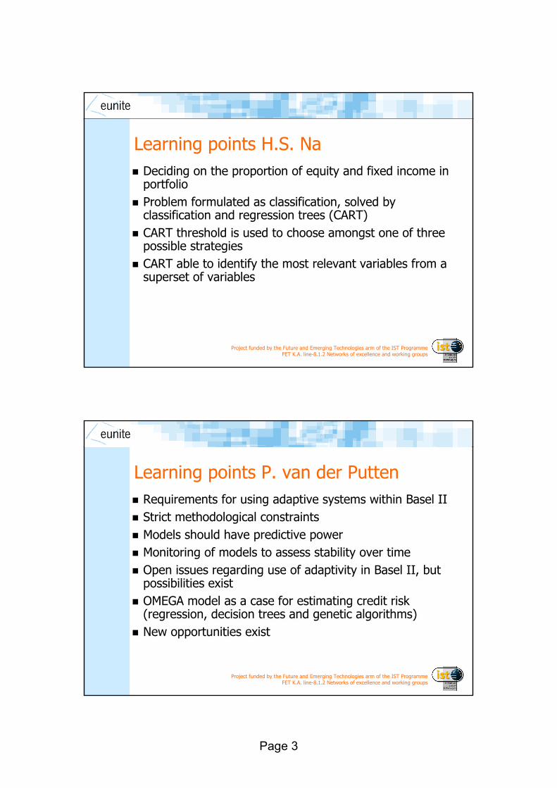
Page 3



Learning points H.S. Na Deciding on the proportion of equity and fixed income in portfolioProblem formulated as classification, solved by classification and regression trees (CART)CART threshold is used to choose amongst one of three possible strategiesCART able to identify the most relevant variables from a superset of variables

Deciding on the proportion of equity and fixed income in portfolioProblem formulated as classification, solved by classification and regression trees (CART)CART threshold is used to choose amongst one of three possible strategiesCART able to identify the most relevant variables from a superset of variables



Learning points P. van der PuttenRequirements for using adaptive systems within Basel IIStrict methodological constraintsModels should have predictive power Monitoring of models to assess stability over timeOpen issues regarding use of adaptivity in Basel II, but possibilities existOMEGA model as a case for estimating credit risk(regression, decision trees and genetic algorithms)New opportunities exist

Requirements for using adaptive systems within Basel IIStrict methodological constraintsModels should have predictive power Monitoring of models to assess stability over timeOpen issues regarding use of adaptivity in Basel II, but possibilities existOMEGA model as a case for estimating credit risk(regression, decision trees and genetic algorithms)New opportunities exist

Page 4



Learning points L. MirandaEconomic capital for operational risk

– Quantitative information– Qualitative information

Qualitative information to modify quantitative predictions: it captures uncertainty due to knowledge imperfectionSAS contribute to deal with qualitative information

– Fuzzy logic to process linguistic and subjective knowledge– Linguistic description of model in addition to numeric predictive

power

More possibilities for soft computing and SAS due to knowledge intensive nature of operational risk

Economic capital for operational risk– Quantitative information– Qualitative information

Qualitative information to modify quantitative predictions: it captures uncertainty due to knowledge imperfectionSAS contribute to deal with qualitative information

– Fuzzy logic to process linguistic and subjective knowledge– Linguistic description of model in addition to numeric predictive

power

More possibilities for soft computing and SAS due to knowledge intensive nature of operational risk



Learning points G. DikosAdaptive decision support system that will have a commercial valueEquilibrium models for real and auxiliary marketsAdaptive systems could also be interesting as a future route for econometric models, attractive because of their simple parameterizationDesign of smart systems should not exclude using statistical modelsWill SAS bring break-through models in economics?Use theoretical models if you have a good one!

Adaptive decision support system that will have a commercial valueEquilibrium models for real and auxiliary marketsAdaptive systems could also be interesting as a future route for econometric models, attractive because of their simple parameterizationDesign of smart systems should not exclude using statistical modelsWill SAS bring break-through models in economics?Use theoretical models if you have a good one!

Page 5



Learning points E. CaronExtend OLAP with explanation formalismBusiness models associated with dimensions and dimension levelsExplanation directionsBasic framework onto which smart adaptive systems and methodologies could be built

– E.g. linguistic explanation capability

Extend OLAP with explanation formalismBusiness models associated with dimensions and dimension levelsExplanation directionsBasic framework onto which smart adaptive systems and methodologies could be built

– E.g. linguistic explanation capability



ConclusionsMaking models more inline with reality

– Better predictions– Improved explanation– Stronger decision support

There is nothing more practical than a good theoryPotential for smart adaptive systems, and much has to be researched stillGrowth from academic research into actual business cases

Making models more inline with reality– Better predictions– Improved explanation– Stronger decision support

There is nothing more practical than a good theoryPotential for smart adaptive systems, and much has to be researched stillGrowth from academic research into actual business cases