Proc. MICCAI workshop: Challenge on Liver Ultrasound Tracking

Proc. MICCAI workshop: Challenge on Liver Ultrasound Tracking

37

tracking solutions at high frame rates at the cost of reduced image quality anda smaller field of view. Additionally ultrasound imaging allows isotropic imageresolution in 3D and does not suffer from intra-frame motion.

Development of fast tracking methods on continuous ultrasound imaging iscurrently subject of research. State-of the-art methods for motion estimationin 2D and 3D suggest ultrasonic speckle tracking [4], or rigid [5] and non-rigidregistration [6]. More sophisticated approaches make use of statistically validatedmotion models [7] [8] or combine scale-adaptive block-matching algorithms withlearning-based techniques [9].

To achieve on-line motion compensation, it is necessary that the methodswork in real-time, i.e. faster than the incoming imaging frame rate. Additionally,it is necessary for some setups to compensate for latencies that might occur dur-ing ultrasound image streaming [10] [11] and mechanical latencies [12] [13] (pages1 to 4). For this reason, it will be useful to combine the tracking method withadditional prediction algorithms to obtain a glimpse into the near future.

In this paper we present two algorithms for fast and robust tracking, one ofthem capable to cope with frame rates of up to 25 Hz, and combine the trackingresults with a prediction method that allows a prediction horizon of 200 ms.Additionally, we introduce a real-time capable smoothing of the tracked point’strajectory using polynomial fitting, which improves the prediction.

2 Methods

2.1 Datasets

The CLUST challenge provided 23 2D US sequences of the liver of volunteertest subjects under free breathing with a duration of 120 to 580 seconds. Thesequences have a temporal resolution of 11-25 Hz and isotropic in-plane resolu-tion of 0.35-0.71 mm. Two of the sequences come with 2 respectively 3 manuallylabeled ground-truth annotations for approximately 10% of the frames as a train-ing set. A total of 54 points had to be tracked in the test-set where only theinitial position was given.

The 3D datasets consist of 11 sequences with a duration of 5.8 to 27 seconds.The temporal resolution varies from 6 to 24 Hz depending on the sequence. Thespatial resolution is not necessarily isotropic for all sequences and is in a rangeof 0.3 mm up to 1.2 mm. 21 annotations have been provided for the first frameas the test-set and 4 points as training data.

2.2 2D Motion Tracking using Dense Optical Flow

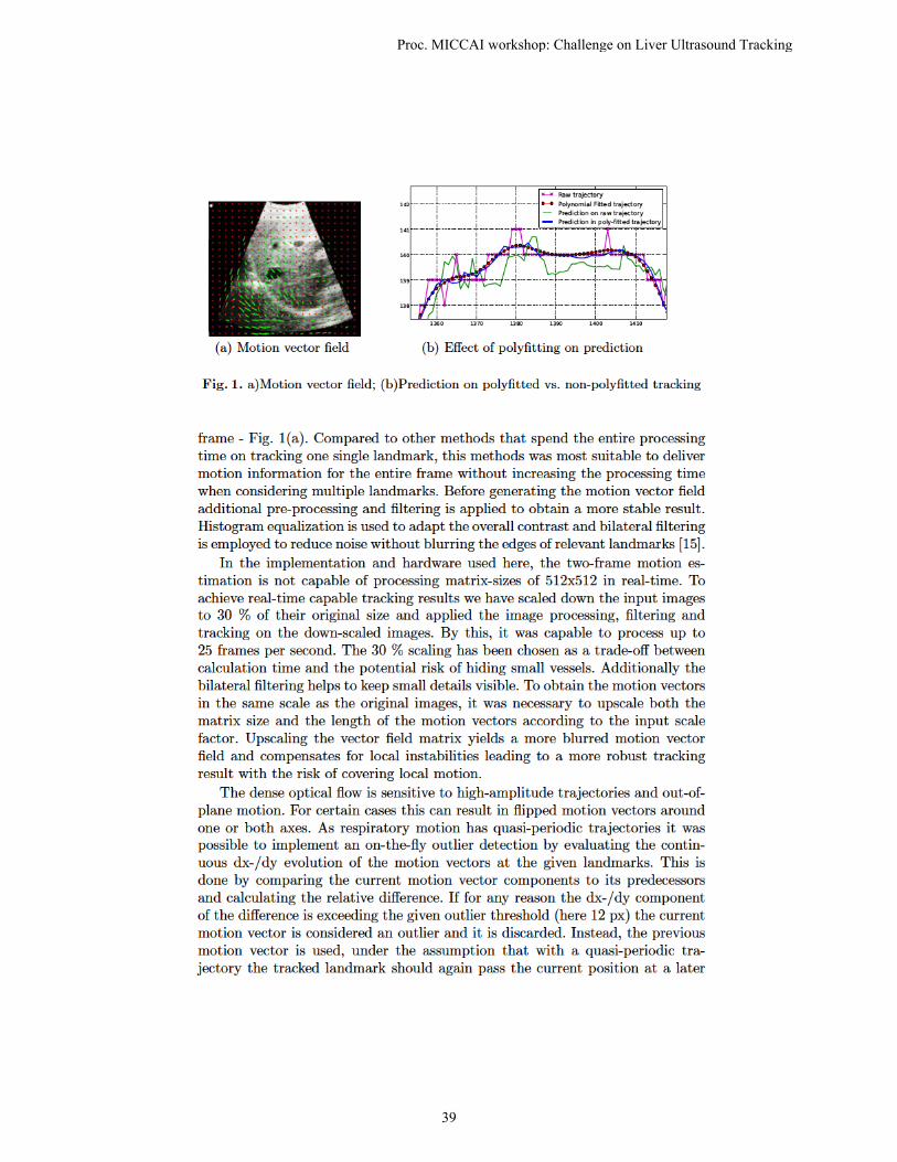
The first 2D motion tracking method is using a two-frame motion estimationbased on G. Farnebaeck’s polynomial expansion [14] and has originally beenadapted by us for motion tracking in MR images. We use the first frame as areference and apply the tracking on each subsequent frame in comparison to thereference. The result of this operation is a dense motion vector field for the entire


38


39

time. When plotting the trajectories over time the detected outliers appear assensor-clipping. By applying real-time capable polynomial fitting (1st order) tothe outlier-filtered trajectories, it is possible to compensate for the clipping. Toachieve non-linearity on a 1st order polynomial fit, the fit is done on overlappingsegments with a constant window-size (number of samples) and then averagingthe accumulated fits for each sample. Another aim of the polynomial fitting isto provide smoother input for the prediction described in 2.5. The polynomialfitting tends to under-estimate the motion for the true extreme values but ap-pears to correctly over-estimate the motion for the samples where the outlierdetection causes the clipping of the trajectory component.

2.3 2D Motion Tracking on GPU

This heuristic procedure has several parameters that were tuned on the labeled2D data provided for training. Preprocessing: the images were resized for speedsuch that the width is 160 pixels. Most of the features to track were vessels(roughly a black round area surrounded by a whiter tissue boundary), for whichwe try to get automatically the cross-section radius (r), in the first image. Forcases that look differently, a default r = 5 pixels is used. The scale of the image isincreased and the estimation repeated until r ≥ 2. Each tracked point is treatedindependently, possibly even using the same images resized at a different scale.A mask is computed containing all pixels that change in a dataset, which corre-sponds to a device-specific viewport. It can be extracted from previous sessionsand reused, or extracted from the first image automatically under mild assump-tions. Registration: a quadratic patch with the edge size of 6r (to include theregion of interest and a local neighborhood) is then extracted from the scaledfirst image and used as reference. From 3000 random patches with uniformlyrandom variations of size (±10%) and random skewness (0 . . . 40%), distributedover the whole field of the current frame, the most similar is computed on GPU.The similarity function used is the minimum of the correlation coefficients ofthe entire patch and of the left/right/top/bottom parts with the correspondingparts of the reference. A second local search is then performed. This looks forthe best variation (same ranges as above) of the patch found in the first pass,after a reduction of the edge’s size to 80%. To avoid the flaws of this simplesimilarity function, a different one is used to evaluate further the best matchingpatch found - the correlation coefficient of the polar coordinates representationof the central inscribed disc of the patch. For both similarity functions the maskwas taken into account in an attempt to improve the tracking behavior next tothe boundary of the valid area. This is achieved by ignoring the computations ofthe pixels known to be outside of the valid area. Postprocessing: in our firstGPU submission we have filtered the raw position guesses produced by the GPUregistration using a simple jump detection, using as threshold 3r. For a secondGPU-based submission, we used the same input but a more refined filtering thatlooked both for sudden jumps in position and for sudden variations in similar-ity. The thresholds used were continuously automatically adjusted, assuming anormal distribution of the frame-to-frame distances and of the matching quality


40

(thresholds set to 3 times the empirical standard variance of the populationscorresponding to frames where the tracking is believed to be good).

2.4 3D Motion Tracking

The same method as in 2.2 has been used for the 3D tracking, which is here in facta 2.5D approach. This was done by applying the tracking on the two orthogonalslices that intersect at the given annotation after rotating the volumes such thatthe first 2D coordinate lies in the XY-plane and the second one in the ZY-plane(depending on the alignment of the input data). This yields two separate trackingresults per frame. As both slices share the Y-axis in 3D space, the tracking resultsfor this redundant axis have been averaged for both results and we use the X- andZ-components independently as the final 3D position. As the orthogonal slicesare fixed in their Z-coordinate, the method is sensitive to out-of-plane motionof the landmark to track. To compensate for out-of-plane motion it is necessaryto adjust the Z-coordinate for one slice according to the X-component of themotion vector from the orthogonal plane (left as future work).

2.5 Prediction

For the 2D motion vectors, we tested a robust on-line prediction method thatwe developed for respiratory motion compensation (tested previously on theCyberknife respiratory motion dataset3) after a preprocessing described in [13]at page 100, set here for predicting the position of the point of interest 200 ms intothe future. As there is only one signal, like there was for the Cyberknife data, theproblem is one of pure auto-regression. The algorithm we used is a linear auto-regression (AR). More precisely, we employed iterated stable linear regression (3iterations, elimination of outliers at quantile 0.95). The auto-regression modelwas updated once per second, using only data not older than one minute. We usedan order that corresponds to 4.5 seconds at 20 Hz sampling rate. From the historywindow, the AR model was built to depend only on the values {T + dt; dt ∈{0,−1,−2,−3,−5,−8,−13,−21,−34,−55,−89}}, a Fibonacci progression thatstops at 4.5 s into the past (for 20 Hz sampling rate) from the last known value T .The accuracy we obtained on the Cyberknife database using the Fibonacci auto-regression delays were comparable to the ones obtained using the full historywindow, but the speed was much increased by a factor of about 10. Less trainingdata had to be collected, as there were less parameters to estimate, therefore theprediction could start earlier. As the current implementation of the predictioninvolves a learning phase of 30 seconds, we did not try to use this prediction forthe 3D tracking due to the insufficient length of the datasets.

2.6 Software Tools and hardware

The methods described in 2.2 were implemented using the Mevislab software,Python, OpenCV and Numpy. The actual tracking and timing measurement has

3available at http://signals.rob.uni-luebeck.de/index.php/Signals @ ROB, by courtesy of Dr.Kevin Cleary and Dr. Sonja Dieterich


41

been executed on a Intel Core i7-4770k with 32 GB RAM. The GPU method hasbeen implemented in Matlab (CPU Intel Xeon E5540, 24 GB RAM) and CUDA(GPU Nvidia Geforce GTS 450).

3 Results

Tracking Results from Dense Optical Flow: given the fact that focusedultrasound treatment usually involves ablation of a safety margin around thetumor [16], the dense optical flow tracking turned out to work with the pre-cision required for surgery despite the reduced resolution due to down-scalingthe images. The mean tracking error (MTE) for the entire test-set of 54 pointsis 1.82 ± 2.37 mm. Only 5 out of 54 points yielded poor results with a meanerror above 3 mm. The high-deviation results can be explained by out-of-planemotion causing the tracked landmark to change its shape or if the landmarkis close to the border of the field of view in combination with high amplitudemotion. This occasionally causes the motion vectors to flip around one axis forcertain cases. The polynomial fitting has almost no impact on the overall out-come (1.82 ± 2.34 mm) and mostly helps to marginally improve results thatalready have low deviation. The average calculation time for all points is 40 msdepending on the amount of scaling.

GPU Tracking Results: the more refined, self-tuning outliers detectionproduced better results than the simple threshold detection. The mean trackingerror it produced was 1.55±2.78 mm for one 2D subset (outperforming the denseoptical flow based method) and 2.40± 2.78 mm for the second one. The averageprocessing time per frame was 250 ms (179 ms without using the advancedoutliers detection), conditioned by the speed of the GPU.

3D Tracking Results: as the 3D tracking is lacking a Z-coordinate ad-justment the results are suffering from out-of-plane motion. The MTE is 5.24±4.34 mm for all 21 points across different datasets. One data subset has a sig-nificantly higher error of 7.61 mm. This can be explained by the lower andanisotropic voxel-resolution. As the tracking is performed on two orthogonalslices the average processing time per frame of 60.68 ms is slightly higher thanin the 2D datasets but still below the 3D images’ frame-rate (real-time) exceptfor one data subset with temporal resolution of 24 Hz.

Prediction Results: the prediction has been executed on both the polyfit-ted and non-poly-fitted dense optical flow results, however only the prediction onthe non-polyfitted results has been submitted for evaluation. The MAE for theprediction results is 2.04±2.36 mm. Given that polynomial fitting has no impacton the quality of the dense optical flow tracking (see 3) it was possible to deter-mine the difference (RMS) of the prediction on the polyfitted and non-polyfittedresults. While the prediction on the non-polyfitted tracking results reproducesthe high-frequency motion and leads to reduced precision of the prediction, the


42

polynomial fitted trajectories decrease the RMS deviation for the prediction by65 % for all points - Fig. 1(b)4.

4 Discussion and Conclusion

As the result of the Dense Optical Flow tracking is a motion vector field for theentire image, multiple points/landmarks can be tracked in parallel without anyadditional processing time. If the expected trajectory of the landmark is knownin advance, it is possible to apply the dense optical flow on a small patch ofthe input image. This can significantly reduce the processing time and allowsto omit the scaling operation to preserve all details in the region of interest.To improve the 3D tracking, it is planned to adjust the slices’ Z-coordinateaccording to the orthogonal X-motion vector. As the outliers from the trackingcan be detected on-the-fly, there is a chance to improve the prediction by takingthe outlier-indicators into account to reduce the influence of those samples onthe prediction. For 2D tracking it is essential to minimize out-of-plane motionby proper alignment of the FOV orthogonal to the dominant axis of motion.

The GPU used is more than three years old and underpowered in comparisonto the latest ones, which limited our options in compromising between the speedand the quality of the optimization. The speed of the GPU tracking is completelyscalable and can be much higher (reaching real-time capabilities on preliminarytests with a more modern graphic card, Quadro K5000).

We have shown in this paper the results of two tracking algorithms in combi-nation with auto-regressive prediction. While both tracking methods work withthe precision required for surgery [16], there is a small advantage in precisionfor the GPU tracking. The dense optical flow tracking has an advantage in itscapability to cope with high imaging frame rates and the additional benefit ofbeing able to track multiple landmarks in the same image without any additionalprocessing time. Even though the GPU tracking is not capable of handling thehigh frame rate of US imaging, it might be useful to combine it with the denseoptical flow tracking and potentially predict intermediate positions from infre-quent updates from both tracking methods. The runtime overhead for both thepolynomial fitting and the prediction is negligible in comparison to the pro-cessing time for the tracking. Interestingly the polynomial fitting has significantinfluence on the prediction results. As the prediction results for the polynomialfitted tracking are almost indistinguishable from the polyfitted tracking results,the performance of the prediction solely depends on the the quality of its inputdata.

References

1. J. R. McClelland, D. J. Hawkes, T. Schaeffter, and A. P. King. Respiratory motionmodels: A review. Medical image analysis, 17(1):19–42, 2013.

4The MAE for the prediction on the polyfitted tracking is 1.85 ± 2.36 mm. This result is not partof the CLUST competition, being sent for evaluation after the challenge ended – but before thetrue labels for the test set to be provided to the participants.


43

2. JE. Kennedy, F. Wu, GR. Ter Haar, FV. Gleeson, RR. Phillips, MR. Middleton,and D. Cranston. High-intensity focused ultrasound for the treatment of livertumours. Ultrasonics, 42(1):931–935, 2004.

3. C. Grozea, D. Lubke, F. Dingeldey, M. Schiewe, J. Gerhardt, C. Schumann, andJ. Hirsch. ESWT-tracking organs during focused ultrasound surgery. In MachineLearning for Signal Processing (MLSP), 2012 IEEE International Workshop on,pages 1–6. IEEE, 2012.

4. M. Pernot, M. Tanter, and M. Fink. 3D real-time motion correction inhigh-intensity focused ultrasound therapy. Ultrasound in medicine & biology,30(9):1239–1249, 2004.

5. R. J. Schneider, D. P. Perrin, N. V. Vasilyev, G. R. Marx, P. J. del Nido, and R. D.Howe. Real-time image-based rigid registration of three-dimensional ultrasound.Medical image analysis, 16(2):402–414, 2012.

6. S. Vijayan, S. Klein, E.F. Hofstad, F. Lindseth, B. Ystgaard, and T. Lango. Valida-tion of a non-rigid registration method for motion compensation in 4D ultrasoundof the liver. In Biomedical Imaging (ISBI), 2013 IEEE 10th International Sympo-sium on, pages 792–795, April 2013.

7. E.-J. Rijkhorst, I. Rivens, G. ter Haar, D. Hawkes, and D. Barratt. Effects of Respi-ratory Liver Motion on Heating for Gated and Model-Based Motion-CompensatedHigh-Intensity Focused Ultrasound Ablation. In Medical Image Computing andComputer-Assisted Intervention MICCAI 2011, volume 6891 of Lecture Notes inComputer Science, pages 605–612. Springer Berlin Heidelberg, 2011.

8. F. Preiswerk, V. De Luca, P. Arnold, Z. Celicanin, L. Petrusca, C. Tanner, O. Bieri,R. Salomir, and P. C. Cattin. Model-guided respiratory organ motion predictionof the liver from 2D ultrasound. Medical image analysis, 18(5):740–751, 2014.

9. V. De Luca, M. Tschannen, G. Szekely, and C. Tanner. A Learning-Based Approachfor Fast and Robust Vessel Tracking in Long Ultrasound Sequences. In MedicalImage Computing and Computer-Assisted Intervention MICCAI 2013, volume8149 of LNCS, pages 518–525. Springer Berlin Heidelberg, 2013.

10. J. Schwaab, M. Prall, C. Sarti, R. Kaderka, C. Bert, C. Kurz, K. Parodi,M. Gunther, and J. Jenne. Ultrasound tracking for intra-fractional motion com-pensation in radiation therapy. Physica Medica, 2014.

11. M. Prall, R. Kaderka, N. Saito, C. Graeff, C. Bert, M. Durante, K. Parodi,J. Schwaab, C. Sarti, and J. Jenne. Ion beam tracking using ultrasound motiondetection. Medical physics, 41(4):041708, 2014.

12. R. Durichen, T. Wissel, and A. Schweikard. Optimized order estimation for autore-gressive models to predict respiratory motion. International Journal of ComputerAssisted Radiology and Surgery, 8(6):1037–1042, 2013.

13. F. Ernst. Compensating for Quasi-periodic Motion in Robotic Radiosurgery.Springer, New York, December 2011.

14. G. Farneback. Two-frame motion estimation based on polynomial expansion. InImage Analysis, pages 363–370. Springer, 2003.

15. C. Tomasi and R. Manduchi. Bilateral filtering for gray and color images. InComputer Vision, Sixth International Conference on, pages 839–846. IEEE, 1998.

16. Y.-S Kim, H. Trillaud, H. Rhim, H. K. Lim, W. Mali, M. Voogt, J. Barkhausen,T. Eckey, M. O. Kohler, B. Keserci, et al. MR Thermometry Analysis of Son-ication Accuracy and Safety Margin of Volumetric MR Imaging–guided High-Intensity Focused Ultrasound Ablation of Symptomatic Uterine Fibroids. Radiol-ogy, 265(2):627–637, 2012.


44

Documents

Proc. MICCAI workshop: Challenge on Liver Ultrasound Tracking