UCRL-JC-128335

PREPRINT

Problems and Solutions (Generalized andFEM) Related to Rapid and Impulsive

Changes for Incompressible Flows

PM. GreshoR.L. Sani

This paper was prepared for submittal to the

10th International Conference on Finite Elements in FluidsTucson, AZ

January 5-8,1998

August 1997

‘fhis is a preprint of a paper intendedfor publication in a journal or proceedings. ‘Since changes may be made before publication, thk preprintis made available withthe understandingthat it will not be cited or reproduced without the permission of the 7

author.

J

DISCLAIMER

This document was prepared as an account of work sponsored by an agency ofthe United States Government. Neither the United States Government nor theUniversity of Californianor any of theiremployees, makes any warranty, expressor implied, or assumes any legal liability or responsibility for the accuracy,completeness, or usefulness of any information, apparatus, product, or processdisclosed, or represents that its use would not infringe privately owned rights.Referenceherein to any specificcommercial product, process, or service by tradename, trademark, manufacturer, or otherwise, does not necessarily constitute orimply its endorsement, recommendation, or favoring by the United StatesGovernment or the University of California. The views and opinions of authorsexpressed herein do not necessarily state or reflect those of the United StatesGovernment or the University of California,and shall not be used for advertisingor product endorsementpurposes.

\

Problems and solutions (generalized and FEM) related to rapidand impulsive changes for incompressible flows

@P.M Gresho

(Lawrence Livermore National Laboratory)

and

R.L. Sani(University of Colorado)

1. INTRODUCTION

We shall be interested in examining so-called‘impulsive’ changes in normal boundary conditions forthe incompressible Navier-Stokes equations, boththeoretically and numerically-via the Galerkin finiteelement method (GFEM) and several time-marchingmethods. We begin by stating two facts:

1.

2.

To

In the ‘strictest’ sense, impulsive (instanta-neous/discontinuous) changes in the normalcomponent of the velocity are illegal in thatthey cause violations of incompressibility, aswell as concomitant unbounded pressure—briefly.

For the very common case in the fluiddynamics literature, the misnomer “impulsivestart from rest” is confusingly employed. It is amisnomer because the true initial condition formost of these analyses and/or simulations ispotential flow-far from a fluid at rest.

help clarify the above issues, we shall alsostudy rapid changes, via driving fimctions for normalvelocity like ( 1– e‘*) for ‘large’ 2-eventuallypermitting A to become unbounded. We focus on but asingle simple and common example: flow past acircular cylinder. The startup-both rapid andimpulsiv~was treated extensively in Gresho and Sani(1997) (hereafter referred to as GS). In this paper, weconcentrate mostly on the opposite case: suddenshutdown (rapid and impulsive) of the flow past thesame cylinder from an IC that was generated in thestartup phase.

For a discussion of some of the previous work inthe startup case, see GS. For the shutdown case, we citethe few with which we are familiac Gresho (1991a)Wang and Dalton (1991), Chang and Maxey (1995),who state, “An impulsively stopped free stream... ismuch different than an impulsively started flowj” and

Mei and Lawrence (1996), who state, “When it issuddenly brought to rest, the wake behind the bodywill continue to move to the right with the wake origintraveling as x - t.”

In the remainder of this paper, we shall ‘analyze’the problems associated with rapid/impulsivechanges-both in the continuum and in the finite h,finite At discrete world in which we are forced to doour computations. For the latter case, we shalldemonstrate the performance of two popular ‘elements’

(Q2EI ~d Q&AI) and the manner in which they (orany other approximate method) behave; viz., dismalfailure at small time-especially for the impulsivecase-with recovery fortunately occurring once the meshnear the cylinder has had time to ‘recognize’ thesituation and respond to the severe challenge. Anotherproblem, somewhat surprising, is the discovery that the‘stable’-for-Stokes-flow element ( Q2P_1) is less stable(bigger wiggles) for potential flow than the Q@element that is deemed by some to be unstable (againfor Stokes flow).

2. THEORY

We shall ‘sneak up’ on impulsive changes as fol-lows: Find g and P flom

and

with

@+l@+vP=vv2gatv.g=o~Q, (l%b)

U=EO e-*+4-e-*) ‘n ‘> ‘2)

~=go at r=O (3)

that satisfies both

V.go=O in Q (4)

and fl.~o=~.~o on r. 9 (5)

where A is a parameter that will be allowed to becomearbitrarily huge-with A + co defining our impulsivechange. (Actually, the Dirichlet BC of(2) will only beapplied on a portion of r; the remaining BC’s will bepresented later.)

The pressure Poisson equation (PPE) impliedby (l),

)(6)V2p=V. (vV2g-g. Vg in 42

an~ from (1) and (2), it’s implied (Neumann) BC (see,e.g., Gresho and Sani [1987], GS),

aP/& = ~ o[Vvzg-g oVg-ik/a]

(=rJ.vv2g-&.vg

)

-fl.(X1-Eo)h-k on r, (7)

are especially important to understand. Hopefully it isobvious (at least after due reflection) that for 1sufficiently large, and t sut%ciently, small the pressuresatisfies

V2P~0 in Q

with dP/dns -fl. (U1 - yo) k-ti on ~,

i.e., the acceleration BC dominates the problem.

Remarks: 1) For impulsive (or rapid) startsrest, go=~ and E. =(J.

(8)

(9)

from

2) For impulsive (or rapid) stops,yl=Q.

Noting that (8) and (9) are ‘solved’ by

p= -.-$ae-~, (lo)

where @is the potential function satisfying

V2@=0 in fl (11)

and */~=a-(Y1 -yo) on r, (12)

2

permits the realization that an impulsive change viaDirichlet BC changes in the normal velocity is actuallynothing more than a potential flow ‘adjustment’ +vortex sheet; i.e. for A + co our ‘new’ IBVP is simplythis: Find ~ and P with the modzjied IC and BC,

y=~o– V@ in Q and U=yl on r; (13%b)

and we note the presence of a vortex sheet on r since~.g=~.~l on r but ~.y=Z.~o-~-V@#f.E1 justoff of the surface. For A large-but-finite, this is of courseonly an approximation (still for small time) to the trueIBVP given by (1) through (5).

It is also worthwhile pointing out the followingprojection connection for A+ =.: The solution of (1 l)-(13) can also be derived as follows: (1) make a stepchange inthe BCfiom n.u=n. wo to n.u=n. wl;—— —-— —(2) call the resulting non~s~enoidal velocity & (i.e.ii=~o in $,2 with fl.~=~.~l (#EgO) on r; (3)kis is realized via (i) solve V2@= V. ~ in S2 with6i#/& =g. (ij-g)=O on r, where V“ij is to beinterpreted as a Dirac delta function on r; (4) computeg =&- V@, which will give the same result as Eqn.(13). (Admittedly, the ‘continuous’ approach, witha + DOat the end, is somewhat more intuitivelyacceptable-but the equivalence is important.)

Note ilom (9) that A + ~ puts a version of theDirac delta function, a so-called generalized fi.mction,onthe boundary:

6(2) = se-h, (14)

which satisfies ~~~(t)dt=l and ~~.f(r)i$(t~t ‘~(o)for A+ 00, and causes dP/& to become unbounded.

Note too that this same limit causes both aninfinite pressure and a violation of incompressibility—both briefly-the latter a consequence of a step changediscontinuity in the normal velocity at the boundary

(E” U=g”Yo at t =0 but E.u=u.x1 for t= O+). Itis this violation that has caused us to state thatimpulsive changes are “illegal” for incompressible flow(cf. Gresho 1991b, GS). Arbitrarily large 1!s are quitepermissible, of course. Here, however, we shall ‘softenup’ and take the broader view that impulsive changesare just as legitimate as are generalized solutions.

Consider now the application of the above theoryto a particular case: rapid startup of flow past a circularcylinder (radius a) in an unbounded domain. We fwsttreat the inviscid (potential flow) case, as the resultinganalytical solutions provide some useful insight.

For this case, the following solution (in polarcoordinates) is easily obtained

~,=(’-e-w (15)

whcxe @= wl(r+ a2/r)cos 6. (16)

Also,

P[ = –@e-fi + Ppot“(l-’-hr

(17)

gives the concomitant pressure, where the potentialpressure is

‘Pot=w’cos’+’18)For the limiting case of an impulsive st@ A + co andwe get

24, = H~(t)v@ (19)

and PI= -w(t) + ~2(t) Ppot, (20)

where we ‘interpret’ Hi(t) as Heaviside step finc-tions— Hi(0)= O ~d Hi(t)= 1 for t >0. Note thatd(t) generates the potential flow and Hi(t) maintainsit, which is our interpretation of an (ideal) impulsivestart from rest.

For the viscous (no-slip) case, we do not know theexact solution, but in GS we have developed (withmuch help from A.C. Hindmarsh, to whom we remainindebted) the following useful approximation (model),valid within the boundary la er (BL) and close to the

Pcylinde~ i.e., for r – a cc 4vt and r – a <e a:

where TaC= 1/2 is the acceleration time constant andD(.) is Dawson’s integral, which behaves like so:

~Y)~Y for Y<<l, ~Y)=~Y for Y>>l, with~y) attaining its only maximum ofD(- 0.92)= 0.54. The corresponding pressure is givenby

For both the rapid start and the impulsive start, weemphasize that D(O) = O—and also note that

~~)/&~~~ for A+=(and t> O), whichlatter result makes our model agree with previousimpulsive start theoretical analyses [e.g.,. Wang(1968), Collins and Dennis (1973), Bar-Lev and Yang(1975)] in that both viscous and pressure contributionsto the drag coefilcient, for small time, can be shown tobe (see GS for details)

c~=%J:w3giving, for At cc 1,

which corresponds to the accelerationwithin the BL, while for k>> 1 we get

(23)

(24)

phase of flow

(25)

which accounts for the deceleration within the BL—andis the result referred to above in the impulsive startliterature (none of whom treat the accelerating phase),and we emphasize that even for the limiting case(A+co), (25) only applies for t>O; C] =C~ =0 att = O. The final contribution to the drag coefficientcomes from the acceleration portion of the transientpressure field and can be derived as

(26)

using (17) and (22).The total drag coefficient is, of course,

CD. C;+ C;+ C;, (27)

and we note that PPOt in (17) contributes naught toCD, per d’Alembert. Thus, for A arbitrarily large, CDstarts at an arbitrarily large value owing to C: (theDirac function, in the limit) and for t >0 but small,goes like @ in which both the viscous componentand the pressure component are ‘caused’ by the no-slipBC, the pressure part needing to utilize V. g = O toclearly see its viscous ‘roots’; see GS for details.

Finally we note, for d -+ CO,that there exists anear-vortex sheet on the cylinder at t = 0+. For a‘classic’ impulsive start, (A= -) if such a thing exists,the IC is potential flow for r> a with a true vortex

3

sheet on r = a caused by suddenly imposing the no-slip BC. We are in fact somewhat ‘bothered’ by such adefinition because it is quite misleading; the flow is notatrestat t=O.

3. NUMERICS

So much for theory. How does a CFD code deal withthe above issues, which clearly must lead to someserious numerical challenges for large 2 and, as weshall show, to total failure at small tfor A = co? Webegin by returning to the analytical pressure solution,(22), and note its satisfaction of the following BC onthe cylinder (for 2 sufficiently large that thecontribution from PPOtis negligible):

which behaves like (and causes the viscous part of the

)

pressure to also behave like) O(AJ for small

)t(fi <c 1) and like 0(1/~ for ‘large’ tAt>> 1). Butthe ‘numerical’ version o this Neumann BC, derivedin GS, is rather different:

aP = VMjCos e

z ~- a2 (a/h-4T-e-*) ’29)

where the second term might be argued to at leastapproximate the physics (accelerating potential flow)outside the BL. (h is the distance tlom the cylinder tothe first node point in the fluid.) But the fwst andspurious term, which necessarily dominates for all casesof interest ( h C< a ) does not—and the physics withinthe BL is completely lost. Not only does this‘numerical BC’ fail to describe reality, it clearlydiverges and leads to unbounded pressure for h + O!By requiring that the far field PPE BC,

‘k dominate the spurious one indP/dr = -w, COS6.ae(29) the following (ap~roximate) “window of non-believability; can be derived (see GS for details):

where

ahTact%— < t < TMTB,

mm(30)

(31)

is called the Minimum Time of Believability—andactually came about while analyzing the limiting caseA= ~, the impulsive start. For A = ~, the numericalsolution can not be believed for t < tMTB, whereas forthe rapid startup (finite A) the numerical solution ismostly believable for t < tac &(ah/vraC ) because the

acceleration-dominated phase is not so difficult tocompute successfully. It is not believable when (30)applies, and both types of startup are believable/usefulwhen t > ZMTB,because the mesh can now ‘follow’ theviscous diffusion process because the BL now containsat least 1 node point. Of course, for the finite A case, agood mesh design would preclude the left inequality in(30) via

~MTB= h2/4v = ZaCln(ah/vrm) (32)

which, for given v and ZaC, can be solved for h-andwe point out the bad news that Zac + O+ h + O.Even when (32) is satisfie& however, the details of thesolution within the BL cannot be captured by the finitemesh for t < ~~B; e.g., in GS is shown the followingfor the ‘numerical version’ of C;:

CL=2zvAt/wlh (33)

fm t c rMTB, vis-a-vis the correct result, given in (23)-(25).

Enough on the ‘theory’ of the spatial numerics.Now we address the fact that, just as we cannotcompute with h = O, so too can we not time-integrateour resulting differential-algebraic equations (DAE’s)exactly—we must also deal with finite At. The GFEMapproximation to (1)-(5) is (cf., e.g., GS for details)

Mu+ N(u)u + CP = –Ku + f (t) (34a)

and CTU= g(t) (34b)

with, when well-posed (in the ‘strict’ sense), an IC UOthat satisfies

C%. = g(o) = go . (35)

These equations also imply the following discretePPE-complete with built in BC’S:

( )CTM-lC P = CTM-l[f – Ku – N(u)u]–j , (36)

and we briefly discuss how two simple ODE methodsbehave when applied to either the index 2 system ofDAB’s given by (34), or the index 1 system ‘defined’ by(34a) and (36); i.e., the PPE replaces (34b) in the index1 formulation. Implicit time integration methods are‘natural for the index 2 formulation whereas the index 1formulation is—after the mass is lumped (which is notalways possible) to convert M (and thus M-l) to a

4

diagonal matrix-amenable to explicit methods; see GSfor details on these issues.

But since we will also show some results using thepenalty method, which method reduces the index on theDAE’s to zero (i.e., to ODE’s), we first brieflysummarize the method the fluid’s incompressibility is‘relaxed’ via the ‘penalty’ equation that relates pressureto incompressibility violation,

QP= A(CTu-g), (37)

where A is the “penalty parameter” and is very large(typically 106-1010 ), and Q is the pressure massmatrix (see, e.g., GS). Inserting (37) into (34a) yieldsthe (very stiff) system of penalty ODE’s:

Mu+ iV(zJ)u= -(K+ACQ-lCT)U

+f(~)+~Q-ldt) . (38)

See Engelman et al. (1982) for discussion related to the“penalty matrix,” B = CQ-lCT, and see GS for adiscussion of the spurious penalty transient-whosebehavior we shall later demonstrate. Note the impliedODE for the pressure [from (37) and (38)]:

~Q~+(CTM-lC)P

= c%-qf-(K+ N(u))u]-g , (39)

vis-a-vis (36), to which (39) ‘returns’ when h>> 1.Fhlly, we apologize for the introduction of a differentparameter with the same symbol (A)—but ‘excuseourselves’ by stating that we will not (but could have)apply the penalty method to the e-fi case.

We now turn to the simplest implicit ODE method;backward Euler applied to the index 2 DAE’s gives

M(Z4.+1-d+ N(un+l)un+lAt

+cPn+l= –KL4n+l+fn+l (40)

and cTun+l = gn+l> (41)

whereas the simplest explicit method (forward Euler,FE) applied to the index 1 DAE’s gives

‘(%+1 - ‘n) + IV(un)UnAt

+cPn = -Kun + fn, (42)

wherein Pn is firstcomputed from

( )CTM-lC Pn = @M-l

[fn -Kun -~(u.)un]-‘n+~gn. (43)

We presented these two well-known methods in detailonly because we need to address the question of howthey ‘perform’ for a step change in velocity thatviolates discrete mass conservation; i.e., for ourimpulsive changes, we are employing IC’S that do notsatis~ CTUO= gO—and we are facing an ill-posedsystem of DAE’s, and one for which an honest.higoroustrapezoid rule (TR) for time integration would‘announce’ the ill-posedness via WIGGLES (ringingvia 2At oscillations; see GS for details).

Thus, starting with BE for n = O we obtain tlom(49 and (41) for the fust time step, with CTul = gl butC’uo+ go,

( )cTu~ -go

CTM-’C Q = At

+CT@[fi - Kul – N(U, )Ul]-y (44)

pressure-where in our case g, = go, for thefor theimpulsive start (or stop). Clearly, when- CT~o #go, itgives P1+ w as At -+ O, thus reflecting the ill-posedness of impulsive changes. It turns out, however,that we can turn this apparent ‘problem’ into a solutionsimply by noting that for sufilciently small & (44)becomes

( )CTM-lC @z CTuO -go, (45)

where @= Atfi, which remains finite for all At,corresponds to the “potential flow adjustment” pre-sented earlier for the continuous case. Thus, for

!’su lcientt’y small At, a single BE step performs theL -projection to the div-free subspace that is associatedwith impulsive changes in normal velocity-a fact thatwe shall put to good use later.

Switching now to the explicit Euler method on thelowered-index DAE’s, we examine the fwst step of FEapplied to (42) and (43) by setting n = O there.Inserting P. from (43) into (42) and operating on theresult with CTM-l gives

5

CTU1–gl = CTUO–go , (46)

a ‘general’ result in the sense that any ODE methodapplied to the index 1 DAE’s will ‘preserve’ thedivergence (see Gresho 1991A GS, for details). Thus,the ‘PPE method’ can not be used to obtain usefidresults when applied to impulsive changes.

Later, we shall demonstrate the above; i.e., we willshow usefid results from BE and discuss the uselessones from FE. We will also show good results forrapid, not impulsive, changes via the e‘~ BC. In GSwe spent lots of time on both rapid and impulsivestartups, both theoretical and via the GFEM and twotime-marching methods, BE and TR, both in the‘smart’ mode (variable At based on physics). Here weshall summarize some of that work, to set the stage forwhat is new herein-viz.,: (1) impulsive and fast

shutdowns, (2) the behavior of several time integrationmethods applied to the ‘illegal’/impulsive case, and (3)the solution to the sudden stop case via the penaltymethod. Thus we shall consider this paper to be anextension of the impulsive (and rapid) start case that isSection 3.19 in GS.

4. NUMERICAL RESULTS FORSTARTUPS

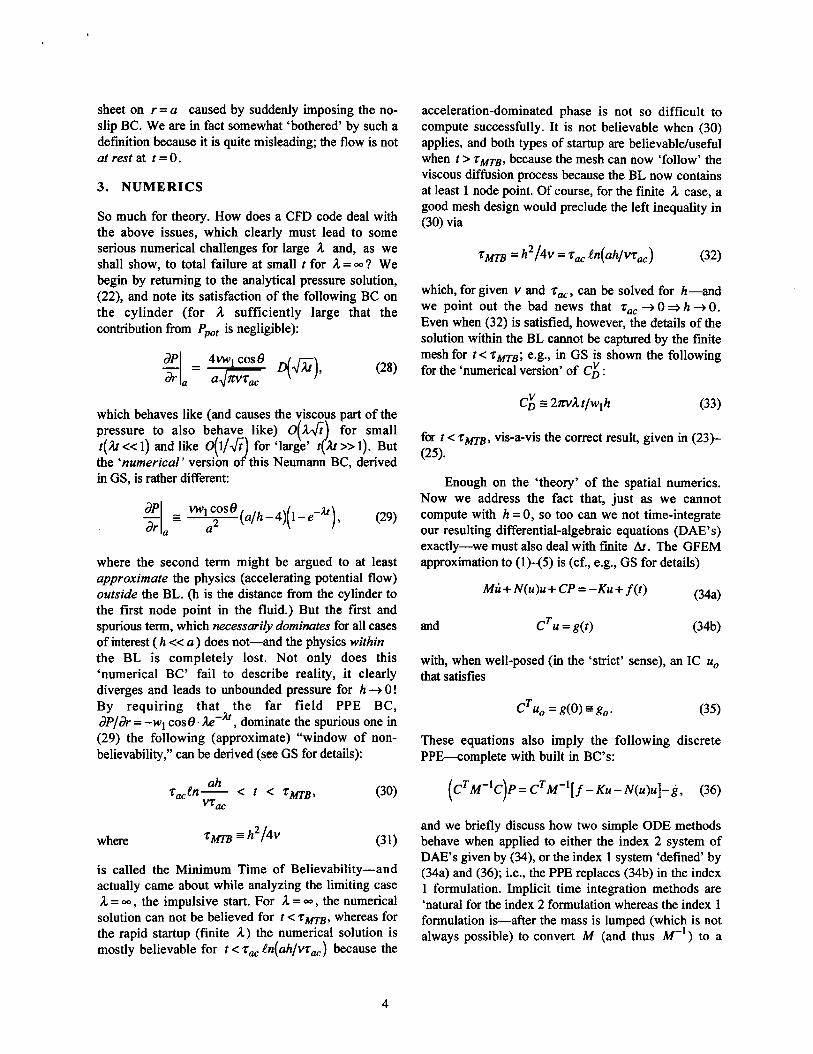
In this section we summarize and paraphrase someof the results in Section 3.19 of GS—partly becausethey are rather interesting and merit a second visit, butmainly to set the stage for the next section—rapidshutdowns. Fig. 1 shows both the domain and themesh employed. The origin of the x – y coordinatesystem is at the center of the unit radius cylinder, andthe domain covers –3<x<3 and ()< Y<2.

(a) The fill domain.

(b) Zoom near the cylinder.

Figure 1: The mesh of 4290 Q2P-1(9/3) elements; 16,965 nodes.

v~/6!x = O) as outflow conditions; y = Q on the

~~:(~-~if ~:~f~s~:~~f~fi:~~~cylinder, and symmetry BC’s were used elsewhere. We

a—the latter case (impulsive) being ‘solved’ by the chose a Reynolds number, Re = 2a wl/v, of 1000technique discussed above of taking one very small BE which translates to v = 0.0002. The mesh shown intime step. Homogeneous natural boun

?

conditions Fig l(a) has 4290 9-node elements, with 16,965(NBC’s) were used at x=3 (v ~ = P and

6

nodes-and we used an equivalent mesh (same numberof nodes) for the 4-node element.

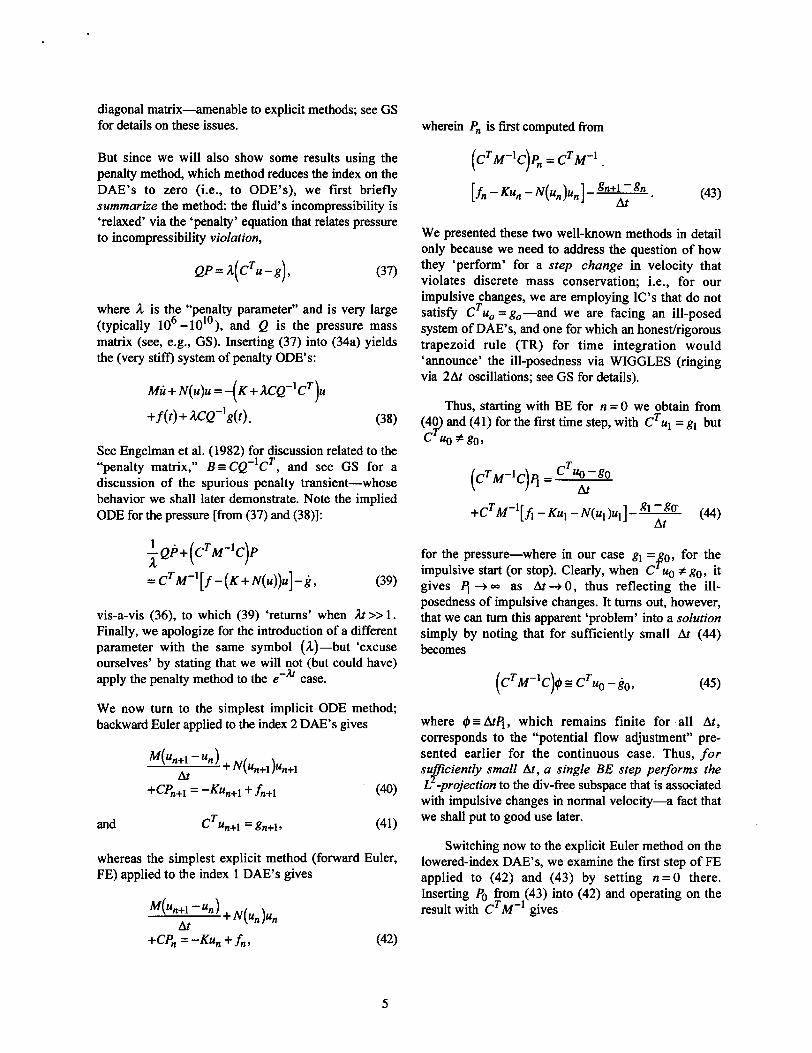
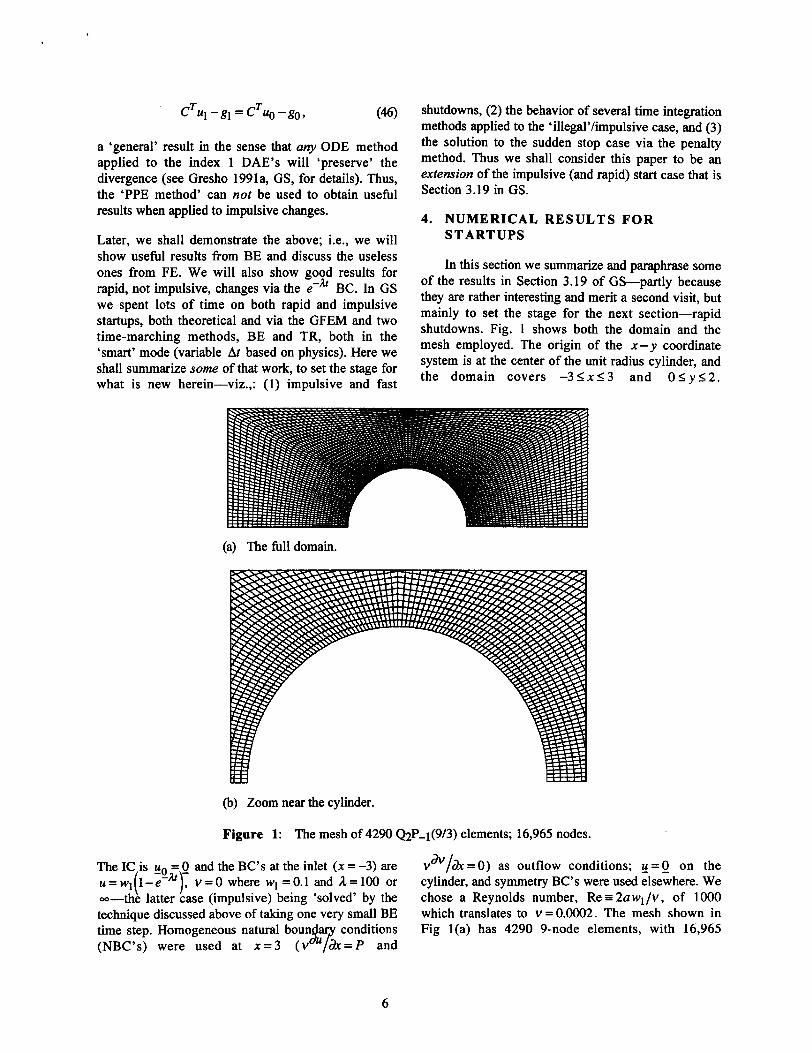
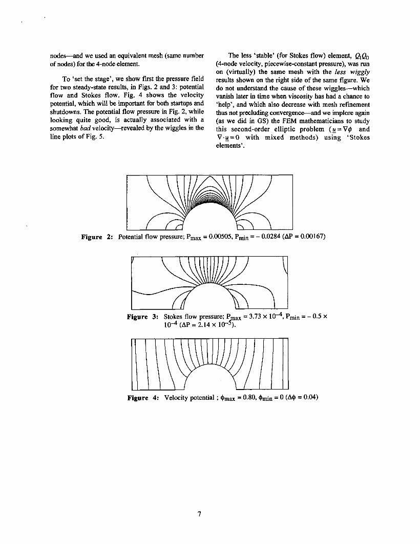
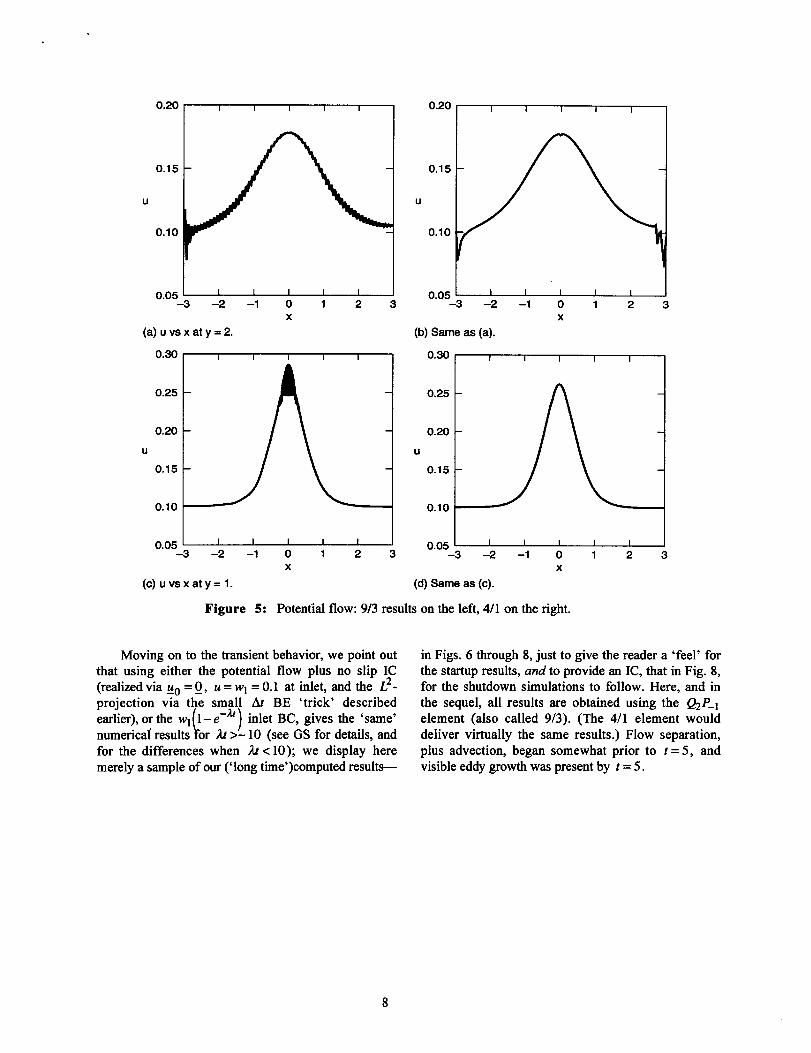
To ‘set the stage’, we show first the pressure fieldfor two steady-state results, in Figs. 2 and 3: potentialflow and Stokes flow. Fig. 4 shows the velocitypotential, which will be important for both startups andshutdowns. The potential flow pressure in Fig. 2, whilelooking quite good, is actually associated with asomewhat bad velocity-revealed by the wiggles in theline plots of Fig. 5.

The less ‘stable’ (for Stokes flow) element, ~~(4-node velocity, piecewise-constant pressure), was nmon (virtually) the same mesh with the less wigglyresults shown on the right side of the same figure. Wedo not understand the cause of these wiggles—whichvanish later in time when viscosity has had a chance to‘help’, and which also decrease with mesh refinementthus not precluding convergence-and we implore again(as we did in GS) the FEM mathematicians to studythis second-order elliptic problem (u= V@ andV. g = O with mixed methods) using ‘Stokeselements’.

Figure 2: Potential flow pressure; Pmax = 0.00505, P~n = -0.0284 (AP = 0.00167)

Figure 3: Stokes flow pressure; Pmm = 3.73 X 104, p~n = – 0.5 x10A (AP = 2.14 X 10-5).

Figure 4: Velocity potential ; $max = 0.80, $~n = O (A41= 0.04)

0“20r————l

0.15 –

u

0.10

“@j ~

–3 –2 –1 o 1 2 3x

(a)uvsxaty=2.

0.30

0.25

0.20

u

0.15

0.10

0.20 I I I I I

0.15 –

u

0.05 I I I I 1-3 –2 –1 o 1 23

x

(b) Same as (a).

0.25

0.20

u

0.15

0.10

“.”5 ~-3 -2 –1 o 1 2 3

x

(c)uvaxaty=l.

““5 ~-3 -2 -1 0 1 2 3

x

(d) Same as (c).

Figure 5: Potential flow: 9/3 results on the left, 4/1 on the right.

Moving onto the transient behavior, we point outthat using either the potential flow plus no slip IC(realized via E.= Q, u= WI= 0.1 at inlet, and the L2-projection via the wn~ll At BE ‘trick’ described

~)earlier), or the WI 1-e inlet BC, gives the ‘same’nmneric~ results or At>- 10 (see GS for details, andfor the differences when At< 10); we display heremerely a sample of our (’long time’)computed results-

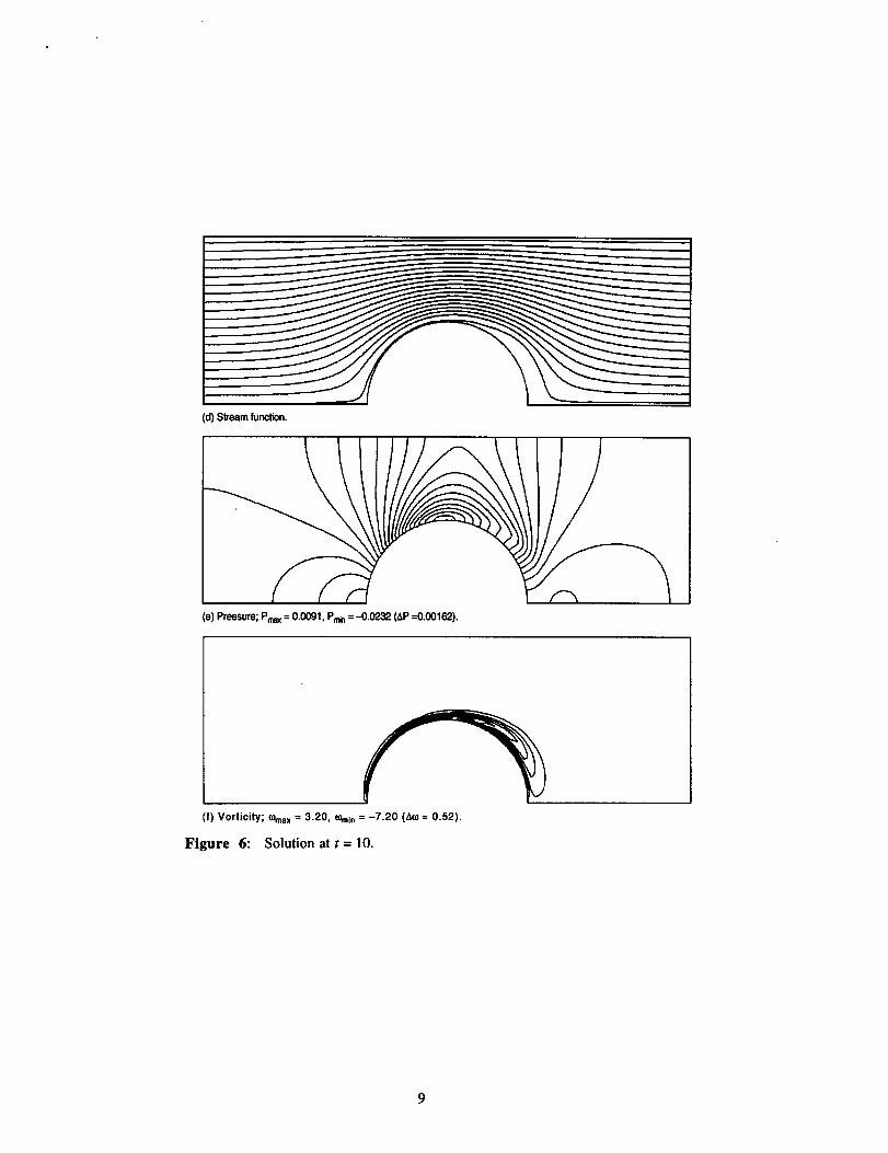
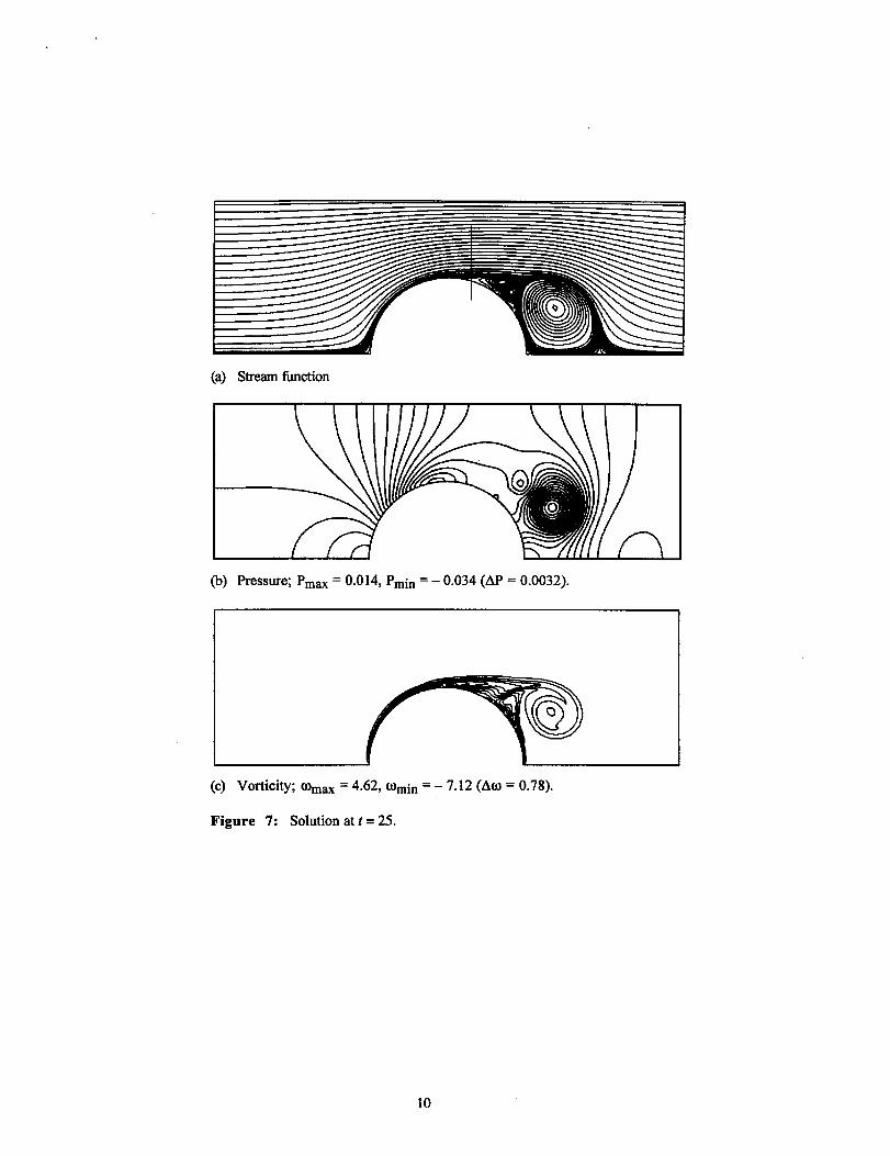
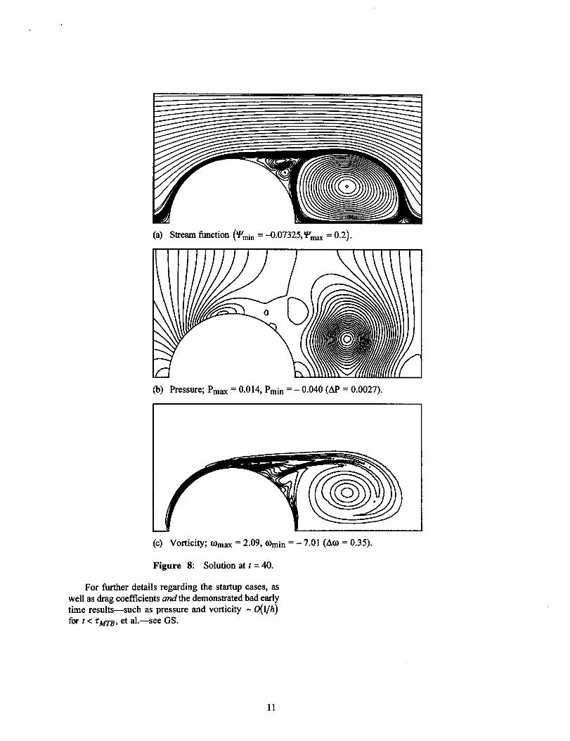
in Figs. 6 through 8, just to give the reader a ‘feel’ forthe startup results, and to provide an IC, that in Fig. 8,for the shutdown simulations to follow. Here, and inthe sequel, all results are obtained using the QP_lelement (also called 9/3). (The 4/1 element woulddeliver virtually the same results.) Flow separation,plus advection, began somewhat prior to t =5, andvisible eddy growth was present by t=5.

8

Es!@(d)Sireemfunction.

(e) PressurqPm = 0.0091, P* = -0.0232 (AP=0.00162).

(f) Vorticity; ~,, = 3.20, ~ln = -7.20 (Mo = 0.52).

Figure 6: Solution at t = 10.

9

(a) Stream fbnction

(b) Pressure; Pmm = 0.014, Pmin = -0.034 (AP = 0.0032).

(c) Vorticity; ~max = 4.62, @rein= -7.12 (ACO= 0.78).

Figure 7: Solution at r = 25.

10

(b) Pressure; Pm= = 0.014, Pmin = -0.040 (AP = 0.0027).

(c) Vorticity; COmW= 2.09, ~min = -7.01 (Am= 0.35).

Figure 8: Solution at t= 40.

For fhrther details regarding the startup cases, aswell as drag coefficients and the demonstrated bad earlytime results—such as pressure and vorticity - 0(1/h)fm tc rm, et al.—see GS.

11

5. NUMERICAL RESULTS FORSHUTDOWNS

We now switch gears and, starting ftom thesolution in Fig. 8, present and discuss some shutdownresults—performed both impulsively and quickly, thelatter via W.= 0.1 and A= 100 at the inlet in (2), withWI= O. We shall also investigate the behavior of thepenalty method. In all cases, we employed slipperyBC’S ( fz = O, a zero pseudo-shear stress-see GS fordetails) except on the cylinder, which had u = Q.

We begin by noting the somewhat remarkable factthat there are rather many seemingly different/disparateways of getting to (virtually) the same place-a resultthat may surprise some. (We hope so!) The “place”they get to, starting from the IC’S discussed above, isthis: the vorticity-perserving potential flow adjustmentplus a new vortex sheet on the cylinder. Here is the listof those that we have discovered thus far-all of whichare virtually independent of Reynolds number, andmost of which are discussed in GS:

1.

2.

3.

4.

5.

6.

7.

An L*-projection.

One very small backward Euler time step.

Exponential decay BC( e‘h) for large k.

The penalty method with accurate timeintegration through the spurious penaltytransient.

The penalty method with inaccurate timeintegration.

One very small FE step on the index 2DAE’s.

The exact (analytical) generalized (anddiscontinuous) solution to the (ostensibly ill-posed) index 2 DAE’s.

Another way to perhaps state these results is this:We have found six different ways to closely

approximate the L2-projection—some which wedemonstrate below.

Also interesting—and somewhat surprising— isthat each of these techniques can generate nearly thesame result (at least for small t) for 3 different sets ofBC’S:

1.

2.

3.

In

Close both ends (slam the door at inlet andoutlet).

Close only the right end.

Close only the left (inlet) end.

the latter two case’s, the “standard”homogeneous (“do nothing”) NBC’S V&/&- p = O

= v&/a , are applied at the open end.

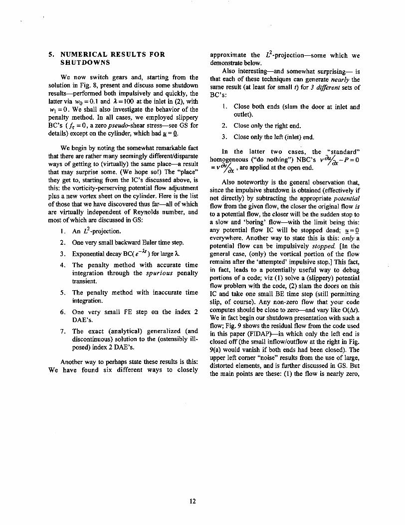
Also noteworthy is the general observation that,since the impulsive shutdown is obtained (effectively ifnot directly) by subtracting the appropriate potentialflow from the given flow, the closer the original flow isto a potential flow, the closer will be the sudden stop toa slow and ‘boring’ flow-with the limit being this:any potential flow IC will be stopped dead; g = Qeverywhere. Another way to state this is this: only apotential flow can be impulsively stopped. [In thegeneral case, (only) the vertical portion of the flowremains afler the ‘attempted’ impulsive stop.] This fact,in fact, leads to a potentially usefid way to debugportions of a code; viz (1) solve a (slippery) potentialflow problem with the code, (2) slam the doors on thisIC and take one small BE time step (still permittingslip, of course). Any non-zero flow that your codecomputes should be close to zero-and vary like O(At).We in fact begin our shutdown presentation with such aflow; Fig. 9 shows the residual flow horn the code usedin this paper (FIDAP)-in which only the left end isclosed off (the small inflow/outflow at the right in Fig.9(a) would vanish if both ends had been closed). Theupper Iefi comer “noise” results flom the use of large,distorted elements, and is further discussed in GS. Butthe main points are these: (1) the flow is nearly zero,

12

(a) Stream fimction ( ~fi = -3.4 x10-9, ~m = 5.6x 10-8)

(b) vorticity (@tin= -5.8x 10-5, ~w = 5.5x 10-5)

Figure 9: Residual flow upon closing the left end on a potential flow.

and (2) the error does scale with At (here At= 5x10-6) unless stated to the contrary, the results to follow are

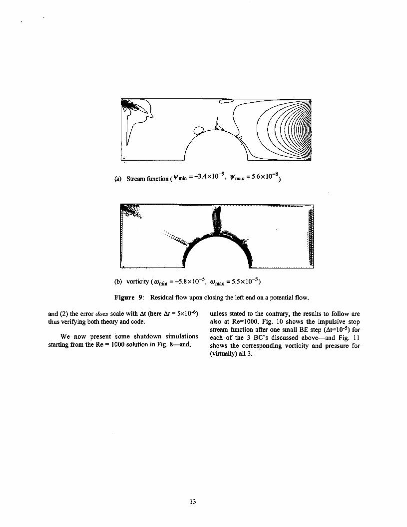
thus verifjhg both theory and code. also at Re= 1000. Fig. 10 shows the impulsive stopstream function after one small BE step (At= 10-5) for

We now present some shutdown simulations each of the 3 BC’S discussed above—and Fig. 11starting from the Re = 1000 solution in Fig. 8—and, shows the corresponding vorticity and pressure for

(virtually) all 3.

13

(a) Both ends closed ( Vti = -0.12293, v~m = 0.00224)

(b) Right end close~ left end open ( Vti = 4.12293, Vmm = 0.00356)

(c) Left end closed, right end open ( IYfin = -0.12589, v- =0.00224)

Figure 10: Flow field (stream function) after 1 small time step via backward Euler.

14

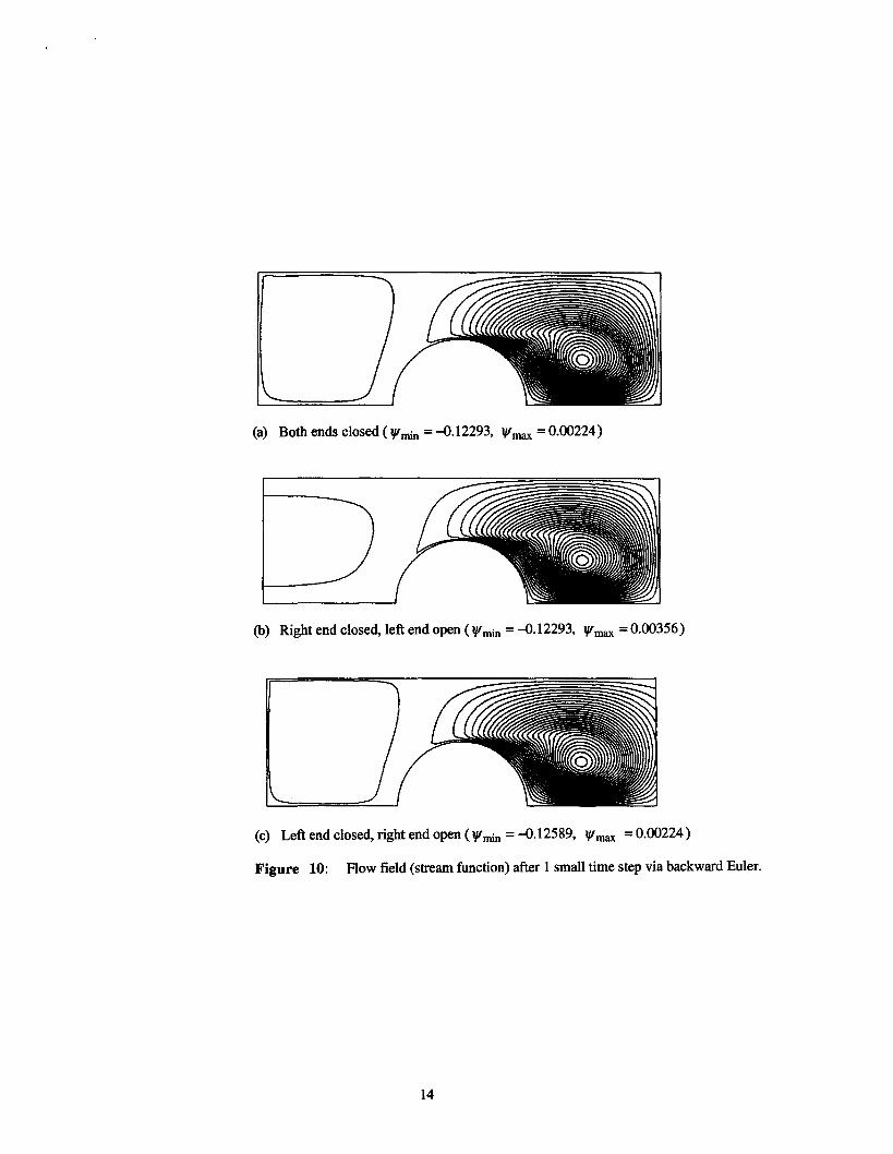
(a) Vorticity ( am = -7.687, O)W = 23.455)

pK%SUre( ~~ = 4.0459, P- = 0.000025)(m

Figure 11: Vorticity and pressure corresponding to Figure 10.

It is obvious that the differences in v are quite small,showing once more the utility of the homogeneousNBC’s as OBC’S. Noteworthy also are the following:(1) The trapped eddy is spinning clockwise, as is thelarge eddy in Fig. 8, and the flow “upstream” isnear-zero-both consequences of subtracting thepotential flow from the viscous flow-and its intensityin the eddy is now greater ( vs -0.125 at the center ofthe eddy, vs. -0.073 prior to the “projection”); (2)The vortex “sheet” has a peak vorticity of +23.5 on thecylinder (a rather far cry from infinity!), whichcorroborates ahnost perfectly with that from the

impulsive start case reported inGS: -23.6; (3) Thevorticity away fkom the vortex sheet is virtually thesame as that in Fig. 8—another consequence of thepotential flow adjustment conservation of vorticity; (4)The pressure is that after 2 time steps, since the Ist stepis a potential field-per Fig. 4 and Eqn. (45).

Next, in Figs. 12 through 15 for the left-end-closedBC, we trace the evolution of the trapped flow-andpoint out that the only “brakes” on the system (besidesviscous dissipation) are those from the no-slip BC onthe cylinder; all other BC’S are frictionless.

15

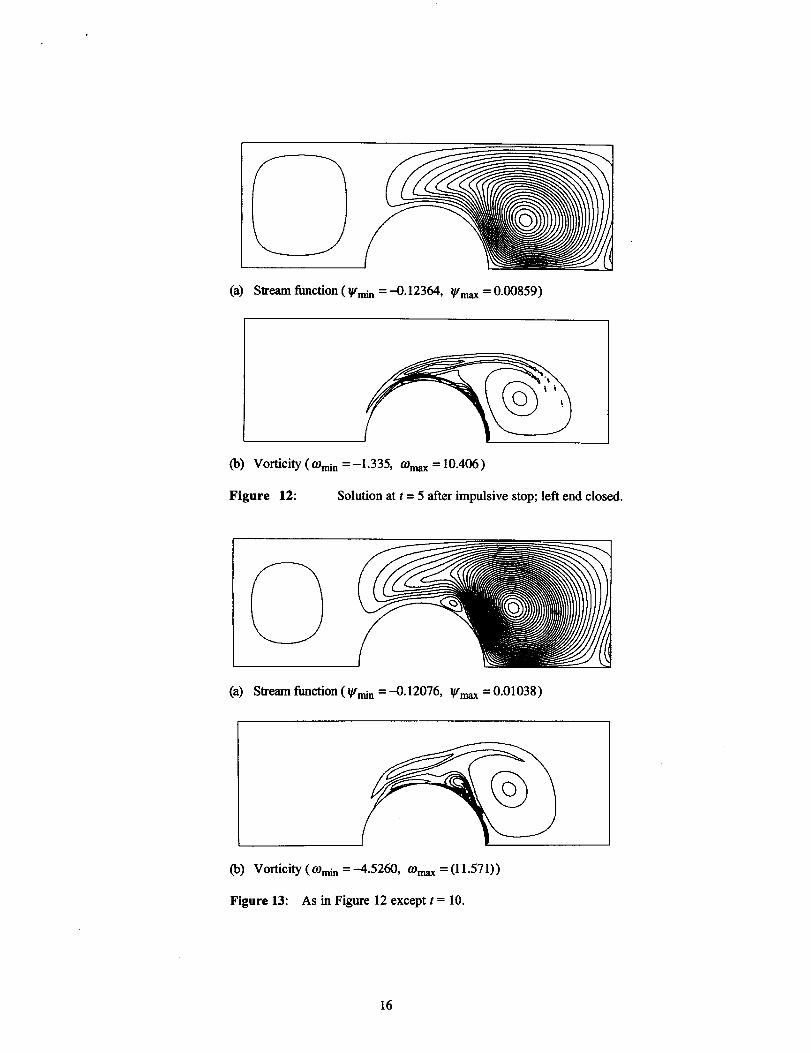
(a) Stream function ( Vti = -0.12364, V-=0.00859)

(b) Vorticity (coti = -1.335, OH= 10.406)

Figure 12: Solution at t= 5 after impulsive stop; left end closed.

(a) Stream iimction ( Vtin = -0.12076, V- = 0.01038)

(b) Vorticity ( @ti = 4.5260, ~-=(1 1.571))

Figure 13: As in Figure 12 except [ = 10.

16

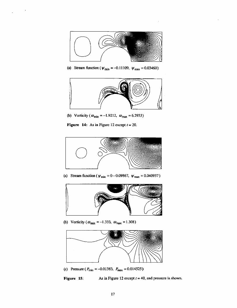
(a) Stream function ( ~fi = -0.11109, y-= 0.03460)

(b)Vorticity ( @ti = -1.9212, CO- = 6.2933)

Figure 14: As in Figure 12 except t = 20.

(a) Stream function ( Vti = 0-0.09867, Vmm = 0.040937 )

(b) Vorticity (mti = -1.333, au= 1.308)

(C) PESSUIW ( Ptin = -0.01383, P-= 0.014525)

Figure 15: As in Figure 12 except t = 40, and preswn‘e is shown.

17

The combination of the initial large vortex and thevortex sheet evolves into a separated flow that spawnsanother eddy (Fig. 13) and yet another (Fig. 14), whilethe large eddy’s center performs another sort ofclockwise rotation on the right side of the cylinder—and these figures can also be ‘interpreted’ as anupstream motion of the original ‘wake’. Although wewent beyond t=40 (Fig. 15) in our simulations, weshow no more because-in fact—the OBC at the rightfinally did cause some poor, nonphysical behavior. Wecould have closed both ends, but chose not to because

we wanted to compare the sudden stop with the e-hshutdown, which BC would be pretty awkward toapply at the right end. Thus, this and all remainingsimulations are for the case of closing off only the left(inlet) boundary.

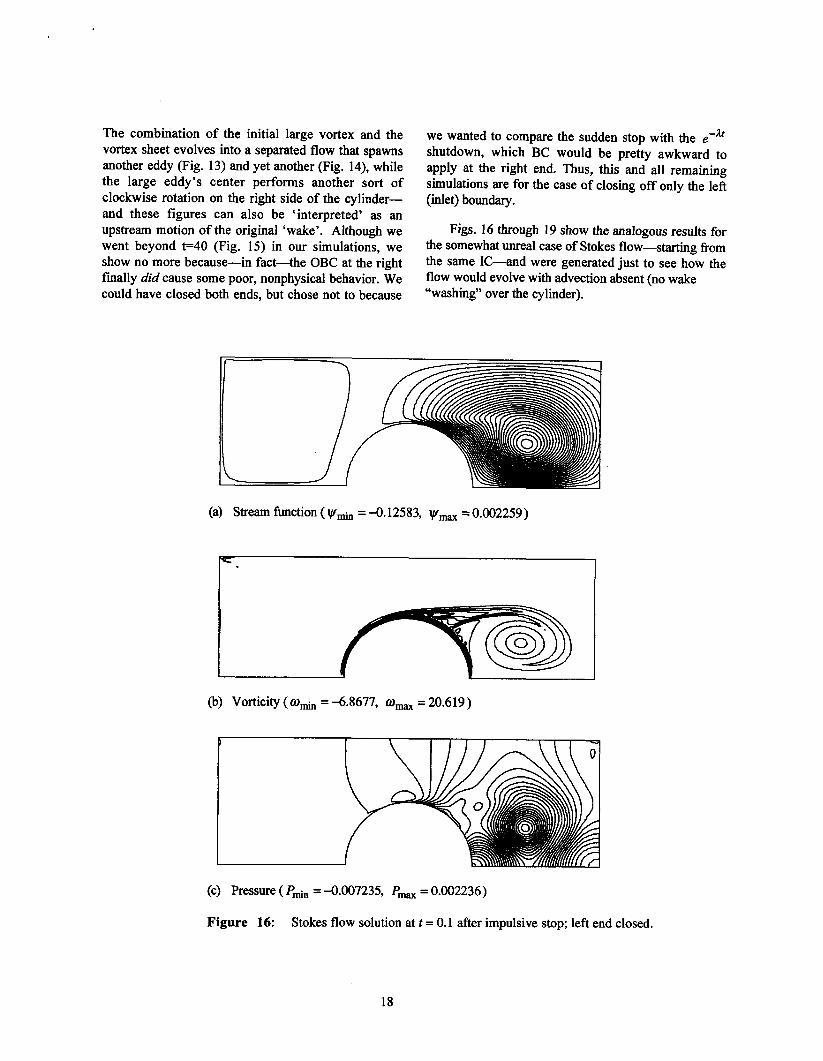
Figs. 16 through 19 show the analogous results forthe somewhat unreal case of Stokes flow-starting fromthe same IC—rmd were generated just to see how theflow would evolve with advection absent (no wake“washing” over the cylinder).

(a) Stream fimction ( Vfi = -0.12583, Vm = 0.002259)

r

(b) Vorticity (coti = -6.8677, mm = 20.619 )

(c) Pressure ( Ptin = -0.007235, P-=0.002236)

Figure 16: Stokes flow solution at t = 0.1 after impulsive stop; left end closed.

18

(a) Stream fiction ( Vtin = 4.12538, V-=0.002336)

v,

(b) Vorticity ( toti = -2.5263, COm = 10.993)

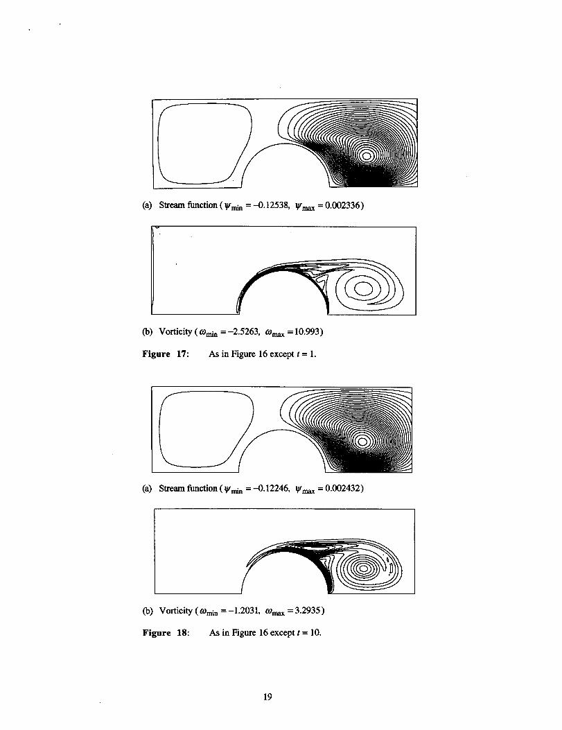
Figure 17: As in Figure 16 except t= 1.

(a) Stream function ( Vfi = -0.12246, ~-= 0.002432)

(b) Vorticity ( mm = -1.2031, O-= 3.2935)

Figure 18: As in Figure 16 except t= 10.

19

(a) Stream function (Vfin=-0.1151 1, Vu= 0.002372)

/

(b) Vorticity ( @ti = -0.99258, co- = 1.5285)

(c) Pressure Pm= -0.000329, P-= 0.000323

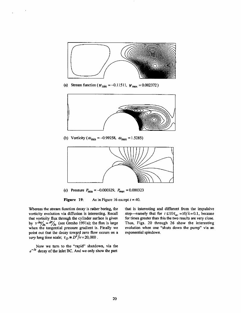
Figure 19: As in Figure 16 except t= 40.

Whereas the stream function decay is rather boring, thevorticity evolution via diffusion is interesting. Recallthat vorticity flux through the cylinder surface is givenby v ao/& = */ti (see Gresho 1991a); the flux is largewhen the tangential pressure gradient is. Finally wepoint out that the decay toward zero flow occurs on ave~ longtime scale; ~D S D2/v=20,000.

Now we turn to the “rapid” shutdown, via thee‘k decay of the inlet BC. And we only show the part

that is interesting and different from the impulsivestop-namely that for t < 10TU =10/A = 0.1, becausefor times greater than this the two results are very close.Thus, Figs. 20 through 26 show the interestingevolution when one “shuts down the pump” via anexponential spindown.

20

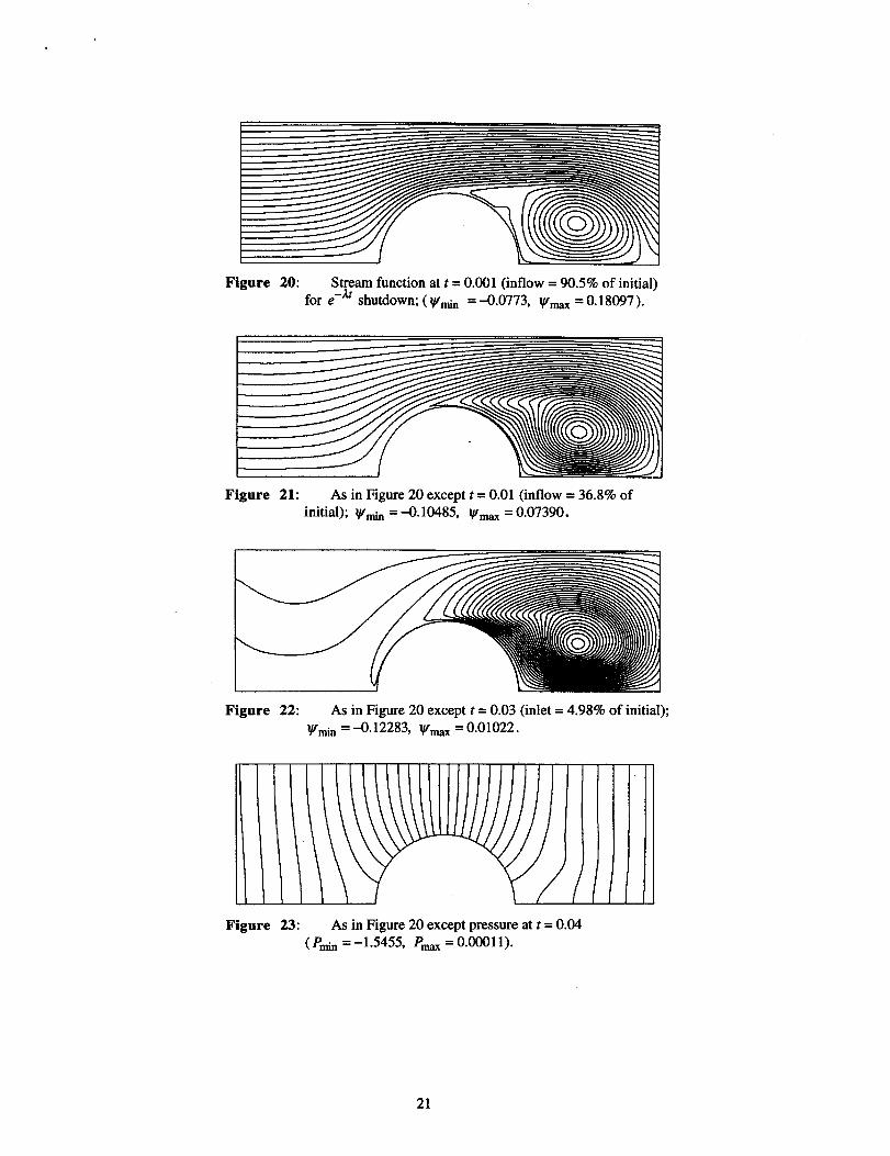
Figure 20: Stream function at t= 0.001 (inflow= 90.5% of initial)for e-k shutdown; ( Vti = -0.0773, I#mm = 0.18097 ).

Figure 21: As in Figure 20 except t = 0.01 (inflow= 36.8% ofinitial); Vti =4.10485, ~- = 0.07390.

Figure 22: As in Figure 20 except t= 0.03 (inlet= 4.98% of initial);—Vti = -0.12283, ~-= 0.01022.

Figure 23: As in Figure 20 except pressure at t = 0.04( Pfi = –1.5455, Pm= O.00011).

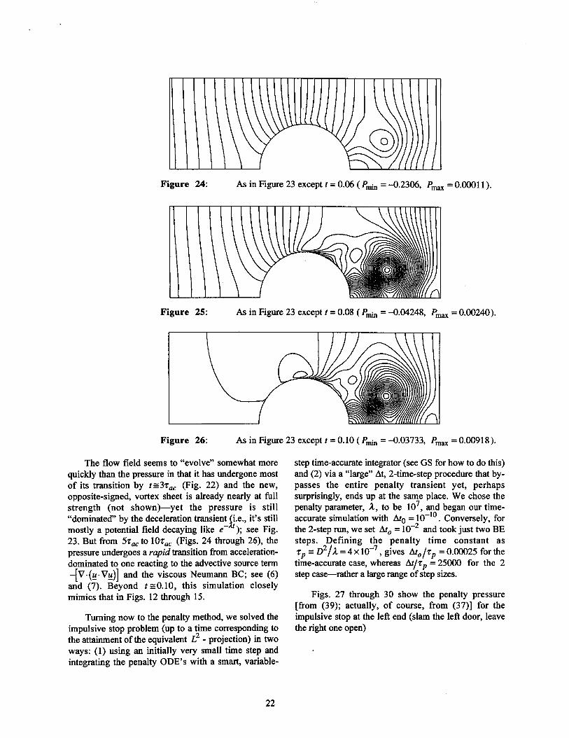
Figure 24: As in Figure 23 except t = 0,06 ( Pti = -0.2306, Pm= 0.00011).

Figure 25: As in Figure 23 except t = 0.08 ( Pti = +.04248, Pm~ = 0.00240).

Figure 26: As in Figure 23 except t = 0.10 ( Pfin = -0.03733, Pmm =0.00918).

The flow field seems to “evolve” somewhat morequickly than the pressure in that it has undergone mostof its transition by t =3taC (Fig. 22) and the new,opposite-signed, vortex sheet is already nearly at fullstrength (not shown)—yet the pressure is still“dominated” by the deceleration transient i.e., it’s still

Lmostly a potential field decaying like e- ); see Fig.23. But from 5zm to 10zaC (Figs. 24 through 26), thepressure undergoes a rapid transition from acceleration-dominated to one reacting to the advective source term-[v.(u.vE)]and the viscous Neumann BC; see (6)and (;). Beyond ts 0.10, this simulation closelymimics that in Figs. 12 through 15.

Turning now to the penalty method, we solved theimpulsive stop problem (up to a time corresponding tothe attainment of the equivalent L2 - projection) in twoways: (1) using an initially very small time step andintegrating the penalty ODE’s with a smart, variable-

22

step time-accurate integrator (see GS for how to do this)and (2) via a “large” At, 2-time-step procedure that by-passes the entire penalty transient yet, perhapssurprisingly, ends up at the same place. We chose thepenalty parameter, 1., to be 107, and began our time-

’10 Conversely, foraccurate simulation with AtO=10 .the 2-step run, we set AfO= 10-2 and took just two BEsteps. Defining the penalty time constant asrP a D2/A = 4 x 10-7, gives ArO/rP = 0.00025 for thetime-accurate case, whereas Af/rP = 25000 for the 2step case-rather a large range of step sizes.

Figs. 27 through 30 show the penalty pressure[horn (39); actually, of course, from (37)] for theimpulsive stop at the left end (slam the left door, leavethe right one open)

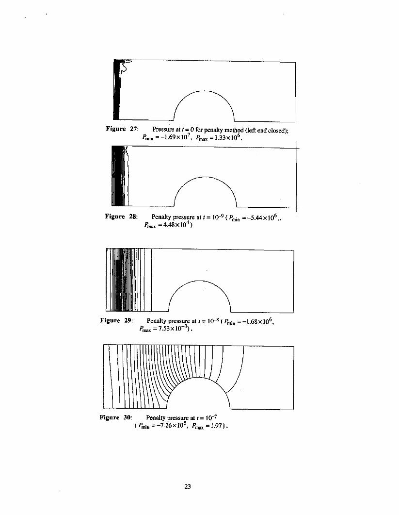
Figure 27: Pressure at t = Ofor penalty method (lefl end closed);Pmin= -1.69x107, PmX = 1.33x106.

Figure 28: Penalty pressure at t = 10-9 ( Pfin = -5.44x 106,.- = 4.48x104)P

I

Figure 29:

!!!JPenalty press~e at t = 10_8( Ptin = –1 .68 x106,

Pm = 7.53x 10-=).

)

Figure 30: Penalty pressure at t = 10_7( P~n = –7.26x105, Pm= 1.97).

23

-.

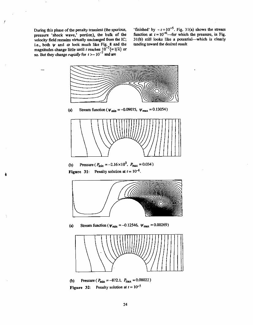
‘5 Fig. 3 l(a) shows the strewDuring this phase of the penalty transient (tie spurious, ‘finished’ by -t= 10‘—for which the pressure, in Fig.pressure ‘shock wave,’ portion), the bulk of the fimction at t= 10

velocity field remains virtually unchanged from the IC; 3 l(b) still looks like a potential-which is clearlyi.e., both v and co look much like Fig. 8 and the tending toward the desired resultmagnitudes change little until r reaches 10-7(= l/1.) orso. But they change rapidly for t>- 10-7 and w

—

(a) Stream thnction ( Vfi = -0.09075, ~-= 0.13054)

(b) Pressure ( Ptin = -2.16x 105, Pm= 0.034)

Figure 31: Penalty solution at t = lti.

(a)

0)

Stream fbnction (v~ = -0.12546, v== 0.00269)

PXIXXW@( P* = -872.1, pm= 0.00022)

Figure 32: Penalty solution at t = 10_5

24

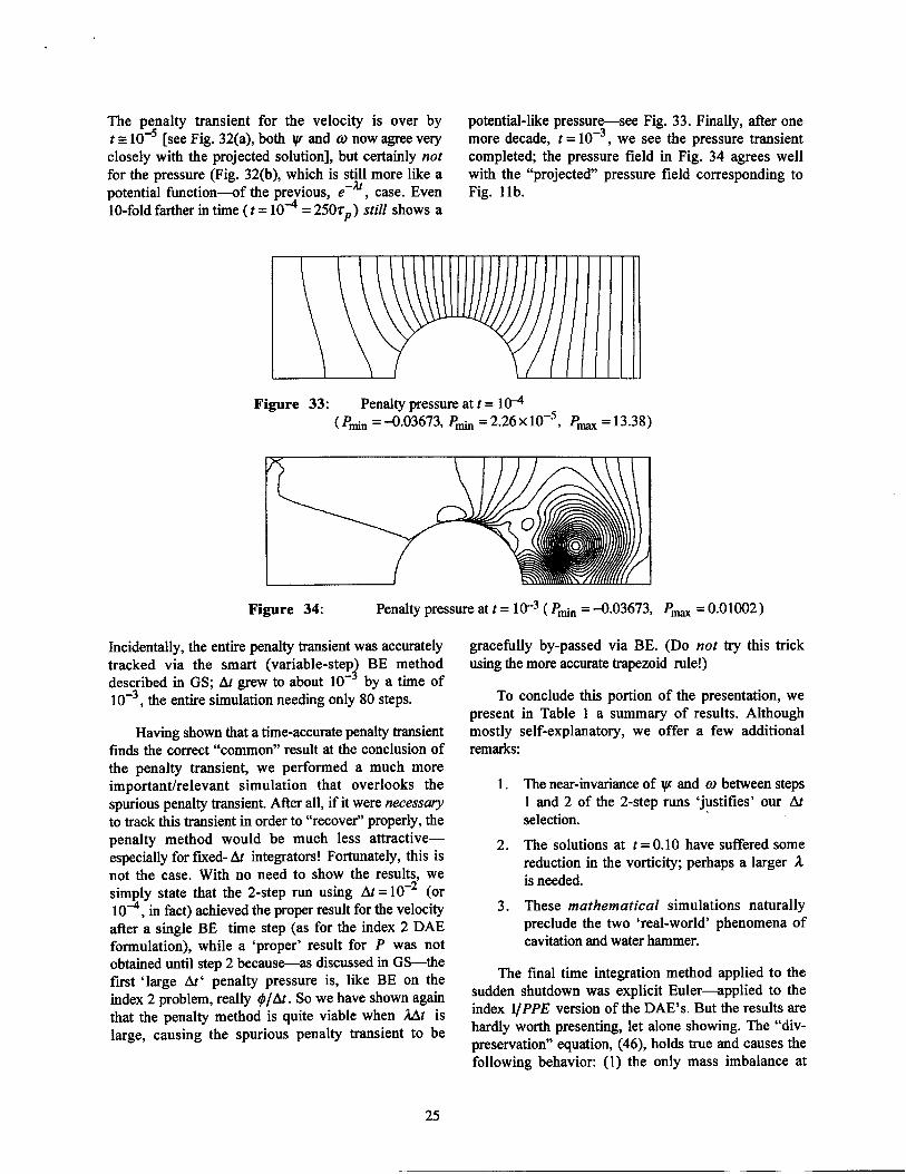
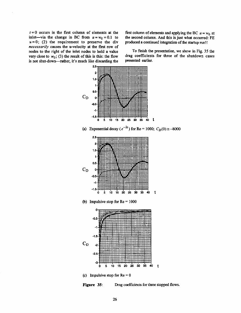
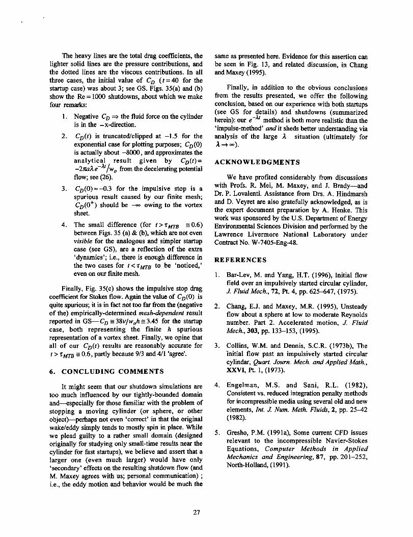
The penalty transient for the velocity is over by potential-like pressur~see Fig. 33. Finally, after onets 10-5 [see Fig. 32(a), both v and @ now agree very more decade, t= 10-3, we see the pressure transientclosely with the projected solution], but certainly not completed; the pressure field in Fig. 34 agrees wellfor the pressure (Fig. 32(b), which is still more like a with the “projected” pressure field corresponding topotential function-of the previous, e-a, case. Even Fig. 1lb.10-fold farther in time (r = 10+ = 250tP) still shows a

Figure 33: Penalty pressure at t= lti( Ptin = -0.03673, Pm = 2.26x 10-5, P- = 13.38)

Figure 34: Penalty pressure at t= 10_3( Ptin = -0.03673, P-= 0.01002)

Incidentally, the entire penalty transient was accuratelytracked via the smart (variable-step BE method

)described in GS; At grew to about 10- by a time of10-3, the entire simulation needing only 80 steps.

Having shown that a time-accurate penalty transientfinds the correct “common” result at the conclusion ofthe penalty transient, we performed a much moreimportant/relevant simulation that overlooks thespurious penalty transient. After all, if it were necessuryto track this transient in order to “recover” properly, thepenalty method would be much less attractive—especially for f~ed- At integrators ! Fortunately, this isnot the case. With no need to show the results, wesimply state that the 2-step run using At= 10-2 (or10A, in fact) achieved the proper result for the velocityafter a single BE time step (as for the index 2 DAEformulation), while a ‘proper’ result for P was not

obtained until step 2 because-as discussed in GS-thefust ‘large At’ penalty pressure is, like BE on theindex 2 problem, really @/At. So we have shown againthat the penalty method is quite viable when 2At islarge, causing the spurious penalty transient to be

gracefully by-passed via BE. (Do not try this trickusing the more accurate trapezoid rule!)

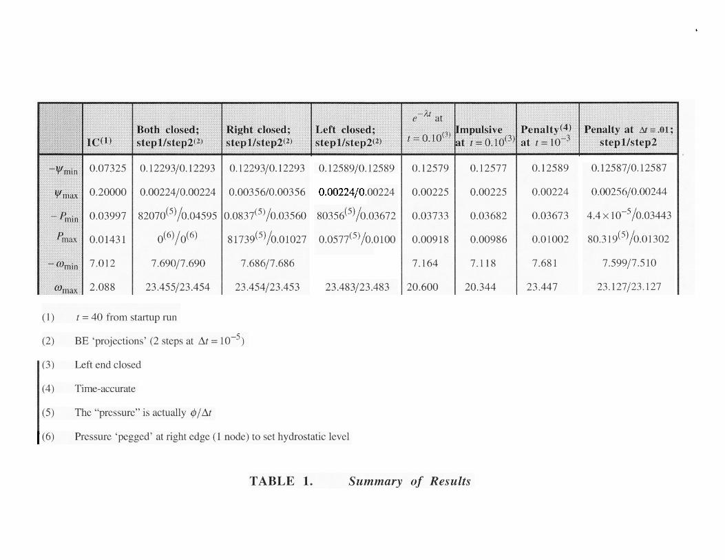
To conclude this portion of the presentation, wepresent in Table 1 a summary of results. Althoughmostly self-explanatory, we offer a few additionalremarks:

1.

2.

3.

The near-invariance of v and co between steps1 and 2 of the 2-step runs ‘justifies’ our Atselection.

The solutions at t=0.10have suffered somereduction in the vorticity; perhaps a larger Ais needed.

These mathematical simulations naturallypreclude the two ‘real-world’ phenomena ofcavitation and water hammer.

The final time integration method applied to thesudden shutdown was explicit Euler—applied to theindex l/PPE version of the DAE’s. But the results arehardly worth presenting, let alone showing. The “div-preservation” equation, (46), holds true and causes thefollowing behavior: (1) the only mass imbalance at

25

t = O occurs in the first column of elements at the fmt column of elements and applying the BC u = WOatinlet—via the change in BC born u = W. = 0.1 to the second column. And this is just what occurred FEu = O; (2) the requirement to preserve the div produced a continued integration of the startup run!!necessarily causes the u-velocity at the first row ofnodes to the right of the inlet nodes to hold a value To finish the presentation, we show in Fig. 35 the

very close to W.; (3) the result of this is this: the flow drag coefficients for three of the shutdown cases

is not shut-down-rather, it’s much like discarding the presented earlier.

0510152025 s0s540 t

(a) Exponential decay (e-h) for Re = 1000; CD(0)s -8000

2.5

2

1.5

1

0.5

0

-0.5

-1

-1.5051015 ti%ti2k40 t

(b) Impulsive stop for Re = 1000

0510152025303540

(c) Impulsivestop for Re = O

t

Figure 35: Drag coefficients for three stopped flows.

26

The heavy lines are the total drag coefllcients, thelighter solid lines are the pressure contributions, andthe dotted lines are the viscous contributions. In allthree cases, the initial value of CD (t= 40 for thestartup case) was about 3; see GS. Figs. 35(a) and (b)show the Re = 1000 shutdowns, about which we makefour remarks:

1. Negative CD - the fluid force on the cylinderis in the - x-direction.

2. CD(t) k truncated/clipped at –1.5 fOr theexponential cue for plotting purposes; CD(O)is actually about -8000, and approximates theanalytical result given by CD(t)=-2nzzAe-z/w0 iiom the decelerating potentialflOW;S= (26).

3. CD(0)= -0.3 for the impulsive stop is aspurious result caused by our finite mesh;CD(O+) should be ~ owing to the vortexsheet.

4. The small difference (for t > ZMTB s 0.6)between Figs. 35 (a)& (b), which are not evenvisible for the analogous and simpler startupcase (see GS), are a reflection of the extra‘dynamics’; i.e., there is enough difference inthe two cases for t< ~~B to be ‘noticed,’even on our finite mesh.

Finally, Fig. 35(c) shows the impulsive stop dragcoefficient for Stokes flow. Again the value of CD(0) isquite spurious; it is in fact not too far from the (negativeof the) empirically-determined mesh-akpendent resultreported in GS- CDs 38v/wOh E 3.45 for the startupcase, both representing the finite h spuriousrepresentation of a vortex sheet. Finally, we opine thatall of our CD(t) results are reasonably accurate fort> ZMTBs 0.6, partly because 9/3 and 4/1 ‘agree’.

6. CONCLUDING COMMENTS

It might seem that our shutdown simulations aretoo much influenced by our tightly-bounded domainand-especially for those familiar with the problem ofstopping a moving cylinder (or sphere, or otherobject)-perhaps not even ‘correct’ in that the originalwake/eddy simply tends to mostly spin in place. Whilewe plead guilty to a rather small domain (designedoriginally for studying only small-time results near thecylinder for fast startups), we believe and assert that alarger one (even much larger) would have only‘secondary’ effects on the resulting shutdown flow (andM. Maxey agrees with us; personal communication) ;i.e., the eddy motion and behavior would be much the

same as presented here. Evidence for this assertion canbe seen in Fig. 13, and related discussion, in Changand Maxey (1995).

Finally, in addition to the obvious conclusionsffom the results presented, we offer the followingconclusion, based on our experience with both startups(see GS for details) and shutdowns (summarizedherein): our e-fi method is both more realistic than the‘impulse-method’ and it sheds better understanding viaanalysis of the large A situation (ultimately forA + m).

ACKNOWLEDGMENTS

We have profited considerably from discussionswith Profs. R. Mei, M. Maxey, and J. Brady-andDr. P. Lovalenti. Assistance from Drs. A. Hindmarshand D. Veyret are also gratefully acknowledged, as isthe expert document preparation by A. Henke. Thiswork was sponsored by the U.S. Department of EnergyEnvironmental Sciences Division and performed by theLawrence Livermore National Laboratory underContract No. W-7405-Eng-48.

REFERENCES

1,

2.

3.

4.

5.

Bar-Lev, M. and Yang, H.T. (1996), Initial flowfield over an impulsively started circular cylinder,J Fluid Mech., 72, Pt. 4, pp. 625-647, (1975).

Chang, E.J. and Maxey, M.R. (1995), Unsteadyflow about a sphere at low to moderate Reynoldsnumber. Part 2. Accelerated motion, J. FluidMech., 303, pp. 133–153, (1995).

Collins, W.M. and Dennis, S.C.R. (1973 b), The‘initial flow past an impulsively started circularcylindar, Quart. Journ. A4ech. and Applied Math.,XXVI, Pt. 1, (1973).

Engelman, M.S. and Sani, R.L. (1982),Consistent vs. reduced integration penalty methodsfor incompressible media using several old and newelements, Int. J Num. A4eth. Fluia%, 2, pp. 25-42(1982).

Gresho, P.M. (1991a), Some current CFD issuesrelevant to the incompressible Navier-StokesEquations, Computer Methods in AppliedMechanics and Engineering, 87, pp. 20 1–252,North-Holland, (1991).

27

6.

7.

8.

9.

Gresho, P.M. (1991b), Incompressible fluiddynamics: Some fundamental formulation issues,Annu. Rev. Fluid A4ech., 23, pp. 413–53, (1991).

Gresho, P.M. and Sani, R.L. (1987), On pressureboundary conditions for the incompressible Navier-Stokes Equations, Znt. J, Num. h4eth. Fluiak, 7,PP. 1111–1145 (1987).

Gresho, P.M. and Sani, R.L. (1997),Incompressible Flow and the Finite ElementMet hod, Vol 1: Advection-Diffus ion andIsothermal Laminar Flow, John Wiley and Sons,Chichester (in Press).

Mei, R. and Lawrence, C.J. (1996), The flow fielddue to a body in impulsive motion, J. FluidMech., 325, pp. 79-111, (1996).

10. Wang, C.-Y. (1968), A note on the drag of animpulsively started circular cylinder, J. Math and ‘Phys., 47, p. 451.

11. Wang, X. and Dalton, C. (1991), Numerical solu-tions for impulsively started and deceleratedviscous flow past a circular cylinder, ht. J. Num.Meth. Fluicik, 12, pp. 383-400 (1991).

28

02c-!m000

Technical Inform

ation Departm

ent • Lawrence Liverm

ore National Laboratory

University of C

alifornia • Livermore, C

alifornia 94551