!!!

!!!

!!!

!!!

!!!

!!!

!!!

!!!

!!!

!!!

!!!

!!!

!!!

!!!

!!!

!!!

!!!

!!!

!!!

!!!

!!!

!!!

!!!

!!!

!!!

!!!

!!!

!!!

!!!

!!!

!!!

!!!

!!!

!!!

!!!

!!!

!!!

!!!

!!!

!!!

!!!

!!!

!!!

!!!

!!!

!!!

!!!

!!!

!!!

!!!

!!!

!!!

!!!

!!!

!!!

!!!

!!!

!!!

!!!

!!!

!!!

!!!

!!!

!!!

!!!

!!!

!!!

!!!

!!!

!!!

!!!

!!!

!!!

!!!

!!!

!!!

!!!

!!!

!!!

!!!

!!!

!!!

!!!

!!!

!!!

!!!

!!!

!!! EidgenossischeTechnische HochschuleZurich

Ecole polytechnique federale de ZurichPolitecnico federale di ZurigoSwiss Federal Institute of Technology Zurich

Homogenization via p-FEM for Problemswith Microstructure

A.M. Matache and C. Schwab

Research Report No. 99-09April 1999

Seminar fur Angewandte MathematikEidgenossische Technische Hochschule

CH-8092 ZurichSwitzerland

Homogenization via p-FEM for Problems with Microstructure

A.M. Matache and C. Schwab

Seminar fur Angewandte MathematikEidgenossische Technische Hochschule

CH-8092 ZurichSwitzerland

Research Report No. 99-09 April 1999

Abstract

A new class of p version FEM for elliptic problems with microstructure isdeveloped. Based on arguments from the theory of n-widths, the existence ofsubspaces with favourable approximation properties for solution sets of PDEsis deduced. The construction of such subspaces is addressed for problemswith (patch-wise) periodic microstructure. Families of adapted spectral shapefunctions are exhibited which give exponential convergence for smooth data,independently of the coe!cient regularity. Some theoretical results on thespectral approach in homogenization are presented. Numerical results showrobust exponential convergence in all cases.

1 Microstructure and n-widths

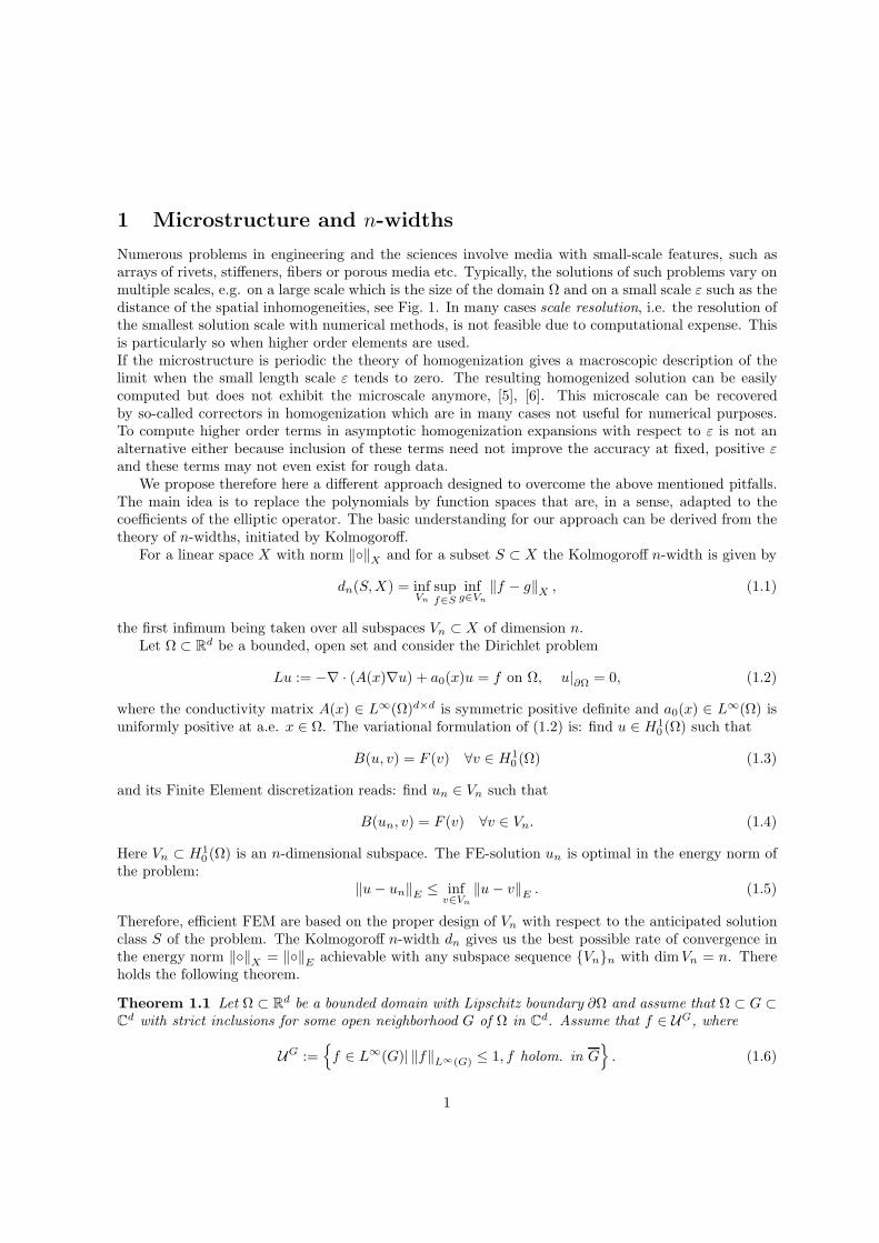
Numerous problems in engineering and the sciences involve media with small-scale features, such asarrays of rivets, sti!eners, fibers or porous media etc. Typically, the solutions of such problems vary onmultiple scales, e.g. on a large scale which is the size of the domain " and on a small scale ! such as thedistance of the spatial inhomogeneities, see Fig. 1. In many cases scale resolution, i.e. the resolution ofthe smallest solution scale with numerical methods, is not feasible due to computational expense. Thisis particularly so when higher order elements are used.If the microstructure is periodic the theory of homogenization gives a macroscopic description of thelimit when the small length scale ! tends to zero. The resulting homogenized solution can be easilycomputed but does not exhibit the microscale anymore, [5], [6]. This microscale can be recoveredby so-called correctors in homogenization which are in many cases not useful for numerical purposes.To compute higher order terms in asymptotic homogenization expansions with respect to ! is not analternative either because inclusion of these terms need not improve the accuracy at fixed, positive !and these terms may not even exist for rough data.

We propose therefore here a di!erent approach designed to overcome the above mentioned pitfalls.The main idea is to replace the polynomials by function spaces that are, in a sense, adapted to thecoe#cients of the elliptic operator. The basic understanding for our approach can be derived from thetheory of n-widths, initiated by Kolmogoro!.

For a linear space X with norm !"!X and for a subset S # X the Kolmogoro! n-width is given by

dn(S,X) = infVn

supf!S

infg!Vn

!f $ g!X , (1.1)

the first infimum being taken over all subspaces Vn # X of dimension n.Let " # Rd be a bounded, open set and consider the Dirichlet problem

Lu := $% · (A(x)%u) + a0(x)u = f on ", u|!! = 0, (1.2)

where the conductivity matrix A(x) & L"(")d#d is symmetric positive definite and a0(x) & L"(") isuniformly positive at a.e. x & ". The variational formulation of (1.2) is: find u & H1

0 (") such that

B(u, v) = F (v) 'v & H10 (") (1.3)

and its Finite Element discretization reads: find un & Vn such that

B(un, v) = F (v) 'v & Vn. (1.4)

Here Vn # H10 (") is an n-dimensional subspace. The FE-solution un is optimal in the energy norm of

the problem:!u$ un!E ( inf

v!Vn

!u$ v!E . (1.5)

Therefore, e#cient FEM are based on the proper design of Vn with respect to the anticipated solutionclass S of the problem. The Kolmogoro! n-width dn gives us the best possible rate of convergence inthe energy norm !"!X = !"!E achievable with any subspace sequence {Vn}n with dimVn = n. Thereholds the following theorem.

Theorem 1.1 Let " # Rd be a bounded domain with Lipschitz boundary "" and assume that " # G #Cd with strict inclusions for some open neighborhood G of " in Cd. Assume that f & UG, where

UG :=!

f & L"(G)| !f!L!(G) ( 1, f holom. in G"

. (1.6)

1

\tex{$\varepsilon$}

Figure 1: Domains with periodic, resp. locally periodic structure.

Assume that A(x) & L"(")d#d and a0(x) & L"(") in (1.2) are positive. Then the solution operatorT : H$1(") ) H1

0 (") to (1.2) is bijective and we define the set S in (1.1) to be

S = T (UG).

Then there holdsC1 exp($r1n

1/d) ( dn(T (UG), E) ( C2 exp($r2n1/d), (1.7)

where Ci and ri > 0 depend only on " and G and on the ellipticity constants of the bilinear form B(·, ·).

For a proof of this theorem, we refer to [9]. From the proof it is clear that results of the type ofTheorem 1.1 hold for practically all well-posed elliptic boundary value problems. We see in particularthat exponential convergence is achievable even if the coe!cients A(x), a0(x) and the boundary "" arevery irregular. The global regularity of the solution in standard Sobolev spaces is very low in thesecases and standard FEM based on piecewise polynomials will only give poor convergence rates.The impact of Theorem 1.1 on numerical computation depends, of course, on whether sequences {Vn}nof subspaces, for which the bounds (1.7) are attained, can be obtained cheaply. Such subspaces arenecessarily problem adapted. Some choices for elliptic problems in two dimensions with stratified quasione-dimensional coe#cients have been proposed in [2]. Here, we present a methodology for determiningsuch subspaces for elliptic problems in divergence form with periodic, oscillating coe#cients. Such

2

homogenization problems have been well investigated by asymptotic analysis (see, e.g. [5, 6] and thereferences there). It turns out, however, that the information on the solution obtained by asymptoticanalysis is insu#cient to construct {Vn}n satisfying (1.7) [7]. For the construction of such {Vn}n, wetherefore present first a more general, non-asymptotic approach to homogenization due to [3].

2 Homogenization

2.1 The homogenization problem

We consider now a particular case of (1.2), namely that the coe#cients A(x) and a0(x) have the specialform A(x/!), a0(x/!), where A(y), a0(y) are 2#- periodic in each variable, i.e.

A(y) = A(y + 2#Zd), a0(y) = a0(y + 2#Zd),

and ! > 0 is small, i.e. we are in the setting of (classical) homogenization. If A is piecewise constant,(1.2) models, for example, the matrix and the fibers of a composite or a bi-material mixture. The righthand side f is assumed to be analytic in " (this is essential for exponential convergence, but spectralconvergence results can be proved if the regularity of f is finite [7], [8]). We denote the solution of (1.2)by u"(x) in order to underline the dependence on !.

We consider (1.2) on the unbounded domain " = Rd and assume that

$*A(x)$ + %|$|2, a0(x) + % > 0, ' $ & Rd at a.e. x & R

d,

with the condition lim|x|%" u"(x) = 0.Next, for & & R and j = 0, 1 we introduce the weighted Sobolev spacesHj

#(Rd), defined as the completion

of C"0 (Rd) with respect to the ! · !j,# norm: Hj

#(Rd) := C"

0 (Rd)&·&j,!

, where for u & C"0 (Rd) we define

!u!2j,# =

#

Rd

$

|k|'j

|Dku(x)|2e2#|x| dx. (2.1)

For a variational formulation of (1.2) on " = Rd, for each ! > 0 we consider the sesquilinear form$(!)[·, ·] : H1

$#(Rd),H1

# (Rd) ) C given by

$(!)[u, v] :=

#

Rd

A%x

!

&

%xu(x) ·%xv(x) + a0%x

!

&

u(x)v(x) dx. (2.2)

It was shown in [3] that there exists &0 > 0, such that for all 0 < & < &0, f &'

H1# (R

d)((

and for all! > 0 there exists a unique weak solution u"(x) & H1

$#(Rd) of the variational problem

$(!)[u", v] =< f, v >(H1! (R

d))"#H1!(R

d), ' v & H1# (R

d). (2.3)

The brackets < ·, · >(H1!(R

d))"#H1!(R

d) on the right hand side in (2.3) stand for the'

H1# (R

d)(( ,H1

# (Rd)

duality paring and are the natural extension of the L2 scalar product in Rd (in the sense that H1# (R

d) #L2(Rd) -= L2(Rd)( #

'

H1# (R

d)((). This means that (1.2) can even be solved when f belongs to a larger

class of functions than L2(Rd), namely to the dual space of H1# (R

d). Such functions are for examplepolynomials or ei<t, ·>, for t & Cd, |Im t| < &. Moreover, the solution operator is continuous from'

H1# (R

d)((

into H1$#(R

d).

3

Consider now the parameter dependent family of bounded linear functionals on H1# (R

n) given bythe standard Fourier waves ei<t, ·> &

'

H1# (R

d)((

parametrized with respect to t & Rd. Then, for eachfrequency t & Rd we denote by '(x/!, !, t) & H1

$#(Rd) the unique weak solution of (2.3) with respect

to f(·) = ei<t, ·>. It has been shown in [3] that '(y, !, t) = ((y, !, t)ei"<t, y>, with ((y, !, t) & H1per(Q)

being the solution of the so-called unit cell problem in Q := ($#,#)d: For ! > 0 and t & Cd, find((y, !, t) & H1

per(Q) such that

%(!, t)[(, v] = !2(1, v)0, Q, ' v & H1per(Q). (2.4)

The bilinear form %(!, t)[·, ·] : H1per(Q),H1

per(Q) ) C in (2.4) is defined by

%(!, t)[(, v] =

#

Q

A(y)%y

'

((y)ei"<t, y>(

·%y (v(y)ei"<t, y>) + !2a0(y)((y)v(y) dy.

The significance of the unit-cell problem (2.4) lies in the fact that for every f & L2(Rd), the solutionu"(x) of (2.3) has a representation as a (generalized) Fourier-Inversion integral

u"(x) =1

(2#)d/2

(B)#

Rd

f(t)ei<t, x>(%x

!, !, t

&

dt, (2.5)

with integral kernel '(x/!, !, t) = ((x/!, !, t)ei<t, x>. The integral in (2.5) has to be understood in thesense of Bochner integral of Banach space valued function (see [3] for a definition). Henceforth, we

write) (B)

for such integrals. The representation (2.5) will be the basis for our construction of {Vn}n.We have, see ([7], [8])

Proposition 2.1 There exists ) > 0 depending only on A, a0, &, such that for any

t & D$ :=*

t & Cd : |Im t| < )

+

and every ! > 0, problem (2.4) admits a unique solution ((·, !, t) & H1per(Q). Moreover,

a) for any fixed ! > 0, the kernel ((·, !, t) is an analytic H1per(Q)-valued function of t in the strip

D$ # Cd,b) for any (!, t) in Rd+1, ((·, !, t) is real analytic at (!, t) (with domain of analyticity depending on

(!, t), however).

Remark 2.2 A very useful regularity property holds for the kernel '(·/!, !, t). It has been shown in [8]that '(·/!, !, t) can be extended as analytic and uniformly bounded function of t in the strip D$ withvalues in H1

$#(Rd), i.e. '(·/!, !, t) & A

'

D$, H1$#(R

d)(

. L"'

D$, H1$#(R

d)(

, with bounds independentof ! > 0.

2.2 Approximation on Rd

We return to the question raised in Section 1, i.e. if subspace sequences {Vn}n (possibly dependingon !) can be found which realize the convergence rates (1.7). One approach would be to incorporateanalytic results from classical homogenization, i.e. an asymptotic expansion of u"(x) as ! ) 0 ([5], [6]),into the FEM. This ”classical homogenization approach” can also be derived from (2.5) (see [3], [8]),but does not give subspaces Vn which achieve (1.7) [7]. To do so, we must exploit the analytic structure

4

of the data f and of the kernel '(x/!, !, t) in (2.5) indicated in Remark 2.2.The idea is to approximate the Fourier-Bochner integral (2.5) by a finite sum, which is obtained bytruncating a (generalized) Poisson summation formula.For N & N and h > 0 define the trapezoidal approximation of (2.5)

u"N,h(x) = 1[$"

h ,"h ]d(x)

1

(2#)d/2hd

$

k!Zd(N)

f(kh)(%x

!, !, kh

&

ei<kh, x>, (2.6)

whereZd(N) =

*

k & Zd : |kj | ( N, ' j = 1, . . . , d

+

.

Definition 2.3 We say a function f fulfills the ’usual assumptions’ if f & L2(Rd), and its Fouriertransformation f(·) can be extended to a holomorphic function in the strip D$, with ) as in Proposi-tion 2.1, which satisfies the following growth condition:

|f(z)| ( Cf e$%|z|, ' z & D$, (2.7)

for some positive constants Cf ,* > 0.

Our main result on the trapezoidal approximation (2.6) of the Fourier-Bochner integral (2.5) is (see [8]for a proof) :

Proposition 2.4 Let us assume that f satisfies the ’usual assumptions’ as in Definition 2.3, L > 0 isarbitrary and the step size h is given by

h =

,

#)

*N

-1/2

, N + 4)L2

*#. (2.8)

Then the error )N (f, h)(·) := u"(·)$ u"N,h(·), with u"

N,h(·) as in (2.6), decays exponentially with respectto N in the ! · !0,$2# , ! · !H1

#2!(($L,L)d)-norms:

!)N(f, h)(·)!0,$2# + !)N(f, h)(·)!H1#2! (($L,L)d) ( C0Cf

1

*de$(&%$N/d)1/2, (2.9)

with the constant C0 = C(%, &, d,*) independent of !, N and L.

Remark 2.5 Let VN" := Span

!

Re''

·" , !, kh

(

, Im''

·" , !, kh

(

: k & Zd(N)

"

. Then n = dimVN" =

O(Nd), and we see from (2.9) that u" is approximated by VN" at a robust (in !) exponential rate, but

comparing with (1.7) the approximation is not optimal in the sense of n -width.

2.3 Periodic setting

We will now exhibit an example of subspaces where the optimal bound (1.7) can be achieved. In order topresent the ideas clearly, we consider the bounded domain in the periodic setting (non-periodic below).Let 1/! & N and " = (0, 2#)d be an 1/! fold repetition of the scaled unit cell Q = !Q:

" =.

k!Zd : 0'ki<1/"

!%

(2k + 1)# + Q&

.

5

Likewise A(y) = A(y+2k#), a0(y) = a0(y+2k#), ' k & Zd and assume that f(x) = f(x+2k#) & L2(").Denote by u" the solution of the following problem

u" & H1per(") : L"u" = f in ", (2.10)

where L" is the second order, strongly elliptic operator

L"u = $% ·%

A%x

!

&

%u&

+ a0%x

!

&

u.

Discrete analog of (2.5). Let us denote by f' the Fourier coe#cients of f with respect to the basis{ei<', x>}'!Zd # L2(") :

f(x) =$

'!Zd

f'ei<', x>. (2.11)

Then, it can be easily seen that

u"(x) =$

'!Zd

f'(%x

!, !, +

&

ei<', x> =$

'!Zd

f''%x

!, !, +

&

, (2.12)

where ((·, !, t) is as in (2.4) and the series (2.12) converges in the Banach space H1per(").

Define for µ & N and ! > 0

Vµ" := Span

!

Re'% ·!, !, +

&

, Im'% ·!, !, +

&

, + & Zd, 0 ( |+ | ( µ

"

. (2.13)

Then n = dim (Vµ" ) = O(µd) and the following approximation result holds

Proposition 2.6 Assume that f & Aper("). Then, for every ! > 0 such that 1/! & N,

infv!Vµ

#

!u" $ v!1,! ( Ce$bµ = Cexp($bn1/d), (2.14)

where C, b > 0 are independent of !, µ, depend only on f .

We see that the subspace sequence {Vn}n given by!

Vµ"

"

µin (2.13) (with n = O(µd)) realizes the

optimal rate in Theorem 1.1.

3 Generalized p-FEM in homogenization

So far, Propositions 2.4, 2.6 indicated that for the model problem

L"u" := $% ·%

A%x

!

&

%u"(x)&

+ a0%x

!

&

u"(x) = f(x) (3.1)

in either the unbounded domain or the periodic setting, with analytic f , the solution u" can be approx-imated very well by linear combinations of the kernel '(x/!, !, t) (resp. ((x/!, !, t)ei<t, x>).In a general, bounded domain " # Rd we propose to construct therefore generalized FE-spacesSp, µ(", T ) which consist of the “usual” piecewise polynomial functions of degree p which are aug-mented by special, so-called ‘micro’ shape functions of ’degree’ µ derived from the sampled kernel (.Clearly, these shape functions are generally not explicitly known and must be computed numericallyby a FE-solution of the unit-cell problem.

6

\tex{$2\pi\varepsilon$}

\tex{$\hat Q$}

\tex{$Q = \varepsilon \hat Q$}

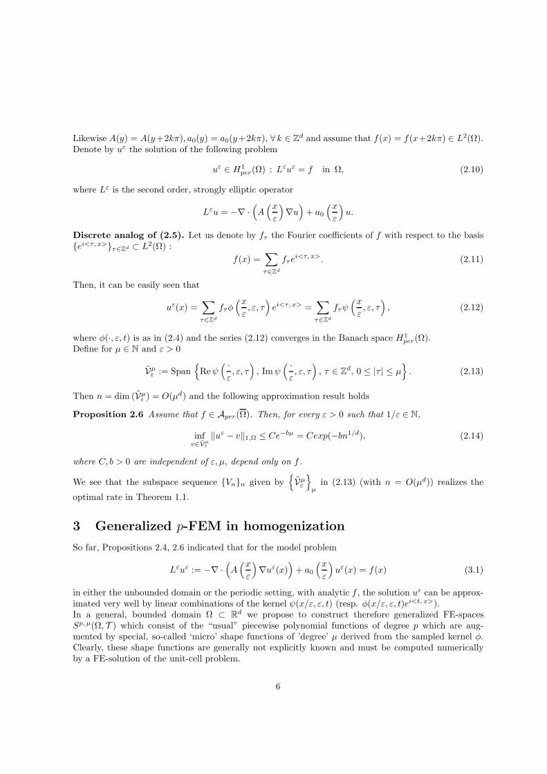
Figure 2: Geometric mesh T for unit cell Q with crack.

3.1 Computation of microscale shape functions.

Let ! > 0, t & Cd be given, and T an a#ne mesh on the unit cell Q. Then the FE formulation for theunit cell-problem (2.4) reads: Find (hp(·, !, t) & Sp, 1

per (Q, T ), such that

%(!, t)[(hp, v] = !2(1, v)0, Q, ' v & Sp, 1per (Q, T ), (3.2)

where the FE space Sp, 1per (Q, T ) is defined by

Sp, 1per (Q, T ) :=

/

u & H1per(Q) : u

0

0

0

0

K

& S p(K), 'K & T1

(3.3)

and S p(K) is the space of polynomials of degree at most p on K. The design of T , p must takeinto account regularity of the solution, e.g. if the unit cell problem has a crack, then the solution((y, !, t) & B2

((Q), the countably normed space [1], and hp-FEM with a geometrical mesh refinementtowards the crack-tips must be employed for the solution of the unit-cell problem. (see Fig. 2).

The kernel ((·/!, !, t) can be directly employed for computational purposes, and we see from (2.9),(2.14) that collocation of ((·/!, !, t) at various sets of collocation points N = {tj} gives systems of shapefunctions with very good approximation properties for elliptic problems with periodic microstructure.

Since ((y, !, t) is analytic in t (Proposition 2.1), choosing the collocation points N = {kh, k & Zd(N)}

with h ) 0 as in (2.8) will lead to almost linear dependence of (hp(y, !, tj), tj & N ; these functions aretherefore unsuitable as basis for p-FEM in numerical computations. We propose here a methodologyto derive a well conditioned set of micro shape functions from the collocated kernels '(·/!, !, tj), whichis based on ’oversampling + SVD’. As a byproduct, this approach will also reduce the number of microshape functions substantially. To this end, we select the collocation points

N := {tj : j = 1, . . . , µ} , µ > µ (3.4)

and orthogonalize by SVD the matrix of coe#cient vectors of the FE approximations to the ((y, !, tj), tj &N . Select thereforeN(y) to be a well conditioned basis of Sp, 1

per (Q, T ) and denote by %j(!) the coe#cient

vector of (hp(y, !, tj) with respect to N(y), i.e. (hp(y, !, tj) = %j(!))N(y). Compute the SVD of thematrix of coe#cient vectors %j(!), j = 1, . . . , µ

[%1(!), . . . ,%µ(!)] = Udiag(,1, . . . ,,µ)V)

7

and define the basis functions

(j

%x

!, !&

:= U)j N

%x

!

&

, j = 1, . . . , µ, (3.5)

with U j being the j-th column of U .

Note that Span!

(j(y, !) : j = 1, . . . , µ"

= Span {(hp(y, !, tj) : tj & N}. Define further the microspace

Mµ" = Span

!

(j

%x

!, !&

: j = 1, . . . , µ+ 1"

, (3.6)

where µ = 0, . . . , µ(, µ( = inf{j : ,j > tol} and tol is a parameter of order of machine precision.

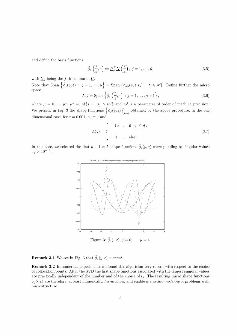
We present in Fig. 3 the shape functions!

(j(y, !)"µ

j=0obtained by the above procedure, in the one

dimensional case, for ! = 0.001, a0 / 1 and

A(y) =

2

3

4

3

5

10 , if |y| ( &2 ,

1 , else .

(3.7)

In this case, we selected the first µ + 1 = 5 shape functions (j(y, !) corresponding to singular values,j > 10$10.

!4 !3 !2 !1 0 1 2 3 4!0.2

!0.15

!0.1

!0.05

0

0.05

0.1

0.15

0.2

! = 0.001: µ = 4; 5 linear independent shape functions (orthogonalized by SVD)

Figure 3: (j(·, !), j = 0, . . . , µ = 4.

Remark 3.1 We see in Fig. 3 that (1(y, !) / const.

Remark 3.2 In numerical experiments we found this algorithm very robust with respect to the choiceof collocation points. After the SVD the first shape functions associated with the largest singular valuesare practically independent of the number and of the choice of tj . The resulting micro shape functions(j(·, !) are therefore, at least numerically, hierarchical, and enable hierarchic modeling of problems withmicrostructure.

8

3.2 Construction of generalized FE spaces.

Let " # Rd be an open, bounded polygonal domain and assume that f & L2("). We denote by u" theunique weak solution of the following boundary value problem: find u" & H1

0 ("), such that

#

!

A%x

!

&

%u" ·%v + a0%x

!

&

u"v dx = (f, v)0,!, ' v & H10 ("). (3.8)

It is well known [5], [6] that in homogenization on bounded domains there arise boundary correctorsthat are not accounted for in (2.5). In the design of Sp, µ(", T ) we need to account for them. We dealwith this by selecting the (macro) mesh T of the generalized FEM properly. To motivate this selection,let

Vµ" := Span

/

ReD%t '

% ·!, !, 0

&

, * & Nd, |*| = 2k, |*| ( µ,

ImD%t '

% ·!, !, 0

&

, |*| = 2k + 1, |*| ( µ

1

, (3.9)

Vµ" := Span

/

Re v"%, * & Nd, |*| = 2k, |*| ( µ, (3.10)

Im v"%, |*| = 2k + 1, |*| ( µ

1

,

where by D%t we denote the partial derivative of order * with respect to t : D%

t := "%1t1 "%2

t2 . . . "%dtd ,

|*| = *1 + . . . + *d and v"% & H1(") is the solution of the following boundary value problem withhomogeneous right hand side and inhomogeneous boundary data :

$% ·%

A%x

!

&

%v"%

&

+ a0%x

!

&

v"% = 0 in ",

v"%

0

0

0

0

!!

= $D%t '

% ·!, !, 0

&

0

0

0

0

!!

, * & Nd. (3.11)

SetVµ" =

%

Vµ" + Vµ

"

&

6

H10 ("). (3.12)

Then the following result holds [8, 7] :

Proposition 3.3 Assume that f & A(") and let u" be the solution of (3.8). Then, there exist positiveconstants depending on f , but independent of ! and µ, such that

infv!Vµ

#

!u" $ v!1,! ( Ce$bµ. (3.13)

This indicates that '(·/!, !, t) for small t are most important for problems with smooth data f , sinceD%

t '(·/!, !, 0) solves (2.2) with f = (ix)%; the space Vµ" is needed here to enforce the boundary con-

ditions. We observe that Vµ" is spanned by products of ’micro’ shape functions D%

t ((·/!, !, 0) timespolynomials of degree at most µ. The correctors v"% in (3.11) are solutions of the homogeneous equationL"u" = 0 in " with inhomogeneous boundary data [5, 6]. The spaces Sp 0Mµ

" approximate solutionsof L"u" = 0 locally at a spectral rate (see [7] or [8] Proposition 3.12).Of course, in the O(!) vicinity of "", the structure of the solution is not anymore well described by therepresentation (2.5); hence there the subspaces Mµ

" in (3.6) are expected to have poor approximation

9

\tex{$u=0$}\tex{$n^\top A \nabla u=0$}

\tex{$u=0$} \tex{$u=0$}

\tex{$n^\top A \nabla u=0$}\tex{$u=0$}

\tex{$u=0$}

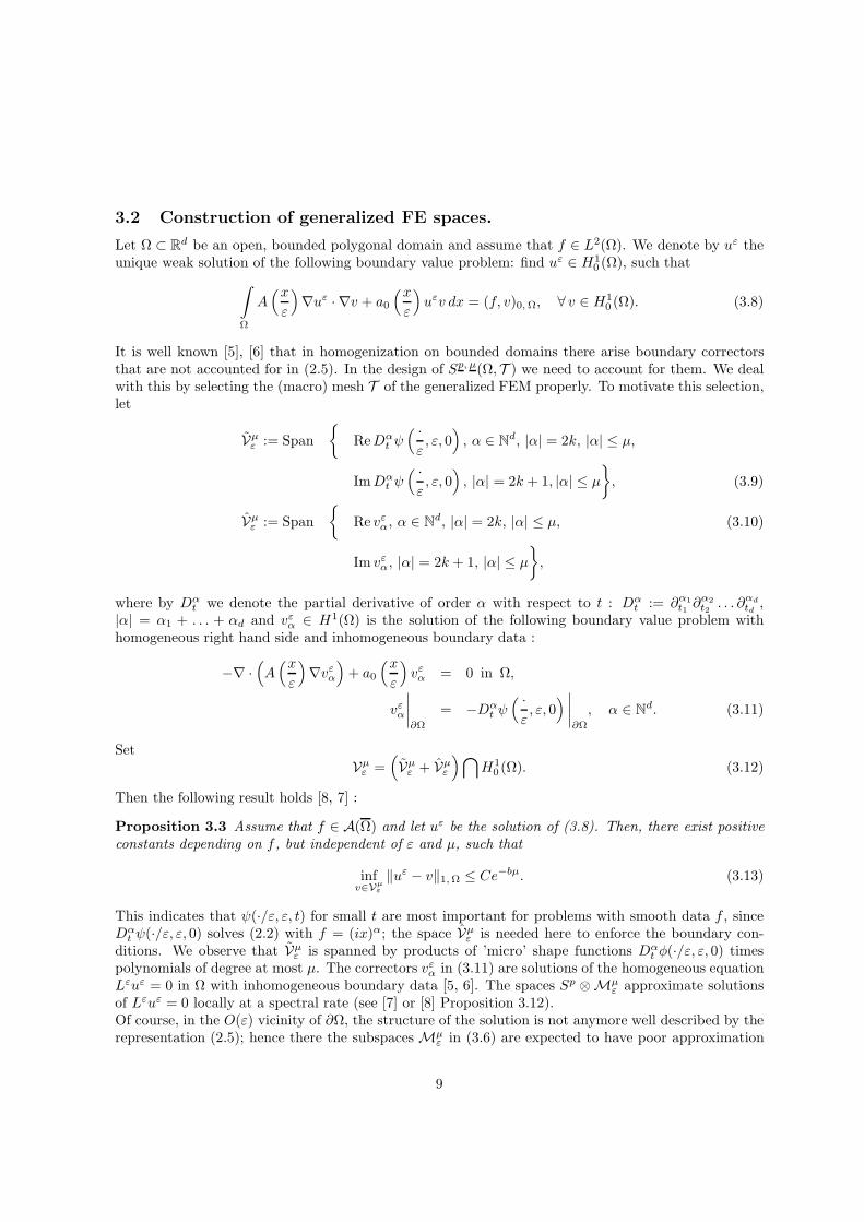
Figure 4: Macro mesh T (bold lines) for cracked panel with crack in each micro-cell (thin lines).Geometric mesh refinement towards ’macro’ singularity at •.

properties. Accordingly, we compose the finite element mesh T = Tint 1 Tb 1 Tsing of three parts : aquasiuniform ’interior’ part (Tint) and a refined ’boundary’ part consisting of elements abutting at acorner or at a singularity (Tsing) or elongated elements abutting at the boundary (Tb), see Fig. 4 for anexample. Note that in Tint the element size is independent of !.Denote by p = {pK}K!T a degree vector and define the finite element space

Sp(", T ) =

/

u & H1(") : u

0

0

0

0

K

& SpK (K), 'K & T1

,

where SpK (K) is elemental polynomial space. Define the micro degree vector µ = {µK}K!T . Then letus introduce the generalized FE-space

Sp, µ(", T ) =

/

u & H1(") : u

0

0

0

0

K

& SpK (K)0MµK" , 'K & T

1

(3.14)

10

and set Sp, µ0 (", T ) = Sp, µ(", T ) .H1

0 (").Strictly speaking, Sp, µ(", T ) also depends on T , p used in (3.3) and on the set N of collocation points.However, if T is su#ciently fine and p in (3.3) su#ciently large, the (hp will converge quasioptimallyand Mµ

" will practically not depend on T , p. We therefore omit T , p in (3.14). Likewise, the collocationset N is not important (see Remark 3.2) and is also omitted. The vector p = {pK}K!T we call the’macro’ polynomial degree, whereas µ = {µK}K!T is called the ’micro’ degree of the generalized p-FEM.Therefore, the generalized FE space Sp, µ(", T ) in (3.14) accounts for both scales, ’micro’ and ’macro’.The ’micro’ degree vector µ is variable; in elements near corner singularities we omit generalized shapefunctions :

2

3

4

3

5

µK-= pK , if K & Tint 1 Tb,

0 , if K & Tsing.

Note that in the elongated elements near the boundary, but not abutting corners, also µK-= pK . This

is necessary to resolve the tangential fine structure of u". Note further that since M0" = Span {1} if

a0 / const (see Remark 3.1), we get that

Sp(", T ) # Sp, µ(", T ), (3.15)

i.e. we have a generalized p-FEM. Moreover, (3.15) ensures that the spaces Sp, µ(", T ) are dense inL2("), as pK ) 2. The generalized FE formulation finally reads: find u"

FE & Sp, µ0 (", T ), such that

#

!

A%x

!

&

%u" ·%v + a0%x

!

&

u"v dx = (f, v)0,!, ' v & Sp, µ0 (", T ). (3.16)

4 Numerical Results.

4.1 Set up and basic results

We present here preliminary numerical results obtained with the generalized FEM. The goal of theexperiments is to validate our approach and to get insight on the practical selection of pK and µK ,as well as on the mesh design. We restrict our numerical examples to problem (3.8) in one dimensionand show the performance of the generalized p-FEM with A(·) as in (3.7) and a0 / 0, on a fixed meshT = Tint 1 Tb with Tb covering 4 periods of length 2#! at each boundary point and only one elementK & Tint. Note that in one dimension Tsing = 3. As right hand side we choose f(x) = exp(x); the exactsolution is in this case piecewise analytic, but non-polynomial on the microscale.

As ’micro’ shape functions we employ!

(µ(y, !)"

µobtained as in (3.4)–(3.7) by solving the unit cell

problem (2.4) with a0 / 1, however. In agreement with Proposition 2.4 we choose the set of collocationpoints N = {tj(µ) = j/

4µ : j = 1, . . . , µ} corresponding to µ = 64.

Note that computation of the sti!ness matrix in (3.16) needs only a fixed number of operations, indepen-dent of !. This is due to the periodicity of the coe#cients A(·), a0(·) and of the ’micro’ shape functions(µ(·, !). In fact, integrals of products of micro shape functions (µ(y, !)(µ$(y, !) times monomials up todegree 2pK over the unit cell Q have to be computed only once.

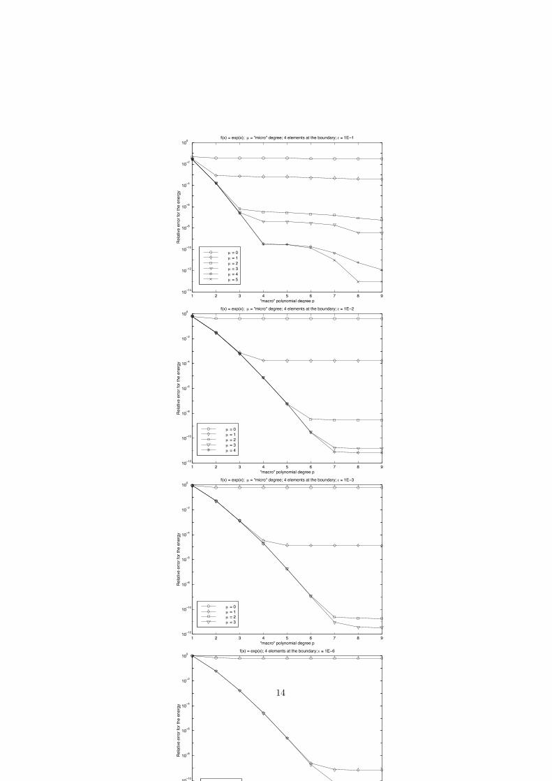
The goal of the numerical experiments is to show robust (with respect to !) exponential convergence.In Fig. 5 we present the relative error of the energy versus ’macro’ polynomial degree pK = p, 'K & T ,by increasing ’micro’ degree µ := µK , K & Tint, and for di!erent ! scales varying from -= 10$6 upto -= 10$1. We see that taking µ = 0, which corresponds to the case when only macroscopic shape

11

functions are used, we do not achieve convergence (only in the case ! -= 10$1 a very slow convergencehardly visible in Figure 5 occurs, since here the scales are resolved, however the low solution regularitystalls the spectral convergence). For µ > 0 and increasing p we get exponential convergence, however asaturation occurs at levels depending only on µ. To achieve robust exponential convergence one has toaugment simultaneously the standard polynomial spaces and the number of microscale shape functions.

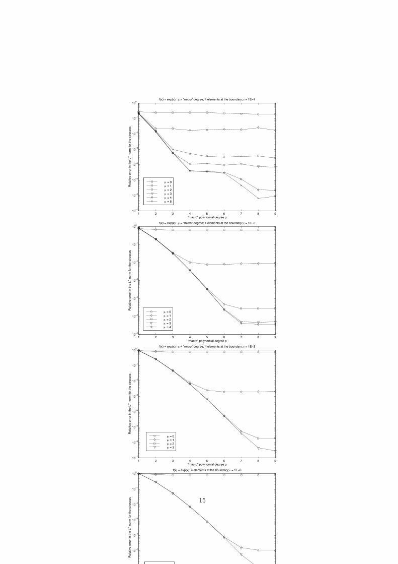
Fig. 6 shows exponential convergence with respect to the (stronger) W 1,"(") - norm, namely thatthe convergence rate for the stresses

7

7

7

7

A%x

!

& d

dx(u" $ u"

FE)

7

7

7

7

L!($1,1)

is also exponential and independent of !.

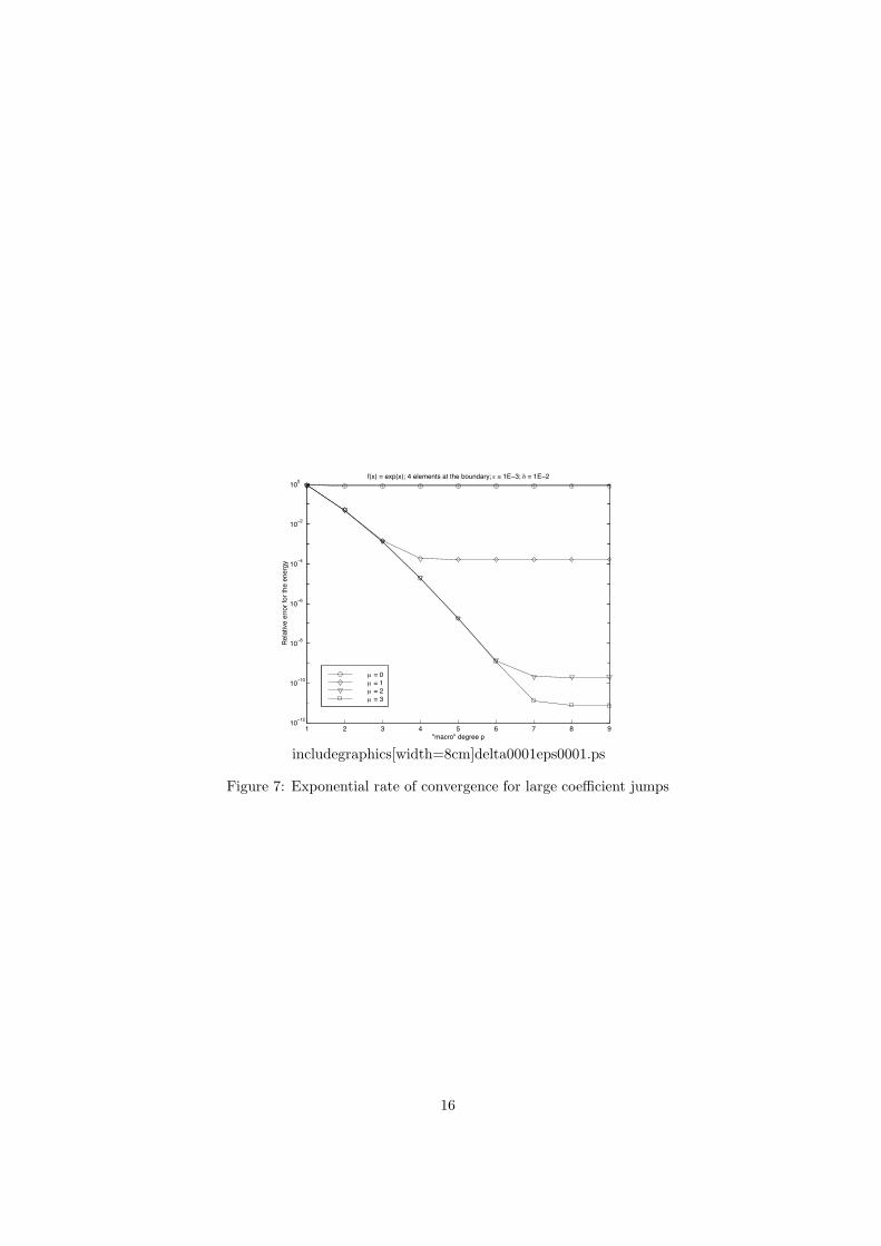
4.2 Jumps in coe!cients

Next, we consider the performance of our approach if the coe#cient A(·) has a very large jump )$1 =Amax/Amin, where Amax := maxy!Q A(y) and Amin := miny!Q A(y)

A(y) =

2

3

4

3

5

)$1 , if |y| ( &2 ,

1 , else .

(4.1)

As ) ) 0, we found the generalized p-FEM to be stable. Comparing Fig. 7 and Fig. 5 (for ) = 0.1)we see that the convergence is insensitive to decreasing ), the error decay is practically the same for) = 0.1, 0.01, 0.001, but at fixed µ the error saturation occurs somewhat earlier as ) ) 0.

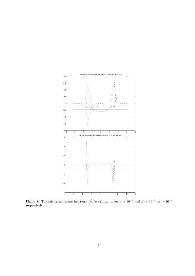
4.3 Singular perturbation and homogenization

Finally, we investigate the performance of our approach if the di!erential operator L" = L"( in (3.1)

is singularly perturbed, in the sense that the principal part depends additionally on another smallparameter 0 < - << 1 in the following way

L"(u

"( = $-2% ·

%

A%x

!

&

%u"((x)

&

+ a0%x

!

&

u"((x). (4.2)

We have a problem with multiple scales : in the vicinity of each discontinuity of A(x/!), a boundarylayer of thickness - appears for - < !. A conventional FEM would thus be required to resolve thesmallest scale -. In our approach, the singular perturbation is taken care of by the unit-cell problem(2.4), which is, for -/! << 1, itself singularly perturbed. Fig. 8 shows the {(µ(y, !)}µ=0,...,3 for (4.2)and for a0 / 1, A(·) as in (3.7). The layers of thickness O(-/!) are clearly visible.

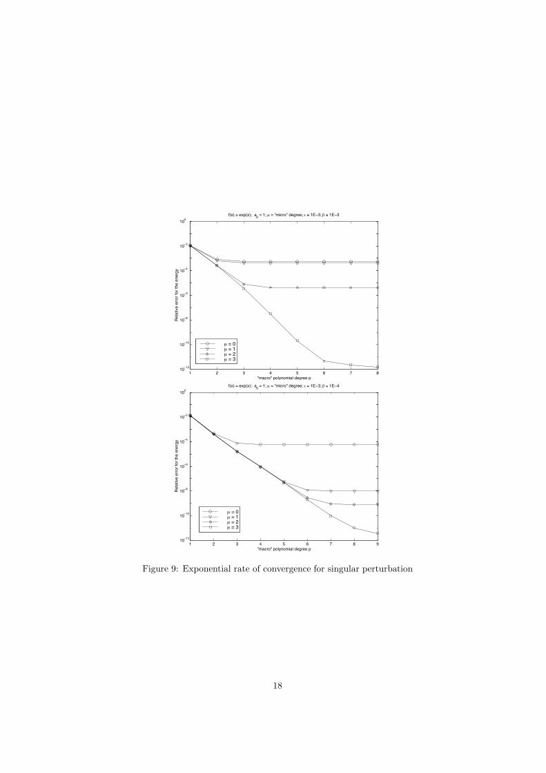
The exponential error decay with respect to the ’macro’ (pK = p, 'K & T ), respectively ’micro’(µK = µ for K & Tint) degree is shown in Fig. 9 for ! -= 10$3 and - -= 10$3, - -= 10$4, respectively. Asbefore, in elements near the boundary (K & Tb) we omit the microscale shape functions (i.e. µK = 0),while in the interior element K & Tint we choose µK = 0, . . . , 3.

Our experiments show clearly that the generalized p-FEM performs equally well for - = 1 and- = 10$3, 10$4, over a wide range of !, from -/! >> 1 to -/! << 1. We emphasize that asymptoticexpansions for the limiting cases -/! ) 0 or !/- ) 0 di!er substantially, as do the limits. Thegeneralized FEM performs robustly over the whole range of -/!.

12

References

[1] I. Babuska, B. Q. Guo, Regularity of the solution of elliptic problems with piecewise analyticdata. Part 1: Boundary value problems for linear elliptic equation of second order, SIAM J.Math. Anal., 19 (1988), pp. 172-203.

[2] I. Babuska, G. Caloz, J. Osborn, Special finite element methods for a class of second order ellipticproblems with rough coe#cients, SIAM J. Numer. Anal., 31 No. 4, (1994), pp. 945-981.

[3] R. C. Morgan, I. Babuska, An approach for constructing families of homogenized equations forperiodic media. I: An integral representation and its consequences, SIAM J. Math. Anal. Vol. 22,No. 1 (1991) pp. 1-15. II: Properties of the kernel, SIAM J. Math. Anal. Vol. 22, No. 1 (1991)pp. 16-33.

[4] T. Hou, X.-H. Wu, Z. Cai, Convergence of a multiscale finite element method for elliptic problemswith rapidly oscillating coe#cients, (to appear in Math. Comp.).

[5] O. A. Oleinik, A. S. Shamaev, G. A. Yosifian, Mathematical Problems in Elasticity and Homoge-nization, North-Holland (1992).

[6] A. Bensoussan, J.L. Lions and G. Papanicolau, Asymptotic Analysis for Periodic Structures,North Holland, Amsterdam (1978).

[7] A.M. Matache, Spectral and p-Finite Elements for homogenization problems, Doctoral Disserta-tion (in preparation).

[8] A.M. Matache, I. Babuska and C. Schwab, Generalized p-FEM in homogenization, Report 99-01,Seminar for Applied Mathematics, ETH Zurich, Switzerland.

[9] J.M. Melenk, On n-widths for elliptic problems, Report 98-02, Seminar for Applied Mathematics,ETH Zurich, Switzerland (in press in J. Math. Anal. Appl.).

13

1 2 3 4 5 6 7 8 910

!14

10!12

10!10

10!8

10!6

10!4

10!2

100

Re

lative

err

or

for

the

en

erg

y

"macro" polynomial degree p

f(x) = exp(x); µ = "micro" degree; 4 elements at the boundary; ! " 1E!1

µ = 0

µ = 1

µ = 2

µ = 3

µ = 4

µ = 5

1 2 3 4 5 6 7 8 910

!12

10!10

10!8

10!6

10!4

10!2

100

Re

lative

err

or

for

the

en

erg

y

"macro" polynomial degree p

f(x) = exp(x); µ = "micro" degree; 4 elements at the boundary; ! " 1E!2

µ = 0

µ = 1

µ = 2

µ = 3

µ = 4

1 2 3 4 5 6 7 8 910

!12

10!10

10!8

10!6

10!4

10!2

100

Re

lative

err

or

for

the

en

erg

y

"macro" polynomial degree p

f(x) = exp(x); µ = "micro" degree; 4 elements at the boundary; ! " 1E!3

µ = 0

µ = 1

µ = 2

µ = 3

10!10

10!8

10!6

10!4

10!2

100

Re

lative

err

or

for

the

en

erg

y

f(x) = exp(x); 4 elements at the boundary; ! " 1E!6

14

1 2 3 4 5 6 7 8 910

!7

10!6

10!5

10!4

10!3

10!2

10!1

100

Re

lative

err

or

in t

he

L#

no

rm f

or

the

str

esse

s

"macro" polynomial degree p

f(x) = exp(x); µ = "micro" degree; 4 elements at the boundary; ! " 1E!1

µ = 0

µ = 1

µ = 2

µ = 3

µ = 4

µ = 5

1 2 3 4 5 6 7 8 910

!6

10!5

10!4

10!3

10!2

10!1

100

Re

lative

err

or

in t

he

L#

no

rm f

or

the

str

esse

s

"macro" polynomial degree p

f(x) = exp(x); µ = "micro" degree; 4 elements at the boundary; ! " 1E!2

µ = 0

µ = 1

µ = 2

µ = 3

µ = 4

1 2 3 4 5 6 7 8 910

!7

10!6

10!5

10!4

10!3

10!2

10!1

100

Re

lative

err

or

in t

he

L#

no

rm f

or

the

str

esse

s

"macro" polynomial degree p

f(x) = exp(x); µ = "micro" degree; 4 elements at the boundary; ! " 1E!3

µ = 0

µ = 1

µ = 2

µ = 3

!6

10!5

10!4

10!3

10!2

10!1

100

Re

lative

err

or

in t

he

L#

no

rm f

or

the

str

esse

s

f(x) = exp(x); 4 elements at the boundary; ! " 1E!6

µ = 0

15

1 2 3 4 5 6 7 8 910

!12

10!10

10!8

10!6

10!4

10!2

100

Re

lative

err

or

for

the

en

erg

y

"macro" degree p

f(x) = exp(x); 4 elements at the boundary; ! " 1E!3; $ = 1E!2

µ = 0

µ = 1

µ = 2

µ = 3

includegraphics[width=8cm]delta0001eps0001.ps

Figure 7: Exponential rate of convergence for large coe#cient jumps

16

!4 !3 !2 !1 0 1 2 3 4!0.4

!0.3

!0.2

!0.1

0

0.1

0.2

0.3

0.4

The first microscale shape functions for ! " 1E!3 and % " 1E!4

!4 !3 !2 !1 0 1 2 3 4!6

!4

!2

0

2

4

6

The first microscale shape functions for ! " 1E!3 and % " 1E!5

Figure 8: The microscale shape functions {(µ(y, !)}µ=0,...,3 for ! 5 10$3 and - 5 10$4, - 5 10$5

respectively

17

1 2 3 4 5 6 7 810

!12

10!10

10!8

10!6

10!4

10!2

100

Re

lative

err

or

for

the

en

erg

y

"macro" polynomial degree p

f(x) & exp(x); a0 = 1; µ = "micro" degree; ! " 1E!3; % " 1E!3

µ = 0µ = 1µ = 2µ = 3

1 2 3 4 5 6 7 8 910

!12

10!10

10!8

10!6

10!4

10!2

100

Re

lative

err

or

for

the

en

erg

y

"macro" polynomial degree p

f(x) & exp(x); a0 = 1; µ = "micro" degree; ! " 1E!3; % " 1E!4

µ = 0µ = 1µ = 2µ = 3

Figure 9: Exponential rate of convergence for singular perturbation

18

Research Reports

No. Authors Title

99-09 A.M. Matache, C. Schwab Homogenization via p-FEM for Problemswith Microstructure

99-08 D. Braess, C. Schwab Approximation on Simplices with respect toWeighted Sobolev Norms

99-07 M. Feistauer, C. Schwab Coupled Problems for Viscous IncompressibleFlow in Exterior Domains

99-06 J. Maurer, M. Fey A Scale-Residual Model for Large-EddySimulation

99-05 M.J. Grote Am Rande des Unendlichen: Numerische Ver-fahren fur unbegrenzte Gebiete

99-04 D. Schotzau, C. Schwab Time Discretization of Parabolic Problems bythe hp-Version of the Discontinuous GalerkinFinite Element Method

99-03 S.A. Zimmermann The Method of Transport for the Euler Equa-tions Written as a Kinetic Scheme

99-02 M.J. Grote, A.J. Majda Crude Closure for Flow with TopographyThrough Large Scale Statistical Theory

99-01 A.M. Matache, I. Babuska,C. Schwab

Generalized p-FEM in Homogenization

98-10 J.M. Melenk, C. Schwab The hp Streamline Di!usion Finite ElementMethod for Convection Dominated Problemsin one Space Dimension

98-09 M.J. Grote Nonreflecting Boundary Conditions For Elec-tromagnetic Scattering

98-08 M.J. Grote, J.B. Keller Exact Nonreflecting Boundary Condition ForElastic Waves

98-07 C. Lage Concept Oriented Design of NumericalSoftware

98-06 N.P. Hancke, J.M. Melenk,C. Schwab

A Spectral Galerkin Method for Hydrody-namic Stability Problems

98-05 J. Waldvogel Long-Term Evolution of Coorbital Motion98-04 R. Sperb An alternative to Ewald sums, Part 2: The

Coulomb potential in a periodic system98-03 R. Sperb The Coulomb energy for dense periodic

systems98-02 J.M. Melenk On n-widths for Elliptic Problems98-01 M. Feistauer, C. Schwab Coupling of an Interior Navier–Stokes Prob-

lem with an Exterior Oseen Problem97-20 R.L. Actis, B.A. Szabo,

C. SchwabHierarchic Models for Laminated Plates andShells