MWSGMIP 2015

1

PROBLEM

STATEMENTS

OF

STUDY GROUP

MEETING

MWSGMIP 2015

2

SGM PROBLEM 1 TO NUMERICALLY DESIGN AN OPTIMAL WIND TURBINE CONFIGURATION

WHICH ENABLES BY-PASSING OF THE CLASSICAL BETZ THEORETICAL LIMIT

OF 0.59 FOR POWER COEFFICIENT TO ENABLE OPENING UP POSSIBILITY OF

DEVELOPING WIND TURBINES FOR LOW WIND SPEED.

Resource Person: Dr. G. S. Grewal, mechanical & insulating materials

division, electrical

Research & Development association, erda road, gidc – makarpura

Vadodara.

Problem description

Objectives –Conceptual Design of new wind turbine configuration that enables by-passing

the classical theoretical Betz limit of 0.59 for the power coefficient to enable

development of low cut-in speed wind turbines. – Develop DOE for numerical optimization of the proposed design (s) – Explicit fluid mechanics based simulation using:

CFD Smooth Particle Hydrodynamics (SPH)

Lattice Boltzmann (Statistical Mechanics ab-initio Calculations)

Wind Power: Some Facts

Wind power- Inconsistent, Incoherent with demand.

About 25% - Utilization factor.

Negligible maintenance and recurring cost.

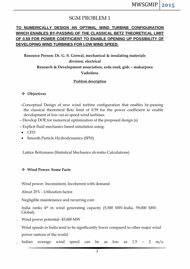
India ranks 4th in wind generating capacity (5,500 MW-India, 59,000 MW- Global).

Wind power potential- 45,000 MW

Wind speeds in India tend to be significantly lower compared to other major wind

power nations of the world.

Indian average wind speed can be as low as 1.5 – 2 m/s.

MWSGMIP 2015

3

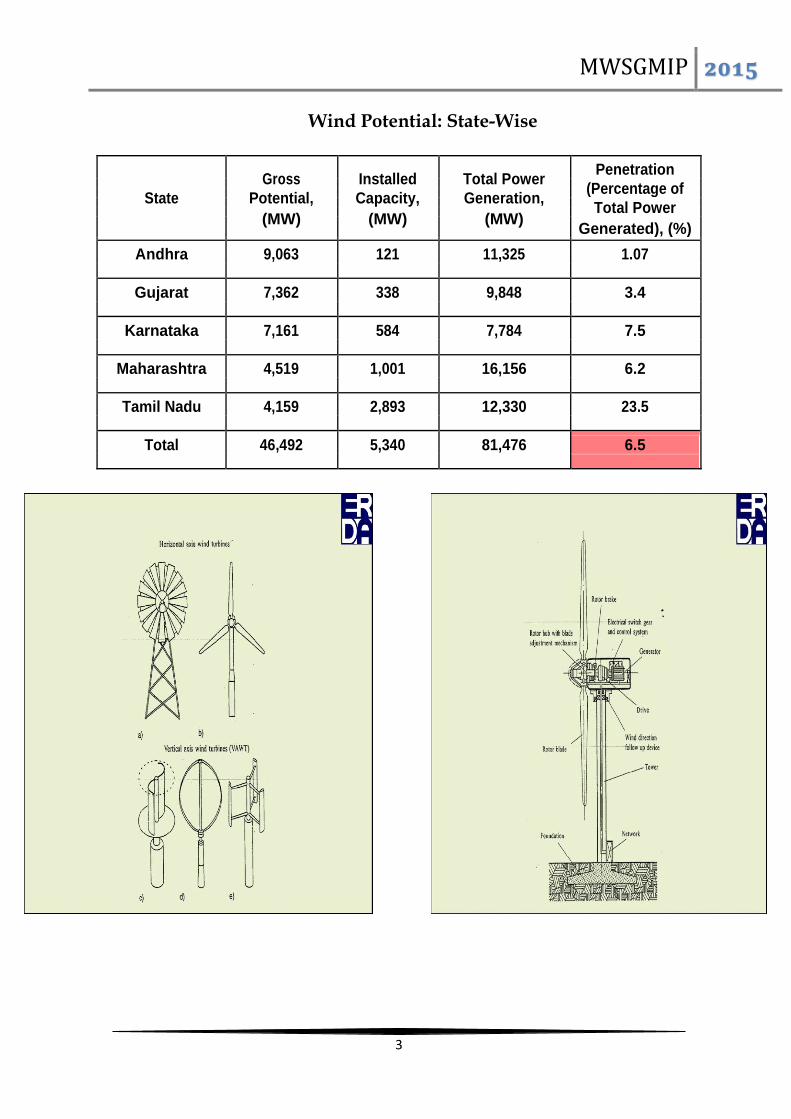
Wind Potential: State-Wise

Gross Installed Total Power

Penetration

(Percentage of

State Potential, Capacity, Generation,

Total Power

(MW) (MW) (MW)

Generated), (%)

Andhra 9,063 121 11,325 1.07

Gujarat 7,362 338 9,848 3.4

Karnataka 7,161 584 7,784 7.5

Maharashtra 4,519 1,001 16,156 6.2

Tamil Nadu 4,159 2,893 12,330 23.5

Total 46,492 5,340 81,476 6.5

MWSGMIP 2015

4

MWSGMIP 2015

5

SGM PROBLEM 2

FINDING PATTERN FREE TRAVESE RATIOS FOR YARN

WINDING

Resource Person: Dr. Milind Koranne,Rajen Patwa,Patwa Kinnariwala Enterprice.

Problem description

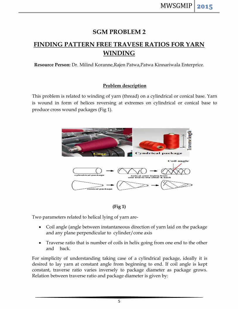
This problem is related to winding of yarn (thread) on a cylindrical or conical base. Yarn

is wound in form of helices reversing at extremes on cylindrical or conical base to

produce cross wound packages (Fig 1).

(Fig 1)

Two parameters related to helical lying of yarn are-

Coil angle (angle between instantaneous direction of yarn laid on the package and any plane perpendicular to cylinder/cone axis

Traverse ratio that is number of coils in helix going from one end to the other and back.

For simplicity of understanding taking case of a cylindrical package, ideally it is desired to lay yarn at constant angle from beginning to end. If coil angle is kept constant, traverse ratio varies inversely to package diameter as package grows. Relation between traverse ratio and package diameter is given by:

MWSGMIP 2015

6

T=2.travese lengthPI.tancoil angle.package diameter

Thus, for a bare cylindrical package of diameter 30 mm with traverse length of 152 mm, filled up to 200 mm traverse ratio varies from 18.2929 to 2.7439 for 10 degree coil angle. During this, it reaches whole numbers (17, 16, 15, 14........ up to 3), half numbers (16 ½, 15 ½, 14 1/2) etc.) one third numbers (17 2/3, 17 1/3, 16 2/3, 16 1/3 ... etc), one fourth, one sixth where yarn reaches its starting point after few repeats and laid one above the other. At such instances, it is not uniformly distributed across its circumference. This phenomenon is known as pattern formation shown in figure 2.

(Fig 2)

Thus, while winding yarn at constant angle, patterning occurs periodically very frequently which is not desired. During change in winding ratio from 18.2929 to 2.7439 mentioned earlier, some traverse ratios do not form pattern where as some form patterns.

This drawback can be avoided as follows. Suppose a package is to be produced with 10 degree coil angle with package dimensions mentioned earlier. We can start winding at bare package with a constant traverse ratio that does not form pattern and gives coil angle closer to 10 degrees. When a package is wound with constant suitable traverse ratio, patterns are not formed but coil angle deceases with increasing package diameter which is not desired. Therefore upon certain build up of the package, if traverse ratio is decreased instantaneously to other lower non-pattern forming traverse ratio, coil angle can be restored back to 10 degree. Thus, at some stage winding starts with new lower value of traverse ratio. Upon continuing winding, again coil angle would decrease that can be again restored back by switching over instantaneously to new lower non-pattern forming ratio.

MWSGMIP 2015

7

PROBLEM HERE IS HOW TO FIND SEREIS OF NON-PATTERN FORMING TRAVESE RATIOS FROM BARE TO FULL PACKAGE WHERE PATTERNS ARE NOT FORMED AND YARN IS DISTRIBUTED HOMOGENEOUSLY ACROSS CICUMFERENCE WITHOUT SEVERAL YARNS BUNCHING CLOSER TO ONE ANOTHER (IN THE EXAMPLE GIVEN, ONE HAS TO FIND AS MANY RATIOS AS POSSIBLE BETWEEN 18.2929 TO 2.7439) SO AS TO MAINTAIN VARIATION OF COIL ANGLE TO MINIUM. YARNS SHOULD BE SEEN AS AN OPEN GRID ON THE PACKAGE.

Parameters here are:

1. BARE & FULL PACKAGE DIAMETERS (FOR CONE THERE WOULD BE TWO DIAMETERS)

2. TAPER OF CONE (For a cylindrical package it is 0 degree)

3. Traverse length

4. Yarn diameter

5. Coil angle

MWSGMIP 2015

8

SGM PROBLEM 3

Measuring PPS (Partial Pixel Shift) in the drift spectrum Generated by Atom Emission Spectrometer

Resource Person: Prof. V. D. Pathak, Dept. of Applied Mathematics, Faculty of Tech. and Engg. ,

The M. S. University of Baroda.

Problem description

An Atom-Emission spectrometer is used to identify the various elements present in a metallic

sample. The metallic sample is placed on a support so that it is exposed to a heat source

generated by igniting an electrode as shown in the figure 1.

Figure 1: Schematic of the Spectrometer

Due to this heat, there will be micro-melting of the sample and an optical signal is generated

which is a combination of signals of various frequencies, ranging from 160 nm to 410 nm

depending on elements present in the sample. This optical signal is projected on a holographic

diffraction grating through an entrance slit. This diffraction element splits the composite light source

into spectral components. Then a transducer is used to convert the optical information to an

electrical signal, which is captured in the analogue form. whose resolution depends on the

pixel configuration of the CCD used in the system. The various peaks observed in a signal are

then compared with the known responses of the standard samples having known composition

of elements and the given sample is analyzed on the basis of this comparison. The

interpretation depends on how accurately these peaks are identified. It is possible that the

actual peak or height of the line information (counts) is not the same as the maximum peak

MWSGMIP 2015

9

observed by the CCD, i. e. the actual peak is missed out due to the peak falling on the gap

between two pixels.

There may be other reasons due to which the peak line information is not obtained correctly.

For example, due to some functional deficiencies in the spectrometer the spectrum of test

sample (drift spectrum) shifts relative to the spectrum of the reference sample (reference

spectrum) and hence the pixel positions of the peaks in the test sample shift from their true

positions. These shifts can be by 1, 2, .. pixels or even by partial pixels. Also the counts

corresponding to these peaks may change in the drift spectrum.

Our problem is to identify the Partial pixel shifts (PPS) in each of the required elements i. e.

peak positions corresponding to these elements and then correct PPS for the elements. Also,

make the corresponding count corrections.

Finding full pixel shifts is relatively simple and is regularly done by the Industry. However,

identifying and correcting partial pixel shift (PPS) is an important issue for which the problem

was referred to us. Thus the main task is to:

Calculate PPS in the Drift spectrum w.r.t. to reference spectrum. Drift spectrum is the partially or

fully shift spectrum.

MWSGMIP 2015

10

Following are the spectrum Data:

1. Reference spectrum from Pixel position 3350 to 3450:

2. Drift spectrum from Pixel position 3350 to 3450:

MWSGMIP 2015

11

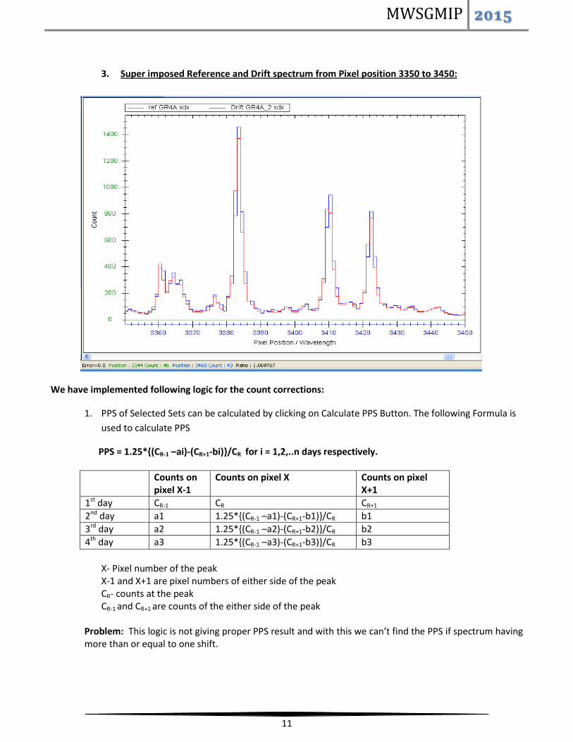
3. Super imposed Reference and Drift spectrum from Pixel position 3350 to 3450:

We have implemented following logic for the count corrections:

1. PPS of Selected Sets can be calculated by clicking on Calculate PPS Button. The following Formula is

used to calculate PPS

PPS = 1.25*{(CR-1 –ai)-(CR+1-bi)}/CR for i = 1,2,..n days respectively.

Counts on pixel X-1

Counts on pixel X Counts on pixel X+1

1st day CR-1 CR CR+1

2nd day a1 1.25*{(CR-1 –a1)-(CR+1-b1)}/CR b1

3rd day a2 1.25*{(CR-1 –a2)-(CR+1-b2)}/CR b2

4th day a3 1.25*{(CR-1 –a3)-(CR+1-b3)}/CR b3

X- Pixel number of the peak X-1 and X+1 are pixel numbers of either side of the peak CR- counts at the peak CR-1 and CR+1 are counts of the either side of the peak

Problem: This logic is not giving proper PPS result and with this we can’t find the PPS if spectrum having more than or equal to one shift.

MWSGMIP 2015

12

SGM PROBLEM 4

VLE PREDICTION USING HR-SAFT MODEL

Resource Person: Bharat doshi,Vinayak Organics Pvt. Ltd., Waghodia(bharatdoshi1950@gmail.com )

and Dr. Nitin Bhate, Dept. of Chemical Engineering,

The M. S. University of Baroda.

Problem description

Distillation is one of the most commonly used unit operations in Chemical Industry. This may be used

to either for separation of liquids by the virtue of their boiling points or for solvent recovery. Efficient

design of distillation system requires authentic vapour-liquid equilibrium (VLE) data and robust

models. Many a times the conventional models fail to predict VLE leading to inefficient design of

distillation columns. Due to this the product quality is hampered. Use of alternate (non-conventional)

models like HR-SAFT EOS may help to address this issue. Our industry is involved in the separation of

multi-component systems by distillation. A sound understanding and validity of such models can

significantly help our industry to improvise the quality and optimize the energy required for the

distillation operation. HR-SAFT EOS is highly non-linear and complex in nature. Moreover, the overall

expression has a power of ‘9’ which makes the solution extremely challenging. Also in the process of

solving the equations some parameters need to be estimated. This makes it a multi-regression problem.

MWSGMIP 2015

13

Expectations:

Numerical approach to determine the vapour pressure of polar and non-compounds and estimate the

parameters of binary and multi-component systems. Validation of these models with the existing data.

The proposed algorithm for solving the above problem is given below:

MWSGMIP 2015

14

VAPOUR PRESSURE & PARAMETER ESTIMATION OF PURE COMPONENT USING HR-SAFT

EOS

(Non Associating Component)ALGORITHM :

Bm

START

Select the Component

Read Pure Component Parameters

m, ν00, u0/k, KAB, εAB/k

Specify the Temperature T

Calculate Temperature Dependent parameters σ,

ν0,u/kT using equations (1),(2),and (3)

Guess ηL and ηV such that ηL > ηV

Change ηL and ηV

Increase ηL Decrease ηL

Calculate Zseg, Zchain, Zassoc for liquid and vapor using

equations (20),(21),and (22) resp.

1

A

MWSGMIP 2015

15

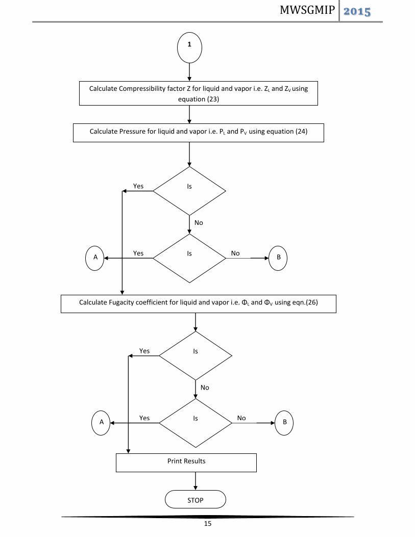
1

Calculate Compressibility factor Z for liquid and vapor i.e. ZL and ZV using

equation (23)

Calculate Pressure for liquid and vapor i.e. PL and PV using equation (24)

Is

PL= PV?

No

Is

PL> PV?

No

Yes

Yes

Calculate Fugacity coefficient for liquid and vapor i.e. ΦL and ΦV using eqn.(26)

Is

ΦL= ΦV?

No

Is

ΦL> ΦV?

No

Yes

Yes

Print Results

STOP

A B

A B

MWSGMIP 2015

16

Equations used:

1. Select Component

2. Specify System Temperature (K)

3. Read following parameters from Segment data bank and Parameter data bank

Molar mass Temp. range Segment Vol. Segment Dispersion Energy

MM T range, K voo, mL/mol uo/k, K

Voo, m3/mol

Segment Number Association Energy Association Vol. Association Vol.

m ϵAB/k, K 102KAB KAB

4. Take Mole fraction Xi and Yi = 1 for Pure Components.

5. Constants:

Gas constant R = 0.00008314 (bar m3/mol K)

Tau τ = 0.74048

Integration const C= 0.12

Nav = 6.023E+23 (1/mole)

Boltzmann constant k = 1.38E-23 (J/K)

6. Assume η for Liquid and Vapour such that ηL > ηV

η Upper Limit Lower Limit Starting value

η liq 0.5 9.00E-03 5.00E-01

η vap 0.009* 1.00E-10 1.00E-04

Yes

MWSGMIP 2015

17

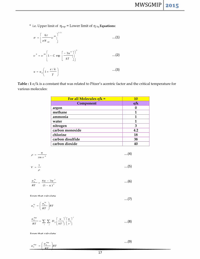
* i.e. Upper limit of ηvap = Lower limit of η liq Equations:

Table : 1 e/k is a constant that was related to Pitzer’s acentric factor and the critical temperature for

various molecules:

For all Molecules e/k = 10

Component e/k

argon 0

methane 1

ammonia 1

water 1

nitrogen 3

carbon monoxide 4.2

chlorine 18

carbon disulfide 38

carbon dioxide 40

3/1

006

AVN

30

000 3exp1

kT

uC

T

keuu

/1

0

….(1)

….(2)

….(3)

0

m

1V

2

2

0

)1(

34

RT

ahs

….(4)

….(6)

….(5)

RTRT

aa

hs

hs

0

0

ji

i j

ij

disp

kT

uD

RT

a

0

….(8)

RTRT

aa

disp

disp

0

0

….(9)

From that calculate

From that calculate

From that calculate

From that calculate

….(7)

MWSGMIP 2015

18

Table -2 Dij’s – Universal constants for HR-SAFT

Dij’s – Universal constants proposed by Chen and Kreglewski (1977) used for the dispersion term in

HR-SAFT. Dij : i =1 to 4 and j = 1 to 9

i j

1 2 3 4

1 -8.8043 2.9396 -2.8225 0.34

2 4.164627 -6.0863583 4.7600148 -3.1875014

3 -48.203555 40.137956 11.257177 12.213796

4 140.4362 -76.230797 -66.382743 -12.110681

5 -195.23339 -133.70055 69.248785 0

6 113.515 860.25349 0 0

7 0 -1535.3224 0 0

8 0 1221.4261 0 0

9 0 -409.10539 0 0

….(10) 3

)1(

2

11

ln)1(

mRT

achain

RTRT

aa

chain

chain

disphssegaaa

000

segsegmaa

0

assocchainsegresaaaa

….(11)

….(13)

….(12)

….(14)

RTa

RT

a res

res1

….(15)

Take aassoc = 0 for Non Associating Components

From that Calculate

MWSGMIP 2015

19

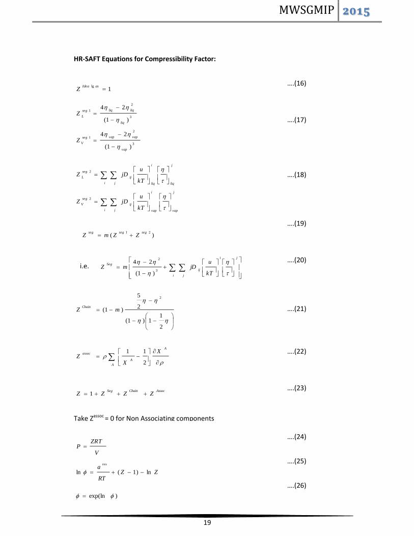
HR-SAFT Equations for Compressibility Factor:

1lg

asIdea

Z

3

2

1

3

2

1

)1(

24

)1(

24

vap

vapvapseg

V

liq

liqliqseg

L

Z

Z

j

vap

i

vapi j

ij

seg

V

j

liq

i

liqi j

ij

seg

L

kT

ujDZ

kT

ujDZ

2

2

)(21 segsegseg

ZZmZ

i j

ji

ij

Seg

kT

ujDmZ

3

2

)1(

24i.e.

2

11)1(

2

5

)1(

2

mZChain

AssocChainSegZZZZ 1

Take Zassoc = 0 for Non Associating components

V

ZRTP

ZZRT

ares

ln)1(ln

)exp(ln

….(16)

….(20)

….(19)

….(21)

….(18)

….(22)

….(23)

….(17)

A

A

A

assoc X

XZ

2

11

….(24)

….(25)

….(26)

MWSGMIP 2015

20

NOMENCLATURE

HR-SAFT

a = molar Helmholtz energy (total, res, seg, bond, assoc. etc.) per

mole of molecules

a0 = segment molar Helmholtz energy (seg), per mole of segments

C = integration constant in eq.(2)

d = temperature-dependent segment diameter, Ǻ

elk = constant in eq. (3)

k = Boltzmann's constant = 1.381 X 10 -23 J/K

m = effective number of segments within the molecule

(segment number)

mυ 00 = volume occupied by 1 mole of molecules in a close- packed

arrangement, mL/mol

M = number of association sites on the molecule

MM = molar mass, g/mol

Molar = molar with respect to molecules

N = total number of molecules

NAv = Avogadro's number = 6.02 X 10 23 molecules / mole

P = pressure

Pc = critical pressure, bar

MWSGMIP 2015

21

P sat = saturated vapor pressure

R = gas constant

Segment molar = molar with respect to segments

T = temperature, K

Tc = critical temperature, K

u/k = Temperature-dependent dispersion energy of interaction

between segments, K

u0/ k = Temperature-independent dispersion energy of inter- action between segments, K

V = molar volume, m3/mol

V liq = liquid molar volume, mL/mol of bulk fluid

υ0 = temperature-dependent segment volume, mL/mol of segments

υ00 = temperature-independent segment volume, mL/mol of segments

X = mole fraction

XA = monomer mole fraction (mole fraction of molecules NOT

bonded at site A)

Z = P V / (RT), compressibility factor

KAB = volume of interaction between sites A and B

∆AB = strength of interaction" between sites A and B, Å3

εAB/ k = association energy of interaction between sites A and B, K

η = ( лNAv / 6) ρ md3, pure component reduced

density, the same for segments AND molecules

ρ = ρn / NAv molar density, mol/Å3

ρn = number density (number of molecules in unit volume), Å-3

MWSGMIP 2015

22

σ = Lennard-Jones segment diameter (temperature independent), Å

A

= summation over all the sites (starting with A)

τ = close-packed reduced density =0.74048

Superscripts :

A, B, C, D, ... = association sites

res = residual

seg = segment

assoc = associating, or due to association

hs = hard sphere

ideal = Ideal gas

1. Determination of vapor pressure and Fugacity coefficient of n-Hexane using known parameters

Data:

Molar mass MM = 86.178

T range= 243-493 K

Segment volume voo = 12.475 mL/mol =0.000012475 m3/mol

Segment Number m = 4.724

Segment Dispersion Energy uo/k = 202.72 K

Mole Fraction Xi = 1 and Yi = 1

2. Estimating the parameters of HR-SAFT based on the given P-T data: υ00, m, u0/ k, ηL , ηV.

MWSGMIP 2015

23

SGM PROBLEM 5

MULTI-REGRESSION ANALYSIS OF TERNARY LLE DATA

Resource Person: Gurish Khosala, Deepak Nitrite Ltd., Nandesari(gurishkhosala@deepaknitrite.com) and Dr. Nitin Bhate, Dept. of Chemical Engineering,

The M. S. University of Baroda.

Problem description

Nitration is one of the important unit processes in the Chemical Process Industry. The

products of nitration are used in several applications like explosives, solvents, precursors for

dyes, intermediates and pharmaceuticals. Nitration reaction involves aromatic compound and

a mixture of sulphuric acid and nitric acid. This being a heterogeneous reaction the liquid-

liquid equilibrium (LLE) between the acid and the organic phase becomes important. This

equilibria is highly complex and shows anomalies which do not have a proper explanation till

date.

Our Industry is involved in the nitration of aromatics and substituted aromatics. LLE has

always been a challenge for design of separation equipment and to determine the distribution

of aromatic between the acid and the organic phase. This makes it a ternary system. Usually

the compositions of acid and aromatic in the aqueous (acid) phase are known and the

compositions of acid and water in the organic phase are known. Modeling of this data can help

design of separation systems more efficiently. The challenges in modeling these systems lie in

parameter estimation. This becomes a multi-regression problem since the parameter

estimation is followed by back calculating the above compositions. Parameters are re-

estimated by minimizing the sum of the square of the residuals of predicted and experimental

compositions.

Expectations:

A systematic numerical approach for multi-regression analysis using alternate approaches and

model validation for ternary LLE system.

The equations and the methodology are given here under:

MWSGMIP 2015

24

Parameter estimation and Composition prediction for Ternary LLE using UNIQUAC model

UNIQUAC Model

R

i

C

ii

E

RT

G lnlnln

k

k

k

k

k

k

k

k

kC

kq

z

xx

1ln

21lnln

j

i

iji

kjj

i

ikik

R

kq

ln1ln

i

ii

jj

j

rx

rx

i

ii

jj

j

qx

qx

RT

uuiiji

jiexp

z is the lattice coordination number set equal to 10, xi,= mole fraction, I = activity coefficient,

ij = Binary interaction parameter, ri and qi = volume and surface parameters (known).

Ternary LLE

Criterion for Phase Equilibrium (equations)

1111xx

2222xx

321321)1()1( xxxx

In a ternary system 6 binary interaction parameters have to be regressed (12, 23, 13, 21, 32,

31), 11 = 22 = 33 = 1

MWSGMIP 2015

25

Thus, each data point will lead to 3 equations. There may be 10 to 15 data points (experimental

data) from which the 6 parameters have to be regressed.

Generally,

21, xx and

32, xx are known.

The regressed parameters should be used to back calculate the above compositions and

compare the same with the experimental values

Nitrobenzene: r = 4.07630, q = 3.104

Water: r = 0.92, q = 1.3997

Sulfuric acid: r = 5.65977, q = 5.7848

SGM PROBLEM 6

Temperature Rise In Medium Voltage Switchgear Panels

Resource Person: N. P. Zaveri, Jyoti Ltd., Vadodara.

Problem description

Medium Voltage Switchgear (MV) panels are widely used for distribution of

electrical power in Utilities and Industries. These panels made of sheet metal (2 to

3mm) and house circuit breaker, Current and potential transformers, busbars and

protection and control circuits. The panels typically have three compartments like

Breaker, cable and bus bar compartment. Figure 1 shows typical panel. Panel with

different current rating (eg. 630 Amp to 2000 Amps) are manufactured in the same

basic panel configuration by using appropriate components (breaker, Bus bars,

Current transformers etc.).

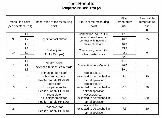
Any MV panel has to pass verification test as per standards and temperature rise

is one such Test. Doc-1 shows typical test configuration. The panel is thermally

insulated on sides allowing heat dissipating only from front, back and top. Also

shown are various temperature measurement points, limiting v/s final

temperature in graphical and tabular form. The bus bar material can be copper or

Aluminum.The possible combinations of bus bar (nos., size, material) are many

and it is not practical to conduct test for every condition. So the test is conducted

with worst possible condition. Say 2x60x10 Al bus bars, top and bottom jumpers

for a breaker rating of say 1250Amp.The same test results are accepted for higher

cross section of bus bar or Copper instead of Aluminum. VCB and self heating are

the primary sources of heat generation

The Problem Statement:

a) If one wants to optimize bus bar & jumper sizes one has to carry out

physical test. In one such experiment for 1250 amp VCB showed that

1x80x10top would work equally well in place of 2x50x10 top jumper with

bus bar of 2x60x10 busbar. This saves 20% material for top jumper. The

question is could there be another such combination. e.g. 1x100x10 bus bar

and 1x80x10 top jumper? Only way would to carry out the test. Such

things are not possible every time due to time and cost consideration.

b) It can beseen that the type test configuration is different from that in actual

panel. The panel used in field has other components e.g. Current

transformers, cables, surge suppressors, CBCT etc. Some of which are heat

source in themselves. Also the panel is never used alone and many such

panels can be coupled together to form board configuration. In such a

situation there are other many heat sources. What would be the

temperature rise at different points in such condition Normal decision is to

derate the panel. The question then is by how much.

c) From the result of the type test it can be seen that there is margin available.

There is a cooling and heating time constant (exponential).To what extent

one can overload the panel in terms of current and time and still be within

specified limits?

Generally decisions in such cases are taken based on experience and thumb

rules.

Desired Result:

There may surely be sophisticated software available for this problem.

However it is desired to simple model using generally available software.

The model could be tailored to specific configuration based on few physical

experiments to be conducted. What physical experiments to conduct to be

enumerated?

Could the model be self refining as more and more actual data is added to

the data base.

The model need not be very accurate as out put can be used as figure of

merit to get optimized solution to be followed by physical verification.

Test Arrangement and Measuring Points for

Temperatures and Resistances of Panels and Busbar

11

expanded expanded polystyrene polystyrene 30 mm 30 mm

Feeder Panel PH-800F 1250 A

Measuring points (L1, L2, L3)

Measuring Points for Temperatures and Resistances

of Feeder Panel / PH-800F

10 8 4

14

15

9

3

1 2

1x60x10mm2 Cu

13

12

Measuring points (L1, L2, L3)

Measuring points (accessible parts)

Measuring Points for Temperatures and Resistances

of Vacuum Circuit-Breaker / VK-10M25F

7 8

6

5

4 Measuring points (L1, L2, L3)

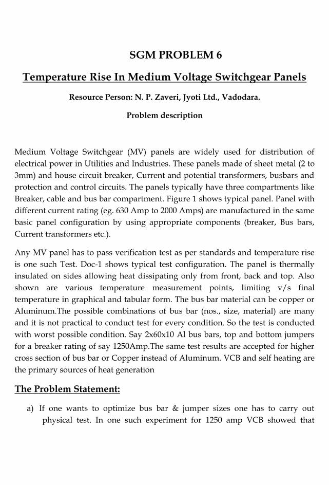
Test Results Temperature-Rise Test (2)

Final Permissible

Measuring point Description of the measuring Nature of the measuring temperature temperature

(see sheets 9 – 11) point point rise rise

K K

L1 Connection, bolted, Cu, 47.1

silver coated in air in

9 L2 Upper contact shroud 46.2 75

contact with insulation

L3

material class E 46.9

10 L1

Busbar joint Connection, bolted, Cu, 43.8

75

L2 42.1

(T-off / Dropper) silver coated in air

L3 42.1

11 L1

Neutral point Connection bare Cu in air

41.1 -

L2 40.7

extended busbar, left outside

L3

39.1

Handle of front door Accessible part

12 - c.b. compartment expected to be touched in 3.4 30

Feeder Panel / PH-800F normal operation

Front door Accessible part

13 - c.b. compartment top expected to be touched in 6.5 30

Feeder Panel / PH-800F normal operation

14 - Front plate Accessible part

b.b. compartment top expected to be touched in 9.6 30

Feeder Panel / PH-800F normal operation

15 - Rear cover top Accessible part

expected to be touched in 7.6 30

Feeder Panel / PH-800F

normal operation

SGM PROBLEM 7

MODELING AND PREDICTION OF COAL

PULVERISER PERFORMANCE

Resource person: Nagesh Patki, E&, L&T Power, NH-8, Ajwa Waghodia crossing, Vadodara –

3900019.

nrp@lntpower.com

Introduction Coal Pulveriser or coal mill play a very important role in the performance & reliability of any sub-

critical or supercritical coal based power plant. Mill grinds coal into fine particle and hence enables

it to be burnt like gas in boilers for more efficient combustion. Fine coal particle are transported by

combustion air (primary air) as gas-solid mixture to boiler. Typically there are six mills in a large

sized coal based power plant. Coal fired power stations are required to operate more flexibly with

more varied coal specifications. The power stations are also required to vary the output in

response to the changes of electricity demands. To meet varied demand, there are frequent load

changes, start-up and shutdown of the mills which create transients and deterioration of mill

availability and performance. Poor performance of the coal mill will lead to decrease in the overall

efficiency of the power plant besides their own failure. Hence it is necessary to model and develop

suitable scheme to ensure optimum control of the coal mills

Problem Definition During load change, transients are created in mills loading. Many times the mill which is already

loaded gets loaded more during transient conditions. Due to this, coal fineness and mill availability

gets affected. Ideally, all the mills should be loaded equally. There is therefore requirement of

‘coordinated control’ between the mills for their optimal performance and loading. A mathematical

model is required to predict mill performance parameters with input of actual measured operating

values. Control systems can be designed which will utilise the mathematical model to control

various mill parameters during the load changes.

Typical Measured Parameters in Coal Mill Typically following parameters are measured in a coal mill.

a) Coal feeder speed b) Primary air differential pressure c) Primary air temperature d) Mill differential pressure e) Coal Mill Inlet & Outlet temperature f) Mill motor current

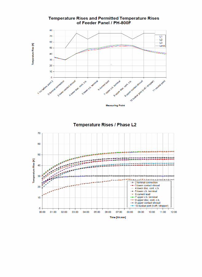
Model Governing Equations A typical coal mill is shown in Figure-1. Following governing equations are given below for coal mill

modelling. 1: Computation of primary air flow Wair to mill Direct measurement of flow of primary air to mills is not possible. In indirect method we can have

data of primary air differential pressure (mbar) Δppa and also inlet temperature of coal mill Tin.

Wang1 etc have proposed a semi-empirical relationship as given below.

Wair 10 pa (t). 360

(1)

273 Tin (t)

Figure 1: Schematic diagram of coal mill 2: Coal inlet mass flow rate (Wc (t)) as function of feeder speed FS (t)

Wc (t) K fs Fs (t) (2) The feeder coefficient Kfs depends upon size of the feeder. For large feeders Kfs =0.24 kg/mm. Modern power plant coal feeders are provided with strain gage based measurement. In case

details are made available, equation 2 gets modified with direct read-out of Wc(t) and thus

parameters such as Kfs and Fs (t) would disappear in mathematical model. 3: Computation of flow rate of pulverized fuel (PF) This is the flow rate of pulverized coal carried out of the mill by primary air flow. This is

proportional to mass of pulverized coal in the mill and the differential pressure produced by

primary air fan. This includes the actual out flow from the mill and mass of particles rejected by

classifier for regrinding them to sizes accepted by classifier. The equation is

Wpf (t) K16 Ppa (t)M pf (t) (3)

It is very convenient to identify certain model coefficients (Ki) which can be evaluated by using

operational data analyzed using advanced computational methods such as differential evolution or

similar algorithms. In the analysis of mill we shall come across about 16 model coefficients. It is

necessary to follow such approach as it is impossible to solve differential equations resulting from

rigorous mathematical analysis.

4: Computation of Mass Flow Rate

(t) of Pulverized Coal in Mill

M c

(t) Wc (t) k15M c (t)

(4)

M c

WC is mass flow rate of coal into mill (kg/sec). This data comes from coal feeder instrumentation k15 is model coefficient related to inflow of raw coal and amount of coal pulverized which contains

classifiable and unclassifiable pulverized coal. In an ideal situation the entire pulverized mass

should contain size fractions which will pass through classifier. In actual practice, however some

portion of pulverized mass returns to bowl for further grinding. 5: Rate of Pulverized Coal Mass Flow

(t) k15M c (t) Wpf (t) (5)

M pf

Mpf is mass of pulverized coal in the mill (kg) Wpf is mass flow rate of pulverized coal outlet from mill (kg/sec) while Mc is mass of coal in mill (kg). 6: Mill Current (P (t)) The mill current is one parameter which can be accurately measured as well as continuously

monitored. It depends upon mass of pulverized coal M pf , mass Mc of coal in mill. The equation is

P(t) k6 M pf (t) k7 M c (t) k8 (6)

The constants kt and k8 must be determined using operating and are mill/site specific. 7: Relation between Mill Differential, Primary Air Differential Pressure and Mill Product Differential Pressure

Pmill (t) k9 Ppa (t) Pmpd (t) (7) 8: Relation between Mill Product Differential Pressure, Mass of Pulverized Coal in Mill, Mass of Coal in Mill

(t) k11M pf (t) k12 Mc (t) k13 Pmpd (t) (8)

Pmpd

The k’s in above equations are constants which are evaluated from analysis of operating data. 9: Relation of Mill Outlet Temperature

Tout (t) [k1Tin (t) k2 ]Wair (t) k3Wc (t) [k4Tout (t) k5 ].[Wair (t) Wc (t)] k14 P(t) k1Tout (t) (9) This equation represents the changes in mill outlet temperature. It includes heat contribution by

hot primary air entering mill and the heat generated by grinding. It also includes heat loss in drying

of coal and other miscellaneous losses.

inlet.heat.coal Qout k3WC

pa.heat k1Tin k2Wair

heat, grinding k14 P heat.pc [k4Tout (t) k5 ].[Wair (t) Wc (t)]

The rigorous analysis of energy transfer is done in next section.

Energy Balance Model of Coal Mill Figure 3 is illustration of energy balance in the mill. T is the temperature in the mill, Qair is the

energy of primary air flow, Pmotor denotes the power used to crush the coal, Qcoal is the energy in

the coal flow and Qmoisture is the energy in the coal moisture.

Figure 3: Energy balance in the mill

To begin with, let us assume that quantity of ground coal delivered to boiler is equal coal supplied

to mill for grinding. This of course is valid for steady state and with assumption to simplify the

model. The energy balance is given by

(t) Qcoal (t)

Qmoisture

(t)

Pmotor (1)

mmCmT (t) Qair

The heating and evaporation of moisture in coal is modelled by a combined heating coefficient.

The temperature, with loop control is kept as 1000 C. the latent heat of evaporation dominates the

energy required for heating of moisture by few degrees. The combined heat coefficient Hst is defined as

H

st Cw Lsteam /100, (2)

Cw specificheatofwater

We may now write the model equation as

mmCmT

(t)

(t) mpa (t)Cair (Tpa (t) T (t)) mc (t)Cc (Ts T (t)) (t)mc (t)CwTs (t)mc (t)HstT (t) Pmotor

(10)

Cm is specific heat of the mill, T(t) is mill temperature at classifier,

(t) is mass flow rate of

mpa

(t) is coal mass rate, (t) is ratio of moisture, Cw is specific

primary air, Cc is specific heat of coal, mc

heat of moisture.

Identification of system For the purpose of identifying the system parameters, the measured variables are organized in two

groups. Group 1 includes system inputs and group 2 consists of system outputs. The input variables are (1)

coal flow in the mill, (2) primary air differential pressure and (3) primary air temperature. The output variables are (1) mill differential pressure, (2) outlet temperature and (3) mill current. There are sixteen unknown coefficients (k1.........k16). These can be evaluated using Genetic Algorithms (GA’s)

GA is a robust optimization method for identification of the unknowns as described above. This

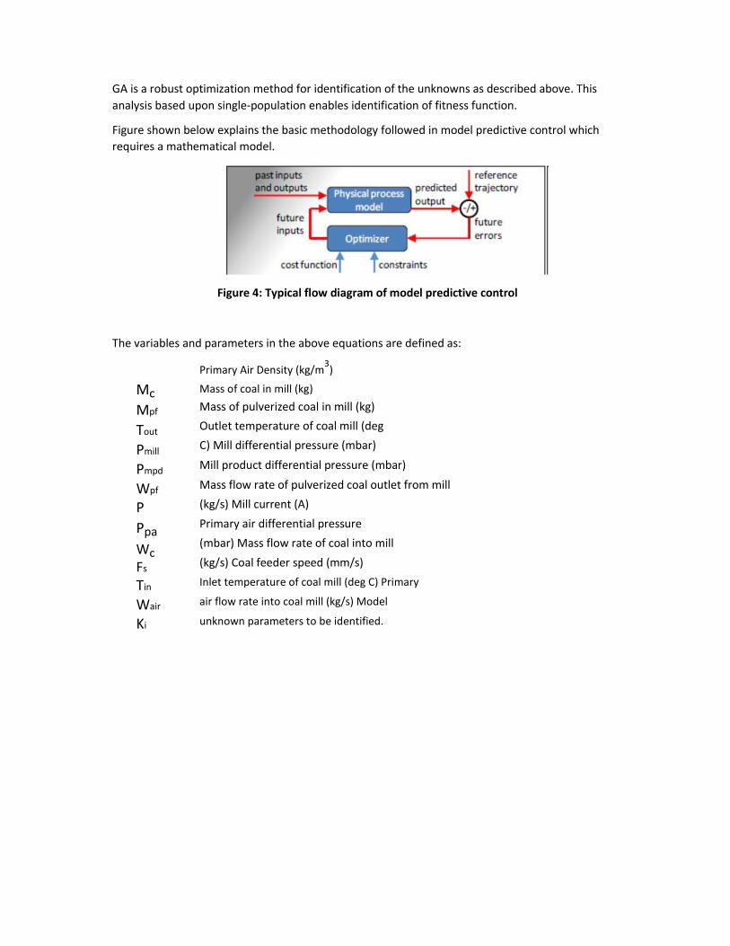
analysis based upon single-population enables identification of fitness function. Figure shown below explains the basic methodology followed in model predictive control which

requires a mathematical model.

Figure 4: Typical flow diagram of model predictive control

The variables and parameters in the above equations are defined as:

Mc Mpf Tout

Pmill

Pmpd

Wpf P

Ppa

Wc Fs

Tin Wair

Ki

Primary Air Density (kg/m

3)

Mass of coal in mill (kg) Mass of pulverized coal in mill (kg)

Outlet temperature of coal mill (deg

C) Mill differential pressure (mbar) Mill product differential pressure (mbar) Mass flow rate of pulverized coal outlet from mill

(kg/s) Mill current (A) Primary air differential pressure

(mbar) Mass flow rate of coal into mill

(kg/s) Coal feeder speed (mm/s) Inlet temperature of coal mill (deg C) Primary

air flow rate into coal mill (kg/s) Model

unknown parameters to be identified.

MWSGMIP 2015

SGM PROBLEM 8

SENSOR-LESS VECTOR CONTROL OF INDUCTION MOTOR

Resource Person: Amtech_Industry Problem

Problem description

Product: AC variable frequency drive Application: Speed control of AC induction motor Type of control: Field oriented sensor-less vector control

We are using ac variable frequency drive for different industrial application like pump, fan, hoist, crain, conveyor, pump jack, paper automation etc.. In some applications, we require better torque and speed control at low speed, which can not be achieved by V/F control method. Such applications require vectrol control mode in variable frequency drive.

For vectrol control, the essential reqiurement is to have an exact mathematical motor model and motor parameter otherwise the performance of the system can be worse than V/F mode. It is not possible to get the motor parameters from motor name plate or by external measurement by any instrument. It is expected that the modern VFD identify motor parameters by "Self Comminsionig" or "Autotunning" or "Motor parmeter Identification mode" like functions. For that they use, TI- type mathematical model for induction motor and motor parameter are shown below.

Where,

R1 = Primary resistance = Stator resistance (Ohm) L6 = Leackage inductance (Henry) M' = Mutual inductance = Exitation inductance (Henry) R2' = Secondary resistance = Rotor resistance (Ohm)

There are various papers published describing different methods to find out the above parameters. One is as mentioned below.

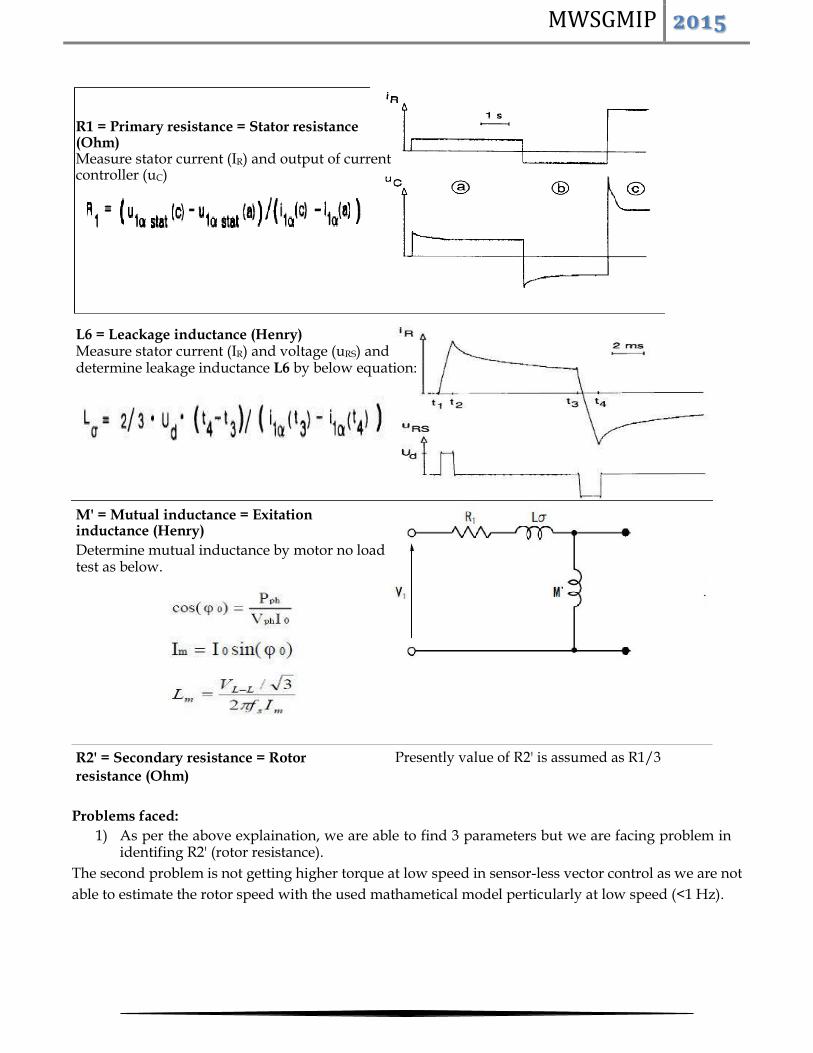
MWSGMIP 2015

R1 = Primary resistance = Stator resistance (Ohm) Measure stator current (IR) and output of current controller (uC)

L6 = Leackage inductance (Henry) Measure stator current (IR) and voltage (uRS) and determine leakage inductance L6 by below equation:

M' = Mutual inductance = Exitation inductance (Henry) Determine mutual inductance by motor no load test as below.

R2' = Secondary resistance = Rotor Presently value of R2' is assumed as R1/3

resistance (Ohm)

Problems faced:

1) As per the above explaination, we are able to find 3 parameters but we are facing problem in identifing R2' (rotor resistance).

The second problem is not getting higher torque at low speed in sensor-less vector control as we are not

able to estimate the rotor speed with the used mathametical model perticularly at low speed (<1 Hz).

MWSGMIP 2015