Problem Set IV: UMP, EMP, indirect utility, expenditure

Paolo Crosettopaolo.crosetto@unimi.it

February 22nd, 2010

Recap: indirect utility and marshallian demand

• The indirect utility function is the value function of the UMP:

v(p,w) = max u(x) s.t. p · x ≤ w

• Since the end result of the UMP are the Walrasian demand functions x(p,w),

• the indirect utility function gives the optimal level of utility as a function ofoptimal demanded bundles,

• that is, ultimately, as a function of prices and wealth.

Summing up

• In the UMP we assume a rational and locally non-satiated consumer withconvex preferences that maximises utility;

• we hence find the optimally demanded bundles at any (p,w);

• The level of utility associated with any optimally demanded bundle is theindirect utility function v(p,w).

2 of 30

Recap: properties of the indirect utility function

The value function of a standard UMP, the indirect utility function v(p,w), is:

• Homogeneous of degree zero in p and w (doubling prices and wealth doesn’tchange anything);

• Strictly increasing in w and nonincreasing in pl for any l (all income is spent;law of demand);

• Quasiconvex in p: that is, {(p,w) : v(p,w) ≤ v} is convex for any v (seeexample in R2 in lecture slides);

• Continuous at all p � 0, w > 0 (from continuity of u(x) and of x(p,w)).

3 of 30

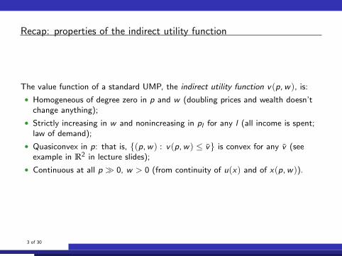
Cobb-Douglas Indirect Utility Function, α = 0.5, w = 100

0

50

100

0

50

100

1

2

3

4

5

4 of 30

Recap: expenditure function and hicksian demand

• The expenditure function is the value function of the EmP:

e(p, u) = min p · x s.t. u(x) ≥ u

• In the EmP we find the bundles that assure a fixed level of utility whileminimizing expenditure

• the expenditure function gives the minimum level of expenditure needed toreach utility u when prices are p.

Summing up

• In the EmP we assume a rational and locally non-satiated consumer withconvex preferences that minimises expenditure to reach a given level of utility;

• we denote the optimally demanded bundles at any (p, u) as h(p, u) [hicksiandemand];

• The level of expenditure associated with any optimally demanded bundle is theexpenditure function e(p, u).

5 of 30

Recap: properties of the expenditure function

• Homogeneous of degree one in p (expenditure is a linear function of prices);

• Strictly increasing in u and nondecreasing in pl for any l (you spend more toachieve higher utility, you cannot spend less when prices go up);

• Concave in p (consumer adjusts to changes in prices doing at least not worsethan linear change);

• Continuous in p and u (from continuity of p · x and h(p, u)).

6 of 30

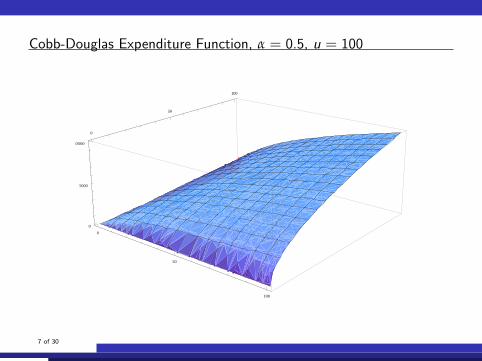
Cobb-Douglas Expenditure Function, α = 0.5, u = 100

0

50

100

0

50

100

0

5000

10 000

7 of 30

Recap: basic duality relations

• The bundle that maximises utility is the same that minimises expenditure

• The indirect utility function gives the maximum utility obtainable with thatbundle

• The wealth spent to obtain that utility is necessarily the minimum possible

• And spending all that wealth generates the maximum level of utility.

Four important identities

1. v(p, e(p, u)) ≡ u: the maximum level of utility attainable with minimalexpenditure is u;

2. e(p, v(p,w)) ≡ w : the minimum expenditure necessary to reach optimal levelof utility is w ;

3. xi (p,w) ≡ hi (p, v(p,w)): the demanded bundle that maximises utility is thesame as the demanded bundle that minimises expenditure at utility v(p,w);

4. hi (p, u) ≡ xi (p, e(p, u)): the demanded bundle that minimises expenditure isthe same as the demanded bundle that maximises utility at wealth e(p, u).

8 of 30

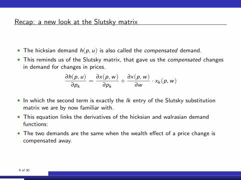
Recap: a new look at the Slutsky matrix

• The hicksian demand h(p, u) is also called the compensated demand.

• This reminds us of the Slutsky matrix, that gave us the compensated changesin demand for changes in prices.

∂h(p, u)

∂pk=

∂x(p,w)

∂pk+

∂x(p,w)

∂w· xk (p,w)

• In which the second term is exactly the lk entry of the Slutsky substitutionmatrix we are by now familiar with.

• This equation links the derivatives of the hicksian and walrasian demandfunctions:

• The two demands are the same when the wealth effect of a price change iscompensated away.

9 of 30

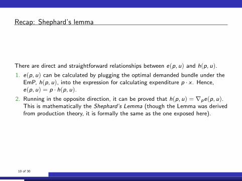
Recap: Shephard’s lemma

There are direct and straightforward relationships between e(p, u) and h(p, u).

1. e(p, u) can be calculated by plugging the optimal demanded bundle under theEmP, h(p, u), into the expression for calculating expenditure p · x . Hence,e(p, u) = p · h(p, u).

2. Running in the opposite direction, it can be proved that h(p, u) = ∇pe(p, u).This is mathematically the Shephard’s Lemma (though the Lemma was derivedfrom production theory, it is formally the same as the one exposed here).

10 of 30

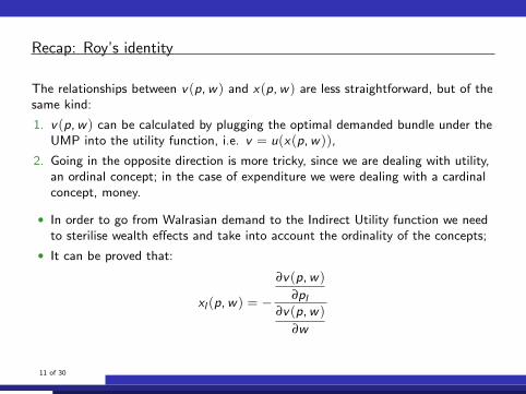
Recap: Roy’s identity

The relationships between v(p,w) and x(p,w) are less straightforward, but of thesame kind:

1. v(p,w) can be calculated by plugging the optimal demanded bundle under theUMP into the utility function, i.e. v = u(x(p,w)),

2. Going in the opposite direction is more tricky, since we are dealing with utility,an ordinal concept; in the case of expenditure we were dealing with a cardinalconcept, money.

• In order to go from Walrasian demand to the Indirect Utility function we needto sterilise wealth effects and take into account the ordinality of the concepts;

• It can be proved that:

xl (p,w) = −

∂v(p,w)

∂pl∂v(p,w)

∂w

11 of 30

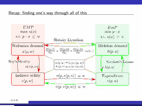
Recap: finding one’s way through all of this

12 of 30

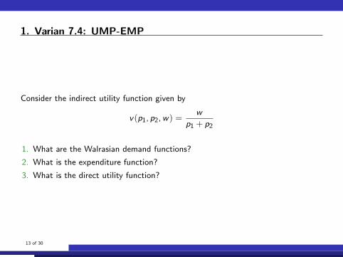
1. Varian 7.4: UMP-EMP

Consider the indirect utility function given by

v(p1, p2,w) =w

p1 + p2

1. What are the Walrasian demand functions?

2. What is the expenditure function?

3. What is the direct utility function?

13 of 30

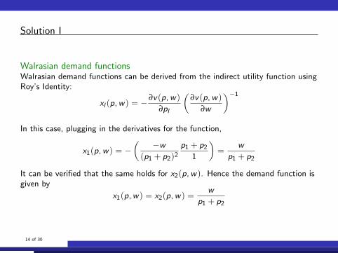
Solution I

Walrasian demand functionsWalrasian demand functions can be derived from the indirect utility function usingRoy’s Identity:

xl (p,w) = − ∂v(p,w)

∂pl

(∂v(p,w)

∂w

)−1

In this case, plugging in the derivatives for the function,

x1(p,w) = −(

−w(p1 + p2)2

p1 + p2

1

)=

w

p1 + p2

It can be verified that the same holds for x2(p,w). Hence the demand function isgiven by

x1(p,w) = x2(p,w) =w

p1 + p2

14 of 30

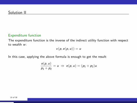
Solution II

Expenditure function

The expenditure function is the inverse of the indirect utility function with respectto wealth w :

v(p, e(p, u)) = u

In this case, applying the above formula is enough to get the result:

e(p, u)

p1 + p2= u ⇒ e(p, u) = (p1 + p2)u

15 of 30

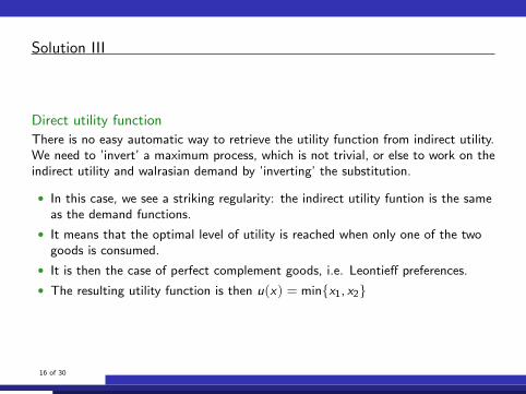
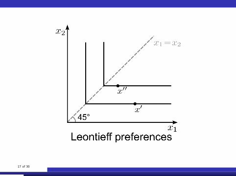
Solution III

Direct utility function

There is no easy automatic way to retrieve the utility function from indirect utility.We need to ’invert’ a maximum process, which is not trivial, or else to work on theindirect utility and walrasian demand by ’inverting’ the substitution.

• In this case, we see a striking regularity: the indirect utility funtion is the sameas the demand functions.

• It means that the optimal level of utility is reached when only one of the twogoods is consumed.

• It is then the case of perfect complement goods, i.e. Leontieff preferences.

• The resulting utility function is then u(x) = min{x1, x2}

16 of 30

17 of 30

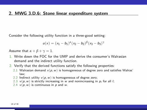
2. MWG 3.D.6: Stone linear expenditure system

Consider the following utility function in a three-good setting:

u(x) = (x1 − b1)α(x2 − b2)

β(x3 − b3)γ

Assume that α + β + γ = 1.

1. Write down the FOC for the UMP and derive the consumer’s Walrasiandemand and the indirect utility function.

2. Verify that the derived functions satisfy the following properties:2.1 Walrasian demand x(p,w ) is homogeneous of degree zero and satisfies Walras’

law;2.2 Indirect utility v (p,w ) is homogeneous of degree zero;2.3 v (p,w ) is strictly increasing in w and nonincreasing in pl for all l ;2.4 v (p,w ) is continuous in p and w .

18 of 30

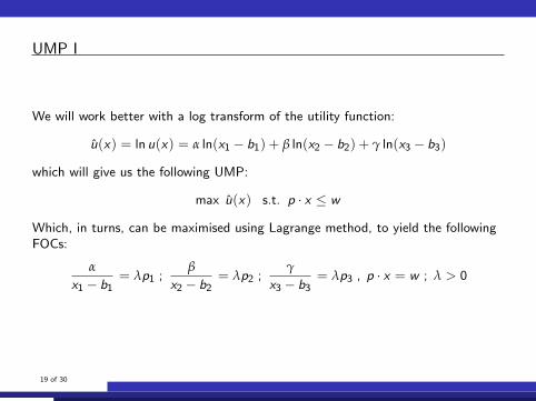
UMP I

We will work better with a log transform of the utility function:

u(x) = ln u(x) = α ln(x1 − b1) + β ln(x2 − b2) + γ ln(x3 − b3)

which will give us the following UMP:

max u(x) s.t. p · x ≤ w

Which, in turns, can be maximised using Lagrange method, to yield the followingFOCs:

α

x1 − b1= λp1 ;

β

x2 − b2= λp2 ;

γ

x3 − b3= λp3 , p · x = w ; λ > 0

19 of 30

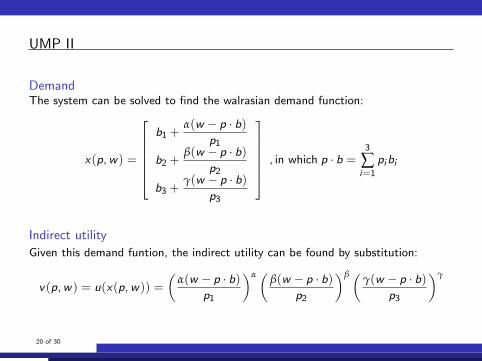
UMP II

DemandThe system can be solved to find the walrasian demand function:

x(p,w) =

b1 +

α(w − p · b)p1

b2 +β(w − p · b)

p2

b3 +γ(w − p · b)

p3

, in which p · b =3

∑i=1

pibi

Indirect utility

Given this demand funtion, the indirect utility can be found by substitution:

v(p,w) = u(x(p,w)) =

(α(w − p · b)

p1

)α ( β(w − p · b)p2

)β (γ(w − p · b)p3

)γ

20 of 30

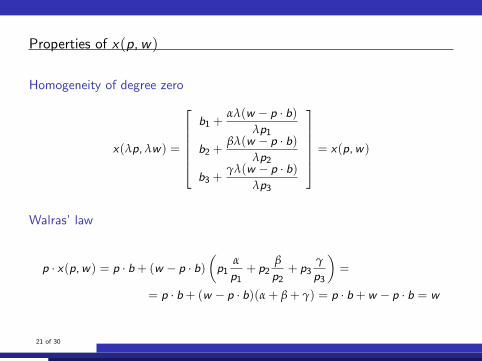
Properties of x(p,w)

Homogeneity of degree zero

x(λp, λw) =

b1 +

αλ(w − p · b)λp1

b2 +βλ(w − p · b)

λp2

b3 +γλ(w − p · b)

λp3

= x(p,w)

Walras’ law

p · x(p,w) = p · b+ (w − p · b)(p1

α

p1+ p2

β

p2+ p3

γ

p3

)=

= p · b+ (w − p · b)(α + β + γ) = p · b+w − p · b = w

21 of 30

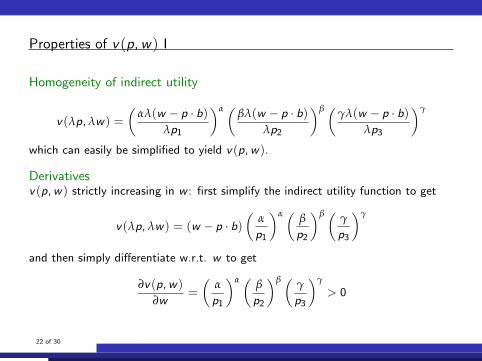
Properties of v(p,w) I

Homogeneity of indirect utility

v(λp, λw) =

(αλ(w − p · b)

λp1

)α ( βλ(w − p · b)λp2

)β (γλ(w − p · b)λp3

)γ

which can easily be simplified to yield v(p,w).

Derivativesv(p,w) strictly increasing in w : first simplify the indirect utility function to get

v(λp, λw) = (w − p · b)(

α

p1

)α ( β

p2

)β ( γ

p3

)γ

and then simply differentiate w.r.t. w to get

∂v(p,w)

∂w=

(α

p1

)α ( β

p2

)β ( γ

p3

)γ

> 0

22 of 30

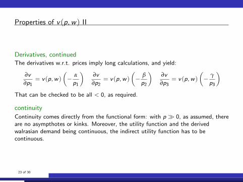
Properties of v(p,w) II

Derivatives, continuedThe derivatives w.r.t. prices imply long calculations, and yield:

∂v

∂p1= v(p,w)

(− α

p1

)∂v

∂p2= v(p,w)

(− β

p2

)∂v

∂p3= v(p,w)

(− γ

p3

)That can be checked to be all < 0, as required.

continuity

Continuity comes directly from the functional form: with p � 0, as assumed, thereare no asympthotes or kinks. Moreover, the utility function and the derivedwalrasian demand being continuous, the indirect utility function has to becontinuous.

23 of 30

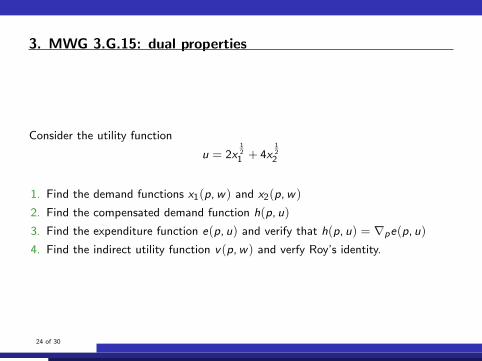
3. MWG 3.G.15: dual properties

Consider the utility function

u = 2x12

1 + 4x12

2

1. Find the demand functions x1(p,w) and x2(p,w)

2. Find the compensated demand function h(p, u)

3. Find the expenditure function e(p, u) and verify that h(p, u) = ∇pe(p, u)

4. Find the indirect utility function v(p,w) and verfy Roy’s identity.

24 of 30

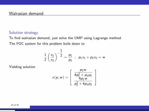
Walrasian demand

Solution strategy

To find walrasian demand, just solve the UMP using Lagrange method.

The FOC system for this problem boils down to

1

2

(x1

x2

)−1

2 =p1

p2; p1x1 + p2x2 = w

Yielding solution

x(p,w) =

p2w

4p21 + p1p24p1w

p22 + 4p1p2

25 of 30

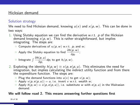
Hicksian demand

Solution strategy

We need to find Hicksian demand, knowing u(x) and x(p,w). This can be done intwo ways:

1. Using Slutsky equation we can find the derivative w.r.t. p of the Hicksiandemand knowing x(p,w). This is rather straightforward, but impliesintegrating. The steps are:◦ Compute derivatives of xl (p,w ) w.r.t. pl and w ;

◦ Apply the Slutsky equation to find∂h(p,w )

∂pl;

◦ Integrate∫ ∂h(p, u)

∂pldpl to get hl (p,w ).

2. Exploting the identity h(p,w) ≡ x(p, e(p, u). This eliminates the need forintegration, but implies calculating the indirect utility function and from therethe expenditure function. The steps are:◦ Plug the demand functions into u(x) to get v (p,w );◦ Apply v (p, e(p, u)) = u, i.e. invert v w.r.t. wealth w ;◦ Apply h(p,w ) ≡ x(p, e(p, u)), i.e. substitute w with e(p, u) in the Walrasian

demand.

We will follow road 2. This means answering further questions first

26 of 30

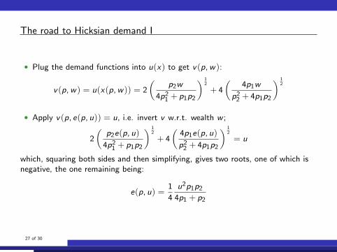
The road to Hicksian demand I

• Plug the demand functions into u(x) to get v(p,w):

v(p,w) = u(x(p,w)) = 2

(p2w

4p21 + p1p2

) 12

+ 4

(4p1w

p22 + 4p1p2

) 12

• Apply v(p, e(p, u)) = u, i.e. invert v w.r.t. wealth w ;

2

(p2e(p, u)

4p21 + p1p2

) 12

+ 4

(4p1e(p, u)

p22 + 4p1p2

) 12

= u

which, squaring both sides and then simplifying, gives two roots, one of which isnegative, the one remaining being:

e(p, u) =1

4

u2p1p2

4p1 + p2

27 of 30

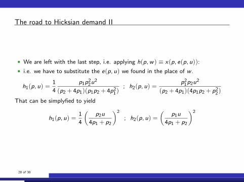
The road to Hicksian demand II

• We are left with the last step, i.e. applying h(p,w) ≡ x(p, e(p, u)):

• i.e. we have to substitute the e(p, u) we found in the place of w .

h1(p, u) =1

4

p1p22u

2

(p2 + 4p1)(p1p2 + 4p21)

; h2(p, u) =p2

1p2u2

(p2 + 4p1)(4p1p2 + p22)

That can be simplyfied to yield

h1(p, u) =1

4

(p2u

4p1 + p2

)2

; h2(p, u) =

(p1u

4p1 + p2

)2

28 of 30

Expenditure function

Solution strategy

Again, we have two ways of finding the expenditure function:

1. Retrieve v(p,w) from x(p,w) and u(x), then invert it w.r.t. w to get e(p, u);

2. Retrieve e(p, u) directly from h(p, u) plugging it in the objective function p · x .

• As for us, we used road 1 and already worked out e(p, u) in the road towardsHicksian demand, so no need to do it here.

• You can easily check by yourself that h(p, u) = ∇pe(p, u)

29 of 30

Roy’s identity

Solution strategy

We can find v(p,w) fromn either v(p,w) = u(x(p,w)) or inverting e(p, u) w.r.t.u; then, we just need to apply Roy’s identity right hand side and check if the resultis the same as the x(p,w) we calculated beforehand. We have to check if thisholds:

xl (p,w) = − ∂v(p,w)

∂pl

(∂v(p,w)

∂w

)−1

, for l = 1, 2

As for us, we already found v(p,w). It’s easy again to apply the formula and findthat Roy’s Identity holds

30 of 30