Embed Size (px)
Citation preview
Problem 2. Evolutionary Strategies.
Victor Montiel Argaiz
January 31, 2012
Contents
1 Introduction 2
2 Description of the Evolutionary Strategy 4
3 Code Structure and implementation 53.1 General Structure . . . . . . . . . . . . . . . . . . . . . . . . . . . . . . . . . . . . . . . . . 53.2 Code Flow . . . . . . . . . . . . . . . . . . . . . . . . . . . . . . . . . . . . . . . . . . . . . 6
4 Results 64.1 Sphere Model . . . . . . . . . . . . . . . . . . . . . . . . . . . . . . . . . . . . . . . . . . . 6
4.1.1 (µ, λ) strategy with uncorrelated one-step mutation . . . . . . . . . . . . . . . . . 64.1.2 (µ, λ) strategy with uncorrelated n-step mutation . . . . . . . . . . . . . . . . . . . 84.1.3 (µ+ λ) strategy with uncorrelated one-step mutation . . . . . . . . . . . . . . . . 94.1.4 (µ+ λ) strategy with uncorrelated n-step mutation . . . . . . . . . . . . . . . . . . 104.1.5 Conclusions for the sphere model . . . . . . . . . . . . . . . . . . . . . . . . . . . . 10
4.2 De Jong’s test function number 5 . . . . . . . . . . . . . . . . . . . . . . . . . . . . . . . . 144.2.1 (µ, λ) strategy with uncorrelated one-step mutation . . . . . . . . . . . . . . . . . 154.2.2 (µ, λ) strategy with uncorrelated n-step mutation . . . . . . . . . . . . . . . . . . . 164.2.3 (µ+ λ) strategy with uncorrelated one-step mutation . . . . . . . . . . . . . . . . 174.2.4 (µ+ λ) strategy with uncorrelated n-step mutation . . . . . . . . . . . . . . . . . . 194.2.5 Conclusions for the De Jong model . . . . . . . . . . . . . . . . . . . . . . . . . . . 19
4.3 Schwefel’s function . . . . . . . . . . . . . . . . . . . . . . . . . . . . . . . . . . . . . . . . 234.3.1 (µ, λ) strategy with uncorrelated one-step mutation . . . . . . . . . . . . . . . . . 234.3.2 (µ, λ) strategy with uncorrelated n-step mutation . . . . . . . . . . . . . . . . . . . 264.3.3 (µ+ λ) strategy with uncorrelated one-step mutation . . . . . . . . . . . . . . . . 284.3.4 (µ+ λ) strategy with uncorrelated n-step mutation . . . . . . . . . . . . . . . . . . 304.3.5 Conclusions for the Schwefel’s function . . . . . . . . . . . . . . . . . . . . . . . . . 31
5 Summary and Conclusions 32
6 Appendix 33
A Program Compilation 33
B Program Execution 33
1
1 Introduction
In this problem set we explore the capabilities of Evolutionary Strategies, a technique within the Evo-lutionary Computation family used for function optimization. The technique is used against three testfunction used to measure the effectiveness of optimization functions [3].
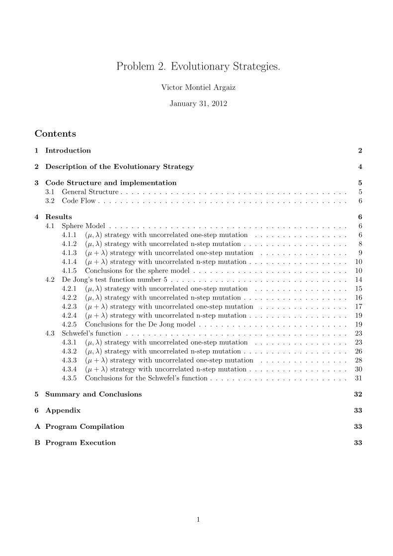
The first function is the Sphere model, described in equation (1). The function, that for this problemhas been ranged within the hypercube [−10, 10]n, is smooth (C∞), symmetrical with respect to any ofthe coordinate axis, and has a sole local minimum located at x∗ = 〈0, 0, . . . 0〉 and with value f(x∗) = 0.0.With these properties, the search process is straightforward, and even simple search algorithms couldfind it. A plot of the Sphere model can be found in figure (1).
f(x) =n∑i=1
x2i (1)
Figure 1: Sphere model. Picture from MatLab GEATbx
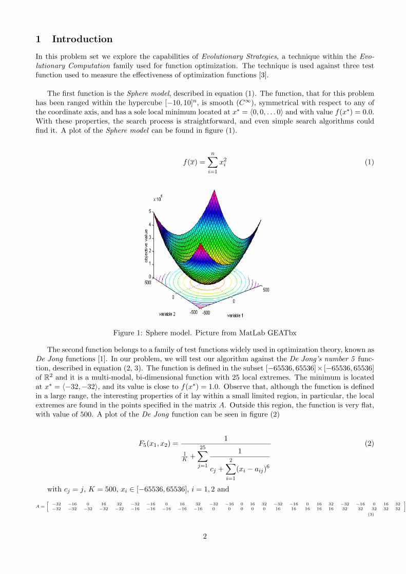
The second function belongs to a family of test functions widely used in optimization theory, known asDe Jong functions [1]. In our problem, we will test our algorithm against the De Jong’s number 5 func-tion, described in equation (2, 3). The function is defined in the subset [−65536, 65536]× [−65536, 65536]of R2 and it is a multi-modal, bi-dimensional function with 25 local extremes. The minimum is locatedat x∗ = 〈−32,−32〉, and its value is close to f(x∗) = 1.0. Observe that, although the function is definedin a large range, the interesting properties of it lay within a small limited region, in particular, the localextremes are found in the points specified in the matrix A. Outside this region, the function is very flat,with value of 500. A plot of the De Jong function can be seen in figure (2)
F5(x1, x2) =1
1K +
25∑j=1
1
cj +2∑i=1
(xi − aij)6
(2)
with cj = j, K = 500, xi ∈ [−65536, 65536], i = 1, 2 and
A =
[−32 −16 0 16 32 −32 −16 0 16 32 −32 −16 0 16 32 −32 −16 0 16 32 −32 −16 0 16 32−32 −32 −32 −32 −32 −16 −16 −16 −16 −16 0 0 0 0 0 16 16 16 16 16 32 32 32 32 32
](3)
2
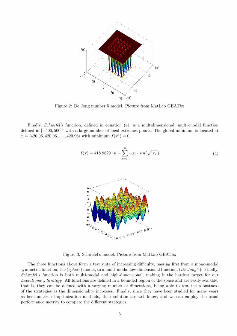
Figure 2: De Jong number 5 model. Picture from MatLab GEATbx
Finally, Schwefel’s function, defined in equation (4), is a multidimensional, multi-modal functiondefined in [−500, 500]n with a large number of local extremes points. The global minimum is located atx = 〈420.96, 420.96, . . . , 420.96〉 with minimum f(x∗) = 0.
f(x) = 418.9829 · n+n∑i=1
−xi · sin(√|xi|) (4)
Figure 3: Schwefel’s model. Picture from MatLab GEATbx
The three functions above form a test suite of increasing difficulty, passing first from a mono-modalsymmetric function, the (sphere) model, to a multi-modal low-dimensional function, (De Jong’s). Finally,Schwefel’s function is both multi-modal and high-dimensional, making it the hardest target for ourEvolutionary Strategy. All functions are defined in a bounded region of the space and are easily scalable,that is, they can be defined with a varying number of dimensions, being able to test the robustnessof the strategies as the dimensionality increases. Finally, since they have been studied for many yearsas benchmarks of optimization methods, their solution are well-know, and we can employ the usualperformance metrics to compare the different strategies.
3
2 Description of the Evolutionary Strategy
For real-valued functions of type Rn 7→ R, the natural genotype representation for the problem is an-dimensional vector of real values, being n de dimension of the function to be minimized. Additionally,the genotype is extended to include the control parameters of the algorithm, as we shall see, dependingon the mutation scheme we use.
Mutation and recombinator operators for this representation are similar to those used in genetic algo-rithms techniques. For the mutator operator, we use random increments in each of the alleles, accordingto a normal distribution whose standard deviation varies with the evolutionary process. Amongst thethree most common mutations, uncorrelated one-step, uncorrelated n-step and correlated, we have evalu-ated the performance of the first two methods.
In the former one, explained in equation (5), the search (mutation) is done by adding randomincrements located in an hyper-sphere, i.e., the distance from the original point is ‘equal’ (in probabilityterms) in all dimensions, since we are using the same σ for all axis.
σ′ = max(σ · eτN(0,1), ε0)
x′i = xi + σ′Ni(0, 1)(5)
The second mutation, explained in formula (6), accepts different scale factors, σi, for each of thedimensions, creating hyper-ellipses around the original point, thus, allowing larger variations for someaxes than for others.
σ′i = max(σi · eτ′N(0,1)+τNi(0,1), ε0)
x′i = xi + σ′iNi(0, 1)(6)
Observe that, dealing with bounded functions defined in a finite subset of the Rn space, we have todefine somehow what to do with the individuals that, after the mutation process, are located outsidethe region where the function is defined. The first approach was to limit the individual to the range ofdefinition of the function, so, those individual exceeding that range for any the dimension were forced tobe at the boundary. This approach did not result in good results, specially for the De Jong’s function,as we will see, where most of the individual ended up located in the boundary of the function because ofthe special properties of the test model. To overcome this problem, we defined a method to ‘create’ validindividuals, i.e., within the range of definition of the function, after a mutation. The idea is to apply theconcept of modular arithmetic to each dimension, and so, when for one of the dimensions i, the point xiexceed the range of definition of the function by δ, this point is transformed in x′i = xi,0 + δ as if therange were circular, being xi,0 the lower bound in the range of definition for the dimension i.
Finally, for the recombinator operator, we distinguish between the object part, encoding the point inthe space, and the strategy parameters part, encoding the parameters which control the mutation process.For the first one we use discrete recombination, choosing randomly the value of one of the parents, and,for the second one we use intermediary recombination, averaging the values of the parents’ parameterto create the offspring parameter. This way, diversity within the solution space is assured, allowingvery different combinations of values in the search process, and at the same time, the averaging in theparameter genes performs a more cautious adaptation.
4
3 Code Structure and implementation
3.1 General Structure
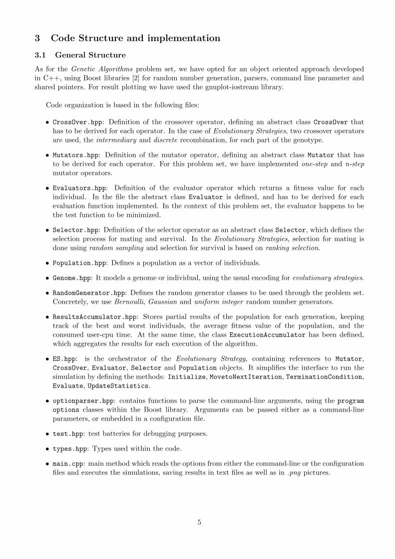
As for the Genetic Algorithms problem set, we have opted for an object oriented approach developedin C++, using Boost libraries [2] for random number generation, parsers, command line parameter andshared pointers. For result plotting we have used the gnuplot-iostream library.
Code organization is based in the following files:
• CrossOver.hpp: Definition of the crossover operator, defining an abstract class CrossOver thathas to be derived for each operator. In the case of Evolutionary Strategies, two crossover operatorsare used, the intermediary and discrete recombination, for each part of the genotype.
• Mutators.hpp: Definition of the mutator operator, defining an abstract class Mutator that hasto be derived for each operator. For this problem set, we have implemented one-step and n-stepmutator operators.
• Evaluators.hpp: Definition of the evaluator operator which returns a fitness value for eachindividual. In the file the abstract class Evaluator is defined, and has to be derived for eachevaluation function implemented. In the context of this problem set, the evaluator happens to bethe test function to be minimized.
• Selector.hpp: Definition of the selector operator as an abstract class Selector, which defines theselection process for mating and survival. In the Evolutionary Strategies, selection for mating isdone using random sampling and selection for survival is based on ranking selection.
• Population.hpp: Defines a population as a vector of individuals.
• Genome.hpp: It models a genome or individual, using the usual encoding for evolutionary strategies.
• RandomGenerator.hpp: Defines the random generator classes to be used through the problem set.Concretely, we use Bernoulli, Gaussian and uniform integer random number generators.
• ResultsAccumulator.hpp: Stores partial results of the population for each generation, keepingtrack of the best and worst individuals, the average fitness value of the population, and theconsumed user-cpu time. At the same time, the class ExecutionAccumulator has been defined,which aggregates the results for each execution of the algorithm.
• ES.hpp: is the orchestrator of the Evolutionary Strategy, containing references to Mutator,CrossOver, Evaluator, Selector and Population objects. It simplifies the interface to run thesimulation by defining the methods: Initialize, MovetoNextIteration, TerminationCondition,Evaluate, UpdateStatistics.
• optionparser.hpp: contains functions to parse the command-line arguments, using the program
options classes within the Boost library. Arguments can be passed either as a command-lineparameters, or embedded in a configuration file.
• test.hpp: test batteries for debugging purposes.
• types.hpp: Types used within the code.
• main.cpp: main method which reads the options from either the command-line or the configurationfiles and executes the simulations, saving results in text files as well as in .png pictures.
5

3.2 Code Flow
The execution flow of the program can be summarized, according to the code in the main method, asfollows:
• Step 1: Parsing of the command-line arguments with the parameters defining the simulation to berun.
• Step 2: Creation of the operators to be used by the Evolutionary Strategy. This includes themutation, recombination, evaluation and selection operators. Creation of the population object.
• Step 3: Creation of the ES object instance, passing as arguments the operators to be used in thestrategy, and creation of the ResultAccumulator objects, to keep track of the partial results.
• Step 4: For each execution to be run, initialization of the evolutionary strategy, invoking theInitialize method on the ES object.
• Step 5: Repetition of the evolutionary process until the termination condition, i.e., maximumnumber of generation, is achieved. The instructions repeated in the loop are, by this order, selectionof parents, recombination of parents, creation of a new population with off-springs and eventuallyoriginal parents, depending on the scheme of the strategy. Then, mutation of the individuals of thepopulation, evaluation of the resulting individuals and selection of survivors is performed.
• Step 6: The loop above is repeated for each generation, for each execution of the problem, until allinstances have been run. Then, by constructing an ExecutionAccumulator object, we summarizethe results of all of the executions of the strategy plotting charts and printing partial results to.csv text files.
4 Results
4.1 Sphere Model
As we discussed in the introduction, the sphere model is the simplest function studied in this problem set.Its smooth behavior, the existence of a unique extreme point along with its symmetry makes the functionan easy target even for simple optimization methods. Being Evolutionary Strategies robust optimizationmethods even for the hardest test function, we expect that the experiments in this section are easilyresolved, even for a large number of dimensions.
Results for this section have been made by executing the program using the following parametersfiles: question2a.cfg, question2b.cfg, question2c.cfg, question2d.cfg.
4.1.1 (µ, λ) strategy with uncorrelated one-step mutation
In figure (4) we have plotted the estimation of the minimum value for the test function, using the simplestone-step mutation, achieving pretty good and accurate results for the optimization. All of the 30 simu-lations we have run draw similar results, achieving, with minimum error (of 10e−7 order), the minimumof the function, located at x∗ = 〈0, . . . , 0〉, and with value fsphere(x
∗) = 0. In the same figure (4) we havesummarized the statistics of the best-fitted individual for the 30 executions. The range of the results,difference between worst and best cases, is really small, and the standard deviation of the population lieswithin the 10−8 order of magnitude.
In figure (5) we have plotted the evolution of the solution for one of the executions using logarithmicaxis to really appreciate the speed of convergence. As we can see, convergence to the minimum is reallyfast, and within a few generations we reach function values close to the minimum up to the order of theminimum error, 10e−7 in this case. As we will see later, this convergence error is closely related to the
6
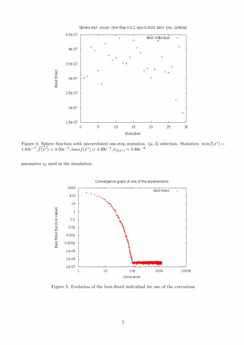
Figure 4: Sphere function with uncorrelated one-step mutation. (µ, λ) selection. Statistics: minf(x∗) =1.83e−7, f(x∗) = 3.50e−7,maxf(x∗) = 4.39e−7, σf(x∗) = 5.89e−8
parameter ε0 used in the simulation.
Figure 5: Evolution of the best-fitted individual for one of the executions
7
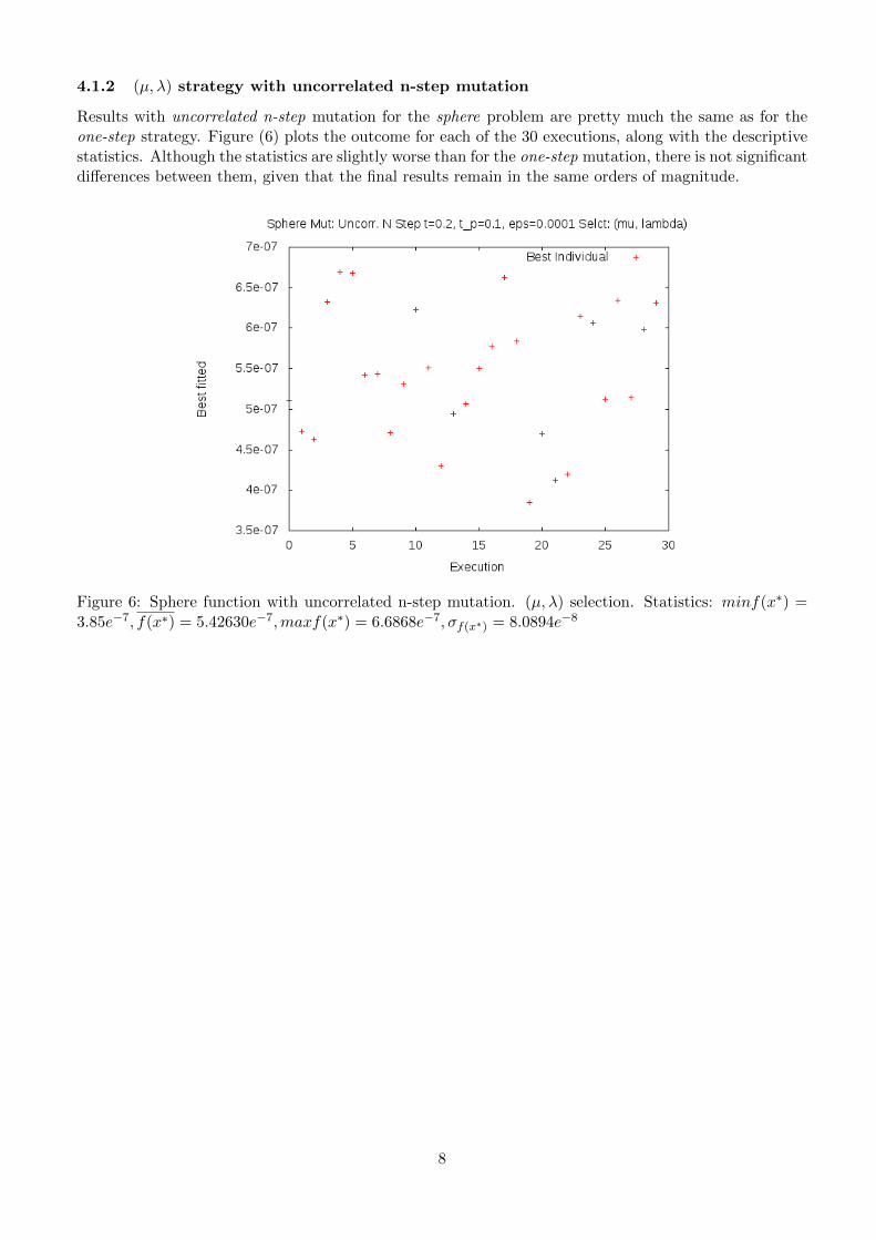
4.1.2 (µ, λ) strategy with uncorrelated n-step mutation
Results with uncorrelated n-step mutation for the sphere problem are pretty much the same as for theone-step strategy. Figure (6) plots the outcome for each of the 30 executions, along with the descriptivestatistics. Although the statistics are slightly worse than for the one-step mutation, there is not significantdifferences between them, given that the final results remain in the same orders of magnitude.
Figure 6: Sphere function with uncorrelated n-step mutation. (µ, λ) selection. Statistics: minf(x∗) =3.85e−7, f(x∗) = 5.42630e−7,maxf(x∗) = 6.6868e−7, σf(x∗) = 8.0894e−8
8
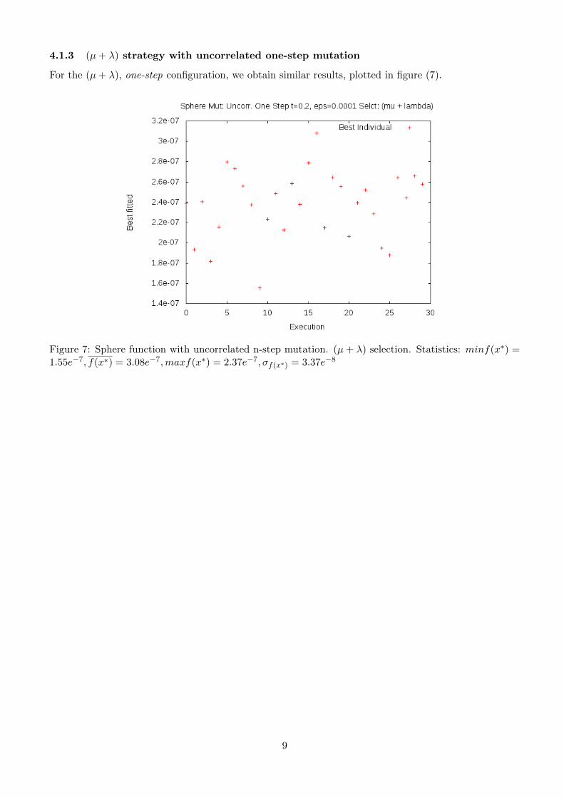
4.1.3 (µ+ λ) strategy with uncorrelated one-step mutation
For the (µ+ λ), one-step configuration, we obtain similar results, plotted in figure (7).
Figure 7: Sphere function with uncorrelated n-step mutation. (µ+ λ) selection. Statistics: minf(x∗) =1.55e−7, f(x∗) = 3.08e−7,maxf(x∗) = 2.37e−7, σf(x∗) = 3.37e−8
9
4.1.4 (µ+ λ) strategy with uncorrelated n-step mutation
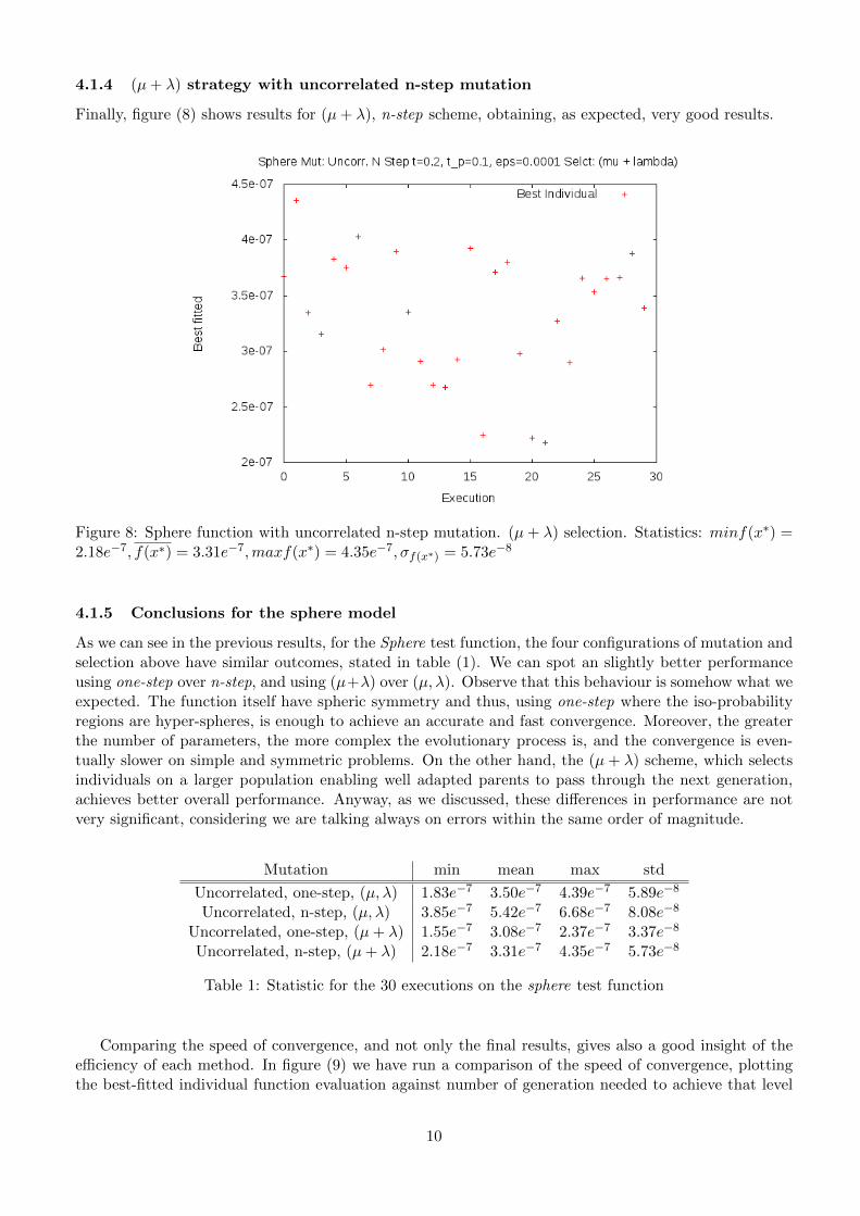
Finally, figure (8) shows results for (µ+ λ), n-step scheme, obtaining, as expected, very good results.
Figure 8: Sphere function with uncorrelated n-step mutation. (µ+ λ) selection. Statistics: minf(x∗) =2.18e−7, f(x∗) = 3.31e−7,maxf(x∗) = 4.35e−7, σf(x∗) = 5.73e−8
4.1.5 Conclusions for the sphere model
As we can see in the previous results, for the Sphere test function, the four configurations of mutation andselection above have similar outcomes, stated in table (1). We can spot an slightly better performanceusing one-step over n-step, and using (µ+λ) over (µ, λ). Observe that this behaviour is somehow what weexpected. The function itself have spheric symmetry and thus, using one-step where the iso-probabilityregions are hyper-spheres, is enough to achieve an accurate and fast convergence. Moreover, the greaterthe number of parameters, the more complex the evolutionary process is, and the convergence is even-tually slower on simple and symmetric problems. On the other hand, the (µ+ λ) scheme, which selectsindividuals on a larger population enabling well adapted parents to pass through the next generation,achieves better overall performance. Anyway, as we discussed, these differences in performance are notvery significant, considering we are talking always on errors within the same order of magnitude.
Mutation min mean max std
Uncorrelated, one-step, (µ, λ) 1.83e−7 3.50e−7 4.39e−7 5.89e−8
Uncorrelated, n-step, (µ, λ) 3.85e−7 5.42e−7 6.68e−7 8.08e−8
Uncorrelated, one-step, (µ+ λ) 1.55e−7 3.08e−7 2.37e−7 3.37e−8
Uncorrelated, n-step, (µ+ λ) 2.18e−7 3.31e−7 4.35e−7 5.73e−8
Table 1: Statistic for the 30 executions on the sphere test function
Comparing the speed of convergence, and not only the final results, gives also a good insight of theefficiency of each method. In figure (9) we have run a comparison of the speed of convergence, plottingthe best-fitted individual function evaluation against number of generation needed to achieve that level
10
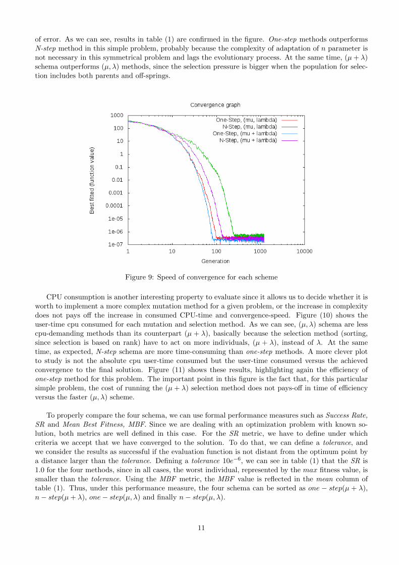
of error. As we can see, results in table (1) are confirmed in the figure. One-step methods outperformsN-step method in this simple problem, probably because the complexity of adaptation of n parameter isnot necessary in this symmetrical problem and lags the evolutionary process. At the same time, (µ+ λ)schema outperforms (µ, λ) methods, since the selection pressure is bigger when the population for selec-tion includes both parents and off-springs.
Figure 9: Speed of convergence for each scheme
CPU consumption is another interesting property to evaluate since it allows us to decide whether it isworth to implement a more complex mutation method for a given problem, or the increase in complexitydoes not pays off the increase in consumed CPU-time and convergence-speed. Figure (10) shows theuser-time cpu consumed for each mutation and selection method. As we can see, (µ, λ) schema are lesscpu-demanding methods than its counterpart (µ + λ), basically because the selection method (sorting,since selection is based on rank) have to act on more individuals, (µ + λ), instead of λ. At the sametime, as expected, N-step schema are more time-consuming than one-step methods. A more clever plotto study is not the absolute cpu user-time consumed but the user-time consumed versus the achievedconvergence to the final solution. Figure (11) shows these results, highlighting again the efficiency ofone-step method for this problem. The important point in this figure is the fact that, for this particularsimple problem, the cost of running the (µ + λ) selection method does not pays-off in time of efficiencyversus the faster (µ, λ) scheme.
To properly compare the four schema, we can use formal performance measures such as Success Rate,SR and Mean Best Fitness, MBF. Since we are dealing with an optimization problem with known so-lution, both metrics are well defined in this case. For the SR metric, we have to define under whichcriteria we accept that we have converged to the solution. To do that, we can define a tolerance, andwe consider the results as successful if the evaluation function is not distant from the optimum point bya distance larger than the tolerance. Defining a tolerance 10e−6, we can see in table (1) that the SR is1.0 for the four methods, since in all cases, the worst individual, represented by the max fitness value, issmaller than the tolerance. Using the MBF metric, the MBF value is reflected in the mean column oftable (1). Thus, under this performance measure, the four schema can be sorted as one − step(µ + λ),n− step(µ+ λ), one− step(µ, λ) and finally n− step(µ, λ).
11
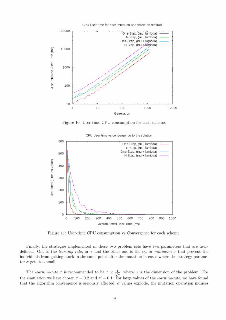
Figure 10: User-time CPU consumption for each scheme.
Figure 11: User-time CPU consumption vs Convergence for each scheme.
Finally, the strategies implemented in these two problem sets have two parameters that are user-defined. One is the learning rate, or τ and the other one is the ε0, or minimum σ that prevent theindividuals from getting stuck in the same point after the mutation in cases where the strategy parame-ter σ gets too small.
The learning-rate τ is recommended to be τ ∝ 1√n
, where n is the dimension of the problem. For
the simulation we have chosen τ = 0.2 and τ ′ = 0.1. For large values of the learning-rate, we have foundthat the algorithm convergence is seriously affected, σ values explode, the mutation operation induces
12

big changes in the individuals and the population after a single mutation is so different that evolutionaryprocess have difficulties in retain the best individuals. For smaller values of the learning-rate, the conver-gence is still guaranteed, although the speed of convergence is reduced, being necessary more than 1200generations in order to achieve reasonable results.
As for the ε0 parameter, we have used 0.0001 for this problem. For unimodal function, as the one inthis section, it is preferred to be small, since convergence to the unique extreme point is easier, we donot need a big variety in the population to find the path to this point. By assuring a small ε0 we areguarantying a higher accuracy in the final solution, since the paths leading to the minimum point arerather easy to find. By increase the ε0 value, the algorithm still advance to the surrounding points of theoptimum value, but, however, once it reaches the surrounding points, due to σ values cannot fall belowε0, the solution is always jumping amongst points around the minimum, instead of converging with moreaccuracy to the minimum value. Thus, we have observed that the accuracy of the solution in this problemis directly proportional to the value of the ε0. For ε0 values smaller than two decimal places, 10e−2, weachieve solutions accurate up to three decimal places, and for orders of magnitude of four decimal places,we have achieved solutions accurate up to seven decimal places.
13

4.2 De Jong’s test function number 5
The characteristics of De Jong’s function represent an arduous task for the designed Evolutionary Strate-gies. The fact of having up to 25 extreme points requires more diversity in the strategy to avoid beingstuck in local minima. But the difficult problem to overcome is the shape of the function, defined in[−65536, 65536] × [−65536, 65536], where in most of the space the function has a flat value of 500 andonly on a tiny region of the function domain, specifically, the subset defined in [−32, 32]× [−32, 32], theinteresting extreme points are concentrated. Observe that, the region of the space where the ‘real action’takes places represent a small portion of the domain. Consider a bi-dimensional uniform probability dis-tribution, the probability of a point to lay on the interesting region where extreme points are concentratedis 64·64
131072·131072 ≈ 2.38·10−7. Observe that with a configuration of µ = 30, λ = 200, generations = 1200 weevaluate, at each execution, 7.2 ·106 individuals. Thus, the proportion between the number of individualsevaluated and the probability for an individual being in the ‘interesting region’ is quite scarce for thealgorithm to perform in good conditions, specially when the region outside the [−32, 32]×[−32, 32] subsetis flat. That is the reason why using (µ+λ) schema, where the selection process is performed on a largerbase of individuals, will cast better results. Increasing the number of off-springs at each generation willhave the same effect, and will improve considerably the performance of the strategy.
Aware of this difficulty, we run the simulations suggested in the problem set. Since in most cases wehave not achieved a reasonable level of convergence to the solution, specially on the (µ, λ), we have runthe same simulation with a larger number of off-springs at each generation, λ = 800. As above-mentioned,by increasing the number of individuals at each selection, we increase the probability that some of theindividuals is near the ‘interesting region’ where the extreme points are located, thus, improving consid-erably the convergence of the algorithm.
An interesting feature that we have been forced to implement to tackle with this test function is thefunctionality of limiting the individuals to the range of definition of the function. As described in theprevious section, the mutation process can lead to individuals which are outside the boundary of defini-tion of the function. In the special case of the De Jong’s test function, since most of the function havea flat 500 value, many individuals were projected outside the [−65536, 65536] × [−65536, 65536] rangeafter mutation. Using the ‘modular arithmetic’ idea explained above we have successfully improved theperformance of the evolutionary strategy, by relocating the individuals projected outside the domain ofdefinition of the function inside the same domain.
Finally, by reducing the range of definition of the function to a smaller subset, the results would havebeen considerably better, not having been necessary to increase the population size, λ, to achieve SRmetrics close to 1.0.
Results for this section have been made by executing the program using the following parametersfiles: question6a.cfg, question6b.cfg, question6c.cfg, question6d.cfg and question6a 800.cfg,question6b 800.cfg, question6c 800.cfg, question6d 800.cfg
14
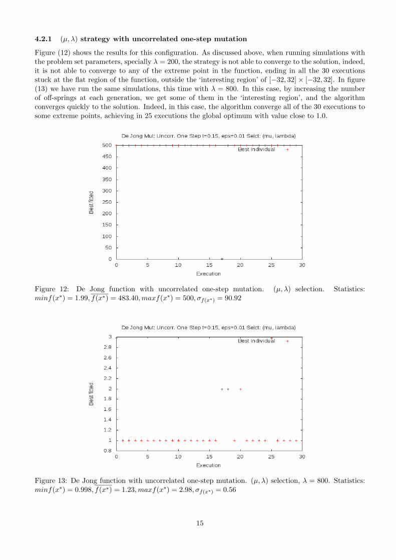
4.2.1 (µ, λ) strategy with uncorrelated one-step mutation
Figure (12) shows the results for this configuration. As discussed above, when running simulations withthe problem set parameters, specially λ = 200, the strategy is not able to converge to the solution, indeed,it is not able to converge to any of the extreme point in the function, ending in all the 30 executionsstuck at the flat region of the function, outside the ‘interesting region’ of [−32, 32]× [−32, 32]. In figure(13) we have run the same simulations, this time with λ = 800. In this case, by increasing the numberof off-springs at each generation, we get some of them in the ‘interesting region’, and the algorithmconverges quickly to the solution. Indeed, in this case, the algorithm converge all of the 30 executions tosome extreme points, achieving in 25 executions the global optimum with value close to 1.0.
Figure 12: De Jong function with uncorrelated one-step mutation. (µ, λ) selection. Statistics:minf(x∗) = 1.99, f(x∗) = 483.40,maxf(x∗) = 500, σf(x∗) = 90.92
Figure 13: De Jong function with uncorrelated one-step mutation. (µ, λ) selection, λ = 800. Statistics:minf(x∗) = 0.998, f(x∗) = 1.23,maxf(x∗) = 2.98, σf(x∗) = 0.56
15
4.2.2 (µ, λ) strategy with uncorrelated n-step mutation
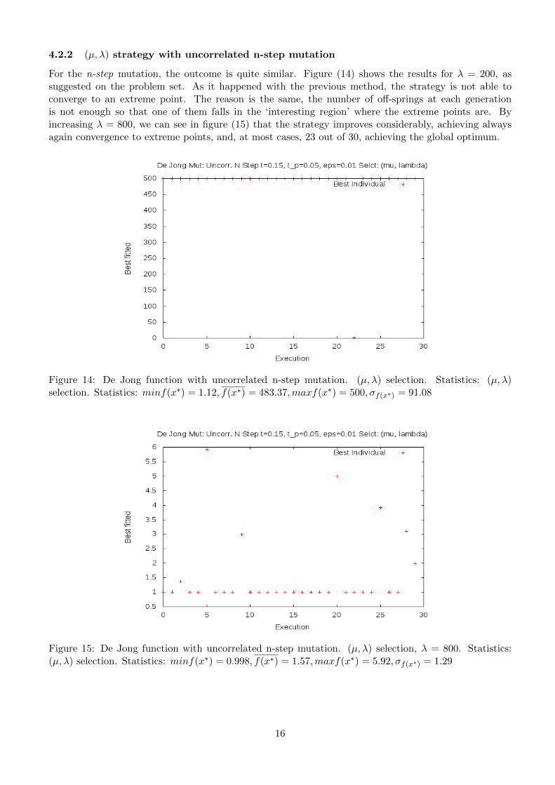
For the n-step mutation, the outcome is quite similar. Figure (14) shows the results for λ = 200, assuggested on the problem set. As it happened with the previous method, the strategy is not able toconverge to an extreme point. The reason is the same, the number of off-springs at each generationis not enough so that one of them falls in the ‘interesting region’ where the extreme points are. Byincreasing λ = 800, we can see in figure (15) that the strategy improves considerably, achieving alwaysagain convergence to extreme points, and, at most cases, 23 out of 30, achieving the global optimum.
Figure 14: De Jong function with uncorrelated n-step mutation. (µ, λ) selection. Statistics: (µ, λ)selection. Statistics: minf(x∗) = 1.12, f(x∗) = 483.37,maxf(x∗) = 500, σf(x∗) = 91.08
Figure 15: De Jong function with uncorrelated n-step mutation. (µ, λ) selection, λ = 800. Statistics:(µ, λ) selection. Statistics: minf(x∗) = 0.998, f(x∗) = 1.57,maxf(x∗) = 5.92, σf(x∗) = 1.29
16
4.2.3 (µ+ λ) strategy with uncorrelated one-step mutation
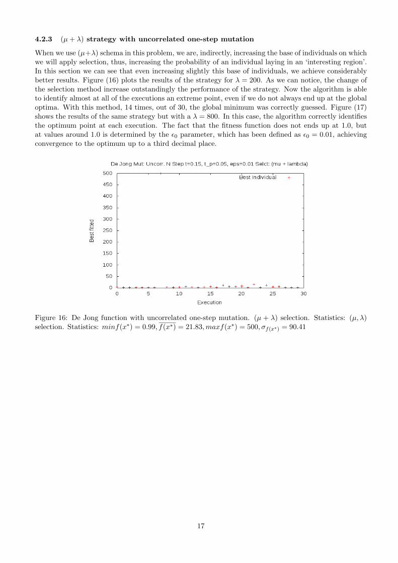
When we use (µ+λ) schema in this problem, we are, indirectly, increasing the base of individuals on whichwe will apply selection, thus, increasing the probability of an individual laying in an ‘interesting region’.In this section we can see that even increasing slightly this base of individuals, we achieve considerablybetter results. Figure (16) plots the results of the strategy for λ = 200. As we can notice, the change ofthe selection method increase outstandingly the performance of the strategy. Now the algorithm is ableto identify almost at all of the executions an extreme point, even if we do not always end up at the globaloptima. With this method, 14 times, out of 30, the global minimum was correctly guessed. Figure (17)shows the results of the same strategy but with a λ = 800. In this case, the algorithm correctly identifiesthe optimum point at each execution. The fact that the fitness function does not ends up at 1.0, butat values around 1.0 is determined by the ε0 parameter, which has been defined as ε0 = 0.01, achievingconvergence to the optimum up to a third decimal place.
Figure 16: De Jong function with uncorrelated one-step mutation. (µ + λ) selection. Statistics: (µ, λ)selection. Statistics: minf(x∗) = 0.99, f(x∗) = 21.83,maxf(x∗) = 500, σf(x∗) = 90.41
17
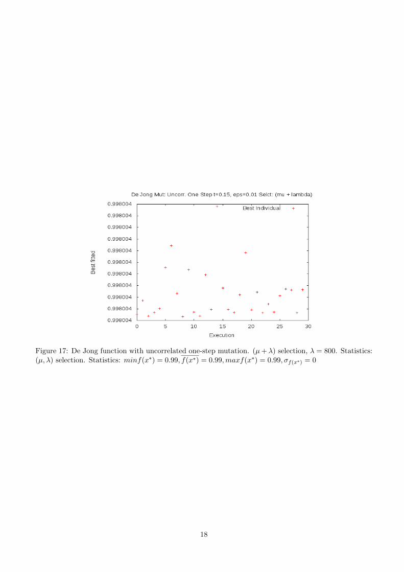
Figure 17: De Jong function with uncorrelated one-step mutation. (µ+ λ) selection, λ = 800. Statistics:(µ, λ) selection. Statistics: minf(x∗) = 0.99, f(x∗) = 0.99,maxf(x∗) = 0.99, σf(x∗) = 0
18
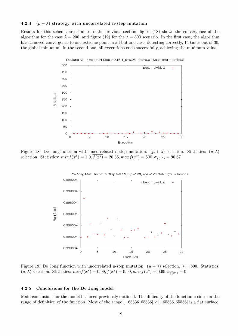
4.2.4 (µ+ λ) strategy with uncorrelated n-step mutation
Results for this schema are similar to the previous section, figure (18) shows the convergence of thealgorithm for the case λ = 200, and figure (19) for the λ = 800 scenario. In the first case, the algorithmhas achieved convergence to one extreme point in all but one case, detecting correctly, 14 times out of 30,the global minimum. In the second one, all executions ends successfully, achieving the minimum value.
Figure 18: De Jong function with uncorrelated n-step mutation. (µ + λ) selection. Statistics: (µ, λ)selection. Statistics: minf(x∗) = 1.0, f(x∗) = 20.35,maxf(x∗) = 500, σf(x∗) = 90.67
Figure 19: De Jong function with uncorrelated n-step mutation. (µ + λ) selection, λ = 800. Statistics:(µ, λ) selection. Statistics: minf(x∗) = 0.99, f(x∗) = 0.99,maxf(x∗) = 0.99, σf(x∗) = 0
4.2.5 Conclusions for the De Jong model
Main conclusions for the model has been previously outlined. The difficulty of the function resides on therange of definition of the function. Most of the range [−65536, 65536]× [−65536, 65536] is a flat surface,
19
λ = 200 λ = 800Mutation min mean max std min mean max std
Uncorrelated, one-step, (µ, λ) 1.99 483.40 500 90.92 0.998 1.23 2.98 0.56Uncorrelated, n-step, (µ, λ) 1.12 483.37 500 91.08 0.998 1.57 5.92 1.29
Uncorrelated, one-step, (µ+ λ) 0.99 21.83 500 90.41 0.99 0.99 0.99 0.00Uncorrelated, n-step, (µ+ λ) 0.99 20.35 500 90.67 0.99 0.99 0.99 0.00
Table 2: Statistic for the 30 executions on the De Jong test function
and extreme points are located in a region limited to [−32, 32] × [−32, 32]. A key aspect to bypass thisissue is to increase the number of individuals taking part in the selection process at each generation,either by choosing (µ + λ) schema or by increase the λ parameter. Both strategies have been provedsuccessful to work around this problem, preferring increasing λ for a maximum accuracy at the expenseof an important increase in CPU-time. A more detailed study would reveal the optimum λ to achieveconvergence without wasting too much CPU-time.
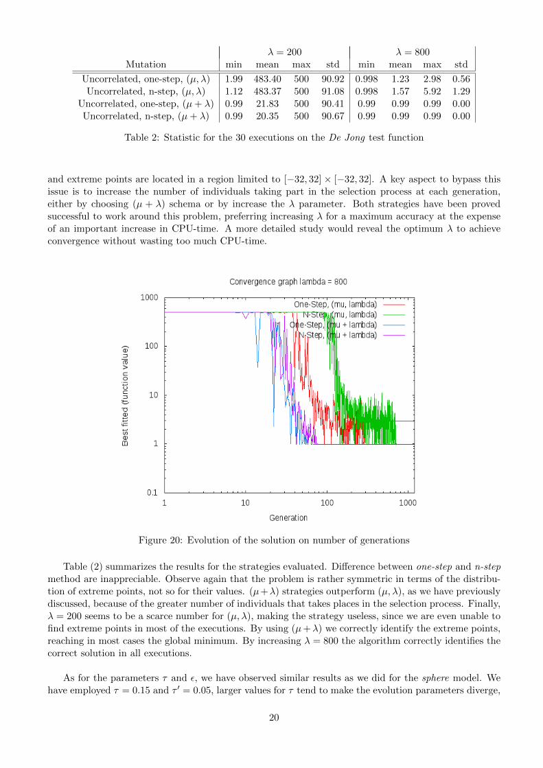
Figure 20: Evolution of the solution on number of generations
Table (2) summarizes the results for the strategies evaluated. Difference between one-step and n-stepmethod are inappreciable. Observe again that the problem is rather symmetric in terms of the distribu-tion of extreme points, not so for their values. (µ+λ) strategies outperform (µ, λ), as we have previouslydiscussed, because of the greater number of individuals that takes places in the selection process. Finally,λ = 200 seems to be a scarce number for (µ, λ), making the strategy useless, since we are even unable tofind extreme points in most of the executions. By using (µ+λ) we correctly identify the extreme points,reaching in most cases the global minimum. By increasing λ = 800 the algorithm correctly identifies thecorrect solution in all executions.
As for the parameters τ and ε, we have observed similar results as we did for the sphere model. Wehave employed τ = 0.15 and τ ′ = 0.05, larger values for τ tend to make the evolution parameters diverge,
20
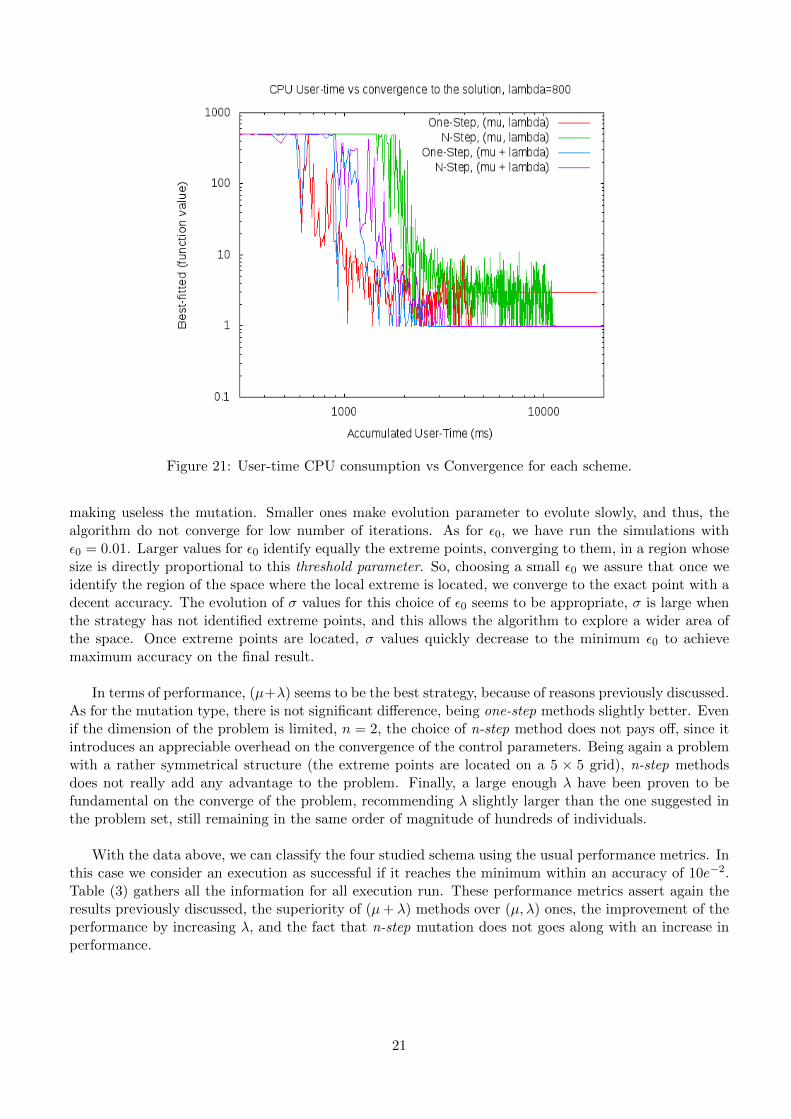
Figure 21: User-time CPU consumption vs Convergence for each scheme.
making useless the mutation. Smaller ones make evolution parameter to evolute slowly, and thus, thealgorithm do not converge for low number of iterations. As for ε0, we have run the simulations withε0 = 0.01. Larger values for ε0 identify equally the extreme points, converging to them, in a region whosesize is directly proportional to this threshold parameter. So, choosing a small ε0 we assure that once weidentify the region of the space where the local extreme is located, we converge to the exact point with adecent accuracy. The evolution of σ values for this choice of ε0 seems to be appropriate, σ is large whenthe strategy has not identified extreme points, and this allows the algorithm to explore a wider area ofthe space. Once extreme points are located, σ values quickly decrease to the minimum ε0 to achievemaximum accuracy on the final result.
In terms of performance, (µ+λ) seems to be the best strategy, because of reasons previously discussed.As for the mutation type, there is not significant difference, being one-step methods slightly better. Evenif the dimension of the problem is limited, n = 2, the choice of n-step method does not pays off, since itintroduces an appreciable overhead on the convergence of the control parameters. Being again a problemwith a rather symmetrical structure (the extreme points are located on a 5 × 5 grid), n-step methodsdoes not really add any advantage to the problem. Finally, a large enough λ have been proven to befundamental on the converge of the problem, recommending λ slightly larger than the one suggested inthe problem set, still remaining in the same order of magnitude of hundreds of individuals.
With the data above, we can classify the four studied schema using the usual performance metrics. Inthis case we consider an execution as successful if it reaches the minimum within an accuracy of 10e−2.Table (3) gathers all the information for all execution run. These performance metrics assert again theresults previously discussed, the superiority of (µ+ λ) methods over (µ, λ) ones, the improvement of theperformance by increasing λ, and the fact that n-step mutation does not goes along with an increase inperformance.
21
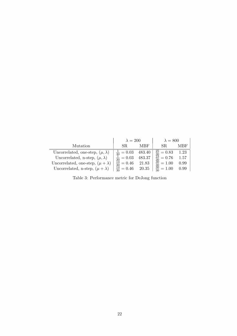
λ = 200 λ = 800Mutation SR MBF SR MBF
Uncorrelated, one-step, (µ, λ) 130 = 0.03 483.40 25
30 = 0.83 1.23Uncorrelated, n-step, (µ, λ) 1
30 = 0.03 483.37 2330 = 0.76 1.57
Uncorrelated, one-step, (µ+ λ) 1430 = 0.46 21.83 30
30 = 1.00 0.99Uncorrelated, n-step, (µ+ λ) 14
30 = 0.46 20.35 3030 = 1.00 0.99
Table 3: Performance metric for DeJong function
22
4.3 Schwefel’s function
Schwefel’s test function have some properties that make it a harder target for evolutionary strategy.The minimum of the function is located in a point of the space where all the components have the value420.9687. The relevant characteristics that make the function troublesome for evolutionary strategies are,firstly, that it is defined in a space of d = 20 dimensions and secondly, it is a multi-modal function, witha large number of extreme points. The first property makes more difficult the job for the ES, since theevolutionary process for a large number of parameters is cumbersome, making convergence slower. Thesecond one can make that the ES gets stuck in some local extreme points. Concretely, for the Schwefel’s,we have observed that the ES developed got stuck at points x where most of the components xi ≈ 420.97and some of them where different from the optimum value for that coordinate. These points happen tobe local extreme points where, once the algorithm converge, it is difficult to get it out of there.
Since for the suggested parameters to solve this problem set we have not achieved in most cases thecorrect solution, we have explored some other different configurations to fine tune our ES. In concrete, wehave run executions with the suggested parameters, λ = 200, other with a reduced dimensions of d = 10,and other with a larger population of λ = 800.
As a general result, the problems with d = 10 have been correctly solved, indicating that the highdimensionality of the function is responsible for the complexity of the optimization process. Executionsfor λ = 800 have performed better, since they have been able to get the ES out of the local extremepoints where the strategies with smaller population get stuck.
Results for this section have been made by executing the program using the following parame-ters files: question7a.cfg, question7a-dim-10.cfg, question7a-lambda-800.cfg,question7b.cfg,question7b-dim-10.cfg, question7b-lambda-800.cfg, question7c.cfg, question7c-dim-10.cfg,question7c-lambda-800.cfg, question7d.cfg, question7d-dim-10.cfg, question7d-lambda-800.cfg.
4.3.1 (µ, λ) strategy with uncorrelated one-step mutation
In figure (22) we can appreciate the results for the suggested configuration of the problem. As we canobserve, convergence to the minimum is achieved only in 3 out of 30 executions. By increasing λ = 800,we can notice in figure (23) that results improve slightly, but still they are not good enough to use thisstrategy. In this case solution is achieved 6 out of 30 executions, the remaining ones ending up stuckin non-optimal extreme points. Finally, by reducing the dimensionality of the problem to d = 10, thesuccess rate improves up to 18 out of 30, thus, observing the added complexity of the problem when thenumber of dimension is large.
23
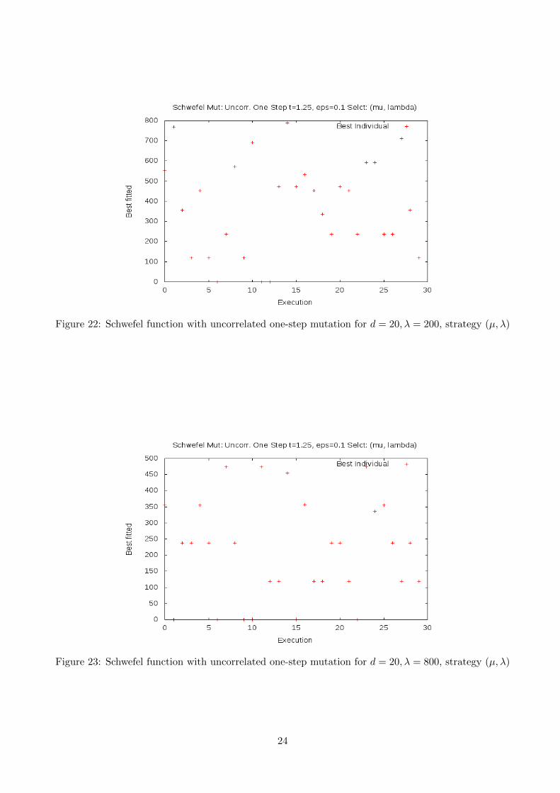
Figure 22: Schwefel function with uncorrelated one-step mutation for d = 20, λ = 200, strategy (µ, λ)
Figure 23: Schwefel function with uncorrelated one-step mutation for d = 20, λ = 800, strategy (µ, λ)
24
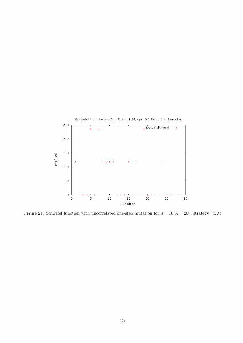
Figure 24: Schwefel function with uncorrelated one-step mutation for d = 10, λ = 200, strategy (µ, λ)
25
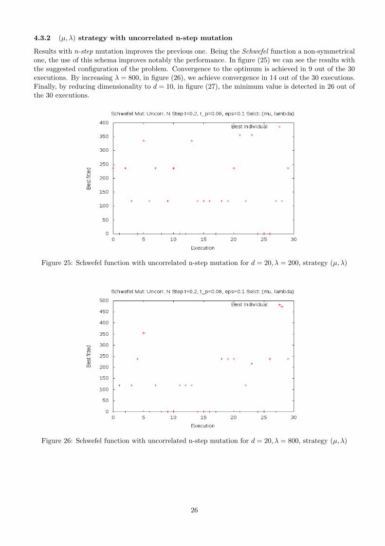
4.3.2 (µ, λ) strategy with uncorrelated n-step mutation
Results with n-step mutation improves the previous one. Being the Schwefel function a non-symmetricalone, the use of this schema improves notably the performance. In figure (25) we can see the results withthe suggested configuration of the problem. Convergence to the optimum is achieved in 9 out of the 30executions. By increasing λ = 800, in figure (26), we achieve convergence in 14 out of the 30 executions.Finally, by reducing dimensionality to d = 10, in figure (27), the minimum value is detected in 26 out ofthe 30 executions.
Figure 25: Schwefel function with uncorrelated n-step mutation for d = 20, λ = 200, strategy (µ, λ)
Figure 26: Schwefel function with uncorrelated n-step mutation for d = 20, λ = 800, strategy (µ, λ)
26
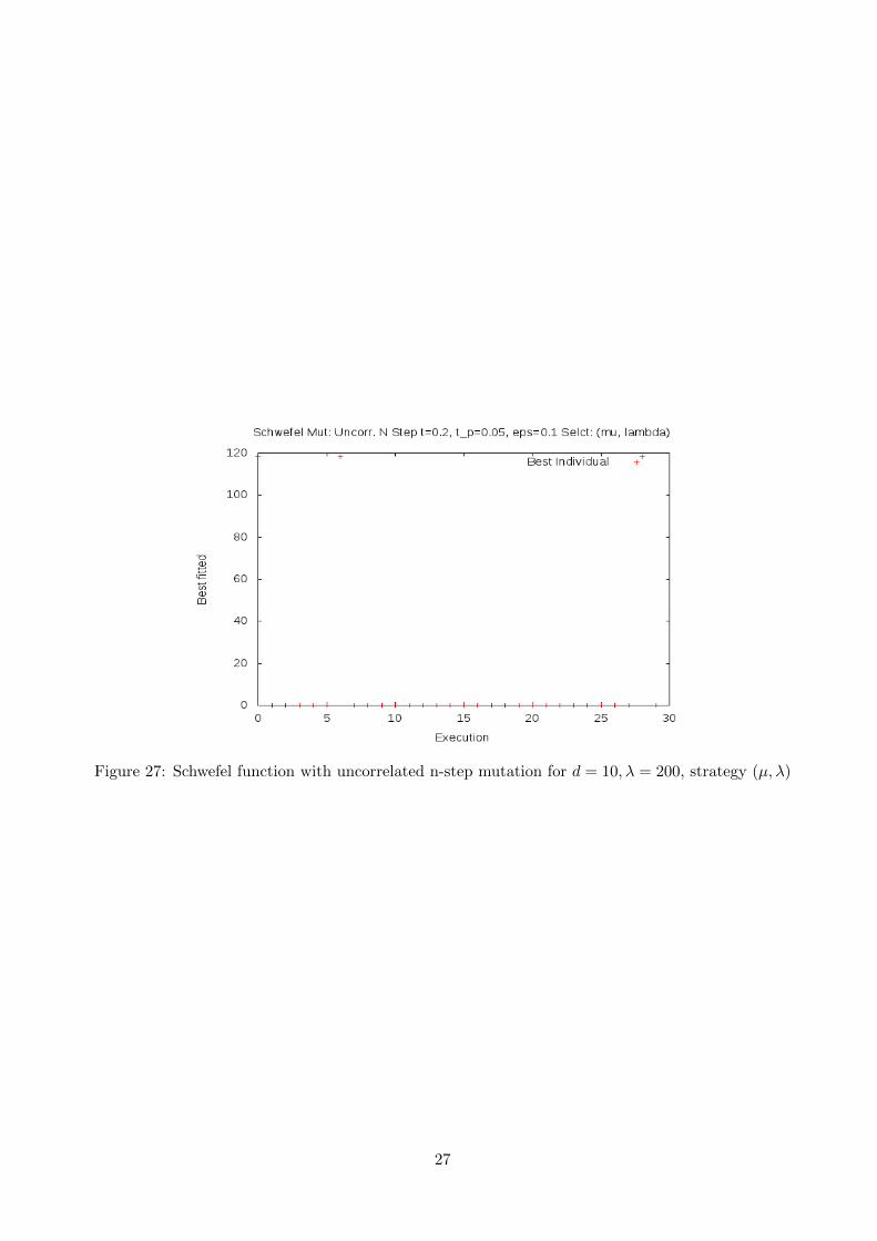
Figure 27: Schwefel function with uncorrelated n-step mutation for d = 10, λ = 200, strategy (µ, λ)
27
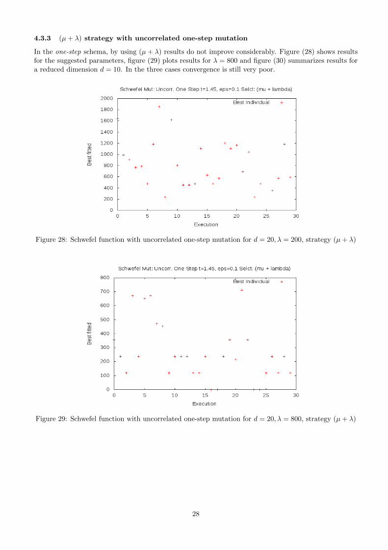
4.3.3 (µ+ λ) strategy with uncorrelated one-step mutation
In the one-step schema, by using (µ+ λ) results do not improve considerably. Figure (28) shows resultsfor the suggested parameters, figure (29) plots results for λ = 800 and figure (30) summarizes results fora reduced dimension d = 10. In the three cases convergence is still very poor.
Figure 28: Schwefel function with uncorrelated one-step mutation for d = 20, λ = 200, strategy (µ+ λ)
Figure 29: Schwefel function with uncorrelated one-step mutation for d = 20, λ = 800, strategy (µ+ λ)
28
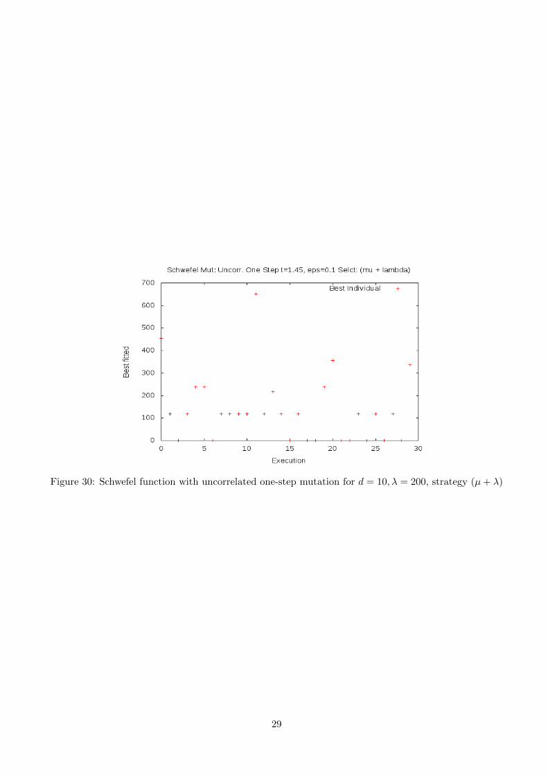
Figure 30: Schwefel function with uncorrelated one-step mutation for d = 10, λ = 200, strategy (µ+ λ)
29
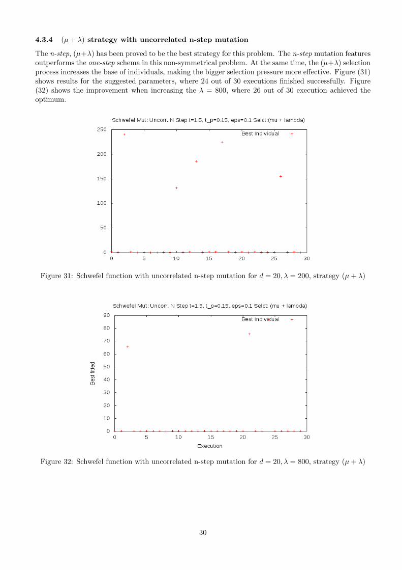
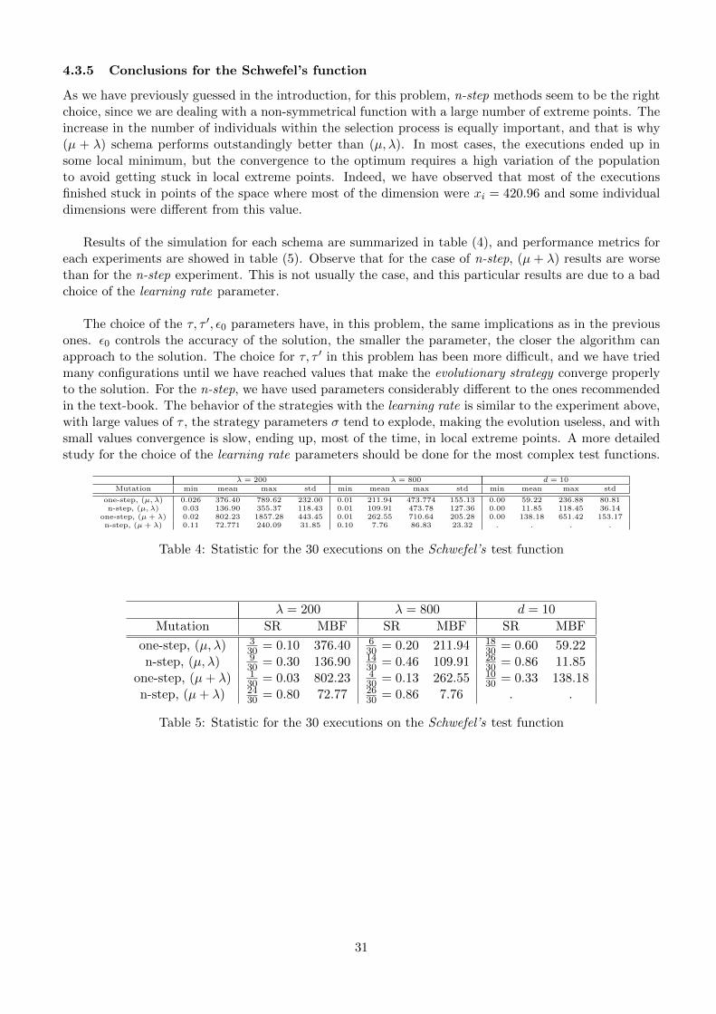
4.3.4 (µ+ λ) strategy with uncorrelated n-step mutation
The n-step, (µ+λ) has been proved to be the best strategy for this problem. The n-step mutation featuresoutperforms the one-step schema in this non-symmetrical problem. At the same time, the (µ+λ) selectionprocess increases the base of individuals, making the bigger selection pressure more effective. Figure (31)shows results for the suggested parameters, where 24 out of 30 executions finished successfully. Figure(32) shows the improvement when increasing the λ = 800, where 26 out of 30 execution achieved theoptimum.
Figure 31: Schwefel function with uncorrelated n-step mutation for d = 20, λ = 200, strategy (µ+ λ)
Figure 32: Schwefel function with uncorrelated n-step mutation for d = 20, λ = 800, strategy (µ+ λ)
30
4.3.5 Conclusions for the Schwefel’s function
As we have previously guessed in the introduction, for this problem, n-step methods seem to be the rightchoice, since we are dealing with a non-symmetrical function with a large number of extreme points. Theincrease in the number of individuals within the selection process is equally important, and that is why(µ + λ) schema performs outstandingly better than (µ, λ). In most cases, the executions ended up insome local minimum, but the convergence to the optimum requires a high variation of the populationto avoid getting stuck in local extreme points. Indeed, we have observed that most of the executionsfinished stuck in points of the space where most of the dimension were xi = 420.96 and some individualdimensions were different from this value.
Results of the simulation for each schema are summarized in table (4), and performance metrics foreach experiments are showed in table (5). Observe that for the case of n-step, (µ+ λ) results are worsethan for the n-step experiment. This is not usually the case, and this particular results are due to a badchoice of the learning rate parameter.
The choice of the τ, τ ′, ε0 parameters have, in this problem, the same implications as in the previousones. ε0 controls the accuracy of the solution, the smaller the parameter, the closer the algorithm canapproach to the solution. The choice for τ, τ ′ in this problem has been more difficult, and we have triedmany configurations until we have reached values that make the evolutionary strategy converge properlyto the solution. For the n-step, we have used parameters considerably different to the ones recommendedin the text-book. The behavior of the strategies with the learning rate is similar to the experiment above,with large values of τ , the strategy parameters σ tend to explode, making the evolution useless, and withsmall values convergence is slow, ending up, most of the time, in local extreme points. A more detailedstudy for the choice of the learning rate parameters should be done for the most complex test functions.
λ = 200 λ = 800 d = 10Mutation min mean max std min mean max std min mean max std
one-step, (µ, λ) 0.026 376.40 789.62 232.00 0.01 211.94 473.774 155.13 0.00 59.22 236.88 80.81n-step, (µ, λ) 0.03 136.90 355.37 118.43 0.01 109.91 473.78 127.36 0.00 11.85 118.45 36.14
one-step, (µ + λ) 0.02 802.23 1857.28 443.45 0.01 262.55 710.64 205.28 0.00 138.18 651.42 153.17n-step, (µ + λ) 0.11 72.771 240.09 31.85 0.10 7.76 86.83 23.32 . . . .
Table 4: Statistic for the 30 executions on the Schwefel’s test function
λ = 200 λ = 800 d = 10
Mutation SR MBF SR MBF SR MBF
one-step, (µ, λ) 330 = 0.10 376.40 6
30 = 0.20 211.94 1830 = 0.60 59.22
n-step, (µ, λ) 930 = 0.30 136.90 14
30 = 0.46 109.91 2630 = 0.86 11.85
one-step, (µ+ λ) 130 = 0.03 802.23 4
30 = 0.13 262.55 1030 = 0.33 138.18
n-step, (µ+ λ) 2430 = 0.80 72.77 26
30 = 0.86 7.76 . .
Table 5: Statistic for the 30 executions on the Schwefel’s test function
31
5 Summary and Conclusions
We have tested three function of increased difficulty: mono-modal symmetrical function (sphere),multi-modal, low-dimensional, quasi-symmetrical function (De Jongs) and highly-multi-modal, highly-dimensional asymmetrical function (Schwefel). N-step methods have been proved to be preferred forhighly-dimensional and asymmetric functions, where the cost of evolving n control parameters pays offthe improvement in performance. (µ + λ) methods have been shown superior to (µ, λ), since selectionis made on a larger base of individuals. However, depending on the values of µ, λ parameter, and thedifficulty of the test function, the increase in cpu user-time consumed does not justify the increase inperformance, specially for easy problems as the sphere model.
Parameters such as learning rate, τ, τ ′ have to be carefully chosen, specially in difficult problems. Theconvergence and stability of the evolutionary strategy depends greatly on them. Finally, ε0 parameterscan be used to set a desired accuracy when converging to the optimal value.
Correlated mutation methods have been not tested on this problem set. As we have seen, in mostcases, the increase in the number of control parameters carries more complexity for the evolutionaryprocess, making harder or slower, at sometimes, the convergence. In the case of correlated methods, thenumber of control parameters to evolve explodes with the number of dimensions, needing to evolve nσ-parameters and n(n−1)
2 α parameters, making the method awkward even for low dimensional problems.
In all of the three problems we have obtained good levels of SR metrics, with a sample of 30 executions.For the first two test function, optimal configuration of selection and mutation method have achievedoutstanding SR = 1.0 rating. For the more difficult third problem, we have obtained SR = 0.86. Therewould be, however, large room to improve the SR in this case, just by increasing the population size.
32

6 Appendix
A Program Compilation
Program building process has be done using the standard make gnu tool. To compile and link theprogram just invoke the make command on the root directory. The binaries will be found either underthe bin/debug or bin/release directories, depending on the dbg flag specified at config.mk file. Tolink the program and generate the binary, we need the Boost Libraries properly installed in our system.The libraries.mk file contains the list of libraries that we need for the linking process.
B Program Execution
The program ES.bin is invoked from the command line, passing all required parameters needed to theexecution of the algorithm. For a comprehensive list of parameters, we can invoke:
victor@kokomero:~/ES.bin --help
Allowed options:
--conf_file arg Path to the configuration file. If omitted,
arguments are read from command line
--epsilon arg Minimum value for the std
--test_function arg Test function: sphere, dejong, schwefel
--search_space arg value of the search space, if x, search will be
limited to [-x, x] for each dimension
--dimension arg Dimension parameter n, for Sphere and Schwefel test
function
--mutation arg Mutator operator, one of: onestep (uncorrelated
one-step), multistep (uncorrelated n-step),
correlated (correlated)
--tau arg Tau parameter for mutation
--tau_p arg Tau prima parameter for n-step mutation
--selection arg Selection operator, one of: replacement (mu,
lambda) or competition (mu + lambda)
--mu arg (=30) Number of individuals in the population
--lambda arg (=200) Number of offsprings created at each generation
--generations arg (=1200) Number of generations for the termination condition
--executions arg (=10) Number of independent executions
--test Run mutation and crossover tests for debuggin
purposes
--help print out help message
All configuration parameters can be specified in a .cfg file, as the one below, question7a.cfg:
mutation=onestep
tau=1.25
tau_p=0.25
epsilon=0.1
dimension=20
search_space=500
test_function=schwefel
selection=replacement
mu=30
lambda=200
generations=1200
executions=30
33
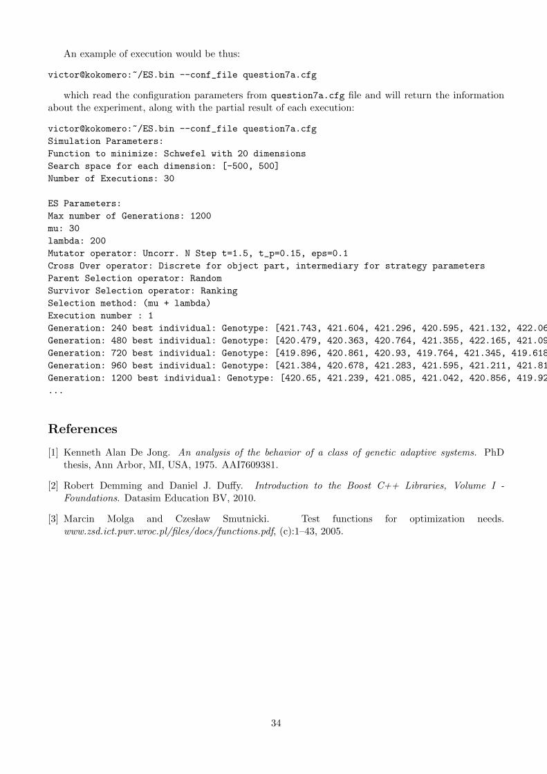
An example of execution would be thus:
victor@kokomero:~/ES.bin --conf_file question7a.cfg
which read the configuration parameters from question7a.cfg file and will return the informationabout the experiment, along with the partial result of each execution:
victor@kokomero:~/ES.bin --conf_file question7a.cfg
Simulation Parameters:
Function to minimize: Schwefel with 20 dimensions
Search space for each dimension: [-500, 500]
Number of Executions: 30
ES Parameters:
Max number of Generations: 1200
mu: 30
lambda: 200
Mutator operator: Uncorr. N Step t=1.5, t_p=0.15, eps=0.1
Cross Over operator: Discrete for object part, intermediary for strategy parameters
Parent Selection operator: Random
Survivor Selection operator: Ranking
Selection method: (mu + lambda)
Execution number : 1
Generation: 240 best individual: Genotype: [421.743, 421.604, 421.296, 420.595, 421.132, 422.06, 420.798, 421.24, 421.01, 421.448, 420.505, 421.226, 422.372, 420.255, 420.511, 420.735, 421.123, 421.688, 421.05, 419.822] Parameters: [0.253394, 0.1, 0.1, 0.1, 0.253251, 0.481849, 0.1, 0.650344, 0.128395, 0.148951, 0.424667, 0.1, 3.12457, 0.1, 0.32588, 0.25887, 1.40835, 0.1, 0.159001, 0.1] Evaluation: 0.970424
Generation: 480 best individual: Genotype: [420.479, 420.363, 420.764, 421.355, 422.165, 421.097, 421.073, 422.661, 421.376, 420.438, 421.236, 420.775, 419.976, 419.613, 420.899, 421.434, 420.85, 421.461, 421.151, 420.343] Parameters: [0.217094, 0.1, 0.1, 0.642167, 0.150633, 6.79873, 0.1, 0.445065, 0.66669, 0.1, 0.202898, 0.1, 1.57066, 0.1, 0.212328, 0.1, 0.1, 0.260615, 0.1, 0.602719] Evaluation: 1.18676
Generation: 720 best individual: Genotype: [419.896, 420.861, 420.93, 419.764, 421.345, 419.618, 420.837, 420.318, 420.421, 421.324, 421.22, 421.659, 421.502, 420.702, 421.912, 421.803, 419.986, 420.544, 420.862, 420.702] Parameters: [0.123191, 0.1, 0.1, 0.271035, 0.15667, 0.1, 1.3523, 0.387428, 0.1, 0.1, 0.127385, 0.160261, 0.1, 1.08275, 0.1, 0.30193, 0.744522, 0.1, 0.503309, 1.01854] Evaluation: 1.15591
Generation: 960 best individual: Genotype: [421.384, 420.678, 421.283, 421.595, 421.211, 421.815, 420.589, 421.628, 420.413, 420.734, 419.83, 420.137, 420.623, 422.941, 420.952, 420.64, 421.163, 420.358, 421.214, 419.983] Parameters: [0.528732, 0.297997, 0.128335, 0.134524, 0.110813, 0.308237, 0.123991, 1.12307, 0.1, 0.284337, 0.19775, 1.36144, 0.145004, 0.169273, 0.259961, 1.74799, 1.51859, 0.185328, 0.1, 0.276092] Evaluation: 1.26397
Generation: 1200 best individual: Genotype: [420.65, 421.239, 421.085, 421.042, 420.856, 419.925, 420.819, 421.384, 421.338, 421.679, 421.038, 420.671, 421.614, 422.007, 421.897, 420.763, 422.439, 420.881, 420.693, 420.49] Parameters: [0.609772, 0.281603, 1.04236, 0.1, 0.261246, 0.1, 0.301839, 0.13052, 0.1, 0.479103, 2.04525, 0.21966, 0.1, 0.409315, 0.246084, 0.1, 0.509332, 0.131262, 0.399745, 0.1] Evaluation: 0.89597
...
References
[1] Kenneth Alan De Jong. An analysis of the behavior of a class of genetic adaptive systems. PhDthesis, Ann Arbor, MI, USA, 1975. AAI7609381.
[2] Robert Demming and Daniel J. Duffy. Introduction to the Boost C++ Libraries, Volume I -Foundations. Datasim Education BV, 2010.
[3] Marcin Molga and Czes law Smutnicki. Test functions for optimization needs.www.zsd.ict.pwr.wroc.pl/files/docs/functions.pdf, (c):1–43, 2005.
34