PROBABILITY AND VARIANCE-BASED … deterministic optimization, ... usually stochastic programming algorithms or ... hensive study of the use of the combination of genetic algorithms

V International Conference on Computational Methods for Coupled Problems in Science and EngineeringCOUPLED PROBLEMS 2013

S. Idelsohn, M. Papadrakakis and B. Schrefler (Eds)

PROBABILITY AND VARIANCE-BASED STOCHASTICDESIGN OPTIMIZATION OF A RADIAL COMPRESSOR

CONCERNING FLUID-STRUCTURE INTERACTION

DIRK ROOS∗, KEVIN CREMANNS & TIM JASPER

Institute of Modelling and High-Performance ComputingNiederrhein University of Applied SciencesReinarzstr. 49, D-47805 Krefeld, Germany

e-mail: dirk.roos[@]hs-niederrhein.de

Key words: robust design optimization, robustness evaluation, reliability analysis,fluid-structure interaction, surrogate models, adaptive design of experiment, impor-tance sampling, directional sampling

Abstract. Since the engineering of turbo machines began the improvement of spe-cific physical behaviour, especially the efficiency, has been one of the key issues.However, improvement of the efficiency of a turbo engine, is hard to archive using aconventional deterministic optimization, since the geometry is not perfect and manyother parameters vary in the real approach.

In contrast, stochastic design optimization is a methodology that enables thesolving of optimization problems which model the effects of uncertainty in manufac-turing, design configuration and environment, in which robustness and reliability areexplicit optimization goals. Therein, a coupling of stochastic and optimization prob-lems implies high computational efforts, whereby the calculation of the stochasticconstraints represents the main effort. In view of this fact, an industrially relevantalgorithm should satisfy the conditions of precision, robustness and efficiency.

In this paper an efficient approach is presented to assist reducing the number ofdesign evaluations necessary, in particular the number of nonlinear fluid-structureinteraction analyses. In combination with a robust estimation of the safety levelwithin the iteration and a final precise reliability analysis, the method presentedis particularly suitable for solving reliability-based structural design optimizationproblems with ever-changing failure probabilities of the nominal designs.

The applicability for real case applications is demonstrated through the exampleof a radial compressor, with a very high degree of complexity and a large number ofdesign parameters and random variables.

1

Dirk Roos, Kevin Cremanns & Tim Jasper

(nodal variables)

Modelling ofnonlinearities and transient behavior

(mechanical variables)

Finite volume model Finite element model

Geometry model(geometrical variables)

Optimization problem(design parameters)

Stochastic problem(random variables)

(nodal variables)

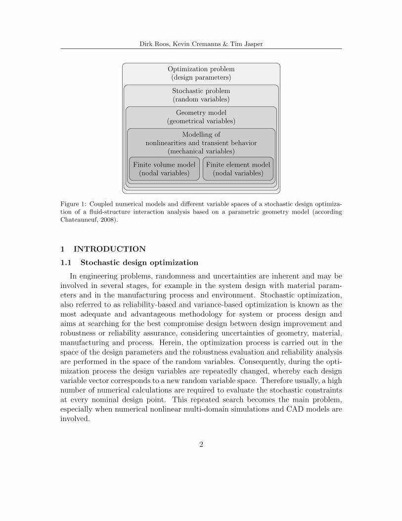
Figure 1: Coupled numerical models and different variable spaces of a stochastic design optimiza-tion of a fluid-structure interaction analysis based on a parametric geometry model (accordingChateauneuf, 2008).

1 INTRODUCTION

1.1 Stochastic design optimization

In engineering problems, randomness and uncertainties are inherent and may beinvolved in several stages, for example in the system design with material param-eters and in the manufacturing process and environment. Stochastic optimization,also referred to as reliability-based and variance-based optimization is known as themost adequate and advantageous methodology for system or process design andaims at searching for the best compromise design between design improvement androbustness or reliability assurance, considering uncertainties of geometry, material,manufacturing and process. Herein, the optimization process is carried out in thespace of the design parameters and the robustness evaluation and reliability analysisare performed in the space of the random variables. Consequently, during the opti-mization process the design variables are repeatedly changed, whereby each designvariable vector corresponds to a new random variable space. Therefore usually, a highnumber of numerical calculations are required to evaluate the stochastic constraintsat every nominal design point. This repeated search becomes the main problem,especially when numerical nonlinear multi-domain simulations and CAD models areinvolved.

2


Unfortunately, in real case applications of the virtual prototyping process, it isnot always possible to reduce the complexity of the physical models to obtain numer-ical models which can be solved quickly. Usually, every single numerical simulationtakes hours or even days. Although progress has been made in identifying numericalmethods to solve stochastic design optimization problems and high performance com-puting, in cases such as those that have several nested numerical models, as shownin Fig. 1, the actual costs of using these methods to explore various model configura-tions for practical applications is too high. Therefore, methods for efficiently solvingstochastic optimization problems based on the introduction of simplifications andspecial formulations for reducing the numerical efforts are required.

1.2 Application to aerodynamic optimization

In comparative studies on the application of the deterministic optimization foraerodynamic optimization (see e.g. Muller-Tows, 2000, Sasaki et al., 2001, Shahpar,2000) usually stochastic programming algorithms or response surface methods (seee.g. Pierret and van den Braembussche, 1999) are used in turbomachinery design, forexample in the development of engine components, such as at Vaidyanathan et al.(2000). In Shyy et al. (2001) a comprehensive overview is represented.

An example of an applied aerodynamic deterministic optimization using a geneticalgorithm is published in Trigg et al. (1997) and the optimized design of transonicprofiles also using genetic algorithms is given in Oyama (2000). Another very compre-hensive study of the use of the combination of genetic algorithms and neural networksfor two-dimensional aerodynamic optimization of profiles is presented in Dennis et al.(1999) combine a genetic algorithm with an gradient-based optimization method.

Furthermore, an increasing application of stochastic analysis on turbo machinery(e.g. at Garzon, 2003, Garzon and Darmofal, 2003, Lange et al., 2010, Parchem andMeissner, 2009) underlines the importance of integrating the uncertainty analysisinto the aerodynamic design process.

2 RELIABILITY-BASED AND VARIANCE-BASED DESIGN OPTI-MIZATION

2.1 Deterministic optimization

Optimization is defined as a procedure to achieve the best outcome of a givenobjective function (sometimes also called cost function) while satisfying certain re-

3


fX1(x1)

f(di) =constd1 = E[X1]

d2

=E

[X2]

d2

f→

min

d0i

di

dIi

d1

f X2(x

2)

∆γ

g(x

j)

=0

u(di, γ) = 0 unsafedomain

P (F)

domainunfeasible

Figure 2: Different solution points dIi or di asresult of a deterministic vs. stochastic designoptimization in the space of given randomlydistributed design parameters.

σy

g(xj, di) = 0

f σe(σ

e)

fσy(σy)

σe

fσIe (σIe)

f σI e(σ

I e)

unsafe domain

P (F)

∆γ

∆σd

σIy = σIeσyσId = σIe

σσy

σy,k

fX(x)

f(di) =const

σd

=σe σσe

f→

min

di

x∗j

xj

dIi

Figure 3: Comparison of the deterministic op-timal point dIi and the solution of a stochasticoptimization di with corresponding most proba-ble failure point x∗j in the space of the randomlydistributed von Mises stress and the yield stress.

strictions. The deterministic optimization problem

f(d1, d2, . . . dnd)→ min

el(d1, d2, . . . dnd) = 0; l = 1, ne

um(d1, d2, . . . dnd ,γ) ≥ 0; m = 1, nu

dli ≤ di ≤ duidi ∈ [dli , dui ] ⊂ Rnd

(1)

is defined by the objective function f : Rnd → R subject to the restrictions, definedas equality and inequality constraints el and um. The variables d1, d2, . . . dnd are theoptimization or design variables and the vector of the partial safety factors γ ensuresthe system or design safety within the constraint equations um, for example defininga safety distance u(d, γ) = yg/γ − yd ≥ 0 between a defined limit state value yg andthe nominal design value yd of a physical response parameter y = f(d). In structuralsafety assessment, a typical constraint for the stress is given as

u(d, γ) = σy,k/γ − σd ≥ 0 (2)

4


ensuring the global safety distance

∆γ = σy,k − σd = σy,k −σy,kγ

= σy,k

(1− 1

γ

)between the defined quantile value σy,k of the yield stress and the nominal designstress σd with the global safety factor γ, as shown in Fig. 3. Whereby, in the realapproach with given uncertainties, σd corresponds to the mean von Mises equivalentstress σe at the current design point.

2.2 Stochastic chance-constrained optimization

Stochastic optimization algorithms use the quantification of uncertainties to pro-duce solutions that optimize the expected performance of a process or design, en-suring the target variances of the model responses and failure probability. So, thedeterministic optimization problem (1) can be enhanced by additional stochasticrestrictions. For example, the expression for system reliability

1− P (F)

P t(F)≥ 0 (3)

ensures that the probability of failure

P (F) = P [X : gk(x) ≤ 0] =

∫nr. . .

∫gk(x)≤0

fX(x)dx (4)

cannot exceed a given target probability P t(F), considering the vector of all randominfluences

X = [X1, X2, ..., Xnr ]T (5)

with the joint probability density function of the random variables fX(x) and k =1, 2, ..., ng limit state functions gk(x) ≤ 0.

These enhancements of the problem (1) are usually referred to reliability-baseddesign optimization, in which we ensure that the design variables di satisfy the givenconstraints (3) to some specified probabilities. As a consequence, now the designparameters

d = E[X] (6)

are the means of the nr random influences X with every changing density functionduring the optimization process. As a result of the random influences, now theobjective and the constraints are non-deterministic functions.

5


2.3 Reliability analysis using adaptive response surface method

For an efficient probability assessment of P (F), according to Eq. (4), a multi-domain adaptive design of experiment in combination with directional sampling (seee.g. Ditlevsen et al., 1990) is introduced in Roos (2011) to improve the accuracyand predictability of surrogate models, commonly used in applications with severallimit state conditions. Furthermore, the identification of the failure domains usingthe directional sampling procedure, the pre-estimation and the priori knowledge ofthe probability level is no longer required. Therefore this adaptive response surfacemethod is particularly suitable to solve reliability-based design optimization prob-lems considering uncertainties with ever-changing failure probabilities of the nominaldesigns.

However, a reliability analysis method based on surrogate models, is generallysuitable for a few random variables only. In case of the proposed probability assess-ment method, an efficient application is given up to nr = 10, ..., 25, depending on thenumber of relevant unsafe domains. Therefore, a variance-based sensitivity analysisshould be used to find a reduced space of the important random influences.

2.4 Global variance-based sensitivity analysis

In general, complex nested engineering models, as shown in Fig. 1 contain not onlyfirst order (decoupled) influences of the design parameters or random variables butalso higher order (coupled) effects on the response parameter of a numerical model.A global variance-based sensitivity analysis, as introduced by Saltelli et al. (2008),can be used for ranking variables X1, X2, . . . , Xnr with respect to their importancefor a specified model response parameter

Y = f(X1, X2, . . . , Xnr)

depending on a specific surrogate model Y . In order to quantify and optimize theprognosis quality of these meta models, in Most and Will (2008) and Most (2011)the so-called coefficient of prognosis

COP =

(E[YTest · YTest]

σYTestσYTest

)2

; 0 ≤ COP ≤ 1 (7)

of the meta model is introduced. In contrast to the commonly used generalizedcoefficient of determination R2 based on a polynomial regression model, in Eq. (7)variations of different surrogate models Y are analyzed to maximize the coefficient ofprognosis themselves. This procedure results in the so-called meta model of optimal

6


P (E)/2 P (E)/2

value y of the random response Yf Y

(y)

σY

σL · σY

ylg E[Y ] yug = yg

σY

Figure 4: Relationship between density func-tion fY (y) of a model response, sigma leveland exceedance probability, depending onchosen limit state conditions yu,lg .

II

σtL = 4.5

I

III

σIIL

σIIIL

σIL

yId yIII

d yIVd yII

d yd(d,γ)

Figure 5: Convergence of a sequential stochasticchance-constrained optimization with successive in-terpolation of the nominal response limit yd to en-sure a target sigma level σt

L.

prognosis, used as surrogate model Y with the corresponding input variable subspacewhich gives the best approximation quality for different numbers of samples, basedon a multi-subset cross validation obtained by latin hypercube sampling (see e.g.Huntington and Lyrintzis, 1998).

The single variable coefficients of prognosis are calculated as follows

COPi = COP · STi (8)

with the total sensitivity indices

STi =E(V (Y |X∼i))

V (Y )(9)

which have been introduced by Homma and Saltelli (1996), where E(V (Y |X∼i)) isthe remaining variance of Y that would be left, on average, if the parameter of Xi

is removed from the model. In Eq. (9) X∼i indicates the remaining set of inputvariables.

2.5 Probability estimation based on moments

For an accurate calculation of the reliability it would be interesting to expandthe probability density function of the model responses about a critical threshold.Unfortunately, the density functions are unknown, especially close to the unsafe do-main with high failure probability. Existing methods such as polynomial expansions,

7


0

0.05

0.1

0.15

0.2

0.25

0.3

0.35

0.4

-2 -1 0 1 2 3 4.5 6

f Y(y

)

value y of the random response Y

µY = 0, σY = 1

yg

Figure 6: Gaussian density function fY (y) ofrandom response with upper specification limityg := Y |g(X) = 0.

10−10

10−8

10−6

10−4

10−2

100

0 1 2 3 4.5 6P

(Y|Y

>y g

)

σL

σtL

P t(F) = 3.4 · 10−6

Figure 7: Sigma level variation and associatedprobability of failure (assumption: normal dis-tribution for all important random responses).

maximum entropy method or saddlepoint expansion, as reviewed in Hurtado (2008),are frequently used within the reliability-based structural optimization replacing theexpensive reliability analysis.

A more simple, non-intrusive approach for a rough estimation of the failure prob-ability is the calculation of the minimal sigma level σL for a performance-relevantrandom response parameter Y defined by an upper and lower limitstate value yu,lg :=Y |g(X) = 0 as follows

E[Y ]± σL · σY!

≶ yu,lg

The sigma level can be used in conjunction with standard deviation to measure thedeviation of response values Y from the mean E[Y ]. For example, for a pair ofquantiles (symmetrical case) and the mean value we obtain the assigned sigma level

σL =yg − E[Y ]

σY(10)

of the limit state violation, as explained in Fig. 4. Therewith, the non-exceedance

8


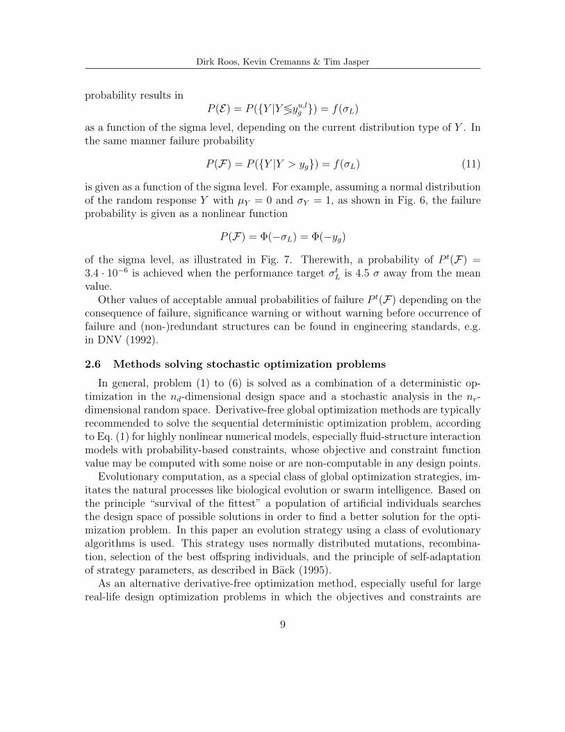
probability results inP (E) = P (Y |Y≶yu,lg ) = f(σL)

as a function of the sigma level, depending on the current distribution type of Y . Inthe same manner failure probability

P (F) = P (Y |Y > yg) = f(σL) (11)

is given as a function of the sigma level. For example, assuming a normal distributionof the random response Y with µY = 0 and σY = 1, as shown in Fig. 6, the failureprobability is given as a nonlinear function

P (F) = Φ(−σL) = Φ(−yg)

of the sigma level, as illustrated in Fig. 7. Therewith, a probability of P t(F) =3.4 · 10−6 is achieved when the performance target σtL is 4.5 σ away from the meanvalue.

Other values of acceptable annual probabilities of failure P t(F) depending on theconsequence of failure, significance warning or without warning before occurrence offailure and (non-)redundant structures can be found in engineering standards, e.g.in DNV (1992).

2.6 Methods solving stochastic optimization problems

In general, problem (1) to (6) is solved as a combination of a deterministic op-timization in the nd-dimensional design space and a stochastic analysis in the nr-dimensional random space. Derivative-free global optimization methods are typicallyrecommended to solve the sequential deterministic optimization problem, accordingto Eq. (1) for highly nonlinear numerical models, especially fluid-structure interactionmodels with probability-based constraints, whose objective and constraint functionvalue may be computed with some noise or are non-computable in any design points.

Evolutionary computation, as a special class of global optimization strategies, im-itates the natural processes like biological evolution or swarm intelligence. Based onthe principle “survival of the fittest” a population of artificial individuals searchesthe design space of possible solutions in order to find a better solution for the opti-mization problem. In this paper an evolution strategy using a class of evolutionaryalgorithms is used. This strategy uses normally distributed mutations, recombina-tion, selection of the best offspring individuals, and the principle of self-adaptationof strategy parameters, as described in Back (1995).

As an alternative derivative-free optimization method, especially useful for largereal-life design optimization problems in which the objectives and constraints are

9


Sensitivity analysisInitial design

Sensitive parametersIteration 0

Optimization

Optimal designIteration I, II, III, IV, ...

Modification ofsafety factors γ andconstraints um(d,γ)

Robustness evaluation

σL ∼= σtLσL ≶ σt

L

Reliability analysis

P (F) ∼= P t(F)P (F) ≶ P t(F)Robust and safety

optimal design

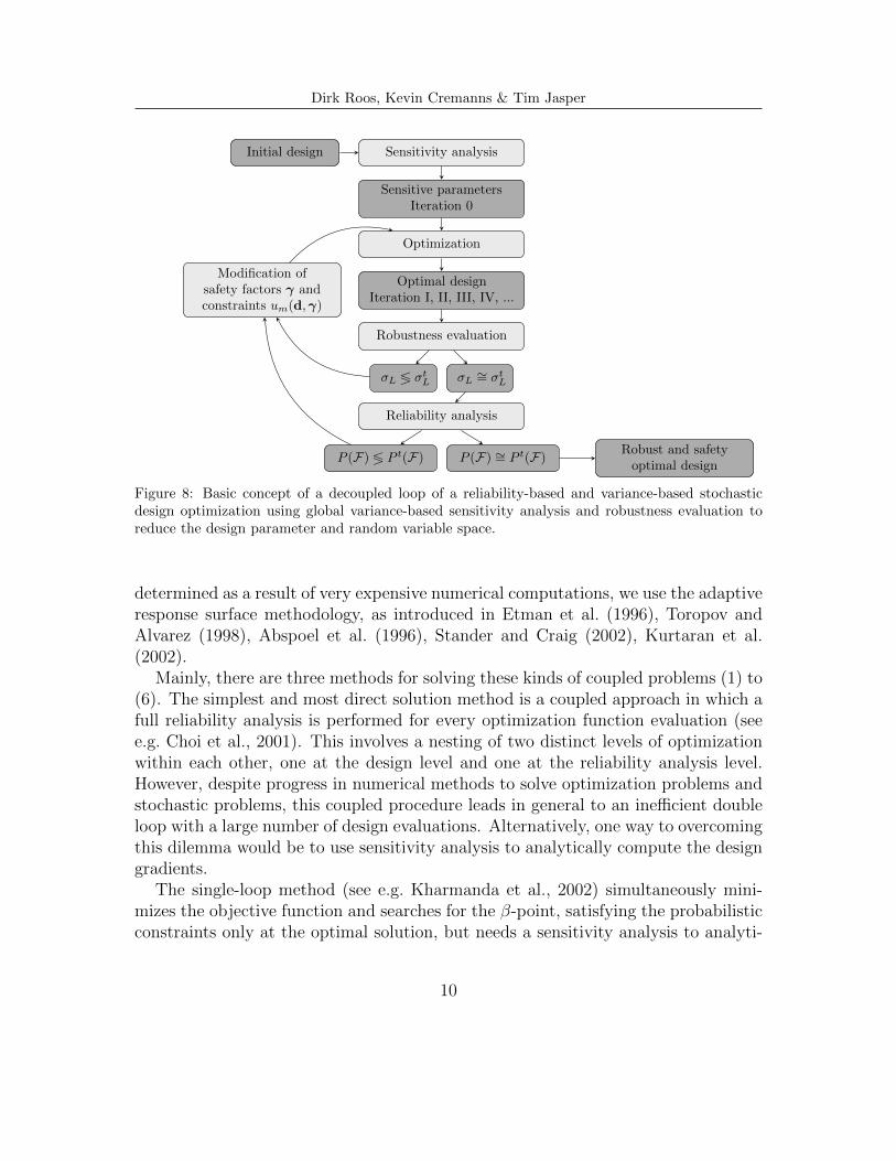
Figure 8: Basic concept of a decoupled loop of a reliability-based and variance-based stochasticdesign optimization using global variance-based sensitivity analysis and robustness evaluation toreduce the design parameter and random variable space.

determined as a result of very expensive numerical computations, we use the adaptiveresponse surface methodology, as introduced in Etman et al. (1996), Toropov andAlvarez (1998), Abspoel et al. (1996), Stander and Craig (2002), Kurtaran et al.(2002).

Mainly, there are three methods for solving these kinds of coupled problems (1) to(6). The simplest and most direct solution method is a coupled approach in which afull reliability analysis is performed for every optimization function evaluation (seee.g. Choi et al., 2001). This involves a nesting of two distinct levels of optimizationwithin each other, one at the design level and one at the reliability analysis level.However, despite progress in numerical methods to solve optimization problems andstochastic problems, this coupled procedure leads in general to an inefficient doubleloop with a large number of design evaluations. Alternatively, one way to overcomingthis dilemma would be to use sensitivity analysis to analytically compute the designgradients.

The single-loop method (see e.g. Kharmanda et al., 2002) simultaneously mini-mizes the objective function and searches for the β-point, satisfying the probabilisticconstraints only at the optimal solution, but needs a sensitivity analysis to analyti-

10


cally compute the design gradients of the probability constraint.An alternative method, used in the following, is the sequential approach (see e.g.

Chen et al., 2003). The general concept is to iterate between optimization and uncer-tainty quantification, updating the constraints based on the most recent probabilisticassessment results, using safety factors or other approximation methods. This effec-tive iterative decoupled loop approach can be enhanced by updating the constraintsduring the internal optimization using sigma levels and statistical moments

σLkσtL− 1 ≥ 0; σLk =

ygk − E[Yk]

σYk; k = 1, ng

in place of the exceedance probability of the Eq. (3). Essentially, by means of trans-formation in Eq. (11) of the probability-based highly nonlinear and non-differentiableconstraints to linear ones, these functions may be more well conditioned for the op-timization approach and we can expect a better performance of the solution process.Of course, the transformation in Eq. (11) can only be used as a rough estimationof the safety level and we have to calculate the probabilities of failure using thereliability analysis, at least at the iteration end.

As shown in Fig. 8, in the initial iteration step a variance-based sensitive analysisidentifies the most important multivariate dependencies and design parameters. Af-ter this, the deterministic optimization step results in an optimal solution for whichthe sigma level is calculated using a robustness evaluation, based on a latin hyper-cube sampling. The size of violation of the target sigma level is used to interpolatethe constraints using modified safety factors. Whereby, as an important fact, theinterpolation order increases continuously with each iteration step, so in practicethree or four iteration steps may meet our optimization requirements in terms ofrobustness and safety. Fig. 5 shows a typical convergence of a sequential stochasticchance-constrained optimization.

Furthermore, the optimization steps and the final reliability analysis run mostlyefficiently in the space of the current significant parameters. So every size of problemdefinition (number of design and random parameters) is solvable within all sigmalevels.

The following numerical example with a very high degree of complexity is givento demonstrate the solving power of this sequential stochastic chance-constrainedoptimization by adapting the constraint um(d, γ) depending on interpolated nominalresponse values yd.

11


Figure 9: Parametric CAD model of a one stage radial compressor, consisting of a impeller andreturnvane

3 NUMERICAL EXAMPLE

3.1 Computational fluid dynamics and process integration

Computational fluid dynamics (CFD) is an engineering method in which flowfields and other physics are calculated in detail for an application of interest. AN-SYS, which is used for the following example, uses a multidisciplinary approach tosimulation in which fluid flow models integrate seamlessly with other types of physicssimulation technologies.

Whereas, the CAE integration was carried out with the ANSYS Workbench en-vironment and optiPLug. The defined design and random parameters were modifiedwith the software optiSLang for binary-based CAE process integration, distributionof the parallel Workbench processes and for optimization and stochastic analysis.

3.2 Fluid-structure interaction model

The stochastic optimization method presented here is applied to a CAD and CAEparameter-based design optimization of a radial compressor shown in Fig. 9, includingmaterial, process and geometry tolerances. In the example presented the target of theoptimization process is to maximize the efficiency of the turbine engine with respectto a limitation of the maximal v. Mises stress. Additional constraints are defined byresonance of any eigen frequency with the rotational velocity of the rotor. In total

12


0.84

0.86

0.8890.893

0.9050.91

0 123 320 413 621667 873 945 1038 1236

N number of design evaluations

History of the efficiency η

SAN = 122

DO IARSM197

REI93

DO IIEA208

REII46

DO IIIEA206

REIII72

DO IVEA93

REIV142

ReliabilityanalysisN = 56

Efficiency of the initial design

Figure 10: Overview for the history of the efficiency η of all iterations. DO=deterministic optimiza-tion, RE=Robustness evaluation, EA= Evolutionary algorithm, ARSM=Adaptive response surfacemethod, SA=Sensitivity analysis

36 optimization parameters and 49 random influences are defined, as collected inTab. 2.

3.3 Decoupled stochastic optimization loop

In the following the optimization loop presented in Fig. 8 will be shown. Theinitial step starts with the sensitivity analysis, based on the so called meta modelsof optimal prognosis. Therefore, the most important multivariate dependencies anddesign parameters can be identified (see Eq. (9)). With these parameters identifiedfrom the sensitivity analysis, the number of parameters related to the optimizationproblem can be reduced. In our case up to 10 design variables are left over witha relevant coefficient of optimal prognosis. Furthermore the meta models of opti-mal prognosis can be used as a surrogate model for a pre-optimization. The meanefficiency of the initial radial compressor was 86%. The best design of the latinhypercube sampling with an efficiency of 88.9% is used as start design of an evo-lutionary optimization based on the surrogate model and gives with one additional

13


INEQUAL: lsc

1.751.51.2510.750.50.250INEQUAL: lsc [1e8]

21.

51

0.5

0P

DF

[1e-

8]

Fitted PDF

Histogram

Limit line

Statistic data

Min: 5.388e+007 Max: 1.737e+008

Mean: 1.106e+008 Sigma: 2.154e+007

CV: 0.1948

Skewness: 0.0605 Kurtosis: 2.924

Fitted PDF: Normal

Mean: 1.106e+008 Sigma: 2.154e+007

Limit x = 0

P_rel = 0 P_fit = 1.43132e-007

Probability P(X<x) = 0.95

x_rel = 1.4365e+008 x_fit = 1.45998e+008

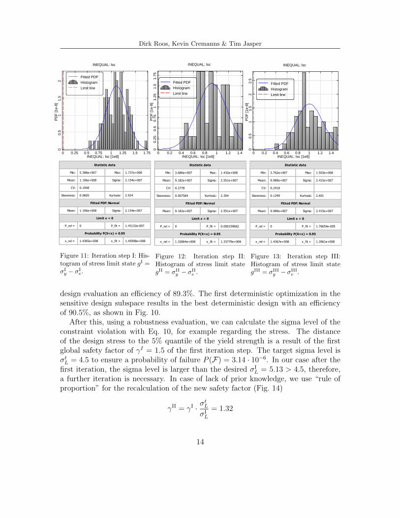
Figure 11: Iteration step I: His-togram of stress limit state gI =σIy − σI

e.

INEQUAL: lsc

1.41.210.80.60.40.20INEQUAL: lsc [1e8]

1.75

1.5

1.25

10.

750.

50.

250

PD

F [1

e-8]

Fitted PDF

Histogram

Limit line

Statistic data

Min: 3.686e+007 Max: 1.432e+008

Mean: 9.182e+007 Sigma: 2.551e+007

CV: 0.2778


Fitted PDF: Normal

Mean: 9.182e+007 Sigma: 2.551e+007

Limit x = 0

P_rel = 0 P_fit = 0.000159682


x_rel = 1.32864e+008 x_fit = 1.33779e+008

Figure 12: Iteration step II:Histogram of stress limit stategII = σII

y − σIIe .

INEQUAL: lsc

1.41.210.80.60.40.20INEQUAL: lsc [1e8]

2.5

21.

51

0.5

0P

DF

[1e-

8]

Fitted PDF

Histogram

Limit line

Statistic data

Min: 3.762e+007 Max: 1.503e+008

Mean: 9.989e+007 Sigma: 2.415e+007

CV: 0.2418


Fitted PDF: Normal

Mean: 9.989e+007 Sigma: 2.415e+007

Limit x = 0

P_rel = 0 P_fit = 1.76654e-005


x_rel = 1.4367e+008 x_fit = 1.3961e+008

Figure 13: Iteration step III:Histogram of stress limit stategIII = σIII

y − σIIIe .

design evaluation an efficiency of 89.3%. The first deterministic optimization in thesensitive design subspace results in the best deterministic design with an efficiencyof 90.5%, as shown in Fig. 10.

After this, using a robustness evaluation, we can calculate the sigma level of theconstraint violation with Eq. 10, for example regarding the stress. The distanceof the design stress to the 5% quantile of the yield strength is a result of the firstglobal safety factor of γI = 1.5 of the first iteration step. The target sigma level isσtL = 4.5 to ensure a probability of failure P (F) = 3.14 · 10−6. In our case after thefirst iteration, the sigma level is larger than the desired σI

L = 5.13 > 4.5, therefore,a further iteration is necessary. In case of lack of prior knowledge, we use “rule ofproportion” for the recalculation of the new safety factor (Fig. 14)

γII = γI · σtL

σIL

= 1.32

14


3

3.6

4.1

4.5

5.13

6

6.5

1.32 1.43 1.46 1.5 1.55

σL

γ

II III IV I

Figure 14: Interpolation of the global safety factor γ, de-pending on the estimated sigma level to modify the stressconstraint, Eq. (2).

INEQUAL: lsc

1.61.41.210.80.60.40.20INEQUAL: lsc [1e8]

21.

51

0.5

0P

DF

[1e-

8]

Fitted PDF

Histogram

Limit line

Statistic data

Min: 5.527e+007 Max: 1.622e+008

Mean: 1.004e+008 Sigma: 2.24e+007

CV: 0.2231


Fitted PDF: Normal

Mean: 1.004e+008 Sigma: 2.24e+007

Limit x = 0

P_rel = 0 P_fit = 3.70381e-006


x_rel = 1.42685e+008 x_fit = 1.37226e+008

Figure 15: Iteration step IV:Histogram of stress limit stategIV = σIV

y − σIVe .

The second deterministic optimization step increases the efficiency to 90.8% andthe second robustness evaluation with a new nominal design stress results in a newmean and standard deviation of the violation of the stress limit state as shown inFig. 12. But with these moments the new sigma level of σII

L = 3.6 turns out to be lessthan the predicted sigma level. Now with the prior knowledge of the first iteration,we can interpolate the new global safety factor to γIII = 1.426 with a new nominaldesign stress σIII

d = 1.75 · 108 for the third optimization.After the third iteration, we obtain a new efficiency of 90.9% and the third robust-

ness evaluation gives the following mean and standard deviation of the limit stateviolation shown in Fig. 13 with the new sigma level σIII

d = 4.1 < 4.5 near the targetvalue. In the iteration step III now the interpolation order is a quadratic one andthe new safety factor is γIV = 1.46. With the resulting new nominal design stressσIVd = 1.71 · 108

After the fourth iteration, we obtain the very best efficiency of 91%. In relation

15


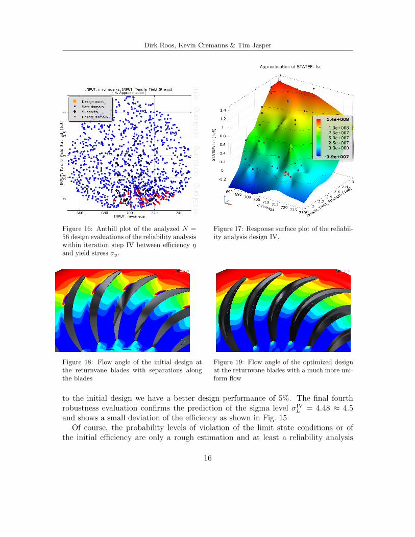
Figure 16: Anthill plot of the analyzed N =56 design evaluations of the reliability analysiswithin iteration step IV between efficiency ηand yield stress σy.

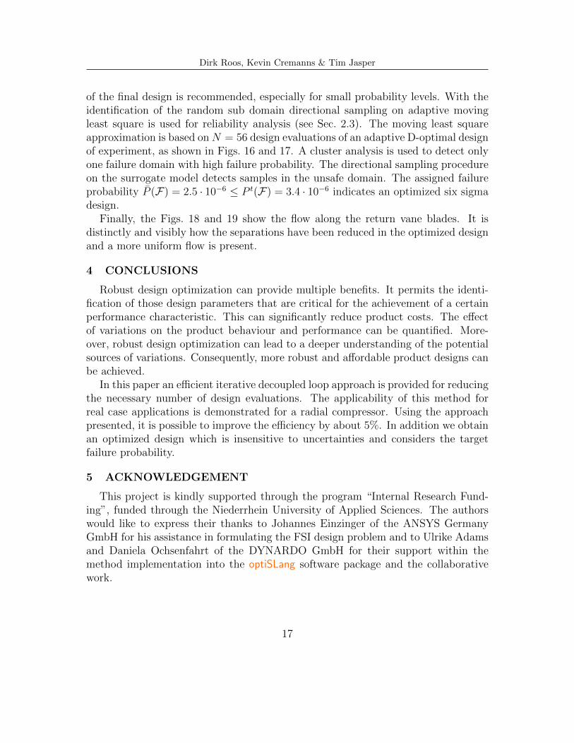
Figure 17: Response surface plot of the reliabil-ity analysis design IV.

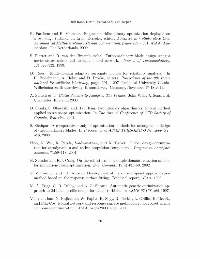
Figure 18: Flow angle of the initial design atthe returnvane blades with separations alongthe blades

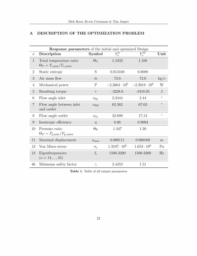
Figure 19: Flow angle of the optimized designat the returnvane blades with a much more uni-form flow

to the initial design we have a better design performance of 5%. The final fourthrobustness evaluation confirms the prediction of the sigma level σIV

L = 4.48 ≈ 4.5and shows a small deviation of the efficiency as shown in Fig. 15.

Of course, the probability levels of violation of the limit state conditions or ofthe initial efficiency are only a rough estimation and at least a reliability analysis

16


of the final design is recommended, especially for small probability levels. With theidentification of the random sub domain directional sampling on adaptive movingleast square is used for reliability analysis (see Sec. 2.3). The moving least squareapproximation is based onN = 56 design evaluations of an adaptive D-optimal designof experiment, as shown in Figs. 16 and 17. A cluster analysis is used to detect onlyone failure domain with high failure probability. The directional sampling procedureon the surrogate model detects samples in the unsafe domain. The assigned failureprobability P (F) = 2.5 · 10−6 ≤ P t(F) = 3.4 · 10−6 indicates an optimized six sigmadesign.

Finally, the Figs. 18 and 19 show the flow along the return vane blades. It isdistinctly and visibly how the separations have been reduced in the optimized designand a more uniform flow is present.

4 CONCLUSIONS

Robust design optimization can provide multiple benefits. It permits the identi-fication of those design parameters that are critical for the achievement of a certainperformance characteristic. This can significantly reduce product costs. The effectof variations on the product behaviour and performance can be quantified. More-over, robust design optimization can lead to a deeper understanding of the potentialsources of variations. Consequently, more robust and affordable product designs canbe achieved.

In this paper an efficient iterative decoupled loop approach is provided for reducingthe necessary number of design evaluations. The applicability of this method forreal case applications is demonstrated for a radial compressor. Using the approachpresented, it is possible to improve the efficiency by about 5%. In addition we obtainan optimized design which is insensitive to uncertainties and considers the targetfailure probability.

5 ACKNOWLEDGEMENT

This project is kindly supported through the program “Internal Research Fund-ing”, funded through the Niederrhein University of Applied Sciences. The authorswould like to express their thanks to Johannes Einzinger of the ANSYS GermanyGmbH for his assistance in formulating the FSI design problem and to Ulrike Adamsand Daniela Ochsenfahrt of the DYNARDO GmbH for their support within themethod implementation into the optiSLang software package and the collaborativework.

17


References

S.J. Abspoel, L.F.P. Etman, J. Vervoort, R.A. van Rooij, A.J.G Schoofs, and J.E.Rooda. Simulation based optimization of stochastic systems with integer designvariables by sequential multipoint linear approximation. Structural and Multidis-ciplinary Optimization, 22:125–138, 1996.

T. Back. Evolution strategies: an alternative evolutionary algorithm. In ArtificialEvolution, pages 3–20. Springer-Verlag, 1995.

A. Chateauneuf. Advances in solution methods for reliability-based design optimiza-tion, volume 1 of Structures and Infrastructures: Structural Design OptimizationConsidering Uncertainties, chapter 9, pages 217 – 246. Taylor & Francis, London,UK, 2008.

W. Chen, H. Liu, J. Sheng, and H. C. Gea. Application of the sequential optimizationand reliabilty assessment method to structural design problems. In Proceedings ofDETC’03, ASME 2003 Design Engineering Technical Conferences and Computersand Information in Engineering Conference, Chicao, Illinois USA, September 2 –6 2003.

K. K. Choi, J. Tu, and Y. H. Park. Extensions of design potential concept forreliability-based design optimization to nonsmooth and extreme cases. Structuraland Multidisciplinary Optimization, 22:335–350, 2001.

B. H. Dennis, G. S. Dulikravich, and Z.-X. Han. Constrined shape of optimization ofairfoil cascades using a navier-stokes solver and a genetic/sqp algorithm. In ASME99-GT-441, 1999.

O. Ditlevsen, R. E. Melchers, and H. Gluver. General multi-dimensional probabilityintegration by directional simulation. Computers & Structures, 36:355–368, 1990.

DNV. Structural reliability analysis of marine structure. Technical Report Classifica-tion Notes, No. 30.6, Det Norske Veritas Classification AS, Computer Typesettingby Division Ship and Offshore, Norway, 1992.

L.F.P. Etman, J.M.T.A. Adriaens, M.T.P. van Slagmaat, and A.J.G. Schoofs. Crash-worthiness design optimization using multipoint sequential linear programming.Structural Optimization, 12:222–228, 1996.

Victor E. Garzon. Probabilistic Aerothermal Design of Compressor Airfoils. PhDthesis, Massachusetts Institute of Technology, 2003.

18


Victor E. Garzon and David L. Darmofal. Impact of geometric variability on axialcompressor performance. Journal of Turbomachinery, 125:692–703, 2003.

T. Homma and A. Saltelli. Importance measures in global sensitivity analysis ofnonlinear models. Reliability Engineering & System Safety, 52(1):1 – 17, 1996.

D. E. Huntington and C. S. Lyrintzis. Improvements to and limitations of latinhypercube sampling. Probabilistic Engineering Mechanics, 13(4):245 – 253, 1998.

J. E. Hurtado. Structural robustness and its relationship to reliability, volume 1 ofStructures and Infrastructures: Structural Design Optimization Considering Un-certainties, chapter 16, pages 435 – 470. Taylor & Francis, London, UK, 2008.

G. Kharmanda, A. Mohamed, and M. Lemaire. Efficient reliability-based design opti-mization using a hybrid space withapplication to finite element analysis. Structuraland Multidisciplinary Optimization, 24:233 – 245, 2002.

H. Kurtaran, A. Eskandarian, D. Marzougui, and N.E. Bedewi. Crashworthinessdesign optimization using successive response surface approximations. Computa-tional Mechanics, 29:409–421, 2002.

A. Lange, M. Voigt, K. Vogeler, H. Schrapp, E. Johann, and V. Gummer. Prob-abilistic CFD simulation of a high-pressure compressor stage taking manufactur-ing variability into account. ASME Conference Proceedings, 2010(44014):617–628,2010.

T. Most. Efficient sensitivity analysis of complex engineering problems. In M. H.Faber, J. Kohler, and K. Nishijima, editors, 11th International Conference on Ap-plications of Statistics and Probability in Civil Engineering, Zurich, 2011. Balkema.

T. Most and J. Will. Metamodel of optimal prognosis - an automatic approach forvariable reduction and optimal metamodel selection. In Proceedings of the 5thWeimar Optimization and Stochastic Days, Weimar, Germany, November 20-21,2008. DYNARDO GmbH.

J. Muller-Tows. Aerodynamische Auslegung der Meridianstromung mehrstufiger Axi-alverdichter mit Hilfe von Optimierungsstrategien. PhD thesis, Universitat Kassel,2000.

A. Oyama. Multidisciplinary optimization of transonic wing design based on evolu-tionary algorithms coupled with cfd solver. In European Congress On Computa-tional Methods In Applied Sciences And Engineering, 2000.

19


R. Parchem and B. Meissner. Engine multidisciplinary optimization deployed ona two-stage turbine. In Ernst Kesseler, editor, Advances in Collaborative CivilAeronautical Multidisciplinary Design Optimization, pages 289 – 331. AIAA, Am-sterdam, The Netherlands, 2009.

S. Pierret and R. van den Braembussche. Turbomachinery blade design using anavier-stokes solver and artificial neural network. Journal of Turbomachinery,121:326–332, 1999.

D. Roos. Multi-domain adaptive surrogate models for reliability analysis. InH. Budelmann, A. Holst, and D. Proske, editors, Proceedings of the 9th Inter-national Probabilistic Workshop, pages 191 – 207. Technical University Carolo-Wilhelmina zu Braunschweig, Braunschweig, Germany, November 17-18 2011.

A. Saltelli et al. Global Sensitivity Analysis. The Primer. John Wiley & Sons, Ltd,Chichester, England, 2008.

D. Sasaki, S. Obayashi, and H.-J. Kim. Evolutionary algorithm vs. adjoint methodapplied to sst shape optimization. In The Annual Conference of CFD Society ofCanada, Waterloo, 2001.

S. Shahpar. A comparative study of optimisation methods for aerodynamic designof turbomachinery blades. In Proceedings of ASME TURBOEXPO Nr. 2000-GT-523, 2000.

Shyy, N. Wei, R. Papila, Vaidyanathan, and K. Tucker. Global design optimiza-tion for aerodynamics and rocket propulsion components. Progress in AerospaceSciences, 71:59–118, 2001.

N. Stander and K.J. Craig. On the robustness of a simple domain reduction schemefor simulation-based optimization. Eng. Comput., 19(4):431–50, 2002.

V. V. Toropov and L.F. Alvarez. Development of mars – multipoint approximationmethod based on the response surface fitting. Technical report, AIAA, 1998.

M. A. Trigg, G. R. Tubby, and A. G. Sheard. Automatic genetic optimization ap-proach to 2d blade profile design for steam turbines. In ASME 97-GT-392, 1997.

Vaidyanathan, N. Rajkumar, W. Papila, K. Shyy, R. Tucker, L. Griffin, Haftka N.,and Fitz-Coy. Neural network and response surface methodology for rocket enginecomponent optimization. AIAA, pages 2000–4880, 2000.

20


A DESCRIPTION OF THE OPTIMIZATION PROBLEM

Response parameters of the initial and optimized Designo Description Symbol Y 0

o Y IVo Unit

1 Total temperature ratioΘT = Tt,inlet/Tt,outlet

ΘT 1.1033 1.108

2 Static entropy S 0.013168 0.0088

3 Air mass flow m 72.6 72.6 kg/s

4 Mechanical power P −2.2664 · 106 −2.3918 · 106 W

5 Resulting torque τ -3238.8 -3418.05 J

6 Flow angle inlet αR1 2.2444 2.44

7 Flow angle between inletand outlet

αRS 62.562 67.63

8 Flow angle outlet αS1 22.009 17.13

9 Isentropic efficiency η 0.86 0.9094

10 Pressure ratioΘP = Pp,inlet/Pp,outlet

ΘP 1.347 1.38

11 Maximal displacement umax 0.000111 0.000169 m

12 Von Mises stress σe 1.3107 · 108 1.653 · 108 Pa

13 Eigenfrequencies(o = 14, ..., 45)

fi 1500-3200 1500-3200 Hz

46 Minimum safety factor γ 2.4453 1.51

Table 1: Table of all output parameters

21


Random variables Xj and design variables di of the initialand optimized Design; Φ =normal- Λ =log-normal distribution

j i Description Symbol d0i = dIVi = FX(x) σX

E[X]dli dui Unit

E[X0j ] E[X IV

j ]

01 01 Inlet width lin 53 50.35 Φ 0.1 47.7 58.3 mm

02 02 Exit width lex 26 26.27 Φ 0.1 23.4 28.6 mm

03 03 Radius of theimpeller

rimp 305 305.13 Φ 0.1 285 305 mm

04 - Totaltemperatureinlet

Tt,inlet 313 313 Φ 0.1 - - K

05 - Specific heatcapacity

Cp 1004.4 1004.4 Φ 0.1 - - J/kg/K

06 - Specific gasconstant

R 287.1 287.1 Φ 0.1 - - J/kg/K

07 - Massflow of theair at the inlet

m 72.6 72.6 Φ 0.1 - - kg/s

08 - Rotation speedof the impeller

Ω 699.76 699.76 Φ 0.1 - - radian/s

09 - Total pressureinlet

Pp,inlet 1724000 1724000 Φ 0.1 - - Pa

10 04 Angle variationalong hub of therotor

βRHB1 -48 -51.15 Φ -0.1 -52.8 -43.2


βRHB2 -25 -23.23 Φ -0.1 -27.5 -22.5


βRHB3 -25 -24.51 Φ -0.1 -27.5 -22.5

continued on next page ...

22




E[X]dli dui Unit

E[X0j ] E[X IV

j ]

13 07 Angle variationalong shroud of therotor

βRSB1 -55 -65.57 Φ -0.1 -60.5 -49


βRSB3 -30 -28.02 Φ -0.1 -33 -27


βRSB3 -45 -47.7 Φ -0.1 -49.5 -40.5

16 10 Thickness of therotor blades(shroud leadingedge)

tRSLE1 0.9 Φ 0.1 0.8 1.2 mm

17 11 (shroud trailingedge)

tRSTE6 5.95 Φ 0.1 5.0 7.0 mm

18 12 (hub trailing edge) tRHTE6 5.96 Φ 0.1 5.0 7.0 mm

19 13 (hub leading edge) tRHLE1 0.99 Φ 0.1 0.8 1.2 mm

20 14 Describes thecurvature of thevanes (hub)

βRVH1 60 71.54 Φ 0.1 54 66

21 15 Describes thecurvature of thevanes (shroud)

βRVS1 60 64.92 Φ 0.1 50 70

22 16 Relative thicknessof the returnvanealong the shroud

βRVS1 45 41.88 Φ 0.1 35 55 mm


23




E[X]dli dui Unit

E[X0j ] E[X IV

j ]

23 17 Relative thicknessof the returnvanealong the hub

βRVH1 45 43.42 Φ 0.1 45 66 mm

24 - Density of the steelmaterial

ρ 7850 7850 Φ 0.03 - - kg/m3

25 - Youngs modulus ofsteel

E 2 · 1011 2 · 1011 Λ 0.03 - -

26 - Poissons ratio ν 0.3 0.3 Λ 0.1 - -

27 - Coefficient ofthermal expansion

hc 1.2 · 10−5 1.2 · 10−5 Φ 0.04 - - C−1

28 - Referencetemperature

TRef 22 22 Φ 0.06 - - C

29 - Tensile yieldstrength

σy 2.5 · 108 2.5 · 108 Λ 0.064 - - Pa

30 - Compressive yieldstrength

σc 2.5 · 108 2.5 · 108 Λ 0.064 - - Pa


βRVS2 0 -0.36 Φ -0.1 -1 1


βRVS3 0 -0.56 Φ -0.1 -1 1

33 20 Relative thicknessof the returnvanealong the shroud

tRVS2 10 10.88 Φ 0.1 8 12 mm


24




E[X]dli dui Unit

E[X0j ] E[X IV

j ]

34 21 Relative thickness ofthe returnvane alongthe shroud

tRVS3 6 6 Φ 0.1 4.8 4.8 mm

35 22 Describes thecurvature of the vanes(hub)

βRVH2 0 -0.34 Φ -0.1 -1 1

36 23 Describes thecurvature of the vanes(hub)

βRVH3 0 -0.14 Φ -0.1 -1 1

37 24 Relative thickness ofthe returnvane alongthe hub

tRVH2 6 6.17 Φ 0.1 4.8 7.2 mm

38 25 Relative thickness ofthe returnvane alongthe hub

tRVH3 10 12 Φ 0.1 8 12 mm

39 26 Axial ratio of themajor axis to minoraxis of the ellipticalrounding of the inflowedge (hub)

rIEH 3 3.12 Φ 0.1 2.4 3.6


25




E[X]dli dui Unit

E[X0j ] E[X IV

j ]

40 27 Axial ratio of themajor axis to minoraxis of the ellipticalrounding of the inflowedge (shroud)

rIES3 3.14 Φ 0.1 2.4 3.6

41 28 Edge of the vane atthe leading edgealong the hub contour

rRVEHIn1 0.99 Φ 0.1 0.8 1.2

42 29 Edge of the vane atthe leading edge alongthe shroud contour

rRVESIn1 1 Φ 0.1 0.8 1.2

43 30 Edge of the vane atthe trailing edgealong the hub contour

rRVEHOut1 1.03 Φ 0.1 0.8 1.2

44 31 Edge of the vane atthe trailing edgealong the shroudcontour

rRVESOut1 1.18 Φ 0.1 0.8 1.2

45 32 Hub to shroud offsetimpeller

ξIHTSO0.5 0.53 Φ 0.1 0.4 0.6 %

46 33 Point toleranceimpeller

ξIPT0.1 0.08 Φ 0.1 0.08 0.12 %


26




E[X]dli dui Unit

E[X0j ] E[X IV

j ]

47 34 Hub to shroud offsetreturnvanve

ξRHTSO0.5 0.53 Φ 0.1 0.4 0.6 %

48 35 Point tolerancereturnvane

ξRPT0.1 0.08 Φ 0.1 0.08 0.12 %

49 36 Rounding of thetrailing edge

rTE 0.4 0.32 Φ 0.1 0.32 0.48 mm

Table 2: Table of all parameters

Constraints um(d) and objective f(d)Type Description Formula Unit

Constraint γ ≥ 1.5 u1(d) = γ − 1.5

Constraint Minimum ofΘP ≥ 1.34

u2(d) = ΘP − 1.34

Constraint Ω/2π needs to be±10% away of fi

u3(d) =|(fi−(Ω/2π))/(Ω/2π)|−0.1

Constraint Ω/π needs to be±10% away of fi

u4(d) =|(fi − (Ω/π))/(Ω/π)| − 0.1

Limit state condition Condition to calculatesigma level

g1(x) = σy − σe Pa

Objective Maximal efficiency(isentropic)

f(d) = η =(p2p1

)κ−1κ − 1

T2T1− 1

Table 3: Table of all constraints and objectives

27

Documents

PROBABILITY AND VARIANCE-BASED … deterministic optimization, ... usually stochastic programming algorithms or ... hensive study of the use of the combination of genetic algorithms