Embed Size (px)
Citation preview
Decomposition Algorithms for Global Solution of
Deterministic and Stochastic Pooling Problems in Natural
Gas Value Chains
by
Emre Armagan
Submitted to the Department of Mechanical Engineeringin partial fulfillment of the requirements for the degree of
Master of Science in Mechanical Engineering
at the
MASSACHUSETTS INSTITUTE OF TECHNOLOGY
January 2009
© Massachusetts Institute of Technology 2009. All rights reserved.
Author . . . . . . . . . . . . . . . . . . . . . . . . . . . . . . . . . . . . . . . . . . . . . . . .. . . . . . . . . . . . .Department of Mechanical Engineering
January 28, 2009
Certified by . . . . . . . . . . . . . . . . . . . . . . . . . . . . . . . . . . . . . . . . . .. . . . . . . . . . . . . . .Paul I. Barton
Professor, Department of Chemical EngineeringThesis Supervisor
Certified by . . . . . . . . . . . . . . . . . . . . . . . . . . . . . . . . . . . . . . . . . .. . . . . . . . . . . . . . .Stephen C. Graves
Professor, Department of Mechanical Engineering and ManagementThesis Supervisor
Accepted by. . . . . . . . . . . . . . . . . . . . . . . . . . . . . . . . . . . . . . . . . . .. . . . . . . . . . . . . .David E. Hardt
Chairman, Department Committee on Graduate Students

2
Decomposition Algorithms for Global Solution of Deterministic and
Stochastic Pooling Problems in Natural Gas Value Chains
by
Emre Armagan
Submitted to the Department of Mechanical Engineeringon January 28, 2009, in partial fulfillment of the
requirements for the degree ofMaster of Science in Mechanical Engineering
Abstract
In this thesis, a Benders decomposition algorithm is designed and implemented to solveboth deterministic and stochastic pooling problems to global optimality. Convergence ofthe algorithm to a global optimum is proved and then it is implemented both in GAMS andC++ to get the best performance. A series of example problems are solved, both with theproposed Benders decomposition algorithm and commerciallyavailable global optimiza-tion software to determine the validity and the performanceof the proposed algorithm.Moreover, a two stage stochastic pooling problem is formulated to model the optimal ca-pacity expansion problem in pooling networks and the proposed algorithm is applied tothis problem to obtain global optimum. A number of example stochastic pooling problemsare solved, both with the proposed Benders decomposition algorithm and commerciallyavailable global optimization software to determine the validity and the performance of theproposed algorithm applied to stochastic problems.
Thesis Supervisor: Paul I. BartonTitle: Professor, Department of Chemical Engineering
Thesis Supervisor: Stephen C. GravesTitle: Professor, Department of Mechanical Engineering and Management
3

4
Acknowledgments
First and foremost, I would like to thank my parents, Gulden and Kadri Armagan, for their
love and support. Without their help this degree would not have been possible.
I would like to thank my thesis supervisor Professor Paul I. Barton for his direction,
assistance, and guidance. His recommendations and suggestions have been invaluable for
the project and for this thesis. I am grateful to Professor Stephen C. Graves for reading and
evaluating my thesis.
I also wish to thank Professor Asgeir Tomasgard and Lars Hellemo from Norwegian
University of Science and Technology (NTNU). Professor Tomasgard’s assistance and sug-
gestions have been a tremendous help.
I am indebted to Ajay Selot who helped me whenever I need assistance and helped
me to learn necessary programming skills. In addition, I am also grateful to all of my
colleagues in the Process Systems Engineering Laboratory,especially Patricio Ramirez,
for their support and encouragement.
This research was supported by funding from StatoilHydro, SINTEF and NTNU. I
would like to thank them all for their financial support.
5

6

Contents
1 INTRODUCTION 15
1.1 POOLING PROBLEMS . . . . . . . . . . . . . . . . . . . . . . . . . . . 15
1.2 IMPORTANCE OFPOOLING PROBLEMS IN THE NATURAL GAS VALUE
CHAIN . . . . . . . . . . . . . . . . . . . . . . . . . . . . . . . . . . 17
1.3 BENDERSDECOMPOSITION FOR THEGLOBAL SOLUTION OF POOLING
PROBLEMS . . . . . . . . . . . . . . . . . . . . . . . . . . . . . . . . 19
2 PROBLEM DEFINITION 21
2.1 THE P-, Q- AND PQ-FORMULATIONS . . . . . . . . . . . . . . . . . . . 27
3 L ITERATURE REVIEW 31
3.1 DETERMINISTIC POOLING PROBLEM . . . . . . . . . . . . . . . . . . 31
3.2 INFRASTRUCTUREDEVELOPMENT AND THESTOCHASTICPOOLING PROB-
LEM . . . . . . . . . . . . . . . . . . . . . . . . . . . . . . . . . . . 34
4 BD ALGORITHM FOR DETERMINISTIC POOLING PROBLEM 39
4.1 INTRODUCTION OFBENDERSDECOMPOSITIONALGORITHM . . . . . . 39
4.2 PROOF OFCONVERGENCE . . . . . . . . . . . . . . . . . . . . . . . . 44
4.3 IMPLEMENTATION . . . . . . . . . . . . . . . . . . . . . . . . . . . . 48
4.3.1 GAMS IMPLEMENTATION . . . . . . . . . . . . . . . . . . . . 48
4.3.2 C++ IMPLEMENTATION . . . . . . . . . . . . . . . . . . . . . 54
7

4.3.3 RESULTS . . . . . . . . . . . . . . . . . . . . . . . . . . . . . 56
5 APPLICATION TO THE STOCHASTIC POOLING PROBLEM 59
5.1 INFRASTRUCTUREDEVELOPMENTPROBLEMS IN NATURAL GAS VALUE
CHAIN . . . . . . . . . . . . . . . . . . . . . . . . . . . . . . . . . . 59
5.2 INTRODUCTION TOSTOCHASTIC PROGRAMMING . . . . . . . . . . . . 61
5.3 IMPORTANCE OFSTOCHASTIC POOLING PROBLEMS IN NATURAL GAS
INFRASTRUCTUREDEVELOPMENT . . . . . . . . . . . . . . . . . . . 63
5.4 FORMULATION OF THE STOCHASTIC POOLING PROBLEM . . . . . . . . 65
5.5 IMPLEMENTATION OF THE BD ALGORITHM IN STOCHASTIC POOLING
PROBLEMS . . . . . . . . . . . . . . . . . . . . . . . . . . . . . . . . 71
5.6 RESULTS . . . . . . . . . . . . . . . . . . . . . . . . . . . . . . . . . 76
6 CONCLUSION 81
A EXAMPLE POOLING PROBLEMS 85
A.1 ADHYA’ S POOLING PROBLEM . . . . . . . . . . . . . . . . . . . . . . 85
A.2 FOULDS’ POOLING PROBLEM . . . . . . . . . . . . . . . . . . . . . . 87
A.3 EXAMPLE 1 . . . . . . . . . . . . . . . . . . . . . . . . . . . . . . . 89
A.4 EXAMPLE 2 . . . . . . . . . . . . . . . . . . . . . . . . . . . . . . . 89
A.5 EXAMPLE 3 . . . . . . . . . . . . . . . . . . . . . . . . . . . . . . . 89
A.6 EXAMPLE 4 . . . . . . . . . . . . . . . . . . . . . . . . . . . . . . . 90
B GAS NETWORK EXAMPLE 119
C THE STOCHASTIC POOLING PROBLEM 133
C.1 STOCHASTIC EXAMPLE 1 . . . . . . . . . . . . . . . . . . . . . . . . 134
C.2 STOCHASTIC EXAMPLE 2 . . . . . . . . . . . . . . . . . . . . . . . . 136
C.3 STOCHASTIC EXAMPLE 3 . . . . . . . . . . . . . . . . . . . . . . . . 138
C.4 STOCHASTIC EXAMPLE 4 . . . . . . . . . . . . . . . . . . . . . . . . 140
8
List of Figures
2-1 Graphical representation of a general pooling problem.. . . . . . . . . . . 22
2-2 Haverly’s pooling problem . . . . . . . . . . . . . . . . . . . . . . . . .. 25
2-3 The q-formulation of the Haverly’s pooling problem . . . .. . . . . . . . . 27
2-4 The pq-formulation of the Haverly’s pooling problem . . .. . . . . . . . . 28
4-1 Flowchart of the proposed BD algorithm . . . . . . . . . . . . . . . .. . . 46
4-2 The gas network example . . . . . . . . . . . . . . . . . . . . . . . . . . . 53
5-1 Basic illustration of decomposition algorithms in stochastic programming . 64
B-1 Representation of a mixer (a) and splitter (b) . . . . . . . . . . .. . . . . . 120
B-2 The gas network example . . . . . . . . . . . . . . . . . . . . . . . . . . . 120
9

10
List of Tables
2.1 Parameters of the pooling problem and corresponding definitions . . . . . . 23
2.2 Solution times for the p-,q- and pq- formulations in example problems (in
seconds). . . . . . . . . . . . . . . . . . . . . . . . . . . . . . . . . . . . 29
4.1 Optimal objective values in GAMS . . . . . . . . . . . . . . . . . . . .. . 50
4.2 Solution times in GAMS (in seconds) . . . . . . . . . . . . . . . . . .. . 51
4.3 Solution times for the gas network problem (in seconds) .. . . . . . . . . 53
4.4 Solution times in C++ with and without Range Reduction (in seconds) . . . 56
4.5 Solution times in C++ (in seconds) . . . . . . . . . . . . . . . . . . . .. . 56
5.1 Parameters and corresponding definitions for the first stage problem . . . . 68
5.2 Parameters and corresponding definitions for the secondstage problem . . . 69
5.3 Solution times of stochastic pooling problems with one quality variable (in
minutes) . . . . . . . . . . . . . . . . . . . . . . . . . . . . . . . . . . . . 78
5.4 Solution times of stochastic pooling problems with two quality variables
(in minutes) . . . . . . . . . . . . . . . . . . . . . . . . . . . . . . . . . . 78
5.5 Solution times of stochastic pooling problems with three quality variables
(in minutes) . . . . . . . . . . . . . . . . . . . . . . . . . . . . . . . . . . 78
A.1 Quality parameters in source nodes for Adhya’s problem .. . . . . . . . . 86
A.2 Cost parameters in source nodes for Adhya’s problem . . . . .. . . . . . . 86
A.3 Quality requirements in demand nodes for Adhya’s problem . . . . . . . . 86
11
A.4 Flow requirements in demand nodes for Adhya’s problem . .. . . . . . . . 86
A.5 Prices in demand nodes for Adhya’s problem . . . . . . . . . . . .. . . . 87
A.6 Quality parameters in source nodes for Foulds’ problem .. . . . . . . . . . 87
A.7 Cost parameters in source nodes for Foulds’ problem . . . . .. . . . . . . 88
A.8 Quality requirements in demand nodes for Foulds’ problem . . . . . . . . . 88
A.9 Flow requirements in demand nodes for Foulds’ problem . .. . . . . . . . 88
A.10 Prices in demand nodes for Foulds’ problem . . . . . . . . . . .. . . . . . 89
A.11 Quality parameters in source nodes for Example 1 . . . . . .. . . . . . . . 90
A.12 Cost parameters in source nodes for Example 1 . . . . . . . . . .. . . . . 91
A.13 Quality requirements in demand nodes for Example 1 . . . .. . . . . . . . 91
A.14 Flow requirements in demand nodes for Example 1 . . . . . . .. . . . . . 92
A.15 Prices in demand nodes for Example 1 . . . . . . . . . . . . . . . . .. . . 92
A.16 Quality parameters in source nodes for Example 2 . . . . . .. . . . . . . . 93
A.17 Cost parameters in source nodes for Example 2 . . . . . . . . . .. . . . . 94
A.18 Quality requirements in demand nodes for Example 2 . . . .. . . . . . . . 94
A.19 Flow requirements in demand nodes for Example 2 . . . . . . .. . . . . . 95
A.20 Prices in demand nodes for Example 2 . . . . . . . . . . . . . . . . .. . . 95
A.21 Quality parameters in source nodes for Example 3 . . . . . .. . . . . . . . 96
A.22 Cost parameters in source nodes for Example 3 . . . . . . . . . .. . . . . 96
A.23 Quality requirements in demand nodes for Example 3 . . . .. . . . . . . . 97
A.24 Flow requirements in demand nodes for Example 3 . . . . . . .. . . . . . 97
A.25 Prices in demand nodes for Example 3 . . . . . . . . . . . . . . . . .. . . 97
A.26 Quality parameters in source nodes for Example 4 . . . . . .. . . . . . . . 98
A.27 Cost parameters in source nodes for Example 4 . . . . . . . . . .. . . . . 98
A.28 Quality requirements in demand nodes for Example 4 . . . .. . . . . . . . 99
A.29 Flow requirements in demand nodes for Example 4 . . . . . . .. . . . . . 99
A.30 Prices in demand nodes for Example 4 . . . . . . . . . . . . . . . . .. . . 99
12
B.1 Quality parameters in source nodes for the gas network example . . . . . . 121
B.2 Cost parameters in source nodes for the gas network example. . . . . . . . 121
B.3 Quality requirements in demand nodes for the gas network example . . . . 121
B.4 Flow requirements in demand nodes for the gas network example . . . . . . 121
B.5 Prices in demand nodes for the gas network example . . . . . . .. . . . . 122
C.1 Source quality parameters in scenarios and the respective probability values 134
C.2 First stage investment costs of pools for Stochastic Example 1 . . . . . . . 134
C.3 First stage investment costs of pipelines (sources to pools) for Stochastic
Example 1 . . . . . . . . . . . . . . . . . . . . . . . . . . . . . . . . . . . 135
C.4 First stage investment costs of pipelines (pools to demands) for Stochastic
Example 1 . . . . . . . . . . . . . . . . . . . . . . . . . . . . . . . . . . . 135
C.5 Second stage cost parameters in source nodes for Stochastic Example 1 . . 135
C.6 Second stage quality requirements in demand nodes for Stochastic Exam-
ple 1 . . . . . . . . . . . . . . . . . . . . . . . . . . . . . . . . . . . . . . 135
C.7 Second stage flow requirements in demand nodes for Stochastic Example 1 135
C.8 Second stage prices in demand nodes for Stochastic Example 1 . . . . . . . 135
C.9 First stage investment costs of pools for Stochastic Example 2 . . . . . . . 136
C.10 First stage investment costs of pipelines (sources to pools) for Stochastic
Example 2 . . . . . . . . . . . . . . . . . . . . . . . . . . . . . . . . . . . 136
C.11 First stage investment costs of pipelines (pools to demands) for Stochastic
Example 2 . . . . . . . . . . . . . . . . . . . . . . . . . . . . . . . . . . . 136
C.12 Second stage cost parameters in source nodes for Stochastic Example 2 . . 137
C.13 Second stage quality requirements in demand nodes for Stochastic Exam-
ple 2 . . . . . . . . . . . . . . . . . . . . . . . . . . . . . . . . . . . . . . 137
C.14 Second stage flow requirements in demand nodes for Stochastic Example 2 137
C.15 Second stage prices in demand nodes for Stochastic Example 2 . . . . . . . 137
C.16 First stage investment costs of pools for Stochastic Example 3 . . . . . . . 138
13
C.17 First stage investment costs of pipelines (sources to pools) for Stochastic
Example 3 . . . . . . . . . . . . . . . . . . . . . . . . . . . . . . . . . . . 138
C.18 First stage investment costs of pipelines (pools to demands) for Stochastic
Example 3 . . . . . . . . . . . . . . . . . . . . . . . . . . . . . . . . . . . 138
C.19 Second stage cost parameters in source nodes for Stochastic Example 3 . . 139
C.20 Second stage quality requirements in demand nodes for Stochastic Exam-
ple 3 . . . . . . . . . . . . . . . . . . . . . . . . . . . . . . . . . . . . . . 139
C.21 Second stage flow requirements in demand nodes for Stochastic Example 3 139
C.22 Second stage prices in demand nodes for Stochastic Example 3 . . . . . . . 139
C.23 First stage investment costs of pools for Stochastic Example 4 . . . . . . . 140
C.24 First stage investment costs of pipelines (sources to pools) for Stochastic
Example 4 . . . . . . . . . . . . . . . . . . . . . . . . . . . . . . . . . . . 141
C.25 First stage investment costs of pipelines (pools to demands) for Stochastic
Example 4 . . . . . . . . . . . . . . . . . . . . . . . . . . . . . . . . . . . 141
C.26 Second stage cost parameters in source nodes for Stochastic Example 4 . . 142
C.27 Second stage quality requirements in demand nodes for Stochastic Exam-
ple 4 . . . . . . . . . . . . . . . . . . . . . . . . . . . . . . . . . . . . . . 142
C.28 Second stage flow requirements in demand nodes for Stochastic Example 4 142
C.29 Second stage prices in demand nodes for Stochastic Example 4 . . . . . . . 143
14

Chapter 1
Introduction
1.1 Pooling Problems
The pooling problem is a planning problem that arises in blending materials to produce
products; an example might be the blending of petroleum or natural gas. Pooling occurs
whenever streams are mixed together, often in a storage tank, and the resulting mixture is
distributed to several locations. Pooling and blending of raw materials and stored products
is an important step in the synthesis of end products having different quality specifications.
Products possessing different attribute qualities are mixed in a series of pools in such a way
that the attribute qualities of the blended products of the end pools must satisfy given re-
quirements. Pooling also occurs in distillation and other separation processes. The mathe-
matics of the pooling problem applies to such processes and their applications. In a pooling
problem, each material has a set of attributes with associated qualities, such as percentage
of sulfur or carbon dioxide percentage. Pool qualities are defined by a flow-weighted aver-
age of the source qualities and product qualities are similarly defined by a flow-weighted
average of the pool qualities. Product qualities are constrained to lie in specified ranges.
The pooling problem is to maximize the total profit, subject to flow and quality constraints.
The pooling problem is a bilinear optimization problem because the output stream qual-
15
ities, which are unknown, depend on the flowrates, which is also unknown, and on the
quality of the input streams. Because of the bilinear terms, the process of pooling intro-
duces nonlinearities and nonconvexities into optimization models leading to the possibility
of several locally optimal solutions some of which may be suboptimal. Naturally, it takes
more effort to solve a problem to guaranteed global optimality than it takes to find a locally
optimal solution and one must often weigh the benefits against the costs. However, it is ap-
parent that global optimization of the pooling and blendingprocess could lead to substantial
savings in cost, resulting in higher profits as in the case of the petroleum industry.
Numerical algorithms for solving pooling problems have included sensitivity and feasi-
bility analysis and local optimization techniques. However, because of the benefits of solv-
ing pooling problems to guaranteed global optimality as explained above, more recently
deterministic global optimization algorithms (which use Branch-and-Bound, Benders De-
composition (BD) or Generalized Benders Decomposition (GBD),etc.) have also been
proposed. However, the application of global optimizationalgorithms to the pooling prob-
lem continues to be a challenge because of the slow convergence speed of the proposed
algorithms. Since the nonconvexities and nonlinearities of a pooling problem come from
the bilinear terms, a BD or GBD based algorithm looks as a promising approach in order
to find the global optimal solution of the problem. Moreover,decomposition algorithms
are often regarded as better candidates to solve stochasticinfrastructure development prob-
lems in the natural gas value chains, which is the ultimate objective of this project. How-
ever, as explained in the later sections of this thesis, until now in the literature, in order
to solve pooling problems to global optimality with GBD algorithms (in the literature, a
BD algorithm has not yet been proposed for the solution of pooling problems), only one
of the variables appearing in the bilinear terms was taken asthe complicating variable (de-
tailed information about BD and GBD algorithms is provided inChapter 4) and with this
approach even for relatively simple pooling problems, the proposed GBD algorithms con-
verge to suboptimal solutions, even non-KKT points, and therefore does not guarantee a
16
global optimum.
1.2 Importance of Pooling Problems in the Natural Gas
Value Chain
Natural gas is a vital component of the world’s supply of energy and its importance has
been increasing as a fossil fuel in recent years because of different factors. First of all,
unlike other fossil fuels, natural gas is a relatively cleanfuel since it emits low levels of
potentially harmful byproducts such as sulphur particulates, carbon dioxide and nitrogen
oxides, as it burns. In addition, from the geographical perspective, natural gas is more
uniformly distributed than oil. Moreover, since it is relatively easy, cheap and clean to
convert it into hydrogen, natural gas is considered to be oneof the most important elements
in the transition to a hydrogen economy.
Raw natural gas typically consists primarily of methane (CH4), the shortest and lightest
hydrocarbon molecule. It also contains varying amounts of heavier gaseous hydrocarbons
(ethane (C2H6), propane (C3H8), butane (C4H10), etc.), acid gases (carbon dioxide (CO2),
hydrogen sulfide (H2S), etc.), nitrogen (N2), helium (He) and water vapor. All of those
gases except methane are called the impurities and the raw natural gas must be purified
to meet the quality standards specified by the contractual agreements between production
companies and major pipeline transmission and distribution companies. Those quality stan-
dards vary from pipeline to pipeline and are usually a function of a pipeline systems design
and the markets that it serves. In general, the standards specify that the natural gas be
within a specific range of heating value (For example, in the United States, it should be
about 1,035 ± 5% Btu per cubic foot of gas at 1 atmosphere and 60 °F); be delivered at
or above a specified hydrocarbon dew point temperature; be free of particulate solids and
liquid water to prevent erosion, corrosion or other damage to the pipeline; be dehydrated
of water vapor sufficiently to prevent the formation of methane hydrates within the gas
17
processing plant or pipeline; contain no more than trace amounts of components such as
hydrogen sulfide, carbon dioxide, nitrogen, and water vapor[10].
If natural gas is transported in the form of liquefied naturalgas (LNG), during LNG
production, the liquefaction process involves condensation of natural gas into liquid form
by cooling it to approximately −163 °C (−260 °F). The naturalgas fed into the LNG plant
has to be treated to remove water, hydrogen sulfide, carbon dioxide and other components
that will freeze under the low temperatures needed for storage or be destructive to the
liquefaction facility.
Moreover, with the advent of sustained higher natural gas prices and declining reserves,
and as technology and geological knowledge advances, so-called “unconventional” natural
gas sources are coming to market. Although, there are many different sources of “uncon-
ventional” natural gas today, one common characteristic ofall is the higher concentration
of acid gases compared to “conventional” natural gas sources. Therefore, as technology ad-
vances, large amounts of off-spec natural gas becomes available that does not meet pipeline
quality without some sort of adjustment. This off-spec gas has to be processed to meet the
requirements before being pumped into pipelines.
Hence, to transport natural gas from fields to consumers by any means or to make “un-
conventional” natural gas available to consumers, it is required to reduce the concentration
of undesired molecules. Two methods exist to achieve this goal: purification and blending.
The process of purification of natural gas to pipeline gas quality levels is quite complex,
highly capital-intensive and usually involves four main processes to remove the various
impurities: oil and condensate removal, water removal, separation of natural gas liquids,
sulfur and carbon dioxide removal. These processes become more complex and therefore
more expensive, as the concentration of the impurities increases in the natural gas being
purified and increases the cost of the natural gas for consumers while reducing the prof-
its of the production companies. Detailed information about purification processes can be
found in Guo and Ghambalor (2005) [17].
18
Blending of natural gas from different fields or wells with different different concentra-
tions of hydrocarbons, carbon dioxide, hydrogen sulfide andnitrogen is a cheaper method.
However, it does not always guarantee achievement of the desired concentration levels.
But, blending can be utilized to reduce the concentrations ofundesired molecules before
purification processes in order to reduce the cost of the purification. The opportunity for
blending different sources of natural gas comes into the picture especially when the natural
gas production infrastructure is being developed. When new wells or fields are being de-
veloped, it is possible to construct the pipeline system such that the gas from different wells
are mixed together to satisfy the requirements for different qualities. However to develop
the pipeline system optimally, a stochastic version of the pooling problem where the qual-
ity parameters in the wells are not known exactly has to be solved. Although advancing
technology provides the necessary tools to predict the gas content of natural gas in different
fields during the exploration stage, the impurities in the natural gas are still uncertain before
drilling the well. Thus, stochastic programming principles have to be used to achieve an
optimum solution to the infrastructure development problem. As mentioned, in this study,
one of the important reasons to develop a BD algorithm to solvepooling problems is the
adaptability of decomposition algorithms to stochastic programming. More information
about the stochastic pooling problem is given inChapter 5of this thesis.
1.3 Benders Decomposition for the Global Solution of Pool-
ing Problems
As explained inSection 4.1, BD and GBD algorithms are proposed to solve multi-variable
nonlinear programs and take at least one of the variables appearing in bilinear terms as
fixed to solve the problem. In the literature, in order to solve pooling problems to global
optimality with GBD, only one of the variables appearing in the bilinear terms was taken as
the complicating variable. With this approach, even for relatively simple pooling problems,
19

the GBD algorithm tends to generate suboptimal points and does not guarantee to attain a
global optimum. For instance, Floudas & Aggarwal (1990) [11] use the GBD algorithm to
solve pooling problems by fixing the pool quality variables as the complicating variables
and decompose the original pooling problem into a primal problem and a relaxed master
problem. But, their strategy is only successful for Haverly’s pooling problem (which is a
very simple problem) and in general, it offers no guarantee for global optimality. This GBD
algorithm may converge to a local minimum, a local maximum, or even a non-KKT point.
In this study, both of the variables appearing in bilinear terms are treated as the com-
plicating variables and by doing so the problem can be formulated such that the Benders
Decomposition algorithm can be used instead of GeneralizedBenders Decomposition and
hence satisfaction of the Property P becomes unnecessary and, unlike Floudas & Aggarwal
(1990) [11], convergence is guaranteed and can be proven directly from Benders (1962)
[5]. Fixing both variables in the bilinear terms provides a linear program in the first stage
of the algorithm and smaller (and hence easier to solve) bilinear second stage problems. For
comparison of the proposed algorithm with a well known and respected global solver, The
Branch And Reduce Optimization Navigator (BARON) is selected[42]. BARON is a com-
putational software developed by Nikolaos Sahinidis and Mohit Tawarmalani for solving
nonconvex optimization problems to global optimality. Purely continuous, purely integer,
and mixed-integer nonlinear problems can be solved with this software. BARON com-
bines constraint propagation, interval analysis, range (domain) reduction and duality with
enhanced Branch-and-Bound (B+B) concepts to solve optimization problems globally. In
general, BARON is a nonconvex optimization solver using range reduction methods in-
tegrated into the B+B algorithm with advanced relaxation techniques [39]. In this study,
in order to check global optimality and validity of the approach, various example pooling
problems are solved with both the proposed BD algorithm and BARON. In addition, the
solution times of the BD algorithm and BARON are compared to study the overall perfor-
mance of BD for pooling problems.
20

Chapter 2
Problem Definition
In general, the pooling problem can be stated in a general wayas follows: given several
streams with different qualities, what quantities of each must be mixed in intermediate
pools in such a way that the quality and quantity requirements of all demands are satisfied.
A pooling network consists of several source nodes, pools and end-product nodes. Each
source node has a unique quantity of available supply and quality components. Sources are
linked to pools and each pool represents a blend from varioussource nodes and the quality
component of a pool is a function of the levels of in-flows fromsources and their qualities.
Pools are linked to product nodes and each pool’s total in-flow is equal to its total out-flow
(mass balance). The quality component of a product node is also a function of the levels of
in-flows from sources and pools and their qualities. Productnodes are subject to specific
demand and quality requirements. In practice, because of the presence of a large number of
supply nodes, pools, qualities and end-products, pooling problems are more complicated
than expected. Usually, each stream into a pool can have morethan one quality compo-
nent. The pooling problem then becomes a problem with multiple component qualities and
every end product has to be in the range of expected quality specifications for each of the
quality components. The existence of multiple pools, products and qualities creates hun-
dreds of bilinear terms even for a relatively small problem and therefore a large number of
21
suboptimal local minima can also exist, hence the need for a global optimization approach
increases.
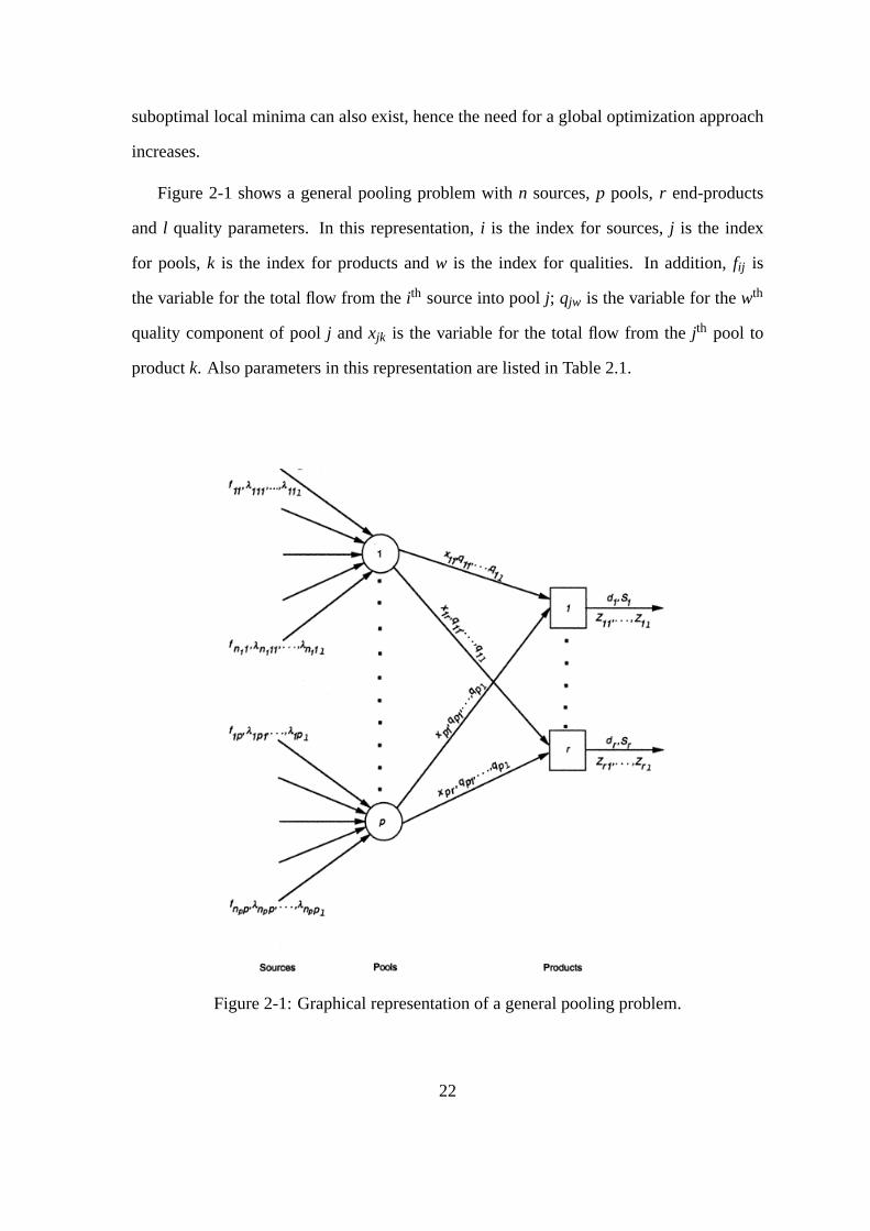
Figure 2-1 shows a general pooling problem withn sources,p pools, r end-products
and l quality parameters. In this representation,i is the index for sources,j is the index
for pools,k is the index for products andw is the index for qualities. In addition,fij is
the variable for the total flow from theith source into poolj; qjw is the variable for thewth
quality component of poolj andxjk is the variable for the total flow from thejth pool to
productk. Also parameters in this representation are listed in Table2.1.
Figure 2-1: Graphical representation of a general pooling problem.
22

Parameter Definition
cij cost of the flow from theith source into poolj
dk unit price of productk
l total number of component qualities
N j set of sources entering poolj
p total number of pools
r total number of end-products
Sk demand requirement for productk
Zkw wthquality requirement for productk
λ ijw wth quality component of the flow from theith source into poolj
Table 2.1: Parameters of the pooling problem and corresponding definitions
Then, a mathematical representation of the general poolingproblem that is represented
in Figure 2-1 becomes:
minf ,x,q
p
∑j=1
∑i∈Nj
ci j fi j −r
∑k=1
dk
p
∑j=1
x jk (2.1)
s.t. ∑i∈Nj
fi j −r
∑k=1
x jk = 0, j = 1, ..., p (2.2)
q jw
r
∑k=1
x jk − ∑i∈Nj
λi jw fi j = 0, j = 1, ..., p; w = 1, ..., l (2.3)
p
∑j=1
x jk −Sk ≤ 0, k = 1, ..., r (2.4)
p
∑j=1
q jwx jk −Zkw
p
∑j=1
x jk ≤ 0, k = 1, ..., r; w = 1, ..., l (2.5)
23
f Li j ≤ fi j ≤ fU
i j , i = 1, ...,n j ; j = 1, ..., p
qLjw ≤ q jw ≤ qU
jw, j = 1, ..., p; w = 1, ..., l
xLjk ≤ x jk ≤ xU
jk, j = 1, ..., p; k = 1, ..., r
In this formulation, the objective function represents thedifference between the cost
of the flow from the source nodes and the returns from selling the end-products. (2.2)
represents the mass balances for each pool. (2.3) expressesthe mass balance for each
quality component. (2.4) ensures that the flows to each end-product node do not exceed
the demands. (2.5) enforces that the quality requirements are satisfied at each end-product
node. More information about the formulation can be found inAudet et. al. (2004) [3].
In addition, in the literature there are some widely known and solved pooling problem
formulations which are just special cases of this general representation. These problems
are solved in numerous papers about the pooling problem and hence their global optimal
solutions are known and there are different global optimization algorithms, which have
already been proven to converge, available for them, which can be used for comparison with
the BD algorithm. Thus, these problems can be used as examplesto check the validity and
performance of the proposed BD algorithm. The pooling problem was first investigated by
Haverly (1978-1979) [19, 20]. Therefore, Haverly’s pooling problem is one of these widely
known pooling problems and it consists of only 3 source nodes, 1 pool and 2 demand nodes
as shown in Figure 2-2. Figure clearly represents that threefeed streams are available (f1,
f2 and f3), with the costs of $6, $16 and $10 (per unit) respectively. There are also two
output streams with the prices of $9 and $15 (per unit) respectively.
In Haverly’s pooling problem, there is a single pool which receives supplies from two
different sources which have different sulfur qualities. Athird supply is not connected to
24
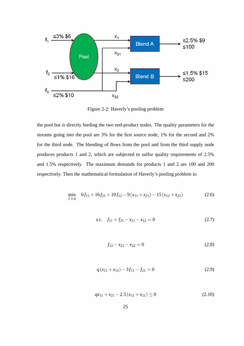
Figure 2-2: Haverly’s pooling problem
the pool but is directly feeding the two end-product nodes. The quality parameters for the
streams going into the pool are 3% for the first source node, 1%for the second and 2%
for the third node. The blending of flows from the pool and fromthe third supply node
produces products 1 and 2, which are subjected to sulfur quality requirements of 2.5%
and 1.5% respectively. The maximum demands for products 1 and 2 are 100 and 200
respectively. Then the mathematical formulation of Haverly’s pooling problem is:
minf ,x,q
6 f11+16f21+10f12−9(x11+x21)−15(x12+x22) (2.6)
s.t. f11+ f21−x11−x12 = 0 (2.7)
f12−x21−x22 = 0 (2.8)
q(x11+x12)−3 f11− f21 = 0 (2.9)
qx11+x21−2.5(x11+x21) ≤ 0 (2.10)
25
qx12+2x22−1.5(x12+x22) ≤ 0 (2.11)
x11+x21 ≤ 100
x12+x22 ≤ 200
whereq is the sulfur quality of the pool output,fij are the quantities of supplies,x11 and
x12 are the magnitude of flows from pool to end-products andx21 andx22 are the magnitude
of flows from the third source node to end-products. Similar to the general formulation, the
objective function represents the difference between the cost of the flow from the source
nodes and the returns from selling the end-products. (2.7) and (2.8) represent the mass
balance. (2.9) represents the sulfur mass balance. (2.10) and (2.11) expresses the quality
restrictions on the products; (2.12) and (2.13) ensure thatthe flows to each end-product
node do not exceed the demands. GAMS implementation of Haverly’s pooling problem is
provided inAppendix A.
As it can be realized, although the objective function is linear, the bilinear terms in (2.9),
(2.10) and (2.11) introduce nonconvexities in the problem (which are enough to make this
problem nonconvex) causing multiple local optima. Therefore, local nonlinear program-
ming (NLP) solution algorithms (well known examples are SNOPT, MINOS, CONOPT,
etc.) may provide suboptimal solutions which are usually not useful in any practical sense
and hence it is necessary to explore global optimization techniques in pooling problems.
In this study, also Adhya’s [1] and Foulds’ [12] pooling problems are solved to test
the BD algorithm. Since they are just special versions of the general formulation, it is
not necessary to give explicit formulations for those problems, just the numbers of pools,
sources, qualities and end-products should be enough to produce an explicit formulation
by using the general problem formulation. For Adhya’s problem, the number of pools
26
is 7; the number of sources is 8, the number of qualities is 4 and the number of end-
products is 4; in Foulds’ problem, the number of pools is 8; the number of sources is 14,
the number of qualities is 1 and the number of end-products is6. More information for both
of these example problems including quality specs, demand requirements, cost coefficients
and GAMS implementations are given inAppendix A.
2.1 The p-, q- and pq-Formulations
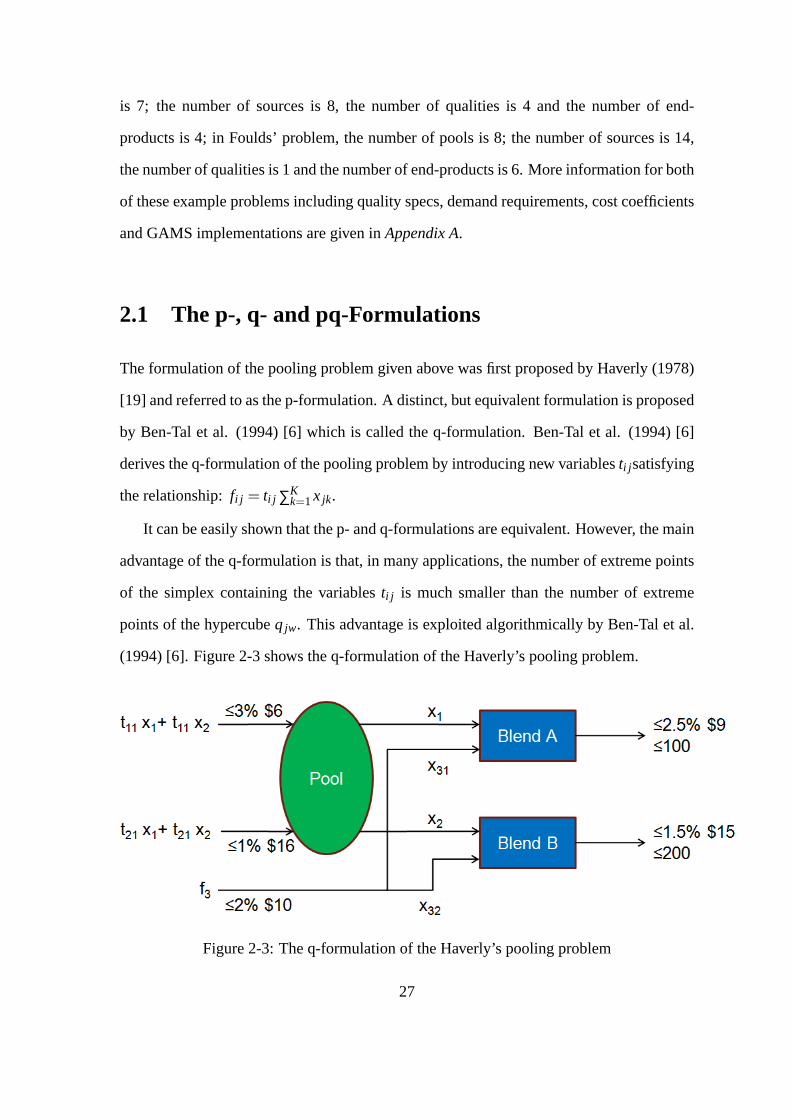
The formulation of the pooling problem given above was first proposed by Haverly (1978)
[19] and referred to as the p-formulation. A distinct, but equivalent formulation is proposed
by Ben-Tal et al. (1994) [6] which is called the q-formulation. Ben-Tal et al. (1994) [6]
derives the q-formulation of the pooling problem by introducing new variablesti j satisfying
the relationship:fi j = ti j ∑Kk=1x jk.
It can be easily shown that the p- and q-formulations are equivalent. However, the main
advantage of the q-formulation is that, in many applications, the number of extreme points
of the simplex containing the variablesti j is much smaller than the number of extreme
points of the hypercubeq jw. This advantage is exploited algorithmically by Ben-Tal et al.
(1994) [6]. Figure 2-3 shows the q-formulation of the Haverly’s pooling problem.
Figure 2-3: The q-formulation of the Haverly’s pooling problem
27

Tawarmalani & Sahinidis (2002) [45] constructs the pq-formulation by adding the fol-
lowing constraint to the q-formulation:
I
∑i=1
ti j x jk = x jk, j = 1, ..., p; k = 1, ..., r (2.12)
Figure 2-4 illustrates the pq-formulation of the Haverly’spooling problem. As can be
realized from this example, the newly added constraints areredundant and don’t change the
feasible region. However, the main point of interest in the pq-formulation is the tightness
of the convex relaxations relative to the other two formulations. Tawarmalani&Sahinidis
(2002) [45] prove that the pq-formulation provides much tighter convex relaxations com-
pared to the p- and q-formulations.
Figure 2-4: The pq-formulation of the Haverly’s pooling problem
Tawarmalani & Sahinidis (2002) [45] claim that for all example pooling problems, the
pq-formulation decreases solution times drastically and solution times of example pooling
problems (solved with BARON) presented in [45] to prove thisstatement. However, in
[45] the chart provided for comparison of three formulations in terms of solution times
does feature solutions from different references and therefore with different processors and
hence the validity of their claims can be questioned. Therefore, it is decided to model
three example pooling problems (Haverly’s [18], Foulds’ [12] and Adhya’s [1]) with all
28
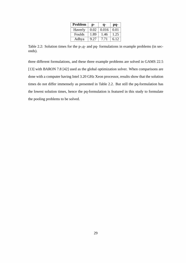
Problem p- q- pq-Haverly 0.02 0.016 0.01Foulds 1.89 1.46 1.25Adhya 9.27 7.71 6.12
Table 2.2: Solution times for the p-,q- and pq- formulationsin example problems (in sec-onds).
three different formulations, and these three example problems are solved in GAMS 22.5
[13] with BARON 7.8 [42] used as the global optimization solver. When comparisons are
done with a computer having Intel 3.20 GHz Xeon processor, results show that the solution
times do not differ immensely as presented in Table 2.2. But still the pq-formulation has
the lowest solution times, hence the pq-formulation is featured in this study to formulate
the pooling problems to be solved.
29

30
Chapter 3
Literature Review
3.1 Deterministic Pooling Problem
Various optimization procedures for the pooling problem have been proposed in the liter-
ature. These solution procedures can be classified based on their convergence to either a
local or a global optimum. The first algorithm for the poolingproblem was suggested by
Haverly (1978-1979) [19, 20]. Haverly’s approach was basedon the idea of using recursion
to solve the pooling problem. A recursive approach guesses the value of the pool qualities.
These values for the pool qualities converts the pooling problem into a linear program in
the flow variables. The actual values of the pool qualities can then be calculated from the
values of the flow variables that are obtained by solving the linear program. The process
continues until the actual values of the qualities are within a range of tolerance from the
guessed values. The main drawback in using any form of recursive method for the pooling
problem is that often the algorithm does not converge to a solution, and when it converges,
it converges only to a local minimum, a local maximum, or evena non-KKT point. In addi-
tion, as the number of pools and end-products increases, recursive methods tend to become
more unstable, resulting in computational difficulties.
Successive Linear Programming (SLP) approaches which solve nonlinear problems as
31
a sequence of linear programs are also widely used. Lasdon (1979) [31] proposes an al-
gorithm based on SLP technique. These approaches also do notguarantee global optimal
solutions and may converge to even a non-KKT point .
As in the case of GBD, decomposition methods are based on the observation that a dif-
ficult problem can be converted to an easier problem by fixing values of certain variables.
In the case of the pooling problem, for example, fixing the pool quality variables converts
it into a linear program. By using this approach, Floudas & Aggarwal (1990) [11] sug-
gest an algorithm based on fixing the pool quality variables as the complicating variables
and decomposing the original pooling problem into a primal problem and a relaxed master
problem and iterating between these problems based on the GBDalgorithm until the termi-
nation conditions are satisfied. Although their decomposition strategy is successful for the
problems suggested by Haverly, in general it offers no guarantee for global optimality. This
GBD algorithm may converge to a local minimum, a local maximum, or even a non-KKT
point. Visweswaran & Floudas (1996) [50] propose a GOP algorithm for solving the pool-
ing problem. The algorithm was proven to terminate finitely with a global optimum. Using
this algorithm, the authors were able to solve three cases ofthe Haverly problem. It is
also reported that a single pool, five-product problem, witheach stream having two quality
components is solved to global optimality using this algorithm. Large-scale pooling prob-
lems, generated randomly, having up to 5 pools, 5 products, and 30 qualities, were solved
by Androulakis et al. (1996) [2] using a different implementation of the GOP algorithm.
Branch-and-bound (B+B) methods for pooling and blending problems have been sug-
gested by different authors. These methods usually differ in the relaxations used to provide
valid lower bounds to the global optimum. Foulds et al. (1992) [12] use a procedure which
involves replacing the bilinear terms in the pooling problem by their McCormick (1983)
[35] concave and convex envelopes. The nonlinear pooling problem can be relaxed to a
linear programming problem, the solution of which providesa lower bound on the global
optimal solution. The B+B procedure proceeds by partitioning the feasible set and relaxing
32

on each partition. It is quite obvious that by replacing eachbilinear term by its concave
or convex envelope introduces a relaxation, but this relaxation also tends to zero as the
partitions get finer and the algorithm converges to the global optimal solution. Using this
approach, Foulds et al. (1992) [12] were able to solve single-quality problems, with the
largest problem having 8 pools and 14 products. The constraints which provide the convex
and concave envelopes of the problem at a specific node of the B+B tree are not in general
valid for other nodes of the tree. Thus, the convex and concave envelopes have to be gener-
ated at each node of the B+B tree. However, the McCormick relaxation requires four linear
constraints to provide the envelopes for each bilinear termin the problem. Hence, as the
number of pools, products, or component qualities increase, the size of the linear program
to be solved at each node of the B+B tree also increases.
Ben-Tal et al. (1994) [6] propose another lower-bounding procedure based on La-
grangian relaxation of another formulation of the pooling problem (explained in the pre-
vious chapter as the q-formulation). In this paper, a B+B algorithm which partitions the
feasible set of the pooling problem is provided and it is shown that this approach can reduce
the duality gap between a nonconvex problem and its dual. Later it is also proven that for
partially convex problems such as the pooling problem, under certain regularity conditions,
this approach can reduce the duality gap between the primal and the dual to zero.
Adhya et al. (1999) [1] use yet another formulation of the pooling problem (explained
in the previous chapter as the pq-formulation). The authorsprovide a new Lagrangian
relaxation approach for developing lower bounds for the B+B to solve the pooling problem
and it is proven that the Lagrangian relaxation approach provides tighter lower bounds than
the standard linear-programming relaxations used in global optimization algorithms and
hence guarantees faster convergence speeds.
33
3.2 Infrastructure Development and the Stochastic Pool-
ing Problem
For the infrastructure development problem, most of the literature is on oil production
planning and unfortunately there is only small amount of literature dealing specifically with
natural gas production planning, but usually modeling and solution strategies for oil and
gas infrastructure development problems are very similar.Hence, no distinction is made
between the oil and gas production planning literature, andthe literature for oil production
planning is also included to this review.
Most of the available literature for planning of oil and gas field infrastructures uses a de-
terministic approach without considering how uncertaintyaffects the overall system (Iyer,
Grossmann, Vasantharajan & Cullick (1998) [22]; Van den Heever & Grossmann (2000)
[47]; Van den Heever & Grossmann (2001) [48]; Barnes, Linke & Kokossis (2002) [4]; Lin
& Floudas (2003) [32]; Ortiz-Gomez, Rico-Ramirez & Hernandez-Castro (2002) [37]). For
a recent review of the existing literature on deterministicapproaches for these problems, re-
fer to Van den Heever & Grossmann (2001) [48]. Recently, therehas been some work that
considers uncertainty in the infrastructure development problem. Jonsbraten (1998) [24]
presents an MILP model for optimizing the investment and operation decisions for an oil-
field under uncertainty in oil prices. The author uses the Progressive Hedging Algorithm
to solve the problem. Jonsbraten (1998ii) [25] presents an implicit enumeration algorithm
for the sequencing of oil wells under uncertainty in oil reserves. The decision models for
both these papers include investment and operational decisions for one field only. Jornsten
(1992) [27] uses Lagrangian relaxation of constraints to solve a stochastic program for the
sequencing of gas fields under uncertainty in future demands. The author assumes that
production profiles and capacities of platforms have already been fixed. Haugen (1996)
[18] proposes a single parameter representation for uncertainty in the size of reserves and
incorporates it into a Stochastic Dynamic Programming model for scheduling of petroleum
34

fields. This work also assumes that the only decisions that need to be made are regarding
the scheduling of fields. Meister, Clark, and Shah (1996) [36]present a model to derive
exploration and production strategies for one field under uncertainty in reserves and future
oil price. The model is analyzed using stochastic control techniques. Lund (2000) [33]
presents a stochastic dynamic programming model for evaluating the value of flexibility in
offshore development projects under uncertainty in futureoil prices and in the reserves of
one field. Jonsbraten (1998iii) [26] discusses an interesting problem dealing with planning
of oil field development. A situation is considered where twosurface lease owners with
access to the same oil reservoir bargain their shares of production. The author assumes
a mixed-integer optimization model and uses game theory. Recently, there has also been
some work using real options based approaches (Dias, 2001 [9]) for planning of oil and gas
field developments under uncertainty.
Based on the dependence of the stochastic process on the decisions, Jonsbraten (2001)
[27] and Goel & Grossmann (2004) [15] classify uncertainty in planning problems into
two categories: project exogenous uncertainty and projectendogenous uncertainty. Prob-
lems where the stochastic process is independent of the project decisions are said to have
project exogenous uncertainty. For these problems, the scenario tree is fixed and does not
depend on the decisions. Hence the most relevant characteristic of this kind of stochastic
programming model is that its formulation assumes a given scenario tree. The uncertainty
in gas prices in a planning problem similar to the one described here is an example of
project exogenous uncertainty. For recent reviews on models and solution techniques for
stochastic programs with project exogenous uncertainty, please refer to Kall and Wallace
(1994) [29] and Birge and Louveaux (1997) [7]. Problems wherethe project decisions in-
fluence the stochastic process are said to possess project endogenous uncertainty. A gas
production planning problem with uncertainty in gas reserves is included in this category.
This is because the uncertainty in gas reserves of a field is resolved only if, and when,
exploration or investment is done at the field. If no action istaken, the uncertainty in the
35
field does not resolve at all. For problems with project endogenous uncertainty, the sce-
nario trees are decision-dependent. This leads to difficulties in defining the model because,
traditionally, the stochastic programming literature hasrelied on the assumption of given
scenario trees. Hence, there is very little literature dealing with problems having process
endogenous uncertainty. An intensive literature search provides only four papers (Pflug,
(1990) [38]; Jonsbraten, Wets & Woodruff, (1998) [24]; Jonsbraten, (1998ii) [25]; Goel &
Grossmann, (2004) [15]) which deal with project endogenousuncertainty.
A Literature review clearly shows that none of the literature about the infrastructure
development problem considers the concentrations of the impurities in the natural gas pro-
duced as a source of uncertainty, but as mentioned in the firstchapter, because of the con-
tractual agreements, regulations and the pipeline requirements, the production company has
to adjust the composition of the gas within some limits to sell it, and the composition of
gas is unknown when infrastructure is being developed. To blend gas from different fields,
while the infrastructure is being developed, the pipeline system has to be constructed to
allow the gas from different wells to be mixed to satisfy the requirements. Therefore, to
develop the value chain optimally, a stochastic version of the pooling problem where the
quality parameters in the wells are unknown has to be solved.Therefore, gas quality un-
certainty in the infrastructure development problem is selected in this study as the first step
to construct and solve a realistic model of the whole infrastructure development problem
with more realistic or less assumptions than the literatureuntil now.
Another important assumption in the literature is that the effect of the contractual frame-
work is not considered. However, in most fields natural gas cannot be produced unless a
contractual demand exists and in addition the rules given incontracts and also in govern-
mental regulations need to be taken into account to reach a realistic model of the system. In
addition, there are other important assumptions: no expansion in capacity of a platform is
considered; in most of the references production rate decreases linearly in time; flow mod-
els and reservoir models are assumed as linear and more importantly effects of contractual
36

framework are neglected.
37

38
Chapter 4
BD Algorithm for Deterministic Pooling
Problem
4.1 Introduction of Benders Decomposition Algorithm
The Benders Decomposition algorithm was originally proposed by Benders in 1962 [5] for
nonlinear, nonconvex mixed variables programming problems of the form:
maxx,y
cTx+ f (y) (4.1)
s.t. Ax+F(y) ≤ 0 (4.2)
x∈ X ⊂ Rnx,y∈U ⊂ R
ny
wherey is a vector of complicating variables, since the problem above can be solved
more easily wheny is fixed constant. In other words, for fixedy, this problem separates
into a number of smaller problems each having only subsets ofx as variable or the problem
assumes a special structure, such as a linear program as in the case of the pooling problem
39

or the problem is converted into a convex program. In these cases, by fixingy, a simpler
primal problem can be solved and a relaxed master problem is solved to generate valid
lower bounds and the algorithm converges to the global optimum by iterating between these
problems. In practice, the BD algorithm decomposes problem into two smaller problems:
primal problem (linear program) and relaxed master problem(nonlinear program in bilinear
problems). The primal problem is used to find the upper bound (UBD); the relaxed master
problem is used to find the lower bound (LBD). When LBD≥UBD, algorithm terminates.
On the other hand, the Generalized Benders Decomposition algorithm is first proposed
by Geoffrion (1972) [14] and also based on Benders Decomposition, but it is proposed to
solve more general form of nonconvex nonlinear programs of the form:
maxx,y
f (x,y) (4.3)
s.t. g(x,y) ≤ 0 (4.4)
x∈ X ⊂ Rnx,y∈U ⊂ R
ny
wherey is a vector of complicating variables, again, in the sense that it is much easier to
solve inx wheny are held fixed. However, the problem to be solved has to satisfy a property
called ”Property P”, unlike Benders Decomposition. Basically, the problem to be solved
has to be formulated such that for everyλ ≥ 0, (whereλs are the Lagrange multipliers),
the infimum of f (x,y)+ λ Tg(x,y)) overX can be taken essentially independently ofy, so
that the constraints in the relaxed master problem can be obtained explicitly with little or
no more effort than is required to evaluate it at a single value ofy.
As it is known, bilinear terms are formed by the multiplication of two variables of the
problem and these bilinear terms introduce nonconvexitiesto the problem. If the noncon-
vexities in the problem are only introduced by the bilinear terms, as in the case of pooling
40
problems, it is possible to treat the whole bilinear terms asa complicating variable in the
BD algorithm as opposed to fixing only one of the variables in bilinear terms as the com-
plicating variable. Fixing the bilinear terms yields constant parameters. Then, the general
formulation of the pooling problem can be written (consistently to the notation given in
Chapter 2) as:
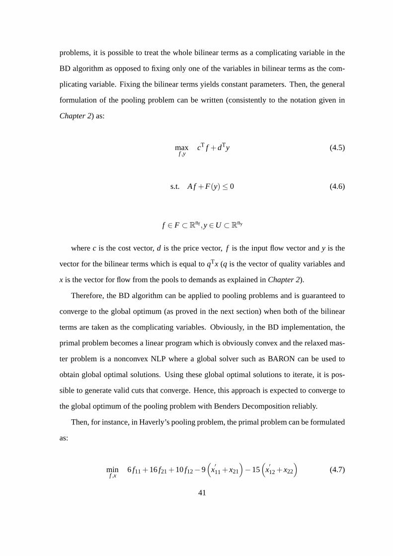
maxf ,y
cT f +dTy (4.5)
s.t. A f +F(y) ≤ 0 (4.6)
f ∈ F ⊂ Rnf ,y∈U ⊂ R
ny
wherec is the cost vector,d is the price vector,f is the input flow vector andy is the
vector for the bilinear terms which is equal toqTx (q is the vector of quality variables and
x is the vector for flow from the pools to demands as explained inChapter 2).
Therefore, the BD algorithm can be applied to pooling problems and is guaranteed to
converge to the global optimum (as proved in the next section) when both of the bilinear
terms are taken as the complicating variables. Obviously, in the BD implementation, the
primal problem becomes a linear program which is obviously convex and the relaxed mas-
ter problem is a nonconvex NLP where a global solver such as BARON can be used to
obtain global optimal solutions. Using these global optimal solutions to iterate, it is pos-
sible to generate valid cuts that converge. Hence, this approach is expected to converge to
the global optimum of the pooling problem with Benders Decomposition reliably.
Then, for instance, in Haverly’s pooling problem, the primal problem can be formulated
as:
minf ,x
6 f11+16f21+10f12−9(
x′
11+x21
)
−15(
x′
12+x22
)
(4.7)
41

s.t. f11+ f21−x′
11−x′
12 = 0 (4.8)
f12−x21−x22 = 0 (4.9)
q′(
x′
11+x′
12
)
−3 f11− f21 = 0 (4.10)
q′x′
11+x21−2.5(
x′
11+x21
)
≤ 0 (4.11)
q′x′
12+2x22−1.5(
x′
12+x22
)
≤ 0 (4.12)
whereq′, x
′
11 andx′
12 are constant parameters which are assigned as the fixed compli-
cated variables. Therefore, bilinearities in the primal problem disappear and it becomes
a linear program and therefore, it is convex. However, the relaxed master problem is still
a bilinear program and it is obviously a nonconvex NLP. Hence, still the relaxed master
problem has to be solved with a global solver such as BARON. But, the potential benefit of
utilizing BD algorithm might be to solve number of smaller problems (the relaxed master
problems) with the B+B procedure (such as BARON) instead of solving one huge prob-
lem with the B+B. B+B based algorithms are exponential-time algorithms. In other words,
as the problem size increases, solution times of B+B algorithms increases exponentially.
Therefore, instead of solving a problem with large number ofvariables, solving number of
problems with small number of variables can be quicker in terms of the solution times.
As mentioned, the primal problem becomes a linear program and general formulation
of the primal problem becomes:
42
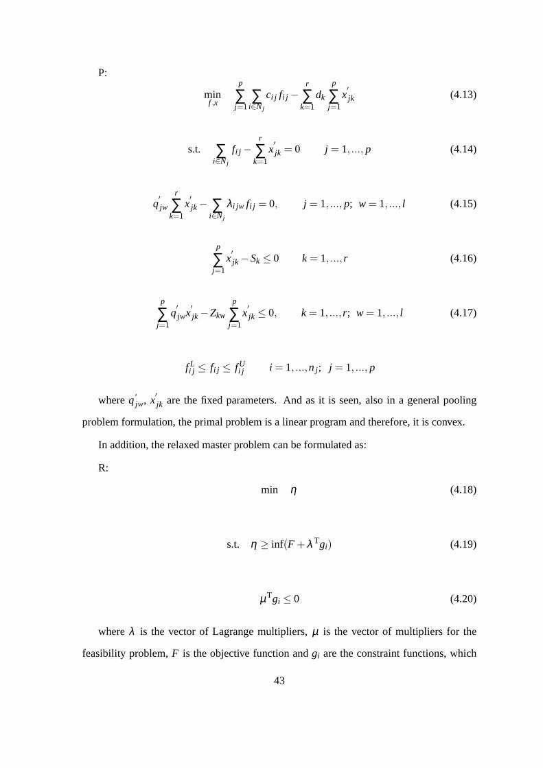
P:
minf ,x
p
∑j=1
∑i∈Nj
ci j fi j −r
∑k=1
dk
p
∑j=1
x′
jk (4.13)
s.t. ∑i∈Nj
fi j −r
∑k=1
x′
jk = 0 j = 1, ..., p (4.14)
q′
jw
r
∑k=1
x′
jk − ∑i∈Nj
λi jw fi j = 0, j = 1, ..., p; w = 1, ..., l (4.15)
p
∑j=1
x′
jk −Sk ≤ 0 k = 1, ..., r (4.16)
p
∑j=1
q′
jwx′
jk −Zkw
p
∑j=1
x′
jk ≤ 0, k = 1, ..., r; w = 1, ..., l (4.17)
f Li j ≤ fi j ≤ fU
i j i = 1, ...,n j ; j = 1, ..., p
whereq’jw, x
′
jk are the fixed parameters. And as it is seen, also in a general pooling
problem formulation, the primal problem is a linear programand therefore, it is convex.
In addition, the relaxed master problem can be formulated as:
R:
min η (4.18)
s.t. η ≥ inf(F +λ Tgi) (4.19)
µTgi ≤ 0 (4.20)
whereλ is the vector of Lagrange multipliers,µ is the vector of multipliers for the
feasibility problem,F is the objective function andgi are the constraint functions, which
43

means:
F =p
∑j=1
∑i∈Nj
ci j fi j −r
∑k=1
dk
p
∑j=1
x jk (4.21)
g1 = ∑i∈Nj
fi j −r
∑k=1
x jk, j = 1, ..., p (4.22)
g2 = q jw
r
∑k=1
x jk − ∑i∈Nj
λi jw fi j , j = 1, ..., p; w = 1, ..., l (4.23)
g3 =p
∑j=1
x jk −Sk ≤ 0 k = 1, ..., r (4.24)
g4 =p
∑j=1
q jwx jk −Zkw
p
∑j=1
x′
jk ≤ 0, k = 1, ..., r; w = 1, ..., l (4.25)
Then, the proposed BD algorithm for pooling problems is presented in Algorithm 1
and also flowchart of the algorithm is provided in Figure 4-1.As Figure 4-1 represents,
basically, The primal problem provides the upper bound value (UBD) whereas the relaxed
master problem provides the lower bound value (LBD) and when LBD≥UBD, algorithm
terminates.
By using this algorithm, different pooling problems from theliterature are solved and
validity and speed of this approach is tested versus algorithms which guarantees global
optimal solution such as BARON. However, before testing thealgorithm, the first step is to
prove its convergence to global optimum.
4.2 Proof of Convergence
To prove the convergence of the proposed algorithm, the firststep is to show that the pooling
problem formulation satisfies the form given by Benders (1962) [5]:
44
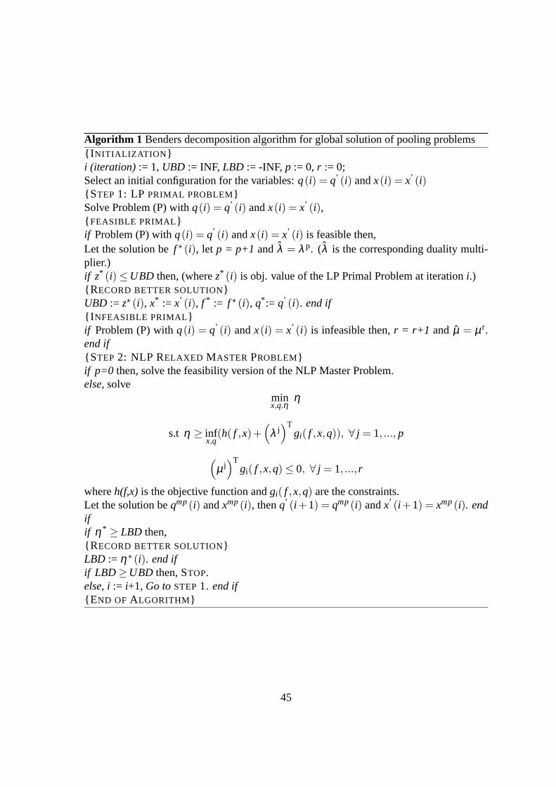
Algorithm 1 Benders decomposition algorithm for global solution of pooling problems{I NITIALIZATION }i (iteration) := 1, UBD := INF, LBD := -INF, p := 0, r := 0;Select an initial configuration for the variables:q(i) = q’ (i) andx(i) = x’ (i){STEP 1: LP PRIMAL PROBLEM}Solve Problem (P) withq(i) = q’ (i) andx(i) = x’ (i),{ FEASIBLE PRIMAL}if Problem (P) withq(i) = q’ (i) andx(i) = x’ (i) is feasible then,Let the solution bef ⋆ (i), let p = p+1 andλ = λ p. (λ is the corresponding duality multi-plier.)if z* (i) ≤UBD then, (wherez* (i) is obj. value of the LP Primal Problem at iterationi.){R ECORD BETTER SOLUTION}UBD := z⋆ (i), x* := x’ (i), f * := f ⋆ (i), q* := q’ (i). end if{I NFEASIBLE PRIMAL}if Problem (P) withq(i) = q’ (i) andx(i) = x’ (i) is infeasible then,r = r+1 and µ = µ r.end if{STEP 2: NLP RELAXED MASTER PROBLEM}if p=0 then, solve the feasibility version of the NLP Master Problem.else, solve
minx,q,η
η
s.t η ≥ infx,q
(h( f ,x)+(
λ j)T
gi( f ,x,q)), ∀ j = 1, ..., p
(
µ j)T
gi( f ,x,q) ≤ 0, ∀ j = 1, ..., r
whereh(f,x) is the objective function andgi( f ,x,q) are the constraints.Let the solution beqmp(i) andxmp(i), thenq’ (i +1) = qmp(i) andx’ (i +1) = xmp(i). endifif η* ≥ LBD then,{R ECORD BETTER SOLUTION}LBD := η⋆ (i). end ifif LBD ≥UBD then, STOP.else, i:= i+1, Go toSTEP1. end if{E ND OF ALGORITHM}
45
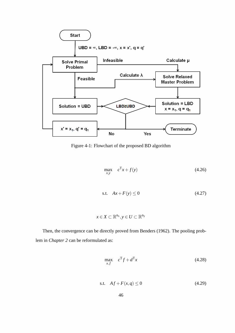
Figure 4-1: Flowchart of the proposed BD algorithm
maxx,y
cTx+ f (y) (4.26)
s.t. Ax+F(y) ≤ 0 (4.27)
x∈ X ⊂ Rnx,y∈U ⊂ R
ny
Then, the convergence can be directly proved from Benders (1962). The pooling prob-
lem inChapter 2can be reformulated as:
maxx, f
cT f +dTx (4.28)
s.t. A f +F(x,q) ≤ 0 (4.29)
46

f ∈ F ⊂ Rnf ,x∈ X ⊂ R
Tx,q∈ Q⊂ RTq
The crucial point in satisfying Benders (1962) [5] formulation and hence proving con-
vergence is when the complicating variables are fixed, the resulting formulation has to be a
linear program. Since in the proposed algorithm bothx andq (bilinear terms) are fixed as
complicating variables. The resulting formulation in the pooling problem is:
maxx, f
cT f +B (4.30)
s.t. A f +C≤ 0 (4.31)
f ∈ F ⊂ Rnf
whereB = dTx, C = F(x, q) andx andq are fixed parameters. It is obvious that the re-
sulting formulation is a linear program and hence it can be concluded that proof of conver-
gence for the proposed BD algorithm can be derived directly from the proof of convergence
of Benders original algorithm.
Benders (1962) [5] states that the problem given in the form of(4.28) and (4.29) can be
written in the equivalent form by introducing a scalar variable f0:
max{
f0| f0−cT f −dTx≤ 0, A f +F(x,q) ≤ 0, x≥ 0}
(4.32)
In other words,(
f0, f , x, q)
is an optimum solution of problem if and only iff0 =
cT f +dTy and(
f , x, q)
is an optimum solution of the problem.
Theorem 3.1 (Partitioning Theorem for mixed-variables) ofBenders (1962) [5] proves
that (a)(
f , x, q)
is an optimum solution of problem denoted by (4.29) and (4.30) if and only
if(
f0, f , x, q)
is an optimum solution of (4.33). In addition, this theorem shows that (b) if
47

(
f , x, q)
is an optimum solution of (4.32), andf0 = cT f +dTy then(
f0, x, q)
is an optimum
solution of (4.32) andf is an optimum solution of the linear programming problem:
max{
cT f |A f ≤−F(x,q), x≥ 0}
(4.33)
Also, the same theorem proves that (c) if(
f0, x, q)
is an optimum solution of (4.32),
then (4.33) is feasible and the optimum value of the objective function in this problem is
equal to f0−F(x, q). If f is an optimum solution of (4.33), then(
f , x, q)
is an optimum
solution of the original problem.
(a), (b) and (c) of the Partitioning Theorem for mixed variables show that a two stage
algorithm fixingx andq as complicating variables converges to the global optimum the
mixed variable problem in the form of (4.28) and (4.29).
4.3 Implementation
After convergence is proved, the next step is to implement the algorithm. The GAMS lan-
guage is powerful enough for reasonably complex algorithms. Hence, at first GAMS is
chosen to implement the proposed BD algorithm. GAMS Version 22.5 [13] is used as the
implementation language and as mentioned before both BARON(Version 7.8) [42] and
the BD algorithm is implemented as the global solvers for the example pooling problems.
However, because of the reasons explained in the next section, the algorithm is reimple-
mented in C++ with first using a custom B+B solver to solve the relaxed master problem
in the BD implementation, then using a callable BARON C++ library and the results are
compared with BARON alone as the global solver of the poolingproblem.
4.3.1 GAMS Implementation
In GAMS, both problem specific formulations and the general formulation are implemented
in order to check if there is a problem with the general formulation. Fortunately, the imple-
48
mentation of the general problem shown is not different fromthe problem specific imple-
mentations. In this project, Haverly’s pooling problem andalso Adhya’s [1] and Foulds’
[12] pooling problems are solved to test the proposed BD algorithm.
The GAMS implementation of the BD algorithm is provided inAppendix Ain addi-
tion to the GAMS implementations of the example problem formulations. It is quite well
known that the optimal objective value of Haverly’s poolingproblem -400. This value is
also confirmed by the BARON implementation and the proposed BDalgorithm gives the
same objective value as the solution. In addition, the BD implementation is tested with
several different starting points and it is observed that for all tested starting points, it con-
verges to the global optimal solution (only the number of iterations changes, hence solution
times also change slightly). Hence, it can be stated that, the BD algorithm is working for
Haverly’s pooling problem without any problem and converges to a global optimum.
The algorithm is also tested with Fould’s [12] pooling problem with 8 pools, 14 sources,
1 quality and 6 end-products. BARON converges to -52 as the optimal objective value and
also the proposed BD algorithm gives the same optimal objective value. Again, the BD
implementation is tested with several different starting points for Fould et al.’s pooling
problem and it is observed that for all tested starting points, it converges to the global
optimal solution.
Another test problem is Adhya’s [1] pooling problem with 7 pools, 8 sources, 4 qualities
and 4 end-products. BARON converges to -1185 as the optimal objective value and also the
proposed BD algorithm gives the same optimal objective value. Again, the BD implemen-
tation is tested with several different starting points forAdhya et al.’s pooling problem and
it is observed that for all tested starting points, it converges to the global optimal solution.
In addition, 4 example pooling problems (which were createdby the author) are also
solved. More information for both of these example problemsincluding quality specs,
demand requirements, cost coefficients and GAMS implementations are given inAppendix
A. Example 1 has 14 pools, 18 sources, 1 quality and 9 end-products. The BD solver
49
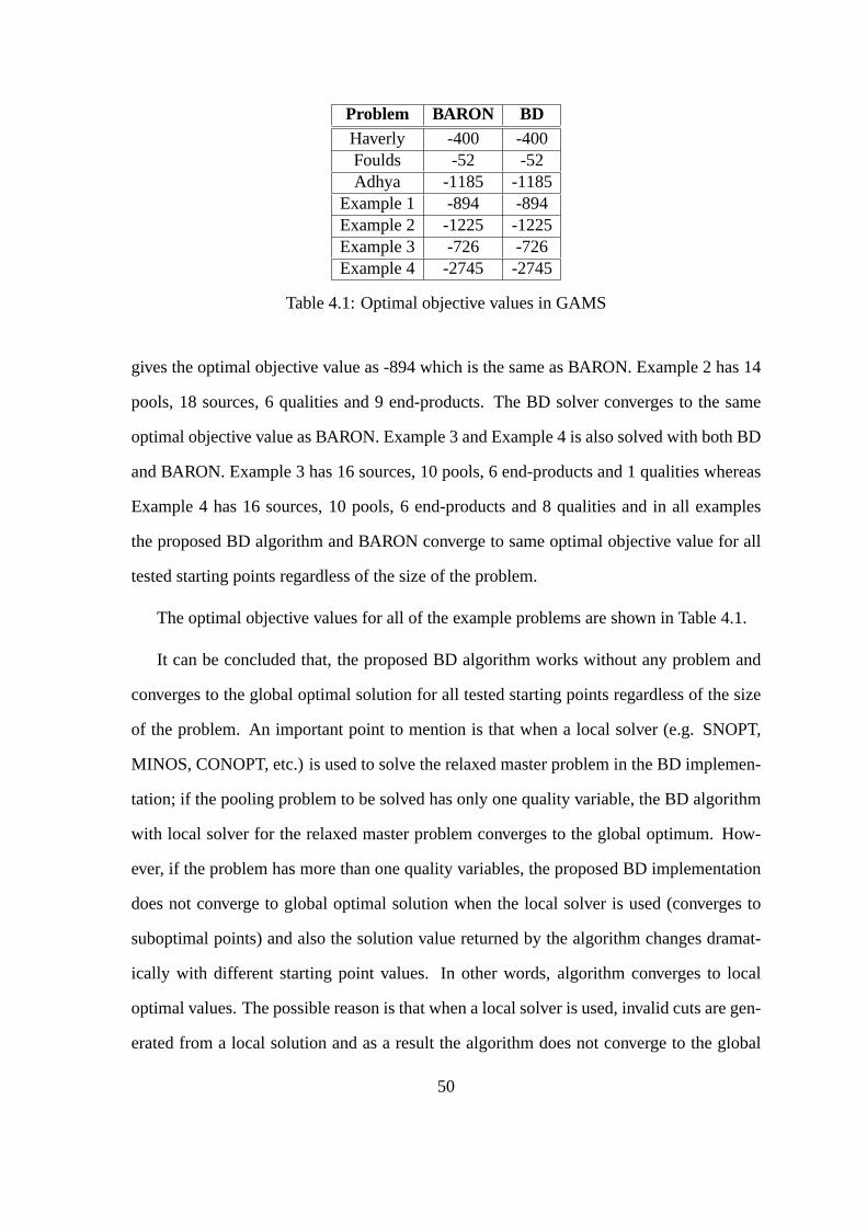
Problem BARON BDHaverly -400 -400Foulds -52 -52Adhya -1185 -1185
Example 1 -894 -894Example 2 -1225 -1225Example 3 -726 -726Example 4 -2745 -2745
Table 4.1: Optimal objective values in GAMS
gives the optimal objective value as -894 which is the same asBARON. Example 2 has 14
pools, 18 sources, 6 qualities and 9 end-products. The BD solver converges to the same
optimal objective value as BARON. Example 3 and Example 4 is also solved with both BD
and BARON. Example 3 has 16 sources, 10 pools, 6 end-productsand 1 qualities whereas
Example 4 has 16 sources, 10 pools, 6 end-products and 8 qualities and in all examples
the proposed BD algorithm and BARON converge to same optimal objective value for all
tested starting points regardless of the size of the problem.
The optimal objective values for all of the example problemsare shown in Table 4.1.
It can be concluded that, the proposed BD algorithm works without any problem and
converges to the global optimal solution for all tested starting points regardless of the size
of the problem. An important point to mention is that when a local solver (e.g. SNOPT,
MINOS, CONOPT, etc.) is used to solve the relaxed master problem in the BD implemen-
tation; if the pooling problem to be solved has only one quality variable, the BD algorithm
with local solver for the relaxed master problem converges to the global optimum. How-
ever, if the problem has more than one quality variables, theproposed BD implementation
does not converge to global optimal solution when the local solver is used (converges to
suboptimal points) and also the solution value returned by the algorithm changes dramat-
ically with different starting point values. In other words, algorithm converges to local
optimal values. The possible reason is that when a local solver is used, invalid cuts are gen-
erated from a local solution and as a result the algorithm does not converge to the global
50
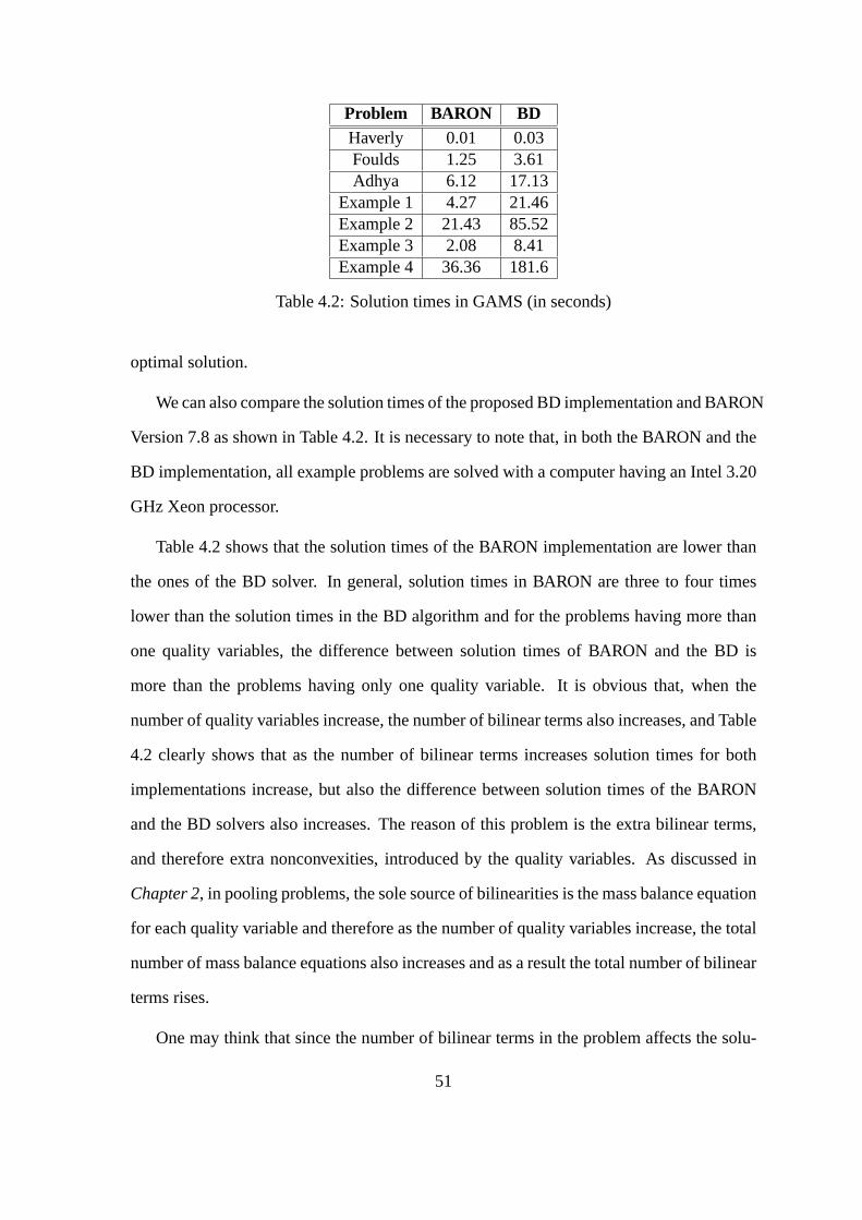
Problem BARON BDHaverly 0.01 0.03Foulds 1.25 3.61Adhya 6.12 17.13
Example 1 4.27 21.46Example 2 21.43 85.52Example 3 2.08 8.41Example 4 36.36 181.6
Table 4.2: Solution times in GAMS (in seconds)
optimal solution.
We can also compare the solution times of the proposed BD implementation and BARON
Version 7.8 as shown in Table 4.2. It is necessary to note that, in both the BARON and the
BD implementation, all example problems are solved with a computer having an Intel 3.20
GHz Xeon processor.
Table 4.2 shows that the solution times of the BARON implementation are lower than
the ones of the BD solver. In general, solution times in BARON are three to four times
lower than the solution times in the BD algorithm and for the problems having more than
one quality variables, the difference between solution times of BARON and the BD is
more than the problems having only one quality variable. It is obvious that, when the
number of quality variables increase, the number of bilinear terms also increases, and Table
4.2 clearly shows that as the number of bilinear terms increases solution times for both
implementations increase, but also the difference betweensolution times of the BARON
and the BD solvers also increases. The reason of this problem is the extra bilinear terms,
and therefore extra nonconvexities, introduced by the quality variables. As discussed in
Chapter 2, in pooling problems, the sole source of bilinearities is the mass balance equation
for each quality variable and therefore as the number of quality variables increase, the total
number of mass balance equations also increases and as a result the total number of bilinear
terms rises.
One may think that since the number of bilinear terms in the problem affects the solu-
51
tion times of the proposed BD solver drastically, this proposed BD algorithm can be useful
to solve problems with smaller number of bilinear terms suchas the gas network problems.
The gas network problems are a special kind of pooling problems where pools can be mod-
eled as mixers and splitters. Modeling pools as mixers and splitters gives the opportunity
to write mass balances for each quality separately.
For mixers, mass balances can be written as the sum of each flowregardless of the qual-
ity variables, therefore mass balance equations for mixersdo not include any bilinear terms.
In other words, for a selected quality, mass balance can be written as the output volume flow
rate equals to the sums of input volume flow rates and it is a linear equation. However, for
splitters, writing mass balances separately still introduces bilinear terms. However, now
since bilinear terms are only coming from the splitters instead of all of the pools, the num-
ber of bilinear terms reduces and therefore the complexity of the problem reduces greatly.
Thus, one can expect lower solution times from the BD solver ingas network problems. In
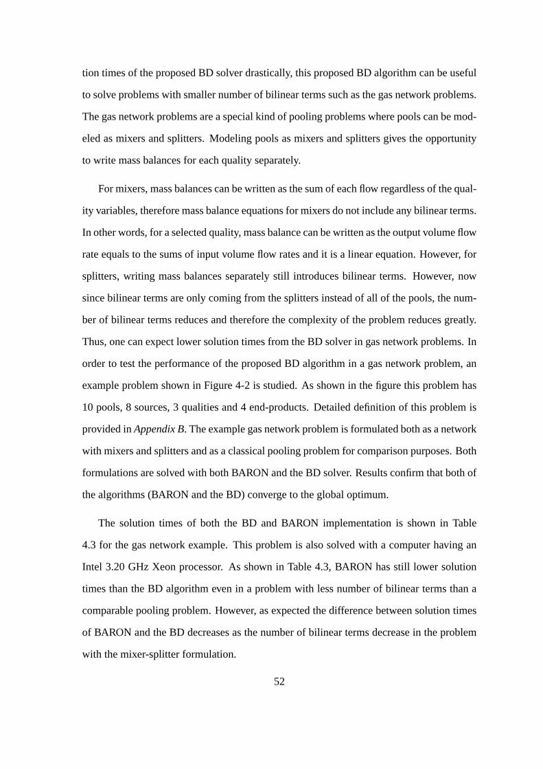
order to test the performance of the proposed BD algorithm in agas network problem, an
example problem shown in Figure 4-2 is studied. As shown in the figure this problem has
10 pools, 8 sources, 3 qualities and 4 end-products. Detailed definition of this problem is
provided inAppendix B. The example gas network problem is formulated both as a network
with mixers and splitters and as a classical pooling problemfor comparison purposes. Both
formulations are solved with both BARON and the BD solver. Results confirm that both of
the algorithms (BARON and the BD) converge to the global optimum.
The solution times of both the BD and BARON implementation is shown in Table
4.3 for the gas network example. This problem is also solved with a computer having an
Intel 3.20 GHz Xeon processor. As shown in Table 4.3, BARON has still lower solution
times than the BD algorithm even in a problem with less number of bilinear terms than a
comparable pooling problem. However, as expected the difference between solution times
of BARON and the BD decreases as the number of bilinear terms decrease in the problem
with the mixer-splitter formulation.
52

Figure 4-2: The gas network example
Formulation BARON BDGas Network 11.28 38.63
Pooling 13.72 42.91
Table 4.3: Solution times for the gas network problem (in seconds)
It can be seen from Table 4.3, solution times with BARON are lower than the ones
with the proposed BD solver in both formulations. However, animportant point to mention
is the decrease in the solution times of the BD algorithm with two different formulations
which confirms the expectations. This example clearly showsthat the performance of the
BD algorithm depends on the number of bilinear terms. In otherwords, as it is realized
in Table 4.2, as the number of bilinear terms increases in theproblem, the solution time
difference between BARON and the BD algorithm increases, because as the problem com-
plexity increases the number of iterations required by the BDsolver to converge to the
global optimal point increases.
However, when the output and log files of the problems solved in GAMS are inspected,
another important problem affecting the performance of theBD implementation is ob-
served. Since in the BD implementation, to iterate between the primal and master problem,
there is a loop and in every iteration for both primal and master problem GAMS executes
53

compilation and problem generation phases, in other words,in every iteration GAMS ex-
ecutes 2 compilations and 2 problem generations, and considering that the BD algorithm
iterates around 5-6 times to solve an average pooling problem, it incurs a total 10 to 12 com-
pilations and problem generations. In addition, in each iteration we should call BARON
to solve the relaxed master problem globally, these calls also cause executions of compi-
lations and problem generations in GAMS. Moreover, when thenumber of bilinear terms
increase, the number of iterations of the BD algoritm also increases and as a result the
number of compilations, problem generations and the numberof BARON calls to solve the
relaxed master problem in each iteration increases. However, BARON does both compila-
tion and problem generation only once in GAMS. This fact can explain the huge differences
in terms of the solution times between BARON and the BD algorithm when the number of
quality variables increase. Therefore, it is obvious that the proposed BD algorithm which
uses BARON at each iteration cannot compete against BARON inthe sense of solution
times. However, CPU times of the BD can still be considered close to BARON’s solution
times and it is quite reasonable to assume that by preventingthe executions of compilations
and problem generations in each iteration (i.e. changing the implementation such that the
problem generation and compilation occurs only once in the beginning of the execution)
plus with some tweak in the code, it is possible to get lower solution times from the BD
algorithm.
4.3.2 C++ Implementation
Since, GAMS executes compilation and problem generation ineach iteration and there is no
way to prevent these executions in GAMS; it is decided to reimplement the BD algorithm
by using C++. The algorithm is implemented in Linux and G++ (version 4.2) is used as the
compiler. As LP solver for the primal problem a subroutine that calls CPLEX 10.2 [21] as
the LP solver is used. However, the main issue is to write a custom B+B solver that can
handle the relaxed master problems. In GAMS, BARON is used tosolve bilinear relaxed
54
master problems, in C++ to solve them, there are two methods, one is to implement a B+B
code and the other one is to use the callable BARON library. The B+B solver implemented
is based on a B+B algorithm developed and implemented by Chaukun Lee in the Process
Systems Engineering Laboratory (PSEL) before.
However, BARON is a mature, commercially available and advanced software. There-
fore, a simple B+B code for the relaxed master problem cannot compete with it even if the
problem generation and compilation repetitions are omitted. There are two advantages of
BARON against a simple B+B algorithm. First one is the range (domain) reduction and
the second one is the tighter convex relaxations. Since range reduction has been presented
as the major feature of the branch and reduce algorithm, it isbelieved having more direct
effect in terms of solution times, therefore at first range reduction is applied.
Basically, range reduction is the process of eliminating regions from the feasible space
such that the removal does not affect the convergence of the algorithm to a global optimum.
Various techniques for range reduction have been proposed in the literature (Mangasar-
ian & McLiden (1985) [34], Thakur (1990) [46], Lamar (1993) [30], Savelsbergh (1994)
[43], Ryoo & Sahinidis (1996) [39], Shectman & Sahinidis (1998) [44] and Zamora &
Grossmann (1999) [51]), but in this study, in order to be as close to BARON’s methods as
possible, a range reduction algorithm proposed in Tawarmalani & Sahinidis (2002) [45] is
used.
Table 4.4 shows the effect of the implementation of the rangereduction. Although the
range reduction reduces the solution times almost half comparing to simple B+B algorithm,
it is still slower than BARON which shows that BARON has more weapons to reduce the
solution times and as mentioned one of them is the implementation of tighter convex relax-
ation techniques. The next step would be to implement the tighter relaxation techniques in
the literature to the BD algorithm but then it is decided to useBARON library instead for
convenience and to get quicker results.
In order to use all the advantages of BARON, a callable BARON library is obtained and
55
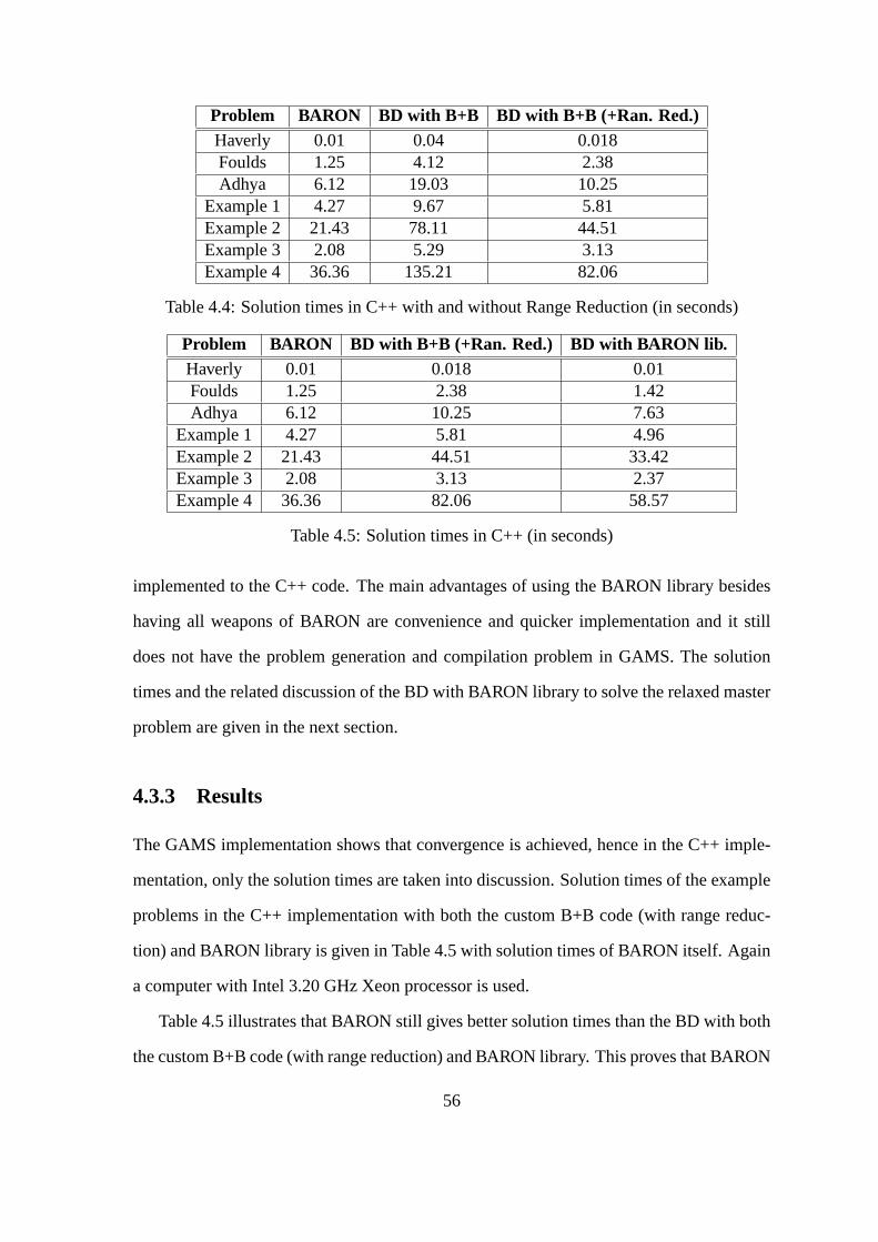
Problem BARON BD with B+B BD with B+B (+Ran. Red.)Haverly 0.01 0.04 0.018Foulds 1.25 4.12 2.38Adhya 6.12 19.03 10.25
Example 1 4.27 9.67 5.81Example 2 21.43 78.11 44.51Example 3 2.08 5.29 3.13Example 4 36.36 135.21 82.06
Table 4.4: Solution times in C++ with and without Range Reduction (in seconds)
Problem BARON BD with B+B (+Ran. Red.) BD with BARON lib.Haverly 0.01 0.018 0.01Foulds 1.25 2.38 1.42Adhya 6.12 10.25 7.63
Example 1 4.27 5.81 4.96Example 2 21.43 44.51 33.42Example 3 2.08 3.13 2.37Example 4 36.36 82.06 58.57
Table 4.5: Solution times in C++ (in seconds)
implemented to the C++ code. The main advantages of using the BARON library besides
having all weapons of BARON are convenience and quicker implementation and it still
does not have the problem generation and compilation problem in GAMS. The solution
times and the related discussion of the BD with BARON library to solve the relaxed master
problem are given in the next section.
4.3.3 Results
The GAMS implementation shows that convergence is achieved, hence in the C++ imple-
mentation, only the solution times are taken into discussion. Solution times of the example
problems in the C++ implementation with both the custom B+B code (with range reduc-
tion) and BARON library is given in Table 4.5 with solution times of BARON itself. Again
a computer with Intel 3.20 GHz Xeon processor is used.
Table 4.5 illustrates that BARON still gives better solution times than the BD with both
the custom B+B code (with range reduction) and BARON library.This proves that BARON
56

is a very powerful software to solve bilinear problems and even by using all the strategies
available, it is almost impossible to get better solution times with the BD algorithm. How-
ever, as mentioned in the first chapter, decomposition algorithms traditionally work more
efficiently than the B+B based algorithms in stochastic programming and the goal of this
study is to model the infrastructure development problem interms of gas quality variables
and therefore the results in deterministic pooling problems are not that important at this
stage. The real objective of this stage is to develop and implement a working BD algorithm
in order to use it to solve stochastic pooling problems. The reasons behind the author’s
expectations about the better efficiency of the BD in stochastic programming are explained
in the next chapter.
57

58
Chapter 5
Application to the Stochastic Pooling
Problem
5.1 Infrastructure Development Problems in Natural Gas
Value Chain
The prime objective is to solve long-term infrastructure development problems in the nat-
ural gas production industry considering all possible uncertainties and to develop new op-
timization methods, decision support tools for the infrastructure development problem.
Other research objectives are to develop methodology for analysis of robustness, flexi-
bility and risk in long-term infrastructure investments ingas production and to study how
operational flexibility should be incorporated in long terminvestments and infrastructure
analysis. In addition, it is necessary to demonstrate the methodology for analysis in impor-
tant industrial cases.
The complexity of the problem requires to develop new methodology and mathematical
models for the design, development and operation of infrastructure in natural gas produc-
tion under uncertainty and the main subsystems involved in the model will be the gas field,
the surface processing facilities, the transportation facilities and the markets.
59

The optimization model thus generated will be a large-scaleoptimization problem that
will involve a large number of nonconvex functions. Therefore, most probably this prob-
lem will be unsolvable by commercial solvers. Thus, better solution methods should be
explored to solve this problem to global optimality. Hence,it is possible that some theoret-
ical work will be required in optimization theory in the process of solving this problem.
Possible uncertainties in long-term infrastructure development problems in natural gas
production are production profiles and the amount of gas in natural gas fields; gas quality in
terms of heating value, NGL content, LPG content, CO2content etc. and the demands and
prices for the products of the gas value chain. Some important operational characteristics
of natural gas production networks such as blending and pooling possibilities, contractual
constraints, multiple routing and pipeline options and pressure constraints should also be
considered and incorporated into the production planning problem.
Then, it can be stated that there are three major research challenges that should be
addressed in the long-term infrastructure development problem: uncertainty and decision
flexibility; reaching global optimality of the overall system and combining economical
modeling with the production planning problem.
Uncertainty and decision flexibility is probably the most difficult challenge in a long
term production planning problem. Strategic decision support models for investment anal-
ysis need to capture the long term uncertainty and in addition be able to value short term
operational flexibility since the operational characteristics of initial investments, capacity
expansion and new investments will affect the decisions about the future investments and
capacity expansions.
Another important challenge is to reach optimality for the overall system. The timing
of investments, the inherent flexibility in technology choices and capacity decisions as
well as the location of the infrastructure are examples of decisions that should be analyzed
in a framework considering the overall system rather than a local subproblem to avoid
suboptimization.
60
The third research challenge is to incorporate economical modeling into the production
planning problem. In order to be able to capture both market driven production and opera-
tion, it is necessary to include the operational decision space of the infrastructure including
using markets to resolve bottlenecks of the infrastructureand dynamic market driven oper-
ation of the infrastructure. In addition, to capture the operational flexibility and limitations
of the system, it may be necessary to include detailed modelsof the technology.
In order to construct a mathematical model having all the properties of the value chain;
it is necessary to incorporate nonlinear flow and reservoir models, gas quality in the fields,
the contractual framework and LNG/LPG production models into the infrastructure devel-
opment problem with all possible uncertainties. Then, thisproblem becomes a large-scale
global optimization problem with stochasticity in it.
The first step chosen to start modeling the real value chain isto formulate a simple
model for the production planning problem for a relatively small field and integrate the
gas quality problem to this infrastructure development problem, since there are well known
algorithms to solve large pooling problems and then the possible next step is to solve this
problem at a larger-scale. Then, additional operational rules and uncertainties can be added
to this model in each step.
5.2 Introduction to Stochastic Programming
Stochastic programming is a framework for modeling optimization problems that involve
uncertainty. Whereas deterministic optimization problemsare formulated with known
parameters, real world problems almost invariably includesome unknown parameters.
Stochastic programming models take advantage of the fact that probability distributions
governing the data are known or can be estimated. The goal is to find some policy that is
feasible for all the possible data instances and maximizes the expectation of some function
of the decisions and the random variables. More generally, such models are formulated,
61
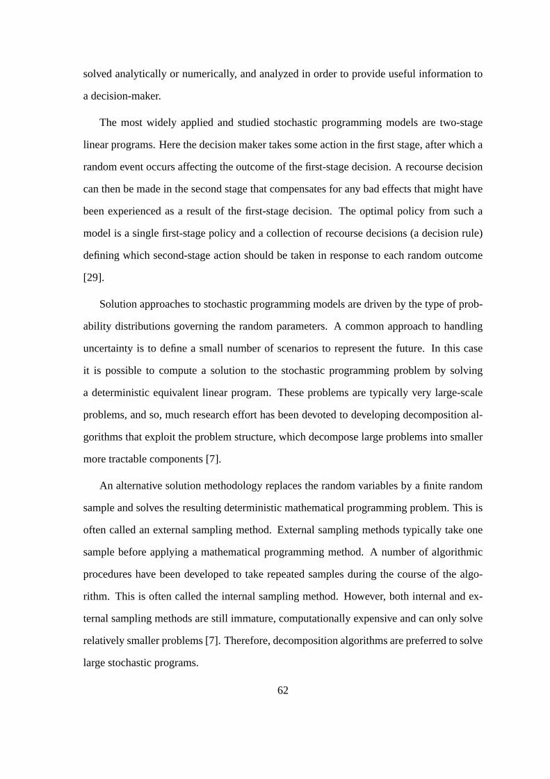
solved analytically or numerically, and analyzed in order to provide useful information to
a decision-maker.
The most widely applied and studied stochastic programmingmodels are two-stage
linear programs. Here the decision maker takes some action in the first stage, after which a
random event occurs affecting the outcome of the first-stagedecision. A recourse decision
can then be made in the second stage that compensates for any bad effects that might have
been experienced as a result of the first-stage decision. Theoptimal policy from such a
model is a single first-stage policy and a collection of recourse decisions (a decision rule)
defining which second-stage action should be taken in response to each random outcome
[29].
Solution approaches to stochastic programming models are driven by the type of prob-
ability distributions governing the random parameters. A common approach to handling
uncertainty is to define a small number of scenarios to represent the future. In this case
it is possible to compute a solution to the stochastic programming problem by solving
a deterministic equivalent linear program. These problemsare typically very large-scale
problems, and so, much research effort has been devoted to developing decomposition al-
gorithms that exploit the problem structure, which decompose large problems into smaller
more tractable components [7].
An alternative solution methodology replaces the random variables by a finite random
sample and solves the resulting deterministic mathematical programming problem. This is
often called an external sampling method. External sampling methods typically take one
sample before applying a mathematical programming method.A number of algorithmic
procedures have been developed to take repeated samples during the course of the algo-
rithm. This is often called the internal sampling method. However, both internal and ex-
ternal sampling methods are still immature, computationally expensive and can only solve
relatively smaller problems [7]. Therefore, decomposition algorithms are preferred to solve
large stochastic programs.
62

The basic idea behind decomposition algorithms is to decompose complex algorithms
into smaller parts and try to use the fact that solving many simpler programs may be quicker
than solving one large program. These algorithms are effective especially when the sub-
problems are easy to solve. Basically, decomposition algorithms works as shown in Figure
5-1. Each node in the figure represents a subproblem and the algorithm solves each sub-
problem separately and the solutions of parent nodes (represented asxt in the figure and
there is only one parent node in two-stage stochastic programs) are passed to child nodes
and the solutions of child nodes (represented asQt+1in the figure and there is only one stage
of child nodes in two-stage stochastic programs) are passedto parent nodes and both solu-
tions are updated until they converge. One important point to mention is that the solution
of child nodes have to be functions of the solutions of parentnodes since decisions in the
previous stage always determine the outcome of the problem in the following stage. How-
ever, in most of the stochastic problem formulations, the solutions of parent nodes are also
functions of the solutions of child nodes (For instance, second-stage operational variables
effecting the planning problem in the first stage in infrastructure development problems.).
Detailed information about the formulation of two-stage stochastic programs and solution
techniques can be found in Birge & Louveaux (1994) [7] and Kall& Wallace (1994) [29].
5.3 Importance of Stochastic Pooling Problems in Natural
Gas Infrastructure Development
Natural gas exploration and production is a highly capital-intensive industry. Facilities re-
quired for offshore exploration and production often remain in operation over the entire
life-span of the project, typically 10-30 years and hence the operational use of infrastruc-
ture and the requirements for its design change over time. Therefore, decisions regarding
investment in these facilities affect the profitability of the entire project. Given the large
potential profits and high investments in each project, there is significant interest in de-
63
Figure 5-1: Basic illustration of decomposition algorithmsin stochastic programming
veloping optimization models for planning in the natural gas exploration and production
industry. A major challenge lies in the fact that decision-makers in this industry have to
deal with a great deal of uncertainty. One of the most important sources of uncertainty is the
quality of reserves. The existence of oil or gas at a site is indicated by seismic surveys and
preliminary exploration tests. However, the actual amountof natural gas in these reserves,
and the efficacy of extracting these remain largely uncertain until after the investments have
been made. Both these factors directly affect the profitability of the project and hence it
is important to consider the impact of these uncertainties when formulating the decision
policy.
The opportunity for blending different sources of natural gas comes into the picture
especially when the natural gas upstream infrastructure isbeing developed. When new
wells or fields are being developed, it is possible to construct the pipeline system such that
the gas from different wells are mixed together to satisfy the requirements for different
qualities. However to construct the pipeline system optimally, a stochastic version of the
64
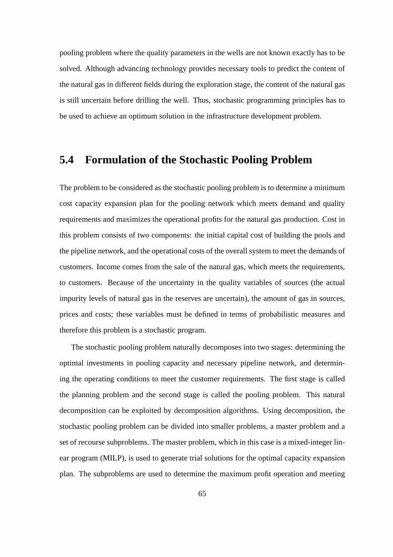
pooling problem where the quality parameters in the wells are not known exactly has to be
solved. Although advancing technology provides necessarytools to predict the content of
the natural gas in different fields during the exploration stage, the content of the natural gas
is still uncertain before drilling the well. Thus, stochastic programming principles has to
be used to achieve an optimum solution in the infrastructuredevelopment problem.
5.4 Formulation of the Stochastic Pooling Problem
The problem to be considered as the stochastic pooling problem is to determine a minimum
cost capacity expansion plan for the pooling network which meets demand and quality
requirements and maximizes the operational profits for the natural gas production. Cost in
this problem consists of two components: the initial capital cost of building the pools and
the pipeline network, and the operational costs of the overall system to meet the demands of
customers. Income comes from the sale of the natural gas, which meets the requirements,
to customers. Because of the uncertainty in the quality variables of sources (the actual
impurity levels of natural gas in the reserves are uncertain), the amount of gas in sources,
prices and costs; these variables must be defined in terms of probabilistic measures and
therefore this problem is a stochastic program.
The stochastic pooling problem naturally decomposes into two stages: determining the
optimal investments in pooling capacity and necessary pipeline network, and determin-
ing the operating conditions to meet the customer requirements. The first stage is called
the planning problem and the second stage is called the pooling problem. This natural
decomposition can be exploited by decomposition algorithms. Using decomposition, the
stochastic pooling problem can be divided into smaller problems, a master problem and a
set of recourse subproblems. The master problem, which in this case is a mixed-integer lin-
ear program (MILP), is used to generate trial solutions for the optimal capacity expansion
plan. The subproblems are used to determine the maximum profit operation and meeting
65

the requirements. Basically, subproblems are deterministic pooling problems (as formu-
lated inChapter 2) which are solved to maximize the profit after the optimal pooling net-
work is decided by the first stage capacity expansion problem. The planning problem has
originated from the long-term analysis of the electricity transmission and distribution with
price uncertainty. Basically, the planning problem is to make decisions about what to con-
struct, where to construct and how many (much) to construct.The pooling problem forms
the second stage. After the planning problem is solved at thefirst stage and the number of
pools and connections to and from them (into the sources and end-product nodes) are de-
cided by the solution of the planning problem; the pooling problem is solved as the second
stage and profit is maximized.
The stochastic pooling problem can be solved iteratively, by decomposition algorithms,
by alternately solving the master problem and the subproblems until an optimum is found.
In this way, the complex nonlinear program for stochastic pooling problem is reduced to
iterative solution of a MILP and a set of bilinear programs which reminds exactly the
methodology of the proposed BD algorithm to find global optimum. Therefore, the BD
algorithm can directly be used to solve stochastic pooling problems.
One of the most important issues in the stochastic version ofthe pooling problem is that
in the literature, proof of convergence for two-stage stochastic programs is only provided
for problems with a convex second stage. Unfortunately, thepooling problem is a noncon-
vex problem and hence the proofs from the literature cannot be applied directly to prove
the convergence of the stochastic pooling problem. However, the BD algorithm guarantees
to converge to global optimum in deterministic pooling problem and therefore, it is applied
to the stochastic version without any proof of convergence,but as a future work global
convergence for the BD algorithm in stochastic pooling problem has to be proved.
As explained, the first stage planning problem, which is an MILP, is to solve the optimal
capacity expansion plan and can be represented mathematically as follows:
66
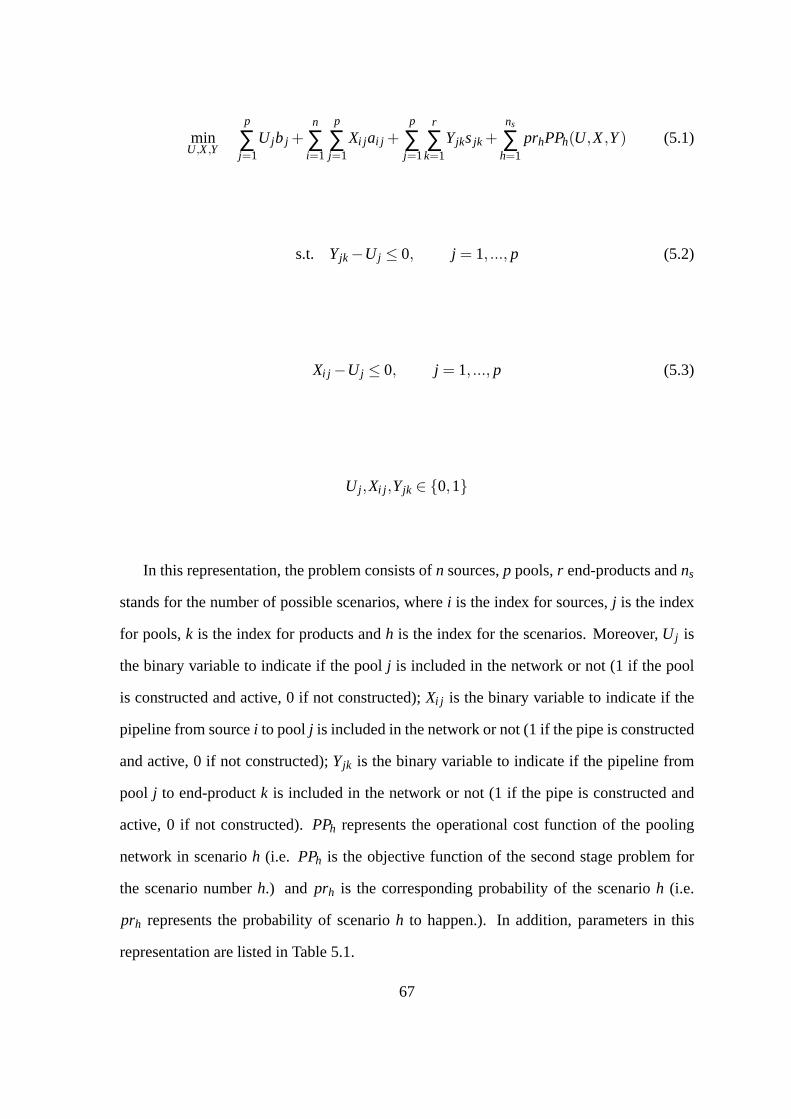
minU,X,Y
p
∑j=1
U jb j +n
∑i=1
p
∑j=1
Xi j ai j +p
∑j=1
r
∑k=1
Yjksjk +ns
∑h=1
prhPPh(U,X,Y) (5.1)
s.t. Yjk −U j ≤ 0, j = 1, ..., p (5.2)
Xi j −U j ≤ 0, j = 1, ..., p (5.3)
U j ,Xi j ,Yjk ∈ {0,1}
In this representation, the problem consists ofn sources,p pools,r end-products andns
stands for the number of possible scenarios, wherei is the index for sources,j is the index
for pools,k is the index for products andh is the index for the scenarios. Moreover,U j is
the binary variable to indicate if the poolj is included in the network or not (1 if the pool
is constructed and active, 0 if not constructed);Xi j is the binary variable to indicate if the
pipeline from sourcei to poolj is included in the network or not (1 if the pipe is constructed
and active, 0 if not constructed);Yjk is the binary variable to indicate if the pipeline from
pool j to end-productk is included in the network or not (1 if the pipe is constructedand
active, 0 if not constructed).PPh represents the operational cost function of the pooling
network in scenarioh (i.e. PPh is the objective function of the second stage problem for
the scenario numberh.) and prh is the corresponding probability of the scenarioh (i.e.
prh represents the probability of scenarioh to happen.). In addition, parameters in this
representation are listed in Table 5.1.
67
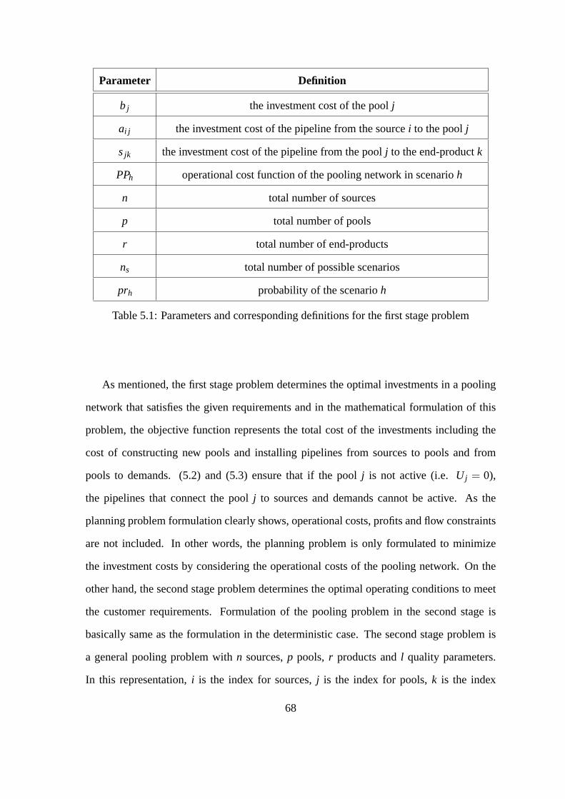
Parameter Definition
b j the investment cost of the poolj
ai j the investment cost of the pipeline from the sourcei to the poolj
sjk the investment cost of the pipeline from the poolj to the end-productk
PPh operational cost function of the pooling network in scenario h
n total number of sources
p total number of pools
r total number of end-products
ns total number of possible scenarios
prh probability of the scenarioh
Table 5.1: Parameters and corresponding definitions for thefirst stage problem
As mentioned, the first stage problem determines the optimalinvestments in a pooling
network that satisfies the given requirements and in the mathematical formulation of this
problem, the objective function represents the total cost of the investments including the
cost of constructing new pools and installing pipelines from sources to pools and from
pools to demands. (5.2) and (5.3) ensure that if the poolj is not active (i.e. U j = 0),
the pipelines that connect the poolj to sources and demands cannot be active. As the
planning problem formulation clearly shows, operational costs, profits and flow constraints
are not included. In other words, the planning problem is only formulated to minimize
the investment costs by considering the operational costs of the pooling network. On the
other hand, the second stage problem determines the optimaloperating conditions to meet
the customer requirements. Formulation of the pooling problem in the second stage is
basically same as the formulation in the deterministic case. The second stage problem is
a general pooling problem withn sources,p pools, r products andl quality parameters.
In this representation,i is the index for sources,j is the index for pools,k is the index
68
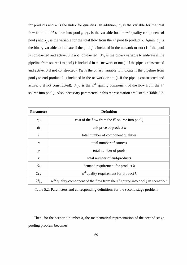
for products andw is the index for qualities. In addition,fi j is the variable for the total
flow from the ith source into poolj; q jw is the variable for thewth quality component of
pool j andx jk is the variable for the total flow from thejth pool to productk. Again,U j is
the binary variable to indicate if the poolj is included in the network or not (1 if the pool
is constructed and active, 0 if not constructed);Xi j is the binary variable to indicate if the
pipeline from sourcei to poolj is included in the network or not (1 if the pipe is constructed
and active, 0 if not constructed);Yjk is the binary variable to indicate if the pipeline from
pool j to end-productk is included in the network or not (1 if the pipe is constructedand
active, 0 if not constructed).λi jw is thewth quality component of the flow from theith
source into poolj. Also, necessary parameters in this representation are listed in Table 5.2.
Parameter Definition
ci j cost of the flow from theith source into poolj
dk unit price of productk
l total number of component qualities
n total number of sources
p total number of pools
r total number of end-products
Sk demand requirement for productk
Zkw wthquality requirement for productk
λ hi jw wth quality component of the flow from theith source into poolj in scenarioh
Table 5.2: Parameters and corresponding definitions for thesecond stage problem
Then, for the scenario numberh, the mathematical representation of the second stage
pooling problem becomes:
69

PPh(U,X,Y) = minf h,xh,qh
p
∑j=1
n
∑i=1
Xi j chi j f h
i j −r
∑k=1
dhk
p
∑j=1
Yjkxhjk (5.4)
s.t.n
∑i=1
Xi j f hi j −
r
∑k=1
Yjkxhjk = 0, j = 1, ..., p (5.5)
qhjw
r
∑k=1
Yjkxhjk −
n
∑i=1
λ hi jwXi j f h
i j = 0, j = 1, ..., p; w = 1, ..., l (5.6)
p
∑j=1
Yjkxhjk −Sk ≤ 0, k = 1, ..., r (5.7)
p
∑j=1
qhjwYjkxh
jk −Zkw
p
∑j=1
Yjkxhjk ≤ 0, k = 1, ..., r; w = 1, ..., l (5.8)
Xi j f Li j ≤ f h
i j ≤ Xi j fUi j , i = 1, ...,n j ; j = 1, ..., p
qLjw ≤ qh
jw ≤ qUjw, j = 1, ..., p; w = 1, ..., l
YjkxLjk ≤ xh
jk ≤YjkxUjk, j = 1, ..., p; k = 1, ..., r
In this formulation, the objective function represents thedifference between the cost
of the flow from the source nodes and the returns from selling the end-products. (5.5)
represents the mass balances for each active pool. (5.6) expresses the mass balance for
each quality component. (5.7) ensures that the flows to each end-product node do not
exceed the demands. (5.8) enforces that the quality requirements are satisfied at each end-
product node. Moreover, binary variables indicating whether the pipelines are active or not
(namely,Xi j andYjk) are added as multipliers to the lower and upper bounds of theflow
variables (into the pools and from the pools respectively) in order to to set flow variables to
70
zero in pipelines that do not exist.
In the stochastic pooling problem formulation, it is possible to set any combination of
the network parameters as the uncertain parameters (e.g. demand requirements for prod-
ucts, quality requirement for product, prices, costs or quality parameters at sources) after
excluding the known parameters which are provided or measured before formulating the
problem. Actually, in reality, all of the parameters in the pooling problem are uncertain
and hence this problem is a very difficult stochastic program. However, for convenience
and better understanding of the performance of the proposedBD algorithm, in all example
problems of this study, only the quality parameters of the flow from the sources into the
pools are taken as uncertain parameters and the remaining parameters are held constant for
all possible scenarios as explained in the next section. It is also important to mention here
the fact that the second stage problem in the stochastic pooling problem formulation is a
bilinear and hence nonconvex problem which makes this problem harder to solve.
5.5 Implementation of the BD Algorithm in Stochastic Pool-
ing Problems
With a finite number of scenarios, two-stage stochastic programs can be modeled as large
linear or nonlinear programming problems. This formulation is called the deterministic
equivalent. Strictly speaking a deterministic equivalentis any mathematical program that
can be used to compute the optimal first-stage decision, so these will exist for continuous
probability distributions as well, when one can represent the second-stage in some closed
form [29]. After formulating both stages, the stochastic pooling problem is reformulated to
a single stage (i.e. deterministic equivalent) by using thebasic conversion techniques which
are discussed in Birge & Louveaux (1994) [7] and Kall & Wallace(1994) [29] and the
resulting problem becomes a mixed-integer nonlinear program (MINLP). Since the second
stage optimization variables (namely,f , q andx) are not functions of uncertain parameters
71
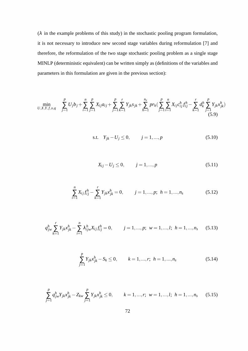
(λ in the example problems of this study) in the stochastic pooling program formulation,
it is not necessary to introduce new second stage variables during reformulation [7] and
therefore, the reformulation of the two stage stochastic pooling problem as a single stage
MINLP (deterministic equivalent) can be written simply as (definitions of the variables and
parameters in this formulation are given in the previous section):
minU,X,Y, f ,x,q
p
∑j=1
U jb j +n
∑i=1
p
∑j=1
Xi j ai j +p
∑j=1
r
∑k=1
Yjksjk +ns
∑h=1
prh(p
∑j=1
n
∑i=1
Xi j chi j f h
i j −r
∑k=1
dhk
p
∑j=1
Yjkxhjk)
(5.9)
s.t. Yjk −U j ≤ 0, j = 1, ..., p (5.10)
Xi j −U j ≤ 0, j = 1, ..., p (5.11)
n
∑i=1
Xi j f hi j −
r
∑k=1
Yjkxhjk = 0, j = 1, ..., p; h = 1, ...,ns (5.12)
qhjw
r
∑k=1
Yjkxhjk −
n
∑i=1
λ hi jwXi j f h
i j = 0, j = 1, ..., p; w = 1, ..., l ; h = 1, ...,ns (5.13)
p
∑j=1
Yjkxhjk −Sk ≤ 0, k = 1, ..., r; h = 1, ...,ns (5.14)
p
∑j=1
qhjwYjkxh
jk −Zkw
p
∑j=1
Yjkxhjk ≤ 0, k = 1, ..., r; w = 1, ..., l ; h = 1, ...,ns (5.15)
72
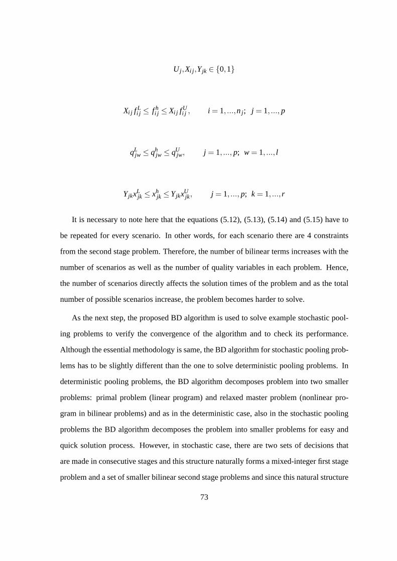
U j ,Xi j ,Yjk ∈ {0,1}
Xi j f Li j ≤ f h
i j ≤ Xi j fUi j , i = 1, ...,n j ; j = 1, ..., p
qLjw ≤ qh
jw ≤ qUjw, j = 1, ..., p; w = 1, ..., l
YjkxLjk ≤ xh
jk ≤YjkxUjk, j = 1, ..., p; k = 1, ..., r
It is necessary to note here that the equations (5.12), (5.13), (5.14) and (5.15) have to
be repeated for every scenario. In other words, for each scenario there are 4 constraints
from the second stage problem. Therefore, the number of bilinear terms increases with the
number of scenarios as well as the number of quality variables in each problem. Hence,
the number of scenarios directly affects the solution timesof the problem and as the total
number of possible scenarios increase, the problem becomesharder to solve.
As the next step, the proposed BD algorithm is used to solve example stochastic pool-
ing problems to verify the convergence of the algorithm and to check its performance.
Although the essential methodology is same, the BD algorithmfor stochastic pooling prob-
lems has to be slightly different than the one to solve deterministic pooling problems. In
deterministic pooling problems, the BD algorithm decomposes problem into two smaller
problems: primal problem (linear program) and relaxed master problem (nonlinear pro-
gram in bilinear problems) and as in the deterministic case,also in the stochastic pooling
problems the BD algorithm decomposes the problem into smaller problems for easy and
quick solution process. However, in stochastic case, thereare two sets of decisions that
are made in consecutive stages and this structure naturallyforms a mixed-integer first stage
problem and a set of smaller bilinear second stage problems and since this natural structure
73

of decomposition is different than the deterministic case,the proposed BD algorithm to
solve stochastic pooling problems has some changes from thedeterministic version. The
main difference between the stochastic and the deterministic versions is the process of
the formation of cuts in each iteration. In the deterministic version of the BD algorithm,
the additional cuts are generated for the bilinear relaxed master problem in each iteration;
however, in the stochastic version, the additional cuts aregenerated not for the bilinear
subproblems but for the MILP first stage problem.
Before explaining the BD algorithm for stochastic pooling problems in detail, first of
all, in order to be consistent with the stochastic programming literature, the first stage
optimal planning problem is called the master problem and the second stage optimal op-
erational problems are called the subproblems. The BD algorithm to solve the stochastic
version of this problem can be formulated as follows: A typical iteration starts with the
master problem without the additional cost coming from the subproblems (last summation
in 5.1). In other words, in the intial master problem, only first stage decision variables are
considered and the effect of the second stage variables to the first stage is neglected. The
binary vectors from solution of the master problem (U * , X* , Y* ) are fixed as the first stage
decision variables and subproblems for all scenarios are solved with these fixed decision
vectors. The objective function value of the master problemwith U * , X* andY* plus the
summation of the objective functions of each subproblem times its probability (as explained
in the problem formulation, a probability value is assignedto each scenario (subproblem).)
updates the upper bound (UBD) value, if it is lower than the previous UBD. Then additional
cuts are formed in the master problem by using the solutions of the subproblems and the
master problem are solved again with these additional cuts.The new solution of the master
problem provides new binary vectors (i.e.U * , X* andY* are updated after master prob-
lem is solved with additional cuts.). The objective function value of this updated master
problem updates the lower bound (LBD) value, if it is higher than the previous LBD. Then
the algorithm iterates and all of the subproblems are solvedagain with these new first stage
74
decision values and a new UBD (if necessary), plus additionalcuts for the master problem
are determined. The algorithm iterates until the lower bound value becomes higher than the
upper bound value. In other words, the solutions of the subproblems are used to find the
upper bound (UBD); the solution of the relaxed master problemis used to find the lower
bound (LBD). When LBD≥UBD, algorithm terminates. A detailed description of the BD
algorithm for stochastic pooling problems is provided in Algorithm 2.
A crucial point to note is that the subproblems in stochasticpooling problems are sim-
ply deterministic pooling problems (which are bilinear problems) since all binary first stage
decision variables are already fixed. Therefore, it is necessary to use a global solver to solve
the subproblems and since the proposed BD algorithm for the solution of the deterministic
pooling problems is shown to converge to global optimum, it is used to solve the sub-
problems in the stochastic pooling problems. In other words, in the implementation, the
proposed BD algorithm calls itself to solve the subproblems for every scenario. The rea-
son behind using the BD algorithm is the size of the stochasticpooling problems. Even the
largest deterministic pooling problem example solved in this study can be accepted as small
compared to the stochastic pooling problems since the stochastic ones have large number
of scenarios and each scenario itself is a large pooling problem and the BD algorithm has
advantages over any B+B based global optimization algorithmin large problems since it
decomposes very large problems into a number of smaller, more manageable problems in-
stead of solving it as a whole. Hence, the BD algorithm proposed for the deterministic
pooling problems is used as the solver for subproblems and itprovides both a background
for developing the BD algorithm for stochastic pooling problems and a tool to solve the
subproblems in the stochastic version of the BD algorithm.
Another important change in the implementation of the stochastic version of the algo-
rithm is the MILP solver since the LP solver (CPLEX [21]) in theBD implementation can
also be used as MILP solver with appropriate parameters. It is important to note that to
solve the subproblems, the BD implementation in C++ with the callable BARON library
75
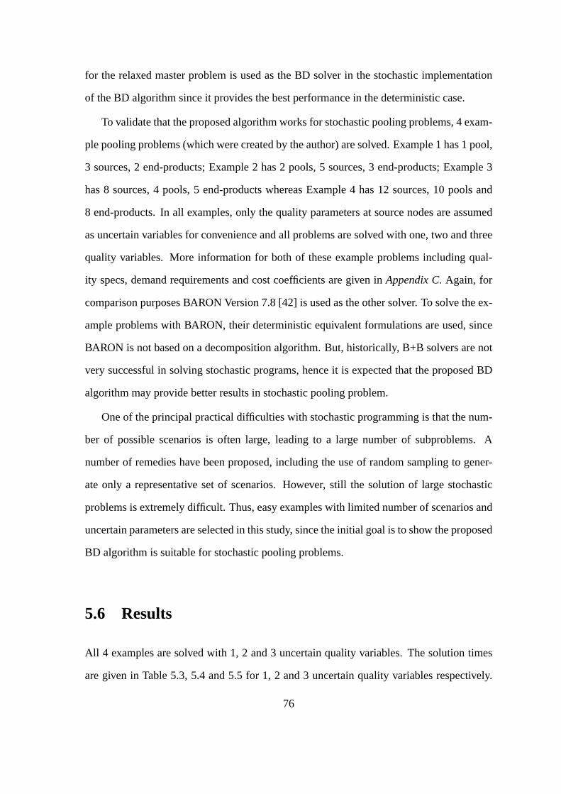
for the relaxed master problem is used as the BD solver in the stochastic implementation
of the BD algorithm since it provides the best performance in the deterministic case.
To validate that the proposed algorithm works for stochastic pooling problems, 4 exam-
ple pooling problems (which were created by the author) are solved. Example 1 has 1 pool,
3 sources, 2 end-products; Example 2 has 2 pools, 5 sources, 3end-products; Example 3
has 8 sources, 4 pools, 5 end-products whereas Example 4 has 12 sources, 10 pools and
8 end-products. In all examples, only the quality parameters at source nodes are assumed
as uncertain variables for convenience and all problems aresolved with one, two and three
quality variables. More information for both of these example problems including qual-
ity specs, demand requirements and cost coefficients are given inAppendix C. Again, for
comparison purposes BARON Version 7.8 [42] is used as the other solver. To solve the ex-
ample problems with BARON, their deterministic equivalentformulations are used, since
BARON is not based on a decomposition algorithm. But, historically, B+B solvers are not
very successful in solving stochastic programs, hence it isexpected that the proposed BD
algorithm may provide better results in stochastic poolingproblem.
One of the principal practical difficulties with stochasticprogramming is that the num-
ber of possible scenarios is often large, leading to a large number of subproblems. A
number of remedies have been proposed, including the use of random sampling to gener-
ate only a representative set of scenarios. However, still the solution of large stochastic
problems is extremely difficult. Thus, easy examples with limited number of scenarios and
uncertain parameters are selected in this study, since the initial goal is to show the proposed
BD algorithm is suitable for stochastic pooling problems.
5.6 Results
All 4 examples are solved with 1, 2 and 3 uncertain quality variables. The solution times
are given in Table 5.3, 5.4 and 5.5 for 1, 2 and 3 uncertain quality variables respectively.
76
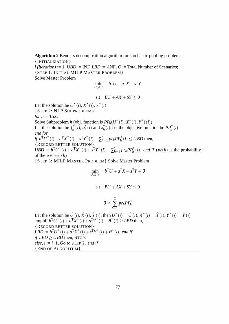
Algorithm 2 Benders decomposition algorithm for stochastic pooling problems{I NITIALIZATION }i (iteration) := 1, UBD := INF, LBD := -INF; C := Total Number of Scenarios;{STEP 1: INITIAL MILP M ASTER PROBLEM}Solve Master Problem
minU,X,Y
bTU +aTX +sTY
s.t BU +AX+SY≤ 0
Let the solution beU * (i), X* (i), Y* (i){STEP 2: NLP SUBPROBLEMS}for h = 1toCSolve Subproblemh (obj. function isPPh(U * (i) ,X* (i) ,Y* )(i))Let the solution bef *
h (i), q*h(i) andx*
h(i) Let the objective function bePP*h (i)
end forif bTU * (i)+aTX* (i)+sTY* (i)+∑C
h=1 prhPP*h (i) ≤UBD then,
{R ECORD BETTER SOLUTION}UBD := bTU * (i)+ aTX* (i)+ sTY* (i)+ ∑C
h=1 prhPP*h (i). end if (pr(h) is the probability
of the scenarioh){STEP 3: MILP MASTER PROBLEM} Solve Master Problem
minU,X,Y
bTU +aTX +sTY +θ
s.t BU +AX+SY≤ 0
θ ≥C
∑h=1
prhPP*h
Let the solution beU (i), X (i), Y (i), thenU * (i) = U (i), X* (i) = X (i), Y* (i) = Y (i)emphifbTU * (i)+aTX* (i)+sTY* (i)+θ * (i) ≥ LBD then,{R ECORD BETTER SOLUTION}LBD := bTU * (i)+aTX* (i)+sTY* (i)+θ * (i). end ifif LBD ≥UBD then, STOP.else, i:= i+1, Go toSTEP2. end if{E ND OF ALGORITHM}
77
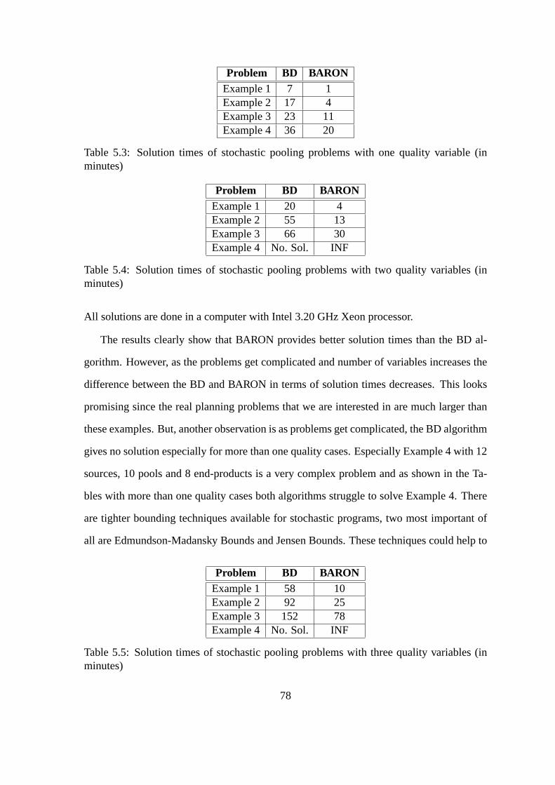
Problem BD BARONExample 1 7 1Example 2 17 4Example 3 23 11Example 4 36 20
Table 5.3: Solution times of stochastic pooling problems with one quality variable (inminutes)
Problem BD BARONExample 1 20 4Example 2 55 13Example 3 66 30Example 4 No. Sol. INF
Table 5.4: Solution times of stochastic pooling problems with two quality variables (inminutes)
All solutions are done in a computer with Intel 3.20 GHz Xeon processor.
The results clearly show that BARON provides better solution times than the BD al-
gorithm. However, as the problems get complicated and number of variables increases the
difference between the BD and BARON in terms of solution timesdecreases. This looks
promising since the real planning problems that we are interested in are much larger than
these examples. But, another observation is as problems get complicated, the BD algorithm
gives no solution especially for more than one quality cases. Especially Example 4 with 12
sources, 10 pools and 8 end-products is a very complex problem and as shown in the Ta-
bles with more than one quality cases both algorithms struggle to solve Example 4. There
are tighter bounding techniques available for stochastic programs, two most important of
all are Edmundson-Madansky Bounds and Jensen Bounds. These techniques could help to
Problem BD BARONExample 1 58 10Example 2 92 25Example 3 152 78Example 4 No. Sol. INF
Table 5.5: Solution times of stochastic pooling problems with three quality variables (inminutes)
78

reduce the solution times and solve larger problems with theBD algorithm, but, both of
them proved to provide tighter relaxations only for convex stochastic programs. Therefore,
in the next phase of the project, development of tighter relaxations for nonconvex stochas-
tic programs will be the objective. Author believes that a decomposition algorithm with
tighter bounds and an optimized code has still a better chance to solve stochastic problems
than a B+B algorithm.
Moreover, since all of these examples are not real cases and created by the author as
examples, it becomes difficult to create feasible examples as the problems get complicated.
Complex examples such as Example 4 has many parameters to be adjusted in order to
get a feasible problem and no one can guarantee the correctness of these parameters and
the feasibility of the problem. Infeasibilities occur during the analysis process and one
cannot determine whether these infeasibilities are results of incorrect parameters given by
the author or the formulation itself. Therefore, it is crucial to look for the methods to
generate feasible problems before proceeding further intothe bounding techniques. Hence,
as explained in the next chapter, the next step in this study will be to develop techniques to
generate feasible problems automatically.
79

80
Chapter 6
Conclusion
The prime objective of this project is to solve the long term infrastructure development
problem in the natural gas production industry with considering most of the possible un-
certainties and to develop new optimization methods, decision support tools for the infras-
tructure development problem. In addition, it is necessaryto demonstrate the methodology
for analysis in important industrial cases. The complexityof the problem requires to de-
velop new methodology and mathematical model for the design, development and opera-
tion of infrastructure in natural gas production under uncertainty and the main subsystems
involved in the model will be the gas field, the surface processing facilities, the transporta-
tion facilities and the markets.
This is a very difficult goal to achieve when considering the requirement of huge math-
ematical models to be as close as possible to reality. Therefore, it is decided to start from
relatively smaller problems by assuming most of the variables are known parameters and
try to deal with only one aspect of the whole value chain. Because of the reasons explained
above, the first stage in this project is chosen to be the planning problem only considering
the pooling and blending of the natural gas from different fields with uncertain quality vari-
ables. To solve even this relatively small model a new BD algorithm has to be proposed
because of the nonconvexity of the pooling problem.
81
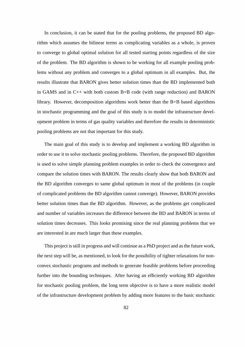
In conclusion, it can be stated that for the pooling problems, the proposed BD algo-
rithm which assumes the bilinear terms as complicating variables as a whole, is proven
to converge to global optimal solution for all tested starting points regardless of the size
of the problem. The BD algorithm is shown to be working for all example pooling prob-
lems without any problem and converges to a global optimum inall examples. But, the
results illustrate that BARON gives better solution times than the BD implemented both
in GAMS and in C++ with both custom B+B code (with range reduction) and BARON
library. However, decomposition algorithms work better than the B+B based algorithms
in stochastic programming and the goal of this study is to model the infrastructure devel-
opment problem in terms of gas quality variables and therefore the results in deterministic
pooling problems are not that important for this study.
The main goal of this study is to develop and implement a working BD algorithm in
order to use it to solve stochastic pooling problems. Therefore, the proposed BD algorithm
is used to solve simple planning problem examples in order tocheck the convergence and
compare the solution times with BARON. The results clearly show that both BARON and
the BD algorithm converges to same global optimum in most of the problems (in couple
of complicated problems the BD algorithm cannot converge). However, BARON provides
better solution times than the BD algorithm. However, as the problems get complicated
and number of variables increases the difference between the BD and BARON in terms of
solution times decreases. This looks promising since the real planning problems that we
are interested in are much larger than these examples.
This project is still in progress and will continue as a PhD project and as the future work,
the next step will be, as mentioned, to look for the possibility of tighter relaxations for non-
convex stochastic programs and methods to generate feasible problems before proceeding
further into the bounding techniques. After having an efficiently working BD algorithm
for stochastic pooling problem, the long term objective is to have a more realistic model
of the infrastructure development problem by adding more features to the basic stochastic
82

pooling problem step by step and develop the BD algorithm so itcan handle these large
scale stochastic programs.
83

84

Appendix A
Example Pooling Problems
To validate the algorithm and check its performance, 7 example pooling problems are
solved with both the proposed BD algorithm and BARON [42]. 3 ofthese example prob-
lems are taken directly from the literature (Haverly’s, Adhya’s and Fould’s pooling prob-
lems), the remaining 4 problems are created by the author to check the performance of the
algorithm in more complex pooling problems. In this chapter, detailed information is pre-
sented about these example problems including quality specs, demand requirements, cost
coefficients and GAMS implementations. Since Haverly’s pooling problem is formulated
in detail inChapter 2, this chapter excludes it and contains remaining 6 problems.
A.1 Adhya’s Pooling Problem
One of the example problems used is taken from Adhya et. al. (1999) [1]. In this problem,
the number of pools is 7, the number of sources is 8, the numberof qualities is 4 and the
number of end-products is 4. Necessary parameters (qualityparameters, costs, prices and
demand requirements) to construct this problem is given in Tables A.1, A.2, A.3, A.4 and
A.5. GAMS implementation of Adhya’s problem is also provided at the end of this Chapter.
85
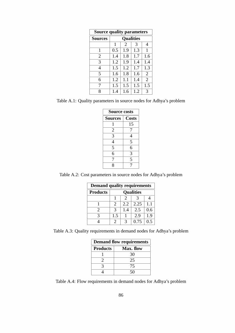
Source quality parametersSources Qualities
1 2 3 41 0.5 1.9 1.3 12 1.4 1.8 1.7 1.63 1.2 1.9 1.4 1.44 1.5 1.2 1.7 1.35 1.6 1.8 1.6 26 1.2 1.1 1.4 27 1.5 1.5 1.5 1.58 1.4 1.6 1.2 3
Table A.1: Quality parameters in source nodes for Adhya’s problem
Source costsSources Costs
1 152 73 44 55 66 37 58 7
Table A.2: Cost parameters in source nodes for Adhya’s problem
Demand quality requirementsProducts Qualities
1 2 3 41 2 2.2 2.25 1.12 3 1.4 2.5 0.63 1.5 1 2.9 1.94 2 3 0.75 0.5
Table A.3: Quality requirements in demand nodes for Adhya’sproblem
Demand flow requirementsProducts Max. flow
1 302 253 754 50
Table A.4: Flow requirements in demand nodes for Adhya’s problem
86
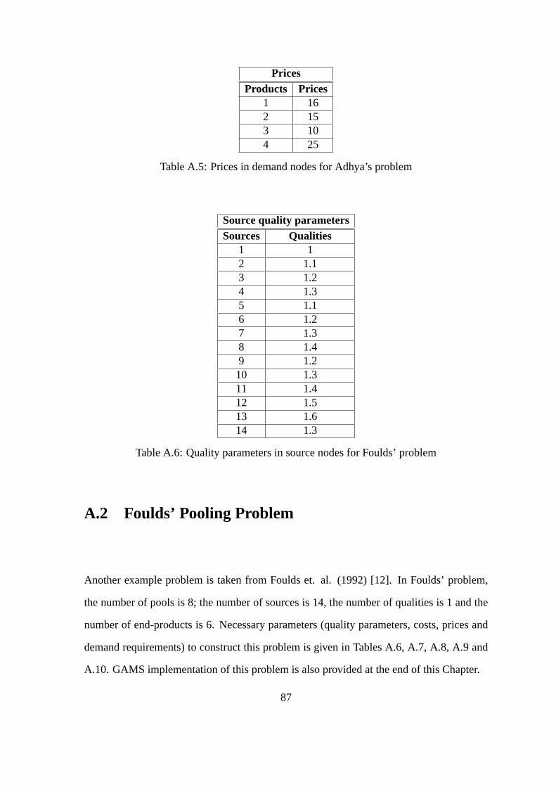
PricesProducts Prices
1 162 153 104 25
Table A.5: Prices in demand nodes for Adhya’s problem
Source quality parametersSources Qualities
1 12 1.13 1.24 1.35 1.16 1.27 1.38 1.49 1.210 1.311 1.412 1.513 1.614 1.3
Table A.6: Quality parameters in source nodes for Foulds’ problem
A.2 Foulds’ Pooling Problem
Another example problem is taken from Foulds et. al. (1992) [12]. In Foulds’ problem,
the number of pools is 8; the number of sources is 14, the number of qualities is 1 and the
number of end-products is 6. Necessary parameters (qualityparameters, costs, prices and
demand requirements) to construct this problem is given in Tables A.6, A.7, A.8, A.9 and
A.10. GAMS implementation of this problem is also provided at the end of this Chapter.
87
Source costsSources Costs
1 202 193 184 175 196 187 178 169 1810 1711 1612 1513 1714 16
Table A.7: Cost parameters in source nodes for Foulds’ problem
Demand quality requirementsProducts Qualities
1 1.052 1.13 1.154 1.25 1.256 1.3
Table A.8: Quality requirements in demand nodes for Foulds’problem
Demand flow requirementsProducts Max. flow
1 302 293 284 275 266 25
Table A.9: Flow requirements in demand nodes for Foulds’ problem
88

PricesProducts Prices
1 202 19.53 194 18.55 186 17.5
Table A.10: Prices in demand nodes for Foulds’ problem
A.3 Example 1
The first example problem (Example 1) has 14 pools, 18 sources, 1 quality and 9 end-
products. Necessary parameters (quality parameters, costs, prices and demand require-
ments) to construct this problem is given in Tables A.11, A.12, A.13, A.14 and A.15.
GAMS implementation of this problem is also provided at the end of this Chapter.
A.4 Example 2
The second example problem (Example 2) has 14 pools, 18 sources, 6 qualities and 9 end-
products. Necessary parameters (quality parameters, costs, prices and demand require-
ments) to construct this problem is given in Tables A.16, A.17, A.18, A.19 and A.20.
GAMS implementation of this problem is also provided at the end of this Chapter.
A.5 Example 3
The third example problem (Example 3) has 16 sources, 10 pools, 6 end-products and
1 quality variable. Necessary parameters (quality parameters, costs, prices and demand
requirements) to construct this problem is given in Tables A.21, A.22, A.23, A.24 and
A.25. GAMS implementation of this problem is also provided at the end of this Chapter.
89
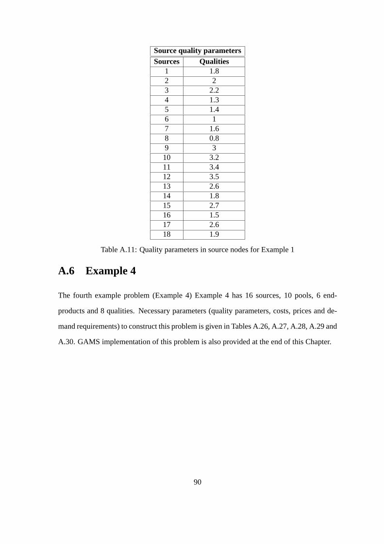
Source quality parametersSources Qualities
1 1.82 23 2.24 1.35 1.46 17 1.68 0.89 310 3.211 3.412 3.513 2.614 1.815 2.716 1.517 2.618 1.9
Table A.11: Quality parameters in source nodes for Example 1
A.6 Example 4
The fourth example problem (Example 4) Example 4 has 16 sources, 10 pools, 6 end-
products and 8 qualities. Necessary parameters (quality parameters, costs, prices and de-
mand requirements) to construct this problem is given in Tables A.26, A.27, A.28, A.29 and
A.30. GAMS implementation of this problem is also provided at the end of this Chapter.
90

Source costsSources Costs
1 102 53 64 85 136 257 168 189 3510 511 2012 1513 1114 2415 2016 2517 1018 14
Table A.12: Cost parameters in source nodes for Example 1
Demand quality requirementsProducts Qualities
1 32 2.13 1.54 1.25 2.66 2.57 18 1.759 3.2
Table A.13: Quality requirements in demand nodes for Example 1
91
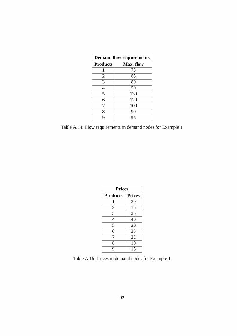
Demand flow requirementsProducts Max. flow
1 752 853 804 505 1306 1207 1008 909 95
Table A.14: Flow requirements in demand nodes for Example 1
PricesProducts Prices
1 302 153 254 405 306 357 228 109 15
Table A.15: Prices in demand nodes for Example 1
92

Source quality parametersSources Qualities
1 2 3 4 5 61 1.8 2.9 1.5 3 0.8 1.42 2.2 4.8 3.8 4.6 2.7 3.63 2 5 3 2.4 4 24 1.5 3.2 2.7 2.5 1.7 0.95 3.6 2.8 0.6 2 3.1 26 3.2 4.1 1.4 2.8 0.8 4.87 4 5 1.5 3.5 4.2 2.18 4.5 1.6 2.2 3.8 1.2 39 0.8 1.9 1.3 4 1.3 1.610 1.4 0.8 1.7 2.6 3.7 1.911 2.2 1.9 1.4 1 3.4 512 1.5 1 3.7 4.3 3.7 0.813 2.6 2.8 1.6 2.4 3.6 214 1.2 3.1 1.4 2.8 1 2.615 1.9 1.5 3.2 0.8 1.8 3.516 2.4 1.8 5 4 2.2 317 3.5 2.5 1.8 3.6 5 4.618 4.4 2.6 1.2 3 4.2 4
Table A.16: Quality parameters in source nodes for Example 2
93
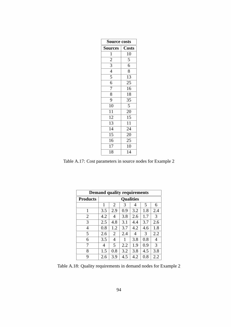
Source costsSources Costs
1 102 53 64 85 136 257 168 189 3510 511 2012 1513 1114 2415 2016 2517 1018 14
Table A.17: Cost parameters in source nodes for Example 2
Demand quality requirementsProducts Qualities
1 2 3 4 5 61 3.5 2.9 0.9 3.2 1.8 2.42 4.2 4 3.8 2.6 1.7 33 2.5 4.8 3.1 4.4 3.7 2.64 0.8 1.2 3.7 4.2 4.6 1.85 2.6 2 2.4 4 3 2.26 3.5 4 1 3.8 0.8 47 4 5 2.2 1.9 0.9 38 1.5 0.8 3.2 3.8 4.5 3.89 2.6 3.9 4.5 4.2 0.8 2.2
Table A.18: Quality requirements in demand nodes for Example 2
94

Demand flow requirementsProducts Max. flow
1 752 853 804 505 1306 1207 1008 909 95
Table A.19: Flow requirements in demand nodes for Example 2
PricesProducts Prices
1 302 153 254 405 306 357 228 109 15
Table A.20: Prices in demand nodes for Example 2
95
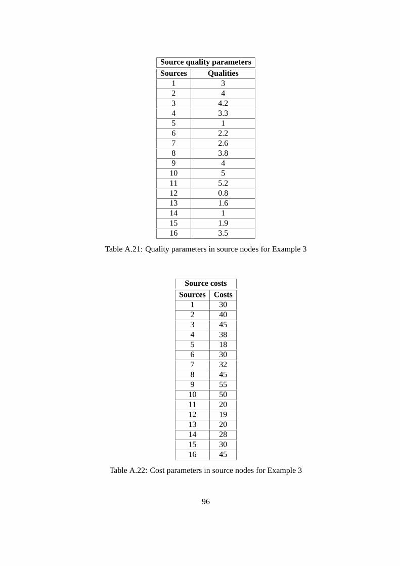
Source quality parametersSources Qualities
1 32 43 4.24 3.35 16 2.27 2.68 3.89 410 511 5.212 0.813 1.614 115 1.916 3.5
Table A.21: Quality parameters in source nodes for Example 3
Source costsSources Costs
1 302 403 454 385 186 307 328 459 5510 5011 2012 1913 2014 2815 3016 45
Table A.22: Cost parameters in source nodes for Example 3
96
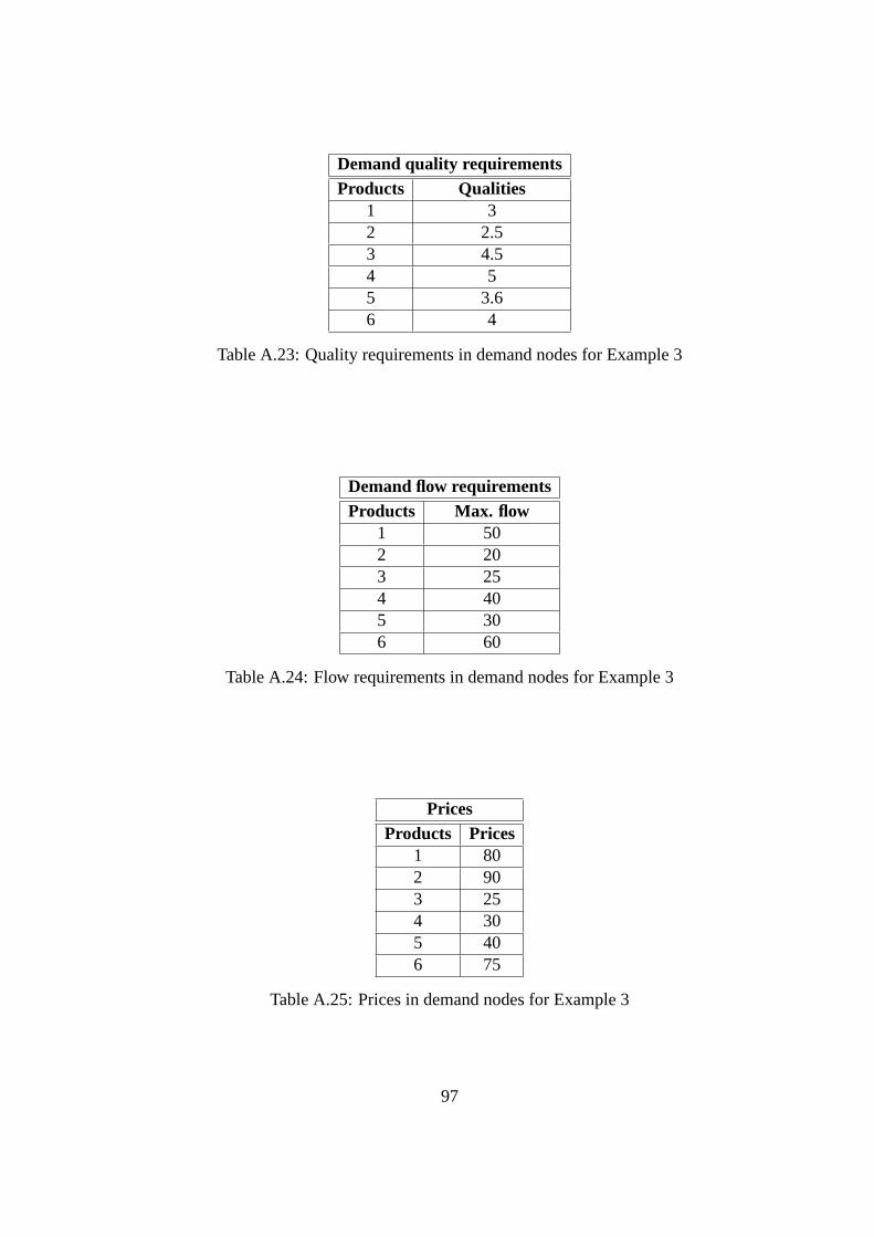
Demand quality requirementsProducts Qualities
1 32 2.53 4.54 55 3.66 4
Table A.23: Quality requirements in demand nodes for Example 3
Demand flow requirementsProducts Max. flow
1 502 203 254 405 306 60
Table A.24: Flow requirements in demand nodes for Example 3
PricesProducts Prices
1 802 903 254 305 406 75
Table A.25: Prices in demand nodes for Example 3
97

Source quality parametersSources Qualities
1 2 3 4 5 6 7 81 4 4.5 5 3.1 0.8 1.4 2.8 4.12 3.2 3.8 1 4 2.2 4.6 3 1.63 2.5 5.6 2.6 2.9 4 5 2 14 3.2 5.2 4.7 2 1.5 4 0.8 55 3 1.8 0.2 2 3.5 3 4.2 1.96 3.8 4 6 2.8 4.5 5.8 3.4 4.67 4 5.2 4.5 3.5 2 2 2.8 18 4.5 2.6 5.2 3.8 6.2 2.3 0.5 1.59 4.8 0.8 0.3 4 1.9 0.6 0.9 410 1 3.1 2 2.6 0.7 1 5 1.211 2.8 1 4.4 1 5.4 5.1 4 112 1.5 4.1 4.7 5.3 3.7 1 1.8 0.613 0.6 3 5.8 1.4 3.6 0.2 2 2.514 1.6 3.8 0.9 3.8 1 0.6 3 515 3.9 4.5 4.2 4 1.8 5.5 1.2 4.616 4.4 4.8 5.2 2.9 4.2 4.5 1.5 3.1
Table A.26: Quality parameters in source nodes for Example 4
Source costsSources Costs
1 302 403 454 385 186 307 328 459 5510 5011 2012 1913 2014 2815 3016 45
Table A.27: Cost parameters in source nodes for Example 4
98
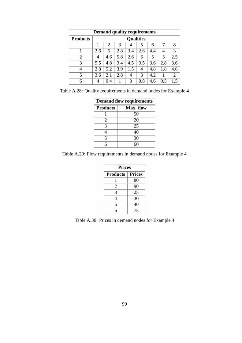
Demand quality requirementsProducts Qualities
1 2 3 4 5 6 7 81 3.6 5 2.8 3.4 2.6 4.4 4 32 4 4.6 5.8 2.6 6 5 5 2.53 5.5 4.8 3.4 4.5 3.5 3.6 2.8 3.64 2.8 5.2 3.9 1.5 4 4.8 1.8 4.65 3.6 2.1 2.8 4 3 4.2 1 26 4 0.4 1 3 0.8 4.6 0.5 1.5
Table A.28: Quality requirements in demand nodes for Example 4
Demand flow requirementsProducts Max. flow
1 502 203 254 405 306 60
Table A.29: Flow requirements in demand nodes for Example 4
PricesProducts Prices
1 802 903 254 305 406 75
Table A.30: Prices in demand nodes for Example 4
99
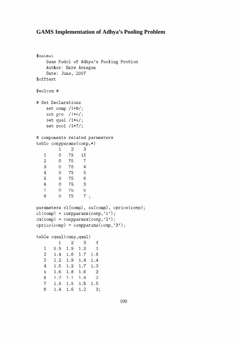
GAMS Implementation of Adhya’s Pooling Problem
$ontext
Gams Model of Adhya's Pooling Problem
Author: Emre Armagan
Date: June, 2007
$offtext
$eol om #
# Set De larations
set omp /1*8/;
set pro /1*4/;
set qual /1*4/;
set pool /1*7/;
# omponents related parameters
table ompparams( omp,*)
1 2 3
1 0 75 15
2 0 75 7
3 0 75 4
4 0 75 5
5 0 75 6
6 0 75 3
7 0 75 5
8 0 75 7 ;
parameters l( omp), u( omp), pri e( omp);
l( omp) = ompparams( omp,'1');
u( omp) = ompparams( omp,'2');
pri e( omp) = ompparams( omp,'3');
table qual( omp,qual)
1 2 3 4
1 0.5 1.9 1.3 1
2 1.4 1.8 1.7 1.6
3 1.2 1.9 1.4 1.4
4 1.5 1.2 1.7 1.3
5 1.6 1.8 1.6 2
6 1.2 1.1 1.4 2
7 1.5 1.5 1.5 1.5
8 1.4 1.6 1.2 3;
100
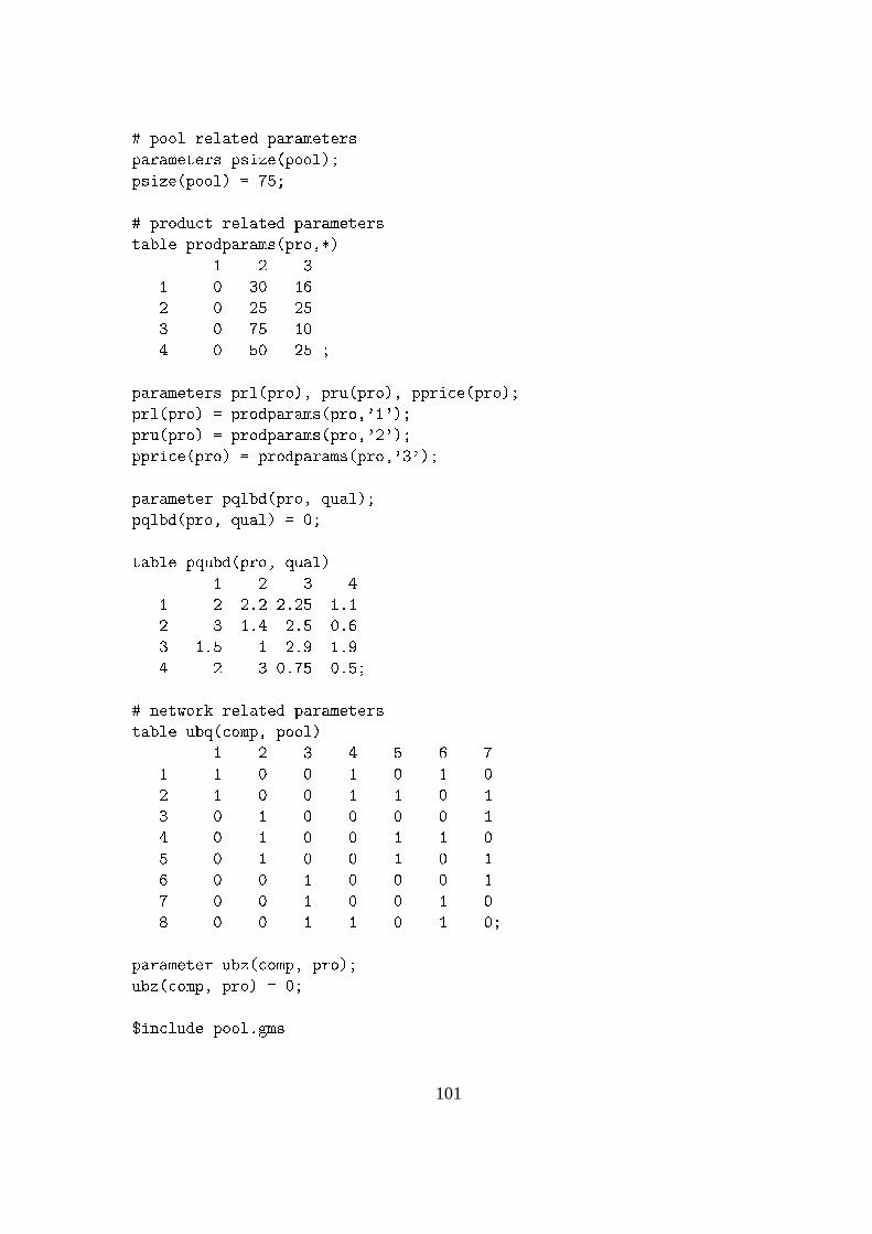
# pool related parameters
parameters psize(pool);
psize(pool) = 75;
# produ t related parameters
table prodparams(pro,*)
1 2 3
1 0 30 16
2 0 25 25
3 0 75 10
4 0 50 25 ;
parameters prl(pro), pru(pro), ppri e(pro);
prl(pro) = prodparams(pro,'1');
pru(pro) = prodparams(pro,'2');
ppri e(pro) = prodparams(pro,'3');
parameter pqlbd(pro, qual);
pqlbd(pro, qual) = 0;
table pqubd(pro, qual)
1 2 3 4
1 2 2.2 2.25 1.1
2 3 1.4 2.5 0.6
3 1.5 1 2.9 1.9
4 2 3 0.75 0.5;
# network related parameters
table ubq( omp, pool)
1 2 3 4 5 6 7
1 1 0 0 1 0 1 0
2 1 0 0 1 1 0 1
3 0 1 0 0 0 0 1
4 0 1 0 0 1 1 0
5 0 1 0 0 1 0 1
6 0 0 1 0 0 0 1
7 0 0 1 0 0 1 0
8 0 0 1 1 0 1 0;
parameter ubz( omp, pro);
ubz( omp, pro) = 0;
$in lude pool.gms
101
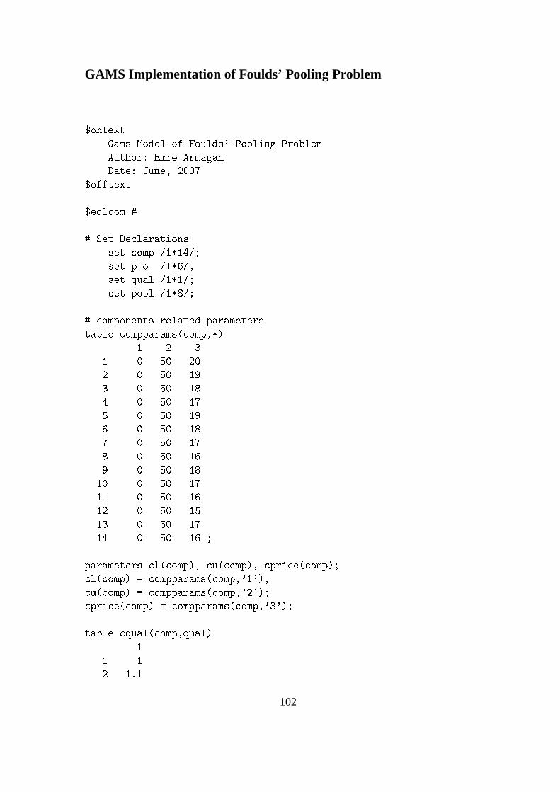
GAMS Implementation of Foulds’ Pooling Problem
$ontext
Gams Model of Foulds' Pooling Problem
Author: Emre Armagan
Date: June, 2007
$offtext
$eol om #
# Set De larations
set omp /1*14/;
set pro /1*6/;
set qual /1*1/;
set pool /1*8/;
# omponents related parameters
table ompparams( omp,*)
1 2 3
1 0 50 20
2 0 50 19
3 0 50 18
4 0 50 17
5 0 50 19
6 0 50 18
7 0 50 17
8 0 50 16
9 0 50 18
10 0 50 17
11 0 50 16
12 0 50 15
13 0 50 17
14 0 50 16 ;
parameters l( omp), u( omp), pri e( omp);
l( omp) = ompparams( omp,'1');
u( omp) = ompparams( omp,'2');
pri e( omp) = ompparams( omp,'3');
table qual( omp,qual)
1
1 1
2 1.1
102
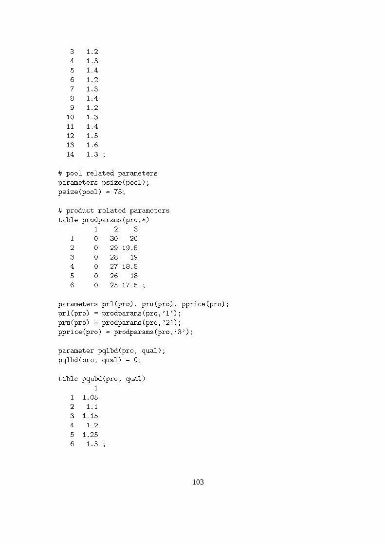
3 1.2
4 1.3
5 1.4
6 1.2
7 1.3
8 1.4
9 1.2
10 1.3
11 1.4
12 1.5
13 1.6
14 1.3 ;
# pool related parameters
parameters psize(pool);
psize(pool) = 75;
# produ t related parameters
table prodparams(pro,*)
1 2 3
1 0 30 20
2 0 29 19.5
3 0 28 19
4 0 27 18.5
5 0 26 18
6 0 25 17.5 ;
parameters prl(pro), pru(pro), ppri e(pro);
prl(pro) = prodparams(pro,'1');
pru(pro) = prodparams(pro,'2');
ppri e(pro) = prodparams(pro,'3');
parameter pqlbd(pro, qual);
pqlbd(pro, qual) = 0;
table pqubd(pro, qual)
1
1 1.05
2 1.1
3 1.15
4 1.2
5 1.25
6 1.3 ;
103
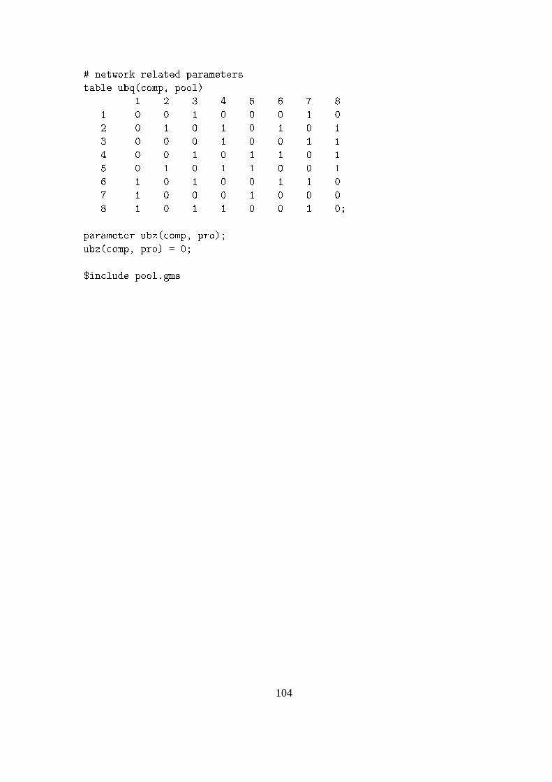
# network related parameters
table ubq( omp, pool)
1 2 3 4 5 6 7 8
1 0 0 1 0 0 0 1 0
2 0 1 0 1 0 1 0 1
3 0 0 0 1 0 0 1 1
4 0 0 1 0 1 1 0 1
5 0 1 0 1 1 0 0 1
6 1 0 1 0 0 1 1 0
7 1 0 0 0 1 0 0 0
8 1 0 1 1 0 0 1 0;
parameter ubz( omp, pro);
ubz( omp, pro) = 0;
$in lude pool.gms
104

GAMS Implementation of Example 1
$ontext
Gams Model of Example 1 Pooling Problem
Author: Emre Armagan
Date: July, 2007
$offtext
$eol om #
# Set De larations
set omp /1*18/;
set pro /1*9/;
set qual /1*1/;
set pool /1*14/;
# omponents related parameters
table ompparams( omp,*)
1 2 3
1 0 200 10
2 0 200 5
3 0 200 6
4 0 200 8
5 0 200 13
6 0 200 25
7 0 200 16
8 0 200 18
9 0 200 35
10 0 200 5
11 0 200 20
12 0 200 15
13 0 200 11
14 0 200 24
15 0 200 20
16 0 200 25
17 0 200 10
18 0 200 14 ;
parameters l( omp), u( omp), pri e( omp);
l( omp) = ompparams( omp,'1');
u( omp) = ompparams( omp,'2');
pri e( omp) = ompparams( omp,'3');
105
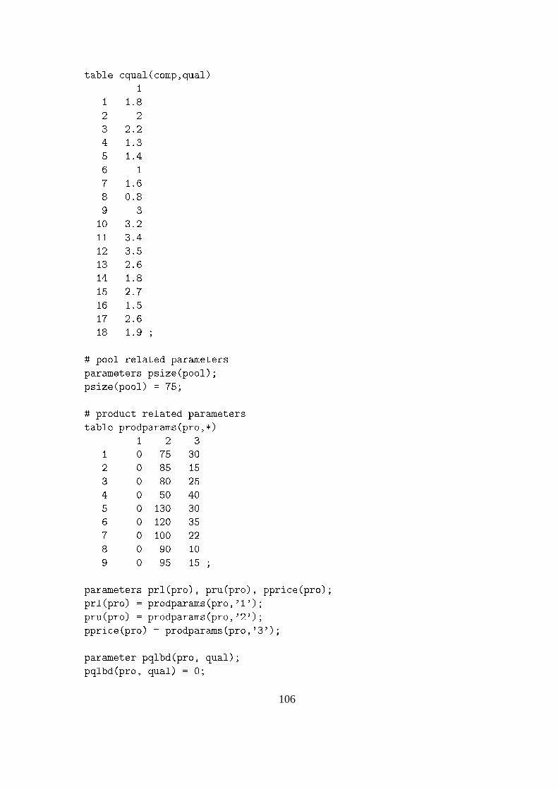
table qual( omp,qual)
1
1 1.8
2 2
3 2.2
4 1.3
5 1.4
6 1
7 1.6
8 0.8
9 3
10 3.2
11 3.4
12 3.5
13 2.6
14 1.8
15 2.7
16 1.5
17 2.6
18 1.9 ;
# pool related parameters
parameters psize(pool);
psize(pool) = 75;
# produ t related parameters
table prodparams(pro,*)
1 2 3
1 0 75 30
2 0 85 15
3 0 80 25
4 0 50 40
5 0 130 30
6 0 120 35
7 0 100 22
8 0 90 10
9 0 95 15 ;
parameters prl(pro), pru(pro), ppri e(pro);
prl(pro) = prodparams(pro,'1');
pru(pro) = prodparams(pro,'2');
ppri e(pro) = prodparams(pro,'3');
parameter pqlbd(pro, qual);
pqlbd(pro, qual) = 0;
106
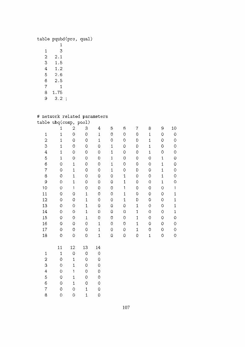
table pqubd(pro, qual)
1
1 3
2 2.1
3 1.5
4 1.2
5 2.6
6 2.5
7 1
8 1.75
9 3.2 ;
# network related parameters
table ubq( omp, pool)
1 2 3 4 5 6 7 8 9 10
1 1 0 0 1 0 0 0 1 0 0
2 1 0 0 1 0 0 0 1 0 0
3 1 0 0 0 1 0 0 1 0 0
4 1 0 0 0 1 0 0 1 0 0
5 1 0 0 0 1 0 0 0 1 0
6 0 1 0 0 1 0 0 0 1 0
7 0 1 0 0 1 0 0 0 1 0
8 0 1 0 0 0 1 0 0 1 0
9 0 1 0 0 0 1 0 0 1 0
10 0 1 0 0 0 1 0 0 0 1
11 0 0 1 0 0 1 0 0 0 1
12 0 0 1 0 0 1 0 0 0 1
13 0 0 1 0 0 0 1 0 0 1
14 0 0 1 0 0 0 1 0 0 1
15 0 0 1 0 0 0 1 0 0 0
16 0 0 0 1 0 0 1 0 0 0
17 0 0 0 1 0 0 1 0 0 0
18 0 0 0 1 0 0 0 1 0 0
11 12 13 14
1 1 0 0 0
2 0 1 0 0
3 0 1 0 0
4 0 1 0 0
5 0 1 0 0
6 0 1 0 0
7 0 0 1 0
8 0 0 1 0
107
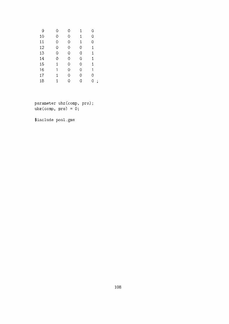
9 0 0 1 0
10 0 0 1 0
11 0 0 1 0
12 0 0 0 1
13 0 0 0 1
14 0 0 0 1
15 1 0 0 1
16 1 0 0 1
17 1 0 0 0
18 1 0 0 0 ;
parameter ubz( omp, pro);
ubz( omp, pro) = 0;
$in lude pool.gms
108
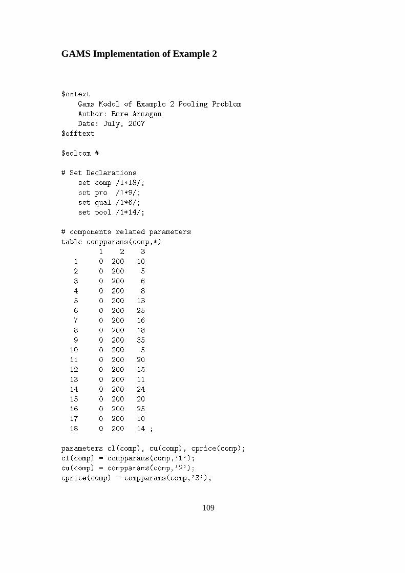
GAMS Implementation of Example 2
$ontext
Gams Model of Example 2 Pooling Problem
Author: Emre Armagan
Date: July, 2007
$offtext
$eol om #
# Set De larations
set omp /1*18/;
set pro /1*9/;
set qual /1*6/;
set pool /1*14/;
# omponents related parameters
table ompparams( omp,*)
1 2 3
1 0 200 10
2 0 200 5
3 0 200 6
4 0 200 8
5 0 200 13
6 0 200 25
7 0 200 16
8 0 200 18
9 0 200 35
10 0 200 5
11 0 200 20
12 0 200 15
13 0 200 11
14 0 200 24
15 0 200 20
16 0 200 25
17 0 200 10
18 0 200 14 ;
parameters l( omp), u( omp), pri e( omp);
l( omp) = ompparams( omp,'1');
u( omp) = ompparams( omp,'2');
pri e( omp) = ompparams( omp,'3');
109

table qual( omp,qual)
1 2 3 4 5 6
1 1.8 2.9 1.5 3 0.8 1.4
2 2.2 4.8 3.8 4.6 2.7 3.6
3 2 5 3 2.4 4 2
4 1.5 3.2 2.7 2.5 1.7 0.9
5 3.6 2.8 0.6 2 3.1 2
6 3.2 4.1 1.4 2.8 0.8 4.8
7 4 5 1.5 3.5 4.2 2.1
8 4.5 1.6 2.2 3.8 1.2 3
9 0.8 1.9 1.3 4 1.3 1.6
10 1.4 0.8 1.7 2.6 3.7 1.9
11 2.2 1.9 1.4 1 3.4 5
12 1.5 1 3.7 4.3 3.7 0.8
13 2.6 2.8 1.6 2.4 3.6 2
14 1.2 3.1 1.4 2.8 1 2.6
15 1.9 1.5 3.2 0.8 1.8 3.5
16 2.4 1.8 5 3.8 1.2 3
17 3.5 2.5 1.8 3.6 5 4.6
18 4.4 2.6 1.2 3 4.2 4 ;
# pool related parameters
parameters psize(pool);
psize(pool) = 75;
# produ t related parameters
table prodparams(pro,*)
1 2 3
1 0 75 30
2 0 85 15
3 0 80 25
4 0 50 40
5 0 130 30
6 0 120 35
7 0 100 22
8 0 90 10
9 0 95 15 ;
parameters prl(pro), pru(pro), ppri e(pro);
prl(pro) = prodparams(pro,'1');
pru(pro) = prodparams(pro,'2');
ppri e(pro) = prodparams(pro,'3');
parameter pqlbd(pro, qual);
pqlbd(pro, qual) = 0;
110
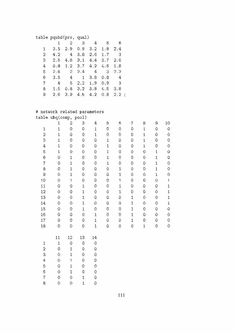
table pqubd(pro, qual)
1 2 3 4 5 6
1 3.5 2.9 0.9 3.2 1.8 2.4
2 4.2 4 3.8 2.6 1.7 3
3 2.5 4.8 3.1 4.4 3.7 2.6
4 0.8 1.2 3.7 4.2 4.6 1.8
5 2.6 2 2.4 4 3 2.2
6 3.5 4 1 3.8 0.8 4
7 4 5 2.2 1.9 0.9 3
8 1.5 0.8 3.2 3.8 4.5 3.8
9 2.6 3.9 4.5 4.2 0.8 2.2 ;
# network related parameters
table ubq( omp, pool)
1 2 3 4 5 6 7 8 9 10
1 1 0 0 1 0 0 0 1 0 0
2 1 0 0 1 0 0 0 1 0 0
3 1 0 0 0 1 0 0 1 0 0
4 1 0 0 0 1 0 0 1 0 0
5 1 0 0 0 1 0 0 0 1 0
6 0 1 0 0 1 0 0 0 1 0
7 0 1 0 0 1 0 0 0 1 0
8 0 1 0 0 0 1 0 0 1 0
9 0 1 0 0 0 1 0 0 1 0
10 0 1 0 0 0 1 0 0 0 1
11 0 0 1 0 0 1 0 0 0 1
12 0 0 1 0 0 1 0 0 0 1
13 0 0 1 0 0 0 1 0 0 1
14 0 0 1 0 0 0 1 0 0 1
15 0 0 1 0 0 0 1 0 0 0
16 0 0 0 1 0 0 1 0 0 0
17 0 0 0 1 0 0 1 0 0 0
18 0 0 0 1 0 0 0 1 0 0
11 12 13 14
1 1 0 0 0
2 0 1 0 0
3 0 1 0 0
4 0 1 0 0
5 0 1 0 0
6 0 1 0 0
7 0 0 1 0
8 0 0 1 0
111
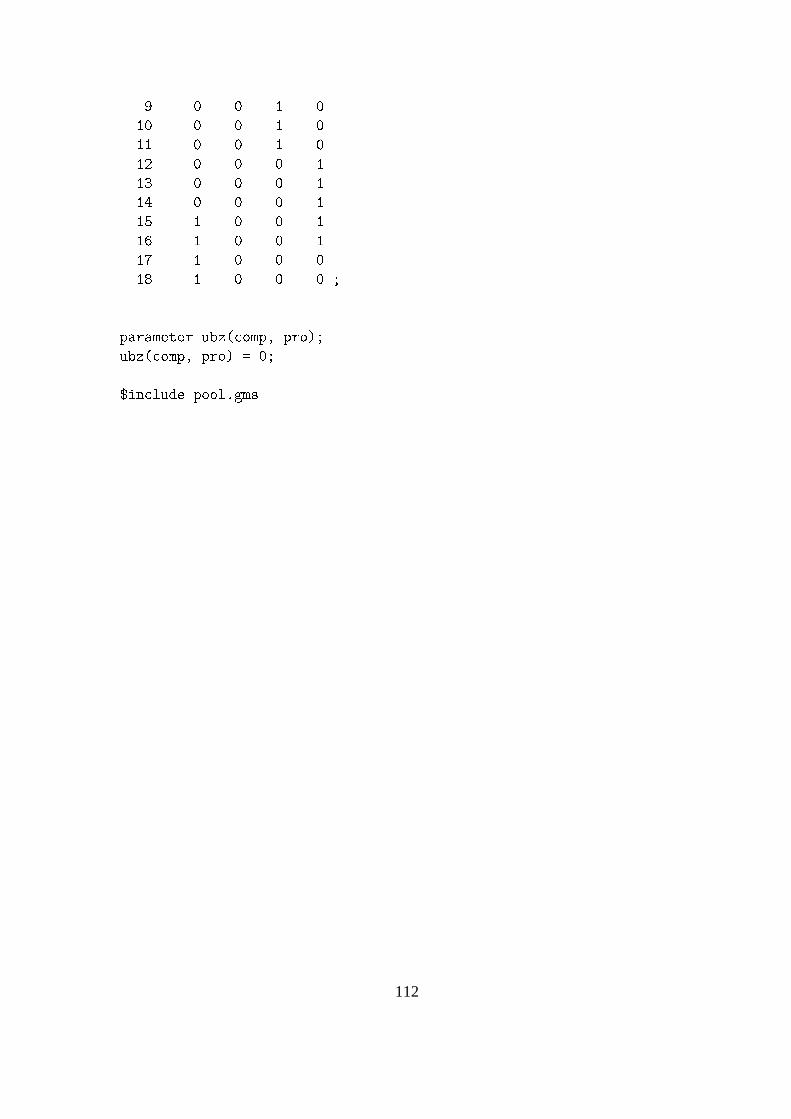
9 0 0 1 0
10 0 0 1 0
11 0 0 1 0
12 0 0 0 1
13 0 0 0 1
14 0 0 0 1
15 1 0 0 1
16 1 0 0 1
17 1 0 0 0
18 1 0 0 0 ;
parameter ubz( omp, pro);
ubz( omp, pro) = 0;
$in lude pool.gms
112

GAMS Implementation of Example 3
$ontext
Gams Model of Example 3 Pooling Problem
Author: Emre Armagan
Date: July, 2007
$offtext
$eol om #
# Set De larations
set omp /1*16/;
set pro /1*6/;
set qual /1*1/;
set pool /1*10/;
# omponents related parameters
table ompparams( omp,*)
1 2 3
1 0 100 30
2 0 100 40
3 0 100 45
4 0 100 38
5 0 100 18
6 0 100 30
7 0 100 32
8 0 100 45
9 0 100 55
10 0 100 50
11 0 100 20
12 0 100 19
13 0 100 20
14 0 100 28
15 0 100 30
16 0 100 45 ;
parameters l( omp), u( omp), pri e( omp);
l( omp) = ompparams( omp,'1');
u( omp) = ompparams( omp,'2');
pri e( omp) = ompparams( omp,'3');
table qual( omp,qual)
1
113
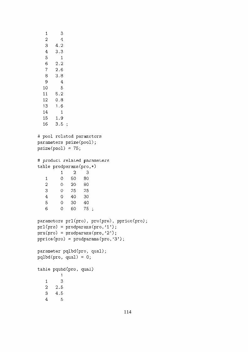
1 3
2 4
3 4.2
4 3.3
5 1
6 2.2
7 2.6
8 3.8
9 4
10 5
11 5.2
12 0.8
13 1.6
14 1
15 1.9
16 3.5 ;
# pool related parameters
parameters psize(pool);
psize(pool) = 75;
# produ t related parameters
table prodparams(pro,*)
1 2 3
1 0 50 80
2 0 20 90
3 0 25 25
4 0 40 30
5 0 30 40
6 0 60 75 ;
parameters prl(pro), pru(pro), ppri e(pro);
prl(pro) = prodparams(pro,'1');
pru(pro) = prodparams(pro,'2');
ppri e(pro) = prodparams(pro,'3');
parameter pqlbd(pro, qual);
pqlbd(pro, qual) = 0;
table pqubd(pro, qual)
1
1 3
2 2.5
3 4.5
4 5
114
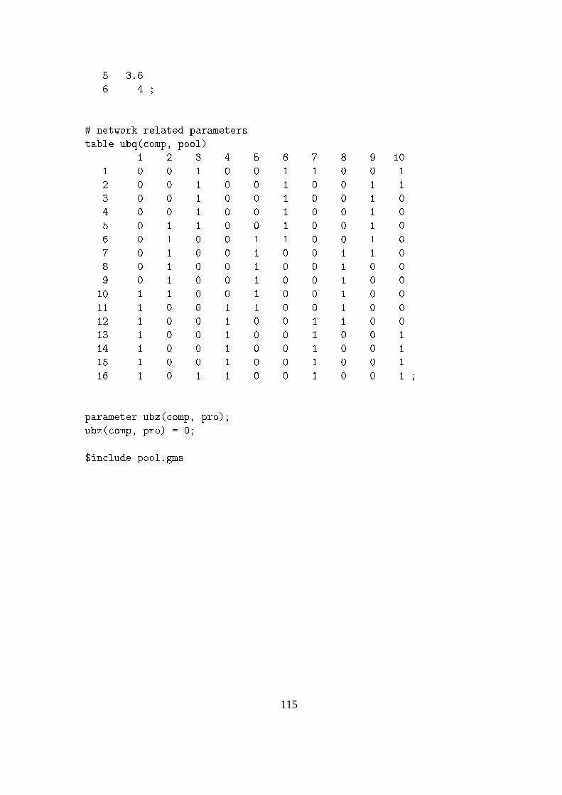
5 3.6
6 4 ;
# network related parameters
table ubq( omp, pool)
1 2 3 4 5 6 7 8 9 10
1 0 0 1 0 0 1 1 0 0 1
2 0 0 1 0 0 1 0 0 1 1
3 0 0 1 0 0 1 0 0 1 0
4 0 0 1 0 0 1 0 0 1 0
5 0 1 1 0 0 1 0 0 1 0
6 0 1 0 0 1 1 0 0 1 0
7 0 1 0 0 1 0 0 1 1 0
8 0 1 0 0 1 0 0 1 0 0
9 0 1 0 0 1 0 0 1 0 0
10 1 1 0 0 1 0 0 1 0 0
11 1 0 0 1 1 0 0 1 0 0
12 1 0 0 1 0 0 1 1 0 0
13 1 0 0 1 0 0 1 0 0 1
14 1 0 0 1 0 0 1 0 0 1
15 1 0 0 1 0 0 1 0 0 1
16 1 0 1 1 0 0 1 0 0 1 ;
parameter ubz( omp, pro);
ubz( omp, pro) = 0;
$in lude pool.gms
115
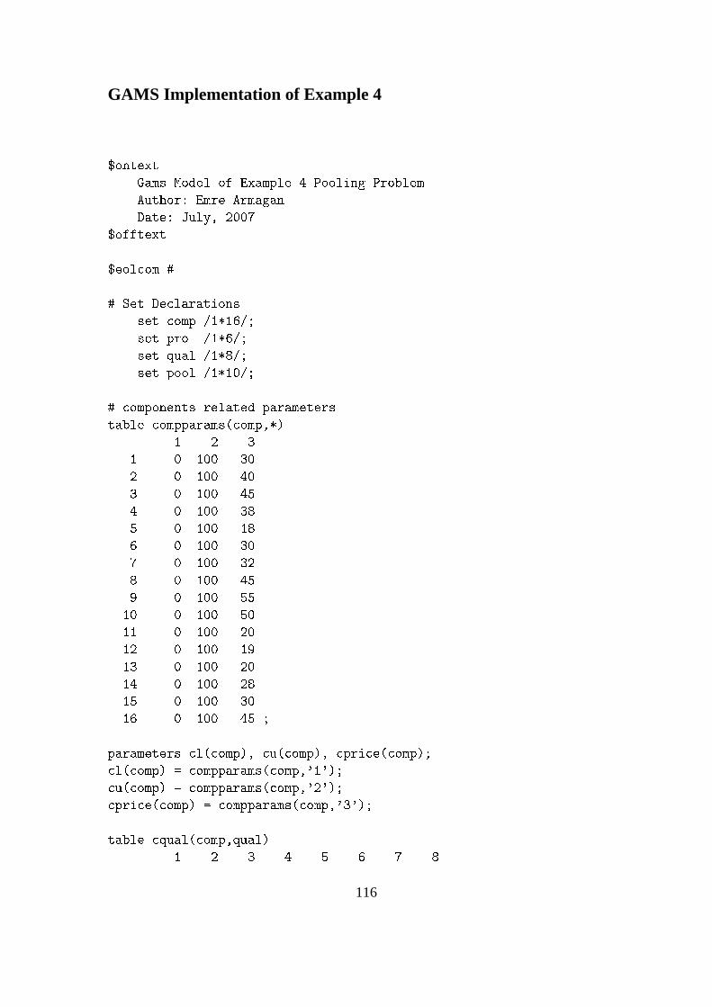
GAMS Implementation of Example 4
$ontext
Gams Model of Example 4 Pooling Problem
Author: Emre Armagan
Date: July, 2007
$offtext
$eol om #
# Set De larations
set omp /1*16/;
set pro /1*6/;
set qual /1*8/;
set pool /1*10/;
# omponents related parameters
table ompparams( omp,*)
1 2 3
1 0 100 30
2 0 100 40
3 0 100 45
4 0 100 38
5 0 100 18
6 0 100 30
7 0 100 32
8 0 100 45
9 0 100 55
10 0 100 50
11 0 100 20
12 0 100 19
13 0 100 20
14 0 100 28
15 0 100 30
16 0 100 45 ;
parameters l( omp), u( omp), pri e( omp);
l( omp) = ompparams( omp,'1');
u( omp) = ompparams( omp,'2');
pri e( omp) = ompparams( omp,'3');
table qual( omp,qual)
1 2 3 4 5 6 7 8
116
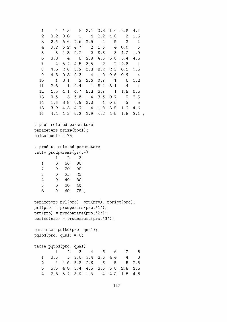
1 4 4.5 5 3.1 0.8 1.4 2.8 4.1
2 3.2 3.8 1 4 2.2 4.6 3 1.6
3 2.5 5.6 2.6 2.9 4 5 2 1
4 3.2 5.2 4.7 2 1.5 4 0.8 5
5 3 1.8 0.2 2 3.5 3 4.2 1.9
6 3.8 4 6 2.8 4.5 5.8 3.4 4.6
7 4 5.2 4.5 3.5 2 2 2.8 1
8 4.5 2.6 5.2 3.8 6.2 2.3 0.5 1.5
9 4.8 0.8 0.3 4 1.9 0.6 0.9 4
10 1 3.1 2 2.6 0.7 1 5 1.2
11 2.8 1 4.4 1 5.4 5.1 4 1
12 1.5 4.1 4.7 5.3 3.7 1 1.8 0.6
13 0.6 3 5.8 1.4 3.6 0.2 2 2.5
14 1.6 3.8 0.9 3.8 1 0.6 3 5
15 3.9 4.5 4.2 4 1.8 5.5 1.2 4.6
16 4.4 4.8 5.2 2.9 4.2 4.5 1.5 3.1 ;
# pool related parameters
parameters psize(pool);
psize(pool) = 75;
# produ t related parameters
table prodparams(pro,*)
1 2 3
1 0 50 80
2 0 20 90
3 0 25 25
4 0 40 30
5 0 30 40
6 0 60 75 ;
parameters prl(pro), pru(pro), ppri e(pro);
prl(pro) = prodparams(pro,'1');
pru(pro) = prodparams(pro,'2');
ppri e(pro) = prodparams(pro,'3');
parameter pqlbd(pro, qual);
pqlbd(pro, qual) = 0;
table pqubd(pro, qual)
1 2 3 4 5 6 7 8
1 3.6 5 2.8 3.4 2.6 4.4 4 3
2 4 4.6 5.8 2.6 6 5 5 2.5
3 5.5 4.8 3.4 4.5 3.5 3.6 2.8 3.6
4 2.8 5.2 3.9 1.5 4 4.8 1.8 4.6
117
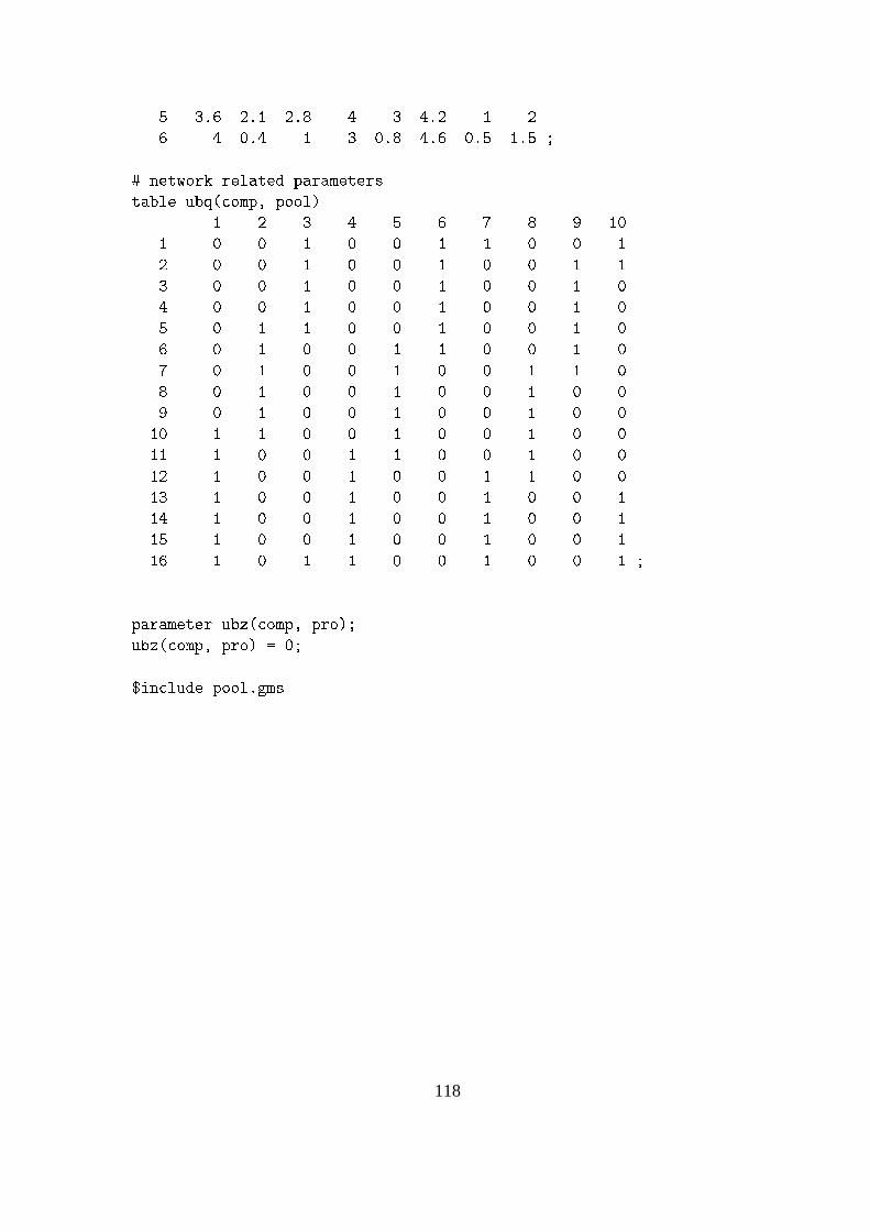
5 3.6 2.1 2.8 4 3 4.2 1 2
6 4 0.4 1 3 0.8 4.6 0.5 1.5 ;
# network related parameters
table ubq( omp, pool)
1 2 3 4 5 6 7 8 9 10
1 0 0 1 0 0 1 1 0 0 1
2 0 0 1 0 0 1 0 0 1 1
3 0 0 1 0 0 1 0 0 1 0
4 0 0 1 0 0 1 0 0 1 0
5 0 1 1 0 0 1 0 0 1 0
6 0 1 0 0 1 1 0 0 1 0
7 0 1 0 0 1 0 0 1 1 0
8 0 1 0 0 1 0 0 1 0 0
9 0 1 0 0 1 0 0 1 0 0
10 1 1 0 0 1 0 0 1 0 0
11 1 0 0 1 1 0 0 1 0 0
12 1 0 0 1 0 0 1 1 0 0
13 1 0 0 1 0 0 1 0 0 1
14 1 0 0 1 0 0 1 0 0 1
15 1 0 0 1 0 0 1 0 0 1
16 1 0 1 1 0 0 1 0 0 1 ;
parameter ubz( omp, pro);
ubz( omp, pro) = 0;
$in lude pool.gms
118
Appendix B
Gas Network Example
Gas network problems are a special kind of pooling problems where pools can be modeled
as mixers and splitters. Modeling pools as mixers and splitters gives the opportunity to
write mass balances for each quality separately.
For mixers, for a selected quality, mass balance can be written as the output volume
flow rate equals to the sums of input volume flow rates and it is alinear equation. In other
words, for the mixer shown in Figure B-1 (a), for a selected quality, mass balance can be
written asf3 = f1 + f2 where fi are flow variables and it is a linear equation. However, for
splitters, writing mass balances separately still introduces bilinear terms. In other words,
for the splitter shown in Figure B-1 (b), for a selected quality, mass balance can be written
asq1 f3 = q2 f1 +(1−q2) f2 where fi are flow variables;qi are quality variables and and
obviously, this equation is a bilinear equation. But, now since bilinear terms are only
coming from the splitters instead of all of the pools, the number of bilinear terms reduces
and therefore the complexity of the problem reduces greatly.
In order to test the performance of the proposed BD algorithm in a gas network problem,
an example problem shown in Figure B-2 is studied. As shown in the figure this problem
has 10 pools, 8 sources, 3 qualities and 4 end-products. Necessary parameters (quality
parameters, costs, prices and demand requirements) to construct this problem is given in
119
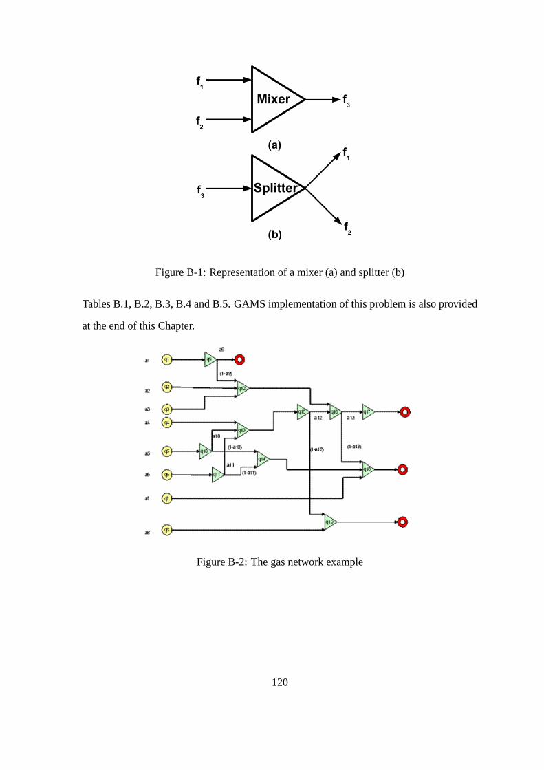
Figure B-1: Representation of a mixer (a) and splitter (b)
Tables B.1, B.2, B.3, B.4 and B.5. GAMS implementation of this problem is also provided
at the end of this Chapter.
Figure B-2: The gas network example
120

Source quality parametersSources Qualities
1 2 31 2.5 2.9 0.82 2.4 1.8 23 1 3 2.44 1.5 2 1.85 1.8 1.9 0.66 0.9 1.4 2.47 1.2 1.5 3.58 2.4 1.9 1
Table B.1: Quality parameters in source nodes for the gas network example
Source costsSources Costs
1 152 103 204 55 106 157 258 20
Table B.2: Cost parameters in source nodes for the gas network example
Demand quality requirementsProducts Qualities
1 2 31 2 2 32 3 1.5 23 1.5 3 1.54 2 2.5 0.75
Table B.3: Quality requirements in demand nodes for the gas network example
Demand flow requirementsProducts Max. flow
1 502 1003 754 80
Table B.4: Flow requirements in demand nodes for the gas network example
121

PricesProducts Prices
1 302 453 104 25
Table B.5: Prices in demand nodes for the gas network example
122
GAMS Implementation of Gas Network Example
$ontext
Gams Model of Gas network example
Author: Emre Armagan
Date: July, 2007
$offtext
$TITLE Natural Gas Network Optimization Model
SETS
NodeSet "Superset for Nodes"
Ar Set "Superset for Ar s"
Jun tions(NodeSet) "Set of jun tions where produ tion should be set to zero"
Wells(NodeSet) "Set of Wells"
Splitters(NodeSet) "Set of Splitter"
SplitOut(Splitters, Ar Set)
* Mixers(NodeSet) "Set of Mixer"
Demands "Set of demand"
dNodes(NodeSet) "Demand Nodes"
ddN(Demands, NodeSet) " orrelation set between the demands and node"
Components "Set of all omponents"
Spe ( omponents) " omponents on whi h spe ifi ation is for ed"
Ar Origin(Ar Set, NodeSet) "Ar origin to Node mapping"
Ar End(Ar Set, NodeSet) "Ar end to Node mapping";
PARAMETERS
fA(Ar Set) "fri tion fa tor onstant for ar s"
123
A(Wells) "Reservoir flow equation onstants"
B(Wells) "Reservoir flow equation onstants"
C(Wells) "Reservoir flow equation onstants"
F(Wells) "Reservoir flow equation onstants"
E(Wells) "sqrt(B)"
Pres(Wells) "Reservoir Pressure"
* IMPERIAL UNITS
fAi(Ar Set) "fri tion fa tor onstant for ar s"
Ai(Wells) "Reservoir flow equation onstants"
Bi(Wells) "Reservoir flow equation onstants"
Ci(Wells) "Reservoir flow equation onstants"
Fi(Wells) "Reservoir flow equation onstants"
D(Demands) "Demands"
Pdemand(Demands) "Requested Pressure at a demand"
MW(Components) "Mole ular Weight of omponents"
yspe (Demands, spe ) "Spe ifi ation ompositions on a omponent set
(Mole fra tion)";
SCALARS
Ti "Duration in days for a time interval"
rho "Density at standard temperature and pressure"
onvfa torP "Pressure onversion fa tor"
onvfa torV "Volumetri flow rate onversion fa tor"
onvfa tor1 "Intermediate fa tors"
onvfa tor2 "Intermediate fa tors"
onvfa tor3 "Intermediate fa tors"
onvfa tor4 "Intermediate fa tors"
PdropS alefa tor1 "S ale fa tor for Ar pressure drop"
PdropS alefa tor2 "S ale fa tor for Well pressure drop"
MoleS alefa tor "Flow s ale fa tor";
* P A R A M E T E R F I L E
$in lude gasplan-parameters
$ontext
Variable and Parameter Naming Conventions
fe = field exit (Gas olle tion Network exit, this is raw gas with liquids in)
124
e = ompressor exit
l = liquids
g = gases
sr = sour field
sw = sweet field
b = blending
fp= final field produ tion
i = omponent flows
ds = desulfurization fa ility in sour field
dh = dehydration by adsorption in the sweet field
= ompression
st = storage
in = in
out = out
f = omponent flows
$offtext
VARIABLES
* Obje tive value
z
* Quantities at Ea h Node
Mp f(NodeSet, Components) "Component flow at ea h node"
* Quantities at Ar s
PAin(Ar Set) "Pressure at the origin of an edge (equal to the node before it)"
PAout(Ar Set) "Pressure at end of the ar (x10 bar)"
MA(Ar Set) "Cumulative Flow in Ar (10^6 kg)"
MA f(Ar Set, Components) "Cumulative Component Flow in Ar (10^6 kg)"
QA(Ar Set) "Volumetri flow in Ar in u.m/day"
* Quantities at Wells
Pfbhp(Wells) "Flowing Bottom Hole Pressure for well"
Pfthp(Wells) "Flowing Tubing Head Pressure for well"
Qp(Wells) "Volumetri flow rates at the wells"
* Spliting Ratio
alpha(Splitters) "Split Fra tion"
* Demand variables
Fmolar(Demands, Components) "Component molar flow rate at demands"
FTmolar(Demands) "Total molar flow rate";
* x(Demands, Components) "Molar Composition at demands";
125
EQUATIONS
Ar PressureFlowRelation(Ar Set)
Ar MassVolumeRelation(Ar Set)
TotalAr Flow(Ar Set)
PositiveFlowConstraint(Ar Set)
NodeAr MassBalan e(NodeSet, Components)
Ar PressureRelationsN9A
Ar PressureRelationsN9B
Ar PressureRelationsN9C
Ar PressureRelationsN10A
Ar PressureRelationsN10B
Ar PressureRelationsN10C
Ar PressureRelationsN11A
Ar PressureRelationsN11B
Ar PressureRelationsN11C
Ar PressureRelationsN12A
Ar PressureRelationsN12B
Ar PressureRelationsN12C
Ar PressureRelationsN13A
Ar PressureRelationsN13B
Ar PressureRelationsN13C
Ar PressureRelationsN14A
Ar PressureRelationsN15A
Ar PressureRelationsN15B
Ar PressureRelationsN15C
Ar PressureRelationsN16A
Ar PressureRelationsN16B
Ar PressureRelationsN16C
Ar PressureRelationsN16D
Ar PressureRelationsN16E
126
Ar PressureRelationsN17A
Ar PressureRelationsN18A
Ar PressureRelationsN18B
Ar PressureRelationsN18C
Ar PressureRelationsN19A
Ar PressureRelationsN19B
Jun tionNodes(Jun tions, Components)
SplitterConstraintN9(Components)
SplitterConstraintN10(Components)
SplitterConstraintN11(Components)
SplitterConstraintN15(Components)
SplitterConstraintN16(Components)
BottomHolePressure(Wells)
TubingHeadPressure(Wells)
BHResRelation(Wells)
BHPTHPRelation1(Wells)
BHPTHPRelation2(Wells)
TubingHeadFlowConditionN1
TubingHeadFlowConditionN2
TubingHeadFlowConditionN3
TubingHeadFlowConditionN4
TubingHeadFlowConditionN5
TubingHeadFlowConditionN6
TubingHeadFlowConditionN7
TubingHeadFlowConditionN8
WellComponentFlows(Wells, Components)
DemandPressureConstraintN20
DemandPressureConstraintN21
DemandPressureConstraintN22
DemandPressureConstraintN23
127
DemandConstraint(Demands)
DemandMolarFlows(Demands, Components)
DemandMolarSpe ifi ation(Demands, Spe )
* DemandMolarComposition(Demands, Components)
DemandTotalMoleFlow(Demands)
Obje tive;
Ar PressureFlowRelation(Ar Set).. fA(Ar Set)*QA(Ar Set)*QA(Ar Set)
- PAin(Ar Set)*PAin(Ar Set) + PAout(Ar Set)*PAout(Ar Set) =E= 0;
Ar MassVolumeRelation(Ar Set).. MA(Ar Set) - QA(Ar Set)*rho*Ti =E= 0;
TotalAr Flow(Ar Set).. MA(Ar Set) - SUM(Components, MA f(Ar set, Components)) =E= 0;
PositiveFlowConstraint(Ar Set).. PAout(Ar Set) - PAin(Ar Set) =L= 0;
* RELATIONSHIP BETWEEN NODE and ARC VARIABLES
NodeAr MassBalan e(NodeSet, Components)..
SUM(Ar Set$Ar Origin(Ar Set, NodeSet), MA f(Ar Set, Components))
- SUM(Ar Set$Ar End(Ar Set, NodeSet), MA f(Ar Set, Components))
- Mp f(NodeSet, Components) =E= 0;
NodeAr MassBalan e(NodeSet)..
SUM(Ar Set, IN(NodeSet, Ar Set)*MA f(Ar Set))
=E= Mp f(NodeSet, Components) ;
Ar PressureRelationsN9A.. PAin('A9') - PAout('A1') =L= 0;
Ar PressureRelationsN9B.. PAin('A10') - PAout('A1') =L= 0;
Ar PressureRelationsN9C.. PAin('A9') - PAin('A10') =E= 0;
Ar PressureRelationsN10A.. PAin('A11') - PAout('A5') =L= 0;
Ar PressureRelationsN10B.. PAin('A12') - PAout('A5') =L= 0;
Ar PressureRelationsN10C.. PAin('A11') - PAin('A12') =E= 0;
Ar PressureRelationsN11A.. PAin('A13') - PAout('A6') =L= 0;
128

Ar PressureRelationsN11B.. PAin('A14') - PAout('A6') =L= 0;
Ar PressureRelationsN11C.. PAin('A13') - PAin('A14') =E= 0;
Ar PressureRelationsN12A.. PAin('A15') - PAout('A10') =L= 0;
Ar PressureRelationsN12B.. PAin('A15') - PAout('A2') =L= 0;
Ar PressureRelationsN12C.. PAin('A15') - PAout('A3') =L= 0;
Ar PressureRelationsN13A.. PAin('A16') - PAout('A4') =L= 0;
Ar PressureRelationsN13B.. PAin('A16') - PAout('A11') =L= 0;
Ar PressureRelationsN13C.. PAin('A16') - PAout('A13') =L= 0;
Ar PressureRelationsN14A.. PAin('A17') - PAout('A14') =L= 0;
Ar PressureRelationsN15A.. PAin('A18') - PAout('A16') =L= 0;
Ar PressureRelationsN15B.. PAin('A19') - PAout('A16') =L= 0;
Ar PressureRelationsN15C.. PAin('A18') - PAin('A19') =E= 0;
Ar PressureRelationsN16A.. PAin('A20') - PAout('A15') =L= 0;
Ar PressureRelationsN16B.. PAin('A21') - PAout('A15') =L= 0;
Ar PressureRelationsN16C.. PAin('A20') - PAout('A18') =L= 0;
Ar PressureRelationsN16D.. PAin('A21') - PAout('A18') =L= 0;
Ar PressureRelationsN16E.. PAin('A20') - PAin('A21') =E= 0;
Ar PressureRelationsN17A.. PAin('A22') - PAout('A20') =L= 0;
Ar PressureRelationsN18A.. PAin('A23') - PAout('A21') =L= 0;
Ar PressureRelationsN18B.. PAin('A23') - PAout('A17') =L= 0;
Ar PressureRelationsN18C.. PAin('A23') - PAout('A7') =L= 0;
Ar PressureRelationsN19A.. PAin('A24') - PAout('A19') =L= 0;
Ar PressureRelationsN19B.. PAin('A24') - PAout('A8') =L= 0;
* JUNCTION NODES
Jun tionNodes(Jun tions, Components).. Mp f(Jun tions, Components) =E= 0;
* SPLITTER CONSTRAINTS
SplitterConstraintN9(Components)..
MA f('A9', Components - alpha('N9')*MA f('A1',Components) =E= 0;
129
SplitterConstraintN10(Components)..
MA f('A11', Components) - alpha('N10')*MA f('A5',Components) =E= 0;
SplitterConstraintN11(Components)..
MA f('A13', Components) - alpha('N11')*MA f('A6',Components) =E= 0;
SplitterConstraintN15(Components)..
MA f('A18', Components) - alpha('N15')*MA f('A16',Components) =E= 0;
SplitterConstraintN16(Components)..
MA f('A20', Components) - alpha('N16')*(MA f('A15',Components)
+ MA f('A18',Components)) =E= 0;
* Well Constraints
BottomHolePressure(Wells)..
Pres(Wells)*Pres(Wells) - Pfbhp(Wells)*Pfbhp(Wells)
- A(Wells)*Qp(Wells) - F(Wells)*Qp(Wells)*Qp(Wells) =E= 0;
TubingHeadPressure(Wells)..
B(Wells)*Pfthp(Wells)*Pfthp(Wells) - Pfbhp(Wells)*Pfbhp(Wells)
- C(Wells)*Qp(Wells)*Qp(Wells) =E= 0;
BHResRelation(Wells).. Pfbhp(Wells)-Pres(Wells) =L= 0;
BHPTHPRelation1(Wells).. Pfthp(Wells)-Pfbhp(Wells) =L= 0;
BHPTHPRelation2(Wells).. Pfbhp(Wells) - E(Wells)*Pfthp(Wells) =L= 0;
TubingHeadFlowConditionN1.. PAin('A1') - Pfthp('N1') =L= 0 ;
TubingHeadFlowConditionN2.. PAin('A2') - Pfthp('N2')=L= 0 ;
TubingHeadFlowConditionN3.. PAin('A3') - Pfthp('N3')=L= 0 ;
TubingHeadFlowConditionN4.. PAin('A4') - Pfthp('N4') =L= 0 ;
TubingHeadFlowConditionN5.. PAin('A5') - Pfthp('N5')=L= 0 ;
TubingHeadFlowConditionN6.. PAin('A6') - Pfthp('N6')=L= 0 ;
TubingHeadFlowConditionN7.. PAin('A7') - Pfthp('N7') =L= 0 ;
TubingHeadFlowConditionN8.. PAin('A8') - Pfthp('N8')=L= 0 ;
WellComponentFlows(Wells, Components)..
Mp f(Wells, Components) - y(Wells,Components)*rho*Ti*Qp(Wells) =E= 0;
130
DemandConstraint(Demands)..
Ti*rho*D(Demands) + SUM(Components, SUM(dNodes$ddN(Demands, dNodes),
Mp f(dNodes, Components))) =L= 0;
DemandPressureConstraintN20.. Pdemand('d1') - PAout('A9') =L= 0;
DemandPressureConstraintN21.. Pdemand('d2') - PAout('A22') =L= 0;
DemandPressureConstraintN22.. Pdemand('d3') - PAout('A23') =L= 0;
DemandPressureConstraintN23.. Pdemand('d4') - PAout('A24') =L= 0;
DemandMolarFlows(Demands, Components)..
Fmolar(Demands, Components) + (SUM(dNodes$ddN(Demands, dNodes),
Mp f(dNodes, Components))*MoleS alefa tor)/MW(Components) =E= 0;
DemandMolarComposition(Demands, Components)..
x(Demands, Components)*FTmolar(Demands) =E= Fmolar(Demands, Components);
DemandMolarSpe ifi ation(Demands, Spe )..
Fmolar(Demands, Spe ) - yspe (Demands, Spe )*FTmolar(Demands) =L= 0;
DemandTotalMoleFlow(Demands)..
FTmolar(Demands) - SUM(Components, Fmolar(Demands, Components)) =E= 0;
Obje tive.. SUM((Components, dNodes), Mp f(dNodes, Components)) - z =E= 0;
MODEL GasProdu tionPlanning /all/;
$in lude gasplan-bounds
*$in lude lo al-solution
OPTION NLP=BARON;
OPTION Limrow = 20;
OPTION Lim ol = 20;
OPTION sysout=on;
GasProdu tionPlanning.optfile = 0;
SOLVE GasProdu tionPlanning USING NLP MINIMIZING z;
*file levels /lo al-solution.gms/;
*$in lude write-levels
131

132
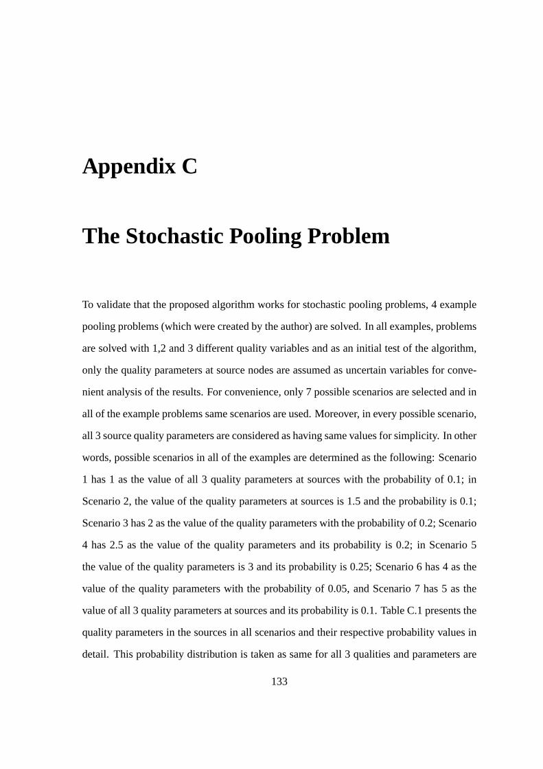
Appendix C
The Stochastic Pooling Problem
To validate that the proposed algorithm works for stochastic pooling problems, 4 example
pooling problems (which were created by the author) are solved. In all examples, problems
are solved with 1,2 and 3 different quality variables and as an initial test of the algorithm,
only the quality parameters at source nodes are assumed as uncertain variables for conve-
nient analysis of the results. For convenience, only 7 possible scenarios are selected and in
all of the example problems same scenarios are used. Moreover, in every possible scenario,
all 3 source quality parameters are considered as having same values for simplicity. In other
words, possible scenarios in all of the examples are determined as the following: Scenario
1 has 1 as the value of all 3 quality parameters at sources withthe probability of 0.1; in
Scenario 2, the value of the quality parameters at sources is1.5 and the probability is 0.1;
Scenario 3 has 2 as the value of the quality parameters with the probability of 0.2; Scenario
4 has 2.5 as the value of the quality parameters and its probability is 0.2; in Scenario 5
the value of the quality parameters is 3 and its probability is 0.25; Scenario 6 has 4 as the
value of the quality parameters with the probability of 0.05, and Scenario 7 has 5 as the
value of all 3 quality parameters at sources and its probability is 0.1. Table C.1 presents the
quality parameters in the sources in all scenarios and theirrespective probability values in
detail. This probability distribution is taken as same for all 3 qualities and parameters are
133

Probabilities of ScenariosScenarios Probabilities Source Qualities
1 2 31 0.1 1 1 12 0.1 1.5 1.5 1.53 0.2 2 2 24 0.2 2.5 2.5 2.55 0.25 3 3 36 0.05 4 4 47 0.1 5 5 5
Table C.1: Source quality parameters in scenarios and the respective probability values
Investment costs of poolsPools Costs
1 200
Table C.2: First stage investment costs of pools for Stochastic Example 1
used for all of them. When less than 3 quality variables is used, the remaining ones are ne-
glected (i.e. when 1 quality variable is considered, the parameters for the second and third
are neglected; when 2 quality variables are considered, theparameters for the third one
are neglected.). More information for both of these exampleproblems including quality
specs, demand requirements, cost coefficients is given in following sections. In addition,
GAMS implementation of the BD algorithm for stochastic programs is given in the end of
this chapter.
C.1 Stochastic Example 1
Example 1 has 1 pool, 3 sources, 2 end-products. Necessary parameters to construct this
problem is given in Tables C.2, C.3, C.4, C.5, C.6, C.7 and C.8.
134

Investment costs of pipesSources Pools
11 1002 503 100
Table C.3: First stage investment costs of pipelines (sources to pools) for Stochastic Exam-ple 1
Investment costs of pipesPools End-products
1 21 150 100
Table C.4: First stage investment costs of pipelines (pools to demands) for Stochastic Ex-ample 1
Source costsSources Costs
1 152 103 20
Table C.5: Second stage cost parameters in source nodes for Stochastic Example 1
Demand quality requirementsProducts Qualities
1 2 31 3 1 22 4 2 4
Table C.6: Second stage quality requirements in demand nodesfor Stochastic Example 1
Demand flow requirementsProducts Max. flow
1 1002 100
Table C.7: Second stage flow requirements in demand nodes for Stochastic Example 1
PricesProducts Prices
1 402 50
Table C.8: Second stage prices in demand nodes for StochasticExample 1
135

Investment costs of poolsPools Costs
1 4002 400
Table C.9: First stage investment costs of pools for Stochastic Example 2
Investment costs of pipesSources Pools
1 21 100 252 50 1503 100 2004 150 505 100 100
Table C.10: First stage investment costs of pipelines (sources to pools) for Stochastic Ex-ample 2
C.2 Stochastic Example 2
Example 2 has 2 pools, 5 sources, 3 end-products. Necessary parameters to construct this
problem is given in Tables C.9, C.10, C.11, C.12, C.13, C.14 and C.15.
Investment costs of pipesPools End-products
1 2 31 100 100 2002 50 30 75
Table C.11: First stage investment costs of pipelines (poolsto demands) for StochasticExample 2
136
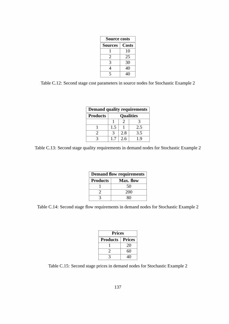
Source costsSources Costs
1 102 253 304 405 40
Table C.12: Second stage cost parameters in source nodes for Stochastic Example 2
Demand quality requirementsProducts Qualities
1 2 31 1.5 1 2.52 3 2.8 3.53 1.7 2.6 1.9
Table C.13: Second stage quality requirements in demand nodes for Stochastic Example 2
Demand flow requirementsProducts Max. flow
1 502 2003 80
Table C.14: Second stage flow requirements in demand nodes forStochastic Example 2
PricesProducts Prices
1 202 603 40
Table C.15: Second stage prices in demand nodes for Stochastic Example 2
137
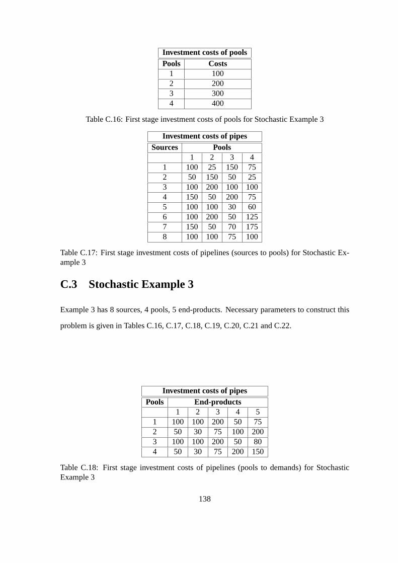
Investment costs of poolsPools Costs
1 1002 2003 3004 400
Table C.16: First stage investment costs of pools for Stochastic Example 3
Investment costs of pipesSources Pools
1 2 3 41 100 25 150 752 50 150 50 253 100 200 100 1004 150 50 200 755 100 100 30 606 100 200 50 1257 150 50 70 1758 100 100 75 100
Table C.17: First stage investment costs of pipelines (sources to pools) for Stochastic Ex-ample 3
C.3 Stochastic Example 3
Example 3 has 8 sources, 4 pools, 5 end-products. Necessary parameters to construct this
problem is given in Tables C.16, C.17, C.18, C.19, C.20, C.21 and C.22.
Investment costs of pipesPools End-products
1 2 3 4 51 100 100 200 50 752 50 30 75 100 2003 100 100 200 50 804 50 30 75 200 150
Table C.18: First stage investment costs of pipelines (poolsto demands) for StochasticExample 3
138
Source costsSources Costs
1 302 103 104 355 506 257 308 20
Table C.19: Second stage cost parameters in source nodes for Stochastic Example 3
Demand quality requirementsProducts Qualities
1 2 31 2 1.2 2.52 3 2 23 1.5 2.4 1.94 3 3 3.55 1.8 4 3.8
Table C.20: Second stage quality requirements in demand nodes for Stochastic Example 3
Demand flow requirementsProducts Max. flow
1 2002 2003 1004 2005 100
Table C.21: Second stage flow requirements in demand nodes forStochastic Example 3
PricesProducts Prices
1 302 103 504 755 40
Table C.22: Second stage prices in demand nodes for Stochastic Example 3
139
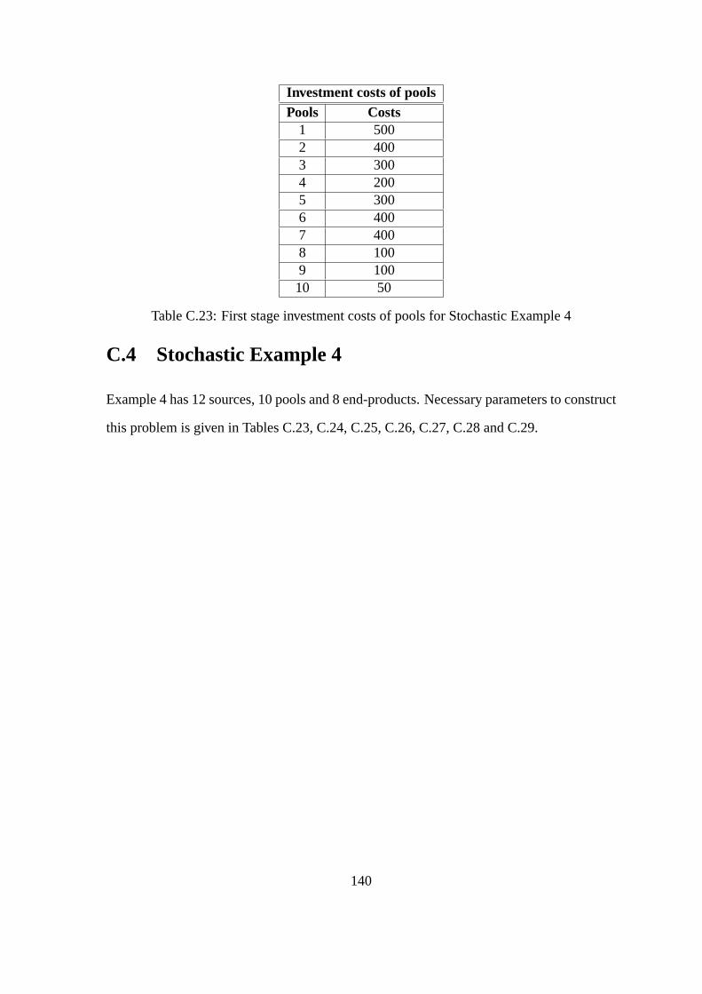
Investment costs of poolsPools Costs
1 5002 4003 3004 2005 3006 4007 4008 1009 10010 50
Table C.23: First stage investment costs of pools for Stochastic Example 4
C.4 Stochastic Example 4
Example 4 has 12 sources, 10 pools and 8 end-products. Necessary parameters to construct
this problem is given in Tables C.23, C.24, C.25, C.26, C.27, C.28 and C.29.
140
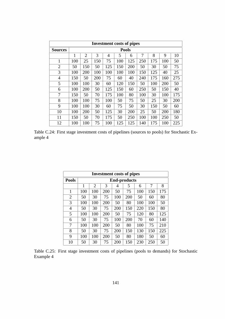
Investment costs of pipesSources Pools
1 2 3 4 5 6 7 8 9 101 100 25 150 75 100 125 250 175 100 502 50 150 50 125 150 200 50 30 50 753 100 200 100 100 100 100 150 125 40 254 150 50 200 75 60 40 240 175 160 2755 100 100 30 60 120 150 50 100 200 506 100 200 50 125 150 60 250 50 150 407 150 50 70 175 100 80 100 30 100 1758 100 100 75 100 50 75 50 25 30 2009 100 100 30 60 75 50 30 150 50 6010 100 200 50 125 30 200 25 50 200 18011 150 50 70 175 50 250 100 100 250 5012 100 100 75 100 125 125 140 175 100 225
Table C.24: First stage investment costs of pipelines (sources to pools) for Stochastic Ex-ample 4
Investment costs of pipesPools End-products
1 2 3 4 5 6 7 81 100 100 200 50 75 100 150 1752 50 30 75 100 200 50 60 803 100 100 200 50 80 100 100 504 50 30 75 200 150 220 150 805 100 100 200 50 75 120 80 1256 50 30 75 100 200 70 60 1407 100 100 200 50 80 100 75 2108 50 30 75 200 150 130 150 2259 100 100 200 50 80 180 50 6010 50 30 75 200 150 230 250 50
Table C.25: First stage investment costs of pipelines (poolsto demands) for StochasticExample 4
141
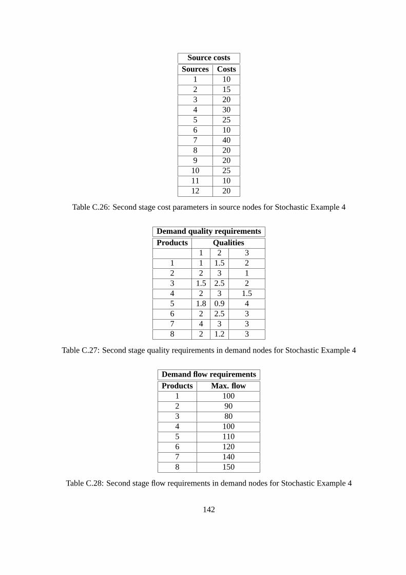
Source costsSources Costs
1 102 153 204 305 256 107 408 209 2010 2511 1012 20
Table C.26: Second stage cost parameters in source nodes for Stochastic Example 4
Demand quality requirementsProducts Qualities
1 2 31 1 1.5 22 2 3 13 1.5 2.5 24 2 3 1.55 1.8 0.9 46 2 2.5 37 4 3 38 2 1.2 3
Table C.27: Second stage quality requirements in demand nodes for Stochastic Example 4
Demand flow requirementsProducts Max. flow
1 1002 903 804 1005 1106 1207 1408 150
Table C.28: Second stage flow requirements in demand nodes forStochastic Example 4
142

PricesProducts Prices
1 302 403 504 605 206 307 158 20
Table C.29: Second stage prices in demand nodes for Stochastic Example 4
143
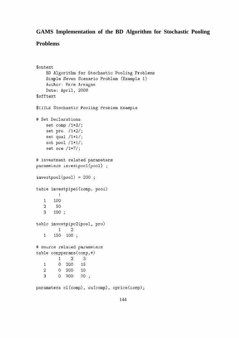
GAMS Implementation of the BD Algorithm for Stochastic Pooling
Problems
$ontext
BD Algorithm for Sto hasti Pooling Problems
Simple Seven S enario Problem (Example 1)
Author: Emre Armagan
Date: April, 2008
$offtext
$TITLE Sto hasti Pooling Problem Example
# Set De larations
set omp /1*3/;
set pro /1*2/;
set qual /1*1/;
set pool /1*1/;
set s e /1*7/;
# investment related parameters
parameters investpool(pool) ;
investpool(pool) = 200 ;
table investpipe1( omp, pool)
1
1 100
2 50
3 100 ;
table investpipe2(pool, pro)
1 2
1 150 100 ;
# sour e related parameters
table ompparams( omp,*)
1 2 3
1 0 200 15
2 0 200 10
3 0 200 20 ;
parameters l( omp), u( omp), pri e( omp);
144

l( omp) = ompparams( omp,'1');
u( omp) = ompparams( omp,'2');
pri e( omp) = ompparams( omp,'3');
# pool related parameters
parameters psize(pool);
psize(pool) = 200;
# produ t related parameters
table prodparams(pro,*)
1 2 3
1 0 100 40
2 0 100 50 ;
parameters prl(pro), pru(pro), ppri e(pro);
prl(pro) = prodparams(pro,'1');
pru(pro) = prodparams(pro,'2');
ppri e(pro) = prodparams(pro,'3');
parameter pqlbd(pro, qual);
pqlbd(pro, qual) = 0;
table pqubd(pro, qual)
1
1 3
2 4 ;
# s enario related parameters
table S e1( omp,qual)
1
1 1
2 1
3 1 ;
table S e2( omp,qual)
1
1 1.5
2 1.5
3 1.5 ;
table S e3( omp,qual)
1
1 2
2 2
3 2 ;
145
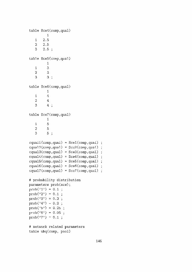
table S e4( omp,qual)
1
1 2.5
2 2.5
3 2.5 ;
table S e5( omp,qual)
1
1 3
2 3
3 3 ;
table S e6( omp,qual)
1
1 4
2 4
3 4 ;
table S e7( omp,qual)
1
1 5
2 5
3 5 ;
qual1( omp,qual) = S e1( omp,qual) ;
qual2( omp,qual) = S e2( omp,qual) ;
qual3( omp,qual) = S e3( omp,qual) ;
qual4( omp,qual) = S e4( omp,qual) ;
qual5( omp,qual) = S e5( omp,qual) ;
qual6( omp,qual) = S e6( omp,qual) ;
qual7( omp,qual) = S e7( omp,qual) ;
# probability distribution
parameters prob(s e);
prob('1') = 0.1 ;
prob('2') = 0.1 ;
prob('3') = 0.2 ;
prob('4') = 0.2 ;
prob('5') = 0.25 ;
prob('6') = 0.05 ;
prob('7') = 0.1 ;
# network related parameters
table ubq( omp, pool)
146
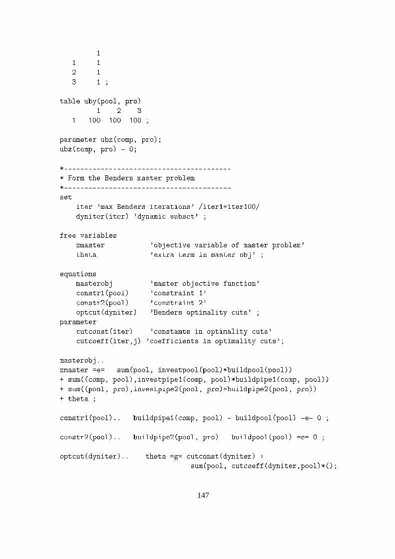
1
1 1
2 1
3 1 ;
table uby(pool, pro)
1 2 3
1 100 100 100 ;
parameter ubz( omp, pro);
ubz( omp, pro) = 0;
*-----------------------------------------
* Form the Benders master problem
*-----------------------------------------
set
iter 'max Benders iterations' /iter1*iter100/
dyniter(iter) 'dynami subset' ;
free variables
zmaster 'obje tive variable of master problem'
theta 'extra term in master obj' ;
equations
masterobj 'master obje tive fun tion'
onstr1(pool) ' onstraint 1'
onstr2(pool) ' onstraint 2'
opt ut(dyniter) 'Benders optimality uts' ;
parameter
ut onst(iter) ' onstants in optimality uts'
ut oeff(iter,j) ' oeffi ients in optimality uts';
masterobj..
zmaster =e= sum(pool, investpool(pool)*buildpool(pool))
+ sum(( omp, pool),investpipe1( omp, pool)*buildpipe1( omp, pool))
+ sum((pool, pro),investpipe2(pool, pro)*buildpipe2(pool, pro))
+ theta ;
onstr1(pool).. buildpipe1( omp, pool) - buildpool(pool) =e= 0 ;
onstr2(pool).. buildpipe2(pool, pro) - buildpool(pool) =e= 0 ;
opt ut(dyniter).. theta =g= ut onst(dyniter) +
sum(pool, ut oeff(dyniter,pool)*();
147
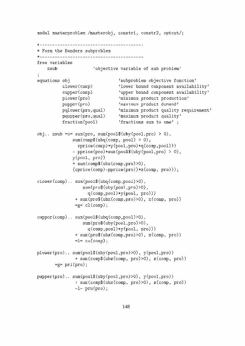
model masterproblem /masterobj, onstr1, onstr2, opt ut/;
*-----------------------------------------
* Form the Benders subproblem
*-----------------------------------------
free variables
zsub 'obje tive variable of sub problem'
;
equations obj 'subproblem obje tive fun tion'
lower( omp) 'lower bound omponent availability'
upper( omp) 'upper bound omponent availability'
plower(pro) 'minimum produ t produ tion'
pupper(pro) 'maximum produ t demand'
pqlower(pro,qual) 'minimum produ t quality requirement'
pqupper(pro,qual) 'maximum produ t quality'
fra tion(pool) 'fra tions sum to one' ;
obj.. zsub =e= sum(pro, sum(pool$(uby(pool,pro) > 0),
sum( omp$(ubq( omp, pool) > 0),
pri e( omp)*y(pool,pro)*q( omp,pool)))
- ppri e(pro)*sum(pool$(uby(pool,pro) > 0),
y(pool, pro))
+ sum( omp$(ubz( omp,pro)>0),
( pri e( omp)-ppri e(pro))*z( omp, pro)));
lower( omp).. sum(pool$(ubq( omp,pool)>0),
sum(pro$(uby(pool,pro)>0),
q( omp,pool)*y(pool, pro)))
+ sum(pro$(ubz( omp,pro)>0), z( omp, pro))
=g= l( omp);
upper( omp).. sum(pool$(ubq( omp,pool)>0),
sum(pro$(uby(pool,pro)>0),
q( omp,pool)*y(pool, pro)))
+ sum(pro$(ubz( omp,pro)>0), z( omp, pro))
=l= u( omp);
plower(pro).. sum(pool$(uby(pool,pro)>0), y(pool,pro))
+ sum( omp$(ubz( omp, pro)>0), z( omp, pro))
=g= prl(pro);
pupper(pro).. sum(pool$(uby(pool,pro)>0), y(pool,pro))
+ sum( omp$(ubz( omp, pro)>0), z( omp, pro))
=l= pru(pro);
148
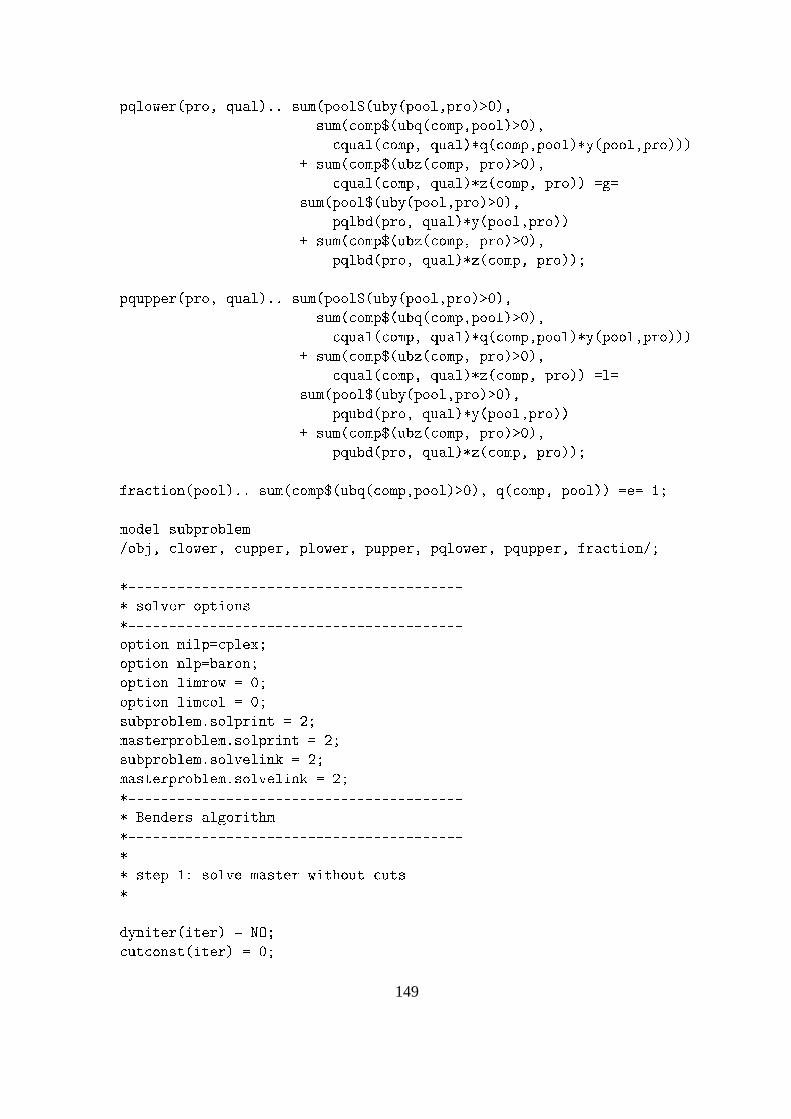
pqlower(pro, qual).. sum(pool$(uby(pool,pro)>0),
sum( omp$(ubq( omp,pool)>0),
qual( omp, qual)*q( omp,pool)*y(pool,pro)))
+ sum( omp$(ubz( omp, pro)>0),
qual( omp, qual)*z( omp, pro)) =g=
sum(pool$(uby(pool,pro)>0),
pqlbd(pro, qual)*y(pool,pro))
+ sum( omp$(ubz( omp, pro)>0),
pqlbd(pro, qual)*z( omp, pro));
pqupper(pro, qual).. sum(pool$(uby(pool,pro)>0),
sum( omp$(ubq( omp,pool)>0),
qual( omp, qual)*q( omp,pool)*y(pool,pro)))
+ sum( omp$(ubz( omp, pro)>0),
qual( omp, qual)*z( omp, pro)) =l=
sum(pool$(uby(pool,pro)>0),
pqubd(pro, qual)*y(pool,pro))
+ sum( omp$(ubz( omp, pro)>0),
pqubd(pro, qual)*z( omp, pro));
fra tion(pool).. sum( omp$(ubq( omp,pool)>0), q( omp, pool)) =e= 1;
model subproblem
/obj, lower, upper, plower, pupper, pqlower, pqupper, fra tion/;
*-----------------------------------------
* solver options
*-----------------------------------------
option milp= plex;
option nlp=baron;
option limrow = 0;
option lim ol = 0;
subproblem.solprint = 2;
masterproblem.solprint = 2;
subproblem.solvelink = 2;
masterproblem.solvelink = 2;
*-----------------------------------------
* Benders algorithm
*-----------------------------------------
*
* step 1: solve master without uts
*
dyniter(iter) = NO;
ut onst(iter) = 0;
149
ut oeff(iter,pool) = 0;
theta.fx = 0;
solve masterproblem minimizing zmaster using milp;
display zmaster.l;
*
* repair bounds
*
theta.lo = -INF;
theta.up = INF;
s alar lowerbound /-INF/;
s alar upperbound /INF/;
parameter objsub(s e);
s alar objmaster;
objmaster = zmaster.l;
s alar iteration;
s alar done /0/;
loop(iter$(not done),
iteration = ord(iter);
*
* solve subproblems
*
dyniter(iter) = yes;
loop(s e,
demnd(pool) = demand(pool,s e);
solve subproblem minimizing zsub using nlp;
objsub(s e) = zsub.l;
ut onst(iter) = ut onst(iter)-prob(s e)*(-plower.m(pro)-
lower.m( omp)- upper.m( omp)-pupper.m(pro)-pqlower.m(pro, qual)
-pqupper.m(pro, qual));
ut oeff(iter,pool) = ut oeff(iter,pool)-prob(s e)*(-plower.m(pro)-
lower.m( omp)- upper.m( omp)-pupper.m(pro)-pqlower.m(pro, qual)-
pqupper.m(pro, qual));
);
upperbound =
min(upperbound, objmaster + sum(s e, prob(s e)*objsub(s e)));
*
* onvergen e test
*
display lowerbound,upperbound;
if( (upperbound-lowerbound) < 0.001*(1+abs(lowerbound)),
display "Converged";
done = 1;
else
*
150
* solve masterproblem
*
solve masterproblem minimizing zmaster using milp;
lowerbound = zmaster.l;
objmaster = zmaster.l-theta.l;
);
);
abort$(not done) "Too many iterations";
display bd.log;
display zmaster, zsub;
151

152
Bibliography
[1] Adhya, N., Tawarmalani, M., Sahinidis, N. V. (1999). A lagrangian approach to the
pooling problem.Industrial & Engineering Chemistry, 38: 1956-1972.
[2] Androulakis, I. P., Visweswaran, V., Floudas, C. Distributed decomposition-based
approaches.State of the Art in Global Optimization: Computational Methods and
Applications. Kluwer Academic Publishers, Dordrecht, 1996.
[3] Audet, C., Brimberg, J., Hansen, P., Digabel, S., Mladenovic N. (2004). . Pooling
problem: alternate formulations and solutions method.Management Science, 50(6):
761-776.
[4] Barnes, R. J., Linke, P., Kokossis, A. (2002). Optimization of oil-field development
production capacity.European Symposium on Computer Aided Process Engineering,
12: 631-638.
[5] Benders, J. F. (1962). Partitioning procedures for solving mixed-variables program-
ming problems.Numerische Mathematik, 4: 238-252.
[6] Ben-Tal, A., Eiger, G., Gershovitz, V. (1994). Global minimization by reducing the
duality gap.Math. Programming, 63: 193-212.
[7] Birge, J. R., Louveaux, F.Introduction to stochastic programming. Springer, New
York, 1994.
153

[8] Brooke, A., Kendrick, D., Meeraus, A., Raman, R. (2004). GAMS: A user’s guide.
http://www.gams.com/docs/gams/GAMSUsersGuide.pdf.
[9] Dias, M. A. G. Selection of alternatives of investment ininformation for oil-field
development using evolutionary real options approach.Proceedings of 5th Annual
International Conference on Real Options. UCLA, Los Angeles, 2001.
[10] Energy Information Administration. (1990).Natural gas processing: the crucial link
between natural gas production and its transportation to market. Office of Oil and
Gas, Washington DC.
[11] Floudas, C. A., Aggarwal, A. (1990). A decomposition strategy for optimum search
in the pooling problem.ORSA Journal of Computation, 2 (3): 225-235.
[12] Foulds, L. R., Haugland, D., Jornsten, K. (1992). A bilinear approach to the pooling
problem.Optimization, 24: 165-180.
[13] The General Algebraic Modeling System (GAMS) (Version 22.5) [computer software].
GAMS Development Corporation, Washington DC, 2007.
[14] Geoffrion, A. M. (1972). Generalized benders decomposition. JOTA, 10 (4): 237-260.
[15] Goel, V., Grossmann, I. E., (2004). A stochastic programming approach to planning of
offshore gas field developments under uncertainty in reserves.Computers & Chemical
Engineering, 28: 1409-1429.
[16] Greenberg, H. J. (1995). Analyzing the pooling problem. ORSA Journal of Computa-
tion, 7 (2): 205-217.
[17] Guo, B., Ghalambor, A.Natural gas engineering handbook. Gulf Publishing, Hous-
ton, 2005.
154
[18] Haugen, K. K. (1996). A stochastic dynamic programmingmodel for scheduling of
offshore petroleum fields with resource uncertainty.European Journal of Operational
Research, 88: 88-95.
[19] Haverly, C. A. (1978). Studies of the behaviour of recursion for the pooling problem.
ACM SIGMAP Bull, 25: 29-32.
[20] Haverly, C. A. (1979). Behaviour of recursion model-morestudies.ACM SIGMAP
Bull, 26: 22-28.
[21] ILOG CPLEX (Version 10.2)[computer software]. ILOG Inc., Sunnyvale, CA, 2007.
[22] Iyer, R. R., Grossmann, I. E., Vasantharajan, S., Cullick,A. S. (1998). Optimal plan-
ning and scheduling of offshore oil field infrastructure investment and operations.
Industrial and Engineering Chemistry Research, 37: 1380-1392.
[23] Jonsbraten, T. W. (1998i). Oil-field optimization under price uncertainty.Journal of
the Operational Research Society, 49: 811-819.
[24] Jonsbraten, T. W., Wets, R. J. B., Woodruff, D. L. (1998). Aclass of stochastic pro-
grams with decision dependent random elements.Annals of Operations Research, 82:
83-88.
[25] Jonsbraten, T. W. (1998ii). Optimal selection and sequencing of oil wells under reser-
voir uncertainty.Ph.D. Thesis. Department of Business Administration, Stavanger
College, Norway.
[26] Jonsbraten, T. W. (1998iii). Nash equilibrium and bargaining in an oil reservoir man-
agement game.Journal of the Operational Research Society, 47: 356-362.
[27] Jonsbraten, T. W. (2001). Optimization models for petroleum field exploitation.An-
nals of Operations Research, 108: 121-130.
155
[28] Jornsten, K. O. (1992). Sequencing offshore oil and gasfields under uncertainty.Eu-
ropean Journal of Operational Research, 58: 191-199.
[29] Kall, P., Wallace, S.W.Stochastic programming. New York: Wiley, 1994.
[30] Lamar, B. W. (1993). An improved branch and bound algorithm for minimum concave
cost network flow problems.Journal of Global Optimization, 3: 261-287.
[31] Lasdon, L. S., Waren, A. D., Sarkar, S., Palacios-Gomez, F. (1979). Solving the pool-
ing problem using generalized reduced gradient and successive linear programming
algorithms.ACM SIGMAP Bull, 27: 9-15.
[32] Lin, X., Floudas, C. A. (2003). A novel continuous-time modeling and optimization
framework for well platform planning problems.Optimization and Engineering, 4:
65-93.
[33] Lund, M. W. (2000). Valuing flexibility in offshore petroleum projects.Annals of
Operations Research, 99: 325-332.
[34] Mangasarian, O. L., McLinden, L. (1985). Simple boundsfor solutions of monotone
complementarity problems, Mathematical Programming, 32:32-40.
[35] McCormick, G. P.Nonlinear programming. Theory, algorithms and applications. Wi-
ley Interscience: New York, 1983.
[36] Meister, B., Clark, J. M. C., Shah, N. (1996). Optimizationof oil-field exploitation
under uncertainty.Computers and Chemical Engineering, 20(B): 1242-1251.
[37] Ortiz-Gomez, A., Rico-Ramirez, V., Hernandez-Castro, S.(2002). Mixed-integer
multi-period model for the planning of oil-field production. Computers and Chem-
ical Engineering, 26(4-5): 703.
[38] Pflug, G. Ch. (1990). Online optimization of simulated markovian processes.Mathe-
matics of Operations Research, 15(3): 381-395.
156
[39] Ryoo, H. S., Sahinidis N. V. (1996). A branch-and-reduceapproach to global opti-
mization,Journal of Global Optimization, 8: 107-139.
[40] Sahinidis, N. V. (1996). BARON: a general purpose global optimization software
package.Journal of Global Optimization, 8: 201-205.
[41] Sahinidis, N. V., Grossmann, I. E. (1991). Convergence properties of generalized Ben-
ders decomposition.Computers and Chemical Engineering, 15 (7): 481-491.
[42] Sahinidis, N. V., Tawarmalani, M.Branch And Reduce Optimization Navigator
(BARON) (Version 7.8)[computer software]. Sahinidis Optimization Group, Pitts-
burgh, 2007.
[43] Savelsbergh M. W. P. (1994). Preprocessing and probingfor mixed integer program-
ming problems,ORSA Journal on Computing, 6: 445-454.
[44] Shectman, J. P., Sahinidis, N. V. (1998). A finite algorithm for global minimization of
separable concave programs,Journal of Global Optimization, 12: 1-36.
[45] Tawarmalani, M., Sahinidis, N. V.Convexification and global optimization in contin-
uous and mixed-integer nonlinear programming. Kluwer Academic Publishers, Dor-
drecht, 2002.
[46] Thakur, L. S. (1990). Domain contraction in nonlinear programming.Mathematics of
Operations Research, 16: 390-407.
[47] Van den Heever, S. A., Grossmann, I. E. (2000). An iterative aggregation/ disaggre-
gation approach for the solution of a mixed integer nonlinear oil-field infrastructure
planning model.Industrial and Engineering Chemistry Research, 39(6): 1955-1968.
[48] Van den Heever, S. A., Grossmann, I. E. (2001). A Lagrangean decomposition heuris-
tic for the design and planning of offshore hydrocarbon fieldinfrastructures with com-
157

plex economic objectives.Industrial and Engineering Chemistry Research, 40(13):
2843-2857.
[49] Visweswaran, V., Floudas, C. A. (1993). New properties and computational improve-
ment of the GOP algorithm for problems with quadratic objective functions and con-
straints.Journal of Global Optimization, 3: 439-462.
[50] Visweswaran, V., Floudas, C. A. New formulations and branching strategies for the
GOP algorithm.Global Optimization in Engineering Design. Kluwer Academic Pub-
lishers, Dordrecht, 1996.
[51] Zamora, J. M., Grossmann, I. E. (1999). A branch and contract algorithm for prob-
lems with cconcave univariate, bilinear, and linear fractional terms,Journal of Global
Optimization, 14: 217-249.
158