Embed Size (px)
Citation preview

Probability Review
Rob Hall
September 9, 2010
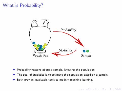
What is Probability?
I Probability reasons about a sample, knowing the population.
I The goal of statistics is to estimate the population based on a sample.
I Both provide invaluable tools to modern machine learning.
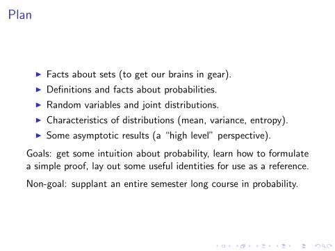
Plan
I Facts about sets (to get our brains in gear).
I Definitions and facts about probabilities.
I Random variables and joint distributions.
I Characteristics of distributions (mean, variance, entropy).
I Some asymptotic results (a “high level” perspective).
Goals: get some intuition about probability, learn how to formulatea simple proof, lay out some useful identities for use as a reference.
Non-goal: supplant an entire semester long course in probability.

Set Basics
A set is just a collection of elements denoted e.g.,S = s1, s2, s3,R = r : some condition holds on r.
I Intersection: the elements that are in both sets:A ∩ B = x : x ∈ A and x ∈ B
I Union: the elements that are in either set, or both:A ∪ B = x : x ∈ A or x ∈ B
I Complementation: all the elements that aren’t in the set:AC = x : x 6∈ A.
A BA ∩ B A ∪ B
AC
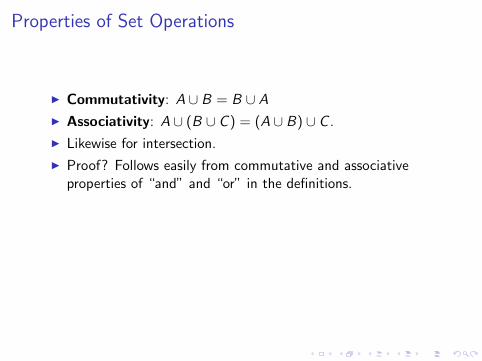
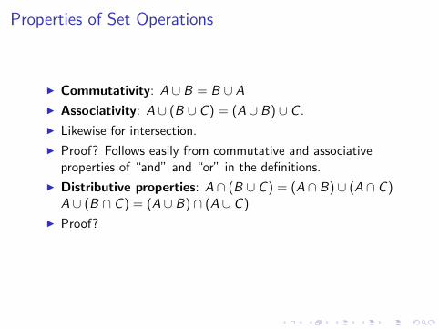
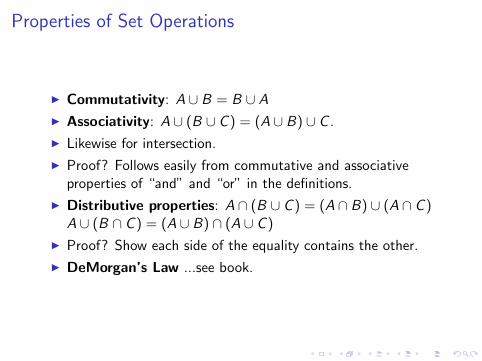
Properties of Set Operations
I Commutativity: A ∪ B = B ∪ A
I Associativity: A ∪ (B ∪ C ) = (A ∪ B) ∪ C .
I Likewise for intersection.
I Proof?
Follows easily from commutative and associativeproperties of “and” and “or” in the definitions.
I Distributive properties: A ∩ (B ∪ C ) = (A ∩ B) ∪ (A ∩ C )A ∪ (B ∩ C ) = (A ∪ B) ∩ (A ∪ C )
I Proof? Show each side of the equality contains the other.
I DeMorgan’s Law ...see book.
Properties of Set Operations
I Commutativity: A ∪ B = B ∪ A
I Associativity: A ∪ (B ∪ C ) = (A ∪ B) ∪ C .
I Likewise for intersection.
I Proof? Follows easily from commutative and associativeproperties of “and” and “or” in the definitions.
I Distributive properties: A ∩ (B ∪ C ) = (A ∩ B) ∪ (A ∩ C )A ∪ (B ∩ C ) = (A ∪ B) ∩ (A ∪ C )
I Proof?
Show each side of the equality contains the other.
I DeMorgan’s Law ...see book.
Properties of Set Operations
I Commutativity: A ∪ B = B ∪ A
I Associativity: A ∪ (B ∪ C ) = (A ∪ B) ∪ C .
I Likewise for intersection.
I Proof? Follows easily from commutative and associativeproperties of “and” and “or” in the definitions.
I Distributive properties: A ∩ (B ∪ C ) = (A ∩ B) ∪ (A ∩ C )A ∪ (B ∩ C ) = (A ∪ B) ∩ (A ∪ C )
I Proof? Show each side of the equality contains the other.
I DeMorgan’s Law ...see book.
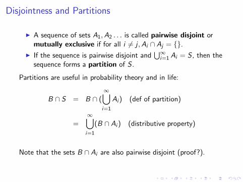
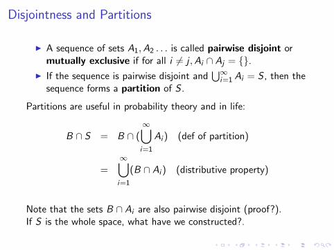
Disjointness and Partitions
I A sequence of sets A1,A2 . . . is called pairwise disjoint ormutually exclusive if for all i 6= j ,Ai ∩ Aj = .
I If the sequence is pairwise disjoint and⋃∞
i=1 Ai = S , then thesequence forms a partition of S .
Partitions are useful in probability theory and in life:
B ∩ S = B ∩ (∞⋃i=1
Ai ) (def of partition)
=∞⋃i=1
(B ∩ Ai ) (distributive property)
Note that the sets B ∩ Ai are also pairwise disjoint (proof?).
If S is the whole space, what have we constructed?.
Disjointness and Partitions
I A sequence of sets A1,A2 . . . is called pairwise disjoint ormutually exclusive if for all i 6= j ,Ai ∩ Aj = .
I If the sequence is pairwise disjoint and⋃∞
i=1 Ai = S , then thesequence forms a partition of S .
Partitions are useful in probability theory and in life:
B ∩ S = B ∩ (∞⋃i=1
Ai ) (def of partition)
=∞⋃i=1
(B ∩ Ai ) (distributive property)
Note that the sets B ∩ Ai are also pairwise disjoint (proof?).If S is the whole space, what have we constructed?.
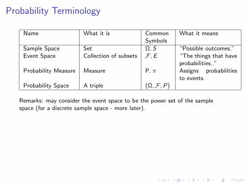
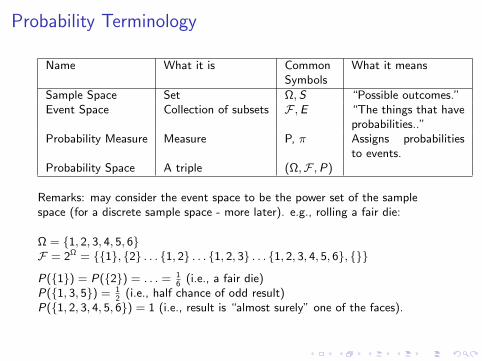
Probability Terminology
Name What it is CommonSymbols
What it means
Sample Space Set Ω, S “Possible outcomes.”Event Space Collection of subsets F ,E “The things that have
probabilities..”Probability Measure Measure P, π Assigns probabilities
to events.Probability Space A triple (Ω,F ,P)
Remarks: may consider the event space to be the power set of the samplespace (for a discrete sample space - more later).
e.g., rolling a fair die:
Ω = 1, 2, 3, 4, 5, 6F = 2Ω = 1, 2 . . . 1, 2 . . . 1, 2, 3 . . . 1, 2, 3, 4, 5, 6,
P(1) = P(2) = . . . = 16
(i.e., a fair die)P(1, 3, 5) = 1
2(i.e., half chance of odd result)
P(1, 2, 3, 4, 5, 6) = 1 (i.e., result is “almost surely” one of the faces).
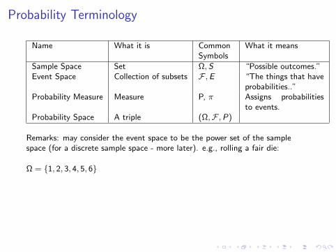
Probability Terminology
Name What it is CommonSymbols
What it means
Sample Space Set Ω, S “Possible outcomes.”Event Space Collection of subsets F ,E “The things that have
probabilities..”Probability Measure Measure P, π Assigns probabilities
to events.Probability Space A triple (Ω,F ,P)
Remarks: may consider the event space to be the power set of the samplespace (for a discrete sample space - more later). e.g., rolling a fair die:
Ω = 1, 2, 3, 4, 5, 6
F = 2Ω = 1, 2 . . . 1, 2 . . . 1, 2, 3 . . . 1, 2, 3, 4, 5, 6,
P(1) = P(2) = . . . = 16
(i.e., a fair die)P(1, 3, 5) = 1
2(i.e., half chance of odd result)
P(1, 2, 3, 4, 5, 6) = 1 (i.e., result is “almost surely” one of the faces).
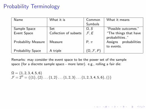
Probability Terminology
Name What it is CommonSymbols
What it means
Sample Space Set Ω, S “Possible outcomes.”Event Space Collection of subsets F ,E “The things that have
probabilities..”Probability Measure Measure P, π Assigns probabilities
to events.Probability Space A triple (Ω,F ,P)
Remarks: may consider the event space to be the power set of the samplespace (for a discrete sample space - more later). e.g., rolling a fair die:
Ω = 1, 2, 3, 4, 5, 6F = 2Ω = 1, 2 . . . 1, 2 . . . 1, 2, 3 . . . 1, 2, 3, 4, 5, 6,
P(1) = P(2) = . . . = 16
(i.e., a fair die)P(1, 3, 5) = 1
2(i.e., half chance of odd result)
P(1, 2, 3, 4, 5, 6) = 1 (i.e., result is “almost surely” one of the faces).

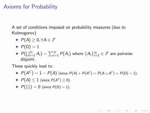
Axioms for Probability
A set of conditions imposed on probability measures (due toKolmogorov)
I P(A) ≥ 0,∀A ∈ FI P(Ω) = 1
I P(⋃∞
i=1 Ai ) =∑∞
i=1 P(Ai ) where Ai∞i=1 ∈ F are pairwisedisjoint.
These quickly lead to:
I P(AC ) = 1− P(A) (since P(A) + P(AC ) = P(A ∪ AC ) = P(Ω) = 1).
I P(A) ≤ 1 (since P(AC ) ≥ 0).
I P() = 0 (since P(Ω) = 1).

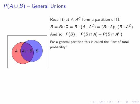
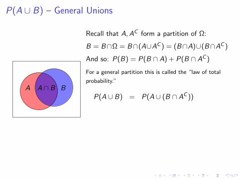
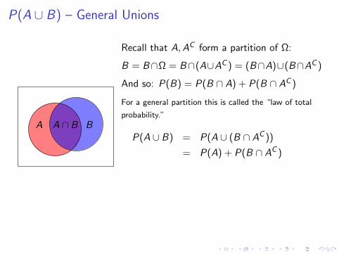
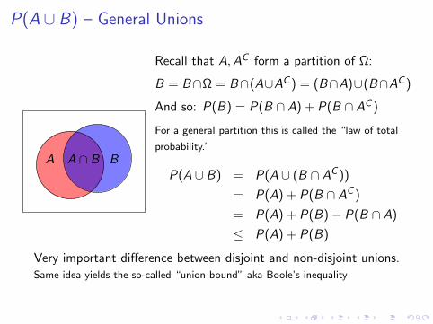
P(A ∪ B) – General Unions
A BA ∩ B
Recall that A,AC form a partition of Ω:
B = B∩Ω = B∩(A∪AC ) = (B∩A)∪(B∩AC )
And so: P(B) = P(B ∩ A) + P(B ∩ AC )
For a general partition this is called the “law of total
probability.”
P(A ∪ B) = P(A ∪ (B ∩ AC ))
= P(A) + P(B ∩ AC )
= P(A) + P(B)− P(B ∩ A)
≤ P(A) + P(B)
Very important difference between disjoint and non-disjoint unions.Same idea yields the so-called “union bound” aka Boole’s inequality
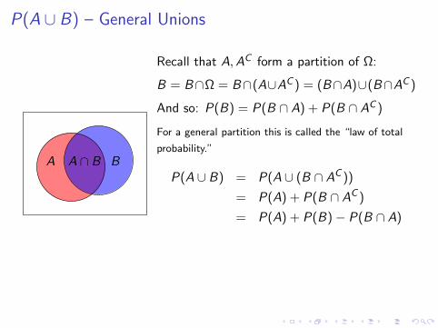
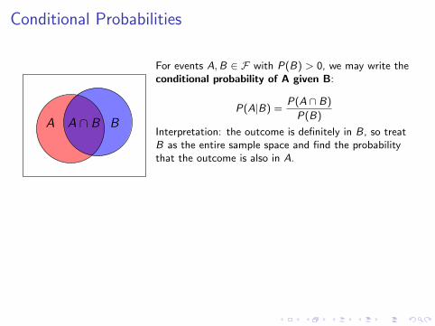
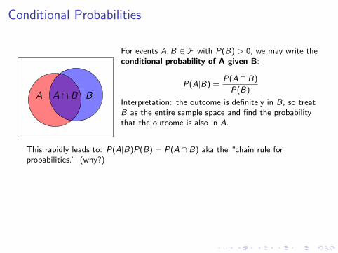
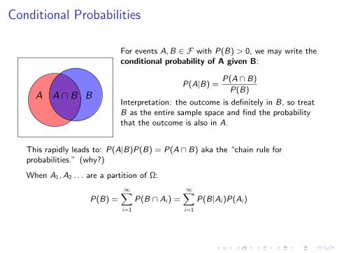
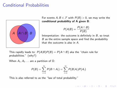
Conditional Probabilities
A BA ∩ B
For events A,B ∈ F with P(B) > 0, we may write theconditional probability of A given B:
P(A|B) =P(A ∩ B)
P(B)
Interpretation: the outcome is definitely in B, so treatB as the entire sample space and find the probabilitythat the outcome is also in A.
This rapidly leads to: P(A|B)P(B) = P(A ∩ B) aka the “chain rule forprobabilities.” (why?)
When A1,A2 . . . are a partition of Ω:
P(B) =∞∑i=1
P(B ∩ Ai ) =∞∑i=1
P(B|Ai )P(Ai )
This is also referred to as the “law of total probability.”
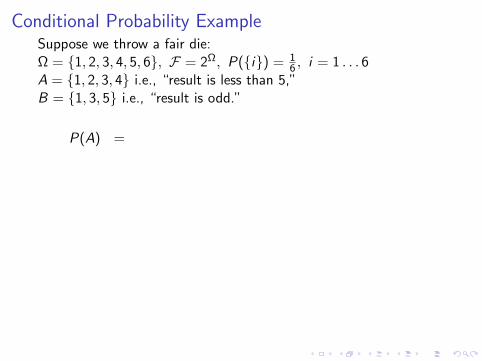
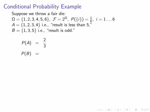
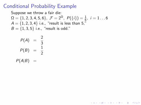
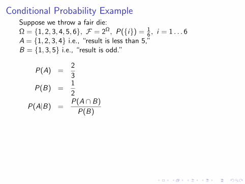
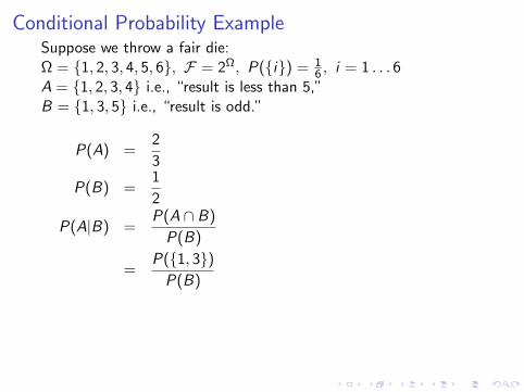
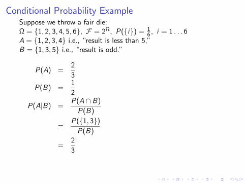
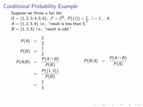
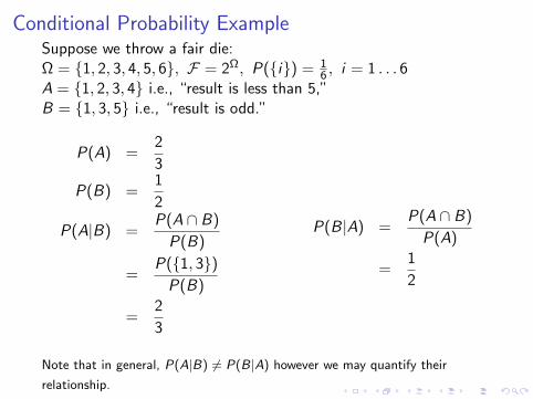
Conditional Probability ExampleSuppose we throw a fair die:Ω = 1, 2, 3, 4, 5, 6, F = 2Ω, P(i) = 1
6 , i = 1 . . . 6A = 1, 2, 3, 4 i.e., “result is less than 5,”B = 1, 3, 5 i.e., “result is odd.”
P(A) =
2
3
P(B) =1
2
P(A|B) =P(A ∩ B)
P(B)
=P(1, 3)
P(B)
=2
3
P(B|A) =P(A ∩ B)
P(A)
=1
2
Note that in general, P(A|B) 6= P(B|A) however we may quantify their
relationship.
Conditional Probability ExampleSuppose we throw a fair die:Ω = 1, 2, 3, 4, 5, 6, F = 2Ω, P(i) = 1
6 , i = 1 . . . 6A = 1, 2, 3, 4 i.e., “result is less than 5,”B = 1, 3, 5 i.e., “result is odd.”
P(A) =2
3
P(B) =
1
2
P(A|B) =P(A ∩ B)
P(B)
=P(1, 3)
P(B)
=2
3
P(B|A) =P(A ∩ B)
P(A)
=1
2
Note that in general, P(A|B) 6= P(B|A) however we may quantify their
relationship.
Conditional Probability ExampleSuppose we throw a fair die:Ω = 1, 2, 3, 4, 5, 6, F = 2Ω, P(i) = 1
6 , i = 1 . . . 6A = 1, 2, 3, 4 i.e., “result is less than 5,”B = 1, 3, 5 i.e., “result is odd.”
P(A) =2
3
P(B) =1
2
P(A|B) =
P(A ∩ B)
P(B)
=P(1, 3)
P(B)
=2
3
P(B|A) =P(A ∩ B)
P(A)
=1
2
Note that in general, P(A|B) 6= P(B|A) however we may quantify their
relationship.
Conditional Probability ExampleSuppose we throw a fair die:Ω = 1, 2, 3, 4, 5, 6, F = 2Ω, P(i) = 1
6 , i = 1 . . . 6A = 1, 2, 3, 4 i.e., “result is less than 5,”B = 1, 3, 5 i.e., “result is odd.”
P(A) =2
3
P(B) =1
2
P(A|B) =P(A ∩ B)
P(B)
=P(1, 3)
P(B)
=2
3
P(B|A) =P(A ∩ B)
P(A)
=1
2
Note that in general, P(A|B) 6= P(B|A) however we may quantify their
relationship.
Conditional Probability ExampleSuppose we throw a fair die:Ω = 1, 2, 3, 4, 5, 6, F = 2Ω, P(i) = 1
6 , i = 1 . . . 6A = 1, 2, 3, 4 i.e., “result is less than 5,”B = 1, 3, 5 i.e., “result is odd.”
P(A) =2
3
P(B) =1
2
P(A|B) =P(A ∩ B)
P(B)
=P(1, 3)
P(B)
=2
3
P(B|A) =P(A ∩ B)
P(A)
=1
2
Note that in general, P(A|B) 6= P(B|A) however we may quantify their
relationship.
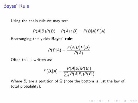
Bayes’ Rule
Using the chain rule we may see:
P(A|B)P(B) = P(A ∩ B) = P(B|A)P(A)
Rearranging this yields Bayes’ rule:
P(B|A) =P(A|B)P(B)
P(A)
Often this is written as:
P(Bi |A) =P(A|Bi )P(Bi )∑i P(A|Bi )P(Bi )
Where Bi are a partition of Ω (note the bottom is just the law oftotal probability).
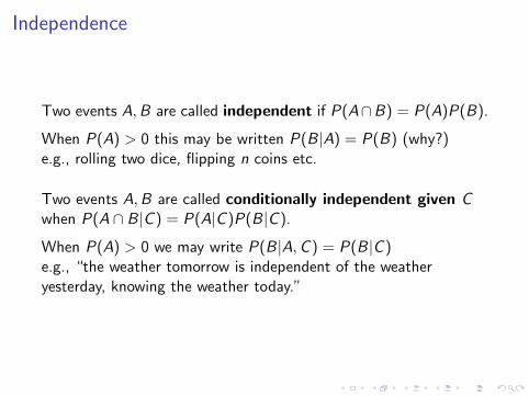
Independence
Two events A,B are called independent if P(A∩B) = P(A)P(B).
When P(A) > 0 this may be written P(B|A) = P(B) (why?)e.g., rolling two dice, flipping n coins etc.
Two events A,B are called conditionally independent given Cwhen P(A ∩ B|C ) = P(A|C )P(B|C ).
When P(A) > 0 we may write P(B|A,C ) = P(B|C )e.g., “the weather tomorrow is independent of the weatheryesterday, knowing the weather today.”
Independence
Two events A,B are called independent if P(A∩B) = P(A)P(B).
When P(A) > 0 this may be written P(B|A) = P(B) (why?)
e.g., rolling two dice, flipping n coins etc.
Two events A,B are called conditionally independent given Cwhen P(A ∩ B|C ) = P(A|C )P(B|C ).
When P(A) > 0 we may write P(B|A,C ) = P(B|C )e.g., “the weather tomorrow is independent of the weatheryesterday, knowing the weather today.”
Independence
Two events A,B are called independent if P(A∩B) = P(A)P(B).
When P(A) > 0 this may be written P(B|A) = P(B) (why?)e.g., rolling two dice, flipping n coins etc.
Two events A,B are called conditionally independent given Cwhen P(A ∩ B|C ) = P(A|C )P(B|C ).
When P(A) > 0 we may write P(B|A,C ) = P(B|C )e.g., “the weather tomorrow is independent of the weatheryesterday, knowing the weather today.”
Independence
Two events A,B are called independent if P(A∩B) = P(A)P(B).
When P(A) > 0 this may be written P(B|A) = P(B) (why?)e.g., rolling two dice, flipping n coins etc.
Two events A,B are called conditionally independent given Cwhen P(A ∩ B|C ) = P(A|C )P(B|C ).
When P(A) > 0 we may write P(B|A,C ) = P(B|C )
e.g., “the weather tomorrow is independent of the weatheryesterday, knowing the weather today.”
Independence
Two events A,B are called independent if P(A∩B) = P(A)P(B).
When P(A) > 0 this may be written P(B|A) = P(B) (why?)e.g., rolling two dice, flipping n coins etc.
Two events A,B are called conditionally independent given Cwhen P(A ∩ B|C ) = P(A|C )P(B|C ).
When P(A) > 0 we may write P(B|A,C ) = P(B|C )e.g., “the weather tomorrow is independent of the weatheryesterday, knowing the weather today.”

Random Variables – caution: hand waving
A random variable is a function X : Ω→ Rd
e.g.,
I Roll some dice, X = sum of the numbers.
I Indicators of events: X (ω) = 1A(ω). e.g., toss a coin, X = 1 if it cameup heads, 0 otherwise. Note relationship between the set theoreticconstructions, and binary RVs.
I Give a few monkeys a typewriter, X = fraction of overlap with completeworks of Shakespeare.
I Throw a dart at a board, X ∈ R2 are the coordinates which are hit.
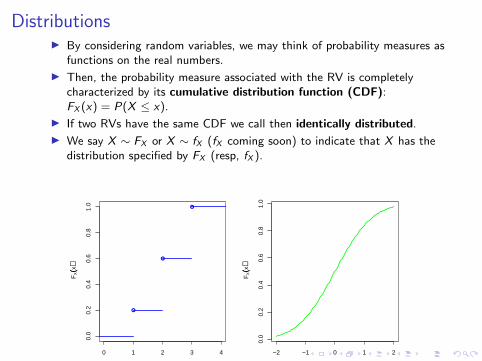
DistributionsI By considering random variables, we may think of probability measures as
functions on the real numbers.
I Then, the probability measure associated with the RV is completelycharacterized by its cumulative distribution function (CDF):FX (x) = P(X ≤ x).
I If two RVs have the same CDF we call then identically distributed.
I We say X ∼ FX or X ∼ fX (fX coming soon) to indicate that X has thedistribution specified by FX (resp, fX ).
0 1 2 3 4
0.0
0.2
0.4
0.6
0.8
1.0
x
FX((x
))
−2 −1 0 1 2
0.0
0.2
0.4
0.6
0.8
1.0
x
FX((x
))

Discrete Distributions
I If X takes on only a countable number of values, then we maycharacterize it by a probability mass function (PMF) whichdescribes the probability of each value: fX (x) = P(X = x).
I We have:∑
x fX (x) = 1 (why?) – since each ω maps to onex , and P(Ω) = 1.
I e.g., general discrete PMF: fX (xi ) = θi ,∑
i θi = 1, θi ≥ 0.
I e.g., bernoulli distribution: X ∈ 0, 1, fX (x) = θx(1− θ)1−x
I A general model of binary outcomes (coin flips etc.).
Discrete Distributions
I If X takes on only a countable number of values, then we maycharacterize it by a probability mass function (PMF) whichdescribes the probability of each value: fX (x) = P(X = x).
I We have:∑
x fX (x) = 1 (why?)
– since each ω maps to onex , and P(Ω) = 1.
I e.g., general discrete PMF: fX (xi ) = θi ,∑
i θi = 1, θi ≥ 0.
I e.g., bernoulli distribution: X ∈ 0, 1, fX (x) = θx(1− θ)1−x
I A general model of binary outcomes (coin flips etc.).

Discrete Distributions
I If X takes on only a countable number of values, then we maycharacterize it by a probability mass function (PMF) whichdescribes the probability of each value: fX (x) = P(X = x).
I We have:∑
x fX (x) = 1 (why?) – since each ω maps to onex , and P(Ω) = 1.
I e.g., general discrete PMF: fX (xi ) = θi ,∑
i θi = 1, θi ≥ 0.
I e.g., bernoulli distribution: X ∈ 0, 1, fX (x) = θx(1− θ)1−x
I A general model of binary outcomes (coin flips etc.).
Discrete Distributions
I If X takes on only a countable number of values, then we maycharacterize it by a probability mass function (PMF) whichdescribes the probability of each value: fX (x) = P(X = x).
I We have:∑
x fX (x) = 1 (why?) – since each ω maps to onex , and P(Ω) = 1.
I e.g., general discrete PMF: fX (xi ) = θi ,∑
i θi = 1, θi ≥ 0.
I e.g., bernoulli distribution: X ∈ 0, 1, fX (x) = θx(1− θ)1−x
I A general model of binary outcomes (coin flips etc.).
Discrete Distributions
I Rather than specifying each probability for each event, wemay consider a more restrictive parametric form, which will beeasier to specify and manipulate (but sometimes less general).
I e.g., multinomial distribution:X ∈ Nd ,
∑di=1 xi = n, fX (x) = n!
x1!x2!···xd !
∏di=1 θ
xii .
I Sometimes used in text processing (dimensions correspond towords, n is the length of a document).
I What have we lost in going from a general form to amultinomial?
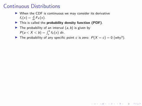
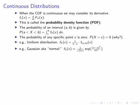
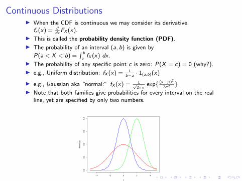
Continuous DistributionsI When the CDF is continuous we may consider its derivative
fx(x) = ddx
FX (x).
I This is called the probability density function (PDF).
I The probability of an interval (a, b) is given by
P(a < X < b) =∫ b
afX (x) dx .
I The probability of any specific point c is zero: P(X = c) = 0 (why?).
I e.g., Uniform distribution: fX (x) = 1b−a· 1(a,b)(x)
I e.g., Gaussian aka “normal:” fX (x) = 1√2πσ
exp (x−µ)2
2σ2 I Note that both families give probabilities for every interval on the real
line, yet are specified by only two numbers.
−4 −2 0 2 4
0.0
0.1
0.2
0.3
0.4
x
dnor
m (
x)
Continuous DistributionsI When the CDF is continuous we may consider its derivative
fx(x) = ddx
FX (x).
I This is called the probability density function (PDF).
I The probability of an interval (a, b) is given by
P(a < X < b) =∫ b
afX (x) dx .
I The probability of any specific point c is zero: P(X = c) = 0 (why?).
I e.g., Uniform distribution: fX (x) = 1b−a· 1(a,b)(x)
I e.g., Gaussian aka “normal:” fX (x) = 1√2πσ
exp (x−µ)2
2σ2
I Note that both families give probabilities for every interval on the realline, yet are specified by only two numbers.
−4 −2 0 2 4
0.0
0.1
0.2
0.3
0.4
x
dnor
m (
x)
Continuous DistributionsI When the CDF is continuous we may consider its derivative
fx(x) = ddx
FX (x).
I This is called the probability density function (PDF).
I The probability of an interval (a, b) is given by
P(a < X < b) =∫ b
afX (x) dx .
I The probability of any specific point c is zero: P(X = c) = 0 (why?).
I e.g., Uniform distribution: fX (x) = 1b−a· 1(a,b)(x)
I e.g., Gaussian aka “normal:” fX (x) = 1√2πσ
exp (x−µ)2
2σ2 I Note that both families give probabilities for every interval on the real
line, yet are specified by only two numbers.
−4 −2 0 2 4
0.0
0.1
0.2
0.3
0.4
x
dnor
m (
x)

Multiple Random Variables
We may consider multiple functions of the same sample space,e.g., X (ω) = 1A(ω),Y (ω) = 1B(ω):
A
BA ∩ B May represent the joint distribution as atable:
X=0 X=1
Y=0 0.25 0.15
Y=1 0.35 0.25
We write the joint PMF or PDF as fX ,Y (x , y)
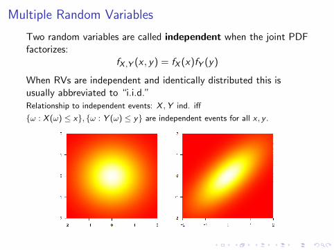
Multiple Random Variables
Two random variables are called independent when the joint PDFfactorizes:
fX ,Y (x , y) = fX (x)fY (y)
When RVs are independent and identically distributed this isusually abbreviated to “i.i.d.”Relationship to independent events: X ,Y ind. iff
ω : X (ω) ≤ x, ω : Y (ω) ≤ y are independent events for all x , y .
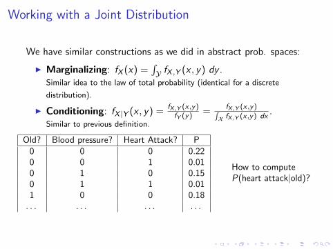
Working with a Joint Distribution
We have similar constructions as we did in abstract prob. spaces:
I Marginalizing: fX (x) =∫Y fX ,Y (x , y) dy .
Similar idea to the law of total probability (identical for a discrete
distribution).
I Conditioning: fX |Y (x , y) =fX ,Y (x ,y)
fY (y) =fX ,Y (x ,y)∫
X fX ,Y (x ,y) dx.
Similar to previous definition.
Old? Blood pressure? Heart Attack? P0 0 0 0.220 0 1 0.010 1 0 0.150 1 1 0.011 0 0 0.18
. . . . . . . . . . . .
How to computeP(heart attack|old)?
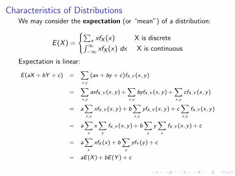
Characteristics of DistributionsWe may consider the expectation (or “mean”) of a distribution:
E (X ) =
∑x xfX (x) X is discrete∫∞−∞ xfX (x) dx X is continuous
Expectation is linear:
E(aX + bY + c) =∑x,y
(ax + by + c)fX ,Y (x , y)
=∑x,y
axfX ,Y (x , y) +∑x,y
byfX ,Y (x , y) +∑x,y
cfX ,Y (x , y)
= a∑x,y
xfX ,Y (x , y) + b∑x,y
yfX ,Y (x , y) + c∑x,y
fX ,Y (x , y)
= a∑
x
x∑
y
fX ,Y (x , y) + b∑
y
y∑
x
fX ,Y (x , y) + c
= a∑
x
xfX (x) + b∑
y
yfY (y) + c
= aE(X ) + bE(Y ) + c
Characteristics of Distributions
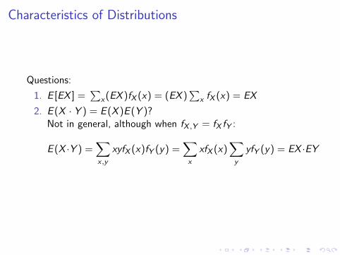
Questions:
1. E [EX ] =
∑x(EX )fX (x) = (EX )
∑x fX (x) = EX
2. E (X · Y ) = E (X )E (Y )?Not in general, although when fX ,Y = fX fY :
E (X ·Y ) =∑x ,y
xyfX (x)fY (y) =∑x
xfX (x)∑y
yfY (y) = EX ·EY
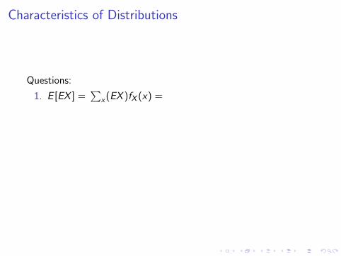
Characteristics of Distributions
Questions:
1. E [EX ] =∑
x(EX )fX (x) =
(EX )∑
x fX (x) = EX
2. E (X · Y ) = E (X )E (Y )?Not in general, although when fX ,Y = fX fY :
E (X ·Y ) =∑x ,y
xyfX (x)fY (y) =∑x
xfX (x)∑y
yfY (y) = EX ·EY

Characteristics of Distributions
Questions:
1. E [EX ] =∑
x(EX )fX (x) = (EX )∑
x fX (x) = EX
2. E (X · Y ) = E (X )E (Y )?Not in general, although when fX ,Y = fX fY :
E (X ·Y ) =∑x ,y
xyfX (x)fY (y) =∑x
xfX (x)∑y
yfY (y) = EX ·EY
Characteristics of Distributions
Questions:
1. E [EX ] =∑
x(EX )fX (x) = (EX )∑
x fX (x) = EX
2. E (X · Y ) = E (X )E (Y )?
Not in general, although when fX ,Y = fX fY :
E (X ·Y ) =∑x ,y
xyfX (x)fY (y) =∑x
xfX (x)∑y
yfY (y) = EX ·EY
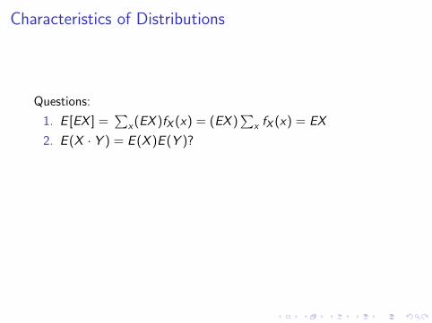
Characteristics of Distributions
Questions:
1. E [EX ] =∑
x(EX )fX (x) = (EX )∑
x fX (x) = EX
2. E (X · Y ) = E (X )E (Y )?Not in general, although when fX ,Y = fX fY :
E (X ·Y ) =∑x ,y
xyfX (x)fY (y) =∑x
xfX (x)∑y
yfY (y) = EX ·EY
Characteristics of Distributions
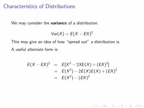
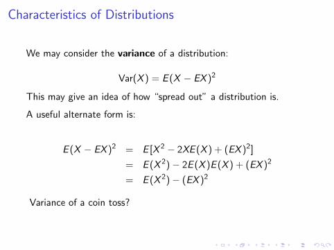
We may consider the variance of a distribution:
Var(X ) = E (X − EX )2
This may give an idea of how “spread out” a distribution is.
A useful alternate form is:
E (X − EX )2 = E [X 2 − 2XE (X ) + (EX )2]
= E (X 2)− 2E (X )E (X ) + (EX )2
= E (X 2)− (EX )2
Variance of a coin toss?
Characteristics of Distributions
We may consider the variance of a distribution:
Var(X ) = E (X − EX )2
This may give an idea of how “spread out” a distribution is.
A useful alternate form is:
E (X − EX )2 = E [X 2 − 2XE (X ) + (EX )2]
= E (X 2)− 2E (X )E (X ) + (EX )2
= E (X 2)− (EX )2
Variance of a coin toss?
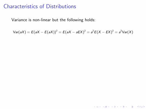
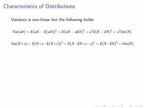
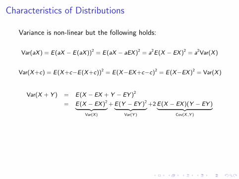
Characteristics of Distributions
Variance is non-linear but the following holds:
Var(aX ) = E(aX − E(aX ))2 = E(aX − aEX )2 = a2E(X − EX )2 = a2Var(X )
Var(X+c) = E(X+c−E(X+c))2 = E(X−EX+c−c)2 = E(X−EX )2 = Var(X )
Var(X + Y ) = E(X − EX + Y − EY )2
= E(X − EX )2︸ ︷︷ ︸Var(X )
+ E(Y − EY )2︸ ︷︷ ︸Var(Y )
+2 E(X − EX )(Y − EY )︸ ︷︷ ︸Cov(X ,Y )
So when X ,Y are independent we have:
Var(X + Y ) = Var(X ) + Var(Y )
(why?)
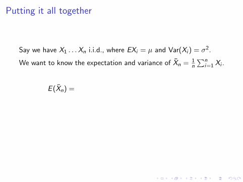
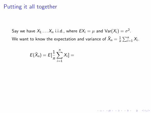
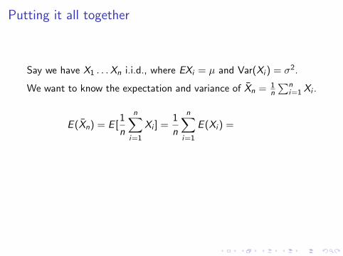
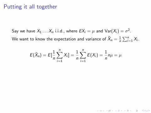
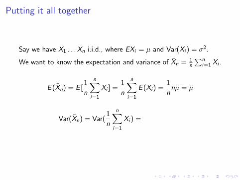
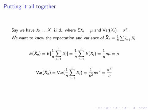
Putting it all together
Say we have X1 . . .Xn i.i.d., where EXi = µ and Var(Xi ) = σ2.
We want to know the expectation and variance of Xn = 1n
∑ni=1 Xi .
E (Xn) =
E [1
n
n∑i=1
Xi ] =1
n
n∑i=1
E (Xi ) =1
nnµ = µ
Var(Xn) = Var(1
n
n∑i=1
Xi ) =1
n2nσ2 =
σ2
n
Putting it all together
Say we have X1 . . .Xn i.i.d., where EXi = µ and Var(Xi ) = σ2.
We want to know the expectation and variance of Xn = 1n
∑ni=1 Xi .
E (Xn) = E [1
n
n∑i=1
Xi ] =
1
n
n∑i=1
E (Xi ) =1
nnµ = µ
Var(Xn) = Var(1
n
n∑i=1
Xi ) =1
n2nσ2 =
σ2
n
Putting it all together
Say we have X1 . . .Xn i.i.d., where EXi = µ and Var(Xi ) = σ2.
We want to know the expectation and variance of Xn = 1n
∑ni=1 Xi .
E (Xn) = E [1
n
n∑i=1
Xi ] =1
n
n∑i=1
E (Xi ) =
1
nnµ = µ
Var(Xn) = Var(1
n
n∑i=1
Xi ) =1
n2nσ2 =
σ2
n
Putting it all together
Say we have X1 . . .Xn i.i.d., where EXi = µ and Var(Xi ) = σ2.
We want to know the expectation and variance of Xn = 1n
∑ni=1 Xi .
E (Xn) = E [1
n
n∑i=1
Xi ] =1
n
n∑i=1
E (Xi ) =1
nnµ = µ
Var(Xn) = Var(1
n
n∑i=1
Xi ) =1
n2nσ2 =
σ2
n
Putting it all together
Say we have X1 . . .Xn i.i.d., where EXi = µ and Var(Xi ) = σ2.
We want to know the expectation and variance of Xn = 1n
∑ni=1 Xi .
E (Xn) = E [1
n
n∑i=1
Xi ] =1
n
n∑i=1
E (Xi ) =1
nnµ = µ
Var(Xn) = Var(1
n
n∑i=1
Xi ) =
1
n2nσ2 =
σ2
n
Putting it all together
Say we have X1 . . .Xn i.i.d., where EXi = µ and Var(Xi ) = σ2.
We want to know the expectation and variance of Xn = 1n
∑ni=1 Xi .
E (Xn) = E [1
n
n∑i=1
Xi ] =1
n
n∑i=1
E (Xi ) =1
nnµ = µ
Var(Xn) = Var(1
n
n∑i=1
Xi ) =1
n2nσ2 =
σ2
n

Entropy of a Distribution
Entropy is a measure of uniformity in a distribution.
H(X ) = −∑x
fX (x) log2 fX (x)
Imagine you had to transmit a sample from fX , so you constructthe optimal encoding scheme:
Entropy gives the mean depth in the tree (= mean number of bits).
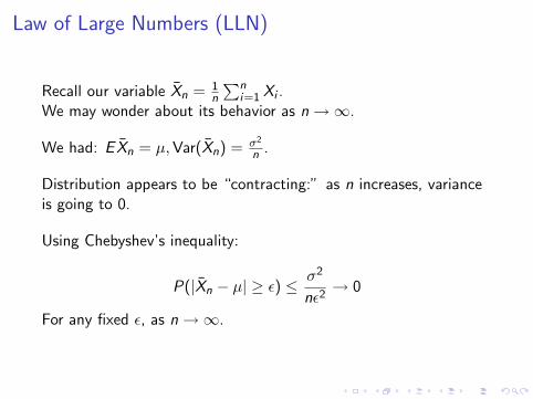
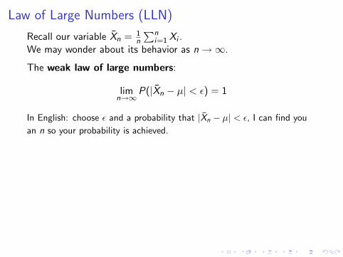
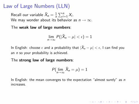
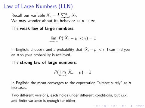
Law of Large Numbers (LLN)
Recall our variable Xn = 1n
∑ni=1 Xi .
We may wonder about its behavior as n→∞.
We had: EXn = µ,Var(Xn) = σ2
n .
Distribution appears to be “contracting:” as n increases, varianceis going to 0.
Using Chebyshev’s inequality:
P(|Xn − µ| ≥ ε) ≤σ2
nε2→ 0
For any fixed ε, as n→∞.
Law of Large Numbers (LLN)
Recall our variable Xn = 1n
∑ni=1 Xi .
We may wonder about its behavior as n→∞.
The weak law of large numbers:
limn→∞
P(|Xn − µ| < ε) = 1
In English: choose ε and a probability that |Xn − µ| < ε, I can find you
an n so your probability is achieved.
The strong law of large numbers:
P( limn→∞
Xn = µ) = 1
In English: the mean converges to the expectation “almost surely” as nincreases.
Two different versions, each holds under different conditions, but i.i.d.
and finite variance is enough for either.
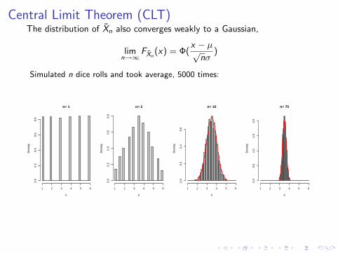
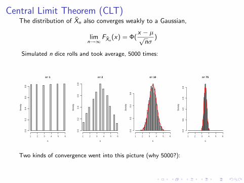
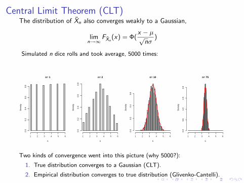
Central Limit Theorem (CLT)The distribution of Xn also converges weakly to a Gaussian,
limn→∞
FXn(x) = Φ(
x − µ√nσ
)
Simulated n dice rolls and took average, 5000 times:
n= 1
h
Den
sity
1 2 3 4 5 6
0.0
0.2
0.4
0.6
0.8
n= 2
h
Den
sity
1 2 3 4 5 6
0.0
0.2
0.4
0.6
0.8
n= 10
h
Den
sity
1 2 3 4 5 6
0.0
0.2
0.4
0.6
n= 75
h
Den
sity
1 2 3 4 5 6
0.0
0.5
1.0
1.5
2.0
Two kinds of convergence went into this picture (why 5000?):
1. True distribution converges to a Gaussian (CLT).
2. Empirical distribution converges to true distribution (Glivenko-Cantelli).
Asymptotics Opinion
Ideas like these are crucial to machine learning:
I We want to minimize error on a whole population (e.g.,classify text documents as well as possible)
I We minimize error on a training set of size n.
I What happens as n→∞?
I How does the complexity of the model, or the dimension ofthe problem affect convergence?