Embed Size (px)
Citation preview

Probabilities of Default and the Market Price of Risk in a Distressed Economy
Raphael Espinoza and Miguel Segoviano
WP/11/75
© 2011 International Monetary Fund WP/11/75 IMF Working Paper Strategy, Policy and Review Department
Probabilities of Default and the Market Price of Risk in a Distressed Economy
Prepared by Raphael Espinoza and Miguel Segoviano1
Authorized for distribution by Catherine Pattillo
April 2011
This Working Paper should not be reported as representing the views of the IMF. The views expressed in this Working Paper are those of the author(s) and do not necessarily represent those of the IMF or IMF policy. Working Papers describe research in progress by the author(s) and are published to elicit comments and to further debate.
Abstract
We propose an original method to estimate the market price of risk under stress, which is needed to correct for risk aversion the CDS-implied probabilities of distress. The method is based, for simplicity, on a one-factor asset pricing model. The market price of risk under stress (the expectation of the market price of risk, conditional on it exceeding a certain threshold) is computed from the price of risk (which is the variance of the market price of risk) and the discount factor (which is the inverse of the expected market price of risk). The threshold is endogenously determined so that the probability of the price of risk exceeding it is also the probability of distress of the asset. The price of risk can be estimated via different methods, for instance derived from the VIX or from the factors in a Fama-MacBeth regression. JEL Classification Numbers: G13; G21
Keywords: Price of risk; credit default swap; CDS; risk-neutral probability
Author’s E-Mail Address: [email protected]; [email protected]
1 Miguel Segoviano is Director General of Risk Analysis and Quantitative Methodologies at the Mexican Financial Authority (Comisión Nacional Bancaria y de Valores). The views expressed in this Working Paper are those of the authors and do not necessarily represent those of the IMF or of the Mexican Financial Authority. We are grateful to Thanawan Chaiwatana for outstanding research assistance. This paper benefitted greatly from discussions with Tobias Adrian, Carlos Caceres, Vincenzo Guizzo, Huyn Shyn, Dimitrios Tsomocos, and from participants at the IMF and at the LSE/CCBS Bank of England conference on Measuring Systemic Risk and Issues for Macroprudential Regulation. Any errors are solely the authors’ responsibility.

2
Contents Page
I. Introduction ............................................................................................................................3
II. Theoretical Background ........................................................................................................4 A. Risk-neutral Probabilities of Default and the Market Price of Risk .........................4 B. Conditional Expectation of the Market Price of Risk ...............................................6 C. Estimating the Price of Risk ......................................................................................7
III. Endogenous Threshold.........................................................................................................9
IV. Application to US Banks during the Crisis........................................................................11
V. Conclusion ..........................................................................................................................12
References ................................................................................................................................14
Figures Figure 1. Ratio of CDS-implied Probability of Distress to Moody’s KMV EDF .....................4 Figure 2. Uniqueness of the Threshold ....................................................................................10 Figure 3. Adjustment Factor and Market Price of Risk ...........................................................11 Figure 4. Estimated Probabilities of Default............................................................................13

3
I. INTRODUCTION
During the credit crisis of 2007-2009, the estimation of default probabilities of banks has been a focal point of interest. Default probabilities can be estimated using markets’ assessment, as captured by CDS spreads, or using models of the value of the firm derived from the Black-Scholes-Merton model (Black and Scholes, 1973; Merton, 1974). The latter method has been popularized by the Moody’s KMV Estimated Default Frequency (EDF) dataset, which provides default probabilities for many of the largest companies in the world, and most U.S. banks. CDS spreads are also widely used, although they are only proxies for default probabilities as they are influenced by the market price of risk (the cost of insurance) as well as the probabilities of distress of the firms. The two measures of probabilities of stress have diverged markedly during the post-Lehman times. We show in Figure 1 the ratio of the CDS-implied probability of default over the EDF probability of default for different U.S. banks. This ratio, which could be interpreted as the market price of insurance if the EDF and the CDS spread were representing perfectly the probability of default and the risk-neutral probability of default, has also varied dramatically across banks. It has been shown to vary across sectors (Berndt et al., 2005), and to correlate negatively with real activity (as one would expect from a pricing kernel–see section II) and positively with real interest rates (Amato, 2005, Amato and Luisi, 2006). The objective of this paper is to provide a method for computing the market price of risk under distress and therefore the probabilities of default implied by the CDS spreads. The objective is to provide an alternative measure to the EDFs, which are based on slowly-moving balance sheet information and have been lagging market information during the 2007-2009 crisis. The probabilities of distress in the recent abnormal times cannot be estimated using past data, so the method proposed by Jackwerth (2000) to compute risk aversion and actual probabilities is also ill-suited. In our paper, the calculations assume a one factor model (for instance a Consumption CAPM, although this is not needed for the results) and show how information on the mean and the variance of the factor can be used to derive the market price of risk under a situation of distress. This market price of risk is the conditional expectation of the price of risk, conditioning on it exceeding a threshold (section II). The factor we use is a transformation of the VIX (which has been shown to correlate strongly with the first principal component of asset returns). The approach is free of any assumption on the shape of the utility function (e.g., the coefficient of risk aversion) and of assumptions on stationarity of returns, but nonetheless it allows us to strip the effect of risk aversion on asset prices. However, the two fundamental assumptions are that pricing is based on a one-factor model, and that this factor is normally distributed.

4
Figure 1. Ratio of CDS-implied Probability of Distress to Moody’s KMV EDF
0
20
40
60
80
100
120
2-Ja
n-0
6
2-M
ar-0
6
2-M
ay-0
6
2-J
ul-0
6
2-S
ep-
06
2-N
ov-
06
2-Ja
n-0
7
2-M
ar-0
7
2-M
ay-0
7
2-J
ul-0
7
2-S
ep-
07
2-N
ov-
07
2-Ja
n-0
8
2-M
ar-0
8
2-M
ay-0
8
2-J
ul-0
8
2-S
ep-
08
2-N
ov-
08
2-Ja
n-0
9
2-M
ar-0
9
2-M
ay-0
9
AIG
AXP
BAC
GS
JPM
MS
WFC
Source: Moody’s KMV and Bloomberg We finally show that the market price of risk under distress has to be calculated jointly with the probability of distress to ensure the conditioning threshold is compatible with the probability of default (section III). We apply our method to the major U.S. banks during the crisis (section IV) and show that CDS-implied probabilities of default overestimated credit risk by roughly 50 percent. Section V concludes.
II. THEORETICAL BACKGROUND
A. Risk-neutral Probabilities of Default and the Market Price of Risk
In this section we review the basic asset pricing framework linking the price of risk to the CDS-implies probabilities of default. A one factor model can be derived from a consumption Euler equation:
11
)(
)(t
t
ttt x
cu
cuEP (1)
where tP is asset price at time t and 1tx is the one period-ahead payoff. The stochastic
discount factor is defined as
)(
)( 11
t
tt cu
cum
(2)
and the linear pricing formula for the one-factor model is therefore: ][ 11 tttt xmEP . (3)

5
Writing the gross return 1tR = t
t
P
x 1 , the pricing formula is equivalent to
][1 11 ttt RmE . (4)
Applying the previous equation to a risk-free asset:
][1 11f
ttt RmE or ][
1
11
tt
ft mE
R (5)
If the states of nature at time t+1 are indexed by s, and the probability of state s is ( )s
1 1( ) ( ) ( ) [ ]t t t ts
P s m s x s E m x (6)
The risk-neutral probability is such that2
1ˆ( ) ( ) ( )fts R m s s (7)
This probability measure does not correspond to any actual probability of nature-in particular it does not imply that the asset pricing model is based on risk-neutral investors. Nonetheless, the term “risk-neutral probability” is used in the literature because this is the probability measure that a risk-neutral investor would need to “believe in” to agree on the asset prices given by the markets. Indeed, the price of an asset can be written as
1 1
ˆ1 ( )ˆ( ) ( )t f f
st t
E xP s x s
R R
(8)
where )(ˆ xE is the expected value of xt+1 associated with the risk-neutral probability measure
. For a risk-neutral investor that believes that ˆ( )s are the actual probabilities of nature,
the price Pt given by the markets is coherent with the payoff xt+1. The risk-neutral probability ˆ( )s is what is obtained from CDS spreads. Indeed, ˆ( )s /Rt+1
is the price of an asset that pays x(s) = 1 dollar in the state of distress s (from equation 8). A
common approximation is ˆ(1 )
NS
K
where SN is the CDS spread of bank N and K the
recovery rate (assumed to be at 60 percent), and 1f
tR can be proxied by the OIS rate. The
missing element is therefore the market price of risk m(s).
2 is a probability measure since all (s) are positive (from the fundamental theorem of finance, m(s) is
positive in absence of arbitrage opportunities). Furthermore, 1ˆ ( ) ( ) ( ) [ ] 1f fd d t t
s s
s R m s s E R m
6
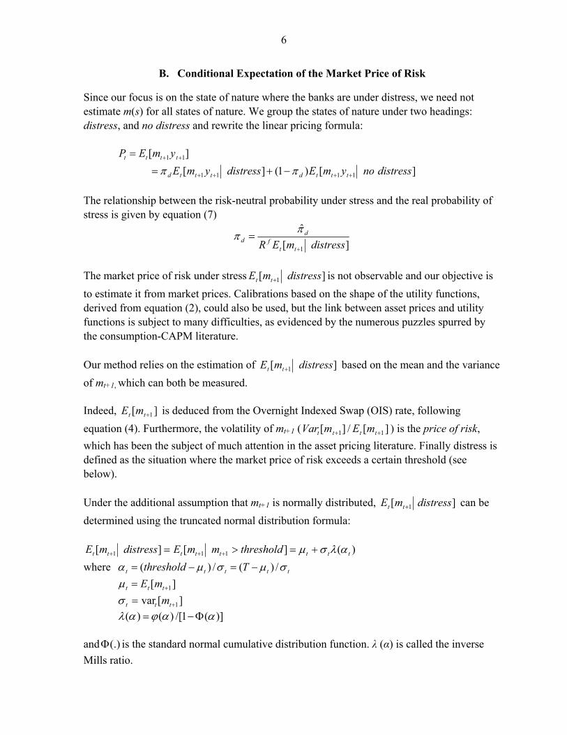
B. Conditional Expectation of the Market Price of Risk
Since our focus is on the state of nature where the banks are under distress, we need not estimate m(s) for all states of nature. We group the states of nature under two headings: distress, and no distress and rewrite the linear pricing formula:
][ 11 tttt ymEP
][)1(][ 1111 distressnoymEdistressymE tttdtttd
The relationship between the risk-neutral probability under stress and the real probability of stress is given by equation (7)
][
ˆ
1 distressmER ttf
dd
The market price of risk under stress ][ 1 distressmE tt is not observable and our objective is
to estimate it from market prices. Calibrations based on the shape of the utility functions, derived from equation (2), could also be used, but the link between asset prices and utility functions is subject to many difficulties, as evidenced by the numerous puzzles spurred by the consumption-CAPM literature. Our method relies on the estimation of ][ 1 distressmE tt based on the mean and the variance
of mt+1, which can both be measured. Indeed, ][ 1tt mE is deduced from the Overnight Indexed Swap (OIS) rate, following
equation (4). Furthermore, the volatility of mt+1 ( ][ 1tt mVar / ][ 1tt mE ) is the price of risk,
which has been the subject of much attention in the asset pricing literature. Finally distress is defined as the situation where the market price of risk exceeds a certain threshold (see below). Under the additional assumption that mt+1 is normally distributed, ][ 1 distressmE tt can be
determined using the truncated normal distribution formula:
)(][][ 111 tttttttt thresholdmmEdistressmE
where ttttt Tthreshold /)(/)(
][ 1 ttt mE
][var 1 ttt m
)](1/[)()( and (.) is the standard normal cumulative distribution function. λ (α) is called the inverse
Mills ratio.
7
We need to determine a threshold T above which banks are considered to be under stress (this threshold should ideally correspond to the states of nature where the CDS payoffs are high). We first assume, somewhat arbitrarily, that the threshold is one historical standard deviation away from the average stochastic discount factor ][ 1tt mE but we show in
section III how to extent the model so that the threshold is in line with the estimated probability of default.
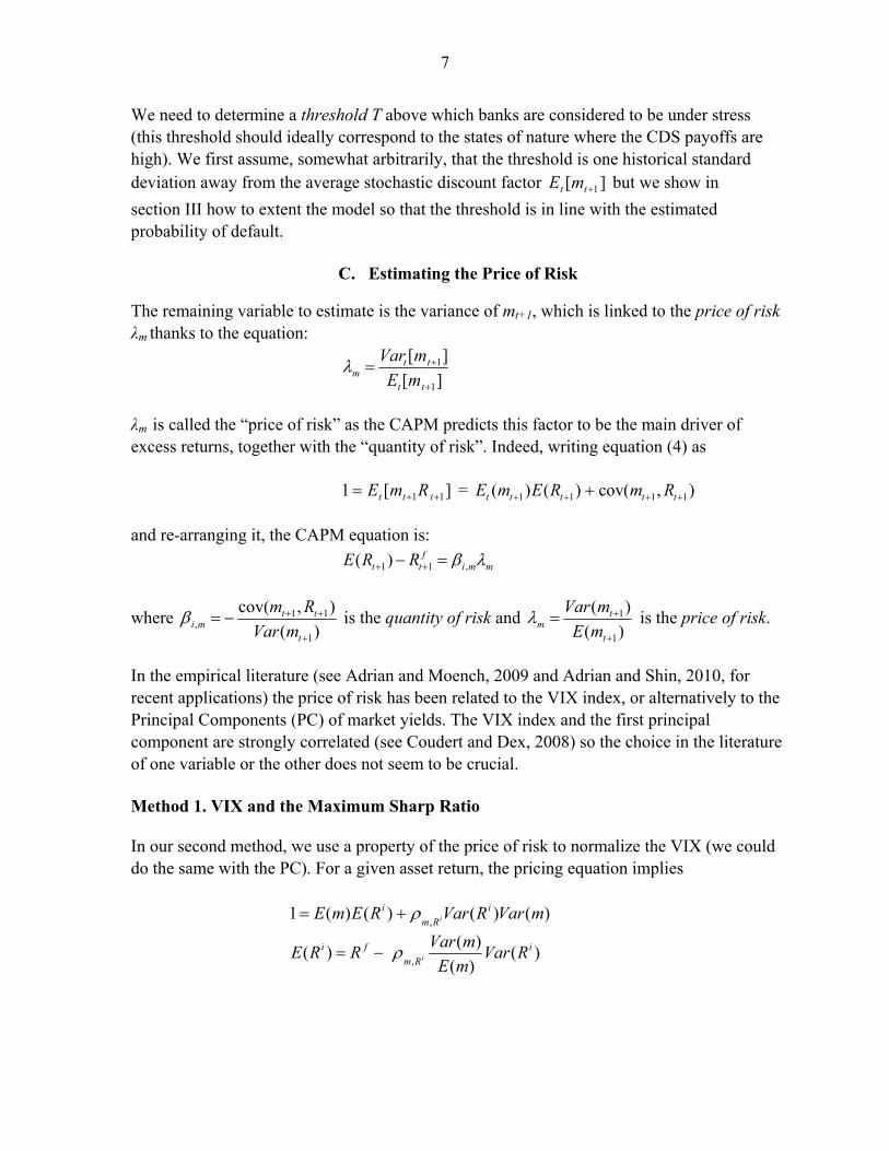
C. Estimating the Price of Risk
The remaining variable to estimate is the variance of mt+1, which is linked to the price of risk λm thanks to the equation:
][
][
1
1
tt
ttm mE
mVar
λm is called the “price of risk” as the CAPM predicts this factor to be the main driver of excess returns, together with the “quantity of risk”. Indeed, writing equation (4) as
][1 11 ttt RmE = 1 1 1 1( ) ( ) cov( , )t t t t tE m E R m R
and re-arranging it, the CAPM equation is:
1 1 ,( ) ft t i m mE R R
where )(
),cov(
1
11,
t
ttmi mVar
Rm is the quantity of risk and )(
)(
1
1
t
tm mE
mVar is the price of risk.
In the empirical literature (see Adrian and Moench, 2009 and Adrian and Shin, 2010, for recent applications) the price of risk has been related to the VIX index, or alternatively to the Principal Components (PC) of market yields. The VIX index and the first principal component are strongly correlated (see Coudert and Dex, 2008) so the choice in the literature of one variable or the other does not seem to be crucial. Method 1. VIX and the Maximum Sharp Ratio In our second method, we use a property of the price of risk to normalize the VIX (we could do the same with the PC). For a given asset return, the pricing equation implies
)()()()(1,
mVarRVarREmE i
Rm
ii
)()(
)()(
,
i
Rm
fi RVarmE
mVarRRE i

8
Since the correlation coefficient iRm, cannot be greater than 1, we deduce
)(
)(
)(
)(
mE
mVar
RVar
RREi
fi
Theoretically, the price of risk is therefore the maximum Sharpe Ratio attainable for an efficient portfolio. Historically, Sharpe ratios higher than 3 would be considered very high: we therefore decide to normalize the VIX series (by a factor of 4) in order to scale the VIX index to a series consistent with this property of the price of risk. Method 2. Principal Components and the Price of Risk We could also use the PC method proposed by Adrian and Moench (2008) to estimate the price of risk in the U.S. stock markets. Adrian and Moench (2008) applied their method to bond returns and Adrian, Etula and Shin (2010) applied it to currencies, whilst our focus is on S&P stock returns. The method relies on a CAPM equation:
, 1 1 , 1 , 1ˆ( )f
i t t i m t m tR R
where , 1ˆm t is the expected component of the market price of risk and , 1m t
is the innovation
in the market price of risk. The expected component of the market price of risk is assumed to be an affine function of the expected PC of stock market returns:
, 1 0 1 1ˆm t tPC
where 0 1, are the coefficients we need to normalize the PC to make convert it into the
estimated price of risk. If one estimates, for each asset the equation,
, 1 1 1 1 1f
i t t i i t i t tR R a b PC c PC
Adrian and Moench (2008) show that ai = βi λ0 and that βi λ1= ci, two equations that identify the normalization coefficients λ0 and λ1. They apply the model to the Principal Component of bond yields.

9
III. ENDOGENOUS THRESHOLD
The actual probability of default is deduced from the risk-neutral probability using the
formula: ))()(1(
ˆ
][)1(
ˆ
11 tttf
t
t
tttf
t
tt rTmmEr
where )](1/[)()( is the inverse Mills ratio and t
tt
T
.
The threshold T was chosen once and for all, such that 84.0][ TmP , i.e., the price of risk
under distress was one unconditional standard deviation from the unconditional mean 1/(1+ r ):
rmmET
1
1)var(*]84.0[][ 1
where 1]84.0[1 and 1 is the inverse of the cumulative normal distribution. The estimation of the market price under risk would gain in coherence if one could choose the threshold T such that the definition of the stress scenario is in line with the probability of distress that is finally estimated. This would also ensure that the threshold is bank-specific and consistent with the probability of default.
Hence, we want to set ]1[1
1)var(*]1[][ 11
rmmET
where π is the probability of default we are looking for. (Note that a very high threshold means we are looking at unlikely events, i.e., a lower π, which is why 1- π is the argument in
1 .) The probability of default therefore solves the following non-linear equation:
t
tft
tf
t
tt
rrr
]1[
1
1
1
1
)1(1
ˆ
1
(9)
or )( tt f .
10
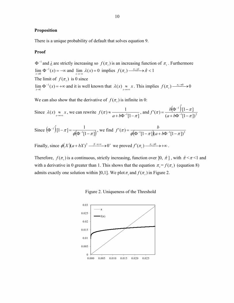
Proposition There is a unique probability of default that solves equation 9. Proof
1 and λ are strictly increasing so )( tf is an increasing function of t . Furthermore
)(lim 1
0x
xand 0)(lim
x
x implies 1ˆ)( 1 t
tf
The limit of )( tf is 0 since
)(lim 1
1x
xand it is well known that xx
x )( . This implies 0)( 0 t
tf
We can also show that the derivative of )( tf is infinite in 0:
Since xxx )( , we can rewrite
]1[
1)(
1
ba
f , and
21
1
])1[(
]1[)('
ba
bf
Since ]1[
1]1[
11
, we find 211 ])1[(]1[)('
ba
bf
Finally, since 0)( 2 XbXaX we proved 0)( t
tf .
Therefore, )( tf is a continuous, strictly increasing, function over ]0, ] , with < <1 and
with a derivative in 0 greater than 1. This shows that the equation t = )( tf (equation 8)
admits exactly one solution within ]0,1]. We plot t and )( tf in Figure 2.
Figure 2. Uniqueness of the Threshold
0
0.005
0.01
0.015
0.02
0.025
0.03
0.000 0.005 0.010 0.015 0.020 0.025
π
f(π)
11
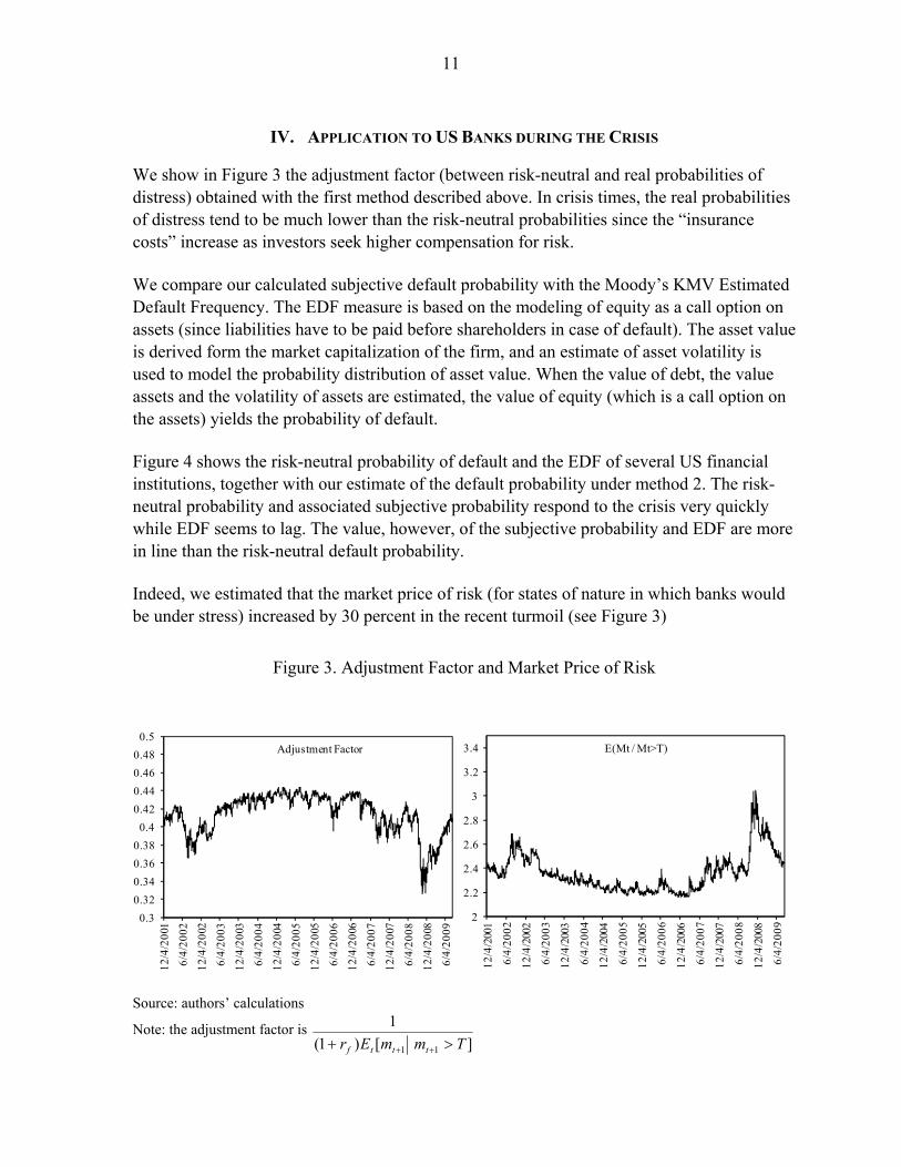
IV. APPLICATION TO US BANKS DURING THE CRISIS
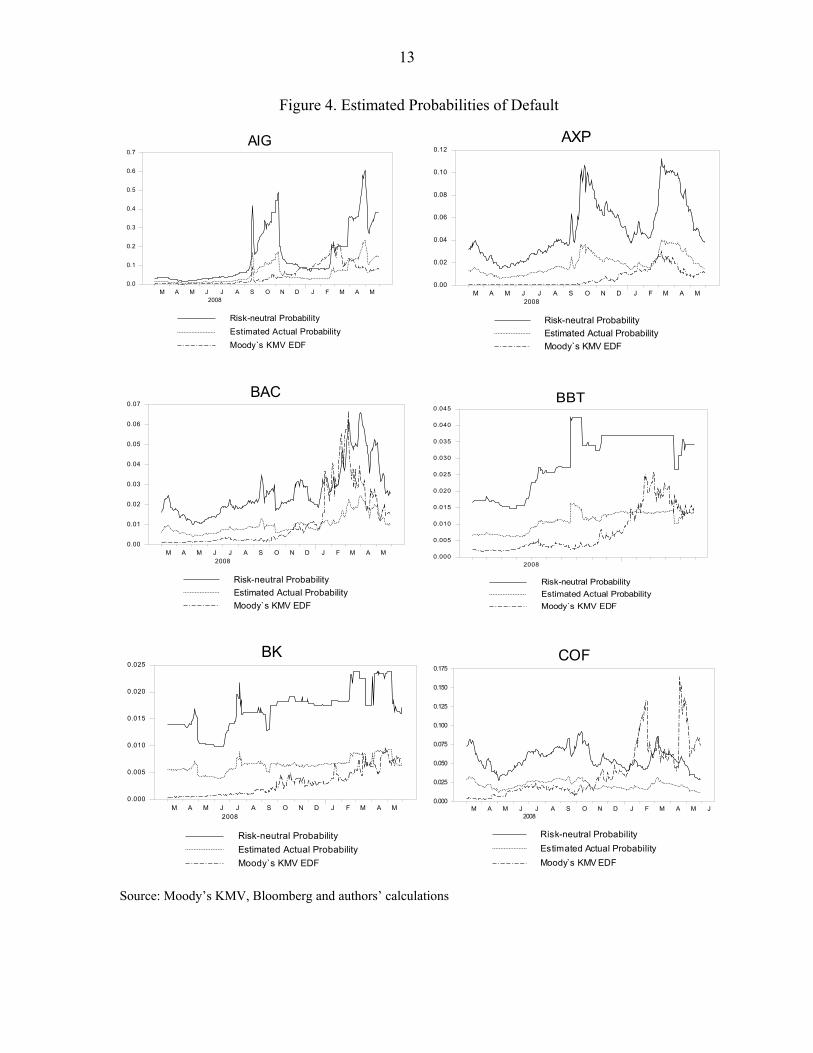
We show in Figure 3 the adjustment factor (between risk-neutral and real probabilities of distress) obtained with the first method described above. In crisis times, the real probabilities of distress tend to be much lower than the risk-neutral probabilities since the “insurance costs” increase as investors seek higher compensation for risk. We compare our calculated subjective default probability with the Moody’s KMV Estimated Default Frequency. The EDF measure is based on the modeling of equity as a call option on assets (since liabilities have to be paid before shareholders in case of default). The asset value is derived form the market capitalization of the firm, and an estimate of asset volatility is used to model the probability distribution of asset value. When the value of debt, the value assets and the volatility of assets are estimated, the value of equity (which is a call option on the assets) yields the probability of default. Figure 4 shows the risk-neutral probability of default and the EDF of several US financial institutions, together with our estimate of the default probability under method 2. The risk-neutral probability and associated subjective probability respond to the crisis very quickly while EDF seems to lag. The value, however, of the subjective probability and EDF are more in line than the risk-neutral default probability. Indeed, we estimated that the market price of risk (for states of nature in which banks would be under stress) increased by 30 percent in the recent turmoil (see Figure 3)
Figure 3. Adjustment Factor and Market Price of Risk
0.3
0.32
0.34
0.36
0.38
0.4
0.42
0.44
0.46
0.48
0.5
12/4
/200
1
6/4/
2002
12/4
/200
2
6/4/
2003
12/4
/200
3
6/4/
2004
12/4
/200
4
6/4/
2005
12/4
/200
5
6/4/
2006
12/4
/200
6
6/4/
2007
12/4
/200
7
6/4/
2008
12/4
/200
8
6/4/
2009
Adjustment Factor
2
2.2
2.4
2.6
2.8
3
3.2
3.4
12/4
/200
1
6/4/
2002
12/4
/200
2
6/4/
2003
12/4
/200
3
6/4/
2004
12/4
/200
4
6/4/
2005
12/4
/200
5
6/4/
2006
12/4
/200
6
6/4/
2007
12/4
/200
7
6/4/
2008
12/4
/200
8
6/4/
2009
E(Mt / Mt>T)
Source: authors’ calculations
Note: the adjustment factor is ][)1(
1
11 TmmEr tttf
12
V. CONCLUSION
Computing the market price of risk under situations of distress is a crucial element when one needs to use asset prices to assess probabilities of distress. We offered in this paper a simple but theoretically consistent approach to such a calculation. The approach is also free of model assumptions on the shape of the utility function, because it is based solely on an empirical one-factor model. It does not require data on past defaults and therefore is appropriate for estimating probabilities of extreme events–although it still depends on CDS market assessment of risk. We applied our method to US banks during the subprime crisis, but the method is general enough to be applied to other CDS markets. For instance, using this method, Caceres, Guizzo and Segoviano (2010) analyzed the contribution of risk aversion to the evolution of sovereign spreads in the eurozone.3 The model is based on a one-factor model but a multiple factor model would be better at fitting the data and at capturing the determinant of asset prices. The difficulty lies in matching the risk that we want to measure (the market of price of risk under a situation of distress) with the moments of the pricing factor we can observe. When several factors are assumed to determine pricing, identifying which factor to filter out requires additional understanding of the meaning of the factors and of the meaning of the risk one wants to filter out. In a one factor model, this issue does not arise. A second assumption in our method is that the price of risk is normally distributed. Relaxing this assumption may also require estimating more factors in the asset pricing model because with a one factor model, only one moment (i.e., the variance) of the price of risk can be identified. Further research is needed to generalize the method to these more complex settings.
3 Caceres, Guizzo and Segoviano (2010) showed that in the aftermath of the subprime crisis, global risk aversion and contagion factors were the main drivers behind increases in euro CDS spreads, but the turning point was in the second half of 2009, when country-specific fundamentals drove CDS in Greece, Ireland and Portugal. Another application of this method for Asia is available in Caceres and Filiz Unsal (2011).
13
Figure 4. Estimated Probabilities of Default
AIG
Risk-neutral Probability
Estimated Actual Probability
Moody`s KMV EDF
M A M J J A S O N D J F M A M2008
0.0
0.1
0.2
0.3
0.4
0.5
0.6
0.7
AXP
Risk-neutral Probability
Estimated Actual Probability
Moody`s KMV EDF
M A M J J A S O N D J F M A M2008
0.00
0.02
0.04
0.06
0.08
0.10
0.12
BAC
Risk-neutral Probability
Estimated Actual Probability
Moody`s KMV EDF
M A M J J A S O N D J F M A M2008
0.00
0.01
0.02
0.03
0.04
0.05
0.06
0.07BBT
Risk-neutral Probability
Estimated Actual Probability
Moody`s KMV EDF
20080.000
0.005
0.010
0.015
0.020
0.025
0.030
0.035
0.040
0.045
BK
Risk-neutral Probability
Estimated Actual Probability
Moody`s KMV EDF
M A M J J A S O N D J F M A M2008
0.000
0.005
0.010
0.015
0.020
0.025COF
Risk-neutral Probability
Estimated Actual Probability
Moody s KMV EDF
M A M J J A S O N D J F M A M J2008
0.000
0.025
0.050
0.075
0.100
0.125
0.150
0.175
Source: Moody’s KMV, Bloomberg and authors’ calculations
14
REFERENCES
Adrian, T., and E. Moench, 2008, “Pricing the Term Structure with Linear Regressions,” Federal Reserve Bank of New York Staff Report No. 340.
———, E. Etula, and H. Shin, 2010, “Risk Appetite and Exchange Rates,” Fed Reserve
Bank of New York Staff Report No. 361. ———, and H. Shin, 2010, “Liquidity and Leverage,” Journal of Financial Intermediation,
Vol. 19, pp. 418–437. Amato, J., 2005, “Risk Aversion and Risk Premia in the CDS Market,” BIS Quarterly
Review, December, pp. 55–68. ———, and M. Luisi, 2006, “Macro Factors in the Term Structure of Credit Spreads,” BIS
Working Paper No. 203 (Basel: Bank for International Settlements). Berndt, A., D, Rohan, D. Duffie, M. Ferguson, and D. Schranzk, 2005, “Measuring Default
Risk Premia from Default Swap Rates and EDFs,” BIS Working Paper No. 173 (Basel: Bank for International Settlements).
Black, F., and M. Scholes, 1973, “The Pricing of Options and Corporate Liabilities,” Journal
of Political Economy, Vol. 7, pp. 637–654. Caceres, C., and D., Filiz Unsal, 2011, “Sovereign Spreads and Contagion Risks in Asia,”
IMF Working paper, forthcoming. ———, V. Guzzo, and M. Segoviano, 2010, “Sovereign Spreads: Global Risk Aversion,
Contagion or Fundamentals?” IMF Working Paper 10/120 (Washington: International Monetary Fund).
Cochrane, J., 2005, Asset Pricing, Princeton NJ: Princeton University Press. Coudert V., and M. Gex, 2008, “Does Risk Aversion Drive Financial Crises? Testing the
Predictive Power of Empirical Indicators,” Journal of Empirical Finance, Vol. 15, pp. 167–184.
Jackwerth, J., 2000, “Recovering Risk Aversion from Option Prices and Realized Returns,”
Review of Financial Studies, Vol. 13, pp. 433–451. Merton R., 1974, “On the Pricing of Corporate Debt: The Risk Structure of Interest Rates,”
Journal of Finance, Vol. 29, pp. 449–470, 1974.


![[Lehman Brothers] Estimating Implied Default Probabilities From Credit Bond Prices](https://img.pdfslide.us/doc/110x75/55282fa149795917048b4613/lehman-brothers-estimating-implied-default-probabilities-from-credit-bond-prices.jpg)
