Embed Size (px)
Citation preview
1
Predictions of Default Probabilities in Structural Models of Debt
Hayne E. Leland Haas School of Business
University of California, Berkeley
April 22, 2004
The author thanks Dirk Hackbarth for his comments and invaluable assistance with the calculations and Figures. Ronald Anderson and Christopher Hennessy also provided insights and comments. An earlier version of this paper was presented at the GRETA conference “Assessing the Risk of Corporate Default”, Venice, Italy, 2002.
2
1. Introduction
This paper examines the default probabilities (DPs) that are generated by alternative “structural”
models of risky corporate bonds.1 We have three objectives:
(i) To distinguish “exogenous default” from “endogenous default” models
(ii) To compare these models’ predictions of default probabilities, given
common inputs
(iii) To examine of how well these models capture actual average default frequencies,
as reflected in Moody’s (2001) corporate bond default data 1970-2000.
.
Our analysis is limited to structural models of debt and default.2 These models assume that the
value of the firm’s activities ( “asset value”) moves randomly through time with a given expected
return and volatility. Bonds have a senior claim on the firm’s cash flow and assets. Default occurs
when the firm fails to make the promised debt service payments.
We focus on two sets of structural models that have been quite widely used in academic and/or
practical applications: those with an “exogenous default boundary” that reflects only the principal
value of debt, and those with an “endogenous default boundary” where default is chosen by
management to maximize equity value.3
1 Default probability is similar to the “expected default frequency” (EDFTM ) used by Moody’s-KMV. 2 Thus, we do not make comparisons with “reduced form” models as developed (amongst others) by Jarrow and Turnbull (1995), Jarrow, Lando, and Turnbull (1997), and Duffie and Singleton (1999). Uhrig-Homburg (2002) provides an excellent survey of both reduced form and structural models. 3 A “default boundary” is a level of asset value, perhaps time dependent, such that the firm will default on its debt if its asset value falls beneath this level. For models whose state variable is cash flow, the default boundary is a sufficiently low level of cash flow that the firm defaults on its debt.
3
Models with a default boundary that depends only upon the principal value of debt include the
pioneering work of Black and Scholes (1973) and Merton (1974). To exploit the analogy with
options, these authors restricted themselves to zero-coupon debt. With zero-coupon bonds the
default boundary is zero until the bond matures, and therefore default never occurs prior to the
bond’s maturity. At maturity, the firm defaults if asset value is less than the bond’s principal value.
Subsequent work with both endogenous and exogenous default boundaries has focused on the
default risk of coupon-paying bonds. In these models, default can occur prior to bond maturity.
Typical of recent work using an exogenous default barrier is the Longstaff and Schwartz (1995)
model (hereafter “L-S”). 4 The L-S model considers coupon-paying bonds with an exogenous
default boundary that remains constant through time. While the mathematics allows for any
constant default boundary, L-S consider a default boundary that equals the principal value of debt.
The firm defaults when asset value first falls beneath debt principal value (“negative net worth”).
However, Huang and Huang [2002] (hereafter H-H) and others have pointed out that firms often
continue to operate with negative net worth. They also note that the implied default costs must be
extremely high to explain the relatively low recovery rates on corporate bonds. H-H argue that it is
more reasonable to specify a default barrier that is some fraction β (less than or equal to one) of
debt principal.5 We shall use the L-S model, with arbitrary β, as representative of exogenous
default models. The key aspect of exogenous models is that the default barrier depends only on the
level of debt principal.
4 Other models with exogenous default include Geske [1997], Brennan and Schwartz [1980], Kim, Ramaswamy, and Sundaresan [1993], Nielsen, Saa-Requejo and Santa-Clara [1993], Briys and de Varenne [1997], and Collin-Dufresne and Goldstein [2001]. 5 For example, the Moody’s-KMV approach (which differs in some other details) postulates an exogenous default barrier that is equal to the sum of short term debt principal plus one-half of long-term debt principal (Crosbie and Bohn, [2002]). See Section 9 below.
4
An endogenous default boundary was introduced by Black and Cox [1976], and subsequently
extended by Leland [1994], Leland and Toft [1996], and Acharya and Carpenter [2002]. These
models assume that the decision to default is made by managers who act to maximize the value of
equity. At each moment, equity holders face the question: is it worth meeting promised debt
service payments? The answer depends upon whether the value of keeping equity “alive” is worth
the expense of meeting the current debt service payment.6 If the asset value exceeds the default
boundary, the firm will continue to meet debt service payments—even if asset value is less than
debt principal value, and even if cash flow is insufficient for debt service (requiring additional
equity contributions). If the asset value lies below the default boundary, it is not worth “throwing
good money after bad”: the firm does not meet the required debt service, and defaults.7, 8 In the
endogenous default model, the default boundary is that which maximizes equity value. It is
determined not only by debt principal, but also by the riskiness of the firm’s activities (as reflected
in value process), the maturity of debt issued, payout levels, default costs, and corporate tax rates.
Black and Cox [1976] and Leland [1994] derive the optimal endogenous default value for the case
of perpetual (infinite maturity) debt. Leland and Toft [1996] ( “L-T”) extend the analysis to
consider firms issuing debt of arbitrary maturity. Since they show that debt maturity affects the
default boundary and therefore default probabilities, their approach is required to calibrate the
endogenous model to empirical default data. We use the L-T model in subsequent analysis.
6 A fuller description of endogenous default is provided in Leland and Toft [1996, Section IIB]. 7 By assumption the firm is not allowed to liquidate operating assets to meet debt service payments in most structural models. Bond indentures often include covenants restricting asset sales for this purpose. 8 We presume that default occurs whenever the debt service offered is less than the amount promised. Anderson and Sundaresan (1996) and Mella-Barral and Perraudin (1996) introduce “strategic debt service”, where bargaining between equity and debtholders can lead to lesser debt service than promised, but without formal default. We do not pursue this approach here, in part because these papers assume debt with infinite maturity, whereas we focus on debt of differing maturities.
5
To capture the idea of a long-term or “permanent” capital structure, L-T presume that debt is
continuously rolled over.9 Total outstanding principal, debt service payments, and average debt
maturity, remain constant through time, even though each individual bond has a finite maturity.10
This stationary capital structure requires constant debt service payments, and the value-maximizing
default boundary is also constant through time.
The structure of the paper is as follows. Section 2 discusses some recent related empirical work.
Section 3 considers the determinants of default risk in structural models, and how they relate to
more traditional approaches to default risk. Section 4 examines how the default boundary is
determined in the exogenous and endogenous default models. Section 5 shows how cumulative
default probabilities (DPs) at different horizons are related to default boundaries and asset value
dynamics. Section 6 introduces “base case” parameters for subsequent prediction of default.
Sections 7 and 8 examine how well the L-T and L-S models match the default frequencies observed
by Moody’s (2001) over the period 1970-2000, for A-rated, Baa-rated, and B-rated debt. Section 9
shows how changes in default probabilities (and potential bond ratings) predicted by the two
approaches differ, given changes in a firm’s leverage and debt maturity. This section provides
testable hypotheses that distinguish the models. Section 10 provides a brief description of the
KMV approach. Section 11 offers some thoughts on similarities and differences between KMV,
L-S, and L-T models. Section 12 concludes.
9 To be more specific, debt is continuously offered at a maturity T, and continuously retired at par value at maturity. In the stationary case, the total principal of outstanding debt P is constant, as are the coupons C paid and the average maturity (that equals T/2). 10 As with the L-S approach, any bond issued by the firm can be readily valued in such an environment, as long as the overall capital structure is constant through time (implying the default boundary is constant through time). It is assumed that all debt issues default when the boundary is reached, consistent with the cross-default provisions that typically are included in bond covenants.
6
2. Recent Empirical Studies
Three recent papers examine related questions. Huang and Huang [2002] (“H-H”) use several
structural models, including L-S and L-T, to predict yield spreads. They calibrate inputs, including
asset volatility, for each model so that certain target variables are matched. The targets include
leverage, equity premium, recovery rate, and cumulative default probability at a single time
horizon. That horizon is 10 years in their base case, although they separately consider a 4 year
horizon. Thus inputs such as asset volatility will differ across the models H-H consider, although
they are trying to match observed default frequencies over a common time period.
H-H show that, given their calibration, the models make quite similar predictions on yield
spreads.11 Noting that empirically-observed yield spreads relative to Treasury bonds are
considerably greater than these predicted spreads (particularly for highly-rated debt), H-H conclude
that additional factors such as illiquidity and taxes must be important in explaining market yield
spreads. In contrast with H-H, we focus on predicting default probabilities rather than yield
spreads. Rather than choosing different inputs to allow the different models to match observed
default frequencies, we instead choose common inputs (including volatility) across models, to
observe how well they match observed default statistics.
In a recent paper using Merton’s [1974] approach, Cooper and Davydenko [2004] ( “C-D”) have
recently proposed a procedure somewhat the inverse of Huang and Huang [2002]. Rather than
calibrate on past default probabilities to predict (the default portion of) yield spreads, C-D propose
to predict expected default losses on any corporate bond based on its current yield spread, given
11 This is not entirely surprising. If the probability of default is similar by construction, the credit spread (involving a transformation from the actual probability process to the risk-neutral process) is likely to be similar as well.
7
information on leverage, equity volatility, and equity risk premia. To derive realistic numbers, C-D
conclude that the correct measure of a bond’s yield spread for calibrating asset volatility is not the
yield spread between that bond and a Treasury bond of similar maturity, but rather on the spread
between that bond and an otherwise-similar AAA-rated bond.
In contrast with C-D, we focus on structural models’ ability to predict the probability of default (not
the expected losses from default).12 But the C-D approach raises several interesting questions for
future research, including whether the recovery rate can potentially be untangled from the
probability of default, whether the C-D approach can be extended beyond the Merton model to
consider coupon-paying bonds, and how well the structural models that match historical default
probabilities can predict the yield spread relative to AAA-rated bonds.
Eom, Helwege, and Huang (2004) examine yield spread predictions across several structural
models. While of considerable interest for bond pricing, the work does not directly address default
probabilities.13
3. Structural Models and Default Risk
Prediction of corporate bond default rates has been an objective of financial analysis for decades.
Moody’s and Standard and Poors’ have provided bond ratings for almost a century.
12 We focus on default probability rather than expected losses not because we necessarily believe it is a more important statistic, but rather because (i) statistics are readily available on default frequencies for different bond rating classes, and (ii) it is what Standard and Poor’s claim their ratings predict (at least on a relative basis). While Moody’s empirical studies focus on their ratings’ ability to predict default frequencies, they claim that their ratings seek to explain both default frequency and loss given default. 13 Some results in the Eom et al. paper are puzzling. The average leverage, volatility, payout, and other parameters in their data set give rise to an underestimate of average yield spreads by the L-T model. This is consistent with Huang and Huang’s (2003) results. Yet Eom et al. conclude that the L-T model substantially overestimates spreads.
8
Key variables in the rating process include
Asset-liability ratios
Coverage ratios (cash flows or EBIT relative to debt service payments)
Business prospects (growth of cash flows or return on assets)
Dividends and other payouts
Business risks (volatility of cash flows or value of assets)
Asset liquidity and recovery ratios in default.
Exactly how these and perhaps other variables are balanced with one another to determine a rating
remains the proprietary information of the rating agencies. Structural models are an attempt to
create a rigorous “formula” to predict cumulative default probabilities at different horizons. Their
inputs are similar in nature to those used by ratings agencies:
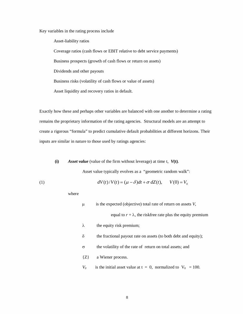
(i) Asset value (value of the firm without leverage) at time t, V(t).
Asset value typically evolves as a “geometric random walk”:
(1) ),()()(/)( tdZdttVtdV σδµ +−= 0)0( VV =
where
µ is the expected (objective) total rate of return on assets V,
equal to r + λ, the riskfree rate plus the equity premium
λ the equity risk premium;
δ the fractional payout rate on assets (to both debt and equity);
σ the volatility of the rate of return on total assets; and
{Z} a Wiener process.
V0 is the initial asset value at t = 0, normalized to V0 = 100.
9
All parameters are assumed constant through time. This modeling was introduced by Black and
Scholes [1973] and Merton [1974], and has been used in many subsequent studies.14 Note that the
total expected rate of return on assets µ is comprised of an “expected growth of asset value” rate µ -
δ, plus a “payout” rate δ on asset value.
(ii) Debt is specified by three parameters:
P the debt’s principal value
C the debt’s annual coupon flow
T the debt’s maturity.15
The coupon C is determined such that at time 0, the market value of debt D = P. Note that initial
leverage can be represented by P/V(0). While it is possible to extend both the L-S and L-T models
to consider multiple classes of debt, we consider here the case where the firm issues a single class
of debt. Note that annual debt service payments are C + P/T.
(iii) Default Boundary, VB
The default boundary is an asset value VB < V0 at which, when first reached, the firm ceases to
meet its debt service payments .16 Different structural models make different assumptions about
how VB is determined. We discuss these models in Section 4 below.
14 Zhou (2001) and Delianedis and Geske (2001) consider an asset value process with both a diffusion and a jump component. Keeping volatility constant, jumps tend to increase the default probabilities over short periods, while default probabilities over longer periods are less affected. Duffie and Lando (2001) consider the case where asset value is observed only with noise, giving results similar to models with jumps. Goldstein, Ju, and Leland (2001) postulate current cash flow or “EBIT”, rather than asset value, to be the state variable. However, because asset value is typically a fixed multiple of cash flow in these alternative models, the resulting analytics are virtually identical. Following Merton (1974) and others, we focus on models where asset value is the state variable. 15 We do not consider callable or convertible debt, though that can be considered within the context of dynamic models (e.g. Fischer, Heinkel, and Zechner (1989), Leland [1998], Goldstein, Ju, and Leland (2001), and Collin-Dufresne and Goldstein (2001)). 16 As noted previously, we ignore the possibility of “strategic debt service” as in Anderson and Sundaresan (1996) and Mella-Barral and Perraudin (1996).
10
(iv) Default Costs, α
α is the fraction of asset value VB lost when default occurs.
The fraction α lost in default is assumed to be a constant across default boundary levels.17 Costs of
default not only include the direct costs of restructuring and/or bankruptcy, but also the loss of
value resulting from employees leaving, customers directing business to other firms, trade credit
being curtailed, and the possible loss of growth options. These “indirect” costs are likely to be
several times greater than the direct costs.
Note that the recovery rate, the fraction of original principal value received by bondholders in the
event of default, is given by
(2) R = (1 - α)VB / P
The parameter α will be chosen later such that the predicted recovery rate (2) will match empirical
estimates. Loss given default (LGD) is the proportion 1 – R.
(v) Default-free interest rate, r.
We assume r , the continuously-compounded default-free interest rate, is a constant through time.18
17 Seniority is not a determinant of α here, since there is only one class of debt. 18 Kim, Ramaswamy, and Sundaresan (1993), Nielsen, Saa-Requejo and Santa-Clara (1993), Briys and de Varenne (1997), and Longstaff and Schwartz [1995] allow for stochastic default-free interest rates. A negative correlation between asset values and interest rates, as seems to accord with empirical evidence, reduces the estimated yield spreads, although the effect is quite small. Acharya and Carpenter [2002] introduce stochastic interest rates in an endogenous bankruptcy model.
11
4. The Default Boundary in Exogenous and Endogenous Cases.
4(a). Exogenous Default Boundary: The L-S Model
Recall from Section 1 the exogenous model (L-S) postulates a default barrier
(3) PV LSB β=− β ≤ 1.
Note that default boundary (3) depends only on debt principal P, and therefore is not affected by
debt maturity T, coupon rate C, firm risk σ, payout rate δ, the riskless rate r, or default costs α.
Also note from (2) that (3) implies that the recovery rate
(4) R = (1 - α)β,
and therefore the recovery rate in the L-S model is invariant to leverage as well as debt maturity,
coupon rate, firm risk, payout rate, default costs. In contrast, endogenous models typically have
recovery rates that vary with these parameters, even though α is a constant.19
4(b). Endogenous Default Boundary: The L-T Model
The L-T model assumes that the decision to default (and therefore the default boundary) is chosen
optimally by a manager maximizing equity value. To derive a constant default barrier, L-T assume
a “stationary” capital structure. Debt of a constant maturity T is continuously rolled over (unless
19 When VB is determined endogenously, as in Leland and Toft [1996], the ratio R = (1-α)VB /P tends to fall with P, implying R falls with leverage. There is some evidence suggesting a negative correlation between default rates (positively related to leverage) and recovery ratios: see Altman et al. (2001) and Bakshi, Madan, and Zhang (2001). However, this may also reflect seniority differences.
12
default occurs). As debt matures, it is replaced by new debt with equal principal value and
maturity. Total debt principal will be constant at a level P, with coupon flow C. Although the
firm has an aggregate debt structure that is presumed stationary, any particular bond can be valued
as in L-S, but with the default barrier VB-LT used for valuation rather than the default barrier VB-LS.
The optimal default boundary in L-T is given by the (complex) formula
(5) Bx
rCxrTAPBrTArCV LTB )1(1/)/())/)(/(
αατ
−−+−−−
=− ,
where the variables A and B are defined in the Appendix. C is the coupon that results in the bond
selling initially at par, n[•] and N[•] denote the standard normal density and cumulative distribution
functions, respectively, and τ is the corporate income tax rate. Note that, like bond prices, VB-LT
depends only the risk-neutral drift r and not on the actual drift µ.
The default boundary VB-LT decreases with maturity T, volatility σ, and the riskfree rate r, increases
with default costs α and increases more than proportionately with principal P.
5. The Default Probability (DP) with Constant Default Barrier
With a constant default barrier, the mathematics of European-style barrier options are applicable.
The first-passage time probability density function for reaching a barrier VB at time t from a
starting value V0 > VB is given by
13
(6) )2/())5.((
3
22
2),,,;( ttbe
t
bbtf σσδµ
σσδµ −−+−
⎟⎟⎠
⎞⎜⎜⎝
⎛
Π=
where )./( 0 BVVLnb =
The first-passage time cumulative probability function determines the cumulative default
probability (DP) at time t:
(7) ]/))5.([(]/))5.([(),,,;( 2/)5.(22 22
ttbNettbNbtDP b σσδµσσδµσδµ σσδµ −−+−+−−−−= −−− .
In the Merton (1974) model, default never occurs before the zero-coupon bond matures at T. At T,
VB = P and the probability of default is
(8) ]/))5.([( 2 TTbN σσδµ −−−− .20
It is obvious that (8) is always less than (7) at t = T. Since the default boundary in the Merton
model is zero for all t until T, default is always less likely in the Merton model than the constant
default barrier model with VB = P.
6. Calibration of Models: The Base Case
We follow Huang and Huang (2002) in many of our parameter choices, focusing on debt with a
Baa rating. Base case parameters are:
20 Note that the argument of (8) is the same as (negative) “d2” in the Black-Scholes option pricing formula with proportional dividends δ, but with the actual drift µ replacing the risk-neutral drift r.
14
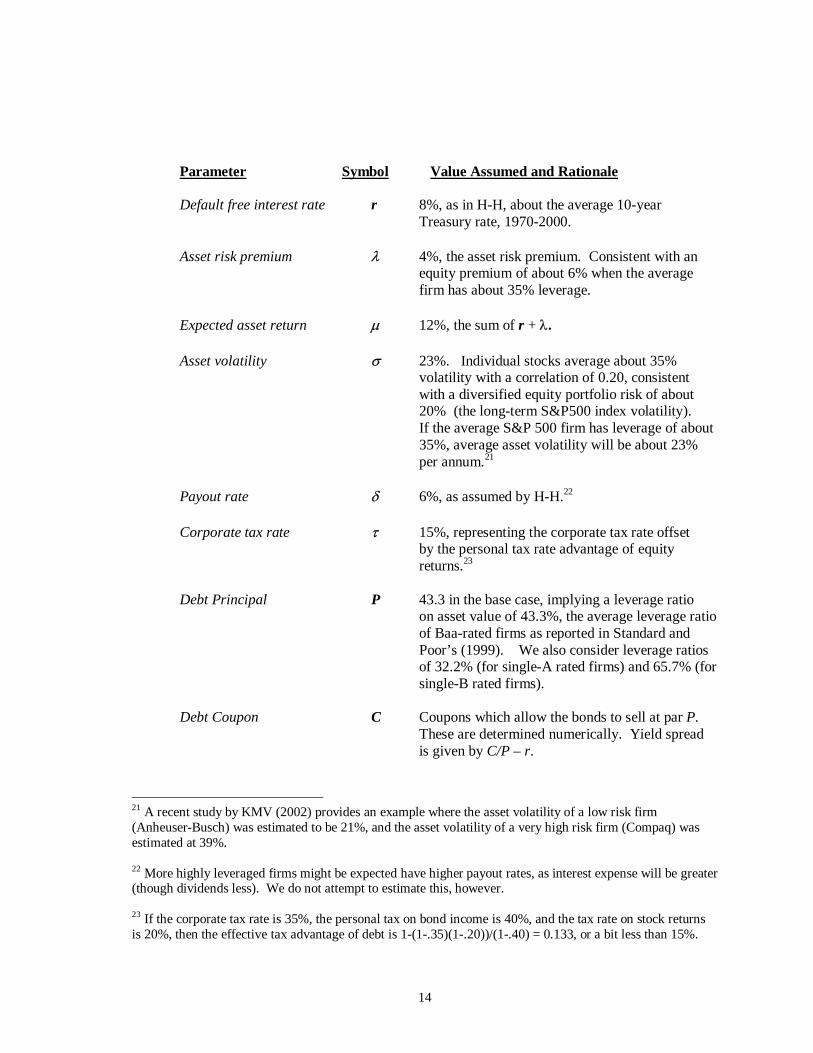
Parameter Symbol Value Assumed and Rationale
Default free interest rate r 8%, as in H-H, about the average 10-year Treasury rate, 1970-2000.
Asset risk premium λ 4%, the asset risk premium. Consistent with an equity premium of about 6% when the average firm has about 35% leverage.
Expected asset return µ 12%, the sum of r + λ.
Asset volatility σ 23%. Individual stocks average about 35% volatility with a correlation of 0.20, consistent with a diversified equity portfolio risk of about 20% (the long-term S&P500 index volatility). If the average S&P 500 firm has leverage of about 35%, average asset volatility will be about 23% per annum.21
Payout rate δ 6%, as assumed by H-H.22
Corporate tax rate τ 15%, representing the corporate tax rate offset by the personal tax rate advantage of equity
returns.23
Debt Principal P 43.3 in the base case, implying a leverage ratio on asset value of 43.3%, the average leverage ratio of Baa-rated firms as reported in Standard and Poor’s (1999). We also consider leverage ratios of 32.2% (for single-A rated firms) and 65.7% (for single-B rated firms).
Debt Coupon C Coupons which allow the bonds to sell at par P. These are determined numerically. Yield spread is given by C/P – r.
21 A recent study by KMV (2002) provides an example where the asset volatility of a low risk firm (Anheuser-Busch) was estimated to be 21%, and the asset volatility of a very high risk firm (Compaq) was estimated at 39%. 22 More highly leveraged firms might be expected have higher payout rates, as interest expense will be greater (though dividends less). We do not attempt to estimate this, however. 23 If the corporate tax rate is 35%, the personal tax on bond income is 40%, and the tax rate on stock returns is 20%, then the effective tax advantage of debt is 1-(1-.35)(1-.20))/(1-.40) = 0.133, or a bit less than 15%.
15
Maturity T 10 years in the base case. We also consider bond maturities of 5 and 20 years.24
Fractional default costs α 30%, which will imply a 51% recovery rate in the base case, the recovery rate assumed by H-H.25
7. Matching Empirical Default Frequencies with the L-T Model
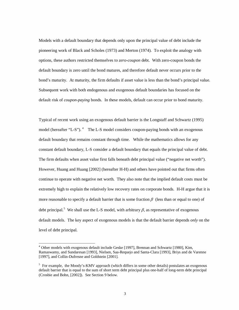
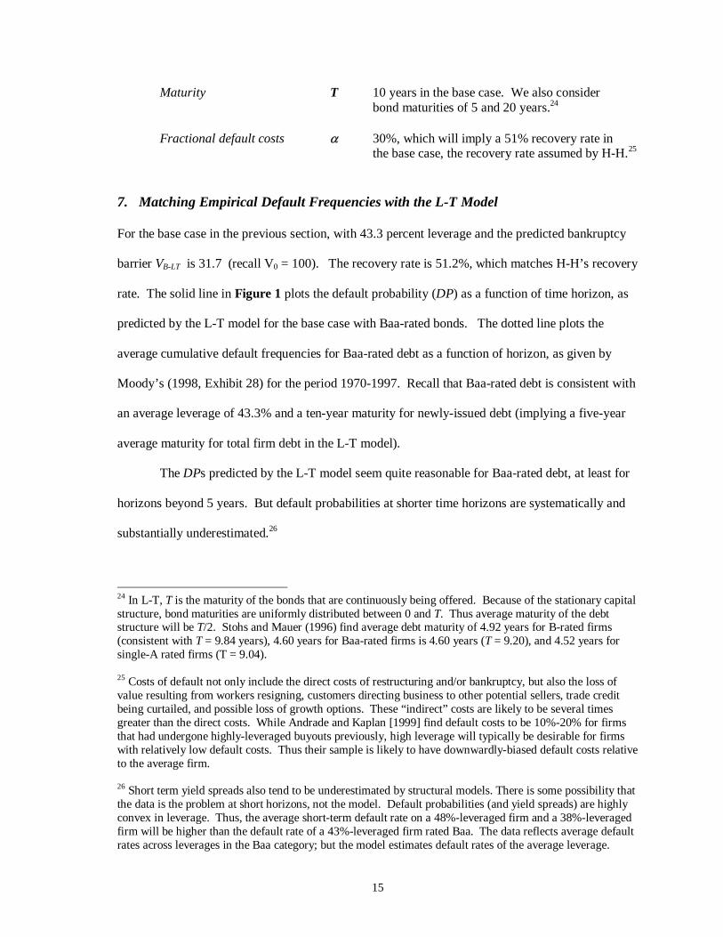
For the base case in the previous section, with 43.3 percent leverage and the predicted bankruptcy
barrier VB-LT is 31.7 (recall V0 = 100). The recovery rate is 51.2%, which matches H-H’s recovery
rate. The solid line in Figure 1 plots the default probability (DP) as a function of time horizon, as
predicted by the L-T model for the base case with Baa-rated bonds. The dotted line plots the
average cumulative default frequencies for Baa-rated debt as a function of horizon, as given by
Moody’s (1998, Exhibit 28) for the period 1970-1997. Recall that Baa-rated debt is consistent with
an average leverage of 43.3% and a ten-year maturity for newly-issued debt (implying a five-year
average maturity for total firm debt in the L-T model).
The DPs predicted by the L-T model seem quite reasonable for Baa-rated debt, at least for
horizons beyond 5 years. But default probabilities at shorter time horizons are systematically and
substantially underestimated.26
24 In L-T, T is the maturity of the bonds that are continuously being offered. Because of the stationary capital structure, bond maturities are uniformly distributed between 0 and T. Thus average maturity of the debt structure will be T/2. Stohs and Mauer (1996) find average debt maturity of 4.92 years for B-rated firms (consistent with T = 9.84 years), 4.60 years for Baa-rated firms is 4.60 years (T = 9.20), and 4.52 years for single-A rated firms (T = 9.04). 25 Costs of default not only include the direct costs of restructuring and/or bankruptcy, but also the loss of value resulting from workers resigning, customers directing business to other potential sellers, trade credit being curtailed, and possible loss of growth options. These “indirect” costs are likely to be several times greater than the direct costs. While Andrade and Kaplan [1999] find default costs to be 10%-20% for firms that had undergone highly-leveraged buyouts previously, high leverage will typically be desirable for firms with relatively low default costs. Thus their sample is likely to have downwardly-biased default costs relative to the average firm. 26 Short term yield spreads also tend to be underestimated by structural models. There is some possibility that the data is the problem at short horizons, not the model. Default probabilities (and yield spreads) are highly convex in leverage. Thus, the average short-term default rate on a 48%-leveraged firm and a 38%-leveraged firm will be higher than the default rate of a 43%-leveraged firm rated Baa. The data reflects average default rates across leverages in the Baa category; but the model estimates default rates of the average leverage.
16
FIGURE 1
0 5 10 15 20Default Horizon in Years
0
0.02
0.04
0.06
0.08
0.1
PD:
0791-
0002
43.3 % Leverage and 10- Year Maturity
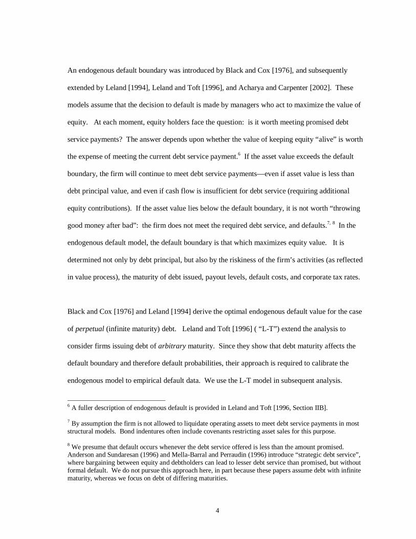
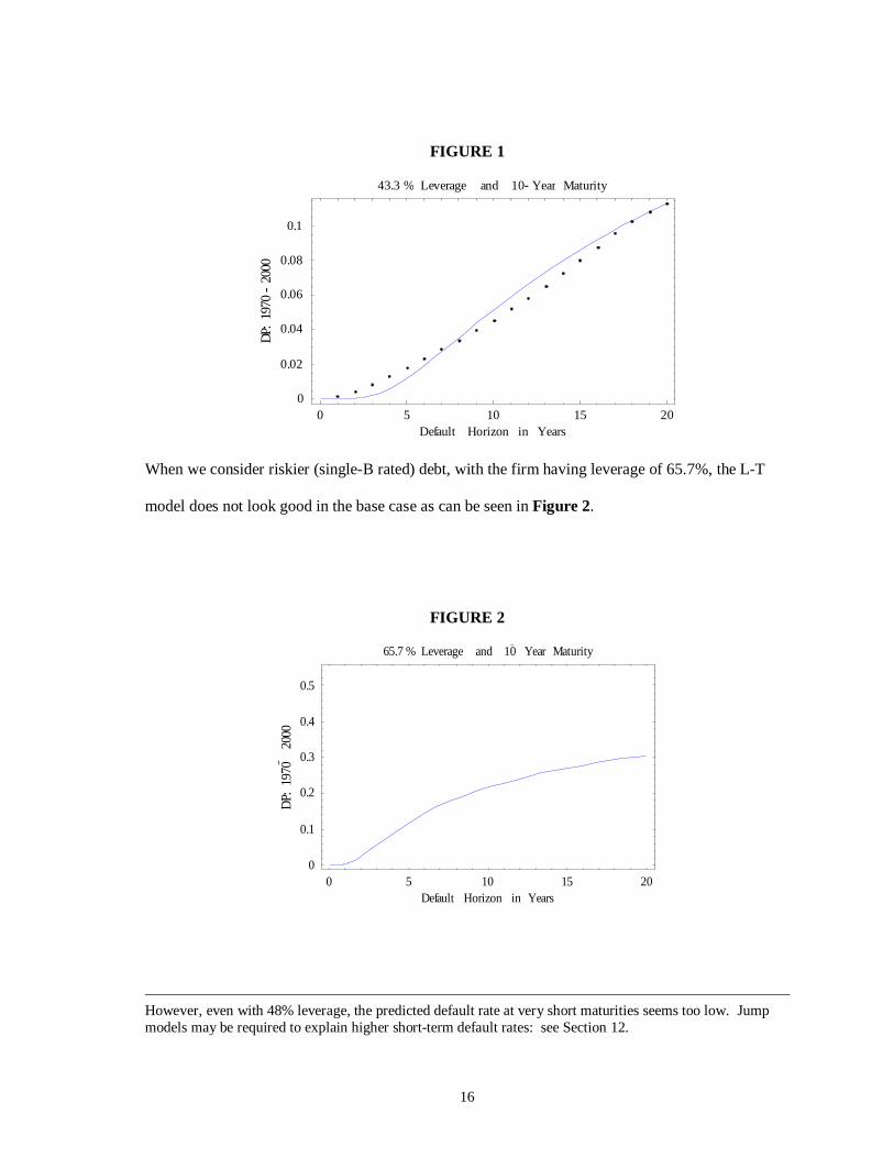
When we consider riskier (single-B rated) debt, with the firm having leverage of 65.7%, the L-T
model does not look good in the base case as can be seen in Figure 2.
FIGURE 2
0 5 10 15 20Default Horizon in Years
0
0.1
0.2
0.3
0.4
0.5
PD:
0791
0002
65.7 % Leverage and 10 Year Maturity
However, even with 48% leverage, the predicted default rate at very short maturities seems too low. Jump models may be required to explain higher short-term default rates: see Section 12.
17
The actual default probabilities are considerably higher for all default horizons than predicted by
the L-T approach. But there is no reason to think that the base case—which was predicated on the
volatility of a typical firm—is relevant to firms issuing B-rated debt.
While Stohs and Mauer (1996) show that B-rated debt has about the same average maturity as Baa-
rated debt, there is reason to believe that the firms with B-rated debt have higher asset volatility.
Unfortunately, publicly-available data that links firm volatility to initial debt rating is unavailable.
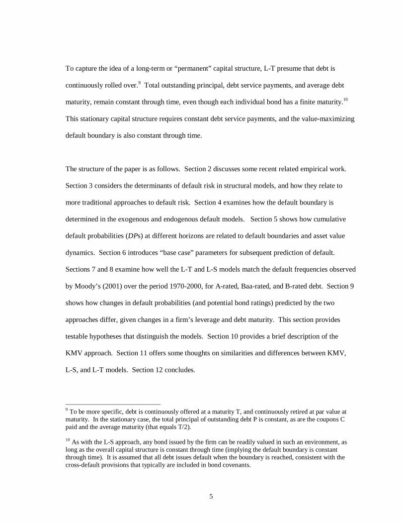
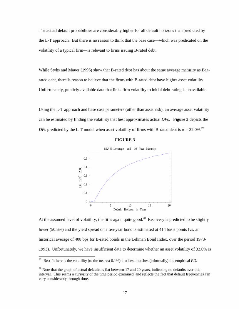
Using the L-T approach and base case parameters (other than asset risk), an average asset volatility
can be estimated by finding the volatility that best approximates actual DPs. Figure 3 depicts the
DPs predicted by the L-T model when asset volatility of firms with B-rated debt is σ = 32.0%.27
FIGURE 3
0 5 10 15 20Default Horizon in Years
0
0.1
0.2
0.3
0.4
0.5
PD:
0791
0002
65.7 % Leverage and 10 Year Maturity
At the assumed level of volatility, the fit is again quite good.28 Recovery is predicted to be slightly
lower (50.6%) and the yield spread on a ten-year bond is estimated at 414 basis points (vs. an
historical average of 408 bps for B-rated bonds in the Lehman Bond Index, over the period 1973-
1993). Unfortunately, we have insufficient data to determine whether an asset volatility of 32.0% is 27 Best fit here is the volatility (to the nearest 0.1%) that best matches (informally) the empirical PD. 28 Note that the graph of actual defaults is flat between 17 and 20 years, indicating no defaults over this interval. This seems a curiosity of the time period examined, and reflects the fact that default frequencies can vary considerably through time.
18
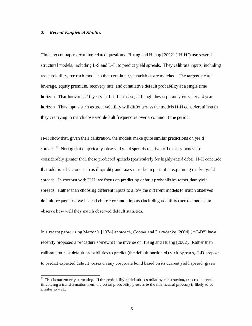
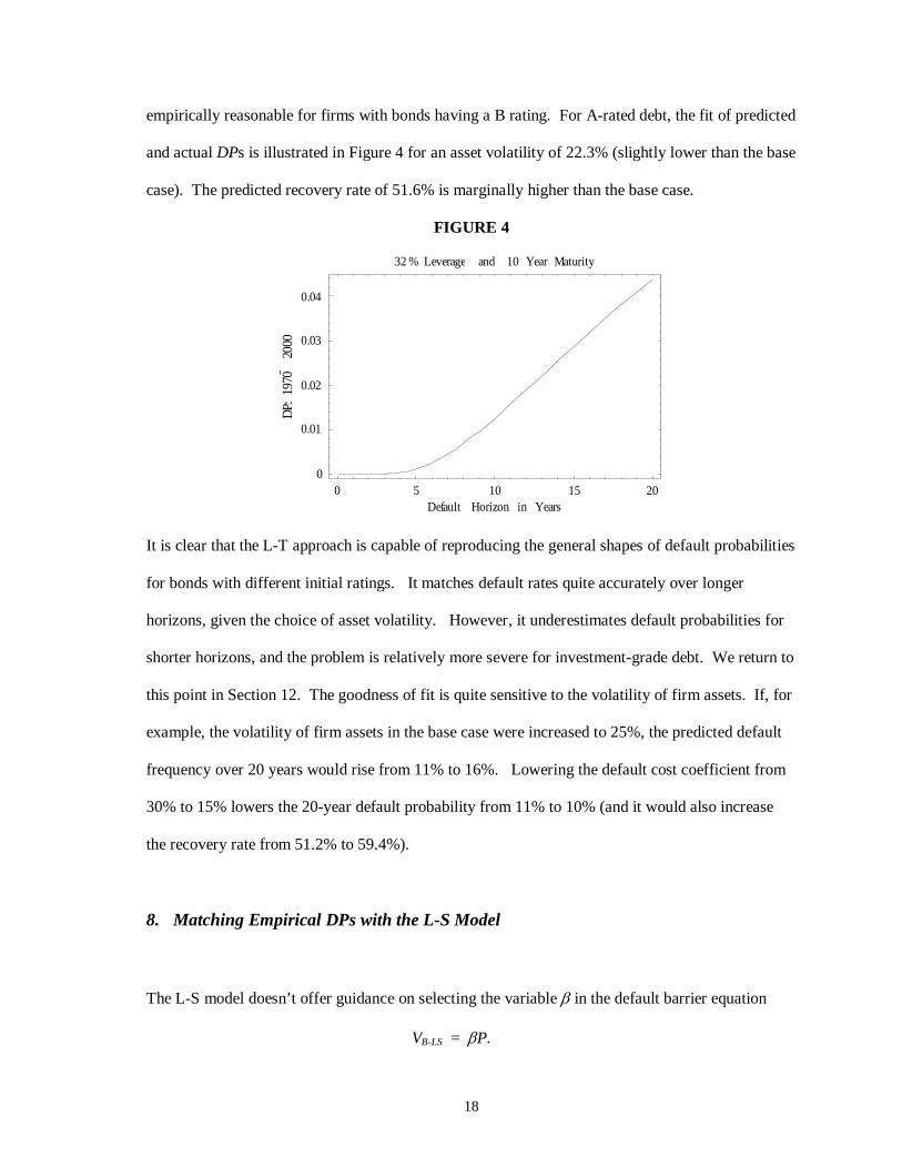
empirically reasonable for firms with bonds having a B rating. For A-rated debt, the fit of predicted
and actual DPs is illustrated in Figure 4 for an asset volatility of 22.3% (slightly lower than the base
case). The predicted recovery rate of 51.6% is marginally higher than the base case.
FIGURE 4
0 5 10 15 20Default Horizon in Years
0
0.01
0.02
0.03
0.04PD:
0791
0002
32 % Leverage and 10 Year Maturity
It is clear that the L-T approach is capable of reproducing the general shapes of default probabilities
for bonds with different initial ratings. It matches default rates quite accurately over longer
horizons, given the choice of asset volatility. However, it underestimates default probabilities for
shorter horizons, and the problem is relatively more severe for investment-grade debt. We return to
this point in Section 12. The goodness of fit is quite sensitive to the volatility of firm assets. If, for
example, the volatility of firm assets in the base case were increased to 25%, the predicted default
frequency over 20 years would rise from 11% to 16%. Lowering the default cost coefficient from
30% to 15% lowers the 20-year default probability from 11% to 10% (and it would also increase
the recovery rate from 51.2% to 59.4%).
8. Matching Empirical DPs with the L-S Model
The L-S model doesn’t offer guidance on selecting the variable β in the default barrier equation
VB-LS = βP.
19
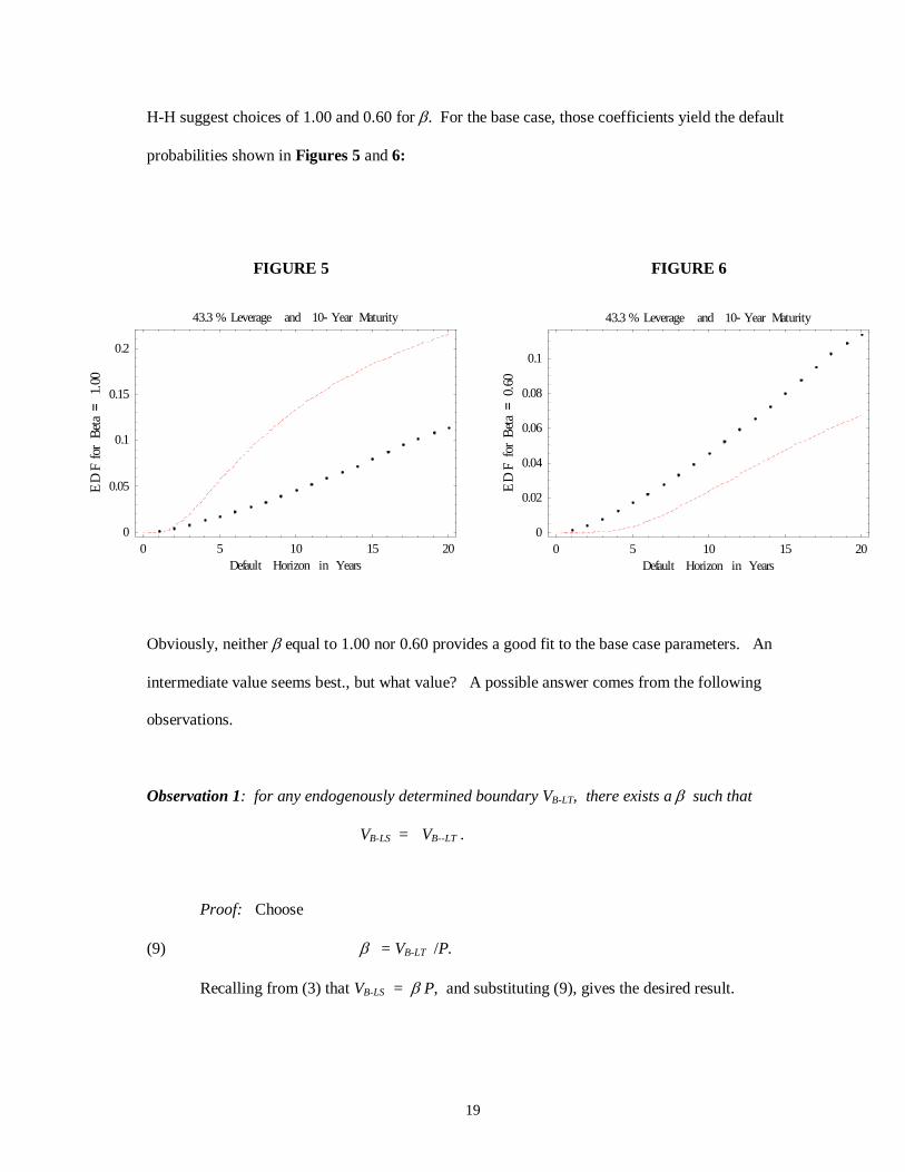
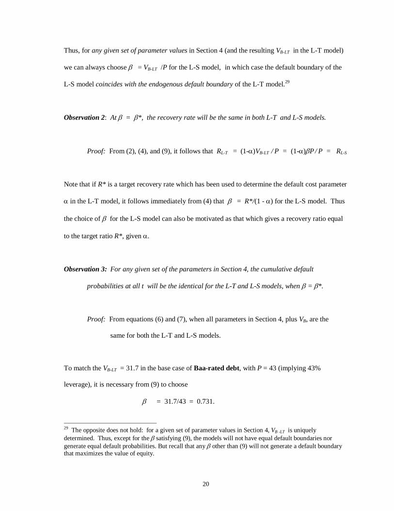
H-H suggest choices of 1.00 and 0.60 for β. For the base case, those coefficients yield the default
probabilities shown in Figures 5 and 6:
FIGURE 5 FIGURE 6
Obviously, neither β equal to 1.00 nor 0.60 provides a good fit to the base case parameters. An
intermediate value seems best., but what value? A possible answer comes from the following
observations.
Observation 1: for any endogenously determined boundary VB-LT, there exists a β such that
VB-LS = VB--LT .
Proof: Choose
(9) β = VB-LT /P.
Recalling from (3) that VB-LS = β P, and substituting (9), gives the desired result.
0 5 10 15 20Default Horizon in Years
0
0.05
0.1
0.15
0.2
ED
Frof
ateB=
00.1
43.3 % Leverage and 10- Year Maturity
0 5 10 15 20Default Horizon in Years
0
0.02
0.04
0.06
0.08
0.1
ED
Frof
ateB=
06.0
43.3 % Leverage and 10- Year Maturity
20
Thus, for any given set of parameter values in Section 4 (and the resulting VB-LT in the L-T model)
we can always choose β = VB-LT /P for the L-S model, in which case the default boundary of the
L-S model coincides with the endogenous default boundary of the L-T model.29
Observation 2: At β = β*, the recovery rate will be the same in both L-T and L-S models.
Proof: From (2), (4), and (9), it follows that RL-T = (1-α)VB-LT / P = (1-α)βP / P = RL-S
Note that if R* is a target recovery rate which has been used to determine the default cost parameter
α in the L-T model, it follows immediately from (4) that β = R*/(1 - α) for the L-S model. Thus
the choice of β for the L-S model can also be motivated as that which gives a recovery ratio equal
to the target ratio R*, given α.
Observation 3: For any given set of the parameters in Section 4, the cumulative default
probabilities at all t will be the identical for the L-T and L-S models, when β = β*.
Proof: From equations (6) and (7), when all parameters in Section 4, plus VB, are the
same for both the L-T and L-S models.
To match the VB-LT = 31.7 in the base case of Baa-rated debt, with P = 43 (implying 43%
leverage), it is necessary from (9) to choose
β = 31.7/43 = 0.731.
29 The opposite does not hold: for a given set of parameter values in Section 4, VB -LT is uniquely determined. Thus, except for the β satisfying (9), the models will not have equal default boundaries nor generate equal default probabilities. But recall that any β other than (9) will not generate a default boundary that maximizes the value of equity.
21
By the construction of this β , both models have the same default boundary and recovery ratios in
the base case for Baa-rated bonds. Thus the DP graph for the L-S model is identical to that of the
L-T model in Figure 1. We use β = 0.731 in comparing the default probability predictions of the
exogenous (L-S) and endogenous (L-T) default model for B-rated and A-rated bonds.
While the L-S model can always replicate the DP curves produced by the L-T model, the opposite
is note true. The L-S model potentially has more flexibility to fit the data than the L-T model. For
example, any combination of (1 - α)β for the L-S model generates a 51.2% recovery rate and thus
will fit the recovery data equally well.30 The combination (α = 14.7%, β = 0.60) generates the
same recovery rate, using a default cost number which some studies might suggest is more
reasonable than α = 0.30. But such a combination yields very poor predictions of default
probabilities: see Figure 6, which examines exactly this case. Indeed, the best fit of default
probabilities for the L-S model (given the parameters excluding α) is when α = 0.30 and β = 0.731.
With σ = 23%, the L-S model (like the L-T model) underestimates the DPs for B-rated debt,
where leverage is 65.7 percent. Raising asset volatility to 32% produces an almost-identical fit,
when β = 0.731. The L-S default curve is very slightly higher than the L-T default curve in Figure
3, but it is not reproduced separately since the curves are practically indistinguishable. The DP
curves are similar because the endogenous recovery ratio in the L-T model remains remain virtually
unchanged from the base case (50.7% vs. 51.2%), despite the increase in volatility and greater
leverage of B-rated firms. The equilibrating VB-LS would require β = R / (1 - α) = .507 / 0.70 =
0.724, which is very close to 0.731. It is impossible to claim one of these is superior to the other,
since the default probability curves are virtually identical, and the empirical cumulative default
30 Recall α = 0.30 was required in the L-T model to generate the observed recovery rate of 51.2%.
22
frequencies have considerable dispersion about their average.31
A similar situation arises for A-rated debt, where leverage averages 32%. At an asset volatility of
22.3%, fractionally lower than the base case, both the L-S model with β = 0.731 and the L-T
model again predict almost the same default probabilities. Matching the L-S model’s
endogenously-determined recovery rate of 51.6% for A-rated debt would require β = R / (1 - α) =
0.516/ 0.70 = 0.737. Retaining β = 0 .731 results in insignificant differences in default
probabilities between the exogenous and endogenous models.
Other differences in the models’ predictions, however, are potentially testable. For example, the
endogenous (L-T) default boundary falls with asset volatility or with debt maturity, ceteris paribus,
and thus the model predicts that recovery ratios decline with higher firm risk or with greater debt
maturity. The exogenous (L-S) model predicts no change in the recovery rate or default frequency
as these variables change.
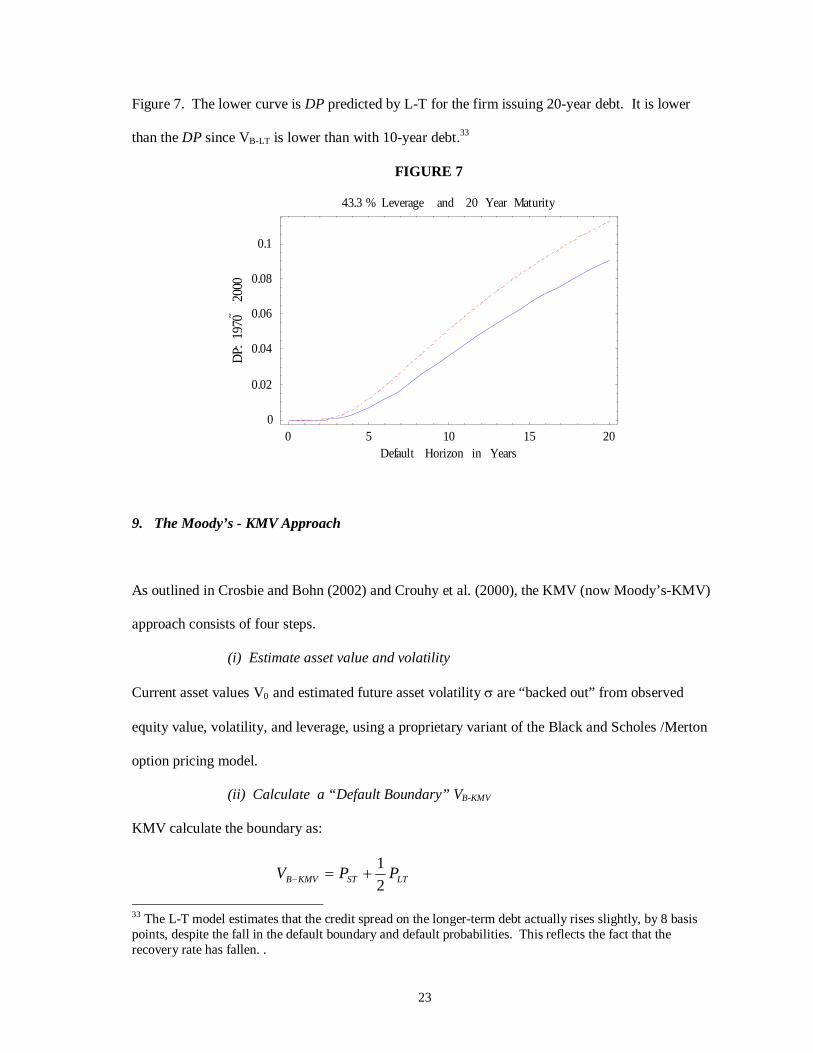
We consider the case where a firm (with Baa-rated debt in the base case) wishes to issue 20-year
debt rather than 10-year debt. Figure 7 shows the cumulative default probabilities predicted by the
two models. The L-S model predicts no change in the default probability curve (the higher dashed
line), since the exogenous default boundary is invariant to maturity.32 This is the upper curve in
31 Recall the average cumulative default frequency (over 1970-2000) after t years is the average of the cumulative default frequencies of different cohorts of bonds of a given rating, t years after issuance. The default histories of different cohorts have considerable variability: See Moody’s [2001]. 32 If it is argued that β should change with bond maturity, it is necessary to specify how. The L-S model does not provide an answer, although the L-T model implies one.
23
Figure 7. The lower curve is DP predicted by L-T for the firm issuing 20-year debt. It is lower
than the DP since VB-LT is lower than with 10-year debt.33
FIGURE 7
0 5 10 15 20Default Horizon in Years
0
0.02
0.04
0.06
0.08
0.1PD:
0791
0002
43.3 % Leverage and 20 Year Maturity
9. The Moody’s - KMV Approach
As outlined in Crosbie and Bohn (2002) and Crouhy et al. (2000), the KMV (now Moody’s-KMV)
approach consists of four steps.
(i) Estimate asset value and volatility
Current asset values V0 and estimated future asset volatility σ are “backed out” from observed
equity value, volatility, and leverage, using a proprietary variant of the Black and Scholes /Merton
option pricing model.
(ii) Calculate a “Default Boundary” VB-KMV
KMV calculate the boundary as:
LTSTKMVB PPV21
+=−
33 The L-T model estimates that the credit spread on the longer-term debt actually rises slightly, by 8 basis points, despite the fall in the default boundary and default probabilities. This reflects the fact that the recovery rate has fallen. .
24
where PST is the principal of short term liabilities and PLT the principal of long term liabilities. It
appears that KMV considers a liability to be “short term” if it is due within the horizon t over which
the default probability is computed. Longer horizons thus have a higher fraction of “short term”
liabilities, with a consequent higher default barrier.34
A special case of interest is a “rolled over” capital structure similar to L-T, with constant total debt
P and equal amounts P/T of each maturity debt, 1,..,T. If the default horizon is t years, then
(10)
( )
PT
TtMin
PT
TtMinPT
TtMinTtV KMVB
⎟⎠
⎞⎜⎝
⎛⎟⎠⎞
⎜⎝⎛⎟⎠⎞
⎜⎝⎛+=
−+=−
),(21
21
)),(1(21,),(
The KMV default boundary depends on the debt maturity T. But unlike either L-S or L-T, the
KMV boundary also depends upon time t. Therefore equation (7) does not apply.
(iii) Calculate the Distance to Default (DD)
DD(t) is measured by number of standard deviations between the (log of) the ratio of the expected
future asset level V(t) (given V0), and the KMV default boundary at t., using the current asset level
V0 and asset return volatility σ estimated in step (i). This is given by
(11) t
ttV
VLn
tDD KMVB
σ
σδµ ))5.())(
()(
20 −−−= −
where we have suppressed the argument T in VB-KMV (t, T).
34 Recall that both the L-S and L-T models have a constant default barrier, although dynamic variants may have VB upwardly-ratcheted (on average) with time. See, for example, Leland [1998] and Goldstein, Ju, and Leland [2001].
25
(iv) Map DD(t) into DP(t).
KMV has an extensive proprietary data base relating firms’ empirical cumulative default
frequencies t periods in the future to estimated DD(t) and t. It thus creates a mapping f such that
the default probability (termed EDF, expected default frequency) is:
(12) EDF(t) = DP(t) = f (DD(t), t).
This DP(t) can then be compared with the actual average default frequencies of bonds with
different ratings, to derive an “implicit” bond rating. In their publicly-available papers, KMV show
that if asset values followed the diffusion process (1), then their DP at horizon t will be given by
(13) DP(t) = )]([ tDDN − ,
where N(•) is the standard normal cumulative distribution function.35 Note that (13) is simply the
default probability for a zero-coupon bond with maturity t and principal VB-KMV (t,T) that is given in
equation (10). This links KMV’s approach with Merton (1974).
10. Some Preliminary Thoughts on the Relationship Between the KMV Approach and L-S/L-T
Given the VB-KMV(t,T) function as in equation (10), and that asset values follow the diffusion
process in equation (1), we can compute KMV’s DP(t) from equation (12).
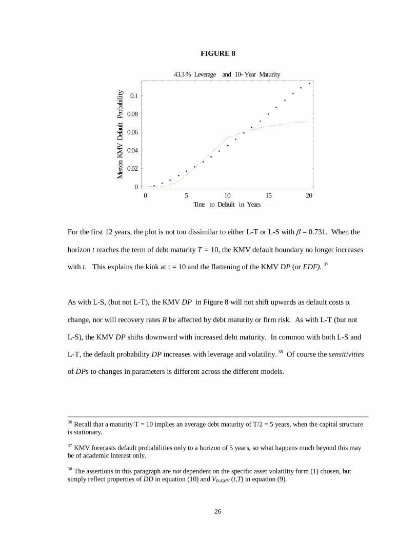
Figure 8 plots the DP as a function of horizon t for the base case:36
35 We stress that KMV does not necessarily believe that asset values follow the diffusion process (1), although they use it for illustrative purposes. We nonetheless use it to compare the differences in default probability estimates that the various approaches would make under the same set of assumptions about asset value movements.
26
FIGURE 8
For the first 12 years, the plot is not too dissimilar to either L-T or L-S with β = 0.731. When the
horizon t reaches the term of debt maturity T = 10, the KMV default boundary no longer increases
with t. This explains the kink at t = 10 and the flattening of the KMV DP (or EDF). 37
As with L-S, (but not L-T), the KMV DP in Figure 8 will not shift upwards as default costs α
change, nor will recovery rates R be affected by debt maturity or firm risk. As with L-T (but not
L-S), the KMV DP shifts downward with increased debt maturity. In common with both L-S and
L-T, the default probability DP increases with leverage and volatility. 38 Of course the sensitivities
of DPs to changes in parameters is different across the different models.
36 Recall that a maturity T = 10 implies an average debt maturity of T/2 = 5 years, when the capital structure is stationary. 37 KMV forecasts default probabilities only to a horizon of 5 years, so what happens much beyond this may be of academic interest only. 38 The assertions in this paragraph are not dependent on the specific asset volatility form (1) chosen, but simply reflect properties of DD in equation (10) and VB-KMV (t,T) in equation (9).
0 5 10 15 20Time to Default in Years
0
0.02
0.04
0.06
0.08
0.1
notreM�VMK
tluafeDytilibaborP
43.3 % Leverage and 10-Year Maturity
27
At a more conceptual level, having the distance-to-default DD(t) as the sole argument in KMV’s
DP (whether through (13) or a more general relationship (12)) is a strong restriction. Observe that
equation (13) gives the probability of being beneath VB-KMV (t) at the horizon t only, and not the
probability of falling beneath the barrier VB-KMV (τ) at any time τ within the horizon [0, t]. This is in
contrast with L-S and L-T, where the argument for DP is given by equation (7). That equation has
DD as the first term in its argument, but has a second term as well. This implies that DD is not a
sufficient statistic for DP in equation (7), and that ordinal rankings of the two criteria can differ.
For example, at longer horizons, the DD(t) as computed in equation (13) can decline with t –i.e. the
estimated default frequency can actually decrease with a longer horizon, even though this should
not be possible for a cumulative default probability function. For the base case, the KMV DP is
decreasing with the time horizon when t exceeds 25 years.39
12. Conclusions
We have compared structural models’ abilities to predict observed default rates on corporate bonds.
The endogenous L-T model derives a constant default boundary that optimizes equity value. The
exogenous L-S model assumes a constant default boundary through time, at a level equal to an
exogenously-specified fraction β of debt principal value. β = 1 (a positive net worth condition) is
a logical choice for this parameter, but gives poor predictions of default probabilities and recovery
rates. Thus, we consider β a free parameter for the exogenous model.
When β can be chosen freely, the exogenous model can always replicate the endogenous model’s
default predictions, but not vice-versa. However, we found that the β which equates the models’
defaults predictions is in fact the best choice to explain observed default rates for the period 1970-
39 Because KMV limits forecasts of EDFs to 5 years, this is a theoretical but not a practical difficulty. Furthermore, the fact that f in equation (11) can depend separately on t can offset the decline in DD(t).
28
2000. Both models predict the general shape and level of default probabilities for A, Baa, and B
rated debt quite well for horizons exceeding 5 years. Observed longer-term default frequencies
across the various ratings can be predicted in both models by changing asset volatilities only—all
other parameters remained at their base case levels when leverage is adjusted to reflect the
difference across credit ratings. The models do make different predictions about default
probabilities when maturity, asset volatility, or default costs are changed, ceteris paribus. But
additional data will be required to determine whether the models perform well in these dimensions.
Both the endogenous and exogenous models examined here have under-predicted default
probabilities at shorter time horizons. A similar problem exists when structural models are used to
predict yield spreads: spreads approach zero as debt maturity becomes short. Some authors,
including H-H and C-D, have suggested that the models’ under-prediction of observed yield
spreads (relative to equivalent Treasury bonds) reflects a liquidity spread in addition to the credit
spread that the structural models (accurately) measure..
But while liquidity differences might explain the observed yield spread underestimates, they cannot
explain underestimates of predicted default frequencies. Including jumps in the asset value process
(1) may solve the underestimation of both default probabilities and yield spreads.40 This remains an
important future research objective.
40 Zhou (2001) shows that asset value jumps can explain why yield spreads remain strictly positive even as maturity approaches zero.
29
References
Acharya, V., and Carpenter, J., 2002, “Corporate Bond Valuation and Hedging with Stochastic Interest Rates and Endogenous Bankruptcy,” Review of Financial Studies 15, 1355-1383.
Altman, E., Brady, B., Resti, A., and Sironi, A., 2002, “The Link between Default and Recovery Rates: Implications for Credit Risk Models and Procyclicality,” Working Paper, Stern NYU.
Anderson, R. and Sundaresan, S., 1996, “Design and valuation of debt contracts,” Review of Financial Studies, 9, 37-68.
Anderson, R. and Sundaresan, S., 2000, “A comparative study of structural models of corporate bond yields: An exploratory investigation,” Journal of Banking and Finance, 24, 255-269.
Andrade, G., and Kaplan, S., 1998, “How costly is financial (not economic) distress? Evidence from highly levered transactions that became distressed,” Journal of Finance, 53, 1443-1493.
Bakshi, G., Madan, D., and Zhang, F., 2001, “Recovery in Default Modeling: Theoretical Foundations and Empirical Applications,” Working Paper, University of Maryland.
Black, F., and Cox, J., 1976, “Valuing corporate securities: Some effects of bond indenture provisions,” Journal of Finance, 31, 351-367.
Black, F., and Scholes, M.., 1973, “The pricing of options and corporate liabilities,” Journal of Political Economy, 81, 637-659.
Brys, E. and de Varenne, F., 1997, “Valuing risky fixed rate debt: An extension,” Journal of Financial and Quantitative Analysis, 32, 239-248.
Collin-Dufresne, P., and Goldstein, R., 2001, “Do Credit Spreads Reflect Stationary Leverage Ratios?” Journal of Finance 56, 129-157.
Crosbie, P., and Bohn, J., “Modeling Default Risk,” KMV, 2002. Delianedis, G. and Geske, R. 2001, “The components of corporate credit spreads: Default,
recovery, tax, jumps, liquidity, and market factors,” Working Paper 22-01, Andersen School, University of California, Los Angeles.
Duffee, G., 1999, “Estimating the Price of Default Risk,” Review of Financial Studies, 12, 197-226. Duffie, D. and Singleton, J., 1999, “Modeling the term structures of defaultable bonds,” Review of
Financial Studies, 12, 687-720.
Duffie, D. and Lando, D., 2001, “Term structures of credit spreads with incomplete accounting information,” Econometrica, 69, 633-664.
Fischer, E.., Heinkel, R., and Zechner, J., 1989, “Optimal Dynamic Capital Structure Choice:
Theory and Tests,” Journal of Finance, 44, 19-40. Goldstein, R., Ju, N., and Leland, H., 2001, “An EBIT-based Model of Optimal Capital Structure,”
Journal of Business, 47, 483-512.
30
Huang, J-Z and Huang, M., 2002 (revised May 2003), “How Much of the Corporate-Treasury Yield Spread is Due to Credit Risk? Results from a New Calibration Approach,” Working Paper, GSB, Stanford University.
Jarrow, R. and Turnbull, S., 1995, “Pricing derivatives on financial securities subject to credit risk,”
Journal of Finance 50, 53-86.
Jarrow, R., Lando, D., and Turnbull, S., 1997, “A Markov model for the term structure of credit risk spreads,” Review of Financial Studies, 10, 481-523.
Leland, H., 1994, “Corporate debt value, bond covenants and optimal capital structure,” Journal of Finance 49, 1213–252.
Leland,H. and Toft, K., 1996, “Optimal capital structure, endogenous bankruptcy, and the term
structure of credit spreads,” Journal of Finance 51, 987–1019. Leland,H., 1998, “Agency costs, risk management and capital structure,” Journal of Finance 53,
1213–1243. Longstaff, F. and Schwartz, E., 1995, “Valuing risky debt: A new approach,” Journal of Finance
50, 789–820.
Mella-Barral, P. and Perraudin, W., 1997, “Strategic debt service,” Journal of Finance, 52, 531-566.
Merton, R., 1974, “On the pricing of corporate debt: The risk structure of interest rates,” Journal of Finance, 29, 449-470.
Moody’s Investors Services, 2001, “Historical Default Rates of Corporate Bond Issuers, 1920-2000,” Special Comment.
Moody’s Investors Services, 1999, “The Evolving Meaning of Moody's Bond Ratings,” Special Comment.
Nielsen, L., Saà-Requejo, J., and Santa-Clara, P., 1993, “Default risk and interest rate risk: The term structure of default spreads,” Working Paper, INSEAD.
Stohs, M., and Mauer, D., 1996, “The Determinants of Corporate Debt Maturity Structure,” Journal of Business, 69, 279-312.
Uhrig-Homburg, M., 2002, “Valuation of defaultable claims: A survey,” Schmalenbach Business
Review, 54, 24-57. Zhou, C., 2001, “The Term Structure of Credit Spreads with Jump Risk”, Journal of Banking &
Finance 25, 2015-204.
31
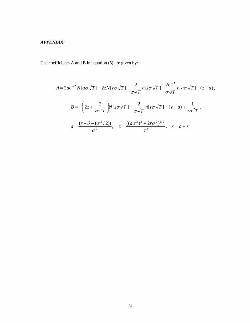
APPENDIX:
The coefficients A and B in equation (5) are given by:
)(][2][2][2][2 azTanT
eTznT
TzzNTaNaeArT
rT −++−−=−
− σσ
σσ
σσ ,
TzazTzn
TTzN
TzzB 22
1)(][2][22σ
σσ
σσ
+−+−⎟⎠⎞
⎜⎝⎛ +−= ,
zaxrazra +=+
=−−
= ,)2)((,))2/((2
2/1222
2
2
σσσ
σσδ