Probabilistic recognition of human faces from video · Probabilistic recognition of human faces from video q Shaohua Zhou,* Volker Krueger, and Rama Chellappa Center for Automation

Computer Vision and Image Understanding 91 (2003) 214–245

www.elsevier.com/locate/cviu

Probabilistic recognition of human facesfrom video q

Shaohua Zhou,* Volker Krueger, and Rama Chellappa

Center for Automation Research (CfAR), Department of Electrical and Computer Engineering,

University of Maryland, College Park, MD 20742, USA

Received 15 February 2002; accepted 11 February 2003

Abstract

Recognition of human faces using a gallery of still or video images and a probe set of videos

is systematically investigated using a probabilistic framework. In still-to-video recognition,

where the gallery consists of still images, a time series state space model is proposed to fuse

temporal information in a probe video, which simultaneously characterizes the kinematics

and identity using a motion vector and an identity variable, respectively. The joint posterior dis-

tribution of the motion vector and the identity variable is estimated at each time instant and

then propagated to the next time instant. Marginalization over the motion vector yields a ro-

bust estimate of the posterior distribution of the identity variable. A computationally efficient

sequential importance sampling (SIS) algorithm is developed to estimate the posterior distribu-

tion. Empirical results demonstrate that, due to the propagation of the identity variable over

time, a degeneracy in posterior probability of the identity variable is achieved to give improved

recognition. The gallery is generalized to videos in order to realize video-to-video recognition.

An exemplar-based learning strategy is adopted to automatically select video representatives

from the gallery, serving as mixture centers in an updated likelihood measure. The SIS algo-

rithm is applied to approximate the posterior distribution of the motion vector, the identity

variable, and the exemplar index, whose marginal distribution of the identity variable pro-

duces the recognition result. The model formulation is very general and it allows a variety

of image representations and transformations. Experimental results using images/videos

collected at UMD, NIST/USF, and CMU with pose/illumination variations illustrate the

qThis work was completed with the support of the DARPA HumanID Grant N00014-00-1-0908. All

correspondences are addressed to [email protected]. Tel: 301-405-4526. Fax: 301-314-9115. Krueger

was affiliated with CfAR. He is now at the Aalborg University, Denmark.* Corresponding author.

E-mail addresses: [email protected] (S. Zhou), [email protected] (V. Krueger), rama@cfar.

umd.edu (R. Chellappa).

1077-3142/$ - see front matter � 2003 Elsevier Inc. All rights reserved.

doi:10.1016/S1077-3142(03)00080-8

mail to: [email protected]

S. Zhou et al. / Computer Vision and Image Understanding 91 (2003) 214–245 215

effectiveness of this approach for both still-to-video and video-to-video scenarios with appro-

priate model choices.

� 2003 Elsevier Inc. All rights reserved.

Keywords: Face recognition; Still-to-video; Video-to-video; Time series state space model; Sequential

importance sampling; Exemplar-based learning

1. Introduction

Probabilistic video analysis has recently gained significant attention in the com-

puter vision community since the seminal work of Isard and Blake [1]. In their effort

to solve the problem of visual tracking, they introduced a time series state spacemodel parameterized by a tracking motion vector (e.g., affine transformation param-

eters), denoted by ht. The CONDENSATION algorithm was developed to provide a

numerical approximation to the posterior distribution of the motion vector at time tgiven the observations up to t, i.e., pðhtjz0:tÞ where z0:t ¼ ðz0; z1; . . . ; ztÞ and zt is theobservation at time t, and to propagate it over time according to the kinematics.

The CONDENSATION algorithm, also known as the particle filter (PF), was orig-

inally proposed in [2] in the signal processing literature and has been used to solve

many other vision tasks [3,4], including human face recognition (FR) [5]. In this pa-per, we will systematically investigate the incorporation of temporal information in a

video sequence for face recognition.

Face recognition has been an extensive research area for a long time. Refer to [6,7]

for surveys and [8] for reports on experiments. Experiments reported in [8] evaluate

still-to-still scenarios, where the gallery and the probe set consist of still facial images.

Some well-known still-to-still FR approaches include Principal Component Analysis

(PCA) [9], Linear Discriminant Analysis (LDA) [10,11], and Elastic Graph Matching

(EGM)[12]. Typically, recognition is performed based on an abstract representationof the face image after suitable geometric and photometric transformations and

corrections.

Following [8], we define a still-to-video scenario: the gallery consists of still facial

templates and the probe set consists of video sequences containing the facial region.

Denote the gallery as I ¼ fI1; I2; . . . ; INg, indexed by the identity variable n, which lies

in a finite sample space N ¼ f1; 2; . . . ;Ng. Though significant research has been con-

ducted on still-to-still recognition, research efforts on still-to-video recognition, are rel-

atively fewer due to the following challenges [7] in typical surveillance applications:poor video quality, significant illumination and pose variations, and low image resolu-

tion.Most existing video-based recognition systems [13] attempt the following: the face

is first detected and then trackedover time.Onlywhen a frame satisfying certain criteria

(size and pose) is acquired, recognition is performed using still-to-still recognition tech-

nique. For this, the face part is cropped from the frame and transformed or registered

using appropriate transformations. This tracking-then-recognition approach attempts

to resolve uncertainties in tracking and recognition sequentially and separately.

216 S. Zhou et al. / Computer Vision and Image Understanding 91 (2003) 214–245

There are several unresolved issues in the tracking-then-recognition approach:

criteria for selecting good frames and estimation of parameters for registra-

tion. Also, still-to-still recognition does not effectively exploit temporal informa-

tion. A common strategy that selects several good frames, performs recognition

on each frame and then votes on these recognition results for a final solutionmight be ad hoc.

To overcome these difficulties, we propose a tracking-and-recognition approach,

which attempts to resolve uncertainties in tracking and recognition simultaneously

in a unified probabilistic framework. To fuse temporal information, the time series

state space model is adopted to characterize the evolving kinematics and identity

in the probe video. Three basic components of the model are:

• a motion equation governing the kinematic behavior of the tracking motion

vector,• an identity equation governing the temporal evolution of the identity variable,

• an observation equation establishing a link between the motion vector and the iden-

tity variable.

Using the sequential importance sampling (SIS) [1,14–16] technique, the joint pos-

terior distribution of the motion vector and the identity variable, i.e., pðnt; htjz0:tÞ isestimated at each time instant and then propagated to the next time instant governed

by motion and identity equations. The marginal distribution of the identity variable,

i.e., pðntjz0:tÞ, is estimated to provide a recognition result. An SIS algorithm is devel-oped to approximate the distribution pðntjz0:tÞ in the still-to-video scenario. It

achieves computational efficiency over its CONDENSATION counterpart by con-

sidering the discrete nature of the identity variable.

The still templates in the gallery can be generalized to video sequences in order to

realize video-to-video recognition. In video-to-video recognition, exemplars and their

prior probabilities are learned from the gallery videos to serve as still templates in the

still-to-video scenario. A person n may have a collection of several exemplars, say

Cn ¼ fcn1; cn2; . . . ; cnKng indexed by k. The likelihood is modified as a mixture density

with exemplars as mixture centers. We first compute the joint distribution

pðnt; kt; htjz0:tÞ using the SIS algorithm and marginalize it to yield pðntjz0:tÞ. In the

experiments reported, the subject walks on a tread-mill with his/her face moving

naturally, giving rise to significant variations across poses. However, the proposed

method successfully cope with these pose variations as evidenced by the experimental

results.

It is worth emphasizing that (i) our model can take advantage of any still-to-still

recognition algorithm [9–12] by embedding distance measures used therein in ourlikelihood measurement and (ii) it allows a variety of image representations and

transformations.

The organization of the paper is as follows: Section 2 reviews some related studies

on (i) face modeling and recognition and (ii) video-based tracking and recognition in

the literature. Section 3 introduces the time series state space model for recognition

and establishes the time-evolving behavior of pðntjz0:tÞ. Section 4 briefly reviews the

SIS principles from the viewpoint of a general state space model and develops a SIS

algorithm to solve the still-to-video recognition problem, with a special emphasis on


its computational efficiency. Section 5 describes the experimental scenarios for still-

to-video recognition and presents results using data collected at UMD, NIST/USF,

and CMU (MoBo database) as part of the HumanID effort. In Section 6, the exem-

plar-based learning algorithm and the SIS algorithm to accommodate video-to-video

recognition are presented. Experimental results for video-to-video recognition prob-lem using the CMU data are also included in this section. Section 7 concludes the

paper with discussions.

2. Related literature

2.1. Face modeling and recognition

Statistical approaches to face modeling have been very popular since Turk and

Pentland�s work on eigenface in 1991 [9]. In statistical approach, the two-dimen-

sional appearance of face image is treated as a vector by scanning the image in

lexicographical order, with the vector dimension being the number of pixels in the

image. In the eigenface approach [9], all face images consists of a distinctive face

subspace. This subspace is linear and spanned by the eigenvectors of the covari-

ance matrix found using PCA. Typically we keep the number of eigenvectors

much less than the true dimension of the vector space. The task of face recogni-tion is then to find the closest match in this face subspace. However, PCA might

not be efficient in terms of recognition accuracy since the construction of the face

subspace does not capture discrimination between humans. This motivates the use

of LDA [11,10] and its variants. In LDA, the linear subspace is constructed [17]

in such a manner that the within-class scatter is minimized and the between-class

scatter is maximized. This idea is further generalized in the approach called

Bayesian face recognition [18], where intra-personal space (IPS) and extra-per-

sonal space (EPS) are used in lieu of within-class scatter and between-class scattermeasures. The IPS models the variations in the appearance of the same individual

and the EPS models the variations in the appearance due to a difference in the

identity. Probabilistic subspace density is then fitted on each space. A Bayesian

decision is taken using a maximum a posteriori (MAP) rule to determine the

identity.

Neural-networks have also been commonly used for face recognition. In the fa-

mous EGM [12] algorithm, the face is represented as a labeled graph, where each

node is labeled with jets derived from responses obtained by convolving the imagewith a family of Gabor functions. The edge characterizes the geometric distance

between two nodes. Face recognition is then formalized as a graph matching

problem.

All the above approaches are based on 2D appearance and perform poorly when

significant pose and illumination variations are present [8]. To completely resolve

such challenges, 3D face modeling [19] is necessary. However, building a 3D face

model is a very difficult and complicated task in the literature even though structure

from motion has been studied for several decades.


2.2. Video-based tracking and recognition

Nearly all video-based recognition systems apply still-image-based recognition to

selected good frames. The face images are warped into frontal views whenever pose

and depth information about the faces is available [13].In [20–22], Radial Basis Function (RBF) networks are used for tracking and recog-

nition purposes. In [20], the system uses an RBF network for recognition. Since no

warping is done, the RBF network has to learn the individual variations as well as pos-

sible transformations. The performance appears to vary widely, depending on the size

of the training data. [22] presents a fully automatic person authentication system. The

system uses video break, face detection, and authentication modules and cycles over

successive video images until a high recognition confidence is reached. This system

was tested on three image sequences; the first was taken indoors with one subject pres-ent, the secondwas taken outdoorswith two subjects, and the thirdwas taken outdoors

with one subject in stormy conditions. Perfect results were reported on all three

sequences, when verified against a database of 20 still face images.

In [23], a system called PersonSpotter is described. This system is able to capture,

track and recognize a person walking toward or passing a stereo CCD camera. It has

several modules, including a head tracker, and a landmark finder. The landmark fin-

der uses a dense graph consisting of 48 nodes learned from 25 example images to find

landmarks such as eyes and nose tip. An elastic graph matching scheme is employedto identify the face.

A multimodal based person recognition system is described in [13]. This system

consists of a face recognition module, a speaker identification module, and a classi-

fier fusion module. The most reliable video frames and audio clips are selected for

recognition. 3D information about the head is used to detect the presence of an ac-

tual person as opposed to an image of that person. Recognition and verification rates

of 100% were achieved for 26 registered clients.

In [24], recognition of face over time is implemented by constructing a face iden-tity surface. The face is first warped to a frontal view, and its Kernel Discriminant

Analysis (KDA) features over time form a trajectory. It is shown that the trajectory

distances accumulate recognition evidence over time.

In [5], a generic approach to simultaneous object tracking and verification is pro-

posed. The approach is based on posterior probability density estimation using se-

quential Monte Carlo methods [1,14–16]. Tracking is formulated as a probability

density propagation problem and the algorithm also provides verification results.

However, no systematic evaluation of recognition was done. Our approach lookssimilar to this algorithm; however, there are significant differences from the algo-

rithm described in [5]. We highlight the differences in Section 7.

3. A model for recognition in video

In this section, we present the details on the propagation model for recognition

and discuss its impact on the posterior distribution of identity variable.


3.1. A time series state space model for recognition

3.1.1. Motion equation

In its most general form, the motion model can be written as

ht ¼ gðht�1; utÞ; tP 1; ð1Þ
where ut is noise in the motion model, whose distribution determines the motion state
transition probability pðhtjht�1Þ. The function gð�; �Þ characterizes the evolving motion

and it could be a function learned offline or given a priori. One of the simplest choice is

an additive function, i.e., ht ¼ ht�1 þ ut, which leads to a first-order Markov chain.

Choice of ht is application dependent. Affine motion parameters are often used

when there is no significant pose variation available in the video sequence. However,if a 3D face model is used, 3D motion parameters should be used accordingly.

3.1.2. Identity equation

nt ¼ nt�1; tP 1; ð2Þ
assuming that the identity does not change as time proceeds.
3.1.3. Observation equation

By assuming that the transformed observation is a noise-corrupted version of

some still template in the gallery, the observation equation can be written as

T htfztg ¼ Int þ vt; tP 1; ð3Þ
where vt is observation noise at time t, whose distribution determines the observation
likelihood pðztjnt; htÞ, and T htfztg is a transformed version of the observation zt. Thistransformation could be either geometric or photometric or both. However, when

confronting sophisticated scenarios, this model is far from sufficient. One should

seek for complicated likelihood measurement as shown in Section 5.

We assume statistical independence between all noise variables and prior knowl-edge on the distributions pðh0jz0Þ and pðn0jz0Þ. Using the overall state vector

xt ¼ ðnt; htÞ, Eqs. (1) and (2) can be combined into one state equation (in a normal

sense) which is completely described by the overall state transition probability

pðxtjxt�1Þ ¼ pðntjnt�1Þpðhtjht�1Þ: ð4Þ

Given this model, our goal is to compute the posterior probability pðntjz0:tÞ. It is infact a probability mass function (PMF) since nt only takes values from

N ¼ f1; 2; . . . ;Ng, as well as a marginal probability of pðnt; htjz0:tÞ, which is a mixed

distribution. Therefore, the problem is reduced to computing the posterior probability.

3.2. The posterior probability of identity variable

The evolution of the posterior probability pðntjz0:tÞ as time proceeds is very inter-

esting to study as the identity variable does not change by assumption, i.e.,pðntjnt�1Þ ¼ dðnt � nt�1Þ, where dð�Þ is a discrete impulse function at zero.


Using time recursion, Markov properties, and statistical independence embedded

in the model, we can easily derive:

pðn0:t; h0:tjz0:tÞ ¼ pðn0:t�1; h0:t�1jz0:t�1Þpðztjnt; htÞpðntjnt�1Þpðhtjht�1Þ

pðztjz0:t�1Þ

¼ pðn0; h0jz0ÞYt

s¼1

pðzsjns; hsÞpðnsjns�1Þpðhsjhs�1Þpðzsjz0:s�1Þ

¼ pðn0jz0Þpðh0jz0ÞYt

s¼1

pðzsjns; hsÞdðns � ns�1Þpðhsjhs�1Þpðzsjz0:s�1Þ

: ð5Þ

Therefore, by marginalizing over h0:t and n0:t�1, we obtain

pðnt ¼ ljz0:tÞ ¼ pðljz0ÞZh0

� � �Zht

pðh0jz0ÞYt

s¼1

pðzsjl; hsÞpðhsjhs�1Þpðzsjz0:s�1Þ

dht � � � dh0: ð6Þ

Thus pðnt ¼ ljz0:tÞ is determined by the prior distribution pðn0 ¼ ljz0Þ and the

product of the likelihood functions,Qt

s¼1 pðzsjl; hsÞ. If a uniform prior is assumed,

thenQt

s¼1 pðzsjl; hsÞ is the only determining factor.In the Appendix A, we show that, under some minor assumptions, the posterior

probability for the correct identity l, pðnt ¼ ljz0:tÞ, is lower-bounded by an increasing

curve which converges to 1.

To measure the evolving uncertainty remaining in the identity variable as obser-

vations accumulate, we use the notion of entropy [25]. In the context of this problem,

conditional entropy Hðntjz0:tÞ is used. However, the knowledge of pðz0:tÞ is needed to

compute Hðntjz0:tÞ. We assume that it degenerates to an impulse at the actual obser-

vations ~zz0:t since we observe only this particular sequence, i.e., pðz0:tÞ ¼ dðz0:t � ~zz0:tÞ.Now,

Hðntjz0:tÞ ¼ �Xnt2N

pðntj~zz0:tÞ log2 pðntj~zz0:tÞ: ð7Þ

Under the assumptions listed in the Appendix A, we expect that Hðntjz0:tÞdecreases as time proceeds since we start from an equi-probable distribution to a

degenerate one.

4. Sequential importance sampling algorithm

Consider a general time series state space model fully determined by (i) the overallstate transition probability pðxtjxt�1Þ, (ii) the observation likelihood pðztjxtÞ, and (iii)

prior probability pðx0jz0Þ and statistical independence among all noise variables. We

wish to compute the posterior probability pðxtjz0:tÞ.If the model is linear with Gaussian noise, it is analytically solvable by a Kalman

filter which essentially propagates the mean and variance of a Gaussian distribution

over time. For non-linear and non-Gaussian cases, an extended Kalman filter (EKF)

and its variants have been used to arrive at an approximate analytic solution [26].


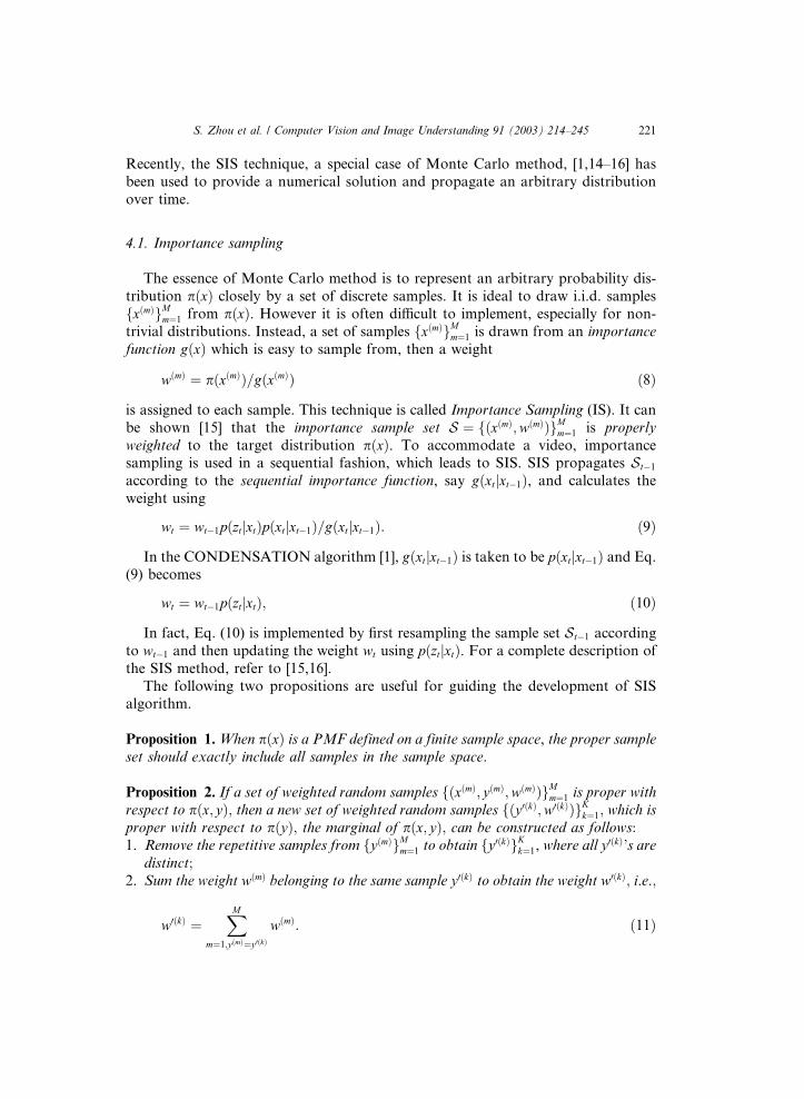
Recently, the SIS technique, a special case of Monte Carlo method, [1,14–16] has

been used to provide a numerical solution and propagate an arbitrary distribution

over time.

4.1. Importance sampling

The essence of Monte Carlo method is to represent an arbitrary probability dis-

tribution pðxÞ closely by a set of discrete samples. It is ideal to draw i.i.d. samples

fxðmÞgMm¼1 from pðxÞ. However it is often difficult to implement, especially for non-

trivial distributions. Instead, a set of samples fxðmÞgMm¼1 is drawn from an importance

function gðxÞ which is easy to sample from, then a weight

wðmÞ ¼ pðxðmÞÞ=gðxðmÞÞ ð8Þ

is assigned to each sample. This technique is called Importance Sampling (IS). It can

be shown [15] that the importance sample set S ¼ fðxðmÞ;wðmÞÞgMm¼1 is properly

weighted to the target distribution pðxÞ. To accommodate a video, importancesampling is used in a sequential fashion, which leads to SIS. SIS propagates St�1according to the sequential importance function, say gðxtjxt�1Þ, and calculates the

weight using

wt ¼ wt�1pðztjxtÞpðxtjxt�1Þ=gðxtjxt�1Þ: ð9Þ

In the CONDENSATION algorithm [1], gðxtjxt�1Þ is taken to be pðxtjxt�1Þ and Eq.(9) becomes

wt ¼ wt�1pðztjxtÞ; ð10Þ

In fact, Eq. (10) is implemented by first resampling the sample set St�1 accordingto wt�1 and then updating the weight wt using pðztjxtÞ. For a complete description of

the SIS method, refer to [15,16].

The following two propositions are useful for guiding the development of SISalgorithm.

Proposition 1.When pðxÞ is a PMF defined on a finite sample space, the proper sampleset should exactly include all samples in the sample space.

Proposition 2. If a set of weighted random samples fðxðmÞ; yðmÞ;wðmÞÞgMm¼1 is proper withrespect to pðx; yÞ; then a new set of weighted random samples fðy0ðkÞ;w0ðkÞÞgKk¼1; which isproper with respect to pðyÞ; the marginal of pðx; yÞ; can be constructed as follows:1. Remove the repetitive samples from fyðmÞgMm¼1 to obtain fy0ðkÞg

Kk¼1, where all y

0ðkÞ’s aredistinct;

2. Sum the weight wðmÞ belonging to the same sample y0ðkÞ to obtain the weight w0ðkÞ; i.e.;

w0ðkÞ ¼XM

m¼1;yðmÞ¼y0ðkÞwðmÞ: ð11Þ


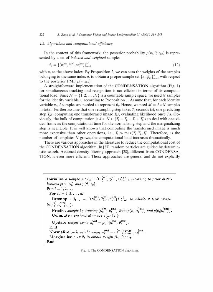
4.2. Algorithms and computational efficiency

In the context of this framework, the posterior probability pðnt; htjz0:tÞ is repre-

sented by a set of indexed and weighted samples

St ¼ fðnðmÞt ; hðmÞt ;wðmÞt ÞgMm¼1 ð12Þ

with nt as the above index. By Proposition 2, we can sum the weights of the samplesbelonging to the same index nt to obtain a proper sample set fnt; bntg

Nnt¼1 with respect

to the posterior PMF pðntjz0:tÞ.A straightforward implementation of the CONDENSATION algorithm (Fig. 1)

for simultaneous tracking and recognition is not efficient in terms of its computa-

tional load. Since N ¼ f1; 2; . . . ;Ng is a countable sample space, we need N samples

for the identity variable nt according to Proposition 1. Assume that, for each identity

variable nt, J samples are needed to represent ht. Hence, we need M ¼ J � N samples

in total. Further assume that one resampling step takes Tr seconds (s), one predictingstep Tps, computing one transformed image Tts, evaluating likelihood once Tls. Ob-

viously, the bulk of computation is J � N � ðTr þ Tp þ Tt þ TlÞs to deal with one vi-

deo frame as the computational time for the normalizing step and the marginalizing

step is negligible. It is well known that computing the transformed image is much

more expensive than other operations, i.e., Tt � maxðTr; Tp; TlÞ. Therefore, as the

number of templates N grows, the computational load increases dramatically.

There are various approaches in the literature to reduce the computational cost of

the CONDENSATION algorithm. In [27], random particles are guided by determin-istic search. Assumed density filtering approach [28], different from CONDENSA-

TION, is even more efficient. Those approaches are general and do not explicitly

Fig. 1. The CONDENSATION algorithm.


exploit the special structure of the distribution in this setting: a mixed distribution

of continuous and discrete variables. To this end, we propose the following

algorithm.

As the sample space N is countable, an exhaustive search of sample space N is

possible. Mathematically, we release the random sampling in the identity variablent by constructing samples as follows: for each hðjÞt ,

ð1; hðjÞt ;wðjÞt;1Þ; ð2; hðjÞt ;wðjÞt;2Þ; . . . ; ðN ; hðjÞt ;wðjÞt;N Þ:

We in fact use the following notation for the sample set,

St ¼ fðhðjÞt ;wðjÞt ;wðjÞt;1 ;wðjÞt;2 ; . . . ;w

ðjÞt;N Þg

Jj¼1; ð13Þ

with wðjÞt ¼PN

n¼1 wðjÞt;n . The proposed algorithm is summarized in Fig. 2.

The crux of this algorithm lies in that, instead of propagating random samples on

both motion vector and identity variable, we can keep the samples on the identityvariable fixed and let those on the motion vector be random. Although we propagate

only the marginal distribution for motion tracking, we still propagate the joint dis-

tribution for recognition purposes.

The bulk of computation of the proposed algorithm is J � ðTr þ Tp þ TtÞþJ � N � Tls, a tremendous improvement over the CONDENSATION when dealing

with a large database since the dominant computational time J � Tt does not dependon N .

Fig. 2. The proposed algorithm.


5. Still-to-video based face recognition

In this section we describe the still-to-video scenarios used in our experiments and

their practical model choices, followed by a discussion of experiments. Three data-

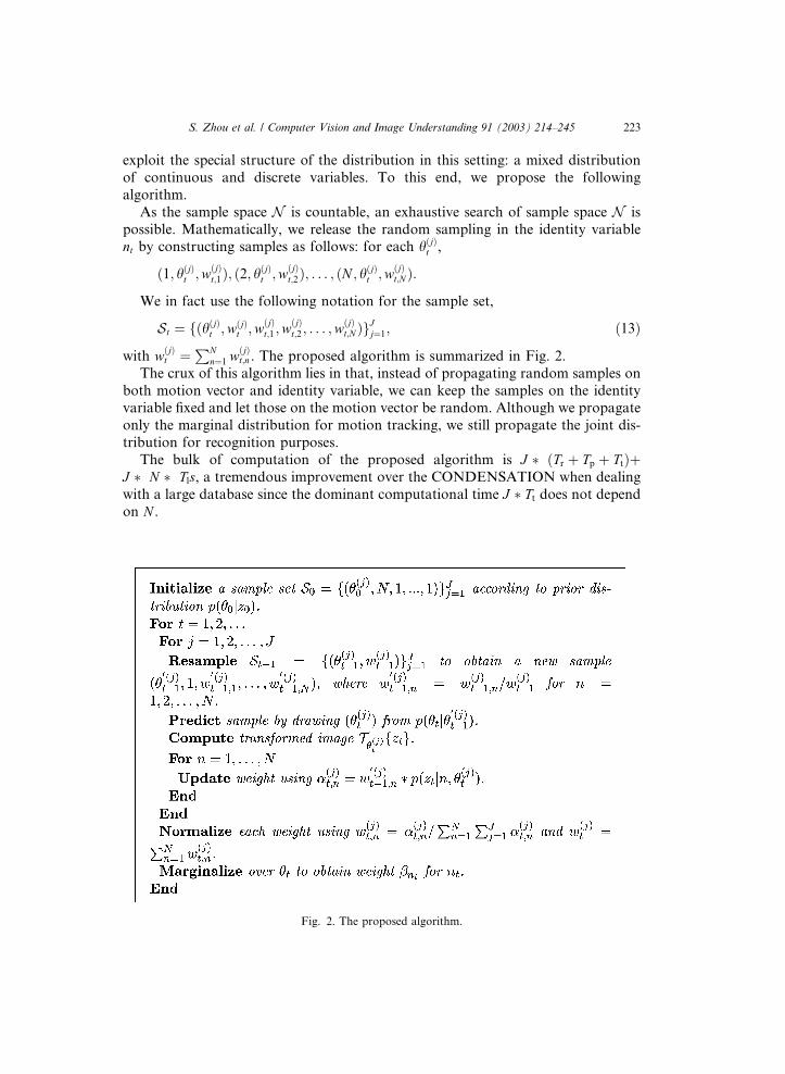
bases are used in the still-to-video experiments.Database-0 was collected outside a building. We mounted a video camera on a

tripod and requested subjects to walk straight towards the camera in order to simu-

late typical scenarios in visual surveillance. Database-0 includes one face gallery, and

one probe set. The images in the gallery are listed in Fig. 3. The probe contains 12

videos, one for each individual. Fig. 3 gives some frames in a probe video.

Fig. 3. Database-0. The 1st row: the face gallery with image size being 30� 26. The 2nd and 3rd rows: 4

example frames in one probe video with image size being 320� 240 while the actual face size ranges ap-

proximately from 30� 30 in the first frame to 50� 50 in the last frame. Notice that the sequence is taken

under a well-controlled condition so that there are no illumination or pose variations between the gallery

and the probe.


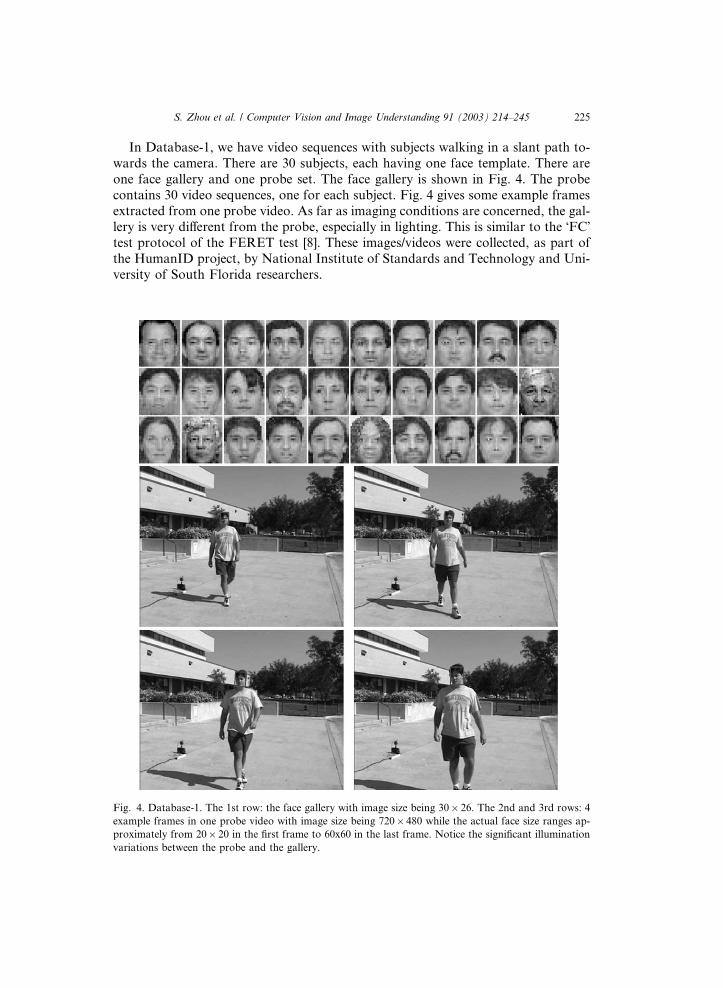
In Database-1, we have video sequences with subjects walking in a slant path to-

wards the camera. There are 30 subjects, each having one face template. There are

one face gallery and one probe set. The face gallery is shown in Fig. 4. The probe

contains 30 video sequences, one for each subject. Fig. 4 gives some example frames

extracted from one probe video. As far as imaging conditions are concerned, the gal-lery is very different from the probe, especially in lighting. This is similar to the �FC�test protocol of the FERET test [8]. These images/videos were collected, as part of

the HumanID project, by National Institute of Standards and Technology and Uni-

versity of South Florida researchers.

Fig. 4. Database-1. The 1st row: the face gallery with image size being 30� 26. The 2nd and 3rd rows: 4

example frames in one probe video with image size being 720� 480 while the actual face size ranges ap-

proximately from 20� 20 in the first frame to 60x60 in the last frame. Notice the significant illumination

variations between the probe and the gallery.


Database-2, Motion of Body (MoBo) database, was collected at the Carnegie

Mellon University [29] under the HumanID project. There are 25 different individu-

als in total. The video sequences show the individuals walking on a tread-mill so that

they move their heads naturally. Different walking styles have been simulated to as-

sure a variety of conditions that are likely to appear in real life: walking slowly, walk-ing fast, inclining, and carrying an object. Therefore, four videos per person and 99

videos in total ( with one carrying video missing ) are available. However, the probe

set we use in this section includes only 25 slowWalk videos. Some example images of

the videos (slowWalk) are shown in Fig. 5. Fig. 5 also shows the face gallery in Da-

tabase-2 with face images in almost frontal view cropped from probe videos and then

normalized using their eye positions.

Table 1 summaries the features of the three databases.

5.1. Results for Database-0

We consider affine transformation. Specifically, the motion is characterized by

h ¼ ða1; a2; a3; a4; tx; tyÞ where fa1; a2; a3; a4g are deformation parameters and ftx; tygare 2D translation parameters. It is a reasonable approximation since there is no sig-

nificant out-of-plane motion as the subjects walk towards the camera. Regarding the

photometric transformation, only zero-mean-unit-variance operator is performed to

partially compensate for contrast variations. The complete transformation T hfzg isprocessed as follows: affine transform z using fa1; a2; a3; a4g, crop out the interested

region at position ftx; tyg with the same size as the still template in the gallery, and

perform zero-mean-unit-variance operation.

Prior distribution pðh0jz0Þ is assumed to be Gaussian, whose mean comes from the

initial detector and whose covariance matrix is manually specified.

A time-invariant first-order Markov Gaussian model with constant velocity is

used for modeling motion transition. Given the scenario that the subject is walking

towards the camera, the scale increases with time. However, under perspective pro-jection, this increase is no longer linear, causing the constant-velocity model to be

not optimal. However, experimental results show that as long as the samples of hcan cover the motion, this model is sufficient.

The likelihood measurement is simply set as a �truncated� Laplacian:

p1ðztjnt; htÞ ¼ LAPðkT htfztg � Intk; r1; s1Þ; ð14Þ
where, k � k is sum of absolute distance, r1 and k1 are manually specified, and
LAPðx; r; sÞ ¼ r�1 expð�x=rÞ if x6 sr;r�1 expð�sÞ otherwise:

�ð15Þ

Gaussian distribution is widely used as a noise model, accounting for sensor noise,

digitization noise, etc. However, given the observation equation: vt ¼ T htfztg � Int ,the dominant part of vt becomes the high-frequency residual if ht is not proper,

and it is well known that the high-frequency residual of natural images is more La-placian-like. The �truncated� Laplacian is used to give a �surviving� chance for sam-

ples to accommodate abrupt motion changes.

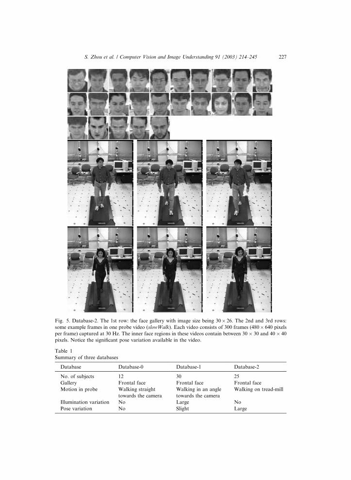
Table 1

Summary of three databases

Database Database-0 Database-1 Database-2

No. of subjects 12 30 25

Gallery Frontal face Frontal face Frontal face

Motion in probe Walking straight

towards the camera

Walking in an angle

towards the camera

Walking on tread-mill

Illumination variation No Large No

Pose variation No Slight Large

Fig. 5. Database-2. The 1st row: the face gallery with image size being 30� 26. The 2nd and 3rd rows:

some example frames in one probe video (slowWalk). Each video consists of 300 frames (480� 640 pixels

per frame) captured at 30 Hz. The inner face regions in these videos contain between 30� 30 and 40� 40

pixels. Notice the significant pose variation available in the video.



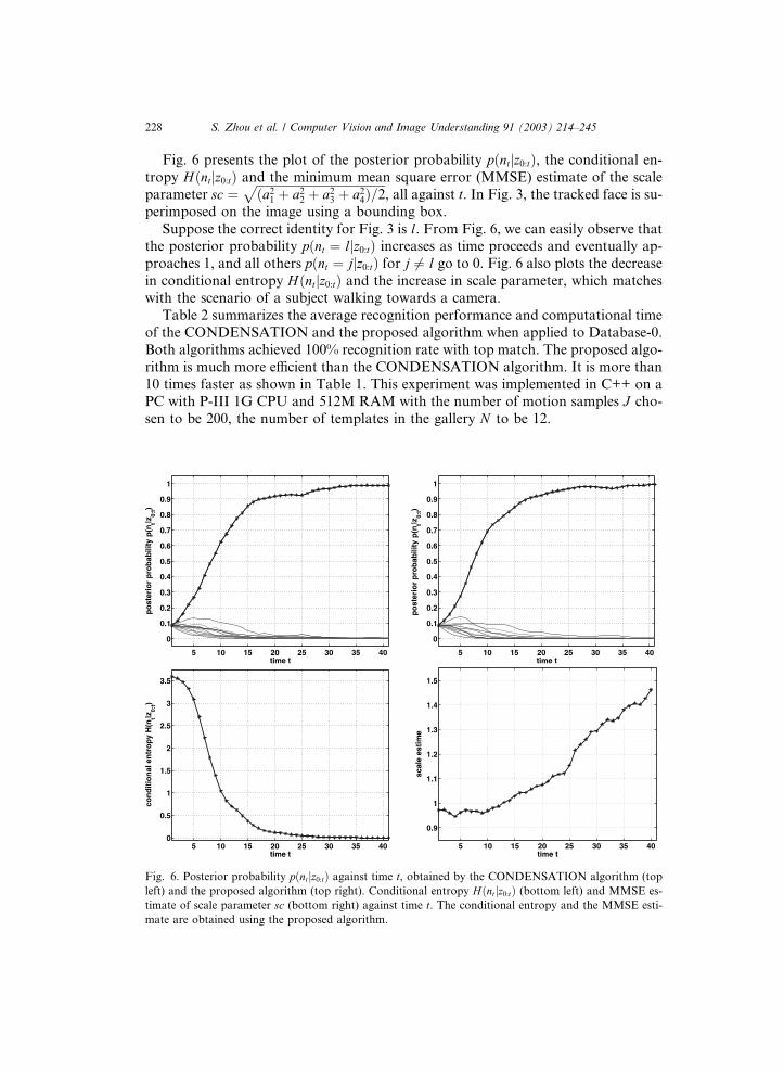
Fig. 6 presents the plot of the posterior probability pðntjz0:tÞ, the conditional en-

tropy Hðntjz0:tÞ and the minimum mean square error (MMSE) estimate of the scale

parameter sc ¼ffiffiffiffiffiffiffiffiffiffiffiffiffiffiffiffiffiffiffiffiffiffiffiffiffiffiffiffiffiffiffiffiffiffiffiffiffiffiffiffiffiffiffiða21 þ a22 þ a23 þ a24Þ=2

p, all against t. In Fig. 3, the tracked face is su-

perimposed on the image using a bounding box.

Suppose the correct identity for Fig. 3 is l. From Fig. 6, we can easily observe thatthe posterior probability pðnt ¼ ljz0:tÞ increases as time proceeds and eventually ap-

proaches 1, and all others pðnt ¼ jjz0:tÞ for j 6¼ l go to 0. Fig. 6 also plots the decrease

in conditional entropy Hðntjz0:tÞ and the increase in scale parameter, which matches

with the scenario of a subject walking towards a camera.

Table 2 summarizes the average recognition performance and computational time

of the CONDENSATION and the proposed algorithm when applied to Database-0.

Both algorithms achieved 100% recognition rate with top match. The proposed algo-

rithm is much more efficient than the CONDENSATION algorithm. It is more than10 times faster as shown in Table 1. This experiment was implemented in C++ on a

PC with P-III 1G CPU and 512M RAM with the number of motion samples J cho-

sen to be 200, the number of templates in the gallery N to be 12.

Fig. 6. Posterior probability pðntjz0:tÞ against time t, obtained by the CONDENSATION algorithm (top

left) and the proposed algorithm (top right). Conditional entropy Hðntjz0:tÞ (bottom left) and MMSE es-

timate of scale parameter sc (bottom right) against time t. The conditional entropy and the MMSE esti-

mate are obtained using the proposed algorithm.

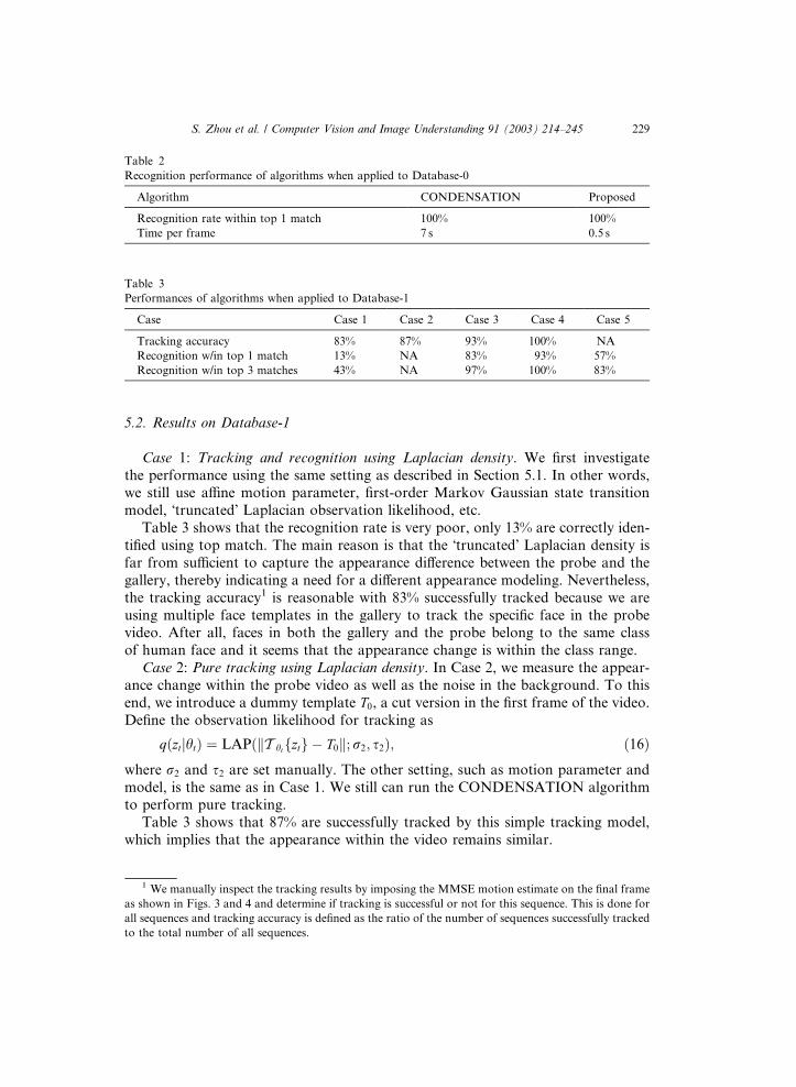
Table 2

Recognition performance of algorithms when applied to Database-0

Algorithm CONDENSATION Proposed

Recognition rate within top 1 match 100% 100%

Time per frame 7 s 0.5 s

Table 3

Performances of algorithms when applied to Database-1

Case Case 1 Case 2 Case 3 Case 4 Case 5

Tracking accuracy 83% 87% 93% 100% NA

Recognition w/in top 1 match 13% NA 83% 93% 57%

Recognition w/in top 3 matches 43% NA 97% 100% 83%


5.2. Results on Database-1

Case 1: Tracking and recognition using Laplacian density. We first investigate

the performance using the same setting as described in Section 5.1. In other words,we still use affine motion parameter, first-order Markov Gaussian state transition

model, �truncated� Laplacian observation likelihood, etc.

Table 3 shows that the recognition rate is very poor, only 13% are correctly iden-

tified using top match. The main reason is that the �truncated� Laplacian density is

far from sufficient to capture the appearance difference between the probe and the

gallery, thereby indicating a need for a different appearance modeling. Nevertheless,

the tracking accuracy1 is reasonable with 83% successfully tracked because we are

using multiple face templates in the gallery to track the specific face in the probevideo. After all, faces in both the gallery and the probe belong to the same class

of human face and it seems that the appearance change is within the class range.

Case 2: Pure tracking using Laplacian density. In Case 2, we measure the appear-

ance change within the probe video as well as the noise in the background. To this

end, we introduce a dummy template T0, a cut version in the first frame of the video.

Define the observation likelihood for tracking as

1 W

as sho

all seq

to the

qðztjhtÞ ¼ LAPðkT htfztg � T0k;r2; s2Þ; ð16Þ
where r2 and s2 are set manually. The other setting, such as motion parameter and
model, is the same as in Case 1. We still can run the CONDENSATION algorithmto perform pure tracking.

Table 3 shows that 87% are successfully tracked by this simple tracking model,

which implies that the appearance within the video remains similar.

e manually inspect the tracking results by imposing the MMSE motion estimate on the final frame

wn in Figs. 3 and 4 and determine if tracking is successful or not for this sequence. This is done for

uences and tracking accuracy is defined as the ratio of the number of sequences successfully tracked

total number of all sequences.


Case 3: Tracking and recognition using probabilistic subspace density. As men-

tioned in Case 1, we need a new appearance model to improve the recognition accu-

racy. As reviewed in Section 2.1, there are various approaches in the literature. We

decided to use the approach suggested by Moghaddam et. al. [18] due to its compu-

tational efficiency and high recognition accuracy. However, in our implementation,we model only intra-personal variations instead of both intra/extra-personal varia-

tions for simplicity.

We need at least two facial images for one identity to construct the intra-personal

space (IPS). Apart from the available gallery, we crop out the second image from the

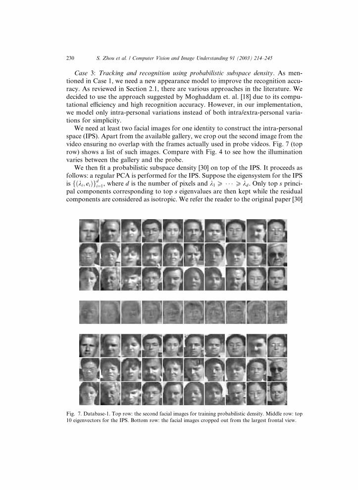
video ensuring no overlap with the frames actually used in probe videos. Fig. 7 (top

row) shows a list of such images. Compare with Fig. 4 to see how the illumination

varies between the gallery and the probe.

We then fit a probabilistic subspace density [30] on top of the IPS. It proceeds asfollows: a regular PCA is performed for the IPS. Suppose the eigensystem for the IPS

is fðki; eiÞgdi¼1, where d is the number of pixels and k1 P � � � P kd . Only top s princi-pal components corresponding to top s eigenvalues are then kept while the residual

components are considered as isotropic. We refer the reader to the original paper [30]

Fig. 7. Database-1. Top row: the second facial images for training probabilistic density. Middle row: top

10 eigenvectors for the IPS. Bottom row: the facial images cropped out from the largest frontal view.


for full details. Fig. 7 (middle row) show the eigenvectors for the IPS. The density is

written as follows:

PSðxÞ ¼exp � ð1=2Þ

Psi¼1ðy2i =kiÞ

� �ð2pÞs=2

Qsi¼1 k

1=2i

( )exp � �2=2qð Þð2pqÞðd�sÞ=2

( ); ð17Þ

where yi ¼ eTi x for i ¼ 1; . . . ; s is the ith principal component of x, �2 ¼ kxk2�Ps

i¼1 y2i

is the reconstruction error, and q ¼ ðPd

i¼sþ1 kiÞ=ðd � qÞ. It is easy to write the like-

lihood as follows:

p2ðztjnt; htÞ ¼ PSðT htfztg � Int Þ: ð18Þ
Table 3 lists the performance by using this new likelihood measurement. It turns
out that the performance is significantly better that in Case 1, with 93% tracked suc-cessfully and 83% recognized within top 1 match. If we consider the top 3 matches,

97% are correctly identified.

Case 4: Tracking and recognition using combined density. In Case 2, we have stud-

ied appearance changes within a video sequence. In Case 3, we have studied the ap-

pearance change between the gallery and the probe. In Case 4, we attempt to take

advantage of both cases by introducing a combined likelihood defined as follows:

p3ðztjnt; htÞ ¼ p2ðztjnt; htÞqðztjhtÞ: ð19Þ
Again, all other setting is the same as in Case 1. We now obtain the best perfor-
mance so far: no tracking error, 93% are correctly recognized as the first match, and

no error in recognition when top 3 matches are considered.

Case 5: Still-to-still face recognition. To make a comparison, we also performed an

experiment on still-to-still face recognition. We selected the probe video frames with

the best frontal face view (i.e., biggest frontal view) and cropped out the facial regionby normalizing with respect to the eye coordinates manually specified. This collec-

tion of images is shown in Fig. 7 (bottom row) and it is fed as probes into a still-

to-still face recognition system with the learned probabilistic subspace as in

Case 3. It turns out that the recognition result is 57% correct for the top one match,

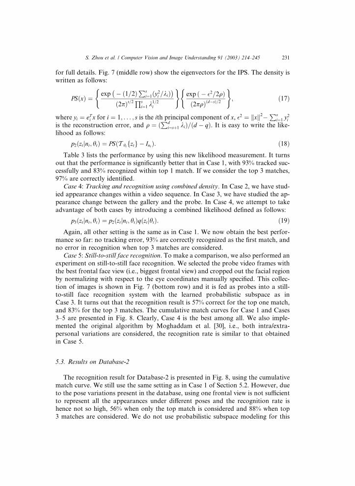
and 83% for the top 3 matches. The cumulative match curves for Case 1 and Cases

3–5 are presented in Fig. 8. Clearly, Case 4 is the best among all. We also imple-

mented the original algorithm by Moghaddam et al. [30], i.e., both intra/extra-

personal variations are considered, the recognition rate is similar to that obtainedin Case 5.

5.3. Results on Database-2

The recognition result for Database-2 is presented in Fig. 8, using the cumulative

match curve. We still use the same setting as in Case 1 of Section 5.2. However, due

to the pose variations present in the database, using one frontal view is not sufficient

to represent all the appearances under different poses and the recognition rate ishence not so high, 56% when only the top match is considered and 88% when top

3 matches are considered. We do not use probabilistic subspace modeling for this

Fig. 8. Cumulative match curves for Database-1 (left) and Database-2 (right).


database because such modeling requires manually cropping out multiple templates

for each individual. Also, pre-selecting video frames from the same probe video and

ensuring that they do not overlap with the probe frames is time-consuming. What is

desirable is to automatically select such templates from different sources other than

the probe video. Since we have multiple videos available for one individual in Data-

base-2, this motivates us to obtain more representative views for one face class, lead-ing to the discussions in the next section.

6. Video-to-video based face recognition

In this section we introduce a video-to-video based face recognition approach. It

enhances the still-to-video approach by taking an entire video, instead of a single im-

age, to represent the face of an individual. The video-to-video based approach hastwo stages: In the learning stage, Exemplars, which are selected representatives from

the raw video, are automatically extracted from gallery videos. The exemplars are

used to summarize the gallery video information. In the recognition stage, exemplars

are then used as centers for probabilistic mixture distributions for tracking and rec-

ognition processes. Probabilistic methods are attractive in this context as they allow

a systematic handling of uncertainty and an elegant way for fusing temporal infor-

mation.

In Section 6.1 we present the learning stage and explain, how the exemplars aregenerated from a gallery video. In Section 6.2 we explain how tracking and recogni-

tion steps are implemented. In Section 6.3 we present experimental results on 99

video sequences of 25 individuals in Database-2.

6.1. Exemplar-based learning

In order to realize video-to-video recognition, a probabilistic model needs to

be learned from each gallery video V . Denote the gallery as V ¼ fV1; V2; . . . ; VNg.


For this, we take an approach which is similar to the ones proposed in [31,32]. These

two approaches try to find a set of exemplars that describe the set of training images

best, i.e., that minimize the expected distance between the given set of images

Z ¼ fz1; z2; . . . ; zJg and a set of exemplars (cluster centers) C ¼ fc1; c2; . . . ; cKg.In other words, let Z ¼ fz1; z2; . . . ; zJg again be the sequence of video images. It is

being searched for a set of exemplars C ¼ fc1; c2; . . . ; cKg such that

pðztÞ ¼Xc2C

ZHpðztjh; cÞpðhjcÞpðcÞdh ð20Þ

is maximal for all t. Here, pðztjh; cÞ is the observation equation, given as

pðztjxÞ � pðztjh; cÞ / exp

�� 1

2r2dðT hfztg; cÞ

�; ð21Þ

where the choice of r depends on the choice of d, with d being a distance measure.

In [31], the K-means clustering technique is applied to minimize Eq. (20), and in

[32] the EM approach is used. The application of the EM approach has drawbacks

that were already pointed out by [31]. The application of a K-means clustering tech-

nique, as proposed in [31] has, however, the following drawbacks:

• K has to be given in advance. For face recognition this drawback is restrictive:Clearly, the distance measure d may be chosen arbitrarily and for face recognition

it is preferable to choose one of the well known ones (e.g., PCA, bunch graph) [8].

Thresholds and variances for each of these measures that minimize mis-classifica-

tion are known and considering them requires a dynamic choice of the number of

clusters rather than a static one.

• Storing the training data in order to compute the clusters becomes computation-

ally intensive for long video streams.

We therefore propose an online technique to learn the exemplars which was in-spired by the probabilistic interpretation of the RBF neural network [33]: At each

time step t, pðztjh; cÞ of Eq. (20) is maximized. If pðztjh; cÞ < q for some q (which

depends on the choice of d) then T hfztg is added to the set of exemplars.

The details of the learning algorithm are as follows.

1. The first step is the alignment or tracking: a cluster k and a deformation h 2 H is

found such that dðT hfztg; ckÞ is minimized:

ht arg minh

mink

dðT hfztg; ckÞ and kt argminkdðT htfztg; ckÞ: ð22Þ

2. The second step generates a new cluster center, if necessary: if

pðztjht; cktÞ < q

then

C C [ fT htfztgg:
Count the number of times, countðktÞ ¼ countðktÞ þ 1, that cluster ckt approximates
image zt best.3. Repeat steps one and two until all the frames in the video are processed.


4. Compute the mixture weights lk / countðkÞ.The result of this learning procedure is

1. A set C ¼ fc1; c2; . . . ; cKg of aligned exemplars ck.2. A prior lk for each of the exemplars ck.

Clearly, the more careful the set H is chosen, the fewer exemplars are generated.Allowing H, e.g., to compensate only for translations, exemplars are generated to

compensate scale changes and rotation.

Given a gallery V of videos, the above has to be carried out for each video. During

recognition, as will be explained in the next section, the exemplars are used as centers

of mixture models.

The above learning algorithm is motivated by the online learning approaches for

artificial neural networks (ANNs) [34,35] and clearly, many enhancements can be at-

tempted (topology preserving maps, neighborhood relations, etc.). An online learn-ing algorithm for exemplars used during testing could allow, in a bootstrapping

manner, to learn new exemplars from probe videos.

In [22] a similar learning approach was presented. Contrary to our work, face im-

ages are not normalized with respect to H which results in a far larger number of

clusters. In [20] a �Unit Face� RBF model is proposed where for each individual, a

single RBF network is trained. The authors have also investigated different geomet-

rical normalizations and have experimented with a preprocessing step, such as the

application of a �difference of Gaussians� or Gabor wavelets.The goal of both of these works was to build a representation of a face intensity

by using an RBF network. We want to make clear, that this is exactly what we do

not want! Our intention is, to chose a well-known face representation in advance(such as, e.g., PCA). Then, we learn the different exemplars of a single face. The ad-

vantage is that this way we inherit the ‘‘face recognition capabilities’’ of PCA, LDA

techniques.

6.2. Tracking and recognition with multiple exemplars

After the application of the learning algorithm we have for each individual n a set

of exemplars Cn ¼ fcn1; cn2; . . . ; cnKng. In order to recognize individuals with multiple

exemplars, the SIS-approach has to be developed further.

6.2.1. Exemplars as mixture centers

To take into account a set of exemplars Cn ¼ fcn1; cn2; . . . ; cnKng for individual n, we

refine the likelihood computation of Eq. (21) as follows:

pðztjxÞ � pðztjn; hÞ/

Xc2Cn

pðztjh; cÞpnðcÞ ð23Þ

/X

exp

�� 1

2r2dðT hfzg; cÞ

�lnc : ð24Þ

c2Cn


The exemplars in Cnt are used as the mixture center of a joint distribution and

pntðcÞ ¼ lntc is the prior for mixture center c of individual nt.

6.2.2. Dynamic model

In Section 5, a dynamic model for Eq. (1) has to be given in advance. However,while learning exemplars from video sequences, a dynamic model can also be

learned. In Eq. (4)

pðxtjxt�1Þ � pðht; ntjht�1; nt�1Þ
defines the probability of the state variable to change from xt�1 to xt. Discussions on
learning the dynamic model may be founded in [36,31].

6.2.3. Computation of posterior distribution

The posterior probability distribution pðnt; kt; htjz0:tÞ (where n refers to the individ-

ual and k to the exemplar index) is represented by a set of M indexed and weighted

particles

nðmÞ; kðmÞ; hðmÞ;wðmÞ� �n ot

m¼1;...;M: ð25Þ

Note that we have, for better readability, indexed the entire set with t, instead of each

component. Since all exemplars per person are aligned, we do not have to treat the

different exemplars for a single person separately. We can therefore increase effi-

ciency if we rewrite (25) as:

nðmÞ; 1; hðmÞ;wðmÞ1

..

.

nðmÞ;KnðmÞ ; hðmÞ;wðmÞK

nðmÞ

2664

3775

8>><>>:

9>>=>>;

t

m¼1;...;M 0

: ð26Þ

Set (26) is a set of KnðmÞ � 4 dimensional matrices, and each matrix represents one

particle, where KnðmÞ ¼ jCnðmÞ j. We can now easily marginalize over CnðmÞ to compute

the posterior probability pðnt; htjz0:tÞ: We get with

wwðmÞ ¼XKnðmÞ

k¼1lnðmÞ

k wðmÞk ð27Þ

a new set of weighted sample vectors:

nðmÞ; hðmÞ; wwðmÞ� �n ot

m¼1;...;M 0: ð28Þ

In Eq. (27), lnðmÞk is the prior of exemplar k of person nðmÞ.

To compute the identity from the particle set (28) we marginalize over h as in Eq.

(11).

6.3. Experimental results

We have tested the video-to-video based recognition algorithm on 99 video se-

quences of 25 different individuals in Database-2. As mentioned before, there are


four walking styles: walking slowly, walking fast, inclining, and carrying an object.Therefore, four videos per person are available. In the experiments we used one or

two of the video types as gallery videos for training while the remaining ones were

used as probes for testing.

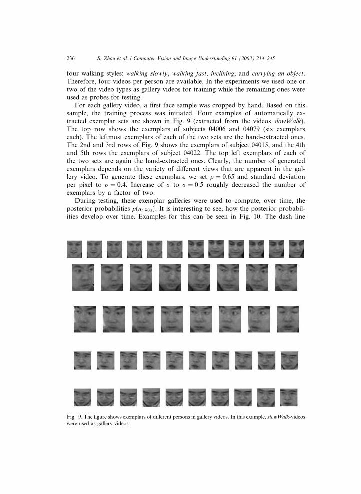
For each gallery video, a first face sample was cropped by hand. Based on thissample, the training process was initiated. Four examples of automatically ex-

tracted exemplar sets are shown in Fig. 9 (extracted from the videos slowWalk).The top row shows the exemplars of subjects 04006 and 04079 (six exemplars

each). The leftmost exemplars of each of the two sets are the hand-extracted ones.

The 2nd and 3rd rows of Fig. 9 shows the exemplars of subject 04015, and the 4th

and 5th rows the exemplars of subject 04022. The top left exemplars of each of

the two sets are again the hand-extracted ones. Clearly, the number of generated

exemplars depends on the variety of different views that are apparent in the gal-lery video. To generate these exemplars, we set q ¼ 0:65 and standard deviation

per pixel to r ¼ 0:4. Increase of r to r ¼ 0:5 roughly decreased the number of

exemplars by a factor of two.

During testing, these exemplar galleries were used to compute, over time, the

posterior probabilities pðntjz0:tÞ. It is interesting to see, how the posterior probabil-

ities develop over time. Examples for this can be seen in Fig. 10. The dash line

Fig. 9. The figure shows exemplars of different persons in gallery videos. In this example, slowWalk-videos

were used as gallery videos.

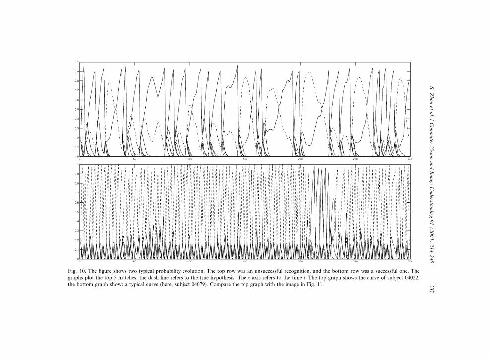
Fig. 10. The figure shows two typical probability evolution. The top row was an unsuccessful recognition, and the bottom row was a successful one. The

graphs plot the top 5 matches, the dash line refers to the true hypothesis. The x-axis refers to the time t. The top graph shows the curve of subject 04022,

the bottom graph shows a typical curve (here, subject 04079). Compare the top graph with the image in Fig. 11.

S.Zhouet

al./Computer

Visio

nandIm

ageUndersta

nding91(2003)214–245

237


refers to the correct hypothesized identity, the other five curves refer to the prob-

abilities of the top matching identities other than the true one. One can see in

the left and the right plots that the dash line (true hypothesis) increases quickly

to one. In order to consider all the frames of the video, we restart the algorithm

after convergence. Recognition is established by that identity, to which the SIS con-verges most often.

Examples illustrating the robustness as well as of the limits of our approach are

shown in Figs. 9–12: Due to the severe differences between the gallery exemplars (de-

rived from ‘‘slowWalk’’) in Fig. 9 (4th and 5th row) and the probe video (see sample

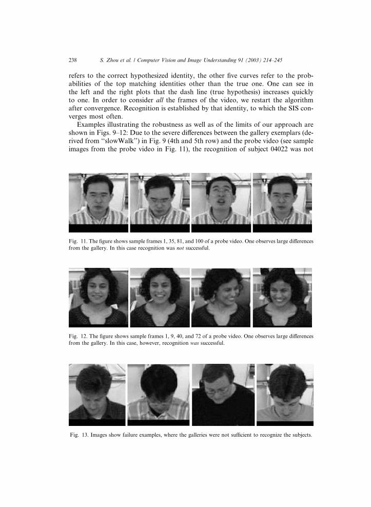
images from the probe video in Fig. 11), the recognition of subject 04022 was not

Fig. 11. The figure shows sample frames 1, 35, 81, and 100 of a probe video. One observes large differences

from the gallery. In this case recognition was not successful.

Fig. 12. The figure shows sample frames 1, 9, 40, and 72 of a probe video. One observes large differences

from the gallery. In this case, however, recognition was successful.

Fig. 13. Images show failure examples, where the galleries were not sufficient to recognize the subjects.


successful (Fig. 10, top). On the other hand, in spite of the differences between the

gallery exemplars and the probe video, subject 04079 was always recognized success-

fully (Fig. 10, bottom).

The major problems that we encountered during our experiments are:

1. Subjects appear significantly different in the gallery video and in the probe videos:This was the case for about 50% of the failed experiments.

2. Subjects looked down while walking: This was the case for roughly 10 subjects

(Fig. 13). In some cases, where the subject looked down in the gallery as well

as in the probe, this was not a problem. However, in cases, where this happened

in only either the probe or the gallery (see Fig. 13, left), this led to mis-classifica-

tion.

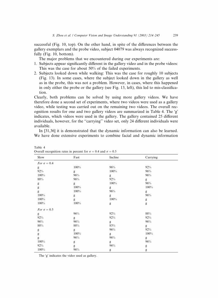
Clearly, both problems can be solved by using more gallery videos. We have

therefore done a second set of experiments, where two videos were used as a galleryvideo, while testing was carried out on the remaining two videos. The overall rec-

ognition results for one and two gallery videos are summarized in Table 4. The �g�indicates, which videos were used in the gallery. The gallery contained 25 different

individuals, however, for the ‘‘carrying’’ video set, only 24 different individuals were

available.

In [31,36] it is demonstrated that the dynamic information can also be learned.

We have done extensive experiments to combine facial and dynamic information

Table 4

Overall recognition rates in percent for r ¼ 0:4 and r ¼ 0:5

Slow Fast Incline Carrying

For r ¼ 0:4

g 100% 96% 92%

92% g 100% 96%

100% 96% g 96%

88% 96% 92% g

g g 100% 96%

g 100% g 100%

g 100% 96% g

100% g g 96%

100% g 100% g

100% 100% g g

For r ¼ 0:5

g 96% 92% 88%

92% g 92% 92%

96% 96% g 96%

88% 88% 83% g

g g 96% 92%

g 100% g 100%

g 96% 96% g

100% g g 96%

92% g 96% g

100% 96% g g

The �g� indicates the video used as gallery.


for recognition. However, we have observed, that the dynamic information of per-

sons can change severely with walking speed. Therefore, we have not included that

information for recognition.

Video images from our test data were converted from color to gray value images,

but no further processing was done. We used throughout our experiments the Eu-clidean distance measure. The set of deformations H included scale and translation.

Shear and rotation were not considered.

7. Discussions and conclusions

We have presented a systematic method for face recognition from a probe video,

compared with a gallery of still templates. A time series state space model is used toaccommodate the video and SIS algorithms provide the numerical solutions to the

model. This probabilistic framework, which overcomes many difficulties arising in

conventional recognition approaches using video, is registration-free and poses no

need for selecting good frames. It turns out that an immediate recognition decision

can be made in our framework due to the degeneracy of the posterior probability of

the identity variable. The conditional entropy can also serve as a good indication for

the convergence. In addition, the still templates in the gallery is generalized to videos

by learning exemplars from the gallery video. However, in order to show that ourapproach is capable of recognizing faces in practice, one needs to work with much

larger face databases.

The following issues are worthy of investigation in the future.

1. Robustness. Generally speaking, our approach is more robust than still-image-

based approach since we essentially compute the recognition score based on all video

frames and, in each frame, all kinds of transformed versions of the face part corre-

sponding to the sample configurations that are considered. However, since we take

no explicit measure when handling frames with outlier or other unexpected factors,recognition scores based on those frames might be low. But, this is a problem for

other approaches too. The assumption that the identity does not change as time pro-

ceeds, i.e., pðntjnt�1Þ ¼ dðnt � nt�1Þ, could be relaxed by having non-zero transition

probabilities between different identity variables. Using non-zero transition proba-

bilities will enable us an easier transition to the correct choice in case that the initial

choice is incorrectly chosen, making the algorithm more robust.

2. Resampling. In the recognition algorithm, the marginal distribution

fðhðjÞt�1;w0ðjÞt�1Þg

Jj¼1 is sampled to obtain the sample set fðhðjÞt ; 1ÞgJj¼1. This may cause

problems in principle since there is no conditional independence between ht and ntgiven z0:t. However, in a practical sense, this is not a big disadvantage because the

purpose of resampling is to �provide chances for the good streams (samples) to am-

plify themselves and hence rejuvenate the sampler to produce better results for future

states as the system evolves� [15]. The resampling scheme can either be simple ran-

dom sampling with weights (like in CONDENSATION), residual sampling, or local

Monte Carlo methods.


3. Computational load. As mentioned earlier, two important numbers affecting the

computation are J , the number of motion samples, and N , the size of the database.

(i) The choice of J is an open question in the statistics literature. In general, larger Jproduces more accurate results. (ii) The choice of N depends on application. Since a

small database is used in this experiment, it is not a big issue here. However, the com-putational burden may be excessive if N is large. One possibility is to use a contin-

uous parameterized representation, say c, instead of discrete identity variable n. Now

the task reduces to computing pðct; htjz0:tÞ. We then can rank the gallery easily using

the estimated ct.4. Now we highlight the differences from Li and Chellappa�s approach [5]. In [5],

basically only the tracking motion vector is parameterized in the state-space model.

The identity is involved only in the initialization step to rectify the template onto the

first frame of the sequence. However, in our approach both tracking motion vectorand identity variables are parameterized in the state-space model, which offers us one

more degree of freedom and leads to a different approach for deriving the solution.

The SIS technique is used in both approaches to numerically approximate the pos-

terior probability given the observation. Again in [5], it is the posterior probability of

motion vector and the verification probability is estimated by marginalizing over a

proper region of state space redefined at each time instant. However, we always com-

pute the joint density, i.e., the posterior probability of motion vector and identity

variable and the posterior probability of identity variable is just a free estimate bymarginalizing over the motion vector. Note that there is no time propagation of ver-

ification probability in [5] while we always propagate the joint density. One conse-

quence is that we guarantee thatP

nt2N pðntjz0:tÞ ¼ 1, but there is no such

guarantee in [5].

Acknowledgments

We thank the three anonymous reviewers for their critical remarks and valuable

suggestions which have considerably improved our paper. The first author would

also like to thank Dr. Baback Moghaddam for helpful discussions.

Appendix A. Derivation of the lower bound for the posterior probability of identity

Suppose that the following two assumptions hold:

• (A) The prior probability for each identity is same,

pðn0 ¼ jjz0Þ ¼ 1=N ; j 2 N ; ðA:1Þ

• (B) for the correct identity l 2 N , there exists a constant g > 1 such that,

pðztjnt ¼ l; htÞP gpðztjnt ¼ j; htÞ; tP 1; j 2 N ; j 6¼ l: ðA:2Þ
Substitution of Eqs. (A.1) and (A.2) into Eq. (6) gives rise to


pðnt ¼ ljz0:tÞ ¼1

N

Zh0

� � �Zht

pðh0jz0ÞYt

s¼1

pðzsjns ¼ l; hsÞpðhsjhs�1Þpðzsjz0:s�1Þ

dht � � � dh0

P1

N

Zh0

� � �Zht

pðh0jz0ÞYt

s¼1

gpðzsjns ¼ j; hsÞpðhsjhs�1Þpðzsjz0:s�1Þ

dht � � � dh0

¼ gt

N

Zh0

� � �Zht

pðh0jz0ÞYt

s¼1

pðzsjns ¼ j; hsÞpðhsjhs�1Þpðzsjz0:s�1Þ

dht � � � dh0

¼ gtpðnt ¼ jjz0:tÞ; j 2 N ; j 6¼ l; ðA:3Þ

where gt ¼Qt

s¼1 g.More interestingly, from Eq. (A.3), we have

ðN � 1Þpðnt ¼ ljz0:tÞP gtXN

j¼1;j 6¼lpðnt ¼ jjz0:tÞ ¼ gtð1� pðnt ¼ ljz0:tÞÞ; ðA:4Þ

i.e.,

pðnt ¼ ljz0:tÞP hðg; tÞ; ðA:5Þ
where
hðg; tÞ ¼ gt

gt þ N � 1: ðA:6Þ

Eq. (A.5) has two implications.

1. Since the function hðg; tÞ which provides a lower bound for pðnt ¼ ljz0:tÞ is mono-

tonically increasing against time t, pðnt ¼ ljz0:tÞ has a probable trend of increase

over t, even though not in a monotonic manner.

2. Since g > 1 and pðnt ¼ ljz0:tÞ6 1,

limt!1

pðnt ¼ ljz0:tÞ ¼ 1; ðA:7Þ

implying that pðnt ¼ ljz0:tÞ degenerates in the identity l for some sufficiently large t.However, all these derivations are based on assumptions (A) and (B). Though it is

easy to satisfy (A), difficulty arises in practice in order to satisfy (B) for all the frames

in the sequence. Fortunately, as we have seen in the experiment in Section 5, numer-

ically this degeneracy is still reached even if (B) is satisfied only for most but not all

frames in the sequence.

More on Assumption (B).

A trivial choice of g is the lower bound on the likelihood ratio, i.e.,

g ¼ inftP 1;j 6¼l;ht2H

pðztjnt ¼ l; htÞpðztjnt ¼ j; htÞ

: ðA:8Þ

This choice is of theoretical interest. In practice, how good is the assumption (B)

satisfied? Fig. 14 plots, against the logarithm of the scale parameter, the �average�likelihood of the correct identity,

1

N

Xn2N

pðInjn; hÞ;

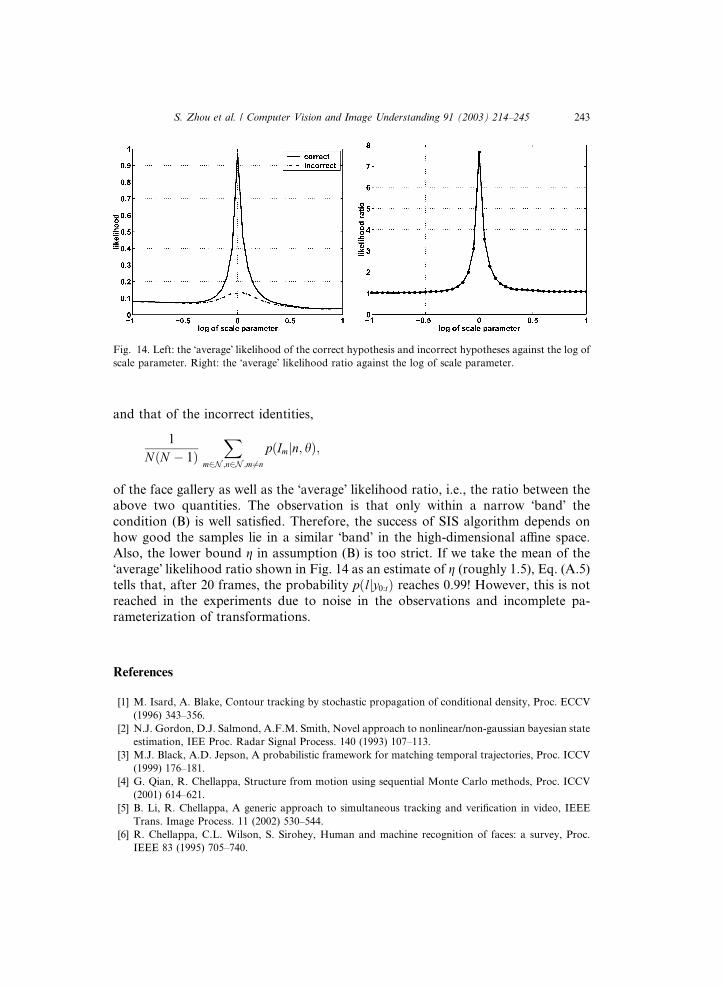
Fig. 14. Left: the �average� likelihood of the correct hypothesis and incorrect hypotheses against the log of

scale parameter. Right: the �average� likelihood ratio against the log of scale parameter.


and that of the incorrect identities,

1

NðN � 1ÞX

m2N ;n2N ;m6¼npðImjn; hÞ;

of the face gallery as well as the �average� likelihood ratio, i.e., the ratio between the

above two quantities. The observation is that only within a narrow �band� thecondition (B) is well satisfied. Therefore, the success of SIS algorithm depends on

how good the samples lie in a similar �band� in the high-dimensional affine space.Also, the lower bound g in assumption (B) is too strict. If we take the mean of the

�average� likelihood ratio shown in Fig. 14 as an estimate of g (roughly 1.5), Eq. (A.5)

tells that, after 20 frames, the probability pðljy0:tÞ reaches 0.99! However, this is not

reached in the experiments due to noise in the observations and incomplete pa-

rameterization of transformations.

References

[1] M. Isard, A. Blake, Contour tracking by stochastic propagation of conditional density, Proc. ECCV

(1996) 343–356.

[2] N.J. Gordon, D.J. Salmond, A.F.M. Smith, Novel approach to nonlinear/non-gaussian bayesian state

estimation, IEE Proc. Radar Signal Process. 140 (1993) 107–113.

[3] M.J. Black, A.D. Jepson, A probabilistic framework for matching temporal trajectories, Proc. ICCV

(1999) 176–181.

[4] G. Qian, R. Chellappa, Structure from motion using sequential Monte Carlo methods, Proc. ICCV

(2001) 614–621.

[5] B. Li, R. Chellappa, A generic approach to simultaneous tracking and verification in video, IEEE

Trans. Image Process. 11 (2002) 530–544.

[6] R. Chellappa, C.L. Wilson, S. Sirohey, Human and machine recognition of faces: a survey, Proc.

IEEE 83 (1995) 705–740.


[7] W.Y. Zhao, R. Chellappa, A. Rosenfeld, P.J. Phillips, Face Recognition: A Literature Survey, UMD

CfAR Technical Report CAR-TR-948, 2000.

[8] P.J. Philipps, H. Moon, S. Rivzi, P. Ross, The feret evaluation methodology fro face-recognition

algorithms, IEEE Trans. PAMI 22 (2000) 1090–1104.

[9] M. Turk, A. Pentland, Eigenfaces for recognition, J. Cognitive Neurosci. 3 (1991) 72–86.

[10] K. Etemad, R. Chellappa, Discriminant analysis for recognition of human face images, J. Opt. Soc.

Am. A (1997) 1724–1733.

[11] P.N. Belhumeur, J.P. Hespanha, D.J. Kriegman, Eigenfaces vs. fisherfaces: recognition using class

specific linear projection, IEEE Trans. PAMI 19 (1997) 711–720.

[12] M. Lades, J.C. Vorbruggen, J. Buhmann, J. Lange, C. von der Malsburg, R.P. Wurtz, W. Konen,

Distortion invariant object recognition in the dynamic link architecture, IEEE Trans. Computers 42

(3) (1993) 300–311.

[13] T. Choudhury, B. Clarkson, T. Jebara, A. Pentland, Multimodal person recognition using

unconstrained audio and video, in: Proceedings of International Conference on Audio- and Video-

Based Person Authentication, 1999, pp. 176–181.

[14] G. Kitagawa, Monte carlo filter and smoother for non-gaussian nonlinear state space models,

J. Comput. Graphical Statistics 5 (1996) 1–25.

[15] J.S. Liu, R. Chen, Sequential Monte Carlo for dynamic systems, J. Am. Statist. Assoc. 93 (1998)

1031–1041.

[16] A. Doucet, S.J. Godsill, C. Andrieu, On sequential Monte Carlo sampling methods for bayesian

filtering, Statist. Computing 10 (3) (2000) 197–209.

[17] R.O. Duda, P.E. Hart, D.G. Stork, Pattern Classification, Wiley-Interscience, New York, 2001.

[18] B. Moghaddam, T. Jebara, A. Pentland, Bayesian modeling of facial similarity, Adv. in Neural

Information Processing Systems 11 (1999) 910–916.

[19] T. Jebara, A. Pentland, Parameterized structure from motion for 3D adaptive feedback tracking of

faces, Proc. CVPR (1997) 144–150.

[20] A. Howell, H. Buxton, Face recognition using radial basis function neural networks, in: Proceedings

of the British Machine Vision Conference, 1996, pp. 455–464.

[21] S. McKenna, S. Gong, Non-intrusive person authentication for access control by visual tracking and

face recognition, in: Proceedings of the International Conference on Audio- and Video-based

Biometric Person Authentication, 1997, pp. 177–183.

[22] H. Wechsler, V. Kakkad, J. Huang, S. Gutta, V. Chen, Automatic video-based person authentication

using the RBF network, in: Proceedings of the International Conference on Audio- and Video-based

Biometric Person Authentication, 1997, pp. 85–92.

[23] J. Steffens, E. Elagin, H. Neven, Personspotter—fast and robust system for human detection,

tracking, and recognition, in: Proceedings of the International Conference on Automatic Face and

Gesture Recognition, 1998, pp. 516–521.

[24] Y. Li, S. Gong, H. Liddell, Modelling faces dynamically across views and over time, Proc. ICCV

(2001) 554–559.

[25] T.M. Cover, J.A. Thomas, Elements of Information Theory, Wiley, New York, 1991.

[26] B. Anderson, J. Moore, Optimal Filtering, Prentice Hall, Englewood Cliffs, New Jersey, 1979.

[27] J. Sullivan, J. Rittscher, Guiding random particle by deterministic search, Proc. ICCV (2001)

323–330.

[28] X. Boyen, D. Koller, Tractable inference for complex stochastic processes, in: Proceedings of the 14th

Annual Conference on Uncertainty in AI (UAI), Madison, WI, 1998 pp. 33–42.

[29] R. Gross, J. Shi, The CMU Motion of Body (MoBo) Database, CMU-RI-TR-01-18, 2001.

[30] B. Moghaddam, Principal manifolds and probabilistic subspaces for visual recognition, IEEE Trans.

PAMI 24 (2002) 780–788.

[31] K. Toyama, A. Blake, Probabilistic tracking in a metric space, Proc. ICCV (2001) 50–59.

[32] B. Frey, N. Jojic, Learning graphical models in images, videos, and their spatial transformations, in:

Proceedings of the Conference on Uncertainty in AI, 2000, pp. 184–191.

[33] D. Lowe, Radial basis function networks, in: M. Arbib (Ed.), The Handbook of Brain Theory and

Neural Networks, 1995, pp. 779–782.


[34] B. Fritzke, Growling cell structures—a self-organizing network for unsupervised and supervised

learning, Neural Learning 7 (1995) 1441–1460.

[35] T. Martinez, K. Schulten, Topology representing networks, Neural Learning 7 (1994) 505–522.

[36] B. North, A. Blake, M. Isard, J. Rittscher, Learning and classification of complex dynamics, IEEE

Trans. PAMI 22 (2000) 1016–1034.

Documents

Probabilistic recognition of human faces from video · Probabilistic recognition of human faces from video q Shaohua Zhou,* Volker Krueger, and Rama Chellappa Center for Automation