Embed Size (px)
Citation preview

RHEINISCH-WESTFÄLISCHE TECHNISCHEHOCHSCHULE AACHEN
KNOWLEDGE-BASED SYSTEMS GROUPPROF. GERHARD LAKEMEYER, PH. D.
Detection and Recognition of HumanFaces using Random Forests for a
Mobile Robot
MASTER OF SCIENCE THESIS
VAISHAK BELLE
MATRICULATION NUMBER: 26 86 51
SUPERVISOR: PROF. GERHARD LAKEMEYER, PH. D.SECOND SUPERVISOR: PROF. ENRICO BLANZIERI, PH. D.
ADVISERS: STEFAN SCHIFFER, THOMAS DESELAERS


Declaration
I declare that this Master Thesis is my own unaided work, except for the official assis-tance from my supervisors. It has not been submitted in any form for any other degreeor diploma at any university or other education institution. Information derived fromthe published or unpublished work of others has been acknowledged in the text and alist of references is included at the end.
Aachen, March 27, 2008
iii


Acknowledgements
I would first like to thank Prof. Gerhard Lakemeyer for an opportunity to work with theKnowledge-based Systems Group. I would then like to express my sincere gratitude toboth Stefan Schiffer and Thomas Deselaers for an incalculable number of suggestions,critical talk and motivational sessions. I owe the entire direction of my thesis to theboth of them. I would like to specially mention the utmost care S. Schiffer has taken onnecessary corrections to my proposal and the final outcome and general advice he hasoffered over the last 8 months.
I would like to thank the AllemaniACs RoboCup team for a great work environmentand putting up with me in general, especially at lunchtimes. I would also like toacknowledge Tim Niemueller for proof-reading the last drafts of the thesis and his sub-sequent suggestions. I thank my friends here in Aachen, who were almost a surrogatefamily and patiently lent their ears to my complaints.
Lastly and most importantly, I dedicate this thesis to my mom, who has been the sourceof constant encouragement. At no point do I except to be able to completely expressthe gratitude I feel towards her.
v


CONTENTS
1 Introduction 11.1 Motivation . . . . . . . . . . . . . . . . . . . . . . . . . . . . . . . . . . . . 11.2 Approach and Contributions . . . . . . . . . . . . . . . . . . . . . . . . . 21.3 Outline . . . . . . . . . . . . . . . . . . . . . . . . . . . . . . . . . . . . . . 3
2 Related Work 52.1 Basic Concepts . . . . . . . . . . . . . . . . . . . . . . . . . . . . . . . . . . 5
2.1.1 Classical Decision Trees and Random Forests . . . . . . . . . . . . 62.2 Image Classification . . . . . . . . . . . . . . . . . . . . . . . . . . . . . . . 72.3 Object Detection . . . . . . . . . . . . . . . . . . . . . . . . . . . . . . . . . 92.4 Segmentation . . . . . . . . . . . . . . . . . . . . . . . . . . . . . . . . . . 92.5 Gesture Recognition . . . . . . . . . . . . . . . . . . . . . . . . . . . . . . 102.6 Summary . . . . . . . . . . . . . . . . . . . . . . . . . . . . . . . . . . . . . 11
3 Face Detection 133.1 Introduction . . . . . . . . . . . . . . . . . . . . . . . . . . . . . . . . . . . 133.2 Approaches To Face Detection . . . . . . . . . . . . . . . . . . . . . . . . . 15
3.2.1 Knowledge-based methods . . . . . . . . . . . . . . . . . . . . . . 153.2.2 Feature-based methods . . . . . . . . . . . . . . . . . . . . . . . . 173.2.3 Template Matching . . . . . . . . . . . . . . . . . . . . . . . . . . . 183.2.4 Appearance-based models . . . . . . . . . . . . . . . . . . . . . . . 193.2.5 Sampling-based Approach . . . . . . . . . . . . . . . . . . . . . . 20
3.3 Discussion . . . . . . . . . . . . . . . . . . . . . . . . . . . . . . . . . . . . 23
4 Face Recognition 254.1 Feature Extraction . . . . . . . . . . . . . . . . . . . . . . . . . . . . . . . . 254.2 Recognition from Intensity Images . . . . . . . . . . . . . . . . . . . . . . 274.3 Databases . . . . . . . . . . . . . . . . . . . . . . . . . . . . . . . . . . . . 32
4.3.1 Training Collections . . . . . . . . . . . . . . . . . . . . . . . . . . 334.3.2 Test Data Collection . . . . . . . . . . . . . . . . . . . . . . . . . . 354.3.3 FERET Protocol . . . . . . . . . . . . . . . . . . . . . . . . . . . . . 36
5 Framework 375.1 Theoretical Foundations of Random Forests . . . . . . . . . . . . . . . . . 37
5.1.1 Decision Trees . . . . . . . . . . . . . . . . . . . . . . . . . . . . . . 37
vii

Contents
5.1.2 Random Forests . . . . . . . . . . . . . . . . . . . . . . . . . . . . . 385.1.3 Generalization Error . . . . . . . . . . . . . . . . . . . . . . . . . . 405.1.4 Conclusion . . . . . . . . . . . . . . . . . . . . . . . . . . . . . . . 41
5.2 Training Data Requirements . . . . . . . . . . . . . . . . . . . . . . . . . . 425.3 Learning Framework . . . . . . . . . . . . . . . . . . . . . . . . . . . . . . 43
5.3.1 Decision Criteria . . . . . . . . . . . . . . . . . . . . . . . . . . . . 435.3.2 Features . . . . . . . . . . . . . . . . . . . . . . . . . . . . . . . . . 445.3.3 Integral Images . . . . . . . . . . . . . . . . . . . . . . . . . . . . . 45
5.4 Growing Trees . . . . . . . . . . . . . . . . . . . . . . . . . . . . . . . . . . 465.5 Face Detection . . . . . . . . . . . . . . . . . . . . . . . . . . . . . . . . . . 515.6 Post Processing . . . . . . . . . . . . . . . . . . . . . . . . . . . . . . . . . 545.7 Face Recognition . . . . . . . . . . . . . . . . . . . . . . . . . . . . . . . . 575.8 Face Learning . . . . . . . . . . . . . . . . . . . . . . . . . . . . . . . . . . 605.9 Parameters . . . . . . . . . . . . . . . . . . . . . . . . . . . . . . . . . . . . 615.10 Implementation . . . . . . . . . . . . . . . . . . . . . . . . . . . . . . . . . 63
5.10.1 Overview . . . . . . . . . . . . . . . . . . . . . . . . . . . . . . . . 635.10.2 Software Architecture . . . . . . . . . . . . . . . . . . . . . . . . . 65
6 Evaluations 696.1 Face Detection . . . . . . . . . . . . . . . . . . . . . . . . . . . . . . . . . . 69
6.1.1 Introduction . . . . . . . . . . . . . . . . . . . . . . . . . . . . . . . 696.1.2 ROC Curve Plots . . . . . . . . . . . . . . . . . . . . . . . . . . . . 71
6.2 Face Recognition . . . . . . . . . . . . . . . . . . . . . . . . . . . . . . . . 776.2.1 Testing Framework . . . . . . . . . . . . . . . . . . . . . . . . . . . 776.2.2 Rank-1 Recognition Rates . . . . . . . . . . . . . . . . . . . . . . . 796.2.3 Unknown Identity . . . . . . . . . . . . . . . . . . . . . . . . . . . 846.2.4 Forest Size . . . . . . . . . . . . . . . . . . . . . . . . . . . . . . . . 866.2.5 KBSG Face Database . . . . . . . . . . . . . . . . . . . . . . . . . . 87
6.3 Summary . . . . . . . . . . . . . . . . . . . . . . . . . . . . . . . . . . . . . 87
7 Conclusion and Future work 897.1 Conclusions . . . . . . . . . . . . . . . . . . . . . . . . . . . . . . . . . . . 897.2 Future Work . . . . . . . . . . . . . . . . . . . . . . . . . . . . . . . . . . . 91
8 Notation 93
Bibliography 95
viii

1 INTRODUCTION
In this master thesis, we present a new framework for the automatic detection, recog-nition and learning of human faces with random forests. The principal motivation forour work is towards the design of a fast face processing system, especially applicable tomobile robots. Given a high amount of social interaction between a robot and humanbeings, the experience is rendered more natural if the robot is able to detect faces andrecognize corresponding identities. If the identity of the person is not known then it islearnt by the robot.
1.1 Motivation
Robots that interact with humans, such as rescue robots and service robots, frequentlyencounter human faces. Rescue robots are principally designed to be of aid to rescueworkers and humans in danger. Typically scenarios where rescue robots are deployedinclude disaster-struck areas, explosions, infernos and building collapses. The robotsself navigate in hazardous environments to either probe for surviving humans or toneutralize any immediate danger and make the surrounding less perilous for humanrescue workers.
Service robots, generally, are designed to offer assistance to humans and to peoplewith disabilities, in particular. They could be used for day to day activities, such asretrieving tools and objects, for and by humans (civil usage). They could also be usedto provide feedback on approaching entities to the visually impaired and in general,provide structural support for the physically or mentally impaired.
In both of the applications of robotics discussed above, there is a high amount of socialinteraction between the robots and the human beings. The robots respond dynamicallyto requests and communicate with human beings. An indispensable characteristic ofsuch robots is the automatic detection and recognition of the faces of humans theyinteract with. To elucidate further, the interaction will be rendered more human-like ifa robot is able to identify a human from a group of known individuals. Further, if theidentification fails then the robot may introduce itself like any of us. It must then learnthe new individual and assimilate the identity into its recognition system. We proposea face processing system that targets the aforementioned requirements.
1

1 Introduction
1.2 Approach and Contributions
Central to our approach are random forests. Random forests are defined as "a combi-nation of tree predictors such that each tree depends on the values of a random vectorsampled independently and with the same distribution for all the trees in the forest" [1].In our thesis, we present an integrated framework to the detection, recognition andlearning of human faces using random forests. Such a system will find immediateapplications in rescue and service robotics as outlined above.
As emphasized, the focal point of our work is towards an improved human-robotinteraction. An important criterion for a prospective face recognition system is responsetime. A robot that reciprocates with a massive delay, at least in relative comparison tohuman beings, will deliver a frustrating experience. A robot that requires an extensiveperiod of time to learn and recognize people is an antithesis to our expectations. Itis thus clear that service robots that accompany the elderly and disabled are to be ofassistance to their owners just as human companions would. It is of essence to have afast face processing system in place.
In line with our contribution to rescue and service robotics, we aim to be applicableto RoboCup@Home. RoboCup@Home is "the largest home robotics competition" andis held annually [2]. This competition is a division of the RoboCup competitions that"attempt to foster AI and intelligent robotics" [3]. RoboCup momentarily encompassesan eclectic collection of games, many of which encourage cooperation between a ma-chine and its human counterpart [4]. The robots are expected to work autonomously.Zant and Wisspeintner [3] discuss tests that outline a few application scenarios. Insome of the scenarios, owner identification is predominant. Learning of new identitiespresent an added improvement in the behavioral component of the robot. Our pro-posal, which presents an integrated framework to detection, recognition and learningof new faces will bring the RoboCup robots closer to the point of succeeding in theabove evaluations.
Contributions to robotics aside, the framework presents an addition to the recent ap-plications of random forests as a statistical learning procedure. Random forests havebeen applied, with promising results, in image classification [5, 6, 7, 8, 9, 10], imagematching [11], positioning discriminatory and generative image regions [12], segmen-tation [13] and gesture recognition [14]. Extending the literature above to developrandom forests for face detection and recognition presents an interesting research goal.Random forests are proven to be fast [12, 5, 6, 7, 8, 9, 10, 15] which is pertinent withour motivation. Further, a random forest is a powerful statistical framework [1] with avery high generalization accuracy. A good generalization accuracy is critical for manylearning algorithms, in general, and image classification in particular as it remarks onthe performance of the algorithm on novel data. Image classification tasks encountersubstantial variations in the image data such as occlusions, illumination variations
2

1.3 Outline
and object pose changes. Our framework effectively casts face detection and recogni-tion as a classification task and hence the aforementioned theoretical benefit of a highgeneralization accuracy is significant.
In general, random forests present the following advantages:
1. The approach is generic. It is easily extendable to the detection and recognitionof any object other than faces.
2. Image classification is reported to be successful in spite of partial occlusions [16].
3. Random forests are a parallel learning algorithm - critical components can beexecuted completely in parallel.
4. The approach has a quick training phase.
5. Random forests can achieve an extremely high generalization accuracy.
6. The nature of random forests presents a uniform strategy for accomplishing manyimage classification tasks.
In conclusion, our goal is to build a fast and unified framework for face detection, facerecognition and face learning using random forests for mobile robots.
1.3 Outline
The outline of the thesis is as follows: Chapter 2 discusses literature on the applicationsof random forests for image classification, object detection, segmentation and gesturerecognition. Chapter 3 reviews the general framework for any face recognition systemand enumerates approaches to face detection. Chapter 4 presents feature extraction,face recognition and publicly available training data for face detection and recognition1.Chapter 5 discusses our framework: face detection, recognition and learning usingrandom forests. Chapter 6 presents comparative evaluations on our approach. Wedraw our conclusions and outline future work in Chapter 7.
1Although our organization of related work in Chapter 2 is limited to applications of random forests, itshould be noted that the face detection and face recognition approaches reviewed are also relevant asrelated work. Chapter 2 only presents frameworks analogous to our own.
3


2 RELATED WORK
In this chapter, we review literature that use random forests for a number of relatedimage classification tasks. The approaches enumerated below, in addition to our work,grow decision trees by randomizing the decision criteria. In Section 2.1, we introducea few basic concepts of a learning framework followed by an overview of classicaldecision trees and random forests.
The literature review, in Section 2.2-2.5, covers applications of random forests to imageclassification, object detection, segmentation and gesture recognition. The applicationsadditionally reveal some of the advantages of random forests. We conclude this reviewin Section 2.6.
2.1 Basic Concepts
A supervised learning system is characterized by a learning algorithm and labeledtraining data [17]. The algorithm dictates a process of learning from information ex-tracted, usually as feature vectors, from the training data.
Training data is typically of the form:
D =!"
!n, cp#
: n = 1, . . . , N; p = 1, . . . , P$
(2.1)
where !N1 are the data and cP
1 are the corresponding class labels. If the training data areimages then the data is considered to be M dimensional, i.e. the images are defined byK! L pixels (where K " L = M). As we work only with images in this work, we limitour discussions to the same.
Any rectangular region of an image is a local characteristic of the image and is referredto as a local visual descriptor [12]. As images, in general, are high dimensional thedescriptors are quantized as feature vectors using filters. Feature vectors are a moreefficient representation for purposes of comparisons and computations by the learningframework.
A general description of a filter is given by,
f (!) : ! #$ %M&(2.2)
5
2 Related Work
where M& < M and % is the space of real numbers. Essentially, a filter maps an imageor a region to either a scalar (M& = 1) or a vector (characterized by dimensions lowerthan M). The resulting entity is termed as a feature or a feature vector respectively.
A learning framework uses the feature vectors extracted from the labeled training datato build a classifier for classification. The task of classification is to assign a label onnovel data given labeled training data.
A general definition of a classifier is given by,
h(!) : ! #$ p (2.3)
where p = {1, . . . , P} is the class label awarded to the novel image !. To investigatethe performance of a learning framework, we use a labeled test data collection thatmeasures the accuracy of the labels awarded. Formally, classifier accuracy is probedwith a correctness indicator function Ih(!) defined as,
Ih(!) =%
1 if h(!) is the true label of the test image !0 otherwise (2.4)
2.1.1 Classical Decision Trees and Random Forests
A random tree is structurally homogenous to a classical decision tree. Classical decisiontrees and random trees are grown recursively top down. Classical decision trees find adecision criterion that best divides the multi-class training data into two groups at eachnode [18]. A decision criterion consists of an attribute and a related threshold.
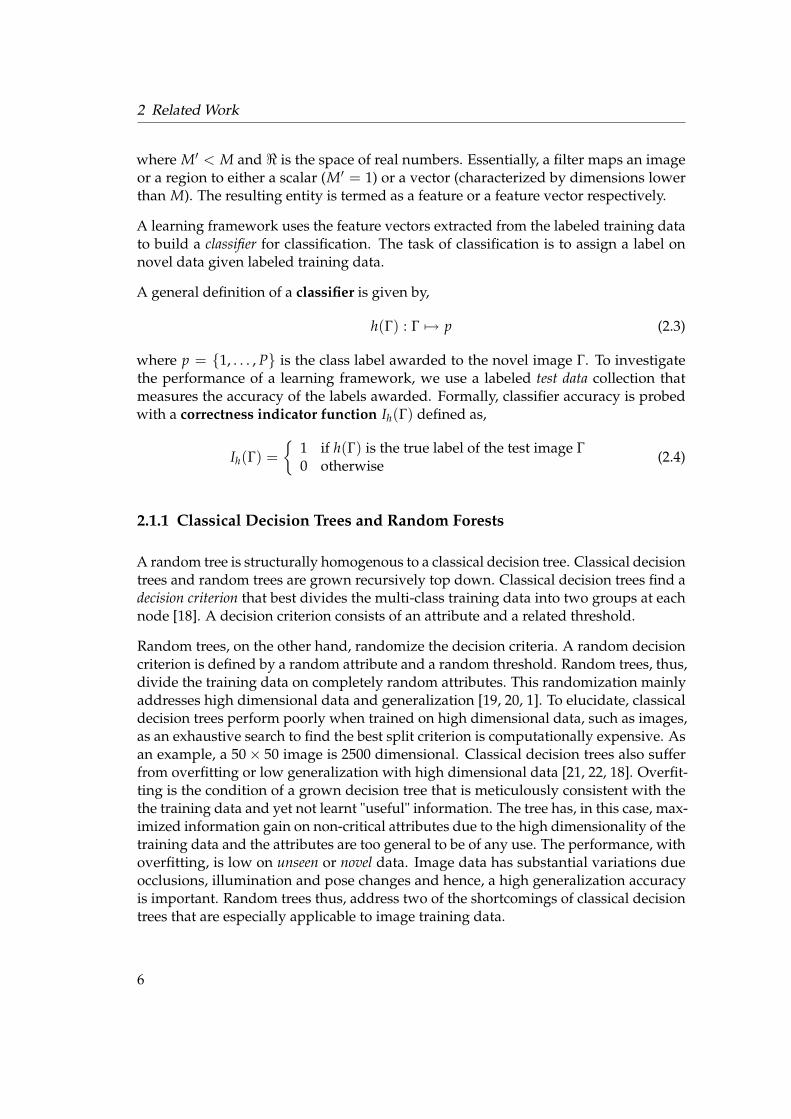
Random trees, on the other hand, randomize the decision criteria. A random decisioncriterion is defined by a random attribute and a random threshold. Random trees, thus,divide the training data on completely random attributes. This randomization mainlyaddresses high dimensional data and generalization [19, 20, 1]. To elucidate, classicaldecision trees perform poorly when trained on high dimensional data, such as images,as an exhaustive search to find the best split criterion is computationally expensive. Asan example, a 50! 50 image is 2500 dimensional. Classical decision trees also sufferfrom overfitting or low generalization with high dimensional data [21, 22, 18]. Overfit-ting is the condition of a grown decision tree that is meticulously consistent with thethe training data and yet not learnt "useful" information. The tree has, in this case, max-imized information gain on non-critical attributes due to the high dimensionality of thetraining data and the attributes are too general to be of any use. The performance, withoverfitting, is low on unseen or novel data. Image data has substantial variations dueocclusions, illumination and pose changes and hence, a high generalization accuracyis important. Random trees thus, address two of the shortcomings of classical decisiontrees that are especially applicable to image training data.
6

2.2 Image Classification
To reiterate our description, a random tree selects a random feature and a randomthreshold and divides the training images at a node. Recursively, a complete tree andsubsequently a collection of trees are built that constitute a random forest. The classi-fication results from each tree are collected for an input image and typically, a simplemajority voting scheme awards the resulting class label. In the following sections, wepresent the use of random forests on a number of related image classification tasks.
2.2 Image Classification
Random forests for image classification have been extensively covered by Marée etal [5, 6, 9, 10]. A general description of the image classification problem is to categorizea previously unseen input image and subsequently assign a label using informationdrawn from labeled training images [10]. Image classification is used with images fromgeology, biology, building images, cars, motorbikes etc. for various labeling tasks.
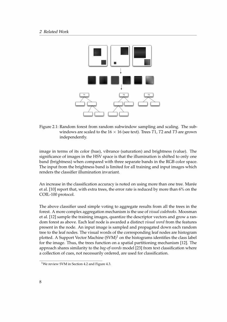
The central idea of the approach taken by Marée et al. [10] is to sample random sub-windows, scale them and grow a random forest from features extracted from the sub-windows. The sampled subwindows are random both in their location and size. Thesize is allowed to range between 1 ! 1 pixels to the maximum square window possible.Once sampled, the subwindows are rescaled to 16 ! 16 pixels.
An illustration ensues in Figure 2.1. Here, numerous subwindows, of different sizes,are sampled and account for decisions at different levels of a tree. The textures inthe figure represent local patterns. Three random trees are shown, each of whichis built independently. The trees necessarily need to be built independently as thegeneralization error is inversely proportional to the independence of the trees [1].
Classification on an input image is carried out by randomly extracting subwindowsin the image and propagating scaled subwindows down each tree in the forest. Votesfrom each of the random trees for all sampled subwindows are aggregated. A simplevoting scheme with majority ruling awards the corresponding class label. Experimen-tal evaluations on a variety of image classification databases, namely (i) COIL-100, adataset of 100 different 3D objects, and (ii) ZuBuD, a dataset of 201 buildings in Zürichwere presented. The results are very competitive.
Marée et al. [9] discuss that one of the benefits of the random forest approach is thatthe classification is robust to partial occlusions. This is attributed to the fact that not allthe sampled subwindows of the input image need to be correctly labeled. The votingscheme allows the classifier sufficient flexibility to falsely categorize a few subwin-dows.
Marée et al. [5, 10] also claim that the rescaling of all sampled subwindows to a fixeddimension for training renders the classifier scale invariant. Further, the pixel valuesare moved to the Hue-Saturation-Value (HSV) space. The HSV value considers the
7
2 Related Work
T1 T2 T3
Figure 2.1: Random forest from random subwindow sampling and scaling. The sub-windows are scaled to the 16 ! 16 (see text). Trees T1, T2 and T3 are grownindependently.
image in terms of its color (hue), vibrance (saturation) and brightness (value). Thesignificance of images in the HSV space is that the illumination is shifted to only oneband (brightness) when compared with three separate bands in the RGB color space.The input from the brightness band is limited for all training and input images whichrenders the classifier illumination invariant.
An increase in the classification accuracy is noted on using more than one tree. Maréeet al. [10] report that, with extra trees, the error rate is reduced by more than 6% on theCOIL-100 protocol.
The above classifier used simple voting to aggregate results from all the trees in theforest. A more complex aggregation mechanism is the use of visual codebooks. Moosmanet al. [12] sample the training images, quantize the descriptor vectors and grow a ran-dom forest as above. Each leaf node is awarded a distinct visual word from the featurespresent in the node. An input image is sampled and propagated down each randomtree to the leaf nodes. The visual words of the corresponding leaf nodes are histogramplotted. A Support Vector Machine (SVM)1 on the histograms identifies the class labelfor the image. Thus, the trees function on a spatial partitioning mechanism [12]. Theapproach shares similarity to the bag-of-words model [23] from text classification wherea collection of cues, not necessarily ordered, are used for classification.
1We review SVM in Section 4.2 and Figure 4.3.
8

2.3 Object Detection
2.3 Object Detection
Image matching extends image classification and can be used to detect "objects" in abackground. The problem can be defined as follows: given knowledge of the geometricappearance of an object, followed by a few scenes of the object in a background, objectdetection identifies the extent and the position of objects, if any, in an input image [16].The presence of objects in the input image is as determined by a human.
Figure 2.2: Selection of a few hundred keypoints in an object [11].
Lepetit et al. [11] present a selection of 200 keypoints based on a probability measure.Figure 2.2 shows the selection of such keypoints in a stuffed toy. A random tree isgrown by creating tests at nodes of the kind: is the intensity of the pixel at (x, y) higherthan the intensity of the pixel at (x + 1, y)? Forests are grown by using random subsetsof the training images for each tree to ensure increased independence between thetrees. To detect the object, patches of the input image are propagated down the treeand keypoints are matched.
2.4 Segmentation
Yin et. al [13] present a random forest based monocular segmentation approach. Theprincipal application targeted is video chat with background substitution. Segmenta-tion is defined as the separation of an object of interest from its background. While themost competitive results to segmentation have been achieved with stereo vision [24],comparable results are presented using monocular vision and random forests.
Spatio-temporal derivates are used as "motion" filters. The filters are clustered andtitled as motons. Each moton represents a unique response of input images (imagesfrom the video camera) to motion analysis. For instance, image regions that "move" inthe background are identified with clustered spatio-temporal derivates as the "movingedge" moton. Regions of an image with weak textures are identified with a "weak
9
2 Related Work
texture" moton. Regions of the image that do not move are identified with a "stationary-edge" moton.
Rectangular regions sampled from captured still images are paired with motons asshape filters. The shape filters are used in training random forests. A subset of shapefilters are used to train each tree. Training with subsets of shape filters guarantees inde-pendence between the random trees. An approach previously discussed in Section 2.3also train random trees with subsets to ensure independence.
When the video chat is initiated, a captured image is propagated down each tree.The shape filters segment the foreground from the background. The latter is thensubstituted with any other image.
2.5 Gesture Recognition
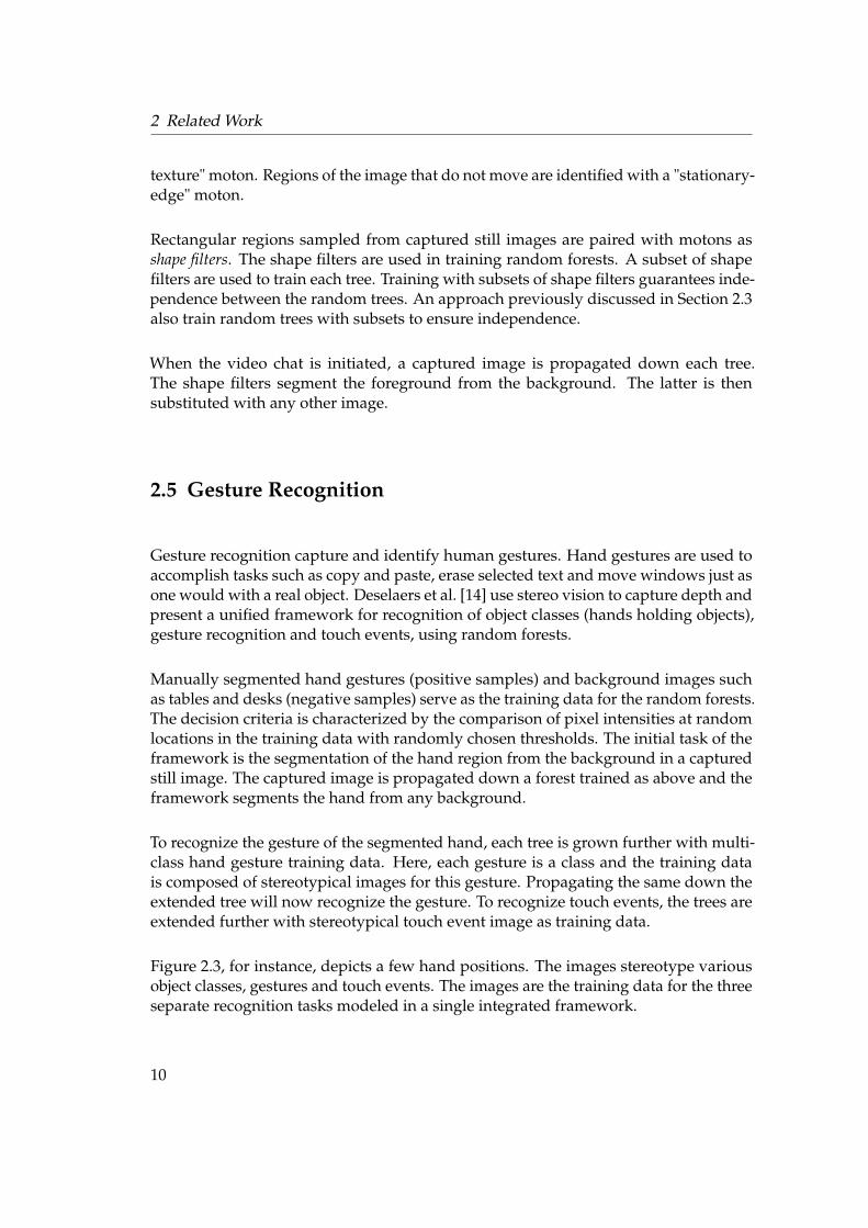
Gesture recognition capture and identify human gestures. Hand gestures are used toaccomplish tasks such as copy and paste, erase selected text and move windows just asone would with a real object. Deselaers et al. [14] use stereo vision to capture depth andpresent a unified framework for recognition of object classes (hands holding objects),gesture recognition and touch events, using random forests.
Manually segmented hand gestures (positive samples) and background images suchas tables and desks (negative samples) serve as the training data for the random forests.The decision criteria is characterized by the comparison of pixel intensities at randomlocations in the training data with randomly chosen thresholds. The initial task of theframework is the segmentation of the hand region from the background in a capturedstill image. The captured image is propagated down a forest trained as above and theframework segments the hand from any background.
To recognize the gesture of the segmented hand, each tree is grown further with multi-class hand gesture training data. Here, each gesture is a class and the training datais composed of stereotypical images for this gesture. Propagating the same down theextended tree will now recognize the gesture. To recognize touch events, the trees areextended further with stereotypical touch event image as training data.
Figure 2.3, for instance, depicts a few hand positions. The images stereotype variousobject classes, gestures and touch events. The images are the training data for the threeseparate recognition tasks modeled in a single integrated framework.
10
2.6 Summary
Figure 2.3: A set of sample hand positions stereotypical of clutching objects (pen, paper,card) and actions (grab, select). [14].
2.6 Summary
As discussed previously, the approaches are, in principle, analogous image classifi-cation tasks. The exact nature of the training data used is dependent on the specificgoal of the learning framework. The decision criterion in every approach enumeratedin this review is characterized by a random component. Marée et al. [9, 5, 6, 10] andMoosmann [12] sample rectangles of random dimension at random locations. Lepetitet al. [11] sample pixels at random locations. Yin et al. [13] randomly sample shapefilters, defined as clustered spatio-temporal operators paired with rectangular regions.Deselaers et al. [14] sample pixels at random locations. Subsequent to the growth ofthe forest, the classification tasks sample the input images and propagate the same onthe trees to return class labels. In our own framework, the random component is thesampling of randomly sized rectangles at random locations from the training data. Theframework is presented ensuing a review of the current approaches to face detectionand face recognition.
11


3 FACE DETECTION
As Yang et al. [25] discuss, research in face recognition proceeds with the assumptionthat the face is already segmented from the background image. However, a completeface processing system must include an additional face detection system that is ableto segment or extract faces from a complex background and supply the faces to arecognition module.
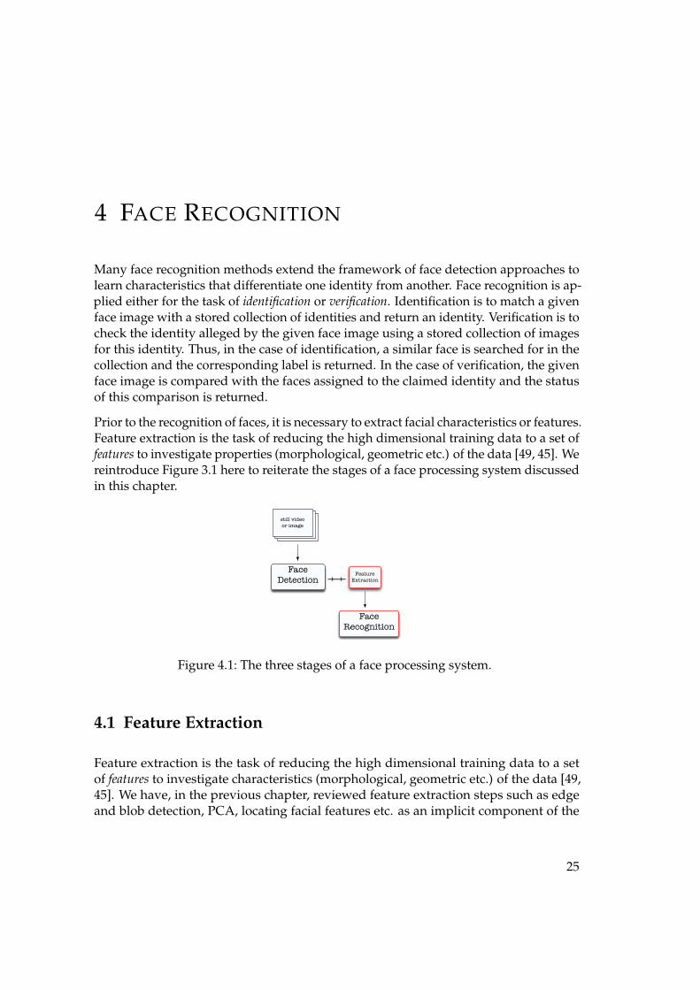
An intermediary stage is that of extracting features. As many face detection approachestrain on features, feature extraction may be an implicit component in the system. Fig-ure 3.1 shows the three stages of face recognition. In this chapter, we discuss ap-proaches to face detection.
still video
or image
FaceDetection
Face Recognition
Feature
Extraction
Figure 3.1: The three stages of a face processing system.
3.1 Introduction
Face recognition systems are currently one of the most important and widely usedapplications of image understanding and pattern recognition [26]. Some commonapplications include,
• Service and Rescue Robots: offer assistance, neutralize perilous environments,structural support to the disabled.
• Biometrics: driver’s license, passports and voter registrations.
• Information Security: file encryption and desktop logon.
• Law Enforcement and Surveillance: CCTV cameras and suspect tracking.
13

3 Face Detection
• Access Control: facility access (access to buildings and houses).
In the above, face images serve as the primary input to accomplish tasks of encryptionand identification. We note that applications such as suspect tracking might haveto deal with different head gaits, partial occlusion of the faces due to foreign objectsamong others. Even a desktop logon system can expect the presence of a foreign bodyin the background as can a facility access provider. None of these applications can thusstraightforwardly carry out face recognition. The crucial step is to precisely locate thefaces in the image prior to further processing. This step is referred to as face detection.Face detection is thus defined as, “Given an arbitrary image, the goal of face detectionis to determine whether or not there are any faces in the image and, if present, returnthe image location and extent of each face” [25].
A face detection system, operating in real life scenarios, can be expected to encounterany of the challenges listed below. For instance, a service robot and its supportingcamera usually captures furniture, different light sources, other objects along withhumans.
• Pose variations. Excluding the sole case of a human facing the camera either outof participation or accident, most applications can expect different side profiles.Some applications, such as a smaller robot interacting with a human, capture stillimages from a lower angle. CCTV Cameras usually capture human faces froman upper angle. In rare cases, upside down and rotated faces are also captured.
• Occlusions. Foreign objects obstructing the view of the camera make the taskof detection (and recognition) difficult. Depending on the percentage of the facethat is occluded, face detection may even be impossible.
• Illumination. Another challenge is related to the illumination conditions underwhich the image was obtained. For instance, if the illumination was very low, theface contour might not be discernible from the background. Only a part of theface may be illuminated. Further, the source and direction of the illumination isalso important.
• Facial components and structures. The presence or absence of beards and mus-taches, changed hair styles are also challenges.
In most real life scenarios, a captured image includes multiple faces. A simplified prob-lem is, thus, to assume the presence of only one human face in the input image. This isreferred to as the face localization problem. An alternative is the task of locating features,such as eyes, nose, ears and mouth, and is referred to as facial feature detection.
A measure of the effectiveness of a face detection system is the detection rate. Thedetection rate is calculated as,
Detection rate =Number of faces correctly detected
Total number of faces in the image as determined by a human
14

3.2 Approaches To Face Detection
where the rate is derived from the generic correctness indicator function previouslydefined in Equation 2.4.
A detection stage can commit two kinds of errors: false positives and false negatives [25].False positives are referred to as those errors when a face was reportedly detected bythe system but there is no face in the image. A false negative is recorded in case aface is not detected, i.e. a region of the input image is falsely assumed to not contain aface. Further, awarding the "bounding box" returned to be a correctly detected face isdetermined by constrains that declare the percentage of overlap between the returnedbounding box and the actual face as a threshold. Additionally, the extent of the face(area of the bounding box) independently is measured to the extent as determined bya human being. If the bounding box is too large or too small, then the result is deemedas invalid.
The granularity of false positives and negatives can be reviewed further with the align-ment error. The alignment error is the case of a subwindow nominated as a face, butthe position and extent of the detection only partly covers the face. Depending on theprecision expected of the detections, the alignment errors border false positives or falsenegatives. We note that procuring very high detection rates with an increasing num-ber of false positives is not a fair evaluation, i.e. the false positives count is almost asimportant as the detection rate. Algorithms search for a tradeoff between the detectionrate and the number of false positives. A graphical tool that monitors this tradeoff isthe Receiver Operating Characteristics (ROC) curve [27, 28].
It can be concluded from the above that face detection, as a machine learning ap-proach, is a two class problem: the task is to identify if an image region is a “face” ora “non-face”. In accordance, the training data for face detection is organized into twocollections: faces and background images. In the following section, we review a fewapproaches to face detection.
3.2 Approaches To Face Detection
Traditionally, the approaches to face detection can be roughly divided into four cat-egories: knowledge-based, feature-based, template matching and appearance-based.Recent literature [29, 30], including our work, utilize a generic sampling-based ap-proach. We review all five categories in this section.
3.2.1 Knowledge-based methods
Knowledge-based methods extrapolate the human understanding of the structuralcharacteristics of a face. Rules are formalized from morphological facts. The presenceof two eyes which are symmetrical, a triangular nose, the relative difference in color
15
3 Face Detection
between parts of the human face etc. are encoded as relationships. If the rules encodedare too specific, the detection accuracy drops as small variations in the requirementsresults in false negatives. If the rules are too general, many false positives result. Toallow for variations in the structural descriptions, a few approaches employ fuzzytheory.
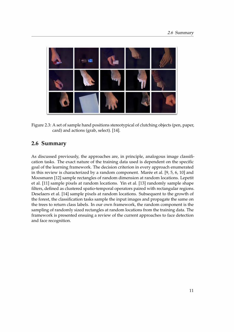
The approach typically builds on multi-resolution or mosaic images. Initially, imageanalysis is carried out at a very low resolution to probe for any high level morphologi-cal description. Subsequently, the resolution is increased and the descriptions are morespecific.
hair
beard
Figure 3.2: Structural characteristics are encoded as rules in different cells. The diagramdepicts a " shaped hair region, a beard region and central homogenous noseand mouth region [31].
Yang and Huang [32] divide a stereotypical face into a number of units or cells thatmust conform to specified descriptions as shown in Figure 3.2. In the figure the centralregion of the face, for instance, occupy 4 ! 4 cells. This is referred to as a quartet. Thebottom portion of this quartet occupies 4 cells (light gray colored) and typically, thisregion of a face is homogeneously colored. Thus, a rule that applies here is “this part ofthe face has four cells with a basically uniform intensity”. Similarly, a "-shaped regioncomposed of dark pixels and of significant length denotes a stereotypical hair area. Astereotypical beard description is depicted in the figure as well.
At a higher resolution, the quartet is subdivided into 2 ! 2 regions or octets. With ananalogous rule description, the eyes and nose are detected. The approach is thus a hi-erarchical knowledge-based recognition system [32, 31, 25]. Kotropoulos and Pitas [31]extend the work by reducing computational needs and a preprocessing step to estimatecell dimensions.
16
3.2 Approaches To Face Detection
The importance of this technique is the modeling of human intuition although it suffersfrom being more of a localization technique as opposed to detection of multiple faces.
3.2.2 Feature-based methods
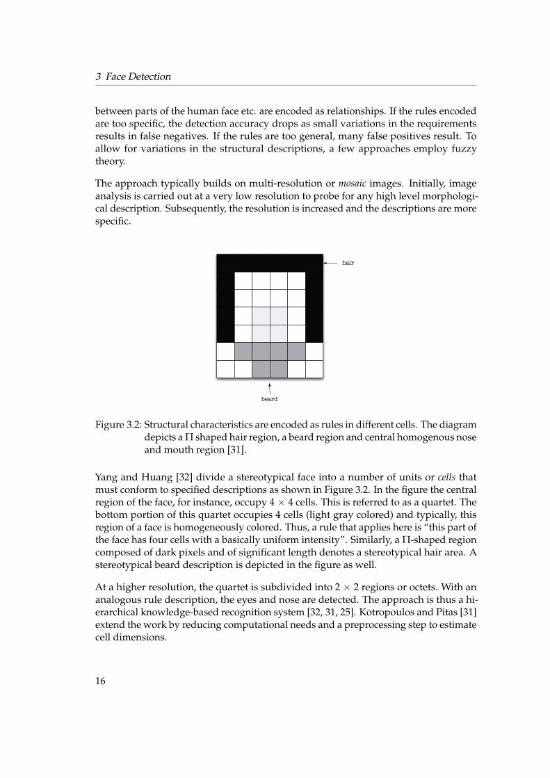
Feature-based methods are those that take a bottom-up approach by locating facialfeatures initially and then collecting their respective enclosing entities such as edges,blobs, streaks and graphs as a detected face. Typically, edge detectors are used toidentify particular shapes such as eyebrows, eyes, noses etc. and statistical modelsestimate distances between these shapes. A linking stage follows that collects theminto groups and subsequently detects a face. Figure 3.3 illustrates this approach: edgefiltering and grouping to detect faces.
Eyebrows Eyes Nose
Linking
Figure 3.3: Edge detection followed by linking and grouping to detect faces.
Sirohey [33] reasons that since the shape of a face is roughly elliptical, facial features canbe combined in an ellipse fitting probe. Essentially, he uses a Canny Edge Detector1 [34]to identify all the edges. Heuristics are used to create an edge map, i.e. unconnectededges (the output of the edge detector) are linked to verify if ellipses formed thusconform to that of a face contour. The final result is a detected face.
While Sirohey uses edges of face features and face contours, any sort of morphologicalidentity can be chosen. For instance, learning the texture of skin and hair is usedto detect faces [25]. The use of skin color in color spaces, such as RGB and HSV, toaccomplish detection is also reported [35].
Graf et al. [36] use a combination of features to detect faces from videos. Their approachuses shape modeling, color response and motion. The first stage uses spatial frequencyfilters to identify the best set of facial features (eyes, nose etc.) that can be used to
1A Canny Edge Detector is an multi-stage detection technique. A complete description of the techniqueis beyond the scope of this thesis.
17

3 Face Detection
detect faces. The second stage trains on the best thresholds for responses to color filtersthat can segment faces from the background. The last stage calculates the absolutedifference in regions to identify "moving" pixels to segment the human face. This issimilar to a spatio-temporal filter. The three different stages supply a list, as cues, and an-gram2 model decides on the location and extent of a face. Feature-based approaches,in general, perform poorly with blurred images [25].
3.2.3 Template Matching
Template matching is based on correlation values. Features such as contours and edgesare extracted and their relative locations are matched against predetermined estimates.Conformance to a certain ’skeleton’ is considered to be a detection.
Scassellati [37] uses ratio templates for quick detection of faces. He considers ratiotemplates to be "biologically plausible" as the templates can be hand coded or learntfrom training data, much like the learning models in humans. The approach virtuallydivides the human face into 16 regions of interest using a 14 ! 16 pixels grayscale win-dow. Each region is averaged using a grayscale window. Modeling the typical relativebrightness between the regions, the ratio template outlines constrains for a region to beconsidered to contain a face. The regions also intuitively denote different portions of aface, such as the temple (left or right) and forehead (left or right). Typically, irrespectiveof the illumination conditions, the eyes are darker, the nose is homogeneously brighteretc. thus making ratio templates illumination invariant. Figure 3.4 illustrates the di-visions and relationships in the model. As faces in an input image can occur at manyscales, the grayscale template is probed for all possible regions of the input image atdifferent scales to detect faces.
An improvement to the "fixed" templates, such as the approach above, are deformabletemplates. With deformable templates, sufficient flexibility in the template structureis allowed so as to account for variations and thus increase the detection rate. Theyaddress some of the shortcomings of fixed templates where the latter suffers from lowdetection rates with shape, scale and pose variance.
Yuille et al. [38] propose a generic deformable template based on an energy mini-mization function. The energy function is defined by peaks, edges and valleys corre-sponding to a feature. For instance, they define an eye template characterized by fourproperties, the first of which is a circle of an specific radius that corresponds to theenclosing circle of the iris. The second describes a contour for the eye. The third andfourth model the whites of the eye. The template definitions are built as a functionand the algorithm searches for a conformance to the definitions, i.e. lowest value that
2An n-gram is a probability measure for subsequences. Here, sequences of features from the three stagesthat lead to a detected face in the training data are learnt.
18

3.2 Approaches To Face Detection
1
14
15
432
1312
11
1098
765
16
Figure 3.4: A division of a stereotypical face into 16 regions of interest. The face isassumed to be 14! 16 pixels in dimension. Relationships are encoded todetect faces [37, 25].
the function can achieve, in the input image. Such templates can be extended to otherfeatures and the face itself.
3.2.4 Appearance-based models
Appearance-based models attempt to reduce the dimension of the training data beforeextracting statistical properties. Typically, these models calculate the class-conditionalprobability for a feature vector extracted from the input image. If the feature vector is x,then we calculate the Bayesian likelihoods p(x| f ace) and p(x|non- f ace) from the train-ing data [25]. Since a direct computation of likelihoods is computationally expensivetechniques such as Principal Component Analysis (PCA) are used for dimensionalityreduction.
Eigenfaces [39, 40] is a pioneering appearance-based approach [41]. Let us considerM dimensional training data denoted as !N
1 . PCA attempts to find an effective andefficient representation of the training data. From the training data !1, . . . , !N , theaverage image and the covariance matrix is calculated as,
! =1N
N
#n=1
!n
C =1N
N
#n=1
(!n ' !)(!n ' !)T (3.1)
where ! is the average and C is the covariance.
19

3 Face Detection
The eigensolution for the covariance matrix is calculated and the eigenvectors areordered in decreasing eigenvalues. The eigenvectors considered thus are representativeof the training images where the higher vectors contain most of the information. Toaccount for generative information, a subset of the highest eigenvectors M& (whereM& < M), is used. The cardinality of M& is heuristically chosen. The eigenvectors arecollectively referred to as the "face space" [39].
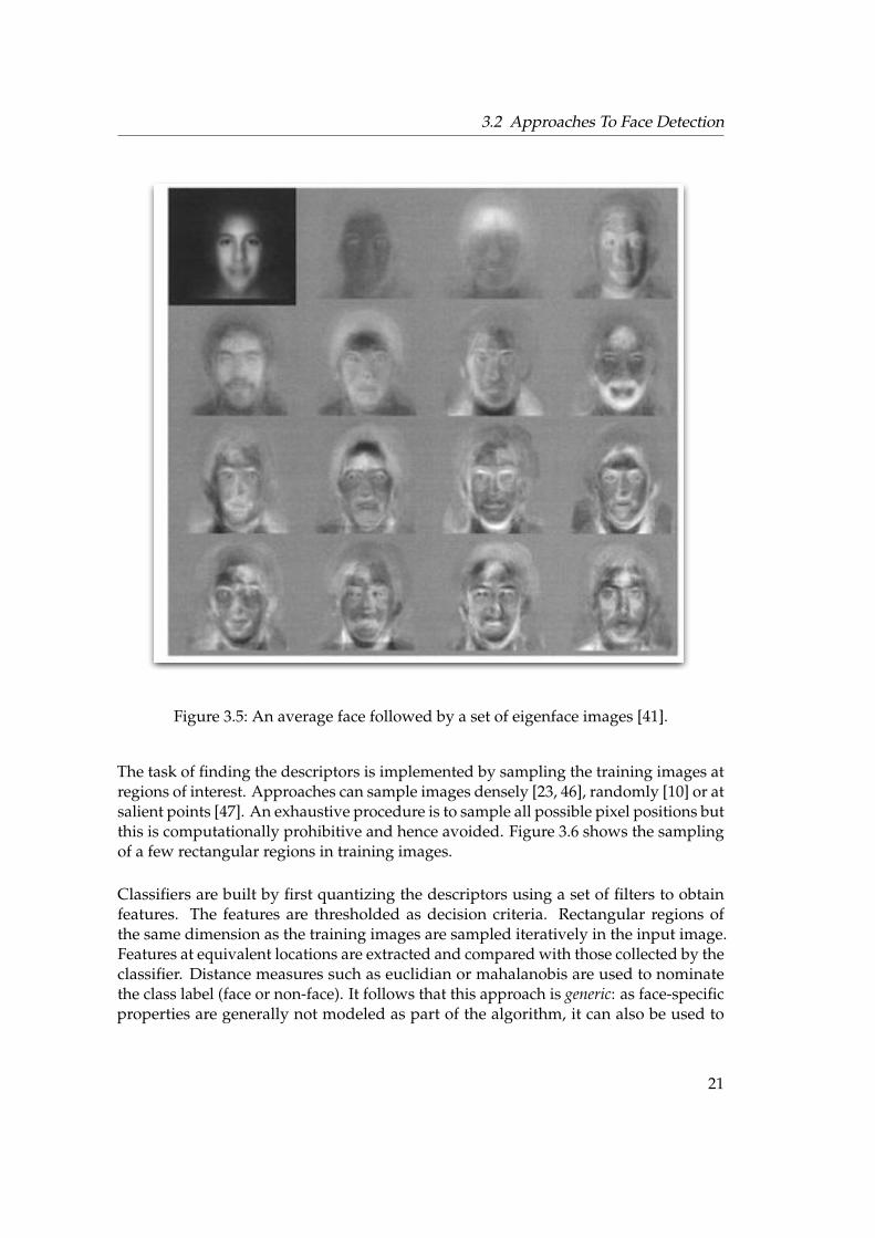
To detect faces, an image region ! of the same dimensions as the training image ismapped to the face space by first calculating !' ! and considering the dimensions inM& only. If a region contains a face, the representation of the same in the "face space"will be small as we calculate the difference with the average face, !, in !' !. Similarly,the "face space" representation for a non-face will be comparatively larger. A thresholdcan thus determine if the region is a face. An iterative procedure over all possiblelocations will return a list of image patches regarded to contain faces by the algorithm.The input image can be scaled to different factors and the procedure repeated to detectfaces of all sizes. Figure 3.5 shows an average face ! and a set of eigenfaces.
Sung and Poggio [42] introduce a distribution-based face detection approach. Canon-ical face and non-face patterns are collected as training images from which represen-tational clusters are listed. The clusters are approximated to a number of multidimen-sional Gaussians. The clusters are further refined by using non-face clusters, also ap-proximated as Gaussians, that surround the face clusters. Distance measures betweenthe collection of clusters detect faces in sampled regions of the input image.
A discussion on appearance based models would be incomplete without a mention ofthe neural network based face detection system by Rowley et al. [28, 43]. An ensembleof neural networks trained on preprocessed images is used. Training images are 20 !20 pixels in dimension and are histogram equalized3 so as to render the system illu-mination invariant. To deal with the false positives, a number of arbitration methodssuch as an attentional neural network to merge detection results from different neuralnetworks are employed. If faces are falsely detected in images where there are none,the regions assumed to contain faces are added to the non-face training image collec-tion so as to prevent such detections in the future. The end result is a very robust facedetection framework. To conclude, we note that appearance-based methods remain tooffer one of the most competitive results to-date.
3.2.5 Sampling-based Approach
Sampling-based approaches probe local visual descriptors to learn facial characteristics.In contrast to some of the previous approaches, the descriptors are estimated directlyfrom the training data and do not typically conform to any template.
3Histogram equalization is an image processing technique to modify the dynamic range of image inten-sities and improve contrasts [44, 45].
20
3.2 Approaches To Face Detection
Figure 3.5: An average face followed by a set of eigenface images [41].
The task of finding the descriptors is implemented by sampling the training images atregions of interest. Approaches can sample images densely [23, 46], randomly [10] or atsalient points [47]. An exhaustive procedure is to sample all possible pixel positions butthis is computationally prohibitive and hence avoided. Figure 3.6 shows the samplingof a few rectangular regions in training images.
Classifiers are built by first quantizing the descriptors using a set of filters to obtainfeatures. The features are thresholded as decision criteria. Rectangular regions ofthe same dimension as the training images are sampled iteratively in the input image.Features at equivalent locations are extracted and compared with those collected by theclassifier. Distance measures such as euclidian or mahalanobis are used to nominatethe class label (face or non-face). It follows that this approach is generic: as face-specificproperties are generally not modeled as part of the algorithm, it can also be used to
21

3 Face Detection
Figure 3.6: Sampling rectangular regions for training [48].
detect objects other than faces.
A renowned [29] sampling-based learning framework was proposed by Viola andJones [30] that uses boosting to learn discriminant features4. This approach buildsmany binary decision stages. Each stage focuses on features that leads to the minimalerror on dividing the training set into two groups. Since there is usually never a singlefeature that returns zero error [30], the learning algorithm builds attentional stageson features that return the minimal error for each additional stage. At the end of thetraining procedure we obtain a cascade of simple classifiers that have learnt a small setof criteria to effectively determine if a region of the input image contains a face or not.As it is the subject of all our performance evaluations, we briefly review a summary ofthe approach.
For a two-class problem, Equation 2.1 can be written as {(!n, cn) : n = 1, . . . , N}, wherecn ( { f ace, non- f ace} is the corresponding class label. At each stage t, the approachcomputes a classifier that divides the training data at this stage into two with thesmallest error. The error with respect to a classifier hj is evaluated as,
" j = #n
wn|hj(!n)' cn| (3.2)
where hj(!n) is 1 if the feature in !n exceeds the threshold and 0 if not. Equation 3.2thus computes the number of training images that will be misclassified on this classifier.All possible classifiers are considered and the classifier with the lowest " is chosen asht for the stage t.
Initially, the weight wn is set to the same value for every image in !N1 . In subsequent
stages, the weight is influenced by the error calculated in Equation 3.2 for the previousstage as,
wt+1,n = wt,n#1'ent
4Discriminant features of a class are features specific to the class, i.e. features that distinguish this classfrom the others.
22

3.3 Discussion
#t ="t
1' "t(3.3)
where, en is 0 if !n was correctly classified by the classifier and 1 if not. The "t representsthe error with respect to ht.
After T stages, the classifier is given as,
h(x) =
&'(
')1
T
#t=1
$tht(x) ) 12
T
#t=1
$t
0 otherwise,(3.4)
where $t = 1/#t. Subwindows of the same dimension as the training images aresampled from the input image and if the classifier returns 1, then the same is nominatedto be a detected face. The sampling continues at different scales to return all the facesin the input image.
3.3 Discussion
We observe that there is clearly a noticeable overlap between the approaches. Forinstance, edge maps and elliptical structure templates (Sirohey [33]) is also a templatebased approach although it is presented as a feature-based approach. Some approachescan thus be classified into two categories. Further, the boundary between knowledge-based approaches and template-based is also fuzzy [25]. Template-based approachesalso model the human intuition on the morphological characteristics of a human face.
We note that earlier face detection approaches suffered from the inability to detect facesof different scales and side profiles. Detecting differently sized faces in the same inputimage have since been addressed by many [28, 43, 30, 42, 25].
Typically, to detect faces in the input image, a detection framework uses the slidingsubwindow approach. Image patches (subwindows) are sampled, iteratively, from theleft to right and top to bottom. The dimension of the subwindow is equal to the dimen-sion of faces in the training images. Effectively, the sliding window finds subwindowssimilar to the images that the framework was trained on. The face detector returns aface or a non-face label for the sampled subwindow. Similarly, the iterative samplingroutine lists all subwindows nominated to contain faces. To account for faces of sizesdifferent from the dimensions of the training data, the input image is both upscaledand downscaled. The scaled input images are now searched for face subwindows. Apost-processing step merges the detections to return the location and extent of all thefaces in the input image.
23

3 Face Detection
To address side profiles, Rowley et al. [43] institute a "router" network that investigatespossible orientations of the face to constitute a rotation invariant neural network facedetector. Similar arbitration schemes are required to detect side profiles in other learn-ing frameworks.
In the next chapter, we discuss feature extraction methods and approaches to facerecognition. Feature extraction methods are either an implicit component of face detec-tion (as in the case of feature-based approaches) or they serve as an intermediate stageto face recognition.
24
4 FACE RECOGNITION
Many face recognition methods extend the framework of face detection approaches tolearn characteristics that differentiate one identity from another. Face recognition is ap-plied either for the task of identification or verification. Identification is to match a givenface image with a stored collection of identities and return an identity. Verification is tocheck the identity alleged by the given face image using a stored collection of imagesfor this identity. Thus, in the case of identification, a similar face is searched for in thecollection and the corresponding label is returned. In the case of verification, the givenface image is compared with the faces assigned to the claimed identity and the statusof this comparison is returned.
Prior to the recognition of faces, it is necessary to extract facial characteristics or features.Feature extraction is the task of reducing the high dimensional training data to a set offeatures to investigate properties (morphological, geometric etc.) of the data [49, 45]. Wereintroduce Figure 3.1 here to reiterate the stages of a face processing system discussedin this chapter.
still video
or image
FaceDetection
Face Recognition
Feature
Extraction
Figure 4.1: The three stages of a face processing system.
4.1 Feature Extraction
Feature extraction is the task of reducing the high dimensional training data to a setof features to investigate characteristics (morphological, geometric etc.) of the data [49,45]. We have, in the previous chapter, reviewed feature extraction steps such as edgeand blob detection, PCA, locating facial features etc. as an implicit component of the
25

4 Face Recognition
face detection approaches. Similar features are also used by recognition approachesto differentiate between faces of different identities. We note that depending on therecognition approach and its respective requirements, there might be a separate featureextraction stage in addition to the one in detection.
Features are also extracted from local visual descriptors. We reiterate that local visualdescriptors are representative of local characteristics of images. In Equation 2.2, wegave a general definition of a filter as:
f (!) : ! #$ %M&
where ! is the input image and % is the space of real numbers. The value of M& isdependent on the filter and is either a scalar (feature) or a vector (feature vector). Wereview two filters here. The first of which is the Haar filter and quantizes an imageregion to a scalar and the second is the Gabor filter that quantizes an image region to avector.
The Haar filter, reminiscent of the Haar basis function [50], quantizes image regionsby adding up the pixel values in that region. A simple two-rectangle feature calculatesthe difference between the sum of pixels of two regions as shown in Figure 4.2. Athree-rectangle feature divides the region into three rectangular sections and calculatesthe difference between the sum of pixels of two of the divisions and the third. Morefeatures are illustrated in Figure 4.2.
Figure 4.2: Six different Haar filters: the sum of the pixel intensities in the black regionare subtracted from the sum of the pixels in the white region to obtain thecorresponding Haar feature (see text).
A more complex filter is the Gabor filter [51]. Gabor filters capture localization, ori-entation and spatial frequencies. Gabor filters used by Yang et al. [48] are definedas
gu,v(z) =||ku,v||2
%2 e'||ku,v ||2 ||z||2
2%2 e'||ku,v ||2 ||z||2
2%2*eiku,vz ' e
'%22
+, (4.1)
26

4.2 Recognition from Intensity Images
where z = (x, y), v is the scale and u is the orientation of the filter. Here, ku,v and %are functions of the frequency. Yang et al. [48], for instance, consider the followingdefinitions:
% = 2&
ku,v =&
21*
2v ei( u&
8 )
Both u and v can take on a set of values, such as {0, 1, . . . , }. The responses of thetraining data to the filter on the different u and v values serve as feature vectors. A fewresponses to the Gabor filter are illustrated in Figure 3.6.
4.2 Recognition from Intensity Images
Face recognition is a multi-class problem. If we consider P human identities, then wehave a P class problem. Accordingly, the training data is organized as P collections.A face recognition approach, typically, is modeled either as a one-on-one problem ora one-on-all problem. In the former, each identity is paired against another and theproblem is reduced to finding the likelihood of an input face belonging to the firstidentity over the second. Here, P(P' 1)/2 classifiers are built. In a one-on-all problem,each identity is paired against the remaining P ' 1 identities and thus, P classifiersare built. In both of the above, extracted features are either in the intrapersonal or theinterpersonal space of an identity $p.
Face recognition is challenging as face images of the same person can have perceptibledisparity, sometimes greater than between face images of different people due to illu-mination and pose variations. Further, facial structures such as beard and mustachesmake recognition difficult. Approaches to face recognition thus attempt to correctlylearn features from both the intrapersonal and interpersonal space for every iden-tity using the P class training data. In this section, we review geometric approaches,a sampling based approach and two general pattern recognition approaches to facerecognition.
Turk and Pentland [39] present a recognition approach that extends the eigenspaceframework [41, 52, 53, 54, 39, 40, 55, 56, 57] previously discussed in Section 3.2.4. Werecall that the eigenspace framework calculates the covariance matrix C for the facetraining data and finds the eigensolution to the same. Eigenvectors are then orderedin a decreasing order of the corresponding eigenvalues. A few of the highest (M&) arechosen as sufficiently generative of the "face" space. An input image region is mappedto the face space by considering !' ! and comparing a value extracted from the sameto a threshold. For instance, an input image region ! is reduced to a vector of weights aswk = uT
k (!' !), where uk are unit vectors (and uTk is the transpose) and k = 1, . . . , M&
are the M& dimensions considered. We thus obtain a vector 'T = w1, . . . , wM& . In
27

4 Face Recognition
the eigenspace framework for face detection, if the 'T was below a threshold, weconsidered the image region to be a face.
The framework for recognition is similar. Here, ! is an input face and 'T is calculatedas above. The average face for each identity is calculated as !p and they are mappedto a vector as uT
k (!p ' !). Like above, 'Tp is calculated for p = {1, . . . , P}. From '
and 'p, Turk and Pentland [39] estimate the euclidean distance measure, ||' ' 'p||.This distance measures the similarity of an input face to the identity $p in the "face"space. The $p with respect to which the euclidean measure (||'' 'p||) is the lowest isconsidered to be the recognized identity.
To account for the possibility of the face belonging to an unknown identity, the eu-clidean distance is compared with a threshold. If the value is greater than the threshold,the face is awarded as an unknown. In conclusion to their work, Turk and Pentland [39]list four possible scenarios that describe the relations between face space and recogni-tion in terms of the eigenvectors for an input image !:
• Eigenvectors are in the face space and close to 'p (identity $p): the input imageis labeled with p.
• Eigenvectors are in the face space but not close to any 'p: the input image is aface that belongs to an unknown identity.
• Eigenvectors are not in the face space but close to 'p: the input image is not aface.
• Eigenvectors are not in the face space and not close to any 'p: the input image isnot a face.
Moghaddam and Pentland [52], however, argue that simplistic Euclidian measuresare insufficient to capture truly discriminate information. They present a probabilisticsimilarity measure on the intrapersonal and interpersonal space of an identity $p.Image intensity difference is calculated as % = !1 ' !2. Intrapersonal variations, !I ,are equated to probability distributions drawn from variations in face images of $p.Similarly, interpersonal variations, !E, are drawn from variations in faces between $pand the other identities.
The similarity between ! and a representative face for $p, I, is,
S(!, I) = P(% ( !I) = P(!I |%) =
P(%|!I) · P(!I)P(%|!I) · P(!I) + P(%|!E) · P(!E)
where P(% ( !I) is the Bayes maximum a posteriori. The prior probabilities are esti-mated from dimensionality reduction methods, such as PCA.
28

4.2 Recognition from Intensity Images
Fisher Discriminant Analysis (usually called Linear Discriminant Analysis or LDA) [40,26], another geometric approach, is drawn from the observation that the traditionaleigenface solution calculates the scatter matrix1 of the complete set of face trainingimages and does not effectively discard the intrapersonal variations. Essentially, theeigensolution of this scatter matrix includes between-class (interpersonal) scatter andwithin-class (intrapersonal) scatter as well. LDA, thus, optimizes on an eigensolutionthat highlights this difference. We rewrite eigenfaces in terms of the scatter matrix as:
Wopt = arg maxW
|WTSW| (4.2)
where S is the scatter matrix of the face training data. W corresponds to wk and Woptcorresponds to the M& dimensions chosen. LDA, in contrast to the eigenface framework,considers two separate scatter matrices, Sw and Sb referred to as the within and betweenclass scatter matrix. They are calculated as,
Sw =P
#p=1
Pr(wp)Cp
Sb =P
#p=1
Pr(wp)(!p ' !)(!p ' !)T
where Cp denotes the covariance matrix of the class p. The probability Pr(wp) is aprior probability of a class and is usually 1/P in practice [26]. To optimize on a set ofeigenvectors that define the between class matrix and within class matrix, an operatorsuch as a determinant is considered. Equation 4.2 is modified to,
Wopt = arg maxW
|WTSBW||WTSWW| (4.3)
where Wopt are the eigenvectors to be considered. Once the eigenvectors are extracted,any similarity measure such as the euclidean distance (||'' 'p||) can be used for recog-nition.
A sampling-based approach to recognition was proposed by Jones and Viola [58] thatextends the adaptive boosting framework for face detection [30]. They model therecognition problem as a comparison between two faces, ! and I represented as F(!, I).This is referred to as the face similarity function and is defined as,
F(!, I) = # f (!, I)
1We had previously used the covariance matrix. With respect to Equation 3.1, the covariance matrix andthe scatter matrix are related as S = NC.
29
4 Face Recognition
where F(!, I) ( %. As above, ! is the input face and I denotes a face of an identity withrespect to which the recognition is carried out. Here, f (!, I) is a feature that satisfiesthe following constrains,
f (!, I) =%
$ if |((!)' ((I)| > t# otherwise
where ( is a quantization function such as the Haar filter, t is a related threshold,$ and # are values which are updated on every stage depending on the number ofmisclassified samples, similar to Equation 3.3. The selection of features is accomplishedusing a slightly modified boosting model as was presented in Section 3.2.5. Like thedetection approach, stages of binary classifiers are grown, each of which concentrateson achieving the minimal error defined as a function of the face images recognizedincorrectly by the stage. This is analogous to the error defined in Equation 3.2. Thefinal classifier takes the form,
F(!) = sign
,T
#t=1
ft(!)
-
where ft is the classifier chosen for stage t. We reiterate that the classifier is specificto an identity and the training is with respect to the intrapersonal and interpersonalspaces of an identity.
Lastly, we review face recognition with support vector machines (SVM) and Log-linearmodels. Both approaches consider the pixel values of the training images directly asa M dimensional feature vector. SVM are general classifiers for pattern recognitiontasks [59, 60]. Typically, SVM find a linear classifier, a separating hyperplane, whichdivides a two class problem with the maximum generalization. Consider a two classtraining data (Equation 2.1) as D = {(!n, cp) : n = 1, . . . , N; c = +1,'1}. A hy-perplane, defined as w · " + b = 0, is called the optimal separating hyperplane if itseparates the training data with zero error and the distance between the data and thehyperplane is maximum [61].
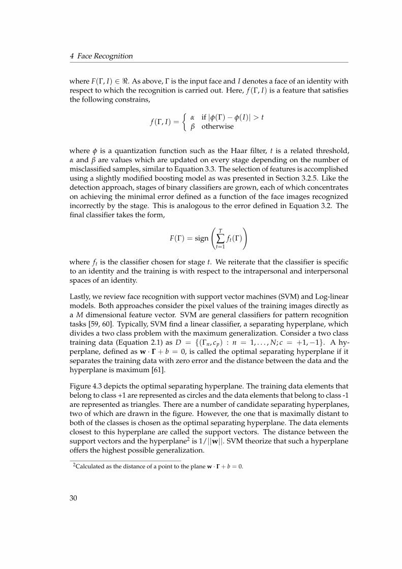
Figure 4.3 depicts the optimal separating hyperplane. The training data elements thatbelong to class +1 are represented as circles and the data elements that belong to class -1are represented as triangles. There are a number of candidate separating hyperplanes,two of which are drawn in the figure. However, the one that is maximally distant toboth of the classes is chosen as the optimal separating hyperplane. The data elementsclosest to this hyperplane are called the support vectors. The distance between thesupport vectors and the hyperplane2 is 1/||w||. SVM theorize that such a hyperplaneoffers the highest possible generalization.
2Calculated as the distance of a point to the plane w · " + b = 0.
30
4.2 Recognition from Intensity Images
support vectors
1||w||
Figure 4.3: A separating hyperplane found by SVM. The dotted lines are candidatehyperplanes. However, the filled line is maximally distant from both thecircles and the triangles. Accordingly the elements closest to the hyperplaneare called support vectors. The distance between a support vector and ahyperplane is equated to 1/||w||.
A support vector machine must satisfy,
cn|(w · !n) + b| ) 1, n = 1, . . . , N
where the margin between the hyperplane and the data (1/||w||) must be maximized.However, due to the possibility that there is no hyperplane that perfectly separates thetwo class problem, soft margins are allowed with a penalty function C. Support vectormachines are modeled as the following optimization problem [62, 63],
minw,b,!
=12
wTw + CN
#n=1
)n (4.4)
subject to,cn(wT((!n) + b) ) 1' )n,
)n ) 0
where ) is the error on classification. It should be noted that C is the penalty and isunrelated to c, the class label. To allow for non-linear classification, kernel functions
31

4 Face Recognition
are introduced. For instance, the radial basis function on our task is defined as
K(wi, !j) = exp('*||wi ' !j||2),
where * should be greater than 0. We arrive at suitable values for C and * using cross-validation. Support vector machines are used for face recognition using the one-on-oneapproach for multi-class data. A total of P(P' 1)/2 SVM are built between every pos-sible pair of identities. The image is classified with every SVM, the returned identity iscollected for each SVM and a simple voting procedure awards the final identity. For in-stance, if there are three identities {0, 1, 2}, there are three SVM to build: $0|$1, $0|$2and $1|$2. If the SVM results with respect to an input face ! are {0, 0, 1} respectively,the identity awarded is 0.
Log-linear models are also general pattern recognition classifiers and calculate theBayesian maximum a posteriori probability of an input face ! for every identity. Thescores returned are ranked to return the final identity. The probability of ! belongingto an identity $m is calculated as
p(m|!) =exp[$ + +m f (!)]
P
#m=1
exp[$ + +m f (!)], (4.5)
where f is a feature of the input face and the $ accounts for bias in the model. Thefeature, as we mentioned above, are the pixel intensities as an M dimensional vector.The sum in the denominator in Equation 4.5 is referred to as the normalization con-stant. The +m is calculated from the corresponding training data using the generalizediterative scaling algorithm [64]. The generalized iterative scaling algorithm convergeson the distribution of pixel intensities for each class. The score of the input face withrespect to every identity is calculated and ranked to return that with the highest valueas the final identity.
4.3 Databases
We present a brief introduction to a few important training face databases. We alsopresent important test collections to measure the detection accuracy. Subsequently,we introduce the FERET evaluation, which is an important evaluation benchmark forrecognition algorithms.
32
4.3 Databases
4.3.1 Training Collections
Most training data collections are common to both detection and recognition. Theindividual approach of detection, feature extraction or recognition may have additionalconstraints on the format of the training images. For instance, an approach that reliesheavily on the eye feature localization may expect training images where eye contoursare known. For the sake of brevity, we do not present any annotations that might beavailable.
• Face Database, Universidad Politecnica de Valencia consists of 40000 face im-ages [65] with minor illumination variations. The faces are perfectly croppedfrom the forehead to the lower jaw.
• MIT Database consists of the faces of 16 people. There are 27 pictures availableper person taken under different conditions of illumination, scale and pose [66].
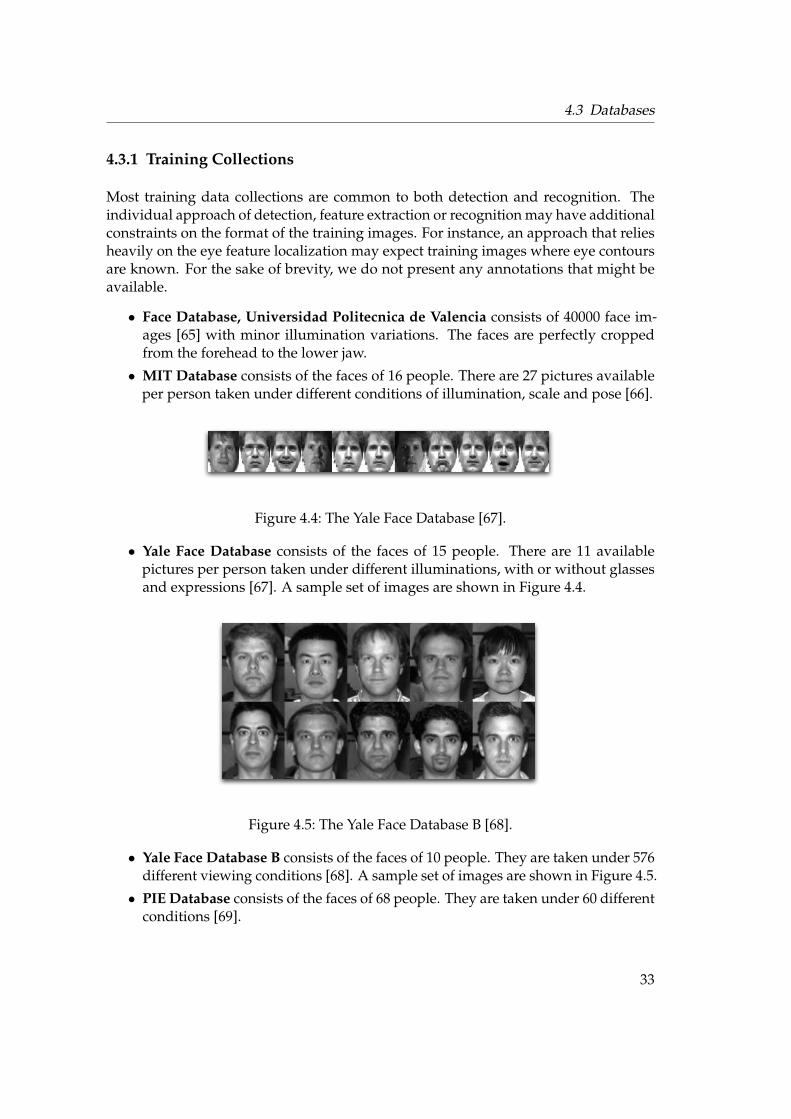
Figure 4.4: The Yale Face Database [67].
• Yale Face Database consists of the faces of 15 people. There are 11 availablepictures per person taken under different illuminations, with or without glassesand expressions [67]. A sample set of images are shown in Figure 4.4.
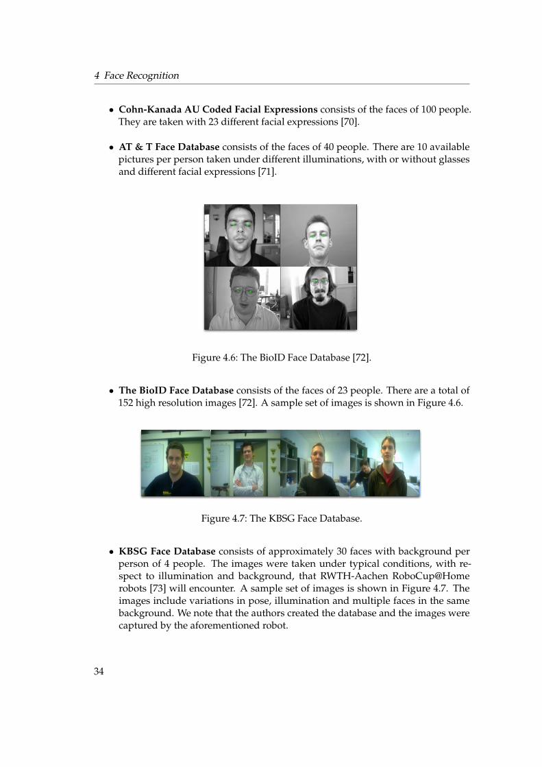
Figure 4.5: The Yale Face Database B [68].
• Yale Face Database B consists of the faces of 10 people. They are taken under 576different viewing conditions [68]. A sample set of images are shown in Figure 4.5.
• PIE Database consists of the faces of 68 people. They are taken under 60 differentconditions [69].
33
4 Face Recognition
• Cohn-Kanada AU Coded Facial Expressions consists of the faces of 100 people.They are taken with 23 different facial expressions [70].
• AT & T Face Database consists of the faces of 40 people. There are 10 availablepictures per person taken under different illuminations, with or without glassesand different facial expressions [71].
Figure 4.6: The BioID Face Database [72].
• The BioID Face Database consists of the faces of 23 people. There are a total of152 high resolution images [72]. A sample set of images is shown in Figure 4.6.
Figure 4.7: The KBSG Face Database.
• KBSG Face Database consists of approximately 30 faces with background perperson of 4 people. The images were taken under typical conditions, with re-spect to illumination and background, that RWTH-Aachen RoboCup@Homerobots [73] will encounter. A sample set of images is shown in Figure 4.7. Theimages include variations in pose, illumination and multiple faces in the samebackground. We note that the authors created the database and the images werecaptured by the aforementioned robot.
34

4.3 Databases
4.3.2 Test Data Collection
One of the earliest test collections was by Sung and Poggio [42]. The second collec-tion created by Sung and Poggio consisted of 23 low resolution images with complexbackgrounds and faces occupying relatively smaller areas.
Figure 4.8: A few samples from the CMU test data collection. In addition to frontal poseface images, the collection includes rotated faces, complex backgrounds andmultiple faces, in close proximity of each other.
Images of comparable complexity are also offered as part of the CMU test collection [74].The CMU collection has 130 images with 507 frontal face images. The collection alsohas a few rotated faces which makes the detection task more challenging. Anothertest collection, the CMU Profile Face Images [75] contain 50 images with 223 face
35
4 Face Recognition
profiles (most at an angle) also in complex backgrounds. The above collections can beconsidered to be real-life scenarios as they created from an variety of sources includingmusic album covers, family and celebrity pictures, stills from TV shows etc. Figure 4.8shows a few samples.
4.3.3 FERET Protocol
The FERET protocol is a set of evaluations and it remains to be the most important datacollection for face recognition. The FERET protocol is intended to be a framework thatpresents a real-world setting for recognition systems [76, 26].
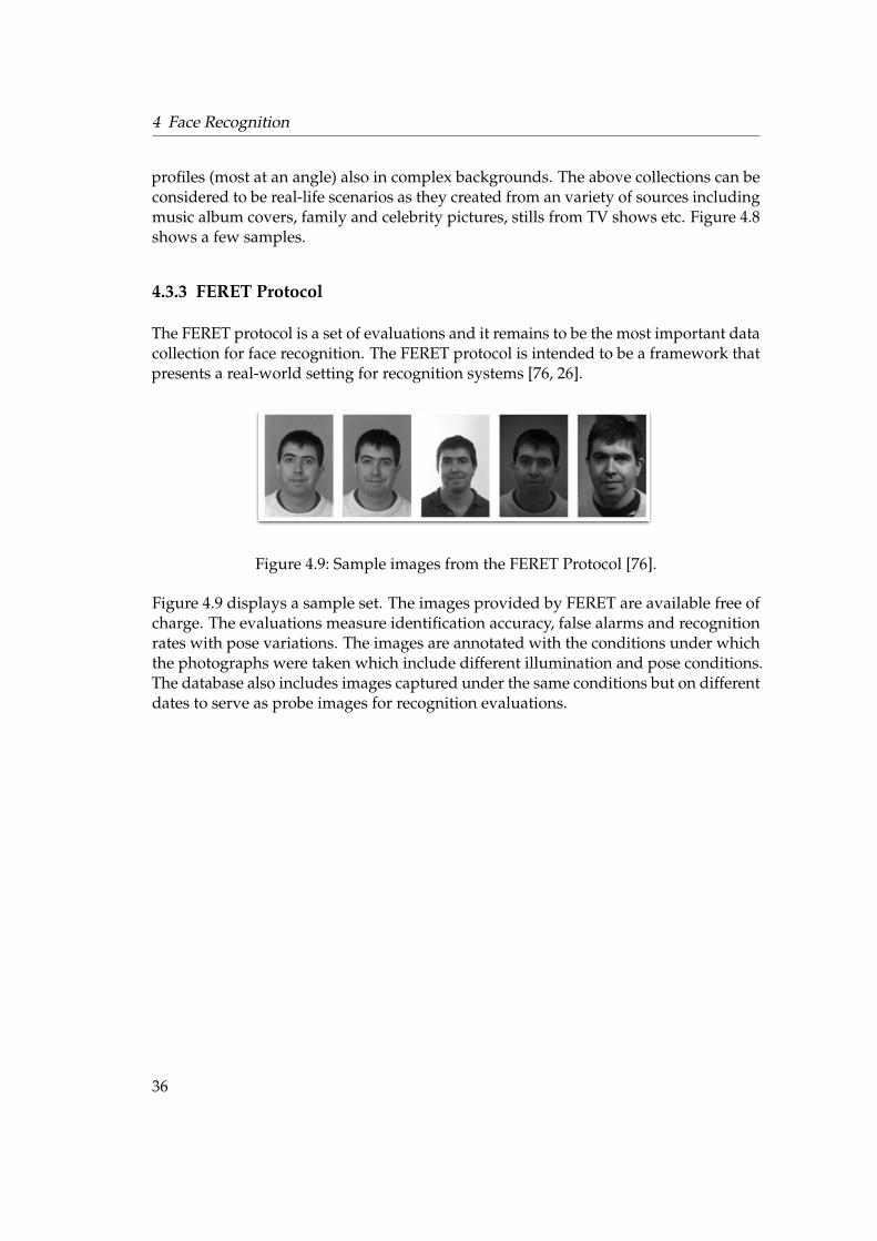
Figure 4.9: Sample images from the FERET Protocol [76].
Figure 4.9 displays a sample set. The images provided by FERET are available free ofcharge. The evaluations measure identification accuracy, false alarms and recognitionrates with pose variations. The images are annotated with the conditions under whichthe photographs were taken which include different illumination and pose conditions.The database also includes images captured under the same conditions but on differentdates to serve as probe images for recognition evaluations.
36

5 FRAMEWORK
In this chapter we detail our framework. Our proposal was towards a unified frame-work for face detection, recognition and learning of human faces with random forests.
In Section 5.1, we present the theoretical foundations of random forests. In Section 5.2,we review training data requirements of a learning framework, especially that of a faceprocessing system. In Section 5.4, we describe the procedure to build random treesfor our framework. We present face detection with random forests in Section 5.5. Wepresent our arbitration techniques in Section 5.6. We finally present face recognitionand face learning with random forests in Section 5.7 and Section 5.8.
5.1 Theoretical Foundations of Random Forests
In Section 1.2, we mentioned that random forests have distinct advantages over clas-sical decision trees. In this section, we clarify our claim and present the theoreticalfoundations of random forests.
5.1.1 Decision Trees
Classic Decision Trees [18], such as C4.5 and its earlier cousin ID3, recursively growtrees top down by maximizing the information gain at the nodes [77, 78] with respectto the training data. Training data is typically of the form,
D =!"
!n, cp#
: n = 1, . . . , N; p = 1, . . . , P$
(5.1)
where, !N1 are the data elements and cP
1 are the corresponding class labels. Further, thedata elements, !n, are M dimensional i.e. they have M attributes. C4.5 (and ID3) searchfor the attribute that offers maximal information gain at the parent node. This searchis geometrically a hyperplane that best divides the training data and characterized byany of the M attributes taking on a specific value. If we model an attribute to be adiscrete random variable, X, the information gain of this hyperplane is given with theShannon Entropy as
37

5 Framework
H(X) = 'P
#m=1
p(xm) · log p(xm), (5.2)
where p(xm) is the probability of the division with respect to class m. Thus, the algo-rithm finds the hyperplane, parallel to an axis in the M dimension, with the lowestH and divides the training data into two groups. The groups serve as the trainingdata to the child nodes. The procedure recurs at the child node. Algorithm 1 brieflysummarizes our review.
Algorithm 1 A decision treeRequire: training data collection, D
1: for all attributes do2: calculate information gain with this attribute as the hyperplane3: end for
4: choose attribute with highest information gain5: create a decision node and divide the training collection6: recur procedure till nodes encounters no more examples
As Russell and Norvig [18, 21] discuss, a serious limitation of decision trees is that ofoverfitting. Overfitting is the condition of a grown decision tree that is meticulouslyconsistent with the training data and yet not learnt "useful" information. The tree has,in this case, maximized information gain on non-critical attributes due to the highdimensionality of the training data and the attributes are too general to be of any use.The shortcoming is critical to our work since image data is very high dimensional.An unseen example with a few variations will be incorrectly classified. The standardtechnique to deal with overfitting is with decision tree pruning. Decision tree pruningseeks to reduce the redundancy of the decision nodes. It traverses the tree to find nodeswith zero information gain and shortens the tree by removing such nodes. However,decision tree pruning equivalently reduces the classification accuracy of the decisiontree.
5.1.2 Random Forests
It remains that decision tree classifiers are popular due to their intuitive appeal andeasy training procedures. Pruning procedures, as described above, might increasegeneralization accuracy but simultaneously reduce the classification accuracy on thetraining samples. There is no classical decision tree approach to increase both classifica-tion and generalization accuracy [21]. Tin Ho [21] discusses that this limitation lies notin trees themselves and introduces oblique trees. Oblique trees do not seek hyperplanesparallel to any axis, as was with classical decision trees. Instead, the two farthest data
38

5.1 Theoretical Foundations of Random Forests
samples are estimated with Euclidian distance measures and connected to each other.A hyperplane perpendicular to the projection of this connection serves as the divisioncriteria.
While such hyperplanes avoid redundant attributes, the more important generalizationaccuracy does not necessarily improve. To address generalization we need a collectionof classifiers, each of which should be trained independently [22, 21, 1].
Subsequently, Tin Ho introduces a random forest. "Random forests are a combination oftree predictors such that each tree depends on the values of a random vector sampledindependently and with the same distribution for all the trees in the forest" [1]. Arandom tree is built by choosing components from random subspaces [21, 22]. Eachrandom tree is trained on the entire training data. However, the trees randomize featureselection and decision criteria. Since we assume the training data to be M dimensional,there are 2M random subspaces to choose from. Ho further discusses that very highclassifier accuracies can be achieved with an increasing number of trees.
The underlying nature of random forests is that of building classifiers independently.This makes their construction inherently parallel, allowing us the flexibility to exploitparallel computing architectures. It is, as a result, referred to as a parallel learning algo-rithm [22].
We note that classifiers from random subspaces are not the only complex classifierspossible. Groups of classifiers built with cross-validation, bagging and boosting are allrelevant multiple classifiers. Cross-validation is another approach to address overfit-ting [18]. Here, the training data is divided into sets of two collections with the learningframework training on one and an intermediate test procedure measures generalizationerrors on the other. Further, while bagging [19, 78] allows training of different classifiersusing overlapping and randomized subsets of the training data, boosting [21, 79, 22]builds stages of classifiers with each stage concentrating on the samples misclassifiedwith the previous stage. We have previously, in Section 3.2.5 and Section 4.2, presentedapproaches that use boosting to detect faces and recognize faces respectively.
We summarize and note that random forests create a large number of independentlytrained classifiers by the random sampling of rectangular features. Breiman [1] presentsa discussion on the convergence of random forests and why overfitting will not occur.While an exhaustive theoretical review of this work is beyond the scope of this thesis, itis interesting to note that the generalization error converges to a limit as the number oftrees in the forest increases. In the next section, we review two important parametersthat directly influence the generalization error of a random forest.
39

5 Framework
5.1.3 Generalization Error
In this section, we present a brief summary of the mathematical treatment on randomforests by Breiman [1]. The principal objective is to obtain a relation for the generaliza-tion error of random forests. Breiman derives an equation for the generalization errorin terms of the strength of each random tree and the correlation between them.
Any application of random forests is characterized by a random vector , that samplesthe training data. For instance, in the approach taken by Marée et al. [5, 6, 9, 10], ,represents a random rectangle. Amit et al. [80] build classifiers with a random selectionof binary geometric features. The ,, in this case, is an integer l such that l ( {1, . . . , L}where L is the number of geometric features considered. A random tree is a classifierdefined as h(x, ,k) where k ( {1, . . . , K} is the index of the tree in the forest and x is theinput vector. The value y(k) = h(x, ,k) is the class label of x as determined by randomtree k. We note that the space of input vectors is X and the space of class labels is Y. Therandom forest, a collection of classifiers, is correspondingly defined as,
{h(x, ,k); k = 1, . . . , K}. (5.3)
It is important to note that each ,k represents an independent sampling and the sam-pling is from the same distribution. This implies that the random features chosen forour approach are taken from the same training data for each tree and the features areindependently chosen from each other. The random trees defined cast a vote each andthe votes are combined to return the class label y.
Let us now consider any general classifier hk(x). For an ensemble of the classifiers{h1(x), h2(x), . . . , hk(x)}, Breiman introduces the margin function as:
mg(X, Y) = akI(hk(X) = Y)'maxj +=Y (akI(hk(X = j)) (5.4)
where a represents the average and I the indicator function. The indicator functionreturns 1 if the relation specified holds and 0 if not. For instance, I(hk(X) = Y) returns 1in case a classifier hk(X) returns the correct class of the input vector. Thus, Equation 5.4simply tells us by how much, on an average, does the classifier return the precise classlabel compared to the most common incorrect class label.
The generalization error is modeled using the margin function as,
PE" = PX,Y (mg(X, Y) < 0) (5.5)
which is the probability over the space of the input vectors and class labels.
Breiman substitutes the definitions in the random forest framework. The margin func-tion, now termed mr, is defined as,
mr(X, Y) = P, (h(X, ,) = Y)'maxj +=Y (P, (h(X, ,) = j)) (5.6)
40

5.1 Theoretical Foundations of Random Forests
where , is the random sampling of rectangular features as defined above. It is clearthat mr is closely related to the generalization error. Breiman thus defines the strengthof the ensemble (Equation 5.3) as,
s = EX,Y (mr(X, Y)) . (5.7)
where E is the mathematical expectation. The mean correlation - between the classifiersis derived as a function of E, the standard deviation and the random vector ,k. Breimanobtains the upper bound on the generalization error as:
PE" , -(1' s2)
s2 . (5.8)
The equation above gives us a clear indication that the generalization error is influ-enced by two factors, the correlation between the random trees and their individualstrengths. Further, the mean correlation is related to the independence of ,k and thus,the generalization error is directly proportional to the randomization and the indepen-dence of ,k. Breiman further derives that as the number of random trees becomes large(tends to infinity), the generalization error converges to a limit. Although in practice,we do not intend to grow an infinite number of random trees, growing as few as 10trees presents very competitive results [1, 7, 21, 22, 11, 9, 6, 10, 12, 41].
5.1.4 Conclusion
We summarize, briefly, the benefits of growing random forests with a random samplingof features. The advantages are [16, 1]:
1. Straightforward Learning. The random sampling of features does not imposeany explicit template or model. A generic algorithm learns characteristics directlyfrom the training data.
2. Local Representation. The randomly sampled features directly analyze the im-age region without explicitly extracting geometric primitives such as edges.
3. Classification with Occlusion. As discussed in Chapter 2, approaches that userandom forests are able to classify and detect partially occluded objects since notall the sampled regions need to be accurately classified. The voting procedureallows for a few sampled subwindows to be falsely classified.
4. Parallelization. Equation 5.8 emphasizes the independent training of randomtrees and as a result, parallel architectures can be used to grow each tree of arandom forest.
5. Fast Training Time. Breiman discusses the fast training time of random forests.As random features are selected, no computational time is spent on searchingfor the most discriminative attribute. Thus, at each node only a single decisioncriterion is instantiated.
41

5 Framework
6. Comparable Accuracy. Breiman also discusses that random forests perform fa-vorably in comparison to adaptive boosting based approaches. This is attributedto the fact that multiple classifiers are built, each with a decent classificationaccuracy.
7. Low Generalization Error. As we discussed in Section 5.1.3, the generalizationerror tends to a limit as the number of random trees grown increases.
8. Integrated approach for tasks. Creating a collection of learned features andquerying them is a part of the same framework. This factor is influential in pre-senting a unified approach to detection and recognition as we discuss in Chap-ter 5.
5.2 Training Data Requirements
A learning framework is characterized by two entities: a learning algorithm and train-ing data. The learning framework describes a procedure for extracting meaningfulinformation from the training data. The training data, correspondingly, must be repre-sentative enough for all the classes. To increase robustness and the capability to workin real life scenarios, annotated training data with real life backgrounds are included.Thus, the algorithm is trained to classify, detect or recognize objects in spite of thecomplex backgrounds encountered when deployed.
Annotations are dependent on the problem definition. Typically, prospective trainingdata for face detection are images with faces that cover the entire image as in case ofFigure 4.4 or Figure 4.5. However, faces in bigger backgrounds as in case of Figure 4.6or faces in complex backgrounds as in Figure 4.8 can also serve as training data. Anno-tations, here, detail the exact location and extent of every face in the images. Further,training images for face recognition systems require that the faces are labeled with theidentity of the person.
We note that for face detection or recognition systems that principally work with facialfeatures such as eyes and noses, an additional requirement is imposed on the trainingdata. Training images here are annotated with the position and extent of relevantfeatures.
As described in Equation 5.1, the training data is usually of the form
D =!"
!n, cp#
: n = 1, . . . , N; p = 1, . . . , P$
,
where !N1 represent the N training images, cP
1 represent the P class labels. The image!n is considered to be M dimensional. We further denote each pixel value with !n(x, y)which denotes the pixel intensity at the (x, y) coordinate of !n.
42

5.3 Learning Framework
Face detection is a two class problem: to identify if a sample is a face or not a face. Thetraining images for the face detection, accordingly, are divided into two: face imagesand background images. Any image that does not contain faces can effectively consti-tute the background images collection. This may include domestic objects such as bikesand cars, animals, and any typical background such as walls and furniture. Typically,the size of the non-face collection exceeds the face collection in the training data forface detection. This is attributed to the fact that a larger group of entities constituteas non-faces. As low false positives is usually desired, better performance is achievedwith a more comprehensive non-face collection. Face recognition, on the other hand, ismodeled as a P class problem with one class assigned to each of the P identities. Thetraining images for face recognition are, accordingly, divided into P collections.
5.3 Learning Framework
In this section we discuss our learning framework. The learning framework detailsthe randomization of decision criteria, the filter and features used and an efficientrepresentation for computation that we borrow from Viola and Jones [30].
5.3.1 Decision Criteria
A randomized decision criterion consists of a randomly sampled rectangle, i.e. of randomdimensions and at a random location, and an accompanying randomly chosen threshold.We present an overview of our learning framework and the decision criterion.
Our learning framework is comprised of growing random trees from the labeled train-ing data. Random trees are recursively built in a top-down manner. At each node t, thetraining images at the node "t are split into two groups, "l and "r. The groups corre-spond to the training images at the left and right branches of the node respectively [12].The split is the result of a decision criterion acting on quantized random patches.
The split is disjoint with "t = "l - "r and "l . "r = Ø. The nodes tl and tr correspondto the left and right nodes of t. The image collections "l and "r are now the trainingdata at tl and tr respectively and the procedure is repeated. The tree is grown until theimage collection at the node consists of images from only one class. For instance, in thecase of the two class face detection problem, the training images are recursively splituntil the node has either only faces or only non-faces. An alternate growth stoppingcriterion are the number of nodes that the tree is allowed to grow. This criteria is borneout of the need to constrain memory requirements when it is known in advance orexperimentally estimated that a specific number is sufficient for a desired accuracy.
43

5 Framework
The framework randomly samples the training images. Random sampling signifies thata patch whose position and extent is completely random (but within the dimensions ofthe training images) is considered. Needless to say, the position and extent is the samein all the training images at a particular node. However, if the training images are notall of the same dimensions, either all of them are rescaled to K! L (where K " L = M)or the position and extent is chosen relatively in every image with respect to an Mdimensional image. The patch selected is represented as {xt, yt, ht, wt} where xt is thex-coordinate of the top left corner of the patch, yt is the y-coordinate of the top leftcorner of the patch, ht is the height and wt is the width of the patch.
The framework selects a random threshold. The threshold is also randomly chosen inthe range of minimal and maximal values that a quantized patch can take. Mossmann etal. [12] and Marée et al. [9] refer to random trees with thresholds also chosen randomlyas extremely random trees. We however exclude the qualifier for the sake of brevity.We denote the threshold for the node t as ,t. We summarize the above as a tuple,Tt = {xt, yt, ht, wt, "l , "r, ,t} and refer to it as a test. Here, "l and "r are not specific toa test, but since we generally instantiate one test per node t, we consider all of themtogether.
We note that the threshold can also be a range as opposed to a single number. Insteadof probing if the quantized scalar value exceeds ,t, we could assert if the value lies in(,t1, ,t2). However, this is a minor detail and as the thresholds are randomly chosen,the number of thresholds is not important.
5.3.2 Features
The patches sampled thus are quantized as a scalar quantity or a lower dimensionalvector quantity. The purpose of quantization is to extract meaningful information andexecute operations, such as a test Tt defined above. A filter is applied on the patch andthe output of the filter is the feature. Earlier, in Section 4.1, we discussed Haar filtersand Gabor filters. A Haar or a Gabor filter applied on a region of the image gives usthe Haar feature or the Gabor feature of that region.
The desired properties of any feature is that it contains both generative and discrimina-tive information with respect to the training data. Generative information are proper-ties that can reconstruct the image, such as the M& dimensional vector in PCA. Discrim-inative information between two classes are properties that highlight the differencesbetween the classes. Haar features are generative and discriminative [54]. In the adap-tive boosting based face detector [30], Haar filters successfully learnt discriminatoryfeatures between the face and non-face class. Tao et al. [81] discuss that bases from abinary subspace can be used as generative components of images. Haar features canbe considered to be binary bases [54, 30] and hence contain generative information.
44
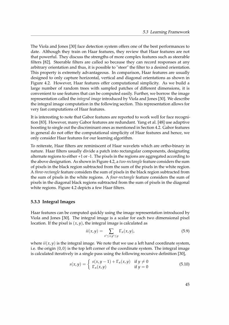
5.3 Learning Framework
The Viola and Jones [30] face detection system offers one of the best performances todate. Although they train on Haar features, they review that Haar features are notthat powerful. They discuss the strengths of more complex features such as steerablefilters [82]. Steerable filters are called so because they can record responses at anyarbitrary orientation and thus, it is possible to "steer" the filter to a desired orientation.This property is extremely advantageous. In comparison, Haar features are usuallydesigned to only capture horizontal, vertical and diagonal orientations as shown inFigure 4.2. However, Haar features offer computational simplicity. As we build alarge number of random trees with sampled patches of different dimensions, it isconvenient to use features that can be computed easily. Further, we borrow the imagerepresentation called the integral image introduced by Viola and Jones [30]. We describethe integral image computation in the following section. This representation allows forvery fast computations of Haar features.
It is interesting to note that Gabor features are reported to work well for face recogni-tion [83]. However, many Gabor features are redundant. Yang et al. [48] use adaptiveboosting to single out the discriminant ones as mentioned in Section 4.2. Gabor featuresin general do not offer the computational simplicity of Haar features and hence, weonly consider Haar features for our learning algorithm.
To reiterate, Haar filters are reminiscent of Haar wavelets which are ortho-binary innature. Haar filters usually divide a patch into rectangular components, designatingalternate regions to either +1 or -1. The pixels in the regions are aggregated according tothe above designation. As shown in Figure 4.2, a two-rectangle feature considers the sumof pixels in the black region subtracted from the sum of the pixels in the white region.A three-rectangle feature considers the sum of pixels in the black region subtracted fromthe sum of pixels in the white regions. A four-rectangle feature considers the sum ofpixels in the diagonal black regions subtracted from the sum of pixels in the diagonalwhite regions. Figure 4.2 depicts a few Haar filters.
5.3.3 Integral Images
Haar features can be computed quickly using the image representation introduced byViola and Jones [30]. The integral image is a scalar for each two dimensional pixellocation. If the pixel is (x, y), the integral image is calculated as
ii(x, y) = #x&,x,y&,y
!n(x, y), (5.9)
where ii(x, y) is the integral image. We note that we use a left hand coordinate system,i.e. the origin (0, 0) is the top left corner of the coordinate system. The integral imageis calculated iteratively in a single pass using the following recursive definition [30],
s(x, y) =%
s(x, y' 1) + !n(x, y) if y += 0!n(x, y) if y = 0 (5.10)
45

5 Framework
1 2
3 8
A B
C D
56
7
Figure 5.1: The sum of pixels in the rectangle A is the integral image at location 1. Thesum of pixels in the rectangle B is 2' 1. The sum of pixels of A + C is theintegral image at 3. The sum of pixels in D is 8 + 6' 7' 5.
ii(x, y) =%
ii(x' 1, y) + s(x, y) if x += 0s(x, y) if x = 0 (5.11)
where s is the sum of pixels.
In Figure 5.1, a typical computation is illustrated. The figure denotes an integral imagerepresentation. As we see in the figure, the sum of pixels for an arbitrary region can becalculated with only four array references. This integral image calculation needs to bedone only once for an image, irrespective if it is used for training or as a test image.
5.4 Growing Trees
As discussed earlier, the tree is recursively grown with "t at node t using the testTt = {xt, yt, ht, wt, "l , "r, ,t}. Before we review how the features are chosen, we considerthe simple two-rectangle feature as shown in Figure 4.2. Here, (xt, yt) represents thetop left corner of the sampled patch. Figure 5.2 lists the remaining coordinates.
The sum of pixels in the black region of the image patch is obtained by evaluating thevalues in the integral image as,
s(black) = (xt + wt, yt + ht) + (xt +wt
2, yt)' (xt +
wt
2, yt + ht)' (xt +
wt
2, yt).
46
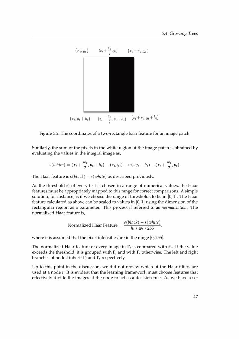
5.4 Growing Trees
(xt, yt) (xt +wt
2, yt) (xt + wt, yt)
(xt, yt + ht) (xt +wt
2, yt + ht) (xt + wt, yt + ht)
Figure 5.2: The coordinates of a two-rectangle haar feature for an image patch.
Similarly, the sum of the pixels in the white region of the image patch is obtained byevaluating the values in the integral image as,
s(white) = (xt +wt
2, yt + ht) + (xt, yt)' (xt, yt + ht)' (xt +
wt
2, yt).
The Haar feature is s(black)' s(white) as described previously.
As the threshold ,t of every test is chosen in a range of numerical values, the Haarfeatures must be appropriately mapped to this range for correct comparisons. A simplesolution, for instance, is if we choose the range of thresholds to lie in [0, 1]. The Haarfeature calculated as above can be scaled to values in [0, 1] using the dimension of therectangular region as a parameter. This process if referred to as normalization. Thenormalized Haar feature is,
Normalized Haar Feature =s(black)' s(white)
ht " wt " 255,
where it is assumed that the pixel intensities are in the range [0, 255].
The normalized Haar feature of every image in "t is compared with ,t. If the valueexceeds the threshold, it is grouped with "l and with "r otherwise. The left and rightbranches of node t inherit "l and "r respectively.
Up to this point in the discussion, we did not review which of the Haar filters areused at a node t. It is evident that the learning framework must choose features thateffectively divide the images at the node to act as a decision tree. As we have a set
47

5 Framework
of Haar filters, we use the Shannon Entropy to select one. The entropy of a split iscalculated as,
H = '#P
p · log p, (5.12)
where H is the entropy, p is the probability of a class with respect to the division and iscalculated for every class in {1, . . . , p}. In the case of the face detection problem,
p f =number of faces in "lnumber of faces in "t
pn f =number of non-faces in "lnumber of non-faces in "t
where "l and "t are as above, p f is the probability of the face class with respect to thedivision and pn f is the probability of the non-face class with respect to the division. Foreach normalized Haar feature the entropy is calculated with respect to ,t. We choosethe Haar feature with the smallest value for H. A Haar filter that proves most effectiveat a node is highly dependent on the training images at the node. Thus, there is usuallyno single Haar filter that is effective for every node of the random tree. We note that wecan estimate probabilities with respect to "r with an completely identical treatment.
Figure 5.3 illustrates the growth of a random tree. At the node t, there are four images,two faces and two background images. A two-rectangle Haar filter is chosen (corre-sponds to the region around the eye in the face images). The Haar filter is characterizedby the sum of the pixels in the left component subtracted from the sum of the pixelsin the right component. As the pixel values in the left and right eye is very similar,the Haar feature leads to a very small value (close to zero). Similarly, the first back-ground image also has a homogenous appearance in the region. In comparison, thesecond background image has considerable disparity. On comparing the feature withthreshold ,t, the first three images are separated. The last image is placed in a leaf nodeand does not undergo further growth. Another two-rectangle Haar filter is randomlysampled at node t + 1. However, the feature does not prove discriminatory enough todivide the images at the bin. A two-rectangle filter at node t + 2 and the threshold ,t+2separate the faces from the background image. As both children of node t + 2 containimages from only a single class, they remain as leaf nodes and the growth is stopped.
In the figure above, the growth is accomplished in 4 levels of the tree. In the actualexecution path, this may be different. Haar features that separate image classes maybe sampled after an arbitrary number of levels. Further, the threshold ,t in the figurecorrectly separated similar numerical quantities. In an extremely random tree, thethresholds need not account for a separation even in the case of quantized features thatare linearly separable. We can thus expect arbitrary divisions at arbitrary depths. Asdiscussed before, the randomization affords us high generalization accuracy.
However, at the cost of generalization accuracy, the tree might be grown to large depthson redundant and non-discriminatory random patches. To circumvent this problem,
48
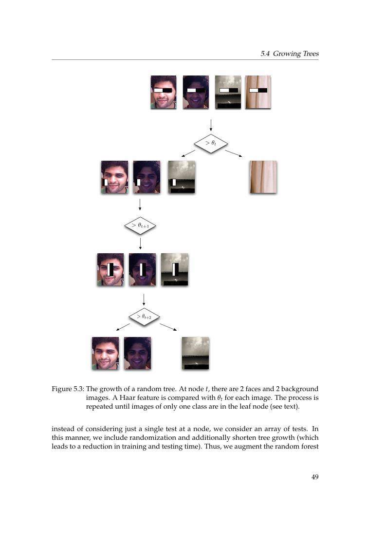
5.4 Growing Trees
> !t
> !t+1
> !t+2
Figure 5.3: The growth of a random tree. At node t, there are 2 faces and 2 backgroundimages. A Haar feature is compared with ,t for each image. The process isrepeated until images of only one class are in the leaf node (see text).
instead of considering just a single test at a node, we consider an array of tests. Inthis manner, we include randomization and additionally shorten tree growth (whichleads to a reduction in training and testing time). Thus, we augment the random forest
49
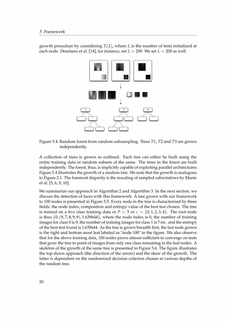
5 Framework
growth procedure by considering Tt[L], where L is the number of tests initialized ateach node. Deselaers et al. [14], for instance, set L = 200. We set L = 200 as well.
T1 T2 T3
Figure 5.4: Random forest from random subsampling. Trees T1, T2 and T3 are grownindependently.
A collection of trees is grown as outlined. Each tree can either be built using theentire training data or random subsets of the same. The trees in the forest are builtindependently. The forest, thus, is implicitly capable of exploiting parallel architectures.Figure 5.4 illustrates the growth of a random tree. We note that the growth is analogousto Figure 2.1. The foremost disparity is the rescaling of sampled subwindows by Maréeet al. [5, 6, 9, 10].
We summarize our approach in Algorithm 2 and Algorithm 3. In the next section, wediscuss the detection of faces with this framework. A tree grown with our frameworkto 100 nodes is presented in Figure 5.5. Every node in the tree is characterized by threefields: the node index, composition and entropy value of the best test chosen. The treeis trained on a five class training data or P = 5 or c = {0, 1, 2, 3, 4}. The root nodeis thus {0, (9, 7, 8, 9, 9), 1.639644}, where the node index is 0, the number of trainingimages for class 0 is 9, the number of training images for class 1 is 7 etc. and the entropyof the best test found is 1.639644. As the tree is grown breadth first, the last node grownis the right and bottom most leaf labeled as "node 100" in the figure. We also observethat for the above training data, 100 nodes prove almost sufficient to converge on teststhat grow the tree to point of images from only one class remaining in the leaf nodes. Askeleton of the growth of the same tree is presented in Figure 5.6. The figure illustratesthe top-down approach (the direction of the arrow) and the skew of the growth. Thelatter is dependent on the randomized decision criterion chosen at various depths ofthe random tree.
50
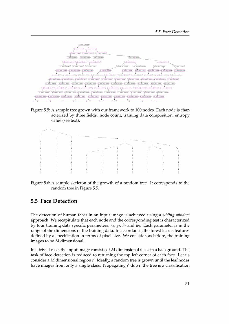
5.5 Face Detection
0 9,7,8,9,9 1.639644
1 7,0,0,0,0 1.584963 2 2,7,8,9,9 1.737926
3 7,0,0,0,0 1.584963 4 0,0,0,6,0 1.672933 5 2,7,8,3,9 1.836175
6 7,0,0,0,0 1.584963 7 0,0,0,6,0 1.672933 8 0,0,5,0,0 1.770951 9 2,7,3,3,9 1.918296
10 7,0,0,0,0 1.584963 11 0,0,0,6,0 1.672933 12 0,0,5,0,0 1.770951 13 1,0,1,3,8 1.716917 14 1,7,2,0,1 1.753434
15 7,0,0,0,0 1.584963 16 0,0,0,6,0 1.672933 17 0,0,5,0,0 1.770951 18 0,0,0,3,8 1.626689 19 1,0,1,0,0 2.235926 20 0,7,2,0,0 1.694988 21 1,0,0,0,1 2.235926
22 7,0,0,0,0 1.584963 23 0,0,0,6,0 1.672933 24 0,0,5,0,0 1.770951 25 0,0,0,1,8 1.554049 26 0,0,0,2,0 2.128085 27 1,0,1,0,0 2.235926 28 0,7,0,0,0 1.584963 29 0,0,2,0,0 2.128085 30 1,0,0,0,1 2.235926
31 7,0,0,0,0 1.584963 32 0,0,0,6,0 1.672933 33 0,0,5,0,0 1.770951 34 0,0,0,0,8 1.505876 35 0,0,0,1,0 2.251629 36 0,0,0,2,0 2.128085 37 1,0,1,0,0 2.235926 38 0,7,0,0,0 1.584963 39 0,0,2,0,0 2.128085 40 1,0,0,0,1 2.235926
41 7,0,0,0,0 1.584963 42 0,0,0,6,0 1.672933 43 0,0,5,0,0 1.770951 44 0,0,0,0,8 1.505876 45 0,0,0,1,0 2.251629 46 0,0,0,2,0 2.128085 47 1,0,1,0,0 2.235926 48 0,7,0,0,0 1.584963 49 0,0,2,0,0 2.128085 50 1,0,0,0,1 2.235926
51 7,0,0,0,0 1.584963 52 0,0,0,6,0 1.672933 53 0,0,5,0,0 1.770951 54 0,0,0,0,8 1.505876 55 0,0,0,1,0 2.251629 56 0,0,0,2,0 2.128085 57 1,0,1,0,0 2.235926 58 0,7,0,0,0 1.584963 59 0,0,2,0,0 2.128085 60 1,0,0,0,1 2.235926
61 7,0,0,0,0 1.584963 62 0,0,0,6,0 1.672933 63 0,0,5,0,0 1.770951 64 0,0,0,0,8 1.505876 65 0,0,0,1,0 2.251629 66 0,0,0,2,0 2.128085 67 1,0,1,0,0 2.235926 68 0,7,0,0,0 1.584963 69 0,0,2,0,0 2.128085 70 1,0,0,0,1 2.235926
71 7,0,0,0,0 1.584963 72 0,0,0,6,0 1.672933 73 0,0,5,0,0 1.770951 74 0,0,0,0,8 1.505876 75 0,0,0,1,0 2.251629 76 0,0,0,2,0 2.128085 77 1,0,1,0,0 2.235926 78 0,7,0,0,0 1.584963 79 0,0,2,0,0 2.128085 80 1,0,0,0,1 2.235926
81 7,0,0,0,0 1.584963 82 0,0,0,6,0 1.672933 83 0,0,5,0,0 1.770951 84 0,0,0,0,8 1.505876 85 0,0,0,1,0 2.251629 86 0,0,0,2,0 2.128085 87 1,0,1,0,0 2.235926 88 0,7,0,0,0 1.584963 89 0,0,2,0,0 2.128085 90 1,0,0,0,1 2.235926
node91 node92 node93 node94 node95 node96 node97 node98 node99 node100
Figure 5.5: A sample tree grown with our framework to 100 nodes. Each node is char-acterized by three fields: node count, training data composition, entropyvalue (see text).
Figure 5.6: A sample skeleton of the growth of a random tree. It corresponds to therandom tree in Figure 5.5.
5.5 Face Detection
The detection of human faces in an input image is achieved using a sliding windowapproach. We recapitulate that each node and the corresponding test is characterizedby four training data specific parameters, xt, yt, ht and wt. Each parameter is in therange of the dimensions of the training data. In accordance, the forest learns featuresdefined by a specification in terms of pixel size. We consider, as before, the trainingimages to be M dimensional.
In a trivial case, the input image consists of M dimensional faces in a background. Thetask of face detection is reduced to returning the top left corner of each face. Let usconsider a M dimensional region i&. Ideally, a random tree is grown until the leaf nodeshave images from only a single class. Propagating i& down the tree is a classification
51

5 Framework
Algorithm 2 Random Tree(!n)Require: Training Images, D = {(!n, cp); n = 1, . . . , N; p = 1, . . . , P}.
1: let the current node be t (start with the root node)2: if !t contains images from only one class OR a stopping condition is reached then3: return t4: else5: choose a test, Tt = {xt, yt, ht, wt, "l , "r, ,t}6: split "t as "l and "r such that "l - "r = "t and "l . "r = Ø7: let tl = Random Tree("l) and tr = Random Tree("r)8: let tl and tr be the left and right nodes of t respectively9: return t
10: end if
Algorithm 3 Choose a TestRequire: |"t| > 0.
1: instantiate Tt[L], such that each test, Tt[l] = {xt, yt, ht, wt, "l , "r, ,t}2: for each Tt[l] do3: for each considered Haar feature do4: for each image in "t do5: calculate feature using integral image6: normalize feature as s(black) - s(white)7:8: if s(black)' s(white) > ,t then9: group the image in "l
10: else11: group the image in "r12: end if13: end for14: calculate the entropy as H = '#
Pp · log p
15: end for16: choose the Haar feature with lowest H17: end for18: choose the test with lowest H19: return Tt[l]
task. At every node, the test at that node extracts the relevant Haar feature and com-pares it with the threshold. As the Haar features are discriminatory, if i& is a face, then itwill be separated from the majority of the non-face images down the tree. If it reachesa leaf node with only face images, i& is nominated as a face.
52

5.5 Face Detection
Propagating a region of an image on a random tree trained on face and backgroundimages returns an estimate of the likelihood that the region is a face. Thus a regionclassified into a leaf node with only face images is nominated as a face. A regionclassified into a leaf node with only background images is nominated as a backgroundimage.
However, a random tree need not be necessarily grown till the leaf nodes are composedof images from only class. Memory or time constraints are influential parameters for thelearning framework. It is to be noted that the depth of tree is directly proportional to thetime taken for classification as each node represents a test and a comparison. Growingextremely deep trees implicitly impacts training and classification time. Further, weeven grow a collection of trees and in accordance, the growth of the tree is limited to aheuristically chosen node count or depth count.
In accordance, if a leaf node includes images from both classes, the likelihood of thenode to be nominated as a face is referred to as the Face Map Threshold (FMP) and isdefined as:
Face Map Threshold =" f
" f + "n f(5.13)
where FMP is the probability of a face in the node, " f is the number of faces in the leafnode and "n f is the number of non-faces in the same. If i& is propagated to such a leafnode, a global criterion asserts if the FMP calculated is high enough to nominate i& aface.
The algorithm to detect faces in an input image is thus to iteratively sample M di-mensional windows starting from the top-left corner until the bottom-right corner andpropagate them on the tree. Using the FMP, we nominate if the subwindow is a face ora non-face. The iterative sampling thus examines #Iw'K
1 #Ih'L1 subwindows, where Iw
and Ih represents the width and height of the input image. Algorithm 4 summarizesour review.
In the algorithm, the iterative offsets for the sampling procedure is 1, i.e. e and g pro-ceed in steps of 1. To reduce computation time, the offsets in the X and Y directioncould be increased from 1 to 2 or more. In accordance, if a window is sampled at (0, 0),then the subsequent window sampled is located at (2, 0). Once all the windows aresampled in the current row, the next window sampled is at (0, 2).
We have, presently, only discussed detection in the input image under the assumptionthat the dimensions of every face in the input image is equal to M. However, in reallife scenarios, the extent of a face can take on arbitrary dimensions. Further, the same
53

5 Framework
Algorithm 4 Sliding Window for DetectionRequire: Trained tree, t and an input image, i& (K! L).
1: for e from 1 to Iw ' K in steps of 1 do2: for g from 1 to Ih ' L in steps of 1 do3: extract window of dimensions M at (e, g)4: propagate window down the trained tree till a leaf is reached
5: calculate" f
" f + "n f
6: if value > global threshold then7: return face found at (e, g)8: end if9: end for
10: end for
input image can include faces of different sizes due to the distance from the camera. Toaccomplish detection in such images, we conduct a multi-resolution analysis. The inputimage is scaled by different factors and the algorithm outlined above is repeated ateach scale. Note that the regions sampled are always M dimensional. The principalmotivation for multi-resolution analysis is the observation that by downscaling andupscaling an input image, a face at some scale will be K! L.
The detection process so far will result in a large number of "nominations" for thesame face as every sampled subwindow a few pixels in the vicinity of a face will benominated. Further, the multi-resolution analysis will increase both the number ofnominations for a face and the extents. A good post-processing step is crucial. Wereview post-processing in depth in Section 5.6.
As a concluding remark, scaling the input image is not the only way to detect faces ofdifferent sizes. The sampled windows and the tests can be scaled instead. However,scaling each test in a depth first traversal of the tree is much less efficient than scalingthe image just once.
5.6 Post Processing
Given the large number of prospective detected faces, arbitration is crucial for inter-pretable and usable results. There are three types of prospective results:
1. detections returned for a scale s by a random tree,
2. detections returned for all scales {1, . . . , S} by a random tree and
3. detections returned for all scales {1, . . . , S} by the random forest.
54

5.6 Post Processing
Our arbitration procedure considers the prospective results by post-processing detec-tions in the same order as listed above. That is, we first arbitrate detections returnedfor a scale and repeat the same for each scale. Subsequently, we arbitrate detectionsacross all possible scales to obtain a set of detections for the tree. Voting proceduresmerge the detections of each tree in the random forest.
A detection d is characterized by a location and the bounding box such that de ={xe, ye, we, he}, where e is the index of the detection and e ( {1, . . . , E}. The boundingboxes from the multi-resolution analysis are downscaled or upscaled proportionatelyso as to be applicable to the original input image. Correspondingly, the scaled detectiond&e is
d&e =%
xe
s,
ye
s,
we
s,
he
s
., (5.14)
where s is the scale factor.
For each scale, we collect the detections as rs = {d&1, d&2, . . .}. If at the scale of 1 threefaces are detected, we have r1 = {d1, d2, d3}. If at the scale of 1.5 two faces are detected,we have r1.5 = {d&1, d&2} where d&1 and d&2 are calculated using Equation 5.14 with s =1.5.
The detections of the random tree are collected as {rs : s ( S}, where S is the set ofscales considered. Combining the detections is a non-trivial task as it is difficult todefine a global heuristic that works with different types of input images [43].
The foremost step to the merging of detections is to define a neighbor range. The neigh-bor range of a detection window de is a geometric region in the vicinity of de such thatall detection windows that overlap with the region are considered neighbors of de. Weenumerate two strategies, also illustrated in Figure 5.7, to identify neighbors:
• Calculate the point of intersection of the diagonals of the bounding box andconsider the point to be a center of a circle of diameter 2R. The value of R caneither be a fixed constant or can be related to the dimensions of the bounding boxconsidered. All detection windows that overlap with the circle are neighbors.
• With respect to de, all detection windows that overlap with the rectangle areneighbors.
Following the enumeration of neighbors, the detection windows are merged. A generaldefinition of merging is a weighted combination of all the neighbors,
dwavg =%
# $ · x# $
, # $ · y# $
, # $ · w# $
, # $ · h# $
.(5.15)
where dwavg is the merged detection window. For instance, if we consider a simpleaverage of neighbors (Nd), we can rewrite Equation 5.15 as
davg =%
# xNd
, # yNd
, # wNd
, # hNd
.,
55

5 Framework
Figure 5.7: The search for neighboring detection windows by considering either alloverlapping detection windows or a circular region. The neighbors arecalculated with respect to the central square.
where davg is the merged window.
The value of $ in Equation 5.15 can be a function of any characteristics of the detectionwindow. For instance, the detection windows are arranged in decreasing FMP valuesand the detections with the lowest FMP values are discarded completely ($ = 0). Theweight can also be a function of the extent of the bounding box. To exemplify, we pickthe biggest bounding rectangle in the neighborhood. Although this method is simple,we show that it performs well on a broader test set in Chapter 6.
The detection windows from all the trees in the random forests are merged subse-quently. We enumerate two strategies to merge,
• A detection window is nominated for the final result if and only if there is a corre-sponding detection window in the neighborhood in a majority of the remainingrandom trees. This is a weaker equivalent of the AND operator and shares simi-larity to simple voting scheme in classification tasks by Breiman [20, 19, 1], Maréeet. al [9, 5, 6, 10] and others discussed in Chapter 2. This heuristic addresses away to decrease the number of false positives as a detection is nominated only ifthe majority of trees, each with an individual generalization, appoint a region asa face.
56

5.7 Face Recognition
• Detection windows are simply collected from all the random trees. They are re-tained as is with the notable exception of removing duplicates. This is equivalentto the OR operator. This heuristic address low detection accuracy. If a face isnot detected on one tree for reasons such as overfitting, then it is probable to bedetected by another random tree.
The final set of windows are returned as the list of detected human faces.
5.7 Face Recognition
As discussed in Chapter 4, the task of recognition is either that of identification or verifica-tion. Identification is the task to match a new face with a stored or trained collection ofidentities and return the identity of this face if it exists. Verification is the task to checkif the identity alleged by the input face is correct. We model identification and verifi-cation as confidence measures based on the calculation of the identity likelihood. Theidentity likelihood is a probabilistic estimate of a face image belonging to an identityand shares similarity to the FMP discussed previously.
Our recognition framework is a classification approach. The detection phase is as-sumed to correctly return the location and extent of every face in the input image. Thefaces are scaled to K! L and propagated on a random tree in the forest1. To recognizethe identity, the random tree is grown further till the leaf bins contain faces from onlya single identity. Equivalent extensions must be carried out for all the random trees inthe forest. As with detection, the identity present in the leaf node is nominated as theidentity of the face.
To address the possibility that a face belongs to an unknown identity, we include anadditional class in the training data. This class contains face images of many strangers.If the input face is propagated to a leaf node with images from this class, then the faceis nominated to be unknown.
However, growing trees to the point where leaf nodes are composed of faces from onlya single identity maybe extremely time consuming. As random regions are sampled, adiscriminative Haar feature to divide face images of $p'1 from the face images of $p ata leaf node may or may not be found quickly. Thus, we may introduce a constraint onthe number of nodes that the tree is grown to. The number is borne out of experimentalset-ups that render sufficient accuracy.
To reiterate the recognition nominations, if a scaled face image reaches a leaf nodecontaining faces only of $p, the input face is nominated that of $p with the highest
1It is necessary to repeat the propagation of subwindows and not use any of the previous propagationresults at this point as various arbitration techniques finalize the location and extent of faces from theresults of detection.
57

5 Framework
confidence. The identity threshold is 1. If a scaled face image reaches a leaf node con-taining face images of more than one identity, then we calculate the identity thresholdfor this leaf as,
identity likelihood =number of faces of the most dominant identity
total number of face images in the bin
where the dominant identity is as estimated with a simple histogram analysis at the leafnode. If the identity threshold thus calculated exceeds a global confidence threshold,then the image is nominated as a face of the dominant identity. Identities returned fromthe entire forest are collected and a majority voting scheme decides the final identityto return.
We note that our recognition framework is in fact a P + 1 class problem. There are Pidentities and the additional unknown identity. A face image can be nominated as theface of an unknown identity if any of the following two conditions are satisfied:
1. The majority of the votes in the forest return the identity as that of $p+1 (strangeridentity).
2. The majority margin is not large. For instance, 4 random trees nominate the faceas $p, 3 trees nominate the face as $p'1 and so on.
In our approach above, we presented growing every random tree further such thatthe leaf nodes divide the face images from different identities. A simplification of thisapproach is to grow another forest using only the face images as a multi-class trainingdata. The random forest grown for face detection is not modified. The advantages ofthe latter approach are:
• controlling the number of nodes grown is simplified,
• propagating a scaled face down the non-leaf nodes of the previously grown ran-dom forests is unnecessary, and
• as the principal idea is to separate faces of different identities, the classificationresults and the identity nomination will be the same.
It is to be noted that the "detection" random forests have already separated face im-ages of different identities along the tree whilst finding discriminative Haar featuresbetween the face and non-face training data. By growing another random forest, we donot cannibalize those divisions. However, given the simplicity of growing a new forestand low training time [1, 21, 22, 9, 6, 10], we limit our discussions to the latter approach.
Identification and verification is straightforward once the identity threshold is calcu-lated. If the threshold exceeds a heuristically chosen limit, the face is identified as oneof P identities or as an unknown identity. If the identified identity matches the allegedidentity, the face is verified.
58
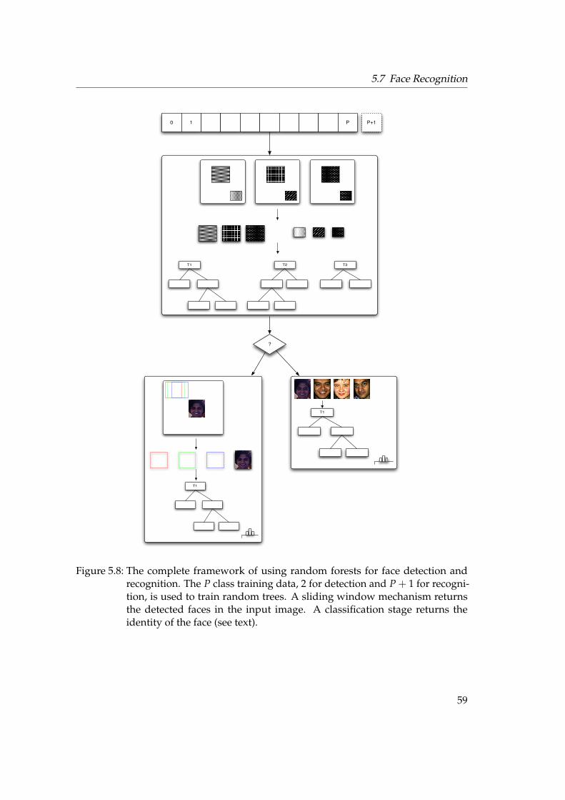
5.7 Face Recognition
T1 T2 T3
0 1 P
?
T1
T1
P+1
Figure 5.8: The complete framework of using random forests for face detection andrecognition. The P class training data, 2 for detection and P + 1 for recogni-tion, is used to train random trees. A sliding window mechanism returnsthe detected faces in the input image. A classification stage returns theidentity of the face (see text).
59

5 Framework
We conclude the recognition framework by considering the four scenarios outlined byTurk and Pentland [39] (discussed in Section 4.2). The scenarios are modified to modelour framework.
1. Regions of the input image do not contain faces and do not share any similar-ity with faces. Our detection framework discards all subwindows that do notcontain faces. Such subwindows are not considered further.
2. Regions of the input image do not contain faces but share a few local visualdescriptors with faces. The random forest iteratively selects discriminatory fea-tures to divide faces and non-faces. If a non-face rectangular region shares afew geometric features with faces, along the depth of tree features are found thatsubsequently separate faces and non-faces.
3. Regions of the input image contain faces but are not similar to any of the iden-tities. In the random forest grown for recognition, face images will be nominatedas belonging to the p + 1 identity.
4. Regions of the input image contain faces and is similar to identity p. Theidentity likelihood will nominate the face as belonging to identity p.
Figure 5.8 describes the overall system. A random forests is grown for detection usingthe two class training data. A random forest is grown for recognition using the P + 1class training data. The sliding window based detection algorithm returns the locationand extent of detected faces in the input image. Each face is now propagated down theforest and an identity is returned based on confidence analyses.
5.8 Face Learning
As part of our motivation, we discussed that if a human face was not recognized asone of the known identities then the robot introduces itself and learns the new identity.This characteristic renders a human-like experience and improves the social interactionbetween humans and robots.
We model face learning also by growing the random trees further. Let us assume themobile robot has introduced itself to a human being ($p&) and images are captured.As it is likely that the images contain faces in backgrounds, we initiate the learningstage with the detection and segmentation of the faces from the backgrounds. Thesegmented faces are the training data for $p& .
Each segmented face is propagated on a tree. At the leaf node, the trees are grown fur-ther till the new identity is separated from the remaining identities at the leaf node. Theimportance of this step is that previously, the random trees for recognition were grownuntil images from only a single identity remained in the leaf nodes or to a heuristically
60

5.9 Parameters
chosen depth. By growing the trees further till the new image is separated respects theclassification accuracy of the forest before the new identity was introduced.
Subsequent to this procedure on all segmented faces, the framework is considered tohave learnt the identity. The recognition framework remains intact and identificationor verification is carried out as before.
We had previously discussed a simplification to growing the random forests for de-tection further to also recognize by building a separate forest only for recognition. Asimilar simplification can be extended here. If the number of identities is not large, therandom forests built for the P + 1 identities can be rebuilt for P + 2 identities2. Thus,we do not need to grow the forest trained on recognition further but simply rebuild thesame with the newly segmented faces as an additional identity.
We conclude our framework with the observation that it is possible to build only a sin-gle random forest for face detection, face recognition and face learning, analogous toDeselaers et al. [14]. Our separation of concerns approach, i.e. independently develop-ing the three tasks, allows for better parameterization and implementation simplicity.
5.9 Parameters
As we deal with several heuristics and decision criteria, we present a review of a fewimportant parameters in this section. We enumerate the same followed by the valuesfound optimal in our experimental setups.
1. Forest Size. This specifies the number of random trees to grow. As we discussedin Section 5.1, increasing the number of trees improves the generalization accu-racy. However, the improved accuracy is at the cost of an increase in the trainingand classification time. For detection, we build either 2 or 3 random trees. Forrecognition, we build between 3 and 20 trees. We note that results on recognitionis faster as we only need to integrate classification results. On the other hand,with detection, a multi-resolution analysis needs to be performed on each of therandom trees.
2. Feature Size. This is the maximum allowed size of sampled subwindows of thetraining data. We train on 24! 24 images and found a parameter tune at 11 to beoptimal. In previous experimental runs on images of other dimensions, such as50! 50, a value of 20 was found optimal. We estimate that values a little less than
2It is assumed that the unknown identity class does not contain any face images of identities that mightbe learnt by the mobile robot.
61

5 Framework
*M · 0.5 would prove optimal. It was additionally found the detection accuracy
lowered when larger limits were allowed.
3. Minimum Feature Size. This is the minimum allowed size of sampled subwin-dows. Preventing instantiation of tests that sampled windows of 1! 1 pixels and2! 2 pixels improved detection results. We found a value of 4 to be optimal. Incontrast, recognition results improved if this parameter was disabled.
4. Haar Filter Set. The feature extraction is an extensible architecture that can con-sider additional Haar filters. We used only four features but the frameworkallows an indefinite number. Pham and Cham [29] use 19 Haar filters.
5. Total Tests. We previously discussed that we quicken the tree growth by in-stantiating a number of tests and selecting the test that returns the best split inaccordance to the Shannon Entropy calculation. We set the parameter to a valueof 200.
6. Node Count. Limiting the number of nodes a random tree is grown to has manyadvantages. The first of which is that the memory requirements are reduced. Thetime taken for the training, sliding window and classification is reduced. As acollection of random trees is grown, the above advantages are important. Further,the FMP is a suitable probabilistic estimation to determine if a subwindow is tobe nominated as a face. We found limiting the growth to 8000 nodes sufficient fora ({" f }10000
1 , {"n f }100001 ) training data collection3.
7. Scale Set. We previously discussed that to detect faces of all sizes, we use multi-resolution analysis. We scale the image to different sizes and sample M dimen-sional subwindows. At some scale, a face in the input image is rendered Mdimensional and detection is accomplished. Needless to say, the more the num-ber of scales used, the higher is the precision of the alignment and bounding box.We consider a total of 13 scale factors, where
s = {0.15, 0.25, 0.35, 0.5, 0.7, 1.0, 1.3, 2.0, 3.0, 3.25, 4.0, 4.7, 5.4}.
8. Sampling Offset. We mentioned in Section 5.5 that to reduce an exhaustivesampling of subwindows that offset subwindows by 1 pixel, we can increase theoffset. We keep the value at 2.
9. Detection Window Merge Ratio. As part of the module to merge windows, thisparameter sets the minimal area of overlap between two detection windows be-fore they are merged. The neighborhood range decides the detection windows toconsider for merging. We discussed either using overlapping rectangles or calcu-lating the center of a circle and finding other windows in range. The approachused to find neighborhood windows is relevant to the value this parameter takes.
3We previously discussed that, typically, the number of non-faces exceeds the number of faces in thetraining data as a larger group of entities constitute as backgrounds. As we train on large collections,the number of faces and background images are kept the same.
62

5.10 Implementation
Depending on the value of 2R, the diameter of the circular region, the area overwhich overlapping rectangles are found is larger. In this instance, the parame-ter must be set to a higher value in comparison to merging neighbors only onoverlapping rectangles. Not doing so will merge many unrelated detections. Weran experimental set-ups with both approaches and found the best results whenoverlapping rectangles was used with the parameter set to 0.3.
10. Face Map Threshold. The FMP represents the likelihood that a subwindowclassified in the leaf node is a face. We ran experimental set-ups with goodperformances on all values from 0.3 to 0.7 (in steps of 0.1) and a value of 0.5 asthe best.
5.10 Implementation
In line with the theoretical foundations and framework of our thesis, we have imple-mented a face detection and face recognition system with sufficient flexibility to beextended for future work.
5.10.1 Overview
The implementation uses image processing operators and image data handling struc-tures from the OpenCV library. OpenCV is a computer vision library developed byIntel. It is an open source software and freely available for download. The OpenCVdevelopment stresses on real-time image processing [84]. The overall framework ofour implementation is described in Figure 5.9. The figure depicts the frame grabbercomponent and a flow chart execution of the program.
The mobile robots we intend to the run the software on are equipped with Bumblebee R/2stereo vision cameras. The cameras capture an image and the image is stored in thememory with pixel values in the YUV space. The image is converted from the YUVspace to the RGB space using the conversion matrix [45]
/
0RGB
1
2 =
/
01 0 1.139831 '0.39465 '0.580601 2.03211 0
1
2
/
0YUV
1
2 ,
where the values of R, G and B are taken to be in the range [0, 1]. The data directly in-stantiates the main image manipulation data structure of OpenCV, IplImage. Specially,the read image is copied to the imageData member. The IplImage object returns theinformation (height, width, channels) necessary to execute further operations, such asthe sliding window detection mechanism and cropping detected faces.
63
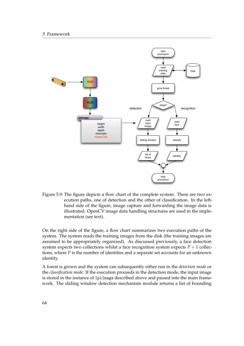
5 Framework
start
procedure
read
training
dataDisk
grow forest
stage?
read
input
image
read
face
sliding window classify
list of
facesidentity
stop
procedure
detection recognition
heightwidthdepth
channelsimageData
IplImage
YUV
RGB
Figure 5.9: The figure depicts a flow chart of the complete system. There are two ex-ecution paths, one of detection and the other of classification. In the left-hand side of the figure, image capture and forwarding the image data isillustrated. OpenCV image data handling structures are used in the imple-mentation (see text).
On the right side of the figure, a flow chart summarizes two execution paths of thesystem. The system reads the training images from the disk (the training images areassumed to be appropriately organized). As discussed previously, a face detectionsystem expects two collections whilst a face recognition system expects P + 1 collec-tions, where P is the number of identities and a separate set accounts for an unknownidentity.
A forest is grown and the system can subsequently either run in the detection mode orthe classification mode. If the execution proceeds in the detection mode, the input imageis stored in the instance of IplImage described above and passed into the main frame-work. The sliding window detection mechanism module returns a list of bounding
64

5.10 Implementation
boxes predicted to be faces. The faces are cropped and saved.
The framework is re-run for recognition. The detected face is propagated on the forestand the classification results are returned as the identity of the face. It is rarely thecase that we constantly add images to any face detection training data. Similarly, thetraining data for recognition is augmented only in case a new identity is to be learnt.To prevent growing random forests at every run, we have implemented a module tosave the random forests locally. The execution path of the framework does not requireaccess to the training data but to the saved abstract alone.
To visualize grown trees, we use GRAPHVIZ 4, a graph visualization software. As webuild binary trees, we create a digraph with the command:digraph g { node [shape = record,height=.1], where the parameters define theshape of the nodes and the default height. When a child node is instantiated in therandom tree, we use the command:node%d[label = "<f0> %d| <f1> %s |<f2> %s "], where the first two parametersare unique numbers assigned to the node, the third parameter is the compositionin terms of the training data with respect to this node and the fourth parameter is theentropy value of the best test chosen at the node. We assign a global count of the nodescreated to the first two parameters. Figure 5.5 illustrates our design. In the figure, everynode in the displayed random tree is characterized with a global count of the node,the composition and the entropy value of the best test. Subsequently, we monitor theskeleton of the growth, as shown in Figure 5.6, by setting the style attribute to invisand the shape attribute to rectangle. We note that the description of the visualizationas specified above is drawn from the semantics of the DOT language 5.
5.10.2 Software Architecture
We present a general skeleton of our software architecture below. We segment thearchitecture into three parts: image manipulation structures, random tree structuresand parameterization. The images, once read, are converted to the integral imagerepresentation discussed in Section 5.3.3. To access pixels easily, we wrote a wrapper forthe IplImage data structure to use both tri-band images and grayscale images as shownin Figure 5.10. In the figure, the pixel values of the tri-band image or the grayscaleimages can be read with the get methods. The images are converted to an array ofintegers using the recursive definition detailed in Equation 5.10 and Equation 5.11.Each of the N training images are read and stored in the integral image representationas a vector called VectorOfIntegralImages.
4http://www.graphviz.org/5http://www.graphviz.org/doc/info/lang.html
65
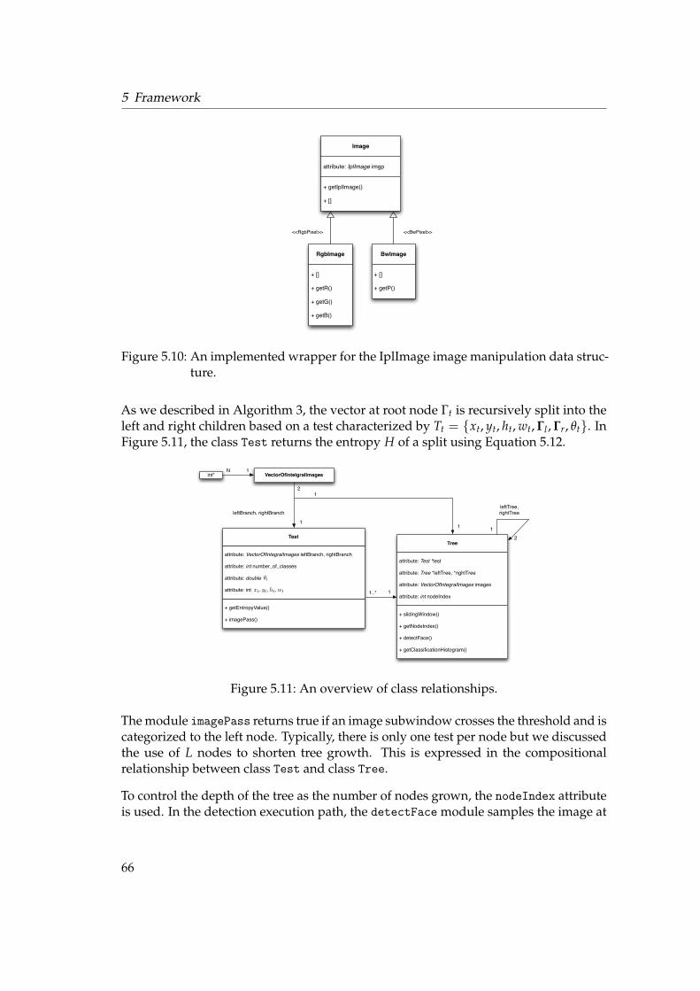
5 Framework
+ getIplImage()
+ []
attribute: IplImage imgp
Image
+ []
+ getR()
+ getG()
+ getB()
RgbImage
<<RgbPixel>>
+ []
+ getP()
BwImage
<<BwPixel>>
Figure 5.10: An implemented wrapper for the IplImage image manipulation data struc-ture.
As we described in Algorithm 3, the vector at root node !t is recursively split into theleft and right children based on a test characterized by Tt = {xt, yt, ht, wt, "l , "r, ,t}. InFigure 5.11, the class Test returns the entropy H of a split using Equation 5.12.
int* VectorOfIntelgralImagesN 1
+ getEntropyValue()
+ imagePass()
attribute: VectorOfIntegralImages leftBranch, rightBranch
attribute: int number_of_classes
attribute: double
attribute: int
Test
2
1
leftBranch, rightBranch
xt, yt, ht, wt
+ slidingWindow()
+ getNodeIndex()
+ detectFace()
+ getClassificationHistogram()
attribute: Test *test
attribute: Tree *leftTree, *rightTree
attribute: VectorOfIntegralImages images
attribute: int nodeIndex
Tree
1
11
2
leftTree,rightTree
1..* 1
!t
Figure 5.11: An overview of class relationships.
The module imagePass returns true if an image subwindow crosses the threshold and iscategorized to the left node. Typically, there is only one test per node but we discussedthe use of L nodes to shorten tree growth. This is expressed in the compositionalrelationship between class Test and class Tree.
To control the depth of the tree as the number of nodes grown, the nodeIndex attributeis used. In the detection execution path, the detectFace module samples the image at
66

5.10 Implementation
different scales and the slidingWindow module iteratively detects faces. In the recogni-tion execution path, the getClassificationHistogram returns the identity.
+ get*()
attribute: string location_training, location_testing
attribute: int minimum_feature_size, maximum_feature_size
attribute: int L, number_of_nodes
attribute: FILE file_list[10]
attribute: int number_of_classes
attribute: double face_map_threshold, merge_window_threshold
attribute: double identity_threshold
ConfigClass
Figure 5.12: The ConfigClass data structure for the parameterization.
We have, to this point, described the image manipulation and the random tree soft-ware data structures. For our parameterization, we consider a separate structure titledConfigClass. Figure 5.12 shows a subset of important attributes. The class is comple-mented with corresponding get modules. The attribute file_list contains the logfiles of the random forests. The main module operates on the basis of the overviewpresented in Figure 5.9. A collection of random trees are grown and the post processingstep effectively aggregates the results from each tree.
67


6 EVALUATIONS
In this chapter, we present evaluations of our framework on face detection and recog-nition. We compare face detection with random forests to the adaptive boosting basedface detector by Viola and Jones [30]. Our evaluations are presented with ROC curvesin Section 6.1. We compare face recognition with random forests to support vectormachines and log-linear models in Section 6.2. The latter evaluations are presentedwith confusion matrices and rank-1 recognition rates, both of which are introducedshortly.
6.1 Face Detection
In this section, we present evaluations on face detection with random forests. In Sec-tion 6.1.1, we introduce ROC curves. In Section 6.1.2 we present our comparisons.
6.1.1 Introduction
The evaluation of a face detection system [30] is typically presented using a receiveroperating characteristics (ROC) curve [27]. The ROC curves is a plot of sensitivityversus 1 - specificity. For a detection system, the number of faces correctly detected areidentified as the benefits of the system. On the other hand, the number of false positivesreturned are identified as costs. ROC curves are influential in analyzing tradeoffsbetween benefits and costs.
The ROC curves are plotted with true positive rate (TPR) on the Y-axis and false positiverate (FPR) on the X-axis. To recapitulate, the true positive rate is calculated as,
True Positive Rate =true positives
true positives + false negatives
=number of faces detected
total number of faces in the input image(6.1)
where Equation 6.1 is the detection accuracy previously discussed in Chapter 3. This isthe sensitivity of the detection system.
69
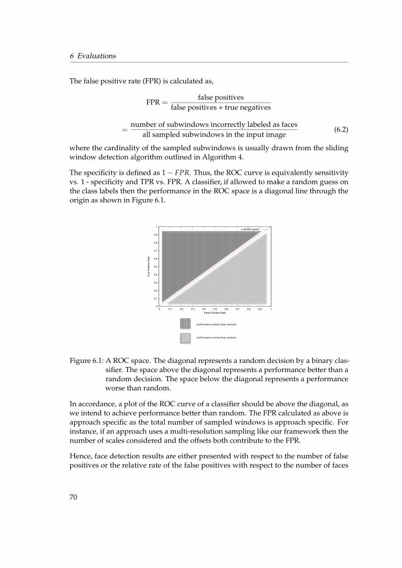
6 Evaluations
The false positive rate (FPR) is calculated as,
FPR =false positives
false positives + true negatives
=number of subwindows incorrectly labeled as faces
all sampled subwindows in the input image(6.2)
where the cardinality of the sampled subwindows is usually drawn from the slidingwindow detection algorithm outlined in Algorithm 4.
The specificity is defined as 1' FPR. Thus, the ROC curve is equivalently sensitivityvs. 1 - specificity and TPR vs. FPR. A classifier, if allowed to make a random guess onthe class labels then the performance in the ROC space is a diagonal line through theorigin as shown in Figure 6.1.
0
0.1
0.2
0.3
0.4
0.5
0.6
0.7
0.8
0.9
1
0 0.1 0.2 0.3 0.4 0.5 0.6 0.7 0.8 0.9 1
Tru
e P
ositiv
e R
ate
False Positive Rate
a random guess
performance better than random
performance worse than random
Figure 6.1: A ROC space. The diagonal represents a random decision by a binary clas-sifier. The space above the diagonal represents a performance better than arandom decision. The space below the diagonal represents a performanceworse than random.
In accordance, a plot of the ROC curve of a classifier should be above the diagonal, aswe intend to achieve performance better than random. The FPR calculated as above isapproach specific as the total number of sampled windows is approach specific. Forinstance, if an approach uses a multi-resolution sampling like our framework then thenumber of scales considered and the offsets both contribute to the FPR.
Hence, face detection results are either presented with respect to the number of falsepositives or the relative rate of the false positives with respect to the number of faces
70

6.1 Face Detection
in the input image. In the latter, Equation 6.2 is rewritten as,
FPR =number of subwindows incorrectly labeled as faces
total number of faces in the input image(6.3)
It can be derived that the FPR calculated thus is in the range [0 : Z], where
Z =all sampled subwindows
total number of faces in the input image
and Z is the right most point in the X-axis of the ROC curve plot.
ROC curves help us measure the highest achievable detection accuracy with respect toan allowed number of false positives. Global parameters, such as the number of nodesgrown and the face map threshold, are varied to measure the detection accuracy andthe accompanying false positives count. The responses are plotted. If the algorithmallows every subwindow to be classified as a face then the FPR will take the maximumvalue but the TPR will be 1.0. This is the final point in the ROC curve where we have100% detection accuracy at the cost of every non-face falsely labeled as a face.
6.1.2 ROC Curve Plots
We evaluate the performance of our detection system against the adaptive boostingbased face detector proposed by Viola and Jones [30]. The Viola and Jones detectoroffers one of the most impressive detection performances [29, 30]. It is also freelyavailable as a module of the OpenCV library. Configuration files trained to detectfaces are also supplied as part of the OpenCV installation. We note that the suppliedconfiguration files offer the best results.
A clear comparison of the two approaches is only possible under the following condi-tions:
• the approaches are trained on the same training data and
• the results are evaluated under similar conditions on the same test data.
In accordance, we ran experimental analyses on a comprehensive set of training datafreely available (enumerated in Section 4.3.1). The best performances on both randomforests and the adaboost approach was achieved on the Universidad Politecnica deValencia Face database [65]. We consider three subsets for training:
1. C1. The subset has a random selection of 1000 faces and 1000 background images.
2. C2. The subset has a random selection of 4000 faces and 4000 background images.
3. C3. The subset has a random selection of 10000 faces and 10000 backgroundimages.
71

6 Evaluations
The non-faces in each of the subsets were obtained by extracting random patches fromthe images that do not contain any faces and are typical backgrounds. All the trainingimages used are 24 ! 24 pixels in height and width.
The test set is composed of a difficult subset and a randomly chosen subset drawn fromboth the CMU test collection (Section 4.3.2) and the BioID face data set (Figure 4.8). Theformer is composed of faces of varying sizes in complex backgrounds and differentillumination conditions as well as rotated faces. The latter was chosen as it approxi-mately presents typical images that a mobile robot may encounter. The images in theBioID dataset contain faces with the following characteristics:
• slight variations in pose,
• sufficient variations in expressions,
• slight variations in illumination,
• slight variations in the dimension of the faces across the identities and
• typical backgrounds that a mobile robot might encounter such as windows andthe backdrop of a room.
The complete test collection consists of 123 images with a total of 188 faces. Withrespect to this test set, we present the following evaluations for face detection:
1. R1, a ROC curve plot of random forests vs. the adaboost module, both trained onC1.
2. R2, a ROC curve plot of random forests vs. the adaboost module, both trained onC2.
3. R3, a ROC curve plot of random forests vs. the adaboost module, both trained onC3 and the adaboost trained for 6 stages. We refer to the corresponding adaboosttraining as Adaptive Boost #1.
4. R4, a ROC curve plot of random forests vs. the adaboost module, both trained onC3 and the adaboost trained for 9 stages. We refer to the corresponding adaboosttraining as Adaptive Boost #2.
5. R5, a ROC curve plot of random forests trained on C3 vs. the adaboost moduleused with a configuration file supplied as is. We refer to the correspondingadaboost training as Adaptive Boost #3.
An important disparity between the approaches is the training time. As we discussedearlier, the adaboost face detector builds cascades of binary classifiers. Each attentionalcascade reduces the false positive rate further. In accordance, the training time increasesfor each additional stage. Training the adaboost module for R3 to 6 stages requires 5days on an Intel Core 2 Duo processor equipped with 2 Gigabytes of RAM. Training theadaboost module for R3 to 8 stages requires 7 days on an Opteron machine equippedwith 16 Gigabytes of RAM. In comparison, training random forests on R3 for a node
72
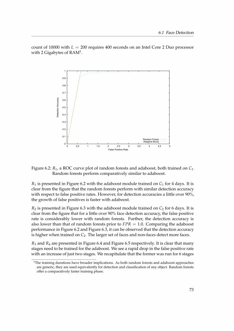
6.1 Face Detection
count of 10000 with L = 200 requires 400 seconds on an Intel Core 2 Duo processorwith 2 Gigabytes of RAM1.
0
0.1
0.2
0.3
0.4
0.5
0.6
0.7
0.8
0.9
1
0 0.5 1 1.5 2 2.5 3 3.5 4 4.5 5
Dete
ctio
n Ac
cura
cy
False Positive Rate
Random ForestAdaptive Boost
Figure 6.2: R1, a ROC curve plot of random forests and adaboost, both trained on C1.Random forests perform comparatively similar to adaboost.
R1 is presented in Figure 6.2 with the adaboost module trained on C1 for 4 days. It isclear from the figure that the random forests perform with similar detection accuracywith respect to false positive rates. However, for detection accuracies a little over 90%,the growth of false positives is faster with adaboost.
R2 is presented in Figure 6.3 with the adaboost module trained on C2 for 6 days. It isclear from the figure that for a little over 90% face detection accuracy, the false positiverate is considerably lower with random forests. Further, the detection accuracy isalso lower than that of random forests prior to FPR = 1.0. Comparing the adaboostperformance in Figure 6.2 and Figure 6.3, it can be observed that the detection accuracyis higher when trained on C2. The larger set of faces and non-faces detect more faces.
R3 and R4 are presented in Figure 6.4 and Figure 6.5 respectively. It is clear that manystages need to be trained for the adaboost. We see a rapid drop in the false positive ratewith an increase of just two stages. We recapitulate that the former was run for 6 stages
1The training durations have broader implications. As both random forests and adaboost approachesare generic, they are used equivalently for detection and classification of any object. Random forestsoffer a comparatively faster training phase.
73

6 Evaluations
0
0.1
0.2
0.3
0.4
0.5
0.6
0.7
0.8
0.9
1
0 0.5 1 1.5 2 2.5 3 3.5 4 4.5 5
De
tectio
n A
ccu
racy
False Positive Rate
Random ForestAdaptive Boost
Figure 6.3: R2, a ROC curve plot of random forests and adaboost, both trained onC2. Random forests present a higher detection accuracy for lower falsepositives.
and the latter for 8. Random forests slightly outperform the adaboost approaches tillapproximately 91% detection accuracy. It is reported that the false positive rate isexpected to drop to very low values with as many as 25 stages 2.
We finally present R5 in Figure 6.6. From the figure, we observe a slightly betterperformance of Adaptive Boost #3 with respect to random forests. The random forests,on the other hand, perform better than Adaptive Boost #2 and Adaptive Boost #1, aswas concluded from Figure 6.2 and Figure 6.3. We reiterate that the adaboost approachoffers the best face detection system [30].
Figure 6.7 highlights the detection rates at a higher granularity for a FPR range of [0:1].In the figure, the plot of Adaptive Boost #3 is close to the Y-axis in the figure. This isattributed to the fact that for low detection accuracies, Adaptive Boost #3 yields verylow false positives. It is to be noted that neither Adaptive Boost #1 nor Adaptive Boost#2 perform similarly for the stages we trained them to. It can be concluded from thegraph that for a detection accuracy of over 90%, the false positive rates are roughlyequal for both Adaptive Boost #1 and random forests. For instance, allowing 25 false
2http://groups.google.com/group/OpenCV
74

6.1 Face Detection
0
0.1
0.2
0.3
0.4
0.5
0.6
0.7
0.8
0.9
1
0 0.5 1 1.5 2 2.5 3 3.5 4 4.5 5
Dete
ctio
n Ac
cura
cy
False Positive Rate
Random ForestAdaptive Boost #1
Figure 6.4: R3, a ROC curve plot of random forests and adaboost, both trained on C3.The adaboost was trained to 6 stages.
positives, Adaptive Boost #3 detects 178 and random forests detect 175 out of the 188faces.
One of the principal justifications for the slightly lower performance of random forestwhen compared to Adaptive Boost #3 is that of the post processing phase. The postprocessing phase must effectively merge the detections from both the multi-resolutionsampling and all the random trees. We grow only three random trees for face detectionas we observed the faces get successfully detected in each of the trees. Taking all of themerging strategies discussed in Section 5.6 into account, we found the following stepsto be most effective:
• The individual scale results are merged by considering neighbors from overlap-ping rectangles as outlined in Figure 5.7. The merging procedure used is one thatconsiders a weighted combination described in Equation 5.15. The $ tied to thedetection window with the highest FMP is set to 1 and the remaining are set tovery low values.
• The results of the step above are scaled back to be applicable to the input image.Neighbors are found from overlapping rectangles as above. The biggest rectangleis selected and the others are discarded.
75

6 Evaluations
0
0.1
0.2
0.3
0.4
0.5
0.6
0.7
0.8
0.9
1
0 0.5 1 1.5 2 2.5 3 3.5 4 4.5 5
Dete
ctio
n Ac
cura
cy
False Positive Rate
Random ForestAdaptive Boost #2
Figure 6.5: R4, a ROC curve plot of random forests and adaboost, both trained on C3.The adaboost was trained to 8 stages.
The above merging strategy, although it performs best among other strategies experi-mented with, is error prone. In comparison, the adaboost approach builds a cascadeof classifiers to reduce the false positives in the attentional stages. The initial stages,on the other hand, are very liberal to allow for a large number of detections. Thereseems to be no trivial procedure to accomplish the same for random forests in shortof a direct analogy: growing stages of random forests and forwarding detections fromthe previous stage to the next. Additionally, the detection subwindows suffer fromalignment errors.
Figure 6.8 presents a few of our detections. Minor alignment errors are present in someof the detections. However, if we consider the image highlighted with a blue border,we note that the second detection (orange subwindow) is badly aligned3. In the imagehighlighted with a turquoise border, we note a false positive. In the image highlightedwith a purple border, we note a false negative, i.e. a face is not detected at all.
We aim to the address the above in our future work (Chapter 7) and conclude with theremark that random forests offer extremely competitive results with respect to the bestface detection system in literature.
3Our evaluations do not nominate the same as a correctly detected face.
76

6.2 Face Recognition
0
0.1
0.2
0.3
0.4
0.5
0.6
0.7
0.8
0.9
1
0 0.5 1 1.5 2 2.5 3 3.5 4 4.5 5
Dete
ctio
n Ac
cura
cy
False Positive Rate
Random ForestAdaptive Boost #1Adaptive Boost #2Adaptive Boost #3
Figure 6.6: R5, a ROC curve plot of random forests and adaboost modules. AdaptiveBoost #1 is adaboost trained on C3 to 6 stages. Adaptive Boost #2 is ad-aboost trained on C4 to 8 stages. Adaptive Boost #3 is the performancewith a configuration file for face detection provided as part of the OpenCVinstallation.
6.2 Face Recognition
To present our face recognition results we use the simplified construction of our recog-nition framework. Namely, we build a separate random forest trained on the P classcollection. We present all our evaluations on 4000 nodes and L = 1000. We report thatgrowing a random tree to 4000 nodes with L = 1000 requires 75 seconds. Growing arandom tree to 1000 nodes with L = 200 requires 3 seconds.
6.2.1 Testing Framework
In Chapter 4, we discussed the FERET evaluation as one of the benchmarks used bymost face recognition systems. However, the FERET evaluation is composed primarilyof one training image and one probe image. Due to the training nature of randomforests, we need more training images. Thus, we present three separate evaluation col-lections below. Needless to say, the training data D and the test data T are completely
77

6 Evaluations
0
0.1
0.2
0.3
0.4
0.5
0.6
0.7
0.8
0.9
1
0 0.1 0.2 0.3 0.4 0.5 0.6 0.7 0.8 0.9 1
Dete
ctio
n Ac
cura
cy
False Positive Rate
Random ForestAdaptive Boost #1Adaptive Boost #2Adaptive Boost #3
Figure 6.7: R5, a ROC curve plot of random forests and adaboost modules. The plot islimited in the FPR range of [0:1].
disjoint, i.e. D . T = Ø.
• T1, 4 identities randomly drawn from the Universidad Politecnica de ValenciaFace database [65] database with the following training data composition is D ={(188, 0), (164, 1), (92, 2), (92, 3)}, where D is the training data that has 188 facesfor identity 0, 164 faces for identity 1 etc. The test data composition is T ={(14, 0), (14, 1), (14, 2), (14, 3)}.
• T2, 7 identities randomly drawn from the BioID database. We are not awareof any identity annotation of the BioID face database. We thus manually sep-arated the database based on different identities and selected seven identitieswith the highest number of images. The training data composition is D ={(65, 0), (59, 1), (67, 2), (72, 3), (37, 4), (65, 5), (99, 6)}. The test data compositionis T = {(8, 0), (2, 1), (2, 2), (5, 3), (15, 4), (9, 5), (0, 6)}. We note that a subset of thefaces in T2 were supplied with their respective backgrounds as part of the testcollection for the ROC plots presented previously.
• T3, to probe the performance of our recognition framework when the numberof training are less, we consider five randomly chosen identities from the YaleDatabase [67]. The training data composition is D = {(9, 0), (7, 1), (8, 2), (9, 3), (9, 4)}.The test data composition is T = {(2, 0), (4, 1), (3, 2), (2, 3), (2, 4)}.
78
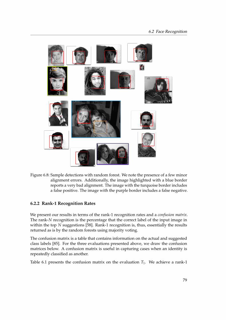
6.2 Face Recognition
Figure 6.8: Sample detections with random forest. We note the presence of a few minoralignment errors. Additionally, the image highlighted with a blue borderreports a very bad alignment. The image with the turquoise border includesa false positive. The image with the purple border includes a false negative.
6.2.2 Rank-1 Recognition Rates
We present our results in terms of the rank-1 recognition rates and a confusion matrix.The rank-N recognition is the percentage that the correct label of the input image inwithin the top N suggestions [58]. Rank-1 recognition is, thus, essentially the resultsreturned as is by the random forests using majority voting.
The confusion matrix is a table that contains information on the actual and suggestedclass labels [85]. For the three evaluations presented above, we draw the confusionmatrices below. A confusion matrix is useful in capturing cases when an identity isrepeatedly classified as another.
Table 6.1 presents the confusion matrix on the evaluation T1. We achieve a rank-1
79

6 Evaluations
0 1 2 30 14 0 0 01 0 14 0 02 6 0 8 03 1 0 0 13
Table 6.1: A confusion matrix on the evaluation collection T1. Rank-1 recognition rateof 87.5%.
0 1 2 3 4 50 5 0 0 0 0 31 1 1 0 0 0 02 0 0 2 0 0 03 0 0 0 5 0 04 1 0 0 0 14 05 0 0 0 0 0 5
Table 6.2: A confusion matrix on the evaluation collection T2. Rank-1 recognition rateof 86.5%.
recognition rate of 87.5%. The rank-1 recognition can be calculated directly from theconfusion matrix using:
rank-1 recognition =sum of the diagonal elements
sum of the rows or sum of the columns
Table 6.2 presents the confusion matrix on the evaluation T2. We achieve a rank-1recognition rate of 86.5%. Finally, the evaluation of random forests with very littletraining data is presented in Table 6.3. We achieve a rank-1 recognition rate of 85%where 11 of the 13 test images are correctly classified.
0 1 2 3 40 2 0 0 0 01 1 3 0 0 02 0 1 2 0 03 0 0 0 2 04 0 0 0 0 2
Table 6.3: A confusion matrix on the evaluation collection T3. Rank-1 recognition rateof 85.0%.
80

6.2 Face Recognition
0 1 2 30 14 0 0 01 0 14 0 02 0 3 11 03 0 0 0 14
0 1 2 30 14 0 0 01 0 14 0 02 0 2 12 03 0 0 0 14
Figure 6.9: Left:T1 with log-linear models with rank-1 recognition of 94.6%. Right:T1with SVM with rank-1 recognition of 96.4%.
0 1 2 3 4 50 8 0 0 0 0 01 1 1 0 0 0 02 0 0 1 0 1 03 0 0 0 5 0 04 0 0 0 0 15 05 0 0 0 0 0 5
0 1 2 3 4 50 8 0 0 0 0 01 1 1 0 0 0 02 0 0 2 0 0 03 0 0 0 5 0 04 0 0 0 0 15 05 0 0 0 0 0 5
Figure 6.10: Left:T2 with log-linear models with rank-1 recognition of 94.6%. Right:T1with SVM with rank-1 recognition of 97.3%.
To compare our evaluations to important approaches used in literature, we considerface recognition using support vector machines and log-linear models. Support vectormachines were previously presented in Section 4.2 and the corresponding illustrationin Figure 4.3. We use the LIBSVM [62, 63] library for support vector machine basedrecognition. The values for C and * were drawn using cross-validation. The valuesobtained thus are used to build P(P' 1)/2 SVM with the complete training data. Weuse an implementation by Deselaers et al. [86] for building our log linear models. Wepresent the confusion matrices and corresponding recognition rates here.
Figure 6.9 presents the rank-1 recognition rates on T1 using log-linear models and SVM.Figure 6.10 presents the rank-1 recognition rates on T2 using log-linear models and
0 1 2 3 40 2 0 0 0 01 0 4 0 0 02 0 0 3 0 03 0 0 0 2 04 0 0 0 0 2
0 1 2 3 40 2 0 0 0 01 0 4 0 0 02 0 1 2 0 03 0 0 0 2 04 0 0 0 0 2
Figure 6.11: Left:T3 with log-linear models with rank-1 recognition of 100.0%. Right:T3with SVM with rank-1 recognition of 92.3%.
81
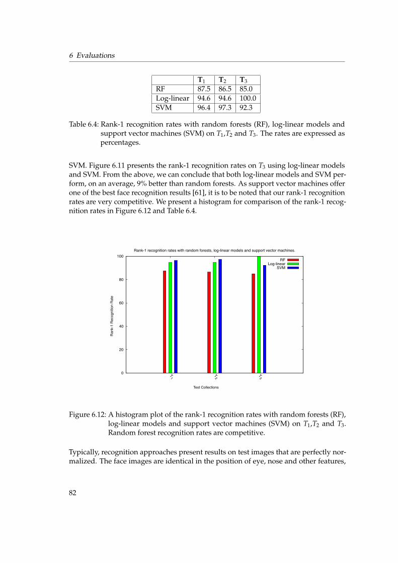
6 Evaluations
T1 T2 T3RF 87.5 86.5 85.0Log-linear 94.6 94.6 100.0SVM 96.4 97.3 92.3
Table 6.4: Rank-1 recognition rates with random forests (RF), log-linear models andsupport vector machines (SVM) on T1,T2 and T3. The rates are expressed aspercentages.
SVM. Figure 6.11 presents the rank-1 recognition rates on T3 using log-linear modelsand SVM. From the above, we can conclude that both log-linear models and SVM per-form, on an average, 9% better than random forests. As support vector machines offerone of the best face recognition results [61], it is to be noted that our rank-1 recognitionrates are very competitive. We present a histogram for comparison of the rank-1 recog-nition rates in Figure 6.12 and Table 6.4.
0
20
40
60
80
100
T1
T2
T3
Rank-1 recognition rates with random forests, log-linear models and support vector machines.
RFLog-linear
SVM
Rank-1
Recognitio
n R
ate
Test Collections
Figure 6.12: A histogram plot of the rank-1 recognition rates with random forests (RF),log-linear models and support vector machines (SVM) on T1,T2 and T3.Random forest recognition rates are competitive.
Typically, recognition approaches present results on test images that are perfectly nor-malized. The face images are identical in the position of eye, nose and other features,
82

6.2 Face Recognition
both in the training data and the test collection. However, in a mobile robot, we cannot expect perfectly normalized faces. As a result, the test images in T1, T2 and T3were obtained automatically using Adaptive Boost #3. We discussed previously inSection 6.1.2 that although random forests detect faces comparatively to adaboost onthe ROC curve plots, the former suffers with considerable alignment errors. As ourrecognition models expect the location of facial features at approximately relative spa-tial locations, the recognition rates are low when faces directly cropped from randomforest detections are used. Jones and Viola [58] report that the faces detected using theadaptive boost face detector are additionally normalized with fixed eye positions. Ourresults above, however, are directly drawn from the extent and position as returned byAdaptive Boost #3.
0
20
40
60
80
100
T2
T3
Rank-1 recognition rates with random forests, log-linear models and support vector machines.
RFLog-linear
SVM
Rank-1
Recognitio
n R
ate
Test Collections
Figure 6.13: A histogram plot of the rank-1 recognition rates with random forests (RF),log-linear models and support vector machines (SVM) on T2 and T3. Thetest data was drawn from detections as returned by the random forestdetection framework presented in Section 5.5.
The histogram in Figure 6.13 reflects the recognition performance on using the detec-tions from random forests directly. We present rank-1 recognition rates on only T2 andT3 as all the images from T1 are completely normalized. We reiterate that the trainingimages are the same as those used for Figure 6.12. The results are also presented as a ta-ble in Table 6.5. Here, we observe that random forests perform well on T3 as comparedto T2. This is attributed to the fact that the detection in T2 suffer from higher alignment
83

6 Evaluations
T2 T3RF 13.7 53.4Log-linear 25.5 30.8SVM 31.37 30.76
Table 6.5: Rank-1 recognition rates with random forests (RF), log-linear models andsupport vector machines (SVM) on T2 and T3. The test data was drawn fromdetections as returned by the random forest detection framework presentedin Section 5.5. The rates are expressed as percentages.
error rates.
6.2.3 Unknown Identity
Face recognition literature does not clearly model the identification of an unknownidentity. The task is challenging as most approaches, typically, search for the likelihoodof an input face recognized as an identity $p. The result of this search is one of theknown identities. A heuristically chosen threshold is introduced to nominate the inputface as the corresponding identity or as unknown. Turk and Pentland [39], for instance,introduce a threshold with which the vector of weights from the eigenface frameworkare compared to determine if the face is known or unknown. We evaluate an approachto the identification of unknown identities with random forests below.
In Section 5.7, we outlined a procedure to identify strangers. We model our recognitionframework as a P + 1 class problem where the additional class contains a collection offaces images of different identities. If an input face is recognized as belonging to thisclass, we designate the face to be unknown. We present our evaluations on T1. Our testapproach is as follows. To begin with, T1 is composed of training images and test im-ages of four identities. We created a separate collection of 188 face images of identitiesrandomly sampled from the entire set of identities not considered in {$0, $1, $2, $3}.We denote the same as $P+1. We now iteratively replace one of the four identitieswith $P+1 and measured the corresponding recognition rates. For instance, in the firstrun, we replace the training images for $0 with $P+1. We now measure the (i) rank-1recognition on the test images for $1,2,3 and (ii) rank-1 recognition on the test image for$0. The first measurement, m1, investigates the decrease in recognition on introducinga training collection with a wide variety of face images. The second measurement, m2,investigates the nomination of an unknown face as an unknown identity, in this case,$0. Thus, in our experimental framework, an ideal recognition would categorize eachtest image in the exact same training data index.
Figure 6.14 plots the results. In the figure, the red color plot denotes that the trainingdata composition is {$P+1, $1, $2, $3} (there is no training data for identity 0). Test
84
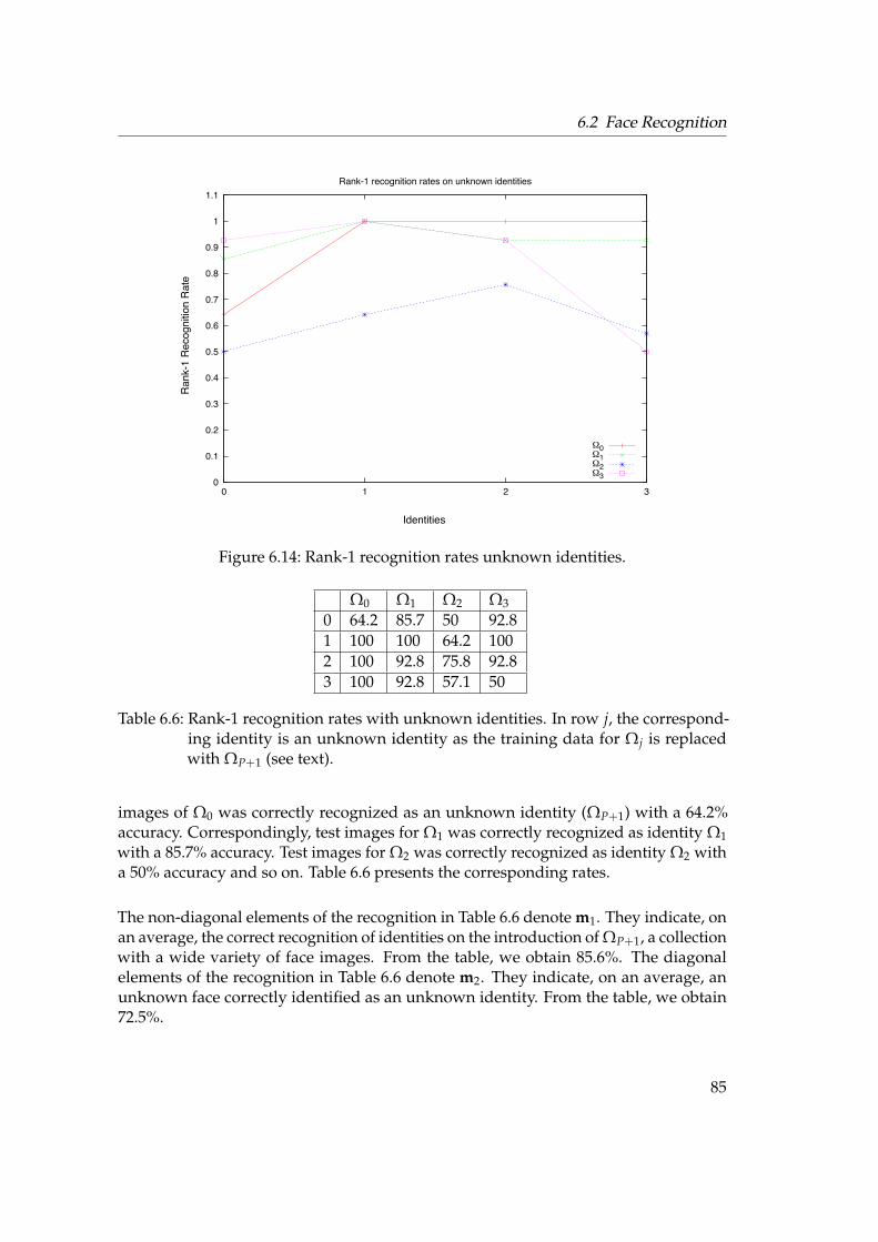
6.2 Face Recognition
0
0.1
0.2
0.3
0.4
0.5
0.6
0.7
0.8
0.9
1
1.1
0 1 2 3
Rank-1 recognition rates on unknown identities
!0!1!2!3
Rank-1
Recognitio
n R
ate
Identities
Figure 6.14: Rank-1 recognition rates unknown identities.
$0 $1 $2 $30 64.2 85.7 50 92.81 100 100 64.2 1002 100 92.8 75.8 92.83 100 92.8 57.1 50
Table 6.6: Rank-1 recognition rates with unknown identities. In row j, the correspond-ing identity is an unknown identity as the training data for $j is replacedwith $P+1 (see text).
images of $0 was correctly recognized as an unknown identity ($P+1) with a 64.2%accuracy. Correspondingly, test images for $1 was correctly recognized as identity $1with a 85.7% accuracy. Test images for $2 was correctly recognized as identity $2 witha 50% accuracy and so on. Table 6.6 presents the corresponding rates.
The non-diagonal elements of the recognition in Table 6.6 denote m1. They indicate, onan average, the correct recognition of identities on the introduction of $P+1, a collectionwith a wide variety of face images. From the table, we obtain 85.6%. The diagonalelements of the recognition in Table 6.6 denote m2. They indicate, on an average, anunknown face correctly identified as an unknown identity. From the table, we obtain72.5%.
85
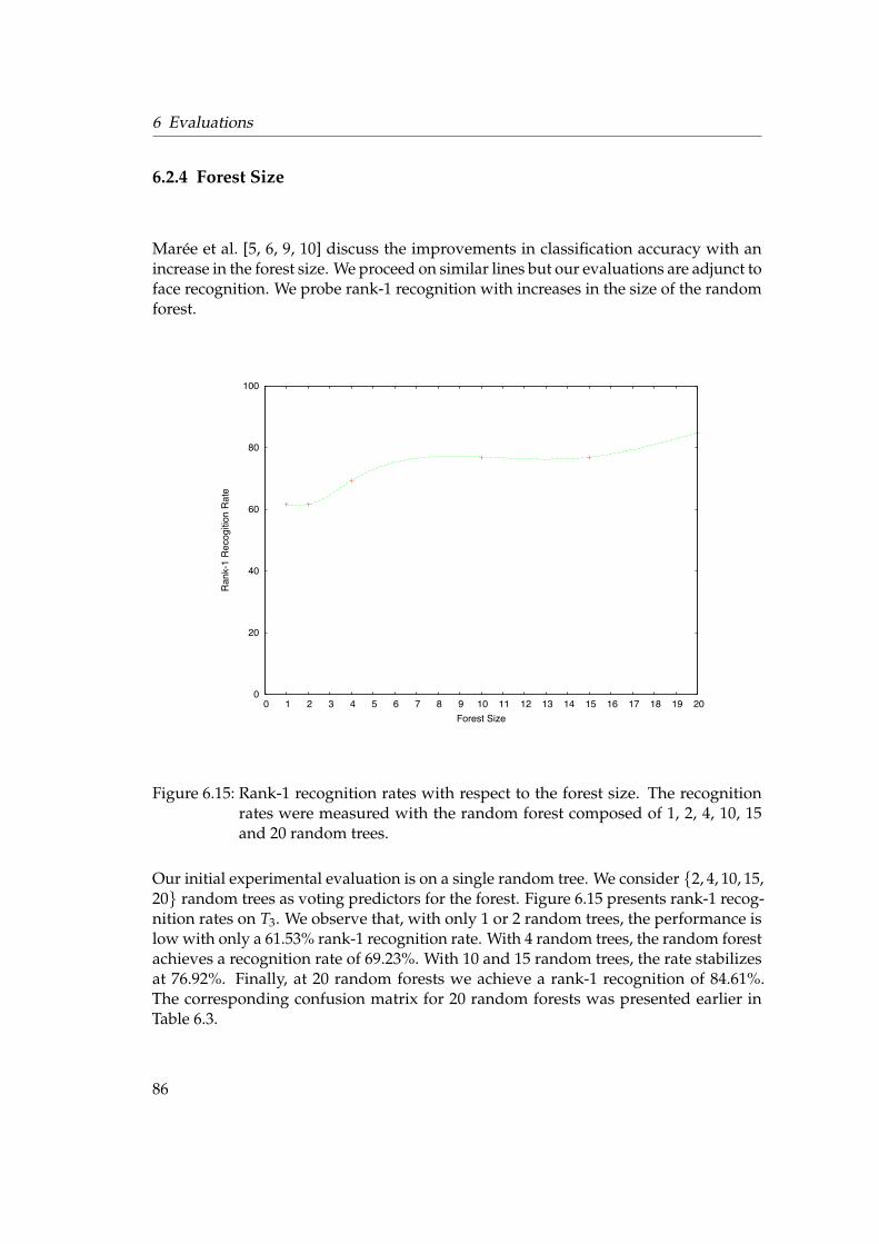
6 Evaluations
6.2.4 Forest Size
Marée et al. [5, 6, 9, 10] discuss the improvements in classification accuracy with anincrease in the forest size. We proceed on similar lines but our evaluations are adjunct toface recognition. We probe rank-1 recognition with increases in the size of the randomforest.
0
20
40
60
80
100
0 1 2 3 4 5 6 7 8 9 10 11 12 13 14 15 16 17 18 19 20
Rank
-1 R
ecog
ition
Rate
Forest Size
Figure 6.15: Rank-1 recognition rates with respect to the forest size. The recognitionrates were measured with the random forest composed of 1, 2, 4, 10, 15and 20 random trees.
Our initial experimental evaluation is on a single random tree. We consider {2, 4, 10, 15,20} random trees as voting predictors for the forest. Figure 6.15 presents rank-1 recog-nition rates on T3. We observe that, with only 1 or 2 random trees, the performance islow with only a 61.53% rank-1 recognition rate. With 4 random trees, the random forestachieves a recognition rate of 69.23%. With 10 and 15 random trees, the rate stabilizesat 76.92%. Finally, at 20 random forests we achieve a rank-1 recognition of 84.61%.The corresponding confusion matrix for 20 random forests was presented earlier inTable 6.3.
86

6.3 Summary
0 1 2 30 5 1 1 01 0 7 0 02 0 0 7 03 0 0 0 7
Table 6.7: A confusion matrix on KBSG Face Database. Rank-1 recognition rate of92.86%.
6.2.5 KBSG Face Database
Our proposal and our motivation was towards a face processing system for mobilerobots. The KBSG Face Database was presented in Figure 4.7. The database was cre-ated with the Firewire camera used with the RWTH Aachen Robocup@Home mobilerobots [73]. The database is representative of the interaction between the robot andhuman subjects as the images are with different illumination conditions, typical back-grounds, side profiles, variable distances between the subjects and the camera.
We used Adaptive Boost #3 directly to crop the faces. We used the image processinglibraries to universally crop and scale the faces to 48! 48. The KBSG database consistsof 4 identities with 30 faces each. We divide the collection to 23 faces for training and 7faces for testing. We report that 26 of the 28 images were accurately recognized, i.e. arank-1 recognition rate of 92.86%. The corresponding confusion matrix is presented inTable 6.7. We note that we do not present recognition on the KBSG Face Database withSVM and log-linear models as we are only interested in the accuracy achieved with ourrandom forest implementation to be deployed on the RWTH RoboCup@Home robots.A comparison of recognition accuracies to SVM and log-linear models have alreadybeen reviewed earlier.
The results presented uses a forest of 20 random trees, with each tree grown to a depthof 3000 nodes. Further, we set L = 1000. The training time for the forest is 14 minutes.However, to learn new identities, we need a fast training framework, especially, to beapplicable to the RoboCup@Home competitions. We thus grew only 3 random trees,each grown to a depth of 800 nodes and L = 50. We report the forest trains and returnsrecognition results in 1 millisecond. The resulting rank-1 recognition rate is 83.3%.
6.3 Summary
In this chapter, we presented comparative evaluations of face detection and recognitionwith random forests. Detection with random forests was compared to an adaptive
87

6 Evaluations
boosting based face detection systems. ROC curve plots were presented on detectionwith random forests and 3 adaptive boosting training configurations.
Recognition with random forests was compared to SVM and log-linear models. Rank-1recognition rates were presented on three test collections. Additionally, rank-1 recogni-tion rates with random forests were presented on the KBSG Face Database that capturestypical image scenarios that a mobile robot will encounter.
Lastly, we presented improvements in classification accuracy on increasing the size ofthe forest. In the next chapter, we draw our conclusions. We briefly summarize theevaluations and discuss future work.
88

7 CONCLUSION AND FUTURE WORK
7.1 Conclusions
Our thesis presents an integrated framework to the detection, recognition and learningof faces with random forests. Random forests are structurally homogenous to classicaldecision trees but randomize the decision criteria. Random forests sample randomrectangular regions and learn features from training data. We have an implementationof our framework that is compared to state-of-the-art approaches. Particularly, wecompare the performance of face detection with random forests to adaptive boosting.Random forests outperform adaptive boosting when they are trained on the samedata. Random forests perform comparatively to adaptive boosting using the trainingconfiguration supplied as part of the OpenCV installation.
We however note that face detection with random forests suffers from alignment errors.The alignment errors are not tied theoretically to random forests but lie in the errorprone merging techniques developed. Merging is influenced by our search for theneighbor range. If the neighbor range is large, multiple faces in the immediate vicinitywill be falsely considered to be the same face. If the neighbor range is small, multiplesubwindows for the same face collected from the multi-resolution analysis and multipletrees will be falsely considered as multiple faces. Thus, we are typically left with a largenumber of nominated detections in neighboring locations making our post-processingnon-trivial.
We presented comparisons of face recognition with random forests to face recognitionwith SVM and log-linear models. We considered 3 test collections and observed thatrandom forests performed within a range of 9%, on average, to both SVM and log-linearmodels.
A critical characteristic of random forests is the training time. Due to the fact thatcompletely random features are sampled, the random tree growth is fast. We reportedin Section 6.2.5 that the training of 3 random trees to a depth of 800 nodes with L =50 takes a millisecond. This feature allows the rebuilding of trees in feasible time.A critical parameter is the forest size. Allowing an increase in the number of treesgrown increases the classification accuracy and training time. A tradeoff is necessarydepending on the time constraints. We have shown that with 20 random trees, highclassification rates are obtained.
89

7 Conclusion and Future work
We have also described two approaches to the realization of our overall framework.The first is building a random forest on the two-class face detection training data andgrowing the same further, for recognition and the introduction of a new identity. Thesecond and simpler approach considers a separate forest for detection and a separateforest for recognition. On the introduction of a new identity, the forest for recognitionis either rebuilt or grown further.
We present a brief overview of our results in Table 7.1. The table presents our concernswith the detection of faces with random forests and its comparative performance toadaptive boosting training configurations. Additionally, rank-1 recognition rates onthe KBSG Face Database is 92.86%, rendering the same to be sufficiently accurate to bedeployed.
Task Tool Conclusions
Face Detection ROC Curveplot
From Section 6.1.2 and Figure 6.6:• RF outperform adaboost with same train-
ing data.
• RF perform comparatively to adaboostwith installed training configuration.
• RF results present non trivial merging pro-cedure.
• RF suffer from alignment errors.
• RF training is fast.
Face Recognition Rank-1recognitionrates
T1 T2 T3RF 87.5 86.5 85.0Log-linear 94.6 94.6 100.0SVM 96.4 97.3 92.3
Table 7.1: A summary of the evaluations on face detection and recognition with randomforests.
In summary, we have presented, reviewed and realized an integrated framework forthe detection, recognition and learning of human faces with random forests for mobilerobots which fulfills our requirements aimed at.
90

7.2 Future Work
7.2 Future Work
Our work was motivated and is towards a face processing system on a mobile robot.While we present fast training times with random forests, we are yet to ascertain if arandom forest framework offers the best run-time deployment. Specifically, we intendto verify the following:
• Does detection with random forests offer an acceptable detection time versusaccuracy trade-off with the mobile robot operating in a dynamic environment?We intend to probe the possibility of achieving satisfactory and fast detection ofhuman faces as the mobile robot is carrying out its typical tasks.
• Does recognition with random forests offer an acceptable recognition time versusaccuracy trade-off in similar conditions as above?
• Is the face learning framework fast enough to render a natural experience? Sp-ecifically, we discussed our intention of the framework made applicable in theRoboCup@Home competitions. The RoboCup@Home necessitates a rapid learn-ing of new identities. To recapitulate, the face learning framework can be real-ized either by growing the forest further or rebuilding the trees. If we realize theframework by rebuilding the trees, we intend to investigate a trade-off betweenthe number of trees and the recognition accuracy in this scenario. If we realizethe framework by growing the trees further, we intend to investigate a trade-offbetween the number of trees to grow further and the recognition accuracy.
• We intend to ascertain the benefits in terms of speed, simplicity, memory effi-ciency of a unified framework as opposed to individual implementations of facedetection and recognition systems.
We previously discussed that the random forest framework is generic. It is thus aninteresting extension to consider the detection and recognition of any general object,such as a cup, in complex backgrounds. The RWTH Aachen RoboCup@Home robotsare already equipped with a speech recognition system [73, 87]. Relaying informationfrom the speech component to recognize humans and objects is a very important ex-tension.
We conclude with the fact that our integrated approach to the detection, recognitionand learning of human faces can be modeled to the detection and recognition of anygeneric object. Further, the framework presented allows the possibility of includingextensions that will lead to an improved social interaction between humans and robots.Lastly, our detections and recognition results, independently, are extremely competitiveto the best detection and recognition results published.
91


8 NOTATION
This section serves as a reference to the common symbols used in our work.
Symbol Name Description
% Real Space space of all real numbers
!N1 data for training defined as {!1, . . . , !N}
cp1 Class Labels class labels defined as {c1, . . . , cp}
D Training Data defined as D = {(!n, cp) : n = 1, . . . , N; p = 1, . . . , P}
$p Identity p is a shorthand symbol for an identity
! Average Face the average of the training images
!p the average of the training images for an identity $p
" denotes a set of training images ("l , "r, etc. )
f Filter defined as f (!) : ! #$ %M&
h Classifier defined as h(!) : ! #$ p, where p is the class label
C Correlation Matrix defined as C = 1N
N
#n=1
(!n ' !)(!n ' !)T
S Scatter Matrix defined as S =N
#n=1
(!n ' !)(!n ' !)T
93


BIBLIOGRAPHY
[1] L. Breiman, “Random forests,” Machine Learning, vol. 45, no. 1, pp. 5–32, 2001.
[2] “Robocup@Home,” [online]. Available from: http://www.ai.rug.nl/robocupathome/ [cited 2008-03-26].
[3] T. van der Zant and T. Wisspeintner, “Robocup x: A proposal for a new leaguewhere robocup goes real world.,” in RoboCup, pp. 166–172, 2005.
[4] S. Schiffer, A. Ferrein, and G. Lakemeyer, “Football is coming home,” in Proc.of International Symposium on Practical Cognitive Agents and Robots, University ofWestern Australia Press, 2006.
[5] R. Marée, P. Geurts, J. Piater, and L. Wehenkel, “A generic approach for imageclassification based on decision tree ensembles and local sub-windows,” in Proc.6th Asian Conference on Computer Vision (ACCV), Jan 2004.
[6] R. Marée, P. Geurts, J. Piater, and L. Wehenkel, “Decision trees and random sub-windows for object recognition,” in ICML workshop on Machine Learning Techniquesfor Processing Multimedia Content (MLMM2005), 2005.
[7] P. Geurts, D. Ernst, and L. Wehenkel, “Extremely randomized trees,” MachineLearning, vol. 36, no. 1, pp. 3–42, 2006.
[8] P. Geurts, D. deSeny, M. Fillet, M. Meuwis, M. Malaise, M. Merville, and L. We-henkel, “Proteomic mass spectra classification using decision tree based ensem-ble methods,” Bioinformatics, vol. 21, no. 14, pp. 3138–3145, 2005.
[9] R. Marée, P. Geurts, and L. Wehenkel, “Random subwindows and extremelyrandomized trees for image classification in cell biology,” To appear in BMC CellBiology supplement on Workshop of Multiscale Biological Imaging, Data Mining andInformatics, 2007.
[10] R. Marée, P. Geurts, J. Piater, and L. Wehenkel, “Random subwindows for robustimage classification.,” in CVPR (1), pp. 34–40, 2005.
[11] V. Lepetit, P. Lagger, and P. Fua, “Randomized trees for real-time keypoint recog-nition,” in CVPR ’05: Proceedings of the 2005 IEEE Computer Society Conference onComputer Vision and Pattern Recognition (CVPR’05) - Volume 2, (Washington, DC,USA), pp. 775–781, IEEE Computer Society, 2005.
[12] F. Moosmann, B. Triggs, and F. Jurie, “Fast discriminative visual codebooks us-ing randomized clustering forests,” in Advances in Neural Information Processing
95

Bibliography
Systems 19 (B. Schölkopf, J. Platt, and T. Hoffman, eds.), pp. 985–992, Cambridge,MA: MIT Press, 2007.
[13] P. Yin, A. Criminisi, J. Winn, and I. Essa, “Tree-based classifiers for bilayer videosegmentation,” in Proc. IEEE Computer Vision and Pattern Recognition (CVPR),2007.
[14] T. Deselaers, A. Criminisi, J. Winn, and A. Agarwal, “Incorporating on-demandstereo for real time recognition,” in IEEE Conference on Computer Vision and PatternRecognition, (Minneapolis, MN, USA), June 2007.
[15] P. Geurts, A. Blanco, and L. Wehenkel, “Segment and combine approach forbiological sequence classification,” in Proc. IEEE Symposium on ComputationalIntelligence in Bioinformatics and Computational Biology (CIBCB 2005), pp. 194–201,2005.
[16] J. Matas and !. Obdr"álek, “Object recognition methods based on transforma-tion covariant features,” in XII. European Signal Processing Conference EUSIPCO -2004 (F. Hlawatsch, G. Matz, M. Rupp, and B. Wistawel, eds.), (Vienna, Austria),pp. 1333 – 1336, TU Vienna, Sept 2004.
[17] T. M. Mitchell, Machine Learning. New York: McGraw-Hill, 1997.
[18] S. Russell and P. Norvig, Artificial Intelligence: A Modern Approach. Upper SaddleRiver, NJ, USA: Prentice Hall, Inc., 1996.
[19] L. Breiman, “Bagging predictors,” Machine Learning, vol. 24, pp. 123–140, Septem-ber 1994.
[20] L. Breiman, J. Friedman, R. Olsen, and C. Stone, Classification and Regression Trees.Monterey, CA: Wadsworth and Brooks, 1984.
[21] T. Ho, “Random decision forest,” in Proc. of the 3rd Int’l Conf. on Document Analysisand Recognition, pp. 278–282, August 1995.
[22] T. Ho, “The random subspace method for constructing decision forests,” IEEETrans. Pattern Anal. Mach. Intell., vol. 20, no. 8, pp. 832–844, 1998.
[23] E. Nowak, F. Jurie, and B. Triggs, “Sampling strategies for bag-of-features imageclassification,” in European Conference on Computer Vision (4), vol. 3954 of LectureNotes in Computer Science, pp. 490–503, Springer, 2006.
[24] V. Kolmogorov, A. Criminisi, A. Blake, G. Cross, and C. Rother, “Bi-layer segmen-tation of binocular stereo video,” Computer Vision and Pattern Recognition, 2005.CVPR 2005. IEEE Computer Society Conference on, vol. 2, pp. 1186 vol. 2–, 20-25June 2005.
[25] M.-H. Yang, D. J. Kriegman, and N. Ahuja, “Detecting faces in images: A survey,”IEEE Trans. Pattern Anal. Mach. Intell., vol. 24, no. 1, pp. 34–58, 2002.
[26] W. Zhao, R. Chellappa, A. Rosenfeld, and P. Phillips, “Face recognition: A litera-ture survey,” in ACM Computing Surveys, pp. 399–458, 2003.
96

Bibliography
[27] M. H. Zweig and G. Campbell, “Receiver-operating characteristic (roc) plots: afundamental evaluation tool in clinical medicine,” Clin. Chem., pp. 561–577, 1993.
[28] H. Rowley, S. Baluja, and T. Kanade, “Human face detection in visual scenes,” inAdvances in Neural Information Processing Systems (D. S. Touretzky, M. C. Mozer,and M. E. Hasselmo, eds.), vol. 8, pp. 875–881, 1996.
[29] M. Pham and T. Cham, “Fast training and selection of haar features using statis-tics in boosting-based face detection,” IEEE 11th International Conference on Com-puter Vision, pp. 1–7, 2007.
[30] P. Viola and M. Jones, “Rapid object detection using a boosted cascade of simplefeatures,” in CVPR01, pp. 511–518, 2001.
[31] C. Kotropoulos and I. Pitas, “Rule based face detection in frontal views,” Proc. ofIEEE Int. Conf. on Acoustics, Speech and Signal Processing, April 1997.
[32] G. Yang and T. Huang, “Human face detection in complex background,” PatternRecognition, vol. 27, no. 1, pp. 53–63, 1994.
[33] S. A. Sirohey, “Human face segmentation and identification,” Master’s thesis,University of Maryland, 1993.
[34] J. Canny, “A computational approach to edge detection,” IEEE Trans. PatternAnal. Mach. Intell., vol. 8, pp. 679–698, November 1986. Available from: http://portal.acm.org/citation.cfm?id=11275.
[35] D. Saxe and R. Foulds, “Toward robust skin identification in video images,” inFG ’96: Proceedings of the 2nd International Conference on Automatic Face and GestureRecognition (FG ’96), (Washington, DC, USA), p. 379, IEEE Computer Society,1996.
[36] H. Graf, E. Cosatto, D. Gibbon, M. Kocheisen, and E. Petajan, “Multimodal sys-tem for locating heads and faces,” in FG ’96: Proceedings of the 2nd InternationalConference on Automatic Face and Gesture Recognition, (Washington, DC, USA),p. 88, IEEE Computer Society, 1996.
[37] B. Scassellati, “Eye finding via face detection for a foveated, active vision system,”in AAAI ’98/IAAI ’98: Proceedings of the fifteenth national/tenth conference on Artificialintelligence/Innovative applications of artificial intelligence, (Menlo Park, CA, USA),pp. 969–976, American Association for Artificial Intelligence, 1998.
[38] A. S. Yuille, D. S. Cohen, and P. W. Hallinan, “Feature extraction from faces usingdeformable templates,” Int. J. Comput. Vision, vol. 8, no. 2, pp. 99–111, 1992.
[39] M. Turk and A. Pentland, “Eigenfaces for recognition,” Journal of Cognitive Neu-roscience, vol. 3, no. 1, pp. 71–86, 1991.
[40] P. Belhumeur, J. Hespanha, and D. Kriegman, “Eigenfaces vs. fisherfaces: Recog-nition using class specific linear projection,” IEEE Transactions on Pattern Analysisand Machine Intelligence, vol. 19, no. 7, pp. 711–720, 1997.
97

Bibliography
[41] M. Turk, “A random walk through eigenspace(special issue on machine vision ap-plications),” IEICE transactions on information and systems, vol. 84, no. 12, pp. 1586–1595, 2001.
[42] K. K. Sung and T. Poggio, “Example-based learning for view-based face recogni-tion,” IEEE Transactions on Pattern Analysis and Machine Intelligence, vol. 20, no. 1,pp. 39–51, 1994.
[43] H. Rowley, S. Baluja, and T. Kanade, “Rotation invariant neural network-basedface detection,” in Proceedings of Computer Vision and Pattern Recognition, 1998,(Washington, DC, USA), p. 963, IEEE Computer Society, 1998.
[44] R. Fisher, S. Perkins, A. Walker, and E. Wolfart. “Hypermedia image process-ing reference,” [online]. Available from: http://homepages.inf.ed.ac.uk/rbf/HIPR2/hipr_top.htm [cited 2008-03-26].
[45] W. K. Pratt, Digital Image Processing. John Wiley & Sons, Inc., 2001.[46] J. Winn, A. Criminisi, and T. Minka, “Object categorization by learned universal
visual dictionary.,” in ICCV, pp. 1800–1807, 2005.[47] D. Lowe, “Distinctive image features from scale-invariant keypoints,” in Inter-
national Journal of Computer Vision, vol. 20, (Hingham, MA, USA), pp. 91–110,Kluwer Academic Publishers, 2004.
[48] P. Yang, S. Shan, W. Gao, S. Li, and D. Zhang, “Face recognition using ada-boosted gabor features,” in AFGR04, pp. 356–361, 2004.
[49] A. Globerson and N. Tishby, “Sufficient dimensionality reduction,” J. Mach. Learn.Res., vol. 3, pp. 1307–1331, 2003.
[50] C. Papageorgiou, M. Oren, and T. Poggio, “A general framework for object de-tection,” in ICCV ’98: Proceedings of the Sixth International Conference on ComputerVision, (Washington, DC, USA), p. 555, IEEE Computer Society, 1998.
[51] B. Manjunath, “Gabor wavelet transform and application to problems in com-puter vision,” in 26th Asilomar Conference on Signals, Systems and Computers,pp. 796–800, Oct 1992.
[52] B. Moghaddam and A. Pentland, Beyond Euclidean Eigenspaces: Bayesian Matchingfor Visual Recognition. berlin: Springer-Verlag, 1998.
[53] A. Leonardis and H. Bischof, “Dealing with occlusions in the eigenspace ap-proach,” in Proceedings, IEEE Conference on Computer Vision and Pattern Recogni-tion, (San Francisco, CA), pp. 453–458, June 1996.
[54] H. Grabner, P. Roth, and H. Bischof, “Eigenboosting: Combining discriminativeand generative information,” IEEE Conference on Computer Vision and PatternRecognition, 2007, pp. 1–8, June 2007.
[55] H. Murase and S. Nayar, “Image spotting of 3d objects using parametriceigenspace representation,” in Scandinavian Conference on Image Analysis (SCIA),pp. 325–332, June 1995.
98

Bibliography
[56] A. Leonardis and H. Bischof, “Robust recognition using eigenimages,” ComputerVision and Image Understanding: CVIU, vol. 78, no. 1, pp. 99–118, 2000.
[57] A. Pentland, B. Moghaddam, and T. Starner, “View-based and modulareigenspaces for face recognition,” in Proc. of IEEE Conf. on Computer Vision andPattern Recognition (CVPR’94), (Seattle, WA), June 1994.
[58] M. Jones and P. Viola, “Face recognition using boosted local features,” in Proceed-ings of International Conference on Computer Vision, April 2003.
[59] B. E. Boser, I. M. Guyon, and V. N. Vapnik, “A training algorithm for optimalmargin classifiers,” in COLT ’92: Proceedings of the fifth annual workshop on Compu-tational learning theory, (New York, NY, USA), pp. 144–152, ACM, 1992.
[60] V. N. Vapnik, The nature of statistical learning theory. New York, NY, USA: Springer-Verlag New York, Inc., 1995.
[61] G. Guo, S. Z. Li, and K. Chan, “Face recognition by support vector machines,” inFG ’00: Proceedings of the Fourth IEEE International Conference on Automatic Faceand Gesture Recognition 2000, (Washington, DC, USA), p. 196, IEEE ComputerSociety, 2000.
[62] C. Chang and C. Lin, LIBSVM: a library for support vector machines, 2001. Softwareavailable at http://www.csie.ntu.edu.tw/~cjlin/libsvm.
[63] C. Hsu, C. Chang, and C. Lin, A Practical Guide to Support Vector Classification.Taipei, Taiwan, 2008.
[64] J. N. Darroch and D. Ratcliff, “Generalized iterative scaling for log-linear models,”Annals of Mathematical Statistics, vol. 43, pp. 1470–1480, 1972.
[65] R. Paredes, “Universidad Politecnica de Valencia Face Database.” DSIC/ITI, Uni-versidad Politecnica de Valencia, Spain.
[66] “CBCL Face Recognition Database,” [online]. Credit is hereby given to the Mas-sachusetts Institute of Technology and to the Center for Biological and Compu-tational Learning for providing the database of facial images. Available from:http://www.ai.mit.edu/projects/cbcl [cited 2008-03-26].
[67] “Yale Face Database,” [online]. Available from: http://cvc.yale.edu/projects/yalefaces/yalefaces.html [cited 2008-03-26].
[68] “Yale B Face Database,” [online]. Available from: http://cvc.yale.edu/projects/yalefacesB/yalefacesB.html [cited 2008-03-26].
[69] T. Sim, S. Baker, and M. Bsat, “The cmu pose, illumination, and expressiondatabase,” IEEE Transactions on Pattern Analysis and Machine Intelligence, vol. 25,no. 12, pp. 1615–1618, 2003.
[70] T. Kanade, J. Cohn, and Y. Tian, “Comprehensive database for facial expressionanalysis,” Automatic Face and Gesture Recognition, 2000. Proceedings. Fourth IEEEInternational Conference on, pp. 46–53, 2000.
99

Bibliography
[71] F. S. Samaria and A. C. Harter, “Parameterisation of a stochastic model for humanface identification,” Proceedings of the Second IEEE Workshop on Applications ofComputer Vision, 1994.,, pp. 138–142, 1994.
[72] “The BioID Face Database,” [online]. Available from: http://www.bioid.com/downloads/facedb/index.php [cited 2008-03-26].
[73] A. Ferrein, G. Lakemeyer, and S. Schiffer, “Allemaniacs@home 2007 team de-scription,” tech. rep., RWTH Aachen University, Aachen, 2006.
[74] “CMU Frontal Face Images,” [online]. Available from: http://vasc.ri.cmu.edu//idb/html/face/frontal_images/index.html [cited 2008-03-26].
[75] “CMU Profile Face Images,” [online]. Available from: http://vasc.ri.cmu.edu//idb/html/face/profile_images/index.html [cited 2008-03-26].
[76] P. J. Phillips, H. Moon, S. A. Rizvi, and P. J. Rauss, “The feret evaluation methodol-ogy for face-recognition algorithms,” in IEEE Trans. Pattern Analysis and MachineIntelligence, vol. 22, pp. 1090–1104, 2000.
[77] J. R. Quinlan, C4.5: Programs for Machine Learning. San Francisco, CA, USA:Morgan Kaufmann Publishers Inc., 1993.
[78] J. R. Quinlan, “Bagging, boosting, and c4.5,” in AAAI/IAAI, Vol. 1, pp. 725–730,1996.
[79] T. Ho, “A data complexity analysis of comparative advantages of decision forestconstructors,” Pattern Analysis & Applications, vol. 5, no. 2, pp. 102–112, 2002.
[80] Y. Amit, D. Geman, and K. Wilder, “Joint induction of shape features and treeclassifiers,” IEEE Trans. Pattern Anal. Mach. Intell., vol. 19, no. 11, pp. 1300–1305,1997.
[81] H. Tao, R. Crabb, and F. Tang, “Non-orthogonal binary subspace and its appli-cations in computer vision,” in ICCV ’05: Proceedings of the Tenth IEEE Interna-tional Conference on Computer Vision (ICCV’05) Volume 1, (Washington, DC, USA),pp. 864–870, IEEE Computer Society, 2005.
[82] E. Simoncelli and H. Farid, “Steerable wedge filters for local orientation analysis,”IEEE Transactions on Image Processing, vol. 5, no. 9, pp. 1377–1382, 1996. Availablefrom: www.cs.dartmouth.edu/farid/publications/ip96.html.
[83] L. Wiskott, J.-M. Fellous, N. Krüger, and C. von der Malsburg, “Face recognitionby elastic bunch graph matching,” IEEE Trans. Pattern Anal. Mach. Intell., vol. 19,no. 7, pp. 775–779, 1997.
[84] “Open Computer Vision Library,” [online]. 2008-03-26. Available from: http://sourceforge.net/projects/opencvlibrary/.
[85] “Glossary of terms,” Machine Learning, vol. 30, no. 2, pp. 271–274, 1998. Availablefrom: http://dx.doi.org/10.1023/A:1017181826899.
100

Bibliography
[86] T. Deselaers, T. Weyand, and H. Ney, “Image retrieval and annotation usingmaximum entropy,” in CLEF working notes, (Alicante, Spain), September 2006.
[87] X. Huang, F. Alleva, H. Hon, M. Hwang, and R. Rosenfeld, “The SPHINX-IIspeech recognition system: an overview,” Computer Speech and Language, vol. 7,no. 2, pp. 137–148, 1993.
[88] T. Koelsch, “Local features for image classification,” Master’s thesis, RWTH-Aachen University, Aachen, Germany, 2004.
[89] P. Blunsom, K. Kocik, and J. R. Curran, “Question classification with log-linearmodels,” in SIGIR ’06: Proceedings of the 29th annual international ACM SIGIRconference on Research and development in information retrieval, (New York, NY,USA), pp. 615–616, ACM, 2006.
[90] T. Wu, C. Lin, and R. Weng, “Probability estimates for multi-class classificationby pairwise coupling,” in NIPS 03, 2003.
[91] C. Hsu and C. Lin, “A comparison of methods for multi-class support vectormachines,” tech. rep., Department of Computer Science and Information Engi-neering, National Taiwan University, Taipei, Taiwan, 2001.
[92] P. W. Hallinan, “Recognizing human eyes,” in Proc. SPIE Vol. 1570, p. 214-226,Geometric Methods in Computer Vision, Baba C. Vemuri; Ed. (B. C. Vemuri, ed.),vol. 1570 of Presented at the Society of Photo-Optical Instrumentation Engineers (SPIE)Conference, pp. 214–226, Sept. 1991.
[93] M. H. Yang, D. Roth, and N. Ahuja, “A snow-based face detector,” in NIPS 00,2000.
[94] C. A. Waring and X. Liu, “Face detection using spectral histograms and svms,”IEEE Transactions on Systems, Man, and Cybernetics, Part B, vol. 35, no. 3, pp. 467–476, June 2005.
[95] A. Martinez and R. Benavente, “The AR face database,” Tech. Rep. 24, CVC, June1998.
[96] A. Georghiades, P. Belhumeur, and D. Kriegman, “From few to many: Illumina-tion cone models for face recognition under variable lighting and pose,” IEEETrans. Pattern Anal. Mach. Intelligence, vol. 23, no. 6, pp. 643–660, 2001.
[97] B. Moghaddam and A. Pentland, “Probabilistic visual learning for object detec-tion,” in International Conference on Computer Vision (ICCV’95), (Cambridge, USA),pp. 786–793, June 1995.
[98] S. Nayar, S. Nene, and H. Murase, “Real-time 100 object recognition system,”IEEE Transactions on Pattern Analysis and Machine Intelligence, vol. 18, no. 12,pp. 1186–1198, 1996.
[99] J. Hull, “A database for handwritten text recognition research,” IEEE Trans. Pat-tern Anal. Mach. Intell., vol. 16, no. 5, pp. 550–554, 1994.
101

Bibliography
[100] R. Gross, S. Baker, I. Matthews, and T. Kanade, “Face recognition across poseand illumination,” in Handbook of Face Recognition (S. Z. Li and A. K. Jain, eds.),Springer-Verlag, June 2004.
[101] N. Winters and J. Santos-Victor, “Information sampling for appearence based3D object recognition and pose estimationased 3d object recognition and poseestimationased 3D object recognition and pose estimation,” in Proceedings of the2001 Irish Machine Vision and Image Processing Conference, (Maynooth, Ireland),September 2001.
[102] H. Shao, T. Svoboda, and L. Gool, “ZUBUB - zurich building database for imagebased recognition,” Tech. Rep. 260, Swiss Federal Institute of Technology, 2003.
[103] H. Murase and S. Nayar, “Visual learning and recognition of 3-d objects fromappearance,” Int. J. Comput. Vision, vol. 14, no. 1, pp. 5–24, 1995.
[104] T. Deselaers, H. Müller, P. Clogh, H. Ney, and T. Lehmann, “The clef 2005 au-tomatic medical image annotation task,” Int. J. Comput. Vision, vol. 74, no. 1,pp. 51–58, 2007.
[105] J. Stone, Independent Component Analysis. MIT Press, 2005.[106] M. Hoque and M. Fairhurst, “A moving window classifier for off-line character
recognition,” in Proc. of the Seventh International Workshop on Frontiers in Handwrit-ing Recognition, pp. 595–600, September 2000.
[107] C. Dance, J. Willamowski, L. Fan, C. Bray, and G. Csurka, “Visual categorizationwith bags of keypoints,” in ECCV International Workshop on Statistical Learning inComputer Vision, 2004.
[108] G. J. Edwards, T. F. Cootes, and C. J. Taylor, “Face recognition using active appear-ance models,” in ECCV ’98: Proceedings of the 5th European Conference on ComputerVision-Volume II (H. Burkhardt and S.-V. Bernd Neumann, eds.), vol. LNCS-Series1406–1607, (London, UK), pp. 581–595, Springer-Verlag, 1998.
[109] T. F. Cootes, G. J. Edwards, and C. J. Taylor, “Active appearance models,” inECCV ’98: Proceedings of the 5th European Conference on Computer Vision-Volume II,(London, UK), pp. 484–498, Springer-Verlag, 1998.
[110] R. Chellappa, C. L. Wilson, and S. Sirohey, “Human and machine recognition offaces: A survey.,” Proceedings of the IEEE, vol. 83, pp. 705–740, May 1995.
[111] D. Heath, S. Kasif, and S. Salzberg, “Induction of oblique decision trees,” in IJCAI,pp. 1002–1007, 1993.
[112] A. Saxena, J. Schulte, and A. Ng, “Depth estimation using monocular and stereocues,” in 20th International Joint Conference on Artificial Intelligence, 2007.
[113] Z. Li and X. Tang, “Bayesian face recognition using support vector machine andface clustering,” pp. 374–380, 2004.
[114] X. Lu, “Image analysis for face recognition,” tech. rep., Dept. of Computer Science& Engineering, Michigan State University, May 2003.
102

Bibliography
[115] L. Torres, “Is there any hope for face recognition?,” in Proc. of the 5th InternationalWorkshop on Image Analysis for Multimedia Interactive Services, (Lisaboa, Portugal),pp. 21–23, April 2004.
[116] H. Sahbi and N. Boujemaa, “Coarse to fine face detection based on skin coloradaption,” in ECCV ’02: Proceedings of the International ECCV 2002 WorkshopCopenhagen on Biometric Authentication, (London, UK), pp. 112–120, Springer-Verlag, 2002.
[117] F. Fleuret and D. Geman, “Coarse-to-fine face detection,” International Journal ofComputer Vision, vol. 41, pp. 85–107, June 2000.
[118] B. Wu and R. Nevatia, “Detection of multiple, partially occluded humans in asingle image by bayesian combination of edgelet part detectors,” in ICCV ’05:Proceedings of the Tenth IEEE International Conference on Computer Vision (ICCV’05)Volume 1, (Washington, DC, USA), pp. 90–97, IEEE Computer Society, 2005.
[119] B. Wu and R. Nevatia, “Improving part based object detection by unsupervised,online boosting,” in CVPR07, 2007.
[120] B. Wu and R. Nevatia, “Simultaneous object detection and segmentation by boost-ing local shape feature based classifier,” in CVPR07, 2007.
[121] T. Deselaers, D. Keysers, and H. Ney, “Discriminative training for object recog-nition using image patches,” in IEEE Conference on Computer Vision and PatternRecognition, vol. 2, (San Diego, CA), pp. 157–162, June 2005.
[122] T. Deselaers, D. Rybach, P. Dreuw, D. Keysers, and H. Ney, “Face-based imageretrieval - one step toward object-based image retrieval,” in First InternationalWorkshop on Evaluation for Image Retrieval (H. Müller and A. Hanbury, eds.), (Vi-enna, Austria), pp. 25–32, September 2005.
[123] P. Dreuw, T. Deselaers, D. Keysers, and H. Ney, “Modeling image variability inappearance-based gesture recognition,” in ECCV 2006 3rd Workshop on StatisticalMethods in Multi-Image and Video Processing, (Graz, Austria), pp. 7–18, May 2006.
[124] M. Zahedi, P. Dreuw, D. Rybach, T. Deselaers, and H. Ney, “Using geometricfeatures to improve continuous appearance-based sign language recognition,”in 17th British Machine Vision Conference, vol. 3, (Edinburgh, UK), pp. 1019–1028,September 2006.
[125] D. Keysers, T. Deselaers, and T. Breuel, “Optimal geometric matching for patch-based object detection,” Electronic Letters on Computer Vision and Image Analysis,2007.
[126] E. Xing, A. Ng, M. Jordan, and S. Russell, “Distance metric learning, with appli-cation to clustering with side-information,” in Advances in NIPS, vol. 15, 2003.
[127] K. Weinberger, J. Blitzer, and L. Saul, “Distance metric learning for large marginnearest neighbor classification,” in Advances in Neural Information Processing Sys-
103

Bibliography
tems 18 (Y. Weiss, B. Schölkopf, and J. Platt, eds.), pp. 1473–1480, Cambridge, MA:MIT Press, 2006.
[128] D. Lowe, “Similarity metric learning for a variable-kernel classifier,” Neural Com-puting, vol. 7, no. TR-93-43, pp. 72–85, 1995.
[129] E. Nowak and F. Jurie, “Learning visual similarity measures for comparing neverseen objects,” in IEEE Conference on Computer Vision & Pattern Recognition, pp. 1–8,2007. See also http://lear.inrialpes.fr/people/nowak/.
104