Embed Size (px)
Citation preview
OULU MINING SCHOOL
PROBABILISTIC MODEL OF FAULT
DISPLACEMENT HAZARD FOR REVERSE
FAULTS
Fiia-Charlotta Nurminen
Geophysics
Pro Gradu
August 2018
1
OULU MINING SCHOOL
PROBABILISTIC MODEL OF FAULT DISPLACEMENT
HAZARD FOR REVERSE FAULTS
Fiia-Charlotta Nurminen
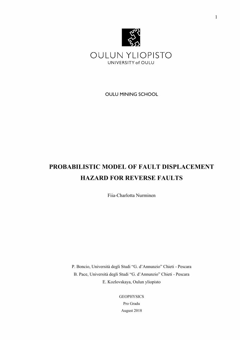
P. Boncio, Università degli Studi “G. d’Annunzio” Chieti - Pescara
B. Pace, Università degli Studi “G. d’Annunzio” Chieti - Pescara
E. Kozlovskaya, Oulun yliopisto
GEOPHYSICS
Pro Gradu
August 2018
2
ABSTRACT
FOR THESIS University of Oulu – Oulu Mining School Degree Programme (Bachelor's Thesis, Master’s Thesis) Major Subject (Licentiate Thesis)
Degree Programme in Physics
Author Thesis Supervisor
Nurminen, Fiia-Charlotta Kozlovskaya E., Professor, University of Oulu
Boncio, P., Professor, UNICH
Pace, B., Researcher, UNICH Title of Thesis
Probabilistic model of fault displacement hazard for reverse faults
Major Subject Type of Thesis Submission Date Number of Pages
Geophysics Master’s Thesis August 2018 83 p., 3 app.
Abstract
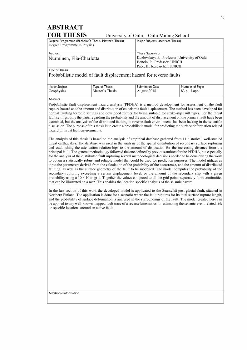
Probabilistic fault displacement hazard analysis (PFDHA) is a method development for assessment of the fault
rupture hazard and the amount and distribution of co-seismic fault displacement. The method has been developed for
normal faulting tectonic settings and developed further for being suitable for strike-slip fault types. For the thrust
fault settings, only the parts regarding the probability and the amount of displacement on the primary fault have been
examined, but the analysis of the distributed faulting in reverse fault environments has been lacking in the scientific
discussion. The purpose of this thesis is to create a probabilistic model for predicting the surface deformation related
hazard in thrust fault environments.
The analysis of this thesis is based on the analysis of empirical database gathered from 11 historical, well-studied
thrust earthquakes. The database was used in the analysis of the spatial distribution of secondary surface rupturing
and establishing the attenuation relationships to the amount of dislocation for the increasing distance from the
principal fault. The general methodology followed the one defined by previous authors for the PFDHA, but especially
for the analysis of the distributed fault rupturing several methodological decisions needed to be done during the work
to obtain a statistically robust and reliable model that could be used for prediction purposes. The model utilizes as
input the parameters derived from the calculation of the probability of the occurrence, and the amount of distributed
faulting, as well as the surface geometry of the fault to be modelled. The model computes the probability of the
secondary rupturing exceeding a certain displacement level, or the amount of the secondary slip with a given
probability using a 10 x 10 m grid. Together the values computed to all the grid points separately form continuities
that can be illustrated on a map. This enables the location specific analysis of the seismic hazard.
In the last section of this work the developed model is applicated to the Suasselkä post-glacial fault, situated in
Northern Finland. The application is done for a scenario where the fault ruptures for its total surface rupture length,
and the probability of surface deformation is analysed in the surroundings of the fault. The model created here can
be applied to any well-known mapped fault trace of a reverse kinematics for estimating the seismic event related risk
on specific locations around an active fault.
Additional Information

3
TIIVISTELMÄ
OPINNÄYTETYÖSTÄ Oulun yliopisto – Oulu Mining School Koulutusohjelma (kandidaatintyö, diplomityö) Pääaineopintojen ala (lisensiaatintyö)
Fysiikan tutkinto-ohjelma
Tekijä Työn ohjaaja yliopistolla
Fiia-Charlotta Nurminen Kozlovskaya E., professori, Oulun yliopisto
Boncio, P., professori, UNICH
Pace, B., tutkija, UNICH
Boncio, P., Professor, UNICH
Pace, B., Researcher, UNICH
Työn nimi
Probabilistic model of fault displacement hazard for reverse faults
Opintosuunta Työn laji Aika Sivumäärä
Geofysiikka Pro Gradu Elokuu 2018 83 s., 3 liite
Tiivistelmä
PFDHA-menetelmä (Probabilistic fault displacement hazard analysis) on kehitetty seismisiin siirrosvyöhykkeisiin
liittyvän riskin sekä seismisen siirtymän määrän ja jakauman arviointiin. Menetelmä on kehitetty normaalisiirroksille,
mutta sitä on kehitetty edelleen sivuttaissiirroksiin ja työntösiirroksiin sopivaksi. Työntösiiroksille on aiemmin
kehitetty vain pääsiirroksen siirtymän todennäköisyyttä ja määrää kuvaavat laskelmat, mutta sekundäärisiirrosten
analyysi on puuttunut tieteellisestä keskustelusta. Tämän pro gradu -tutkielman tarkoitus on luoda
todennäköisyyksiin perustuva ennustusmalli, jota voidaan käyttää mallintamaan maanpinnan muutoksiin liittyvää
riskiä työntösiirrosten ympäristössä.
Tämän tutkielman analyysi perustuu 11 historiallisen, hyvin tutkittuun työntösiirrosmaanjäristykseen. Näistä luotua
tietokantaa käytettiin sekundäärisiirrosten avaruudellisen jakauman arvioimiseen sekä sekundäärirepeämisen
vaimenemissuhteen analysoimiseen etäisyyden pääsiirrokseen kasvaessa. Käytetty menetelmä perustuu
pääpiirteissään perinteiseen PFDHA-menetelmään, mutta erityisesti näiden sekundäärisiirrosten analyysin osalta
menetelmää koskevia päätöksiä tuli tehdä työn edetessä, jotta lopputuloksena oli tilastollisesti pitävä ja uskottava
malli, jota voidaan käyttää riskin arvioinnissa. Malli käyttää syötteenään sekundäärisiirrosten tapahtumisesta ja
siirrosten suuruudesta johdettujen todennäköisyysfunktioiden muuttujia, sekä mallinnettavan siirroksen
pintageometriaa. Malli laskee sekundäärirepeämän todennäköisyyden ylittää annettu siirtymä tai määritetyllä
todennäköisyydellä tapahtuvan siirtymän suuruuden 10 x 10 m ruudukolla pääsiirroksen ympäristössä kullekin
ruudulle erikseen. Yhdessä näille ruuduille lasketuista arvoista muodostuu jatkumoja, joita voidaan kuvata kartalla.
Tämä antaa mahdollisuuden maanjäristykseen liittyvän seismisen riskin tarkkaan paikkakohtaiseen analyysiin.
Työn viimeisessä osassa kehitettyä mallia sovelletaan Pohjois-Suomessa sijaitsevaan Suasselän jääkauden jälkeiseen
työntösiirrokseen ja sen ympäristöön. Mallia sovelletaan skenaariolle, jossa siirros liikkuu koko pituudeltaan, ja
maanpinnan liikuntojen todennäköisyyttä mallinnetaan siirroksen ympäristössä. Tässä työssä kehitettyä mallia
voidaan soveltaa mille tahansa hyvin tunnetulle, aktiiviseksi määritellylle työntösiirrokselle siirroksen seismisen
riskin arvioimiseen tietyissä kohteissa siirroksen ympäristössä.
Muita tietoja

4
ACKNOWLEDGEMENTS
This MSc thesis is a result of highly inspiring research project conducted in the “G.
d’Annunzio” University of Chieti-Percara, Italy. I have not followed the most common
study path, and I want to express my gratitude to both the universities and all the people
involved. I would like to thank the University of Oulu and especially Oulu Mining School
and my thesis supervisor, professor Elena Kozlovskaya and this thesis reviewer,
researcher Kari Moisio for flexibility that allowed me to follow my interests of
specializing in earthquake geophysics and completing my studies in Italy. Equally, I
would like to express my gratitude to the ‘G. d’Annunzio’ University of Chieti-Pescara
and the department of DiSPuTer for giving me the opportunity to do the MSc thesis with
their professors and researchers. I am ever grateful to my thesis supervisors professor
Paolo Boncio and researcher Bruno Pace for creating highly motivating working
atmosphere and supporting my thesis process all the way. I appreciate their expertise on
earthquake geology and seismology, and I feel honoured for having worked in their
research group. I appreciate the support offered by Francesco Visini from INGV, whose
special knowledge in mathematical modelling was for great help. I would like to thank
also Alessandro Valentini for being my personal Matlab tutor. I want to thank also the
working group of the article published during the thesis process, Francesca Liberi and
Martina Caldarella for great collaboration with planning and executing the database.
Finally, I must express my very profound gratitude to my family and friends for the
support and encouragement throughout my years of study and through the process of
researching and writing this thesis.
Oulu, 13.08.2018 Fiia-Charlotta Nurminen
5
CONTENTS
ABSTRACT
TIIVISTELMÄ
ACKNOWLEDGEMENTS
ABBREVIATIONS
1 INTRODUCTION ......................................................................................................... 7
2 FAULT DISPLACEMENT HAZARD ........................................................................ 10
3 PFDHA METHODOLOGY ........................................................................................ 15
4 DATABASE ................................................................................................................ 21
5 ANALYSIS OF DISTRIBUTED FAULTING FOR THRUST FAULTS .................. 28
5.1 Occurrence of distributed faulting at various distances ........................................ 28
5.2 Attenuation relationships for displacement on distributed faults .......................... 32
5.2.1 Obtaining the normalization factors ............................................................ 33
5.2.2 Obtaining the dislocation distribution ......................................................... 39
5.2.3 Obtaining the probability distribution ......................................................... 49
6 APPLICATION OF THE MODEL ............................................................................. 53
6.1 Suasselkä post-glacial fault ................................................................................... 54
6.2 The scenario .......................................................................................................... 59
6.3 Probabilistic assessment for distributed faulting................................................... 60
7 DISCUSSION .............................................................................................................. 68
8 CONCLUSIONS .......................................................................................................... 71
REFERENCES ................................................................................................................ 73
APPENDICES:
Appendix 1. Structure of the database
Appendix 2. The vertical displacement levels with the 1% probability of exceedance
Appendix 3. The vertical displacement levels with the 2% probability of exceedance
6
ABBREVIATIONS
AD average displacement
DF distributed fault rupture (also called as secondary fault rupture)
Ga giga annum; billions of years
Mw moment magnitude
MD maximum displacement
PFDHA probabilistic fault displacement hazard analysis
PF principal fault rupture (also called as main fault rupture)
PG post-glacial
POE probability of exceedance
PSHA probabilistic seismic hazard analysis
SRL surface rupture length
VDL vertical displacements levels
WRZ width of the rupture zone
7
1 INTRODUCTION
Probabilistic fault displacement hazard analysis (PFDHA) is a method developed for
characterizing the expected fault rupture hazard and the amount and distribution of co-
seismic fault displacement (Coppersmith & Youngs, 2000). In a PFDHA, the rate of
displacement exceeding a certain amount during a seismic event is represented as function
of the fault slip rate (or the rate of earthquakes), the magnitude distribution, and the
distribution of the surface displacement at the site (Wells & Kulkarni, 2014). The PFDHA
is applied for design and placement of new critical structures (e.g. nuclear facilities) for
evaluation of the potential risk from fault displacement hazard to existing buildings and
structures once a new active fault is discovered, and for estimating the hazard for
infrastructures in cases where complete avoidance of the fault is not possible, like for
pipelines and roads (Moss & Ross, 2011). Furthermore, PFDHA provides a probability
of exceeding a given amount of fault displacement in a specified return period for the
displacement on and away from the primary fault trace. Thus, it is a key tool for hazard
analysis of any developed or developing seismic area crossed by active faults.
PFDHA follows the concept of probabilistic seismic hazard analysis (PSHA), the
development of which was started in late 1960s and has been used ever since for
evaluation of ground shaking hazards and establishing seismic design parameters
(Youngs et al., 2003 referring to Cornell, 1968 and Cornell, 1971). PSHA brings together
diverse types of data, such as the size and rates of earthquakes and attenuation of seismic
shaking, for mathematical estimation of the overall ground shaking related hazard (Baker,
2008). The development of PFDHA was begun by the working group of the Yucca
Mountain project, where they developed the analysis method for normal faulting,
extensional tectonic environments (Youngs et al., 2003). Later, the method has been
applied to strike-slip tectonic environments by several authors. However, thrust
environments have not been analysed in same detail as the other types of tectonic settings.
The previous studies regarding the probability of surface rupturing vs. magnitude (Moss
& Ross, 2011), and width of the rupture zones (WRZs) analysed in the initial section of
this research (see Boncio et al., 2018), have indicated that the characteristics of the thrust
earthquakes differ significantly from the ones of normal and strike-slip kinematics. Thus,
the generalized data of “all types of earthquakes” do not provide the best possible result
for predicting the damages caused by the seismic events of compressional kinematics.
For this reason, the scope of this MSc thesis is to develop a probabilistic model of fault
8
displacement hazard for thrust faults utilizing the empirical data of the historical
earthquakes on reverse tectonic settings.
The analysis of this work is based on the published material of eleven well-studied
historical thrust kinematics earthquakes occurred worldwide: 1971 San Fernando, CA,
USA; 1980 El Asnam, Algeria; 1983 Coalinga (Nuñez), CA, USA; 1986 Marryat Creek,
Australia; 1988 Tennant Creek, Australia; 1988 Spitak, Armenia; 1993 Killari, India;
1999 Chi-Chi, Taiwan; 2005 Kashmir, Pakistan; 2008 Wenchuan, China; and 2014
Nagano, Japan. These events were chosen because of the availability of detailed rupture
maps and displacement data, along principal and secondary fault ruptures during the
earthquakes. The events were analysed by collecting slip parameter data along the
principal fault trace as well as of the distributed surface ruptures further away from the
principal surface rupture fault. The created database was then used for the analysis of the
probability and spatial distribution of the secondary faulting during thrust earthquakes.
The database, as well as some parts of the work done during this thesis regarding the
distribution of the secondary surface rupturing, have been published with the research
group as an article entitled ‘Width of surface rupture zone for thrust earthquakes:
implications for earthquake fault zoning’ (Boncio et al., 2018), in which I was pleased to
be a co-author. The database is available as a supplementary material of the paper. The
scope of the research paper was limited to the analysis of the distribution of secondary
faulting, thus the database published along the paper is incomplete for analysing the
parameters of principal fault rupturing. Thus, the database has been completed for the
purposes of estimating the regressions of the amount of displacement on secondary faults,
which required the normalization parameters from the displacement along the principal
fault trace.
This work takes the traditional PFDHA a step further including the new regressions for
distributed rupturing for thrust faults into the prediction model. The created model is
applied to an active fault that is considered to be capable of producing a surface rupturing
earthquake in the future. The chosen fault is the Suasselkä post-glacial fault situated in
Lapland, Northern Finland. The seismicity of the Suasselkä fault system has been studied
by various authors, but there is no clear consensus of seismic activity of the fault. Based
on the work of Afonin et al. (2017), the Suasselkä fault can be considered as a potential
source of earthquake related hazard and thus a reasonable zone of applicating the created
model. The area around the fault is sparsely populated, but there are multiple other
9
activities in the near vicinity of the fault trace, including an operative gold mine and a
skiing centre, which is one of the most active recreational areas in Finnish Lapland. In
general, the whole Fennoscandian Shield is a zone of intraplate seismicity and low
seismic risk. This does not mean that there is no risk present, but it explains why there is
a little previous work done considering the seismic hazard in the area. The applicability
of the model to these intraplate and low seismic risk areas is important also in cases when
looking for the placement for operations highly sensitive to the tectonic movements.
In this thesis, I will first define the basic concepts related to this type of hazard assessment
in Chapter 2: Fault Displacement Hazard. Then, in Chapter 3: PFDHA methodology, the
reader will be introduced to the used methodology in the way it has been developed by
the previous authors. The analysis done in this work is strongly based on the empirical
analysis of the historical thrust earthquakes and the parameters obtained from the created
database. This part is explained in detail in Chapter 4: Database. In the following, Chapter
5: Analysis of Distributed Faulting for Thrust Faults describes the methodological
improvements for the PFDHA method developed in this work for the model to be more
precisely applicable to reverse faulting environments. Finally, the created model is
applicated to an existing fault environment, which is described in detail in Chapter 6:
Application of the model.
This Master’s Thesis was done in Oulu Mining School of the University of Oulu, Finland
in close collaboration with the ‘Gabriele d’Annunzio’ University of Chieti-Pescara, Italy.
10
2 FAULT DISPLACEMENT HAZARD
Fault displacement hazard is a local seismic hazard rising from the potential co-seismic
surface rupturing due to slip along the seismogenic fault. This sort of surface deformation
is likely to cause significant damage to the infrastructure situated on or near a ruptured
area. Understanding the hazard is crucial on the general safety in the vicinity of tectonic
faults considered active and capable of producing earthquakes. The potential extent of
hazard is estimated when the geological parameters of the fault, such as surface rupture
length (SRL), slip rate, maximum expected magnitude and co-seismic displacement are
known. The more parameters, i.e. the more information, is added on the hazard analysis,
the more accurate the estimation of the potential hazard gets.
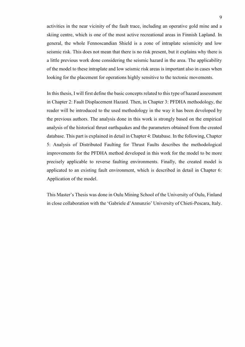
There are three main types of faults along which the tectonic movement takes place. The
thematic illustrations are shown in Figure 1 below. The tectonic setting can be either of
lateral movement, when the blocks are sliding past each other (b), or dip slip movement,
where the blocks move vertically amongst other: the setting of extensional movement is
called normal dip-slip fault (a) and the setting where the principal force is contracting is
called reverse or thrust fault (c). This work concentrates on thrust fault setting, where the
hanging wall slides on top of the footwall. Subduction zone thrust earthquakes were not
included in this study, as they produce pattern and style of deformation that is beyond the
scope of this work. The movement can also be a combination of two movements, the
lateral and one of the dip slip movements, also known as an oblique slip. The events of
oblique slipping with remarkable reverse slip factor were also included in the analysis.
Figure 1 Schematic figures of three main types of faulting: (a) normal fault, (b) strike-
slip fault an (c) reverse (or thrust) fault. (modified from Paananen, 1987)
11
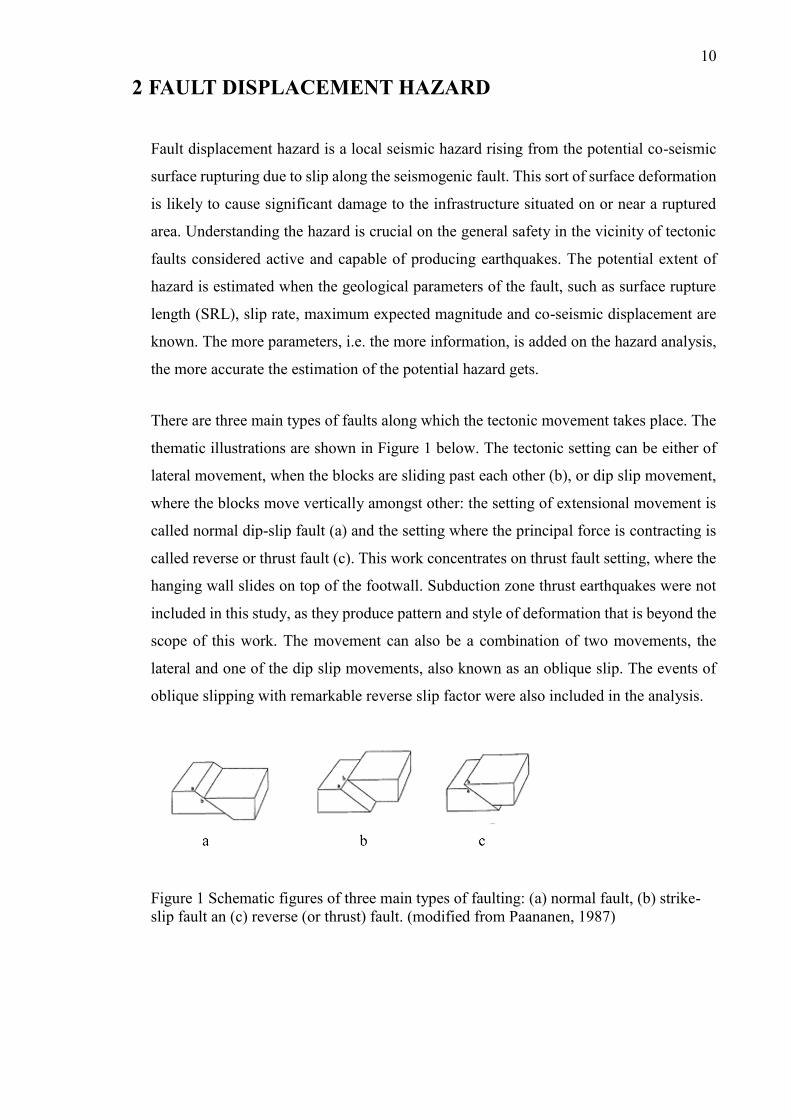
Figure 2 Building tilted due to an uplift of 4 m after thrust faulting during the 1999 Chi
Chi earthquake (photo: Kelson et al., 2003; sketch: Paananen, 1987)
Thrust fault can rupture up to the surface or remain blind. A blind thrust fault does not
break up to the ground surface but remains “buried” under the uppermost layers of the
crust. These blind events can also be relatively strong on their magnitude, and it is
likewise possible that an earthquake of large magnitude produces a surface rupture
remarkably shorter than the whole length of the fault. In some cases when the main fault
plane does not break to the surface, the coseismic displacement may still produce notable
anticlinal deformation on the ground surface. (Lettis et al., 1997) Thus, the damage to the
surface or near-surface infrastructure caused by an earthquake on a fault of reverse
tectonics depends largely on the fault breaking up to the surface or remaining buried. In
this work I concentrate only on the events associated with the evident surface rupturing.
The photo in Figure 2 above, taken after 1999 Chi Chi earthquake in Taiwan, shows an
example of damage caused by a thrust earthquake rupturing all the way to the surface. It
illustrates the different scales of dislocation on the two sides of the principal fault: the
structure on left seems rather unharmed due to its location on the footwall of the fault,
whereas the tilted building on the right lies on the hanging wall that has risen upwards
during the earthquake.
12
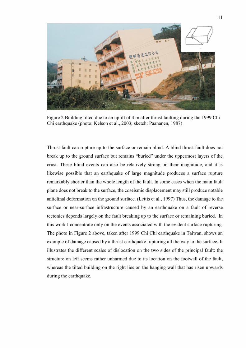
Figure 3 Examples showing generalized surface deformation and inferred subsurface
fault geometries in various schematic structural models of surface rupturing caused by
thrust earthquakes (Kelson et al., 2001)
Figure 3 illustrates the thematic structure of the surface damage in some of the typical
scenarios of thrust fault earthquakes producing surface rupturing. The width of the
damaged area as well as the magnitude of the surface damage caused by a tectonic event
depends largely on the geological structure below the surface. Thrust fault often creates
an uplift that bends the surface level, hanging wall rising on top of the footwall. The
dimension of the bending depends on the dip angle of the fault, steeply dipping fault
13
causing higher uplift compared to milder dipping fault. Changes in the dip angle along
the fault plane can cause bending on the hanging wall also further from the point where
the main fault plane breaks the ground surface. Splitting into various fault planes
increases the width of the rupture zone on the ground surface, as the movement is
forwarded further among the fault planes other than the principal one. The fault scarp can
remain clear and visible when the material around the fault trace is hard (bedrock), but
those fault scarps are likely to collapse within time. On areas of soft or loose material on
the surface, no clear scarp is visible.
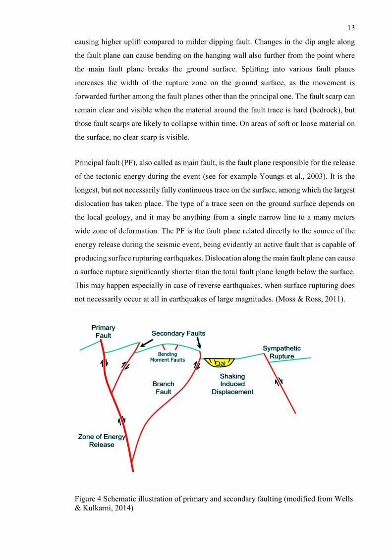
Principal fault (PF), also called as main fault, is the fault plane responsible for the release
of the tectonic energy during the event (see for example Youngs et al., 2003). It is the
longest, but not necessarily fully continuous trace on the surface, among which the largest
dislocation has taken place. The type of a trace seen on the ground surface depends on
the local geology, and it may be anything from a single narrow line to a many meters
wide zone of deformation. The PF is the fault plane related directly to the source of the
energy release during the seismic event, being evidently an active fault that is capable of
producing surface rupturing earthquakes. Dislocation along the main fault plane can cause
a surface rupture significantly shorter than the total fault plane length below the surface.
This may happen especially in case of reverse earthquakes, when surface rupturing does
not necessarily occur at all in earthquakes of large magnitudes. (Moss & Ross, 2011).
Figure 4 Schematic illustration of primary and secondary faulting (modified from Wells
& Kulkarni, 2014)
14
Distributed faulting (DF), also called as secondary faulting, means the displacement along
faults, shears, or fractures other than the one causing the seismic event. Distributed
faulting is not responsible for the earthquake event, but the dislocation is a response to
the movement on the main fault, see Figure 4 above. Distributed faults are found mainly
near the principal fault, but depending on the geological setting, they can reach also
distances of several kilometres. A distributed fault rupture may be a distinct fault other
than the one regarded as a PF, but it can also be a splay off from the principal fault trace.
Especially in the close vicinity of the main fault the distributed faulting happens as a result
to the burst of the seismic energy, which opens faulting on new planes of local crustal
weaknesses, which has not necessarily existed previously. However, the release of
tectonic energy may reactivate slip along existing fault planes, and this type of distributed
faulting can take place also remarkably far from the principal fault. Distributed faulting
along these pre-existing fault planes can be categorized as displacement along
sympathetic fault ruptures. Unlike principal faults, distributed faults do not necessarily
need to be capable of producing earthquakes on their own, but they might as well be the
ones regarded as active and capable ones. Thus, the kinematics and orientation of the
secondary ruptures might sometimes differ largely from those of the principal fault of the
event, though most often they are parallel or sub-parallel to the PF. (See e.g. Youngs et
al., 2003 and Petersen et al., 2011).
15
3 PFDHA METHODOLOGY
Probabilistic fault displacement hazard analysis (PFDHA) was developed at the turn of
the century for the purposes of establishing a high-level nuclear waste repository in
normal fault zone in Nevada, USA; see Youngs et al., 2003. Before the development of
PFDHA, the fault displacement hazard was handled mainly by avoidance, and for those
facilities that must pass the fault areas, like pipelines and roads, the approach has
traditionally been either deterministic hazard evaluation, or acceptance of the risk. Since
a facility like the high-level nuclear waste repository is very sensitive to any
displacement, the working group of Yucca Mountain repository project put significant
effort on the development of the PFDHA method. Youngs et al. (2003) provide two
approaches to the hazard analysis: the earthquake approach and the displacement
approach. The procedure of the earthquake approach follows the methodology used for
the traditional probabilistic seismic hazard analysis (PSHA), with the exception of the
ground motion attenuation function replaced by a fault displacement attenuation function.
The displacement approach is based on the characteristics of fault displacement or
geological features observed at the site and the hazard is quantified on that basis.
Commonly the PFHDA is performed using the earthquake approach, which is coherent
with the PSHA methodology by the source identification and characterization of the rate
and size distribution of earthquakes, as well as the distance distribution. Applying the
PFDHA adds, however, information on the rupture geometry and computes the
conditional probability of exceeding a certain displacement using a displacement
attenuation relationship, unlike in PSHA. The key difference between these methods lies
in the finite probability of no slip will occur, which is not considered in ground shaking
analysis. The probability distributions are brought together to develop a displacement
hazard curve that expresses the displacement at a point to the rate that it is exceeded.
(Youngs et al., 2003)
The traditional PFDHA consists of four key parts, which are: 1) the characterization of
the earthquake magnitude, 2) the rate of occurrence of earthquakes on the fault, 3) the
occurrence of a rupture along the fault given that a magnitude M earthquake occurs, and
4) the expected amount and distribution of fault displacement at the site of interest (Wells
& Kulkarni 2014). For fault displacement analysis, the distinction is needed between the
primary displacement along the distinct fault trace and the distributed ruptures. In the
model developed for the Yucca Mountain project, however, only the normal faulting
16
environments were considered, and the model has been applied to other fault types by
other authors. The method was developed further by Petersen et al. (2011) and Moss &
Ross (2011) so that the methodology would be applicable also for the strike-slip and
reverse faulting mechanisms, respectively.
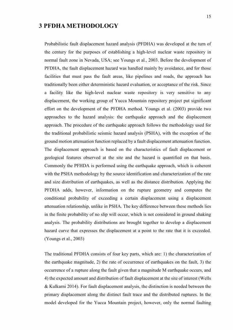
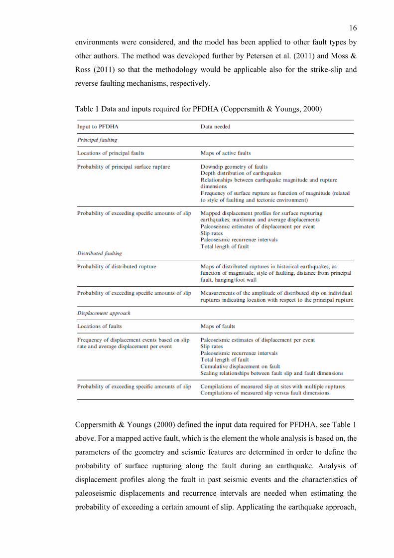
Table 1 Data and inputs required for PFDHA (Coppersmith & Youngs, 2000)
Coppersmith & Youngs (2000) defined the input data required for PFDHA, see Table 1
above. For a mapped active fault, which is the element the whole analysis is based on, the
parameters of the geometry and seismic features are determined in order to define the
probability of surface rupturing along the fault during an earthquake. Analysis of
displacement profiles along the fault in past seismic events and the characteristics of
paleoseismic displacements and recurrence intervals are needed when estimating the
probability of exceeding a certain amount of slip. Applicating the earthquake approach,
17
the distributed faulting during historical events are mapped and analysed as function of
magnitude, a style of faulting and distance from principal faulting, indicating the side in
respect to the principal fault. This is done for estimating the probability of distributed
faulting during a future seismic event. In addition, for the analysis of the amount of
dislocation on distributed faulting, the measurement of the amplitude of distributed slip
is needed.
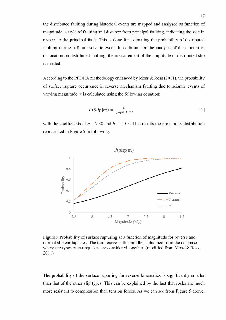
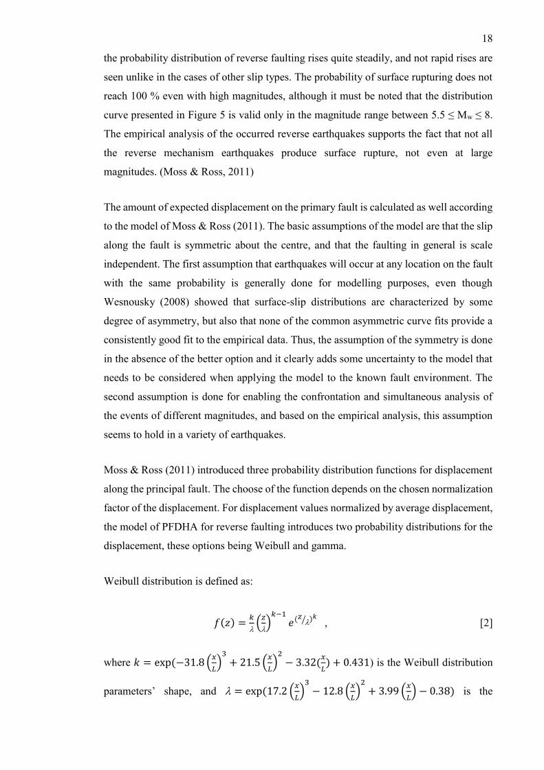
According to the PFDHA methodology enhanced by Moss & Ross (2011), the probability
of surface rupture occurrence in reverse mechanism faulting due to seismic events of
varying magnitude m is calculated using the following equation:
𝑃(𝑆𝑙𝑖𝑝|𝑚) = 1
1+𝑒𝑎+𝑏∗𝑚, [1]
with the coefficients of a = 7.30 and b = -1.03. This results the probability distribution
represented in Figure 5 in following.
Figure 5 Probability of surface rupturing as a function of magnitude for reverse and
normal slip earthquakes. The third curve in the middle is obtained from the database
where are types of earthquakes are considered together. (modified from Moss & Ross,
2011)
The probability of the surface rupturing for reverse kinematics is significantly smaller
than that of the other slip types. This can be explained by the fact that rocks are much
more resistant to compression than tension forces. As we can see from Figure 5 above,
18
the probability distribution of reverse faulting rises quite steadily, and not rapid rises are
seen unlike in the cases of other slip types. The probability of surface rupturing does not
reach 100 % even with high magnitudes, although it must be noted that the distribution
curve presented in Figure 5 is valid only in the magnitude range between 5.5 ≤ Mw ≤ 8.
The empirical analysis of the occurred reverse earthquakes supports the fact that not all
the reverse mechanism earthquakes produce surface rupture, not even at large
magnitudes. (Moss & Ross, 2011)
The amount of expected displacement on the primary fault is calculated as well according
to the model of Moss & Ross (2011). The basic assumptions of the model are that the slip
along the fault is symmetric about the centre, and that the faulting in general is scale
independent. The first assumption that earthquakes will occur at any location on the fault
with the same probability is generally done for modelling purposes, even though
Wesnousky (2008) showed that surface-slip distributions are characterized by some
degree of asymmetry, but also that none of the common asymmetric curve fits provide a
consistently good fit to the empirical data. Thus, the assumption of the symmetry is done
in the absence of the better option and it clearly adds some uncertainty to the model that
needs to be considered when applying the model to the known fault environment. The
second assumption is done for enabling the confrontation and simultaneous analysis of
the events of different magnitudes, and based on the empirical analysis, this assumption
seems to hold in a variety of earthquakes.
Moss & Ross (2011) introduced three probability distribution functions for displacement
along the principal fault. The choose of the function depends on the chosen normalization
factor of the displacement. For displacement values normalized by average displacement,
the model of PFDHA for reverse faulting introduces two probability distributions for the
displacement, these options being Weibull and gamma.
Weibull distribution is defined as:
𝑓(𝑧) =𝑘
(
𝑧
)
𝑘−1
𝑒(𝑧⁄ )𝑘
, [2]
where 𝑘 = exp (−31.8 (𝑥
𝐿)
3
+ 21.5 (𝑥
𝐿)
2
− 3.32(𝑥
𝐿) + 0.431) is the Weibull distribution
parameters’ shape, and = exp (17.2 (𝑥
𝐿)
3
− 12.8 (𝑥
𝐿)
2
+ 3.99 (𝑥
𝐿) − 0.38) is the
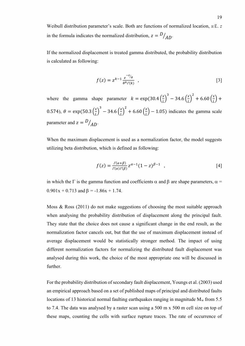
19
Weibull distribution parameter’s scale. Both are functions of normalized location, x/L. z
in the formula indicates the normalized distribution, 𝑧 = 𝐷𝐴𝐷⁄ .
If the normalized displacement is treated gamma distributed, the probability distribution
is calculated as following:
𝑓(𝑧) = 𝑧𝑘−1 𝑒−𝑧
𝜃⁄
𝜃𝑘(𝑘) , [3]
where the gamma shape parameter 𝑘 = exp (30.4 (𝑥
𝐿)
3
− 34.6 (𝑥
𝐿)
2
+ 6.60 (𝑥
𝐿) +
0.574), 𝜃 = exp (50.3 (𝑥
𝐿)
3
− 34.6 (𝑥
𝐿)
2
+ 6.60 (𝑥
𝐿) − 1.05) indicates the gamma scale
parameter and 𝑧 = 𝐷𝐴𝐷⁄ .
When the maximum displacement is used as a normalization factor, the model suggests
utilizing beta distribution, which is defined as following:
𝑓(𝑧) =(𝛼+𝛽)
(𝛼)(𝛽)𝑧𝛼−1(1 − 𝑧)𝛽−1 , [4]
in which the is the gamma function and coefficients and are shape parameters, =
0.901x + 0.713 and = -1.86x + 1.74.
Moss & Ross (2011) do not make suggestions of choosing the most suitable approach
when analysing the probability distribution of displacement along the principal fault.
They state that the choice does not cause a significant change in the end result, as the
normalization factor cancels out, but that the use of maximum displacement instead of
average displacement would be statistically stronger method. The impact of using
different normalization factors for normalizing the distributed fault displacement was
analysed during this work, the choice of the most appropriate one will be discussed in
further.
For the probability distribution of secondary fault displacement, Youngs et al. (2003) used
an empirical approach based on a set of published maps of principal and distributed faults
locations of 13 historical normal faulting earthquakes ranging in magnitude Mw from 5.5
to 7.4. The data was analysed by a raster scan using a 500 m x 500 m cell size on top of
these maps, counting the cells with surface rupture traces. The rate of occurrence of

20
distributed rupturing was calculated dividing the number of cells containing distributed
rupturing by the total number of cells within the faulting area. The conditional probability
of distributed rupturing occurring at a point was then computed using the logistic
regression model because of the binary nature of the surface rupture outcome. Petersen et
al. (2011) followed the methodology of Youngs et al. (2003), digitizing the distributed
faulting of 9 strike-slip earthquakes up to 12 kilometres from the principal fault using five
different cell sizes ranging from 25 to 200 m on a side. In the database of Petersen et al.,
they excluded the sympathetic faulting, that most of the distributed faulting is beyond 2-
km distances, but the authors recognized the fault rupture hazard caused by these
triggered faults. They analysed the potential for DF displacement as a function of distance
from the PF. As they used various cell sizes, expectedly as the cell size decreases, there
is a corresponding decrease also in the probability of rupturing. Moss & Ross (2011)
concentrated their work on the analysis of the principal fault rupture, determining the
distribution functions for reverse slip data using the dataset of Lettis et al. (1997)
containing events both with and without surface rupture, complemented with six more
recent events, five of which with surface rupturing. The probability distribution for off-
fault rupturing in reverse slip earthquakes was not defined. This work emphasises on
including the distributed faulting related surface rupture hazard into PFDHA for reverse
slip faults. The applied methodology used for analysing the occurrence of the secondary
fault rupturing differs from the one used by the research groups mentioned earlier, adding
some accuracy to the analysis. This more detailed approach for obtaining the database is
explained in detail in the following chapter.

21
4 DATABASE
The database was assembled by gathering the data from the chosen 11 events to a uniform
table. Building up the database was done in collaboration with Martina Caldarella, who
had studied some of the considered earthquakes already for her MSc thesis, which
concentrated on the fault zones with distributed faulting on these events (Caldarella,
2016). Parts of this work including the database on the parts considering the distributed
fault rupturing were published in the research paper of Boncio et al. (2018), along which
the database is available as a supplementary material (Table S1). The published database
was limited to the scope of the research paper, i.e. the distributed rupturing. Thus, it
includes all the secondary rupturing, but lacks in information of principal rupturing in
areas with no associated secondary faulting. The published database was completed later
regarding the earthquakes that were studied systematically to the full extent of the
principal fault rupture, these being the earthquakes of 1971 San Fernando, 1983 Coalinga,
1986 Marryat Creek, 1988 Tennant Creek. The data of 2008 Wenchuan earthquake was
also completed by its principal fault rupturing. In addition, some arbitrary values of 1 cm
horizontal dislocation indicating open fissures were eliminated from the published
version of the database as they would have interrupted the analysis of the amount of the
dislocation. Similarly, those few cases of the secondary fault dislocation values exceeding
the corresponding maximum along the principal fault were excluded from the database.
The database was compiled by GIS-georeferencing the maps and dislocation
measurements published by the authors that have studied the surface deformation directly
after the earthquake event. Hence, the measurements are mainly of tectonic displacement,
but they may contain also some afterslip movement as the measurements were done some
hours to some days after the event. In those rare cases where the displacement was
measured more than once in the same location, only the most recent measurement after
the earthquake was considered for the database. The accuracy of the measurements
depends largely on the scale of the original maps and on the level of reported details. Only
detailed maps with clear indication of the location were considered for this work. When
analysing the maps, the principal surface rupture fault trace was interpreted to be the one
with the largest displacement, longest continuity, and coincidence or nearly coincidence
with major tectonic or geomorphologic features, such as the trace of the fault mapped
before the earthquake on geologic maps. In some cases, interpretation of the trace of the
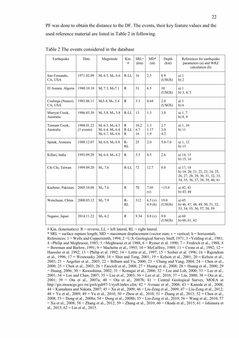
22
PF was done to obtain the distance to the DF. The events, their key feature values and the
used reference material are listed in Table 2 in following.
Table 2 The events considered in the database
Earthquake Date Magnitude Kin.
# SRL*
(km) MD*
(m) Depth
(km) References for earthquake
parameters (a) and WRZ
calculation (b)
San Fernando,
CA, USA 1971.02.09 Ms 6.5, Mw 6.6 R-LL 16 2.5 8.9
(USGS) a) 1
b) 2
El Asnam, Algeria 1980.10.10 Ms 7.3, Mw7.1 R 31 6.5 10
(USGS) a) 1
b) 3, 4, 5
Coalinga (Nunez),
CA, USA 1983.06.11 Ms5.4, Mw 5.4 R 3.3 0.64 2.0
(USGS) a) 1
b) 6
Marryat Creek,
Australia 1986.03.30 Ms 5.8, Mw 5.8 R-LL 13 1.3 3.0 a) 1, 7
b) 8, 9
Tennant Creek,
Australia 1988.01.22
(3 events) Ms 6.3, Mw 6.3
Ms 6.4, Mw 6.4
Ms 6.7, Mw 6.6
R
R-LL
R
10.2
6.7
16
1.3
1.17
1.9
2.7
3.0
4.2
a) 1, 10
b) 11
Spitak, Armenia 1988.12.07 Ms 6.8, Mw 6.8 R-
RL 25 2.0 5.0-7.0 a) 1, 12
b) 13
Killari, India 1993.09.29 Ms 6.4, Mw 6.2 R 5.5 0.5 2.6 a) 14, 15
b) 15, 16
Chi Chi, Taiwan 1999.09.20 Mw 7.6 R-LL 72 12.7 8.0 a) 17, 18
b) 19, 20, 21, 22, 23, 24, 25,
26, 27, 28, 29, 30, 31, 32, 33,
34, 35, 36, 37, 38, 39, 40, 41
Kashmir, Pakistan 2005.10.08 Mw 7.6 R 70 7.05
(v) <15.0 a) 42, 43
b) 43, 44
Wenchuan, China 2008.05.12 Mw 7.9 R-
RL 312 6.5 (v)
4.9 (h) 19.0
(USGS) a) 45
b) 46, 47, 48, 49, 50, 51, 52,
53, 54, 55, 56, 57, 58, 59
Nagano, Japan 2014.11.22 Mw 6.2 R 9.34 0.8 (v) 9.0
(USGS)
a) 60
b) 60, 61, 62
# Kin. (kinematics): R = reverse, LL = left lateral, RL = right lateral.
* SRL = surface rupture length; MD = maximum displacement (vector sum; v = vertical; h = horizontal).
References: 1 = Wells and Coppersmith, 1994; 2 =U.S. Geological Survey Staff, 1971; 3 =Yelding et al., 1981;
4 =Philip and Meghraoui, 1983; 5 =Meghraoui et al 1988; 6 = Rymer et al. 1990; 7 = Fredrich et al., 1988; 8
= Bowman and Barlow, 1991; 9 = Machette et al., 1993; 10 = McCaffrey, 1989; 11 = Crone et al., 1992; 12 =
Haessler et al. 1992; 13 = Philip et al. 1992; 14 = Lettis et al., 1997; 15 = Seeber et al. 1996; 16 = Rajendran
et al., 1996; 17 = Wesnousky 2008; 18 = Shin and Teng, 2001; 19 = Kelson et al., 2001; 20 = Kelson et al.,
2003; 21 = Angelier et al., 2003; 22 = Bilham and Yu, 2000; 23 = Chang and Yang, 2004; 24 = Chen et al.,
2000; 25 = Chen et al., 2003; 26 = Faccioli et al., 2008; 27 = Huang et al., 2008; 28 = Huang et al., 2000; 29
= Huang, 2006; 30 = Kawashima, 2002; 31 = Konagai et al., 2006; 32 = Lee and Loh, 2000; 33 = Lee et al.,
2001; 34 = Lee and Chan, 2007; 35 = Lee et al., 2003; 36 = Lee et al., 2010; 37 = Lin, 2000; 38 = Ota et al.,
2001; 39 = Ota et al., 2007a; 40 = Ota et al., 2007b; 41 = Central Geological Survey, MOEA at
http://gis.moeacgs.gov.tw/gwh/gsb97-1/sys8/index.cfm; 42 = Avouac et al., 2006; 43 = Kaneda et al., 2008;
44 = Kumahara and Nakata, 2007; 45 = Xu et al., 2009; 46 = Liu-Zeng et al., 2009; 47 = Liu-Zeng et al., 2012;
48 = Yu et al., 2009; 49 = Yu et al., 2010; 50 = Zhou et al., 2010; 51 = Zhang et al., 2013; 52 = Chen et al.,
2008; 53 = Dong et al., 2008a; 54 = Dong et al., 2008b; 55 = Liu-Zeng et al., 2010; 56 = Wang et al., 2010; 57
= Xu et al., 2008; 58 = Zhang et al., 2012; 59 = Zhang et al., 2010; 60 = Okada et al., 2015; 61 = Ishimura et
al., 2015; 62 = Lin et al., 2015.
23
The database was created by gathering the data of the displacement (horizontal, vertical,
strike-slip and total net displacement, if available) on the principal fault rupture and
coordinates of the referred measurement points on the PF having associated distributed
ruptures. For the principal fault, net displacement can be calculated as a vector sum of
vertical, horizontal and strike-slip displacements when reported in the same location, or
by using the basic geometry when the fault dip angle and some of these vectors are known.
However, the secondary faults can have different orientations, so calculating the net slip
using the geometry and an assumption of the dip angle cannot be equally justified. In very
few cases all the vectors of the movement on the secondary rupture were provided, thus
using the net displacement was tested calculating vector sum of the movement assuming
the vectors with not reported length to be zero. The distributed rupturing was reported
distinguishing between the ones on hanging wall and on footwall. The perpendicular
distances between the PF and the secondary fault ruptures were gathered in every 200 m
for the long secondary structures. When the length of the secondary surface rupture was
between 200 and 400 m, the distance was measured from the end points and the midpoint.
In cases when the secondary fault trace was shorter than 200 m, the distance measurement
was taken only from the midpoint of the trace. When dislocation information was
associated to the distributed fault, these locations were prioritized when choosing the
measurement points, and the overall measurement logic was adjusted accordingly
avoiding over measuring any of the faults. For determining the perpendicular to the PF,
the strike direction was approximated along the fault segments. The direction of the
measurement was taken in respect to these approximated fault traces, but the distance was
always measured between the real fault traces. The WRZ was measured as the maximum
width of the ruptured zone in every measurement point, on hanging wall and footwall
separately. Thus, the methodology for examining the distribution of secondary faulting
used in this work differs significantly from the grid-based approach used by Youngs et
al. (2003) and Petersen et al. (2011). The results of their analyses could not be confronted
regardless, due to the features of the different faulting types, and the methodology
developed here seems to rather increase the accuracy of the analysis rather than decrease
it.
All the georeferenced maps with the drawn measurement lines used for creating the
database can be found as a supplementary material of the article of Boncio et al. (2018).
The measurement logic and the special case of the Sylmar segment of the San Fernando
fault is shown as an example in Figure 7. In San Fernando a lot of distributed surface
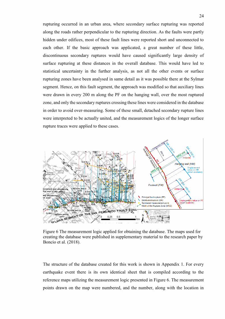
24
rupturing occurred in an urban area, where secondary surface rupturing was reported
along the roads rather perpendicular to the rupturing direction. As the faults were partly
hidden under edifices, most of these fault lines were reported short and unconnected to
each other. If the basic approach was applicated, a great number of these little,
discontinuous secondary ruptures would have caused significantly large density of
surface rupturing at these distances in the overall database. This would have led to
statistical uncertainty in the further analysis, as not all the other events or surface
rupturing zones have been analysed in same detail as it was possible there at the Sylmar
segment. Hence, on this fault segment, the approach was modified so that auxiliary lines
were drawn in every 200 m along the PF on the hanging wall, over the most ruptured
zone, and only the secondary ruptures crossing these lines were considered in the database
in order to avoid over-measuring. Some of these small, detached secondary rupture lines
were interpreted to be actually united, and the measurement logics of the longer surface
rupture traces were applied to these cases.
The structure of the database created for this work is shown in Appendix 1. For every
earthquake event there is its own identical sheet that is compiled according to the
reference maps utilizing the measurement logic presented in Figure 6. The measurement
points drawn on the map were numbered, and the number, along with the location in
Figure 6 The measurement logic applied for obtaining the database. The maps used for
creating the database were published in supplementary material to the research paper by
Boncio et al. (2018).
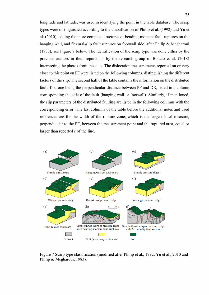
25
longitude and latitude, was used in identifying the point in the table database. The scarp
types were distinguished according to the classification of Philip et al. (1992) and Yu et
al. (2010), adding the more complex structures of bending-moment fault ruptures on the
hanging wall, and flexural-slip fault ruptures on footwall side, after Philip & Megharoui
(1983), see Figure 7 below. The identification of the scarp type was done either by the
previous authors in their reports, or by the research group of Boncio et al. (2018)
interpreting the photos from the sites. The dislocation measurements reported on or very
close to this point on PF were listed on the following columns, distinguishing the different
factors of the slip. The second half of the table contains the information on the distributed
fault, first one being the perpendicular distance between PF and DR, listed in a column
corresponding the side of the fault (hanging wall or footwall). Similarly, if mentioned,
the slip parameters of the distributed faulting are listed in the following columns with the
corresponding error. The last columns of the table before the additional notes and used
references are for the width of the rupture zone, which is the largest local measure,
perpendicular to the PF, between the measurement point and the ruptured area, equal or
larger than reported r of the line.
Figure 7 Scarp type classification (modified after Philip et al., 1992; Yu et al., 2010 and
Philip & Megharoui, 1983).
26
All the distributed fault ruptures reported were taken into consideration, except some of
those from Sylmar segment of the 1971 San Fernando event for the reasons explained
before, and the Beni Rached rupture zone of the 1981 El Asnam earthquake. The Beni
Rached rupture zone of the El Asnam event was not considered in the database, as
according to the previous authors, it should be interpreted either as a very large
gravitational sliding, or a surface response of an unconstrained tectonic fault responsible
for the 1954 M 6.7 earthquake (Yelding et al., 1981; Philip & Megharoui, 1983). Due to
the large uncertainty regarding its origin, this fault segment was left out from the database.
In addition to the classification demonstrated in Figure 7, the DFs rather unconnected to
the PF were classified as sympathetic fault ruptures, despite their scarp type. These are
distributed faulting on pre-existing faults especially in rather large distance (> 2 km) from
the PF, triggered by the release of the seismic energy on the main fault. Sympathetic
secondary rupturing was noted in San Fernando, El Asnam, 1988 Tennant Creek and the
1999 Chi Chi earthquake events.
The analysis of the distribution of the secondary fault dislocation was done for data
grouped for sub-databases according to the data type for finding the most adequate
approach. The data was divided by the side respect to the PF (hanging wall / footwall),
by the complexity of the scarp type (‘simple’ / ‘all’), and finally by the slip type
considered (vertical / net). The complexity of the data means in this case that the
secondary faults associated with complex local geology were either included (‘all’) or
excluded (‘simple’) from the data. These complex type secondary faults include bending-
moment and flexural slip, and so called sympathetic faults, which means a slip occurred
further away, on pre-existing faults triggered by the most recent event. The data divided
in each category was analysed separately, the corresponding pairs of databases on
footwall and hanging wall to be united later for the overall analysis of a chosen scenario.
Some secondary faults on the hanging wall of the earthquakes considered in this work
acted like normal faults near the surface. Thus, their vertical slip was reported negative
in the initial database indicating the opposite direction to the vertical reverse slip on the
principal fault. These values are excluded in analyses where pure vertical slip is
considered and included as absolute values in sub-databases indicated as ‘absolute’. The
logic tree illustrating the division into the sub-databases is shown in Figure 8.
27
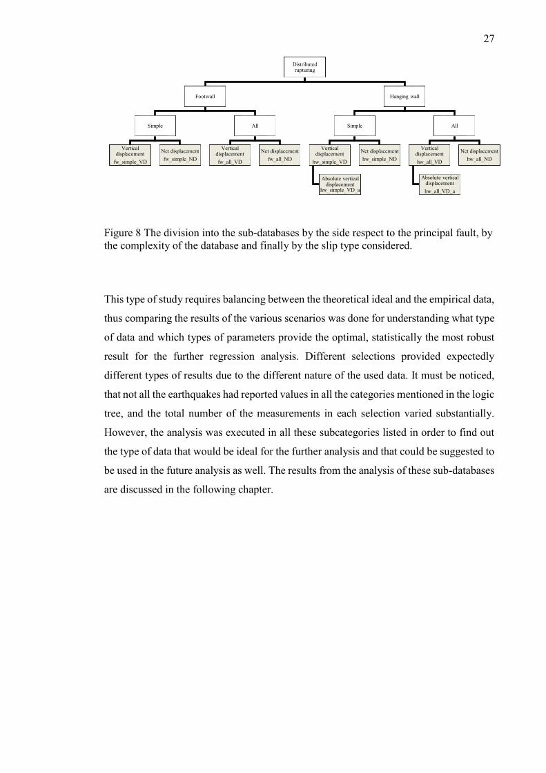
Figure 8 The division into the sub-databases by the side respect to the principal fault, by
the complexity of the database and finally by the slip type considered.
This type of study requires balancing between the theoretical ideal and the empirical data,
thus comparing the results of the various scenarios was done for understanding what type
of data and which types of parameters provide the optimal, statistically the most robust
result for the further regression analysis. Different selections provided expectedly
different types of results due to the different nature of the used data. It must be noticed,
that not all the earthquakes had reported values in all the categories mentioned in the logic
tree, and the total number of the measurements in each selection varied substantially.
However, the analysis was executed in all these subcategories listed in order to find out
the type of data that would be ideal for the further analysis and that could be suggested to
be used in the future analysis as well. The results from the analysis of these sub-databases
are discussed in the following chapter.
Distributed rupturing
Footwall
Simple
Vertical displacement
fw_simple_VD
Net displacement
fw_simple_ND
All
Vertical displacement
fw_all_VD
Net displacement
fw_all_ND
Hanging wall
Simple
Vertical displacement
hw_simple_VD
Absolute vertical displacement
hw_simple_VD_a
Net displacement
hw_simple_ND
All
Vertical displacement
hw_all_VD
Absolute vertical displacement
hw_all_VD_a
Net displacement
hw_all_ND
28
5 ANALYSIS OF DISTRIBUTED FAULTING FOR THRUST
FAULTS
5.1 Occurrence of distributed faulting at various distances
One of the key elements determined in this work is the probability of the occurrence of
secondary surface ruptures at various distances from the principal fault surface rupture.
The expected off-fault displacement in reverse fault kinematics earthquakes was defined
by analysing the database described in section 4. Some of the events are situated in urban
areas whereas others have produced surface rupturing in areas not easily reached.
Earthquake parameters are obtained from the studies of previous authors, and it must be
noted that since every event was studied by different research groups, not all the events
are studied with the same intensity and methods as others. The resolution of the available
maps, as well as the measurement logic of the previous researchers, will have an impact
on the resolution of this study. However, in terms of the database all the events are treated
equally, and the possible lacks on the original data has been noticed.
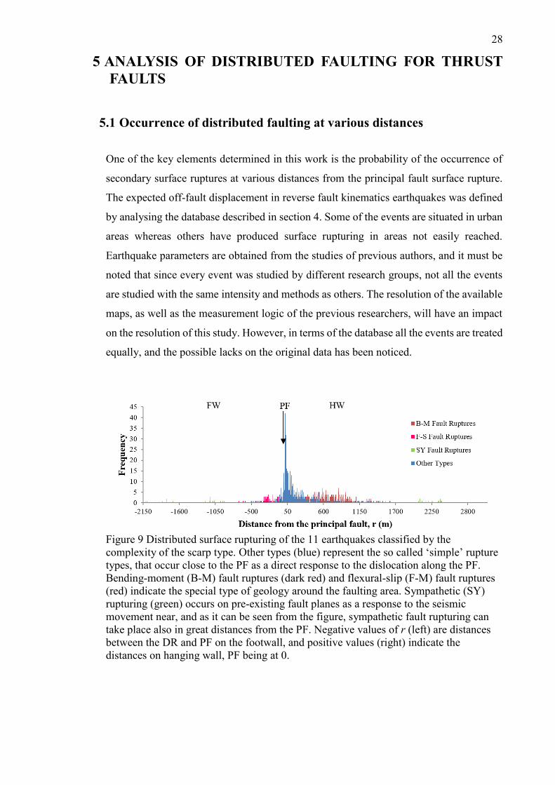
Figure 9 Distributed surface rupturing of the 11 earthquakes classified by the
complexity of the scarp type. Other types (blue) represent the so called ‘simple’ rupture
types, that occur close to the PF as a direct response to the dislocation along the PF.
Bending-moment (B-M) fault ruptures (dark red) and flexural-slip (F-M) fault ruptures
(red) indicate the special type of geology around the faulting area. Sympathetic (SY)
rupturing (green) occurs on pre-existing fault planes as a response to the seismic
movement near, and as it can be seen from the figure, sympathetic fault rupturing can
take place also in great distances from the PF. Negative values of r (left) are distances
between the DR and PF on the footwall, and positive values (right) indicate the
distances on hanging wall, PF being at 0.
29
Figure 9 represents the frequency of secondary surface fault rupturing of the 11 thrust
earthquakes as a function of distance from the main fault classified by the complexity of
the scarp. It can be noticed that these more complex types of secondary faults occur at
distances significantly greater than that of those ‘simple’ fault scarp types. When
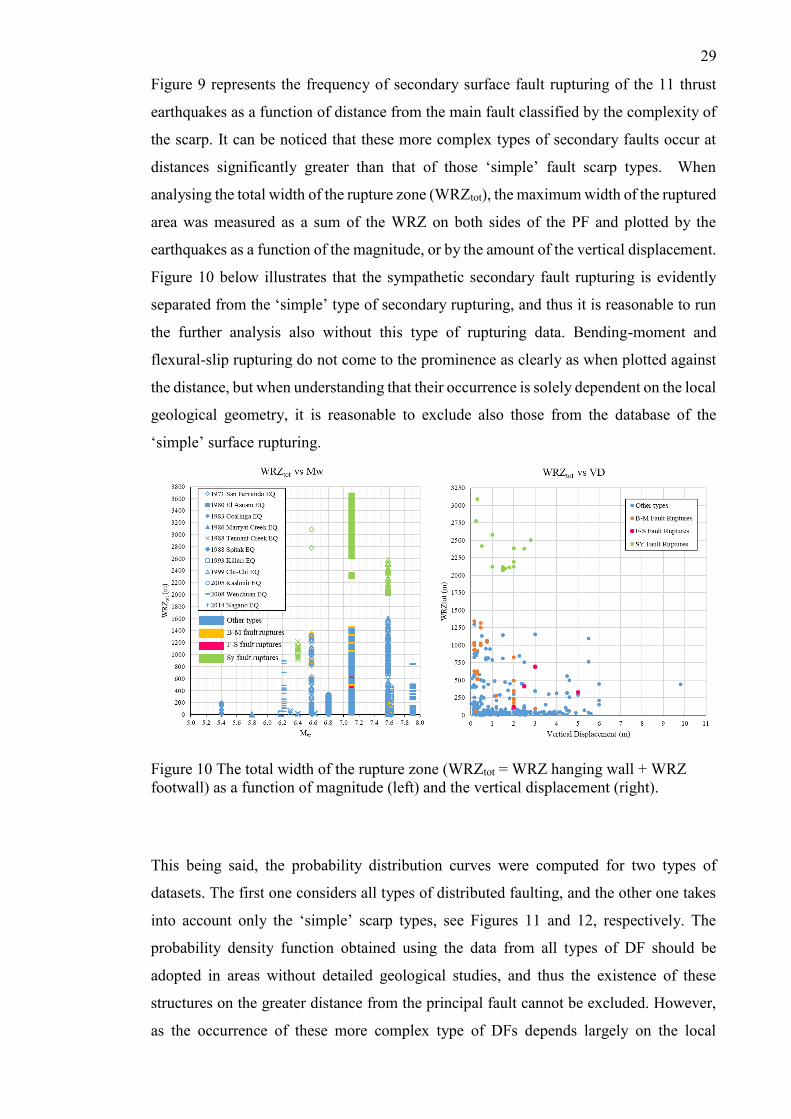
analysing the total width of the rupture zone (WRZtot), the maximum width of the ruptured
area was measured as a sum of the WRZ on both sides of the PF and plotted by the
earthquakes as a function of the magnitude, or by the amount of the vertical displacement.
Figure 10 below illustrates that the sympathetic secondary fault rupturing is evidently
separated from the ‘simple’ type of secondary rupturing, and thus it is reasonable to run
the further analysis also without this type of rupturing data. Bending-moment and
flexural-slip rupturing do not come to the prominence as clearly as when plotted against
the distance, but when understanding that their occurrence is solely dependent on the local
geological geometry, it is reasonable to exclude also those from the database of the
‘simple’ surface rupturing.
Figure 10 The total width of the rupture zone (WRZtot = WRZ hanging wall + WRZ
footwall) as a function of magnitude (left) and the vertical displacement (right).
This being said, the probability distribution curves were computed for two types of
datasets. The first one considers all types of distributed faulting, and the other one takes
into account only the ‘simple’ scarp types, see Figures 11 and 12, respectively. The
probability density function obtained using the data from all types of DF should be
adopted in areas without detailed geological studies, and thus the existence of these
structures on the greater distance from the principal fault cannot be excluded. However,
as the occurrence of these more complex type of DFs depends largely on the local
30
geological conditions, the probability of the existence of these DF on large distances
depend mainly on the presence of pre-existing fault structures (sympathetic faults), or
large-scale folding of hundreds of meters to kilometres in wavelength (bending-moment
or flexural slip fault structures). For the areas where the geological structure is well
studied, the expected seismic risk can be reduced taking into consideration only the DF
directly caused by the dislocation along the PF, calculating the distribution only for the
so called ‘simple’ secondary structures.
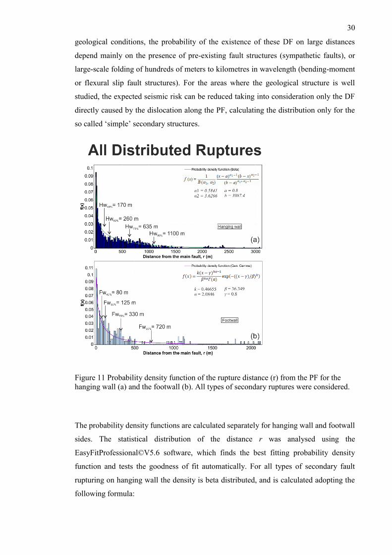
Figure 11 Probability density function of the rupture distance (r) from the PF for the
hanging wall (a) and the footwall (b). All types of secondary ruptures were considered.
The probability density functions are calculated separately for hanging wall and footwall
sides. The statistical distribution of the distance r was analysed using the
EasyFitProfessional©V5.6 software, which finds the best fitting probability density
function and tests the goodness of fit automatically. For all types of secondary fault
rupturing on hanging wall the density is beta distributed, and is calculated adopting the
following formula:
31
𝑓(𝑥) = 1
𝐵(𝛼1, 𝛼2)
(𝑥 − 𝑎)𝛼1−1(𝑏 − 𝑥)𝛼2−1
(𝑏 − 𝑎)𝛼1+𝛼2−1 , [5]
with the coefficients 1 = 0,5841, 2 = 3,6266, a = 0,8 and b = 3087,4. The probability of
distributed rupturing on the footwall on the other hand is gamma distributed:
𝑓(𝑥) =𝑘(𝑥 − 𝛾)𝑘𝛼−1
𝛽𝑘𝛼(𝑎)exp [− (
𝑥 − 𝛾𝛽⁄ )
𝑘
], [6]
where the coefficients are k = 0,46655, = 2,0846, = 36,349 and = 0,8.
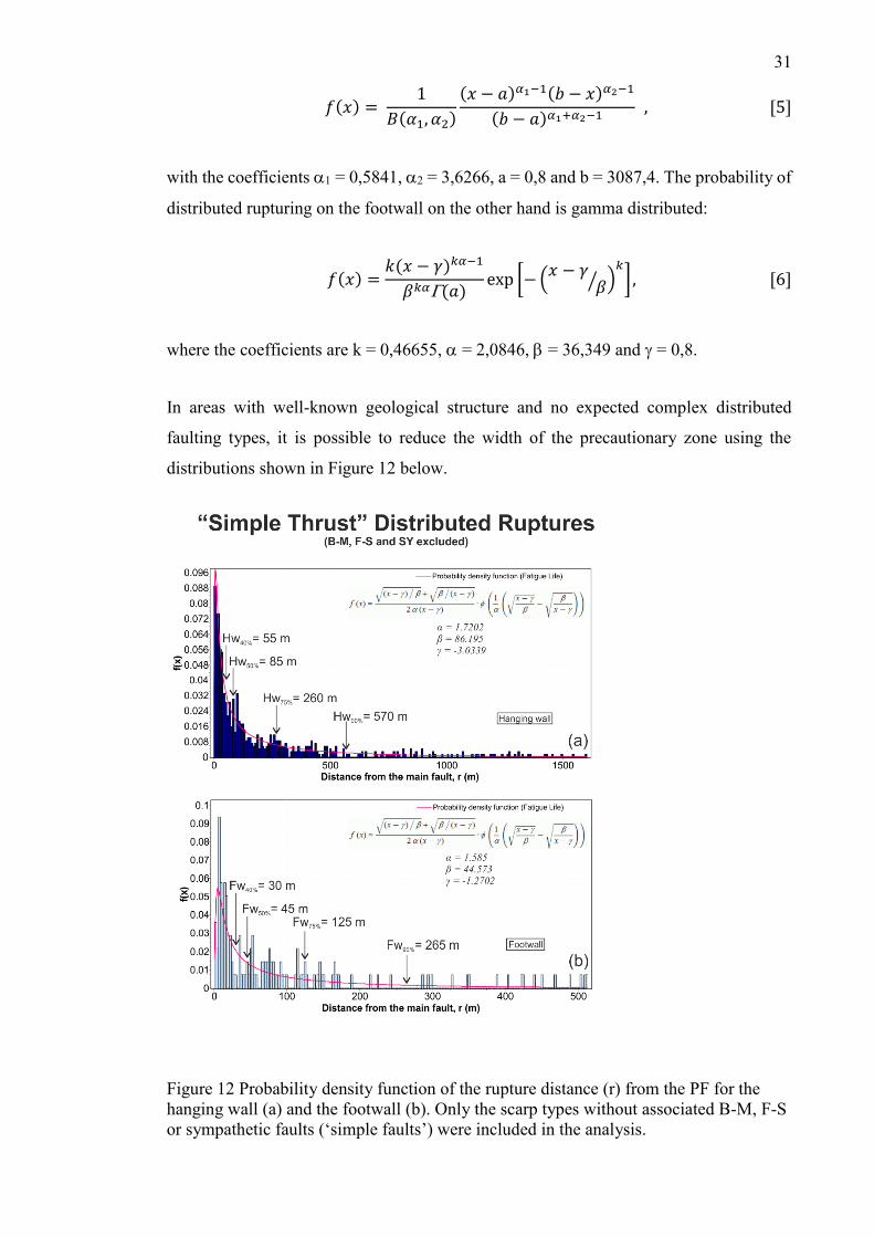
In areas with well-known geological structure and no expected complex distributed
faulting types, it is possible to reduce the width of the precautionary zone using the
distributions shown in Figure 12 below.
Figure 12 Probability density function of the rupture distance (r) from the PF for the
hanging wall (a) and the footwall (b). Only the scarp types without associated B-M, F-S
or sympathetic faults (‘simple faults’) were included in the analysis.
32
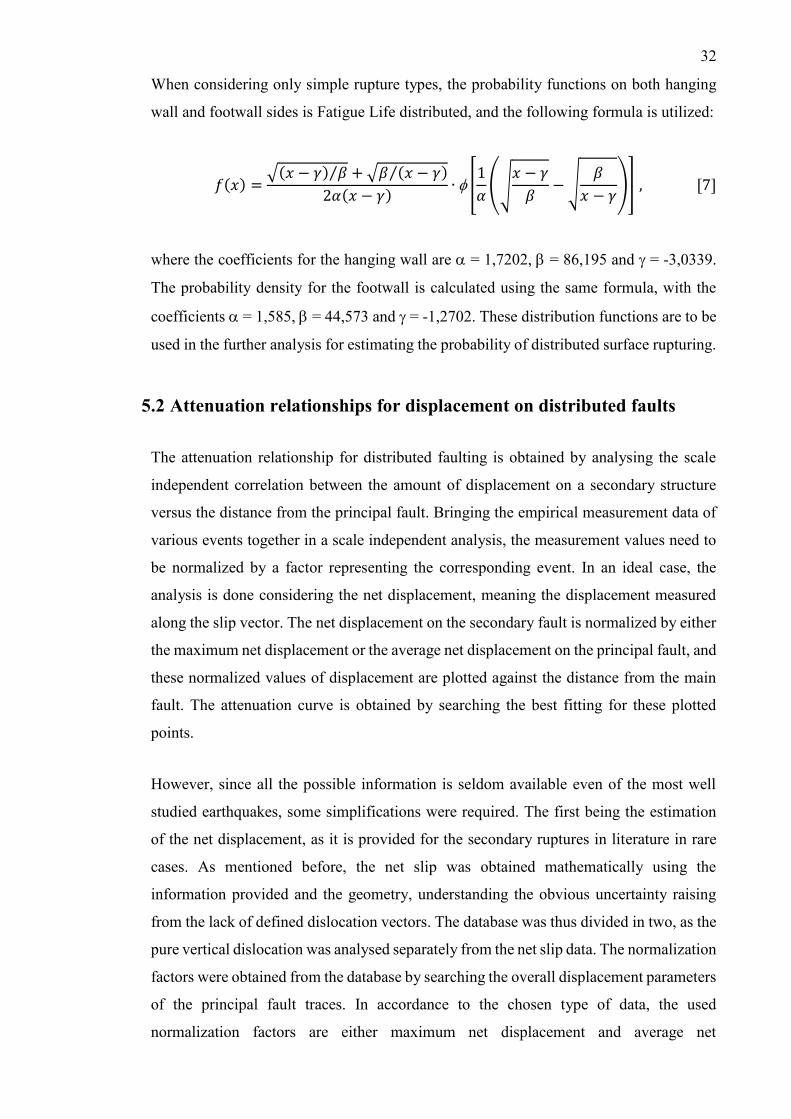
When considering only simple rupture types, the probability functions on both hanging
wall and footwall sides is Fatigue Life distributed, and the following formula is utilized:
𝑓(𝑥) =√(𝑥 − 𝛾) 𝛽⁄ + √𝛽 (𝑥 − 𝛾)⁄
2𝛼(𝑥 − 𝛾)∙ [
1
𝛼(√
𝑥 − 𝛾
𝛽− √
𝛽
𝑥 − 𝛾)] , [7]
where the coefficients for the hanging wall are = 1,7202, = 86,195 and = -3,0339.
The probability density for the footwall is calculated using the same formula, with the
coefficients = 1,585, = 44,573 and = -1,2702. These distribution functions are to be
used in the further analysis for estimating the probability of distributed surface rupturing.
5.2 Attenuation relationships for displacement on distributed faults
The attenuation relationship for distributed faulting is obtained by analysing the scale
independent correlation between the amount of displacement on a secondary structure
versus the distance from the principal fault. Bringing the empirical measurement data of
various events together in a scale independent analysis, the measurement values need to
be normalized by a factor representing the corresponding event. In an ideal case, the
analysis is done considering the net displacement, meaning the displacement measured
along the slip vector. The net displacement on the secondary fault is normalized by either
the maximum net displacement or the average net displacement on the principal fault, and
these normalized values of displacement are plotted against the distance from the main
fault. The attenuation curve is obtained by searching the best fitting for these plotted
points.
However, since all the possible information is seldom available even of the most well
studied earthquakes, some simplifications were required. The first being the estimation
of the net displacement, as it is provided for the secondary ruptures in literature in rare
cases. As mentioned before, the net slip was obtained mathematically using the
information provided and the geometry, understanding the obvious uncertainty raising
from the lack of defined dislocation vectors. The database was thus divided in two, as the
pure vertical dislocation was analysed separately from the net slip data. The normalization
factors were obtained from the database by searching the overall displacement parameters
of the principal fault traces. In accordance to the chosen type of data, the used
normalization factors are either maximum net displacement and average net

33
displacement, or maximum vertical displacement and average vertical displacement on
the principal fault. To provide further evidence of choosing the most adequate
normalization factor, the data of pure vertical dislocation was normalized also to
maximum net displacement, even if the data are not truly comparable.
At this point, it is important to emphasize that when creating the database, not all the
events were studied with the same accuracy on the principal surface rupture trace, due to
the reasons explained in the beginning of Chapter 4. In case of the events for which the
database was lacking the consistent data along the main fault, the values published in
previous literature of MD and AD were utilized. However, amongst all the articles read,
none of the authors defined explicitly which type of average was meant when reporting
an average displacement. This lead to the problem of the most accurate normalization
factor to be used, which will be viewed in following.
5.2.1 Obtaining the normalization factors
To be statistically analysable independent of the earthquake, the displacement data along
a secondary fault rupture must be normalized by some general parameter of the event, i.e.
by either maximum or average displacement along the principal fault rupture. Wells &
Coppersmith (1994) studied the dependence between magnitude and average or
maximum displacement, which both showed strong linear variation with magnitude in
normal and strike-slip movements, but reverse slip mechanism does not present as strong
dependence between these values. These equations for average and maximum
displacement of thrust earthquake fault slip were updated by their coefficients by Moss
and Ross (2011). They suggested the following formulas for calculating the average and
maximum displacement for the earthquake scenarios of defined magnitude:
log(𝐴𝐷) = 0.3244𝑀 − 2.2192 [8]
log(𝑀𝐷) = 0.5102𝑀 − 3.1971 [9]
As I had a database of empirical data in use, I chose to use it for determining the average
and maximum displacements for the events. Obtaining a maximum or average value of
any given group of numbers is a linear operation, but when talking about dislocation
parameters of an earthquake surface fault rupture, it is not as straight-forward calculation
in practice. Geological field work made by various study groups utilizing different
34
methods and measurement logics is not so easily confronted with these ‘simple’ factors,
as there is always some interpretation present – and some information is helplessly
lacking in almost every studied event. Most of the published materials regarding the older
seismic events contain only information of the vertical dislocation, and other dislocation
parameters have not been reported. Here, the calculations of net displacements are done
with the best information available, but when all the vectors are not defined, some
assumptions are unavoidably done for example considering the dip angle, if not provided.
Hypothetically speaking, the net slip provides more realistic information of the surface
rupturing, but the reliability of calculating these values using various assumptions when
a great deal of data is lacking diminishes significantly the trustworthiness of the net slip.
Maximum displacement
Previous authors have shown that using either AD or MD as a normalization factor are
both statistically valid approaches (see for example Moss & Ross, 2011). However, use
of either of these brings up different uncertainties that must be considered. The location
of the maximal surface slip along the principal fault rupture trace does not correlate with
the location of the epicentre in any systematic manner, and it has been observed from the
past earthquakes that the surface-slip distribution is better described by asymmetric rather
than symmetric curve forms (Wesnousky, 2008). Thus, MD is only a local value that
describes poorly the overall spatial distribution of the dislocation along the fault rupture.
Moreover, it is common that the different dislocation components, i.e. the maximum
vertical and the maximum horizontal component are measured in different locations along
the rupture (Wells & Coppersmith, 1994). However, MD is a value provided in similar
manner in every case: the highest value reported, even though various groups may have
different values of MD measured from the same event. Variability in the values of MD
does not necessarily mean that some authors had an error in their measurements, it might
also be that the working groups included different parts of the fault trace into their
investigation. Similarly, any given value of MD is only a maximum value among the
reported measurement points, as none of the fault scarps has been studied inch by inch.
Nevertheless, it is more than likely that the areas with the largest dislocation have been
of interest of the researchers, and scarps of the greatest displacement can be expected to
be measured, at least when interpreted to be caused by a co-seismic dislocation on the
principal fault plane and not by some another type of surface deformation.
35
Average displacement
Theoretically speaking, average displacement is a better representing value of the overall
fault displacement during an earthquake event, whereas the maximum displacement
represents the supreme dislocation and is often a single peak value largely influenced by
the local geology. Especially in cases of large earthquakes with long surface rupture, the
average value describes better the overall movement along the fault trace than the
maximum dislocation. However, it is not indifferent how the average is calculated. The
previous authors refer to the average displacement, but very few of them explain which
sort of average they mean. For example, in the model of Moss & Ross (2011), the
calculation of the displacement along the main fault is done based on the well estimated
average, but the authors do not specify which type of average they calculated. As the
authors demonstrated, it does not affect much on the result which value, AD or MD is
used in normalization of the dislocation on distributed faults, but it is important to
understand the problematics that relate to the estimation of these values in real life cases.
The most accurate method for defining the average displacement along the fault trace
would be dividing the integral along the fault by the length of the rupture. This requires
dislocation data from the measurement points with location defined in reasonable interval
along the whole length of the fault. However, in many historical earthquakes all this
information is not available, and it is not easily estimated from the published material.
Especially the events with the longest surface rupture traces and/or fault zones in distant
locations are not systematically measured along the whole extent of the fault which would
bring uncertainty to the integral. In addition, not all the principal fault surface ruptures
are exactly linear and continuous, and thus accurate estimation of the average
displacement would require also considering the faulting geometry. Understanding that
this would be theoretically the most correct approach, it must be ruled out due to lacks in
the availability of the information and the time need for estimating it from the insufficient
data existing. Wells & Coppersmith (1994) mention several graphical methods for
determining the average dislocation, but the problem in use of any of those is often lack
of precise, point related data, or that using them would be extremely time consuming.
Nevertheless, this should be kept in mind when taking the measures of the future
earthquake fault ruptures. In the following I represent three more simple types of averages
that were used in this work.
36
Arithmetic average, ADa
Arithmetic mean, the classical type of average value, is calculated by dividing the sum of
all displacement values reported by the total number of measurement points associated
with the displacement information. This is the mean value of the local displacement
values and does not consider the geometry or the location along the principal fault, or the
possible gaps of measurements along the fault with no displacement data. It was pointed
out already by Well & Coppersmith (1994) that taking a simple average of displacement
measurement values does not represent the true average surface displacement along the
fault very well. The problem is often that there is no data from regular interval along all
the length of the fault, and there may be unreachable areas with no displacement data
along the fault trace. This should be compensated by using some other way of determining
the average.
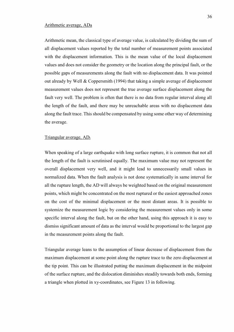
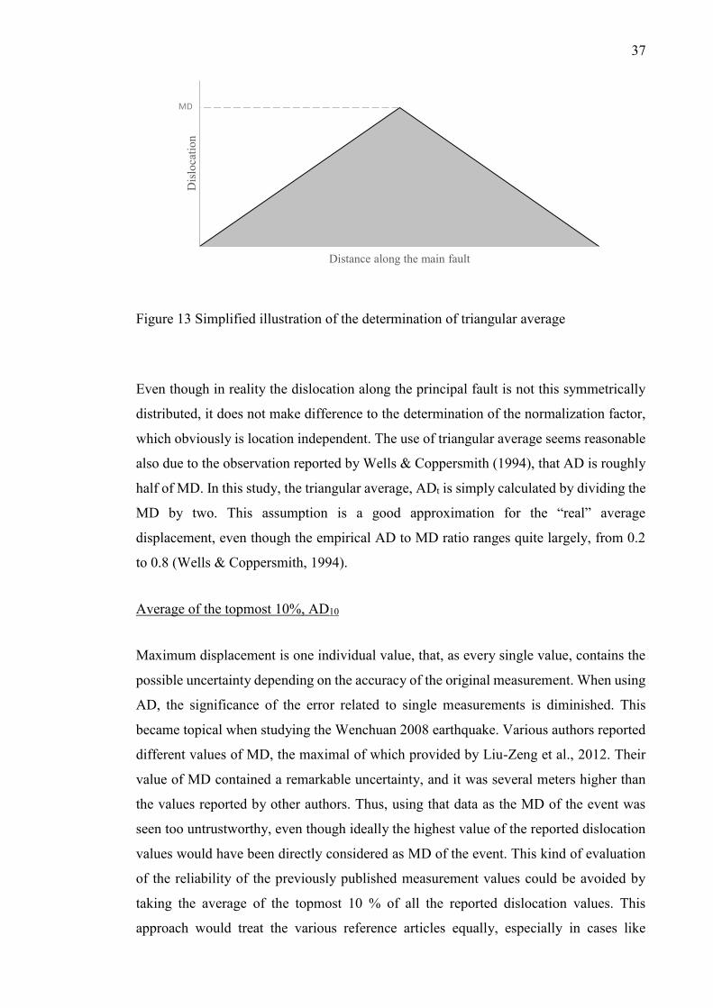
Triangular average, ADt
When speaking of a large earthquake with long surface rupture, it is common that not all
the length of the fault is scrutinised equally. The maximum value may not represent the
overall displacement very well, and it might lead to unnecessarily small values in
normalized data. When the fault analysis is not done systematically in same interval for
all the rupture length, the AD will always be weighted based on the original measurement
points, which might be concentrated on the most ruptured or the easiest approached zones
on the cost of the minimal displacement or the most distant areas. It is possible to
systemize the measurement logic by considering the measurement values only in some
specific interval along the fault, but on the other hand, using this approach it is easy to
dismiss significant amount of data as the interval would be proportional to the largest gap
in the measurement points along the fault.
Triangular average leans to the assumption of linear decrease of displacement from the
maximum displacement at some point along the rupture trace to the zero displacement at
the tip point. This can be illustrated putting the maximum displacement in the midpoint
of the surface rupture, and the dislocation diminishes steadily towards both ends, forming
a triangle when plotted in xy-coordinates, see Figure 13 in following.
37
Figure 13 Simplified illustration of the determination of triangular average
Even though in reality the dislocation along the principal fault is not this symmetrically
distributed, it does not make difference to the determination of the normalization factor,
which obviously is location independent. The use of triangular average seems reasonable
also due to the observation reported by Wells & Coppersmith (1994), that AD is roughly
half of MD. In this study, the triangular average, ADt is simply calculated by dividing the
MD by two. This assumption is a good approximation for the “real” average
displacement, even though the empirical AD to MD ratio ranges quite largely, from 0.2
to 0.8 (Wells & Coppersmith, 1994).
Average of the topmost 10%, AD10
Maximum displacement is one individual value, that, as every single value, contains the
possible uncertainty depending on the accuracy of the original measurement. When using
AD, the significance of the error related to single measurements is diminished. This
became topical when studying the Wenchuan 2008 earthquake. Various authors reported
different values of MD, the maximal of which provided by Liu-Zeng et al., 2012. Their
value of MD contained a remarkable uncertainty, and it was several meters higher than
the values reported by other authors. Thus, using that data as the MD of the event was
seen too untrustworthy, even though ideally the highest value of the reported dislocation
values would have been directly considered as MD of the event. This kind of evaluation
of the reliability of the previously published measurement values could be avoided by
taking the average of the topmost 10 % of all the reported dislocation values. This
approach would treat the various reference articles equally, especially in cases like
Dis
loca
tio
n
Distance along the main fault
MD
38
Wenchuan where the different research groups were clearly measuring in different
locations.
But why 10 %, why not 5 or 20 %? The events chosen in this database are various in size:
the total rupture length along the PF varies between 3.3 to 240 kilometres, thus also the
amount of measurement points vary quite remarkably from an event to another. The
approach suggested here in cases of small events is closer to the approach of normalizing
with the pure MD, as topmost 10% means in practise only a couple of values, but this
approach was invented to eliminate the possibly high uncertainty of a single value
especially in large events perhaps studied by various research groups – and none of them
from the entire length of the rupture. In some smaller cases, the top most 10 % would in
practice mean only the one highest value, but these faults can be assumed well studied
along the whole extent of the rupture trace and no big uncertainties between the sources
of data should remain anyway. In practice the topmost 10 % average was calculated by
taking the arithmetic average of the highest 10% of the dislocation values reported along
the PF. This method was invented during the work and its suitability has not been tested
previously. It was decided to be kept along in the further analysis since there was no
explicitly good option for the normalization in use, and the comparison between the
different normalization factors was about to be done anyway.
Summary of calculated normalization parameters
The events and the corresponding normalization factors from the dislocation along the
principal faults are listed in Table 3. The values are either obtained from the database
compiled during this work, or taken directly from literature, especially in cases where the
database was not comprehensible all the way along the principal fault rupture. These cases
were explained more in detail in Chapter 4. At this point it is reasonable to point out that
amount of dislocation for distributed surface fault rupturing has not been reported for all
the 11 earthquakes included in the complete database and thus these events were naturally
cancelled out from the analysis of the attenuation relationships of the amount of
dislocation. The events with no measured dislocation along the DF were 1986 Marryat
Creek and 1988 Spitak earthquakes. Consequently, there was no need for the
normalization factors for these events.

39
Table 3 List of the earthquakes and the dislocation parameters along the principal fault
rupture
MDv is the maximum value of vertical dislocation along all the main fault, which might
have been measured also in a point with no directly associated distributed faulting. Thus,
the maximum value might also be found in a point not considered in the previously
published database (see Boncio et al., 2018 Table S1), especially in cases which were
studied concentrating only on the distributed faulting. The following three columns
represent the calculated values of different types of average displacement along the main
fault, ADa, ADt and AD10, calculated from the vertical dislocation. The last four columns
on the right-hand side of the table contain the similar normalization factors for the net
dislocation along the principal fault.
5.2.2 Obtaining the dislocation distribution
The earthquake catalogues provide mainly information of the vertical displacement, but
especially in cases of very low angle thrusts, vertical dislocation does not represent the
amount of the total movement of the main fault very well. For the principal fault
displacement, net displacement listed in the table above was calculated as a vector sum
of the reported dislocation parameters or using the basic geometry and the dip angle when
not all the parameters were clearly defined. For the systematic analysis of the events, only
the equal type of data could be confronted, meaning that the normalization factor should
be of the similar sense of movement as the displacement that is normalized. The
estimation of the net slip along the secondary structures is more complex as their
orientation and dip angles may vary significantly from the ones of the main fault.
Considering that the specific data of the slip vectors is rarely provided, the geometry-
based method was not used for estimating the net slip on distributed faulting. For DF, the
Earthquake Date
Mw
MD
v
AD
a v
AD
t, v
AD
10 v
MD
n
AD
a n
AD
t n
AD
10 n
San Fernando, CA, USA 1971/02/09 6.6 0.76 0.31 0.38 0.75 2.27 0.94 1.13 2.03
El Asnam, Algeria 1980/10/10 7.1 5.00 1.95 2.5 5.00 6.5 1.2 3.25 10
Coalinga (Nuñez), CA, USA 1983/06/11 5.4 0.50 0.17 0.25 0.44 1.0 0.34 0.50 0.91
Tennant Creek, Australia 1988/01/22
(3 events)
6.3
6.4
6.6
1.20
1.10
1.77
0.75
1.10
1.47
0.60
0.55
0.88
1.20
1.10
1.70
2.84
2.60
2.50
1.79
1.66
2.29
1.42
1.30
1.25
2.84
2.60
2.50
Killari, India 1993/09/29 6.2 0.60 0.53 0.30 0.60 1.20 1.05 0.60 1.20
Chi Chi, Taiwan 1999/09/20 7.6 12.7 2.49 4.90 5.18 16.4 4.67 6.0 9.20
Kashmir, Pakistan 2005/10/08 7.6 3.40 1.82 1.70 3.40 7.05 3.80 3.4 6.8
Wenchuan, China 2008/05/12 7.9 6.90 1.85 3.45 4.71 13.0 3.49 6.5 8.94
Nagano, Japan 2014/11/22 6.2 0.80 0.43 0.40 0.80 1.60 0.65 0.80 1.60
40
net slip was assumed to be a simple vector sum of the dislocation parameters given at the
same location reported by the previous authors. In practise this mean that when some
dislocation component was not reported, that was assumed to zero.
The attenuation curves were obtained by analysing the database values using Matlab, all
the sub-databases separately. The selected data was plotted against the distance from the
PF, and the attenuation relationships were found from fitting that would represent the
attenuation of the surface dislocation distribution. Various approaches for obtaining the
attenuation curves for secondary surface rupturing were tested during this work. Creating
a model based on empirical data is not a straightforward operation, but the working
methods and especially the delimitations regarding the data used could only be done as
the work proceeded.
The hypothesis before beginning the work was that when plotting the dislocation on
secondary rupturing as a function of the distance from the principal fault, the peak of the
density is found relatively close, but not exactly right next to the main fault. A plausible
explanation is that the principal fault surface rupturing is a local energy release maximum,
and it is unlikely to have secondary rupturing right next to it, but after a kind of a “shadow
zone”. Thus, the expectation was to obtain a fitting curve with a peak in some distance
from the PF, after which it decreases somewhat exponentially along the distance
approaching zero in distance depending from the chosen database. The form of the curve
is expected to be more or less similar on both sides of the fault, but the distribution on the
footwall is narrower in distance, and smaller in amplitude. Youngs et al. (2003, fig. 11)
reported the upper bound curves of the maximum displacement distribution curves, which
was the base of the hypothesis also in this work. However, their analysis wan lengthened
up till 20 kilometres distance on both hanging wall and footwall, so the database used was
clearly established by different criterion than in this work.
All the previously mentioned normalization factors were tested to choose the one that
gives the best response on curve fitting. The data grouped to vertical and net slip sub-
databases were normalized by corresponding maximum and three average values. All the
data points were fitted by using two-term exponential fit [10] and gaussian fit [11]:
𝑓(𝑥) = 𝑎 𝑒𝑏𝑥 + 𝑐 𝑒𝑑𝑥 [10]
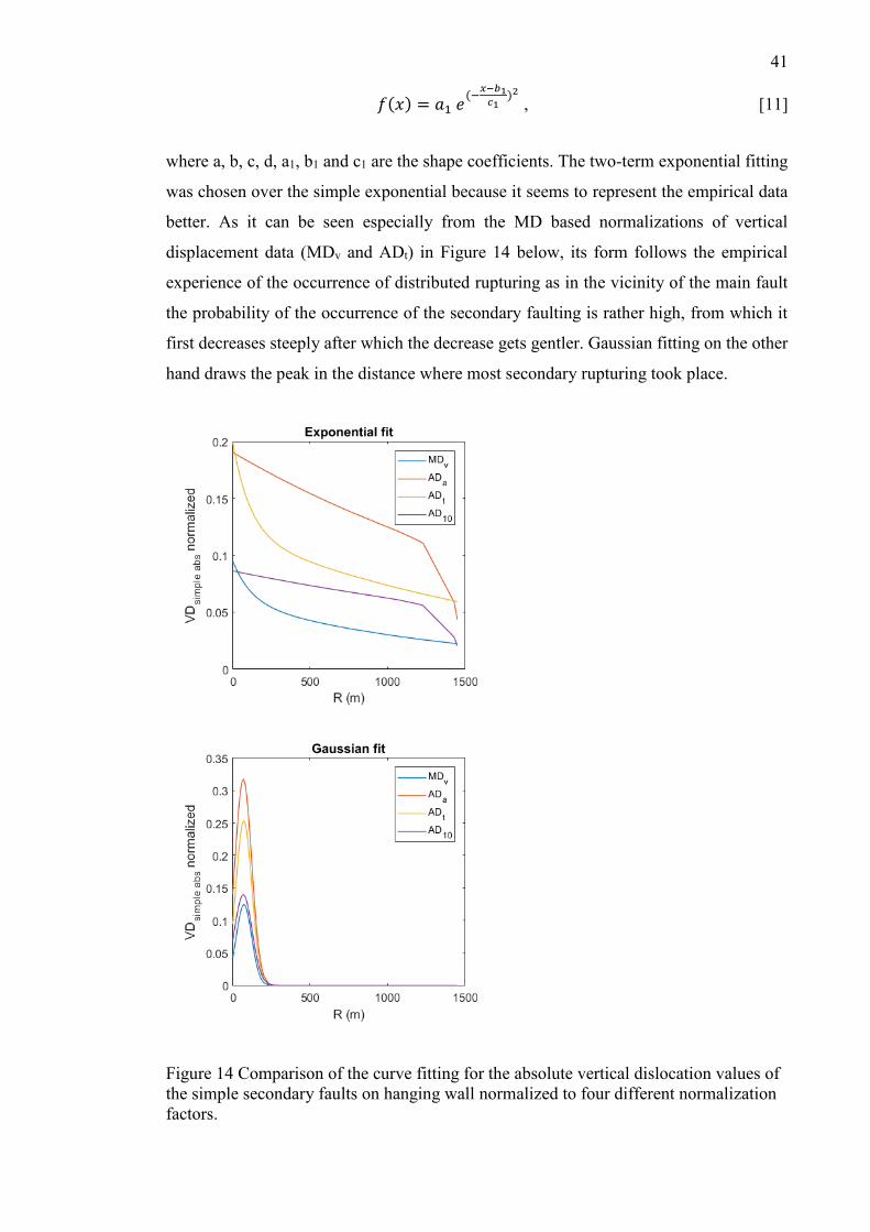
41
𝑓(𝑥) = 𝑎1 𝑒(−
𝑥−𝑏1𝑐1
)2
, [11]
where a, b, c, d, a1, b1 and c1 are the shape coefficients. The two-term exponential fitting
was chosen over the simple exponential because it seems to represent the empirical data
better. As it can be seen especially from the MD based normalizations of vertical
displacement data (MDv and ADt) in Figure 14 below, its form follows the empirical
experience of the occurrence of distributed rupturing as in the vicinity of the main fault
the probability of the occurrence of the secondary faulting is rather high, from which it
first decreases steeply after which the decrease gets gentler. Gaussian fitting on the other
hand draws the peak in the distance where most secondary rupturing took place.
Figure 14 Comparison of the curve fitting for the absolute vertical dislocation values of
the simple secondary faults on hanging wall normalized to four different normalization
factors.
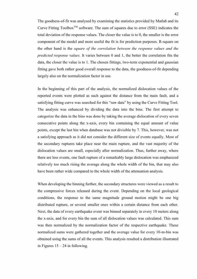
42
The goodness-of-fit was analysed by examining the statistics provided by Matlab and its
Curve Fitting ToolboxTM software. The sum of squares due to error (SSE) indicates the
total deviation of the response values. The closer the value is to 0, the smaller is the error
component of the model and more useful the fit is for prediction purposes. R-square on
the other hand is the square of the correlation between the response values and the
predicted response values. It varies between 0 and 1, the better the correlation fits the
data, the closer the value is to 1. The chosen fittings, two-term exponential and gaussian
fitting gave both rather good overall response to the data, the goodness-of-fit depending
largely also on the normalization factor in use.
In the beginning of this part of the analysis, the normalized dislocation values of the
reported events were plotted as such against the distance from the main fault, and a
satisfying fitting curve was searched for this “raw data” by using the Curve Fitting Tool.
The analysis was enhanced by dividing the data into the bins. The first attempt to
categorize the data in the bins was done by taking the average dislocation of every seven
consecutive points along the x-axis, every bin containing the equal amount of value
points, except the last bin when database was not divisible by 7. This, however, was not
a satisfying approach as it did not consider the different size of events equally. Most of
the secondary ruptures take place near the main rupture, and the vast majority of the
dislocation values are small, especially after normalization. Thus, further away, where
there are less events, one fault rupture of a remarkably large dislocation was emphasized
relatively too much rising the average along the whole width of the bin, that may also
have been rather wide compared to the whole width of the attenuation analysis.
When developing the binning further, the secondary structures were viewed as a result to
the compressive forces released during the event. Depending on the local geological
conditions, the response to the same magnitude ground motion might be one big
distributed rupture, or several smaller ones within a certain distance from each other.
Next, the data of every earthquake event was binned separately in every 10 meters along
the x-axis, and for every bin the sum of all dislocation values was calculated. This sum
was then normalized by the normalization factor of the respective earthquake. These
normalized sums were gathered together and the average value for every 10-m-bin was
obtained using the sums of all the events. This analysis resulted a distribution illustrated
in Figures 15 – 24 in following.
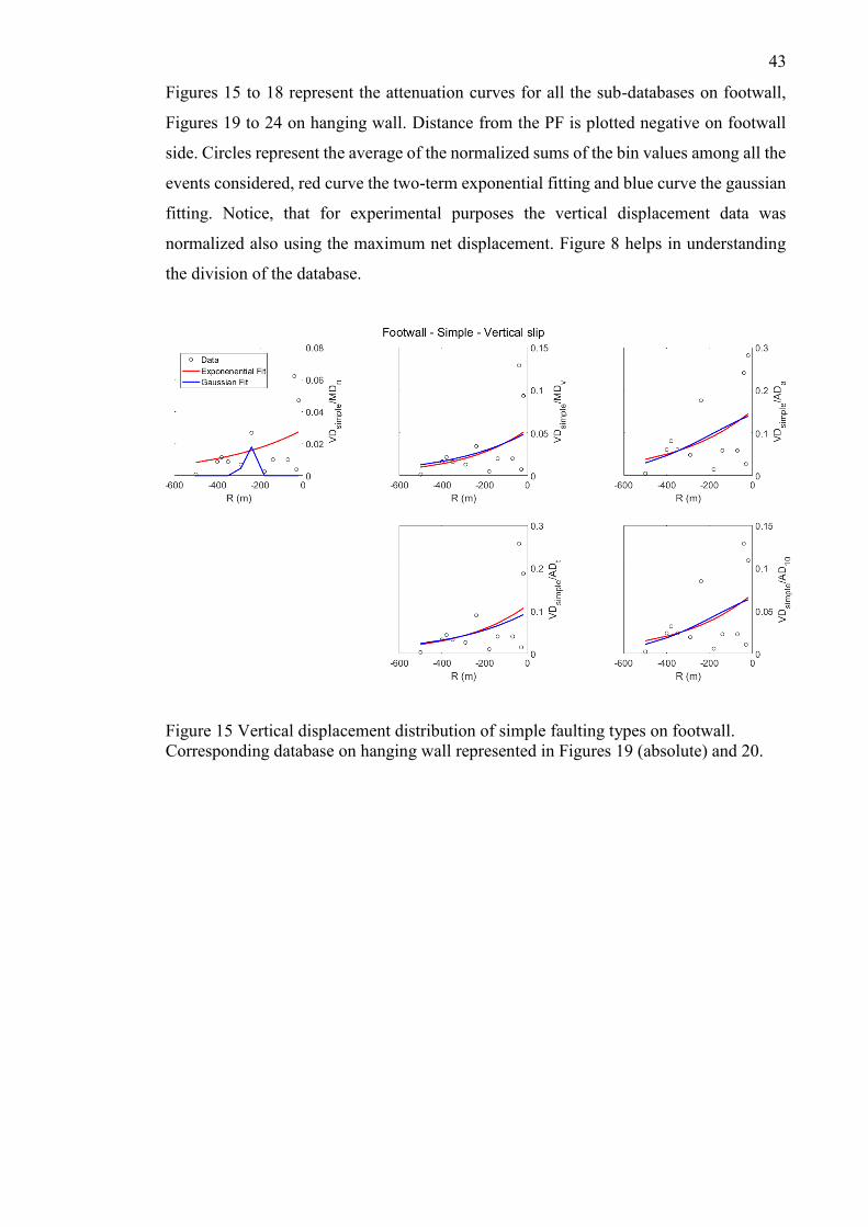
43
Figures 15 to 18 represent the attenuation curves for all the sub-databases on footwall,
Figures 19 to 24 on hanging wall. Distance from the PF is plotted negative on footwall
side. Circles represent the average of the normalized sums of the bin values among all the
events considered, red curve the two-term exponential fitting and blue curve the gaussian
fitting. Notice, that for experimental purposes the vertical displacement data was
normalized also using the maximum net displacement. Figure 8 helps in understanding
the division of the database.
Figure 15 Vertical displacement distribution of simple faulting types on footwall.
Corresponding database on hanging wall represented in Figures 19 (absolute) and 20.

44
Figure 16 Net displacement distribution of simple faulting types on footwall.
Corresponding database on hanging wall represented in Figure 21.
Figure 17 Vertical displacement distribution of all faulting types on footwall.
Corresponding database on hanging wall represented in Figures 22 (absolute) and 23.
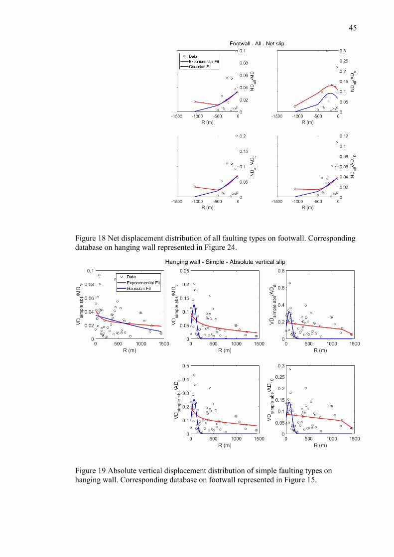
45
Figure 18 Net displacement distribution of all faulting types on footwall. Corresponding
database on hanging wall represented in Figure 24.
Figure 19 Absolute vertical displacement distribution of simple faulting types on
hanging wall. Corresponding database on footwall represented in Figure 15.
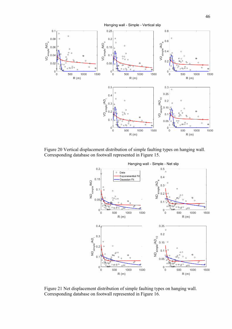
46
Figure 20 Vertical displacement distribution of simple faulting types on hanging wall.
Corresponding database on footwall represented in Figure 15.
Figure 21 Net displacement distribution of simple faulting types on hanging wall.
Corresponding database on footwall represented in Figure 16.

47
Figure 22 Absolute vertical displacement distribution of all faulting types on hanging
wall. Corresponding database on footwall represented in Figure 17.
Figure 23 Vertical displacement distribution of all faulting types on hanging wall.
Corresponding database on footwall represented in Figure 17.
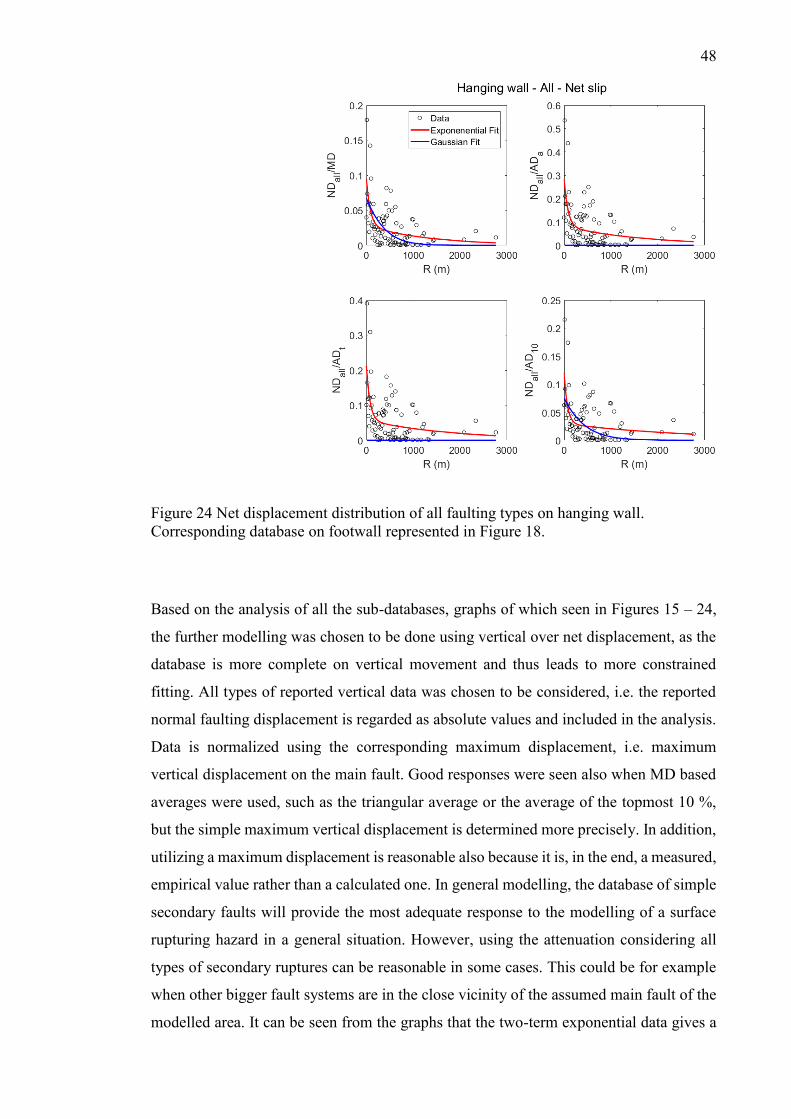
48
Figure 24 Net displacement distribution of all faulting types on hanging wall.
Corresponding database on footwall represented in Figure 18.
Based on the analysis of all the sub-databases, graphs of which seen in Figures 15 – 24,
the further modelling was chosen to be done using vertical over net displacement, as the
database is more complete on vertical movement and thus leads to more constrained
fitting. All types of reported vertical data was chosen to be considered, i.e. the reported
normal faulting displacement is regarded as absolute values and included in the analysis.
Data is normalized using the corresponding maximum displacement, i.e. maximum
vertical displacement on the main fault. Good responses were seen also when MD based
averages were used, such as the triangular average or the average of the topmost 10 %,
but the simple maximum vertical displacement is determined more precisely. In addition,
utilizing a maximum displacement is reasonable also because it is, in the end, a measured,
empirical value rather than a calculated one. In general modelling, the database of simple
secondary faults will provide the most adequate response to the modelling of a surface
rupturing hazard in a general situation. However, using the attenuation considering all
types of secondary ruptures can be reasonable in some cases. This could be for example
when other bigger fault systems are in the close vicinity of the assumed main fault of the
modelled area. It can be seen from the graphs that the two-term exponential data gives a
49
more realistic overall response to the data than the gaussian one. The probability of the
secondary rupturing is the highest close to the main fault, after which it first decreases
rapidly before stabilizing. The graphs showing the displacement distribution on footwall
are highly impacted by the fact that the sub-databases in some selections were very small.
For this reason, the fitting curves on footwall are not as smooth as on the hanging wall in
general. This could be enhanced by adding data of other earthquake events to the
database.
5.2.3 Obtaining the probability distribution
The probability distribution of secondary rupturing is obtained analysing the spatial
variability of the occurrence of the surface deformation. The analysis is done on top of a
shapefile of the mapped trace of the chosen principal fault, utilizing a grid of 10 x 10 m,
the reach depending on the chosen setting (‘simple’ or ‘all’). For each grid point is defined
the distance r to the main fault, and positioning either on hanging wall or footwall
according to the azimuth angle respect to the average direction of the principal fault. This
probability analysis is limited on distributed faulting only, thus the zone that can be
considered as principal fault surface rupture trace is excluded. In practice, the points with
a distance less or equal to 5 m from the principal fault rupture trace are cut out from the
grid, resulting the main fault zone of 10 m in total. The grid considers the fault trace
geometry better than dividing the fault surroundings into simple “slices” according to the
distance from the main fault, as the fault lines in nature cannot be treated as perfectly
straight lines in a detailed analysis. The grid is used in the following computation for
counting the seismic hazard parameters for each grid point independently.
The probability for surface rupturing is calculated utilizing a survival function (also
known as reliability, or complementary cumulative distribution function) for hanging
wall and footwall separately. At this point the reach is defined for both wall sides
separately, in ‘simple’ scenario distances being 1600 m for hanging wall and 500 m for
footwall. These distances are chosen from the empirical data of the events studied
previously in this work, so that all the reported secondary faulting is included in these
distances. The probability of surface faulting is computed utilizing the probability density
functions for surface rupturing, these obtained for the empirical database are shown in
Figures 11 and 12. Probability density function of simple types of secondary faulting was
fitted using Fatigue Life function for both footwall and hanging wall. The functions used
when also all the complex rupture types considered were beta distribution for the hanging

50
wall and generalized gamma distribution for the footwall. Survival function is the
cumulative sum function of the respective probability density function. As the vertical
displacement data was seen statistically more robust, the further modelling was done by
using the (absolute) vertical displacement data. In case of reliable net displacement data,
the following computations can be done equally utilizing the coefficients derived from
the net displacement data.
The probability is assessed for a certain scenario event, so at this point the good
knowledge of the fault system and the expected seismicity on the fault leads to more
realistic boundary conditions and thus to a better estimation of the future hazard. From
the well estimated SRL of a mapped fault we can obtain the expected magnitude and the
maximum dislocation for the event when the fault ruptures from its entire length. For
calculating the probability of exceedance (POE) of the given normalized vertical
displacement levels (VDL) for a point at a distance r from the PF, the maximum vertical
displacement, the VDLs and the number of sigma for the probability of vertical
displacement must be defined. VDLs used in PFDHA are equivalent of the intensity
measure level in PSHA modelling. The VDL values used here were from 1 cm to 50 cm
in 1 cm interval. The probability of the normalized vertical displacement at a distance r
from the principal fault is done utilizing the coefficients of the two-term exponential
fitting of the displacement data for simple absolute vertical displacement, illustrated in
Figures 15 and 19. For an event with a MD on the principal fault, the probability of
exceedance of a vertical measure for a site at a distance r is computed from the mean
vertical displacement value expected, and the uncertainty related to the measure.
Furthermore, the conditional probability of exceedance is computed by multiplying the
probability of faulting by the probability of exceedance.
The likelihood of the occurrence of distributed faulting can be plotted as a function of
distance from the PF as a percental probability. The probability of exceedance of given
displacement levels are plotted against the (vertical or net) displacement as such and using
the condition number for the given probability of the displacement at a defined distance.
In the model, the absolute and conditional probabilities of exceedance of VDL are plotted
in distances of 6, 10, 100 and 500 m from the main fault. At the 6 m distance are the first
grid points the model considers belonging to distributed faulting, as it was previously
decided that the principal fault zone equals 10 m wide zone, 5 m to both sides of the
rupture. The other distances are chosen arbitrarily.
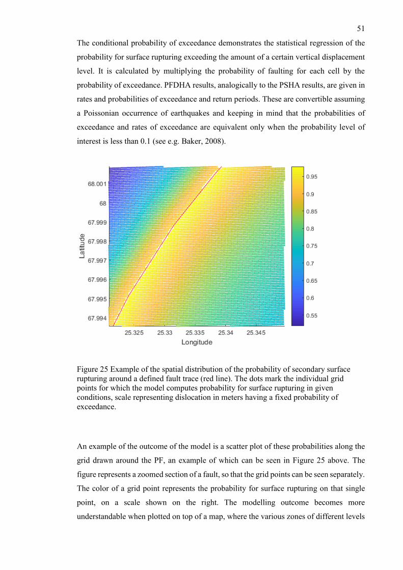
51
The conditional probability of exceedance demonstrates the statistical regression of the
probability for surface rupturing exceeding the amount of a certain vertical displacement
level. It is calculated by multiplying the probability of faulting for each cell by the
probability of exceedance. PFDHA results, analogically to the PSHA results, are given in
rates and probabilities of exceedance and return periods. These are convertible assuming
a Poissonian occurrence of earthquakes and keeping in mind that the probabilities of
exceedance and rates of exceedance are equivalent only when the probability level of
interest is less than 0.1 (see e.g. Baker, 2008).
Figure 25 Example of the spatial distribution of the probability of secondary surface
rupturing around a defined fault trace (red line). The dots mark the individual grid
points for which the model computes probability for surface rupturing in given
conditions, scale representing dislocation in meters having a fixed probability of
exceedance.
An example of the outcome of the model is a scatter plot of these probabilities along the
grid drawn around the PF, an example of which can be seen in Figure 25 above. The
figure represents a zoomed section of a fault, so that the grid points can be seen separately.
The color of a grid point represents the probability for surface rupturing on that single
point, on a scale shown on the right. The modelling outcome becomes more
understandable when plotted on top of a map, where the various zones of different levels

52
of hazard can be seen in the natural environment. The final modelling is done for the
amount of vertical displacement having the probability of 1% and 2% to be exceeded.
This is done in practice by re-sampling the curve for finding the closest VDL to the
desired probability of exceedance. The functioning of the model created here is
demonstrated in the following chapter where it is applicated to Suasselkä post-glacial
fault located in Northern Finland.
53
6 APPLICATION OF THE MODEL
The model is meant to be implemented on a mapped fault trace of an active tectonic fault
of reverse kinematics. In general, the accuracy of a fault location depends on the geologic
and geomorphic conditions and thus the ability of the geologists to recognize and interpret
the fault, but also the accuracy of transferring the information onto the base maps. The
implementation of the model requires either the knowledge of the seismic properties of
the considered fault (slip rate and expected magnitude), but when historical data not
available, those can also be estimated from the observed surface rupture trace. The
estimation should be done considering the uncertainties in size, specific location and types
of surface deformation. Thus, the implementation of the model can be done using the
scenario approach, where the magnitude of the event is the largest imagined, that is the
magnitude calculated from the total length of the fault assuming that surface rupturing
occurs: P(slip|m) = 1 (no blind faulting considered as an option), and that the fault
ruptures its total length (i.e. the surface rupture length, SRL; Wells & Coppersmith,
1994). Empirical observations of historical earthquakes have shown that not always the
faults rupture the entire length of the mapped fault but considering the total SRL is
reasonable in hazard analysis purposes. The chosen magnitude should be seen as a
“reasonably large” event, rather than “maximum credible earthquake”, MCE (also
“maximum considered earthquake”), as also bigger event on the fault is credible, yet less
probable (Baker, 2008). From the magnitude or from the expected SRL it is possible to
calculate the corresponding maximum displacement along the principal fault, which is a
key parameter to the further analysis of distributed fault hazard. It must be noted, though,
that for overall seismic hazard analysis including also the hazard along the principal fault,
MD may be used rather as an upper bound as its exact location is hard to predict (Wells
& Coppersmith, 1994). In this work the model is applied in Suasselkä post-glacial fault
in northern Fennoscandia.
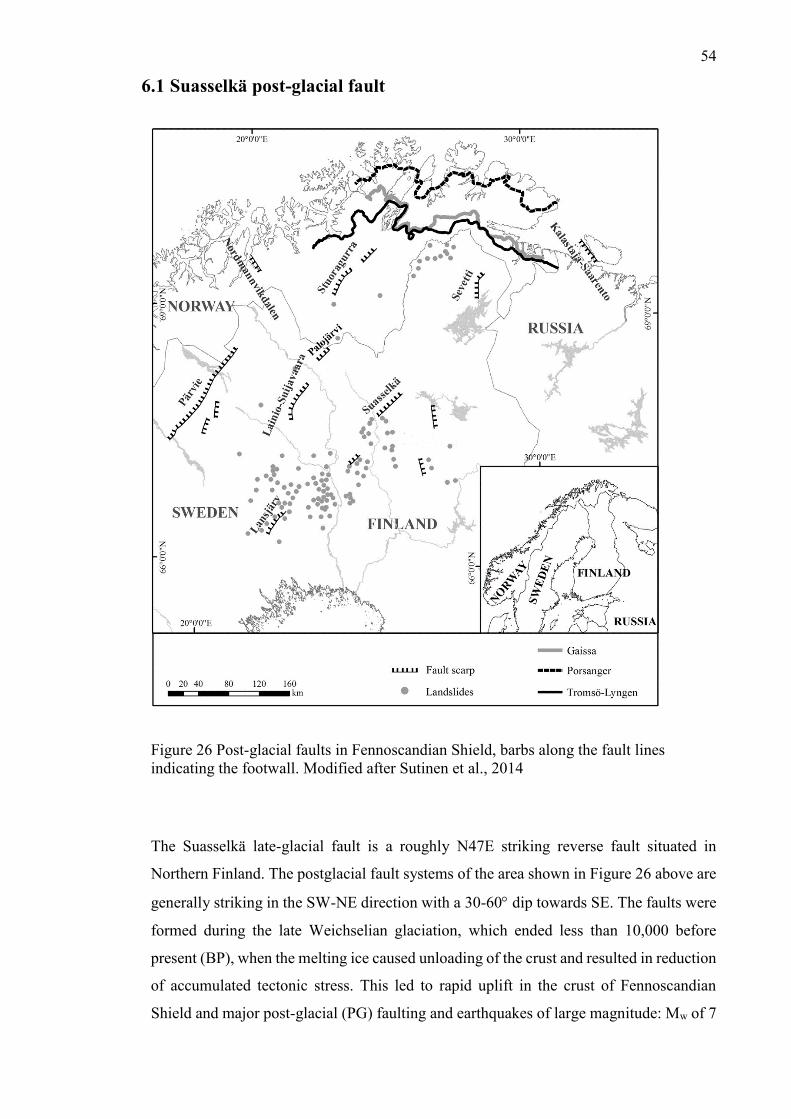
54
6.1 Suasselkä post-glacial fault
Figure 26 Post-glacial faults in Fennoscandian Shield, barbs along the fault lines
indicating the footwall. Modified after Sutinen et al., 2014
The Suasselkä late-glacial fault is a roughly N47E striking reverse fault situated in
Northern Finland. The postglacial fault systems of the area shown in Figure 26 above are
generally striking in the SW-NE direction with a 30-60 dip towards SE. The faults were
formed during the late Weichselian glaciation, which ended less than 10,000 before
present (BP), when the melting ice caused unloading of the crust and resulted in reduction
of accumulated tectonic stress. This led to rapid uplift in the crust of Fennoscandian
Shield and major post-glacial (PG) faulting and earthquakes of large magnitude: Mw of 7

55
– 8.2 (Afonin et al., 2017 referring to Wu et al., 1999, Olesen et al., 2004 and Kukkonen
et al., 2010). The faults of the system are from 2 up to 150 km-long, and the scarp height
varies from 1 up to 12 meters, the highest scarp reported being 30 meters (Sutinen et al.,
2014). Wu et al. (1999) suggested that the fault activity of the area begun 15,000 yrs BP,
the peak in seismic activity being between 13,000 – 10,000 yrs BP. Post-glacial faulting
occurred most likely between 10,500 – 10,000 yrs BP. LiDar (Light Detection and
Ranging) scanning and radiocarbon dating have been done on the area for mapping and
dating the fault activity, but the interpretations of the continuation of the seismicity after
the deglaciation vary significantly: from 2,000 up to 5,000 years after deglaciation (see
e.g. Paananen, 1987, Sutinen et al., 2014, Abdi et al., 2015) During the seismically active
period, the water in the fault planes has played a remarkable role in seismicity right after
the deglaciation, as the low friction allows slipping of the fault even if in conditions where
the crustal stress field is still insufficient for producing an earthquake by itself. (Abdi et
al., 2015)
Figure 27 Illustration of the formation of post-glacial faulting. Modified from Paananen,
1987.
As the post-glacial faults in the area are mainly reverse faults striking in NE-SW direction,
it can be assumed that a horizontal pressure in NW-SE direction has been a significant
factor in their formation (Paananen, 1987). The geometry of the former ice dome in
Fennoscandia differs from the thrust pattern in NE-SW orientation, so it can be assumed
that both tectonic forces and post-glacial rebounds were needed to cause the seismic
events of the area. The occurrence of the post-glacial fault system is explained by the
stress at the edge of the vanishing ice caused by bending of the crust, due to which the
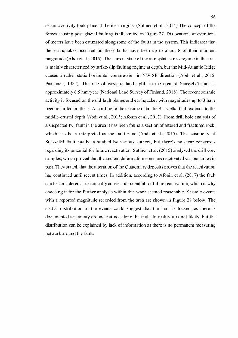
56
seismic activity took place at the ice-margins. (Sutinen et al., 2014) The concept of the
forces causing post-glacial faulting is illustrated in Figure 27. Dislocations of even tens
of meters have been estimated along some of the faults in the system. This indicates that
the earthquakes occurred on these faults have been up to about 8 of their moment
magnitude (Abdi et al., 2015). The current state of the intra-plate stress regime in the area
is mainly characterized by strike-slip faulting regime at depth, but the Mid-Atlantic Ridge
causes a rather static horizontal compression in NW-SE direction (Abdi et al., 2015,
Paananen, 1987). The rate of isostatic land uplift in the area of Suasselkä fault is
approximately 6.5 mm/year (National Land Survey of Finland, 2018). The recent seismic
activity is focused on the old fault planes and earthquakes with magnitudes up to 3 have
been recorded on these. According to the seismic data, the Suasselkä fault extends to the
middle-crustal depth (Abdi et al., 2015; Afonin et al., 2017). From drill hole analysis of
a suspected PG fault in the area it has been found a section of altered and fractured rock,
which has been interpreted as the fault zone (Abdi et al., 2015). The seismicity of
Suasselkä fault has been studied by various authors, but there’s no clear consensus
regarding its potential for future reactivation. Sutinen et al. (2015) analysed the drill core
samples, which proved that the ancient deformation zone has reactivated various times in
past. They stated, that the alteration of the Quaternary deposits proves that the reactivation
has continued until recent times. In addition, according to Afonin et al. (2017) the fault
can be considered as seismically active and potential for future reactivation, which is why
choosing it for the further analysis within this work seemed reasonable. Seismic events
with a reported magnitude recorded from the area are shown in Figure 28 below. The
spatial distribution of the events could suggest that the fault is locked, as there is
documented seismicity around but not along the fault. In reality it is not likely, but the
distribution can be explained by lack of information as there is no permanent measuring
network around the fault.
57
Figure 28 Suasselkä post-glacial fault and the seismic events reported nearby the fault
from 1842 onwards (the 1842 event of magnitude 3.2, the largest event reported in the
proximity of the Suasselkä fault, being the southmost event on 25th meridian east).
Seismic events from FENCAT EQ-search tool (http://www.seismo.helsinki.fi/EQ-
search/query.php) of the Institute of Seismology of the University of Helsinki.
The Suasselkä fault is the longest postglacial fault in Finland, with the total surface
rupture length of approximately 47 km. A significant electromagnetic anomaly in the NE
suggests that the fault thrusts from SE with a strike of 35 - 50. Surface signatures found
are numerous and differently oriented, scarp varying between 0 and 3 m, though some
authors suggested the maximum length to be up to 70 km, maximum scarp height being
even 5 m (Afonin et al., 2017; Abdi et al., 2015; Paananen, 1987). It can be assumed that
the fault has caused an earthquake with magnitude close to 7 (Sutinen et al., 2014). The
origin of the structure is likely to be even older than postglacial, especially on its eastern
end, as the magnetic measurements have indicated anomalies also of the
Palaeoproterozoic bedrock along the fault scarp. Previous studies have indicated two sets
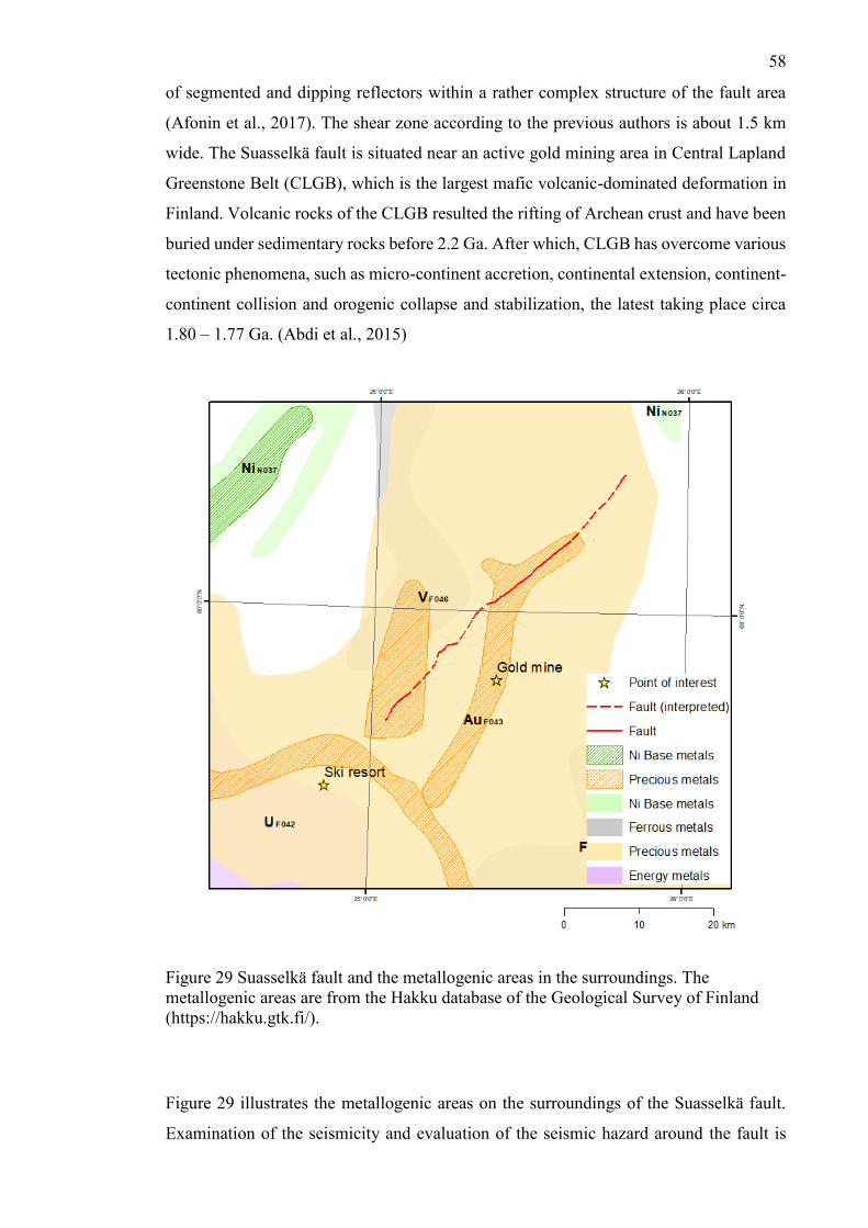
58
of segmented and dipping reflectors within a rather complex structure of the fault area
(Afonin et al., 2017). The shear zone according to the previous authors is about 1.5 km
wide. The Suasselkä fault is situated near an active gold mining area in Central Lapland
Greenstone Belt (CLGB), which is the largest mafic volcanic-dominated deformation in
Finland. Volcanic rocks of the CLGB resulted the rifting of Archean crust and have been
buried under sedimentary rocks before 2.2 Ga. After which, CLGB has overcome various
tectonic phenomena, such as micro-continent accretion, continental extension, continent-
continent collision and orogenic collapse and stabilization, the latest taking place circa
1.80 – 1.77 Ga. (Abdi et al., 2015)
Figure 29 Suasselkä fault and the metallogenic areas in the surroundings. The
metallogenic areas are from the Hakku database of the Geological Survey of Finland
(https://hakku.gtk.fi/).
Figure 29 illustrates the metallogenic areas on the surroundings of the Suasselkä fault.
Examination of the seismicity and evaluation of the seismic hazard around the fault is
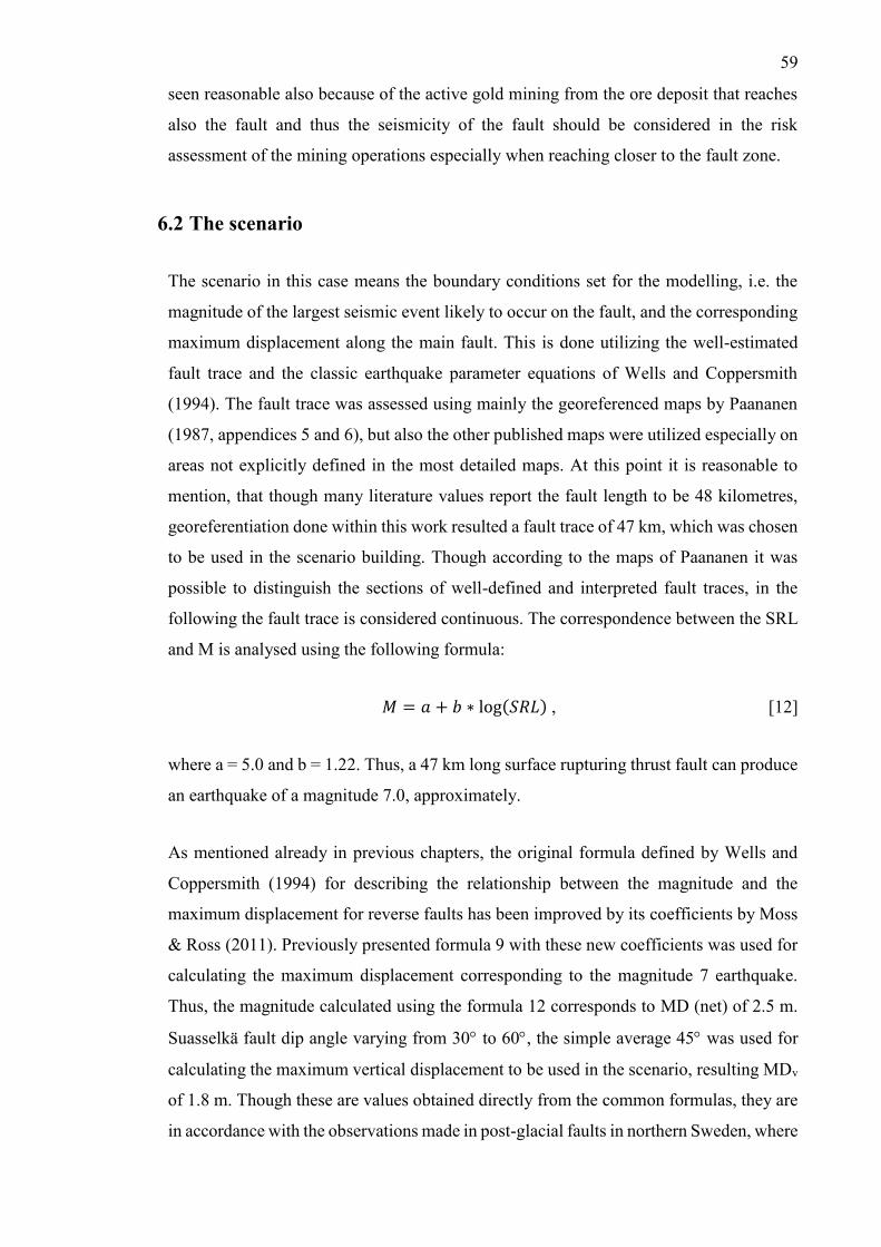
59
seen reasonable also because of the active gold mining from the ore deposit that reaches
also the fault and thus the seismicity of the fault should be considered in the risk
assessment of the mining operations especially when reaching closer to the fault zone.
6.2 The scenario
The scenario in this case means the boundary conditions set for the modelling, i.e. the
magnitude of the largest seismic event likely to occur on the fault, and the corresponding
maximum displacement along the main fault. This is done utilizing the well-estimated
fault trace and the classic earthquake parameter equations of Wells and Coppersmith
(1994). The fault trace was assessed using mainly the georeferenced maps by Paananen
(1987, appendices 5 and 6), but also the other published maps were utilized especially on
areas not explicitly defined in the most detailed maps. At this point it is reasonable to
mention, that though many literature values report the fault length to be 48 kilometres,
georeferentiation done within this work resulted a fault trace of 47 km, which was chosen
to be used in the scenario building. Though according to the maps of Paananen it was
possible to distinguish the sections of well-defined and interpreted fault traces, in the
following the fault trace is considered continuous. The correspondence between the SRL
and M is analysed using the following formula:
𝑀 = 𝑎 + 𝑏 ∗ log(𝑆𝑅𝐿) , [12]
where a = 5.0 and b = 1.22. Thus, a 47 km long surface rupturing thrust fault can produce
an earthquake of a magnitude 7.0, approximately.
As mentioned already in previous chapters, the original formula defined by Wells and
Coppersmith (1994) for describing the relationship between the magnitude and the
maximum displacement for reverse faults has been improved by its coefficients by Moss
& Ross (2011). Previously presented formula 9 with these new coefficients was used for
calculating the maximum displacement corresponding to the magnitude 7 earthquake.
Thus, the magnitude calculated using the formula 12 corresponds to MD (net) of 2.5 m.
Suasselkä fault dip angle varying from 30 to 60, the simple average 45 was used for
calculating the maximum vertical displacement to be used in the scenario, resulting MDv
of 1.8 m. Though these are values obtained directly from the common formulas, they are
in accordance with the observations made in post-glacial faults in northern Sweden, where
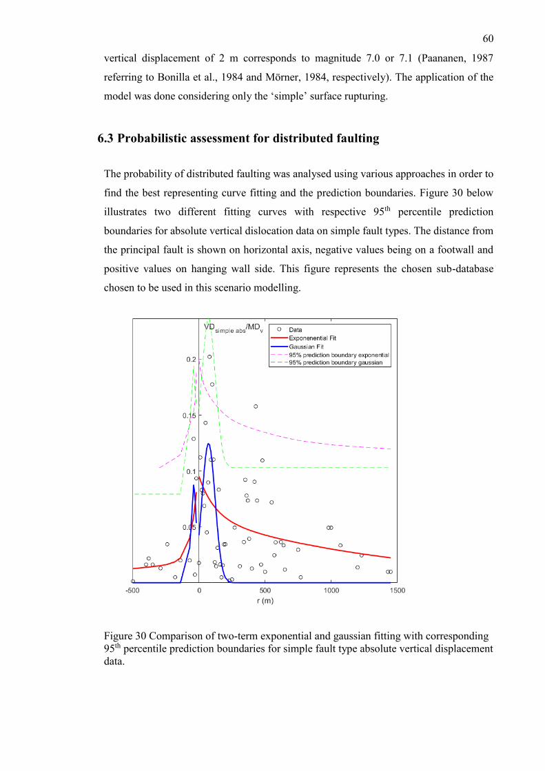
60
vertical displacement of 2 m corresponds to magnitude 7.0 or 7.1 (Paananen, 1987
referring to Bonilla et al., 1984 and Mörner, 1984, respectively). The application of the
model was done considering only the ‘simple’ surface rupturing.
6.3 Probabilistic assessment for distributed faulting
The probability of distributed faulting was analysed using various approaches in order to
find the best representing curve fitting and the prediction boundaries. Figure 30 below
illustrates two different fitting curves with respective 95th percentile prediction
boundaries for absolute vertical dislocation data on simple fault types. The distance from
the principal fault is shown on horizontal axis, negative values being on a footwall and
positive values on hanging wall side. This figure represents the chosen sub-database
chosen to be used in this scenario modelling.
Figure 30 Comparison of two-term exponential and gaussian fitting with corresponding
95th percentile prediction boundaries for simple fault type absolute vertical displacement
data.
61
The following calculations are done for the scenario event representing the biggest
expectable event on Suasselkä fault using the parameters described previously. Figure 31
below illustrates the probability of DF displacement in various distances from the
principal fault shown by the survival functions for both hanging wall and footwall sides.
It can be seen that the displacements of larger displacements on footwall are concentrated
to a relatively narrower area than on the hanging wall.
Figure 31 Probability of the occurrence of distributed faulting plotted against the
distance from the principal fault trace
The absolute and conditional probabilities of exceedance of VDL are plotted in distances
of 6, 10, 100 and 500 m from the main fault. The 6 m distance is the limit the model
considers for dividing the distributed faulting from the principal fault rupturing. The other
distances are chosen arbitrarily. Figure 32 below illustrates the absolute probabilities of
exceedance for the chosen distances from the PF, Figure 33 instead the conditional ones.
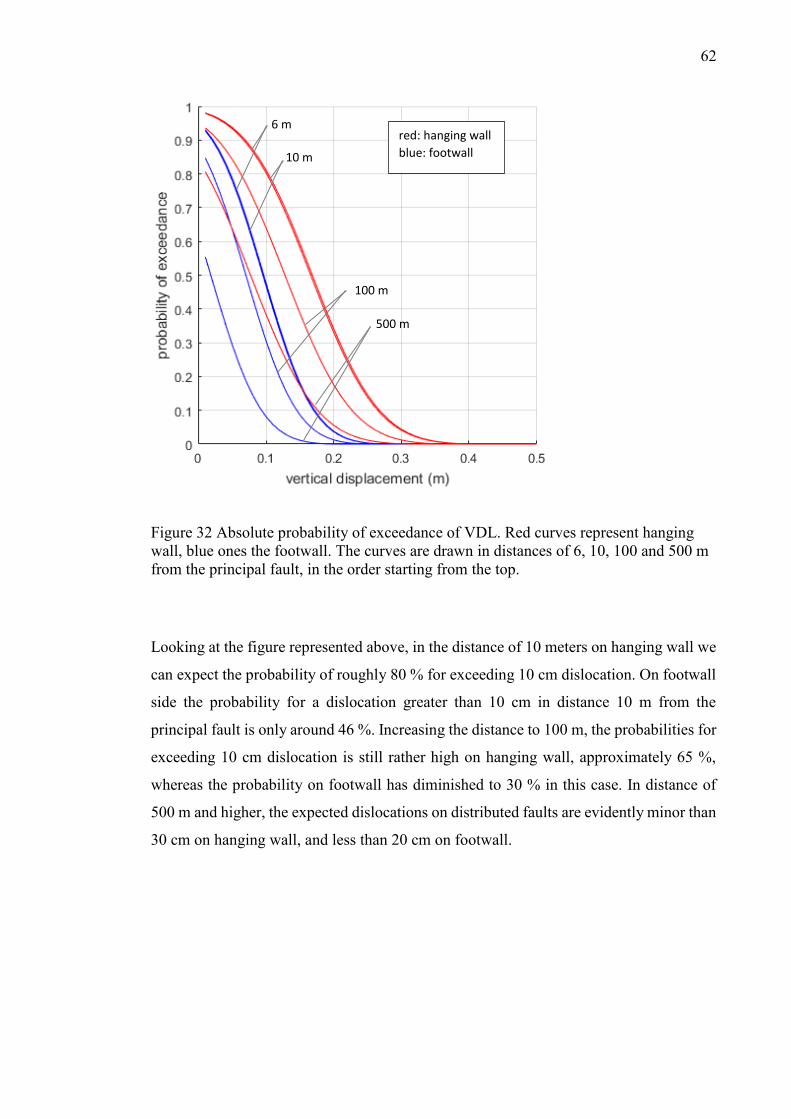
62
Figure 32 Absolute probability of exceedance of VDL. Red curves represent hanging
wall, blue ones the footwall. The curves are drawn in distances of 6, 10, 100 and 500 m
from the principal fault, in the order starting from the top.
Looking at the figure represented above, in the distance of 10 meters on hanging wall we
can expect the probability of roughly 80 % for exceeding 10 cm dislocation. On footwall
side the probability for a dislocation greater than 10 cm in distance 10 m from the
principal fault is only around 46 %. Increasing the distance to 100 m, the probabilities for
exceeding 10 cm dislocation is still rather high on hanging wall, approximately 65 %,
whereas the probability on footwall has diminished to 30 % in this case. In distance of
500 m and higher, the expected dislocations on distributed faults are evidently minor than
30 cm on hanging wall, and less than 20 cm on footwall.
red: hanging wall
blue: footwall
6 m
10 m
100 m
500 m
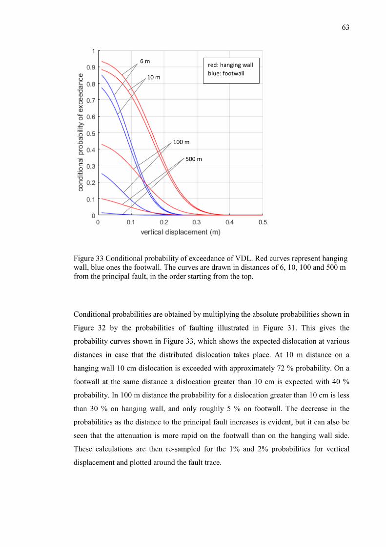
63
Figure 33 Conditional probability of exceedance of VDL. Red curves represent hanging
wall, blue ones the footwall. The curves are drawn in distances of 6, 10, 100 and 500 m
from the principal fault, in the order starting from the top.
Conditional probabilities are obtained by multiplying the absolute probabilities shown in
Figure 32 by the probabilities of faulting illustrated in Figure 31. This gives the
probability curves shown in Figure 33, which shows the expected dislocation at various
distances in case that the distributed dislocation takes place. At 10 m distance on a
hanging wall 10 cm dislocation is exceeded with approximately 72 % probability. On a
footwall at the same distance a dislocation greater than 10 cm is expected with 40 %
probability. In 100 m distance the probability for a dislocation greater than 10 cm is less
than 30 % on hanging wall, and only roughly 5 % on footwall. The decrease in the
probabilities as the distance to the principal fault increases is evident, but it can also be
seen that the attenuation is more rapid on the footwall than on the hanging wall side.
These calculations are then re-sampled for the 1% and 2% probabilities for vertical
displacement and plotted around the fault trace.
red: hanging wall
blue: footwall
6 m
10 m
100 m
500 m
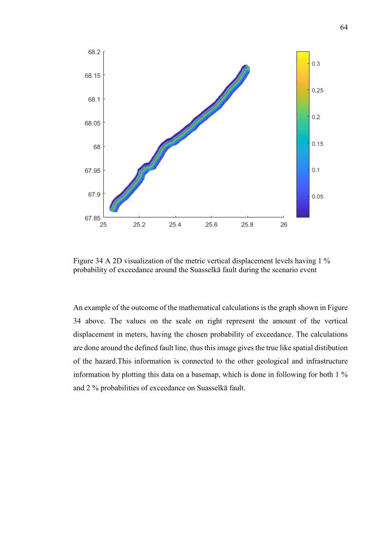
64
Figure 34 A 2D visualization of the metric vertical displacement levels having 1 %
probability of exceedance around the Suasselkä fault during the scenario event
An example of the outcome of the mathematical calculations is the graph shown in Figure
34 above. The values on the scale on right represent the amount of the vertical
displacement in meters, having the chosen probability of exceedance. The calculations
are done around the defined fault line, thus this image gives the true like spatial distibution
of the hazard.This information is connected to the other geological and infrastructure
information by plotting this data on a basemap, which is done in following for both 1 %
and 2 % probabilities of exceedance on Suasselkä fault.
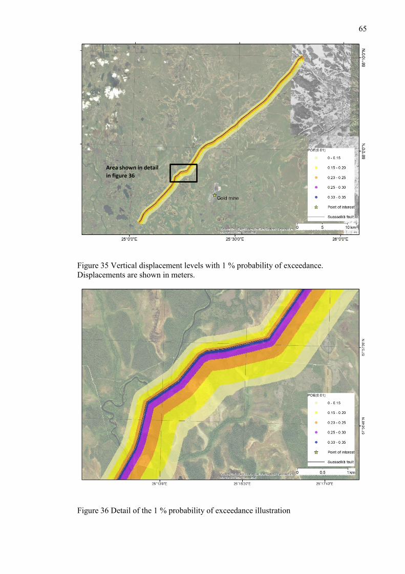
65
Figure 35 Vertical displacement levels with 1 % probability of exceedance.
Displacements are shown in meters.
Figure 36 Detail of the 1 % probability of exceedance illustration
Area shown in detail
in figure 36
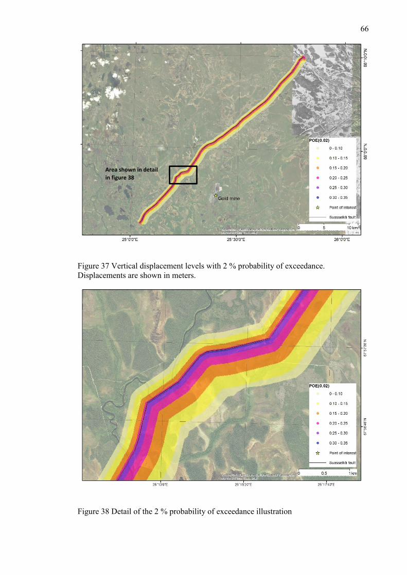
66
Figure 37 Vertical displacement levels with 2 % probability of exceedance.
Displacements are shown in meters.
Figure 38 Detail of the 2 % probability of exceedance illustration
Area shown in detail
in figure 38

67
The alternative end results of the modelling are shown in the maps in Figures 35 and 37.
They illustrate 1 % and 2 % probabilities of surface rupturing in the vicinity of the mapped
fault trace in case of a seismic event chosen in the modelling. Figures 36 and 38 show the
same area in more detail, with the probability of exceedance of 1 % and 2 %, respectively.
This type of modelling helps in estimation of the seismic risk in specific locations around
any active fault, and supports the decision making when placing the critical operations on
these areas. Figures 35 and 37 are provided larger in the appendices 2 and 3, respectively.
68
7 DISCUSSION
Geophysics combines two rather different disciplines by nature, bringing into a strongly
empirical science of geology the theorems and tools of physics. Thus, the results of
geophysical analysis such as this need to be understood as a union of a primarily
theoretical approach of physics, and the geological practise where the scientific
intelligence rises from enlightened interpretation of the natural environment. When the
work is done respecting the dual nature of the science of geophysics, it can provide greater
understanding on the natural phenomena.
The sources of uncertainties are numerous in this type of analysis. The inaccuracies within
creating a model like this are both epistemic and aleatory by nature, and they rise from
various sources. They can be categorized by their origin to the error sources emerging
from the original field work, data gathering and data analysis. In general, the prevalent
conditions while field working and the used methods and tools impact on the general
measurement accuracy, and the chosen measurement logic and geometry cause the
systematic margin of error, whereas the operator related errors usually result single, non-
systematic uncertainties in the data. However, this part is not considered in this work.
When working with datasets published by various study groups, the challenge lays in
uniting the miscellaneous types of data and the maps of various scales. In the model there
are possible uncertainties rising from the data handling and the analysis. These have been
discussed already in previous chapters together with the methodological choices done
during the work, and their possible impact on the overall trustworthiness of the model.
The work done here was rather extensive in sense of methodological development, and a
lot of effort was done for finding the selections leading to the most reliable end result.
The model created using the absolute vertical displacement of distributed faulting
normalized by the maximum vertical dislocation along the main fault seems to contain
the minimum uncertainty possible. As it has been shown here, the exclusion of the
complex types of secondary structures makes the analysis more precise and more suitable
on the analysis on the areas where the geology is well known. However, when estimating
the overall hazard also in areas where not detailed geological survey is done, it might be
better to use the probability distribution of all types of secondary ruptures.
69
During the work there was a continuous discussion between the theoretical ideal and the
extend of the database, and several selections had to be done due to the incompleteness
of the empirical data. For example, since defining the net slip along the secondary fault
ruptures was not that straightforward as for the PF for the reasons explained earlier, the
fitting of the probability distribution curves obtained using the data of net slip was not as
good as for the pure vertical slip data, even though the theoretical hypothesis suggested
the net slip being more representative value. I also noticed that even if there were only
few cases with secondary surface rupturing that demonstrated normal slipping movement
near the surface, their impact was visible in the fitting when included in the analysis as
absolute values. Including this absolute vertical slip data in the database is reasonable
because not always the movement on the secondary fault is identical to the dislocation on
the PF anyway, as all types of oblique slipping were reported in the studied cases. The
only reason why the normal slipping was separated in the first place was purely technical,
as they were first reported negative in the database and thus they were easily cancelled
out.
According to Wells & Coppersmith (1994), when applying the model into a certain field
environment, the most significant sources of error are related to the empirical probability
of the surface rupturing, the lognormal distribution of the dislocation along the principal
fault used as a normalization factor, and the spatial dependence of the normalized
dislocation on the secondary fault ruptures. Depending on the basis by which the expected
maximum magnitude is estimated, the work requires anyhow a good knowledge of the
fault system setting and the maximum length of the fault active and capable of producing
an earthquake. These are always a pair, and the assumption of given magnitude being the
maximum is valid only when also the input parameter of the calculation, i.e. the SRL, can
be considered as a maximum value. The model itself (with all the in-built uncertainties)
cannot be taken as one detailed truth, but the modelling always requires the interpretation
of the local conditions. The uncertainties in applicating the model to the natural
environment emerge also from the accuracy of the interpretation of the possible fault
trace.
The problem regarding the varying data of the previous authors is not new, and also Wells
& Coppersmith (1994) mentioned the same problem: the goal of a research like this is to
recognise the most accurate value for each parameter. This, however, requires intensive
familiarization with the reference material, which might be plenty. The scientific

70
community is self-controlling, but I believe the discussion goes rarely up to initial
database and measurement logics. The sources of uncertainties regarding the reported
surface rupturing listed by Wells & Coppersmith (1994) remain valid also today. For a
more reliable analysis, a standardized method for initial field work could diminish the
uncertainty of the further calculations and increase the accuracy of the future hazard
analysis. The dataset of this work is rather small, and thus its ability to represent
comprehensively all the thrust earthquakes can be discussed. However, the database was
kept small in order to maintain the quality: only the well-studied events with well
documented reference material were included in the analysis. It is not reasonable to
increase the database by digging further in history, as the faults are likely exposed to post-
seismic movements. Thus, the only way to improve the model is to fill it up with well-
studied future events. In the end, it needs to be accepted that predicting a highly complex
spatial-temporal phenomenon, such as an earthquake, using simple parameters like
magnitude for representing the total seismic energy released during the event, cannot
arrive to the highest certainty. However, using the high quality empirical data it was
possible to create a model that can be used for the assessment of the seismic risk needed
when evaluation of positioning the infrastructures and operations, which was the intention
of this work.
71
8 CONCLUSIONS
Earthquakes cannot be predicted explicitly, but the seismic hazard can be modelled quite
efficiently utilizing the knowledge provided by the previous seismic events. The
empirical data of the well-studied earthquakes can be brought together to a collected
database, and the generalized data can be used for obtaining the parameters used in the
calculation of the probabilities of surface dislocations and further in modelling this hazard
to other seismic environments. This work was concentrated on the seismic hazard related
to earthquakes on reverse tectonic setting. The detailed analysis of the distributed fault
rupturing during reverse faulting earthquakes has been missing from the scientific
discussion.
This work started by gathering data from 11 historical earthquakes listing all the provided
information of the surface faulting both on the principal fault and the distributed faults.
The spatial distribution of the distributed surface rupturing was done by georeferencing
the maps published by the researchers that studied the area right after the seismic event.
The methodological approach used in this phase was developed during the work, and it
seems to provide more detailed information than for example the grid system used by
other authors previously. Once the database was completed for every event, the data was
generalized by normalizing the displacement values to the normalization parameters
obtained from the principal fault dislocation. The generalized data was used for
calculating the probability of occurrence of distributed surface rupturing, and the
probability of certain dislocation levels within these faults. The analysis of the probability
of distributed surface rupturing was done separately for ‘simple’ scarp types, and with
considering also the more complex geological setting resulting secondary surface faulting
strictly related to the special sub-surface structure of the faulting zone (‘all’). The
probability of the occurrence of the distributed surface rupturing was obtained from the
attenuation functions drawn using a known fitting curve best representing the empirical
data. Statistically the most robust approach for distributed surface faulting was found
using the absolute vertical dislocation data normalized by the maximum vertical
dislocation along the principal fault. For the further modelling, only the ‘simple’ scarp
type data was considered.
The computational model created here illustrates the probabilities for distributed surface
rupturing using a grid of 10 x 10 m, calculating the probability for each grid point
72
separately. The model uses the scenario approach, meaning that it describes the situation
within an earthquake during which the fault ruptures along its total length. The input
values of the model are those calculated in the previous phases of the work, as well as the
geometry of a chosen fault around which the seismic hazard is modelled. The
computational model provides an illustration of different hazard levels that can be
transformed on a base map for the location specific analysis. In the last phase of this work,
the created model was utilized in the analysis of the seismic hazard around the Suasselkä
post-glacial fault in Northern Finland. The activity of the fault is under discussion, but
there are some important activities around the fault and thus it was seen reasonable to
model the seismic hazard on that area. The model results illustrations of the different
hazard levels on a base map around the Suasselkä fault trace that may help in location
specific risk assessment.
The key limitation in the model as such is that it does not consider the temporal or spatial
variation of the principal faulting but is limited to the “maximum” with the scenario
approach. In the future, the model could be developed further by including the temporal
changes, which would increase the options of the possible outcomes of the modelling.
The reliability of the modelling increases as the source database is enhanced by adding
data of other well-studied seismic events. Implementing the model to other types of fault
settings would require gathering a similar type of database of normal and strike-slip
faulting earthquakes and using those for obtaining the required input parameters for the
modelling. This work concentrated on finding statistically the most robust approach and
tried to explain the choices made. Thus, it is not necessary to follow every single step
described here when building up the databases for normal faulting and strike-slip faulting
earthquakes, or when updating the one existing for the reverse fault earthquakes. This
model has shown its potential in location specific analysis of seismic hazard, but it can
always improve and become more accurate.
73
REFERENCES
Abdi, A., Heinonen, S., Juhlin, C. & Karinen T., 2015. Constraints on the geometry of
the Suasselkä post-glacial fault, northern Finland, based on reflection seismic imaging.
Tectonophysics, 649, pp. 130–138.
Afonin, N., Kozlovskaya, E., Kukkonen, I. & DAFNE/FINLAND Working Group, 2017.
Structure of the Suasselkä postglacial fault in northern Finland obtained by analysis of
local events and ambient seismic noise. Solid Earth, 8, pp. 531-544.
https://doi.org/10.5194/se-8-531-2017
Angelier, J., Lee, J. C., Chu, H. T. & Hu, J. C., 2003. Reconstruction of fault slip of the
September 21st, 1999, Taiwan earthquake in the asphalted surface of a car park, and co-
seismic slip partitioning. Journal of Structural Geology, 25, pp. 345–350.
Baker, J.W., 2008. An Introduction to Probabilistic Seismic Hazard Analysis (PSHA).
Report. Available at: https://www.researchgate.net/publication/237770309_An
_Introduction_to_Probabilistic_Seismic_Hazard_Analysis_PSHA.
Bilham, R. & Yu, T. T., 2000. The morphology of thrust faulting in the 21 September
1999, Chichi, Taiwan earthquake, Journal of Asian Earth Sciences, 18, pp. 351–367.
Boncio, P., Liberi, F., Caldarella, M. & Nurminen F.-C., 2018. Width of surface rupture
zone for thrust earthquakes: implications for earthquake fault zoning. Natural Hazards
and Earth System Sciences, 18, pp 241-256. https://doi.org/10.5194/nhess-18-241-2018
Bowman, J. R. & Barlow, B. C., 1991. Surveys of the Fault Scarp of the 1986 Marryat
Creek, South Australia, Earthquake, [Australian] Bureau of Mineral Resources, Geology
and Geophysics, Canberra, AU, BMR Record 1991/190.
Caldarella, M., 2016. Caratteristiche delle zone di fagliazione cosismica in superficie di
terremoti inversi: implicazioni sulla pericolosità per faglie attive e capaci. MSc thesis.
The ‘G. d’Annunzio’ University, Department of Engineering and Geology (in Italian with
English abstract)
74
Central Geological Survey, MOEA, 2017. [URL-document] Available at:
http://gis.moeacgs.gov.tw/gwh/gsb97-1/sys8/index.cfm [read October 2017].
Chang, J. C. & Yang, G. S., 2004. Deformation and occurrence of the Che-lung-pu Fault
from geomorphic evidence. Quaternary International, 115–116, pp. 177–188.
Chen, C. H., Chou, H. S., Yang, C. Y., Shieh, B. J. & Kao, Y. H., 2003. Chelungpu fault
inflicted damages of pile foundations on FWY rout 3 and Fault zoning regulations in
Taiwan, in: Proceedings of the JSCE/EqTAP Workshop on Seismic Fault-induced
Failures, Tokyo, Japan, 22 February 2003, pp. 1–19.
Chen, G.H., Xu, X.W., Zheng, R.Z., Yu, G.H., Li, F., Li, C.X., Wen, X.Z., He, Y.L., Ye,
Y.Q., Chen, X.C., and Wang, Z.C., 2008. Quantitative analysis of the co-seismic surface
rupture of the 2008Wenchuan earthquake, Sichuan, China along the Beichuan-Yingxiu
Fault. Seismology and Geology, 30 (3), pp. 723–738. (in Chinese with English abstract)
Coppersmith K.J. & Youngs R.R., 1990. Probabilistic seismic-hazard analysis using
expert opinion – An example from the Pacific Northwest. Geological Society of America.
Reviews in Engineering Geology, 8, pp. 29-46.
Coppersmith K.J. & Youngs R.R., 2000. Data needs for probabilistic fault displacement
hazard analysis. Journal of Geodynamics, 29, pp. 329-343.
Cornell, C.A., 1968. Engineering seismic risk analysis. Bulletin of the Seismological
Society of America, 58, pp. 1583-1606.
Cornell, C.A., 1971. Probabilistic analysis of damage to the structures under seismic
loads. In Howells, D.A., Haigh, I.P. & Taylor, C. (eds.) Dynamic Waves in Civil
Engineering. John Wiley, London.
Crone, A. J., Machette, M. N., & Bowman, J. R., 1992. Geologic investigations of the
1988 Tennant Creek, Australia, earthquakes – implications for paleoseismicity in stable
continental regions. US Geological Survey Bulletin 2032-A.
Dong S., Zhang Y., Wu Z., Yang, N., Ma, Y., Shi, W., Chen, Z., Long, C. & An, M.,
2008a. Surface rupture and co-seismic displacement produced by the Ms 8.0 Wenchuan
75
earthquake of May 12th, 2008, Sichuan, China: eastwards growth of the Qinghai-Tibet
Plateau. Acta Geologica Sinica, 82 (5), pp. 938–948.
Dong, S., Han, Z. & An, Y., 2008b. Surface deformation at the epicentre of the May 12,
2008 Wenchuan M8 Earthquake, at Yingxiu Town of Sichuan Province, China. Science
in China Series E: Technological Sciences, 51, pp. 154–163.
https://doi.org/10.1007/s11431-008-6007-0
Faccioli, E., Anastasopoulos, I., Gazetas, G., Callerio, A. & Paolucci, R., 2008. Fault
rupture–foundation interaction: selected case histories. Bulletin of Earthquake
Engineering, 6, pp. 557–583.
Fredrich, J., McCaffrey, R. & Denham, D., 1988. Source parameters of seven large
Australian earthquakes determined by body waveform inversion, Geophysical Journal+,
95, pp. 1–13.
Haessler, H., Deschamps, A., Dufumier, H., Fuenzalida, H. & Cisternas, A., 1992. The
rupture process of the Armenian earthquake from broad-band teleseismic body wave
records, Geophysical Journal International, 109, pp. 151–161.
Huang, C., Chan Y.-C., Hu, J.-C., Angelier, J. & Lee, J.-C., 2008. Detailed surface co-
seismic displacement of the 1999 Chi-Chi earthquake in western Taiwan and implication
of fault geometry in the shallow subsurface. Journal of Structural Geology, 30, pp. 1167–
1176.
Huang, W.J., Chen, Z.Y., Liu, S.Y., Lin, Y.H., Lin, C.W. & Chang, H.C., 2000. Surface
deformation models of the 1999 Chi–Chi earthquake between Tachiachi and
Toupienkengchi, central Taiwan, Special Issue for the Chi-Chi Earthquake, 1999, Central
Geological Survey, MOEA, Taipei, Taiwan, Special Publication, 12, pp. 63–87. (in
Chinese with English abstract).
Huang, W.J., 2006. Deformation at the Leading Edge of Thrust Faults. PhD dissertation,
Purdue University, West Lafayette, Indiana.

76
Ishimura, D., Okada, S., Niwa, Y., and Toda, S., 2015. The surface rupture of the 22
November 2014 Nagano-ken-hokubu earthquake (Mw 6.2), along the Kamishiro fault,
Japan, Active Fault Research, 43, pp. 95–108. (in Japanese with English abstract)
Kamb, B., Silver, L.T., Abrams M.J., Carter B.A., Jordan T.H. & Minster, J.B., 1971.
Pattern of faulting and nature of fault movement in the San Fernando earthquake, in: The
San Fernando, California, earthquake of February 9, 1971, US Geological Survey,
Washington, Professional Paper 733, pp. 41–54.
Kaneda, H., Nakata, T., Tsutsumi, H., Kondo, H., Sugito, N., Awata, Y., Akhtar, S.S.,
Majid, A., Khattak, W., Awan, A.A., Yeats, R.S., Hussain, A., Ashraf, M., Wesnousky,
S.G. & Kausar, A.B., 2008. Surface rupture of the 2005 Kashmir, Pakistan, Earthquake
and its active tectonic implications, Bulletin of the Seismological Society of America, 98,
pp. 521–557.
Kawashima, K., 2002. Damage of bridges resulting from fault rupture in the 1999 Kocaeli
and Dunce, Turkey earthquakes and the 1999 Chi-Chi, Taiwan earthquake. Structural
Eng./Earthquake Eng., JSCE, 19 (2), pp. 179–197.
Kelson, K.I., Kang, K.-H., Page, W.D., Lee, C.-T. & Cluff, L.S., 2001. Representative
styles of deformation along the Chelungpu fault from the 1999 Chi-Chi (Taiwan)
Earthquake: Geomorphic characteristics and responses of man-made structures. Bulletin
of the Seismological Society of America, 91 (5), pp. 930-952.
Kelson, K.I., Koehler, R.D., Kang, K.-H., Bray, J.D. & Cluff, L.S., 2003. Surface
deformation produced by the 1999 Chichi (Taiwan) earthquake and interactions with built
structures. William Lettis & Associates, Inc., Walnut Creek, CA, Final Technical Report
submitted to US Geological Survey, Award No. 01HQ-GR-0122, 21.
Konagai, K., Hori, M., Meguro, K., Koseki, J., Matsushima, T., Johansson, J. & Murata,
O., 2006. Key Points for Rational Design for Civil Infrastructures near Seismic Faults
Reflecting Soil-Structure Interaction Features, Japan Geotechnical Society, Tokyo, JP,
Report of JSPS research project, grant-in-aid for scientific research (A) Project No.
16208048, 146.
77
Kukkonen, I., Olesen, O. & Ask, M.V.S., 2010. PFDP Working Group. Postglacial faults
in Fennoscandia: targets for scientific drilling. Journal of geological society of Sweden,
132, pp. 71–81.
Kumahara, Y. & Nakata, T., 2007. Recognition of active faults generating the 2005
Pakistan earthquake based on interpretation of the CORONA satellite photographs. E-
journal GEO, 2, pp. 72–85. (in Japanese with English abstract)
Lee, G.C. & Loh, C.H. (Eds), 2000. The Chi-Chi, Taiwan Earthquake of September 21,
1999: Reconnaissance Report. Multidisciplinary Center for Earthquake Engineering
Research, Technical Report MCEER-00-0003.
Lee, J.C., Chen, Y.G., Sieh, K., Mueller, K., Chen, W.S., Chu, H.T., Chan, Y.C., Rubin,
C. & Yeats, R., 2001. A vertical exposure of the 1999 surface rupture of the Chelungpu
Fault at Wufeng, Western Taiwan: structural and paleoseismic implications for an active
thrust fault. Bulletin of the Seismological Society of America, 91, (5), pp. 914–929.
Lee, J.C. & Chan, Y.C., 2007. Structure of the 1999 Chi-Chi earthquake rupture and
interaction of thrust faults in the active fold belt of western Taiwan, Journal of Asian
Earth Sciences, 31, pp. 226–239.
Lee, Y.H., Hsieh, M.L., Lu, S.D., Shih, T.S., Wu, W.Y., Sugiyama, Y., Azuma, T. &
Kariya, Y., 2003. Slip vectors of the surface rupture of the 1999 Chi-Chi earthquake,
western Taiwan, Journal of Structural Geology, 25, pp. 1917–1931.
Lee, Y. H., Wu, K. C., Rau, R. J., Chen, H. C., Lo, W. & Cheng, K. C., 2010. Revealing
coseismic displacements and the deformation zones of the 1999 Chi-Chi earthquake in
the Tsaotung area, central Taiwan, using digital cadastral data, Journal of Geophysical
Research, 115 (B03419). https://doi.org/10.1029/2009JB006397
Lettis, W.R., Wells, D.L. & Baldwin, J. N., 1997. Empirical observations regarding
reverse earthquakes, blind thrust faults, and quaternary deformation: are blind thrust
faults truly blind?, Bulletin of the Seismological Society of America, 87, pp. 1171–1198.
78
Lin, A., Sano, M., Yan, B., and Wang, M., 2015. Co-seismic surface ruptures produced
by the 2014 Mw 6.2 Nagano earthquake, along the Itoigawa–Shizuoka tectonic line,
central Japan. Tectonophysics, 656, pp. 142–153.
Lin, W. H., 2000. On surface deformations from the Chi-Chi earthquake in the Shihkang
and Chutzekeng areas, Special Issue for the Chi-Chi Earthquake, 1999. Central
Geological Survey, MOEA, Taipei, Taiwan, Special Publication, 12, pp. 1–17. (in
Chinese with English abstract)
Liu-Zeng, J., Zhang, Z., Wen, L., Tapponnier, P., Sun, J., Xing, X., Hu, G., Xu, Q., Zeng,
L., Ding, L., Ji, C., Hudnut, K.W. & van der Woerd, J., 2009. Co-seismic ruptures of the
12 May 2008, Ms 8.0 Wenchuan earthquake, Sichuan: east–west crustal shortening on
oblique, parallel thrusts along the eastern edge of Tibet. Earth and Planetary Science
Letters, 286, pp. 355–370.
Liu-Zeng, J., Sun, J., Zhang, Z., Wen, L., Xing, X., Hu, G. & Xu, Q., 2010. Detailed
mapping of surface rupture of theWenchuan Ms 8.0 earthquake near Hongkou and
seismotectonic implications. Quaternary Sciences, 30, pp. 1–29. (in Chinese with English
abstract)
Liu-Zeng, J., Sun, J., Wang, P., Hudnut, K.W., Ji, C., Zhang, Z., Xu, Q. & Wen, L., 2012.
Surface ruptures on the transverse Xiaoyudong fault: a significant segment boundary
breached during the 2008 Wenchuan earthquake, China. Tectonophysics, 580, pp. 218–
241.
Machette, M. N., Crone, A. J., & Bowman, J. R., 1993. Geologic investigations of the
1986 Marryat Creek, Australia, earthquakes – implications for paleoseismicity in stable
continental regions. US Geological Survey Bulletin, 2032-B.
McCaffrey, R., 1989. Teleseismic investigation of the January 22, 1988 Tennant Creek,
Australia, earthquakes, Geophysical Research Letters, 16, pp. 413–416.
Meghraoui, M., Jaegy, R., Lammali, K., & Albarède, F., 1988. Late Holocene earthquake
sequences on the El Asnam (Algeria) thrust fault. Earth Planet. Science Letters, 90, pp.
187–203.

79
Moss R.E.S. & Ross Z.E., 2011. Probabilistic Fault Displacement Hazard Analysis for
Reverse Faults. Bulletin of the Seismological Society of America, 101 (4), pp. 1542-1553.
Mörner, N.A., 1984. Paleoseismicity and geodynamics in Sweden. Seismotectonics.
Tectonophysics 117, pp. 139-153.
National Land Survey of Finland. Land uplift [URL-document] Available at:
http://www.maanmittauslaitos.fi/en/research/interesting-topics/land-uplift [Read: March
2018]
Okada, S., Ishimura, D., Niwa, Y., and Toda, S., 2015. The first surface rupturing
earthquake in 20 years on a HERP active fault is not characteristic: the 2014 Mw 6.2
Nagano event along the northern Itoigawa–Shizuoka tectonic line. Seismological
Research Letters, 86, pp. 1–14.
Olesen, O., Blikra, L.H., Braathen, A., Dehls, J.F., Olsen, L., Rise, L., Roberts, D., Riis,
F., Faleide, J.I. & Anda, E., 2004. Neotectonic deformation in Norway and its
implications: a review. Norwegian Journal of Geology, 84, pp. 3–34.
Ota, Y., Huang, C. Y., Yuan, P. B., Sugiyama, Y., Lee, Y. H., Watanabe, M., Sawa, H.,
Yanagida, M., Sasaki, S., Suzuki, Y., Tang, H. S., Shu, U. T., Yang, S. Y., Hirouchi, D.,
& Taniguchi, K., 2001. Trenching study at the Tsautun Site on the central part of the
Chelungpu Fault, Taiwan, Journal of Geography, 110, pp. 698–707. (in Japanese with
English abstract)
Ota, Y., Watanabe, M., Suzuki, Y., Yanagida, M., Miyawaki, A. & Sawa, H., 2007a. Style
of the surface deformation by the 1999 Chichi earthquake at the central segment of
Chelungpu fault, Taiwan, with special reference to the presence of the main and
subsidiary faults and their progressive deformation in the Tsauton area, Journal of Asian
Earth Sciences, 31, pp. 214–225.
Ota, Y., Shishikura, M., Ichikawa, K., Watanabe, M., Yanagida, M., Tanaka, T., Sawa,
H., Yamaguchi, M., Lee, Y. H., Lu, S. T., Shih, T. S. & Amagasa, S., 2007b. Low-angle
reverse faulting during two earthquakes on the northern part of the Chelungpu fault,
deduced from the Fengyuan trench, Central Taiwan. Terrestrial, Atmospheric and
Oceanic Sciences, 18, pp. 55–66.
80
Paananen M., 1987. Venejärven, Ruostejärven, Suasseljän ja Pasmajärven
postglasiaalisten siirrosten geofysikaalinen tutkimus. Geological Survey of Finland,
Nuclear Waste Disposal Research, Report YST – 59. ISBN 951-690-294-4 (in Finnish
with English abstract)
Petersen M.D., Dawson T.E., Chen R., Cao T., Wills C.J., Schwartz D.P. & Frankel A.D.,
2011. Fault Displacement Hazard for Strike-Slip Faults. Bulletin of the Seismological
Society of America, 101 (2), pp. 805-825.
Philip, H. & Meghraoui, M., 1983. Structural analysis and interpretation of the surface
deformation of the El Asnam earthquake of October 10, 1980, Tectonics, 2, 17–49.
Philip, H., Rogozhin, E., Cisternas, A., Bousquet, J. C., Borisov, B., & Karakhanian, A.,
1992. The Armenian earthquake of 1988 December 7: faulting and folding, neotectonics
and palaeoseismicity. Geophysical Journal International, 110, pp. 141–158.
Rajendran, C. P., Rajendran, K., Unnikrishnan, K. R. & John, B., 1996. Palaeoseismic
indicators in the rupture zone of the 1993 Killari (Latur) earthquake, Current Science
India, 70 (5), pp. 385–390.
Rymer, M. J., Kendrick, K. J., Lienkaemper, J. J., & Clark, M. M., 1990. Surface rupture
on the Nunez fault during the Coalinga earthquake sequence, in: The Coalinga, California,
Earthquake of May 2, 1983. US Geological Survey Professional Paper 1487, pp. 299–
318.
Seeber, L., Ekstrom, G., Jain, S. K., Murty, C. V. R., Chandak, N. & Armbruster, J. G.,
1996. The 1993 Killari earthquake in central India: a new fault in Mesozoic basalt flows?.
Journal of Geophysical Research, 101 (B4), pp. 8543–8560.
https://doi.org/10.1029/95JB01865
Shin, T. C. & Teng, T. L., 2001. An overview of the 1999 Chi-Chi, Taiwan, Earthquake,
Bulletin of the Seismological Society of America, 91, pp. 895–913.
Sutinen, R., Hyvönen E. & Kukkonen, I., 2014. LiDAR detection of paleolandslides in
the vicinity of the Suasselkä postglacial fault, Finnish Lapland. International Journal of
Applied Earth Observation and Geoinformation 27, pp. 91-99.
81
US Geological Survey Staff, 1971. Surface faulting, in: The San Fernando, California,
earthquake of February 9, 1971. US Geological Survey, Washington, Professional Paper
733, pp. 55–76.
USGS, 2018. Earthquake Glossary. [URL-document] Available at:
https://earthquake.usgs.gov/learn/glossary/?term=fault [Read: March 2018]
Wang, H., Ran, Y, Chen, L., Shi, X., Liu, R. & Gomez, F., 2010. Determination of
horizontal shortening and amount of reverse-faulting from trenching across the surface
rupture of the 2008 Mw 7.9 Wenchuan earthquake, China. Tectonophysics, 491, pp. 10–
20.
Wells D.L. & Coppersmith K.J., 1994. New Empirical Relationship among Magnitude,
Rupture Length, Rupture Width, Rupture Area, and Surface Displacement. Bulletin of
the Seismological Society of America, 84 (4), pp. 974-1002.
Wells D.L. & Kulkarni V.S., 2014. Probabilistic Fault Displacement Hazard Analysis –
Sensitivity Analyses and Recommended Practices for Developing Design Fault
Displacements. Proceedings of the 10th National Conference in Earthquake Engineering.
Earthquake Engineering Research Institute, Anchirae, AK.
Wesnousky, S.G., 2008. Displacement and Geometrical Characteristics of Earthquake
Surface Ruptures: Issues and Implications for Seismic-Hazard Analysis and the Process
of Earthquake Rupture. Bulletin of the Seismological Society of America, 98 (4), pp.
1609-1632.
Wu, P., Johnston, P. & Lambeck, K., 1999. Postglacial rebound and fault instability in
Fennoscandia. Geophysical Journal International, 139, pp. 657–670.
Xu, X., Wen, X., Ye, J., Ma, B., Chen, J., Zhou, R., He, H., Tian, Q., He, Y., Wang, Z.,
Sun, Z., Feng, X., Yu, G., Chen, L., Chen, G., Yu, S., Ran, Y., Li, X., Li, C. & An, Y.,
2008. The Ms 8.0 Wenchuan earthquake surface ruptures and its seismogenic structure.
Seismology and Geology, 30, pp. 597–629. (in Chinese with English abstract)
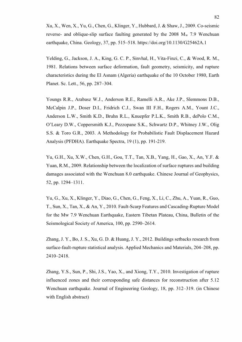
82
Xu, X., Wen, X., Yu, G., Chen, G., Klinger, Y., Hubbard, J. & Shaw, J., 2009. Co-seismic
reverse- and oblique-slip surface faulting generated by the 2008 Mw 7.9 Wenchuan
earthquake, China. Geology, 37, pp. 515–518. https://doi.org/10.1130/G25462A.1
Yelding, G., Jackson, J. A., King, G. C. P., Sinvhal, H., Vita-Finzi, C., & Wood, R. M.,
1981. Relations between surface deformation, fault geometry, seismicity, and rupture
characteristics during the El Asnam (Algeria) earthquake of the 10 October 1980, Earth
Planet. Sc. Lett., 56, pp. 287–304.
Youngs R.R., Arabasz W.J., Anderson R.E., Ramelli A.R., Ake J.P., Slemmons D.B.,
McCalpin J.P., Doser D.I., Fridrich C.J., Swan III F.H., Rogers A.M., Yount J.C.,
Anderson L.W., Smith K.D., Bruhn R.L., Knuepfer P.L.K., Smith R.B., dePolo C.M.,
O’Leary D.W., Coppersmith K.J., Pezzopane S.K., Schwartz D.P., Whitney J.W., Olig
S.S. & Toro G.R., 2003. A Methodology for Probabilistic Fault Displacement Hazard
Analysis (PFDHA). Earthquake Spectra, 19 (1), pp. 191-219.
Yu, G.H., Xu, X.W., Chen, G.H., Gou, T.T., Tan, X.B., Yang, H., Gao, X., An, Y.F. &
Yuan, R.M., 2009. Relationship between the localization of surface ruptures and building
damages associated with the Wenchuan 8.0 earthquake. Chinese Journal of Geophysics,
52, pp. 1294–1311.
Yu, G., Xu, X., Klinger, Y., Diao, G., Chen, G., Feng, X., Li, C., Zhu, A., Yuan, R., Guo,
T., Sun, X., Tan, X., & An, Y., 2010. Fault-Scarp Features and Cascading-Rupture Model
for the Mw 7.9 Wenchuan Earthquake, Eastern Tibetan Plateau, China, Bulletin of the
Seismological Society of America, 100, pp. 2590–2614.
Zhang, J. Y., Bo, J. S., Xu, G. D. & Huang, J. Y., 2012. Buildings setbacks research from
surface-fault-rupture statistical analysis. Applied Mechanics and Materials, 204–208, pp.
2410–2418.
Zhang, Y.S., Sun, P., Shi, J.S., Yao, X., and Xiong, T.Y., 2010. Investigation of rupture
influenced zones and their corresponding safe distances for reconstruction after 5.12
Wenchuan earthquake. Journal of Engineering Geology, 18, pp. 312–319. (in Chinese
with English abstract)

83
Zhang, Y.S., Shi, J.S., Sun, P., Yang, W., Yao, X., Zhang, C.S. & Xiong, T.Y., 2013.
Surface ruptures induced by the Wenchuan earthquake: their influence widths and safety
distances for construction sites, Engineering Geology, 166, pp. 245–254.
Zhou, Q., Xu, X., Yu, G., Chen, X., He, H., and Yin, G., 2010. Width Distribution of the
Surface Ruptures Associated with the Wenchuan Earthquake: implication for the Setback
Zone of the Seismogenic Faults in Post-earthquake Reconstruction, Bulletin of the
Seismological Society of America, 100, pp. 2660–2668.
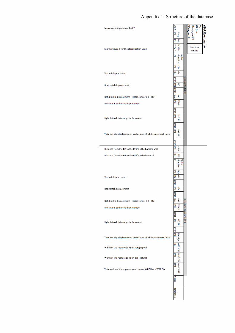
Appendix 1. Structure of the database
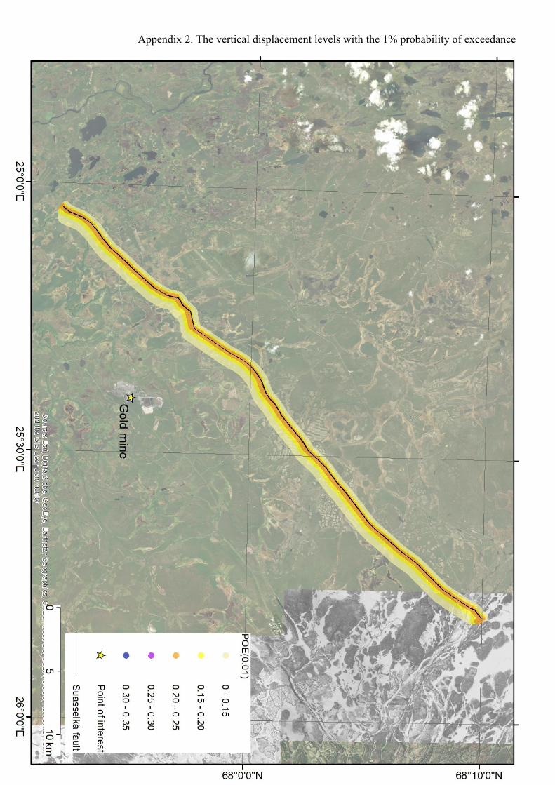
Appendix 2. The vertical displacement levels with the 1% probability of exceedance
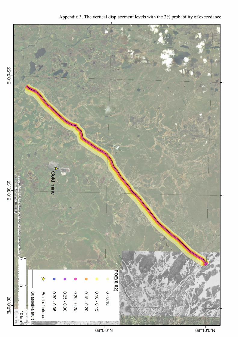
Appendix 3. The vertical displacement levels with the 2% probability of exceedance