MIT Joint Program on theScience and Policy of Global Change

Probabilistic Forecast for 21st CenturyClimate Based on Uncertainties in Emissions

(without Policy) and Climate ParametersA.P. Sokolov, P.H. Stone, C.E. Forest, R. Prinn, M.C. Sarofim, M. Webster,

S. Paltsev, C.A. Schlosser, D. Kicklighter, S. Dutkiewicz, J. Reilly, C. Wang,B. Felzer, J. Melillo, and H.D. Jacoby

Report No. 169January 2009

The MIT Joint Program on the Science and Policy of Global Change is an organization for research,independent policy analysis, and public education in global environmental change. It seeks to provide leadershipin understanding scientific, economic, and ecological aspects of this difficult issue, and combining them into policyassessments that serve the needs of ongoing national and international discussions. To this end, the Program bringstogether an interdisciplinary group from two established research centers at MIT: the Center for Global ChangeScience (CGCS) and the Center for Energy and Environmental Policy Research (CEEPR). These two centersbridge many key areas of the needed intellectual work, and additional essential areas are covered by other MITdepartments, by collaboration with the Ecosystems Center of the Marine Biology Laboratory (MBL) at Woods Hole,and by short- and long-term visitors to the Program. The Program involves sponsorship and active participation byindustry, government, and non-profit organizations.

To inform processes of policy development and implementation, climate change research needs to focus onimproving the prediction of those variables that are most relevant to economic, social, and environmental effects.In turn, the greenhouse gas and atmospheric aerosol assumptions underlying climate analysis need to be related tothe economic, technological, and political forces that drive emissions, and to the results of international agreementsand mitigation. Further, assessments of possible societal and ecosystem impacts, and analysis of mitigationstrategies, need to be based on realistic evaluation of the uncertainties of climate science.

This report is one of a series intended to communicate research results and improve public understanding of climateissues, thereby contributing to informed debate about the climate issue, the uncertainties, and the economic andsocial implications of policy alternatives. Titles in the Report Series to date are listed on the inside back cover.

Henry D. Jacoby and Ronald G. Prinn,Program Co-Directors

For more information, please contact the Joint Program OfficePostal Address: Joint Program on the Science and Policy of Global Change

400 Main StreetMIT E19-411Cambridge MA 02139-4307 (USA)

Location: 400 Main Street, CambridgeBuilding E19, Room 411Massachusetts Institute of Technology

Access: Phone: +1(617) 253-7492Fax: +1(617) 253-9845E-mail: glo balcha nge @mi t .e duWeb site: ht t p://gl o balch ange .m i t .e du / /

Printed on recycled paper

Probabilistic Forecast for 21st Century Climate Based on Uncertainties in Emissions (without Policy) and Climate Parameters

A.P. Sokolov*, P.H. Stone*, C.E. Forest*, R. Prinn*, M.C. Sarofim*, M. Webster*, S. Paltsev*, C.A. Schlosser*, D. Kicklighter†, S. Dutkiewicz*, J. Reilly*, C. Wang*, B. Felzer‡,

J. Melillo†, and H.D. Jacoby*

Abstract

The MIT Integrated Global System Model is used to make probabilistic projections of climate change from 1861 to 2100. Since the model’s first projections were published in 2003 substantial improvements have been made to the model and improved estimates of the probability distributions of uncertain input parameters have become available. The new projections are considerably warmer than the 2003 projections, e.g., the median surface warming in 2091 to 2100 is 5.1oC compared to 2.4oC in the earlier study. Many changes contribute to the stronger warming; among the more important ones are taking into account the cooling in the second half of the 20th century due to volcanic eruptions for input parameter estimation and a more sophisticated method for projecting GDP growth which eliminated many low emission scenarios. However, if recently published data, suggesting stronger 20th century ocean warming, are used to determine the input climate parameters, the median projected warning at the end of the 21st century is only 4.1oC. Nevertheless all our simulations have a very small probability of warming less than 2.4oC, the lower bound of the IPCC AR4 projected likely range for the A1FI scenario, which has forcing very similar to our median projection. The probability distribution for the surface warming produced by our analysis is more symmetric than the distribution assumed by the IPCC due to a different feedback between the climate and the carbon cycle, resulting from a different treatment of the carbon-nitrogen interaction in the terrestrial ecosystem.

Contents 1. INTRODUCTION.....................................................................................................................................................2 2. MODEL COMPONENTS.........................................................................................................................................4

2.1 Human activity and emissions ............................................................................................................................5 2.2 Atmospheric Dynamics and Physics...................................................................................................................6 2.3 Atmospheric Chemistry ......................................................................................................................................7

2.3.1 Urban Air Chemistry...................................................................................................................................7 2.3.2 Global Atmospheric Chemistry ...................................................................................................................8 2.3.3 Coupling of Global and Urban Chemistry Modules ...................................................................................9

2.4 Ocean Component...............................................................................................................................................9 2.5 Global Land System..........................................................................................................................................11

3. METHODOLOGY ..................................................................................................................................................12 3.1 General approach for making projections .........................................................................................................12 3.2 Physical/scientific uncertainties........................................................................................................................13

3.2.1 Climate sensitivity, mixing of heat into the ocean, and aerosol forcing....................................................13 3.2.2 Uncertainty in carbon cycle ......................................................................................................................15 3.2.3 Precipitation frequency .............................................................................................................................15

3.3 Economic/emissions uncertainties ....................................................................................................................17 3.4 Design of the simulations..................................................................................................................................18

4. 21st CENTURY PROJECTIONS OF ANTHROPOGENIC CLIMATE CHANGE................................................19 4.1 Greenhouse gas projections ..............................................................................................................................19 4.2 Projected changes in climate.............................................................................................................................23

* MIT Joint Program on the Science and Policy of Global Change (E-mail: Sokolov@mit.edu) † The Ecosystems Center, Marine Biological Laboratory ‡ Department of Earth and Environmental Sciences, Lehigh University

1

4.3 Changes in carbon fluxes ..................................................................................................................................28 4.4 Comparison with the IPCC AR4 projections ....................................................................................................31 4.5 Sensitivity of the projected surface warming to the deep-ocean data used to derive climate input parameters34

5. CONCLUSIONS .....................................................................................................................................................36 6. REFERENCES ........................................................................................................................................................37

1. INTRODUCTION Projections of anthropogenic global warming have from the start been confounded by the

many economic and scientific uncertainties that affect forecasts of anthropogenic emissions and the response of the climate system to these emissions (e.g., Houghton et al. 2001 and Solomon et al. 2007). Up until 2001, the uncertainties in the projected climate changes were generally dealt with by giving ranges of projected changes, but without any likelihoods being associated with these ranges. Such projections leave it to the non-expert reader to assign probabilities to the possible outcomes; Moss and Schneider (2000) advocated that projections should be given in probabilistic terms to provide more complete information.

Subsequently, considerable effort has been devoted to quantifying the scientific uncertainties associated with climate model projections for a given forcing scenario. Most notably the latest IPCC report (Meehl et al. 2007a) attempted to do this for the six SRES scenarios (Nakicenovic et al. 2000) using a variety of coupled atmosphere-ocean general circulation models (AOGCMs) and models of intermediate complexity. These projections and different sources of uncertainty have been reviewed by Knutti et al. (2008).

While formal uncertainty analysis of emissions projections was investigated a couple of decades ago (e.g. Nordhaus and Yohe 1983; Edmonds and Reilly 1985; Reilly et al. 1987) it was largely ignored by the scientific community. The IPCC SRES process eschewed formal uncertainty analysis of emissions in favor of scenario analysis (Nakicenovic et al. 2000). Despite clear statements to the contrary (Nakicenovic et al. 2000) there have been attempts in the literature to interpret the SRES scenarios in a probabilistic or quasi-probabilistic sense to investigate the joint effects of uncertainty in emissions and climate outcomes (e.g. Wigley and Raper 2001). In the latest IPCC report uncertainty ranges for possible climate changes are given separately for different SRES scenarios and reflect only uncertainty in climate system response (Meehl et al. 2007a).

The most comprehensive formal treatment of both emissions and scientific uncertainties to date is that of Webster et al. (2003). In that work, uncertainty in emissions projections was driven by uncertainty in future economic growth and technological change (Webster et al. 2002) as well as uncertainty in current levels of emissions (Olivier and Berdowski 2001). The climate system uncertainties were quantified from an analysis of observed 20th century temperature changes (Forest et al. 2002).

In this paper, we update the Webster et al. (2003) probabilistic projections of climate change from the present to 2100. The Webster et al. (2003) used the MIT Integrated Global System Model (IGSM, Prinn et al. 1999), which couples an economic component (the MIT Emissions Prediction and Policy Analysis model, EPPA (Babiker et al. 2001) to a climate model of

2

intermediate complexity (Sokolov and Stone 1998; Wang et al. 1998). The IGSM was designed to be flexible and numerically efficient and so is well-suited for use

in making probabilistic projections. For example, its climate sensitivity can be varied by changing its cloud feedback and the rate of penetration of heat into the deep ocean can be varied by changing an appropriate mixing coefficient (Sokolov et al. 2005). This flexibility allows us to avoid, to a considerable extent, the structural rigidity that limits the ability of individual coupled AOGCMs to assess uncertainty in projections of global change. Also, the use of parameters’ distributions as constrained by 20th century temperature changes allows us to cover full uncertainty ranges for the climate system properties controlled by the model parameters. The economic and emissions component of the IGSM is driven by growth in the general economy and includes representation of final consumption and trade in all goods services, including a relatively detailed treatment of factors driving emissions from energy, agriculture, waste and industrial sources as they depend on resource availabilities and technological alternatives (Paltsev et al. 2005). The IGSM was used as part of the recent US CCSP scenarios exercise to generate a set of new global scenarios of emissions with and without policy intervention (CCSP 2007) and so this work extends the scenario approach applied there to a probabilistic analysis.

Since Webster et al. (2003) was published, the IGSM has been upgraded as described by Sokolov et al. (2005). These upgrades include an increase in resolution of the atmospheric model, replacement of a zonally-averaged mixed layer ocean model by a latitude-longitude resolving one, implementation of more sophisticated land system model, and a more detailed representation of the national and regional economies of the world. In addition to the improvements made to the IGSM itself, the results presented here are based on a new analysis of factors contributing to uncertainty in emissions (Webster et al. 2008). Simulations of 20th century climate used to derive distributions of earth system properties (Forest et al. 2008) were carried out with a more complete set of natural and anthropogenic forcings than simulations used by Forest et al. (2002).

These changes led to relatively moderate changes in the distributions of both the projected emissions and the climate system’s response to a given forcing. However, due to nonlinear interactions between these factors, the net effect has been to shift the distributions of warming and sea level rise substantially upward when compared to Webster et al. (2003). As discussed in detail in later sections, the overall shift in the distribution, which doubles the previous median estimate of warming, has no single major contributing factor but rather results from the combination of several changes.

One critical factor to consider is the source of the input distributions and the sensitivity of any results to them. In particular, the distributions presented by Forest et al. (2008) were obtained using estimates of changes in deep ocean heat content for the 0-3000 m layer provided by Levitus et al. (2005). A recent update of the Levitus et al. (2005) analysis (given on the NOAA website) corrects for errors in the XBT data pointed out by Gouretski and Koltermann (2007), but nevertheless obtains virtually the same result as the original analysis. However Gouretski and Koltermann (2007) and Domingues et al. (2008), who also attempt to take into

3

account these errors, come up with different estimates of changes in the ocean heat content for the 0-3000 m layer. Sokolov et al. 2008b have shown that projections of future climate change are sensitive to the distributions of climate model parameters derived using these alternative estimates of the changes in deep-ocean heat content. For consistency with our earlier study (Webster et al. 2003) we carried out our simulations using the climate parameter distributions based on the analysis of Levitus et al. (2005). However, given the significant influence of the estimate of the ocean heat uptake on the projections, we also discuss the sensitivity of our results to other estimates of the changes in the heat content of the deep ocean.

The outline of the paper is as follows. In section 2 the updated IGSM is described. Then in section 3 we present our methodology, enumerating the uncertainties taken into account, how they are characterized, and how the probabilistic projections are made. In section 4 we give our 21st century projections for a variety of indicators of changes in the earth system including greenhouse gas (GHG) concentrations, surface air temperature (SAT) changes, and sea-level rise (SLR) and we compare our results with those of Webster et al. (2003) and the IPCC's AR4. Finally we give our conclusions in section 5.

2. MODEL COMPONENTS

The MIT Integrated Global System Model includes sub-models of the relevant parts of the natural earth system and a model of the human activity. A description of the IGSM Version 1, along with sensitivity tests of key aspects of its behavior, was reported in Prinn et al. (1999). Version 2 of the IGSM (IGSM2, Sokolov et al. 2005) includes the following components (Figure 1):

A model of human activities and emissions (the Emissions Prediction and Policy Analysis Model),

An atmospheric dynamics, physics and chemistry model, which includes a sub-model of urban chemistry,

A mixed layer/ anomaly diffusing ocean model (ADOM) with carbon cycle and sea ice sub-models,

A land system model that combines the Terrestrial Ecosystem Model (TEM), a Natural Emissions Model (NEM), and the Community Land Model (CLM), that together describe the global, terrestrial water and energy budgets and terrestrial ecosystem processes.

The Earth climate system component of the IGSM is a fully coupled model which allows simulation of critical feedbacks between components. The time steps used in the various sub-models range from 10 minutes for atmospheric dynamics to 1 month for TEM, reflecting differences in the characteristic timescales of the various processes simulated by the IGSM.

The IGSM is distinguished from other similar models by its inclusion of significant chemical and biological detail. Our models of the terrestrial carbon, methane and nitrous oxide cycles are coupled to climate, terrestrial hydrology and land ecosystems models, which provide the needed explicit predictions of temperature, rainfall, and soil organic carbon concentrations. The prediction of global anthropogenic emissions of CO2, CO, NOx, black carbon, SOx and other key

4

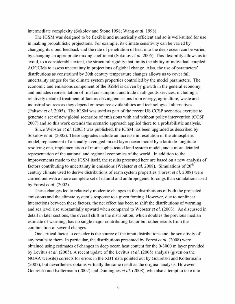
species is based on a regionally disaggregated model of global economic growth. This procedure allows for treatment over time of a shifting geographical distribution of emissions, changing mixes of these emissions, and recognition of the fact that the emissions of chemicals important in air pollution and climate are highly correlated due to shared generating processes like combustion.

Figure 1. The MIT IGSM version 2.2

The major model components of the IGSM2 and recent developments in their capabilities and linkages are summarized below.

2.1 Human activity and emissions

The Emissions Prediction and Policy Analysis (EPPA) Model is a general equilibrium model of the world economy developed by the MIT Joint Program on the Science and Policy of Global Change (Paltsev et al. 2005). For economic data, it relies on the GTAP dataset (Dimaranan and McDougall, 2002), which accommodates a consistent representation of regional macroeconomic consumption, production and bilateral trade flows. The energy data in physical units are based on energy balances from the International Energy Agency. EPPA model also uses additional data for past greenhouse gas emissions (carbon dioxide, CO2; methane, CH4; nitrous oxide, N2O; hydrofluorocarbons, HFCs; perfluorocarbons, PFCs; and sulphur hexafluoride, SF6) and past air pollutant emissions (sulphur dioxide, SO2; nitrogen oxides, NOx; black carbon, BC; organic

5

carbon, OC; ammonia, NH3; carbon monoxide, CO; and non-methane volatile organic compounds, VOC) based on United States Environmental Protection Agency inventory data supplemented by our own estimates.

Much of the model’s sectoral detail is focused on energy production to represent technological alternatives in electric generation and transportation. From 2000 to 2100 the model is solved recursively at 5-year intervals. The EPPA model production and consumption sectors are represented by nested Constant Elasticity of Substitution (CES) production functions (or the Cobb-Douglas and Leontief special cases of the CES). The model is written in the GAMS software system and solved using MPSGE modeling language (Rutherford 1995). The EPPA model has been used in a wide variety of policy applications (e.g., Jacoby et al. 1997; Reilly et al. 1999; Babiker et al. 2003; Reilly and Paltsev 2006; US CCSP 2007; Paltsev et al. 2008).

Because climate and energy policy are our main focus, the model further disaggregates the data for transportation and existing energy supply technologies and as well includes a number of alternative sources that are not in widespread use now, but could take market share in the future under changed energy prices or climate policy conditions. Bottom-up engineering details are incorporated in EPPA model in the representation of these alternative energy supply technologies. The competitiveness of different technologies depends on the endogenously determined prices for all inputs, and those prices depend in turn on depletion of resources, economic policy, and other forces driving economic growth such as savings, investment, energy-efficiency improvements, and productivity of labor. Additional information on the model’s structure can be found in Paltsev et al. (2005).

2.2 Atmospheric Dynamics and Physics

The MIT two-dimensional (2D) atmospheric dynamics and physics model (Sokolov and Stone 1998) is a zonally averaged statistical-dynamical model that explicitly solves the primitive equations for the zonal mean state of the atmosphere and includes parameterizations of heat, moisture, and momentum transports by large scale eddies based on baroclinic wave theory (Stone and Yao 1987 and 1990). The model’s numerics and parameterizations of physical processes, including clouds, convection, precipitation, radiation, boundary layer processes, and surface fluxes, are built upon those of the Goddard Institute for Space Studies (GISS) GCM (Hansen et al. 1983). The radiation code includes all significant greenhouse gases (H2O, CO2, CH4, N2O, CFCs and O3) and eleven types of aerosols. The model’s horizontal and vertical resolutions are variable, but the standard version of IGSM2 has 4° resolution in latitude and eleven levels in the vertical.

The MIT 2D atmospheric model allows up to four different types of underlying surface in each grid cell (ice free ocean, sea-ice, land, and land-ice). The surface characteristics (e.g., temperature, soil moisture, albedo) as well as turbulent and radiative fluxes are calculated separately for surface type. The atmosphere above is assumed to be well mixed zonally in each latitudinal band. The area-weighted fluxes from the different surface types are used to calculate the change of temperature, humidity, and wind speed in the atmosphere. Convection and large-

6

scale condensation are simulated under the assumptions that a zonal band may be partially unstable or partially saturated, respectively. The moist convection parameterization, which was originally designed for the GISS Model I (Hansen et al. 1983), requires knowledge of sub-grid scale temperature variance. Zonal temperature variance associated with transient eddies is calculated using a parameterization proposed by Branscome (see Yao and Stone 1987). The variance associated with stationary eddies was represented in the IGSM1 by adding a fixed variance of 2 K at all latitudes. In the IGSM2 we introduce a latitudinal dependence of the latter variance that follows more closely the climatological pattern (see Figure. 7.8b of Peixoto and Oort 1992). In addition, the threshold values of relative humidity for the formation of large-scale cloud and precipitation have been modified such that a constant value for all latitudes (as used in the IGSM1) is replaced with latitudinally varying values. This modification is made to account for the dependence of the zonal variability of relative humidity on latitude. Zonal precipitations simulated by atmospheric model are partitioned into land and ocean components using present day climatology. These changes led to an improvement in the zonal pattern of the annual cycle of land precipitation and evapotranspiraton (Schlosser at al. 2007).

The atmospheric model’s climate sensitivity can be changed by varying the cloud feedback. The method for changing this feedback in the model has been changed from the method used previously. In the IGSM1 the cloud cover at all levels was changed by a fixed fraction, which depended on the global mean surface temperature (Sokolov and Stone 1998). In the IGSM2 high cloud covers and low cloud covers are changed in opposite directions by a constant factor, which is again dependent on the global mean surface temperature. The new method, described by Sokolov (2006), shows better agreement with changes simulated by AOGCMs.

2.3 Atmospheric Chemistry

To calculate atmospheric composition, the model of atmospheric chemistry includes an analysis of the climate-relevant reactive gases and aerosols at urban scales, coupled to a model of the processing of exported pollutants from urban areas (plus the emissions from non-urban areas) at the regional to global scale. For calculation of the atmospheric composition in non-urban areas, the above atmospheric dynamics and physics model is linked to a detailed 2D zonal mean model of atmospheric chemistry. The atmospheric chemical reactions are thus simulated in two separate modules, one for the 2D model grids and one for the sub-grid-scale urban chemistry.

2.3.1 Urban Air Chemistry

The analysis of the atmospheric chemistry of key substances as they are emitted into polluted urban areas is an important addition to the integrated system since the version described in Prinn et al. (1999). Urban air pollution is explicitly treated in the IGSM for several reasons. It has a significant impact on global methane, ozone and aerosol chemistry, and thus on climate. However, the nonlinearities in the chemistry cause urban emissions to undergo different net transformations than rural emissions. Accuracy in describing these transformations is necessary because the atmospheric lifecycles of exported air pollutants such as CO, O3, NOx and VOCs, and the climatically important species CH4 and sulfate aerosols, are linked through the fast

7

photochemistry of the hydroxyl free radical (OH) as we will emphasize in the results discussed later in section 5. Urban air-shed conditions need to be resolved at varying levels of pollution. The urban air chemistry model must also provide detailed information about particulates and their precursors important to air chemistry and human health, and about the effects of local topography and structure of urban development on the level of containment and thus the intensity of air pollution events. This is an important consideration because air pollutant levels are dependent on projected emissions per unit area, not just total urban emissions.

The urban atmospheric chemistry model has been introduced as an additional component to the original global model (Prinn et al. 1999) in IGSM1 (Calbo et al. 1998; Mayer et al. 2000; Prinn et al. 2007). It was derived by fitting multiple runs of the detailed 3D California Institute of Technology (CIT) Urban Airshed Model, adopting the probabilistic collocation method to express outputs from the CIT model in terms of model inputs using polynomial chaos expansions (Tatang et al. 1997). This procedure results in a reduced format model to represent about 200 gaseous and aqueous pollutants and associated reactions over urban areas that is computationally efficient enough to be embedded in the global model. The urban module is formulated to take meteorological parameters including wind speed, temperature, cloud cover, and precipitation as well as urban emissions as inputs. Calculated with a daily time step, it exports fluxes along with concentrations (peak and mean) of selected pollutants to the global model.

2.3.2 Global Atmospheric Chemistry

The 2D zonal mean model that is used to calculate atmospheric composition is a finite difference model in latitude-pressure coordinates, and the continuity equations for trace constituents are solved in mass conservative or flux form (Wang et al. 1998). The model includes 33 chemical species. The continuity equations for CFCl3, CF2Cl2, N2O, O3, CO, CO2, NO, NO2, N2O5, HNO3, CH4, CH2O, SO2, H2SO4, HFC, PFC, SF6, black carbon aerosol, and organic carbon aerosol include convergences due to transport, parameterized north-south eddy transport, convective transports, local true production or loss due to surface emission or deposition, and atmospheric chemical reactions. In contrast to these gases and aerosols, the very reactive atoms (e.g., O), free radicals (e.g., OH), or molecules (e.g., H2O2) are assumed to be unaffected by transport because of their very short lifetimes; only chemical production and/or loss (in the gaseous or aqueous phase) is considered in the predictions of their atmospheric abundances.

There are 41 gas-phase and twelve heterogeneous reactions in the background chemistry module applied to the 2D model grid. The scavenging of carbonaceous and sulfate aerosol species by precipitation is also included using a method based on a detailed 3D climate-aerosol-chemistry model (Wang 2004). Water vapor and air (N2 and O2) mass densities are computed using full continuity equations as a part of the atmospheric dynamics and physics model to which the chemical model is coupled. The climate model also provides wind speeds, temperatures, solar radiation fluxes and precipitation, which are used in both the global and urban chemistry formulations.

8

2.3.3 Coupling of Global and Urban Chemistry Modules

The urban chemistry module was derived based on an ensemble of 24-hour long CIT model runs and thus is processed in the IGSM with a daily time step, while the global chemistry module is run in a real time step with the dynamics and physics model, 20 minutes for advection and scavenging, 3 hours for tropospheric reactions. The two modules in the IGSM are processed separately at the beginning of each model day, supplied by emissions of non-urban and urban regions, respectively. At the end of each model day, the predicted concentrations of chemical species by the urban and global chemistry modules are then remapped based on the urban to non-urban volume ratio at each model grid. Beyond this step, the resultant concentrations at each model grid will be used as the background concentration for the next urban module prediction and also as initial values for the global chemistry module (Mayer et al. 2000).

2.4 Ocean Component

In the older IGSM1 (Prinn et al. 1999) a zonally averaged mixed layer ocean model with 7.8° latitudinal resolution was used. In the new IGSM2 the ocean component has been replaced by either a two-dimensional (latitude-longitude) mixed layer anomaly-diffusing ocean model (hereafter denoted as IGSM2.2) or a fully three-dimensional ocean GCM (denoted as IGSM2.3). Dalan et al. (2005b) showed that different versions of the 3-D ocean model with different rates of heat uptake can be produced by changing the vertical/diapycnal diffusion coefficients. However, changing the diapycnal coefficient also alters the ocean circulation, in particular the strength of North Atlantic overturning (Dalan et al. 2005a). Unfortunately it appears infeasible (certainly without changes to parameterizations in the 3-D models) to vary the heat uptake over the full range consistent with observations during the 20th century (Forest et al. 2008) and at the same time to maintain a reasonable circulation.

The ocean component of the IGSM2.2 consists of a Q-flux mixed layer model with horizontal resolution of 4° in latitude and 5° in longitude, and a 3000m deep anomaly diffusing ocean model beneath. The mixed layer depth is prescribed based on observations as a function of time and location (Hansen et al. 1983). In addition to the temperature of the mixed layer, the model also calculates the averaged temperature of the seasonal thermocline and the temperature at the annual maximum mixed layer depth (Russell et al. 1985). Diffusion in the deep ocean model is applied to the difference in the temperature at the bottom of the seasonal thermocline relative to its value in a present-day climate simulation (Hansen et al. 1984; Sokolov and Stone 1998). Since this diffusion represents a cumulative effect of heat mixing by all physical processes, the values of the diffusion coefficients are significantly larger than those used in sub-grid scale diffusion parameterizations in OGCMs. The spatial distribution of the diffusion coefficients used in the diffusive model is based on observations of tritium mixing into the deep ocean (Hansen et al. 1988). For simulations with different rates of oceanic heat uptake, the coefficients are scaled by the same factor in all locations.

The coupling between the atmospheric and oceanic components takes place every hour and is described by Kamenkovich et al. (2002) and Sokolov et al. (2005).

9

The mixed layer model also includes a specified vertically-integrated horizontal heat transport by the deep oceans, a so-called “Q-flux”, allowing zonal as well as meridional transport. This flux is calculated from a simulation in which sea surface temperature (SST) and sea ice distribution are relaxed toward their present-day climatology with relaxation coefficient of 300 W/m2/K, which corresponds to an e-folding time scale of about 15 days for a 100 m deep mixed layer. Relaxing SST and sea ice on such a short time scale, while being virtually identical to specifying them, avoids problems with calculating the Q-flux near the sea ice edge. The use of a two-dimensional (longitude-latitude) mixed layer ocean model instead of the zonally averaged one used in IGSM1 has allowed a better simulation of both the present day sea ice distribution and sea ice changes in response to increasing radiative forcing (Sokolov et al. 2005).

A thermodynamic ice model is used for representing sea ice. This model has two ice layers and computes ice concentration (the percentage of area covered by ice) and ice thickness.

The IGSM2.2 includes a significantly modified version of the ocean carbon model (Holian et al. 2001) used in the IGSM1. Formulation of carbonate chemistry (Follows et al. 2006) and parameterization of air-sea fluxes in this model are similar to the ones used in the IGSM2.3. Vertical and horizontal transports of the total dissolved inorganic carbon, though, are still parameterized by diffusive processes. The values of the horizontal diffusion coefficients are taken from Stocker et al. (1994), and the coefficient of vertical diffusion of carbon (Kvc) depends on the coefficient of vertical diffusion of heat anomalies (Kv). In IGSM1, Kvc was assumed to be proportional to Kv (Prinn et al. 1999; Sokolov et al. 1998). This assumption, however, does not take into account the vertical transport of carbon due to the biological pump. In the IGSM2.2 Kvc is, therefore, defined as:

Kvc = Kvco + rKv (1) Since Kvco is a constant, the vertical diffusion coefficients for carbon have the same

latitudinal distribution as the coefficients for heat. For simulations with different rates of oceanic uptake, the diffusion coefficients are scaled by the same factor in all locations. Therefore rates of both heat and carbon uptake by the ocean are defined by the global mean value of the diffusion coefficient for heat. In the rest of the paper the symbol Kv is used to designate the global mean value.

Comparisons with 3D ocean simulations have shown that the assumption that changes in ocean carbon can be simulated by the diffusive model with fixed diffusion coefficient, as used in the IGSM1, works only for about 150 years. On longer timescales the simplified carbon model overestimates the ocean carbon uptake. However, if Kvc is assumed to be time dependent, the IGSM2.2 reproduces changes in ocean carbon as simulated by the IGSM2.3 on multi century scales (Sokolov et al. 2007). Thus, for the runs discussed here, the coefficient for vertical diffusion of carbon was calculated as:

Kvc(t) = (Kvco + rKv) . f(t) (2) Where f(t) is a time dependent function constructed based on the analyses of the depths of

carbon mixing in simulations with the IGSM2.3.

10

To evaluate the performance of the anomaly diffusing ocean model (ADOM) on different time scales Sokolov et al. (2007) carried out a detailed comparison of the results of simulations with the two versions of the IGSM2. Our results show that in spite of its inability to depict feedbacks associated with the changes in the ocean circulation and a very simple parameterization of the ocean carbon cycle, the version of the IGSM2 with the ADOM is able to reproduce the important aspects of the climate response simulated by the version with the OCGM through the 20th and 21st century and can be used to obtain probability distributions of changes in many of the important climate variables, such as surface air temperature and sea level, through the end of 21st century.

2.5 Global Land System

The Global Land System framework (GLS, Schlosser et al. 2007) integrates three existing models: the Community Land Model (CLM, e.g. Bonan et al. 2002), the Terrestrial Ecosystems Model (TEM, e.g. Melillo et al. 1993), and a Natural Emissions Model (NEM, Liu 1996). The GLS uses the CLM representation of the coupling of the biogeophysical characteristics and fluxes between the atmosphere and land (e.g., evapotranspiration, surface temperatures, albedo, surface roughness, and snow depth). In addition, the CLM provides all of the hydrothermal states and fluxes (e.g., soil moisture, soil temperatures, evaporation, and precipitation events) at the appropriate spatial and temporal scales required by TEM and NEM. The TEM is then used to estimate changes in terrestrial carbon storage and the net flux of carbon dioxide between land and the atmosphere as a result of ecosystem metabolism. The NEM estimates the net flux of methane from global wetlands and tundra ecosystems and the net flux of nitrous oxide from all natural terrestrial ecosystems to the atmosphere. The sub-module in NEM describing processes leading to nitrous oxide emissions is primarily a globalization of the Denitrification Decomposition (DNDC) model of Li et al. (1992). Within the GLS, the algorithms of NEM that describe methane (CH4) and nitrous oxide (N2O) dynamics have been incorporated into TEM so that TEM now describes the hourly and daily dynamics of these trace gases in addition to the monthly dynamics of carbon dioxide and organic matter in terrestrial ecosystems. The direct coupling between these two models allows monthly TEM estimates of reactive soil organic carbon to determine nitrous oxide fluxes. In addition, a new procedure has been developed that provides a statistical representation of the episodic nature and spatial distribution of land precipitation. This is required for two reasons: 1) an “episodic” provision of zonal precipitation from the IGSM’s atmospheric sub-model represents more realistic hydrologic forcing to CLM than a constant precipitation rate applied at every time step for every zonal band, and 2) the N2O module of NEM requires precipitation events that vary in intensity and duration along with corresponding dry periods between storm events to employ its decomposition, nitrification, and denitrification parameterizations.

All land areas across the globe are assumed by TEM and NEM to be covered by natural vegetation, which is held constant in time. To match and couple with the zonal configuration of the atmospheric dynamics and chemistry, the areas for each land cover type at the native 0.5o

11

latitude x 0.5o longitude grid cells (employed by both CLM and TEM) have been aggregated within each 4o latitudinal band used by the atmospheric dynamics and chemistry model (Schlosser et al. 2007). Thus, each latitudinal band represents a 4o latitude x 360o longitude grid cell in the GLS framework. The GLS is run for all land cover types found in these zonal cells and the area covered by each land cover type is used to determine the relative contribution of that land cover type to the zonally aggregated water, energy, carbon and nitrogen fluxes from the terrestrial systems. As shown by Schlosser et al. (2007), the zonal fluxes from GLS are not substantially affected by the implementation the of zonal mosaic land cover data in the IGSM2 as compared to their performance using explicit latitude/longitude grids. The timing and location of the carbon sink sand source regions is preserved, and the spatiotemporal patterns of evapotranspiration agree well with a consensus of state-of-the-art biogeophysical models as determined by the Global Soil Wetness Project Phase 2 (GSWP2, Dirmeyer et al. 2002). Moreover, one of the more desirable changes in the patterns of carbon flux by TEM in the zonal GLS configuration, as compared to a previous version of TEM employed in the IGSM, is the removal of an erroneous, mid-summer carbon emission at northern high latitudes, which is not seen in spatially explicit TEM simulations forced by observed atmospheric conditions (refer to Schlosser et al. 2007, for more details).

In TEM, the potential uptake of atmospheric CO2 by plants is assumed to follow Michaelis-Menten kinetics, according to which the effect of atmospheric CO2 at time t on the assimilation of CO2 by plants is parameterized as follows:

f(CO2(t)) = (Cmax CO2(t)) / (kc + CO2(t) ) (3) where Cmax is the maximum rate of C assimilation, and kc is the CO2 concentration at which C assimilation proceeds at one-half of its maximum rate (i.e. Cmax). The sensitivity of plant uptake on kc is defined not by the absolute value of f(CO2(t)), which decreases with kc, but by the ratio of f(CO2(t)) to f(CO2(0)) which increases with kc. This ratio can be approximated as 1+αlog(CO2(t)/ CO2(0)). In contrast to most of the terrestrial biosphere models currently used in climate change assessments (Plattner et al. 2008), TEM takes in to account nitrogen limitations on net carbon storage. This significantly decrease sensitivity of the terrestrial carbon uptake to the increase in the atmospheric CO2 concentration and affect sign of the feedback between terrestrial carbon cycle and climate (Sokolov et al. 2008a).

3. METHODOLOGY

3.1 General approach for making projections

The basic method we employ for uncertainty analysis is Monte Carlo simulation, in which multiple input sets are sampled from probability distributions representing uncertainty in input parameters. Pure random sampling typically requires many thousands of samples to converge to a stable distribution of the model output. Therefore, a number of alternative more efficient sampling strategies have been developed. In this study, we use Latin Hypercube Sampling (LHS) (Iman and Helton 1988). LHS divides each parameter distribution into n segments of equal probability, where n is the number of samples to be generated. Sampling without

12

replacement is performed so that with n samples every segment is used once. We use a sample size of 400 for each s simulation ensemble.

3.2 Physical/scientific uncertainties

3.2.1 Climate sensitivity, mixing of heat into the ocean, and aerosol forcing

Three properties that are commonly recognized as being major contributors to the uncertainty in simulations of future climate change are the effective climate sensitivity of the system (S), the rate at which heat is mixed into the deep ocean (Kv), and the strength of the aerosol forcing associated with a given aerosol loading (Faer) (Meehl et al. 2007a). These same properties and their uncertainties also affect 20th century simulations. Thus in principle estimates of these properties and their uncertainties can be derived from simulations in which these properties are varied to determine which give simulations consistent with observed 20th century changes.

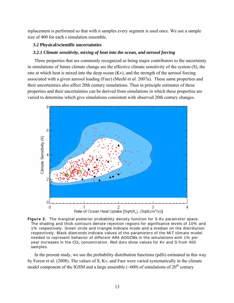
Figure 2. The marginal posterior probability density function for S-Kv parameter space.

The shading and thick contours denote rejection regions for significance levels of 10% and 1% respectively. Green circle and triangle indicate mode and a median on the distribution respectively. Black diamonds indicate values of the parameters of the MIT climate model needed to represent behavior of different AR4 AOGCMs in the simulations with 1% per year increases in the CO2 concentration. Red dots show values for Kv and S from 400 samples.

In the present study, we use the probability distribution functions (pdfs) estimated in this way by Forest et al. (2008). The values of S, Kv, and Faer were varied systematically in the climate model component of the IGSM and a large ensemble (~600) of simulations of 20th century

13

climate was carried out. The simulations were compared against observations of surface, upper-air, and deep-ocean temperature changes. For each diagnostic the likelihood that a given simulation is consistent with the observed changes, allowing for observational error and natural variability, was estimated using goodness of fit statistics from climate change detection methods (see Forest et al. 2002, 2006, 2008). By combining the likelihood distributions estimated from each diagnostic using Bayes’ Theorem, a posterior probability distribution was obtained. As with other estimates of probability distributions using Bayesian methods, priors on the three parameters are required. For climate sensitivity, the prior distribution was calculated by Webster and Sokolov (2000) from an expert elicitation by Morgan and Keith (1995). This prior essentially limits the possible climate sensitivities to being less than 7 oC, consistent with expert opinion (Webster and Sokolov 2000; Hegerl et al. 2007). Uniform distributions were used as priors for the other two parameters.

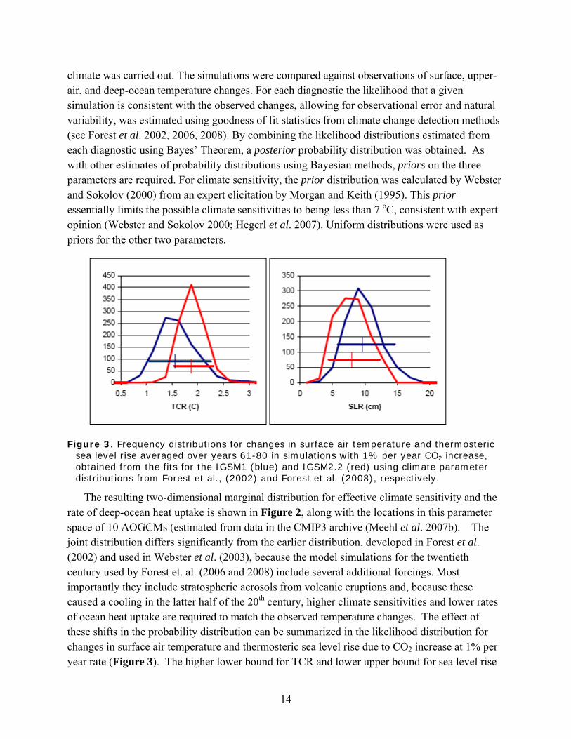
Figure 3. Frequency distributions for changes in surface air temperature and thermosteric

sea level rise averaged over years 61-80 in simulations with 1% per year CO2 increase, obtained from the fits for the IGSM1 (blue) and IGSM2.2 (red) using climate parameter distributions from Forest et al., (2002) and Forest et al. (2008), respectively.

The resulting two-dimensional marginal distribution for effective climate sensitivity and the rate of deep-ocean heat uptake is shown in Figure 2, along with the locations in this parameter space of 10 AOGCMs (estimated from data in the CMIP3 archive (Meehl et al. 2007b). The joint distribution differs significantly from the earlier distribution, developed in Forest et al. (2002) and used in Webster et al. (2003), because the model simulations for the twentieth century used by Forest et. al. (2006 and 2008) include several additional forcings. Most importantly they include stratospheric aerosols from volcanic eruptions and, because these caused a cooling in the latter half of the 20th century, higher climate sensitivities and lower rates of ocean heat uptake are required to match the observed temperature changes. The effect of these shifts in the probability distribution can be summarized in the likelihood distribution for changes in surface air temperature and thermosteric sea level rise due to CO2 increase at 1% per year rate (Figure 3). The higher lower bound for TCR and lower upper bound for sea level rise

14

are a direct result of the shift in the distributions for climate sensitivity (S) and the effective thermal diffusivity (Kv).

The LHS sampling method used in Webster et al. (2003) generated samples for Kv, S and Faer from their individual 1D marginal pdfs, and imposed the correlation structure of the joint 3D pdf on the samples. In contrast, now after picking a Kv sample from the 1D marginal pdf, we generate a 2D pdf for S and Faer conditional on the chosen Kv value, and then calculate a 1D marginal pdf for S from that 2D pdf, and sample the new pdf for S. Finally, we generate a 1D pdf for Faer conditional on the two chosen values of Kv and S , and sample that pdf for a value of Faer. This new sampling strategy preserves the uniqueness of the samples by not allowing one to choose from the same bin number in the conditional pdfs, though it theoretically may sample the same value of S or Faer few times in contrast to the earlier method. New method better preserves the full details of the original three dimensional pdf. Values for Kv and S from the 400 samples are shown on Figure 2 by red dots.

3.2.2 Uncertainty in carbon cycle

As described in section 2.4, the vertical diffusion coefficient for carbon depends on the effective vertical diffusivity for temperature anomalies, Thereby uncertainty in carbon uptake by the ocean is linked to the uncertainty in heat uptake. Values of the parameters in the equation for Kvc (Eq. 1) were estimated so that, for the range of Kv, deduced from observations, the oceanic carbon uptake for the 1980s spans the observed uncertainty range given in the IPCC TAR. The values of Kvco and r that satisfy this requirement are 1.0 cm2 s-1 and 3.0 respectively.

In contrast to Webster et al. (2003), in the present study, we take into account uncertainty in the fertilization effect of atmospheric CO2. The results of CO2-enrichment studies suggest that plant growth could increase from 24% to 50% in response to doubled CO2 given adequate nutrients and water (Raich et al. 1991; McGuire et al. 1992; Gunderson and Wullschleger 1994; Curtis and Wang 1998; Norby et al. 2005). In TEM, a value of 400 ppmv CO2 is normally chosen for the half-saturation constant kc (Eq. 3) so that f(CO2(t)) increases by 37% for a doubling of atmospheric CO2 from 340 ppmv to 680 ppmv CO2 (McGuire et al. 1992, 1993, 1997; Pan et al. 1998). A 24% response to doubled CO2 would correspond to a kc value of 215 ppmv CO2 whereas a 50% ppmv CO2 response would correspond to a kc value of 680 ppmv CO2, for the same changes in atmospheric CO2. As these enrichment studies may not have covered the full range of uncertainty, we used 150 ppmv as a low bound for kc and 700 ppmv as the upper limit.

3.2.3 Precipitation frequency

Another physical uncertainty in the coupled earth system model is how the frequency of precipitation changes with increases in surface temperature. Changes in mean precipitation (over space and time) are fundamentally a result of shifts in the character of individual precipitation events, which are determined by the frequency at which they occur as well as their (expected) duration and intensity. It is these quantities that, in large part, determine the hydrologic climate of any region (i.e. the partitioning of precipitation between evaporation and runoff) as well as the

15

ecology and biogeochemistry of the ecosystems. For example, more runoff results in greater flood potential, less water infiltration into the soils and less storage available to plants, as well as fewer saturating events that can impede nitrous oxide emissions (from soils) as well as methane-emitting environments. Such responses to climate change can have substantial consequences on natural and managed terrestrial systems, as well as providing potentially strong feedback mechanisms to the rest of the climate system. We therefore introduce an approach that provides a probability-based extrapolation of precipitation frequency change associated with climate warming.

Lacking observations adequate for estimating this trend, we use the results of the AOGCMs that participated in the IPCC AR4 to develop probability distributions of the trend. From the model archive, we consider the pre-industrial control runs and the transient CO2 doubling runs, in which the daily outputs of precipitation are archived for at least a 20-year period. For every grid point of the GCMs’ time series, we determine for each day whether or not the model produced a sufficient amount of precipitation to be construed as a “wet” day. In doing so, our calculations require a threshold value for the daily precipitation rate of a grid cell above which we deem a precipitation “event” has occurred for that day. For this threshold we have chosen 2.5 mm/day (see Schlosser and Webster, 2008 for details). From this, we determine for each month of the simulation period the total number of days that a precipitation event occurred, and subsequently the average number of days between “wet” days for the month. To obtain a representative monthly climatology of these precipitation intervals, we calculate these statistics for each month, for every grid cell, and average them over the 20-year period for the pre-industrial runs as well as the transient run, the latter centered at the time of doubling of CO2. Then, by taking the difference in these monthly constructions of precipitation interval, we can make an inference as to any particular GCM’s propensity to change under forced climate change (i.e. to a doubling of CO2 concentrations). Then, to configure these results to the IGSM zonal atmospheric structure, these gridded results are averaged over each of the GCMs’ latitude bands, and then pooled into latitudinal regions with common statistical traits (i.e. sign, magnitude, etc.) that correlate well with the large-scale circulations and precipitation patterns. Once obtained, these (simulated) changes in this derived hydrologic diagnostic are associated with each AOGCM’s change in global temperature. Thus, the zonally-averaged changes in precipitation interval from each AOGCM are normalized according to their global temperature change.

Once we have calculated these pooled, zonally-averaged normalized changes in precipitation interval, based on the AR4 AOGCMs, we fit probability density functions to the distributions from the models. Each zonal band has a probability distribution of temperature-dependent trends, but additionally we impose correlation across zonal groups to reflect the observed correlations in the AOGCM results. As with other uncertain parameters, we perform Latin Hypercube sampling from these distributions, while imposing the observed zonal correlation structure within samples.

16

3.3 Economic/emissions uncertainties

The uncertainty in the emissions of all greenhouse gases and pollutants are taken from an uncertainty analysis of the Emissions Projection and Policy Analysis model (Paltsev et al. 2005). This analysis is summarized briefly here; see Webster et al (2008) for more detail. Compared with previous efforts (Webster et al. 2002 and 2003) several aspects of the EPPA model and of the uncertainty analysis have been improved. The technological detail of the model has been deepened, with the explicit representation of private automobiles, commercial transportation, and the service sector and the addition of biofuels as a low carbon alternative in transportation.

The characterization of emissions coefficients for pollutants was substantially changed. Whereas in previous versions of EPPA we relied on a Kuznets curve approach, the specification now used in the Monte Carlo analysis estimates an advancing technological frontier and catch-up to this frontier by lagging regions. Statistical work by Stern (2006 and 2005) has suggested this approach better represents the process. Also, the specification of uncertainty in economic growth has been substantially revised. Rather than sampling high or low growth rates that applied to the 100 year horizon as has been done previously in most Monte Carlo studies of emissions, we created stochastic growth paths characterized as a random walk where the uncertainty was estimated for each region/country for the period 1950-2000. As a result, regions experience periods of boom and bust over the 100 year horizon like that which characterized growth in the latter half of the last century rather than smooth growth that was either fast or slow.

These new approaches for representing uncertainty in productivity growth and in emissions coefficients allowed us to draw more directly from historical data to estimate uncertainty distributions rather than to rely on expert judgment, and to simulate growth patterns that varied across regions and over time that are more realistic. The new approach to simulating uncertainty in growth of gross domestic product (GDP) has narrowed the distribution of outcomes because regional growth rates are uncorrelated with each other. The result is that range of possible growth for individual regions is wide, but the global range is narrower as statistically rapid growth in some regions is likely to be offset by slow growth in other regions. The new approach on emissions coefficients for other pollutants results in lower median emissions of pollutants like SOx, NOx, and CO.

Uncertainty in emissions were developed from the EPPA model using the same Latin Hypercube Sampling approach employed here, creating a 400 member ensemble to match to match the 400 sample sets for the earth system model components (Webster et al.2008). Each of these 400 EPPA simulations provides a set of emissions for all pollutant species that are consistent: to the extent that emissions of different species derive from the same combustion sources (e.g., oil, gas, coal) they are each consistent with the amount of fuel combusted given uncertainty in emissions per unit of fuel. Each emission set is then considered to be one emissions sample that is paired randomly with one set of values for the climate parameters following the LHS protocol of sampling without replacement.

17

3.4 Design of the simulations

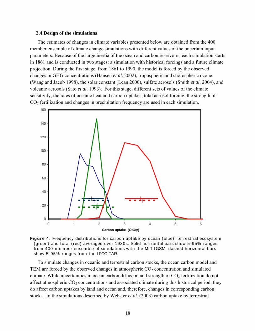
The estimates of changes in climate variables presented below are obtained from the 400 member ensemble of climate change simulations with different values of the uncertain input parameters. Because of the large inertia of the ocean and carbon reservoirs, each simulation starts in 1861 and is conducted in two stages: a simulation with historical forcings and a future climate projection. During the first stage, from 1861 to 1990, the model is forced by the observed changes in GHG concentrations (Hansen et al. 2002), tropospheric and stratospheric ozone (Wang and Jacob 1998), the solar constant (Lean 2000), sulfate aerosols (Smith et al. 2004), and volcanic aerosols (Sato et al. 1993). For this stage, different sets of values of the climate sensitivity, the rates of oceanic heat and carbon uptakes, total aerosol forcing, the strength of CO2 fertilization and changes in precipitation frequency are used in each simulation.

Figure 4. Frequency distributions for carbon uptake by ocean (blue), terrestrial ecosystem

(green) and total (red) averaged over 1980s. Solid horizontal bars show 5-95% ranges from 400-member ensemble of simulations with the MIT IGSM, dashed horizontal bars show 5-95% ranges from the IPCC TAR.

To simulate changes in oceanic and terrestrial carbon stocks, the ocean carbon model and TEM are forced by the observed changes in atmospheric CO2 concentration and simulated climate. While uncertainties in ocean carbon diffusion and strength of CO2 fertilization do not affect atmospheric CO2 concentrations and associated climate during this historical period, they do affect carbon uptakes by land and ocean and, therefore, changes in corresponding carbon stocks. In the simulations described by Webster et al. (2003) carbon uptake by terrestrial

18

ecosystem was adjusted to balance carbon cycle for the 1980s. No such adjustment is used in the present study. The resulting frequency distributions for the terrestrial, oceanic and total carbon uptake are shown Figure 4. Our ranges of carbon uptake by the ocean and the terrestrial ecosystem are somewhat narrower than those given in the IPCC TAR. However the distribution for the total uptake is rather wide with a 90% range from 2.1 to 4.0 GtC/year.

In the second-stage of the simulations, which begins in 1991, the full version of IGSM2 is forced by emissions of greenhouse gases and aerosol precursors. Historical emissions are used through 1996 and emissions projected by the EPPA model from 1997 to 2100. In this future climate stage of the simulations, concentrations of all gases and aerosols are calculated by the atmospheric chemistry sub-model based on anthropogenic and natural emissions and the terrestrial and oceanic carbon uptake provided by the corresponding sub-components. In these simulations changes in concentration of black carbon aerosol are explicitly calculated. Since they were not considered in the preceding stage, the total aerosol forcing assumed in the first stage was adjusted to take the black carbon contribution into account. Uncertainties in the economic factors that affect anthropogenic emissions are taken into account in addition to climate related uncertainties.

To evaluate the contributions to the total uncertainty in the projected climate changes due to the separate uncertainties in emissions and climate characteristics, we carried out two additional 400 member ensembles of simulations that each includes the uncertainties from just one of these two sources. In the first set of simulations the median values of the climate parameters were used while the uncertainty in the emissions was included, and in the second the median values of the emissions were used while the uncertainty in the climate parameters was included.

4. 21st CENTURY PROJECTIONS OF ANTHROPOGENIC CLIMATE CHANGE In section 4.1 we present and discuss the projections of the levels of all the important

greenhouse gases and aerosols that contribute to radiative forcing of climate change. The forcing and related changes in climate are discussed in section 4.2, together with the contributions of economic and scientific uncertainties to the uncertainty in projected climate. Changes in the biogeochemical cycles of carbon dioxide, nitrous oxide and methane that are influenced by the joint effects of chemistry, biology and climate change are discussed in section 4.3. In section 4.4 our projections are compared with the results of the IPCC AR4. Sensitivity of our projections to the uncertainty in the estimates of the 20th century changes in deep ocean heat content are discussed in section 4.5.

4.1 Greenhouse gas projections

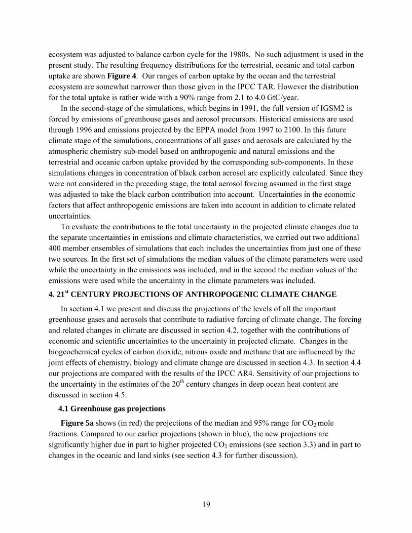
Figure 5a shows (in red) the projections of the median and 95% range for CO2 mole fractions. Compared to our earlier projections (shown in blue), the new projections are significantly higher due in part to higher projected CO2 emissions (see section 3.3) and in part to changes in the oceanic and land sinks (see section 4.3 for further discussion).

19

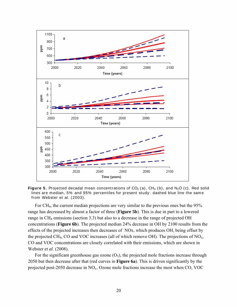
Figure 5. Projected decadal mean concentrations of CO2 (a), CH4 (b), and N2O (c). Red solid

lines are median, 5% and 95% percentiles for present study: dashed blue line the same from Webster et al. (2003).

For CH4, the current median projections are very similar to the previous ones but the 95% range has decreased by almost a factor of three (Figure 5b). This is due in part to a lowered range in CH4 emissions (section 3.3) but also to a decrease in the range of projected OH concentrations (Figure 6b). The projected median 24% decrease in OH by 2100 results from the effects of the projected increases then decreases of NOx, which produces OH, being offset by the projected CH4, CO and VOC increases (all of which remove OH). The projections of NOx, CO and VOC concentrations are closely correlated with their emissions, which are shown in Webster et al. (2008).

For the significant greenhouse gas ozone (O3), the projected mole fractions increase through 2050 but then decrease after that (red curves in Figure 6a). This is driven significantly by the projected post-2050 decrease in NOx. Ozone mole fractions increase the most when CO, VOC

20

and NOx mole fractions all increase together, but not when CO and VOC increases accompany NOx decreases.

Figure 6. Projected decadal mean concentrations of ozone (a), and OH radical (b). The

latter is shown as a ratio to its values averaged over years 1991-2000. Red solid lines are median, 5% and 95% percentiles for present study: dashed blue line the same from Webster et al. (2003).

Median nitrous oxide (N2O) mole fractions are projected to increase by about 50% by 2100 (Figure 5c) driven by increasing anthropogenic emissions (section 3.3) and increased natural emissions induced by projected increase in soil temperature, rainfall and soil labile carbon.

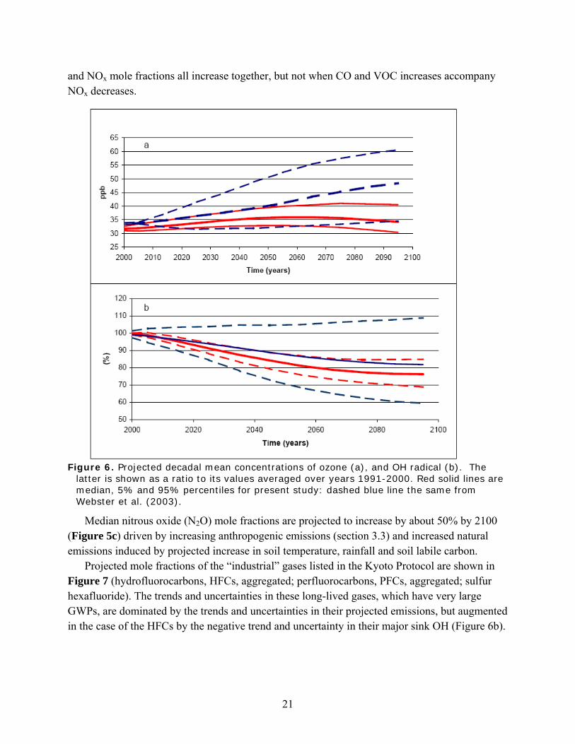
Projected mole fractions of the “industrial” gases listed in the Kyoto Protocol are shown in Figure 7 (hydrofluorocarbons, HFCs, aggregated; perfluorocarbons, PFCs, aggregated; sulfur hexafluoride). The trends and uncertainties in these long-lived gases, which have very large GWPs, are dominated by the trends and uncertainties in their projected emissions, but augmented in the case of the HFCs by the negative trend and uncertainty in their major sink OH (Figure 6b).

21

Figure 7. Changes in concentration of some GHGs averaged over 2041-2050 (a) and 2091-

2100 (b) relative to 1991-2000 in present study (new) and in Webster et al., (2003) (old). HFCs and SFC are reduced by factors 100 and 10, respectively. Radiative effect of changes in the concentration of black carbon was not taken into account in Webster et al. (2003).

Figure 7 also shows projections of mole fractions of SO2, which is the precursor for sulfate aerosols and has both anthropogenic and natural (dimethyl sulfide oxidation) sources. The median and range projections are driven primarily by the projected anthropogenic emissions, but augmented by the projected decrease and uncertainty in OH, which is the principal gas-phase sink for SO2 (converting it to sulfate aerosol).

22

Finally, black carbon projections are also shown in Figure 7. Like the SO2 projections, they are driven by the anthropogenic emissions but are not affected by OH. Their principal removal is instead through dry and wet deposition to the surface.

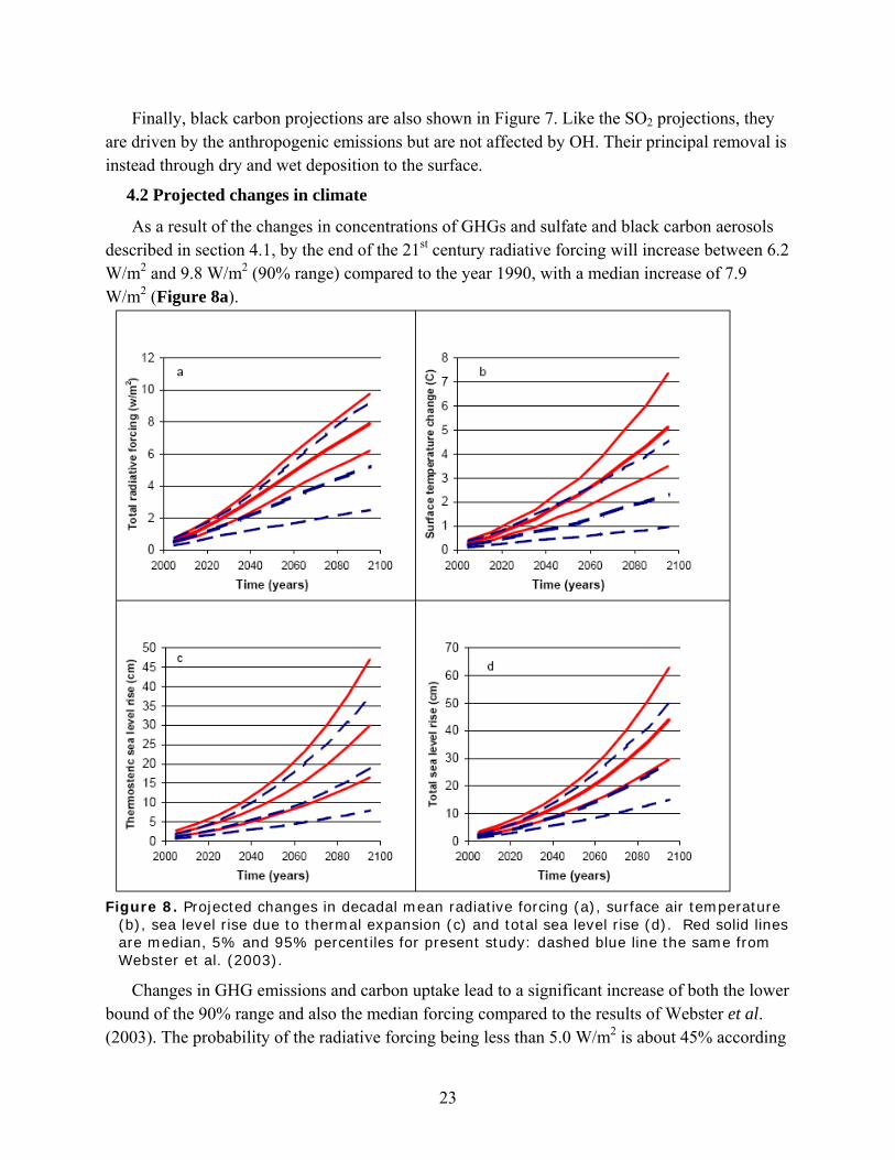
4.2 Projected changes in climate As a result of the changes in concentrations of GHGs and sulfate and black carbon aerosols

described in section 4.1, by the end of the 21st century radiative forcing will increase between 6.2 W/m2 and 9.8 W/m2 (90% range) compared to the year 1990, with a median increase of 7.9 W/m2 (Figure 8a).

Figure 8. Projected changes in decadal mean radiative forcing (a), surface air temperature

(b), sea level rise due to thermal expansion (c) and total sea level rise (d). Red solid lines are median, 5% and 95% percentiles for present study: dashed blue line the same from Webster et al. (2003).

Changes in GHG emissions and carbon uptake lead to a significant increase of both the lower bound of the 90% range and also the median forcing compared to the results of Webster et al. (2003). The probability of the radiative forcing being less than 5.0 W/m2 is about 45% according

23

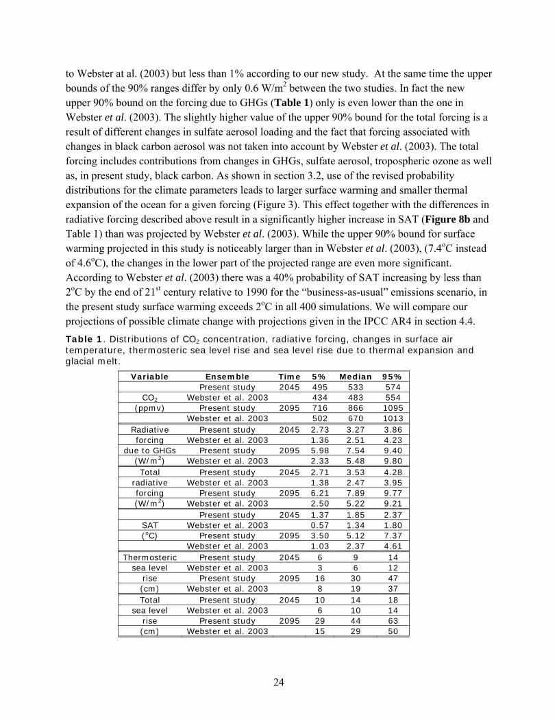
to Webster at al. (2003) but less than 1% according to our new study. At the same time the upper bounds of the 90% ranges differ by only 0.6 W/m2 between the two studies. In fact the new upper 90% bound on the forcing due to GHGs (Table 1) only is even lower than the one in Webster et al. (2003). The slightly higher value of the upper 90% bound for the total forcing is a result of different changes in sulfate aerosol loading and the fact that forcing associated with changes in black carbon aerosol was not taken into account by Webster et al. (2003). The total forcing includes contributions from changes in GHGs, sulfate aerosol, tropospheric ozone as well as, in present study, black carbon. As shown in section 3.2, use of the revised probability distributions for the climate parameters leads to larger surface warming and smaller thermal expansion of the ocean for a given forcing (Figure 3). This effect together with the differences in radiative forcing described above result in a significantly higher increase in SAT (Figure 8b and Table 1) than was projected by Webster et al. (2003). While the upper 90% bound for surface warming projected in this study is noticeably larger than in Webster et al. (2003), (7.4oC instead of 4.6oC), the changes in the lower part of the projected range are even more significant. According to Webster et al. (2003) there was a 40% probability of SAT increasing by less than 2oC by the end of 21st century relative to 1990 for the “business-as-usual” emissions scenario, in the present study surface warming exceeds 2oC in all 400 simulations. We will compare our projections of possible climate change with projections given in the IPCC AR4 in section 4.4. Table 1. Distributions of CO2 concentration, radiative forcing, changes in surface air temperature, thermosteric sea level rise and sea level rise due to thermal expansion and glacial melt.

Variable Ensemble Time 5% Median 95% Present study 2045 495 533 574

CO2 Webster et al. 2003 434 483 554 (ppmv) Present study 2095 716 866 1095

Webster et al. 2003 502 670 1013 Radiative Present study 2045 2.73 3.27 3.86 forcing Webster et al. 2003 1.36 2.51 4.23

due to GHGs Present study 2095 5.98 7.54 9.40 (W/m2) Webster et al. 2003 2.33 5.48 9.80 Total Present study 2045 2.71 3.53 4.28

radiative Webster et al. 2003 1.38 2.47 3.95 forcing Present study 2095 6.21 7.89 9.77 (W/m2) Webster et al. 2003 2.50 5.22 9.21

Present study 2045 1.37 1.85 2.37 SAT Webster et al. 2003 0.57 1.34 1.80 (oC) Present study 2095 3.50 5.12 7.37

Webster et al. 2003 1.03 2.37 4.61 Thermosteric Present study 2045 6 9 14

sea level Webster et al. 2003 3 6 12 rise Present study 2095 16 30 47 (cm) Webster et al. 2003 8 19 37 Total Present study 2045 10 14 18

sea level Webster et al. 2003 6 10 14 rise Present study 2095 29 44 63 (cm) Webster et al. 2003 15 29 50

24

From the above mentioned decrease in the thermal expansion of the ocean for a given forcing (Figure 3b) and the similarity of the upper 90% bounds of forcing (Figure 8a), one might expect the upper limit of the thermosteric sea level rise to be smaller in the present study than in Webster et al. (2003). However, this is not the case1 (Figure 8c). This apparent contradiction is explained by the changes in the ocean carbon model. As shown by Sokolov et al. (1998), the assumed dependency between rates of heat and carbon uptake by the ocean imposes a negative correlation between the rate of heat mixing into the deep ocean and the atmospheric CO2 concentration, which leads to a decrease in the uncertainty range for thermal expansion. Changes in the parameterization of oceanic carbon uptake in the current model (see section 2.3 and Sokolov et al. 2007) weakened this correlation, resulting in a wider range of the thermosteric sea level rise. The differences between the two studies in projected sea level rise, especially in the component related to the thermal expansion of the deep ocean, are, however, relatively smaller than the differences in projected surface temperature (Figure 8).

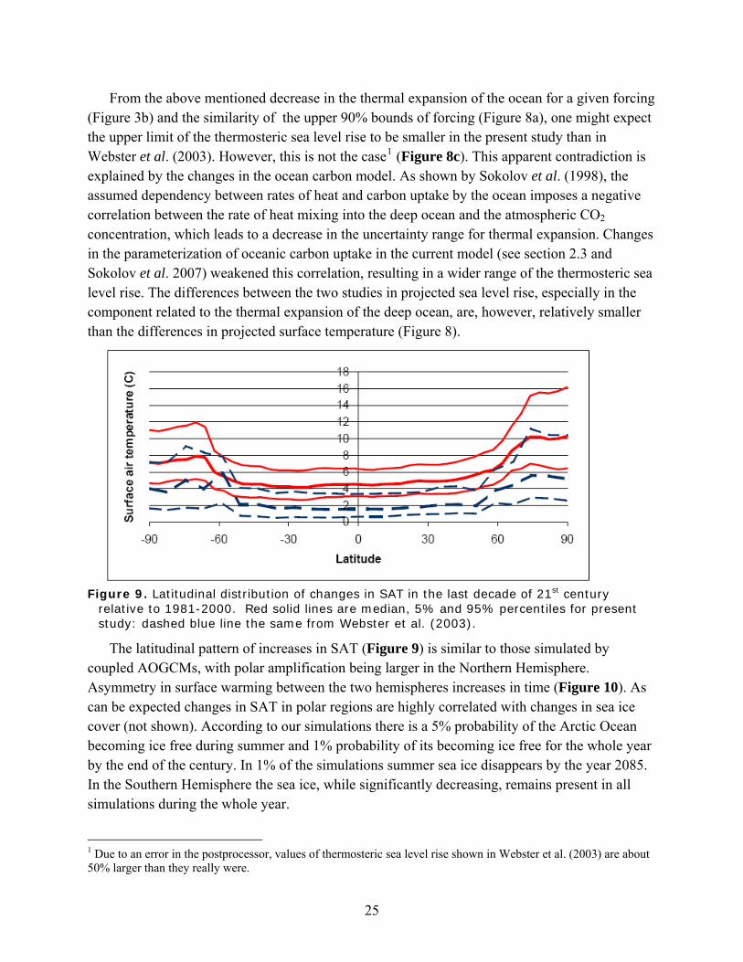
Figure 9. Latitudinal distribution of changes in SAT in the last decade of 21st century

relative to 1981-2000. Red solid lines are median, 5% and 95% percentiles for present study: dashed blue line the same from Webster et al. (2003).

The latitudinal pattern of increases in SAT (Figure 9) is similar to those simulated by coupled AOGCMs, with polar amplification being larger in the Northern Hemisphere. Asymmetry in surface warming between the two hemispheres increases in time (Figure 10). As can be expected changes in SAT in polar regions are highly correlated with changes in sea ice cover (not shown). According to our simulations there is a 5% probability of the Arctic Ocean becoming ice free during summer and 1% probability of its becoming ice free for the whole year by the end of the century. In 1% of the simulations summer sea ice disappears by the year 2085. In the Southern Hemisphere the sea ice, while significantly decreasing, remains present in all simulations during the whole year.

1 Due to an error in the postprocessor, values of thermosteric sea level rise shown in Webster et al. (2003) are about 50% larger than they really were.

25

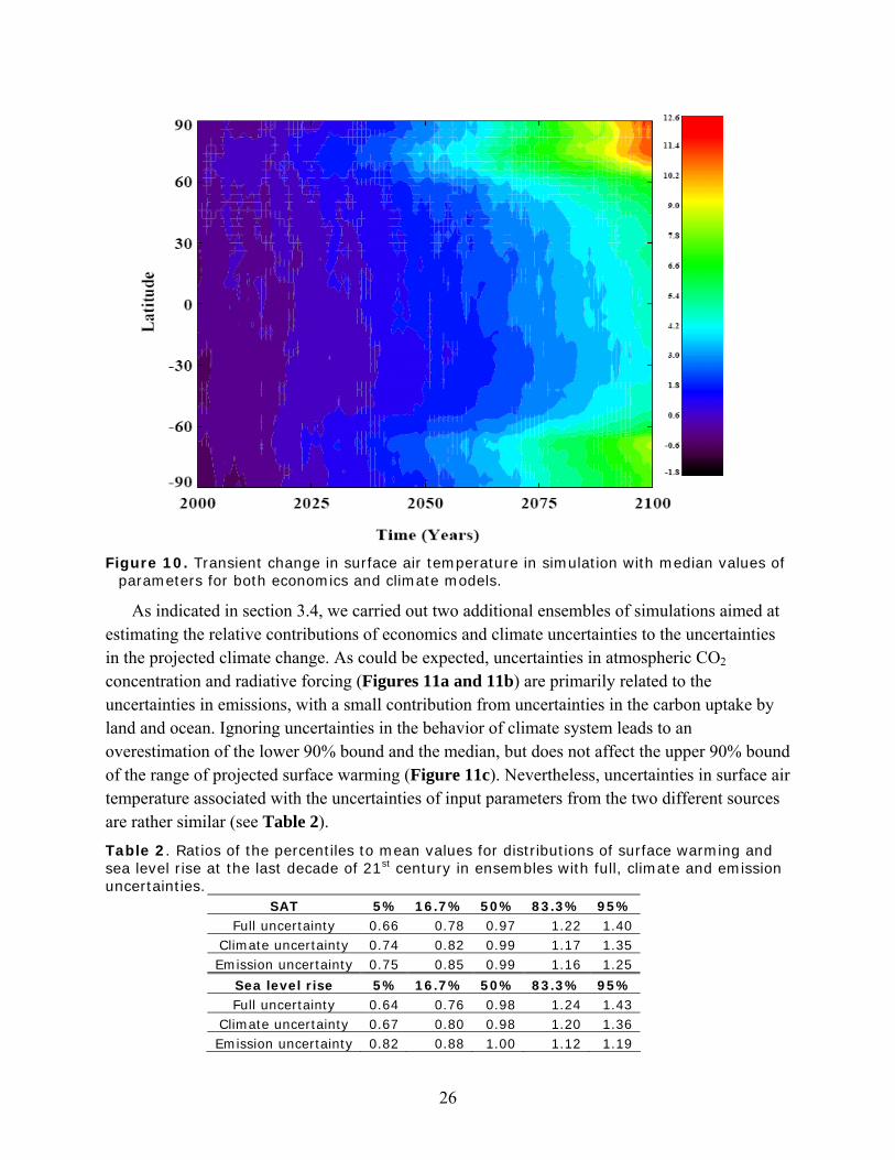
Figure 10. Transient change in surface air temperature in simulation with median values of

parameters for both economics and climate models.

As indicated in section 3.4, we carried out two additional ensembles of simulations aimed at estimating the relative contributions of economics and climate uncertainties to the uncertainties in the projected climate change. As could be expected, uncertainties in atmospheric CO2 concentration and radiative forcing (Figures 11a and 11b) are primarily related to the uncertainties in emissions, with a small contribution from uncertainties in the carbon uptake by land and ocean. Ignoring uncertainties in the behavior of climate system leads to an overestimation of the lower 90% bound and the median, but does not affect the upper 90% bound of the range of projected surface warming (Figure 11c). Nevertheless, uncertainties in surface air temperature associated with the uncertainties of input parameters from the two different sources are rather similar (see Table 2). Table 2. Ratios of the percentiles to mean values for distributions of surface warming and sea level rise at the last decade of 21st century in ensembles with full, climate and emission uncertainties.

SAT 5% 16.7% 50% 83.3% 95% Full uncertainty 0.66 0.78 0.97 1.22 1.40

Climate uncertainty 0.74 0.82 0.99 1.17 1.35 Emission uncertainty 0.75 0.85 0.99 1.16 1.25

Sea level rise 5% 16.7% 50% 83.3% 95% Full uncertainty 0.64 0.76 0.98 1.24 1.43

Climate uncertainty 0.67 0.80 0.98 1.20 1.36 Emission uncertainty 0.82 0.88 1.00 1.12 1.19

26

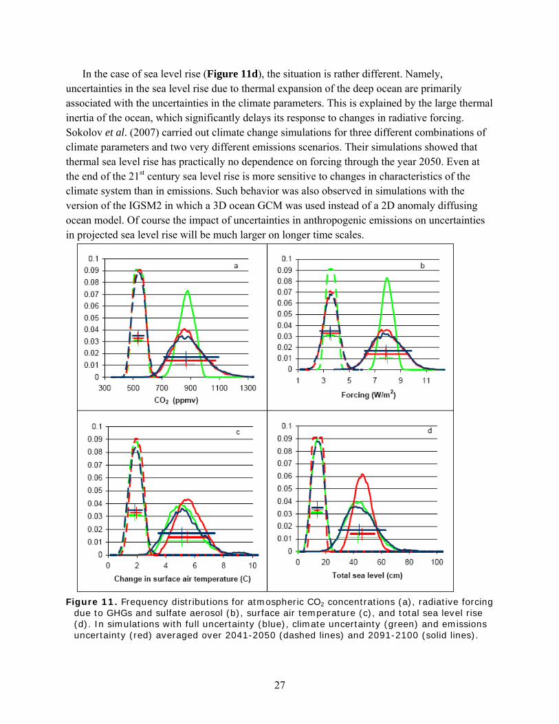
In the case of sea level rise (Figure 11d), the situation is rather different. Namely, uncertainties in the sea level rise due to thermal expansion of the deep ocean are primarily associated with the uncertainties in the climate parameters. This is explained by the large thermal inertia of the ocean, which significantly delays its response to changes in radiative forcing. Sokolov et al. (2007) carried out climate change simulations for three different combinations of climate parameters and two very different emissions scenarios. Their simulations showed that thermal sea level rise has practically no dependence on forcing through the year 2050. Even at the end of the 21st century sea level rise is more sensitive to changes in characteristics of the climate system than in emissions. Such behavior was also observed in simulations with the version of the IGSM2 in which a 3D ocean GCM was used instead of a 2D anomaly diffusing ocean model. Of course the impact of uncertainties in anthropogenic emissions on uncertainties in projected sea level rise will be much larger on longer time scales.

Figure 11. Frequency distributions for atmospheric CO2 concentrations (a), radiative forcing

due to GHGs and sulfate aerosol (b), surface air temperature (c), and total sea level rise (d). In simulations with full uncertainty (blue), climate uncertainty (green) and emissions uncertainty (red) averaged over 2041-2050 (dashed lines) and 2091-2100 (solid lines).

27

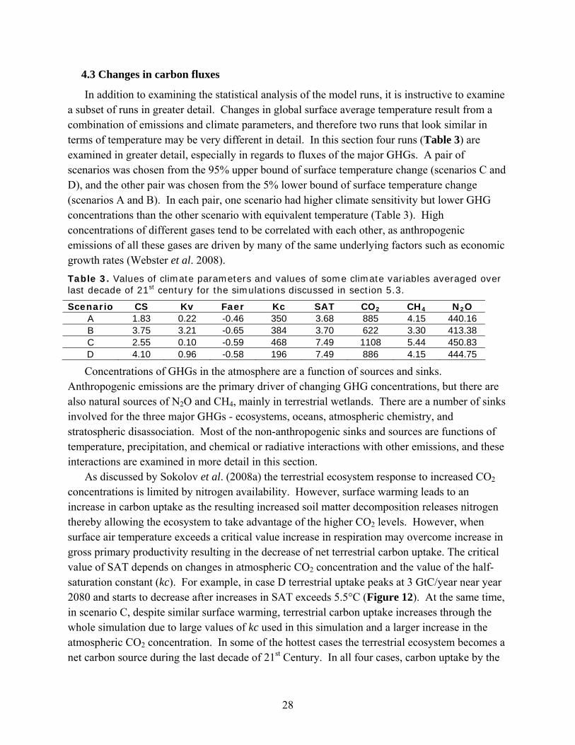
4.3 Changes in carbon fluxes In addition to examining the statistical analysis of the model runs, it is instructive to examine

a subset of runs in greater detail. Changes in global surface average temperature result from a combination of emissions and climate parameters, and therefore two runs that look similar in terms of temperature may be very different in detail. In this section four runs (Table 3) are examined in greater detail, especially in regards to fluxes of the major GHGs. A pair of scenarios was chosen from the 95% upper bound of surface temperature change (scenarios C and D), and the other pair was chosen from the 5% lower bound of surface temperature change (scenarios A and B). In each pair, one scenario had higher climate sensitivity but lower GHG concentrations than the other scenario with equivalent temperature (Table 3). High concentrations of different gases tend to be correlated with each other, as anthropogenic emissions of all these gases are driven by many of the same underlying factors such as economic growth rates (Webster et al. 2008). Table 3. Values of climate parameters and values of some climate variables averaged over last decade of 21st century for the simulations discussed in section 5.3.

Scenario CS Kv Faer Kc SAT CO2 CH4 N2O A 1.83 0.22 -0.46 350 3.68 885 4.15 440.16 B 3.75 3.21 -0.65 384 3.70 622 3.30 413.38 C 2.55 0.10 -0.59 468 7.49 1108 5.44 450.83 D 4.10 0.96 -0.58 196 7.49 886 4.15 444.75

Concentrations of GHGs in the atmosphere are a function of sources and sinks. Anthropogenic emissions are the primary driver of changing GHG concentrations, but there are also natural sources of N2O and CH4, mainly in terrestrial wetlands. There are a number of sinks involved for the three major GHGs - ecosystems, oceans, atmospheric chemistry, and stratospheric disassociation. Most of the non-anthropogenic sinks and sources are functions of temperature, precipitation, and chemical or radiative interactions with other emissions, and these interactions are examined in more detail in this section.

As discussed by Sokolov et al. (2008a) the terrestrial ecosystem response to increased CO2 concentrations is limited by nitrogen availability. However, surface warming leads to an increase in carbon uptake as the resulting increased soil matter decomposition releases nitrogen thereby allowing the ecosystem to take advantage of the higher CO2 levels. However, when surface air temperature exceeds a critical value increase in respiration may overcome increase in gross primary productivity resulting in the decrease of net terrestrial carbon uptake. The critical value of SAT depends on changes in atmospheric CO2 concentration and the value of the half-saturation constant (kc). For example, in case D terrestrial uptake peaks at 3 GtC/year near year 2080 and starts to decrease after increases in SAT exceeds 5.5°C (Figure 12). At the same time, in scenario C, despite similar surface warming, terrestrial carbon uptake increases through the whole simulation due to large values of kc used in this simulation and a larger increase in the atmospheric CO2 concentration. In some of the hottest cases the terrestrial ecosystem becomes a net carbon source during the last decade of 21st Century. In all four cases, carbon uptake by the

28

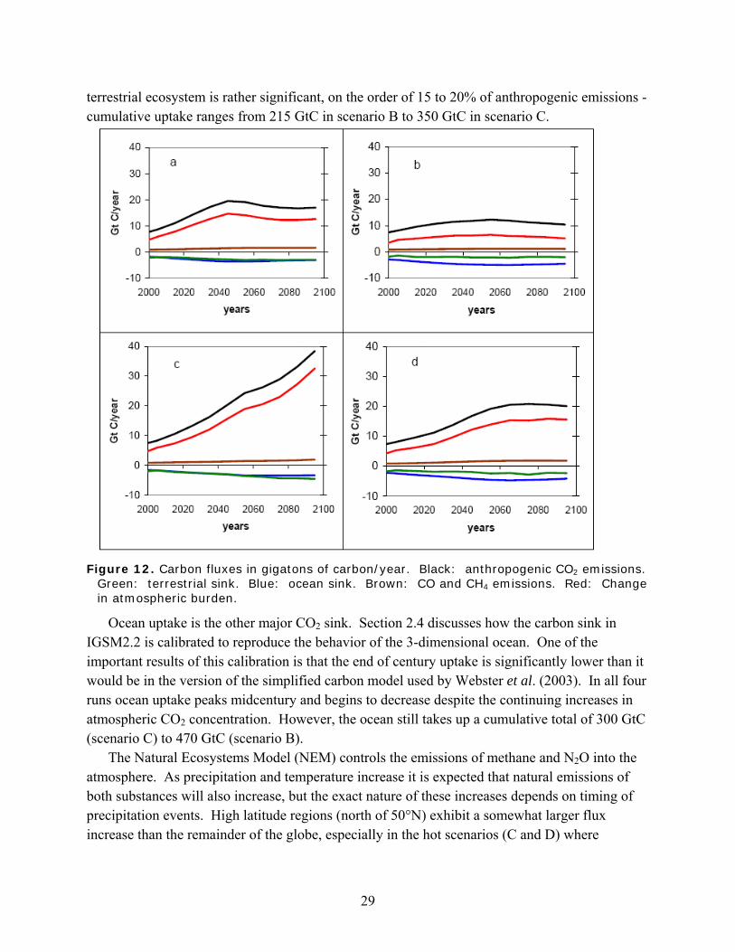
terrestrial ecosystem is rather significant, on the order of 15 to 20% of anthropogenic emissions - cumulative uptake ranges from 215 GtC in scenario B to 350 GtC in scenario C.

Figure 12. Carbon fluxes in gigatons of carbon/year. Black: anthropogenic CO2 emissions.

Green: terrestrial sink. Blue: ocean sink. Brown: CO and CH4 emissions. Red: Change in atmospheric burden.

Ocean uptake is the other major CO2 sink. Section 2.4 discusses how the carbon sink in IGSM2.2 is calibrated to reproduce the behavior of the 3-dimensional ocean. One of the important results of this calibration is that the end of century uptake is significantly lower than it would be in the version of the simplified carbon model used by Webster et al. (2003). In all four runs ocean uptake peaks midcentury and begins to decrease despite the continuing increases in atmospheric CO2 concentration. However, the ocean still takes up a cumulative total of 300 GtC (scenario C) to 470 GtC (scenario B).

The Natural Ecosystems Model (NEM) controls the emissions of methane and N2O into the atmosphere. As precipitation and temperature increase it is expected that natural emissions of both substances will also increase, but the exact nature of these increases depends on timing of precipitation events. High latitude regions (north of 50°N) exhibit a somewhat larger flux increase than the remainder of the globe, especially in the hot scenarios (C and D) where

29

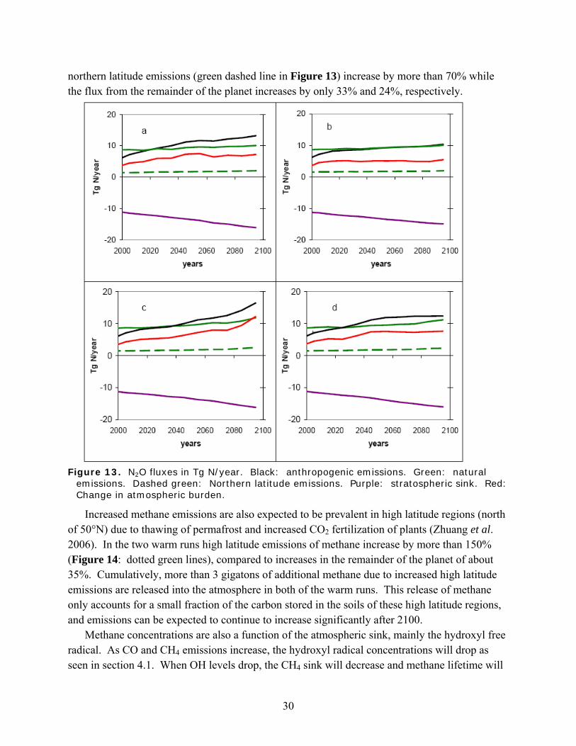
northern latitude emissions (green dashed line in Figure 13) increase by more than 70% while the flux from the remainder of the planet increases by only 33% and 24%, respectively.

Figure 13. N2O fluxes in Tg N/year. Black: anthropogenic emissions. Green: natural

emissions. Dashed green: Northern latitude emissions. Purple: stratospheric sink. Red: Change in atmospheric burden.

Increased methane emissions are also expected to be prevalent in high latitude regions (north of 50°N) due to thawing of permafrost and increased CO2 fertilization of plants (Zhuang et al. 2006). In the two warm runs high latitude emissions of methane increase by more than 150% (Figure 14: dotted green lines), compared to increases in the remainder of the planet of about 35%. Cumulatively, more than 3 gigatons of additional methane due to increased high latitude emissions are released into the atmosphere in both of the warm runs. This release of methane only accounts for a small fraction of the carbon stored in the soils of these high latitude regions, and emissions can be expected to continue to increase significantly after 2100.

Methane concentrations are also a function of the atmospheric sink, mainly the hydroxyl free radical. As CO and CH4 emissions increase, the hydroxyl radical concentrations will drop as seen in section 4.1. When OH levels drop, the CH4 sink will decrease and methane lifetime will

30

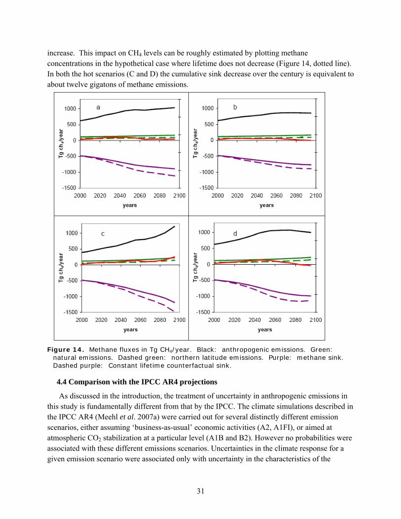
increase. This impact on CH4 levels can be roughly estimated by plotting methane concentrations in the hypothetical case where lifetime does not decrease (Figure 14, dotted line). In both the hot scenarios (C and D) the cumulative sink decrease over the century is equivalent to about twelve gigatons of methane emissions.

Figure 14. Methane fluxes in Tg CH4/year. Black: anthropogenic emissions. Green:

natural emissions. Dashed green: northern latitude emissions. Purple: methane sink. Dashed purple: Constant lifetime counterfactual sink.

4.4 Comparison with the IPCC AR4 projections

As discussed in the introduction, the treatment of uncertainty in anthropogenic emissions in this study is fundamentally different from that by the IPCC. The climate simulations described in the IPCC AR4 (Meehl et al. 2007a) were carried out for several distinctly different emission scenarios, either assuming ‘business-as-usual’ economic activities (A2, A1FI), or aimed at atmospheric CO2 stabilization at a particular level (A1B and B2). However no probabilities were associated with these different emissions scenarios. Uncertainties in the climate response for a given emission scenario were associated only with uncertainty in the characteristics of the

31

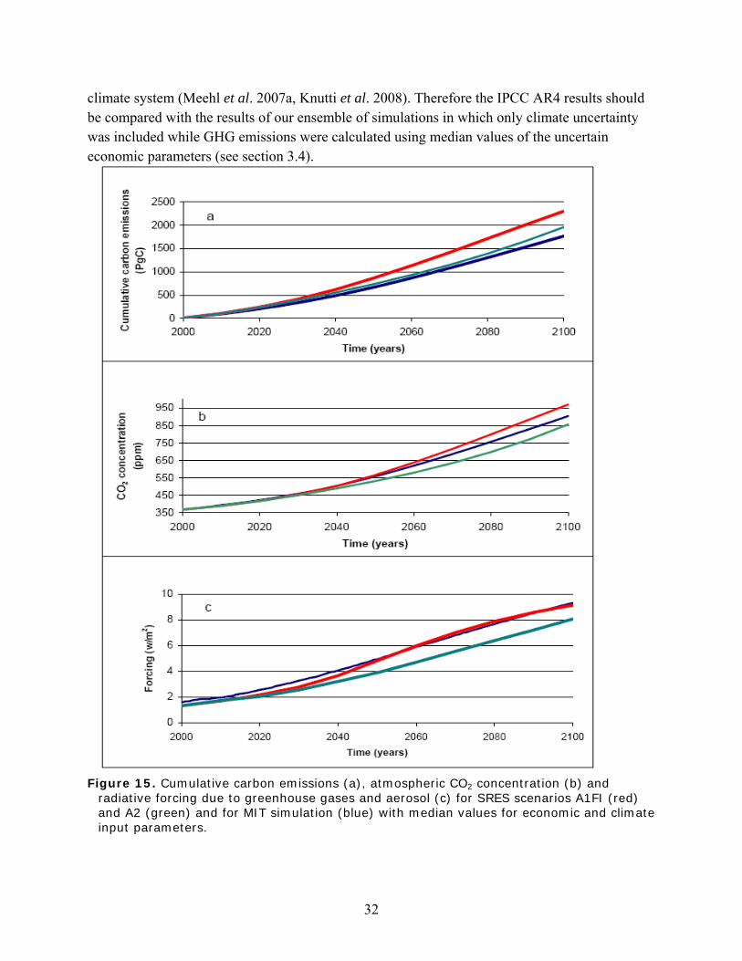
climate system (Meehl et al. 2007a, Knutti et al. 2008). Therefore the IPCC AR4 results should be compared with the results of our ensemble of simulations in which only climate uncertainty was included while GHG emissions were calculated using median values of the uncertain economic parameters (see section 3.4).

Figure 15. Cumulative carbon emissions (a), atmospheric CO2 concentration (b) and

radiative forcing due to greenhouse gases and aerosol (c) for SRES scenarios A1FI (red) and A2 (green) and for MIT simulation (blue) with median values for economic and climate input parameters.

32

The cumulative carbon emissions produced by the EPPA model with these parameter values are very similar to those for the A2 scenario and somewhat smaller than those in the A1FI scenario (see Figure 15a). However, the atmospheric CO2 concentration obtained in the simulation with the IGSM using the median values of both the emission and climate parameters is closer to the concentration in the A1FI scenario (Figure 15b). This is explained, at least partly, by the fact that the terrestrial ecosystem model used in the IGSM2, in contrast to the ISAM model used to calculate CO2 concentrations for the SRES scenarios, considers carbon/nitrogen interactions. As shown by Sokolov et al (2008a), taking into account the nitrogen limitation on terrestrial carbon uptake leads to a large increase in atmospheric CO2 for given carbon emissions. The forcings due to individual GHGs (CH4, N2O, etc.) are somewhat different for our median emission scenario and for A1FI, but the total forcings are quite similar (Figure 15c). Thus it is appropriate to compare our results for the ensemble of simulations including only the climate model uncertainties with the IPCC’s projections for the A1FI scenario. More detailed comparison between MIT and SRES scenarios is given by Prinn et al. (2008).

Since the AR4 AOGCMs did not simulate the A1FI scenario, the IPCC calculated the mean value of SAT increase for the A1FI scenario from 19 simulations with the Simple Climate Model (SCM MAGGIC, Wigley and Raper, 2001). The 19 different versions of the SCM were each tuned to simulate the behavior of a different one of the 19 AOGCMs used in the IPCC AR4 (Meehl et al. 2007a). The mean of the 19 SCM simulations was scaled to allow for a small bias in the SCM compared to the AOGCMs simulations for other scenarios (Meehl et al. 2007a, Knutti et al. 2008). Because, as noted by Meehl et al. (2007a), AOGCMs do not sample the full range of possible warming, the IPCC AR4’s projected likely range (Solomon et al. 2007) of warming is not based solely on the 19 simulations but was estimated with the help of results of additional studies (Knutti et al. 2008), including simulations with models of intermediate complexity. Some of the models of intermediate complexity in addition to uncertainties in climate sensitivity, rate of oceanic heat uptake, strength of aerosol forcing and carbon cycle consider uncertainty in the feedback between the carbon cycle and climate (e.g. Knutti et al. 2003). Thus the likely range of warming was judged to extend from 40% less to 60% more than the mean SAT increase (Meehl et al. 2007a, Knutti et al. 2008). We note that, according to the IPCC AR4 definition, the probability of SAT change falling into the likely range is more than 66% but less than 90%. Table 4. Change is SAT at the last decade of 21st century relative to 1981-2000, at year 2100 for Meinshausen et al (2008)

5% 16.7% Mean 83.3% 95% MIT simulations with median anthropogenic emissions 3.81 4.22 5.17 6.04 6.98 Meinshausen et al (2008) (with uncertainty in feedback between climate and carbon cycle) for SRES A1FI

2.85 3.26 4.09 4.79 5.88

SCM MAGIC (with carbon uptake uncertainty) for SRES A1FI

3.30 4.40 5.80

IPCC AR4 for SRES A1FI 2.40 4.00 6.40

33

Table 4 compares the IPCC's mean and likely range of SAT increase for the A1FI scenario with those based on the results of the simulations with the latest version of the SCM MAGIC (Meinshausen et al 2008), tuned to 19 AR4 AOGCMs, and with those from our simulations with median anthropogenic emissions.

As discussed by Sokolov et al (2008b), the AR4 multi-model ensemble underestimate surface warming compared to MIT simulations with input parameters distributions obtained using Levitus et al. (2005) data on changes in deep ocean heat content. The same, of course, is true for the SCM MAGIC. In particular, our mean SAT increase is 30% greater than the IPCC's. The uncertainty range obtained in the MIT simulations is both narrower and more symmetric than the range given by the IPC. i.e., the lower bound of the 90% range is smaller than the mean by 26% while the upper bound is larger by 35% (Table 5). The asymmetry in the IPCC range is, to a large extent, associated with the uncertainty in the carbon cycle/climate feedback. As indicated by Knutti et al. (2008), inclusion of the uncertainty in carbon cycle/climate feedback as simulated by the C4MIP models (Friedlingstein et al. 2006) extends the projected range of surface warming, with larger effect on the upper bound. In contrast with all models used by the IPCC the MIT IGSM takes into account the carbon/nitrogen interaction in the terrestrial ecosystem. As was shown by Sokolov et al. (2008a), considering this interaction significantly reduces the strength of the feedback between the carbon cycle and climate and the uncertainty in the projected CO2 concentration and surface warming associated with this feedback. Table 5. Ratios of the percentiles values to the means for probability distributions shown in Table 4.

5% 16.7% 83.3% 95% MIT simulations with median anthropogenic emissions 0.74 0.82 1.17 1.35 Meinshausen et al (2008) (with uncertainty in feedback between climate and carbon cycle) for SRES A1FI

0.70 0.80 1.17 1.44

SCM MAGIC (with carbon uptake uncertainty) for SRES A1FI

0.77 1.35

IPCC AR4 for SRES A1FI 0.60 1.60

4.5 Sensitivity of the projected surface warming to the deep-ocean data used to derive climate input parameters

Sokolov et al. (2008b) compared results of ensembles of projections with the climate component of the MIT IGSM carried out using distributions of climate input parameters obtained with different data for changes in deep ocean heat content. As noted in the introduction, for the comparison with our previous results (Webster et al. 2003), we decided to use climate parameter distributions based on the Levitus et al. (2005) data in our simulations. We refer to these distributions as the LEV05 distributions. However, results presented by Sokolov et al. (2008b) allow us to approximate the distribution of changes in SAT for different climate parameter distributions without running a full ensemble of simulations. In this section we show how our results would have changed if we have had used input distributions for climate parameters based either on Domingous et al. (2008) or on upper and surface air temperatures only, DOM08 and

34

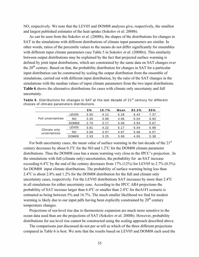
NO, respectively. We note that the LEV05 and DOM08 analyses give, respectively, the smallest and largest published estimates of the heat uptake (Sokolov et al. 2008b).

As can be seen from the Sokolov et al. (2008b), the shapes of the distributions for changes in SAT in the simulations with different distributions of climate input parameters are similar. In other words, ratios of the percentile values to the means do not differ significantly for ensembles with different input climate parameters (see Table 5 in Sokolov et al. (2008b)). This similarity between output distributions may be explained by the fact that projected surface warming is defined by joint input distributions, which are constrained by the same data on SAT changes over the 20th century. Based on that, the probability distribution for changes in SAT for a particular input distribution can be constructed by scaling the output distribution from the ensemble of simulations, carried out with different input distribution, by the ratio of the SAT changes in the simulations with the median values of input climate parameters from the two input distributions. Table 6 shows the alternative distributions for cases with climate only uncertainty and full uncertainty. Table 6. Distributions for changes in SAT at the last decade of 21st century for different choices of climate parameters distributions.

5% 16.7% Mean 83.3% 95% LEV05 3.50 4.12 5.28 6.42 7.37

NO 3.30 3.88 4.96 6.04 6.93 Full uncertainties

DOM08 2.70 3.17 4.06 4.94 5.67 LEV05 3.81 4.22 5.17 6.04 6.98

NO 3.58 3.97 4.87 5.68 6.57 Climate only uncertainties

DOM08 2.93 3.25 3.98 4.65 5.38

For both uncertainty cases, the mean value of surface warming in the last decade of the 21st century decreases by about 0.3oC for the NO and 1.2oC for the DOM08 climate parameter distributions. Thus the DOM08 case has a mean warming very close to the IPCC’s projection. .In the simulations with full (climate only) uncertainties, the probability for an SAT increase exceeding 6.4oC by the end of the century decreases from 17% (12%) for LEV05 to 2.7% (0.5%) for DOM08 input climate distributions. The probability of surface warming being less than 2.4oC is about 2.8% and 1.2% for the DOM08 distribution for the full and climate only uncertainty cases, respectively. For the LEV05 distributions SAT increases by more than 2.4oC in all simulations for either uncertainty case. According to the IPCC AR4 projections the probability of SAT increase larger than 6.4oC or smaller than 2.4oC for theA1FI scenario is estimated as being between 5% and 16.7%. The much smaller likelihood we find for modest warming is likely due to our input pdfs having been explicitly constrained by 20th century temperature changes.

Projections of sea-level rise due to thermosteric expansion are much more sensitive to the ocean data used than are the projections of SAT (Sokolov et al. 2008b). However, probability distributions for sea level rise cannot be constructed using the scaling approach described above.

The comparisons just discussed do not per se tell us which of the three different projections compared in Table 6 is best. We note that the results based on LEV05 and DOM08 each used the

35

error estimates given by the respective analyses as being appropriate for their estimates of the trend in ocean warming. However these estimates are mutually incompatible. The DOM85 trend is more than double the LEV05 trend, but the difference between the two trends is five/seven times the standard deviation in the trend cited by the respective analyses. All this emphasizes an urgent necessity for obtaining more definite estimates for changes in deep-ocean heat content.

5. CONCLUSIONS

In this paper we have presented updated projections of climate changes for the 21st century in the absence of any climate policy. While the MIT IGSM has been significantly modified since publication of our previous projections (Webster et al. 2003), the primary reasons for the differences between our previous and present results are changes in the distributions of input parameters for both the earth system and economic components of the IGSM.

The simulations of 20th century climate used to estimate uncertainties in the climate system parameters (Forest et al. 2006 and 2008) were carried out using both anthropogenic and natural forcings. As discussed by Forest et al. (2006), taking into account natural forcings, especially forcing due to volcanic eruptions, led to significantly different distributions of climate system parameters compared to the distributions based on 20th century simulations with just anthropogenic forcings (Forest et al. 2002), which was used by Webster et al. (2003). The main consequence of the changes in the climate input distributions is an increase in the lower bound of the distribution of surface warming in response to an external forcing.

Similarly, the distributions of global GHGs emissions used in this study (Webster et al. 2008) are higher, compared with previous results (Webster et al. 2002) due to the reduction of very low emissions growth cases. One of the key differences is that GDP growth, while still more important than many other parameters, is not the primary driver of uncertainty in emissions. This change is a result of the new approach of generating GDP growth paths using a random walk, and of the assumption that GDP growth shocks are not correlated across countries. From this analysis, the primary drivers of uncertainty in no-policy carbon emissions are technological change, both price driven (e.g., elasticity of substitution) and non-price driven (e.g., autonomous energy efficiency improvement), and the total fossil resources available, particularly coal and shale (Webster et al. 2008). These changes in projected GHGs emissions noticeably decreased the probability of low radiative forcing.

Due to the multiplicative nature of the interaction between the forcing and the climate system response, the probability distribution of the increase in surface air temperature at the end of the 21st century is shifted upward significantly compared to the distribution obtained by Webster et al. (2003). As can be expected from the changes in the forcing and the response described above, the biggest difference is a sharp decrease in the probability of small or moderate warming. While the upper bound of the 90% range has increased by about 60%, the lower bound of the 90% range of the new distribution is more than 3 times larger than in the Webster et al. (2003).

While our median anthropogenic emissions are similar to those for the SRES A2 scenario, the GHGs concentrations simulated by the MIT IGSM are somewhat higher than those used in

36

the simulations with the IPCC AR4 AOGCMs. These differences in GHG concentrations arise from the different treatment of the terrestrial ecosystem and from the fact that we take into account an increase in the natural CH4 and N2O emissions caused by the surface warming, as well as from differences in chemistry models (Prinn et al. 2008). As a result, the total radiative forcing in our simulations with median anthropogenic emissions is quite close to the forcing for the IPCC A1FI scenario. However, the surface warming projected by the MIT IGSM significantly exceeds the estimates given by Meehl et al. (2007a). The shape of the probability distribution of changes in SAT simulated by the MIT IGSM is also different from that assumed by the IPCC AR4. The distribution obtained in our simulations is almost symmetric while the IPCC’s distribution implies a long upper tail. Asymmetry in the IPCC distribution is, in part, explained by the larger impact of the uncertainty in the feedback between the climate and the carbon cycle on the upper bound of the surface warming range. Taking into consideration the interaction between carbon and nitrogen in the terrestrial ecosystem model reduces the strength of this feedback and the uncertainty in surface warming associated with it (Sokolov et al. 2008a).

All the ensembles of simulations presented in this paper were carried out with climate input parameter distributions based on the Levitus et al. (2005) estimate of changes in the deep ocean heat content. We also derived approximate distributions of changes in SAT for climate parameter distributions based on alternate estimates of the ocean heat uptake. These estimates suggest somewhat smaller surface warming. However, the probability of the SAT increase at the end of the 21st century being near 2oC-2.5oC is significantly lower than that suggested by the IPCC AR4 for all the distributions tested.

Acknowledgments We would to thank Malte Meinshausen for providing results of the simulations with SCM MAGIC version 6 and Reto Knutii for useful discussion of SCM results. This work was supported in part by the Office of Science (BER), U.S. Department of Energy Grant No. DE-FG02-93ER61677, NSF, and by the MIT Joint Program on the Science and Policy of Global Change. We thank Josh Willis for discussions on the ocean heat content data. We acknowledge the modeling groups, the Program for Climate Model Diagnosis and Intercomparison (PCMDI) and the WCRP’s Working Group on Coupled Modelling (WGCM) for their roles in making available the WCRP CMIP3 multi-model dataset. Support of this dataset is provided by the Office of Science, U.S. Department of Energy.

6. REFERENCES Babiker, M.H., J.M. Reilly, M. Mayer, R.S. Eckaus, I. Sue Wing, and R.C. Hyman, 2001: The

MIT Emissions Prediction and Policy Analysis (EPPA) Model: Revisions, Sensitivities, and Comparisons of Results. MIT Joint Program on the Science and Policy of Global Change, Report 71, 90 pp, (Available on line at: http://web.mit.edu/globalchange/www/MITJPSPGC_Rpt71.pdf )

Babiker, M.H., G.E. Metcalf, and J. Reilly 2003: Tax distortions and global climate policy, Journal of Environmental Economics and Management, 46, 269-287.

Bonan, G.B., K.W. Oleson, M. Vertenstein, S. Lewis, X. Zeng, Y. Dai, R.E. Dickinson, and Z.-

37

L. Yang, 2002: The land surface climatology of the Community Land Model coupled to the NCAR Community Climate Model. J. Climate, 15, 3123-3149.

Calbó, J., W. Pan, M. Webster, R.G. Prinn, and G.J. McRae, 1998: Parameterization of urban sub-grid scale processes in global atmospheric chemistry models. J. Geophysical Research, 103, 3437-3451.

Curtis, P.S., and X. Wang, 1998: A meta-analysis of elevated CO2 effects on woody plant mass, form, and physiology. Oecologia, 113, 299-313.

Dalan, F., P.H. Stone, I. Kamenkovich, and J. Scott, 2005a: Sensitivity of the ocean’s climate to diapycnal diffusivity in EMIC. Part I: Equilibrium state. J. Climate, 18, 2460-2481.

Dalan, F., P.H. Stone, and A.P. Sokolov, 2005b: Sensitivity of the ocean’s climate to diapycnal diffusivity in EMIC. Part II: Global warming scenario. J. Climate, 18, 2482-2496.

Dimaranan, B., and R. McDougall, 2002: Global Trade, Assistance, and Production: The GTAP 5 Data Base. Center for Global Trade Analysis, Purdue University, West Lafayette, Indiana.

Domingues, C.M., J.A. Church, N.J. White, P.J. Gleckler, S.E. Wijffels, P.M. Barker, and J. R. Dunn, 2008: Improved estimates of upper-ocean warming and multi-decadal sea-level rise. Nature, 453, 1090-1094.

Edmonds, J. A., and J.M. Reilly, 1985: Future global energy and carbon dioxide emissions. Chapter 9 in Atmospheric Carbon Dioxide and the Global Carbon Cycle, (J. Trabalka, ed.), US Department of Energy, Office of Energy Research, DOE/ER-0239, Washington DC: 215-246.

Felzer, B., J. Reilly, J. Melillo, D. Kicklighter, M. Sarofim, C. Wang, R. Prinn, and Q. Zhuang, 2005: Future effects of ozone on carbon sequestration and climate change policy using a global biogeochemical model. Climatic Change, 73, 345-373.

Felzer, B., D.W. Kicklighter, J.M. Melillo, C. Wang, Q. Zhuang, and R. Prinn, 2004: Effects of ozone on net primary production and carbon sequestration in the conterminous United States using a biogeochemistry model. Tellus , 56B, 230-248.

Follows, M.J., T. Ito, and S. Dutkiewicz, 2006: A Compact and Accurate Carbonate Chemistry Solver for Ocean Biogeochemistry Models. Ocean Model, 12, 290-301.

Forest, C.E., P.H. Stone and A.P. Sokolov, 2008: Constraining Climate Model Parameters from Observed 20th Century Changes. Tellus, 60A, 911-920.

Forest, C.E., P.H. Stone, and A.P. Sokolov, 2006: Estimated PDFs of Climate System Properties Including Natural and Anthropogenic Forcings. Geophys. Res. Lett., 33, L01705, http://dx.doi.org/doi:10.1029/2005GL023977.

Forest, C.E., P.H. Stone, A.P. Sokolov, M.R. Allen, and M. Webster, 2002: Quantifying uncertainties in climate system properties with the use of recent climate observations. Science, 295, 113-117.

Friedlingstein, P., P. Cox, R. Betts, L. Bopp, W. von Bloh, V. Brovkin, P. Cadule, S. Doney, M. Eby, I. Fung, G. Bala, J. John, C. Jones, F. Joos, T. Kato, M. Kawamiya, W. Knorr, K. Lindsay, H.D. Matthews, T. Raddatz, P. Rayner, C. Reick, E. Roeckner, K.-G. Schnitzler, R. Schnur, K. Strassmann, A.J. Weaver, C. Yoshikawa, and N. Zeng, 2006: Climate–Carbon Cycle Feedback Analysis: Results from the C4MIP Model Intercomparison. J. Climate, 19, 3337-3353.

Gouretski, V., and K.P. Koltermann, 2007: How much is the ocean really warming? Geophys. Res. Let., 34, L01610, http://dx.doi.org/doi:10.1029/2006GL027834.

Gunderson, C.A., and S.D. Wullschleger, 1994: Photosynthetic acclimation in trees to rising

38

atmospheric CO2: a broader perspective. Photosynthesis Research, 39, 369-388. Hansen, J., M. Sato, L. Nazarenko, R. Ruedy, A. Lacis, D. Koch, I. Tegen, T. Hall, D.

Shindell, B. Santer, P. Stone, T. Novakov, L. Thomason, R. Wang, Y. Wang, D. Jacob, S. Hollandsworth, L. Bishop, J. Logan, A. Thompson, R. Stolarski, J. Lean, R. Willson, S. Levitus, J. Antonov, N. Rayner, D. Parker, and J. Christy, 2002: Climate forcings in Goddard Institute for Space Studies SI2000 simulations. J. Geophys. Res., 107, 4347.

Hansen, J., I. Fung, A. Lacis, D. Rind, S. Lebedeff, R. Ruedy, and G. Russell, 1988: Global climate change as forecast by goddard institute for space studies three-dimensional model, J. Geophys. Res. 93, 9341-9364.

Hansen, J., A. Lacis, D. Rind, G. Russell, P. Stone, I. Fung, R. Ruedy, and J. Lerner, 1984: Climate Sensitivity: Analysis of Feedback Mechanisms. In: Climate Processes and Climate Sensitivity, Geophysical Monograph [Hansen, J.E., and T. Takahashi, (eds.)], 29. American Geophysical Union, Washington, D.C.

Hansen, J., G. Russell, D. Rind, P. Stone, A. Lacis, S. Lebedeff, R. Ruedy, and L. Travis, 1983: Efficient three-dimensional global models for climate studies: Models I and II. Monthly Weather Review, 111, 609-662.

Hegerl, G.C., F.W. Zwiers, P. Braconnot, N.P. Gillett, Y. Luo, Marengo J.A. Orsini, N. Nicholls, J.E. Penner, P.A. Stott, 2007: Understanding and Attributing Climate Change. In: Climate Change 2007: The Physical Science Basis. Contribution of Working Group I to the Fourth Assessment Report of the Intergovernmental Panel on Climate Change [Solomon, S., D. Qin, M. Manning, Z. Chen, M. Marquis, K.B. Averyt, M. Tignor, and H.L. Miller (eds.)]. Cambridge University Press, Cambridge, UK and New York, NY, USA.

Holian, G.L., A.P. Sokolov, and R.G. Prinn, 2001: Uncertainty in Atmospheric CO2 Predictions from a Global Ocean Carbon Cycle Model. Report 80, MIT Joint Program on the Science and Policy of Global Change Report 80, 25 pp. (available on line at: http://web.mit.edu/globalchange/www/MITJPSPGC_Rpt80.pdf )

Houghton, J.T., Y. Ding, D.K. Griggs, M. Noguer, P.J., van der Linden, X. Dai, K. Maskell, and C.A. Johnson, (eds). 2001. Climate Change 2001: The Scientific Basis. Contribution of Working Group I to the Third Assessment Report of the Intergovernmental Panel on Climate Change. Cambridge University Press, Cambridge, United Kingdom and New York, NY, USA.

Iman, R.L., and J.C. Helton, 1988: An Investigation of Uncertainty and Sensitivity Analysis Techniques for Computer Models. Risk Analysis 8, 71-90.

Jacoby, H., R. Eckaus, A.D. Ellermann, R. Prinn, D. Reiner, and Z. Yang, 1997: CO2 Emissions Limits: Economic Adjustments and the Distribution of Burdens. The Energy Journal, 18, 31-58.

Kamenkovich, I.V., A. Sokolov, and P.H. Stone, 2002: An efficient climate model with a 3D ocean and statistical-dynamical atmosphere. Climate Dynamics, 19, 585-598.

Knutti, R., M.R. Allen, P. Friedlingstein, J.M. Gregory, G.C. Hegerl, G.A. Meehl, M. Meinshausen, J.M. Murphy, G.-K. Plattner, S.C.B. Raper, T.F. Stocker, P.A. Stott, H. Teng, and T.M.L Wigley. 2008: A review of uncertainties in global temperature projections over the twenty-first century. J. Climate, 21, 2651–2663.

Knutti, R., T.F. Stoker, F. Joos, and G.-K. Plattner, 2003: Probabilistic climate change projections using neural network. Climate Dynamics, 21, 257-272.

Lean, J., 2000: Evolution of the sun’s spectral irradiance since the Maunder Minimum. Geophys. Res. Lett., 27: 2421-2424.

39

Levitus, S., J. Antonov, and T.P. Boyer, 2005: Warming of the World Ocean, 1955–2003. Geophys. Res. Lett., 32, L02604, http://dx.doi.org/doi:10.1029/2004GL021592.

Li, C., S. Frolking, and T.A. Frolking, 1992: A model of nitrous oxide evolution from soil driven by rainfall events: 1. Model structure and sensitivity. J. Geophys. Res., 97, 9759-9776.

Liu, Y., 1996: Modeling the Emissions of Nitrous Oxide (N2O) and Methane (CH4) from the Terrestrial Biosphere to the Atmosphere. Ph.D. Thesis. MIT Joint Program on the Science and Policy of Global Change, Report 10, 219 pp. (Available on line at http://web.mit.edu/globalchange/www/MITJPSPGC_Rpt10.pdf )

Mayer, M., C. Wang, M. Webster, and R.G. Prinn, 2000: Linking local air pollution to global chemistry and climate. J. Geophys. Res., 105, 22869-22896.

McGuire, A.D., J.M. Melillo, D.W. Kicklighter, Y. Pan, X. Xiao, J. Helfrich, B. Moore III, C.J. Vorosmarty, and A.L. Schloss, 1997: Equilibrium responses of global net primary production and carbon storage to doubled atmospheric carbon dioxide: Sensitivity to changes in vegetation nitrogen concentration. Global Biogeochem. Cycles, 11, 173-189.

McGuire, A.D., L.A. Joyce, D.W. Kicklighter, J.M. Melillo, G. Esser, and C.J. Vorosmarty, 1993: Productivity response of climax temperate forests to elevated temperature and carbon dioxide: a North American comparison between two global models. Climatic Change 24, 287-310.

McGuire, A.D., J.M. Melillo, L.A. Joyce, D.W. Kicklighter, A.L. Grace, B. Moore III, and C. J. Vorosmarty, 1992: Interactions between carbon and nitrogen dynamics in estimating net primary productivity for potential vegetation in North America. Global Biogeochem. Cycles 6, 101-124.

Meehl, G.A., T.F. Stocker, W.D. Collins, P. Friedlingstein, A.T. Gaye, J.M. Gregory, A. Kitoh, R. Knutti, J.M. Murphy, A. Noda, S.C.B. Raper, I.G. Watterson, A.J. Weaver, and Z.-C. Zhao, 2007a: Global Climate Projections. In: Climate Change 2007: The Physical Science Basis. Contribution of Working Group I to the Fourth Assessment Report of the Intergovernmental Panel on Climate Change [Solomon, S., D. Qin, M. Manning, Z. Chen, M. Marquis, K.B. Averyt, M. Tignor and H.L. Miller (eds.)]. Cambridge University Press, Cambridge, United Kingdom and New York, NY, USA.

Meehl, G. A., C.Covey, T. Delworth, M. Latif, B. McAvaney, J. F.B. Mitchell, R.J. Stouffer, and K. E.Taylor, 2007b: The WCRP CMIP3 Multimodel Dataset: A New Era in Climate Change Research. Bull. American Meteorological Society, 88, 1383–1394.

Meinshausen, M., S.C.B. Raper, and T.M.L. Wigley, 2008: Emulating IPCC AR4 atmosphere-ocean and carbon cycle models for projecting global-mean, hemispheric and land/ocean temperatures: MAGICC 6.0. Atmospheric Chemistry and Physics Discussions, 8, 6153-6272, http://www.atmos-chem-phys-discuss.net/8/6153/2008/acpd-8-6153-2008.html.

Melillo, J.M., A.D. McGuire, D.W. Kicklighter, B. Moore III, C.J. Vorosmarty, and A.L. Schloss, 1993: Global climate change and terrestrial net primary production. Nature, 363, 234-240.

Moss, R.H., and S.H. Schneider, 2000: Towards Consistent Assessment and Reporting of Uncertainties in the IPCC TAR. In: Cross-Cutting Issues in the IPCC Third Assessment Report [Pachauri, R., and T. Taniguchi (eds.)]. Cambridge University Press, Cambridge, UK.

Morgan, M.G., and D. Keith, 1995: Subjective Judgments by Climate Experts. Environmental Science & Technology, 29, 468-476.

Nakicenovic, N., et al., 2000: Special Report on Emissions Scenarios, Intergovernmental Panel on Climate Change. Cambridge University Press, Cambridge, UK.

40

Norby, R.J., E.H. DeLucia, B. Gielen, C. Calfapietra, C.P. Giardina, J.S. King, J. Ledford, H.R. McCarthy, D.J.P. Moore, R. Ceulemans, P. De Angelis, A.C. Finzi, D.F. Karnosky, M.E. Kubiske, M. Lukac, K.S. Pregitzer, G.E. Scarascia-Mugnozza, W.H. Schlesinger, and R. Oren, 2005: Forest response to elevated CO2 is conserved across a broad range of productivity. PNAS, 102, 18052-18056.

Norby, R.J., S.D. Wullschleger, C.A. Gunderson, D.W. Johnson, and R. Ceulemans, 1999: Tree responses to rising CO2: implications for the future forest. Plant, Cell and Environment 22, 683-714.

Nordhaus, W.D., and G.W. Yohe, 1983: Future paths of energy and carbon dioxide emissions, In: Changing Climate, Report of the Carbon Dioxide Assessment Committee of the National Academy of Science, National Academy Press, Washington DC: 87-152.

Olivier, J.G.J., and J.J.M. Berdowski, 2001: Global emission sources and sinks. In: The Climate System [Berdowski, J., R. Guicherit and B.J. Heij (eds.)]. Lisse: Swets & Zeitlinger Publishers. EDGAR 3.2 by RIVM/TNO, pp. 33-77.

Paltsev, S., J.M. Reilly, H.D. Jacoby, R.S. Eckaus, J. McFarland, M. Sarofim, M. Asadoorian, and M. Babiker (2005): The MIT Emissions Prediction and Policy Analysis (EPPA) Model: Version 4, MIT Joint Program for the Science and Policy of Global Change, Report 125, 72 pp. (Available on line at http://web.mit.edu/globalchange/www/MITJPSPGC_Rpt125.pdf )

Paltsev, S., J. Reilly, H. Jacoby, A. Gurgel, G. Metcalf, A. Sokolov, and J. Holak, 2008: Assessment of US GHG Cap-and-Trade Proposals, Climate Policy (in press).

Pan, Y., J.M. Melillo, A.D. McGuire, D.W. Kicklighter, L.F. Pitelka, K. Hibbard, L.L. Pierce, S.W. Running, D.S. Ojima, W.J. Parton, D. S.Schimel, and other VEMAP Members, 1998: Modeled responses of terrestrial ecosystems to elevated atmospheric CO2: A comparison of simulations by the biogeochemistry models of the Vegetation/Ecosystem Modeling and Analysis Project (VEMAP). Oecologia, 114, 389-404.

Peixoto, J.P. and A.H. Oort, 1992: Phisics of Climate, AIP, New York, 520 pp. Plattner, G.-K., R. Knutti, F. Joos, T.F. Stocker, W. von Bloh, V. Brovkin, D. Cameron, E.

Driesschaert, S. Dutkiewicz, M. Eby, N. R. Edwards, T. Fichefet, C. D. Jones, M.F. Loutre, H.D. Matthews, A. Mouchet, S.A. Müller, S. Nawrath, A. Price, A. Sokolov, K.M. Strassmann, and A.J. Weaver, 2008; Long-term climate commitments projected with climate-carbon cycle models. J. Climate, 21, 2721- 2751.

Prinn, R., S. Paltsev, A. Sokolov, M. Sarofim, J. Reilly, and H. Jacoby, 2008: The Influence on Climate Change of Differing Scenarios for Future Development Analyzed Using the MIT Integrated Global System Model, MIT Joint Program for the Science and Policy of Global Change, Rep. 163. 28 pp. (Available on line at http://globalchange.mit.edu/files/document/MITJPSPGC_Rpt163.pdf )

Prinn, R., J. Reilly, M. Sarofim, C. Wang, and B. Felzer, 2007: Effects of air pollution control on climate: results from an integrated assessment model. in: Human-induced Climate Change: An Interdisciplinary Assessment [M.E. Schlesinger, H.S. Kheshgi, J. Smith, F.C. de la Chesnaye, J.M. Reilly, T. Wilson, and C. Kolstad (eds.)]. Cambridge University Press, Cambridge, UK.

Prinn, R., H. Jacoby, A. Sokolov, C. Wang, X. Xiao, Z. Yang, R. Eckaus, P. Stone, D. Ellerman, J. Melillo, J. Fitzmaurice, D. Kicklighter, G. Holian, and Y. Liu, 1999: Integrated global system model for climate policy assessment: Feedbacks and sensitivity studies. Climatic Change, 41, 469-546.

41

Raich, J.W., E.B. Rastetter, J.M. Melillo, D.W. Kicklighter, P.A. Steudler, B.J. Peterson, A.L. Grace, B. Moore III, and C.J. Vorosmarty, 1991: Potential net primary productivity in South America: application of a global model. Ecological Applications 1, 399-429.

Reilly, J., J. Edmonds, R. Gardner, and A. Brenkert, 1987: Monte Carlo Analysis of the IEA/ORAU Energy/Carbon Emissions Model, The Energy Journal, 8, 1-29.

Reilly, J., and S. Paltsev, 2006: European Greenhouse Gas Emissions Trading: A System in Transition. In: Economic Modeling of Climate Change and Energy Policies [De Miguel, M. et al (eds.)]. Edward Elgar Publishing, 45-64.

Reilly, J., R. Prinn, J. Harnisch, J. Fitzmaurice, H. Jacoby, D. Kicklighter, J. Mellilo, P. Stone, A. Sokolov, and C. Wang, 1999: Multi-gas assessment of the Kyoto Protocol. Nature, 401, 549-555.

Russell, G.L., J.R. Miller, and L-C Tsang, 1985: Seasonal ocean heat transport computed from an atmospheric model. Dyn. Atmos. Oceans, 9, 253-271.

Rutherford, T. (1995): Demand Theory and General Equilibrium: An Intermediate Level Introduction to MPSGE, GAMS Development Corporation, Washington, DC.

Sato, M., J.E. Hansen, M.P. McCormick, and J.B. Pollack, 1993: Stratospheric aerosol optical depths. J. Geophys. Res., 98, 22987-22994.

Schlosser, C.A., D. Kicklighter, and A. Sokolov, 2007: A global land system framework for integrated climate-change assessments. MIT Joint Program for the Science and Policy of Global Change, Report 147, 82 pp. (Available on line at http://web.mit.edu/globalchange/www/MITJPSPGC_Rpt147.pdf )

Schlosser, C.A., and Webster, M.D., 2008:. A Probabilistic Description of Precipitation Frequency Change in Climate Models. (forthcoming).

Smith, S.J, R. Andres, E. Conception, and J. Lurz, 2004. Historical Sulfur Dioxide Emissions 1850-2000: Methods and Results. PNNL Research Report 14537, Pacific Northwest National Laboratory.

Sokolov, A.P., D.W. Kicklighter, J.M. Melillo, B. Felzer, C.A. Schlosser, and T.W. Cronin, 2008a: Consequences of Considering Carbon/Nitrogen Interactions on the Feedbacks Between Climate and the Terrestrial Carbon Cycle, J. Climate, 21, 3776-3796.

Sokolov, A.P., C.E. Forest, and P.H. Stone, 2008b: Sensitivity of climate change projections to uncertainties in the estimates of observed changes in deep-ocean heat content. Climate Dynamics, submitted. (Also available as MIT Joint Program for the Science and Policy of Global Change Report 166, 14 pp. http://web.mit.edu/globalchange/www/MITJPSPGC_Rpt166.pdf )

Sokolov, A.P., S. Dutkiewicz, P.H. Stone, and J.R. Scott, 2007: Evaluating the use of ocean models of different complexity in climate change studies. MIT Joint Program for the Science and Policy of Global Change Report 128, 23 pp. (Available on line at http://web.mit.edu/globalchange/www/MITJPSPGC_Rpt128.pdf )

Sokolov, A.P. 2006: Does model sensitivity to changes in CO2 provide a measure of sensitivity to other forcings? J. Climate, 19, 3204–3306.

Sokolov, A.P., C.A. Schlosser, S. Dutkiewicz, S. Paltsev, D.W. Kicklighter, H.D. Jacoby, R.G. Prinn, C.E. Forest, J. Reilly, C. Wang, B. Felzer, M.C. Sarofim, J. Scott, P.H. Stone, J.M. Melillo, and J. Cohen, 2005: The MIT Integrated Global System Model (IGSM) Version 2: Model Description and Baseline Evaluation, MIT Joint Program for the Science and Policy of Global Change Report 124, 40 pp. (Available on line at http://web.mit.edu/globalchange/www/MITJPSPGC_Rpt124.pdf )

42

Sokolov, A., and P.H. Stone, 1998: A flexible climate model for use in integrated assessments. Climate Dynamics, 14: 291-303.

Sokolov, A.P., C. Wang, G. Holian, P.H. Stone, and R. Prinn, 1998: Uncertainty in the Oceanic Heat and Carbon Uptake and their Impact on Climate Projections, Geophys. Res. Lett., 25, 3603-3606.

Solomon, S., D. Qin, M. Manning, Z. Chen, M. Marquis, K.B. Averyt, M. Tignor, and H.L. Miller (eds.), 2007: Climate Change 2007: The Physical Science Basis. Cambridge University Press, Cambridge UK.

Stern, D.I., 2006: Reversal of the trend in global anthropogenic sulfur emissions. Global Environmental Change 16, 207-220.

Stern, D.I., 2005: Beyond the Environmental Kuznets Curve: Diffusion of Sulfur-Emissions-Abating Technology. Journal of Environment and Development 14, 101-124.

Stocker, T.F., W.S. Broecker and D.G. Wright, 1994: Carbon Uptake Experiments with a Zonally-Averaged Global Ocean Circulation Model. Tellus 46B, 103-122.

Stone, P.H., and M.-S. Yao, 1990: Development of a two-dimensional zonally averaged statistical-dynamical model. III: The parameterization of the eddy fluxes of heat and moisture. J. Climate, 3: 726-740.

Stone, P.H., and M.-S. Yao, 1987: Development of a two-dimensional zonally averaged statistical-dynamical model. II: The role of eddy momentum fluxes in the general circulation and their parameterization. J. Atmospheric Science, 44, 3769-3536.

Tatang, M.A., W. Pan, R.G. Prinn, and G.J. McRae, 1997: An efficient method for parametric uncertainty analysis of numerical geophysical models. J. Geophys. Res., 102: 21925-21932.

US CCSP [United States Climate Change Science Program] (2007): CCSP Synthesis and Assessment Product 2.1, Part A: Scenarios of Greenhouse Gas Emissions and Atmospheric Concentrations, L. Clarke et al. US Climate Change Science Program, Department of Energy, Washington, DC.

Wang, C., 2004: A modeling study on the climate impacts of black carbon aerosols. J. Geophys. Res., 109 (D03106), doi:10.1029/2003JD004084.

Wang, C., R.G. Prinn, and A. Sokolov, 1998: A global interactive chemistry and climate model: Formulation and testing. J. Geophys. Res., 103, 3399-3418.

Wang, Y., and D. Jacob, 1998: Anthropogenic forcing on tropospheric ozone and OH since preindustrial times. J. Geophys. Res., 103, 31,123-31,135.

Webster, M.D., S. Paltsev, J. Parsons, J. Reilly, and H. Jacoby,2008:. Uncertainty in greenhouse emissions and costs of atmospheric stabilization, MIT Joint Program for the Science and Policy of Global Change Report 165. (Available on line at http://web.mit.edu/globalchange/www/MITJPSPGC_Rpt165.pdf )

Webster, M., C. Forest, J. Reilly, M. Babiker, D. Kicklighter, M. Mayer, R. Prinn, M. Sarofim, A. Sokolov, P. Stone, and C. Wang, 2003: Uncertainty analysis of climate change and policy response. Climatic Change, 62, 295-320.

Webster, M.D., M. Babiker, M. Mayer, J.M. Reilly, J. Harnisch, R. Hyman, M.C. Sarofim, and C. Wang, 2002: Uncertainty in emissions projections for climate models. Atmospheric Environment, 36: 3659-3670.

Webster, M.D., and A.P. Sokolov, 2000: A Methodology for Quantifying Uncertainty in Climate Projections. Climatic Change, 46, 417–446.

Wigley, T.M.L., and S.C.B. Raper, 2001: Interpretation of high projections for global-mean warming. Science, 293, 451-454.

43

Wijffels, S.E.,J. Willis, C.M. Domingues, P. Barker, N.J White, A. Gronell, K. Ridgway, and J.A. Church, 2008: Changing eXpendable Bathythermograph Fallrates and their Impact on Estimates of Thermosteric Sea Level Rise. J. Climate, 21, 5657–5672.

Yao, M-S, and Stone PH, 1987: Development of a two-dimensional zonally averaged statistical-dynamical model. Part I The parameterization of moist convection and its role in the general circulation. J Atmos Sci, 44, 65-82.

Zhuang, Q., J.M. Melillo, M.C. Sarofim, D.W. Kicklighter, A.D. McGuire, B.S. Felzer, A. Sokolov, R.G. Prinn, P.A. Steudler, and S. Hu, 2006: CO2 and CH4 exchanges between land ecosystems and the atmosphere in northern high latitudes over the 21st century. Geophys. Res. Lett., 33, L17403, http://dx.doi.org/doi:10.1029/2006GL026972.

44

REPORT SERIES of the MIT Joint Program on the Science and Policy of Global Change

Contact the Joint Program Office to request a copy. The Report Series is distributed at no charge.

1. Uncertainty in Climate Change Policy AnalysisJacoby & Prinn December 1994

2. Description and Validation of the MIT Version of theGISS 2D Model Sokolov & Stone June 1995

3. Responses of Primary Production and Carbon Storageto Changes in Climate and Atmospheric CO2

Concentration Xiao et al. October 19954. Application of the Probabilistic Collocation Method

for an Uncertainty Analysis Webster et al. January 19965. World Energy Consumption and CO2 Emissions:

1950-2050 Schmalensee et al. April 19966. The MIT Emission Prediction and Policy Analysis

(EPPA) Model Yang et al. May 1996 (superseded by No. 125)7. Integrated Global System Model for Climate Policy

Analysis Prinn et al. June 1996 (superseded by No. 124)8. Relative Roles of Changes in CO2 and Climate to

Equilibrium Responses of Net Primary Productionand Carbon Storage Xiao et al. June 1996

9. CO2 Emissions Limits: Economic Adjustments and theDistribution of Burdens Jacoby et al. July 1997

10. Modeling the Emissions of N2O and CH4 from theTerrestrial Biosphere to the Atmosphere Liu Aug. 1996

11. Global Warming Projections: Sensitivity to Deep OceanMixing Sokolov & Stone September 1996

12. Net Primary Production of Ecosystems in China andits Equilibrium Responses to Climate ChangesXiao et al. November 1996

13. Greenhouse Policy Architectures and InstitutionsSchmalensee November 1996

14. What Does Stabilizing Greenhouse GasConcentrations Mean? Jacoby et al. November 1996

15. Economic Assessment of CO2 Capture and DisposalEckaus et al. December 1996

16. What Drives Deforestation in the Brazilian Amazon?Pfaff December 1996

17. A Flexible Climate Model For Use In IntegratedAssessments Sokolov & Stone March 1997

18. Transient Climate Change and Potential Croplands ofthe World in the 21st Century Xiao et al. May 1997

19. Joint Implementation: Lessons from Title IV’s VoluntaryCompliance Programs Atkeson June 1997

20. Parameterization of Urban Subgrid Scale Processesin Global Atm. Chemistry Models Calbo et al. July 1997

21. Needed: A Realistic Strategy for Global WarmingJacoby, Prinn & Schmalensee August 1997

22. Same Science, Differing Policies; The Saga of GlobalClimate Change Skolnikoff August 1997

23. Uncertainty in the Oceanic Heat and Carbon Uptakeand their Impact on Climate ProjectionsSokolov et al. September 1997

24. A Global Interactive Chemistry and Climate ModelWang, Prinn & Sokolov September 1997

25. Interactions Among Emissions, AtmosphericChemistry & Climate Change Wang & Prinn Sept. 1997

26. Necessary Conditions for Stabilization AgreementsYang & Jacoby October 1997

27. Annex I Differentiation Proposals: Implications forWelfare, Equity and Policy Reiner & Jacoby Oct. 1997

28. Transient Climate Change and Net EcosystemProduction of the Terrestrial BiosphereXiao et al. November 1997

29. Analysis of CO2 Emissions from Fossil Fuel in Korea:1961–1994 Choi November 1997

30. Uncertainty in Future Carbon Emissions: A PreliminaryExploration Webster November 1997

31. Beyond Emissions Paths: Rethinking the Climate Impactsof Emissions Protocols Webster & Reiner November 1997

32. Kyoto’s Unfinished Business Jacoby et al. June 199833. Economic Development and the Structure of the

Demand for Commercial Energy Judson et al. April 199834. Combined Effects of Anthropogenic Emissions and

Resultant Climatic Changes on Atmospheric OHWang & Prinn April 1998

35. Impact of Emissions, Chemistry, and Climate onAtmospheric Carbon Monoxide Wang & Prinn April 1998

36. Integrated Global System Model for Climate PolicyAssessment: Feedbacks and Sensitivity StudiesPrinn et al. June 1998

37. Quantifying the Uncertainty in Climate PredictionsWebster & Sokolov July 1998

38. Sequential Climate Decisions Under Uncertainty: AnIntegrated Framework Valverde et al. September 1998

39. Uncertainty in Atmospheric CO2 (Ocean Carbon CycleModel Analysis) Holian Oct. 1998 (superseded by No. 80)

40. Analysis of Post-Kyoto CO2 Emissions Trading UsingMarginal Abatement Curves Ellerman & Decaux Oct. 1998

41. The Effects on Developing Countries of the KyotoProtocol and CO2 Emissions TradingEllerman et al. November 1998

42. Obstacles to Global CO2 Trading: A Familiar ProblemEllerman November 1998

43. The Uses and Misuses of Technology Development asa Component of Climate Policy Jacoby November 1998

44. Primary Aluminum Production: Climate Policy,Emissions and Costs Harnisch et al. December 1998

45. Multi-Gas Assessment of the Kyoto ProtocolReilly et al. January 1999

46. From Science to Policy: The Science-Related Politics ofClimate Change Policy in the U.S. Skolnikoff January 1999

47. Constraining Uncertainties in Climate Models UsingClimate Change Detection TechniquesForest et al. April 1999

48. Adjusting to Policy Expectations in Climate ChangeModeling Shackley et al. May 1999

49. Toward a Useful Architecture for Climate ChangeNegotiations Jacoby et al. May 1999

50. A Study of the Effects of Natural Fertility, Weatherand Productive Inputs in Chinese AgricultureEckaus & Tso July 1999

51. Japanese Nuclear Power and the Kyoto AgreementBabiker, Reilly & Ellerman August 1999

52. Interactive Chemistry and Climate Models in GlobalChange Studies Wang & Prinn September 1999

53. Developing Country Effects of Kyoto-Type EmissionsRestrictions Babiker & Jacoby October 1999

REPORT SERIES of the MIT Joint Program on the Science and Policy of Global Change

Contact the Joint Program Office to request a copy. The Report Series is distributed at no charge.

54. Model Estimates of the Mass Balance of theGreenland and Antarctic Ice Sheets Bugnion Oct 1999

55. Changes in Sea-Level Associated with Modificationsof Ice Sheets over 21st Century Bugnion October 1999

56. The Kyoto Protocol and Developing CountriesBabiker et al. October 1999

57. Can EPA Regulate Greenhouse Gases Before theSenate Ratifies the Kyoto Protocol?Bugnion & Reiner November 1999

58. Multiple Gas Control Under the Kyoto AgreementReilly, Mayer & Harnisch March 2000

59. Supplementarity: An Invitation for Monopsony?Ellerman & Sue Wing April 2000

60. A Coupled Atmosphere-Ocean Model of IntermediateComplexity Kamenkovich et al. May 2000

61. Effects of Differentiating Climate Policy by Sector:A U.S. Example Babiker et al. May 2000

62. Constraining Climate Model Properties UsingOptimal Fingerprint Detection Methods Forest et al.May 2000

63. Linking Local Air Pollution to Global Chemistry andClimate Mayer et al. June 2000

64. The Effects of Changing Consumption Patterns on theCosts of Emission Restrictions Lahiri et al. Aug 2000

65. Rethinking the Kyoto Emissions TargetsBabiker & Eckaus August 2000

66. Fair Trade and Harmonization of Climate ChangePolicies in Europe Viguier September 2000

67. The Curious Role of “Learning” in Climate Policy:Should We Wait for More Data? Webster October 2000

68. How to Think About Human Influence on ClimateForest, Stone & Jacoby October 2000

69. Tradable Permits for Greenhouse Gas Emissions:A primer with reference to Europe Ellerman Nov 2000

70. Carbon Emissions and The Kyoto Commitment in theEuropean Union Viguier et al. February 2001

71. The MIT Emissions Prediction and Policy AnalysisModel: Revisions, Sensitivities and ResultsBabiker et al. February 2001 (superseded by No. 125)

72. Cap and Trade Policies in the Presence of Monopolyand Distortionary Taxation Fullerton & Metcalf March ‘01

73. Uncertainty Analysis of Global Climate ChangeProjections Webster et al. Mar. ‘01 (superseded by No. 95)

74. The Welfare Costs of Hybrid Carbon Policies in theEuropean Union Babiker et al. June 2001

75. Feedbacks Affecting the Response of theThermohaline Circulation to Increasing CO2

Kamenkovich et al. July 200176. CO2 Abatement by Multi-fueled Electric Utilities:

An Analysis Based on Japanese DataEllerman & Tsukada July 2001

77. Comparing Greenhouse Gases Reilly et al. July 200178. Quantifying Uncertainties in Climate System

Properties using Recent Climate ObservationsForest et al. July 2001

79. Uncertainty in Emissions Projections for ClimateModels Webster et al. August 2001

80. Uncertainty in Atmospheric CO2 Predictions from aGlobal Ocean Carbon Cycle ModelHolian et al. September 2001

81. A Comparison of the Behavior of AO GCMs inTransient Climate Change ExperimentsSokolov et al. December 2001

82. The Evolution of a Climate Regime: Kyoto toMarrakech Babiker, Jacoby & Reiner February 2002

83. The “Safety Valve” and Climate PolicyJacoby & Ellerman February 2002

84. A Modeling Study on the Climate Impacts of BlackCarbon Aerosols Wang March 2002

85. Tax Distortions and Global Climate PolicyBabiker et al. May 2002

86. Incentive-based Approaches for MitigatingGreenhouse Gas Emissions: Issues and Prospects forIndia Gupta June 2002

87. Deep-Ocean Heat Uptake in an Ocean GCM withIdealized Geometry Huang, Stone & HillSeptember 2002

88. The Deep-Ocean Heat Uptake in Transient ClimateChange Huang et al. September 2002

89. Representing Energy Technologies in Top-downEconomic Models using Bottom-up InformationMcFarland et al. October 2002

90. Ozone Effects on Net Primary Production and CarbonSequestration in the U.S. Using a BiogeochemistryModel Felzer et al. November 2002

91. Exclusionary Manipulation of Carbon PermitMarkets: A Laboratory Test Carlén November 2002

92. An Issue of Permanence: Assessing the Effectiveness ofTemporary Carbon Storage Herzog et al. December 2002

93. Is International Emissions Trading Always Beneficial?Babiker et al. December 2002

94. Modeling Non-CO2 Greenhouse Gas AbatementHyman et al. December 2002

95. Uncertainty Analysis of Climate Change and PolicyResponse Webster et al. December 2002

96. Market Power in International Carbon EmissionsTrading: A Laboratory Test Carlén January 2003

97. Emissions Trading to Reduce Greenhouse GasEmissions in the United States: The McCain-LiebermanProposal Paltsev et al. June 2003

98. Russia’s Role in the Kyoto Protocol Bernard et al. Jun ‘0399. Thermohaline Circulation Stability: A Box Model Study

Lucarini & Stone June 2003100. Absolute vs. Intensity-Based Emissions Caps

Ellerman & Sue Wing July 2003101. Technology Detail in a Multi-Sector CGE Model:

Transport Under Climate Policy Schafer & Jacoby July 2003102. Induced Technical Change and the Cost of Climate

Policy Sue Wing September 2003103. Past and Future Effects of Ozone on Net Primary

Production and Carbon Sequestration Using a GlobalBiogeochemical Model Felzer et al. (revised) January 2004

104. A Modeling Analysis of Methane ExchangesBetween Alaskan Ecosystems and the AtmosphereZhuang et al. November 2003

REPORT SERIES of the MIT Joint Program on the Science and Policy of Global Change

Contact the Joint Program Office to request a copy. The Report Series is distributed at no charge.

105. Analysis of Strategies of Companies under CarbonConstraint Hashimoto January 2004

106. Climate Prediction: The Limits of Ocean ModelsStone February 2004

107. Informing Climate Policy Given IncommensurableBenefits Estimates Jacoby February 2004

108. Methane Fluxes Between Terrestrial Ecosystemsand the Atmosphere at High Latitudes During thePast Century Zhuang et al. March 2004

109. Sensitivity of Climate to Diapycnal Diffusivity in theOcean Dalan et al. May 2004

110. Stabilization and Global Climate PolicySarofim et al. July 2004

111. Technology and Technical Change in the MIT EPPAModel Jacoby et al. July 2004

112. The Cost of Kyoto Protocol Targets: The Case ofJapan Paltsev et al. July 2004

113. Economic Benefits of Air Pollution Regulation in theUSA: An Integrated Approach Yang et al. (revised) Jan. 2005

114. The Role of Non-CO2 Greenhouse Gases in ClimatePolicy: Analysis Using the MIT IGSM Reilly et al. Aug. ‘04

115. Future U.S. Energy Security Concerns Deutch Sep. ‘04116. Explaining Long-Run Changes in the Energy

Intensity of the U.S. Economy Sue Wing Sept. 2004117. Modeling the Transport Sector: The Role of Existing

Fuel Taxes in Climate Policy Paltsev et al. November 2004118. Effects of Air Pollution Control on Climate

Prinn et al. January 2005119. Does Model Sensitivity to Changes in CO2 Provide a

Measure of Sensitivity to the Forcing of DifferentNature? Sokolov March 2005

120. What Should the Government Do To EncourageTechnical Change in the Energy Sector? Deutch May ‘05

121. Climate Change Taxes and Energy Efficiency inJapan Kasahara et al. May 2005

122. A 3D Ocean-Seaice-Carbon Cycle Model and itsCoupling to a 2D Atmospheric Model: Uses in ClimateChange Studies Dutkiewicz et al. (revised) November 2005

123. Simulating the Spatial Distribution of Populationand Emissions to 2100 Asadoorian May 2005

124. MIT Integrated Global System Model (IGSM)Version 2: Model Description and Baseline EvaluationSokolov et al. July 2005

125. The MIT Emissions Prediction and Policy Analysis(EPPA) Model: Version 4 Paltsev et al. August 2005

126. Estimated PDFs of Climate System PropertiesIncluding Natural and Anthropogenic ForcingsForest et al. September 2005

127. An Analysis of the European Emission TradingScheme Reilly & Paltsev October 2005

128. Evaluating the Use of Ocean Models of DifferentComplexity in Climate Change StudiesSokolov et al. November 2005

129. Future Carbon Regulations and Current Investmentsin Alternative Coal-Fired Power Plant DesignsSekar et al. December 2005

130. Absolute vs. Intensity Limits for CO2 EmissionControl: Performance Under UncertaintySue Wing et al. January 2006

131. The Economic Impacts of Climate Change: Evidencefrom Agricultural Profits and Random Fluctuations inWeather Deschenes & Greenstone January 2006

132. The Value of Emissions Trading Webster et al. Feb. 2006133. Estimating Probability Distributions from Complex

Models with Bifurcations: The Case of OceanCirculation Collapse Webster et al. March 2006

134. Directed Technical Change and Climate PolicyOtto et al. April 2006

135. Modeling Climate Feedbacks to Energy Demand:The Case of China Asadoorian et al. June 2006

136. Bringing Transportation into a Cap-and-TradeRegime Ellerman, Jacoby & Zimmerman June 2006

137. Unemployment Effects of Climate Policy Babiker &Eckaus July 2006

138. Energy Conservation in the United States:Understanding its Role in Climate Policy Metcalf Aug. ‘06

139. Directed Technical Change and the Adoption of CO2

Abatement Technology: The Case of CO2 Capture andStorage Otto & Reilly August 2006

140. The Allocation of European Union Allowances:Lessons, Unifying Themes and General PrinciplesBuchner et al. October 2006

141. Over-Allocation or Abatement? A preliminaryanalysis of the EU ETS based on the 2006 emissions dataEllerman & Buchner December 2006

142. Federal Tax Policy Towards Energy Metcalf Jan. 2007143. Technical Change, Investment and Energy Intensity

Kratena March 2007144. Heavier Crude, Changing Demand for Petroleum

Fuels, Regional Climate Policy, and the Location ofUpgrading Capacity Reilly et al. April 2007

145. Biomass Energy and Competition for LandReilly & Paltsev April 2007

146. Assessment of U.S. Cap-and-Trade ProposalsPaltsev et al. April 2007

147. A Global Land System Framework for IntegratedClimate-Change Assessments Schlosser et al. May 2007

148. Relative Roles of Climate Sensitivity and Forcing inDefining the Ocean Circulation Response to ClimateChange Scott et al. May 2007

149. Global Economic Effects of Changes in Crops,Pasture, and Forests due to Changing Climate, CO2

and Ozone Reilly et al. May 2007150. U.S. GHG Cap-and-Trade Proposals: Application of a

Forward-Looking Computable General EquilibriumModel Gurgel et al. June 2007

151. Consequences of Considering Carbon/NitrogenInteractions on the Feedbacks between Climate andthe Terrestrial Carbon Cycle Sokolov et al. June 2007

152. Energy Scenarios for East Asia: 2005-2025 Paltsev &Reilly July 2007

153. Climate Change, Mortality, and Adaptation:Evidence from Annual Fluctuations in Weather in the U.S.Deschênes & Greenstone August 2007

REPORT SERIES of the MIT Joint Program on the Science and Policy of Global Change

Contact the Joint Program Office to request a copy. The Report Series is distributed at no charge.

154. Modeling the Prospects for Hydrogen PoweredTransportation Through 2100 Sandoval et al. February 2008

155. Potential Land Use Implications of a Global BiofuelsIndustry Gurgel et al. March 2008

156. Estimating the Economic Cost of Sea-Level RiseSugiyama et al. April 2008

157. Constraining Climate Model Parameters fromObserved 20th Century Changes Forest et al. April 2008

158. Analysis of the Coal Sector under CarbonConstraints McFarland et al. April 2008

159. Impact of Sulfur and Carbonaceous Emissions fromInternational Shipping on Aerosol Distributions andDirect Radiative Forcing Wang & Kim April 2008

160. Analysis of U.S. Greenhouse Gas Tax ProposalsMetcalf et al. April 2008

161. A Forward Looking Version of the MIT EmissionsPrediction and Policy Analysis (EPPA) ModelBabiker et al. May 2008

162. The European Carbon Market in Action: Lessonsfrom the first trading period Interim ReportConvery, Ellerman, & de Perthuis June 2008

163. The Influence on Climate Change of DifferingScenarios for Future Development Analyzed Usingthe MIT Integrated Global System Model Prinn et al.September 2008

164. Marginal Abatement Costs and Marginal WelfareCosts for Greenhouse Gas Emissions Reductions:Results from the EPPA Model Holak et al. November 2008

165. Uncertainty in Greenhouse Emissions and Costs ofAtmospheric Stabilization Webster et al. November2008

166. Sensitivity of Climate Change Projections toUncertainties in the Estimates of Observed Changesin Deep-Ocean Heat Content Sokolov et al. November2008

167. Sharing the Burden of GHG Reductions Jacoby et al.November 2008

168. Unintended Environmental Consequences of aGlobal Biofuels Program Melillo et al. January 2009

169. Probabilistic Forecast for 21st Century ClimateBased on Uncertainties in Emissions (without Policy)and Climate Parameters Sokolov et al. January 2009