Probabilistic fatigue life analysis of highway steel bridges

Cornpars & Swuctwes Vol. 48, No. 2. pp. 241-248. 1993 Printed in Chat Britain.

0045-7949p3 s6.00 + 0.00 0 1993 Fwgmon Pm¶ Ltd

PROBABILISTIC FATIGUE LIFE ANALYSIS OF HIGHWAY STEEL BRIDGES

T. L. WANG,? M. SHAHAWY~ and D. Z. HUANG~

tDepartment of Civil and Environmental Engineering, Florida International University, Miami, FL 33199, U.S.A.

#Structures Research and Testing Center, Florida Department of Transportation, Tallahassee, FL 32310, U.S.A.

(Received 1 April 1992)

Abstract-The purpose of this paper was to calculate the fatigue lives of highway steel bridges using a reliability-based methodology. An HS20-44 truck model with 12 degrees of freedom was developed and used in the analysis. Roth noncomposite and composite steel beam, 60 ft (18.3 m) long, highway bridges were adopted in this study. Two percent of critical damping was assumed for the bridges. The road surface roughness of the approach roadways and bridge decks was generated from a power spectral density (PSD) function for very good, good, average., and poor roads in accordance with International Organization for Standardization (ISO) specifications. The fatigue life of both noncomposite and composite steel beam bridges for different vehicle speeds and classes of road surface roughness is calculated from the generated stress time-histories.

1. INTRODUCI-ION

Highway bridges are subjected to dynamic loads caused by the interaction between moving trucks and bridges. These dynamic loads lead to impact effect and stress cycling in the bridges. The fatigue life of a bridge depends on its stress range (i.e., the algebraic difference between the maximum and minimum stresses), number of cycles, and the method of connection, as demonstrated by Fisher [l].

The objective of this study is to predict the fatigue life of highway steel bridges by using a reliability- based methodology developed by Ang and Munse [2].

A brief description of the vehicle and bridge models is given first, then bridge/vehicle interaction equations, road surface roughness, and dynamic analysis are introduced. The reliability-based methodology for fatigue life calculation is also presented. Finally, the fatigue life of both noncomposite and composite steel beam bridges for different vehicle speeds, classes of road surface, and levels of reliability is calculated from the generated stress time-histories.

7 \

I 14’ 14’

I -I

Fig. 1. Side view of the vehicle model.

2. VEHICLE MODELS

The nonlinear vehicle model, presented in Figs 1 and 2, with 12 degrees of freedom (DOF) was developed according to an HS20-44 truck which is a major design vehicle in AASHTO specifications [3]. The vehicle model consists of five rigid masses as tractor, semi-trailer, steer wheel/axle set, tractor wheel/axle set, and trailer wheel/axle set. The tractor and semi- trailer were assigned three DOFs, corresponding to the vertical displacement (y), rotation about the transverse axis (pitch or r3), and rotation about the longitudinal axis (roll or b), individually. Each wheel/axle set is provided with two DOFs in the vertical (y) and roll (0) directions. There are a total of 12 degrees of freedom in this model. The tractor and semi-trailer were interconnected at the pivot point (so-called fifth wheel point, see Fig. 1).

Suspension force consists of linear elastic spring force and constant interleaf friction force [4]. Figure 3 shows the load-displacement relationship for friction force, suspension spring force, and a combination of

-+----4 Fig. 2. Front view of the vehicle model.

241

242 T. L. WANG et al.

5 1 2 6

1:

-

F. P %4

F. P t 4 3

(a) Friction Force (b) Swpenrion Spriq Force

(c) Combination of Friction and Surpenrion Spring Forces

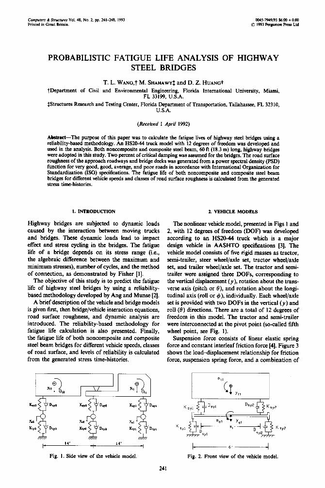
Fig. 3. The relationship between forces and displacements in the vehicle suspension system.

these two forces. The tire springs were assumed to be linear. In the suspension system, damping elements were assumed to be linear and viscous. Damping force is proportional to velocity. Ten percent of critical damping value was used for the damping coefficient [5]. Damping forces in the tires were neglected. Provision was made in the model for wheel lift; under this condition, the vertical tire stiffness was taken as zero.

The total potential energy, V = C Vi, of the system is computed from the spring stiffnesses and relative displacements, whereas the dissipation energy, D = I;Di, of the system is obtained from the damping forces. The total kinetic energy, T = ET, of the system is calculated using the mass, mass moment of inertia, and translational as well as rotational

velocities, of the system components. The moment of inertia of all components is assumed to be constant with the weight of each component acting as the external force on that component.

The equations of motion of the system are derived, using Lagrange’s formulation, as follows:

(1)

which q, and di are the generalized displacements and velocities. Details of derivation are presented in [6].

3. BRIDGE MODEL

According to AASHTO specifications [3] and [7j, both noncomposite and composite steel beam, 60ft

I- f KWx230 for Noncompoaite Beam Bridge WSs(lxl94 for Componite Beam Bridge

-I

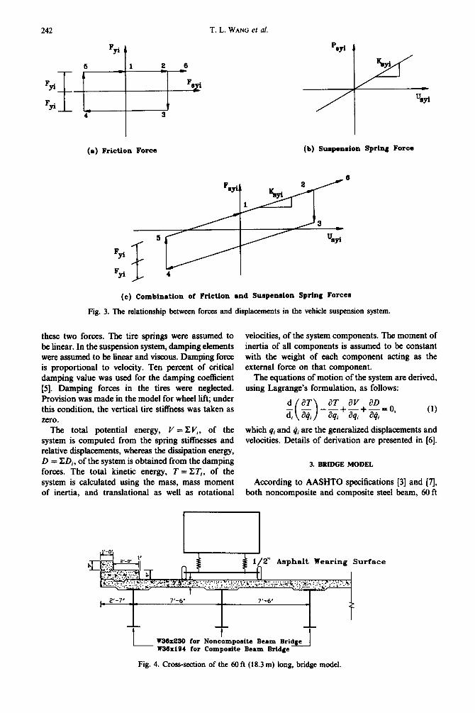
Fig. 4. Cross-section of the 60 fi (18.3 m) long, bridge model.

Fatigue life of highway steel bridges 243

Transformed

Effective Width

0.108 x 90” = 9.72”

7 1” haunch

W 36 x 194

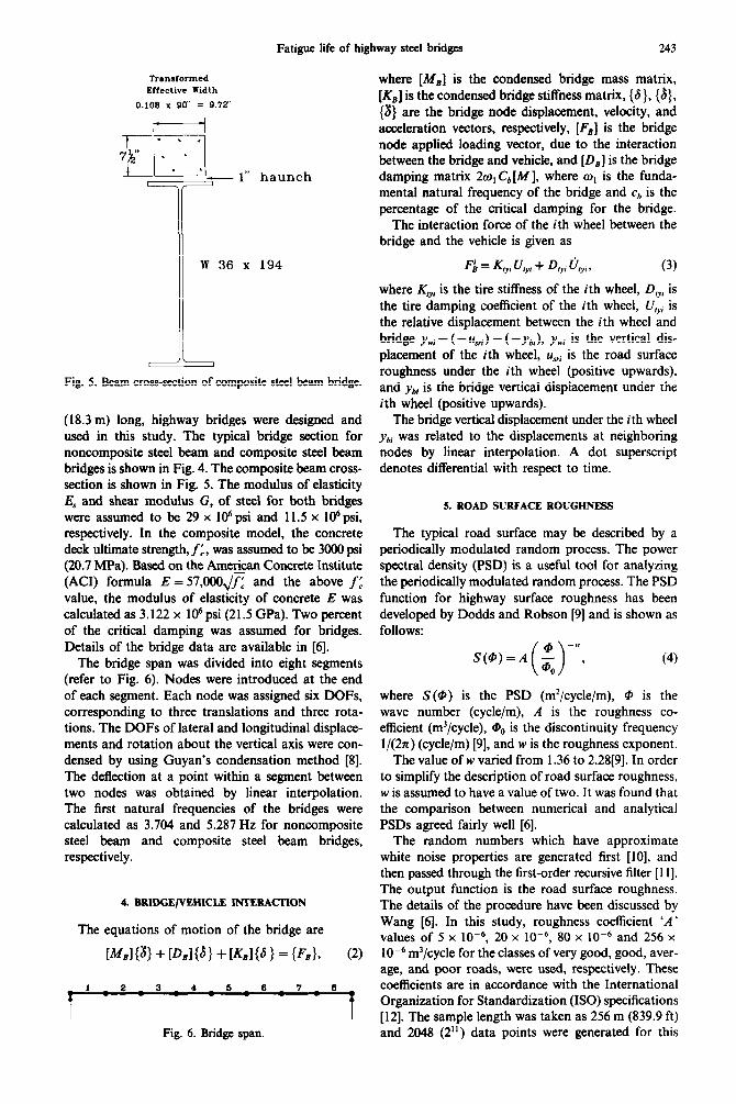
Fig. 5. Beam cross-section of composite steel beam bridge.

(18.3 m) long, highway bridges were designed and used in this study. The typical bridge section for noncomposite steel beam and composite steel beam bridges is shown in Fig. 4. The composite beam cross- section is shown in Fig. 5. The modulus of elasticity E, and shear modulus G, of steel for both bridges were assumed to be 29 x 106psi and 11.5 x 106psi, respectively. In the composite model, the concrete deck ultimate strength, f f , was assumed to be 3000 psi (20.7 MPa). Based on the American Concrete Institute (ACI) formula E = 57,000,,/ and the above f: value, the modulus of elasticity of concrete E was calculated as 3.122 x 106 psi (21.5 GPa). Two percent of the critical damping was assumed for bridges. Details of the bridge data are available in [6].

The bridge span was divided into eight segments (refer to Fig. 6). Nodes were introduced at the end of each segment. Each node was assigned six DGFs, corresponding to three translations and three rota- tions. The DOFs of lateral and longitudinal displacements and rotation about the vertical axis were condensed by using Guyan’s condensation method [8]. The deflection at a point within a segment between two nodes was obtained by linear interpolation. The first natural frequencies of the bridges were calculated as 3.704 and 5.287 Hz for noncomposite steel beam and composite steel beam bridges, respectively.

4. BRIDGE/VEHICLE INTERACTION

The equations of motion of the bridge are

MB1 @I + WBI @ I+ K?zl@ I = PC4 (2)

Fig. 6. Bridge span.

where [MB] is the condensed bridge mass matrix, [&] is the condensed bridge stiffness matrix, (a}, (61, {z} are the bridge node displacement, velocity, and acceleration vectors, respectively, [FJ is the bridge node applied loading vector, due to the interaction between the bridge and vehicle, and [DB] is the bridge damping matrix 2o,C,[A4], where o, is the funda- mental natural frequency of the bridge and cb is the percentage of the critical damping for the bridge.

The interaction force of the ith wheel between the bridge and the vehicle is given as

FL = Kyi u,i + D,yi o,yi 9 (3)

where K,yi is the tire stiffness of the ith wheel, D,yi is the tire damping coefficient of the ith wheel, U,Yi is the relative displacement between the ith wheel and bridge y, - (-a,.) - ( -ybi), ywi is the vertical displacement of the ith wheel, u,,~ is the road surface roughness under the ith wheel (positive upwards), and ybi is the bridge vertical displacement under the ith wheel (positive upwards).

The bridge vertical displacement under the ith wheel ybi was related to the displacements at neighboring nodes by linear interpolation. A dot superscript denotes differential with respect to time.

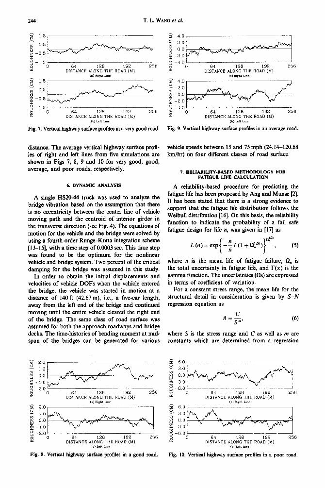
5. ROAD SURFACE ROUGHNESS

The typical road surface may be described by a periodically modulated random process. The power spectral density (PSD) is a useful tool for analyzing the periodically modulated random process. The PSD function for highway surface roughness has been developed by Dodds and Robson [9] and is shown as follows:

S(@)=A $ +, ( )’ 0 (4)

where S(Q) is the PSD (m2/cycle/m), @ is the wave number (cycle/m), A is the roughness coefficient (m3/cycle), 3 is the discontinuity frequency 1/(2x) (cycle/m) [9], and w is the roughness exponent.

The value of w varied from 1.36 to 2.28[9]. In order to simplify the description of road surface roughness, w is assumed to have a value of two. It was found that the comparison between numerical and analytical PSDs agreed fairly well (61.

The random numbers which have approximate white noise properties are generated first [lo], and then passed through the first-order recursive filter [l 11. The output function is the road surface roughness. The details of the procedure have been discussed by Wang [6]. In this study, roughness coefficient ‘A’ values of 5 x 10m6, 20 x 10m6, 80 x 10m6 and 256 x 10m6 m3/cycle for the classes of very good, good, average, and poor roads, were used, respectively. These coefficients are in accordance with the International Organization for Standardization (ISO) specifications [12]. The sample length was taken as 256 m (839.9 ft) and 2048 (2”) data points were generated for this


256

Fig. 7. Vertical highway surface profiles in a very good road. Fig. 9. Vertical highway surface profiles in an average road.

distance. The average vertical highway surface profiles of right and left lines from five simulations are shown in Figs 7, 8, 9 and 10 for very good, good, average, and poor roads, respectively.

6. DYNAMIC ANALYSIS

A single HS20-44 truck was used to analyze the bridge vibration based on the assumption that there is no eccentricity between the center line of vehicle moving path and the centroid of interior girder in the transverse direction (see Fig. 4). The equations of motion for the vehicle and the bridge were solved by using a fourth-order Rung*Kutta integration scheme [13-151, with a time step of 0.0003 sec. This time step was found to be the optimum for the nonlinear vehicle and bridge system. Two percent of the critical damping for the bridge was assumed in this study.

In order to obtain the initial displacements and velocities of vehicle DOFs when the vehicle entered the bridge, the vehicle was started in motion at a distance of 140ft (42.67m), i.e., a five-car length, away from the left end of the bridge and continued moving until the entire vehicle cleared the right end of the bridge. The same class of road surface was assumed for both the approach roadways and bridge decks. The time-histories of bending moment at midspan of the bridges can be generated for various

s -2.0 1 2 0 tIrs6T4ANCEz ALOKhE Fzo.4b9&, 256

(b) Len !dnc

Fig. 8. Vertical highway surface profiles in a good road.

2 20

g 0.0 !iz z -2.0 4 -4.0 r> -1 0 ir

0 64 128 192 256 DISTANCE ALONG THE ROAD(M)

(a, Right Lme s 4.0

u 2.0

g 0.0

: -2 0

s-4oL-------------- J

& 0

DIS?ANCE ALOiJ?GBTHE ROAi)‘&) 256

vehicle speeds between 15 and 75 mph (24.14-120.68 km/hr) on four different classes of road surface.

7. RELIABILJIY-BASED METHODOLOGY FOR FATIGUE LIFE CALCULATION

A reliability-based procedure for predicting the fatigue life has been proposed by Ang and Munse [2]. It has been stated that there is a strong evidence to support that the fatigue life distribution follows the Weibull distribution [16]. On this basis, the reliability function to indicate the probability of a fail safe fatigue design for life n, was given in [ 17] as

L(n)=exp -:f(l+R:08) “*, i

(5) n 1

where ii is the mean life of fatigue failure, Q, is the total uncertainty in fatigue life, and I(x) is the gamma function. The uncertainties (as) are expressed in terms of coefficient of variation.

For a constant stress range, the mean life for the structural detail in consideration is given by S-N regression equation as

C A=--,

S”

where S is the stress range and C as well as m are constants which are determined from a regression

DIs6T"ANCE ALOi&HE ROAf&) 256

(a, Right l.tne s 60

= 30

w bz

00

5 -30

>-60 zi 0 Dd?ANCE ALOi%?THE ROAbg:M, 256

Fig. 10. Vertical highway surface profiles in a poor road.

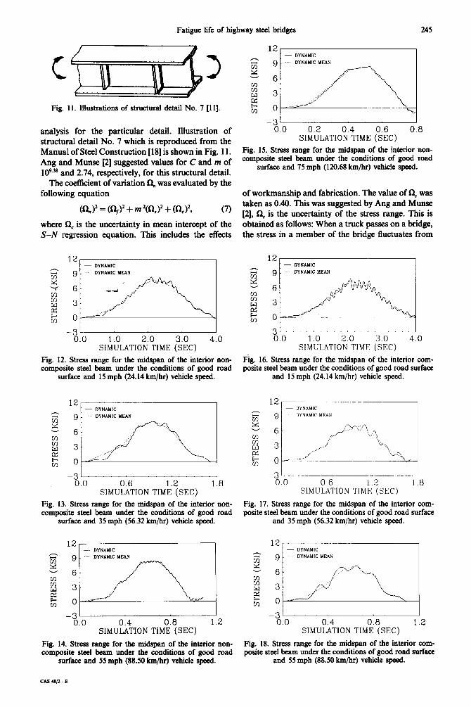
Fig. 11. Illustrations of structural detail No. 7 [1 I].

analysis for the particular detail. Illustration of 0.0 0.2 0.4 0.6 0.8

structural detail No. 7 which is reproduced from the SIMULATION TIME (SEC)

Manual of Steel Construction [ 181 is shown in Fig. 11. Fig. 15. Stress range for the midspan of the interior non-

Ang and Munse [2] suggested values for C and m of composite steel beam under the conditions of good road

1Og.3* and 2.74, respectively, for this structural detail. surface and 75 mph (120.68 km/hr) vehicle speed.

The coefficient of variation a, was evaluated by the

following equation of workmanship and fabrication. The value of Q was

(Qn 1’ = (f&Y + m W, )* + (Cl,)*, (7) taken as 0.40. This was suggested by Ang and Munse [2], Q is the uncertainty of the stress range. This is

where a, is the uncertainty in mean intercept of the obtained as follows: When a truck passes on a bridge, S-N regression equation. This includes the effects the stress in a member of the bridge fluctuates from

12 12 - DYNAMlC - DYNAMlC

- g DYNAMK MEAN - 9 z DYNAWCMEAN

-3’ I -3’ 0.0 1.0 2.0 3.0 4.0 0.0 1.0 2.0 3.0 4.0

SIMULATION TIME (SEC) SIMULATION TIME (SEC)

Fig. 12. Stress range for the midspan of the interior non- Fig. 16. Stress range for the midspan of the interior com- composite steel beam under the conditions of good road posite steel beam under the conditions of good road surface

surface and 15 mph (24.14 km/hr) vehicle speed. and 15 mph (24.14 km/hr) vehicle speed.

12 - DYNAMIC

- 9 DYNAMICYEAN z - 6

g 3-

cn 0

-3’ I _ 3 L_________i __ -._..-. ! 0.0 0.6 1.2 1.8 0.0 0.6 I.‘> I.8

SIMULATION TIME (SEC) SIMULATION TIMI;: (SEC)



12 - DYNAMK

- 9 i7; DYNAMK MEAN

-3U--.- -3' I 0.0 0.4 0.8 1.2 0.0 0.4 0.8 1.2

SIMULATION TIME (SEC) SIMULATION TIME (SEC)



Fatigue life of highway steel bridges

12, - DYNAYK

T. L. WANG et al.

-3t 0.0 0.2 0.4 0.6 0.8

SIMULATION TIME (SEC)

Fig. 19. Stress range for the midspan of the interior composite steel beam under the conditions of good road surface

and 75 mph (120.68 km/hr) vehicle speed.

a normal pattern. By averaging the values as many times as necessary, the fluctuations can be smoothed. The standard deviation computed from the deviations of the smoothed curve is divided by the arithmetic mean of all the stress points and is taken as R,.

Typical curves for computing stress ranges and R, are shown in Figs 12-19, f$ is the uncertainty of fatigue life data and model. It is shown as follows:

a, = ./<+>’ + (A,,,‘, (8

where Af is the uncertainty of the fatigue model used in the analysis. This includes errors introduced by the Miner’s [ 191 damage rule and the effects of mean stress in the S-N relationship. The value of A, was taken as 0.15, as suggested by Ang and Munsc [2], 8, is the average scatter of the fatigue life data about the S-N regression line. The values of 8, were taken as 0.49 for detail No. 7. These were suggested by Ang and Munse [2].

a RESULTS OF FATIGUE LIFE PREDICI’ION

The following assumptions were made in estimating the fatigue life of both bridges:

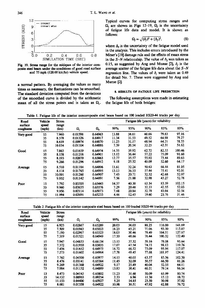
Table 1. Fatigue life of the interior noncomposite steel beam based on 100 loaded HS20-44 trucks per day

Road Vehicle stress Fatigue life (years) for reliability surface range -

fOUgh!ESS tzi OtSQ 9 f-A 99% 95% 90% 85% 80%

- Very good 15 7.960 0.01598 0.64963 13.88 38.61 60.66 79.63 97.16 35 8.578 0.01326 0.64917 11.34 31.53 49.52 64.98 79.27 55 8.618 0.00974 0.64870 11.23 31.17 48.94 64.21 78.33 75 10.034 0.01104 0.64886 7.39 20.54 32.25 42.31 51.62

Good 15 7.863 0.01659 0.64974 14.35 39.92 62.72 82.33 100.46 35 8.138 0.01218 0.64901 13.12 36.44 57.22 75.09 91.60 55 8.193 0.02070 0.65063 12.77 35.57 55.92 73.44 89.63 75 9.266 0.012% 0.64912 9.18 25.52 40.09 52.60 64.17

Average 15 8.510 0.01184 0.64896 11.61 32.24 50.63 66.44 81.05 35 8.118 0.01765 0.64995 13.13 36.55 57.44 75.41 92.01 55 10.001 0.01260 0.64907 7.45 20.71 32.52 42.68 52.07 75 9.952 0.01142 0.64891 7.56 21.09 32.98 43.27 52.78

Poor :: 7.792 0.03305 0.65445 14.37 40.30 63.54 83.59 102.15 9.960 0.03635 0.65576 7.29 20.48 32.33 42.55 52.03

55 9.956 0.02114 0.65073 7.48 20.84 32.78 43.04 52.54 75 11.994 0.02691 0.65233 4.46 12.45 19.60 25.76 31.46

Table 2. Fatigue life of the interior composite steel beam based on 100 loaded HS20-44 trucks per day

Road Vehicle Stress Fatigue life (years) for reliability SurfaCe range

rOUghlESS Et 04 4 4 99% 95% 90% 85% 80%

Very good 15 6.923 0.02867 0.65289 20.03 56.03 88.25 116.00 141.69 35 7.509 0.01943 0.65033 16.23 45.21 71.06 93.30 113.87 55 7.190 0.02967 0.65323 18.03 50.46 79.49 104.51 127.67 75 7.319 0.01521 0.64949 17.50 48.66 76.44 100.32 122.40

Good 15 7.947 0.04833 0.66154 13.15 37.32 59.16 78.08 95.64 35 7.372 0.01950 0.65035 17.07 47.54 74.73 98.13 119.76 55 7.436 0.01652 0.64973 16.72 46.52 73.09 95.94 117.07 75 7.273 0.01602 0.64964 17.78 49.45 77.68 101.97 124.41

Average 15 7.762 0.04500 0.65977 14.15 40.03 63.37 83.56 102.30 35 8.476 0.03141 0.65384 11.45 32.09 50.57 66.50 81.26 55 9.269 0.01360 0.64922 9.17 25.49 40.04 52.55 64.11 75 7.984 0.01132 0.64889 13.83 38.41 60.31 79.14 96.54

Poor :: 8.473 0.04143 0.65802 11.23 31.68 50.09 65.99 80.74 14.132 0.08903 0.69254 2.33 6.96 11.30 15.12 18.72

55 11.153 0.044cM 0.65927 5.25 14.85 23.50 30.98 37.92 75 8.681 0.01358 0.64922 10.98 30.51 47.92 62.88 76.72

Fatigue life of highway steel bridges 241

s 0 I I b 0’ I

L 10 20 30 40 50 60 70 80 iz 10 20 30 40 50 60 70 80 VEHICLE SPEED (MPH) VEHICLE SPEED (MPH)

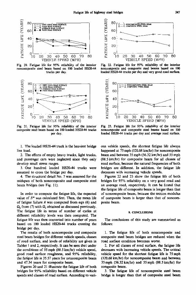
Fig. 20. Fatigue life for 95% reliability of the interior Fig. 22. Fatigue life for 95% reliability of the interior noncomposite steel beam based on 100 loaded HS20-44 noncomposite and composite steel beams based on 100

trucks per day. loaded HS20-44 trucks per day and very good road surface.

10 20 30 40 50 60 70 80 VEHICLE SPEED(MPH) VEHICLE SPEED (MPH)

Fig. 21. Fatigue life for 95% reliability of the interior Fig. 23. Fatigue life for 95% reliability of the interior composite steel beam based on 100 loaded HS20-44 trucks noncomposite and composite steel beams based on 100

per day. loaded HS20-44 trucks per day and average road surface.

1. The loaded HS20-44 truck is the heaviest bridge live load.

2. The effects of empty heavy trucks, light trucks, and passenger cars were neglected since they only develop small stress ranges.

3. One hundred loaded HS20-44 trucks were assumed to cross the bridge per day.

4. The structural detail No. 7 was assumed for the midspan of both noncomposite and composite steel beam bridges (see Fig. 11).

In order to compute the fatigue life, the expected value of S” was calculated first. Then, the mean life of fatigue failure fi was computed from eqn (6) and R, from (7) with C& obtained as discussed previously. The fatigue life in terms of number of cycles at different reliability levels was then computed. The fatigue life was then converted into number of years based on 100 loaded HS20-44 trucks crossing the bridge per day.

The results of both noncomposite and composite steel beam bridges for different vehicle speeds, classes of road surface, and levels of reliability are given in Tables 1 and 2, respectively. It can be seen that under the conditions of 55 mph (88.5 km/hr) vehicle speed, good road surface roughness, and 95% reliability, the fatigue life is 35.57 years for noncomposite beam and 47.54 years for composite beam.

Figures 20 and 21 illustrate the fatigue life of both bridges for 95% reliability based on different vehicle speeds and classes of road surface. According to vari-

ous vehicle speeds, the shortest fatigue life always happened at 75 mph (120.68 km/hr) for noncomposite beam and between 35 mph (56.32 km/hr) and 55 mph (88.5 km/hr) for composite beam for all classes of road surface, because the natural frequencies of both bridges are different. In addition, the fatigue life decreases with increasing vehicle speeds.

Figures 22 and 23 show the fatigue life of both bridges for 95% reliability on a very good road and an average road, respectively. It can be found that the fatigue life of composite beam is longer than that of noncomposite beam, because the section modulus of composite beam is larger than that of noncomposite beam.

9. CONCLUSIONS

The conclusions of this study are summarized as fo11ows:

1. The fatigue life of both noncomposite and composite steel beam bridges are reduced when the road surface condition becomes worse.

2. For all classes of road surface, the fatigue life decreases with increasing vehicle speeds. The critical vehicle speed for the shortest fatigue life is 75 mph (120.68 km/hr) for noncomposite beam and between 35 mph (56.32 km/hr) and 55 mph (88.5 km/hr) for composite beam.

3. The fatigue life of noncomposite steel beam bridge is longer than that of composite steel beam


bridge based on the same running conditions, except poor road surface roughness.

4. A reduced percentage of reliability results in longer fatigue life.

5. In classes of very good and good road surface, the range of fatigue life varied from 39.92 to 20.54 years for noncomposite steel beam bridge and from 56.03 to 37.32 years for composite steel beam bridge, based on the 95% reliability and vehicle speeds from 15 to 75 mph (24.14-120.68 km/hr).

REFERENCES

I. J. W. Fisher, Guide to 1974 AASHTO Fatigue Specifica- tions. American Institute of Steel Construction, New York (1977).

2. A. H.-S. Ang and W. H. Munse, Practical reliability basis for structural fatigue. AXE, National Structural Engineering Conference, Preprint 2492, April (1975).

3. Standard Specifications for Highway Bridges, 14th Edn. American Association of State Highway and Trans- portation Officials, Washington, D.C. (1989).

4. T. Huang, Dynamic response of three-span continuous highway bridges. Ph.D. dissertation, University of Illinois, Urbana, IL (1960).

5. A. P. Whittemore, J. R. Wiley, P. C. Schultz and D. E. Pollock, Dynamic pavement loads of heavy highway vehicles. National Cooperative Highway Research Program Report, Washington, D.C. (1970).

6. T. L. Wang, Computer modeling analysis in bridge evaluation. Final research report prepared for Florida Department of Transportation under contract No. C-3394 (WPI-0510542), Tallahassee, FL, in press.

7.

8.

9.

10.

11.

12.

13.

14.

15.

16.

17.

18.

19.

C. P. Heins and D. A. Firmage, Design of Modern Steel Highway Bridges. John Wiley, New York (1979). R. J. Guyan, Reduction of stiffness and mass matrices. Am. Insr. Aeronaut. Astronaut. Jnl3, 380 (1965). C. J. Dodds and J. D. Robson, The description of road surface roughness. J. Sound Vibr. 31, 175-183 (1973). J. Moshman, Random number generation. In Marhe- matical Methods for Digital Computers (Edited by A. Ralston and H. S. Will), Vol. II, Chap. 12, pp. 249-263. John Wiley, New York (1967). R. K. Otnes and L. Enochson, Digital Time Series Analysis. John Wiley, New York (1972). C. J. Dodds, BSI Proposals for Generalized Terrain Dynamic Inputs to Vehicles. ISO/TC/lOS/WG9, Docu- ment No. 5, International Organization for Standardiz- ation (1972). K. H. Chu, V. K. Garg and T. L. Wang, Impact in railway prestressed concrete bridges. J. Struct. Engng, ASCE 112, 1036-1051 (1986). T. L. Wang, Ramp/bridge interface in railway prestressed concrete bridges. J. Struct. Engng, ASCE 116, 1648-1659 (1990). T. L. Wang, V. K. Garg and K. H. Chu, Railway bridge/vehicle interaction studies with a new vehicle model. J. Struck Engng, ASCE 117, 2099-2116 (1991). A. M. Freudenthal, Prediction of fatigue failure. J. appl. Phys. 31, 2196-2198 (1960). A. H.-S. Ang, A comprehensive basis for reliability analysis and design. Proc. of U.S.-Japan Joint Seminar on Reliability Approach in Structural Engineering, Tokyo, Japan, May (1974). Manual of Steel Construction, 9th Edn. American Institute of Steel Construction, Chicago, IL (1989). M. A. Miner, Cumulative damage in fatigue. J. appl. Mech., ASME 12, A159-A164 (1945).

Documents

Probabilistic fatigue life analysis of highway steel bridges