Embed Size (px)
Citation preview
PROBABILISTIC ASSET VALUATION APPLIED TO NATURAL RESOURCE PROJECTS
by
Michal Wypych B.ASc, University of British Columbia 2005
PROJECT SUBMITTED IN PARTIAL FULFILLMENT OF THE REQUIREMENTS FOR THE DEGREE OF
MASTER OF BUSINESS ADMINISTRATION
In the Executive Master of Business Administration Program of the
Faculty of
Business Administration
© Michal Wypych 2011
SIMON FRASER UNIVERSITY
Spring 2011
All rights reserved. However, in accordance with the Copyright Act of Canada, this work may be reproduced, without authorization, under the conditions for Fair Dealing.
Therefore, limited reproduction of this work for the purposes of private study, research, criticism, review and news reporting is likely to be in accordance with the law,
particularly if cited appropriately.
brought to you by COREView metadata, citation and similar papers at core.ac.uk
provided by Simon Fraser University Institutional Repository
ii
Approval
Name: Michal Wypych
Degree: Executive Master of Business Administration
Title of Project: Probabilistic Asset Valuation Applied To Natural Resource Projects
Supervisory Committee:
___________________________________________
Scott Powell Senior Supervisor Adjunct Professor
___________________________________________
Dr. Ian P. McCarthy Second Reader Professor & Canada Research Chair in Technology & Operations Management
Date Approved: ___________________________________________
iii
Abstract
This paper develops three probabilistic asset valuation models for mining projects.
Firstly, an overview of available asset valuation techniques is presented. The probabilistic asset
valuation technique is described in greater detail in advance of developing the probabilistic
financial models. The probabilistic models incorporate a stochastic behaviour model for the price
of copper and a Chilean peso exchange rate correlated to the copper price. The stochastic model
parameters are defined based on the deterministic sensitivity analysis and on academic research.
A sensitivity analysis tests the influence of one parameter for which guidance from the
deterministic valuation process is not available. Three potential copper projects are evaluated
deterministically and probabilistically and outputs from each approach are compared.
Applications of the probabilistic approach are discussed along with implications on the decision
making process. Finally, a high level implementation strategy is presented aimed at overcoming
barriers for adopting probabilistic asset valuation.
iv
Executive Summary
Risk and reward typically move in tandem; higher risks demand higher reward. The
nature of natural resource projects is that the stakes of this trade-off are high. These projects
require large amounts of capital to develop. However, the profitability of these projects will be
dictated by future operating conditions. Commodity prices clearly have the greatest impact on
profitability. The most commonly used asset valuation methodology, deterministic discounted
cash flows, incorporates static commodity price assumptions. Risk due to commodity price
fluctuations is evaluated through sensitivity analysis. A limitation of this approach is that it
considers the impact of variables in isolation by varying them in fixed intervals. Probabilistic
asset valuation offers a different approach to evaluating risk. Defining variables such as
commodity prices stochastically in the financial model incorporates the random element inherent
in their long-term behaviour. In combination with Monte Carlo simulation, this methodology
examines a large number of commodity price profiles over the asset life and captures the effects
on financial metrics. Furthermore, correlations among variables can be defined in order to better
model real life economic conditions. The result of the simulation is a probability distribution of
selected financial metrics. This probability distribution quantifies risks associated with the
project. For example, the probability that a project generates a positive net present value (NPV) is
available to decision makers. In contrast, a deterministic sensitivity analysis is only able to show
the financial performance under a limited range of variable assumptions and rank the relative
impact among variables. This paper demonstrates the value added to project evaluation through
the application of probabilistic asset valuation. The NPVs of three projects are shown to be
potentially overstated based on deterministic financial models. Although lower, NPVs derived
from probabilistic models were still attractive. As a result, probabilistic asset valuation would
yield greater value added when applied to marginal projects, or under less favourable economic
conditions, than those considered in this report. This paper concludes that probabilistic asset
valuation has good potential to complement the deterministic valuation technique by improving
the current methodology for sensitivity analysis. The improved sensitivity analysis provides
decision makers with a tool for risk management of individual projects or among alternatives
when considering the dilemma of risk and financial reward.

v
Dedication
I would like to dedicate this report to Robin Fowler. Her influence originally set in
motion the events leading to the completion of this report and without her support, the journey
would not have been completed. Kocham Cię.
vi
Acknowledgements
I would like to extend a special thank you to Scott Powell and Dale Andres for their
guidance in completing this report. Scott’s extensive knowledge on the subject matter
significantly assisted the learning process and added to the outcomes of the report. Dale’s
industry experience helped to shape the original direction of the project. In addition, thank you to
members of Teck’s executives who participated in the survey undertaken for this report. Their
input helped generate a strategy to incorporate the concepts evaluated in this report. Ongoing
support and assistance from Jason Sangha and Grant Piwek is very much appreciated.
vii
Table of Contents
Approval .......................................................................................................................................... iiAbstract .......................................................................................................................................... iiiExecutive Summary ........................................................................................................................ ivDedication ........................................................................................................................................ vAcknowledgements ......................................................................................................................... viTable of Contents .......................................................................................................................... viiList of Figures .............................................................................................................................. viiiList of Tables ................................................................................................................................... ix
1.0 Introduction ........................................................................................................................... 1
2.0 Asset Valuation Techniques ................................................................................................. 2
3.0 Deterministic Asset Valuation .............................................................................................. 8
4.0 Probabilistic Asset Valuation ............................................................................................. 19
5.0 Application ........................................................................................................................... 39
6.0 Implementation .................................................................................................................... 41
7.0 Conclusion ............................................................................................................................ 44
Appendices .................................................................................................................................... 46Appendix A .................................................................................................................................... 47Appendix B ..................................................................................................................................... 48Appendix C ..................................................................................................................................... 49Appendix D .................................................................................................................................... 50Appendix E ..................................................................................................................................... 51Appendix F ..................................................................................................................................... 52Appendix G .................................................................................................................................... 53
Reference List ............................................................................................................................... 56
viii
List of Figures
Figure 1. Banff Taxonomy ............................................................................................................... 2
Figure 2. Percent of CFOs who always or almost always use a given technique ............................. 4
Figure 3. Project A NPV sensitivity analysis ................................................................................. 11
Figure 4. Project B NPV sensitivity analysis ................................................................................. 14
Figure 5. Project C NPV sensitivity analysis ................................................................................. 16
Figure 6. One iteration of stochastic models applied to the price of copper .................................. 20
Figure 7. A second iteration of stochastic models applied to the price of copper .......................... 21
Figure 8. One iteration with constrained Random Walk models .................................................... 23
Figure 9. Copper Price and Chilean Peso exchange rate data since 2002 ...................................... 25
Figure 10. Project A NPV histogram ............................................................................................. 26
Figure 11. Project A IRR histogram ............................................................................................... 27
Figure 12. Project A payback period histogram ............................................................................. 28
Figure 13. Project B NPV histogram .............................................................................................. 30
Figure 14. Project B IRR histogram ............................................................................................... 31
Figure 15. Project B payback period histogram ............................................................................. 31
Figure 16. Project C NPV histogram .............................................................................................. 33
Figure 17. Project C IRR histogram ............................................................................................... 34
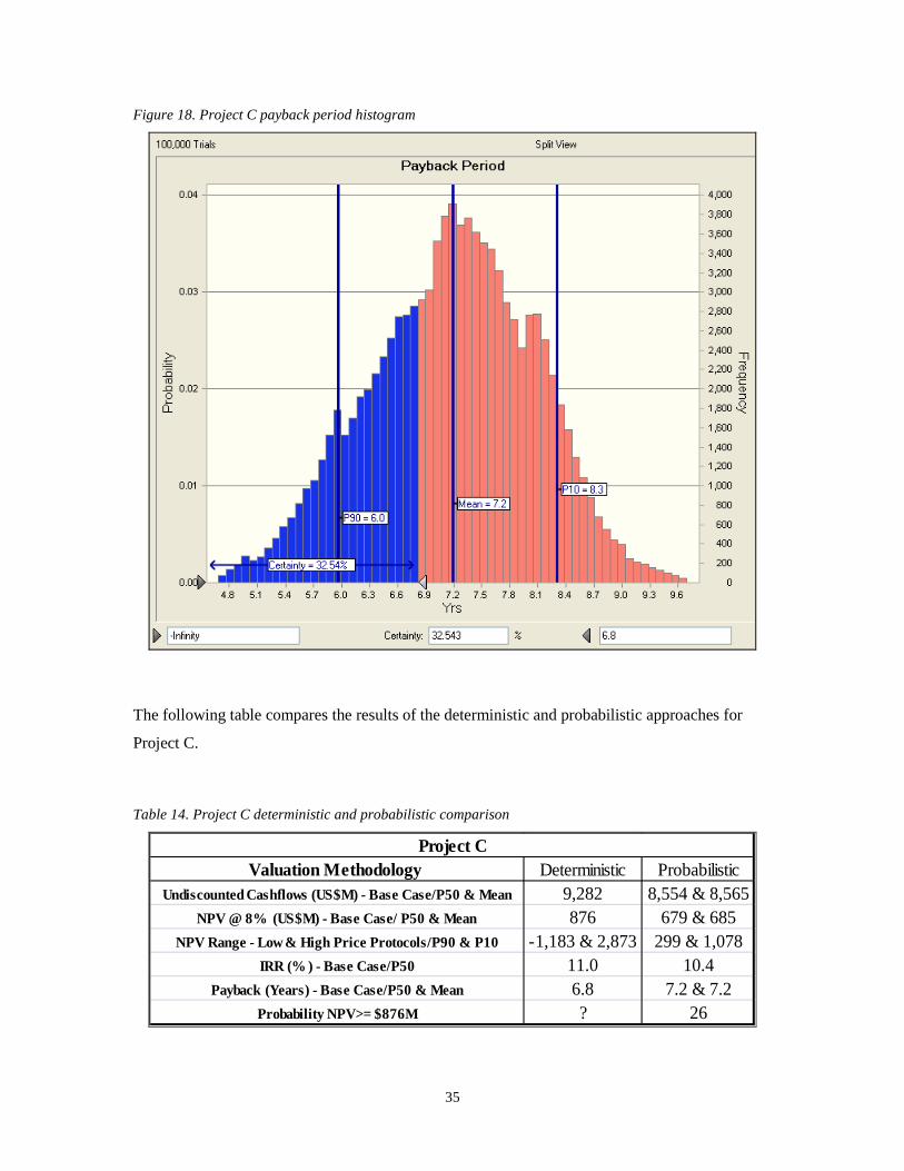
Figure 18. Project C payback period histogram ............................................................................. 35
Figure 19. Teck responses to probabilistic asset valuation survey ................................................. 42
ix
List of Tables
Table 1. Project A assumptions ........................................................................................................ 9
Table 2. Financial performance of Project A ................................................................................... 9
Table 3. Range of input variables for sensitivity analysis .............................................................. 10
Table 4. Range of possible model outputs from sensitivity analysis for Project A ........................ 11
Table 5. Project B assumptions ...................................................................................................... 12
Table 6. Financial performance of Project B .................................................................................. 13
Table 7. Range of possible model outputs from sensitivity analysis for Project B ........................ 14
Table 8. Project C assumptions ...................................................................................................... 15
Table 9. Financial performance of Project C .................................................................................. 15
Table 10. Range of possible model outputs from sensitivity analysis for Project C ...................... 16
Table 11 Deterministic Project Comparison .................................................................................. 17
Table 12. Project A deterministic and probabilistic comparison .................................................... 28
Table 13. Project B deterministic and probabilistic comparison .................................................... 32
Table 14. Project C deterministic and probabilistic comparison .................................................... 35
Table 15. Probabilistic model sensitivity to reversion parameter ................................................... 37
1
1.0 Introduction
At Teck, large scale mining projects are evaluated on the merits of safety, environmental
and social sustainability, and profitability, among others. Gauging the profitability of a project is
an integral part of the evaluation process. A wide range of variables can influence profitability.
Unknown variables are quantified with assumptions based on research, internal expertise, and
historical trends and compiled into financial models to provide an estimate of profitability.
Current financial modelling utilizes a deterministic methodology. With this approach, a static set
of assumptions produces a fixed output. This output for financial models includes indicators such
as NPV, rates of return, and payback period. Furthermore, sensitivity analysis is performed to
evaluate the effects of changes to the initial assumptions on a model’s outputs. However, the
current methodology fails to capture the uncertainty inherent in predicting variables outside the
company’s control and the uncertainty from basing assumptions on limited information. An
example of such a variable might include metal prices which cannot be forecast with certainty.
Therefore, as an alternative to the deterministic model, this paper will examine a probabilistic
approach to financial modelling for project evaluation. The probabilistic approach incorporates
the uncertainty of input assumptions, and returns a range of outputs. The use of a probabilistic
financial model will allow Teck to more accurately quantify and manage the inherent risk
associated with its development projects. Projects with lower risk profiles and a higher likelihood
of profitability can be identified and advanced to the next stage of development. Conversely,
projects less likely to be profitable can be studied further to reduce, if possible, the uncertainty of
underlying risks and assumptions.
2
2.0 Asset Valuation Techniques
Investment decisions depend heavily on the ability of management to value assets
correctly. The scale of the investment dictates the rigor of analysis applied to potential
investments. Long life and capital intensive projects in the mining industry require decision
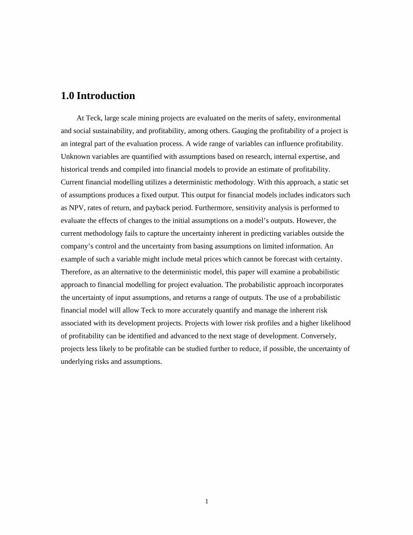
makers to utilize as many tools as possible to judge projects’ value. Laughton summarizes a
taxonomy of valuation methods known as the Banff Taxonomy1
Figure 1. Banff Taxonomy
. The Banff Taxonomy groups
valuation methods on a multidimensional spectrum of modelling and valuing uncertainty.
Of the valuation methods found in the preceding table, discounted cash flows (DCF), decision
trees, and real options account for the majority of methods employed for asset valuation, and
therefore warrant a closer review.
1 Laughton, 2007, p. 2
3
The DCF technique is the original valuation methodology and has been in practice for
over 50 years. In these models, forecasted future cash flows are discounted using a discount rate
reflecting the time value of money and a premium for the uncertainty of future cash flows. 1-
point DCF forecasts include single long term variable assumptions and produce a single output.
In conjunction with the 1-point analysis, firms often use DCF simple scenarios and simulation as
a form of sensitivity analysis. Simple scenarios include testing different variable assumptions
individually to determine the effects on the model’s output. On the other hand, DCF simulation
utilizes Monte Carlo simulation to run many different iterations of variable assumptions based on
a stochastic distribution. The results of the simulation produce confidence levels of the expected
model outputs. Decision tree analysis involves mapping all possible events and corresponding
responses available to management, in sequential order. The result is a branched roadmap with
many alternative paths forward. Each decision point represents a junction point in the path with
corresponding expected values and probabilities of each alternative. To ascertain the value of an
asset, management considers the likelihood of occurrence for each path and selects the highest
value path to match their risk profile. As a result, this technique captures the implications of
future decisions. Finally real options analysis takes the view that management is active, rather
than passive, and can modify project decisions in the future. The DCF methodology assumes that
management are passive and as a result the discount factor is used to account for possible
uncertainty of future cash flows. On the other hand, real options analysis assumes that future cash
flows are less uncertain because management is actively managing these cash flows and
accounting for risk in their decisions. As a result, the theory is that these cash flows should be
discounted at the risk free rate to reflect the lower level of uncertainty.
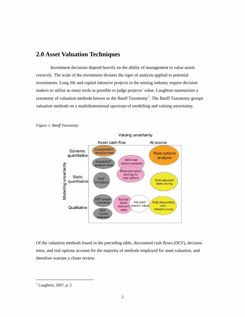
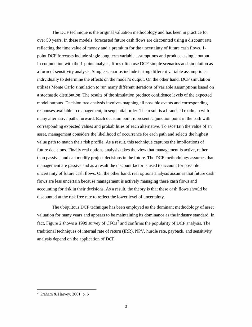
The ubiquitous DCF technique has been employed as the dominant methodology of asset
valuation for many years and appears to be maintaining its dominance as the industry standard. In
fact, Figure 2 shows a 1999 survey of CFOs2
and confirms the popularity of DCF analysis. The
traditional techniques of internal rate of return (IRR), NPV, hurdle rate, payback, and sensitivity
analysis depend on the application of DCF.
2 Graham & Harvey, 2001, p. 6
4
Figure 2. Percent of CFOs who always or almost always use a given technique
Figure 2 also highlights that evaluation techniques are not used in isolation. In most instances,
techniques such as NPV and sensitivity analysis are performed in tandem during asset valuation.
Other evaluation techniques are used by less than half of the surveyed CFOs. One reason might
be the unfamiliarity with more advanced techniques. In addition, the lack of consensus among the
academic community on fundamental aspects of these techniques, such as stochastic behaviour,
adds to the reluctance to accept other valuation methods beyond DCF.
Based on the usage statistics, it will take a significant effort to gain wide spread
acceptance of valuation techniques other than the traditional DCF. It should be made clear that
the use of the remaining valuation methods does not preclude management from using DCF.
Instead, DCF analysis can be supplemented with the more advanced methods to gain greater
insight regarding uncertainty. Slow rates of adoption are to be expected. The status quo has been
in practice for so many years that it has become engrained in many organizations. Moving beyond
industry standards will require a cultural shift for many managers. Incremental steps will be
required to achieve this cultural shift. The Banff Taxonomy and usage statistics show
probabilistic analysis as the next level of analysis beyond the comfortable DCF. Ho and Pike
addressed the adoption issues of probabilistic risk analysis (PRA). They surveyed firms in an
attempt to answer the following question: Does the adoption of PRA lead to a shift in a firm’s
5
capital investment? Literature on the answer to this question appears to be divided. Hull3 and
Hertz4 argue that PRA encourages investment. Since PRA can be used as a supplemental tool to
gauge uncertainty, it adds to the overall data set used for decision making. Ho and Pike
summarize this viewpoint as “PRA provides additional insights which may reduce descriptive and
managerial uncertainty, providing managers with incentives to increase investment”5. On the
other hand, Neuhauser and Viscione point out that some managers favour experience and
judgment over quantitative methods6. These managers feel that an overreliance on quantitative
models could overshadow the art of discerning a good investment from a poor one. As a result,
these managers may not support projects justified on the basis of a probabilistic analysis. In the
end, Ho and Pike’s empirical research concluded that the use of PRA techniques did not have a
negative impact on capital expenditures7. Subjectivity appears to be another hurdle for PRA
adoption. Bier mentions that practitioners of PRA can steer the analysis in different directions
based on differing goals and subjective judgment8. Furthermore, she adds that the implications of
subjectivity in a probabilistic model’s inputs are not fully appreciated9. Bier concludes that
further research on the application of PRA would benefit adoption efforts of this methodology10
The use of a stochastic process in financial models affords the user a wide range of
options. The absence of an industry standard in the use of stochastic models leads to variations in
application and illustrates the subjectivity concerns discussed earlier. Ideally, inputs are modelled
to represent the expected future behaviour. However, in most instances this is next to impossible.
For some inputs, historical data can provide the evidence necessary to select an appropriate
probability distribution. However, other variables, such as commodity prices, are less amenable to
predicting future behaviour on the basis of the past. For these variables, many predictive
behaviour models have been developed by the academic community. Two prominent behaviour
.
Ultimately, managers might require subject matter experts, internal or external, for guidance in
the use of more sophisticated valuation techniques. This guidance might prove beneficial in the
early stages of transitioning away from purely DCF valuation mindset, until a critical mass of
industry use is achieved.
3 Hull, 1980 4 Hertz, 1964, p. 95-106 5 Ho & Pike, 1992, p. 390 6 Neuhauser & Viscione, 1973, p. 21 7 Ho & Pike, 1992, p. 399 8 Bier, 1999, p. 705 9 Ibid. 10 Bier, 1999, p. 706
6
models for commodity prices include the Random Walk and Mean Reverting. One example of a
Random Walk model for commodity prices is based on geometric Brownian motion and takes the
following form:
Where: S = commodity price at time t
t = length of time between forecasting periods
change in commodity price between forecasting periods
α = short-term price growth rate
σ = short-term price volatility
dz = standard Weiner increment =
ε = standard normal random variable with a mean of 0 and standard variation of 1
The Random Walk model assumes a trend for the variable being modelled, captured by the first
part of the equation. If the short-term growth rate is zero, this model is referred to as a pure
Random Walk model. Otherwise, the model is referred to as Random Walk with drift. The second
part of the equation represents the Random Walk aspect. In this part, shocks are applied to the
change in value of the variable based on a standard normal random variable. This model could be
applied where there is consensus among management that the commodity in question will exhibit
a constant trending behaviour. Dixit and Pindyck point out that the past behaviour of
commodities resembles Random Walk characteristics when evaluating data for the previous 30 or
40 years. However, when the time horizon is expanded beyond 100 years, the Random Walk
hypothesis can be rejected in favour of a Mean Reverting process11. One model is based on the
Ornstein-Uhlenbeck process12
11 Dixit & Pindyck, 1994, p. 77-78
which defines a Mean Reverting stochastic process with
applications in modelling interest rates, exchange rates, and commodity prices. This Mean
Reverting model takes the following form:
12 Ornstein & Uhlenbeck, 1930, p. 823
7
Where: S = commodity price at time t
t = length of time between forecasting periods
change in commodity price between forecasting periods
Sm = long-term equilibrium commodity price
γ = reversion rate
σ = short-term price volatility
dz = standard Weiner increment =
ε = standard normal random variable with a mean of 0 and standard variation of 1
The second part of this model includes the same random shock aspects as the previous Random
Walk model. The difference is in the first part of the equation, where the variable being modelled
is always pulled towards an equilibrium value. Application of the Mean Reverting model is
appropriate where management has a long term view of a commodity but wishes to include the
unpredictable nature of future commodity prices. In a study of 300 commodities, Andersson
supports the mean-reverting nature of commodities. He asserts that high prices attract new
entrants thereby increasing supply and reverting prices towards the marginal cost of production13.
Further support of the Mean Reverting process in modelling future commodity price behaviour is
provided by Bernard, et al.14 and Schwartz15
.
13 Andersson, 2007, p. 781 14 Bernard, Khalaf, Kichian, & Mcmahon, 2008, p. 289 15 Schwartz, 1997, p. 926
8
3.0 Deterministic Asset Valuation
A deterministic financial model incorporates a fixed set of assumptions to produce fixed
outputs. These models incorporate the DCF methodology. The current practice of asset valuation
at Teck is based on deterministic models to produce metrics such as NPV, IRR, and payback
period in addition to performing 1-point sensitivity analysis. In this section, three projects are
presented along with deterministic DCF valuation metrics. The deterministic financial models of
all three projects are Microsoft Excel based and project revenues, costs, free cash flows, and
discounted cash flows. To protect corporate confidentiality, the projects are named A, B, and C.
The results of this analysis will serve as a base case for comparison of a valuation process using a
probabilistic financial model.
Project A is a potential copper and gold open pit mine located in Chile. Engineering
studies have identified a 19 year mine life along with a production schedule. The mine will
produce one concentrate, containing copper and gold, which will be sold to smelters. The
deterministic financial model will project annual cash inflows based on fixed variable inputs and
subtract annual outflows such as operating costs, initial and sustaining capital, and taxes. The net
annual cash flows will be discounted from the year they occur and totalled to determine the NPV.
In addition, the IRR and payback period will be presented. IRR is calculated as the rate of return
required to achieve an NPV of zero. The payback period is the number of years required to
recover initial capital costs, based on undiscounted cash flows. Project A is analyzed in first
quarter 2011 US dollars, with no allowance for inflation, on the basis of 100% equity financing.
A summary of the financial model is included in Appendix A.
9
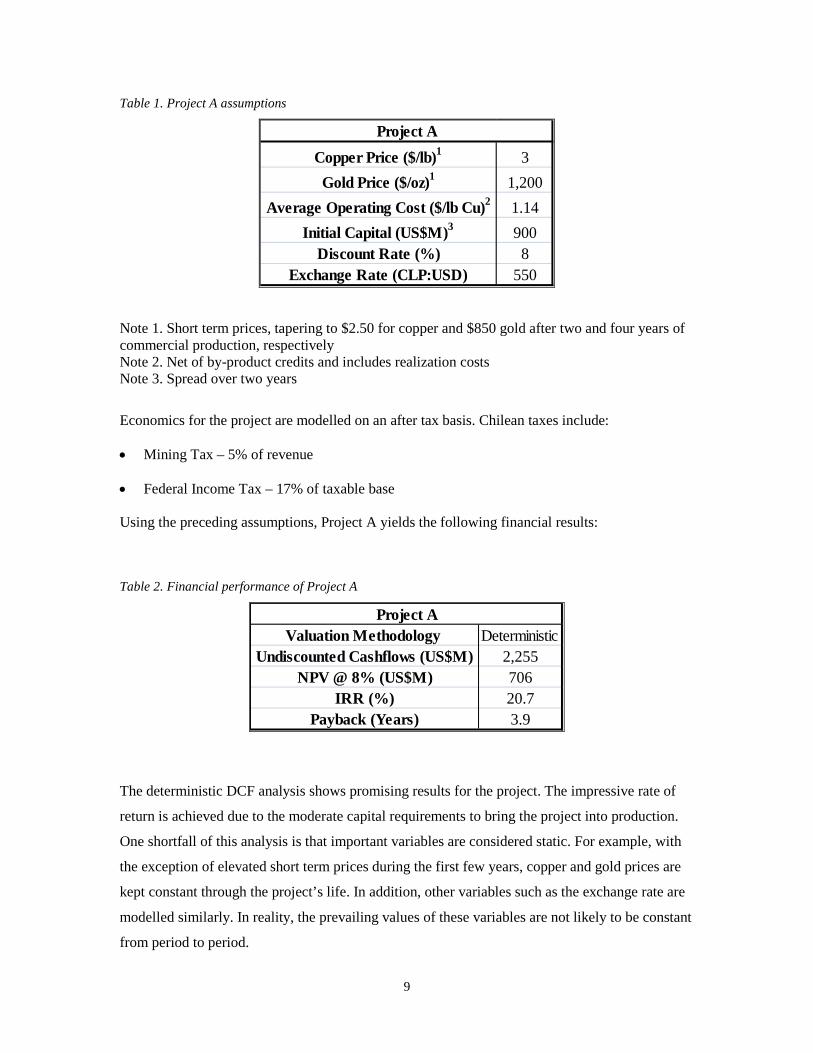
Table 1. Project A assumptions
Copper Price ($/lb)1 3Gold Price ($/oz)1 1,200
Average Operating Cost ($/lb Cu)2 1.14Initial Capital (US$M)3 900
Discount Rate (%) 8Exchange Rate (CLP:USD) 550
Project A
Note 1. Short term prices, tapering to $2.50 for copper and $850 gold after two and four years of commercial production, respectively Note 2. Net of by-product credits and includes realization costs Note 3. Spread over two years
Economics for the project are modelled on an after tax basis. Chilean taxes include:
• Mining Tax – 5% of revenue
• Federal Income Tax – 17% of taxable base
Using the preceding assumptions, Project A yields the following financial results:
Table 2. Financial performance of Project A
Valuation Methodology DeterministicUndiscounted Cashflows (US$M) 2,255
NPV @ 8% (US$M) 706IRR (%) 20.7
Payback (Years) 3.9
Project A
The deterministic DCF analysis shows promising results for the project. The impressive rate of
return is achieved due to the moderate capital requirements to bring the project into production.
One shortfall of this analysis is that important variables are considered static. For example, with
the exception of elevated short term prices during the first few years, copper and gold prices are
kept constant through the project’s life. In addition, other variables such as the exchange rate are
modelled similarly. In reality, the prevailing values of these variables are not likely to be constant
from period to period.
10
The initial DCF analysis fails to capture the risk associated with Project A. The
favourable metrics are highly dependent on the accuracy of the input assumptions. Some of these
assumptions are partially controllable by the firm whereas others are not. The company has
partial control over its operating costs but little control of commodity prices. Variables such as
operating costs are estimated from first principles during engineering evaluation. Commodity
prices are assumed with much less accuracy. To capture the uncertain nature of these
assumptions, a sensitivity analysis is carried out to gauge the risk associated with the model’s
inputs. One of several possible risks for this project arises from the difference between variable
assumptions and their actual values at the time of execution. Actual values of these variables at
the time of execution could have a significant impact on the profitability of the project. As a
result, sensitivity analysis is normally carried out to test the model for different variable
assumptions and the corresponding outputs. The sensitivity analysis is carried out by changing the
assumptions of one variable while holding the other variables constant. This methodology isolates
the impact of one variable on the model outputs. A sensitivity analysis for Project A will test the
following model assumptions:
• Initial Capital
• Operating Costs
• Commodity Prices (Copper and Gold)
• Exchange Rate
The model will be tested for changes in the variables using 10% increments in the range of +30/-
30%. The following table summarizes the variable assumptions to be tested:
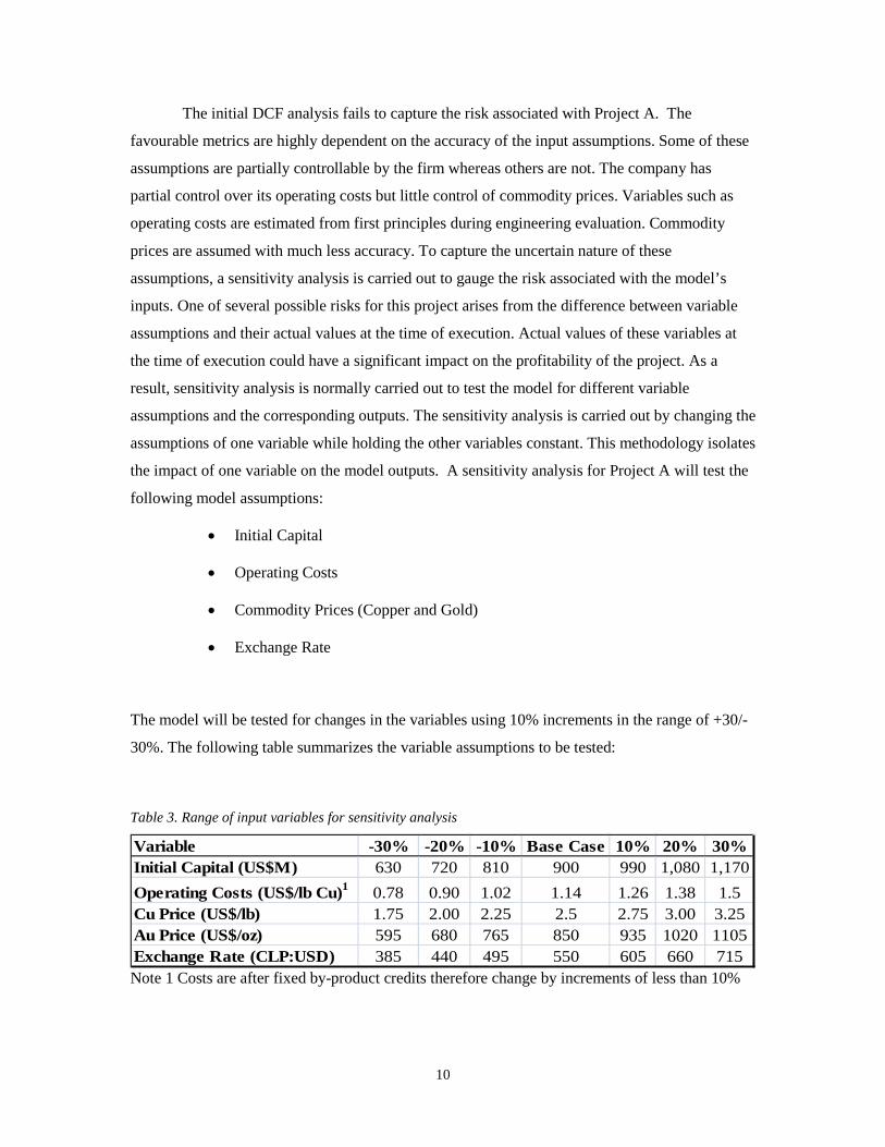
Table 3. Range of input variables for sensitivity analysis
Variable -30% -20% -10% Base Case 10% 20% 30%Initial Capital (US$M) 630 720 810 900 990 1,080 1,170Operating Costs (US$/lb Cu)1 0.78 0.90 1.02 1.14 1.26 1.38 1.5Cu Price (US$/lb) 1.75 2.00 2.25 2.5 2.75 3.00 3.25Au Price (US$/oz) 595 680 765 850 935 1020 1105Exchange Rate (CLP:USD) 385 440 495 550 605 660 715Note 1 Costs are after fixed by-product credits therefore change by increments of less than 10%
11
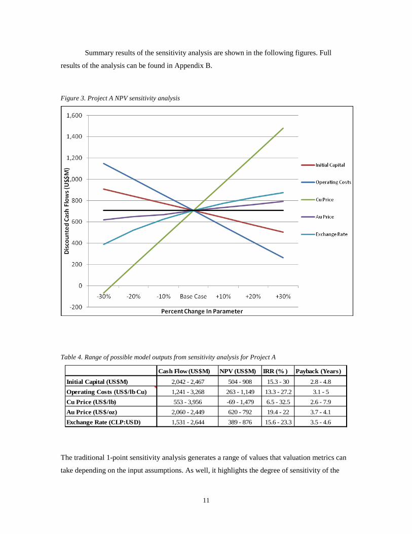
Summary results of the sensitivity analysis are shown in the following figures. Full
results of the analysis can be found in Appendix B.
Figure 3. Project A NPV sensitivity analysis
Table 4. Range of possible model outputs from sensitivity analysis for Project A
Cash Flow (US$M) NPV (US$M) IRR (% ) Payback (Years)
Initial Capital (US$M) 2,042 - 2,467 504 - 908 15.3 - 30 2.8 - 4.8Operating Costs (US$/lb Cu) 1,241 - 3,268 263 - 1,149 13.3 - 27.2 3.1 - 5Cu Price (US$/lb) 553 - 3,956 -69 - 1,479 6.5 - 32.5 2.6 - 7.9Au Price (US$/oz) 2,060 - 2,449 620 - 792 19.4 - 22 3.7 - 4.1Exchange Rate (CLP:USD) 1,531 - 2,644 389 - 876 15.6 - 23.3 3.5 - 4.6
The traditional 1-point sensitivity analysis generates a range of values that valuation metrics can
take depending on the input assumptions. As well, it highlights the degree of sensitivity of the
12
model to one variable relative to others. This analysis shows that the selected valuation metrics
for Project A are most sensitive to the price of copper followed by operating costs. NPV of the
project ranges between -$69M for the worst case copper price scenario and $1,479M for the best
case copper price scenario.
Project B is also a potential copper and molybdenum open pit mine located in Chile. This
project is larger and has a greater degree of complexity than Project A and is at an earlier stage of
development. It will take approximately four years for Project B to reach commercial production.
The capital requirements are an order of magnitude larger compared with Project A. Over the
course of a 20 year mine life, this mine is expected to produce two concentrates: copper and
molybdenum. Small quantities of silver are present in the copper concentrate. The silver
quantities are large enough to be payable by smelters. Both concentrates are expected to be
marketed on the international market. The deterministic valuation basis and methodology are the
same as described earlier for Project A. A summary of the financial model is included in
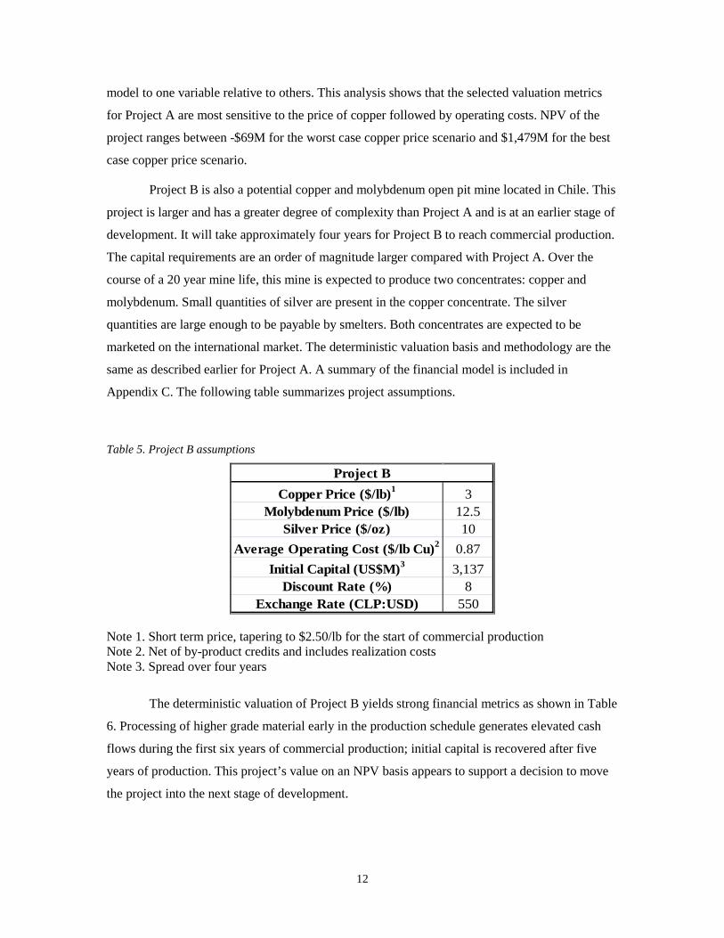
Appendix C. The following table summarizes project assumptions.
Table 5. Project B assumptions
Copper Price ($/lb)1 3Molybdenum Price ($/lb) 12.5
Silver Price ($/oz) 10Average Operating Cost ($/lb Cu)2 0.87
Initial Capital (US$M)3 3,137Discount Rate (%) 8
Exchange Rate (CLP:USD) 550
Project B
Note 1. Short term price, tapering to $2.50/lb for the start of commercial production Note 2. Net of by-product credits and includes realization costs Note 3. Spread over four years
The deterministic valuation of Project B yields strong financial metrics as shown in Table
6. Processing of higher grade material early in the production schedule generates elevated cash
flows during the first six years of commercial production; initial capital is recovered after five
years of production. This project’s value on an NPV basis appears to support a decision to move
the project into the next stage of development.

13
Table 6. Financial performance of Project B
Valuation Methodology DeterministicUndiscounted Cashflows (US$M) 7,113
NPV @ 8% (US$M) 1,249IRR (%) 13.1
Payback (Years) 5.2
Project B
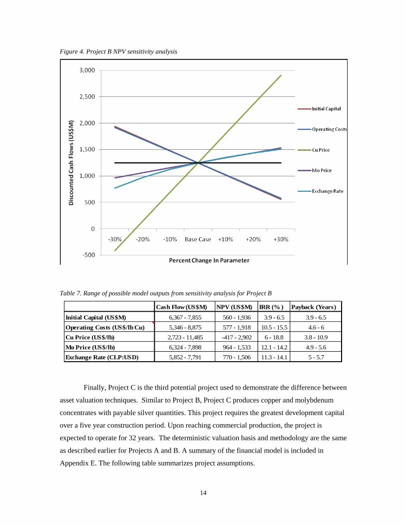
Figure 4 shows a sensitivity analysis of the NPV. The price of copper clearly has the biggest
impact on the value of the project. In fact, the NPV is negative at the lower range of tested copper
prices. Capital and operating costs have similar impacts on the NPV and are the next most
influential variables. The project is least sensitive to the price of molybdenum and the Chilean
peso exchange rate. The influence of the Chilean peso exchange rate on the profitability of the
project is through the conversion of the domestic portion of operating costs to a US dollar basis.
Table 7 summarizes the range of possible values of the financial metrics resulting from a 1-point
sensitivity analysis. The full analysis can be found in Appendix D.
14
Figure 4. Project B NPV sensitivity analysis
Table 7. Range of possible model outputs from sensitivity analysis for Project B
Cash Flow (US$M) NPV (US$M) IRR (% ) Payback (Years)
Initial Capital (US$M) 6,367 - 7,855 560 - 1,936 3.9 - 6.5 3.9 - 6.5Operating Costs (US$/lb Cu) 5,346 - 8,875 577 - 1,918 10.5 - 15.5 4.6 - 6Cu Price (US$/lb) 2,723 - 11,485 -417 - 2,902 6 - 18.8 3.8 - 10.9Mo Price (US$/lb) 6,324 - 7,898 964 - 1,533 12.1 - 14.2 4.9 - 5.6Exchange Rate (CLP:USD) 5,852 - 7,791 770 - 1,506 11.3 - 14.1 5 - 5.7
Finally, Project C is the third potential project used to demonstrate the difference between
asset valuation techniques. Similar to Project B, Project C produces copper and molybdenum
concentrates with payable silver quantities. This project requires the greatest development capital
over a five year construction period. Upon reaching commercial production, the project is
expected to operate for 32 years. The deterministic valuation basis and methodology are the same
as described earlier for Projects A and B. A summary of the financial model is included in
Appendix E. The following table summarizes project assumptions.
15
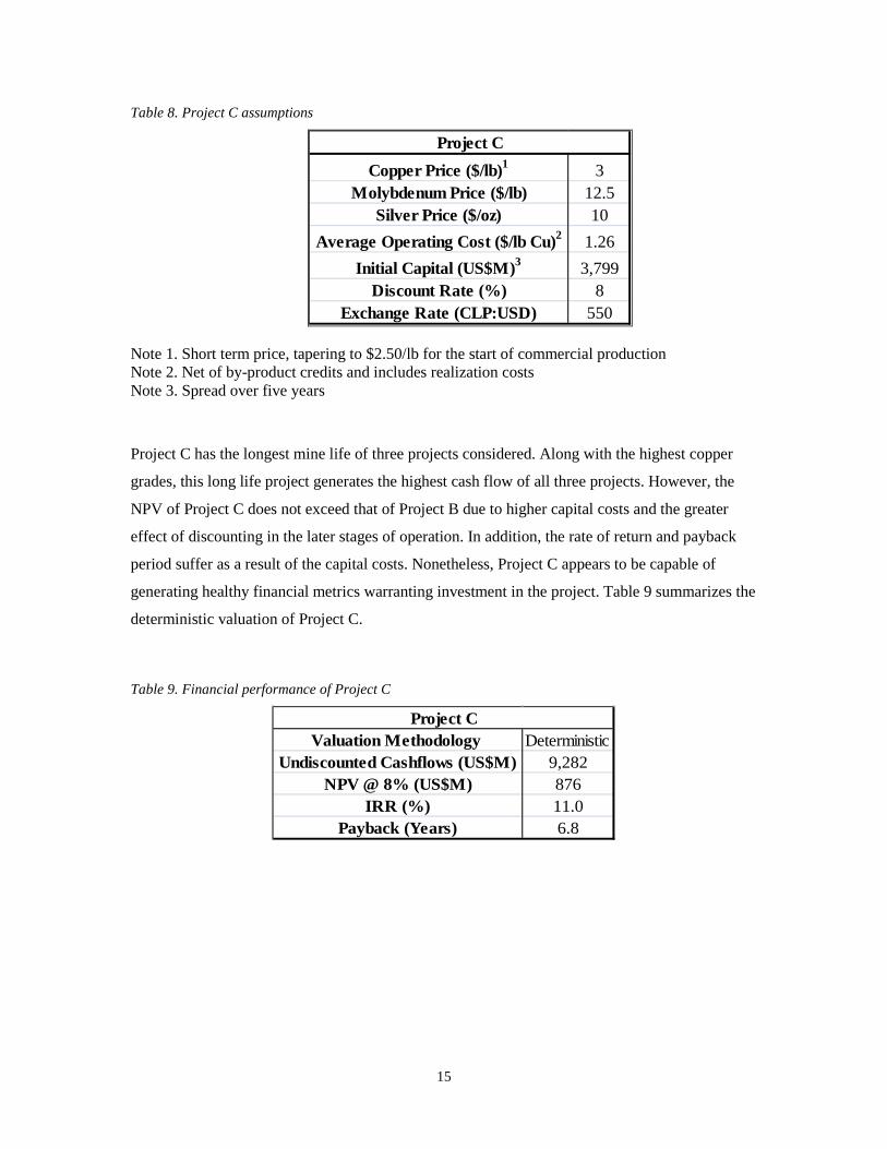
Table 8. Project C assumptions
Copper Price ($/lb)1 3Molybdenum Price ($/lb) 12.5
Silver Price ($/oz) 10Average Operating Cost ($/lb Cu)2 1.26
Initial Capital (US$M)3 3,799Discount Rate (%) 8
Exchange Rate (CLP:USD) 550
Project C
Note 1. Short term price, tapering to $2.50/lb for the start of commercial production Note 2. Net of by-product credits and includes realization costs Note 3. Spread over five years
Project C has the longest mine life of three projects considered. Along with the highest copper
grades, this long life project generates the highest cash flow of all three projects. However, the
NPV of Project C does not exceed that of Project B due to higher capital costs and the greater
effect of discounting in the later stages of operation. In addition, the rate of return and payback
period suffer as a result of the capital costs. Nonetheless, Project C appears to be capable of
generating healthy financial metrics warranting investment in the project. Table 9 summarizes the
deterministic valuation of Project C.
Table 9. Financial performance of Project C
Valuation Methodology DeterministicUndiscounted Cashflows (US$M) 9,282
NPV @ 8% (US$M) 876IRR (%) 11.0
Payback (Years) 6.8
Project C
16
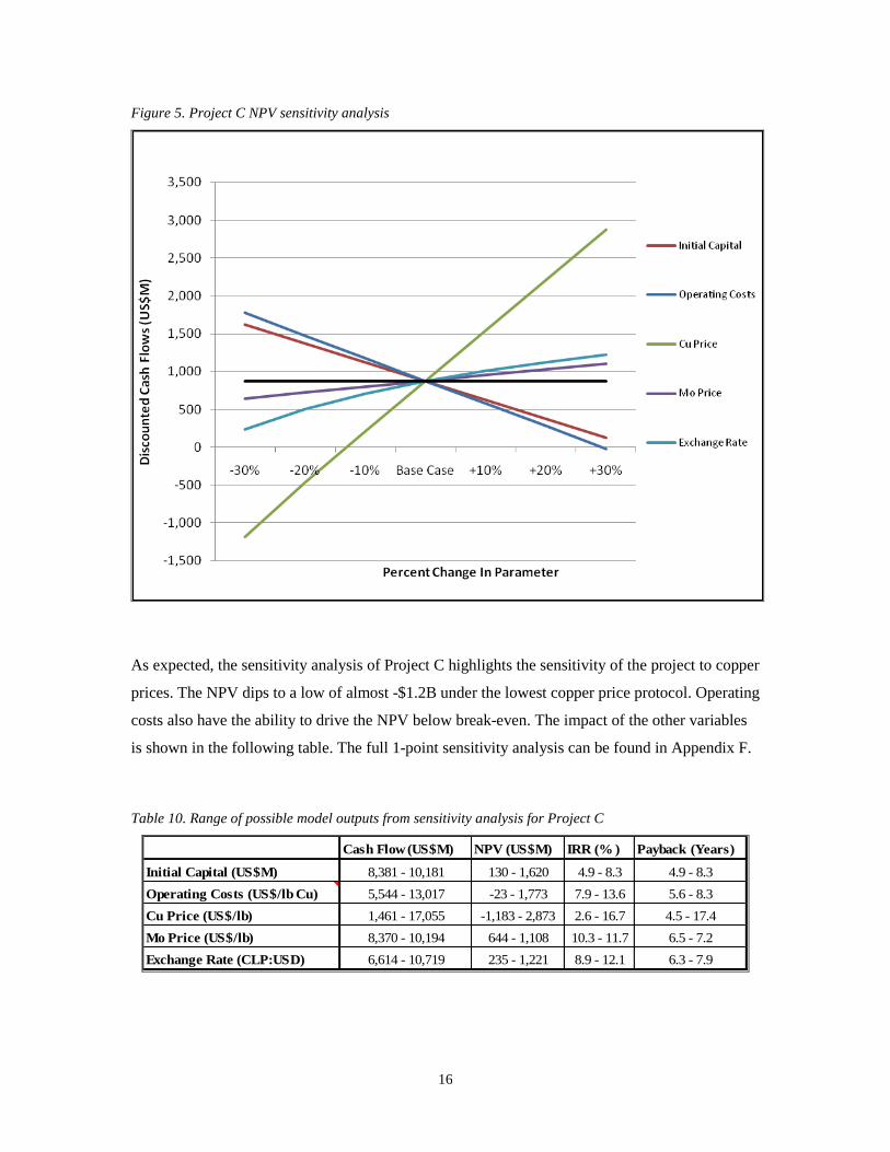
Figure 5. Project C NPV sensitivity analysis
As expected, the sensitivity analysis of Project C highlights the sensitivity of the project to copper
prices. The NPV dips to a low of almost -$1.2B under the lowest copper price protocol. Operating
costs also have the ability to drive the NPV below break-even. The impact of the other variables
is shown in the following table. The full 1-point sensitivity analysis can be found in Appendix F.
Table 10. Range of possible model outputs from sensitivity analysis for Project C
Cash Flow (US$M) NPV (US$M) IRR (% ) Payback (Years)
Initial Capital (US$M) 8,381 - 10,181 130 - 1,620 4.9 - 8.3 4.9 - 8.3Operating Costs (US$/lb Cu) 5,544 - 13,017 -23 - 1,773 7.9 - 13.6 5.6 - 8.3Cu Price (US$/lb) 1,461 - 17,055 -1,183 - 2,873 2.6 - 16.7 4.5 - 17.4Mo Price (US$/lb) 8,370 - 10,194 644 - 1,108 10.3 - 11.7 6.5 - 7.2Exchange Rate (CLP:USD) 6,614 - 10,719 235 - 1,221 8.9 - 12.1 6.3 - 7.9
17
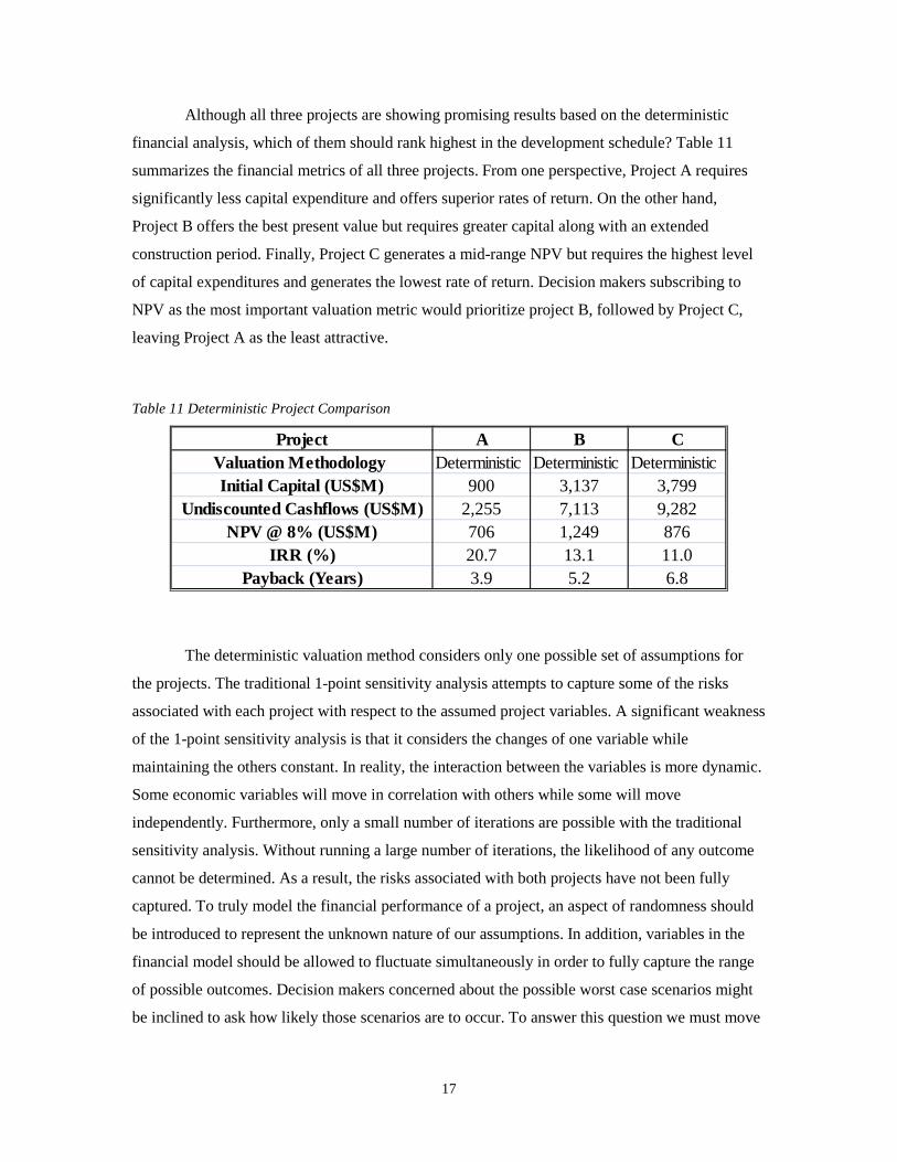
Although all three projects are showing promising results based on the deterministic
financial analysis, which of them should rank highest in the development schedule? Table 11
summarizes the financial metrics of all three projects. From one perspective, Project A requires
significantly less capital expenditure and offers superior rates of return. On the other hand,
Project B offers the best present value but requires greater capital along with an extended
construction period. Finally, Project C generates a mid-range NPV but requires the highest level
of capital expenditures and generates the lowest rate of return. Decision makers subscribing to
NPV as the most important valuation metric would prioritize project B, followed by Project C,
leaving Project A as the least attractive.
Table 11 Deterministic Project Comparison
Project A B CValuation Methodology Deterministic Deterministic DeterministicInitial Capital (US$M) 900 3,137 3,799
Undiscounted Cashflows (US$M) 2,255 7,113 9,282NPV @ 8% (US$M) 706 1,249 876
IRR (%) 20.7 13.1 11.0Payback (Years) 3.9 5.2 6.8
The deterministic valuation method considers only one possible set of assumptions for
the projects. The traditional 1-point sensitivity analysis attempts to capture some of the risks
associated with each project with respect to the assumed project variables. A significant weakness
of the 1-point sensitivity analysis is that it considers the changes of one variable while
maintaining the others constant. In reality, the interaction between the variables is more dynamic.
Some economic variables will move in correlation with others while some will move
independently. Furthermore, only a small number of iterations are possible with the traditional
sensitivity analysis. Without running a large number of iterations, the likelihood of any outcome
cannot be determined. As a result, the risks associated with both projects have not been fully
captured. To truly model the financial performance of a project, an aspect of randomness should
be introduced to represent the unknown nature of our assumptions. In addition, variables in the
financial model should be allowed to fluctuate simultaneously in order to fully capture the range
of possible outcomes. Decision makers concerned about the possible worst case scenarios might
be inclined to ask how likely those scenarios are to occur. To answer this question we must move

18
beyond the deterministic financial model and 1-point sensitivity analysis and introduce a
probabilistic financial model.
19
4.0 Probabilistic Asset Valuation
A variable is modelled stochastically if a random process predicts its future behaviour, at
least in part16. A probabilistic approach to asset valuation attempts to incorporate the influence of
random behaviour in some or all of the variables. Using behaviour models, like those introduced
earlier, and Monte Carlo simulation, a financial model can be tested for many possible scenarios.
Running many iterations allows the user to develop a probability distribution of the model’s
outputs. This probability distribution provides decision makers with the additional information
not afforded to them by the simple 1-point sensitivity analysis described in the previous section.
Furthermore, behaviour of dependant variables can be correlated with other variables to develop a
more realistic situational analysis. For example, probabilistic modelling was utilized for the
prominent Oyu Tolgoil project in Mongolia17. Stochastic metal price forecasts were developed to
capture cash flow uncertainty of this $4.6 billion dollar project. The use of probabilistic models
takes the user towards the dynamic modelling of uncertainty as described in the Banff Taxonomy.
This migration is evident in Figure 1 by an upward movement along the uncertainty axis of
taxonomy. This methodology has been applied to risk analysis with applications beyond financial
modelling. PRA is a general methodology used as a support tool to help quantify the risks
inherent with uncertain processes18
To transform the deterministic models developed in the previous section into
probabilistic models, select variables will be modelled stochastically. For simplicity and
demonstrative purposes, one variable will be modelled stochastically and the behaviour of
another will be predicted through its correlation with the stochastic variable. The traditional
sensitivity analysis identified the price of copper and operating costs as having significant
influence on the financial model’s outputs. As a result, the price of copper will be modelled
stochastically. Operating costs will fluctuate due to the exchange rate correlation with the price of
copper. This probabilistic financial model will be better suited to understanding the financial
performance of all three projects.
.
16 Dixit & Pindyck, 1994, p. 60 17 Oyu Tolgoil Technical Report, 2010, p. 44-47 18 Bedford & Cooke, 2001, p. 3
20
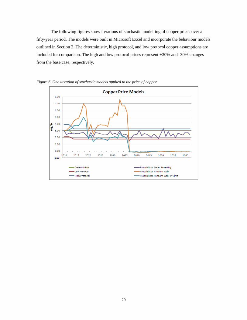
The following figures show iterations of stochastic modelling of copper prices over a
fifty-year period. The models were built in Microsoft Excel and incorporate the behaviour models
outlined in Section 2. The deterministic, high protocol, and low protocol copper assumptions are
included for comparison. The high and low protocol prices represent +30% and -30% changes
from the base case, respectively.
Figure 6. One iteration of stochastic models applied to the price of copper
21
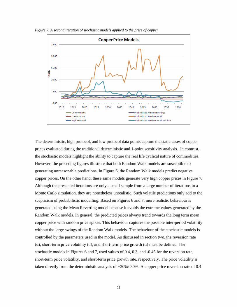
Figure 7. A second iteration of stochastic models applied to the price of copper
The deterministic, high protocol, and low protocol data points capture the static cases of copper
prices evaluated during the traditional deterministic and 1-point sensitivity analysis. In contrast,
the stochastic models highlight the ability to capture the real life cyclical nature of commodities.
However, the preceding figures illustrate that both Random Walk models are susceptible to
generating unreasonable predictions. In Figure 6, the Random Walk models predict negative
copper prices. On the other hand, these same models generate very high copper prices in Figure 7.
Although the presented iterations are only a small sample from a large number of iterations in a
Monte Carlo simulation, they are nonetheless unrealistic. Such volatile predictions only add to the
scepticism of probabilistic modelling. Based on Figures 6 and 7, more realistic behaviour is
generated using the Mean Reverting model because it avoids the extreme values generated by the
Random Walk models. In general, the predicted prices always trend towards the long term mean
copper price with random price spikes. This behaviour captures the possible inter-period volatility
without the large swings of the Random Walk models. The behaviour of the stochastic models is
controlled by the parameters used in the model. As discussed in section two, the reversion rate
(α), short-term price volatility (σ), and short-term price growth (α) must be defined. The
stochastic models in Figures 6 and 7, used values of 0.4, 0.3, and -0.45 for the reversion rate,
short-term price volatility, and short-term price growth rate, respectively. The price volatility is
taken directly from the deterministic analysis of +30%/-30%. A copper price reversion rate of 0.4
22
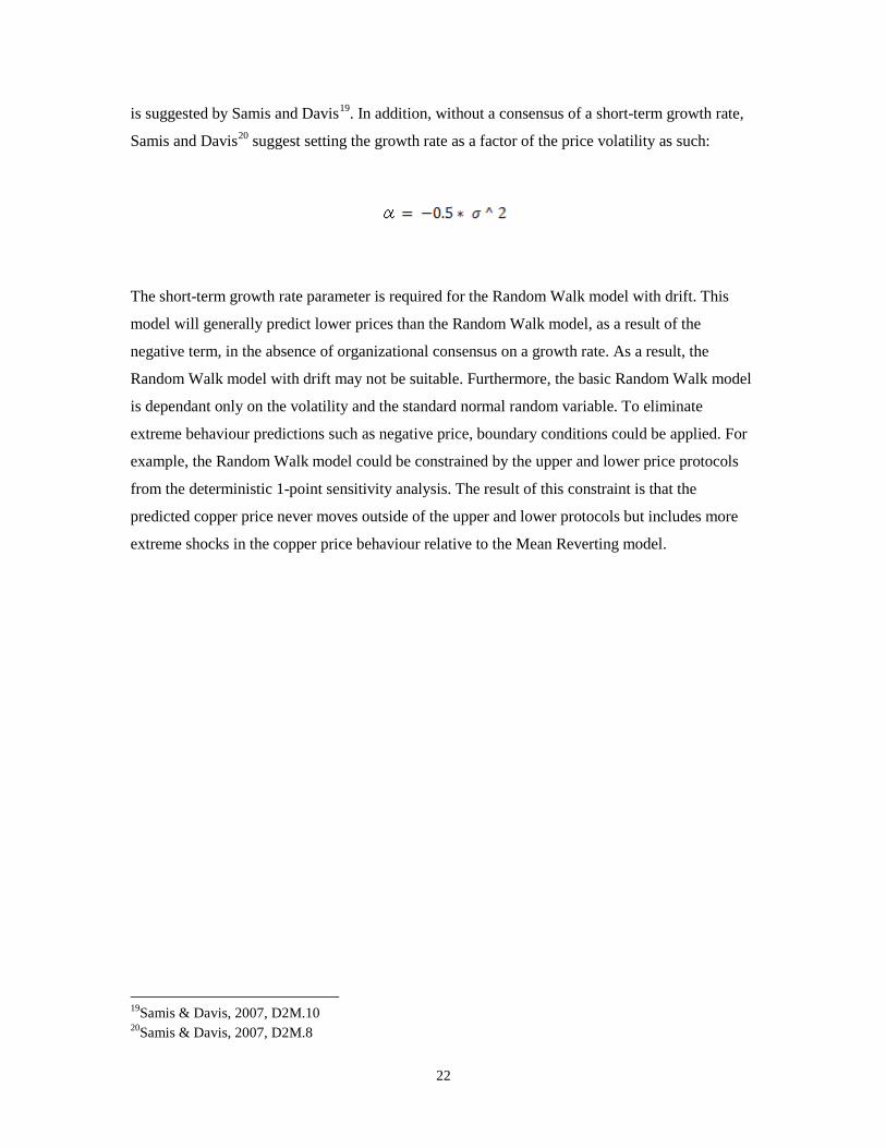
is suggested by Samis and Davis19. In addition, without a consensus of a short-term growth rate,
Samis and Davis20
suggest setting the growth rate as a factor of the price volatility as such:
The short-term growth rate parameter is required for the Random Walk model with drift. This
model will generally predict lower prices than the Random Walk model, as a result of the
negative term, in the absence of organizational consensus on a growth rate. As a result, the
Random Walk model with drift may not be suitable. Furthermore, the basic Random Walk model
is dependant only on the volatility and the standard normal random variable. To eliminate
extreme behaviour predictions such as negative price, boundary conditions could be applied. For
example, the Random Walk model could be constrained by the upper and lower price protocols
from the deterministic 1-point sensitivity analysis. The result of this constraint is that the
predicted copper price never moves outside of the upper and lower protocols but includes more
extreme shocks in the copper price behaviour relative to the Mean Reverting model.
19Samis & Davis, 2007, D2M.10 20Samis & Davis, 2007, D2M.8
23
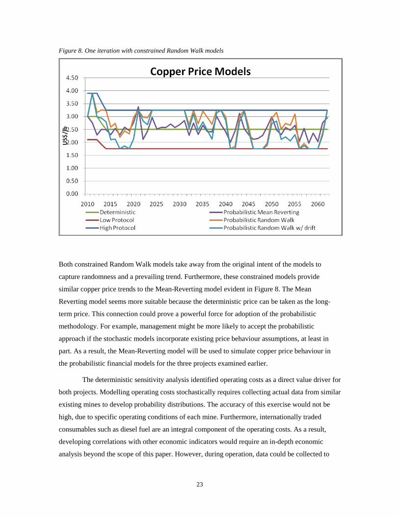
Figure 8. One iteration with constrained Random Walk models
Both constrained Random Walk models take away from the original intent of the models to
capture randomness and a prevailing trend. Furthermore, these constrained models provide
similar copper price trends to the Mean-Reverting model evident in Figure 8. The Mean
Reverting model seems more suitable because the deterministic price can be taken as the long-
term price. This connection could prove a powerful force for adoption of the probabilistic
methodology. For example, management might be more likely to accept the probabilistic
approach if the stochastic models incorporate existing price behaviour assumptions, at least in
part. As a result, the Mean-Reverting model will be used to simulate copper price behaviour in
the probabilistic financial models for the three projects examined earlier.
The deterministic sensitivity analysis identified operating costs as a direct value driver for
both projects. Modelling operating costs stochastically requires collecting actual data from similar
existing mines to develop probability distributions. The accuracy of this exercise would not be
high, due to specific operating conditions of each mine. Furthermore, internationally traded
consumables such as diesel fuel are an integral component of the operating costs. As a result,
developing correlations with other economic indicators would require an in-depth economic
analysis beyond the scope of this paper. However, during operation, data could be collected to
24
develop a probability distribution for operating costs based on historical performance. As a result,
modelling operating costs stochastically would be more practical once a project is in operation.
Even though we will not model operating costs in our probabilistic model directly, we
can incorporate their influence indirectly. Operating cost cash outflows occur in both domestic
and foreign currencies. Disbursements for labour and electricity take place in domestic Chilean
pesos. The remainder of the operating costs are for internationally traded goods and services and
are typically paid in US dollars. The division between costs realized in domestic and foreign
currencies is approximately even. As a result, the fluctuations in the Chilean peso exchange rates
have a direct influence on total operating costs, on a US dollar basis. Therefore, exchange rates
influence net cash flows for Project A. A government’s monetary policy controls the behaviour of
its currency’s exchange rate. If the monetary policy were such that it is directing the course of
exchange rate, then predicting its behaviour would require alignment with the government’s
intentions. On the other hand, if exchange rates are free floating, then their behaviour should
correlate well with the economic drivers fuelling the economy. The Chilean economy is very
much reliant on its natural resources, with copper extraction playing a major role. As a result, if
the currency were free floating, we would expect a strong correlation between copper prices and
the Chilean exchange rates. The following figure shows the relationship between copper prices
and the Chilean exchange rates based on daily quotes since 200221
21 LME copper spot prices and Chilean peso exchange rates from 01/01/02 to 01/14/11
.
25
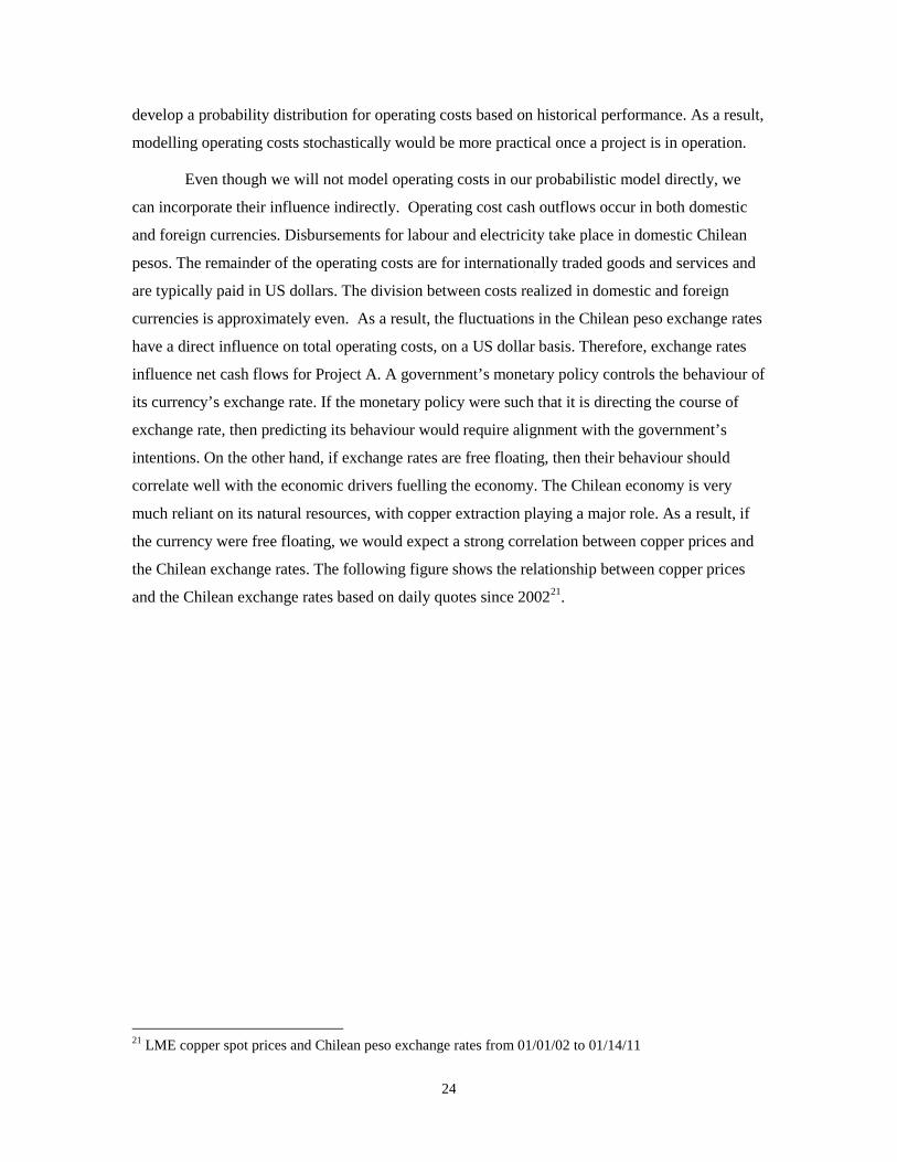
Figure 9. Copper Price and Chilean Peso exchange rate data since 2002
The data shows a good fit with a linear trend line having a coefficient of determination of 0.7903.
Careful consideration of the period used in developing an economic relationship between two
variables is required. Since the relationship will be used to model the future, the historical
economic conditions of the dataset should resemble the expected future economic conditions.
Otherwise, accuracy of the predicative model would be questionable. The period between 2002
and the beginning of 2011 is assumed to be a reasonable estimation of the future economic
conditions because it captures a full economic cycle. Economic conditions were on the rebound in
2002 following the terrorist attacks in the United States before beginning to deteriorate in 2008 in
advance of the most recent recession. A gradual recovery began to take shape in the second half
of 2009, continuing through 2010.
Now that we have defined the stochastic model for the price of copper and correlated the
behaviour of the Chilean exchange rate, we can develop probabilistic financial models for
Projects A, B, and C. The Crystal Ball software was used to carry out Monte Carlo simulation
with 100,000 iterations. This number of iterations far exceeds the sample size required to achieve
statistically valid outputs – 95% confidence level with a 5% confidence interval. The Crystal Ball
26
software was selected due to existing user knowledge within Teck, ease of use (Microsoft Excel
add-in), and superior presentation of results. Results of the Monte Carlo simulations will be
shown as histograms of NPV, IRR, and payback period. The histograms show the probability
(primary vertical axis) and frequency (secondary vertical axis) of values occurring in a given
interval (horizontal axis). The pink area of each histogram represents intervals which are below
the deterministic value. Conversely, the blue area indicates the intervals which meet or exceed the
deterministic value. In addition, a certainty of meeting or exceeding the deterministic value is
shown. Percentiles and mean values of the results are represented by blue vertical lines; where
P90, P50, and P10 are defined as values which are exceeded by 90%, 50%, and 10% of the
simulation outputs, respectively. Outputs of the simulations for Project A are shown in the
following figures.
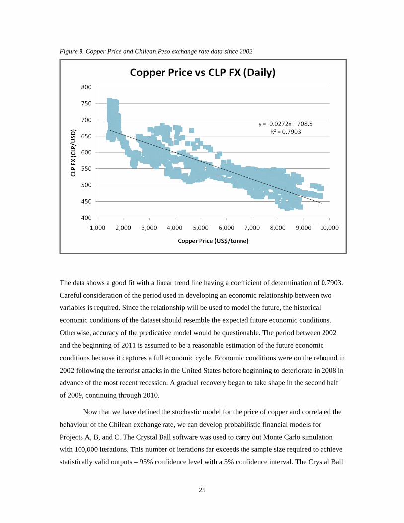
Figure 10. Project A NPV histogram
27
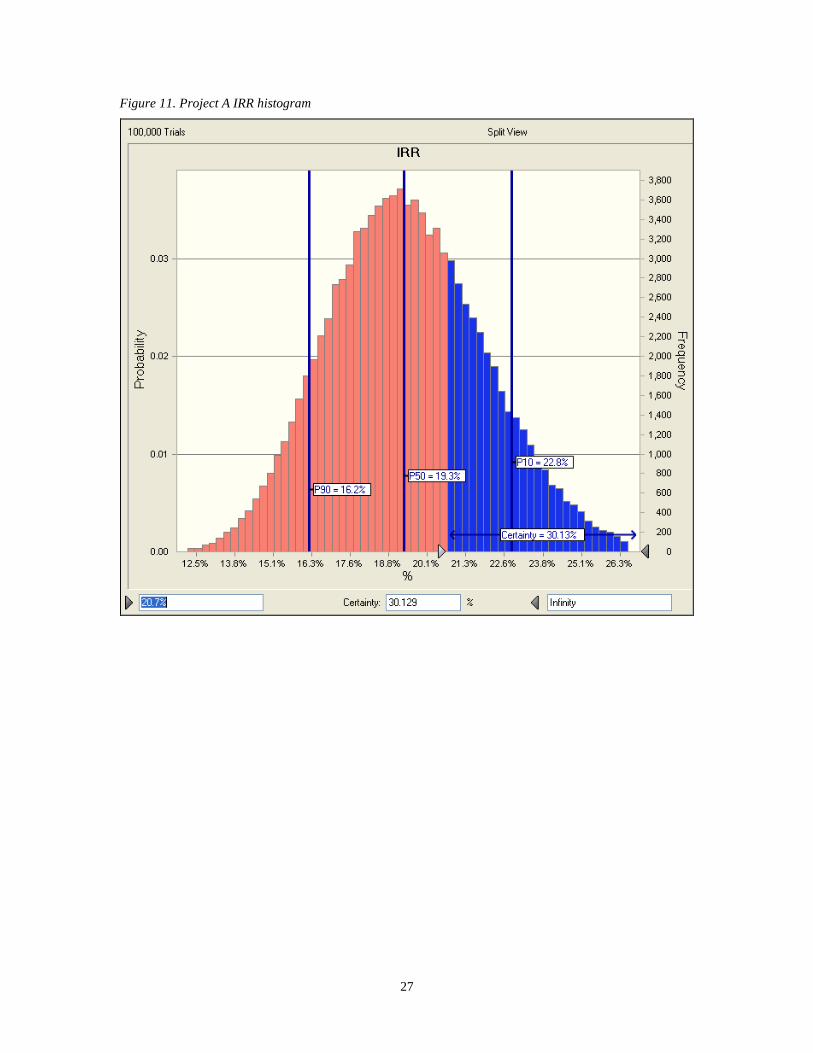
Figure 11. Project A IRR histogram
28
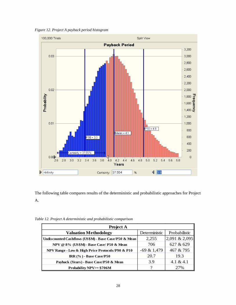
Figure 12. Project A payback period histogram
The following table compares results of the deterministic and probabilistic approaches for Project
A.
Table 12. Project A deterministic and probabilistic comparison
Valuation Methodology Deterministic ProbabilisticUndiscounted Cashflows (US$M) - Base Case/P50 & Mean 2,255 2,091 & 2,095
NPV @ 8% (US$M) - Base Case/ P50 & Mean 706 627 & 629NPV Range - Low & High Price Protocols/P90 & P10 -69 & 1,479 467 & 795
IRR (% ) - Base Case/P50 20.7 19.3Payback (Years) - Base Case/P50 & Mean 3.9 4.1 & 4.1
Probability NPV>= $706M ? 27%
Project A
29
The probabilistic model has evaluated a large number of copper price scenarios along with the
correlated Chilean Peso exchange rate. As a result, the combined affect can be captured on the
project’s profitability. The deterministic approach identified an NPV of $706M. The probabilistic
analysis returned lower values for undiscounted cash flows, NPV, IRR, and payback period. The
NPV range shows a significant difference between the two methodologies. The probabilistic
model results in a much tighter range than the deterministic model. This difference can be
explained by the application of a correlated variable. The NPV range in the deterministic model
considered only the low and high copper price protocols. On the other hand, the probabilistic
model included the correlated exchange rate behaviour for each simulated copper price. This has
a dampening effect on the NPV during years with lower copper prices. On a US dollar basis,
lower copper prices correspond with reduced operating costs, and vice-versa, as a result of the
fluctuating Chilean peso exchange rate. These types of cause and effect relationships more
closely model real life economic conditions.
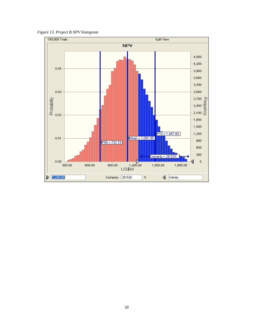
The Monte Carlo simulation of the probabilistic financial model for Project B
incorporates the same parameters as the simulation of Project A (number of iterations, Mean
Reverting copper price model, Chilean peso and copper price correlation, rate of reversion, and
copper price volatility). Histograms of the simulation for NPV, IRR, and payback period are
shown in the following figures.
30
Figure 13. Project B NPV histogram
31
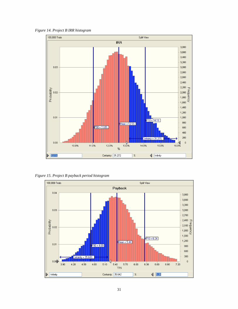
Figure 14. Project B IRR histogram
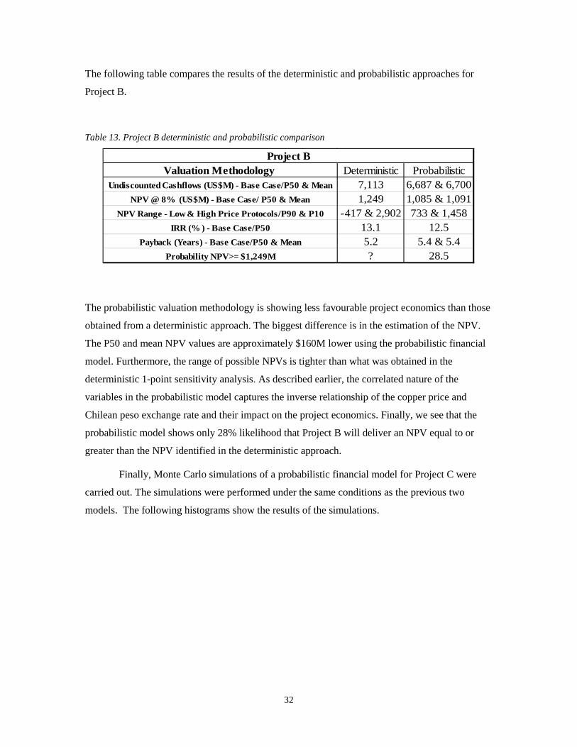
Figure 15. Project B payback period histogram
32
The following table compares the results of the deterministic and probabilistic approaches for
Project B.
Table 13. Project B deterministic and probabilistic comparison
Valuation Methodology Deterministic ProbabilisticUndiscounted Cashflows (US$M) - Base Case/P50 & Mean 7,113 6,687 & 6,700
NPV @ 8% (US$M) - Base Case/ P50 & Mean 1,249 1,085 & 1,091NPV Range - Low & High Price Protocols/P90 & P10 -417 & 2,902 733 & 1,458
IRR (% ) - Base Case/P50 13.1 12.5Payback (Years) - Base Case/P50 & Mean 5.2 5.4 & 5.4
Probability NPV>= $1,249M ? 28.5
Project B
The probabilistic valuation methodology is showing less favourable project economics than those
obtained from a deterministic approach. The biggest difference is in the estimation of the NPV.
The P50 and mean NPV values are approximately $160M lower using the probabilistic financial
model. Furthermore, the range of possible NPVs is tighter than what was obtained in the
deterministic 1-point sensitivity analysis. As described earlier, the correlated nature of the
variables in the probabilistic model captures the inverse relationship of the copper price and
Chilean peso exchange rate and their impact on the project economics. Finally, we see that the
probabilistic model shows only 28% likelihood that Project B will deliver an NPV equal to or
greater than the NPV identified in the deterministic approach.
Finally, Monte Carlo simulations of a probabilistic financial model for Project C were
carried out. The simulations were performed under the same conditions as the previous two
models. The following histograms show the results of the simulations.
33
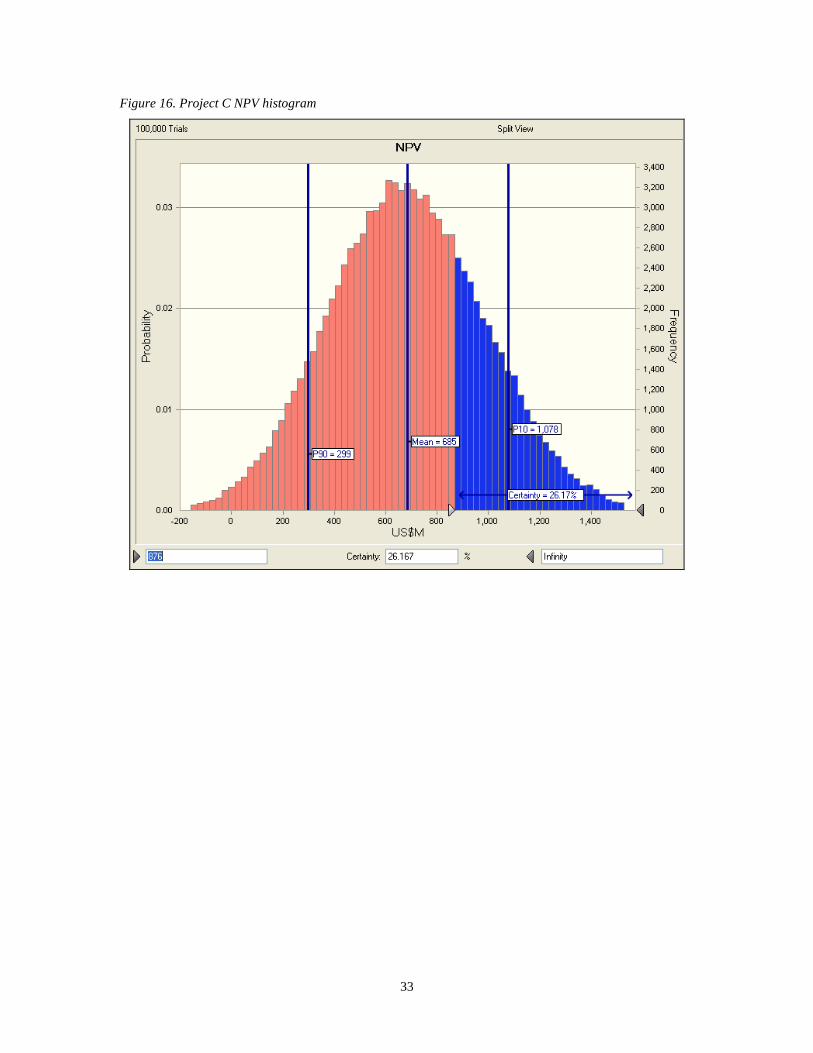
Figure 16. Project C NPV histogram
34
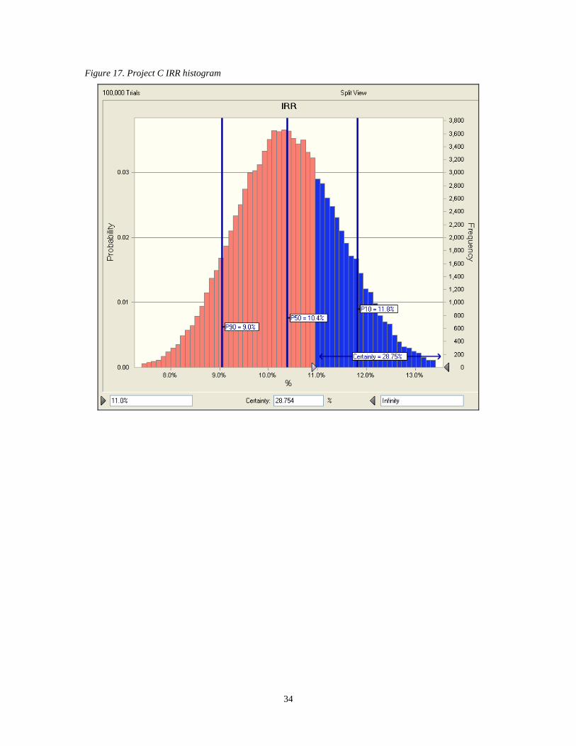
Figure 17. Project C IRR histogram
35
Figure 18. Project C payback period histogram
The following table compares the results of the deterministic and probabilistic approaches for
Project C.
Table 14. Project C deterministic and probabilistic comparison
Valuation Methodology Deterministic ProbabilisticUndiscounted Cashflows (US$M) - Base Case/P50 & Mean 9,282 8,554 & 8,565
NPV @ 8% (US$M) - Base Case/ P50 & Mean 876 679 & 685NPV Range - Low & High Price Protocols/P90 & P10 -1,183 & 2,873 299 & 1,078
IRR (% ) - Base Case/P50 11.0 10.4Payback (Years) - Base Case/P50 & Mean 6.8 7.2 & 7.2
Probability NPV>= $876M ? 26
Project C

36
Results consistent with the previous projects are seen from the probabilistic model applied to
Project C. Most model outputs underestimate the values derived by the deterministic model. An
exception is the NPV range, which is again much tighter in the probabilistic case.
We have not explored the impact of parameters, such as reversion and volatility, used in
the probabilistic model. The volatility parameter is taken directly from the original deterministic
analysis. The deterministic sensitivity analysis tested copper prices of +30% and -30% from the
assumed base case prices. As a result, a volatility value of 0.3 can be considered to be a good
input into the probabilistic model. However, current deterministic practices do not give any
indication about the reversion parameter that might be appropriate. The reversion parameter
describes how quickly a variable returns to the equilibrium level and is inversely related to the
time it takes deviations to return to the equilibrium level. Therefore smaller values indicate longer
reversion times and vice versa. To test the impact of the reversion parameter on model outputs, a
range of values was tested. The following figure summarizes the model outputs using different
assumptions for the reversion parameter on Projects A, B, and C.
37
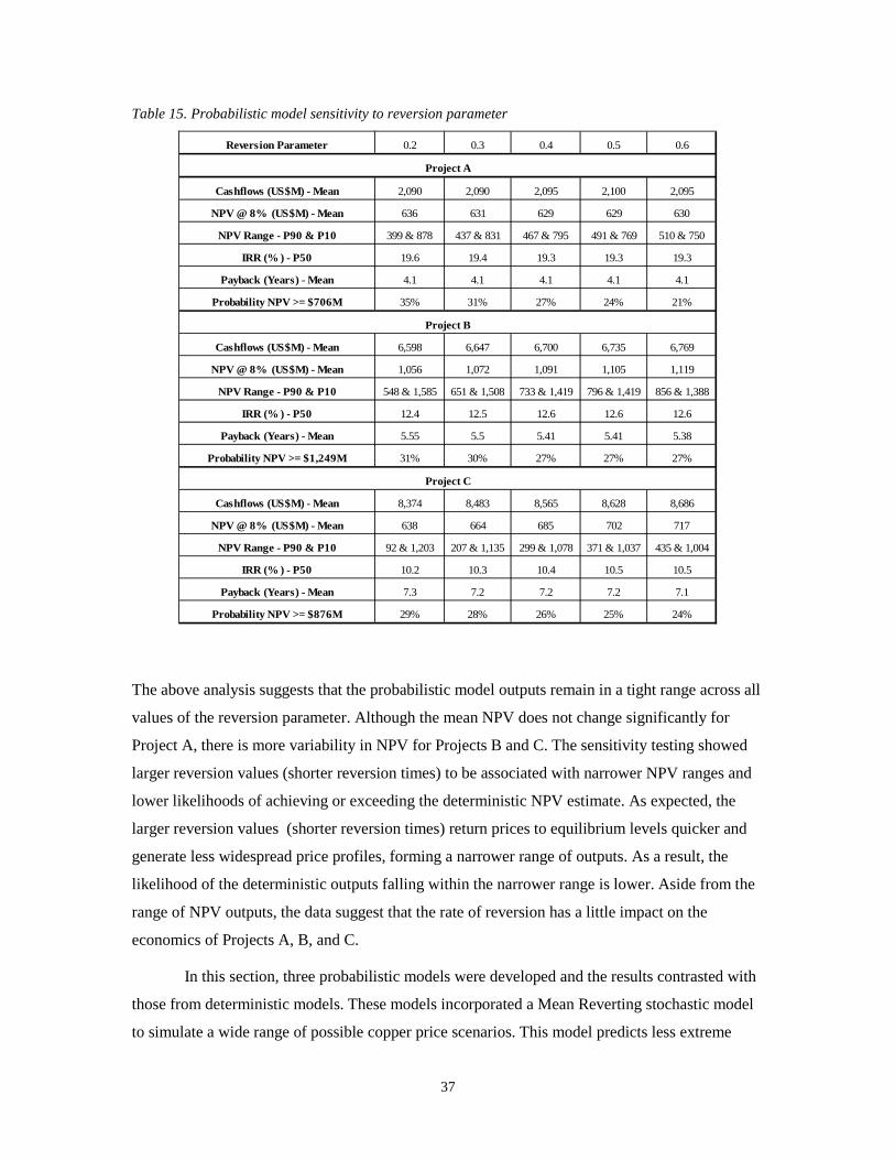
Table 15. Probabilistic model sensitivity to reversion parameter
Reversion Parameter 0.2 0.3 0.4 0.5 0.6
Cashflows (US$M) - Mean 2,090 2,090 2,095 2,100 2,095
NPV @ 8% (US$M) - Mean 636 631 629 629 630
NPV Range - P90 & P10 399 & 878 437 & 831 467 & 795 491 & 769 510 & 750
IRR (% ) - P50 19.6 19.4 19.3 19.3 19.3
Payback (Years) - Mean 4.1 4.1 4.1 4.1 4.1
Probability NPV >= $706M 35% 31% 27% 24% 21%
Cashflows (US$M) - Mean 6,598 6,647 6,700 6,735 6,769
NPV @ 8% (US$M) - Mean 1,056 1,072 1,091 1,105 1,119
NPV Range - P90 & P10 548 & 1,585 651 & 1,508 733 & 1,419 796 & 1,419 856 & 1,388
IRR (% ) - P50 12.4 12.5 12.6 12.6 12.6
Payback (Years) - Mean 5.55 5.5 5.41 5.41 5.38
Probability NPV >= $1,249M 31% 30% 27% 27% 27%
Cashflows (US$M) - Mean 8,374 8,483 8,565 8,628 8,686
NPV @ 8% (US$M) - Mean 638 664 685 702 717
NPV Range - P90 & P10 92 & 1,203 207 & 1,135 299 & 1,078 371 & 1,037 435 & 1,004
IRR (% ) - P50 10.2 10.3 10.4 10.5 10.5
Payback (Years) - Mean 7.3 7.2 7.2 7.2 7.1
Probability NPV >= $876M 29% 28% 26% 25% 24%
Project A
Project B
Project C
The above analysis suggests that the probabilistic model outputs remain in a tight range across all
values of the reversion parameter. Although the mean NPV does not change significantly for
Project A, there is more variability in NPV for Projects B and C. The sensitivity testing showed
larger reversion values (shorter reversion times) to be associated with narrower NPV ranges and
lower likelihoods of achieving or exceeding the deterministic NPV estimate. As expected, the
larger reversion values (shorter reversion times) return prices to equilibrium levels quicker and
generate less widespread price profiles, forming a narrower range of outputs. As a result, the
likelihood of the deterministic outputs falling within the narrower range is lower. Aside from the
range of NPV outputs, the data suggest that the rate of reversion has a little impact on the
economics of Projects A, B, and C.
In this section, three probabilistic models were developed and the results contrasted with
those from deterministic models. These models incorporated a Mean Reverting stochastic model
to simulate a wide range of possible copper price scenarios. This model predicts less extreme
38
copper price values than the Random Walk models and incorporates assumptions from the
deterministic approach. The static copper price assumption from the deterministic model was
used as the long term price to which copper prices revert in the probabilistic model. In addition,
the volatility parameter required for the probabilistic model was based on the range of copper
prices tested with the deterministic 1-point sensitivity analysis. The use of established parameters
in the probabilistic model provides a connection with familiar processes which could assist in
adoption of the probabilistic methodology. Furthermore, behaviour of the Chilean Peso exchange
rate was correlated with the price of copper. As a result, the ability to capture the impacts of
realistic behaviour due to inter related variables was demonstrated. In general, comparison of the
deterministic and probabilistic methodologies shows that the valuation metrics are less favourable
for the example projects when probabilistic models were used. The influence of variable copper
price profiles and correlated exchange rate behaviour resulted in lower average values compared
with the absolute deterministic outputs. The simulation approach of probabilistic financial
modelling has introduced a new metric to the valuation toolkit: probability. The likelihood of
achieving certain metrics, or ranges, can now be utilized in evaluating and comparing projects.
The next section explores the application of information generated from the probabilistic models.
39
5.0 Application
The probabilistic models have taken risk analysis beyond the capabilities of the
deterministic models. More simplistically, a deterministic model, along with the 1-point
sensitivity analysis, only affords the ability to test a limited number of variable combinations. The
probabilistic approach is most ideally suited either to marginal projects where the sensitivity to
input variables is high, or to projects with a high degree of complexity. In both cases, evaluating a
large number of iterations assists in better understanding the project risks.
The main application of probabilistic modelling is to ascertain the uncertainty of cash
flows generated from a project. The methodology can be applied to a single project to gauge risk,
or to a series of projects in order to prioritize alternatives. For a single project, the decision
process would involve evaluating the likelihood that the project generates a positive NPV. In the
case of deciding between multiple projects, the exercise is one of prioritizing. Balancing financial
performance with the risk profiles of alternatives is required to assign priorities. Projects could
appear attractive when evaluated deterministically, but reveal significant risk when evaluated
probabilistically. In the case of the three projects presented in this paper, the application of a
probabilistic model showed that the financial metrics could be overstated using the deterministic
models. The probabilities of achieving or exceeding the deterministic NPVs were approximately
27% for all three projects; the remainder of the Monte Carlo iterations returned lower NPV
values. Although the probabilistic evaluation showed less favourable metrics for all projects,
evaluated individually, each appears to support a decision to advance the projects. Recall that the
deterministic analysis ranked the projects in the following order: B, C, and A. Reconsidering the
order of the projects based on the probabilistic analysis reveals a possible ranking change. Project
B continues to outperform the others on the NPV metric, arguably the most important metric.
However, the difference between average NPVs of Projects A and C is reduced to $55M, still in
favour of Project C. The decision to prefer Project C over Project A is now more difficult
considering the superior rate of return of Project A. As a result, the case could be made that the
order of attractiveness should be Project B, A, and C.
The probabilistic evaluation technique also can be used as a strategic tool. Given the
widespread use of deterministic evaluation, a probabilistic approach generates information
40
possibly not captured by others. As a result, pricing decisions could be aided with this approach
to asset valuation. In our examples earlier, the low likelihoods of achieving the deterministic
NPVs should be taken into consideration when developing proposals or reviewing bids for the
purchase or sale of assets. Significant discounts could be justified when the likelihood of realizing
a stated value is low. On the other hand, high likelihoods could demand prices closer to the
estimated value of the asset.
Marginal projects could benefit from a probabilistic evaluation approach. Projects
showing a significant downside from a 1-point sensitivity analysis face the potential of being held
back on the basis of their risk. A more realistic scenario, where variable behaviour is correlated,
could lessen the negative impact of a worst case scenario. Although not necessarily a marginal
project, Project B highlights this potential benefit. The project was showing NPV ranges of $-
417M to $2,902M deterministically and $733M to $1,458M probabilistically. No longer is the
NPV of the project negative on the extreme low end. In general, the tighter NPV range is a result
of the inverse relationship on the NPV of copper prices and Chilean peso exchange rates.
Although the upside of the project is limited, more importantly, the downside is limited.
The application of probabilistic evaluation has shown that risks inherent in financial
models can be measured quantitatively. Monte Carlo simulations allow the user to determine the
probability with which any given metric is expected to be achieved. In the case of the most
widely used metric, NPV, decision makers are able to consider the chances that a project will
generate a positive NPV. In order to utilize probabilistic asset valuation, acceptance of the
methodology must first take place within the organization. The challenges of this acceptance are
explored in the following section.
41
6.0 Implementation
Implementation of probabilistic asset valuation is not meant to be a substitute for
deterministic asset valuation, rather it is meant to complement the existing deterministic asset
valuation methodology. Nonetheless, showing the potential benefits of this tool does not
guarantee adoption. Existing processes with which company objectives are met are likely to be
deeply rooted within the organization. As a result, if interest exists within the organization to
adopt a new tool, an implementation strategy is required. Two barriers to implementation of
probabilistic asset valuation were identified in section 2 of this paper and include subjectivity and
understanding of the probabilistic process. In this section, attitudes towards probabilistic asset
valuation at Teck are explored and an implementation strategy is derived for the adoption of this
valuation methodology.
To assist in the development of an implementation strategy for the use of probabilistic
asset valuation at Teck, members of Teck’s executive management team were surveyed. Opinions
of builders and users of financial models were solicited. Drawing a large number of firm
conclusions from the survey is not possible due to the limited sample size (5 responses out of a
possible 7). However, the survey can be used to assess high level attitudes toward probabilistic
asset valuation. The first three survey questions focused on gauging the executive management
team’s familiarity with probabilistic valuation and included the following questions:
1.
2.
How would you describe your familiarity with the range of asset valuation techniques?
3.
How would you describe your knowledge about stochastic processes?
Have you ever developed or analyzed the results from a probabilistic asset valuation
model?
Responses to the survey are summarized in the following figure.
42
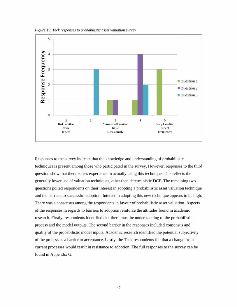
Figure 19. Teck responses to probabilistic asset valuation survey
Responses to the survey indicate that the knowledge and understanding of probabilistic
techniques is present among those who participated in the survey. However, responses to the third
question show that there is less experience in actually using this technique. This reflects the
generally lower use of valuation techniques, other than deterministic DCF. The remaining two
questions polled respondents on their interest in adopting a probabilistic asset valuation technique
and the barriers to successful adoption. Interest in adopting this new technique appears to be high.
There was a consensus among the respondents in favour of probabilistic asset valuation. Aspects
of the responses in regards to barriers to adoption reinforce the attitudes found in academic
research. Firstly, respondents identified that there must be understanding of the probabilistic
process and the model outputs. The second barrier in the responses included consensus and
quality of the probabilistic model inputs. Academic research identified the potential subjectivity
of the process as a barrier to acceptance. Lastly, the Teck respondents felt that a change from
current processes would result in resistance to adoption. The full responses to the survey can be
found in Appendix G.
43
Kotter’s model of change22
provides eight elements necessary for the successful
implementation of change. Several elements of this model are already in place throughout Teck.
For example, probabilistic asset valuation has already been used at Teck’s Highland Valley
Copper and Antamina joint venture mine. At these sites, the use of this tool has been limited to
the evaluation of potential mine expansions and other projects instead of applying the tool for a
full asset valuation. However, Teck’s executive management has received the use of this tool
favourably. This has allowed management to witness the potential benefits of this valuation
technique. The continued use at Teck’s operations will help to disseminate the benefits of this
methodology and create short-term wins for the effort of corporate level adoption. On the other
hand, several changes are required to the status quo. As the architects of financial models, the
corporate finance group would be tasked with developing the probabilistic models. Their
acceptance of the additional work is subject to communicating the value added of the
probabilistic models by end users. Project sponsors and decision makers within Teck’s Business
Units would benefit from a better understanding of risk involved with development projects.
Therefore, these individuals have a significant role to play in highlighting the benefits of adding
probabilistic evaluation into the overall project evaluation process. Following the initial adoption
of probabilistic asset valuation, several elements will be required to sustain the momentum.
Standard model inputs will need to be defined by the committee that is currently tasked with
establishing project evaluation criteria on an annual basis. Subject matter experts, internal or
external, can provide recommendations on elements such as the most appropriate type of
behaviour models and the applicable model parameters. Finally, training for the developers and
users of the probabilistic financial models will be required. Ongoing connection with the
academic community would be beneficial in order to take advantage of research in the field of
probabilistic analysis. Interaction with user group seminars of probabilistic evaluation would
ensure that Teck keeps up with the industry best practices.
22 Kotter, & Cohen, 2002
44
7.0 Conclusion
This paper has evaluated the use of an alternative methodology for evaluating assets to
deterministic DCF. The probabilistic asset valuation technique goes beyond deterministic DCF in
quantifying risk. A deterministic financial model approximates risk qualitatively through
sensitivity analysis. In contrast, the probabilistic approach is able to quantify risk with a Monte
Carlo simulation. As a result, decision makers are able to consider the likelihoods of achieving
certain metrics. This additional information is useful in balancing profitability and risks
associated with natural resource projects. Comparison of the two approaches indicates that the
financial metrics derived by deterministic models could be overstated. The data from the three
projects evaluated suggests that the NPV could be overstated by as much as 22%. The over
estimation of the deterministic models is associated with the unrealistic input assumptions which
are held constant throughout a project’s life. However, the probabilistic model captures the
randomness associated with economic variables as well as the correlations between them. The
probabilistic models in this report demonstrated the use of a stochastic model for one variable
along with the correlated behaviour of another variable. As a result, the inter-related behaviour of
these two variables was captured in the valuation of the three projects. In practice, the greater
number of variables that are defined stochastically, or are correlated with other variables, will
more realistically approximate economic conditions compared with a static set of assumptions.
The three projects considered in this report failed to clearly demonstrate how probabilistic asset
valuation could re-prioritize alternatives due to balancing financial attractiveness and risk
management. However, the results showed that the difference in NPV between Project A and C
was smaller than initially identified by the deterministic DCF. This lower NPV differential could
lead some decision makers to change their preference towards the projects when other metrics are
considered. When applied to marginal projects, probabilistic asset valuation could show a clearer
distinction for ranking projects according to financial performance and risk management.
Adoption of this methodology will require a cultural shift within some organizations. Familiarity
with the status quo and potential subjectivity of the methodology will provide barriers to
adoption. As a result, educating builders and users of financial models about the benefits of
probabilistic asset valuation is seen as a key element in gaining acceptance. Furthermore, subject
matter experts could relieve concerns about subjectivity. Ultimately, probabilistic asset valuation

45
is seen as a supplement to traditional valuation methodologies in the form of an improved
sensitivity analysis, rather than as a replacement. The additional insight generated with
probabilistic financial models will provide better insight into the risks of projects under
consideration. Since natural resource projects tend to be complex, with large capital requirements,
a better understanding of risk will allow firms to employ their capital on safer investments with
greater confidence.

46
Appendices
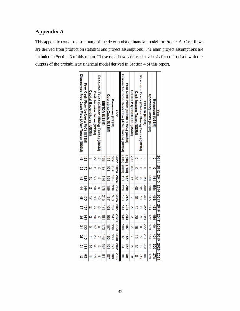
47
Appendix A
This appendix contains a summary of the deterministic financial model for Project A. Cash flows
are derived from production statistics and project assumptions. The main project assumptions are
included in Section 3 of this report. These cash flows are used as a basis for comparison with the
outputs of the probabilistic financial model derived in Section 4 of this report.
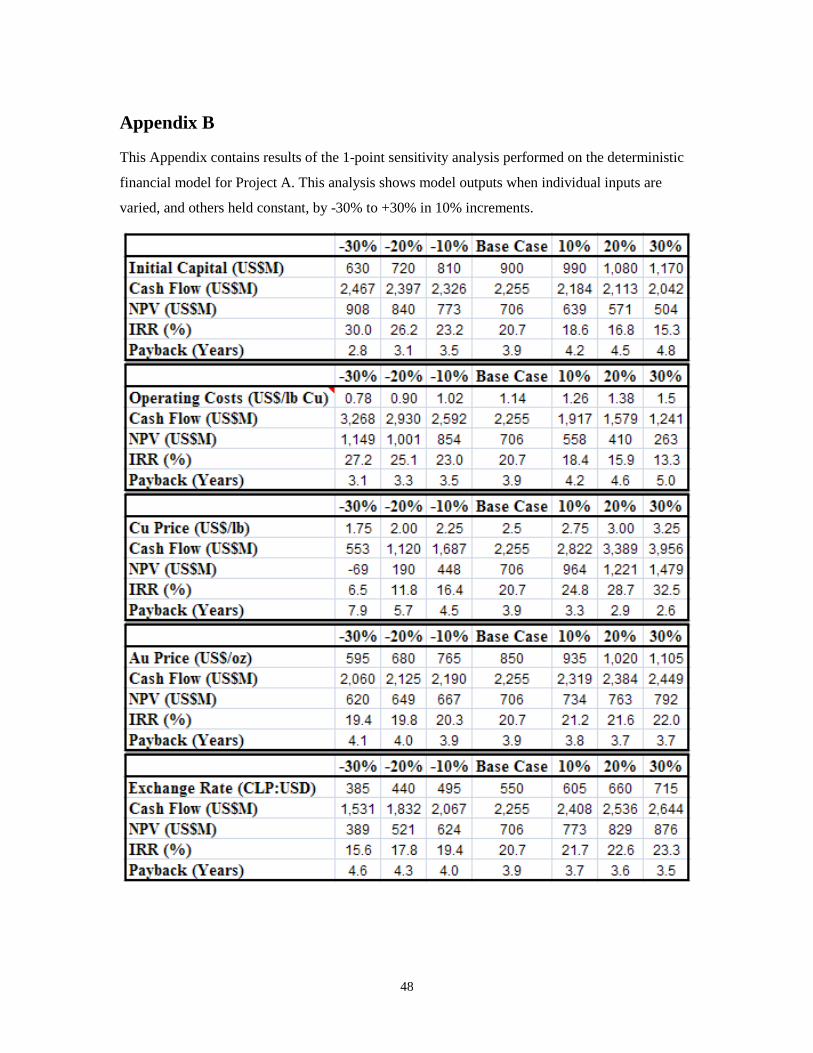
48
Appendix B
This Appendix contains results of the 1-point sensitivity analysis performed on the deterministic
financial model for Project A. This analysis shows model outputs when individual inputs are
varied, and others held constant, by -30% to +30% in 10% increments.
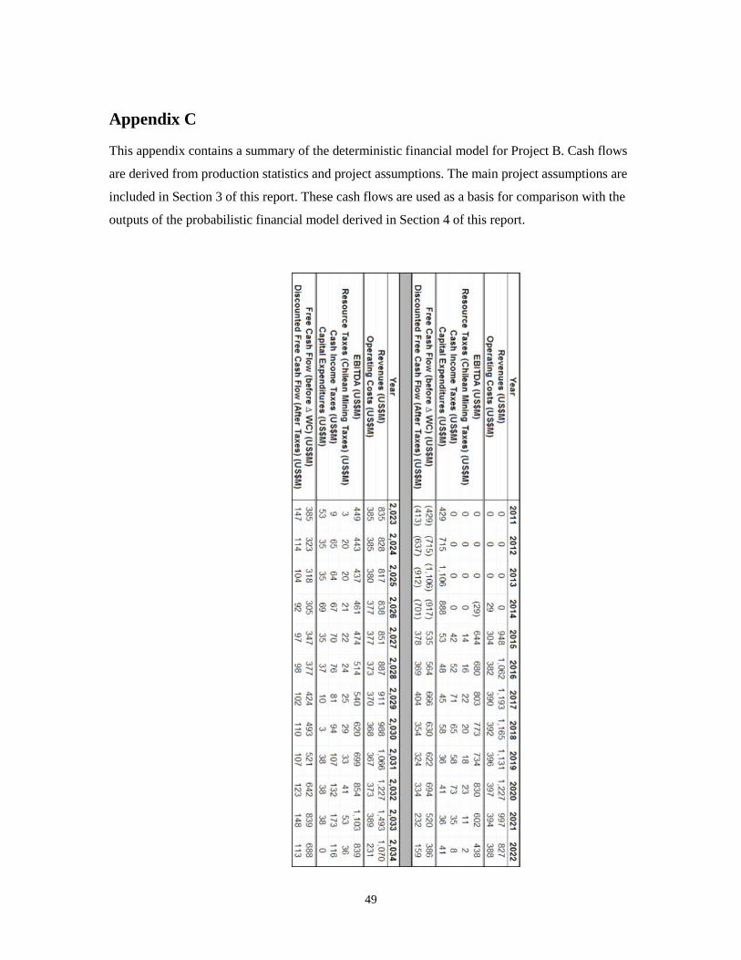
49
Appendix C
This appendix contains a summary of the deterministic financial model for Project B. Cash flows
are derived from production statistics and project assumptions. The main project assumptions are
included in Section 3 of this report. These cash flows are used as a basis for comparison with the
outputs of the probabilistic financial model derived in Section 4 of this report.
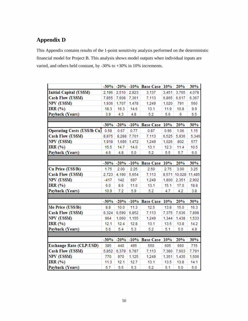
50
Appendix D
This Appendix contains results of the 1-point sensitivity analysis performed on the deterministic
financial model for Project B. This analysis shows model outputs when individual inputs are
varied, and others held constant, by -30% to +30% in 10% increments.
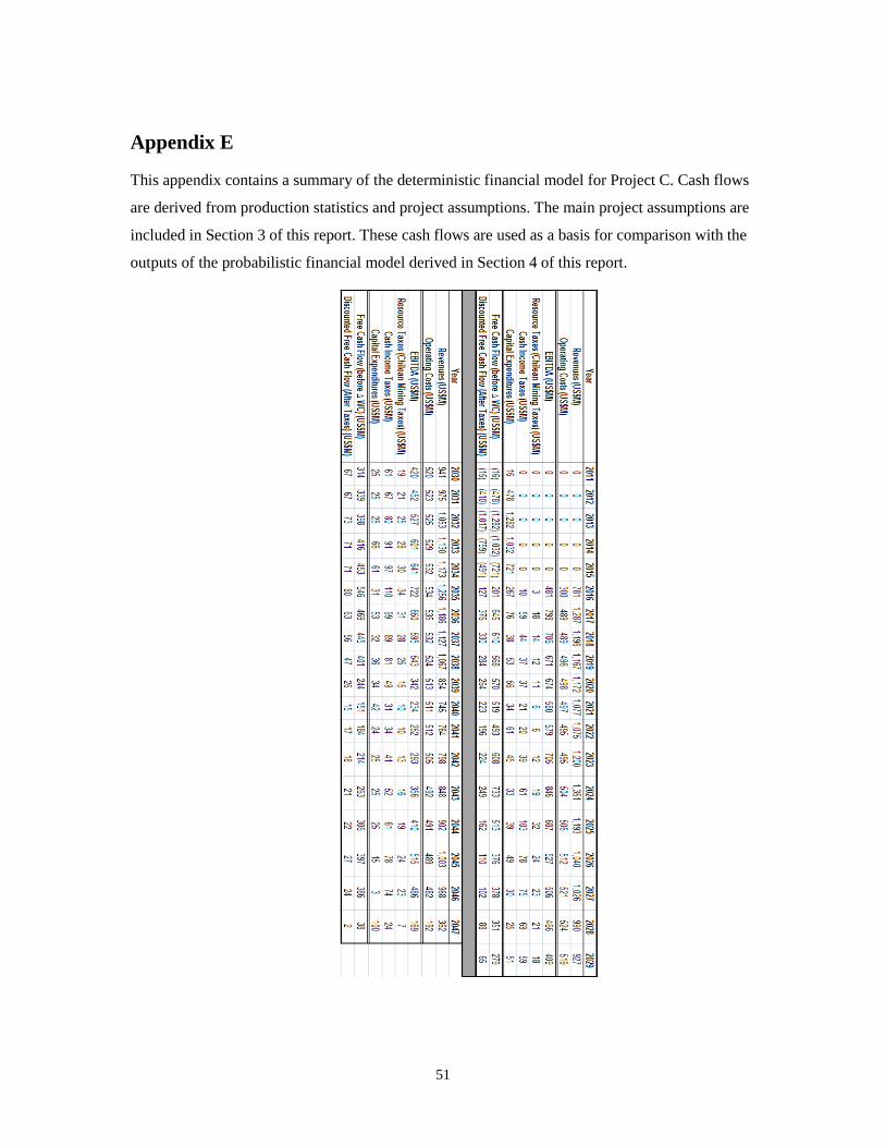
51
Appendix E
This appendix contains a summary of the deterministic financial model for Project C. Cash flows
are derived from production statistics and project assumptions. The main project assumptions are
included in Section 3 of this report. These cash flows are used as a basis for comparison with the
outputs of the probabilistic financial model derived in Section 4 of this report.
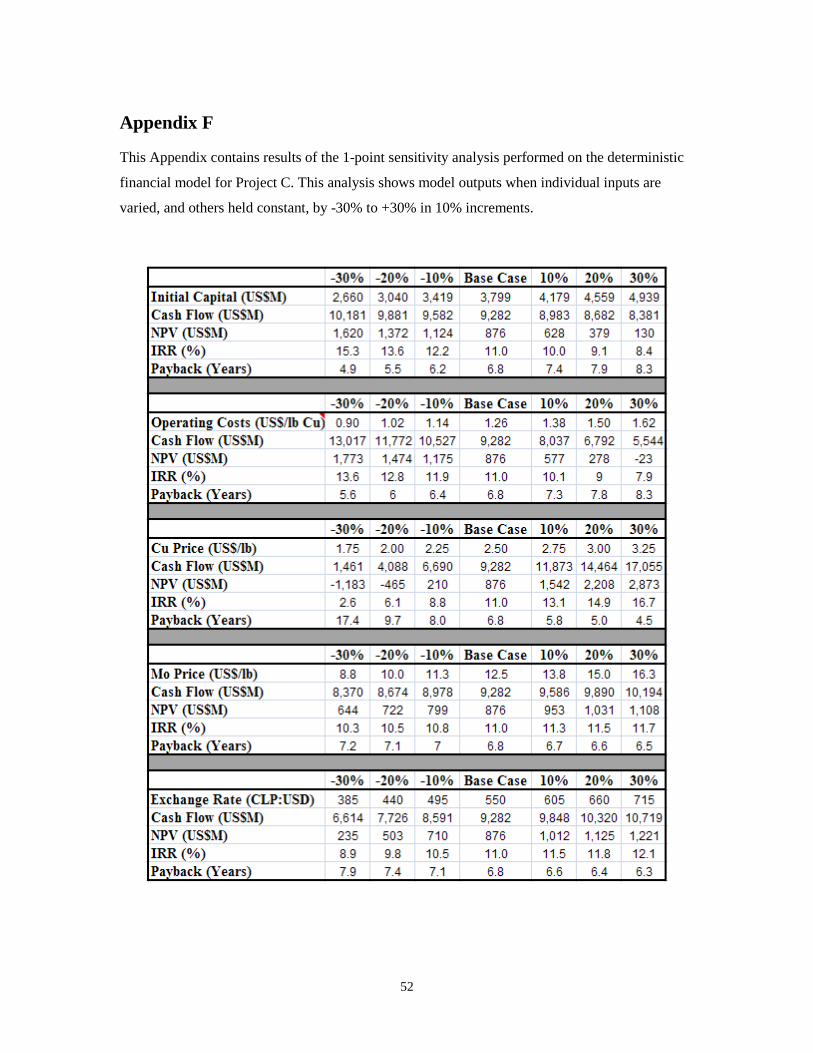
52
Appendix F
This Appendix contains results of the 1-point sensitivity analysis performed on the deterministic
financial model for Project C. This analysis shows model outputs when individual inputs are
varied, and others held constant, by -30% to +30% in 10% increments.
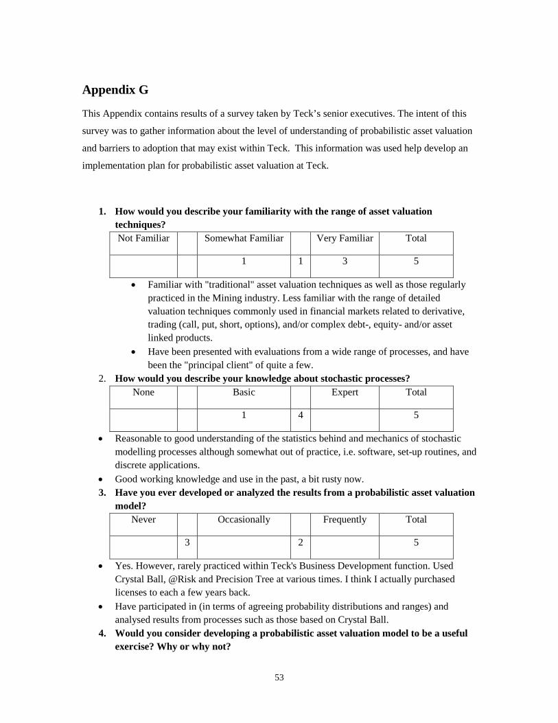
53
Appendix G
This Appendix contains results of a survey taken by Teck’s senior executives. The intent of this
survey was to gather information about the level of understanding of probabilistic asset valuation
and barriers to adoption that may exist within Teck. This information was used help develop an
implementation plan for probabilistic asset valuation at Teck.
1. How would you describe your familiarity with the range of asset valuation techniques?Not Familiar
Somewhat Familiar Very Familiar Total
1 1 3 5
• Familiar with "traditional" asset valuation techniques as well as those regularly practiced in the Mining industry. Less familiar with the range of detailed valuation techniques commonly used in financial markets related to derivative, trading (call, put, short, options), and/or complex debt-, equity- and/or asset linked products.
• Have been presented with evaluations from a wide range of processes, and have been the "principal client" of quite a few.
2. None
How would you describe your knowledge about stochastic processes? Basic Expert Total
1 4 5
• Reasonable to good understanding of the statistics behind and mechanics of stochastic modelling processes although somewhat out of practice, i.e. software, set-up routines, and discrete applications.
• Good working knowledge and use in the past, a bit rusty now. 3.
Never
Have you ever developed or analyzed the results from a probabilistic asset valuation model?
Occasionally Frequently Total
3 2 5
• Yes. However, rarely practiced within Teck's Business Development function. Used Crystal Ball, @Risk and Precision Tree at various times. I think I actually purchased licenses to each a few years back.
• Have participated in (in terms of agreeing probability distributions and ranges) and analysed results from processes such as those based on Crystal Ball.
4. Would you consider developing a probabilistic asset valuation model to be a useful exercise? Why or why not?
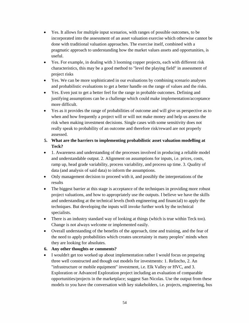
54
• Yes. It allows for multiple input scenarios, with ranges of possible outcomes, to be incorporated into the assessment of an asset valuation exercise which otherwise cannot be done with traditional valuation approaches. The exercise itself, combined with a pragmatic approach to understanding how the market values assets and opportunities, is useful.
• Yes. For example, in dealing with 3 looming copper projects, each with different risk characteristics, this may be a good method to "level the playing field" in assessment of project risks
• Yes. We can be more sophisticated in our evaluations by combining scenario analyses and probabilistic evaluations to get a better handle on the range of values and the risks.
• Yes. Even just to get a better feel for the range in probable outcomes. Defining and justifying assumptions can be a challenge which could make implementation/acceptance more difficult.
• Yes as it provides the range of probabilities of outcome and will give us perspective as to when and how frequently a project will or will not make money and help us assess the risk when making investment decisions. Single cases with some sensitivity does not really speak to probability of an outcome and therefore risk/reward are not properly assessed.
5.
• 1. Awareness and understanding of the processes involved in producing a reliable model and understandable output. 2. Alignment on assumptions for inputs, i.e. prices, costs, ramp up, head grade variability, process variability, and process up time. 3. Quality of data (and analysis of said data) to inform the assumptions.
What are the barriers to implementing probabilistic asset valuation modelling at Teck?
• Only management decision to proceed with it, and possibly the interpretations of the results
• The biggest barrier at this stage is acceptance of the techniques in providing more robust project valuations, and how to appropriately use the outputs. I believe we have the skills and understanding at the technical levels (both engineering and financial) to apply the techniques. But developing the inputs will invoke further work by the technical specialists.
• There is an industry standard way of looking at things (which is true within Teck too). Change is not always welcome or implemented easily.
• Overall understanding of the benefits of the approach, time and training, and the fear of the need to apply probabilities which creates uncertainty in many peoples’ minds when they are looking for absolutes.
6. • I wouldn't get too worked up about implementation rather I would focus on preparing
three well constructed and though out models for investments: 1. Relincho, 2. An "infrastructure or mobile equipment" investment, i.e. Elk Valley or HVC, and 3. Exploration or Advanced Exploration project including an evaluation of comparable opportunities/projects in the marketplace; suggest San Nicolas. Use the output from these models to you have the conversation with key stakeholders, i.e. projects, engineering, bus
Any other thoughts or comments?

55
dev, and finance, about how to use stochastic modelling approach to valuation, and then steps to implement more regularly. • These techniques are being more widely adopted, and as a minimum Teck needs to keep up. Over analysis is quite possible, so an early step is to developing a broad understanding of the purpose and value of using these techniques.
56
Reference List
Andersson, K. (2007). Are commodity prices mean reverting? Applied Financial Economics, 17,
781.
Bedford, T., & Cooke, R. (2001). Probabilistic Risk Analysis. Cambridge: Cambridge University
Press, 3.
Bernard, J.T., Khalaf, L., Kichian, M., & Mcmahon, S. (2008). Forecasting commodity prices:
GARCH, Jumps, and Mean Reversion. Journal of Forecasting, 27, 289.
Bier, V.M. (1999). Challenges to the acceptance of probabilistic risk analysis. Risk Analysis,
19(4), 705-706.
Bloomberg Finance L.P. (2011). LME copper spot prices and Chilean peso exchange rates from
01/01/02 to 01/14/11. from Bloomberg Professional database.
Dixit, A.K., & Pindyck, R.S. (1994). Investment under uncertainty. Princeton, New Jersey:
Princeton University Press, 60-78.
57
Graham, J.R., & Harvey, C.R. (2001). The theory and practice of corporate finance: Evidence
from the field. Journal of Financial Economics, 60, 6.
Hertz, D.B. (1964). Risk Analysis in Capital Investment. Harvard Business Review, 95-106.
Ho, S.S.M., & Pike, R.H. (1992). Adoption of probabilistic risk analysis in capital budgeting and
corporate investment. Journal of Business & Accounting, 19(3), 390-399.
Hull, J.C. (1980). The Evaluation of Risk in Business Investment. Oxford: Pergamon Press.
Ivanhoe Mines Ltd. (June 2010). Oyu Tolgoil Technical Report (NI 43-101). Retrieved from
SEDAR.
Kotter, J., & Cohen, D. (2002). The Heart of Change. Boston, Massachusetts: Harvard Business
School Press.
Laughton, D. (2007). The Banff Taxonomy of Asset Valuation Methods: Lessons from Financial
Markets for Real Asset Valuation in the Upstream Petroleum Industry, 2.
Neuhauser, J.J, & Viscione, J.A. (1973). How managers feel about advanced capital budgeting
methods. Management Review, 21.

58
Samis, M., & Davis, G (2007). Using Dynamic DCF and Real Options to Value and Manage
Natural Resource Projects. AMEC Americas Limited & The Colorado School of Mines,
D2M.8-10.
Schwartz, E.S. (1997). The stochastic behavior of commodity prices: Implications for valuation
and hedging. The Journal of Finance, 52(3), 926.
Uhlenbeck, G.E., & Ornstein, L.S. (1930). On the theory of Brownian motion. Physical Review,
36(5), 823.


![ASSET Valuation[1]](https://img.pdfslide.us/doc/110x75/577d27af1a28ab4e1ea48bd2/asset-valuation1.jpg)