Embed Size (px)
Citation preview
Privacy-Friendly Mobility Analytics usingAggregate Location Data
Apostolos PyrgelisUniversity College London
Emiliano De CristofaroUniversity College [email protected]
Gordon J. RossUniversity College London
ABSTRACTLocation data can be extremely useful to study commuting pat-
terns and disruptions, as well as to predict real-time traffic volumes.At the same time, however, the fine-grained collection of user lo-cations raises serious privacy concerns, as this can reveal sensitiveinformation about the users, such as, life style, political and reli-gious inclinations, or even identities. In this paper, we study thefeasibility of crowd-sourced mobility analytics over aggregate lo-cation information: users periodically report their location, usinga privacy-preserving aggregation protocol, so that the server canonly recover aggregates – i.e., how many, but not which, users arein a region at a given time. We experiment with real-world mobil-ity datasets obtained from the Transport For London authority andthe San Francisco Cabs network, and present a novel methodol-ogy based on time series modeling that is geared to forecast trafficvolumes in regions of interest and to detect mobility anomalies inthem. In the presence of anomalies, we also make enhanced trafficvolume predictions by feeding our model with additional informa-tion from correlated regions. Finally, we present and evaluate a mo-bile app prototype, called Mobility Data Donors (MDD), in termsof computation, communication, and energy overhead, demonstrat-ing the real-world deployability of our techniques.
1. INTRODUCTIONThe availability of information about people’s locations and
movements holds the promise to make urban planning more ef-fective and efficient, and ultimately improve citizens’ quality oflife. Prompted by the increased presence of always-on, always-connected devices, the ubiquitous collection of location informa-tion enables a number of interesting applications. New researchfrontiers, e.g., in the field of anticipatory mobile computing, makeit increasingly possible to use mobile sensing along with machinelearning for intelligent reasoning [32]. For instance, contextual lo-cation information collected from mobile users can be used to pre-dict future mobility events [26, 39], detect mobility anomalies [30]and enable real-time traffic or event statistics [4].
At the same time, however, large-scale collection of individualusers’ fine-grained locations raises serious privacy concerns, as thiscan reveal sensitive information about the users, such as, life style,political and religious inclinations, or even identities [31, 24]. Al-though often advocated, anonymization of location traces is mootas these reveal home/work locations, which in turn can be used tore-identify users [18]. In fact, just a few locations are enough tore-identify users [43]. Therefore, in this paper, we set to investigatewhether or not mobility analytics can be effectively and efficientlyperformed over aggregate data. We turn to cryptographic proto-cols for privacy-friendly data aggregation and use them to privatelygather location statistics [9, 23, 28, 34]. Overall, we aim to demon-
strate: (1) the usefulness of mobility analytics over aggregate loca-tions, and (2) the real-world deployability of a scalable system forprivacy-friendly location data collection.Roadmap. We present a crowd-sourced system for privacy-friendly mobility analytics whereby users periodically report lo-cations, but do so using a privacy-preserving aggregation protocol,so that only aggregates can be recovered (i.e., how many but notwhich users were in a region at a given time). We experiment withreal-world mobility datasets obtained from the Transport For Lon-don (TFL) authority as well as the San Francisco Cabs (SFC) net-work, and present a methodology based on time series modelinggeared to forecast traffic volumes in regions of interest (ROIs) andto detect mobility anomalies in them. In the presence of anomalies,we also make enhanced traffic volume predictions (achieving upto 50% improvement) by training our model with additional infor-mation from correlated regions. Such tasks are particularly usefulin modern cities for journey planning [4, 26] and congestion pre-vention [38]. Finally, we show how to build a privacy-respectingsystem for data collection. To this end, we present a mobile appprototype, called Mobility Data Donors (MDD), and present anempirical evaluation of its computation, communication, and en-ergy complexities, which attest to the practicality of our vision.Paper Organization. Next section introduces a few concepts andtools used in our work, then, Section 3 presents our datasets andour methodology for predictive mobility analytics. In Section 4, wediscuss the details of our proposed framework and analyze its real-world deployment. Finally, after reviewing related work in Sec-tion 5, the paper concludes in Section 6.
2. PRELIMINARIES
2.1 Auto Regressive Moving AverageAs we aim to perform analytics on aggregate locations – specif-
ically, predicting traffic volumes as well as detecting mobilityanomalies in a Region Of Interest (ROI), such as underground sta-tions (cf. Section 3.2–3.3) – we model ROIs’ time series usingAuto-Regressive Moving Average (ARMA). We build on the workby Box et al. [8], who present an iterative method for choosing andestimating ARMA models.
Given a time series Yt, an ARMA model is a tool for under-standing and predicting future values in Yt. The model is usuallydenoted asARMA(p, q), whereAR(p) denotes the autoregressivemodel of order p and MA(q) refers to the moving average modelof order q. Specifically, an ARMA(p, q) model is defined as:
Yt = c+
p∑i=1
φi · Yt−i + εt +
q∑i=1
θi · εt−i (1)
arX
iv:1
609.
0658
2v2
[cs
.CR
] 9
Oct
201
6
where c is a constant, φ1, . . . , φp and θ1, . . . , θq are model param-eters, and εt, εt−1, . . . are white noise error terms.
2.2 Vector Auto-RegressionWe also investigate how to improve traffic volume predictions in
the presence of anomalies (cf. Section 3.4), thus, we also attempt todiscover correlated ROIs and use their aggregate time series, alongwith a Vector Auto-Regression (VAR) model, to make enhancedpredictions. VARs are statistical models used in econometrics tocapture linear interdependencies among multiple time series, andconsist a generalization of uni-variate autoregressive models (ARmodels) that allow more than one evolving variable. All variablesin a VAR model are treated symmetrically and each of them hasan equation explaining its evolution based on its own lags as wellas those of the other model variables. VAR modeling requires theprior knowledge of a list of variables which can be hypothesized toaffect each other inter-temporally.
A VAR model describes the evolution of a set of k variables (en-dogenous variables) over a sample period t = 1, . . . , T as a linearfunction of their past values. The variables are collected in a vectoryt of size (k, 1), whose ith element yit is the observation of thevariable i at time t. A p-th order VAR model, denoted as V AR(p)is given by the equation:
yt = c+A1 · yt−1 +A2 · yt−2 + . . . Ap · yt−p + et (2)
where c is a vector of constants with size (k, 1), Ai is a time-invariant matrix of size (k, k) and et is a vector of error terms withsize (k, 1) where: (a) E(et) = 0, every error term has mean zero,(b)E(ete
′t) = Ω, the co-variance matrix of error terms is Ω and (c)
E(ete′t−k) = 0, for any non-zero k there is no serial correlation in
individual error terms.
2.3 Spearman CorrelationTo discover correlated ROIs, we will use Spearman’s correlation
coefficient, which is a non-parametric measure of the statistical de-pendence between the ranking of two variables [12]. It provides anestimate of how well the relationship between two variables can bedescribed with a monotonic function and, unlike Pearson, it doesnot assume that both variables are normally distributed. Given twovariables W,Z, the Spearman correlation coefficient is defined as:
rs = 1− 6 ·∑d2i
n · (n2 − 1)(3)
where di = rg(Wi) − rg(Zi) is the difference between the tworanks of each observation and n is the number of observations.Similar to other correlation measures, Spearman’s obtains valuesbetween −1 and +1, with 0 implying no correlation, and −1 or+1 implying an exact monotonic relationship. Intuitively, positivecorrelations imply that as W increases, so does Z, while negativecorrelations mean that as W increases, Z decreases.
2.4 Privacy-Preserving Data AggregationWe also use cryptographic protocols for privacy-preserving data
aggregation, allowing an untrusted aggregator to gather statistics(e.g., sum or mean) from users in such a way that data of singleusers is not revealed in the clear, but only the aggregate informationcan be recovered. These protocols are often used for smart meter-ing [25], participatory sensing [34], or recommender systems [28].
Typically, private aggregation relies on a cryptosystem that is ad-ditively homomorphic: users send encrypted data to the aggregator,which does not hold the corresponding decryption key and cannotaccess single users’ contributions, however, it can decrypt the sumof all users’ reports. Specifically, we choose a protocol recently
proposed by Melis et al. [28], as it guarantees: scalability, indepen-dence from trusted third parties and/or key distribution centers, andfault tolerance. Scalability is achieved by combining the private ag-gregation protocol of Kursawe et al. [25] (secure under the Compu-tational Diffie Hellman assumption in the presence of honest-but-curious adversaries) with data structures supporting succinct datarepresentation, i.e., Count-Min Sketches [13]. These introduce asmall, upper-bounded error in the aggregation, but reduce the com-putational/communication complexities of the cryptographic oper-ations from linear to logarithmic in the size of the input. It alsofeatures a completely distributed key generation/distribution which,unlike other protocols, e.g. [22, 34], does not require any other au-thorities. Finally, its fault tolerance protocol addresses one of themain limitations of [25], i.e., if one or more users fails to reporttheir (encrypted) data, the aggregator cannot correctly decrypt theaggregate (since it relies on encryption keys summing up to zero).
Melis et al. [28]’s protocol consists of four phases. (1) Setup:Assuming a cyclic group G of order q for which the Computa-tional Diffie-Hellman problem is hard, and g a generator of thisgroup, each user Ui ∈ U = 1, . . . , N generates a private keyxi ∈r G (i.e., sampled at random from G) and a public keyyi = gxi mod q. The public keys are published with the aggre-gator. (2) Encryption: Each user Ui holds an input vector of datapoints S = Sc ∈ N, c = 1, . . . , T. To participate in theprivacy-preserving aggregation each user needs to generate blind-ing factors based on the public keys of the other users in such away that they all sum up to zero. At round s, for l = 1, . . . , T ,user Ui computes kil =
∑Nj=1,j 6=iH(yxi
j ‖l‖s) · (−1)i>j mod q,where H is a cryptographic hash function and ‖ denotes the con-catenation operator. Then, for each entry SilTl=1, Ui encryptsSil as bil = Sil + kilmod 232 and sends the resulting ciphertextto the aggregator. (3) Aggregation: The aggregator collects theciphertexts from each user Ui and (obliviously) aggregates them.More precisely, for l = 1, . . . , T it computes Cl =
∑Ni=1 bil =∑N
i=1 kil +∑N
i=1 Sil =∑N
i=1 Silmod 232, where Cl denotes thel− th item of the input vector S. (4) Fault Recovery: If, during theaggregation phase, only a subset of users Uon successfully submitdata, the aggregator sends Uon to each Ui ∈ Uon and Ui com-putes, for each l = 1, . . . , T , k
′il =
∑Nj=1,j 6=i,j /∈Uon
H(yxij ‖l‖s) ·
(−1)i>j mod q. Then each user Ui sends these values back to tothe aggregator who can now obtain the aggregate counts by com-puting C
′l = (
∑i∈Uon
bil −∑
i∈Uonk
′il)mod 232.
Groups. Another feature of [28] is the ability to dynamically al-locate users in groups, and perform within-group aggregation andthen combining statistics from multiple groups, which is crucialto cope with dynamic/mobile settings. It also allows to bound thecomplexity of the encryption phase, which depends on the numberof users in the group.
Input Compression. As mentioned above, [28] uses Count-MinSketches to guarantee scalability when the input vector (S) is large.Specifically, the encryption phase is modified as follows: each userUi initializes a Count-Min Sketch vector Xi ∈ Nd×w with zeroentries, then encodes his original input vector S using the updateprocedure of Count-Min Sketches [13] while employing the fol-lowing pairwise hash function: h(x) = ((a ·x+ b)mod p)modwfor a 6= 0, b random integers modulo a random prime p. Then eachuser encrypts Xi as in the previously described encryption phase.
If |S| denotes the size of the input vector S, its compact represen-tation with a Count-Min Sketch has size O(log(|S|)). More pre-cisely, given the sketch parameters (ε, δ), the Count-Min Sketch isa vector of sizeL = d×w where d = dln (|S|/δ)e andw = de/εe.For instance, if ε = δ = 0.01, a vector S of size |S| = 104 can
be encoded as a sketch of size L = 3, 808, while a vector S of size|S| = 106 can be represented as a sketch of size L = 5, 168. Ob-viously, the Count-Min succinct structure introduces an accuracyerror and its parameters (ε, δ) give an upper bounded error for theestimated counters ci, amounting to ci ≤ ci + ε ·
∑j |cj | with
probability 1− δ (with ci being the true element of the vector).
3. MOBILITY ANALYTICS USINGAGGREGATE LOCATIONS
We now present and evaluate our “mobility analytics” algo-rithms, specifically, predicting traffic volumes at ROIs, discoveringand predicting anomalies – all using aggregate location reports. Werely on two real-world datasets obtained, respectively, from Trans-port for London (TFL) and the San Francisco Cab (SFC) network.
3.1 Datasets
3.1.1 Transport For London (TFL)London’s transportation system consists of various connected
subsystems: London Underground Ltd (LUL), London TransportBuses (LTB), Docklands Light Rail (DLR), Overground (LRC),Tramlink (TRAM), and National Rail (NR), operating in the cityunder the umbrella of Transport for London (TFL). The most com-mon payment method for TFL fares is the Oyster Card, a pre-paid,RFID-enabled card. We have obtained from TFL data correspond-ing to all March 2010 trips from all (anonymized) oyster cards,which we pre-process in the following way. First, we discard tripsfrom TRAM due to scarce density and LTB for consistency as trav-elers only tap-in but do not tap-out for bus trips paid by Oyster.Then, to observe weekly patterns, we focus on the four weeks fromMonday March 1 to Sunday 28, 2010. The final dataset consistsof approximately 60 million oyster-card trips, performed by almost4 million unique users, over 582 stations. Each entry in the datadescribes a unique trip and consists of the following fields: oysterid, start time, start station id, end time, and end station id. Notethat the time resolution of the timestamps is 1 minute.
Next, we aggregate single-trip records by grouping trips start andend times in time epochs of 1 hour, aiming to achieve regularity intransit patterns (similar to [45]), and count the number of passen-gers that entered (“tap-in”) or exited (“tap-out”) each station duringa slot. For each station i ∈ 1, . . . , n (with n being the total num-ber of stations), we create a time series Yit indicating how manypassengers transited through it in a time epoch t ∈ 1, . . . ,m (mdenotes the total number of epochs, i.e., 672): Yit = Y in
it + Y outit ,
where Y init indicates the number of tap-in events and Y out
it the num-ber of tap-out events, at station i during epoch t.
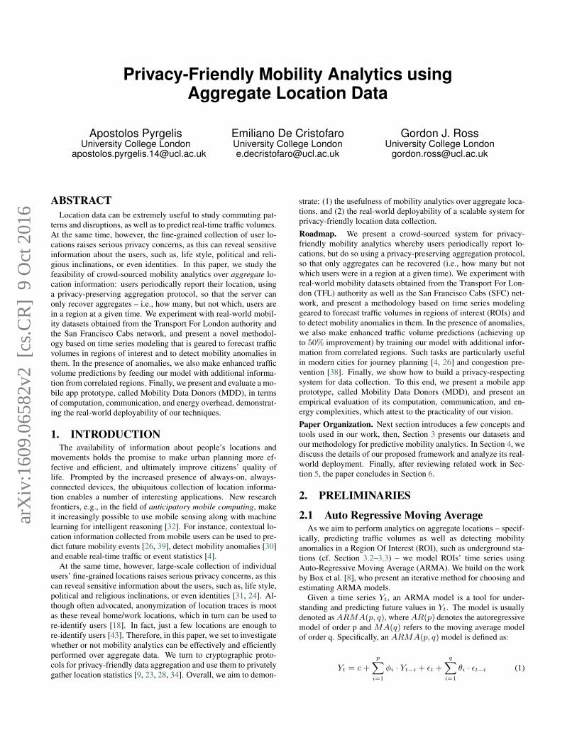
In Figure 1, we plot the hourly aggregate time series of two sta-tions – Canary Wharf (one of the busiest stations of London) andClapham Common (a moderately busy station) – showing differentpatterns during weekdays and weekends, as well as peak commut-ing hours. In general, we note some weekly/daily seasonality in thestations’ time series as well as stationarity (i.e., no particular trend).We verify the latter by performing the Augmented Dickey-Fullertest [14] which indicates that 93% of tube stations have stationarytime series with 95% confidence.
3.1.2 San Francisco Cab (SFC)We also use the San Francisco Cab (SFC) dataset [33], which
contains mobility traces recorded by taxis in San Francisco, be-tween May 17 to June 10, 2008. The dataset contains approxi-mately 11 million GPS coordinates, generated by 536 taxis. Toobserve weekly patterns in our data we sample the dataset to cover
(a)
(b)
Figure 1: Hourly traffic volume at two TFL stations (March 1–28, 2010).
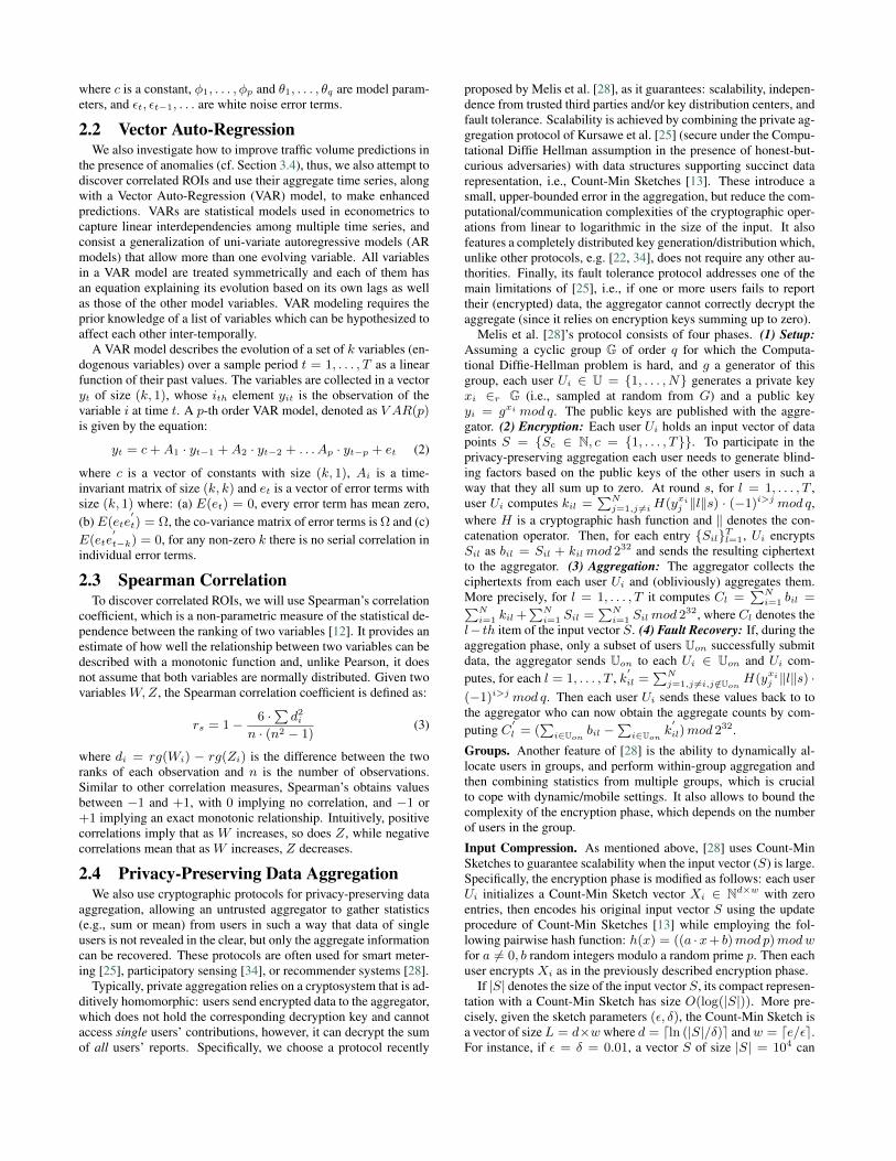
Figure 2: Number of cabs on 100× 100 SF grid (May 19 – June 8, 2008).
exactly 3 weeks of data: Monday May 19 to Sunday June 8, 2008.Entries in the dataset include the following fields: cab identifier,latitude, longitude and a time stamp in UNIX epoch format.
We follow a similar approach as with the TFL dataset to ag-gregate the traces, however, since locations are GPS coordinatesrather than points of interest, we divide the city of San Franciscointo a grid S consisting of 100 × 100 regions, each covering anarea of 0.19 × 0.14 square miles. We group the GPS traces inone-hour epochs and, for each region i ∈ 1, . . . , n (with n be-ing the total number of regions, i.e., 10,000), we count the numberof taxis that have reported a presence in that block during epocht ∈ 1, . . . ,m (m being the number of time epochs, i.e., 504),and create a time series Yit as: Yit =
∑kj=1 pjt, where k is the
total number of taxis (i.e., 536) and pjt ∈ 0, 1 indicates whethertaxi j ∈ 1, . . . , k reported its location at region i during epoch t.
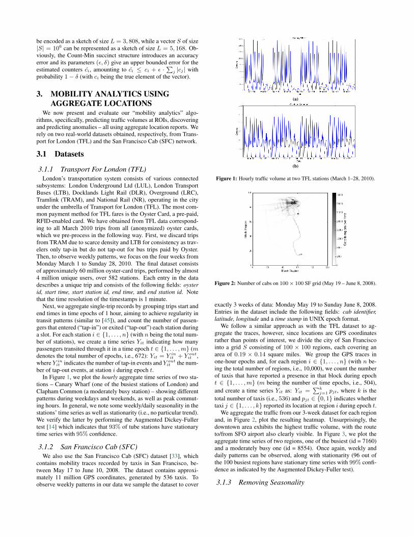
We aggregate the traffic from our 3-week dataset for each regionand, in Figure 2, plot the resulting heatmap. Unsurprisingly, thedowntown area exhibits the highest traffic volume, with the routeto/from SFO airport also clearly visible. In Figure 3, we plot theaggregate time series of two regions, one of the busiest (id = 7160)and a moderately busy one (id = 8554). Once again, weekly anddaily patterns can be observed, along with stationarity (96 out ofthe 100 busiest regions have stationary time series with 99% confi-dence as indicated by the Augmented Dickey-Fuller test).
3.1.3 Removing Seasonality
(a)
(b)
Figure 3: Hourly traffic volume in regions 7160 and 8554 of SFC dataset.
Our preliminary analysis of both datasets shows that aggregatetime series of the ROIs (tube stations or regions) exhibit no partic-ular trend but do preserve weekly/daily seasonality. Therefore, asproposed in prior work, e.g., [21], we de-seasonalize each region’stime series via additive decomposition. More specifically:
Dit = Yit − Yit (4)
where Yit is the ROI’s original time series i and Yit is its sea-sonality defined as Yit = 1
w
∑Yidh, with w being the num-
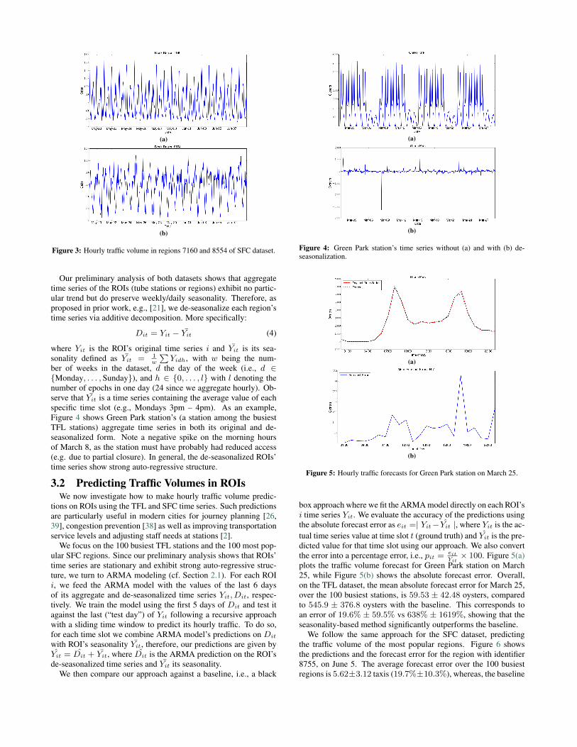
ber of weeks in the dataset, d the day of the week (i.e., d ∈Monday, . . . , Sunday), and h ∈ 0, . . . , l with l denoting thenumber of epochs in one day (24 since we aggregate hourly). Ob-serve that Yit is a time series containing the average value of eachspecific time slot (e.g., Mondays 3pm – 4pm). As an example,Figure 4 shows Green Park station’s (a station among the busiestTFL stations) aggregate time series in both its original and de-seasonalized form. Note a negative spike on the morning hoursof March 8, as the station must have probably had reduced access(e.g. due to partial closure). In general, the de-seasonalized ROIs’time series show strong auto-regressive structure.
3.2 Predicting Traffic Volumes in ROIsWe now investigate how to make hourly traffic volume predic-
tions on ROIs using the TFL and SFC time series. Such predictionsare particularly useful in modern cities for journey planning [26,39], congestion prevention [38] as well as improving transportationservice levels and adjusting staff needs at stations [2].
We focus on the 100 busiest TFL stations and the 100 most pop-ular SFC regions. Since our preliminary analysis shows that ROIs’time series are stationary and exhibit strong auto-regressive struc-ture, we turn to ARMA modeling (cf. Section 2.1). For each ROIi, we feed the ARMA model with the values of the last 6 daysof its aggregate and de-seasonalized time series Yit, Dit, respec-tively. We train the model using the first 5 days of Dit and test itagainst the last (“test day”) of Yit following a recursive approachwith a sliding time window to predict its hourly traffic. To do so,for each time slot we combine ARMA model’s predictions on Dit
with ROI’s seasonality Yit, therefore, our predictions are given byYit = Dit + Yit, where Dit is the ARMA prediction on the ROI’sde-seasonalized time series and Yit its seasonality.
We then compare our approach against a baseline, i.e., a black
(a)
(b)
Figure 4: Green Park station’s time series without (a) and with (b) de-seasonalization.
(a)
(b)
Figure 5: Hourly traffic forecasts for Green Park station on March 25.
box approach where we fit the ARMA model directly on each ROI’si time series Yit. We evaluate the accuracy of the predictions usingthe absolute forecast error as eit =| Yit− Yit |, where Yit is the ac-tual time series value at time slot t (ground truth) and Yit is the pre-dicted value for that time slot using our approach. We also convertthe error into a percentage error, i.e., pit = eit
Yit× 100. Figure 5(a)
plots the traffic volume forecast for Green Park station on March25, while Figure 5(b) shows the absolute forecast error. Overall,on the TFL dataset, the mean absolute forecast error for March 25,over the 100 busiest stations, is 59.53 ± 42.48 oysters, comparedto 545.9 ± 376.8 oysters with the baseline. This corresponds toan error of 19.6% ± 59.5% vs 638% ± 1619%, showing that theseasonality-based method significantly outperforms the baseline.
We follow the same approach for the SFC dataset, predictingthe traffic volume of the most popular regions. Figure 6 showsthe predictions and the forecast error for the region with identifier8755, on June 5. The average forecast error over the 100 busiestregions is 5.62±3.12 taxis (19.7%±10.3%), whereas, the baseline
(a)
(b)
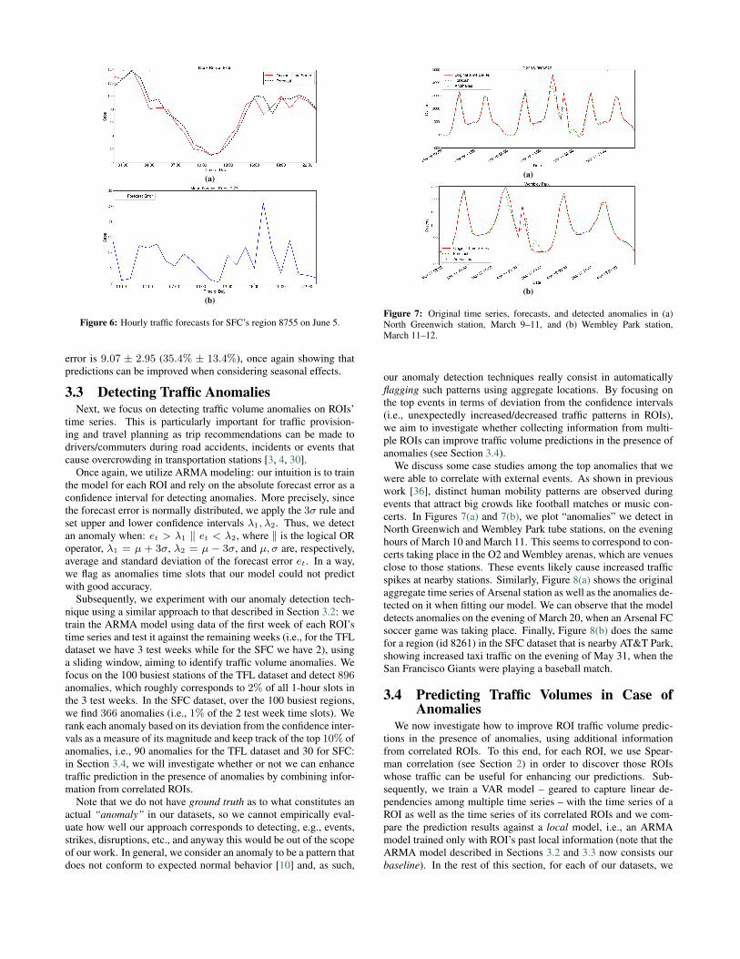
Figure 6: Hourly traffic forecasts for SFC’s region 8755 on June 5.
error is 9.07 ± 2.95 (35.4% ± 13.4%), once again showing thatpredictions can be improved when considering seasonal effects.
3.3 Detecting Traffic AnomaliesNext, we focus on detecting traffic volume anomalies on ROIs’
time series. This is particularly important for traffic provision-ing and travel planning as trip recommendations can be made todrivers/commuters during road accidents, incidents or events thatcause overcrowding in transportation stations [3, 4, 30].
Once again, we utilize ARMA modeling: our intuition is to trainthe model for each ROI and rely on the absolute forecast error as aconfidence interval for detecting anomalies. More precisely, sincethe forecast error is normally distributed, we apply the 3σ rule andset upper and lower confidence intervals λ1, λ2. Thus, we detectan anomaly when: et > λ1 ‖ et < λ2, where ‖ is the logical ORoperator, λ1 = µ + 3σ, λ2 = µ − 3σ, and µ, σ are, respectively,average and standard deviation of the forecast error et. In a way,we flag as anomalies time slots that our model could not predictwith good accuracy.
Subsequently, we experiment with our anomaly detection tech-nique using a similar approach to that described in Section 3.2: wetrain the ARMA model using data of the first week of each ROI’stime series and test it against the remaining weeks (i.e., for the TFLdataset we have 3 test weeks while for the SFC we have 2), usinga sliding window, aiming to identify traffic volume anomalies. Wefocus on the 100 busiest stations of the TFL dataset and detect 896anomalies, which roughly corresponds to 2% of all 1-hour slots inthe 3 test weeks. In the SFC dataset, over the 100 busiest regions,we find 366 anomalies (i.e., 1% of the 2 test week time slots). Werank each anomaly based on its deviation from the confidence inter-vals as a measure of its magnitude and keep track of the top 10% ofanomalies, i.e., 90 anomalies for the TFL dataset and 30 for SFC:in Section 3.4, we will investigate whether or not we can enhancetraffic prediction in the presence of anomalies by combining infor-mation from correlated ROIs.
Note that we do not have ground truth as to what constitutes anactual “anomaly” in our datasets, so we cannot empirically eval-uate how well our approach corresponds to detecting, e.g., events,strikes, disruptions, etc., and anyway this would be out of the scopeof our work. In general, we consider an anomaly to be a pattern thatdoes not conform to expected normal behavior [10] and, as such,
(a)
(b)
Figure 7: Original time series, forecasts, and detected anomalies in (a)North Greenwich station, March 9–11, and (b) Wembley Park station,March 11–12.
our anomaly detection techniques really consist in automaticallyflagging such patterns using aggregate locations. By focusing onthe top events in terms of deviation from the confidence intervals(i.e., unexpectedly increased/decreased traffic patterns in ROIs),we aim to investigate whether collecting information from multi-ple ROIs can improve traffic volume predictions in the presence ofanomalies (see Section 3.4).
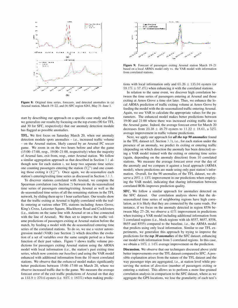
We discuss some case studies among the top anomalies that wewere able to correlate with external events. As shown in previouswork [36], distinct human mobility patterns are observed duringevents that attract big crowds like football matches or music con-certs. In Figures 7(a) and 7(b), we plot “anomalies” we detect inNorth Greenwich and Wembley Park tube stations, on the eveninghours of March 10 and March 11. This seems to correspond to con-certs taking place in the O2 and Wembley arenas, which are venuesclose to those stations. These events likely cause increased trafficspikes at nearby stations. Similarly, Figure 8(a) shows the originalaggregate time series of Arsenal station as well as the anomalies de-tected on it when fitting our model. We can observe that the modeldetects anomalies on the evening of March 20, when an Arsenal FCsoccer game was taking place. Finally, Figure 8(b) does the samefor a region (id 8261) in the SFC dataset that is nearby AT&T Park,showing increased taxi traffic on the evening of May 31, when theSan Francisco Giants were playing a baseball match.
3.4 Predicting Traffic Volumes in Case ofAnomalies
We now investigate how to improve ROI traffic volume predic-tions in the presence of anomalies, using additional informationfrom correlated ROIs. To this end, for each ROI, we use Spear-man correlation (see Section 2) in order to discover those ROIswhose traffic can be useful for enhancing our predictions. Sub-sequently, we train a VAR model – geared to capture linear de-pendencies among multiple time series – with the time series of aROI as well as the time series of its correlated ROIs and we com-pare the prediction results against a local model, i.e., an ARMAmodel trained only with ROI’s past local information (note that theARMA model described in Sections 3.2 and 3.3 now consists ourbaseline). In the rest of this section, for each of our datasets, we
(a)
(b)
Figure 8: Original time series, forecasts, and detected anomalies in (a)Arsenal station, March 19–22, and (b) SFC region 8261, May 31–June 1.
start by describing our approach on a specific case study and thenwe generalize our results by focusing on the top events (90 for TFLand 30 for SFC, respectively) that our anomaly detection modulehas flagged as possible anomalies.
TFL. We first focus on Saturday March 20, when our anomalydetection module spots anomalies – i.e., increased traffic volume– on the Arsenal station, likely caused by an Arsenal FC soccergame. We zoom in on the two hours before and after the game(15:00–17:00, resp., 19:00–21:00, respectively) when the majorityof Arsenal fans, exit from, resp., enter Arsenal station. We followa similar aggregation approach as that described in Section 3.1 al-though now for each station i, we keep two separate time series:one counting passengers entering the station (Y in
it ) and one count-ing those exiting it (Y out
it ). Once again, we de-seasonalize eachstation’s entering/exiting time series as discussed in Section 3.1.3.
To discover stations correlated with Arsenal, we compute theSpearman correlation (see Section 2) between the de-seasonalizedtime series of passengers entering/exiting Arsenal as well as thede-seasonalized time series of all the remaining stations in the TFLnetwork, by sliding them up to 1 hour earlier/later. Our results showthat the traffic exiting at Arsenal is highly correlated with the traf-fic entering at various other TFL stations including Arnos Grove,King’s Cross, Leicester Square, Blackhorse Road and Cockfosters(i.e., stations on the same line with Arsenal or on a line connectedwith the line of Arsenal). We then set to improve the traffic vol-ume predictions of passengers exiting at Arsenal station before thematch, by feeding a model with the de-seasonalized entering timeseries of the correlated stations. To do so, we use a vector autore-gression model (VAR) (see Section 2) which describes the evolu-tion of a set of variables over the same sample period as a linearfunction of their past values. Figure 9 shows traffic volume pre-dictions for passengers exiting Arsenal station using the ARMAmodel with local information (i.e., the station’s past exiting timeseries, which now consists our baseline) and using the VAR modelenhanced with additional information from the 10 most correlatedstations. We observe that the enhanced model makes significantlybetter predictions between 15:00–17:00 on March 20, where weobserve increased traffic due to the game. We measure the averageforecast error of the exit traffic predictions of Arsenal on that dayas 133.9± 270.6 oysters (i.e. 93%± 185%) when making predic-
Figure 9: Forecast of passengers exiting Arsenal station March 19–21based on a local ARMA model only vs. the VAR model with informationfrom correlated stations.
tions with local information only and 65.26 ± 135.04 oysters (or59.1%± 57.4%) when enhancing it with the correlated stations.
In relation to the same event, we discover high correlation be-tween the time series of passengers entering at Arsenal and thoseexiting at Arnos Grove a time slot later. Thus, we enhance the lo-cal ARMA prediction of traffic exiting volume at Arnos Grove byfeeding the model with the de-seasonalized traffic entering Arsenal.Again, we use VAR to calculate the appropriate values for the pa-rameters. The enhanced model makes better predictions between19:00 and 21:00 where there was increased exiting traffic due tothe Arsenal game. Indeed, the average forecast error for March 20decreases from 23.38 ± 48.79 oysters to 11.22 ± 18.61, a 52%average improvement in traffic volume predictions.
Next, we apply our approach for all the top 90 anomalies foundin the TFL dataset (cf. Section 3.3), i.e., for each station under thepresence of an anomaly, we predict its exiting or entering traffic(depending on which direction the anomaly has been detected) us-ing a VAR model trained with the exiting or entering time series(again, depending on the anomaly direction) from 10 correlatedstations. We measure the average forecast error over the day ofthe anomaly and we compare it against a local approach (ARMAmodel), where predictions are made using only past station’s infor-mation. Overall, for the 90 anomalies of the TFL dataset, we ob-serve a 29%± 13% improvement in our predictions when employ-ing the VAR model, indicating that sharing information betweencorrelated ROIs improves prediction quality.
SFC. We follow a similar approach for anomalies detected onthe SFC dataset. Our correlation analysis shows that the de-seasonalized time series of neighboring regions have high corre-lation, as it is likely that they are connected by the same roads. Forinstance, if we focus on the anomaly detected in region 8556 be-tween May 27–28, we observe a 41% improvement in predictionswhen training a VAR model including additional information from5 correlated regions (i.e., block regions with ids 8557, 8657, 8558,8655 and 8555) compared to the baseline, i.e., the ARMA modelthat predicts using only local information. Similar to our TFL ex-periments, we generalize this approach by trying to improve thepredictions for the top 30 anomalies of the SFC dataset, enhancingour model with information from 5 correlated regions. In this case,we obtain a 18%± 14% average improvement on the prediction.
Discussion. We observe that our techniques discussed above yieldbetter improvements over the TFL dataset compared to SFC. A pos-sible explanation arises from the nature of the TFL dataset and theway passenger trips are aggregated, i.e., at station level while pre-serving the notion of direction (number of passengers exiting orentering a station). This allows us to perform a more fine-grainedcorrelation analysis in comparison to the SFC dataset, where as weaggregate the GPS locations, we lose the granularity of each taxi’s
trajectories (i.e., taxi moving from one region to another). Whilethis is a good feature vis-a-vis privacy guarantees, it motivates theneed to gather (privacy-friendly) aggregate location statistics whilepreserving directions.
4. A SYSTEM FOR PRIVACY-FRIENDLYMOBILITY ANALYTICS
After having assessed the usefulness of collecting and using ag-gregate locations for mobility analytics, we now set to investigatehow to enable such collection in a privacy-friendly way. To thisend, we design a distributed, collaborative framework wherebyusers install an application – called Mobility Data Donors (MDD)– that regularly monitors their locations, stores it locally, and peri-odically reports it to our server in a privacy-friendly way.1 Privacyis guaranteed through aggregation, by means of the scalable pri-vate aggregation protocol presented in Section 2.4, thus, the serveronly learns aggregate information, i.e., how many (but not which)users were in a particular region or entered/exited a particular un-derground station in an interval of time. Once the server has re-ceived the aggregate location data (i.e., counts of users’ presence inROIs), it can use it for mobility analytics applications.
As discussed earlier, protecting privacy of user locations is crit-ical, as sensitive data about individuals, such as their religion [31]or their identity [18] can be inferred, and even a few locations areenough to re-identify users from anonymized traces [43]. The abil-ity to privately collect location reports enables applications thatwould otherwise be impossible due to privacy concerns. For in-stance, obtaining data from TFL typically requires several roundsof NDAs and the promise not to re-distribute the data: althoughTFL could publish aggregate statistics, it is unlikely they would doso in real-time (a crucial aspect for mobility analytics) and anywaythis would only capture one aspect of urban mobility—i.e., under-ground/overground trips but not, e.g., taxis or buses. In general,collecting locations directly from the users, without requiring themto forego their privacy, paves the way for a number of novel and in-teresting analytics, which we are confident our work will support.
4.1 Data CollectionTo support private data collection, we need a secure aggregation
protocol that allows a server to only learn aggregate locations. Asdiscussed in Section 2.4, we choose the one by Melis et al. [28]as it supports scalability and fault-tolerance without the need for atrusted third party, which are fundamental factors for the success ofa distributed, crowd-sourcing system.
Our system model mirrors to that of Melis et al. [28], i.e., it con-sists of a server, or aggregator, that facilitates networking and col-lects aggregate location counts from a set of mobile users runningthe MDD app. There is no other trusted authority. As in [28], weassume the aggregator and the users to be honest-but-curious, i.e.,they follow protocol specifications and do not misrepresent theirinputs, but try to extract information from other parties.
When installed, the MDD app generates a private/public key pair(see setup phase in Section 2.4) and communicates its public partto the aggregator. After setup, the app runs on the background,regularly collecting GPS coordinates. At predefined time slots (bydefault, every hour), the privacy-preserving aggregation is triggeredby the server, provided that there are at least τ users connected,which are randomly assigned to groups of u users. In the defaultsetting, the app maps GPS coordinates to a grid of p× p cells of ρsquare miles, and builds a p × p matrix corresponding to the grid,setting to 1 items corresponding to ROIs the user has visited in the1The app Android prototype is available upon request.
specified time slot (and 0 otherwise).2 The values of u, τ , and ρare passed onto the user to inform them of the granularity of thedata collection, and give them the option to withdraw (minimumacceptable values can be adjusted from the MDD’s settings). Next,as per [28], the app generates blinding factors (summing up to zero)based on the keys of the users in the same group, and encrypts eachentry in the matrix. Finally, it sends the encrypted matrix to theaggregator who obliviously aggregates all (encrypted) matrices anddecrypts the aggregate location counts used for the analytic tasks.
Besides recording coordinates, and mapping them onto agrid, the app can also recognize points of interest, such astrain/underground stations, which is particularly useful for mobil-ity analytics on transport datasets such as the TFL data. In thiscase, the aggregation takes place on a vector where each item cor-responds to a point of interest and is set to 1 if the user has visitedit in the specified time slot.
4.2 Experimental EvaluationNext, aiming to assess the real-world deployability of our tech-
niques, we empirically evaluate the performances of the MDDapp, in terms of computation, communication, and energy over-head. Specifically, we evaluate the overhead imposed by the cryp-tographic operations needed for the privacy-preserving data col-lection. We use the mobility datasets from Section 3.1 as guide-lines for simulating the system. For our experiments, we use theprototype implementation, in Javascript/Node.js, of the protocol byMelis et al. [28] and have adapted its client-side to run on Androidusing Apache Cordova.3 The cryptographic operations are imple-mented using elliptic curve cryptography, specifically, the Ed25519elliptic curve [6] (supporting 256-bit points and offering 128-bit se-curity) from the Elliptic.js library.4
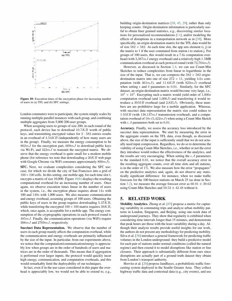
For the sake of our evaluation, we run the experiments on a mid-range (rather than a high-end) Android device, as we do not want tolimit deployment only to (possibly higher-income) users that havenewer phones. We use a Samsung Galaxy A3 device, equipped witha 1.2 GHz quad-core Snapdragon 410 processor and 1.5GB RAM,running Lollipop v5.0.2. For our energy consumption analysis, weutilize PowerTutor [1], an Android app for power monitoring. Notethat, although a Javascript implementation of the cryptographic op-erations might not be optimal in terms of efficiency (e.g., comparedto Java), it offers portability among different mobile OSes. Any-way, we have actually benchmarked a Java implementation of thesame operations and obtained similar results.TFL. We start our experiments with the TFL use-case. Recall thatthe TFL data involves 582 ROIs (stations), so each user device,for each time slot t, encrypts a matrix of size 2 · 582, with thefirst row indicating entering the station and the second exiting it.We here remind that the complexity of the aggregation protocoldepends on how many users are assigned to the same group, sincethe blinding factors are derived from public keys of other users inthe group. In Figure 10(a), we plot the execution time, measured onour Android device, of the encryption phase vis-a-vis the numberof users in the group. As expected, running times grow linearly inthe size of the group. For instance, the encryption performed byeach mobile device takes 4.2s with 100 mobile users and 42s with1,000. Therefore, one should probably keep groups at around 200users, which offers a reasonable trade-off between granularity (interms of privacy) and efficiency. Obviously, even if, say, 1 million2Note that the app is easily tunable so that, instead of binary values, thematrix encodes, e.g., duration of user’s presence in each ROI, whether theuser has entered or exited a cell, etc.3https://cordova.apache.org/4https://github.com/indutny/elliptic
(a) TFL
(b) SFC
Figure 10: Execution times of the encryption phase for increasing numberof users in (a) TFL and (b) SFC settings.
London commuters were to participate, the system simply scales byrunning multiple parallel instances with each group, and combiningmultiple aggregates from 5,000 200-user groups.
When assigning users to groups of size 200, in each round of theprotocol, each device has to download 10.7KB worth of publickeys, and transmitting encrypted values for 2 · 582 entries resultsin an overhead of 4.54KB (independently of how many users arein the group). Finally, we measure the energy consumption to be862mJ for the encryption part, 609mJ to download public keysvia Wi-Fi, and 322mJ to transmit the encrypted matrix. We ob-serve that the energy overhead is quite small for a modern mobilephone (for reference we note that downloading a 20KB web pagewith Google Chrome via WiFi consumes approximately 800mJ).
SFC. Next, we evaluate complexities considering the SFC use-case, for which we divide the city of San Francisco into a grid of100×100 cells. In this setting, our mobile app, for each time slot t,encrypts a matrix of size 10,000. Figure 10(b) displays the resultingcomputational overhead for an increasing number of users. Onceagain, we observe execution times linear in the number of usersin the system, i.e., the encryption phase requires about 14s with100 and 149s with 1,000 users. We also measure communicationand energy overhead, assuming groups of 100 users. Obtaining thepublic keys of users in the group requires downloading 5.37KB,while transferring the encrypted 100×100 matrix requires 39KB,which, once again, is acceptable for a mobile app. The energy con-sumption of the cryptographic operations in each protocol round is485mJ . Finally, the communication operations (via WiFi) require306mJ and 2769mJ , respectively.
Succinct Data Representation. We observe that the number ofusers in each group mainly affects the computation overhead, whilethe communication and energy overheads are primarily influencedby the size of the input. In particular, from our experiments above,we notice that the computation/communication/energy is apprecia-bly low when groups are in the order of hundreds of users and ma-trices are in the order of thousands. This means that if aggregationis performed over larger inputs, the protocol would quickly incurhigh energy, communication, and computation overheads, and thiswould remarkably limit the deployability of our techniques.
In fact, even if in the use-cases considered in this paper the over-head is appreciably low, we would not be able to extend to, e.g.,
building origin-destination matrices [38, 45, 29], rather than onlykeeping counts. Origin-destination information is particularly use-ful to obtain finer grained statistics, e.g., discovering similar loca-tions for personalized recommendations [11], and/or modeling theeffects of disruptions in a transportation network as in [38]. Morespecifically, an origin-destination matrix for the TFL data would beof size 582 × 582. At each time slot, the app sets element (i, j) inthe matrix to 1 if the user commuted from station i to station j. Forgroups of 100 users, this would result in a 7.6s computation over-head (with 3,387mJ energy overhead) and a relatively high 1.5MBcommunication overhead at each protocol round (with 72,704mJ).
However, as discussed in Section 2.4, we can use Count-MinSketches to reduce complexities from linear to logarithmic in thesize of the input. That is, we can compress the 582 × 582 origin-destination matrix into one of size 272 × 11, yielding 4.6s com-putation (with 461mJ), and 11.6KB (with 823mJ) overheadwhen setting ε and δ parameters to 0.01. Similarly, for the SFCdataset, an origin-destination matrix would become very large, i.e.,104 × 104. Encrypting such a matrix would yield order of 1,000scomputation overhead (and 1,000J) and transferring it would in-troduce a 39MB overhead (and 2,835J). Obviously, these num-bers are are prohibitive large for a mobile application. Whereas,with succinct data representation the matrix size could reduce to1.9MB (with 138,137mJ transmission overhead), and a compu-tation overhead of 18s (5,422mJ) when using a Count-Min Sketchwith ε, δ parameters both set to 0.01.
Accuracy. Finally, we assess the accuracy loss introduced by thesuccinct data representation. We start by measuring the error inthe aggregate counts on the TFL data, even though, as discussedabove, the size of the input is sufficiently small that we do not actu-ally need input compression. Regardless, we do so to determine theviability of using Count-Min Sketches, i.e., whether or not the errorthey introduce would reduce the effectiveness of the analytics, andthe results are very encouraging. When setting the ε, δ parametersto the standard 0.01, we notice that the overall accuracy error inthe resulting aggregate counts, over all time slots and all stations,is in the order of 1%. We also measure how the error “propagates”on the predictive analytics and, again, do not observe any statis-tically significant difference: for instance, when we make trafficforecasts for the 100 busiest stations on March 25 (as done in Sec-tion 3.2), we measure the average forecast error as 60.81 ± 39.62using Count-Min Sketches and 59.53± 42.48 without it.
5. RELATED WORKMobility Analytics. Zhong et al. [45] propose a metric for captur-ing variability in commuting trips and analyze urban mobility pat-terns in London, Singapore, and Beijing, using one-week data ofunderground journeys. They show that regularity is exhibited whenconsidering time intervals longer than 15 minutes, and demonstratethat peak hours are those with the least variability during a day. Al-though their analysis results provide useful insights for our work,the authors do not present any methodology for predicting mobility.Silva et al. [38] introduce a general framework for predicting trafficvolumes in the London underground: they build a predictive modelfor each pair of stations under normal conditions (called the naturalregime) and then extend it to model disruptions like station or lineclosures. Their approach is substantially different from ours sincedisruptions are actually part of a ground truth dataset they obtainfrom London’s transport authority.
Horvitz et al. [20] propose JamBayes, a probabilistic traffic fore-casting system deployed in the Seattle Greater Area. They collecthighway traffic data and contextual data (e.g., city events), and use
Bayesian structure search to model bottlenecks. Additionally, usingdata of historic traffic surprises, in combination with recent databefore an event, their system learns Bayesian networks that inferthe likelihood of a future surprise event. Garzó et al. [17] use dis-tributed streaming algorithms to process large scale mobility dataand make user mobility predictions on large metropolitan areas.They evaluate their location prediction methods on a 2-week mo-bility dataset obtained from the Orange D4D challenge [7]. Yavaset al. [42] use data mining to predict user movements in a mobilecomputing system and evaluate their algorithms on a simulated mo-bidity dataset. Overall, prior work on mobility analytics differ fromours as they do not consider collecting data directly from users (northe privacy implications thereof).Detecting Traffic Anomalies. In [30], Pan et al. combine mobil-ity data along with social media to uncover the road network sub-graph associated with an anomaly, based on the routing behavior ofdrivers. Their system is evaluated on the Beijing taxi traces dataset.Similarly, Thom et al. [41] present a system geared to detect spatio-temporal anomalies by performing clustering on geolocated Twit-ter messages and visualize them using tag clouds. They experimentwith three case-studies: an earthquake on the US East Coast, Lon-don riots, and hurricane Irene. Barria et al. [5] present an anomalydetection algorithm for road traffic using microscopic traffic vari-ables like relative speed of vehicles, inter-vehicle time gap, andlane changing, and evaluate their approach using real-world videoimages from a highway segment in Bangkok. Zheng et al. [44] in-vestigate whether collective detection of anomalies from multiplespatio-temporal datasets is possible. They propose a probabilisticanomaly detection method based on a spatio-temporal likelihoodratio test and evaluate it on five datasets from New York City. Sunet al. [40] build Markov models on user mobility patterns in a cellu-lar network, aiming to detect intrusions in the network. Note that,although we also focus on identifying event mobility anomalies,unlike these works, we do so using aggregate crowd-sourced loca-tion data – specifically, collected directly from users in a privacy-preserving way.Private Statistics. Prior work has also proposed a number of toolsto privately gather location statistics, however, they do not demon-strate how these statistics can actually be used for performing mo-bility analytics, which is one of our main goals. Ho et al. [19] ap-ply differential privacy to discover interesting geographic locationson aggregate location data, whereas [27] relies on synthetic datageneration for publishing statistical information about commutingpatterns. Brown et al. [9] propose Haze, a system for privacy-preserving real time traffic statistics based on jury voting proto-cols and differential privacy. Their system hides individual datawhile allowing aggregate information to be collected at the serviceprovider. Similarly, Popa et al. [34] present PrivStats, a systemfor computing aggregate statistics over location data achieving pri-vacy and accountability. Kopp et al. [23] also propose a frame-work enabling the collection of quantitative visits to sets of loca-tions following a distributed approach. Shi et al. [37] show how anuntrusted data aggregator can learn statistics over multiple partici-pants’ private data using cryptographic techniques along with a datarandomization procedure for achieving distributed differential pri-vacy, while Melis et al. [28] demonstrate how to combine privacy-preserving aggregation with succinct data structures (Count-MinSketches [13]) to efficiently compute statistics whilst provably pro-tecting privacy of single data points. They also consider aggregat-ing location information as a possible application of their protocolsbut do not perform any analytics. PASTE [35] introduces a solutionin a similar setting whereby distributed differential privacy is usedon time series data using a Fourier perturbation algorithm.
Finally, Fan et al. [15] propose FAST, an adaptive system for re-leasing real-time aggregate statistics with differential privacy. Theirapproach is based on a trusted central authority that adaptively sam-ples the time series according to detected data dynamics to min-imize the overall privacy budget. They employ Kalman filteringto predict data at non-sampling points and estimate the true val-ues from perturbed ones at sampling in order to improve the accu-racy of data release. In follow-up work [16], they present a genericdifferentially-private framework for anomaly detection on aggre-gate statistics, focusing on detecting epidemic outbreak: real-timeaggregate data is perturbed using FAST [15] and released to an un-trusted entity that performs the anomaly detection task. Whereas,we do not use differential privacy to protect users’ privacy, as thiswould require the presence of a trusted aggregator and introduce atrade-off between privacy and utility that is challenging to tune.
6. CONCLUSIONThis work investigated the feasibility of performing crowd-
sourced mobility analytics over aggregate location data, in a set-ting where users periodically report locations to a server, in sucha way that the server can only recover aggregates, thanks to theuse of a privacy-preserving aggregation protocol. We experimentedwith real-world mobility datasets obtained from the Transport ForLondon authority as well as the San Francisco Cabs network, anddemonstrated that aggregate location data can be useful for pre-dictive analytic tasks like forecasting traffic volumes in regions ofinterest (ROIs) and detecting anomalies in them, using a method-ology based on time series modeling with seasonality. In the pres-ence of traffic anomalies, we also showed how to enhance theirtraffic volume predictions using additional information from cor-related ROIs. Finally, we proposed a privacy-respecting systemfor data collection, and prototyped a mobile application – MobilityData Donors (MDD) – which we empirically evaluated in terms ofcomputation, communication, and energy overhead.
As part of future work, we plan to evaluate our methodology ondifferent location datasets as well as perform a thorough (differen-tial) privacy analysis of releasing datasets composed of aggregatelocations, focusing on group sizes and semantic characteristics ofROIs such as size and density, and their evolution over time.Acknowledgments. The authors wish to thank Luca Melis, GeorgeDanezis, Mirco Musolesi, and Licia Capra for their useful feedbackand/or help with the experiments and the datasets. This research issupported by a Xerox University Affairs Committee grant on “Se-cure Collaborative Analytics.”
7. REFERENCES[1] Power Tutor – A power monitor for Android-Based Mobile
Platforms. http://ziyang.eecs.umich.edu/projects/powertutor/.[2] TFL Budget Report 2015-2016. http://content.tfl.gov.uk/
board-20150326-part-1-item08-tfl-budget-2015-16.pdf.[3] Transport For London - Travel Alerts.
https://twitter.com/tfltravelalerts?lang=el.[4] Waze. https://www.waze.com.[5] J. A. Barria and S. Thajchayapong. Detection and
classification of traffic anomalies using microscopic trafficvariables. IEEE Transactions on Intelligent TransportationSystems, 2011.
[6] D. J. Bernstein, N. Duif, T. Lange, P. Schwabe, and B.-Y.Yang. High-speed high-security signatures. Journal ofCryptographic Engineering, 2012.
[7] V. D. Blondel, M. Esch, C. Chan, F. Clérot, P. Deville,E. Huens, F. Morlot, Z. Smoreda, and C. Ziemlicki. Data for
Development: The D4D Challenge on Mobile Phone Data.arXiv 1210.0137, 2012.
[8] G. E. Box, G. M. Jenkins, G. C. Reinsel, and G. M. Ljung.Time Series Analysis: Forecasting and Control. John Wiley& Sons, 2015.
[9] J. W. Brown, O. Ohrimenko, and R. Tamassia. Haze:Privacy-preserving real-time traffic statistics. In ACMSIGSPATIAL, 2013.
[10] V. Chandola, A. Banerjee, and V. Kumar. Anomalydetection: A survey. ACM computing surveys (CSUR), 2009.
[11] M. Clements, P. Serdyukov, A. P. de Vries, and M. J.Reinders. Personalised travel recommendation based onlocation co-occurrence. arXiv 1106.5213, 2011.
[12] G. W. Corder and D. I. Foreman. Nonparametric Statistics:A Step-by-Step Approach. John Wiley & Sons, 2014.
[13] G. Cormode and S. Muthukrishnan. An Improved DataStream Summary: The Count-Min Sketch and ItsApplications. Journal of Algorithms, 2005.
[14] D. A. Dickey and W. A. Fuller. Distribution of the estimatorsfor autoregressive time series with a unit root. Journal of theAmerican Statistical Association, 1979.
[15] L. Fan and L. Xiong. Real-time aggregate monitoring withdifferential privacy. In ACM CIKM, 2012.
[16] L. Fan and L. Xiong. Differentially private anomalydetection with a case study on epidemic outbreak detection.In IEEE ICDMW, 2013.
[17] A. Garzó, A. A. Benczúr, C. I. Sidló, D. Tahara, and E. F.Wyatt. Real-time streaming mobility analytics. In IEEEInternational Conference on Big Data, 2013.
[18] P. Golle and K. Partridge. On the anonymity of home/worklocation pairs. In Pervasive Computing. Springer, 2009.
[19] S.-S. Ho and S. Ruan. Differential privacy for locationpattern mining. In SIGSPATIAL Workshop on Security andPrivacy in GIS and LBS, 2011.
[20] E. J. Horvitz, J. Apacible, R. Sarin, and L. Liao. Prediction,expectation, and surprise: Methods, designs, and study of adeployed traffic forecasting service. arXiv 1207.1352, 2012.
[21] S. Hylleberg. Seasonality in regression. Academic Press,2014.
[22] M. Jawurek and F. Kerschbaum. Fault-tolerantprivacy-preserving statistics. In PETS, 2012.
[23] C. Kopp, M. Mock, and M. May. Privacy-preservingdistributed monitoring of visit quantities. In ACMSIGSPATIAL, 2012.
[24] J. Krumm. Inference attacks on location tracks. In Pervasive,2007.
[25] K. Kursawe, G. Danezis, and M. Kohlweiss. Privacy-friendlyaggregation for the smart-grid. In PETS, 2011.
[26] W. H. Lam, K. Chan, M. L. Tam, and J. W. Shi. Short-termtravel time forecasts for transport information system in hongkong. Journal of Advanced Transportation, 2005.
[27] A. Machanavajjhala, D. Kifer, J. Abowd, J. Gehrke, andL. Vilhuber. Privacy: Theory meets practice on the map. InIEEE International Conference on Data Engineering, 2008.
[28] L. Melis, G. Danezis, and E. De Cristofaro. Efficient PrivateStatistics with Succinct Sketches. In NDSS, 2016.
[29] M. A. Munizaga and C. Palma. Estimation of a disaggregatemultimodal public transport origin–destination matrix frompassive smartcard data from santiago, chile. TransportationResearch Part C: Emerging Technologies, 2012.
[30] B. Pan, Y. Zheng, D. Wilkie, and C. Shahabi. Crowd sensing
of traffic anomalies based on human mobility and socialmedia. In ACM SIGSPATIAL, 2013.
[31] V. Pandurangan. On Taxis and Rainbows.https://tech.vijayp.ca/of-taxis-and-rainbows-f6bc289679a1.
[32] V. Pejovic and M. Musolesi. Anticipatory mobile computing:A survey of the state of the art and research challenges. ACMComputing Surveys, 2015.
[33] M. Piorkowski, N. Sarafijanovic-Djukic, andM. Grossglauser. CRAWDAD Dataset.http://crawdad.org/epfl/mobility/20090224, 2009.
[34] R. A. Popa, A. J. Blumberg, H. Balakrishnan, and F. H. Li.Privacy and accountability for location-based aggregatestatistics. In ACM CCS, 2011.
[35] V. Rastogi and S. Nath. Differentially private aggregation ofdistributed time-series with transformation and encryption.In ACM SIGMOD, 2010.
[36] G. Sagl, M. Loidl, and E. Beinat. A visual analytics approachfor extracting spatio-temporal urban mobility informationfrom mobile network traffic. ISPRS International Journal ofGeo-Information, 2012.
[37] E. Shi, T. H. Chan, E. Rieffel, R. Chow, and D. Song.Privacy-preserving aggregation of time-series data. In NDSS,2011.
[38] R. Silva, S. M. Kang, and E. M. Airoldi. Predicting trafficvolumes and estimating the effects of shocks in massivetransportation systems. National Academy of Sciences, 2015.
[39] A. Stathopoulos and M. G. Karlaftis. A multivariate statespace approach for urban traffic flow modeling andprediction. Transportation Research Part C: EmergingTechnologies, 2003.
[40] B. Sun, F. Yu, K. Wu, and V. Leung. Mobility-based anomalydetection in cellular mobile networks. In ACM Workshop onWireless Security, 2004.
[41] D. Thom, H. Bosch, S. Koch, M. Wörner, and T. Ertl.Spatiotemporal anomaly detection through visual analysis ofgeolocated twitter messages. In IEEE Pacific VisualizationSymposium, 2012.
[42] G. Yavas, D. Katsaros, Ö. Ulusoy, and Y. Manolopoulos. Adata mining approach for location prediction in mobileenvironments. Data & Knowledge Engineering, 2005.
[43] H. Zang and J. Bolot. Anonymization of location data doesnot work: A large-scale measurement study. In MobiCom,2011.
[44] Y. Zheng, H. Zhang, and Y. Yu. Detecting collectiveanomalies from multiple spatio-temporal datasets acrossdifferent domains. ACM SIGSPATIAL, 2015.
[45] C. Zhong, M. Batty, E. Manley, J. Wang, Z. Wang, F. Chen,and G. Schmitt. Variability in regularity: Mining temporalmobility patterns in london, singapore and beijing usingsmart-card data. PloS One, 2016.