Priors for the Long Run - Federal Reserve Bank of New York · PDF filePriors for the Long Run Domenico ... conomic principles to explicitly model the behavior and interaction of various

This paper presents preliminary findings and is being distributed to economists and other interested readers solely to stimulate discussion and elicit comments.

The views expressed in this paper are those of the authors and do not necessarily reflect the position of the Federal Reserve Bank of New York or the Federal Reserve System. Any errors or omissions are the responsibility of the authors.

Federal Reserve Bank of New York

Staff Reports

Priors for the Long Run

Domenico Giannone

Michele Lenza

Giorgio E. Primiceri

Staff Report No. 832

November 2017

Priors for the Long Run Domenico Giannone, Michele Lenza, and Giorgio E. Primiceri Federal Reserve Bank of New York Staff Reports, no. 832 November 2017 JEL classification: C11, C32, C33, E37

Abstract

We propose a class of prior distributions that discipline the long-run predictions of vector autoregressions (VARs). These priors can be naturally elicited using economic theory, which provides guidance on the joint dynamics of macroeconomic time series in the long run. Our priors for the long run are conjugate, and can thus be easily implemented using dummy observations and combined with other popular priors. In VARs with standard macroeconomic variables, a prior based on the long-run predictions of a wide class of theoretical models yields substantial improvements in the forecasting performance. Key words: Bayesian vector autoregression, forecasting, overfitting, initial conditions, hierarchical model _________________ Giannone: Federal Reserve Bank of New York (email: [email protected]). Lenza: European Central Bank and ECARES (email: [email protected]). Primiceri: Northwestern University, CEPR, and NBER (email: [email protected]). The authors thank Gianni Amisano, Francesco Bianchi, Todd Clark, Gary Koop, Dimitris Korobilis, Ulrich Müller, Christopher Sims, James Stock, Harald Uhlig, Herman K. van Dijk, Mark Watson, and Tao Zha, as well as seminar and conference participants for comments and suggestions. They also thank Patrick Adams and Brandyn Bok for research assistance. The views expressed in this paper are those of the authors and do not necessarily reflect the position of the European Central Bank, the Eurosystem, the Federal Reserve Bank of New York, or the Federal Reserve System.

1. Introduction

Vector Autoregressions (VARs) are flexible statistical models, routinely used for the

description and forecasting of macroeconomic time series, and the analysis of their sources

of fluctuations. The dynamics of these time series are modeled as a function of their

past values and a vector of forecast errors, without imposing any restrictions based on

economic theory. Typically, VARs include many free parameters, to accommodate general

forms of autocorrelations and cross-correlations among variables. With flat priors, however,

such flexibility is likely to lead to in-sample overfitting and poor out-of-sample forecasting

accuracy. For this reason, Bayesian inference with informative priors has a long tradition for

VARs. This paper contributes to this literature by proposing a class of prior distributions

that discipline the long-run behavior of economic variables implied by estimated VARs.

These priors are motivated by a specific form of overfitting of flat-prior VARs, which

is their tendency to attribute an implausibly large share of the variation in observed time

series to a deterministic—and thus entirely predictable—component (Sims, 1996, 2000). In

Date: First version: December 2014. This version: October 2017.

1

PRIORS FOR THE LONG RUN 2

these models, inference is conducted by taking the initial observations of the variables as

non-random. Therefore, the likelihood does not penalize parameter values implying that the

variables’ steady state (for stationary series, their trend for nonstationary ones) is distant

from their initial observations. Complex transient dynamics from these initial conditions to

the steady state are thus implicitly regarded as reasonable. As a consequence, they end up

explaining an implausibly large share of the low frequency variation of the data, yielding

inaccurate out-of-sample forecasts.

One way to address this problem would be to modify inference to explicitly incorporate

the density of the initial observations. This strategy, however, may not be the right solution,

since most macroeconomic time series are (nearly) nonstationary, and it is not obvious how

to specify the distribution of their initial observations (examples of studies trying to address

this issue include Phillips, 1991a,b, Kleibergen and van Dijk, 1994, Uhlig, 1994a,b and, more

recently, Mueller and Elliott, 2003, and Jarocinski and Marcet, 2015, 2011). Following Sims

and Zha (1998) and Sims (2000), an alternative route is to formulate a prior that expresses

disbelief in an excessive explanatory power of the deterministic component of the model,

by specifying that initial conditions should not be important predictors of the subsequent

evolution of the series. However, there are a variety of specific ways to implement this

general idea, especially in a multivariate setting.

Our main insight is that economic theory should play a central role for the elicitation of

these priors, which we base on the robust predictions of another popular class of macroeco-

nomic models, often referred to as dynamic stochastic general equilibrium (DSGE) models.

Relative to VARs, DSGE models are positioned at the opposite side of the spectrum in

terms of their economic-theory content. The DSGE methodology, in fact, uses microe-

conomic principles to explicitly model the behavior and interaction of various economic

agents, such as households, production firms, financial institutions, the government, etc.

This theoretical sophistication comes at the cost of tight cross-equation restrictions on the

joint dynamics of macroeconomic variables, which result in a loss of flexibility and higher

risk of misspecification relative to VARs. On the other hand, the reliance on common eco-

nomic principles implies that different DSGE models usually have some robust predictions,

especially about the long-run behavior of certain variables.1

1In turn, some of the basic economic principles at the root of DSGE models are designed to make theirimplications consistent with the so-called Kaldor’s facts about economic growth, mostly based on pre-WWII


For example, most DSGE models predict that long-run growth in an economy’s aggregate

production, consumption and investment should be driven by a common stochastic trend,

related to technological progress. In fact, advances in the production technology transform-

ing labor and capital inputs into final output should lead to a permanent increase in sales

and people’s average income, as well as their expenditure for the purchase of consumption

and investment goods. In addition, if the production technology has constant returns to

scale—i.e. is homogeneous of order one, a standard assumption in DSGE models—the long-

run impact of technological progress on these variables should be similar, so that the ratio

between consumption or investment expenditure and output should not exhibit a trending

pattern. This is the type of long-run theoretical predictions that we use to elicit our priors

for VARs.

Consistent with these predictions, in a VAR with output, consumption and investment,

we might want to formulate a prior according to which the initial level of the stochastic trend

common to these three variables should explain very little of the subsequent dynamics of the

system. On the other hand, the initial conditions of the consumption- and investment-to-

output ratios should have a higher predictive power. In fact, if these ratios are really mean

reverting, they should converge back to their equilibrium values, and it is thus reasonable

that their initial conditions could shape the low frequency dynamics in the early part of

the sample.

Our prior for the long run (PLR) is a formalization of this general concept. Its key

ingredient is the choice of two orthogonal vector spaces, corresponding to the set of linear

combinations of the model variables that are a-priori likely to be stationary and nonsta-

tionary. It is exactly for the identification of these two orthogonal spaces that economic

theory plays a crucial role. The PLR essentially consists of shrinking the VAR coefficients

towards values that imply little predictive power of the initial conditions of all these linear

combinations of the variables, but particularly so for those that are likely to be nonstation-

ary.

This idea of imposing priors informed by the long-run predictions of economic theory is

reminiscent of the original insight of cointegration and error-correction models (e.g. Engle

and Granger, 1987, Watson, 1994). However, our methodology differs from the classic

data. Kaldor (1961) suggested these stylized facts as starting points for the construction of theoreticalmodels.


literature on cointegration along two main dimensions. First of all, our fully probabilistic

approach does not require to take a definite stance on the cointegration relations and

the common trends—the set of stationary and nonstationary linear combinations of the

variables—, but only on their plausible existence. Therefore, it avoids the pre-testing and

hard restrictions that typically plague error-correction models. More important, the focus

of the cointegration literature is on identifying nonstationary linear combinations of the

model variables, and dogmatically imposing that they cannot affect the short-run dynamics

of the model, while remaining completely agnostic about the impact of the stationary

combinations. On the contrary, we argue that shrinking the effect of these stationary

combinations—albeit more gently—towards zero is at least as important as disciplining the

impact of the common trends.

While we postpone the detailed description of our proposal to the main body of the

paper, here we stress that our PLR is conjugate, and can thus be easily implemented

using dummy observations and combined with existing popular priors for VARs. Moreover,

conjugacy allows the closed-form computation of the marginal likelihood, which can be

used to select the tightness of our PLR following an empirical Bayes approach, or conduct

fully Bayesian inference on it based on a hierarchical interpretation of the model (Giannone

et al., 2015).

We apply these ideas to the estimation of two popular VARs with standard macroeco-

nomic variables. The first is a small-scale model with real GDP, consumption and invest-

ment, as in our previous example. The second, larger-scale VAR also includes two labor

market variables—real labor income and hours worked—and two nominal variables, namely

price inflation and the short-term interest rate. In both cases, we set up our PLR based

on the robust lessons of a wide class of DSGE models. As discussed above, they typically

predict the existence of a common stochastic trend driving the real variables, and possibly

another trend for the nominal variables, while the ratios are likely to be stationary. We show

that a PLR set up in accordance with these theoretical predictions is successful in reducing

the explanatory power of the deterministic component implied by flat-prior VARs. To the

extent that such explanatory power is spurious, this is a desirable feature of the model. In

fact, a VAR with the PLR improves over more traditional Bayesian Vector Autoregressions

(BVARs) in terms of out-of-sample forecasting performance, especially at long horizons.


The accuracy of long-term forecasts is of direct importance in many VAR applications,

including the estimation of impulse response functions, obtained as the difference between

conditional and unconditional forecasts. The scope of our results, however, extends beyond

the usefulness of long-horizon predictions per se. In fact, the analysis of long-run forecasts

appears to be a particularly useful device to detect spurious deterministic overfitting, a

type of model misspecification that can affect all other aspects and uses of VARs.

The rest of the paper is organized as follows. Section 2 explains in what sense flat-prior

VARs attribute too much explanatory power to initial conditions and deterministic trends.

Section 3 illustrates our approach to solve this problem, i.e. our PLR. Section 4 puts our

contribution in the context of a vast related literature, which is easier to do after having

discussed the details of our procedure. Section 5 describes the results of our empirical

application. Section 6 discusses some limitations of our approach and possible extensions

to address them. Section 7 concludes.

2. Initial Conditions and Deterministic Trends

In this section, we show that flat-prior VARs tend to attribute an implausibly large

share of the variation in observed time series to a deterministic—and thus entirely pre-

dictable—component. This problem motivates the specific prior distribution proposed in

this paper. Most of the discussion in this section is based on the work of Sims (1996, 2000),

although our recipe to address this pathology differs from his, as we will see in section 3.

To illustrate the problem, let us begin by considering the simple example of an AR(1)

model,

(2.1) yt = c+ ⇢yt�1 + "t.

Equation (2.1) can be iterated backward to obtain

(2.2) yt = ⇢t�1y1 +t�2X

j=0

⇢jc

| {z }DCt

+t�2X

j=0

⇢j"t�j

| {z }SCt

,

which shows that the model separates the observed variation of the data into two parts.

The first component of (2.2)—denoted by DCt—represents the counterfactual evolution

of yt in absence of shocks, starting from the initial observation y1. Given that AR and


VAR models are typically estimated treating the initial observation as given and non-

random, DCt corresponds to the deterministic component of yt. The second component of

(2.2)—denoted by SCt—depends instead on the realization of all the shocks between time

2 and t, and thus corresponds to the unpredictable or stochastic component of yt.

To analyze the properties of the deterministic component of yt, it is useful to rewrite

DCt as

DCt =

8><

>:

y1 + (t� 1) c if ⇢ = 1

c1�⇢ + ⇢t�1

⇣y1 � c

1�⇢

⌘if ⇢ 6= 1

.

If ⇢ = 1, the deterministic component is a simple linear trend. If instead ⇢ 6= 1, DCt is an

exponential, and has a potentially more complex shape as a function of time. The problem is

that, when conducting inference, these potentially complex deterministic dynamics arising

from estimates of ⇢ 6= 1 can be exploited to fit the low frequency variation of yt, even when

such variation is mostly stochastic. This peculiar “overfitting” behavior of the deterministic

component is clearly undesirable. According to Sims (2000), it is due to two main reasons.

First, the treatment of initial observations as non-stochastic removes any penalization in

the likelihood for parameter estimates that imply a large distance between y1 and c1�⇢ (the

unconditional mean of the process in the stationary case) and, as such, magnifies the effect

of the ⇢t�1 term in DCt. Second, the use of a flat prior on (c, ⇢) implies an informative prior

on⇣

c1�⇢ , ⇢

⌘, with little density in the proximity of ⇢ = 1, and thus on an approximately

linear behavior of DCt.

Sims (2000) illustrates this pathology by simulating artificial data from a random walk

process, and analyzing the deterministic component implied by the flat-prior parameter

estimates of an AR(1) model. By construction, all the variation in the simulated data is

stochastic. Nevertheless, the estimated model has the tendency to attribute a large fraction

of the low frequency behavior of the series to the deterministic component, i.e. to a path

of convergence from unlikely initial observations to the unconditional mean of the process.

In addition, Sims (2000) argues that the fraction of the sample variation due to the de-

terministic component converges to a non-zero distribution, if the data-generating process

is a random walk without drift. We formally prove this theoretical result in appendix A,

and show that it also holds when the true data-generating process is local-to-unity. Put


differently, if the true data-generating process exhibits a high degree of autocorrelation, es-

timated AR models will imply a spurious explanatory power of the deterministic component

even in arbitrarily large samples.

The problem is much worse in VARs with more variables and lags, since these models

imply a potentially much more complex behavior of the deterministic trends. For example,

the deterministic component of an n-variable VAR with p lags is a linear combination of n·p

exponential functions plus a constant term. As a result, it can reproduce rather complicated

low-frequency dynamics of economic time series.

To illustrate the severity of the problem in concrete applications, consider a popular

benchmark VAR that includes seven fundamental macroeconomic variables, i.e. GDP,

consumption, investment, labor income, hours worked (all in log, real and per-capita terms),

price inflation and a short-term nominal interest rate (Smets and Wouters, 2007, Del Negro

et al., 2007).2 Suppose that a researcher is estimating this model using 5 lags and forty years

of quarterly data, from 1955:I to 1994:IV. The dash-dotted lines in figure 2.1 represent the

deterministic components implied by the flat-prior (OLS) estimates for six representative

time series. These deterministic components are obtained as the multivariate generalization

of DCt in 2.2, and thus correspond to the estimated model-implied counterfactual evolution

of these variables in absence of shocks, starting from the initial 5 observations of the sample.

For comparison, the figure also plots the actual realization of these time series over the

sample from 1955:I to 1994:IV used for estimation (solid-thin lines).

First of all, notice that these deterministic trends are more complex at the beginning

of the sample. For instance, the predictable component of the investment-to-GDP ratio

fluctuates substantially between 1955 and 1970, more so than in the rest of the sample. In

addition to exhibiting this marked temporal heterogeneity (Sims, 2000), the deterministic

component also seems to explain a large share of the variation of these time series. Con-

sistent with theory, this feature is most evident for the case of persistent series without (or

with little) drift, such as hours, inflation, the interest rate or the investment-to-GDP ratio.

For instance, the estimated model implies that most of the hump-shaped low-frequency

behavior of the interest rate was due to deterministic factors, and was thus predictable

since as far back as 1955 for a person with the knowledge of the VAR coefficients. And so

was the fact that interest rates would become extremely low around 2010.

2We will describe the variables and data of this application in more detail in section 5.


1960 1970 1980 1990 2000 2010

5.5

6

6.5log-real per-capita GDP

1960 1970 1980 1990 2000 2010

4

4.2

4.4

4.6

4.8

5log-real per-capita investment

1960 1970 1980 1990 2000 2010

-0.65

-0.6

-0.55

-0.5

log hours worked

1960 1970 1980 1990 2000 2010

-1.7

-1.6

-1.5

-1.4

-1.3

log investment-to-GDP ratio

1960 1970 1980 1990 2000 2010

-0.01

0

0.01

0.02

inflation rate

1960 1970 1980 1990 2000 2010

-0.01

0

0.01

0.02

0.03

0.04

interest rate

Data Flat MN PLR

Figure 2.1. Deterministic component for selected variables implied by various 7-variable VARs. Flat: BVAR with a flat prior; MN: BVAR with the Minnesota prior;PLR: BVAR with the prior for the long run.

Most economists would be skeptical of this likely spurious explanatory power of determin-

istic trends, and may want to downplay it when conducting inference. In principle, “one way

to accomplish this is to use priors favoring pure unit-root low frequency behavior” (Sims,

2000, pp. 451), according to which implausibly precise long-term forecasts are unlikely.

However, it is not obvious how to formulate such a prior. For example, the undesirable

properties of the deterministic component persist even when using the popular Minnesota

prior, which is centered on the assumption that all variables in the VAR are random walks

with drift (Litterman, 1979, see also appendix B for a detailed description). When the

tightness of this prior is set to conventional values in the literature (see appendix C), the

implied deterministic components are similar to those of the flat-prior case, as shown by

the dashed lines in figure 2.1. In the next section we detail our specific proposal regarding

how to address this problem.


3. Elicitation of a Prior for the Long Run

Consider the VAR model

(3.1) yt = c+B1yt�1 + ..+Bpyt�p + "t

"t ⇠ i.i.d. N (0,⌃) ,

where yt is an n ⇥ 1 vector of endogenous variables, "t is an n ⇥ 1 vector of exogenous

shocks, and c, B1,..., Bp and ⌃ are matrices of suitable dimensions containing the model’s

unknown parameters. The model can be rewritten in terms of levels and differences

(3.2) �yt = c+⇧yt�1 + �1�yt�1...+ �p�1�yt�p+1 + "t,

where ⇧ = (B1 + . . .+Bp)� In and �j = �(Bj+1 + . . .+Bp), with j = 1, ..., p� 1.

The aim of this paper is to elicit a prior for ⇧. To address the problems described

in the previous section, we consider priors that are centered around zero. As for the prior

covariance matrix on the elements of ⇧, our main insight is that its choice must be guided by

economic theory, and that alternative—automated or “theory-free”—approaches are likely

to lead to a prior specification with undesirable features.

To develop this argument, let H be any invertible n�dimensional matrix, and rewrite

(3.2) as

(3.3) �yt = c+ ⇤yt�1 + �1�yt�1...+ �p�1�yt�p+1 + "t,

where yt�1 = Hyt�1 is an n⇥1 vector containing n linearly independent combinations of the

variables yt�1, and ⇤ = ⇧H�1 is an n⇥n matrix of coefficients capturing the effect of these

linear combinations on �yt. In this transformed model, the problem of setting up a prior

on ⇧ corresponds to choosing a prior for ⇤, conditional on the selection of a specific matrix

H. What is a reasonable prior for ⇤ will then depend on the choice of H. For example,

consider an H matrix whose i�th row contains the coefficients of a linear combination of

y that is a priori likely to be mean reverting. Then, it would surely be unwise to place a

prior on the elements of the i�th column of ⇤ that is excessively tight around zero. In

fact, following the standard logic of cointegration, if the elements of the i�th column of ⇤

were all zero, there would not be any “error-correction” mechanism at play to preserve the

stationarity of this linear combination of y. A similar logic would suggest that, if a row of


H contains the coefficients of an a-priori likely nonstationary linear combination of y, one

can afford more shrinkage on the elements of the corresponding column of ⇤.

This simple argument suggests that it is important to set up different priors on the

loadings associated with linear combinations of y with different degrees of stationarity.

This objective can be achieved by formulating a prior on ⇤, conditional on a choice of H

that combines the data in a way that a-priori likely stationary combinations are separated

from the nonstationary ones.

Interestingly, in many contexts, economic theory can provide useful information for choos-

ing a matrix H with these characteristics. For example, according to the workhorse macroe-

conomic model, output, consumption and investment are likely to share a common stochas-

tic trend, while both the consumption-to-output and the investment-to-output ratios should

be stationary variables. Similarly, standard economic theory would predict that the price

of different goods might be trending, while relative prices should be mean reverting (in

absence of differential growth in the production technology of these goods).3 If these state-

ments were literally true, the corresponding VARs would have an exact error-correction

representation, as in Engle and Granger (1987), with a reduced-rank ⇧ matrix. In practice,

it is difficult to say with absolute confidence whether certain linear combinations of the

data are stationary or integrated. It might therefore be helpful to work with a prior density

that is based on some robust insights of economic theory, while also allowing the posterior

estimates to deviate from them, based on the likelihood information.

We operationalize these ideas by specifying the following prior distribution on the load-

ings ⇤ (as opposed to ⇧), conditional on a specific choice of the matrix H:

(3.4) ⇤·i|Hi·,⌃ ⇠ N⇣0, �i (Hi·)⌃

⌘, i = 1, ..., n,

where ⇤·i denotes the i-th column of ⇤, and �i (Hi·) is a scalar hyperparameter that is

allowed to depend on Hi·, the i-th row of H. For tractability, we also assume that these

priors are scaled by the variance of the error ⌃, are independent across i’s and Gaussian,

which guarantees conjugacy. Notice, however, that the assumption that the priors on the

columns of ⇤ are independent from each other does not rule out (and will in general imply)

3Economic theory usually identifies the set of nonstationary combinations of the model variables, and thespace spanned by the stationary combinations. To form the H matrix, our baseline PLR requires theselection of one specific set of linear combinations belonging to this space. In section 6, we also develop anextension of our methodology that is invariant to rotations within this space.


that the priors on the columns of ⇧ are correlated, with a correlation structure that depends

on the choice of H and �.

The tightness of the prior in (3.4) is controlled by the hyperparameter �i (Hi·). One way

to choose its value is based on subjective considerations. An alternative (empirical Bayes)

strategy is to set �i (Hi·) by maximizing the marginal likelihood, which is the likelihood of

the model only as a function of the hyperparameters, and can be interpreted as a measure

of 1- or multi-step-ahead out-of-sample density-forecast accuracy (Geweke, 2005). Thanks

to the conjugacy of the prior, the marginal likelihood is available in closed form and is

thus very easy to compute. A third option, in between these two extremes, is to adopt a

hierarchical interpretation of the model, and set �i (Hi·) based on its posterior distribution,

which combines the marginal likelihood with a hyperprior (Giannone et al., 2015). This

is the approach that we adopt in our empirical applications. In the next subsection, we

describe a reference parameterization that facilitates the choice of hyperpriors or subjective

values for �i (Hi·).

3.1. Reference value for �i. A crucial element of the density specified in (3.4) is the fact

that �i can be a function of Hi·, which is consistent with the intuition that the tightness

of the prior on the loadings ⇤·i should depend on whether these loadings multiply a likely

stationary or nonstationary linear combination of y from an a-priori perspective. To capture

this important insight, we propose a reference parameterization of �i as follows:

(3.5) �i(Hi.) =�2i

(Hi·y0)2 ,

where �i is a scalar hyperparameter (controlling the standard deviation of the prior on the

elements of ⇤·i), and y0 =1p

Pps=1 ys is a column vector containing the average of the initial

p observations of each variable of the model (these are the observations taken as given in the

computation of the likelihood function). Therefore, the denominator of (3.5) corresponds

to the square of the initial value of the linear combination at hand.

There are a few reasons why this reference formulation is appealing. First of all, sub-

stituting (3.5) into (3.4) makes it clear that the prior variance of ⇤·i has a scaling that

is similar to that of the likelihood, with the variance of the error at the numerator, and

the (sum of) squared regressor(s) at the denominator (recall, for instance, the form of the

variance of the OLS estimator). Second, expression (3.5) captures the insight that tighter


priors are more desirable for the loadings of nonstationary linear combinations of y, which

are likely to have larger initial values (assuming that the data generating process has been

in place for a long enough period of time before the observed sample).4 Third, scaling the

prior variance by 1/ (Hi·y0)2 is more attractive than any alternative scale meant to capture

the same idea, because in this way the prior setup does not rely on any information that

is also used to construct the likelihood function, avoiding any type of “double counting” of

the data.

In the reference parameterization (3.5), the prior tightness is controlled by the hyperpa-

rameter �i, which is just a monotone transformation of �i. Therefore, from a theoretical

point of view, the problem of choosing �i is identical to selecting �i, and can also be based on

subjective considerations, the maximization of the marginal likelihood, or a combination of

the two.5 In practice, however, the choice of a specific subjective value—or a hyperprior—is

easier for �i than for �i, because it has a more direct connection with the problem of the

initial conditions and deterministic trends that we have highlighted in section 2. We clarify

this point in the next subsection, where we explain how to implement this prior using simple

dummy observations, and provide some additional insights into its interpretation.

3.2. Implementation with dummy observations. The prior in (3.4) can be rewritten

in a more compact form as

(3.6) vec (⇤) |H,⌃ ⇠ N⇣0, �H ⌦ ⌃

⌘,

with �H = diag⇣h

�1 (H1·) , ..., �n (Hn·)i⌘

, where vec (·) is the vectorization operator, and

diag (x) denotes a diagonal matrix with the vector x on the main diagonal. Since ⇧ = ⇤H,

the implied prior on the columns of ⇧ is given by

(3.7) vec (⇧) |H,⌃ ⇠ N⇣0, H 0�HH ⌦ ⌃

⌘.

4More specifically, suppose that the true data-generating process of Hi·yt has been in place for a numberof periods T0, where T0 is proportional to the observed sample size T . In the stationary case, (Hi·y0)

2 isbounded in probability. It is instead of order T in the integrated or local-to-unity case, where is equalto 1 or 3/2 depending on the presence of the drift. Notice, however, that this asymptotic logic might befragile in finite samples, if a combination of the y’s is stationary around a very large mean. In such cases,the value of (Hi·y0)

2 would be unduly large, implying an excessively tight prior. This is one of the reasonswhy the flexibility provided by the hyperparameter �i discussed below is important.5For example, given the invariance property of maximum likelihood, an empirical Bayes approach basedon the maximization of the marginal likelihood would lead to identical inference regardless of whether oneuses this specific parameterization or not.


Being conjugate, this prior can be easily implemented using Theil mixed estimation, i.e.

by adding a set of n artificial (or dummy) observations to the original sample. Each of

these n dummy observations consists of a value of the variables on the left- and right-hand

side of (3.1), at an artificial time t⇤i . In particular, the implementation of the prior in (3.7),

with the parameterization of �i in (3.5), requires the following set of artificial observations:

(3.8) yt⇤i = yt⇤i�1 = ... = yt⇤i�p =Hi·y0�i

⇥H�1

⇤·i , i = 1, ..., n,

where the corresponding observation multiplying the constant term is set to zero, and⇥H�1

⇤·i denotes the i-th column of H�1. We prove this result in appendix B, where we

also derive the posterior distribution of the model’s unknown coefficients.

To provide yet another interpretation of our prior, it is useful to substitute the dummy

observations (3.8) into the level-difference representation of the model (3.2), obtaining

(3.9) 0 = ⇧⇥H�1

⇤·i| {z }

⇤·i

(Hi·y0) + �i"t⇤i , i = 1, ..., n.

This expression suggests that the prior is effectively limiting the extent to which the linear

combinations Hi·y help forecasting �y at the beginning of the sample. This feature reduces

the importance of the error-correction mechanisms of the model, which are responsible for

the complex dynamics and excessive explanatory power of the deterministic component

that we have analyzed in section 2. However, given that the value of Hi·y0 is typically lower

(in absolute value) for mean-reverting combinations of y, our prior reduces more gently the

mechanisms that correct the deviations from equilibrium of likely stationary combinations

of the variables, consistent with the idea of cointegration.

The representation of the prior in terms of dummy observations also provides some useful

insights for the elicitation of a hyperprior. The value of �i = 1 corresponds to using a single

artificial observation in which the linear combination of variables on the right- and left-hand

side is equal to its initial condition, with an error variance of this observation similar to

that in the actual sample. Therefore, 1 seems a sensible reference value for �i, and we use

it to center its hyperprior (we also choose 1 as a standard deviation for this hyperprior, see

appendix C for details).


3.3. Simple bivariate example. Before turning to a more comprehensive comparison

with some of the existing literature, it is useful to contrast our PLR to the more standard

sum-of-coefficients prior, first proposed by Doan et al. (1984), and routinely used for the

estimation of BVARs (Sims and Zha, 1998). The sum-of-coefficients prior also disciplines the

sum of coefficients on the lags of each equation of the VAR, but corresponds to mechanically

setting H equal to the identity matrix, even when there might be some linear combinations

of the variables in the system that should be stationary.

For the sake of concreteness, consider the simple example of a bivariate VAR(1) with

log-output (Yt) and log-investment (It). The sum-of-coefficients prior corresponds to

vec (⇧) |⌃ ⇠ N

0

@0,

2

4µ2

Y 20

0

0 µ2

I20

3

5⌦ ⌃

1

A ,

where µ is an hyperparameter controlling its overall tightness. Economic theory, however,

suggests that output and investment are likely to share a common trend (Yt+ It), while the

log-investment-to-output ratio (It�Yt) is expected to be stationary. Based on this insight,

we can form the matrix H, whose rows correspond to the coefficients of these two different

linear combinations of the variables:

(3.10) H =

2

4 1 1

�1 1

3

5 .

One can now ask what is the prior implied by sum-of-coefficients prior on the coefficients

capturing the effect of these two linear combinations on �Yt and �It (i.e. on the error-

correction coefficients, using the cointegration terminology). To answer this question, recall

that ⇤ = ⇧H�1, which implies that vec (⇤) =⇣�

H�1�0 ⌦ In

⌘vec (⇧), and thus

vec (⇤) |H,⌃ ⇠ N

0

@0,1

4

2

4µ2

Y 20+ µ2

I20

µ2

I20� µ2

Y 20

µ2

I20� µ2

Y 20

µ2

Y 20+ µ2

I20

3

5⌦ ⌃

1

A .

Notice that the prior on the loadings of the common trend is as tight as that on the loadings

of the investment ratio, which is in contrast with the predictions of most theoretical models

and with the main insights of cointegration.


On the contrary, our PLR with the choice of H in (3.10) corresponds to the following

prior density on the error-correction coefficients:

vec (⇤) |H,⌃ ⇠ N

0

@0,

2

4�21

(Y0+I0)2 0

0�22

(I0�Y0)2

3

5⌦ ⌃

1

A .

Clearly, even if �1 ⇡ �2, and given that (I0 � Y0)2 is a much smaller number than (Y0 + I0)

2,

this prior performs much less shrinkage on the coefficients that correct the deviations of the

investment ratio from its equilibrium value.

4. Relationship with the Literature

Before turning to the empirical application, it is useful to relate our approach more

precisely to the literature on cointegration (Engle and Granger, 1987) and error-correction

models (for a comprehensive review, see Watson, 1994). For the purpose of making this

comparison as concrete as possible, suppose that the specific model at hand entails a natural

choice of H with the following two blocks of rows:

(4.1) H =

2

664

�0?

(n�r)⇥n

�0r⇥n

3

775 ,

where the columns of �? are (n� r) linear combinations of y that are likely to exhibit a

stochastic trend, while the columns of � are r linear combinations of y that are more likely

to represent stationary deviations from long-run equilibria, i.e. that are likely to correspond

to cointegrating vectors. Using this notation, we can rewrite (3.3) as

(4.2) �yt = c+ ⇤1��0?yt�1

�+ ⇤2

��0yt�1

�+ �1�yt�1...+ �p�1�yt�p+1 + "t,

where ⇤1 are the first n� r columns of ⇤, and ⇤2 are the remaining r columns.

As described in the previous section, our approach consists of placing priors on the

columns of ⇤1 and ⇤2. These priors are centered around zero, and are tighter for the

elements of ⇤1 than for those of ⇤2. The error-correction representation corresponds to

an extreme case of our general model, obtained by enforcing a dogmatic prior belief that

⇤1 = 0. As a result, ⇧ would equal ⇤2�0, and would be rank deficient. If, in addition, the

prior belief that ⇤2 = 0 is also dogmatically imposed, the VAR admits a representation

in first differences. Notice that this is different from imposing a dogmatic version of the


Minnesota prior of Litterman (1979), which would imply not only setting ⇤1 and ⇤2 to 0,

but also �1 = ... = �p�1 = 0, resulting in a specification in which all variables follow a

random walk with drift.

For what concerns the cointegrating vectors �, the literature has proceeded by either

fixing or estimating them. The approach that is closer to ours selects the cointegrating

vectors � a priori, mostly based on economic theory. This strategy is appealing since the

theoretical cointegrating relations are typically quite simple and robust across a wide class of

economic models. Conditional on a specific choice of �, one popular approach is to include

all the theoretical cointegrating vectors in the error-correction representation, and conduct

likelihood-based inference (i.e. OLS), as in King et al. (1991) or Altig et al. (2011). In our

model, this is equivalent to placing a flat prior on ⇤2. An alternative strategy, however, has

been to conduct some pre-testing and to include in the error correction only those deviations

from equilibria for which the adjustment coefficients are statistically significantly different

from zero, as in Horvath and Watson (1995). Conditional on the pre-testing results, this

approach is equivalent to setting a dogmatic prior that certain columns of ⇤2 are equal to

zero, and a flat prior on the remaining elements.

The other strand of the literature is more agnostic about both the cointegrating rank (r)

and the cointegrating vectors (�). In these cases, classical inference is typically conducted

using a multi-step methodology. The first step of these procedures requires testing for the

cointegrating rank. Conditional on the results of these tests, the second step consists of the

estimation of the cointegrating vectors, which are then treated as known in step three for the

estimation of the remaining model parameters (Engle and Granger, 1987). Alternatively,

the second and third steps can be combined to jointly estimate � and the other parameters

with likelihood-based methods, as in Johansen (1995).

The Bayesian approach to cointegration is similar in spirit to the likelihood-based in-

ference (for recent surveys, see Koop et al., 2006, Del Negro and Schorfheide, 2011, and

Karlsson, 2013). This literature has also concentrated on conducting inference on the coin-

tegrating rank and the cointegrating space. For example, the number of cointegrating

relationships is typically selected using the marginal likelihood, or related Bayesian model

comparison methods (Chao and Phillips, 1999, Kleibergen and Paap, 2002, Corander and

Villani, 2004, Villani, 2005). In practical applications, this methodology ends up being

similar to pre-testing because the uncertainty on the cointegrating rank is seldom formally


incorporated into the analysis, despite the fact that the Bayesian approach would allow to

do it (for an exception, see Villani, 2001).

Conditional on the rank, the early Bayesian cointegration literature was concerned with

formulating priors on the cointegrating vectors, and with deriving and simulating their

posterior (Bauwens and Lubrano, 1996, Geweke, 1996). Standard priors, however, have

been shown to be problematic, in light of the pervasive local and global identification issues

of error-correction models (Kleibergen and van Dijk, 1994, Strachan and van Dijk, 2005).

To avoid these problems, a better strategy is to place a prior on the cointegrating space,

which is the only object the data are informative about (Villani, 2000). Such priors are

studied in Strachan and Inder (2004) and Villani (2005), who also develop methods for

inference and posterior simulations. In particular, Villani (2005) proposes a diffuse prior

on the cointegrating space, trying to provide a Bayesian interpretation to some popular

likelihood-based procedures. In general, little attention has been given to the elicitation of

informative priors on the adjustment coefficients, which is instead the main focus of our

paper.

It is well known that maximum-likelihood (or flat-prior) inference in the context of error-

correction models can be tricky (Stock, 2010). This is not only because of the practice to

condition on initial conditions, as we have stressed earlier, but also because inference is

extremely sensitive to the value of non-estimable nuisance parameters characterizing small

deviations from non-stationarity of some variables (Elliott, 1998, Mueller and Watson,

2008). Pretesting is clearly plagued by the same problems. The selection of models based on

pre-testing or Bayesian model comparison can be thought as limiting cases of our approach,

in which the support of the distributions of the hyperparameters controlling the tightness

of the prior on specific adjustment coefficients can only take values equal to zero or infinity.

One advantage of our flexible modeling approach, instead, is that it removes such an extreme

sparsity of the model space, as generally recommended by Gelman et al. (2004) and Sims

(2003).

Finally, our paper is also related to the methodology of Del Negro and Schorfheide (2004)

and Del Negro et al. (2007), who also use a theoretical DSGE model to set up a prior for

the VAR coefficients. Their work, however, differs from ours in two important ways. First

of all, the prior of Del Negro et al. (2007) is centered on the error-correction representation

of the VAR, given that such a prior pushes towards a DSGE model featuring a balanced


growth path. On the contrary, for the reasons highlighted in section 2, our PLR shrinks

the VAR towards the representation in first differences, albeit it does so more gently for

the linear combinations of the variables that are supposed to be stationary according to

theory. In addition, the approach of Del Negro and Schorfheide (2004) requires the complete

specification of a DSGE model, including its short-run dynamics. Instead, we use only the

long-run predictions of a wide class of theoretical models to guide the setup of our PLR.

Among other things, this strategy allows us to work with a conjugate prior and simplify

inference.

5. Empirical Results

In this section we use our prior to conduct inference in VARs with standard macroeco-

nomic variables, whose joint long-run dynamics are sharply pinned down by economic the-

ory. In particular, we perform two related but distinct exercises. We begin by re-estimating

the 7-variable VAR of section 2, to show that our PLR serves the purpose of reducing the

excessive explanatory power of the deterministic components implied by the model with flat

or Minnesota priors. Second, we evaluate the forecasting performance of 3- and 7-variable

VARs, and demonstrate that our prior yields substantial gains over more standard BVARs,

especially when forecasting at long horizons. Before turning to the detailed illustration of

these results, we begin by describing more precisely the 3- and 7-variable VARs and the

priors that we adopt.

The 3-variable VAR includes data on log-real per-capita GDP (Yt), log-real per-capita

consumption (Ct) and log-real per-capita investment (It) for the US economy, and is similar

to the VAR estimated by King et al. (1991) in their influential analysis of the sources of

business cycles. This model is appealing because of its simplicity, popularity, and because

a PLR can be easily elicited based on standard neoclassical growth theory, which is at

the core of DSGE modeling. This theory predicts the existence of a balanced growth path,

along which output, consumption and investment share a common trend, while the so-called

great ratios (the consumption- and investment-to-output ratios) should be stationary.

The 7-variable VAR augments the small-scale model with two labor-market variables—log-

real per-capita labor income (Wt) and log-hours worked per-capita (Ht)—and two nominal

variables—price inflation (⇡t) and the federal funds rate (Rt). These are the same time

series used to estimate the DSGE model of Smets and Wouters (2007), which adds to


the neoclassical core the assumptions that markets are not competitive, and prices and

wages are sticky. This DSGE is representative of modern medium-to-large-scale macroeco-

nomic models, and can thus be used as a guide to set up our prior in this context. This

class of models typically predicts that output, consumption, investment, and labor income

are driven by a common stochastic trend, while the labor share (labor income relative to

output), the consumption- and investment-to-output ratios, and hours worked should be

stationary.

In addition, some New-Keynesian DSGE models (e.g. Ireland, 2007) also include a

stochastic nominal trend, common to the interest and inflation rates. While the existence

of such a stochastic nominal trend is not a robust feature of this class of DSGE models,

most of them do imply that the low-frequency behavior of inflation and interest rates are

tightly related. This is exactly the type of situation in which it might be beneficial to

formulate a prior that is centered on the existence of a common nominal trend, without

imposing it dogmatically.

A compact way of summarizing the variables included in each model and the linear

combinations used to set up our PLR is to illustrate the details of the choice of yt and H

for the larger, 7-variable model:

yt =

2

6666666666666664

1 1 1 1 0 0 0

�1 1 0 0 0 0 0

�1 0 1 0 0 0 0

�1 0 0 1 0 0 0

0 0 0 0 1 0 0

0 0 0 0 0 1 1

0 0 0 0 0 �1 1

3

7777777777777775

| {z }H

0

BBBBBBBBBBBBBBB@

Yt

Ct

It

Wt

Ht

⇡t

Rt

1

CCCCCCCCCCCCCCCA

| {z }yt

! real trend

! log consumption-to-GDP ratio

! log investment-to-GDP ratio

! log labor share

! log hours

! nominal trend

! real interest rate.

The 3-variable VAR only includes the first 3 variables of yt and the 3⇥ 3 upper-left block

of H.6

6In the online appendix, we also present the intermediate case of a 5-variable VAR that includes thefirst 5 variables of yt and the 5 ⇥ 5 upper-left block of H. The online appendix is available here:http://faculty.wcas.northwestern.edu/~gep575/OnlineAppendix_plr4- 1.pdf.


We now turn to the description of the specific exercises that we conduct and the empirical

results.

5.1. Deterministic trends. In section 2, we have argued that a serious pathology of flat-

prior VARs is that they imply rather complex dynamics and excessive explanatory power

of the deterministic component of economic time series (Sims, 1996, 2000). In addition, the

use of the standard Minnesota prior (with conventional hyperparameter values) does very

little, if nothing at all, to solve the problem (figure 2.1). In this subsection, we analyze the

extent to which our PLR eliminates or reduces this pathology.

To this end, we re-estimate the 7-variable VAR with 5 lags of section 2 using our PLR,

and compare the deterministic trends implied by this model to those of section 2, obtained

using a BVAR with flat or Minnesota priors.7 In this experiment, for simplicity, we simply

set the hyperparameters {�i}ni=1 equal to one, which provides a good reference value (it

corresponds to adding one dummy observation, see appendix C).

The results of this experiment are depicted in figure 2.1. In the case of GDP, the dif-

ference between the deterministic component of the BVAR with the PLR and the flat or

Minnesota priors is limited. For the other variables, notice that the shape of the determin-

istic component implied by the PLR is simpler, and explains much less of the low frequency

variation of the time series. For example, in the case of investment, the deterministic trend

implied by the PLR resembles a straight line, implying that the long-run growth rate of

investment in the next decades is expected to be in line with the past. Similarly, in the

case of inflation and the interest rate, the deterministic trend of the BVAR with the PLR

does not have the unpleasant property that somebody with the knowledge of the model

coefficients would have perfectly predicted the hump shape of these two variables already

in 1955.

In sum, our PLR is quite successful in correcting the pathology that we have illustrated

in section 2. In the next section, we will demonstrate that this is not simply a theoretical

curiosity, but that it is extremely important for the forecasting performance of the model.

5.2. Forecasting performance. In this subsection, we compare the forecasting perfor-

mance of our BVAR to a number of benchmark BVARs. More specifically, we consider the

following models:7We conduct this experiment with the 7-variable VAR, as opposed to the 3-variable one, because the problemis more severe in this case.


• MN-BVAR: BVAR with the Minnesota prior, as in the work of Litterman (1979).

This popular prior is centered on the assumption that all variables in the VAR follow

a random walk with drift, which is a parsimonious yet “reasonable approximation

of the behavior of an economic variable” (Litterman, 1979, p. 20). The variance of

this prior is smaller for the coefficients associated with more distant lags, which are

expected to contain less information about the current values of the variables (see

appendix B for a detailed description of this prior).

• SZ-BVAR: BVAR with the Minnesota prior and the sum-of-coefficients (also known

as no-cointegration) prior, as in the work of Doan et al. (1984) and Sims and Zha

(1998). The latter corresponds to our PLR with a mechanical choice of H equal to

the identity matrix, and the same hyperparameter for each dummy observation. It

has the effect of pushing the VAR parameter estimates towards the existence of a

separate stochastic trend for each variable.

• DIFF-VAR: VAR with the variables in first differences, corresponding to an infin-

itely tight PLR or sum-of-coefficients prior.

• PLR-BVAR: BVAR with the Minnesota prior and our PLR.

This comparison of forecasting accuracy is interesting because the first three models are con-

sidered valid benchmarks in the literature. For example, it is well known that MN-BVARs

yield substantial forecasting improvements over classical or flat-prior VARs (Litterman,

1979) and that further improvements can be achieved by adding the sum-of-coefficients

prior of Doan et al. (1984). In fact, Giannone et al. (2015) show that the predictive ability

of the model of Sims and Zha (1998) is comparable to that of factor models. Finally, a VAR

in first differences corresponds to the limit case of an infinitely tight PLR, with as many

stochastic trends as variables. This specification reduces the complexity of the deterministic

components the most, at the cost of also eliminating all error-correction mechanisms in the

model. As we show in the online appendix, the forecasting performance of the DIFF-VAR

is almost identical to that of a naive model in which all the variables follow separate uni-

variate random walks with drifts. A number of papers have demonstrated that this naive

random walk model forecasts quite well, especially after the overall decline in predictability

of macroeconomic time series in 1985 (Atkeson and Ohanian., 2001, Stock and Watson,

2007, D’Agostino et al., 2007, Rossi and Sekhposyan, 2010).


In what follows, our measure of forecasting accuracy is the out-of-sample mean squared

forecast error (MSFE). In particular, for each of the four models, we produce the 1- to

40-quarter-ahead forecasts, starting with the estimation sample that ranges from 1955Q1

to 1974Q4. We then iterate the same procedure updating the estimation sample, one quar-

ter at a time, until the end of the sample in 2013Q1. At each iteration, we choose the

tightness of the priors by maximizing the posterior of the models’ hyperparameters, using

the procedure proposed by Giannone et al. (2015) and summarized in appendix C. Condi-

tional on the selected value of these hyperparameters (reported in the online appendix), we

then produce the out-of-sample forecasts by setting the VAR coefficients to their posterior

mode. All BVARs are estimated using 5 lags, which is slightly above one year to capture

potential residual seasonal factors. For all the forecast horizons, the evaluation sample for

the computation of the MSFEs ranges from 1985Q1 to 2013Q1.

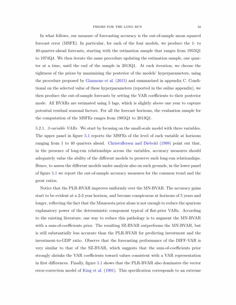
5.2.1. 3-variable VARs. We start by focusing on the small-scale model with three variables.

The upper panel in figure 5.1 reports the MSFEs of the level of each variable at horizons

ranging from 1 to 40 quarters ahead. Christoffersen and Diebold (1998) point out that,

in the presence of long-run relationships across the variables, accuracy measures should

adequately value the ability of the different models to preserve such long-run relationships.

Hence, to assess the different models under analysis also on such grounds, in the lower panel

of figure 5.1 we report the out-of-sample accuracy measures for the common trend and the

great ratios.

Notice that the PLR-BVAR improves uniformly over the MN-BVAR. The accuracy gains

start to be evident at a 2-3 year horizon, and become conspicuous at horizons of 5 years and

longer, reflecting the fact that the Minnesota prior alone is not enough to reduce the spurious

explanatory power of the deterministic component typical of flat-prior VARs. According

to the existing literature, one way to reduce this pathology is to augment the MN-BVAR

with a sum-of-coefficients prior. The resulting SZ-BVAR outperforms the MN-BVAR, but

is still substantially less accurate than the PLR-BVAR for predicting investment and the

investment-to-GDP ratio. Observe that the forecasting performance of the DIFF-VAR is

very similar to that of the SZ-BVAR, which suggests that the sum-of-coefficients prior

strongly shrinks the VAR coefficients toward values consistent with a VAR representation

in first differences. Finally, figure 5.1 shows that the PLR-BVAR also dominates the vector

error-correction model of King et al. (1991). This specification corresponds to an extreme


0 10 20 30 40 0

0.002

0.004

0.006

0.008

0.01

MS

FE

Y

0 10 20 30 40

Quarters ahead

0

0.02

0.04

0.06

0.08

0.1

0.12

0.14

MS

FE

Y + C + I

0 10 20 30 40 0

0.002

0.004

0.006

0.008

0.01

0.012

0.014C

0 10 20 30 40

Quarters ahead

0

0.0005

0.001

0.0015

0.002C - Y

0 10 20 30 40 0

0.01

0.02

0.03

0.04

0.05I

0 10 20 30 40

Quarters ahead

0

0.005

0.01

0.015

0.02

0.025

0.03I - Y

MN SZ DIFF VECM PLR

Figure 5.1. Mean squared forecast errors in models with three variables. MN: BVARwith the Minnesota prior; SZ: BVAR with the Minnesota and sum-of-coefficient priors;DIFF: VAR with variables in first differences; VECM: vector error-correction model thatimposes the existence of a common stochastic trend for Y, C and I, without any additionalprior information; PLR: BVAR with the Minnesota prior and the prior for the long run.

version of the PLR, which dogmatically imposes the existence of a common stochastic

trend for output, consumption and investment, without introducing any additional prior

information.

The key question for us is understanding why the PLR-BVAR outperforms the SZ-BVAR

and the DIFF-VAR. We address this question in figure 5.2, which plots the realized value

of the log consumption- and investment-to-GDP ratios, and the forecasts of these variables

produced 5 years in advance by the PLR-BVAR and the DIFF-VAR (the SZ-BVAR forecasts

are very close to those of the DIFF-VAR, so we do not report them to avoid clogging the

figure). Since the DIFF-VAR imposes the existence of a separate stochastic trend for all

the variables, the difference between log-consumption and log-output, and the difference

between log-investment and log-output are also characterized by stochastic trends. As the


1960 1970 1980 1990 2000 2010

-0.65

-0.6

-0.55

-0.5

C - Y

1960 1970 1980 1990 2000 2010

-1.7

-1.6

-1.5

-1.4

-1.3

I - Y

Actual DIFF PLR

Figure 5.2. Log of the consumption- and investment-to-GDP ratios, and their fore-casts produced 5 years in advance by models with three variables. DIFF: VAR withvariables in first differences; PLR: BVAR with the Minnesota prior and the prior for thelong run.

first panel of figure 5.2 makes clear, an integrated process is a pretty good predictor of

the consumption-to-GDP ratio because this variable displays a (close to) nonstationary

behavior in the data. The no-change long-term forecasts of an integrated process, however,

are poor predictors of the investment-to-GDP ratio at long horizons, because this series

looks mean reverting (second panel of figure 5.2).

The strength of the PLR-BVAR is the ability to push the common trend towards a

unit root approximately as intensely as the SZ-BVAR or the DIFF-VAR, while performing

substantially less shrinkage on the consumption- and investment-to-GDP ratios. Therefore,

this more sophisticated prior does not outweigh the likelihood information about the mean

reversion of the investment ratio, while being consistent with the trending behavior of the

consumption ratio. Finally, notice that the PLR-BVAR would also outperform the purely


theory-based predictions of constant ratios, which is particularly at odds with the observed

pattern of consumption relative to GDP.

Before turning to the VAR with seven variables, we wish to briefly mention another pop-

ular prior—the so called dummy-initial-observation (or single-unit-root, or co-persistence)

prior—used in the existing literature. This elegant prior was designed to remove the bias of

the sum-of-coefficients prior against cointegration, while still addressing the issue regarding

overfitting of the deterministic component (Sims and Zha, 1998). For completeness, we have

experimented with this prior as well, but its marginal impact on the posterior relative to the

Minnesota and sum-of-coefficients priors is negligible, as we show in the online appendix.

Therefore, to save space, we have decided to exclude the dummy-initial-observation prior

from the forecast comparison in the main text.

5.2.2. 7-variable VARs. Turning to the 7-variable case, figures 5.3 and 5.4 plot the MSFEs

for the level of the variables in the VAR and for the linear combinations obtained by

multiplying the matrix H by the vector y (i.e. the common trends, the great ratios and the

real rate). Although there are cases in which all the BVARs perform similarly, the PLR-

BVAR generally improves over the MN-BVAR and SZ-BVAR. The most substantial gains

are evident for the nominal block and consumption (and the linear combinations involving

these variables).

What is interesting about the 7-variable case, however, is that the performance of all the

BVARs specified in levels deteriorates relative to the DIFF-VAR for output, consumption

and wages. Closer inspection reveals that this deterioration is mostly due to the inaccuracy

of the BVARs long-term forecasts produced in the late 1970s. Given the record-high level

of inflation, and the historical negative correlation between current inflation and future

real activity, all the VARs estimated in levels in the late 1970s tend to predict a very

severe and long-lasting drop in output. In reality, instead, the recession of the early 1980s

ended relatively quickly, suggesting the presence of a stronger long-run disconnect between

nominal and real variables than predicted by these models.8

To confirm this view, the dotted lines in figures 5.3 and 5.4 represent the MSFEs produced

by a restricted version of the PLR-BVAR, where we impose that the nominal trend has no

8Observe that we have been able to uncover this interesting misbehavior of VARs estimated with nominalvariables in the 1970s because of our focus on long-term predictions, which are instead typically neglectedby the literature on forecast evaluation.


0 20 40 0

0.002

0.004

0.006

0.008

0.01

MS

FE

Y

0 20 40 0

0.002

0.004

0.006

0.008

0.01

0.012

0.014C

0 20 400

0.01

0.02

0.03

0.04

0.05

0.06

0.07

0.08I

0 20 40 0

0.002

0.004

0.006

0.008

0.01H

0 20 40

Quarters Ahead

0

0.005

0.01

0.015

0.02

MS

FE

W

0 20 40

Quarters Ahead

0

0.00005

0.0001

0.00015

0.0002

0 20 40

Quarters Ahead

0

0.00005

0.0001

0.00015

0.0002

0.00025

0.0003R

MN

SZ

DIFF

PLR

PLR tight

Figure 5.3. Mean squared forecast errors in models with seven variables. MN: BVARwith the Minnesota prior; SZ: BVAR with the Minnesota and sum-of-coefficients priors;DIFF: VAR with variables in first differences; PLR: BVAR with the Minnesota prior andthe prior for the long run; PLR tight: BVAR with the Minnesota prior and the prior forthe long run with maximum tightness on the dynamic effect of the common nominaltrend.

impact on the dynamics of the system. Such a model corresponds to dogmatically setting

to zero the hyperparameter �i controlling the variance of the prior on the column of ⇤ that

captures the effects of the nominal trend. Relative to its unrestricted version, this model

generates better MSFEs for the real variables, getting close to MSFEs of the DIFF-VAR.

However, the figures also show a worsening of the forecasting performance for inflation

and the nominal trend. The reason for this deterioration is that our conjugate prior does

not allow for differential shrinkage on different elements of a column of ⇤.9 Therefore,

eliminating the effect of the nominal trend on real variables, comes at the cost of also

9This is a feature of all conjugate priors with a Kronecker structure, including the Minnesota or sum-of-coefficients priors.


0 20 40 0

0.05

0.1

0.15

0.2

0.25

0.3

MS

FE

Y + C + I + W

0 20 40 0

0.0005

0.001

0.0015

0.002

MS

FE

C - Y

0 20 40 0

0.01

0.02

0.03

0.04

0.05

0.06

MS

FE

I - Y

0 20 40 0

0.002

0.004

0.006

0.008

0.01

MS

FE

H

0 20 40

Quarters Ahead

0

0.0005

0.001

0.0015

0.002

0.0025

0.003

0.0035

MS

FE

W - Y

0 20 40

Quarters Ahead

0

0.0001

0.0002

0.0003

0.0004

0.0005

0.0006

0.0007

MS

FE

R +

0 20 40

Quarters Ahead

0

5e-05

0.0001

0.00015

0.0002

MS

FE

R - MN

SZ

DIFF

PLR

PLR tight

Figure 5.4. Mean squared forecast errors in models with seven variables (linear com-binations). MN: BVAR with the Minnesota prior; SZ: BVAR with the Minnesota andsum-of-coefficients priors; DIFF: VAR with variables in first differences; PLR: BVAR withthe Minnesota prior and the prior for the long run; PLR tight: BVAR with the Minnesotaprior and the prior for the long run with maximum tightness on the dynamic effect of thecommon nominal trend.

impairing any effect of the nominal trend on inflation. Our findings suggest that breaking

this symmetry would be beneficial, although we leave the development of this non-conjugate

type of priors for future research.

6. Invariance to Rotations and Other Challenges

In the previous sections, we have discussed the motivation for our PLR, its most attractive

features and success in applications. We now also want to highlight the potential limitations

of our methodology, and consider extensions that might address some of them.

6.1. Invariance to rotations. In this subsection, we discuss the fact that our prior re-

quires the selection of a specific matrix H. We have argued that the rows of H should


be chosen to represent linear combinations of y that are likely to exhibit a stochastic

trend—denote the coefficients of these combinations by �0?—and stationary deviations from

long-run equilibria—call them �0. Notice that economic theory is useful, but not sufficient

to uniquely pin down a specific H. The reason is that macroeconomic models are typically

informative about �? and the space spanned by � (the cointegrating space), but not about

� itself.

For example, in the case of our three variable VAR, theory suggests that GDP, consump-

tion and investment should share a common trend, and that all the linear combinations

orthogonal to this trend should be stationary. We have implemented our prior selecting the

consumption- and the investment-to-GDP ratios as possibly stationary linear combinations.

While this choice might seem natural, it would have been equally valid to pick for instance

the consumption-to-investment instead of the investment-to-GDP ratio. The baseline PLR

presented in section 3 is not invariant to these rotations of � that, according to theory, are

equally likely to generate stationary linear combinations of the variables.

From a theoretical perspective, this lack of invariance might seem unappealing, but it

should not be considered as a serious concern, in practice. In fact, most of the gains of

our prior derive from separating the common trends from the space of likely stationary

combinations, and hence from shrinking more gently the strength of the error-correction

mechanisms of the latter. Within this “stationary space,” the specific combinations that

one selects to implement the prior matter much less. Nevertheless, to fully tackle the issue

of invariance, in this section we develop a version of our prior that only depends on the

space of stationary combinations implied by economic theory.

Without loss of generality, suppose that the first n�r rows of H represent the coefficients

of the linear combinations of y that are likely to be nonstationary, while the remaining r

rows generate likely stationary combinations of the variables. A modified version of our

baseline prior can be implemented using n � r + 1 dummy observations. The first n � r

dummies—the ones used to discipline the dynamic impact of the initial level of the trending

combinations of y—are identical to those used to implement our baseline prior:

yt⇤i = yt⇤i�1 = ... = yt⇤i�p =Hi·y0�i

⇥H�1

⇤·i , i = 1, ..., n� r.


The last artificial observation takes instead the form

(6.1) yt⇤i = yt⇤i�1 = ... = yt⇤i�p =⇥H�1

⇤·(n�r+1:n)

H(n�r+1:n)·y0�i

, i = n� r + 1,

where H(n�r+1:n)· denotes the last r rows of H, and⇥H�1

⇤·(n�r+1:n)

are the last r columns

of H�1. In appendix E, we prove that the prior implemented through this set of dummy

observations is invariant to rotations of the last r rows of H.

The easiest way to appreciate the differences between the invariant and the baseline prior

is to substitute the dummy observation (6.1) into the level-difference representation of the

model (3.2), obtaining

0 = ⇧⇥H�1

⇤·(n�r+1:n)| {z }

⇤·(n�r+1:n)

H(n�r+1:n)·y0 + �n�r+1"t⇤n�r+1

or, equivalently,

(6.2) 0 =nX

j=n�r+1

⇤·jHj·y0 + �n�r+1"t⇤n�r+1.

This expression makes clear that the prior is effectively limiting the extent to which the sum

of the linear combinations Hj·y helps forecasting �y at the beginning of the sample. This is

different from the baseline PLR, which disciplines the impact of these linear combinations

one-at-a-time—see equation (3.9).

In addition to implying a prior that is invariant to certain rotations, the dummy ob-

servation in (6.1) can also be combined with a non-zero artificial observation for the VAR

exogenous variable. This variable is what implicitly multiplies the constant term in (3.1),

although we have omitted it for simplicity so far, since it is equal to 1. If we denote this

exogenous variable by zt, its value for the artificial time period t⇤n�r+1 can be set to

(6.3) zt⇤n�r+1=

1

�n�r+1,

in which case the implied prior becomes more elegant because it also disciplines the con-

stant. In fact, by using (6.3) instead of zt⇤n�r+1= 0, the constant term would appear

additively on the right-hand side of (6.2). Therefore, loosely speaking, one can think of the

implied prior as shrinking the VAR parameters in one of these two directions: either (i)

towards a limited strength of the error-correction mechanisms and a small constant term,


or (ii) towards stronger error-correction mechanisms, but unconditional means of the likely

stationary linear combinations of the variables not too distant from their initial observa-

tions. Notice that shrinking in either one of these directions should reduce the excessive

explanatory power of the deterministic component, as explained in section 2.

Observe that the use of a non-zero dummy value for the exogenous variable relates

our invariant PLR to the so-called dummy-initial-observation (or single-unit-root) prior of

Sims and Zha (1998). The latter, however, “mixes” a-priori trending and stationary linear

combinations of the variables, and ends up having a small effect on the estimates when its

tightness is selected based on the marginal likelihood, as we show in the online appendix

. Similarly, notice that it would not be prudent to use this non-zero value of the VAR

exogenous variable for the n dummy observations needed to implement the baseline version

of the PLR, as they would convey conflicting views about the value of the constant term.10

Figures 6.1 and 6.2 present the MSFE results produced by the 3- and 7-variable VARs

estimated using this invariant version of the PLR. Compared to the baseline (solid line),

the forecasting performance is generally similar or worse when the prior is set up to be

invariant with respect to all rotations orthogonal to the common real trend (dotted line).

However, this deterioration is entirely due to the treatment of the consumption-to-GDP

ratio, which is predicted to be stationary by conventional macroeconomic models, but is

clearly trending in the data after 1980 (see figure 5.2). Therefore, the results are negatively

affected by the requirement that the prior is invariant to rotations spanned also by this

variable. To confirm this view, the dashed lines in figures 6.1 and 6.2 present the MSFE

when the consumption-to-GDP ratio is excluded from the invariant part of the prior, and

treated as a trending variable instead. Observe that, in this case, the MSFEs improve over

the baseline uniformly, across models, variables and horizons.

To sum up, the invariant version of the PLR is a joint prior on the autoregressive coeffi-

cients and the constant term. It has the potential to deliver substantial gains in forecasting

accuracy, but only when the theoretical separation between the trending and stationary

spaces of linear combinations is roughly in line with the empirical evidence. Making sure

that this is indeed the case might require some “preliminary look at the data,” which in

practice makes the methodology more akin to an empirical Bayes procedure.

10An alternative approach to place a prior jointly on the autoregressive coefficients and the constant termis proposed by Villani (2009) or Jarocinski and Marcet (2013), although these methods do not preserveconjugacy and require stationarity or an error-correction representation.


0 10 20 30 40

MS

FE

0

0.001

0.002

0.003

0.004

0.005

0.006

0.007

0.008Y

Quarters ahead0 10 20 30 40

MS

FE

0

0.02

0.04

0.06

0.08

0.1

0.12Y + C + I

0 10 20 30 40 0

0.001

0.002

0.003

0.004

0.005

0.006

0.007

0.008

0.009C


0

0.0002

0.0004

0.0006

0.0008

0.001

0.0012

0.0014

0.0016

0.0018

0.002C - Y

0 10 20 30 40 0

0.005

0.01

0.015

0.02

0.025

0.03

0.035

0.04I


0

0.002

0.004

0.006

0.008

0.01

0.012

0.014

0.016

0.018

0.02I - Y

PLR baseline PLR invariant PLR invariant (except C-Y)

Figure 6.1. Mean squared forecast errors in models with three variables. PLR base-line: BVAR with the Minnesota prior and the baseline prior for the long run; PLRinvariant: BVAR with the Minnesota prior and the invariant version of the prior for thelong run; PLR invariant (except C-Y): BVAR with the Minnesota prior and the invariantversion of the prior for the long run, with the consumption-to-GDP ratio treated as atrending variable.

6.2. (In)variance to the level of the variables. A second issue to discuss is the fact

that our prior may not be invariant to the level of the variables entering the VAR, because

its tightness depends on Hy0. Consider, for instance, the row of H capturing the common

trend shared by the real variables of the system. The prior variance implied by this linear

combination of y0 will depend, for example, on whether GDP and the other real variables

are expressed in millions or billions of dollars, or in 2005 or 2009 dollars.

This being said, there are at least two reasons why this problem should have no major

practical consequence. First of all, Hy0 is used to provide only an approximate scaling of

the prior tightness, with the hyperparameters �i’s in (3.5) offering additional flexibility. In

fact, if we followed an empirical Bayes methodology to set these hyperparameters without

constraints, the lack of invariance problem would entirely disappear. Our fully Bayesian

approach, however, involves the use of hyperpriors. While reasonably disperse, these hy-

perpriors might in practice constrain the allowed range of variation of the hyperparameters.


0 20 40

MS

FE

0

0.002

0.004

0.006

0.008

0.01Y

0 20 40 0

0.002

0.004

0.006

0.008

0.01C

0 20 40 0

0.01

0.02

0.03

0.04

0.05I

0 20 40

MS

FE

0

0.002

0.004

0.006

0.008H

0 20 40 0

2e-05

4e-05

6e-05

8e-05

0.0001π

0 20 40 0

2e-05

4e-05

6e-05

8e-05

0.0001

0.00012R

Quarters Ahead0 20 40

MS

FE

0

0.0005

0.001

0.0015

0.002

0.0025

0.003C - Y


0

0.005

0.01

0.015

0.02

0.025I - Y


0

0.0005

0.001

0.0015

0.002W - Y

PLR baseline PLR invariant PLR invariant (except C-Y)

Figure 6.2. Mean squared forecast errors in models with seven variables. PLR base-line: BVAR with the Minnesota prior and the baseline prior for the long run; PLRinvariant: BVAR with the Minnesota prior and the invariant version of the prior for thelong run; PLR invariant (except C-Y): BVAR with the Minnesota prior and the invariantversion of the prior for the long run, with the consumption-to-GDP ratio treated as atrending variable. To save space, the figure presents the MSFEs for only a subset of thevariables and linear combinations.

Second, the lack of invariance problem is not present when variables are expressed in

dimensionless units—such as rates—or when a linear combination Hi·y0 represents the

logarithm of a ratio between variables expressed in the same unit—such as the labor share

or the consumption- and investment-to-GDP ratios. This is the case for most of the linear

combinations that we consider to set up the PLR in our macroeconomic applications. This

last point constitutes a substantial advantage relative to the sum-of-coefficients prior, in


which the level of the variables always affects the prior variance due to the mechanical

choice of H equal to the identity matrix.

6.3. Large-dimensional models. Another potential challenge in the practical implemen-

tation of our prior is the fact that the procedure to set it up is not automated. It requires

thinking about the economics behind the determination of the variables included in the

model, even if such a model is a reduced-form one that normally does not entail any eco-

nomic theory. As a consequence, setting up a PLR in large-scale models with dozens of

variables may prove difficult. To address this concern, we note that our prior can be easily

adapted to situations in which the econometrician is a-priori confident about the trend-

ing/stationarity properties of only some combinations of the variables, while remaining

uncertain about other combinations of y—a likely scenario in larger-dimensional systems.

One simple way to deal with these cases is to partition the matrix H into two blocks of

rows, with the first block consisting of the coefficients of the linear combinations of y about

which the researcher has some prior belief. The second block can then be chosen arbitrarily,

imposing an infinite value for the corresponding hyperparameters �i’s. Such a prior is

agnostic about the properties of all linear combinations of y, except those characterized

by the coefficients in the first block of H. Having said this, it is also important to notice

that imposing a predominantly uninformative PLR is not necessarily the most appropriate

strategy in large models, where sensible inference requires more a-priori structure. In our

opinion, this issue deserves the attention of future research.

6.4. Truly predictable trends. A final issue we wish to mention concerns the possible

presence of true deterministic trends in the data. As we have discussed at length, the main

purpose of our prior is to reduce the importance of the spurious deterministic components

implied by VARs estimated with flat priors. Clearly, if these low-frequency, deterministic

trends are a true feature of the data-generating process, a BVAR with our PLR will have

a tendency to attribute them to the stochastic component of the model, at least in part.

Even in this case, however, a flat-prior VAR does not necessarily constitute a valid

alternative. In fact, a flat prior would allow more flexibility in the choice of parameter

values, to possibly fit smooth, predictable trends using the model-implied deterministic

component. However, the attempt to do so would distort the stochastic properties of the

system.


7. Concluding Remarks

In this paper, we have introduced a new class of prior distributions for VARs that (i)

impose discipline on the long-run behavior of the model; (ii) are based on robust lessons of

theoretical macroeconomic models; (iii) can be thought of as a full probabilistic approach

to cointegration, and include the error-correction representation of a VAR as a special case;

and (iv) perform well in forecasting, especially at long horizons.

While our priors for the long run present a number of appealing features, one potential

challenge is that the procedure requires the specification of a set of likely stationary and

non-stationary linear combinations of the model variables. We recommend such a choice

to be grounded in economic theory, but this strategy does not of course eliminate the risk

of misspecification. Having said this, our intuition is that our PLR would cope better with

this form of misspecification, relative to a more standard vector error-correction model.

The latter, in fact, entails very rigid beliefs about the fact that non-stationary linear com-

binations should not have any impact on the short-run dynamics of the system, while the

former is less dogmatic along this dimension. However, additional work is needed to explore

these misspecification issues more in depth.

Appendix A. Asymptotic Behavior of the Deterministic Component

In this appendix, we study the case in which the true data-generating process (DGP)

is a driftless random walk, and prove that (i) the deterministic component implied by an

estimated autoregressive process explains a random fraction of the sample variation of the

data, even if the estimation sample is infinitely large; (ii) the long-term forecasts implied by

an estimated autoregressive process diverge from the optimal forecast at ratepT , inducing

an erratic behavior of forecast accuracy measures. We also argue that similar results hold

in the case in which the true DGP is a local-to-unity process.

Suppose that the data are generated by the following random walk,

(A.1) yt = yt�1 + "t,

where "t is a martingale difference sequence with variance �2 and bounded fourth moment.

The deterministic component implied by an AR(1) process estimated using data from time


1 to T is given by

dt,T ⌘ cT1� ⇢T

+ ⇢t�1T

✓y1 �

cT1� ⇢T

◆,

where cT and ⇢T denote the OLS estimates of the constant and autocorrelation coeffi-

cient of the AR(1), which depend on the sample size. Observe that this expression of the

deterministic component requires ⇢T 6= 1, which holds with probability one.

We are interested in characterizing the asymptotic behavior of

(A.2) FT =

PTt=1

⇣dt,T � y1

⌘2

PTt=1 (yt � y1)

2,

which represents the fraction of the total sample variation of y attributed to the estimated

deterministic component. Notice that FT is 0 under the true parameter values, since the

deterministic component associated to the true DGP (A.1) is flat and equal to y1. In what

follows, instead, we will show that FT converges to a random variable and not to 0.

Consider first the numerator of (A.2), which can be written as

TX

t=1

⇣dt,T � y1

⌘2=

TX

t=1

✓cT

1� ⇢T� y1

◆�1� ⇢t�1

T

��2

=

✓cT

1� ⇢T� y1

◆2 TX

t=1

⇣1� 2⇢t�1

T + ⇢2(t�1)T

⌘

=

✓cT

1� ⇢T� y1

◆2 T � 2

�1� ⇢TT

�

(1� ⇢T )+

�1� ⇢2TT

��1� ⇢2T

�!.

Substitute now the last expression back into (A.2), and divide numerator and denominator

by T 2, obtaining

FT =

⇣ pT cT

T (1�⇢T ) �y1pT

⌘2✓1� 2

(1�⇢TT )T (1�⇢T ) +

(1�⇢2TT )T(1�⇢2T )

◆

1T 2

PTt=1 (yt � y1)

2.

Notice that

pT (cT � y1 (1� ⇢T )) ) V1 = �2W (1)

R 10 W 2 (r) dr � 1

2

⇥W 2 (1)� 1

⇤ R 10 W (r) dr

R 10 W 2 (r) dr �

hR 10 W (r) dr

i2

T (1� ⇢T ) ) V2 =12

⇥W 2 (1)� 1

⇤�W (1)

R 10 W (r) dr

R 10 W 2 (r) dr �

hR 10 W (r) dr

i2


T�1� ⇢2T

�) 2V2

⇢TT ) e�V2

⇢2TT ) e�2V2

1

T 2

TX

t=1

(yt � y1)2 ) V3 = �2

Z 1

0W 2 (r) dr,

where the symbol “)” denotes convergence in distribution and W (r) is a Wiener process.

These convergence results are standard and can be found, for example, in Hamilton (1994).11

By the continuous mapping theorem, it follows that

(A.3) FT )

⇣V1V2

⌘2 ⇣1� 21�e�V2

V2+ 1�e�2V2

2V2

⌘

V3,

which proves that the share of sample variation explained by the deterministic component

does not converge to zero, but to a random quantity. In other words, if the true data-

generating process exhibits a very high degree of autocorrelation, estimated AR and VAR

models imply a spurious and excessive explanatory power of the deterministic component,

even if estimated using an arbitrarily large sample. For example, a Monte Carlo simulation

of (A.3) suggests that Pr⇣FT > 0.5

⌘converges to approximately 2

3 as T goes to infinity.

The logic behind this problematic behavior of the deterministic component also helps to

understand the fragility of long-term forecasts in highly persistent processes—an issue also

studied by Stock (1996) and Rossi (2005), among others. These forecasts, in fact, not only

do not converge to the optimal forecast, but actually diverge at ratepT , implying an erratic

behavior of long-term forecast accuracy measures. To see this point, suppose once again

that the data are generated by (A.1), and that the researcher estimates an AR(1) process

by OLS, to construct an h-step-ahead out-of-sample forecast. The deviation between such a

forecast, yT+h|T , and the optimal forecast obtained using the true data-generating process,

yT , is given by

yT+h|T � yT =

✓cT

1� ⇢T� yT

◆⇣1� ⇢hT

⌘.

As in Stock (1996), define as “long-term” a forecast with an horizon that is a sizable fraction

of the sample size, i.e. h = [�T ], where [·] denotes the the largest smaller integer function.

11Observe that (cT � y1 (1� ⇢T )) is nothing else but the estimate of the constant term obtained using ytin deviation from y1.


Observe that the previous expression can be rewritten as

yT+h|T � yTpT

=

pT cT

T (1� ⇢T )� yTp

T

!⇣1� ⇢[�T ]

T

⌘.

Given the convergence results established above, and since ⇢[�T ]T ) e��V2 , it is easy to show

that yT+h|T�yTpT

)⇣V1V2

⌘ �1� e��V2

�and thus that yT+h|T diverges at rate

pT from the

optimal forecast yT . This result is in sharp contrast with the stationary case, in which long-

term forecasts converge to optimal forecasts—the unconditional mean of the process—at

ratepT .

Finally, since all the rates of convergence above are the same if the DGP is local-to-unity

(with a possibly O�T 1/2

�constant, see Stock and Watson, 1996 or Rossi, 2005), it follows

that FT and yT+h|T�yTpT

converge to random quantities also in that case.

Appendix B. Posterior Distributions

In this appendix we describe the posterior distribution of the VAR coefficients under the

various prior densities that we have used in the paper. Except for the derivations related

to the PLR, the other results are standard, and we report them only to make the paper

self-contained.

Consider the VAR model of section 3

yt = c+B1yt�1 + ..+Bpyt�p + "t

"t ⇠ i.i.d. N (0,⌃) ,

and rewrite it as

Y = X� + ✏

✏ ⇠ N (0,⌃⌦ IT�p) ,

where y ⌘ [yp+1, ..., yT ]0, Y ⌘ vec (y), xt ⌘

⇥1, y0t�1, ..., y

0t�p

⇤0, Xt ⌘ In⌦x0t, x ⌘ [xp+1, ..., xT ]0,

X ⌘ In ⌦ x, " ⌘ ["p+1, ..., "T ]0, ✏ ⌘ vec ("), B ⌘ [C,B1, ..., Bp]

0 and � ⌘ vec(B). Finally,

define the number of regressors for each equation by k ⌘ np+ 1.

B.1. Flat prior. With a flat prior, the posterior of (�,⌃) belongs to the usual Normal-

Inverse-Wishart family:

⌃|Y ⇠ IW�"0ols"ols, T � p� n� k � 1

�


�|⌃, Y ⇠ N⇣�ols,⌃⌦

�x0x��1⌘,

where Bols ⌘ (x0x)�1 (x0y), �ols ⌘ vec⇣Bols

⌘, "ols ⌘ y � xBols.

B.2. Minnesota prior. The so-called Minnesota prior, first introduced in Litterman (1979),

is centered on the assumption that each variable follows a random walk process, possibly

with drift. More precisely, this prior is characterized by the following first and second

moments:

Eh(Bs)ij |⌃

i=

8<

:1 if i = j and s = 1

0 otherwise

cov⇣(Bs)ij , (Br)hm |⌃

⌘=

8<

:�2 1

s2⌃ih

�2j /(d�n�1)

if m = jand r = s

0 otherwise,

where the hyperparameter � controls the overall tightness of this prior and, as customary,

the �2j ’s are set equal to the residual variance of an AR(1) estimated using the available

data for variable j. To obtain a proper prior, we also specify a standard Inverse-Wishart

prior on ⌃, as in Kadiyala and Karlsson (1997):

⌃|Y ⇠ IW�diag

�⇥�21, ..., �

2n

⇤�, n+ 2

�.

Through an appropriate choice of , d, b and ⌦, such a prior can be easily cast into the

Normal-Inverse-Wishart form

⌃ ⇠ IW ( ; d)

�|⌃,⇠ N (b,⌃⌦ ⌦) ,

and leads to the following posterior distribution for the VAR coefficients

⌃|Y ⇠ IW

✓ + "0"+

⇣B � [

⌘0⌦�1

⇣B � [

⌘, T � p+ d

◆

�|⌃, Y,⇠ N⇣�,⌃⌦

�x0x+ ⌦�1

��1⌘,

where B ⌘�x0x+ ⌦�1

��1 �x0y + ⌦�1[

�, � ⌘ vec

⇣B⌘, " ⌘ y� xB, and [ is a k⇥ n matrix

obtained by reshaping the vector b in such a way that each column corresponds to the prior

mean of the coefficients of each equation (i.e. b ⌘ vec ([)).


An alternative, but equivalent way to implement the Minnesota and the Inverse-Wishart

priors presented above is by using the following set of dummy observations:

y+(k+2n+3)⇥n

=

2

6666666666664

S/�

0n(p�1)⇥n

01⇥n

· · ·

S

0(n+3)⇥n

3

7777777777775

, x+(k+2n+3)⇥k

=

2

6666666664

0np⇥1 J ⌦ S/�

✏ 01⇥np

· · · · · ·

0n⇥1 0n⇥np

0(n+3)⇥1 0(n+3)⇥np

3

7777777775

,

where S ⌘ diag ([�1, ..., �n]), J ⌘ diag ([1, ..., p]), and ✏ is a tiny constant to approximate a

flat prior on the constant term. These artificial observations can then be added on top of

the data matrices y and x to conduct inference as if they were part of the actual sample.

B.3. Prior for the long run. In the main text, we have stated that the implementation of

the PLR requires the following set of dummy observations for the artificial times t⇤1, ..., t⇤n:

(B.1) yt⇤i = yt⇤i�1 = ... = yt⇤i�p =Hi·y0�i

⇥H�1

⇤·i , i = 1, ..., n.

The left- and right-hand side of these artificial observations can be collected into the ma-

trices

y+n⇥n

= diag

✓H1·y0�1

, ...,Hn·y0�n

�◆ ⇥H�1

⇤0

x+n⇥(1+np)

=

0

n⇥1, y+, ..., y+

�,

which can then be added on top of the data matrices y and x to conduct inference as if

they were part of the actual sample.

To prove that these dummy observations imply the density in (3.6), substitute the ob-

servations in (B.1) into the level-difference representation of the VAR (3.2), obtaining

⇧Hi·y0�i

⇥H�1

⇤·i = �"t⇤i , i = 1, ..., n.

Grouping the columns on the left- and right-hand side of this expression for each i, we

obtain ⇧H1·y0�1

⇥H�1

⇤·1 , ...,⇧

Hn·y0�n

⇥H�1

⇤·n

�= �

⇥"t⇤1 , ..., "t⇤n

⇤,


which can be rewritten as

⇧H�1diag

✓H1·y0�1

, ...,Hn·y0�n

�◆= �

⇥"t⇤1 , ..., "t⇤n

⇤.

Post-multiplying both sides by diag⇣h

�1H1·y0

, ..., �nHn·y0

i⌘, recalling that ⇤ = ⇧H�1, and

applying the vec operator to both sides, we obtain

vec (⇤) |H,⌃ ⇠ N

✓0, diag

✓�21

(H1·y0)2 , ...,

�2n

(Hn·y0)2

�◆⌦ ⌃

◆,

which corresponds to the expression in (3.6).

B.4. Sum-of-coefficients prior. The sum-of-coefficients prior of Doan et al. (1984) and

Sims and Zha (1998) corresponds to a special case of the PLR, with a mechanical choice of

H = In, and hyperparameters �1 = ... = �n = µ.

Appendix C. Setting of the Hyperparameters

In this appendix we briefly describe the setting of the hyperparameters to generate our

empirical results.

We have performed the exercise of section 2 and 5.1 about the shape of the deterministic

component using some reference hyperparameter values. In particular, the hyperparameter

� controlling the tightness of the Minnesota prior has been set to 0.2, which is standard.

For the hyperparameters {�i}ni=1 of the PLR, we have chosen a value equal to 1, which

corresponds to using a single set of dummy observations, with error variance approximately

similar to error variance in the actual sample.

For the forecasting exercise of section 5.2, we have adopted a hierarchical interpretation

of the model as in Giannone et al. (2015), and set the hyperparameters by maximizing their

posterior. The posterior of the hyperparameters is given by the product of the marginal

likelihood and the hyperpriors (the prior density on the hyperparameters). Given that our

priors are conjugate, the marginal likelihood is available in closed form (see Giannone et al.,

2015, and the derivations in their appendix). As priors for the hyperparameters � and µ,

we have chosen Gamma densities with mode equal to 0.2 and 1—the values recommended

by Sims and Zha (1998)—and standard deviations equal to 0.4 and 1 respectively, as in

Giannone et al. (2015). For the hyperparameters of the PLR, {�i}ni=1, we have also used

Gamma densities with mode and standard deviation equal to 1. As argued by Giannone


et al. (2015), an appealing feature of non-flat hyperpriors is that they help stabilize infer-

ence when the marginal likelihood happens to have little curvature with respect to some

hyperparameters.

Appendix D. Data

This appendix describes the data series used for the estimation of the 3- and 7-variable

VARs. The source of most of our data is the FRED dataset, available on the website

of the Federal Reserve Bank of St. Louis. The sample ranges from 1955Q1 to 2013Q1.

The variables entering the 3-variable VARs correspond to the following definitions (series

acronym in parenthesis):

• log-real GDP per capita:

Y = log

Gross Domestic Product (GDP)

Population · GDP Implicit Price Deflator (GDPDEF)

�

• log-real consumption per capita:

C = log

Personal Consumption Expenditure: Nondurable Goods (PCND) + Services (PCESV)


�

• log-real investment per capita:

I = log

Gross Private Domestic Investment (GPDI) + Personal Consumption Expenditures: Durable Goods (PCDG)


�,

where the population series used to compute the quantities per capita is the Hodrick-

Prescott trend (estimated with smoothing parameter equal to 1600) of the logarithm of the

Civilian Noninstitutional Population (CNP16OV) series. The reason to use this smooth

population series is to avoid the spikes in the original series that correspond to the census

years. The series of GDP, PCND, PCESV, GDPDI and PCDG are in current dollars, while

GDPDEF is a chain-type price index that is equal to 100 in 2009.

The 7-variable VARs also includes:

• log-hours per capita:

H = log

Total Economy: Hours of All Persons

Population · 2080

�


• log-real labor income:

W = log

Total Economy: Compensation of Employees (W209RC1Q027SBEA)


�

• inflation:⇡ = �log [GDP Implicit Price Deflator (GDPDEF)]

• short-term nominal interest rate:

R =Effective Federal Funds Rate (FEDFUNDS)

400,

where the series of hours worked comes from the Total U.S. Economy Hours & Employment

data file, available on the Bureau of Labor Statistics website at

www.bls.gov/lpc/special_requests/us_total_hrs_emp.xlsx, and 2080 is a scale factor rep-

resenting a reference number of hours worked by a person in a year (obtained by multiplying

the 52 number of weeks by 40).

Appendix E. Proof of the Invariance Result

The purpose of this appendix is to prove that the prior implied by the dummy observation

(6.1) in section 6 is invariant to rotations of the linear combinations of y that should be

stationary according to economic theory.

Without loss of generality, suppose that the first n�r rows of H represent the coefficients

of the likely nonstationary linear combinations of y, while the remaining r rows contain the

coefficients of the likely stationary combinations of the variables. To prove the invariance

property, we need to show that the dummy observation (6.1) only depends on the space

spanned by the last r rows of H. In other words, we need to demonstrate that (6.1) is

invariant to pre-multiplications of H by a block diagonal matrix of the form

R =

2

4 In�r 0

0 Q

3

5 ,

where Q is a generic r ⇥ r invertible matrix.

To this end, define H = RH, whose last r rows are linear combinations of the last

r rows of H, i.e. H(n�r+1:n)· = QH(n�r+1:n)· Notice that H�1 = H�1R�1, implying

that the last r columns of H�1 are linear combinations of the last r columns of H�1, i.e.


hH�1

i

·(n�r+1:n)=⇥H�1

⇤·(n�r+1:n)

Q�1. Using H instead of H in (6.1) yields

hH�1

i

·(n�r+1:n)


=⇥H�1

⇤·(n�r+1:n)

Q�1Q| {z }Ir


,

which does not depend on Q, proving that the prior only depends on the space spanned bythe last r rows of H.

References

Altig, D., L. Christiano, M. Eichenbaum, and J. Linde (2011): “Firm-Specific Capital,

Nominal Rigidities and the Business Cycle,” Review of Economic Dynamics, 14, 225–247.

Atkeson, A. and L. E. Ohanian. (2001): “Are Phillips curves useful for forecasting inflation?”

Quarterly Review, 2–11.

Bauwens, L. and M. Lubrano (1996): “Identification restrictions and posterior densities in

cointegrated Gaussian VAR systems,” in Advances in Econometrics, ed. by T. Fomby, JAI Press,

vol. 11B, 3–28.

Chao, J. C. and P. C. B. Phillips (1999): “Model selection in partially nonstationary vector

autoregressive processes with reduced rank structure,” Journal of Econometrics, 91, 227–271.

Christoffersen, P. F. and F. X. Diebold (1998): “Cointegration and Long-Horizon Forecast-

ing,” Journal of Business & Economic Statistics, 16, 450–58.

Corander, J. and M. Villani (2004): “Bayesian assessment of dimensionality in reduced rank

regression,” Statistica Neerlandica, 58, 255–270.

D’Agostino, A., D. Giannone, and P. Surico (2007): “(Un)Predictability and Macroeconomic

Stability,” CEPR Discussion Papers 6594, C.E.P.R. Discussion Papers.

Del Negro, M. and F. Schorfheide (2004): “Priors from General Equilibrium Models for

VARS,” International Economic Review, 45, 643–673.

——— (2011): “Bayesian Macroeconometrics,” in The Oxford Handbook of Bayesian Econometrics,

ed. by J. Geweke, G. Koop, and H. van Dijk, Oxford University Press, vol. 1, chap. 7, 293–389.

Del Negro, M., F. Schorfheide, F. Smets, and R. Wouters (2007): “On the Fit of New

Keynesian Models,” Journal of Business & Economic Statistics, 25, 123–143.

Doan, T., R. Litterman, and C. A. Sims (1984): “Forecasting and Conditional Projection

Using Realistic Prior Distributions,” Econometric Reviews, 3, 1–100.

Elliott, G. (1998): “On the Robustness of Cointegration Methods when Regressors Almost Have

Unit Roots,” Econometrica, 66, 149–158.


Engle, R. F. and C. W. J. Granger (1987): “Co-integration and Error Correction: Represen-

tation, Estimation, and Testing,” Econometrica, 55, 251–76.

Gelman, A., J. B. Carlin, H. S. Stern, and D. B. Rubin (2004): Bayesian Data Analysis:

Second Edition, Boca Raton: Chapman and Hall CRC.

Geweke, J. (1996): “Bayesian reduced rank regression in econometrics,” Journal of Econometrics,

75, 121–146.

——— (2005): Contemporary Bayesian econometrics and statistics, vol. 537, John Wiley & Sons.

Giannone, D., M. Lenza, and G. E. Primiceri (2015): “Prior Selection for Vector Autoregres-

sions,” The Review of Economics and Statistics, 97, 436–451.

Hamilton, J. D. (1994): Time Series Analysis, Princeton University Press, Princeton, New Jersey.

Horvath, M. T. and M. W. Watson (1995): “Testing for Cointegration When Some of the

Cointegrating Vectors are Prespecified,” Econometric Theory, 11, 984–1014.

Ireland, P. N. (2007): “Changes in the Federal Reserve’s Inflation Target: Causes and Conse-

quences,” Journal of Money, Credit and Banking, 39, 1851–1882.

Jarocinski, M. and A. Marcet (2011): “Autoregressions in Small Samples, Priors about Observ-

ables and Initial Conditions,” CEP Discussion Papers 1061, Centre for Economic Performance,

LSE.

——— (2013): “Priors about Observables in Vector Autoregressions,” UFAE and IAE Working

Papers 929.13, Unitat de Fonaments de l’Analisi Economica (UAB) and Institut d’Analisi Eco-

nomica (CSIC).

——— (2015): “Contrasting Bayesian and Frequentist Approaches to Autoregressions: the Role of

the Initial Condition,” Working Papers 776, Barcelona Graduate School of Economics.

Johansen, S. (1995): Likelihood-Based Inference in Cointegrated Vector Autoregressive Models,

Oxford University Press.

Kadiyala, K. R. and S. Karlsson (1997): “Numerical Methods for Estimation and Inference in

Bayesian VAR-Models,” Journal of Applied Econometrics, 12, 99–132.

Kaldor, N. (1961): “Capital Accumulation and Economic Growth,” in The Theory of Capital, ed.

by F. A. Lutz and D. C. Hague, New York: St. Martins Press., 177–222.

Karlsson, S. (2013): “Forecasting with Bayesian Vector Autoregressions,” in Handbook of Eco-

nomic Forecasting, ed. by G. Ellit and A. Timmermann, Elsevier, vol. 2, chap. 15, 791–897.

King, R. G., C. I. Plosser, J. H. Stock, and M. W. Watson (1991): “Stochastic Trends

and Economic Fluctuations,” American Economic Review, 81, 819–40.

Kleibergen, F. and R. Paap (2002): “Priors, posteriors and bayes factors for a Bayesian analysis

of cointegration,” Journal of Econometrics, 111, 223–249.


Kleibergen, F. and H. K. van Dijk (1994): “On the Shape of the Likelihood/Posterior in

Cointegration Models,” Econometric Theory, 10, 514–551.

Koop, G., R. Strachan, H. van Dijk, and M. Villani (2006): “Bayesian approaches to

cointegration,” in The Palgrave Handbook of Theoretical Econometrics, ed. by T. C. Mills and

K. Patterson, Palgrave McMillan, vol. 1, chap. 25, 871–898.

Litterman, R. B. (1979): “Techniques of forecasting using vector autoregressions,” Working

Papers 115, Federal Reserve Bank of Minneapolis.

Mueller, U. K. and G. Elliott (2003): “Tests for Unit Roots and the Initial Condition,”

Econometrica, 71, 1269–1286.

Mueller, U. K. and M. W. Watson (2008): “Testing Models of Low-Frequency Variability,”

Econometrica, 76, 979–1016.

Phillips, P. C. B. (1991a): “Bayesian Routes and Unit Roots: De Rebus Prioribus Semper Est

Disputandum,” Journal of Applied Econometrics, 6, 435–73.

——— (1991b): “To Criticize the Critics: An Objective Bayesian Analysis of Stochastic Trends,”

Journal of Applied Econometrics, 6, 333–64.

Rossi, B. (2005): “Testing Long-Horizon Predictive Ability With High Persistence, And The

Meese-Rogoff Puzzle,” International Economic Review, 46, 61–92.

Rossi, B. and T. Sekhposyan (2010): “Have economic models’ forecasting performance for US

output growth and inflation changed over time, and when?” International Journal of Forecasting,

26, 808–835.

Sims, C. A. (1996): “Inference For Multivariate Time Series Models With Trend,” Princeton

University, mimeo.

——— (2000): “Using a likelihood perspective to sharpen econometric discourse: Three examples,”

Journal of Econometrics, 95, 443–462.

——— (2003): “Probability Models for Monetary Policy Decisions,” Princeton University, mimeo.

Sims, C. A. and T. Zha (1998): “Bayesian Methods for Dynamic Multivariate Models,” Interna-

tional Economic Review, 39, 949–68.

Smets, F. and R. Wouters (2007): “Shocks and Frictions in US Business Cycles: A Bayesian

DSGE Approach,” American Economic Review, 97, 586–606.

Stock, J. (2010): “Cointegration in Theory and Practice: A Tribute to Clive Granger,” ASSA

Meetings Presentation Slides.

Stock, J. H. (1996): “VAR, Error Correction and Pretest Forecasts at Long Horizons,” Oxford

Bulletin of Economics and Statistics, 58, 685–701.


Stock, J. H. and M. W. Watson (1996): “Confidence sets in regressions with highly serially

correlated regressors,” Harvard University, mimeo.

——— (2007): “Why Has U.S. Inflation Become Harder to Forecast?” Journal of Money, Credit

and Banking, 39, 3–33.

Strachan, R. W. and B. Inder (2004): “Bayesian analysis of the error correction model,”

Journal of Econometrics, 123, 307–325.

Strachan, R. W. and H. K. van Dijk (2005): “Valuing Structure, Model Uncertainty and Model

Averaging in Vector Autoregressive Process,” Money Macro and Finance (MMF) Research Group

Conference 2005 30, Money Macro and Finance Research Group.

Uhlig, H. (1994a): “On Jeffreys Prior when Using the Exact Likelihood Function,” Econometric

Theory, 10, 633–644.

——— (1994b): “What Macroeconomists Should Know about Unit Roots: A Bayesian Perspective,”

Econometric Theory, 10, 645–671.

Villani, M. (2000): “Aspects of Bayesian cointegration,” Ph.D. thesis, Stockholm University.

——— (2001): “Bayesian prediction with cointegrated vector autoregressions,” International Jour-

nal of Forecasting, 17, 585–605.

——— (2005): “Bayesian Reference Analysis Of Cointegration,” Econometric Theory, 21, 326–357.

——— (2009): “Steady-state priors for vector autoregressions,” Journal of Applied Econometrics,

24, 630–650.

Watson, M. W. (1994): “Vector Autoregressions and Cointegration,” in Handbook of Economet-

rics, ed. by R. F. Engle and D. McFadden, Elsevier, vol. 4, chap. 47, 2843–2915.

Federal Reserve Bank of New York and CEPR

E-mail address: [email protected]

European Central Bank and ECARES


Northwestern University, CEPR and NBER


PRIORS FOR THE LONG RUN: ONLINE APPENDIX

DOMENICO GIANNONE, MICHELE LENZA, AND GIORGIO E. PRIMICERI

This document contains some additional results not included in the main body of the

paper. In particular, we present (i) the MSFEs of a naive model in which all variables follow

an independent random walk with drift, showing that they are very similar to those of the

DIFF-VAR; (ii) the evolution over time of the hyperparameters selected in the recursive

estimation of the PLR-BVAR; (iii) the MSFEs obtained with various five-variable VARs;

(iv) a comparison with the dummy-initial-observation (or single-unit-root) prior of Sims

and Zha (1998). This supplement is not entirely self-contained, so readers might need to

refer to the main paper.

1. A Comparison between the DIFF-VAR and a Naive Model

In the main body of the paper, we have mentioned that the forecasting performance of

a VAR specified in first differences is similar to that of a naive model in which all variables

follow separate random walks with drifts. The former corresponds to imposing an infinitely

tight PLR or sum-of-coefficients prior, while the latter coincides with an infinitely tight

Minnesota prior. Figures 1.1 and 1.2 substantiate the previous claim, by showing that the

MSFEs at various forecasting horizons of the DIFF-VAR are very similar to those produced

by the naive model. In the 7-variable case, we present the MSFEs for only a representative

subset of the variables and their linear combinations, to save space.

2. Hyperparameter Values

In our recursive estimation and forecasting exericise, we choose the value of the hyper-

parameters for the PLR-BVAR by maximizing their posterior, according to a hierarchical

interpretation of the model. Figure 2.1 and 2.2 report the selected hyperparameter val-

ues for the models with three and seven variables, as a function of the end point of the

estimation sample.

Date: October 2017.1

PRIORS FOR THE LONG RUN: ONLINE APPENDIX 2

0 10 20 30 40 0

0.001

0.002

0.003

0.004

0.005

MS

FE

Y

0 10 20 30 40

Quarters ahead

0

0.02

0.04

0.06

0.08

0.1

0.12

MS

FE

Y + C + I

0 10 20 30 40 0

0.001

0.002

0.003

0.004C

0 10 20 30 40

Quarters ahead

0

0.0002

0.0004

0.0006

0.0008

0.001

0.0012

0.0014C - Y

0 10 20 30 40 0

0.01

0.02

0.03

0.04

0.05I

0 10 20 30 40

Quarters ahead

0

0.005

0.01

0.015

0.02

0.025

0.03I - Y

DIFF Naive

Figure 1.1. Mean squared forecast errors in models with three variables. DIFF: VARwith variables in first differences; Naive: random walk with drift for each variable.

3. 5-variable VAR

In the main text, we have stated that the PLR-BVAR dominates the alternatives also

in the case of models with five variables. These models augment the small-scale ones (log-

GDP, log-consumption and log-investment) with two labor-market variables, i.e. log-total

compensation and log-hours worked. The PLR for this 5-variable model is set up using the

5⇥ 5 upper-left block of the matrix H in section 5. Figure 3.1 plots the MSFEs at various

forecasting horizons for the level of all the variables included in the VAR and for the linear

combinations of the variables, obtained by multiplying the matrix H by the vector y (i.e.

the common real trend, the great ratios and hours). Notice that the prediction accuracy of

the SZ-BVAR deteriorates for GDP, consumption and investment, relative to the 3-variable

case. The PLR-BVAR, instead, continues to forecast well, outperforming the MN-BVAR,

SZ-BVAR and the DIFF-VAR model uniformly over variables and horizons. The only

exceptions are consumption and the labor share, for which the forecasting accuracy of the

PLR-BVAR is comparable to the DIFF-VAR and the MN-BVAR, respectively.


0 20 40 0

0.001

0.002

0.003

0.004

0.005

MS

FE

Y

0 20 40 0

0.001

0.002

0.003

0.004

MS

FE

C

0 20 40 0

0.01

0.02

0.03

0.04

0.05

MS

FE

I

0 20 40 0

0.002

0.004

0.006

0.008

0.01

MS

FE

H

0 20 40 0

5e-05

0.0001

0.00015

MS

FE

0 20 40 0

0.0001

0.0002

0.0003

MS

FE

R

0 20 40

Quarters Ahead

0

0.0005

0.001

0.0015

MS

FE

C - Y

0 20 40

Quarters Ahead

0

0.01

0.02

0.03

MS

FE

I - Y

0 20 40

Quarters Ahead

0

0.0002

0.0004

0.0006

0.0008

0.001

MS

FE

W - Y

DIFF Naive

Figure 1.2. Mean squared forecast errors in models with seven variables. DIFF: VARwith variables in first differences; Naive: random walk with drift for each variable.

4. A Comparison with the Dummy-Initial-Observation Prior

In this section, we evaluate the accuracy of the forecasts obtained when we include a

dummy-initial-observation prior in the 3- and 7-variable VARs. This prior was designed

to avoid the bias against cointegration of the sum-of-coefficients prior, while still reducing

the explanatory power of the deterministic component of the model (see Sims and Zha,

1998 for the details of its implementation). In the existing literature, it is often combined

with the Minnesota and sum-of-coefficients priors (see, for example, Sims and Zha, 1998 or

Giannone et al., 2015).


1975 1980 1985 1990 1995 2000 2005 2010 2015

End point of the estimation sample

0

0.5

1

1.5

2

2.5

1 2 3

Figure 2.1. Posterior mode of the hyperparameters in the recursive estimation of the3-variable PLR-BVAR. � is the hyperparameter of the Minnesota prior; the �’s are thehyperparameters of the PLR.

1975 1980 1985 1990 1995 2000 2005 2010 2015

End point of the estimation sample

0

0.5

1

1.5

2

2.5

3

3.5

1 2 3 4 5 6 7

Figure 2.2. Posterior mode of the hyperparameters in the recursive estimation of the7-variable PLR-BVAR. � is the hyperparameter of the Minnesota prior; the �’s are thehyperparameters of the PLR.


0 20 40 0

0.002

0.004

0.006

0.008

MS

FE

Y

0 20 40 0

0.005

0.01

0.015

MS

FE

C

0 20 40 0

0.02

0.04

0.06

0.08

MS

FE

I

0 20 40 0

0.002

0.004

0.006

0.008

MS

FE

H

0 20 40 0

0.005

0.01

0.015

MS

FE

W

0 20 40 0

0.05

0.1

0.15

0.2

0.25

MS

FE

Y + C + I + W

0 20 40

Quarters Ahead

0

0.0005

0.001

0.0015

0.002

MS

FE

C - Y

0 20 40

Quarters Ahead

0

0.01

0.02

0.03

0.04

0.05

MS

FE

I - Y

0 20 40

Quarters Ahead

0

0.0005

0.001

0.0015

MS

FE

W - Y

MN SZ DIFF PLR

Figure 3.1. Mean squared forecast errors in models with five variables. MN: BVARwith the Minnesota prior; SZ: BVAR with the Minnesota and sum-of-coefficients priors;DIFF: VAR with variables in first differences; PLR: BVAR with the Minnesota prior andthe prior for the long run.

Figure 4.1 and 4.2 compare the forecasting performance (in terms of MSFEs) of the

3- and 7-variable MN- and SZ-BVARs without (as in the main text of the paper) and

with the dummy-initial-observation prior. As usual, all hyperparameters are selected by

maximizing their posterior. These figures make clear that the marginal contribution of the

dummy-initial-observation prior is negligible, and the forecasting results of the MN+DIO-

and SZ+DIO-BVARs are nearly identical to those of the MN- and SZ-BVARs reported in

the main text of the paper.


0 10 20 30 40

MS

FE

0

0.001

0.002

0.003

0.004

0.005

0.006

0.007

0.008

0.009

0.01Y


MS

FE

0

0.05

0.1

0.15Y + C + I

0 10 20 30 40 0

0.002

0.004

0.006

0.008

0.01

0.012

0.014C


0

0.0002

0.0004

0.0006

0.0008

0.001

0.0012C - Y

MN SZ MN + DIO SZ + DIO

0 10 20 30 40 0

0.005

0.01

0.015

0.02

0.025

0.03

0.035

0.04

0.045

0.05I


0

0.005

0.01

0.015

0.02

0.025

0.03I - Y

Figure 4.1. Mean squared forecast errors in models with three variables. MN: BVARwith the Minnesota prior; SZ: BVAR with the Minnesota and sum-of-coefficients priors;MN+DIO: BVAR with Minnesota and dummy-initial-observation priors; SZ+DIO: BVARwith the Minnesota, sum-of-coefficients and dummy-initial-observation priors.

References

Giannone, D., M. Lenza, and G. E. Primiceri (2015): “Prior Selection for Vector Autoregres-

sions,” The Review of Economics and Statistics, 97, 436–451.

Sims, C. A. and T. Zha (1998): “Bayesian Methods for Dynamic Multivariate Models,” Interna-

tional Economic Review, 39, 949–68.

Federal Reserve Bank of New York and CEPR


European Central Bank and ECARES


Northwestern University, CEPR and NBER



0 20 40

MS

FE

0

0.002

0.004

0.006

0.008

0.01Y

0 20 40 0

0.002

0.004

0.006

0.008

0.01

0.012

0.014C

0 20 40 0

0.02

0.04

0.06

0.08I

0 20 40

MS

FE

0

0.002

0.004

0.006

0.008

0.01H

0 20 40 0

2e-05

4e-05

6e-05

8e-05

0.0001

0.00012:

0 20 40 0

5e-05

0.0001

0.00015

0.0002

0.00025

0.0003R


MS

FE

0

0.0005

0.001

0.0015

0.002C - Y


0

0.01

0.02

0.03

0.04

0.05

0.06I - Y

MN SZ MN + DIO SZ + DIO


0

0.0005

0.001

0.0015

0.002

0.0025

0.003

0.0035W - Y

Figure 4.2. Mean squared forecast errors in models with seven variables. MN: BVARwith the Minnesota prior; SZ: BVAR with the Minnesota and sum-of-coefficients priors;MN+DIO: BVAR with Minnesota and dummy-initial-observation priors; SZ+DIO: BVARwith the Minnesota, sum-of-coefficients and dummy-initial-observation priors. To savespace, the figure presents the MSFEs for only a subset of the variables and linear combi-nations.

Documents

Priors for the Long Run - Federal Reserve Bank of New York · PDF filePriors for the Long Run Domenico ... conomic principles to explicitly model the behavior and interaction of various