principles of statistical inference: likelihood and the bayesian paradigm

In QuantItatIve Methods In PaleobIology, PP. 1-18, PaleontologIcal socIety short course, october 30th, 2010. the PaleontologIcal socIety PaPers, voluMe 16, John alroy and gene hunt (eds.). coPyrIght © 2010 the PaleontologIcal socIety

PrIncIPles oF statIstIcal InFerence: lIKelIhood and the bayesIan ParadIgM

steve c. Wang

Department of Geological and Environmental Sciences, Stanford University,450 Serra Mall, Building 320, Stanford, CA 94306

and

Department of Mathematics and Statistics, Swarthmore College, 500 College Ave, Swarthmore, PA 19081

ABSTRACT.— We review two foundations of statistical inference, the theory of likelihood and the Bayesian paradigm. We begin by applying principles of likelihood to generate point estimators (maximum likelihood es-timators) and hypothesis tests (likelihood ratio tests). We then describe the Bayesian approach, focusing on two controversial aspects: the use of prior information and subjective probability. We illustrate these analyses using simple examples.

IntroductIon

STATISTICAL ANALYSIS has become an essential component in a wide range of modern paleontologi-cal research. There are several sources that instruct the reader to carry out common analyses (Sokal and Rohlf, 1995; Harper, 1999; Hammer and Harper, 2005; other papers in this volume). Here I aim to describe the fundamental principles and logic underlying many of these analyses. I begin by describing a foundation of statistical inference, the theory of likelihood, and apply principles of likelihood to derive point estimates and hypothesis tests for several example datasets. I then discuss basic concepts of the Bayesian paradigm for doing statistics and show how it differs from classical or frequentist statistics, and I apply Bayesian methods to illustrative datasets.

lIKelIhood

Rather than being a statistical method in and of itself, likelihood is a general framework for generating statistical methods. Its strength is that likelihood-based methods have well-understood and advantageous prop-erties, and they fall into an accepted and principled framework rather than being ad hoc. Here I show how principles of likelihood can be used to develop point estimates and hypothesis tests, and then apply them to

several illustrative examples. Before we begin with likelihood, we first intro-

duce some terminology. A fundamental concept in statistics is the distinction between the parameter and the observed data. The parameter represents a true state of nature whose value is usually unknown and cannot be observed directly. Examples of parameters include the average length of all trilobite specimens in a particular locality (including those not discovered), the percentage of all brachiopod species that went extinct in the end-Permian mass extinction, or (in a non-paleontological context) the president’s approval rating among all American registered voters. Although we may be interested in knowing these quantities, it is impossible or impractical to sample all trilobite speci-mens, to know the fate of all brachiopod species, or to poll all registered voters. Instead, we observe data consisting of a sample of specimens, species, or vot-ers, from which we calculate estimates of the unknown parameters (such an estimate is formally known as a statistic). In other words, a parameter is an unknown characteristic of a system or a population, which we estimate using observed data. The field of statistics, in a sense, is about how well our observed data estimates the unknown parameters of interest.

With this distinction in mind, we now turn to the idea of likelihood. In colloquial speech, people often refer to likelihood and probability interchangeably. In technical usage, however, these concepts are distinct.

2 the PaleontologIcal socIety PaPers, vol.16

I begin with a simple example to demonstrate the dif-ference.

Example 1: Guessing the weather.—For con-ferences such as GSA, I often stay in high-rise hotel buildings. These hotels, especially the newer build-ings, typically have rooms with windows that cannot be opened. Suppose you find yourself in such a hotel room on the 30th floor, and the internet, television, and phone service have gone out. You wake up in the morning, looking forward to a day of captivating con-ference talks, but you need to know what the weather is like outside so you can dress appropriately. With no internet, television, or phone, and no way to open the window, how can you tell what the weather is like outside, short of going down 30 floors in your pajamas and walking outside?

One way is to look outside and see what other people are wearing. To simplify the problem, let’s suppose the actual weather can fall into one of two conditions, warm or cold, and further suppose that people outside can be wearing either a jacket or a t-shirt. Let’s suppose that if the weather is warm, there is a .9 probability that any randomly observed person outside will be wearing a t-shirt, and only a .1 probability that he or she will be wearing a jacket. On the other hand, if the weather is cold, suppose there is a .2 probability that any randomly observed person outside will be wearing a t-shirt, and .8 probability that he or she will be wearing a jacket (Table 1).

The left-hand column gives the probabilities of wearing a jacket or t-shirt if it is cold outside, and the right-hand column gives the probabilities of wearing a jacket or t-shirt if it is warm outside. Each of these columns specifies a probability distribution, with each column summing to one. Each row, on the other hand, represents a likelihood: the likelihood of warm or cold

weather, depending on a person’s observed attire. Note that unlike for probabilities, each row need not sum to one.

In other words, probability is a function of the observed attire, given the true weather; this can be de-noted P(attire | weather), where the “|” symbol means “given” or “conditional on.” Likelihood, by contrast, is a function of the weather, given the observed attire; this can be denoted L(weather | attire), or more simply, L(weather). For instance, the top left corner of the table says that the probability of a person wearing a jacket (if it is cold outside) is .8, and also that the likelihood of cold weather (if a person is seen wearing a jacket) is .8. Thus, although probability and likelihood are numeri-cally identical, conceptually they are measuring differ-ent (and in some sense opposite) concepts. A likelihood is a statement about one or more parameters—that is, about an unknown and unobserved state of nature, such as the current weather in our example. By contrast, a probability is a statement about observed data, such as the person’s attire in our example.

MaXIMuM lIKelIhood estIMatIon

The concept of likelihood provides a framework for estimating unknown parameters of a system. Sup-pose you look out the window of your hotel room, and the first person you observe is wearing a jacket. What is your best guess for the current weather?

Given the likelihoods in table 1, you should conclude that it is cold outside. Why? The principle is that (given that a jacket is observed) the likelihood of being cold (.8) is greater than the likelihood of being warm (.1). That is, cold weather gives us the highest possible likelihood, higher than the likelihood of any other kind of weather. Formally, cold weather is the maximum likelihood estimate, or MLE. The MLE is the parameter value that makes the observed data most probable. It turns out that in many situations, the MLE is a reasonable way to estimate unknown parameters, and indeed has many desirable properties. Let us look at a more realistic example of finding an MLE.

Example 2: Drilled gastropods.—Kelley and Hansen (1993) reported that in samples from the Matthews Landing stratigraphic level of the Naheola Formation (Middle Paleocene of Alabama), 138 of 297 gastropod specimens were found to have experienced successful drilling predation (46.5%), in which the shell

TABLE 1.—Columns give the probabilities of observ-ing types of attire given the weather condition. Rows give the likelihood of weather conditions given the type of attire observed.

weather conditioncold warm

type of jacket .8 .1attire t-shirt .2 .9

total 1.0 1.0

Wang—lIKelIhood and the bayesIan ParadIgM 3

was entirely penetrated. These results are from a sample of gastropods in this locality; presumably there were other specimens that were not discovered by paleon-tologists and therefore never recovered. What we want to know is, of the entire population of all such gastropod specimens in this locality, including those not sampled, what proportion were successfully drilled? This value is the parameter, which we will notate as p. Although the exact value of p is unknown, presumably our ob-served sample data should help us estimate p. What is our best estimate, based on our observed sample data? Intuitively, the best guess should be 138/297, or .465, because this is what was observed in our sample, as-suming our sampled specimens are representative of all such specimens in the locality. Let us see how we can use likelihood to formally show that this is indeed the best estimate of p.

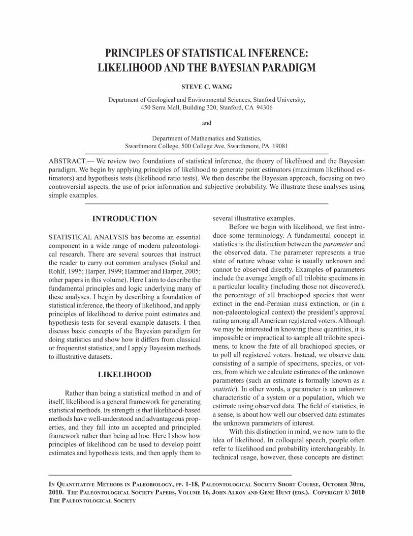
Let n denote the total number of gastropods sampled, of which x are drilled. We proceed to show that the intuitive estimate x/n is the MLE for p. To do this, we will find the likelihood function L(p) and solve for the value of p that maximizes it. As we saw above, the likelihood function L(p) is numerically equal to the probability P(x | p) of observing x drilled specimens. In this case, under some reasonable assumptions, we can model the probability of observing x drilled gastropod specimens (out of n recovered) using a Binomial distri-bution (Fig. 1.1). This distribution models the number of successful outcomes in a fixed number of indepen-dent trials, such as the number of heads in a sequence of coin flips. The binomial probability of observing x successful outcomes out of n trials is as follows:

The likelihood function is given by the same expres-sion, but considered as a function of p rather than of x (Fig. 1.2):

Note that P(x | p) is a discrete function of x because only whole number values of x are possible, whereas L(p) is a continuous function of p because p can be any real number between 0 and 1.

We now proceed to find the value of p that maxi-mizes L(p). It turns out that it is easier to maximize the logarithm of the likelihood, rather than the likelihood itself. (The log-likelihood is on a different vertical

FIGURE 1.—Probabilities and likelihoods. 1, Plot of P(x | p) assuming p = .465. Probability distribution is a discrete Binomial distribution. 2, Plot of L(p) assuming x = 138. The likelihood L(p) is numerically equal to the Binomial probability P(x | p) but expressed as a con-tinuous function of p. Triangle denotes the maximum likelihood estimate (MLE), which occurs at p = .465. 3, Plot of log L(p), the log-likelihood assuming x = 138. Triangle denotes the maximum likelihood estimate (MLE), showing that the log likelihood is maximized at the same value of p that maximizes the likelihood.

scale from the likelihood, but both functions attain a maximum at the same value of p; see Fig 1.3.) Taking the natural log of the likelihood function gives us

We want to find the value of p for which this

log L(p) = log( n!x! (n – x)! ) + x log(p) + (n – x) log(1 – p)


function is maximized. A principle of calculus is that maxima of a function usually occur where the deriva-tive is zero (i.e., where the slope of the curve is flat). Thus, we take the derivative of the log-likelihood with respect to p:

Now we set this derivative equal to zero. The MLE is the value of p at which this equality occurs, which we denote :

Solving for , we find .

Thus we have shown that the MLE is x/n = 138/297 = .465, which is indeed the common-sense estimate. That is, based on observing 138 out of 297 drilled shells in our sample, our best estimate is that .465 of shells in the entire population of all such shells at this locality would be drilled, assuming that our observed dataset is a representative random sample.

Technically, there is still some work to do. Cal-culus tells us that the point at which the derivative of a function is zero may be a maximum, minimum, or inflection point. We therefore need to verify that we have actually maximized the likelihood, rather than finding (e.g.) a minimum likelihood estimate, which would surely be undesirable. This can be done by checking the second derivative; here we omit this step for brevity. Alternately, examining a graph of the likelihood function (Fig. 1.2) makes clear that we have indeed found the maximum.

Uses and properties of maximum likelihood es-

timation.—The answer in Example 2 above matches what we would expect intuitively, so in this case the method of maximum likelihood (ML) simply tells us that the obvious answer is the correct one. While con-firming obvious answers has some value, the utility of the ML approach becomes more apparent in complex situations, where there may be no obvious answer at all. For instance, Foote (2003) uses ML to estimate the origination rate, extinction rate, and preservation rate for marine invertebrate genera in each of 77 stages

€

ˆ p

and substages spanning the Phanerozoic. Another example is Hunt (2007), who uses ML to determine the evolutionary mode (directional change, random walk, or stasis) in 250 datasets of evolving traits. Other examples in paleontology—and this is by no means an exhaustive list—include Solow (1996), Solow and Smith (1997, 2000, 2010), Wagner (1998, 2000), Sims and McConway (2003), McConway and Sims (2004), Foote (2005, 2007), Hunt (2006, 2008), Solow et al. (2006), and Wang and Everson (2007).

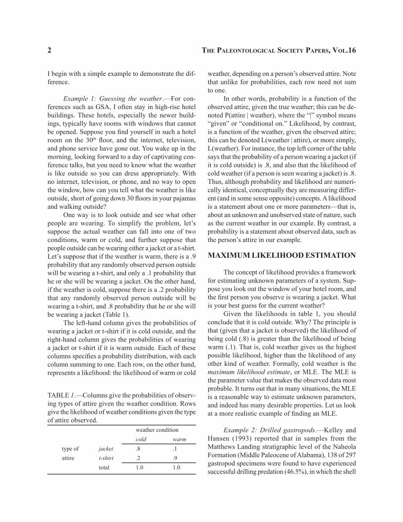
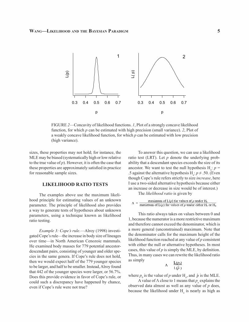
While the maximum of the likelihood function tells us the most likely value of a parameter, other as-pects of the likelihood function are informative as well. In particular, the variability of an estimate is related to the second derivative (concavity) of the likelihood function. If the likelihood function is strongly concave (Fig. 2.1), then the MLE is much more likely than are neighboring points. In other words, the MLE is much more consistent with our observed data than are other values of p. In that case, the variance or standard er-ror of

€

ˆ p is relatively small, and p can be estimated precisely. By contrast, if the likelihood function is only weakly concave (Fig. 2.1), then a relatively wide range of p values is nearly equally consistent with the observed data, and the variance of

€

ˆ p is large. In fact, one can use the shape of the likelihood function to set a confidence interval for p. A full treatment of this topic is beyond the scope of this review; see Casella and Berger (2002, chapter 7) for details.

In addition to being intuitively appealing, maxi-mum likelihood estimates have many useful statisti-cal properties (Casella and Berger, 2002, chapter 7). Under some reasonable conditions on the probability model, it can be shown that MLEs have the following asymptotic properties:

1) Unbiasedness: the expected value of the MLE is equal to the true parameter value2) Efficiency: the MLE has the smallest pos-

sible variance among unbiased estimators of the parameter

3) Normality: the sampling distribution of the MLE is Normal (Gaussian)

4) Consistency: the MLE becomes arbitrarily close to the true parameter value

It is important to emphasize that these are asymp-totic properties; that is, they hold as the sample size increases to infinity. Of course, no real dataset ever has an infinite number of observations. For finite sample

d

dp log L(p) = 0 +

xp –

n – x1 – p

€

ˆ p


sizes, these properties may not hold; for instance, the MLE may be biased (systematically high or low relative to the true value of p). However, it is often the case that these properties are approximately satisfied in practice for reasonable sample sizes.

lIKelIhood ratIo tests

The examples above use the maximum likeli-hood principle for estimating values of an unknown parameter. The principle of likelihood also provides a way to generate tests of hypotheses about unknown parameters, using a technique known as likelihood ratio testing.

Example 3: Cope’s rule.—Alroy (1998) investi-gated Cope’s rule—the increase in body size of lineages over time—in North American Cenozoic mammals. He examined body masses for 779 potential ancestor-descendant pairs, consisting of younger and older spe-cies in the same genera. If Cope’s rule does not hold, then we would expect half of the 779 younger species to be larger, and half to be smaller. Instead, Alroy found that 442 of the younger species were larger, or 56.7%. Does this provide evidence in favor of Cope’s rule, or could such a discrepancy have happened by chance, even if Cope’s rule were not true?

0.3 0.4 0.5 0.6 0.7

p

L(p)

1

0.3 0.4 0.5 0.6 0.7

p

L( p

)

2

FIGURE 2—Concavity of likelihood functions. 1, Plot of a strongly concave likelihood function, for which p can be estimated with high precision (small variance). 2, Plot of a weakly concave likelihood function, for which p can be estimated with low precision (high variance).

To answer this question, we can use a likelihood ratio test (LRT). Let p denote the underlying prob-ability that a descendant species exceeds the size of its ancestor. We want to test the null hypothesis Ho: p = .5 against the alternative hypothesis Ha: p ≠ .50. (Even though Cope’s rule refers strictly to size increase, here I use a two-sided alternative hypothesis because either an increase or decrease in size would be of interest.)

The likelihood ratio is given by

This ratio always takes on values between 0 and 1, because the numerator is a more restrictive maximum and therefore cannot exceed the denominator, which is a more general (unconstrained) maximum. Note that the denominator calls for the maximum height of the likelihood function reached at any value of p consistent with either the null or alternative hypotheses. In most cases, this value of p is simply the MLE, by definition. Thus, in many cases we can rewrite the likelihood ratio as simply

where p0 is the value of p under Ho, and

€

ˆ p is the MLE.A value of Λ close to 1 means that po explains the

observed data almost as well as any value of p does, because the likelihood under Ho is nearly as high as


the likelihood could ever possibly be. In that case, we do not reject the null hypothesis. A small value of Λ (close to 0), on the other hand, implies that Ho explains the observed data much more poorly than the best pos-sible value of p does. In that case, we reject the null hypothesis; there are other hypotheses that explain the observed data much better. A natural question is, how small is a “small” value of Λ?

To answer this question, we use –2 log Λ as our test statistic, rather than Λ itself. It can be shown that under some reasonable conditions, if the null hypothesis is true, then –2 log Λ follows a chi-square distribution (Casella and Berger 2002, chapter 8). The number of degrees of freedom is equal to the difference in the number of free parameters specified under Ho, and the number under Ho and Ha taken together. In our ex-ample, under Ho there are no free parameters (because p is constrained to be .5), and under Ho and Ha taken together there is one free parameter (because p can be any real number between 0 and 1), so we have 1 – 0 = 1 degree of freedom.

Let x denote the number of pairs (out of the n pairs observed) in which the descendant species exceeds the size of its potential ancestor. We can model the prob-ability of observing x descendant size increases using a Binomial distribution with parameter p. The likelihood function is therefore

Under the null hypothesis we have p0 = .5 and

€

ˆ p = x /n as derived in Example 2, which here equals 442/779 = .567. Thus the likelihood ratio is

=.000827

This value is small—much closer to zero than to one—meaning that Ho does not explain the data nearly as well as the MLE explains the data. To formalize this conclusion, we calculate the test statistic –2 log Λ, which equals –2 log(.000827) = 14.2. Under H0 the test

statistic follows a chi-square distribution with (1 – 0) = 1 degree of freedom. The p-value associated with a chi-square value of 14.2 is .0002, so we reject H0 and conclude that this dataset provides strong evidence sup-porting p ≠ .5 (and specifically p > .5), implying that Cope’s rule holds for North American fossil mammals.

Uses and properties of likelihood ratio tests.—For the dataset in Example 3, several standard tests could have been used to test for Cope’s rule, such as a z-test, chi-square test, or G-test. In fact, many standard tests can be derived as likelihood ratio tests, or are approximately equivalent to LRTs. As with maximum likelihood estimation, the value of the LRT framework is that it can be applied to situations for which there are no existing standard methods. For instance, Wang and Everson (2007) use LRTs to test for multiple extinc-tion pulses based on stratigraphic range data. Another example is Sims and McConway (2003), who use LRTs to test for heterogeneity in diversification rates in angiosperms. For other examples in paleontology, see the references given above in the section on “Uses and properties of maximum likelihood estimation.”

As with maximum likelihood estimation, likeli-hood ratio tests have optimality properties under certain conditions. It can be shown that in some situations, the LRT is the most powerful test for a given α level (Type I error rate). That is, for a given false positive error rate, the LRT is better able to detect departures from the null hypothesis than is any other test (Casella and Berger 2002, chapter 8.)

the bayesIan ParadIgM

In the past few decades, the Bayesian approach to statistics has become increasingly popular. Here we present the Bayesian approach and describe how it dif-fers from classical or “frequentist” statistics, focusing on two particularly controversial points: the use of prior information and subjective probability.

PrIor belIeF

In analyzing a dataset, should we use prior knowledge obtained external to the dataset itself? The Bayesian approach allows scientists to incorporate such prior knowledge in the results of an analysis. Here are three examples in which prior knowledge might be at


odds with the actual experimental results.

Example 4.—You are a pollster carrying out an opinion poll to assess how potential voters feel about the job the president is doing. Contemporaneous polls by other organizations have found the president’s approval rating at approximately 55%. Your poll, however, finds only 41% approving of the president. Given what other polls are reporting, this result seems unexpectedly low. Perhaps, you suspect, your sample happened to be unrepresentative of potential voters as a whole, just by random chance. To get the best estimate of the president’s approval rating, should you therefore adjust your results upwards to account for this external knowledge, and report the approval rating as being higher than 41%—say, averaging 41% and 55% to arrive at a figure of 48%?

Example 5.—You are carrying out a clinical trial of a new cholesterol-lowering drug for a pharmaceutical company. From previous clinical trials and from similar drugs in this class, your expectation is that this drug will reduce cholesterol by 15 points. However, your clinical trial finds that on average, the new drug reduces cholesterol by only 5 points. You speculate that the subjects in your study, for whatever reason, responded less well to the drug than most patients would. Is it proper to incorporate your prior knowledge and report that the drug is expected to lower cholesterol by, say, 10 points in its intended population?

Example 6.—You are a student taking a class. On the final exam, you score a 96%, which should be a solid A grade. However, the professor knows that you have had trouble in two previous classes in the same subject, earning a C and C+. The professor suspects that you might have gotten lucky on the final exam—perhaps the questions on the exam just happened to match the topics you studied, or by chance you guessed correctly on some questions you didn’t really know. To better reflect your knowledge of the material, should the professor discount your score and give you a B+ on the final exam instead of an A?

Often people find it unscientific or even unethical to incorporate prior knowledge in these scenarios. On the other hand, one might argue that there is always prior knowledge in scientific problems. After all, we don’t think (non-avian) dinosaurs went extinct last

Tuesday, or that smoking increases longevity; any stud-ies that came to such conclusions would immediately be found dubious. Why should we not incorporate such knowledge into the scientific process? The Bayesian approach allows, even encourages, scientists to specify and incorporate their prior knowledge, and this is one reason that it has been controversial. Below (in Ex-ample 10) we will see a situation in which it may be more reasonable to incorporate prior knowledge into an analysis.

subJectIve ProbabIlIty

Another aspect of the Bayesian paradigm that has been controversial is its use of a subjective definition of probability. Before examining this subjective defi-nition, we begin by discussing the classical definition of probability.

The frequentist definition of probability.—What does it mean to say that when one flips a coin, the probability of getting a heads is ½? There are several ways of defining the concept of probability. The most commonly used definition in traditional statistics is the classical or frequentist definition, so-called because it is based on long-run relative frequencies. According to this definition, when we say that the probability of flipping heads is ½, we mean that the proportion of flips landing heads approaches ½ in an infinitely long sequence of repeated flips. In other words, ½ is the

limit of the fraction as n goes to infinity. Although this definition seems simple enough, there are some complications that arise in applying the defini-tion. First, this definition is an empirical one; to use it to assign probabilities to events, we must (if we are to follow the definition strictly) repeat a series of events an infinite number of times. Clearly, this is impossible. Second, and more importantly for our purposes, this definition can be applied only to events that can be, at least in theory, repeated an infinite number of times. It cannot be applied to events that are unique or non-repeatable. Consider the following probabilities:

Example 7.—The New York Yankees won the World Series in the 2009 major league baseball sea-son. What is the probability that they will repeat as champions in 2010?


Example 8.—There are currently at least two high-profile female politicians who have run or may be considering running for the President of the United States. What is the probability that the U.S. will elect its first female president in 2012?

Example 9.—Arizona and New Mexico are both large states (in terms of land area) in the southwestern United States. Off the top of my head I’m not sure which one is larger—perhaps New Mexico. What is the probability that New Mexico is in fact larger than Arizona?

None of these events is infinitely repeatable, even in theory, in the way that a coin flip is; all are unique. The 2010 World Series is held only once, as is the 2012 U.S. election. The sizes of Arizona and New Mexico are not even future events; they are just facts. Nonetheless, it may seem reasonable to use the term “probability” in these contexts, because these events are uncertain. This uncertainty is the basis of the subjective definition of probability used in Bayesian statistics. Unlike the frequentist definition of probability, which is a measure of randomness, subjective probability is a measure of uncertainty or degree of belief. Any event that is uncertain can therefore be assigned a probability, whether it is repeatable or not. Different people may as-sign different subjective probabilities to the same event, as your measure of uncertainty may differ from mine (for instance, you may be from New Mexico and know exactly how large it is). Regardless of one’s degree of belief, however, the Bayesian paradigm provides a framework in which one can update one’s initial (prior) belief in light of newly observed information.

Although the use of prior information has been the object of some controversy, in my opinion it is the use of subjective probability that is the most important aspect—or rather, benefit—of the Bayesian approach. In many situations, subjective probability provides a more straightforward interpretation of the results of an analysis than a frequentist interpretation does. For instance, a frequentist might report in Example 2 that a 95% confidence interval for p, the proportion of drilled gastropods is (42%, 51%). It is tempting to interpret this interval as meaning that there is a 95% probability that p is between 42% and 51%. Not only is this interpretation incorrect, however, it is not even a valid use of the concept of probability, according to the frequentist definition. In this situation, p is a fixed

(but unknown) quantity, and the confidence limits 42% and 51% are fixed as well. With no random or stochastically varying quantities present, the frequentist concept of probability is simply inapplicable. It does not make sense to ask what proportion of the time p lies between 42% and 51%: either it is between 42% and 51%, or it is not. (Such a question would be analogous to asking for the probability that 2 is between 1 and 3, which is nonsensical.) All we can say in this situation is that our method of finding confidence intervals, if applied to an infinite number of samples, would yield an interval—not necessarily (42%, 51%)—that captures p 95% of the time.

On the other hand, the Bayesian equivalent of a confidence interval (termed a credible interval) allows the straightforward interpretation that there is a 95% probability that p lies between 42% and 51%. Using the subjective definition of probability, this interpreta-tion is valid because even though p is not random, it is uncertain. The fact that a Bayesian approach allows this natural inference is an important advantage compared to the more indirect frequentist interpretation, which permits conclusions only about the long-run success rate of the confidence interval procedure rather than about the particular interval (42%, 51%) itself. In Examples 10 and 11 below, we calculate examples of Bayesian credible intervals.

eXaMPle: returnIng lost Wallets

Example 10.—Here we carry out a simple ex-ample of a Bayesian analysis, which should clarify the distinction between the frequentist and Bayesian approaches. Suppose you are on vacation in an unfa-miliar city. As you are walking down the street, you come across a wallet on the ground that someone has apparently dropped, containing ID, family photos, credit cards, and some cash. What do you do with it? You see a police officer on patrol; aren’t they supposed to be able to help in situations like this? You give the wallet to the officer and ask him or her to return it to its rightful owner. What will the officer do? Some readers may suspect that the officer will be tempted to keep some of the money. What is the probability p that the officer will steal some of the cash in the wallet before attempting returning it?

The ABC news program PrimeTime (ABC News,


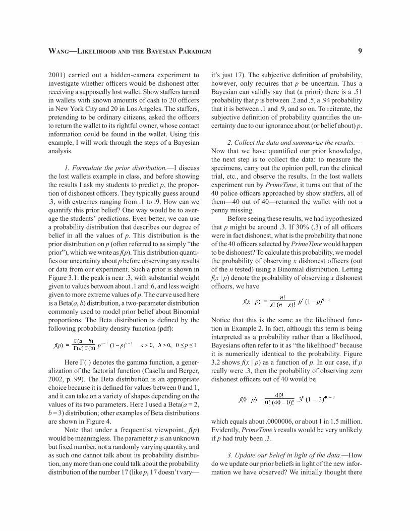
2001) carried out a hidden-camera experiment to investigate whether officers would be dishonest after receiving a supposedly lost wallet. Show staffers turned in wallets with known amounts of cash to 20 officers in New York City and 20 in Los Angeles. The staffers, pretending to be ordinary citizens, asked the officers to return the wallet to its rightful owner, whose contact information could be found in the wallet. Using this example, I will work through the steps of a Bayesian analysis.

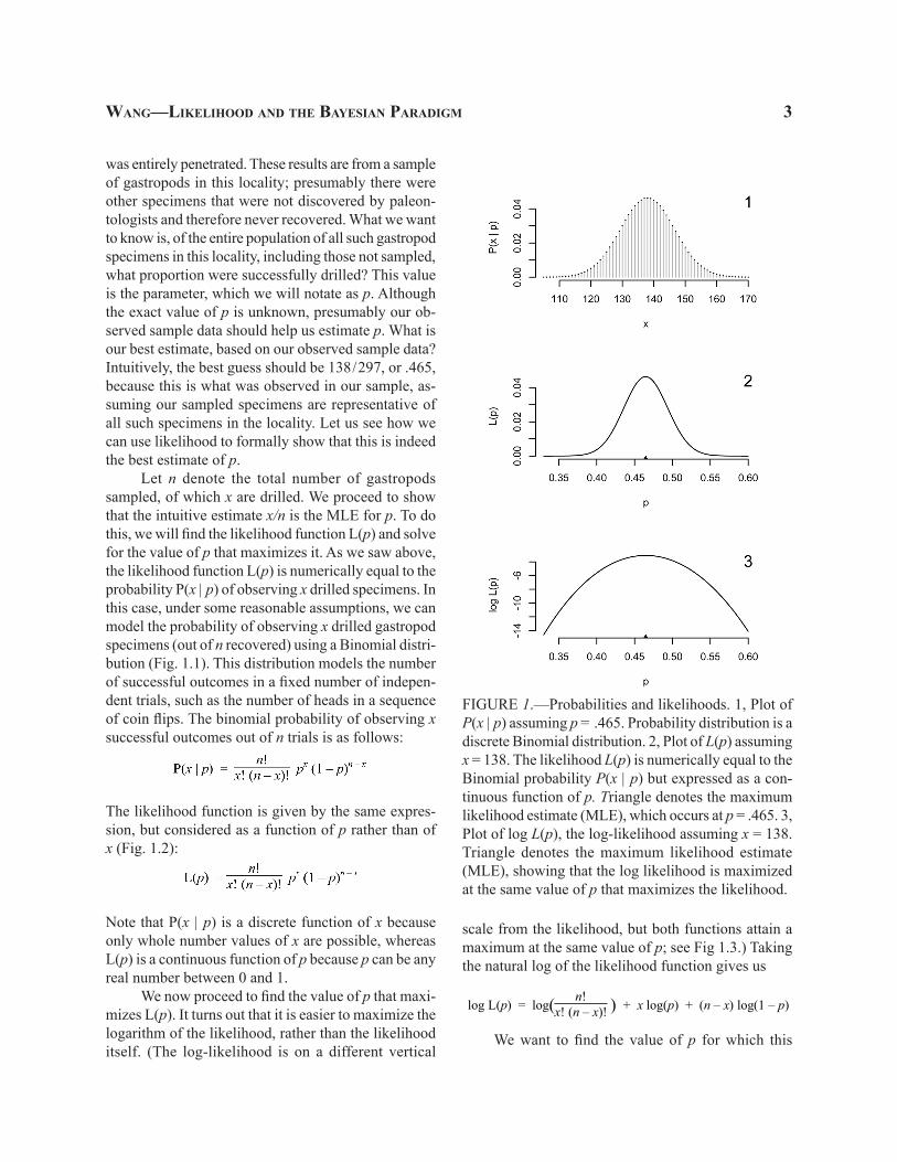
1. Formulate the prior distribution.—I discuss the lost wallets example in class, and before showing the results I ask my students to predict p, the propor-tion of dishonest officers. They typically guess around .3, with extremes ranging from .1 to .9. How can we quantify this prior belief? One way would be to aver-age the students’ predictions. Even better, we can use a probability distribution that describes our degree of belief in all the values of p. This distribution is the prior distribution on p (often referred to as simply “the prior”), which we write as f(p). This distribution quanti-fies our uncertainty about p before observing any results or data from our experiment. Such a prior is shown in Figure 3.1: the peak is near .3, with substantial weight given to values between about .1 and .6, and less weight given to more extreme values of p. The curve used here is a Beta(a, b) distribution, a two-parameter distribution commonly used to model prior belief about Binomial proportions. The Beta distribution is defined by the following probability density function (pdf):

Here Γ( ) denotes the gamma function, a gener-alization of the factorial function (Casella and Berger, 2002, p. 99). The Beta distribution is an appropriate choice because it is defined for values between 0 and 1, and it can take on a variety of shapes depending on the values of its two parameters. Here I used a Beta(a = 2, b = 3) distribution; other examples of Beta distributions are shown in Figure 4.

Note that under a frequentist viewpoint, f(p) would be meaningless. The parameter p is an unknown but fixed number, not a randomly varying quantity, and as such one cannot talk about its probability distribu-tion, any more than one could talk about the probability distribution of the number 17 (like p, 17 doesn’t vary—

it’s just 17). The subjective definition of probability, however, only requires that p be uncertain. Thus a Bayesian can validly say that (a priori) there is a .51 probability that p is between .2 and .5, a .94 probability that it is between .1 and .9, and so on. To reiterate, the subjective definition of probability quantifies the un-certainty due to our ignorance about (or belief about) p.

2. Collect the data and summarize the results.—Now that we have quantified our prior knowledge, the next step is to collect the data: to measure the specimens, carry out the opinion poll, run the clinical trial, etc., and observe the results. In the lost wallets experiment run by PrimeTime, it turns out that of the 40 police officers approached by show staffers, all of them—40 out of 40—returned the wallet with not a penny missing.

Before seeing these results, we had hypothesized that p might be around .3. If 30% (.3) of all officers were in fact dishonest, what is the probability that none of the 40 officers selected by PrimeTime would happen to be dishonest? To calculate this probability, we model the probability of observing x dishonest officers (out of the n tested) using a Binomial distribution. Letting f(x | p) denote the probability of observing x dishonest officers, we have

Notice that this is the same as the likelihood func-tion in Example 2. In fact, although this term is being interpreted as a probability rather than a likelihood, Bayesians often refer to it as “the likelihood” because it is numerically identical to the probability. Figure 3.2 shows f(x | p) as a function of p. In our case, if p really were .3, then the probability of observing zero dishonest officers out of 40 would be

which equals about .0000006, or about 1 in 1.5 million. Evidently, PrimeTime’s results would be very unlikely if p had truly been .3.

3. Update our belief in light of the data.—How do we update our prior beliefs in light of the new infor-mation we have observed? We initially thought there


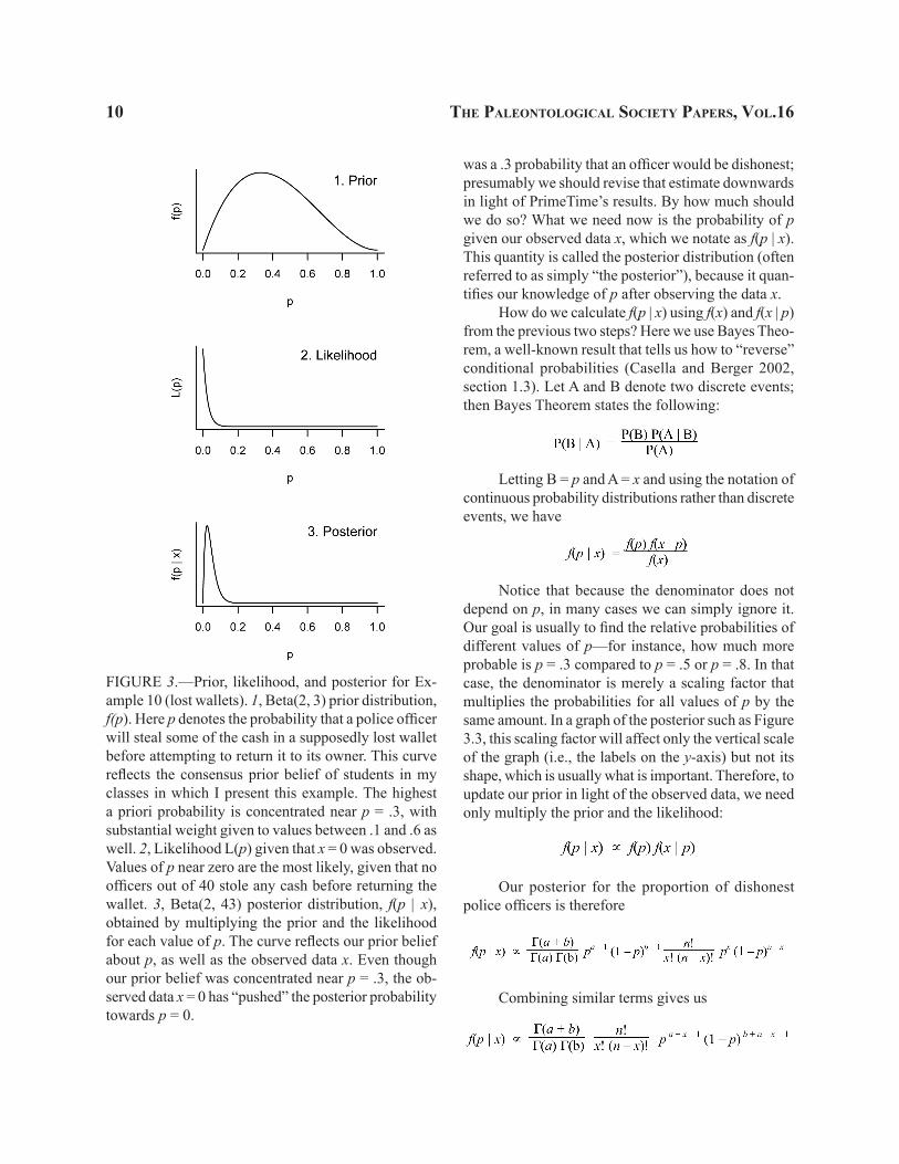
FIGURE 3.—Prior, likelihood, and posterior for Ex-ample 10 (lost wallets). 1, Beta(2, 3) prior distribution, f(p). Here p denotes the probability that a police officer will steal some of the cash in a supposedly lost wallet before attempting to return it to its owner. This curve reflects the consensus prior belief of students in my classes in which I present this example. The highest a priori probability is concentrated near p = .3, with substantial weight given to values between .1 and .6 as well. 2, Likelihood L(p) given that x = 0 was observed. Values of p near zero are the most likely, given that no officers out of 40 stole any cash before returning the wallet. 3, Beta(2, 43) posterior distribution, f(p | x), obtained by multiplying the prior and the likelihood for each value of p. The curve reflects our prior belief about p, as well as the observed data x. Even though our prior belief was concentrated near p = .3, the ob-served data x = 0 has “pushed” the posterior probability towards p = 0.

was a .3 probability that an officer would be dishonest; presumably we should revise that estimate downwards in light of PrimeTime’s results. By how much should we do so? What we need now is the probability of p given our observed data x, which we notate as f(p | x). This quantity is called the posterior distribution (often referred to as simply “the posterior”), because it quan-tifies our knowledge of p after observing the data x.

How do we calculate f(p | x) using f(x) and f(x | p) from the previous two steps? Here we use Bayes Theo-rem, a well-known result that tells us how to “reverse” conditional probabilities (Casella and Berger 2002, section 1.3). Let A and B denote two discrete events; then Bayes Theorem states the following:

Letting B = p and A = x and using the notation of continuous probability distributions rather than discrete events, we have

Notice that because the denominator does not depend on p, in many cases we can simply ignore it. Our goal is usually to find the relative probabilities of different values of p—for instance, how much more probable is p = .3 compared to p = .5 or p = .8. In that case, the denominator is merely a scaling factor that multiplies the probabilities for all values of p by the same amount. In a graph of the posterior such as Figure 3.3, this scaling factor will affect only the vertical scale of the graph (i.e., the labels on the y-axis) but not its shape, which is usually what is important. Therefore, to update our prior in light of the observed data, we need only multiply the prior and the likelihood:

Our posterior for the proportion of dishonest police officers is therefore

Combining similar terms gives us


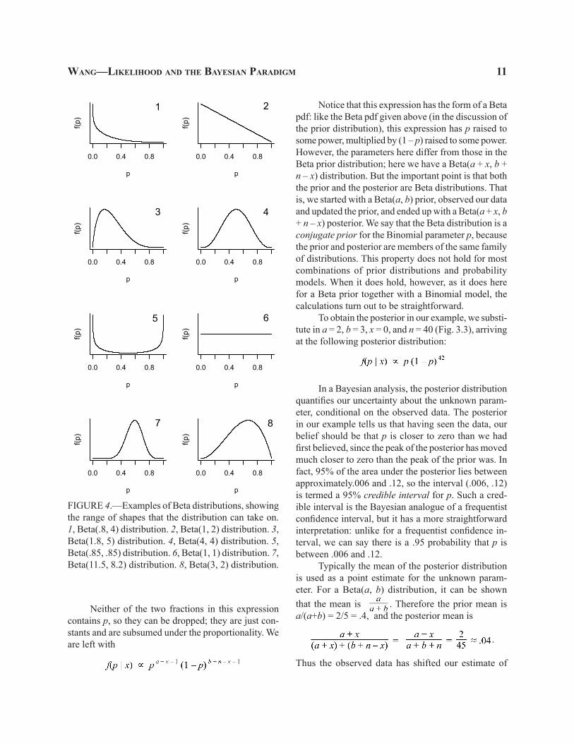
FIGURE 4.—Examples of Beta distributions, showing the range of shapes that the distribution can take on. 1, Beta(.8, 4) distribution. 2, Beta(1, 2) distribution. 3, Beta(1.8, 5) distribution. 4, Beta(4, 4) distribution. 5, Beta(.85, .85) distribution. 6, Beta(1, 1) distribution. 7, Beta(11.5, 8.2) distribution. 8, Beta(3, 2) distribution.

Neither of the two fractions in this expression contains p, so they can be dropped; they are just con-stants and are subsumed under the proportionality. We are left with

Notice that this expression has the form of a Beta pdf: like the Beta pdf given above (in the discussion of the prior distribution), this expression has p raised to some power, multiplied by (1 – p) raised to some power. However, the parameters here differ from those in the Beta prior distribution; here we have a Beta(a + x, b + n – x) distribution. But the important point is that both the prior and the posterior are Beta distributions. That is, we started with a Beta(a, b) prior, observed our data and updated the prior, and ended up with a Beta(a + x, b + n – x) posterior. We say that the Beta distribution is a conjugate prior for the Binomial parameter p, because the prior and posterior are members of the same family of distributions. This property does not hold for most combinations of prior distributions and probability models. When it does hold, however, as it does here for a Beta prior together with a Binomial model, the calculations turn out to be straightforward.

To obtain the posterior in our example, we substi-tute in a = 2, b = 3, x = 0, and n = 40 (Fig. 3.3), arriving at the following posterior distribution:

In a Bayesian analysis, the posterior distribution quantifies our uncertainty about the unknown param-eter, conditional on the observed data. The posterior in our example tells us that having seen the data, our belief should be that p is closer to zero than we had first believed, since the peak of the posterior has moved much closer to zero than the peak of the prior was. In fact, 95% of the area under the posterior lies between approximately.006 and .12, so the interval (.006, .12) is termed a 95% credible interval for p. Such a cred-ible interval is the Bayesian analogue of a frequentist confidence interval, but it has a more straightforward interpretation: unlike for a frequentist confidence in-terval, we can say there is a .95 probability that p is between .006 and .12.

Typically the mean of the posterior distribution is used as a point estimate for the unknown param-eter. For a Beta(a, b) distribution, it can be shown that the mean is . Therefore the prior mean is a/(a+b) = 2/5 = .4, and the posterior mean is

.

Thus the observed data has shifted our estimate of

0.0 0.4 0.8

p

f(p)

1

0.0 0.4 0.8

pf(p

)

2

0.0 0.4 0.8

p

f(p)

3

0.0 0.4 0.8

p

f(p)

4

0.0 0.4 0.8

p

f(p)

5

0.0 0.4 0.8

p

f(p)

6

0.0 0.4 0.8

p

f(p)

7

0.0 0.4 0.8

p

f(p)

8


p closer to zero by an order of magnitude. Note that

the posterior mean incorporates the prior mean , as well as the maximum likelihood estimate from Example 2. In fact, we can rewrite the posterior mean

as . In this form, we can see that the posterior mean is dominated by the prior mean when the sample size is small, but approaches the MLE as the sample size increases. That is, when there is little data, the posterior mean primarily reflects our prior belief. But when the sample size is large, the posterior mean is weighted towards the MLE, letting the data speak for themselves and diminishing the influence of the prior.

dIscussIon: lost Wallets

Incorporating prior knowledge.—In the lost wal-lets example, it seems reasonable to incorporate prior knowledge at least to some extent. A strictly frequen-tist analysis would report that the best estimate is the MLE,

€

ˆ p = 0. But if we have a fairly strong prior belief that p ≠ 0, is it really sensible to report an estimate of

€

ˆ p = 0? A Bayesian would argue that the posterior mean,

€

ˆ p = .04, is a more realistic estimate. In fact, one could argue that frequentists sometimes incorporate prior belief as well. If a frequentist observes experimental results that contradict his or her knowledge, he or she may decide to run the experiment longer than originally planned in order to collect more data, or even throw out the discrepant results entirely and begin anew. Such actions also constitute accounting for prior information, but in a haphazard way. The strength of the Bayesian approach is that it provides a coherent and principled way of incorporating such information.

Noninformative priors.— Most people have some prior belief about the honesty of police officers that may have been shaped by television dramas, real-life trials and scandals, and other information. But what if we had no prior belief about p in some situation, or we were unwilling to specify our prior belief? In that case, we could use a flat or uniform prior (Figure 4.6), giving equal prior weight to all values of p. One might prefer such an approach because it is noninformative about p — it does not favor any particular outcome a priori. However, a Bayesian might argue that there is always some prior belief; surely not every value of p

between 0 and 1 is equally probable, so our analysis should not pretend that is the case.

On the other hand, one might favor the Bayesian interpretation of probability, or the ability of Bayesian models to account for multiple sources of uncertainty, yet seek to minimize the effect of the prior on the analy-sis. This has led to the development of objective Bayes methods, which attempt to determine prior distributions through formal rules rather than subjective judgment. Accomplishing this goal is not as simple as merely us-ing a uniform prior. Note, for instance, that a prior that is uniform on one measurement scale (e.g., kilograms) may not be uniform when the data are transformed (e.g., log kilograms). One solution to this issue is the Jeffreys prior (Jeffreys, 1961), an objective prior that is invariant to changes in parametrization. The broader question of how to select priors by objective rules is an active research area; see Kass and Wasserman (1996) and Berger (2006) for overviews. The growth of ob-jective Bayes methods is an important development because it expands the audience for Bayesian modeling to those who want to take advantage of its flexibility, but aren’t necessarily interested in incorporating prior information.

Connections with frequentist inference.—What happens to the posterior if we use a uniform prior? In Step 3 above, we saw that f(p | x) ∝ f(p) f(x | p), with the latter term on the right-hand side being numerically equal to the likelihood. With a uniform prior, we have f(p) ∝ 1, so that the prior has essentially no effect on the posterior. This implies that f(p | x) ∝ f(x | p)—in other words, the posterior is simply the likelihood, and the MLE is equivalent to the posterior mode. What a non-uniform prior does is to give varying weights to the likelihood in different regions of the parameter space. The posterior, in this sense, is a weighted likelihood, in which the weights reflect prior belief. Seen from this viewpoint, the Bayesian approach is not so dif-ferent from the frequentist likelihood-based approach. Bayesians use a different conception of probability, and they typically look at the posterior mean rather than the mode, but both frequentist and Bayesian approaches are based on the likelihood function.

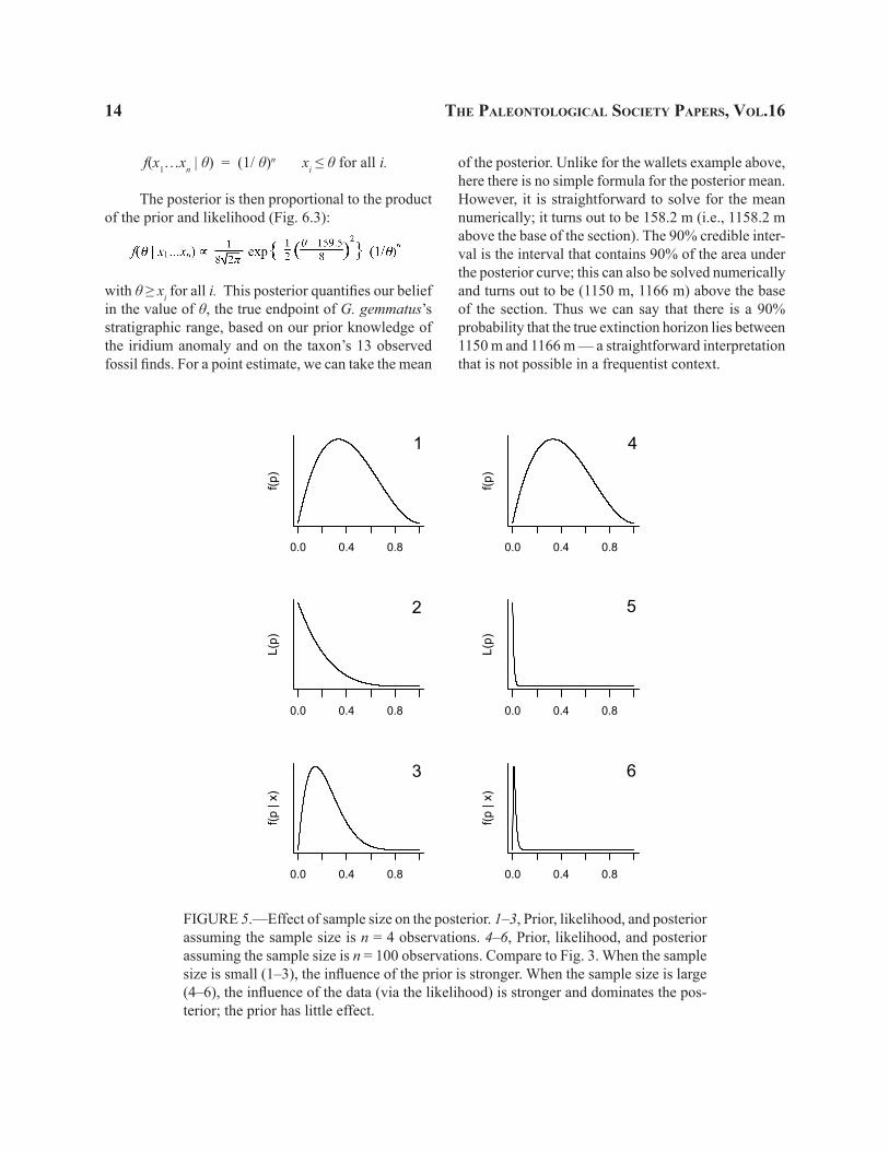
Dependence of the posterior on sample size.—The shape of the posterior depends not only on the prior and the observed data, but also on the sample size. Figure 5.1 shows the posterior that would have


resulted if we had observed the same result (0 dishonest officers) but with a sample size of n = 4 instead of n = 40, and Figure 5.2 shows the posterior if n had been 100. In the former case, the posterior is more heavily influenced by the prior; the relative lack of empirical information means our prior belief is relatively little affected by the data. In the latter case, the large amount of empirical information overwhelms our prior, and the posterior primarily reflects the observed data.

eXaMPle: late cretaceous aM-MonIte eXtInctIon

Example 11.—We close with an example of a Bayesian analysis of paleontological data. Although Bayesian modeling in paleontology dates back at least to Strauss and Sadler (1989), such analyses have not yet become commonplace outside of phylogeny reconstruction. One example was given by Wang et al. (2006), who use Bayesian methods to infer extinc-tion levels in a 22-parameter model of a Late Permian food web. Another example was described by Han-nisdal (2007), who analyzed phenotypic evolution in foraminifera, using a Bayesian model to control for uncertainty arising from several geological variables and measurement error. A third example was given by Puolamäki et al. (2006), who used a Bayesian model to determine the temporal ordering of fossil sites given data on the taxa occurring in each site. These examples highlight an additional strength of Bayesian methods: they are well adapted to high-dimensional problems in which one must account for numerous sources of uncertainty in a coherent way.

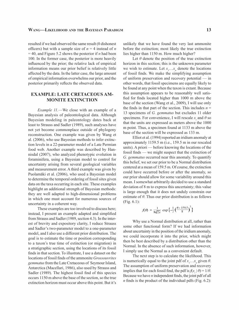
These examples are too involved to discuss here; instead, I present an example adapted and simplified from Strauss and Sadler (1989, section 4.3). In the inter-est of brevity and expository clarity, I reduce Strauss and Sadler’s two-parameter model to a one-parameter model, and I also use a different prior distribution. The goal is to estimate the time or position corresponding to a taxon’s true time of extinction (or migration) in a stratigraphic section, using the locations of its fossil finds in that section. To illustrate, I use a dataset on the locations of fossil finds of the ammonite Grossouvrites gemmatus from the Late Cretaceous of Seymour Island, Antarctica (Macellari, 1986), also used by Strauss and Sadler (1989). The highest fossil find of this species occurs 1150 m above the base of the section, so the true extinction horizon must occur above this point. But it’s

unlikely that we have found the very last ammonite before the extinction; most likely the true extinction lies higher than 1150 m. How much higher?

Let θ denote the position of the true extinction horizon in this section; this is the unknown parameter we wish to estimate. Let x1…xn denote the locations of fossil finds. We make the simplifying assumption of uniform preservation and recovery potential — in other words, that fossil specimens are equally likely to be found at any point when the taxon is extant. Because this assumption appears to be reasonably well satis-fied for finds located higher than 1000 m above the base of the section (Wang et al., 2009), I will use only the finds in that part of the section. This includes n = 13 specimens of G. gemmatus but excludes 11 older specimens. For convenience, I will rescale xi and θ so that the units are expressed as meters above the 1000 m point. Thus, a specimen found at 1133 m above the base of the section will be expressed as 133 m.

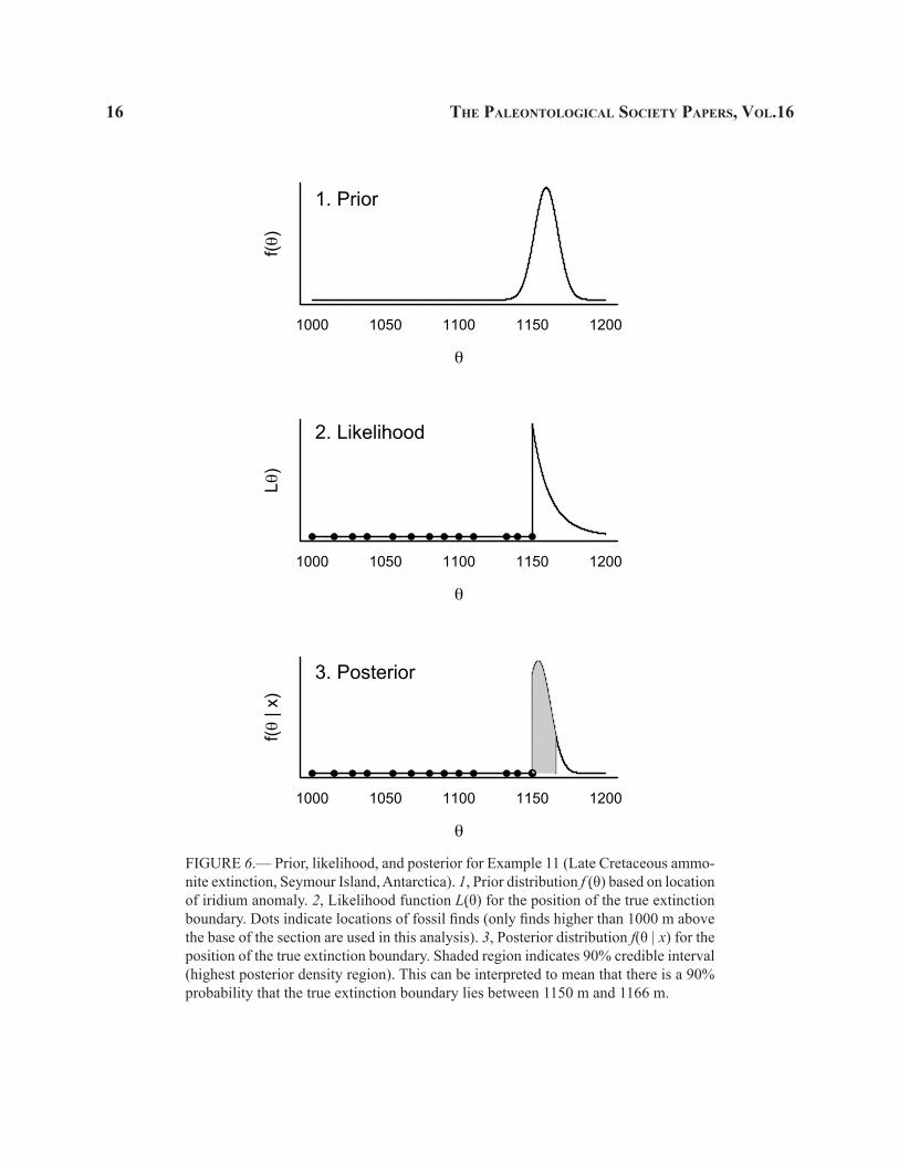
Elliot et al. (1994) reported an iridium anomaly at approximately 1159.5 m (i.e., 159.5 m in our rescaled units). A priori — before knowing the locations of the fossil finds — we might suspect that the extinction of G. gemmatus occurred near this anomaly. To quantify this belief, we set our prior to be a Normal distribution centered at a mean of 159.5 m. Of course, the extinction could have occurred before or after the anomaly, so our prior should allow for some variability around this mean. I somewhat arbitrarily decided to use a standard deviation of 8 m to express this uncertainty; this value is large enough that it does not unduly constrain our estimate of θ. Thus our prior distribution is as follows (Fig. 6.1):

Why use a Normal distribution at all, rather than some other functional form? If we had information about uncertainty in the position of the iridium anomaly, we could incorporate it into the prior, which might then be best described by a distribution other than the Normal. In the absence of such information, however, I simply use the Normal as a convenient default.

The next step is to calculate the likelihood. This is numerically equal to the joint pdf of x1…xn given θ. The assumption of uniform preservation and recovery implies that for each fossil find, the pdf is f(xi | θ) = 1/θ. Because we have n independent finds, the joint pdf of all n finds is the product of the individual pdfs (Fig. 6.2):


f(x1…xn | θ) = (1/ θ)n xi ≤ θ for all i.

The posterior is then proportional to the product of the prior and likelihood (Fig. 6.3):

with θ ≥ xi for all i. This posterior quantifies our belief in the value of θ, the true endpoint of G. gemmatus’s stratigraphic range, based on our prior knowledge of the iridium anomaly and on the taxon’s 13 observed fossil finds. For a point estimate, we can take the mean

of the posterior. Unlike for the wallets example above, here there is no simple formula for the posterior mean. However, it is straightforward to solve for the mean numerically; it turns out to be 158.2 m (i.e., 1158.2 m above the base of the section). The 90% credible inter-val is the interval that contains 90% of the area under the posterior curve; this can also be solved numerically and turns out to be (1150 m, 1166 m) above the base of the section. Thus we can say that there is a 90% probability that the true extinction horizon lies between 1150 m and 1166 m — a straightforward interpretation that is not possible in a frequentist context.

0.0 0.4 0.8

p

f(p)

1

0.0 0.4 0.8

p

L(p)

2

0.0 0.4 0.8

f(p |

x)

3

0.0 0.4 0.8

p

f(p)

4

0.0 0.4 0.8

p

L(p)

5

0.0 0.4 0.8

f(p |

x)

6

FIGURE 5.—Effect of sample size on the posterior. 1–3, Prior, likelihood, and posterior assuming the sample size is n = 4 observations. 4–6, Prior, likelihood, and posterior assuming the sample size is n = 100 observations. Compare to Fig. 3. When the sample size is small (1–3), the influence of the prior is stronger. When the sample size is large (4–6), the influence of the data (via the likelihood) is stronger and dominates the pos-terior; the prior has little effect.


Note that any interval containing 90% of the area under the curve is a 90% credible interval; such intervals are not unique. For example, we could take the interval that contains the middle 90% of the area under the curve, with 5% lying outside the interval on either side (the equal-tail interval). Another option is to take the interval corresponding to the values of θ for which the posterior density is highest (the highest posterior density interval). Here I used the latter option, as it results in the shortest possible interval.

More coMPleX Models: MarKov chaIn Monte carlo

In Example 10, the Beta distribution was the conjugate prior corresponding to the Binomial model. This fact is mathematically convenient: once we know that we have a conjugate prior, we need not carry out the actual multiplication of f(p) and f(x | p) to obtain the posterior; we need only update the parameters of f(p) to arrive at f(p | x). Furthermore, the fact that we have a conjugate prior means that we can calculate the actual value of the posterior (not just a value propor-tional to the posterior) without having to evaluate the scaling factor f(x), which is often a difficult calculation. In addition to the Beta/Binomial case presented here, there are other situations in which conjugate priors ex-ist: Normal priors for Normal models, Gamma priors for Poisson and Exponential models, Dirichlet priors for Multinomial models, etc. (Gelman et al., 2003). In cases where there is no conjugate prior, the form of the posterior distribution can be messy, making it difficult to find the posterior mean or other summary statistics. In such cases, there is typically no closed-form solu-tion for the posterior mean, and it becomes necessary to use numerical techniques; this was the case in Ex-ample 11. That example had only one parameter, so it was not difficult to solve for the posterior mean and credible interval using simple numerical techniques. In more complex situations, such as the 22-parameter problem of Wang et al. (2006), more sophisticated numerical techniques are necessary. Commonly used are Markov Chain Monte Carlo (MCMC) methods such as the Gibbs Sampler (Geman and Geman 1984) and the Metropolis-Hastings algorithm (Metropolis et al. 1953, Hastings 1970). These iterative algorithms are computationally intensive, but the growth of fast computing power in the last two decades has made

such techniques more practical, contributing to the popularity of Bayesian methods. Here I briefly describe conceptually how MCMC methods work; see Gelfand and Smith (1990), Gelman et al. (2003), and Manly (2006) for details. For simplicity, my explanation is in the context of a one-parameter problem, but keep in mind that these methods generalize to and are especially useful for multi-parameter problems.

Our goal is to estimate quantities associated with the posterior distribution, such as the mean, quantiles, credible intervals, and so on. Such quantities are of-ten defined as integrals — for example, the mean is ∫θ f(θ | x) dθ, and a 90% credible interval is an interval

(a, b) such that ∫ab f(θ | x) dθ = .90. Such integrals are

often intractable, especially when a conjugate prior is not used. MCMC methods approximate these integrals by taking samples from the posterior distribution. For example, to approximate the posterior mean, we take a sample from f(θ | x) and calculate the mean of the sample values. By taking a large enough sample, we can approximate the mean to any level of precision. The question then becomes, how do we obtain such a sample from f(θ | x)?

Imagine a kangaroo jumping back and forth along a number line labeled with values of θ. Some-times the kangaroo lands on high values, sometimes on low values, and other times in between. The goal is to have the kangaroo jump in a way such that it lands on each value of θ with a frequency proportional to f(θ | x). For instance, in Example 11, f(θ | x) is high for θ between 1150 m and 1160 m, low for θ > 1170 m, and zero for θ < 1150 m (Fig. 6.3). We therefore want our kangaroo to jump so that it lands most often between 1150 and 1160, less often to the right of 1170, and never to the left of 1150. To accomplish this, we need a jumping rule that guides our kangaroo’s movements. Different flavors of MCMC use different jumping rules; a typical rule might be something like, “Suppose we are currently at the value θ0. Randomly choose a new value of θ; call this θ*. If f(θ* | x) is higher than f(θ0 | x), then definitely jump to θ*. If not, then jump to θ* with probability , or otherwise stay at θ0.”

This is the Metropolis-Hastings algorithm (Metropolis et al., 1953; Hastings, 1970; although they described it without the kangaroo.) While I will not attempt to rigorously prove that this rule works, it should be intui-tively reasonable that following this rule will result in


1. Prior

1000 1050 1100 1150 1200

!

f(!)

2. Likelihood

1000 1050 1100 1150 1200

!

L!)

3. Posterior

1000 1050 1100 1150 1200

!

f(! |

x)

FIGURE 6.— Prior, likelihood, and posterior for Example 11 (Late Cretaceous ammo-nite extinction, Seymour Island, Antarctica). 1, Prior distribution f (θ) based on location of iridium anomaly. 2, Likelihood function L(θ) for the position of the true extinction boundary. Dots indicate locations of fossil finds (only finds higher than 1000 m above the base of the section are used in this analysis). 3, Posterior distribution f(θ | x) for the position of the true extinction boundary. Shaded region indicates 90% credible interval (highest posterior density region). This can be interpreted to mean that there is a 90% probability that the true extinction boundary lies between 1150 m and 1166 m.


the kangaroo landing in high probability regions more often and in low probability regions less often. After the kangaroo has been allowed to jump for some time (often many thousands of steps), we will have a long list of its landing spots: 1156, 1163, 1163, 1158, 1157, 1155, 1155, 1162, 1174, etc. These values constitute (after some processing to remove autocorrelation and the effect of initial conditions) a random sample from the posterior f(θ | x). We can then easily take the mean of these values to approximate the posterior mean, and find other quantities similarly.

envoI

Each of the topics discussed here could easily fill an entire paper or even an entire book; I am attempt-ing to summarize several semester-long courses in one brief overview paper. Clearly, we have only touched the surface of these topics. For example, all but the last ex-ample have concerned inference for a single proportion; we have not looked at models for parameters such as means or standard deviations, and we have not looked at models for multiple parameters. My hope is that this overview will provide an introduction to the main concepts underlying likelihood and Bayesian model-ing, serving as a foundation from which the reader can branch out to more complex topics.

acKnoWledgMents

I thank J. Alroy and G. Hunt for inviting me to participate in this short course. I am also grateful to S. Chang, P. Everson, L. Schofield, and S. Sen for read-ing drafts of this manuscript, and to B. Hannisdal, G. Hunt, and P. Sadler for helpful reviews. This paper was written while the author was on leave from Swarthmore College in the Department of Geological and Environ-mental Sciences at Stanford University; I thank J. L. Payne for making my visit possible. Funding from the Michener Fellowship (Swarthmore College) and the Blaustein Visiting Professorship (School of Earth Sci-ences, Stanford University) is gratefully acknowledged.

reFerences

ABC News (2001). Testing police honesty: a PrimeTime investi-gation with lost wallets. PrimeTime [television program]. Originally broadcast May 17, 2001. Summarized at http://abcnews. go. com/Primetime/story?id=132229.

Alroy, J. 1998. Cope’s rule and the dynamics of body mass evolution in North American fossil mammals. Science 28:731–734.

Berger, J. 2006. The case for objective Bayesian analysis. Bayesian Analysis 1:385–402.

CAsellA, G., ANd R. L. Berger. 2002. Statistical inference, 2nd ed. Duxbury, Pacific Grove, CA, 660 p.

Foote, M. 2005. Pulsed origination and extinction in the marine realm. Paleobiology 31:6–20.

Foote, M. 2007. Extinction and quiescence in marine animal genera. Paleobiology 33:262–273.

gelFANd, A. E., ANd A. F. M. smith. 1990. Sampling-based ap-proaches to calculating marginal densities. Journal of the American Statistical Association 85:398–409.

gelmAN, A., J. B. CArliN, H. S. sterN, ANd D. B. ruBiN. 2003. Bayesian Data Analysis, 2ed. Chapman and Hall, Lon-don, 696 p.

gemAN, S., ANd D. gemAN. 1984. Stochastic relaxation, Gibbs distributions, and the Bayesian restoration of images. IEEE Transactions on Pattern Analysis and Machine Intelligence 6:721–741.

hAmmer, Ø., ANd D. A. T hArper. 2005. Paleontological Data Analysis. Blackwell, Oxford, 351 p.

hANNisdAl, B. 2007. Inferring phenotypic evolution in the fossil record by Bayesian inversion. Paleobiology 33:98–115.

hArper, D. A. T. (ed.) 1999. Numerical Palaeobiology: Com-puter-based Modelling and Analysis of Fossils and their Distributions. Wiley, Chichester, 468 p.

hAstiNgs, W. K. 1970. Monte Carlo sampling methods us-ing Markov chains and their applications. Biometrika 57:97–109.

huNt, G. 2006. Fitting and comparing models of phyletic evolution: random walks and beyond. Paleobiology 32:578–601.

huNt, G. 2007. The relative importance of directional change, random walks, and stasis in the evolution of fossil lin-eages. Proceedings of the National Academy of Sciences USA 104:18404–18408.

huNt, G. 2008. Gradual or pulsed evolution: when should punctuational explanations be preferred? Paleobiology 34:360–377.


JeFFreys, H. 1961. Theory of Probability, 3rd ed. Oxford Univer-sity Press, Oxford, 470 p.

KAss, R. E. ANd L. wAssermAN. 1996. The selection of prior distributions by formal rules. Journal of the American Statistical Association 91:1343–1370.

Kelley, P. H., ANd T. A. hANseN. 1993. Evolution of the naticid gastropod predator-prey system: An evaluation of the hypothesis of escalation: Palaios 8:358–375.

mACellAri, C. E. 1986. Late Campanian-Maastrichtian ammo-nite fauna from Seymour Island (Antarctic Peninsula). Journal of Paleontology 60 (supplement).

mANly, B. F. J. 2006. Randomization, Bootstrap and Monte Carlo Methods in Biology, 3ed. Chapman and Hall, London. 480 p.

mCCoNwAy, K. J., ANd H. J. sims. 2004. A likelihood-based method for testing for non-stochastic variation of di-versification rates in phylogenies. Evolution 58:12–23.

metropolis, N., A. W. roseNBluth, M. N. roseNBluth, A. H. teller, ANd E. teller. 1953. Equations of state calcula-tions by fast computing machines. Journal of Chemical Physics 21:1087–1092.

puolAmäKi, K., M. Fortelius, ANd H. mANNilA. 2006. Seriation in paleontological data using Markov Chain Monte Carlo methods. PLoS Computational Biology 2:e6.

sims, H. J., ANd K. J. mCCoNwAy. 2003. Non-stochastic variation of species-level diversification rates within angiosperms. Evolution 57:460–479.

soKAl, R. R., ANd F. J. rpJlF. 1995. Biometry, 3rd ed. W. H. Freeman, San Francisco, 887 p.

solow, A. R. 1996. A test for a common upper endpoint in fossil taxa. Paleobiology 22:406–410.

solow, A. R., ANd W. K. smith. 1997. On fossil preservation and the stratigraphic ranges of taxa. Paleobiology 23:271–277.

solow, A. R., ANd W. K. smith. 2000. Testing for a mass extinc-tion without selecting taxa. Paleobiology 26:647–650.

solow, A. R., ANd W. K. smith. 2010. A test for Cope’s rule. Evolution 64:583–586.

solow, A. R., D. L. roBerts, ANd K. M. roBBirt. 2006. On the Pleistocene extinctions of Alaskan mammoths and horses. Proceedings of the National Academy of Sciences USA 103:7351–7353.

strAuss, D., ANd P. M. sAdler. 1989. Classical confidence intervals and Bayesian probability estimates for ends of local taxon ranges. Mathematical Geology 21:411–427.

wAgNer, P. J. 1998. A likelihood approach for estimating phy-logenetic relationships among fossil taxa. Paleobiology 24:430–449.

wAgNer, P. J. 2000. Likelihood tests of hypothesized durations: testing for and accommodating biasing factors. Paleobiol-ogy 26:431–449.

wANg, S. C., D. J. ChudziCKi, ANd P. J. eversoN. 2009. Optimal estimators of the position of a mass extinction when recovery potential is uniform. Paleobiology 35:447-459.

wANg, S. C. ANd P. J. eversoN. 2007: Confidence intervals for pulsed mass extinction events. Paleobiology 33:324–336.

wANg, S. C., P. D. roopNAriNe, K. D. ANgielCzyK, ANd M. D. KArCher. 2006. Modeling terrestrial food web collapse in the end-Permian extinction. Geological Society of America Abstracts with Programs 38:171.

Documents

principles of statistical inference: likelihood and the bayesian paradigm