INVESTIGACION REVISTA MEXICANA DE FISICA 50 (3) 272–286 JUNIO 2004

Principles of magnetic resonance imaging

A.O. RodrıguezCentro de Inestigacion en Imagenologıa e Instrumentacion Medica,

Universidad Autonoma Metropolitana Iztapalapa,Av. San Rafael Atlixco 186, Mexico, D. F., 09340. Mexico,Telephone No.: 85 02 45 69, Fax No.: (5255) 5804-4631,

e-mail: arog@xanum.uam.mx

Recibido el 25 de agosto de 2003; aceptado el 8 de diciembre de 2003

The concepts of magnetic resonance imaging are reviewed and its application to medical and biological systems is described. The magneticresonance phenomenon can be described by both classical and quantum mechanical approaches. Magnetic resonance imaging is based on thetechniques of nuclear magnetic resonance. The scanner first aligns the nuclear spins of hydrogen atoms in the patient and starts rotating themin a perfect concert. The nuclei emit maximum-strength electromagnetic waves at the start, but over time the rotating spins get out of synch,simply due to small differences in local magnetic fields. The unsynchronized spins cause the combined electromagnetic signal to decay withtime, a phenomenon called relaxation. A slice is selected applying a gradient in a particular direction (X, Y or Z). Magnetic resonance signalsare then formed by means of the application of magnetic field gradients along three different directions. Finally, the signals are acquired andFourier transformed to form a two-dimensional or three-dimensional image. Important parameters determining the image quality such assignal-to-noise ratio, contrast and resolution are discussed too. A review of the most widely utilised imaging techniques is given includingultra-fast sequences.

Keywords: Magnetic resonance imaging; pulse sequences; ultra-fast imaging.

Los conceptos de la imagenologıa por resonancia magnetica son revisados y se describen algunas de sus aplicaciones a sistemas biologicosy medicos. El fenomeno de resonancia magnetica puede describirse tanto con un enfoque mecanico cuantico como clasico. El escanerprimero alinea los nucleos de los espines de los atomos de hidrogeno que se encuentran dentro del paciente, y luego comienza a rotarlos deacuerdo a un concierto perfecto. Los nucleos emiten ondas electromagneticas al inicio, pero a medida que transcurre el tiempo los espinespierden la sincronizacion, debido simplemente a un decaimiento que representa el denominado fenomeno de relajacion. Posteriormente seselecciona una rebanada por medio de la aplicacion de un gradiente de campo magnetico en un direccion particular (X, Y o Z). A las senalesde resonancia magnetica que se generan se les aplica la transformada de Fourier para formar una imagen bidimensional o tridimensional.Tambien se estudian los parametros que determinan la calidad de la imagen como el cociente senal a ruido, el contraste y la resolucion.Ademas, se presenta un breve resumen de las secuencias imagenologicas mas usadas incluyendo las secuencias ultra rapidas.

Descriptores: Imagenologıa por resonancia magnetica; secuencias de pulsos; imagenologıa ultra rapida.

PACS: 42.30.Va; 76.60.Lz; 76.60.Pc; 87.57.-s; 87.61.-c; 87.61.Cd; 87.63.-d

1. Introduction

The first successfull nuclear magnetic resonance experimentin condensed matter (as opposed to those using beams of par-ticles in high vacuum) was carried out in the laboratories ofBloch and Purcell about 58 years ago [1-5]. For this work,they shared the Nobel prize in physics in 1952. These ex-periments layed the foundations of the magnetic resonanceimaging (MRI) and spectroscopy (MRS) applied to biomed-ical sciences. Around 21 years later, two pioneering papersby Lauterbur [6], and Mansfield, and Granell [7], publishedwithin a few months of one another, independently proposedto use the NMR to form an image. This imaging modalitywas named NMRI, however, due to the widespread concernover any phrase containing the word nuclear, the acronymwas changed to MRI. This imaging modality is a powerfultool because of its flexibility and sensitivity to a broad rangeof tissue properties. Its noninvasive nature makes it an highlydemanded technique to diagnose a wide variety of diseases.

A brief description of the principles governing the gen-eration of magnetic resonance imaging, and a review of

the most common imaging sequences, including the ultra-fast modalities are presented. The magnetic resonance phe-nomenon can be described by both classical and quantum me-chanical approaches. In this paper, the classical approach isused for the sake of simplicity, although NMR can be moreaccurately treated by quantum mechanics.

2. Elementary resonance theory

Nuclei of atoms exhibit a proportionality between their totalmagnetic moment µ and total angular momentum J. Thesetwo parallel vectors are related by

µ = γJ (1)

where γ is the gyromagnetic ratio of the nucleus, which isa constant, characteristic of a given nucleus. Note that thevalue of γ is nucleus-dependent. The γ values of some diag-nostically relevant nuclei are listed in Table I.

PRINCIPLES OF MAGNETIC RESONANCE IMAGING 273

TABLE I. Properties of some NMR-active nuclei.

Nucleus Spin Relative sensitivity Gyromagnetic ratioγ2

[MHz/T]1H 1

21.000 42.58

13C 12

0.016 10.7119F 1

20.870 40.05

31P 12

0.093 11.26

Regarding the spin I, as a quantum operator, then J canbe defined by

J =hI

2π(2)

where h is Planck’s constant. The quantum number m of Iz

(its measurable component) can only take on integer or half-integer values in intervals of 1 from -I to I, so it follows thatthe allowed values of Mz are:

−γhI

2π,−γh(I − 1)

2π, · · · ,

γh(I − 1)2π

,γhI

2π(3)

where I is the nuclear spin number. The quantity I charac-terises the nuclei. In particular, the proton, the electron andthe neutron all have I =1/2. Consider a nucleus within a con-stant magnetic field B applied parallel to the Z-axis. Theinteraction energy of the nucleus is described by a very sim-ple Hamiltonian:

Hz =γB0hIz

2π(4)

This operator is called the Zeeman Hamiltonian. SinceHz and Iz are proportional to each other, then they have thesame eigenfunctions. The eigenvalues of Hz are:

E(m) =γB0hm

2π(5)

which are the allowed values of energy for a free nucleuswith spin quantum number I, and gyromagnetic ratio γ, inthe magnetic field B. There are 2I+1 such Zeeman levels.The Zeeman energy is also called the energy of spin interac-tion with the magnetic field. The energy levels are equallyspaced because the consecutive values of m differ by 1. Theenergy difference between neighboring levels is;

∆E =γB0h

2π(6)

Transitions between adjacent energy levels (see Fig. 1),can be induced by applying an alternating magnetic fieldB’= B1 cos(ωt). The energy of photons of this frequency is

E =ωh

2π(7)

so that the resonance occurs when:

ω = ω0 = γB0 (8)

FIGURE 1. The allowed energy levels of a spin 1/2 in a magneticfield.

The spin population difference in the two spin states is re-lated to the energy difference. According to the well-knownBoltzmann relationship,

n2

n1= exp

(∆E

κT

)(9)

In practice,

∆E ∆E

κT(10)

Consequently, by first-order approximation

exp(

∆E

kT

)≈ 1 +

γB0h

2πκT(11)

therefore

n2

n1= 1 +

γB0h

2πκT(12)

and for a spin 1/2 nucleus the expression for the fractionalpopulation difference is

n2 − n1

n= tanh

(γB0h

2πκT

)(13)

where n=n1+n2 is the total number of nuclei, κ is Boltz-mann’s constant, and T is the absolute temperature, and n1,n2 are the populations of the two Zeeman levels which obeythe Boltzmann distribution. M(bulk magnetization) is pro-portional to n1-n2. In thermal equilibrium there is a net popu-lation difference between the energy states. The small size ofγh/2π B means that M is small and consequently the NMRsensitivity is very low at room temperature, even at high mag-netic fields, such as 1 Tesla. We have an equalization (allcomponents have the same phase at the start of the process)

Rev. Mex. Fıs. 50 (3) (2004) 272–286

274 A.O. RODRIGUEZ

of the spin populations for a 90 pulse and a population in-version for a 180 pulse. Although it is very small, the pop-ulation difference between the two spin states generates anobservable macroscopic magnetization vector M from a spinsystem. Such spin system is said to be magnetized.

The magnitude of the bulk magnetization vector pointsexactly along the positive direction of the Z-axis at equilib-rium and is:

M0z = |M | =

γ2B0h2n

4π2kT(14)

From this, it can be said that magnetization is directlyproportional to the external field strength B and n. MRI ex-periments are often performed with the object being at roomtemperature, one is limited to increasing the magnitude ofthe applied field for an increase in the bulk magnetization.Eq. (13) is only valid for a spin-1/2 system, so for a generalspin-I system, magnetization becomes

M0z =

γ2B0h2nI(I + 1)

12π2kT(15)

From Eq. (14) it can be appreciated that magnetic reso-nance imaging is a low-sensitivity technique since for a mag-netic field strength of 1 Tesla and using protons as the source,three in a million protons in an object can be activated to gen-erate the MR signal.

3. Larmor precession

We shall study the magnetic moment of a number of nucleicontained in a sample, in which two external fields are ap-plied: a strong constant field applied along the Z-axis andan orthogonal Radio Frequency (RF) field. We assume thatthe external fields, mentioned above, provide the only forceschanging the orientation of each nucleus, and that they areuniform throughout the sample. The resultant nuclear mo-ment per unit volume is denoted by µ. We are essentiallyinterested in the variation with time of this vector. The equa-tions describing the Larmor precession of the magnetizationcan be derived using a classical argument. Classical electro-magnetism assures that Eq. (1) holds. A magnetic moment µin a magnetic field B, is subject to a torque T:

T = µ × B (16)

If we apply the theorem of preservation of angular mo-mentum to Eq. (16), then T becomes

T =dJ

dt(17)

In the presence of a magnetic field B=Bk we find that bycombining Eqs. (1) & (16), the variation of the polarisationvector M is given by

dM

dT= γµ × B0k (18)

In a frame rotating at angular frequency, ωe, about the Zaxis this may be written as

dM

dT= γµ × (B0γ − ωe) k (19)

In a standard NMR experiment, a small oscillating RFfield is applied perpendicular to the static field B. In thelaboratory frame this can be described by

Bx = 2B1 cos(ωt) (20)

This may be split into two components rotating at fre-quencies ω and -ω about the Z-axis. To eliminate the timedependence, we use a coordinate system that rotates aroundthe Z-axis at a frequency ω transforming this rotating frame,and assuming γ positive, we obtain the following effectivefield Beff

Beff =(

B0 − ω

γ

)k + B1i (21)

We have neglected the component rotating at -ω. Pre-cession takes place around this rotating field (see Fig. 2),therefore, we can use Eq. (17) and replace B by Beff .

If ω satisfies the resonance condition

ω = γB0 (22)

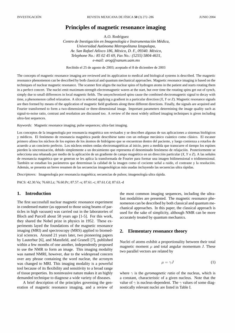
Beff =B1and the precession of M takes place around the vec-tor B1. We are referring to precession as seen in the rotatingframe of reference in which B1 is static as indicated in Fig. 3.If we apply the oscillating magnetic field for a short period,t1with amplitude B1, the magnetization will precess throughan angle θ=γB1t1. If θ=π, then the pulse inverts the magneti-zation. This pulse is called a 180 pulse. And, if θ=π/2 (90

pulse), then the magnetization is rotated from the Z-directionto the -Y-direction. After a 90 pulse the magnetization pre-cesses in the laboratory frame, pointing normal to the staticfield. The pulses described here are usually referred to as RFpulses.

FIGURE 2. The Larmor precession of a magnetic moment in a uni-form magnetic field.

Rev. Mex. Fıs. 50 (3) (2004) 272–286

PRINCIPLES OF MAGNETIC RESONANCE IMAGING 275

FIGURE 3. a) Effective field Beff in the rotating frame. b) Themagnetisation about Beff .

4. The Bloch equations and relaxation times

So far, we have not taken into account the interactions be-tween the spins and their environment, since we were deal-ing with isolated spins. However, for a sample made up ofmatter, it is necessary to consider the internal magnetic andelectric fields. These fields can cause additional motion of themagnetization, known as relaxation. The problem of the evo-lution of the magnetization under the influence of the sum ofa constant, and a rotating field with simultaneous relaxationwas first solved by Bloch [3]. He proposed a set of equationswhich describe how a spin system evolves. Thus,

dMz

dt=

M0 − Mx

T1+ γ (M × B)z (23)

dMx

dt= γ (M × B)x − Mx

T2(24)

dMy

dt= γ (M × B)y − My

T2(25)

where B=B+B1. Two different times T1 and T2 have beenintroduced, which are the longitudinal relaxation time and the

TABLE II. Representative values of approximate relaxation timesfor hydrogen components of different human tissues at 1.5 Teslaand 37C.

Tissue T1 (ms) T2 (ms)

gray matter 950 100

white matter 600 80

muscle 900 50

cerebrospinal fluid (CSF) 4500 2200

fat 250 60

blood 1200 100-200

transverse relaxation time respectively. The transverse rate ofdecay may differ from the longitudinal one.

In terms of the original variables, the complete set of so-lutions is therefore

Mx(t) = exp(−t

T2

)(Mx(0) cos(ω0t)

+My(0) sin(ω0t)) (26)

My(t) = exp(−t

T2

)(My(0) cos(ω0t)

−Mx(0) sin(ω0t)) (27)

Mz=Mz(0) exp(−t

T1

)+Mz(0)

(1− exp

(−t

T1

))(28)

Spin-lattice relaxation, which is characterized by T1, thespin-lattice relaxation time occurs as a result of an exchangeof energy between the spin system and the lattice. The lat-tice is defined as the assembly of sample molecules treatedas a reservoir of thermal energy, determined by the motion ofmolecules. The transverse magnetization is not related to theenergy of the spins and its evolution is influenced by quantumtransitions, which cause the transfer of energy between spins,leaving the total energy unchanged. This process is calledspin-spin relaxation and is defined by T2, the spin-spin relax-ation time.

Inhomogeneity in B also gives rise to decay of trans-verse magnetization characterized by a decay time, T2*. Inthis case, the precession vector proceeds at different rates indifferent sections of the sample. This accelerates the processof transverse relaxation, so that T∗

2 <T2.In the rotating frame, Bloch’s equations can be solved for

continuous irradiation with a weak RF field, so that, satu-ration is avoided. This saturation condition means that thedecay of the transverse magnetization resulting from a π/2 iscomplete before another pulse is applied. In other words,after a π/2 pulse there is no magnetization along the Z-direction: a new π/2 pulse transmitted at the time would re-sult in no FID signal, as there would be no longitudinal mag-netization to rotate into the transverse plane. In this case, themagnetization precesses around Beff (see Fig. 3). Neglect-ing the transient term, substituting M=χB, and defining

Rev. Mex. Fıs. 50 (3) (2004) 272–286

276 A.O. RODRIGUEZ

ω=γ B, then the steady state solutions can be expressed asMx=χ′H1and My=χ′′H1

Dispersion mode.

χ′ =χ0

2T2ω0

(ω0 − ω)T2

1 + (ω0 − ω)2T2(29)

Absorption mode.

χ′′ =χ0

2T2ω0

11 + (ω0 − ω)2T2

(30)

χ = χ′ − iχ′′ (31)

χ is the complex susceptibility and χ is the sample’s staticsusceptibility. Eqs. (30) and (31) describe the NMR line-shapes predicted by Bloch’s equations as shown in Fig. 4.

5. Free induction decay and spin echoes

If a specimen is left in a high magnetic field for a long enoughtime, protons in the sample will tend to align themselvesalong the direction of the external magnetic field. Forminga macroscopic nuclear magnetization of the sample. But, ifthe magnetization is perturbed away from alignment with thefield, using a 90 pulse, precession of the resulting magne-tization will occur. There will be a gradual dephasing ofthis magnetization and consequently a loss of coherence ofthe precessing magnetization. The dephasing of the trans-verse magnetization causes a gradual decrease of the signalinduced in the RF coil, leading to a decaying NMR signalwhich is called the free induction decay (FID). (That is, de-cay free of B1). This represents the total time-varying coher-ent magnetic field derived from the sum over all precessingproton spin fields, which induce a small EMF in any RF coilproperly oriented to detect the corresponding flux changes. Itcan be used to locate the resonance peak for water, and de-termine the RF amplitude and duration necessary to producemaximum signal. The theoretical expression for the FID forthe complex form of a demodulated signal due to an RF spinflip at t=0 is:

s(t) ∼ ω0

∫d3re(− t

T2(−→r )) |B| (−→r ) |M(−→r , 0)|

×ei(t(Ω−ω(−→r ))+φ0(−→r )−θB(−→r ) (32)

FIGURE 4. Lorentzian lines for absorption and dispersion.

where φ0is the magnetization phase (the phase angle givesthe direction in the X-Y plane of the two-dimensional trans-verse magnetization vector), Ω is the demodulation referencefrequency, and field angle θB . In 1950, Hahn [8] showedthat an echo of the MR signal could be forced by subjectingthe sample to two RF pulses. Hahn applied a π/2 pulse (90

pulse) to a sample to observe a FID which follows a turn-offof the pulse. Inhomogeneities cause a spread in the preces-sion frequency, so that some of the spins go out of phase withrespect to the others. Because of this dephasing, the resultantsignal decays with a time of the order of 1/(γ∆B), where ∆Bis the spread in the static field over the specimen. If how-ever a second π/2 pulse is applied at a time τ after the firstpulse, another signal re-appears at a time 2τ after the initialpulse. He named the signal the spin echo. Later, Hahn him-self showed the existence of echoes from Bloch’s equations.This solution proved that if τ is varied the echo amplitude di-minishes exponentially with a time constant T2. A pictorialdescription of the process of echo formation in a 90-τ -90

sequence is shown in Fig. 5.

6. Fourier transform NMR

The early NMR experiments used continuous wave (CW) de-tection. Nowadays, systems use the so called Fourier Trans-formation NMR methods, which employ short intense RFpulses, to excite a wide bandwidth of frequencies simulta-neously. Recently the wavelet transform has also been usedto generate an image from MR signals [9]. The Fourier trans-form of the resulting FID reveals the mixture of frequenciesproduced by the applied gradients, chemical shift variations,etc., for on resonance spin species. The FID is the expo-nential T2 decay whose Fourier transform is the lineshape ofEq. (30). Experimentally, the lineshape will be broader thanthat predicted by T2 relaxation only. This is because the

FIGURE 5. The Hahn spin experiment: i) application of π/2 pulse,ii) dephasing of spins, iii) position of spin isochromats following aπ pulse, and iv) position of magnetisation after refocusing.

Rev. Mex. Fıs. 50 (3) (2004) 272–286

PRINCIPLES OF MAGNETIC RESONANCE IMAGING 277

magnetization is also attenuated by dephasing magnetic fieldinhomogeneities. This is added to the decay function to yieldthe effective decay time, where

1T ∗

2

=1T2

+1

T2in(33)

T2in is the effective relaxation time due only to inho-mogeneities. To excite all the spin frequencies of interestthe RF pulse should have a bandwidth large enough to spanthe appropriate frequency range. The bandwidth can be cal-culated from the Fourier transformation of the pulse shape.The linewidth of the resonance peak can be obtained FromEq. (30). Defining the linewidth ∆f as the width at halfheight, then

∆f =1

πT2(34)

The Fourier transformation of a single FID can produceall the necessary information to create a spectrum.

7. The chemical shift

Other important NMR parameters that can distinguish spins ina particular environment are: the self-diffusion coefficient D,the isotropic chemical shift δ, and the hyperfine splitting J.In a real spin system, all nuclei in atoms and molecules haveassociated electrons. If a magnetic field is applied, the sur-rounding electron clouds tend to circulate in such a directionas to produce a field which opposes that applied, causing asmall chemical shift. The nucleus experiences a total field:

Beff = B0(1 − d) (35)

where d is the shielding. This shielding perturbation resultsin a shift of the resonant frequency for nuclei in different en-vironments, and this resultant effect is very useful in NMRspectroscopy. The chemical shift may be expressed as,

δ =f − fTMS

fTMS106 (36)

where δ is in parts per million (p.p.m.), f is the resonantfrequency of the species of interest, and fTMS is the reso-nant frequency of a reference substance (TMS: tetramethyl-silane). The effect of chemical shift is observed in imageswhere more than one chemical is present. The value of δ isvery small, usually on the order of a few parts per million andis dependent on the local chemical environmental in whichthe nucleus is situated. Fat (CH2) is a well-known exampleof a chemically-dependent component which is chemicallyshifted about a 3.35 ppm in Larmor frequency from water(H20) protons. A large range of δ values exist for biologicalobjects giving rise to many resonant frequencies. It is validto assume that the resonant frequency range of a spin systemcan be expresses as

|ω − ω0| ωmax

2(37)

8. Image formation

To form an image is necessary to perform the spatial localiza-tion of the MR signals which is normally a two step process.First a slice of the body is selected for imaging. Second amagnetic field gradient can be applied along to any or a com-binations of following directions X, Y, and Z, and accordingto a preestablished imaging sequence to generate an imagewith a specific orientation.

8.1. Magnetic field gradients

In order to generate an image, it is necessary to measure thespatial variation of MR parameters such as spin density, or thespin-lattice relaxation time, T1. These variables are not inde-pendent of the spatial coordinates of the spin system. Thesemeasurements are made by degrading the uniformity of thestatic magnetic field so that the magnetization precesses atdifferent frequencies. Therefore, there is a variation of res-onance frequency across the sample. We may modify theuniformity of the field B by applying linear magnetic fieldgradients across the sample. The Hamiltonian describes theinteraction of isolated spins at position r in a magnetic fieldgradient as follows

H =h

2π(ω0Iz + γI · G · r) (38)

where G is a magnetic field gradient tensor containing ninecomponents. The only terms which contribute significantlyare the Z-axis ones. Therefore, the effective gradient Hamil-tonian is

H1 = γ∑

i

(G · ri)Izi (39)

where G has the components

Gx =∂Bz

∂x(40)

Gy =∂Bz

∂x(41)

Gz =∂Bz

∂z(42)

To generate a one dimensional image we simply acquirethe NMR signal in the presence of a spatially varying mag-netic field which is added to the uniform field [6-7]. If alinear gradient in the Z-direction is employed, the resultingmagnetic field parallel to the uniform field is

Bz = B0 + z∂Bz

∂x(43)

Therefore, the variation of the resonance frequency withposition can be expressed

ω0(z) = γBz = γ(B0 + Gzz) (44)

Rev. Mex. Fıs. 50 (3) (2004) 272–286

278 A.O. RODRIGUEZ

From Eq. (44) we can appreciate that the gradient givesa linear variation of frequency with position. The mag-netic field now has varying amplitude for spins along theX-direction. For a one dimensional object, the FID is thesum of all the individual contributions from spins at differ-ent positions. The decomposition of the FID into a frequencyspectrum is obtained using the Fourier transformation of theMR signal. The effect of a linear gradient applied across atwo-dimensional sample is shown in Fig. 6.

8.2. Selective excitation

When applying common NMR techniques, the excitationspectra of the applied RF pulses (non-selective or hard pulse)are many times broader than the spin absorption spectrum, sothat the whole sample is excited by the RF pulse. In MRI,

FIGURE 6. a) Application of a linear gradient field to a sample, b)projection of the sample spin distribution, and c) selective excita-tion of a plane of spins in a cylindrical sample.

however, we are usually interested in exciting a thin sliceof the sample. This can be done by simultaneously apply-ing a magnetic field gradient and a selective pulse [10]. Asuitable shaped selective RF pulse (amplitude modulation intime) is required to excite only a limited section of the fre-quency spectrum. In the presence of a magnetic field gradientsuch a pulse will only excite a slice of the sample. The thick-ness of the slice is proportional to the spectrum width. Thiseffect can be seen from the spatial variation of the transversemagnetization after application of a rectangular pulse of du-ration th in the presence of a Z-gradient, Gz . The magnitudeof the transverse magnetization is [10]

[M2x + M2

y ]1/2 = m sin(θ)[cos2(θ)

×(1 − cos2(γBeff th))2 + sin(γBeff th)2]1/2 (45)

and its phase is defined by

φ=tan−1

[Mx

My

]= tan−1

[cos(θ)(1− cos(γBeff th))

sin(γBeff th)

](46)

where Beff is the effective field, and θ is the angle Beff

makes with Z-axis which are given by

Beff =[B2

1 + Gz(z − z0)2]1/2

(47)

θ = tan−1

[B1

Gz(z − z0)

](48)

For small values of B1 such that

B1

Gz(z − z)0 1 (49)

this reduces to

| M | =2B1M0

Gz(z − z0)sin

[γGz(z − z0)th

2

](50)

θ =γGz(z − z0)th

2(51)

Thus the shape of the slice (sinc) corresponds to theFourier transform of the applied pulse (top hat), and the widthof the selected slice is inversely proportional to Gz. The phasevariation with Z means that there will be little total transversemagnetization at the end of the pulse application. The phasevariation can, however, be eliminated by applying a gradi-ent, Gz of opposite polarity for a time, th/2. For generalpulse shapes the form of the excited slice follows the pulsespectrum only for low angles, and more powerful techniquesmust be used to design pulses to excite rectangular slices withlarge flip angles. The relation between the slice select gradi-ent used and the orientation of the slice plane produced issummarized in Table III.

TABLE III. Image orientation and the gradient coils used.

Applied slice select gradient name slice plane orientation

Gx sagittal parallel to y-z plane

Gy coronal parallel to x-z plane

Gz transverse parallel to x-y plane

Rev. Mex. Fıs. 50 (3) (2004) 272–286

PRINCIPLES OF MAGNETIC RESONANCE IMAGING 279

Multi-dimensional RF pulses can also be applied in awide variety of MR applications in which transverse mag-netization is to be excited, or to be refocused within a well-defined spectral or/and spatial region.

8.3. The k-space concept

This is a very important concept in MRI since it allows us tomanipulate how the data are acquired, manipulated, and re-constructed for viewing. The k-space can be simply definedas the abstract platform onto which data are acquired, posi-tioned, and then transformed into the desired image. There isno such agent in any other imaging modality (x ray-imaging,Positron Emission Tomography, Computerised Tomography,Ultrasound). The choice of the letter k is based on the tradi-tion among physicists and mathematicians to use that letterto stand for spatial frequency in other similar equations, andhas no particular significance at all.

The MR signal as a function of time produced by the slice,omitting relaxation effects [10], is given by

S(t) =∫

ρ(r) exp(iγ

t∫0

r · G(t′)dt′)dr (52)

where ρ(r) is the spin density at position r. Mansfield andGrannell [7] realized that there is a similarity between theMRI signal and the Fraunhofer diffraction pattern of scatter-ing plane waves. A diffraction pattern is generated and itsFourier transform is the image of the object. In our situation,the plane wave is more of a theoretical concept rather thana real wave, but it can help in the study and design of pulsesequences. Mansfield and Grannell introduced the concept ofthe reciprocal space wave vector

k = γ

t∫0

r · G(t′)dt′ (53)

where k is a vector in k-space. From Eq. (52) and Eq. (53)the signal can be written as:

S(k) =∫

ρ(r) exp(ik · r)dr (54)

It is not very difficult to see that the parameter k describesa trajectory scanning through k-space as the time t of Eq. (54)changes. k-space contains all the information required toform an image and allows us to depict graphically most ofthe MRI techniques. Some k-space trajectories of commonimaging techniques are shown in Fig. 7. The spatial res-olution achievable in MRI is established by the wavelengthλ = 2π |k| − 1. This parameter indicates that spatial reso-lution does not depend on the wavelength of the RF at theoperating frequency. The resolution of an image in the X-direction, can be measured as a function of the maximumspatial frequency kmax sampled in the experiment:

∆x =π

kmax(55)

FIGURE 7. k-space trajectories corresponding to well-knownimaging schemes: a) Projection Reconstruction (PR), b) Two-Dimensional Fourier Transform (2D-FT), c) Echo-Planar Imaging(EPI). d) The Modulus Blipped Echo-Planar Imaging (MBEST). e)Spiral Echo-Planar Imaging (SEPI), e) Square Spiral Echo-PlanarImaging (SSEPI).

For a time independent gradient G, which is applied for atime td, kmax can be written as:

kmax = γGtd (56)

Hence, from Eq. (56) the image resolution can be increasedby augmenting the gradient amplitude or the time duration,to sample higher spatial frequencies.

9. Magnetic resonance scanner

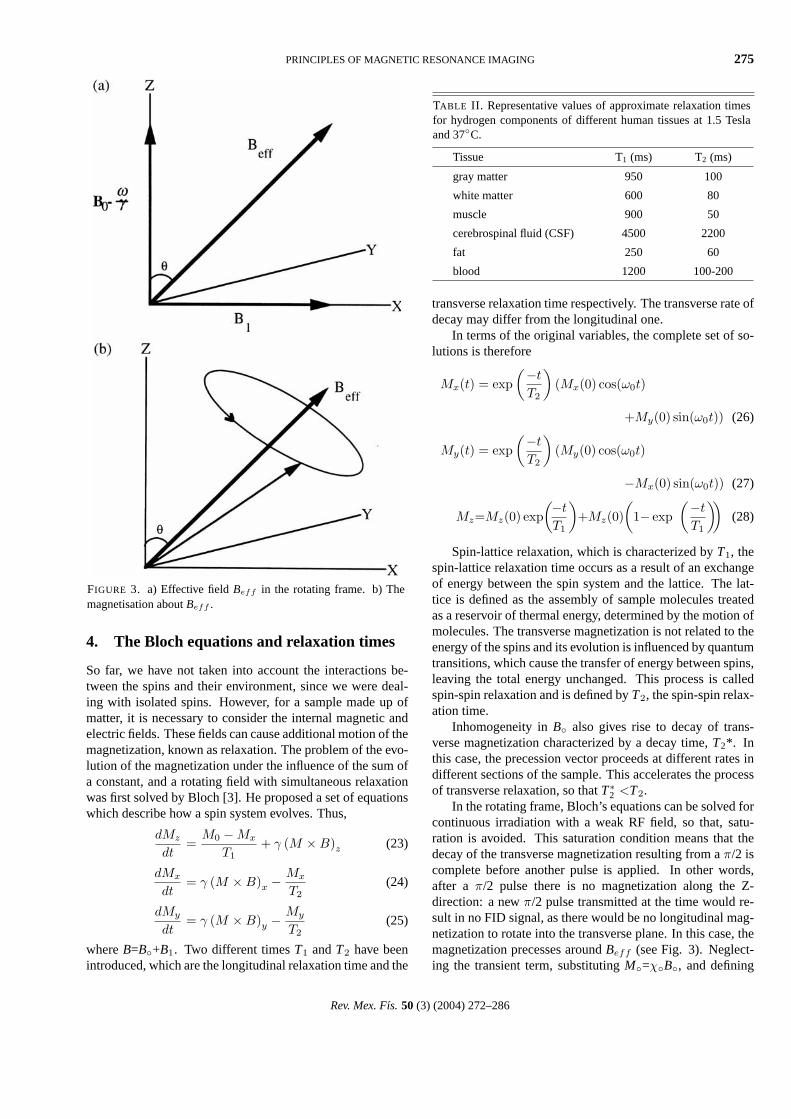
A number of processes must be completed to produce MRimages. These processes include nuclear alignment, RF ex-citation, spatial encoding, and image formation. In simpleterms, an MRI system consists of five major components:a) a magnet, b) gradient systems c) an RF coil system, d) areceiver, and e) a computer system. Fig. 8 shows a blockdigram of the main components of MR scanner for clinicalapplications. All of which must be taken into account whendesigning a suitable site and all of which have their own spe-cial problems.

Rev. Mex. Fıs. 50 (3) (2004) 272–286

280 A.O. RODRIGUEZ

FIGURE 8. Diagram of whole-body magnetic resonance imager.

a) Magnet. The magnet aligns the nuclei into low energy(parallel) and high energy (anti parallel) states. There-fore, a strong magnet is necessary to generate a highmagnetic field (B0), which should be uniform over avolume of interest. A high-field magnet provides betterSNR resolution both in frequency and spatial domains.However, the main requirement for the B0 field, is thatits field uniformity should be very good. A few partsper million over a spherical volume, 50 cm in diame-ter, are required for a great variety of clinical applica-tions. The optimal field strength and the type of magnetfor imaging are dependent on the application so per-manent, resistive, or superconducting magnets may beused. For most clinical MRI systems Bvaries from0.05 to 3.0 Tesla, and permanent and superconductingmagnets are mainly used. Superconducting magnetsare made of a niobium-titanium alloy and are cooledto temperatures below 12 K by immersion in liquid he-lium, whose boiling point is 4.2 K. The main magnetrarely produces a field of sufficient uniformity by itself,so to maintain the magnetic field homogeneity a shimsystem is necessary.

b) Gradient coils. All type of MRI modalities requireto deliberately alter the field uniformity by applyinga magnetic field gradient Gz(r), which varies lin-early with position r to spatially encode the NMR sig-nal. Such gradients are generated by passing currentsthrough specially arranged coils of wire, placed on a

former that surrounds the imaging subject. Three sep-arate coils are needed in order to produce a linear vari-ation of the Z-component of the magnetic field alongeach of the three Cartesian directions (see Table III).Many clinical MR systems are capable of producing40 mT m−1 gradients to this end.

c) RF coil system. In MRI is necessesary to irradiate thesample under test with an RF field (B1), in order toflip the magnetization away from its equilibrium stateand generate a detectable NMR signal. This is usu-ally done with an RF transmitter which is responsiblefor pulse shape, duration, power, and timing (repeti-tion rate). Since the imaging subject is excited withan RF field, each spin produces a sinusoidal signal ata frequency dependent on the local magnetic field. Todetect the signal coming from the spins is necessary adevice to couple the nuclei to some external circuitry.These devices are called RF coils, or RF resonators,or RF probes. RF coils can be divided in two maingroups: volume and surface coils. Volume coils aretypically cylindrical-shaped structures, and the mostefficient volume coil to the present time is the so calledbird-cage coil. Surface coils can be subdivided intosingle-loop coils and array coils (phased- array coilsand array of independent coils for ultra-fast imagingschemes).

d) Receiver system. To convert the received RF signalfrom the RF coil into form suitable for an analog-to-digital converter (ADC) or digitizer, some receiver cir-cuitry is often employed. The signal is first amplifiedwith a low noise amplifier, then is transmitted to a re-mote location to form an image via a computer pro-cessing. The rest of the process involves signal de-modulation using a superheterodyne style circuit. Thisis normally done with respect to the same frequency asthe emitted RF radiation.

e) Computer system. This system represents the inter-face through which the user initiates measuring sys-tem functions (system test, display images, measurefunctions) and usually retrieves images. In particular,for the reconstruction process, the computing require-ments varies according to the imaging method used,but almost universally some form of Fourier transform(FT) is required. The best algorithm for FT is the fastFourier transform (FFT), which can be used for two-or three-dimensional images. The computer systemshould also be able to display images on a high-qualitymonitor.

10. Overview of MRI methods and techniques

The imaging methods will be divided into four categories:point, line, planar (two dimensions), and three dimensionalimaging, depending on the manner in which the image data

Rev. Mex. Fıs. 50 (3) (2004) 272–286

PRINCIPLES OF MAGNETIC RESONANCE IMAGING 281

points are acquired. This is to say, it is usually by the sim-ple expedient of replacing one stage of the imaging processby a selective excitation. It is clear from their ability to re-ceive the signal, simultaneously from the entire region of in-terest, that planar and three dimensional techniques will bemore efficient than point and line methods, in terms of imagesignal-to-noise ratio (SNR) per unit time, and will thereforebe preferred in most situations.

10.1. Point and line methods

The point methods have the advantage of being very simpleexperimental methods. Usually they do not require a greatdeal of hardware and the field homogeneity only has to begood over a very small region. One example of these pointmethods is the so called FONAR (Field Focused NuclearMagnetic Resonance) method, introduced by Damadian [11].It is well known, that the FID obtained from a sample lo-cated in an inhomogeneous magnetic field will decay rapidly.This occurs because different regions of the sample are lo-cated in different magnetic fields. And, the signal thereforehas a wide range of frequency components which rapidly de-phase giving a shortened FID, and correspondingly a broadlineshape on Fourier transformation. A sample which is suf-ficiently large to extend beyond the homogeneous region of amagnet will therefore give rise to a signal (to a first approxi-mation) with two components: one which is long-lived fromthe central homogeneous region, and one which is short-livedfrom the surrounding non-homogeneous region. A selectivepulse with an adequately narrow bandwidth can be used toexcite only those spins inside the resonance aperture (signal-producing region). An image can then be produced point bypoint, by moving the sample relative to the magnet or by re-locating the resonance aperture.

Hinshaw [12] introduced another point method whichemploys three sinusoidal oscillating orthogonal field gradi-ents, which define a small region at their intersection. Onlythe spins within this region are in a time-invariant magneticfield. This region called the sensitive point, generates a signalwhich is acquired using a narrow band filter. This is a straightforward technique to implement since there is no need forcomplicated image reconstruction and little dependence ongradient linearity. This method allows localised NMR mea-surements to be made without the necessity of forming an im-age, so it could be used to measure T1. But, the long imagingtime is its major disadvantage. These methods are an exten-sion of the point methods. The basic idea is to isolate a linewithin a three dimensional object and subsequently to distin-guish between signal emanating from different points alongthe selected line. These methods are insensitive to magneticfield inhomogeneities though to a lesser degree than the pointtechniques.

10.2. Two-dimensional techniques

Most MRI experiments are sequential plane techniques in thesense that a slice of magnetization is excited prior to data

acquisition. This is done by using some form of selective ir-radiation as described previously. Imaging sequences may bedivided into two groups: a) frequency encoding of the spinsystem, and b) phase encoding. We shall start with the sim-plest technique which uses frequency encoding.

10.2.1. Backprojection reconstruction

This method is normally used in X-ray CT, and was intro-duced into MRI by Lauterbur [6]. The signal obtained froma sample in the presence of an applied gradient correspondsto a one-dimensional projection of the object onto the axis ofthe gradient. An image can be constructed by altering the di-rection of this gradient to collect a number of projections ofthe object, and then processing these profiles using a recon-struction algorithm. The total spin density contributing to afrequency ∆ω = γGφr, to each ray (r,φ), is given by the lineintegral:

P (r, φ) =∫

Γ,φ

ρ(x, y)ds (57)

where s is the distance along the ray direction. Each value ofP(r,φ) is called a ray sum, and the set of values for a givengradient orientation φ as the projection at angle φ. Eq. (57)represents a NMR spectrum, which is the Fourier transformof the FID obtained from the gradient Gφ. A set of projec-tions P(r,φ) is acquired by rotating the gradient angle. Theseare then filtered, and back projected to form an image.

10.2.2. Fourier imaging

The Fourier method was first developed by Kumar and et. al,in 1975 [13], and can be considered to be a typical two di-mensional spectroscopy technique. The most popular classof planar methods are currently the two dimensional Fouriertechniques, for short 2D-FT. The basic idea is to apply a 90

RF pulse, and a slice selection gradient to generate an FIDwhich evolves first under the influence of a field gradient, Gy

for a time ty , followed by a second gradient, Gx with dura-tion t, which is applied at a right angles to the first. The signalis phase encoded during the application of the first gradient,and sampled for times tx during the spatial encoding, readgradient, Gx. Excluding relaxation effects, the signal is:

S(tx, ty)=∫∫

ρ(x, y) exp [iγ(Gxxtx+Gyyty)] dxdy (58)

The experiment is then repeated with an incrementingperiod of evolution under the gradient Gy . In these experi-ments, k-space is filled with one line at a time. After the fulldata acquisition is done, a two dimensional Fourier transform(2D-FT) yields the spin density distribution. The sequence ofRF pulses and gradient pulses is shown in Fig. 9. Edelsteinand et al. [14] modified the Fourier imaging method, to in-troduce another method called spin-warp imaging, in which aphase variation is generated by changing the gradient ampli-tude with the phase encoding carried out for a constant timeperiod. This has the advantage that effects remain constant

Rev. Mex. Fıs. 50 (3) (2004) 272–286

282 A.O. RODRIGUEZ

FIGURE 9. The sequence of RF pulses and gradient pulses for 2D-Fourier Transform Imaging.

throughout the experiments. A timing diagram for the 2D-FTspin-warp imaging sequence is shown in Fig. 10.

10.3. Full and half Fourier imaging

Whenever the four k-space quadrants are scanned, filling thewhole of the space, this is designated as a Full Fourier tech-nique. The Fourier transform generates information con-taining real and imaginary parts with a well defined phase.Taking the modulus of the two parts, gives rise to modulusimages in which all phase effects are removed. However,these methods can require long imaging times. To abbreviatethe long imaging times of the Full Fourier methods, we canscan only half of the k-space [15-16], and then reconstructthe other half using the Hermitian symmetry property of theFourier transform of the MR signal, S(-k) = S*(k) [15]. Then,in some cases only half the number of the experiments arerequired. This method requires zero filling of the data beforeFourier transformation. Filtering is needed to avoid ringingat the edges produced by the truncating step function. Phasevariation causes problems since the Hermitian symmetry islost. Such phase variation results from field inhomogeneity,misalignment of the signal detection, and gradient eddy cur-

FIGURE 10. A timing diagram for the 2D-FT Spin Warp scheme.

rents. These problems can be overcome by using anothertype of partial sampling scheme, which makes use of slightlymore than half of the k-space data in one encoding direc-tion [17-18]. This enables us to construct a coarse phasemap from the symmetric data around the origin, which willbe employed afterwards to correct the phase errors, seeFig. 11(e). Some Half Fourier sampling strategies are illus-trated in Fig. 11.

10.4. Three-dimensional techniques

It is possible to extend the two dimensional techniques to pro-duce three dimensional imaging. Three-dimensional data setscan be generated in many different ways from Fourier tech-niques, for example, by multislice imaging or by using ad-ditional phase encoding. The multislice technique can pro-duce images of different sections. The slice of the objectgoes through a cycle during the interval TR, during this timea different slice is selected and then imaged. Most of theimaging time is spent in waiting for T1 recovery of magneti-zation (TR). A 3D FT image can be acquired by repeating a2D-FT process a certain number of times without slice selec-tion, where the repetition number depends on the number ofslices thatarerequired.Theinformationinthe Z-axisisencoded

Rev. Mex. Fıs. 50 (3) (2004) 272–286

PRINCIPLES OF MAGNETIC RESONANCE IMAGING 283

FIGURE 11. k-space can be scanned in different ways: a) symmet-rically about the centre, b) alternate phase-encoding lines, c) non-positive phase-encoding steps, d) in the readout direction, and e)partial scanning in the readout direction. The horizontal directionis the readout time. The shaded areas correspond to the experimen-tally acquired data and the other lines are zero.

in the same way as it is encoded along the Y-axis by the useof an additional phase encoding gradient. The Fourier trans-form is applied successively three times to reconstruct the 3Dimage.

10.5. Chemical shift imaging

MRI and MRS have been developed somewhat indepen-dently, and the information provided by these two techniquesis complimentary. MRI exclusively uses the proton (1H) res-onance, to yield spatially-resolved images with no discrimi-nation among signals arising from hydrogen nuclei existingin different chemical groups (no chemical shift resolution).MRS is able to yield NMR spectra in which chemical shiftresolution is very important. Such spectra contains no spa-tial information. Thus it has long been desired to obtainboth spectrally and spatially-resolved information in a sin-gle study. These two sources of biological information canbe put together in the so called chemical shift imaging orspectroscopic imaging. This imaging technique is referredto the process of selectively imaging (or obtaining the spa-

tial distribution) of identical nuclei that different levels ofmagnetic shielding due to their chemical environments asshown in Eqs. (35) & (36). The possibility of observing bodychemistry at the same time as producing an image is a bonuswhich, if applied clinically, could uniquely pinpoint regionalmetabolic disorders in tissues and organs.Via chemical shiftimaging, the clinician and the researcher are able to gleaninformation of a truly chemical and biochemical nature in acompletely non-invasive manner.

11. Contrast and signal-to-noise ratio (SNR)

An important aim of imaging for diagnostic purposes is to beable to distinguish between diseased and neighbouring nor-mal tissue. MRI offers important advantages when comparedwith other imaging modalities due to its excellent soft tis-sue discrimination of the images. MRI has an abundance ofsignal-manipulating mechanisms, as the signal is dependentof a wide variety of tissue parameters. A contrast in the im-age can then be created to meet certain demands. Image con-trast is defined in terms of differences in image intensity asfollows:

CAB =|ImA − ImB |

Imref(59)

where ImA and ImB are the image intensity of tissues Aand B, and Imref is a normalising value. Im is a function ofspin density σ, T1, T2,T∗

2 and diffusion coefficients D. If thedata acquisition parameters are chosen such that the T1 effectis dominant, then

CAB ≈ f(T1) (60)

and the resulting images is said to carry T1 contrast or a T1

weighting. Similarly for T2 contrast and spin density con-trast:

CAB ≈ f(T2) (61)

and

CAB ≈ f(σ) (62)

Spin density contrast is linearly proportional to the tis-sue spin density difference, whereas T1, T2 contrasts havean exponential dependence on the tissue T1, T2 values. Nor-mal soft tissue usually have a small variation in spin density,but have quite different T1 values. Therefore, T1-weightedimaging is an effective method to obtain images of a goodanatomical definition. Many disease states are characterizedby a change of the tissue T2 value, and T2-weighted imagingis a sensitive method for a disease detection. Fig. 12 showsT1 -weighted and T2-weighted images of brain obtained at1.5 Tesla.

Rev. Mex. Fıs. 50 (3) (2004) 272–286

284 A.O. RODRIGUEZ

FIGURE 12. A T2-wheighted image (left) and T1-weighted image(right) of the human brain.

In any physical measurement there is always presentnoise either random or systematic which diminish the imagequality. Random noise often arises in an imaging system be-cause of spontaneous fluctuations such as the thermal noise(Brownian motion) of free electrons inside real o equivalentelectrical components. This noise is sometimes called John-son noise. The degree to which noise affects a measurementis generally characterized by the SNR. This is the ratio of theamplitude of the signal received to the average amplitude ofthe noise. The signal is the voltage induced in the receivercoil by the precession of the magnetization in the transverseplane. The noise is generated by the presence of the patientin the magnet, and the background electrical noise of the sys-tem (coil and electronics). It is also known that the varianceof the fluctuating noise voltage is

σthermal =√

4κTR BW (63)

where R is the effective resistance of the coil loaded by thebody, and BW is the bandwidth of the noise-voltage detectingsystem. Both the signal and noise are detected by the receivecoil, and the bandwidth is determined by the cutoff frequencyof the analog low pass filter. The SNR can be defined as,

SNR =signal

resistance=

S(k)Reff

(64)

SNR =∫

ρ(r) exp(ik · r)dr

Rbody + Rcoil + Relectronics(65)

From Eq. (65) can be appreciated that to increase theSNR can be done by a) reducing the effective resistance: thiscan be achieved by reducing the coil and electronics resis-tance, this demands better coil designs with low resistancevalues, b) increasing the MR signal with high-field MR scan-ners. High field MRI promises to improve anatomic imag-ing quality by factors, and to bring metabolic and functionalimaging to the forefront of diagnostics modalities. There aresystems available with field strengths up to 22 Tesla, but forclinical purposes the highest field is 3 Tesla. Although it ispossible to purchase whole-body systems of 7 T or 8 T forMRI applications in humans. The SNR is also an importantparameter to measure performance of a MR imager.

The size of the spatial features that can be distinguishedin a MR image can be defined as the resolution, and does notdepend on the wavelengths of the input RF field.

12. Ultra-fast imaging

The development of faster magnetic resonance imaging hasmainly been motivated by the long acquisition times com-pared to physiological motion and patient tolerance. Theselong times cause imaging artefacts, a limited number of appli-cations and increased costs. Respiration, pulsation peristalsisoccur during the exam can result in substantial distortion ofthe image. Artefacts from patient motion can drastically de-grade the image quality, due to discomfort originated by ex-ams with long duration times. This exacerbated in patientswith pain and suffering from claustrophobia. Shorted scan-ning times can reduce the cost of a conventional MRI exam.

MRI offers alternatives to reduced-time acquisitionschemes. In the most commonly used imaging sequence,multislice two-dimensional Fourier transform (2D-FT), thescan time Tscan is given by the following simple relationship:

Tscan = NY TR NEX (66)

where N is the number of phase-encoding samples, TR thepulse repetition time, and NEX the number of excitations(also termed number of acquisitions or number of averages)used for signal averaging.

12.1. Fast Fourier imaging

The spin-warp imaging technique owes its popularity in theclinical environment to its robustness, however in its simplestform it requires long imaging times. In an effort to reducescan time, Haase and co-workers [19] introduced an imag-ing method called Fast Low Angle Shot: FLASH. This isbasically the gradient echo version of the 2D-FT techniquewith a very short repetition time TR. Reduction of the echotime necessitates the use of a low angle RF pulse for slice se-lection, typically around 15, for maximum SNR. There areother techniques which are based on the same principles, suchas the Snapshot/Turbo FLASH and Gradient Recalled Acqui-sition in the Steady State (GRASS) techniques [20]. GRASSis a very similar technique to FLASH, which only differs inthat an additional phase encoding gradient is applied after thesampling period. This gradient has an opposite sign to thefirst one, so it can rephase any transverse magnetization re-maining at the end of the experiment. Consequently, the SNRis improved and image artefacts are removed.

12.2. Echo-planar imaging

Echo Planar Imaging (EPI) was introduced by Mansfieldin 1977 [21], and is a true snapshot technique which enablesthe formation of a complete image in 30-100 ms. The rapidnature of this technique is due to the fact that only one RF

Rev. Mex. Fıs. 50 (3) (2004) 272–286

PRINCIPLES OF MAGNETIC RESONANCE IMAGING 285

excitation is needed per image. It thus allows the acquisi-tion of a two-dimensional image from only one FID. Fol-lowing the excitation of a slice, the signal is sampled underthe influence of two orthogonal gradients. A gradient Gx

(X-axis) is modulated rapidly to generate a series of gradi-ent echoes. This forms the frequency encoding part of theexperiment. In conjunction with Gx, another gradient Gy

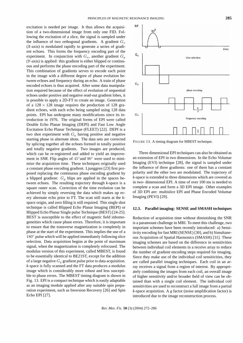
(Y-axis) is applied: this gradient is either blipped or continu-ous and performs the phase encoding part of the experiment.This combination of gradients serves to encode each pointin the image with a different degree of phase evolution be-tween echoes and frequency during an echo. A train of phaseencoded echoes is thus acquired. After some data manipula-tion required because of the effect of evolution of sequentialechoes under positive and negative read-out gradient lobes, itis possible to apply a 2D-FT to create an image. Generationof a 128 × 128 image requires the production of 128 gra-dient echoes, with each echo being sampled using 128 datapoints. EPI has undergone many modifications since its in-troduction in 1976. The original forms of EPI were calledDouble Echo Planar Imaging (DEPI) and Fast Low AngleExcitation Echo Planar Technique (FLEET) [22]. DEPI is atwo shot experiment with Gy having positive and negativestarting phase in alternate shots. The data sets are correctedby splicing together all the echoes formed in totally positiveand totally negative gradients. Two images are produced,which can be re-registered and added to yield an improve-ment in SNR. Flip angles of 45and 90 were used to mini-mize the acquisition time. These techniques originally useda constant phase encoding gradient. Ljunggren [23] first pro-posed replacing the continuous phase encoding gradient bya blipped gradient: Gy blips are applied in the spaces be-tween echoes. The resulting trajectory through k-space is asquare raster scan. Correction of the time evolution can beachieved by simply reversing the data which makes up ev-ery alternate echo prior to FT. The scan still starts at the k-space origin, and zero filling is still required. This single shottechnique is called Blipped Echo Planar Imaging (BEPI) orBlipped Echo Planar Single pulse Technique (BEST) [24-25].BEST is susceptible to the effect of magnetic field inhomo-geneities which cause phase errors. Therefore, it is importantto ensure that the transverse magnetization is completely inphase at the start of the experiment. This implies the use of a180 pulse which will be applied immediately following sliceselection. Data acquisition begins at the point of maximumsignal, when the magnetization is completely refocused. Themodulus version of this experiment, called MBEST, is foundto be essentially identical to BE21ST, except for the additionof a large negative Gy gradient pulse prior to data acquisition.k-space is fully scanned and the FT data produces a modulusimage which is considerably more robust and less suscepti-ble to phase errors. The MBEST timing diagram is shown inFig. 13. EPI is a compact technique which is easily adaptableas an imaging module applied after any suitable spin prepa-ration experiment, such as Inversion Recovery [26] and SpinEcho EPI [27].

FIGURE 13. A timing diagram for MBEST technique.

Three dimensional EPI techniques can also be obtained asan extension of EPI in two dimensions. In the Echo VolumarImaging (EVI) technique [28], the signal is sampled underthe influence of three gradients: one of them has a constantpolarity and the other two are modulated. The trajectory ofk-space is extended to three dimensions which are covered asin two- dimensional EPI. A time of over 100 ms is needed tocomplete a scan and form a 3D EPI image. Other examplesof 3D EPI are: multislice EPI and Phase Encoded VolumarImaging (PEVI) [29].

12.3. Parallel imaging: SENSE and SMASH techniques

Reduction of acquisition time without diminishing the SNRis a paramount challenge in MRI. To meet this challenge, twoimportant schemes have been recently introduced: a) Sensi-tivity encoding for fast MRI (SENSE) [30], and b) Simultane-ous Acquisition of Spatial Harmonics (SMASH) [31]. Theseimaging schemes are based on the difference in sensitivitiesbetween individual coil elements in a receive array to reducethe number of gradient encoding steps required for imaging.Since they make use of the individual coil sensitivities, theyare called parallel imaging techniques. Each coil in an ar-ray receives a signal from a region of interest. By appropri-ately combining the images from each coil, an overall imageof higher sensitivity and/or broader field of view can be ob-tained than with a single coil element. The individual coilsensitivities are used to reconstruct a full image from a partialk-space acquisition. A g factor (noise amplification factor) isintroduced due to the image reconstruction process.

Rev. Mex. Fıs. 50 (3) (2004) 272–286

286 A.O. RODRIGUEZ

Parallel imaging is useful for any application where min-imum acquisition time is paramount. Applications includereal-time imaging, first-pass bolus contrast imaging, cardiacimaging, and EPI. These imaging sequences heavily dependon the coil sensitivity, so the interest to develop new coilsfor parallel imaging has reborned again. These imaging tech-niques have a very promising future since are able to generatean image in less than a few milliseconds, reduce motion arte-

facts, and improve image quality. The g factor is a limitantissue when using parallel imaging.

Acknowledgment

I would like to thank Sir Peter Mansfield and ProfessorRichard Bowtell for illuminating conversations.

1. F. Bloch, W.W. Hansen, and M.E. Packard, Phys. Rev. 69(1946) 127.

2. F. Bloch, Phys. Rev. 70 (1946) 460.

3. F. Bloch, W.W. Hansen, and M.E. Packard, Phys. Rev. 70(1946) 474.

4. E.M. Purcell, H.C. Torrey, and R.V. Pound, Phys. Rev. 69(1946) 37.

5. N. Bloembergen, E.M. Purcell, and R.V. Pound, Phys. Rev. 73(1948) 679.

6. P.C. Lauterbur, Nature 242 (1973) 190.

7. P. Mansfield, P.K. Grannell, J. Phys. C 6 (1973) L422.

8. E.L. Hahn, Phys. Rev. 80 (1950) 580.

9. J.B. Weaver, Y. Xu, D.M. Healy, and J.R. Driscoll, Magen. Re-son. Med. 24 (1992) 275.

10. P. Mansfield, PG. Morris, NMR Imaging in Biomedicine, Sup-plement 2 in Advances in Magnetic Resonance (Waugh, J.S.,Editor), Academic Press, New York, 1982.

11. R. Damadian, M. Goldsmith, L. Minkoff, Physiol. Chem. Phys.10 (1978) 285.

12. W.S. Hinshaw, Phys. Lett. A 48 (1974) 87.

13. A. Kumar, D. Welti, R.R. Ernst, J. Magn. Reson. 18 (1975) 69.

14. W.A. Edelstein, J.M.S. Hutchinson, G. Johnson, and T. Red-path, Phys. Med. Biol. 25 (1980) 751.

15. N.S. Cohen and R.M. Weisskoff, Magn. Reson. Imaging 9(1991) 1.

16. H. Fischer, F. Schmitt, H. Barfuss, H. Bruder, 7th Ann. Meet.Soc. Mag. Res., San Francisco, 1988.

17. C.H. Oh, S.K. Hilal, J.B. Ra, Z.H. Cho, Books of Abstracts, 6thAnn. Meet. Soc. Mag. Res., New York, 1987.

18. L.E. Crooks, M. Arakawa, J.D. Hale, J.C. Hoenninger, J.C.Watts, L. Kaufman, D.A. Feinberg, Books of Abstratcs, 5thAnn. Meet. Soc. Mag. Res., Quebec, 1986.

19. Haase, A., Frahm, J., Matthaei, D., Hanicke, W., Merboldt, K.D., J. Magn. Reson. 67 (1986) 258.

20. P.V.D. Meulen, J.P. Groen, and A. M. C. Tinus Brutink, Magn.Reson. Imag. 6 (1988) 335.

21. P. Mansfield, J. Phys. C: Solid State Phys. 10 (1977) L55.

22. R. Ordidge, Ph D Thesis, University of Nottingham, 1981.

23. S. Ljunggren, J. Magn. Reson. 54 (1983) 338.

24. A.M. Howseman et al., Brit. J. Rad. 61 (1988) 822.

25. B. Chapman et al., Magn. Reson. Med. 5 (1987) 246.

26. M.K. Stehling, R.J. Ordidge, R. Coxon, P. Mansfield, Magn.Reson. Med. 13 (1990) 514.

27. I.L. Pykett and R.R. Rzedizan, Magn. Reson. Med. 5 (1987)563.

28. P. Mansfield, R.J. Ordidge, R. Coxon, J. Phys. E: Sci. Instrum.21 (1988) 275.

29. A.M. Blamire, Ph D Thesis, University of Nottingham, 1990.

30. K.P. Pruessman, M. Weiger, M.B. Scheidegger, and P. Boesiger,Magn. Reson. Med. 42 (1999) 952.

31. D.K. Sodickson and W.J. Manning, Magn. Reson. Med. 38(1997) 591.

32. A. Abragam, Principles of Nuclear Magnetism (ClarendonPress, Oxford, 1989).

33. C.P. Slichter, Principles of Magnetic Resonance, 3rd Edition,(Springer-Verlag, Berlin, 1992).

34. D.G. Gadian, Nuclear Magnetic Resonance and Its Applica-tions to Living Systems. 2nd Ed., (Oxford, University Press,1995).

35. P.G. Morris, Nuclear Magnetic Resonance Imaging in Medicineand Biology (Clarendon Press, Oxford, 1986).

36. C.N. Chen, D.I. Hoult, Biomedical Magnetic Resonance Tech-nology (Adam Hilger, IOP Publishing, Britain, 1989).

37. M.A. Foster, J.M.S. Hutchinson, (Editors), Practical NMRImaging, (IRL Press, Oxford, 1987).

38. E.M. Haacke, R.W. Brown, M.R. Thompson, R. Venkatsen,Magnetic Resonance Imaging, Physical Principles and Se-quence Design, (Wiley-Liss, New York, 1999).

39. Z.P. Liang, P.C. Lauterbur, Principles of Magnetic ResonanceImaging, A signal processing perspective, (IEEE Press, NewYork, 2000).

Rev. Mex. Fıs. 50 (3) (2004) 272–286