Embed Size (px)
Citation preview


Principles of LasersFIFTH EDITION

Principles of LasersFIFTH EDITION
Orazio SveltoPolytechnic Institute of Milanand National Research CouncilMilan, Italy
Translated from Italian and edited by
David C. HannaSouthampton UniversitySouthampton, England
123
Orazio SveltoPolitecnico di MilanoDipto. FisicaPiazza Leonardo da Vinci, 3220133 MilanoItaly
ISBN 978-1-4419-1301-2 e-ISBN 978-1-4419-1302-9DOI 10.1007/978-1-4419-1302-9Springer New York Dordrecht Heidelberg London
Library of Congress Control Number: 2009940423
1st edition: c� Plenum Press, 19762nd edition: c� Plenum Publishing Corporation, 19823rd edition: c� Plenum Publishing Corporation, 19894th edition: c� Plenum Publishing Corporation, 1998
c� Springer Science+Business Media, LLC 2010All rights reserved. This work may not be translated or copied in whole or in part without the written permissionof the publisher (Springer Science+Business Media, LLC, 233 Spring Street, New York, NY 10013, USA), exceptfor brief excerpts in connection with reviews or scholarly analysis. Use in connection with any form of informationstorage and retrieval, electronic adaptation, computer software, or by similar or dissimilar methodology now knownor hereafter developed is forbidden.If there is cover art, insert cover illustration line. Give the name of the cover designer if requested by publishing.The use in this publication of trade names, trademarks, service marks, and similar terms, even if they are not identifiedas such, is not to be taken as an expression of opinion as to whether or not they are subject to proprietary rights.
Printed on acid-free paper
Springer is part of Springer Science+Business Media (www.springer.com)

To my wife Rosanna
and to my sons Cesare and Giuseppe
Preface
This book is motivated by the very favorable reception given to the previous editions as wellas by the considerable range of new developments in the laser field since the publication ofthe third edition in 1989. These new developments include, among others, Quantum-Well andMultiple-Quantum Well lasers, diode-pumped solid-state lasers, new concepts for both stableand unstable resonators, femtosecond lasers, ultra-high-brightness lasers etc. The basic aimof the book has remained the same, namely to provide a broad and unified description of laserbehavior at the simplest level which is compatible with a correct physical understanding. Thebook is therefore intended as a text-book for a senior-level or first-year graduate course and/oras a reference book.
This edition corrects several errors introduced in the previous edition. The most relevantadditions or changes to since the third edition can be summarized as follows:
1. A much-more detailed description of Amplified Spontaneous Emission has beengiven [Chapt. 2] and a novel simplified treatment of this phenomenon both forhomogeneous or inhomogeneous lines has been introduced [Appendix C].
2. A major fraction of a chapter [Chapt. 3] is dedicated to the interaction of radiationwith semiconductor media, either in a bulk form or in a quantum-confined structure(quantum-well, quantum-wire and quantum dot).
3. A modern theory of stable and unstable resonators is introduced, where a more exten-sive use is made of the ABCD matrix formalism and where the most recent topicsof dynamically stable resonators as well as unstable resonators, with mirrors havingGaussian or super-Gaussian transverse reflectivity profiles, are considered [Chapt. 5].
4. Diode-pumping of solid-state lasers, both in longitudinal and transverse pumpingconfigurations, are introduced in a unified way and a comparison is made withcorresponding lamp-pumping configurations [Chapt. 6].
5. Spatially-dependent rate equations are introduced for both four-level and quasi-three-level lasers and their implications, for longitudinal and transverse pumping, are alsodiscussed [Chapt. 7].
vii
viii Preface
6. Laser mode-locking is considered at much greater length to account for e.g. newmode-locking methods, such as Kerr-lens mode-locking. The effects produced bysecond-order and third-order dispersion of the laser cavity and the problem of disper-sion compensation to achieve the shortest pulse-durations are also discussed at somelength [Chapt. 8].
7. New tunable solid-state lasers, such as Ti: sapphire and Cr: LISAF, as well asnew rare-earth lasers such as Yb3C, Er3C, and Ho3C are also considered in detail[Chapt. 9].
8. Semiconductor lasers and their performance are discussed at much greater length[Chapt. 9].
9. The divergence properties of a multimode laser beam as well as its propagationthrough an optical system are considered in terms of the M2-factor and in terms ofthe embedded Gaussian beam [Chapt. 11 and 12].
10. The production of ultra-high peak intensity laser beams by the technique ofchirped-pulse-amplification and the related techniques of pulse expansion and pulsecompression are also considered in detail [Chapt. 12].
The book also contains numerous, thoroughly developed, examples, as well as manytables and appendixes. The examples either refer to real situations, as found in the literatureor encountered through my own laboratory experience, or describe a significative advancein a particular topic. The tables provide data on optical, spectroscopic and nonlinear-opticalproperties of laser materials, the data being useful for developing a more quantitative contextas well as for solving the problems. The appendixes are introduced to consider some specifictopics in more mathematical detail. A great deal of effort has also been devoted to the logicalorganization of the book so as to make its content more accessible.
The basic philosophy of the book is to resort, wherever appropriate, to an intuitive picturerather than to a detailed mathematical description of the phenomena under consideration.Simple mathematical descriptions, when useful for a better understanding of the physicalpicture, are included in the text while the discussion of more elaborate analytical models isdeferred to the appendixes. The basic organization starts from the observation that a laser canbe considered to consists of three elements, namely the active medium, the resonator, and thepumping system. Accordingly, after an introductory chapter, Chapters 2–3, 4–5 and 6 describethe most relevant features of these elements, separately. With the combined knowledge aboutthese constituent elements, chapters 7 and 8 then allow a discussion of continuos-wave andtransient laser behavior, respectively. Chapters 9 and 10 then describe the most relevant typesof laser exploiting high-density and low-density media, respectively. Lastly, chapters 11 and12 consider a laser beam from the user’s view-point examining the properties of the outputbeam as well as some relevant laser beam transformations, such as amplification, frequencyconversion, pulse expansion or compression.
With so many topics, examples, tables and appendixes, it is clear that the entire contentof the book could not be covered in only a one semester-course. However the organizationof the book allows several different learning paths. For instance, one may be more interestedin learning the Principles of Laser Physics. The emphasis of the study should then be mostlyconcentrated on the first section of the book [Chapt. 1–5 and Chapt. 7–8]. If, on the other hand,the reader is more interested in the Principles of Laser Engineering, effort should mostly beconcentrated on the second part of the book Chap. 6 and 9–12. The level of understanding
Preface ix
of a given topic may also be suitably modulated by e.g. considering, in more or less detail,the numerous examples, which often represent an extension of a given topic, as well as thenumerous appendixes.
Writing a book, albeit a satisfying cultural experience, represents a heavy intellectual andphysical effort. This effort has, however, been gladly sustained in the hope that this editioncan serve the pressing need for a general introductory course to the laser field.
ACKNOWLEDGMENTS. I wish to acknowledge the following friends and colleagues,whose suggestions and encouragement have certainly contributed to improving the book ina number of ways: Christofer Barty, Vittorio De Giorgio, Emilio Gatti, Dennis Hall, GuntherHuber, Gerard Mourou, Colin Webb, Herbert Welling. I wish also to warmly acknowl-edge the critical editing of David C. Hanna, who has acted as much more than simply atranslator. Lastly I wish to thank, for their useful comments and for their critical readingof the manuscript, my former students: G. Cerullo, S. Longhi, M. Marangoni, M. Nisoli,R. Osellame, S. Stagira, C. Svelto, S. Taccheo, and M. Zavelani.
Milano Orazio Svelto
Contents
List of Examples . . . . . . . . . . . . . . . . . . . . . . . . . . . . . . . . xix
1. Introductory Concepts . . . . . . . . . . . . . . . . . . . . . . . . . . . . . 1
1.1. Spontaneous and Stimulated Emission, Absorption . . . . . . . . . . . . . . . . . . 1
1.2. The Laser Idea . . . . . . . . . . . . . . . . . . . . . . . . . . . . . . . . 4
1.3. Pumping Schemes . . . . . . . . . . . . . . . . . . . . . . . . . . . . . . . 6
1.4. Properties of Laser Beams . . . . . . . . . . . . . . . . . . . . . . . . . . . 8
1.4.1. Monochromaticity . . . . . . . . . . . . . . . . . . . . . . . . . . . 9
1.4.2. Coherence . . . . . . . . . . . . . . . . . . . . . . . . . . . . . . 9
1.4.3. Directionality . . . . . . . . . . . . . . . . . . . . . . . . . . . . . 10
1.4.4. Brightness . . . . . . . . . . . . . . . . . . . . . . . . . . . . . . 11
1.4.5. Short Time Duration . . . . . . . . . . . . . . . . . . . . . . . . . . 13
1.5. Types of Lasers . . . . . . . . . . . . . . . . . . . . . . . . . . . . . . . . 14
1.6. Organization of the Book . . . . . . . . . . . . . . . . . . . . . . . . . . . . 14
Problems . . . . . . . . . . . . . . . . . . . . . . . . . . . . . . . . . . . . . 15
2. Interaction of Radiation with Atoms and Ions . . . . . . . . . . . . . . . . . . 17
2.1. Introduction . . . . . . . . . . . . . . . . . . . . . . . . . . . . . . . . . 17
2.2. Summary of Blackbody Radiation Theory . . . . . . . . . . . . . . . . . . . . . 17
2.2.1. Modes of a Rectangular Cavity . . . . . . . . . . . . . . . . . . . . . . 19
2.2.2. The Rayleigh-Jeans and Planck Radiation Formula . . . . . . . . . . . . . . 22
2.2.3. Planck’s Hypothesis and Field Quantization . . . . . . . . . . . . . . . . . 24
2.3. Spontaneous Emission . . . . . . . . . . . . . . . . . . . . . . . . . . . . . 26
2.3.1. Semiclassical Approach . . . . . . . . . . . . . . . . . . . . . . . . . 26
2.3.2. Quantum Electrodynamics Approach . . . . . . . . . . . . . . . . . . . . 30
2.3.3. Allowed and Forbidden Transitions . . . . . . . . . . . . . . . . . . . . . 31
xi
xii Contents
2.4. Absorption and Stimulated Emission . . . . . . . . . . . . . . . . . . . . . . . 32
2.4.1. Rates of Absorption and Stimulated Emission . . . . . . . . . . . . . . . . 32
2.4.2. Allowed and Forbidden Transitions . . . . . . . . . . . . . . . . . . . . . 36
2.4.3. Transition Cross Section, Absorption and Gain Coefficient . . . . . . . . . . . 37
2.4.4. Einstein Thermodynamic Treatment . . . . . . . . . . . . . . . . . . . . 41
2.5. Line Broadening Mechanisms . . . . . . . . . . . . . . . . . . . . . . . . . . 43
2.5.1. Homogeneous Broadening . . . . . . . . . . . . . . . . . . . . . . . . 43
2.5.2. Inhomogeneous Broadening . . . . . . . . . . . . . . . . . . . . . . . 47
2.5.3. Concluding Remarks . . . . . . . . . . . . . . . . . . . . . . . . . . 49
2.6. Nonradiative Decay and Energy Transfer . . . . . . . . . . . . . . . . . . . . . . 50
2.6.1. Mechanisms of Nonradiative Decay . . . . . . . . . . . . . . . . . . . . 50
2.6.2. Combined Effects of Radiative and Nonradiative Processes . . . . . . . . . . . 56
2.7. Degenerate or Strongly Coupled Levels . . . . . . . . . . . . . . . . . . . . . . 58
2.7.1. Degenerate Levels . . . . . . . . . . . . . . . . . . . . . . . . . . . 58
2.7.2. Strongly Coupled Levels . . . . . . . . . . . . . . . . . . . . . . . . . 60
2.8. Saturation . . . . . . . . . . . . . . . . . . . . . . . . . . . . . . . . . . 64
2.8.1. Saturation of Absorption: Homogeneous Line . . . . . . . . . . . . . . . . 64
2.8.2. Gain Saturation: Homogeneous Line . . . . . . . . . . . . . . . . . . . . 67
2.8.3. Inhomogeneously Broadened Line . . . . . . . . . . . . . . . . . . . . . 69
2.9. Decay of an Optically Dense Medium . . . . . . . . . . . . . . . . . . . . . . . 70
2.9.1. Radiation Trapping . . . . . . . . . . . . . . . . . . . . . . . . . . . 71
2.9.2. Amplified Spontaneous Emission . . . . . . . . . . . . . . . . . . . . . 71
2.10. Concluding Remarks . . . . . . . . . . . . . . . . . . . . . . . . . . . . . 76
Problems . . . . . . . . . . . . . . . . . . . . . . . . . . . . . . . . . . . . . 77
References . . . . . . . . . . . . . . . . . . . . . . . . . . . . . . . . . . . . 78
3. Energy Levels, Radiative and Nonradiative Transitions in Moleculesand Semiconductors . . . . . . . . . . . . . . . . . . . . . . . . . . . . . . 81
3.1. Molecules . . . . . . . . . . . . . . . . . . . . . . . . . . . . . . . . . . 81
3.1.1. Energy Levels . . . . . . . . . . . . . . . . . . . . . . . . . . . . . 81
3.1.2. Level Occupation at Thermal Equilibrium . . . . . . . . . . . . . . . . . . 85
3.1.3. Stimulated Transitions . . . . . . . . . . . . . . . . . . . . . . . . . . 87
3.1.4. Radiative and Nonradiative Decay . . . . . . . . . . . . . . . . . . . . . 91
3.2. Bulk Semiconductors . . . . . . . . . . . . . . . . . . . . . . . . . . . . . 93
3.2.1. Electronic States . . . . . . . . . . . . . . . . . . . . . . . . . . . . 93
3.2.2. Density of States . . . . . . . . . . . . . . . . . . . . . . . . . . . . 97
3.2.3. Level Occupation at Thermal Equilibrium . . . . . . . . . . . . . . . . . . 98
3.2.4. Stimulated Transitions . . . . . . . . . . . . . . . . . . . . . . . . . . 101
3.2.5. Absorption and Gain Coefficients . . . . . . . . . . . . . . . . . . . . . 104
3.2.6. Spontaneous Emission and Nonradiative Decay . . . . . . . . . . . . . . . . 110
3.2.7. Concluding Remarks . . . . . . . . . . . . . . . . . . . . . . . . . . 112
3.3. Semiconductor Quantum Wells . . . . . . . . . . . . . . . . . . . . . . . . . 113
3.3.1. Electronic States . . . . . . . . . . . . . . . . . . . . . . . . . . . . 113
3.3.2. Density of States . . . . . . . . . . . . . . . . . . . . . . . . . . . . 116
Contents xiii
3.3.3. Level Occupation at Thermal Equilibrium . . . . . . . . . . . . . . . . . . 118
3.3.4. Stimulated Transitions . . . . . . . . . . . . . . . . . . . . . . . . . . 119
3.3.5. Absorption and Gain Coefficients . . . . . . . . . . . . . . . . . . . . . 121
3.3.6. Strained Quantum Wells . . . . . . . . . . . . . . . . . . . . . . . . . 125
3.4. Quantum Wires and Quantum Dots . . . . . . . . . . . . . . . . . . . . . . . . 126
3.5. Concluding Remarks . . . . . . . . . . . . . . . . . . . . . . . . . . . . . 128
Problems . . . . . . . . . . . . . . . . . . . . . . . . . . . . . . . . . . . . . 128
References . . . . . . . . . . . . . . . . . . . . . . . . . . . . . . . . . . . . 129
4. Ray and Wave Propagation Through Optical Media . . . . . . . . . . . . . . . 131
4.1. Introduction . . . . . . . . . . . . . . . . . . . . . . . . . . . . . . . . . 131
4.2. Matrix Formulation of Geometrical Optics . . . . . . . . . . . . . . . . . . . . . 131
4.3. Wave Reflection and Transmission at a Dielectric Interface . . . . . . . . . . . . . . . 137
4.4. Multilayer Dielectric Coatings . . . . . . . . . . . . . . . . . . . . . . . . . . 139
4.5. The Fabry-Perot Interferometer . . . . . . . . . . . . . . . . . . . . . . . . . 142
4.5.1. Properties of a Fabry-Perot Interferometer . . . . . . . . . . . . . . . . . . 142
4.5.2. The Fabry-Perot Interferometer as a Spectrometer . . . . . . . . . . . . . . . 146
4.6. Diffraction Optics in the Paraxial Approximation . . . . . . . . . . . . . . . . . . 147
4.7. Gaussian Beams . . . . . . . . . . . . . . . . . . . . . . . . . . . . . . . 150
4.7.1. Lowest-Order Mode . . . . . . . . . . . . . . . . . . . . . . . . . . . 150
4.7.2. Free Space Propagation . . . . . . . . . . . . . . . . . . . . . . . . . 153
4.7.3. Gaussian Beams and the ABCD Law . . . . . . . . . . . . . . . . . . . . 156
4.7.4. Higher-Order Modes . . . . . . . . . . . . . . . . . . . . . . . . . . 158
4.8. Conclusions . . . . . . . . . . . . . . . . . . . . . . . . . . . . . . . . . 159
Problems . . . . . . . . . . . . . . . . . . . . . . . . . . . . . . . . . . . . . 159
References . . . . . . . . . . . . . . . . . . . . . . . . . . . . . . . . . . . . 161
5. Passive Optical Resonators . . . . . . . . . . . . . . . . . . . . . . . . . . . 163
5.1. Introduction . . . . . . . . . . . . . . . . . . . . . . . . . . . . . . . . . 163
5.2. Eigenmodes and Eigenvalues . . . . . . . . . . . . . . . . . . . . . . . . . . 167
5.3. Photon Lifetime and Cavity Q . . . . . . . . . . . . . . . . . . . . . . . . . . 169
5.4. Stability Condition . . . . . . . . . . . . . . . . . . . . . . . . . . . . . . 171
5.5. Stable Resonators . . . . . . . . . . . . . . . . . . . . . . . . . . . . . . . 175
5.5.1. Resonators with Infinite Aperture . . . . . . . . . . . . . . . . . . . . . 175
5.5.1.1. Eigenmodes . . . . . . . . . . . . . . . . . . . . . . . . . 176
5.5.1.2. Eigenvalues . . . . . . . . . . . . . . . . . . . . . . . . . . 180
5.5.1.3. Standing- and Traveling-Waves in a Two-Mirror Resonator . . . . . . . 182
5.5.2. Effects of a Finite Aperture . . . . . . . . . . . . . . . . . . . . . . . . 183
5.5.3. Dynamically and Mechanically Stable Resonators . . . . . . . . . . . . . . . 186
5.6. Unstable Resonators . . . . . . . . . . . . . . . . . . . . . . . . . . . . . . 189
5.6.1. Geometrical-Optics Description . . . . . . . . . . . . . . . . . . . . . . 190
5.6.2. Wave-Optics Description . . . . . . . . . . . . . . . . . . . . . . . . . 192
xiv Contents
5.6.3. Advantages and Disadvantages of Hard-Edge Unstable Resonators . . . . . . . . 196
5.6.4. Variable-Reflectivity Unstable Resonators . . . . . . . . . . . . . . . . . . 196
5.7. Concluding Remarks . . . . . . . . . . . . . . . . . . . . . . . . . . . . . 200
Problems . . . . . . . . . . . . . . . . . . . . . . . . . . . . . . . . . . . . . 200
References . . . . . . . . . . . . . . . . . . . . . . . . . . . . . . . . . . . . 203
6. Pumping Processes . . . . . . . . . . . . . . . . . . . . . . . . . . . . . . . 205
6.1. Introduction . . . . . . . . . . . . . . . . . . . . . . . . . . . . . . . . . 205
6.2. Optical Pumping by an Incoherent Light Source . . . . . . . . . . . . . . . . . . . 208
6.2.1. Pumping Systems . . . . . . . . . . . . . . . . . . . . . . . . . . . 208
6.2.2. Absorption of Pump Light . . . . . . . . . . . . . . . . . . . . . . . . 211
6.2.3. Pump Efficiency and Pump Rate . . . . . . . . . . . . . . . . . . . . . . 213
6.3. Laser Pumping . . . . . . . . . . . . . . . . . . . . . . . . . . . . . . . . 215
6.3.1. Laser Diode Pumps . . . . . . . . . . . . . . . . . . . . . . . . . . . 217
6.3.2. Pump Transfer Systems . . . . . . . . . . . . . . . . . . . . . . . . . 219
6.3.2.1. Longitudinal Pumping . . . . . . . . . . . . . . . . . . . . . 219
6.3.2.2. Transverse Pumping . . . . . . . . . . . . . . . . . . . . . . 224
6.3.3. Pump Rate and Pump Efficiency . . . . . . . . . . . . . . . . . . . . . . 225
6.3.4. Threshold Pump Power for Four-Level and Quasi-Three-Level Lasers . . . . . . . 228
6.3.5. Comparison Between Diode-pumping and Lamp-pumping . . . . . . . . . . . 230
6.4. Electrical Pumping . . . . . . . . . . . . . . . . . . . . . . . . . . . . . . 232
6.4.1. Electron Impact Excitation . . . . . . . . . . . . . . . . . . . . . . . . 236
6.4.1.1. Electron Impact Cross Section . . . . . . . . . . . . . . . . . . 237
6.4.2. Thermal and Drift Velocities . . . . . . . . . . . . . . . . . . . . . . . 240
6.4.3. Electron Energy Distribution . . . . . . . . . . . . . . . . . . . . . . . 242
6.4.4. The Ionization Balance Equation . . . . . . . . . . . . . . . . . . . . . . 245
6.4.5. Scaling Laws for Electrical Discharge Lasers . . . . . . . . . . . . . . . . . 247
6.4.6. Pump Rate and Pump Efficiency . . . . . . . . . . . . . . . . . . . . . . 248
6.5. Conclusions . . . . . . . . . . . . . . . . . . . . . . . . . . . . . . . . . 250
Problems . . . . . . . . . . . . . . . . . . . . . . . . . . . . . . . . . . . . . 250
References . . . . . . . . . . . . . . . . . . . . . . . . . . . . . . . . . . . . 253
7. Continuous Wave Laser Behavior . . . . . . . . . . . . . . . . . . . . . . . . 255
7.1. Introduction . . . . . . . . . . . . . . . . . . . . . . . . . . . . . . . . . 255
7.2. Rate Equations . . . . . . . . . . . . . . . . . . . . . . . . . . . . . . . . 255
7.2.1. Four-Level Laser . . . . . . . . . . . . . . . . . . . . . . . . . . . . 256
7.2.2. Quasi-Three-Level Laser . . . . . . . . . . . . . . . . . . . . . . . . . 261
7.3. Threshold Conditions and Output Power: Four-Level Laser . . . . . . . . . . . . . . 263
7.3.1. Space-Independent Model . . . . . . . . . . . . . . . . . . . . . . . . 264
7.3.2. Space-Dependent Model . . . . . . . . . . . . . . . . . . . . . . . . . 270
7.4. Threshold Condition and Output Power: Quasi-Three-Level Laser . . . . . . . . . . . . 279
7.4.1. Space-Independent Model . . . . . . . . . . . . . . . . . . . . . . . . 279
7.4.2. Space-Dependent Model . . . . . . . . . . . . . . . . . . . . . . . . . 280
7.5. Optimum Output Coupling . . . . . . . . . . . . . . . . . . . . . . . . . . . 283
Contents xv
7.6. Laser Tuning . . . . . . . . . . . . . . . . . . . . . . . . . . . . . . . . . 285
7.7. Reasons for Multimode Oscillation . . . . . . . . . . . . . . . . . . . . . . . . 287
7.8. Single-Mode Selection . . . . . . . . . . . . . . . . . . . . . . . . . . . . . 290
7.8.1. Single-Transverse-Mode Selection . . . . . . . . . . . . . . . . . . . . . 290
7.8.2. Single-Longitudinal-Mode Selection . . . . . . . . . . . . . . . . . . . . 291
7.8.2.1. Fabry-Perot Etalons as Mode-Selective Elements . . . . . . . . . . . 292
7.8.2.2. Single Mode Selection via Unidirectional Ring Resonators . . . . . . . 294
7.9. Frequency-Pulling and Limit to Monochromaticity . . . . . . . . . . . . . . . . . . 297
7.10. Laser Frequency Fluctuations and Frequency Stabilization . . . . . . . . . . . . . . . 300
7.11. Intensity Noise and Intensity Noise Reduction . . . . . . . . . . . . . . . . . . . . 304
7.12. Conclusions . . . . . . . . . . . . . . . . . . . . . . . . . . . . . . . . . 306
Problems . . . . . . . . . . . . . . . . . . . . . . . . . . . . . . . . . . . . . 308
References . . . . . . . . . . . . . . . . . . . . . . . . . . . . . . . . . . . . 310
8. Transient Laser Behavior . . . . . . . . . . . . . . . . . . . . . . . . . . . . 313
8.1. Introduction . . . . . . . . . . . . . . . . . . . . . . . . . . . . . . . . . 313
8.2. Relaxation Oscillations . . . . . . . . . . . . . . . . . . . . . . . . . . . . . 313
8.2.1. Linearized Analysis . . . . . . . . . . . . . . . . . . . . . . . . . . . 315
8.3. Dynamical Instabilities and Pulsations in Lasers . . . . . . . . . . . . . . . . . . . 318
8.4. Q-Switching . . . . . . . . . . . . . . . . . . . . . . . . . . . . . . . . . 319
8.4.1. Dynamics of the Q-Switching Process . . . . . . . . . . . . . . . . . . . 319
8.4.2. Methods of Q-Switching . . . . . . . . . . . . . . . . . . . . . . . . . 321
8.4.2.1. Electro-Optical Q-Switching . . . . . . . . . . . . . . . . . . . 322
8.4.2.2. Rotating Prisms . . . . . . . . . . . . . . . . . . . . . . . . 323
8.4.2.3. Acousto-Optic Q-Switches . . . . . . . . . . . . . . . . . . . . 324
8.4.2.4. Saturable-Absorber Q-Switch . . . . . . . . . . . . . . . . . . . 325
8.4.3. Operating Regimes . . . . . . . . . . . . . . . . . . . . . . . . . . . 328
8.4.4. Theory of Active Q-Switching . . . . . . . . . . . . . . . . . . . . . . 329
8.5. Gain Switching . . . . . . . . . . . . . . . . . . . . . . . . . . . . . . . . 337
8.6. Mode-Locking . . . . . . . . . . . . . . . . . . . . . . . . . . . . . . . . 339
8.6.1. Frequency-Domain Description . . . . . . . . . . . . . . . . . . . . . . 340
8.6.2. Time-Domain Picture . . . . . . . . . . . . . . . . . . . . . . . . . . 344
8.6.3. Methods of Mode-Locking . . . . . . . . . . . . . . . . . . . . . . . . 346
8.6.3.1. Active Mode-Locking . . . . . . . . . . . . . . . . . . . . . . 346
8.6.3.2. Passive Mode Locking . . . . . . . . . . . . . . . . . . . . . 350
8.6.4. The Role of Cavity Dispersion in Femtosecond Mode-Locked Lasers . . . . . . . 356
8.6.4.1. Phase-Velocity, Group-Velocity and Group-Delay-Dispersion . . . . . . 356
8.6.4.2. Limitation on Pulse Duration due to Group-Delay Dispersion . . . . . . 358
8.6.4.3. Dispersion Compensation . . . . . . . . . . . . . . . . . . . . 360
8.6.4.4. Soliton-type of Mode-Locking . . . . . . . . . . . . . . . . . . 361
8.6.5. Mode-Locking Regimes and Mode-Locking Systems . . . . . . . . . . . . . . 364
8.7. Cavity Dumping . . . . . . . . . . . . . . . . . . . . . . . . . . . . . . . 368
8.8. Concluding Remarks . . . . . . . . . . . . . . . . . . . . . . . . . . . . . 369
Problems . . . . . . . . . . . . . . . . . . . . . . . . . . . . . . . . . . . . . 370
References . . . . . . . . . . . . . . . . . . . . . . . . . . . . . . . . . . . . 372
xvi Contents
9. Solid-State, Dye, and Semiconductor Lasers . . . . . . . . . . . . . . . . . . . 375
9.1. Introduction . . . . . . . . . . . . . . . . . . . . . . . . . . . . . . . . . 375
9.2. Solid-State Lasers . . . . . . . . . . . . . . . . . . . . . . . . . . . . . . . 375
9.2.1. The Ruby Laser . . . . . . . . . . . . . . . . . . . . . . . . . . . . 377
9.2.2. Neodymium Lasers . . . . . . . . . . . . . . . . . . . . . . . . . . . 380
9.2.2.1. Nd:YAG . . . . . . . . . . . . . . . . . . . . . . . . . . . 380
9.2.2.2. Nd:Glass . . . . . . . . . . . . . . . . . . . . . . . . . . 383
9.2.2.3. Other Crystalline Hosts . . . . . . . . . . . . . . . . . . . . . 384
9.2.3. Yb:YAG . . . . . . . . . . . . . . . . . . . . . . . . . . . . . . . 384
9.2.4. Er:YAG and Yb:Er:glass . . . . . . . . . . . . . . . . . . . . . . . . . 386
9.2.5. Tm:Ho:YAG . . . . . . . . . . . . . . . . . . . . . . . . . . . . . 387
9.2.6. Fiber Lasers . . . . . . . . . . . . . . . . . . . . . . . . . . . . . . 389
9.2.7. Alexandrite Laser . . . . . . . . . . . . . . . . . . . . . . . . . . . 391
9.2.8. Titanium Sapphire Laser . . . . . . . . . . . . . . . . . . . . . . . . . 394
9.2.9. Cr:LISAF and Cr:LICAF . . . . . . . . . . . . . . . . . . . . . . . . . 396
9.3. Dye Lasers . . . . . . . . . . . . . . . . . . . . . . . . . . . . . . . . . 397
9.3.1. Photophysical Properties of Organic Dyes . . . . . . . . . . . . . . . . . . 397
9.3.2. Characteristics of Dye Lasers . . . . . . . . . . . . . . . . . . . . . . . 401
9.4. Semiconductor Lasers . . . . . . . . . . . . . . . . . . . . . . . . . . . . . 405
9.4.1. Principle of Semiconductor Laser Operation . . . . . . . . . . . . . . . . . 405
9.4.2. The Homojunction Laser . . . . . . . . . . . . . . . . . . . . . . . . . 407
9.4.3. The Double-Heterostructure Laser . . . . . . . . . . . . . . . . . . . . . 408
9.4.4. Quantum Well Lasers . . . . . . . . . . . . . . . . . . . . . . . . . . 413
9.4.5. Laser Devices and Performances . . . . . . . . . . . . . . . . . . . . . . 416
9.4.6. Distributed Feedback and Distributed Bragg Reflector Lasers . . . . . . . . . . 419
9.4.7. Vertical Cavity Surface Emitting Lasers . . . . . . . . . . . . . . . . . . . 423
9.4.8. Applications of Semiconductor Lasers . . . . . . . . . . . . . . . . . . . 425
9.5. Conclusions . . . . . . . . . . . . . . . . . . . . . . . . . . . . . . . . . 427
Problems . . . . . . . . . . . . . . . . . . . . . . . . . . . . . . . . . . . . . 427
References . . . . . . . . . . . . . . . . . . . . . . . . . . . . . . . . . . . . 429
10. Gas, Chemical, Free Electron, and X-Ray Lasers . . . . . . . . . . . . . . . . 431
10.1. Introduction . . . . . . . . . . . . . . . . . . . . . . . . . . . . . . . . . 431
10.2. Gas Lasers . . . . . . . . . . . . . . . . . . . . . . . . . . . . . . . . . 431
10.2.1. Neutral Atom Lasers . . . . . . . . . . . . . . . . . . . . . . . . . . 432
10.2.1.1. Helium-Neon Lasers . . . . . . . . . . . . . . . . . . . . . . 432
10.2.1.2. Copper Vapor Lasers . . . . . . . . . . . . . . . . . . . . . . 437
10.2.2. Ion Lasers . . . . . . . . . . . . . . . . . . . . . . . . . . . . . . 439
10.2.2.1. Argon Laser . . . . . . . . . . . . . . . . . . . . . . . . . 439
10.2.2.2. He-Cd Laser . . . . . . . . . . . . . . . . . . . . . . . . . 442
10.2.3. Molecular Gas Lasers . . . . . . . . . . . . . . . . . . . . . . . . . . 444
10.2.3.1. The CO2 Laser . . . . . . . . . . . . . . . . . . . . . . . . 444
10.2.3.2. The CO Laser . . . . . . . . . . . . . . . . . . . . . . . . . 454
10.2.3.3. The N2 Laser . . . . . . . . . . . . . . . . . . . . . . . . . 456
10.2.3.4. Excimer Lasers . . . . . . . . . . . . . . . . . . . . . . . . 457
Contents xvii
10.3. Chemical Lasers . . . . . . . . . . . . . . . . . . . . . . . . . . . . . . . 461
10.3.1. The HF Laser . . . . . . . . . . . . . . . . . . . . . . . . . . . . . 461
10.4. The Free-Electron Laser . . . . . . . . . . . . . . . . . . . . . . . . . . . . 465
10.5. X-ray Lasers . . . . . . . . . . . . . . . . . . . . . . . . . . . . . . . . . 469
10.6. Concluding Remarks . . . . . . . . . . . . . . . . . . . . . . . . . . . . . 471
Problems . . . . . . . . . . . . . . . . . . . . . . . . . . . . . . . . . . . . . 471
References . . . . . . . . . . . . . . . . . . . . . . . . . . . . . . . . . . . . 473
11. Properties of Laser Beams . . . . . . . . . . . . . . . . . . . . . . . . . . . 475
11.1. Introduction . . . . . . . . . . . . . . . . . . . . . . . . . . . . . . . . . 475
11.2. Monochromaticity . . . . . . . . . . . . . . . . . . . . . . . . . . . . . . 475
11.3. First-Order Coherence . . . . . . . . . . . . . . . . . . . . . . . . . . . . . 476
11.3.1. Degree of Spatial and Temporal Coherence . . . . . . . . . . . . . . . . . 477
11.3.2. Measurement of Spatial and Temporal Coherence . . . . . . . . . . . . . . . 480
11.3.3. Relation Between Temporal Coherence and Monochromaticity . . . . . . . . . . 483
11.3.4. Nonstationary Beams . . . . . . . . . . . . . . . . . . . . . . . . . . 485
11.3.5. Spatial and Temporal Coherence of Single-Mode and Multimode Lasers . . . . . . 485
11.3.6. Spatial and Temporal Coherence of a Thermal Light Source . . . . . . . . . . . 488
11.4. Directionality . . . . . . . . . . . . . . . . . . . . . . . . . . . . . . . . 489
11.4.1. Beams with Perfect Spatial Coherence . . . . . . . . . . . . . . . . . . . 489
11.4.2. Beams with Partial Spatial Coherence . . . . . . . . . . . . . . . . . . . . 491
11.4.3. The M2 Factor and the Spot-Size Parameter of a Multimode Laser Beam . . . . . . 492
11.5. Laser Speckle . . . . . . . . . . . . . . . . . . . . . . . . . . . . . . . . 495
11.6. Brightness . . . . . . . . . . . . . . . . . . . . . . . . . . . . . . . . . . 498
11.7. Statistical Properties of Laser Light and Thermal Light . . . . . . . . . . . . . . . . 499
11.8. Comparison Between Laser Light and Thermal Light . . . . . . . . . . . . . . . . . 501
Problems . . . . . . . . . . . . . . . . . . . . . . . . . . . . . . . . . . . . . 503
References . . . . . . . . . . . . . . . . . . . . . . . . . . . . . . . . . . . . 504
12. Laser Beam Transformation: Propagation, Amplification, FrequencyConversion, Pulse Compression and Pulse Expansion . . . . . . . . . . . . . . 505
12.1. Introduction . . . . . . . . . . . . . . . . . . . . . . . . . . . . . . . . . 505
12.2. Spatial Transformation: Propagation of a Multimode Laser Beam . . . . . . . . . . . . 506
12.3. Amplitude Transformation: Laser Amplification . . . . . . . . . . . . . . . . . . . 507
12.3.1. Examples of Laser Amplifiers: Chirped-Pulse-Amplification . . . . . . . . . . . 512
12.4. Frequency Conversion: Second-Harmonic Generation and Parametric Oscillation . . . . . . 516
12.4.1. Physical Picture . . . . . . . . . . . . . . . . . . . . . . . . . . . . 516
12.4.1.1. Second-Harmonic Generation . . . . . . . . . . . . . . . . . . . 517
12.4.1.2. Parametric Oscillation . . . . . . . . . . . . . . . . . . . . . . 524
12.4.2. Analytical Treatment . . . . . . . . . . . . . . . . . . . . . . . . . . 526
12.4.2.1. Parametric Oscillation . . . . . . . . . . . . . . . . . . . . . . 528
12.4.2.2. Second-Harmonic Generation . . . . . . . . . . . . . . . . . . . 532
xviii Contents
12.5. Transformation in Time: Pulse Compression and Pulse Expansion . . . . . . . . . . . . 535
12.5.1. Pulse Compression . . . . . . . . . . . . . . . . . . . . . . . . . . . 536
12.5.2. Pulse Expansion . . . . . . . . . . . . . . . . . . . . . . . . . . . . 541
Problems . . . . . . . . . . . . . . . . . . . . . . . . . . . . . . . . . . . . . 543
References . . . . . . . . . . . . . . . . . . . . . . . . . . . . . . . . . . . . 544
Appendices . . . . . . . . . . . . . . . . . . . . . . . . . . . . . . . . . . . . . 547
A. Semiclassical Treatment of the Interaction of Radiation with Matter . . . . . . . . . . . . . 547
B. Lineshape Calculation for Collision Broadening . . . . . . . . . . . . . . . . . . . . . 553
C. Simplified Treatment of Amplified Spontaneous Emission . . . . . . . . . . . . . . . . . 557
References . . . . . . . . . . . . . . . . . . . . . . . . . . . . . . . . . . . 560
D. Calculation of the Radiative Transition Rates of Molecular Transitions . . . . . . . . . . . . 561
E. Space Dependent Rate Equations . . . . . . . . . . . . . . . . . . . . . . . . . . . 565
E.1. Four-Level Laser . . . . . . . . . . . . . . . . . . . . . . . . . . . . . . 565
E.2. Quasi-Three-Level Laser . . . . . . . . . . . . . . . . . . . . . . . . . . . 571
F. Theory of Mode-Locking: Homogeneous Line . . . . . . . . . . . . . . . . . . . . . 575
F.1. Active Mode-Locking . . . . . . . . . . . . . . . . . . . . . . . . . . . . 575
F.2. Passive Mode-Locking . . . . . . . . . . . . . . . . . . . . . . . . . . . 580
References . . . . . . . . . . . . . . . . . . . . . . . . . . . . . . . . . . . 581
G. Propagation of a Laser Pulse Through a Dispersive Medium or a Gain Medium . . . . . . . . 583
References . . . . . . . . . . . . . . . . . . . . . . . . . . . . . . . . . . . 587
H. Higher-Order Coherence . . . . . . . . . . . . . . . . . . . . . . . . . . . . . . 589
I. Physical Constants and Useful Conversion Factors . . . . . . . . . . . . . . . . . . . . 593
Answers to Selected Problems . . . . . . . . . . . . . . . . . . . . . . . . . . . . 595
Index . . . . . . . . . . . . . . . . . . . . . . . . . . . . . . . . . . . . . . . . 607
List of Examples
Chapter 2
2.1. Estimate of �sp and A for electric-dipole allowed and forbidden transitions . . . . . . . . . . . 32
2.2. Collision broadening of a He-Ne laser . . . . . . . . . . . . . . . . . . . . . . . . . 45
2.3. Linewidth of Ruby and Nd:YAG . . . . . . . . . . . . . . . . . . . . . . . . . . . 46
2.4. Natural linewidth of an allowed transition . . . . . . . . . . . . . . . . . . . . . . . 47
2.5. Linewidth of a Nd:glass laser . . . . . . . . . . . . . . . . . . . . . . . . . . . . 48
2.6. Doppler linewidth of a He-Ne laser . . . . . . . . . . . . . . . . . . . . . . . . . . 49
2.7. Energy transfer in the Yb3C : Er3C: glass laser system . . . . . . . . . . . . . . . . . . 55
2.8. Nonradiative decay from the 4F3=2 upper laser level of Nd:YAG . . . . . . . . . . . . . . . 55
2.9. Cooperative upconversion in Er3C lasers and amplifiers . . . . . . . . . . . . . . . . . . 56
2.10. Effective stimulated emission cross section for the � D 1.064�m laser transition of Nd:YAG . . . 62
2.11. Effective stimulated emission cross section and radiative lifetime in Alexandrite . . . . . . . . 62
2.12. Directional property of ASE . . . . . . . . . . . . . . . . . . . . . . . . . . . . . 72
2.13. ASE threshold for a solid-state laser rod . . . . . . . . . . . . . . . . . . . . . . . . 74
Chapter 3
3.1. Emission spectrum of the CO2 laser transition at � D 10.6�m. . . . . . . . . . . . . . . . 90
3.2. Doppler linewidth of a CO2 laser. . . . . . . . . . . . . . . . . . . . . . . . . . . . 90
3.3. Collision broadening of a CO2 laser. . . . . . . . . . . . . . . . . . . . . . . . . . 91
3.4. Calculation of the quasi-Fermi energies for GaAs. . . . . . . . . . . . . . . . . . . . . 102
3.5. Calculation of typical values of k for a thermal electron. . . . . . . . . . . . . . . . . . . 103
3.6. Calculation of the absorption coefficient for GaAs. . . . . . . . . . . . . . . . . . . . . 106
3.7. Calculation of the transparency density for GaAs. . . . . . . . . . . . . . . . . . . . . 108
3.8. Radiative and nonradiative lifetimes in GaAs and InGaAsP. . . . . . . . . . . . . . . . . 112
xix
xx List of Examples
3.9. Calculation of the first energy levels in a GaAs / AlGaAs quantum well. . . . . . . . . . . . . 115
3.10. Calculation of the Quasi-Fermi energies for a GaAs/AlGaAs quantum well. . . . . . . . . . . 120
3.11. Calculation of the absorption coefficient in a GaAs/AlGaAs quantum well. . . . . . . . . . . 122
3.12. Calculation of the transparency density in a GaAs quantum well. . . . . . . . . . . . . . . 123
Chapter 4
4.1. Peak reflectivity calculation in multilayer dielectric coatings. . . . . . . . . . . . . . . . . 141
4.2. Single layer antireflection coating of laser materials. . . . . . . . . . . . . . . . . . . . 142
4.3. Free-spectral range, finesse and transmission of a Fabry-Perot etalon. . . . . . . . . . . . . . 145
4.4. Spectral measurement of an ArC-laser output beam. . . . . . . . . . . . . . . . . . . . 147
4.5. Gaussian beam propagation through a thin lens. . . . . . . . . . . . . . . . . . . . . . 156
4.6. Gaussian beam focusing by a thin lens. . . . . . . . . . . . . . . . . . . . . . . . . . 157
Chapter 5
5.1. Number of modes in closed and open resonators. . . . . . . . . . . . . . . . . . . . . . 167
5.2. Calculation of the cavity photon lifetime. . . . . . . . . . . . . . . . . . . . . . . . . 170
5.3. Linewidth of a cavity resonance. . . . . . . . . . . . . . . . . . . . . . . . . . . . 171
5.4. Q-factor of a laser cavity . . . . . . . . . . . . . . . . . . . . . . . . . . . . . . 171
5.5. Spot sizes for symmetric resonators . . . . . . . . . . . . . . . . . . . . . . . . . . 179
5.6. Frequency spectrum of a confocal resonator . . . . . . . . . . . . . . . . . . . . . . . 181
5.7. Frequency spectrum of a near-planar and symmetric resonator . . . . . . . . . . . . . . . 181
5.8. Diffraction loss of a symmetric resonator . . . . . . . . . . . . . . . . . . . . . . . . 184
5.9. Limitation on the Fresnel number and resonator aperture in stable resonators . . . . . . . . . . 185
5.10. Unstable confocal resonators . . . . . . . . . . . . . . . . . . . . . . . . . . . . . 192
5.11. Design of an unstable resonator with an output mirror having a Gaussian radial reflectivity profile . 198
Chapter 6
6.1. Pump efficiency in lamp-pumped solid state lasers . . . . . . . . . . . . . . . . . . . . 214
6.2. Calculation of an anamorphic prism-pair system to focus the light of a single-stripe diode laser . . 221
6.3. Diode-array beam focusing into a multimode optical fiber . . . . . . . . . . . . . . . . . 223
6.4. Electron energy distribution in a CO2 laser . . . . . . . . . . . . . . . . . . . . . . . 243
6.5. Electron energy distribution in a He-Ne laser . . . . . . . . . . . . . . . . . . . . . . 244
6.6. Thermal and drift velocities in He-Ne and CO2 lasers . . . . . . . . . . . . . . . . . . . 246
6.7. Pumping efficiency in a CO2 laser . . . . . . . . . . . . . . . . . . . . . . . . . . 249
Chapter 7
7.1. Calculation of the number of cavity photons in typical c.w. lasers . . . . . . . . . . . . . . 261
7.2. CW laser behavior of a lamp pumped high-power Nd:YAG laser . . . . . . . . . . . . . . . 267
7.3. CW laser behavior of a high-power . . . . . . . . . . . . . . . . . . . . . . . . . . 268
7.4. Threshold and Output Powers in a Longitudinally Diode-Pumped Nd:YAG Laser . . . . . . . . 277
List of Examples xxi
7.5. Threshold and Output Powers in a Longitudinally Pumped Yb:YAG Laser . . . . . . . . . . . 282
7.6. Optimum output coupling for a lamp-pumped Nd:YAG laser . . . . . . . . . . . . . . . . 285
7.7. Free spectral range and resolving power of a birefringent filter . . . . . . . . . . . . . . . 287
7.8. Single-longitudinal-mode selection in an Ar and a Nd:YAG laser . . . . . . . . . . . . . . 294
7.9. Limit to laser linewidth in He-Ne and GaAs semiconductor lasers . . . . . . . . . . . . . . 299
7.10. Long term drift of a laser cavity . . . . . . . . . . . . . . . . . . . . . . . . . . . 300
Chapter 8
8.1. Damped oscillation in a Nd:YAG and a GaAs laser . . . . . . . . . . . . . . . . . . . . 316
8.2. Transient behavior of a He-Ne laser . . . . . . . . . . . . . . . . . . . . . . . . . . 317
8.3. Condition for Bragg regime in a quartz acousto-optic modulator . . . . . . . . . . . . . . . 325
8.4. Output energy, pulse duration, and pulse build-up time in a typical Q-switched Nd:YAG laser . . . 333
8.5. Dynamical behavior of a passively Q-switched Nd:YAG laser . . . . . . . . . . . . . . . . 334
8.6. Typical cases of gain switched lasers . . . . . . . . . . . . . . . . . . . . . . . . . 338
8.7. AM mode-locking for a cw Ar and Nd:YAG laser . . . . . . . . . . . . . . . . . . . . 349
8.8. Passive mode-locking of a Nd:YAG and Nd:YLF laser by a fast saturable absorber . . . . . . . 353
Chapter 9
9.1. Carrier and current densities at threshold for a DH GaAs laser . . . . . . . . . . . . . . . 412
9.2. Carrier and current densities at threshold for a GaAs/AlGaAs quantum well laser . . . . . . . . 414
9.3. Output power and external quantum efficiency of a semiconductor laser . . . . . . . . . . . . 418
9.4. Threshold current density and threshold current for a VCSEL . . . . . . . . . . . . . . . . 424
Chapter 11
11.1. Calculation of the fringe visibility in Young’s interferometer. . . . . . . . . . . . . . . . . 481
11.2. Coherence time and bandwidth for a sinusoidal wave with random phase jumps. . . . . . . . . 484
11.3. Spatial coherence for a laser oscillating on many transverse-modes. . . . . . . . . . . . . . 486
11.4. M2-factor and spot-size parameter of a broad area semiconductor laser. . . . . . . . . . . . . 494
11.5. Grain size of the speckle pattern as seen by a human observer. . . . . . . . . . . . . . . . 498
Chapter 12
12.1. Focusing of a multimode Nd:YAG beam by a thin lens . . . . . . . . . . . . . . . . . . 507
12.2. Maximum energy which can be extracted from an amplifier. . . . . . . . . . . . . . . . . 512
12.3. Calculation of the phase-matching angle for a negative uniaxial crystal. . . . . . . . . . . . . 523
12.4. Calculation of the threshold intensity for the pump beam in a doubly resonant optical parametric
oscillator. . . . . . . . . . . . . . . . . . . . . . . . . . . . . . . . . . . . . 531
1
Introductory Concepts
In this introductory chapter, the fundamental processes and the main ideas behind laser oper-ation are introduced in a very simple way. The properties of laser beams are also brieflydiscussed. The main purpose of this chapter is thus to introduce the reader to many of the con-cepts that will be discussed later on, in the book, and therefore help the reader to appreciatethe logical organization of the book.
1.1. SPONTANEOUS AND STIMULATED EMISSION, ABSORPTION
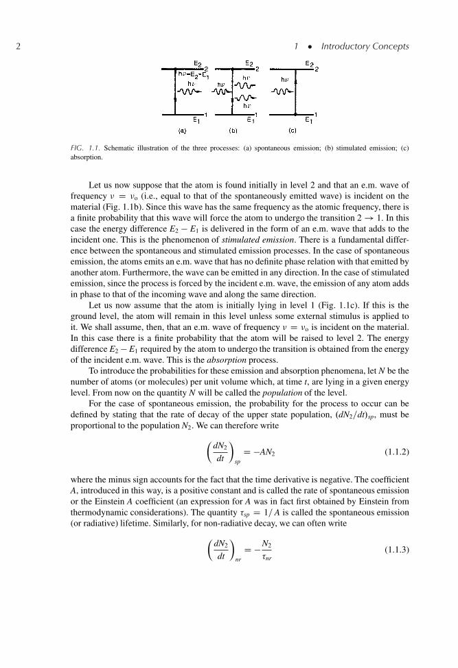
To describe the phenomenon of spontaneous emission, let us consider two energy lev-els, 1 and 2, of some atom or molecule of a given material, their energies being E1 andE2 .E1 < E2/ (Fig. 1.1a). As far as the following discussion is concerned, the two levels couldbe any two out of the infinite set of levels possessed by the atom. It is convenient, however, totake level 1 to be the ground level. Let us now assume that the atom is initially in level 2. SinceE2 > E1, the atom will tend to decay to level 1. The corresponding energy difference, E2 �E1,must therefore be released by the atom. When this energy is delivered in the form of an elec-tromagnetic (e.m. from now on) wave, the process will be called spontaneous (or radiative)emission. The frequency �0 of the radiated wave is then given by the well known expression
�0 D .E2 � E1/=h (1.1.1)
where h is Planck’s constant. Spontaneous emission is therefore characterized by the emis-sion of a photon of energy h�0 D E2 � E1, when the atom decays from level 2 to level 1(Fig. 1.1a). Note that radiative emission is just one of the two possible ways for the atomto decay. The decay can also occur in a nonradiative way. In this case the energy differenceE2 � E1 is delivered in some form of energy other than e.m. radiation (e.g. it may go intokinetic or internal energy of the surrounding atoms or molecules). This phenomenon is callednon-radiative decay.
O. Svelto, Principles of Lasers,c
1DOI: 10.1007/978-1-4419-1302-9 1, � Springer Science+Business Media LLC 2010
2 1 � Introductory Concepts
FIG. 1.1. Schematic illustration of the three processes: (a) spontaneous emission; (b) stimulated emission; (c)absorption.
Let us now suppose that the atom is found initially in level 2 and that an e.m. wave offrequency � D �o (i.e., equal to that of the spontaneously emitted wave) is incident on thematerial (Fig. 1.1b). Since this wave has the same frequency as the atomic frequency, there isa finite probability that this wave will force the atom to undergo the transition 2 ! 1. In thiscase the energy difference E2 � E1 is delivered in the form of an e.m. wave that adds to theincident one. This is the phenomenon of stimulated emission. There is a fundamental differ-ence between the spontaneous and stimulated emission processes. In the case of spontaneousemission, the atoms emits an e.m. wave that has no definite phase relation with that emitted byanother atom. Furthermore, the wave can be emitted in any direction. In the case of stimulatedemission, since the process is forced by the incident e.m. wave, the emission of any atom addsin phase to that of the incoming wave and along the same direction.
Let us now assume that the atom is initially lying in level 1 (Fig. 1.1c). If this is theground level, the atom will remain in this level unless some external stimulus is applied toit. We shall assume, then, that an e.m. wave of frequency � D �o is incident on the material.In this case there is a finite probability that the atom will be raised to level 2. The energydifference E2 � E1 required by the atom to undergo the transition is obtained from the energyof the incident e.m. wave. This is the absorption process.
To introduce the probabilities for these emission and absorption phenomena, let N be thenumber of atoms (or molecules) per unit volume which, at time t, are lying in a given energylevel. From now on the quantity N will be called the population of the level.
For the case of spontaneous emission, the probability for the process to occur can bedefined by stating that the rate of decay of the upper state population, .dN2=dt/sp, must beproportional to the population N2. We can therefore write
�dN2
dt
�sp
D �AN2 (1.1.2)
where the minus sign accounts for the fact that the time derivative is negative. The coefficientA, introduced in this way, is a positive constant and is called the rate of spontaneous emissionor the Einstein A coefficient (an expression for A was in fact first obtained by Einstein fromthermodynamic considerations). The quantity �sp D 1=A is called the spontaneous emission(or radiative) lifetime. Similarly, for non-radiative decay, we can often write
�dN2
dt
�nr
D � N2
�nr(1.1.3)
1.1 � Spontaneous and Stimulated Emission, Absorption 3
where �nr is referred to as the non-radiative decay lifetime. Note that, for spontaneous emis-sion, the numerical value of A (and �sp) depends only on the particular transition considered.For non-radiative decay, � nr depends not only on the transition but also on the characteristicsof the surrounding medium.
We can now proceed, in a similar way, for the stimulated processes (emission orabsorption). For stimulated emission we can write
�dN2
dt
�st
D �W21N2 (1.1.4)
where .dN2=dt/st is the rate at which transitions 2 ! 1 occur as a result of stimulated emissionand W21 is called the rate of stimulated emission. Just as in the case of the A coefficient definedby Eq. (1.1.2) the coefficient W21 also has the dimension of .time/�1. Unlike A, however, W21
depends not only on the particular transition but also on the intensity of the incident e.m.wave. More precisely, for a plane wave, it will be shown that we can write
W21 D �21F (1.1.5)
where F is the photon flux of the wave and �21 is a quantity having the dimension of anarea (the stimulated emission cross section) and depending on the characteristics of the giventransition.
In a similar fashion to Eq. (1.1.4), we can define an absorption rate W21 by means of theequation
�dN1
dt
�a
D �W12N1 (1.1.6)
where .dN1=dt/a is the rate of the 1 ! 2 transitions due to absorption and N1 is the populationof level 1. Furthermore, just as in Eq. (1.1.5), we can write
W12 D �12F (1.1.7)
where �12 is some characteristic area (the absorption cross section), which depends only onthe particular transition.
In what has just been said, the stimulated processes have been characterized by the stim-ulated emission and absorption cross-sections, �21 and �12, respectively. Now, it was shownby Einstein at the beginning of the twentieth century that, if the two levels are non-degenerate,one always has W21 D W12 and �21 D �12. If levels 1 and 2 are g1-fold and g2-fold degenerate,respectively one has instead
g2W21 D g1W12 (1.1.8)
i.e.g2�21 D g1�12 (1.1.9)
Note also that the fundamental processes of spontaneous emission, stimulated emissionand absorption can readily be described in terms of absorbed or emitted photons as follows
4 1 � Introductory Concepts
(see Fig. 1.1). (1) In the spontaneous emission process, the atom decays from level 2 to level 1through the emission of a photon. (2) In the stimulated emission process, the incident photonstimulates the 2 ! 1 transition and we then have two photons (the stimulating plus the stim-ulated one). (3) In the absorption process, the incident photon is simply absorbed to producethe 1 ! 2 transition. Thus we can say that each stimulated emission process creates whileeach absorption process annihilates a photon.
1.2. THE LASER IDEA
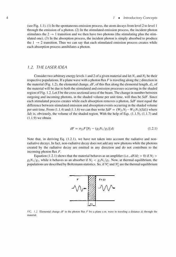
Consider two arbitrary energy levels 1 and 2 of a given material and let N1 and N2 be theirrespective populations. If a plane wave with a photon flux F is traveling along the z direction inthe material (Fig. 1.2), the elemental change, dF, of this flux along the elemental length, dz, ofthe material will be due to both the stimulated and emission processes occurring in the shadedregion of Fig. 1.2. Let S be the cross sectional area of the beam. The change in number betweenoutgoing and incoming photons, in the shaded volume per unit time, will thus be SdF. Sinceeach stimulated process creates while each absorption removes a photon, SdF must equal thedifference between stimulated emission and absorption events occurring in the shaded volumeper unit time. From (1.1.4) and (1.1.6) we can thus write SdF D .W21N2 �W12N1/.Sdz/ whereSdz is, obviously, the volume of the shaded region. With the help of Eqs. (1.1.5), (1.1.7) and(1.1.9) we obtain
dF D �21F ŒN2 � .g2N1=g1/� dz (1.2.1)
Note that, in deriving Eq. (1.2.1), we have not taken into account the radiative and non-radiative decays. In fact, non-radiative decay does not add any new photons while the photonscreated by the radiative decay are emitted in any direction and do not contribute to theincoming photon flux F.
Equation (1.2.1) shows that the material behaves as an amplifier (i.e., dF/dz > 0) if N2 >
g2N1=g1, while it behaves as an absorber if N2 < g2N1=g1. Now, at thermal equilibrium, thepopulations are described by Boltzmann statistics. So, if Ne
1 and Ne2 are the thermal equilibrium
FIG. 1.2. Elemental change dF in the photon flux F fro a plane e.m. wave in traveling a distance dz through thematerial.
1.2 � The Laser Idea 5
populations of the two levels, we have
Ne2
Ne1
D g2
g1exp �
�E2 � E1
kT
�(1.2.2)
where k is Boltzmann’s constant and T the absolute temperature of the material. In thermalequilibrium we thus have Ne
2 < g2Ne1=g1. According to Eq. (1.2.1), the material then acts as
an absorber at frequency �. This is what happens under ordinary conditions. If, however, anon-equilibrium condition is achieved for which N2 > g2N1=g1 then the material will act asan amplifier. In this case we will say that there exists a population inversion in the material,by which we mean that the population difference N2 � .g2N1=g1/ is opposite in sign to thatwhich exists under thermodynamic equilibrium ŒN2 � .g2N1=g1/ < 0�. A material in whichthis population inversion is produced will be called an active material.
If the transition frequency �0 D .E2 � E1/= kT falls in the microwave region, this typeof amplifier is called a maser amplifier. The word maser is an acronym for “microwaveamplification by stimulated emission of radiation.” If the transition frequency falls in theoptical region, the amplifier is called a laser amplifier. The word laser is again an acronym,with the letter l (light) substituted for the letter m (microwave).
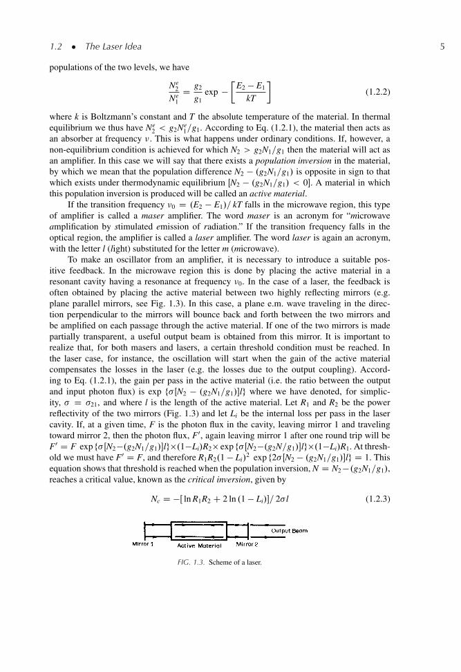
To make an oscillator from an amplifier, it is necessary to introduce a suitable pos-itive feedback. In the microwave region this is done by placing the active material in aresonant cavity having a resonance at frequency �0. In the case of a laser, the feedback isoften obtained by placing the active material between two highly reflecting mirrors (e.g.plane parallel mirrors, see Fig. 1.3). In this case, a plane e.m. wave traveling in the direc-tion perpendicular to the mirrors will bounce back and forth between the two mirrors andbe amplified on each passage through the active material. If one of the two mirrors is madepartially transparent, a useful output beam is obtained from this mirror. It is important torealize that, for both masers and lasers, a certain threshold condition must be reached. Inthe laser case, for instance, the oscillation will start when the gain of the active materialcompensates the losses in the laser (e.g. the losses due to the output coupling). Accord-ing to Eq. (1.2.1), the gain per pass in the active material (i.e. the ratio between the outputand input photon flux) is exp f�ŒN2 � .g2N1=g1/�lg where we have denoted, for simplic-ity, � D �21, and where l is the length of the active material. Let R1 and R2 be the powerreflectivity of the two mirrors (Fig. 1.3) and let Li be the internal loss per pass in the lasercavity. If, at a given time, F is the photon flux in the cavity, leaving mirror 1 and travelingtoward mirror 2, then the photon flux, F0, again leaving mirror 1 after one round trip will beF0 D F exp f�ŒN2�.g2N1=g1/�lg�.1�Li/R2� exp f�ŒN2�.g2N=g1/�lg�.1�Li/R1. At thresh-old we must have F0 D F, and therefore R1R2.1 � Li/
2 exp f2�ŒN2 � .g2N1=g1/�lg D 1. Thisequation shows that threshold is reached when the population inversion, N D N2 �.g2N1=g1/,reaches a critical value, known as the critical inversion, given by
Nc D �Œ ln R1R2 C 2 ln .1 � Li/�= 2� l (1.2.3)
FIG. 1.3. Scheme of a laser.
6 1 � Introductory Concepts
The previous expression can be put in a somewhat simpler form if we define
�1 D � ln R1 D � ln .1 � T1/ (1.2.4a)
�2 D � ln R2 D � ln .1 � T2/ (1.2.4b)
�i D � ln .1 � Li/ (1.2.4c)
where T1 and T2 are the two mirror transmissions (for simplicity mirror absorption has beenneglected). The substitution of Eq. (1.2.4) in Eq. (1.2.3) gives
Nc D �=� l (1.2.5)
where we have defined
� D �i C .�1 C �2/= 2 (1.2.6)
Note that the quantities �i, defined by Eq. (1.2.4c), may be called the logarithmic internal lossof the cavity. In fact, when Li � 1 as usually occurs, one has �i Š Li. Similarly, since both T1
and T2 represent a loss for the cavity, �1 and �2, defined by Eq. (1.2.4a and b), may be calledthe logarithmic losses of the two cavity mirrors. Thus, the quantity � defined by Eq. (1.2.6)will be called the single pass loss of the cavity.
Once the critical inversion is reached, oscillation will build up from spontaneous emis-sion. The photons that are spontaneously emitted along the cavity axis will, in fact, initiatethe amplification process. This is the basis of a laser oscillator, or laser, as it is more simplycalled. Note that, according to the meaning of the acronym laser as discussed above, the wordshould be reserved for lasers emitting visible radiation. The same word is, however, now com-monly applied to any device emitting stimulated radiation, whether in the far or near infrared,ultraviolet, or even in the X-ray region. To be specific about the kind of radiation emitted onethen usually talks about infrared, visible, ultraviolet or X-ray lasers, respectively.
1.3. PUMPING SCHEMES
We will now consider the problem of how a population inversion can be produced in agiven material. At first sight, it might seem that it would be possible to achieve this throughthe interaction of the material with a sufficiently strong e.m. wave, perhaps coming from asufficiently intense lamp, at the frequency � D �o. Since, at thermal equilibrium, one hasg1N1 > g2N2g1, absorption will in fact predominate over stimulated emission. The incomingwave would produce more transitions 1 ! 2 than transitions 2 ! 1 and we would hopein this way to end up with a population inversion. We see immediately, however, that such asystem would not work (at least in the steady state). When in fact the condition is reached suchthat g2N2 D g1N1, then the absorption and stimulated emission processes will compensate oneanother and, according to Eq. (1.2.1), the material will then become transparent. This situationis often referred to as two-level saturation.
1.3 � Pumping Schemes 7
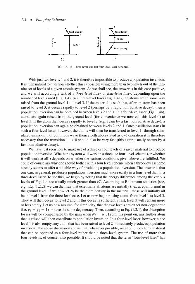
FIG. 1.4. (a) Three-level and (b) four-level laser schemes.
With just two levels, 1 and 2, it is therefore impossible to produce a population inversion.It is then natural to question whether this is possible using more than two levels out of the infi-nite set of levels of a given atomic system. As we shall see, the answer is in this case positive,and we will accordingly talk of a three-level laser or four-level laser, depending upon thenumber of levels used (Fig. 1.4). In a three-level laser (Fig. 1.4a), the atoms are in some wayraised from the ground level 1 to level 3. If the material is such that, after an atom has beenraised to level 3, it decays rapidly to level 2 (perhaps by a rapid nonradiative decay), then apopulation inversion can be obtained between levels 2 and 1. In a four-level laser (Fig. 1.4b),atoms are again raised from the ground level (for convenience we now call this level 0) tolevel 3. If the atom then decays rapidly to level 2 (e.g. again by a fast nonradiative decay), apopulation inversion can again be obtained between levels 2 and 1. Once oscillation starts insuch a four-level laser, however, the atoms will then be transferred to level 1, through stim-ulated emission. For continuos wave (henceforth abbreviated as cw) operation it is thereforenecessary that the transition 1 ! 0 should also be very fast (this again usually occurs by afast nonradiative decay).
We have just seen how to make use of a three or four levels of a given material to producepopulation inversion. Whether a system will work in a three- or four-level scheme (or whetherit will work at all!) depends on whether the various conditions given above are fulfilled. Wecould of course ask why one should bother with a four level scheme when a three-level schemealready seems to offer a suitable way of producing a population inversion. The answer is thatone can, in general, produce a population inversion much more easily in a four-level than in athree-level laser. To see this, we begin by noting that the energy difference among the variouslevels of Fig. 1.4 are usually much greater than kT. According to Boltzmann statistics [see,e.g., Eq. (1.2.2)] we can then say that essentially all atoms are initially (i.e., at equilibrium) inthe ground level. If we now let Nt be the atom density in the material, these will initially allbe in level 1 from the three-level case. Let us now begin raising atoms from level 1 to level 3.They will then decay to level 2 and, if this decay is sufficiently fast, level 3 will remain moreor less empty. Let us now assume, for simplicity, that the two levels are either non-degenerate(i.e. g1 D g2 D 1) or have the same degeneracy. Then, according to Eq. (1.2.1), the absorptionlosses will be compensated by the gain when N2 D N1. From this point on, any further atomthat is raised will then contribute to population inversion. In a four-level laser, however, sincelevel 1 is also empty, any atom that has been raised to level 2 immediately produces populationinversion. The above discussion shows that, whenever possible, we should look for a materialthat can be operated as a four-level rather than a three-level system. The use of more thanfour levels is, of course, also possible. It should be noted that the term “four-level laser” has
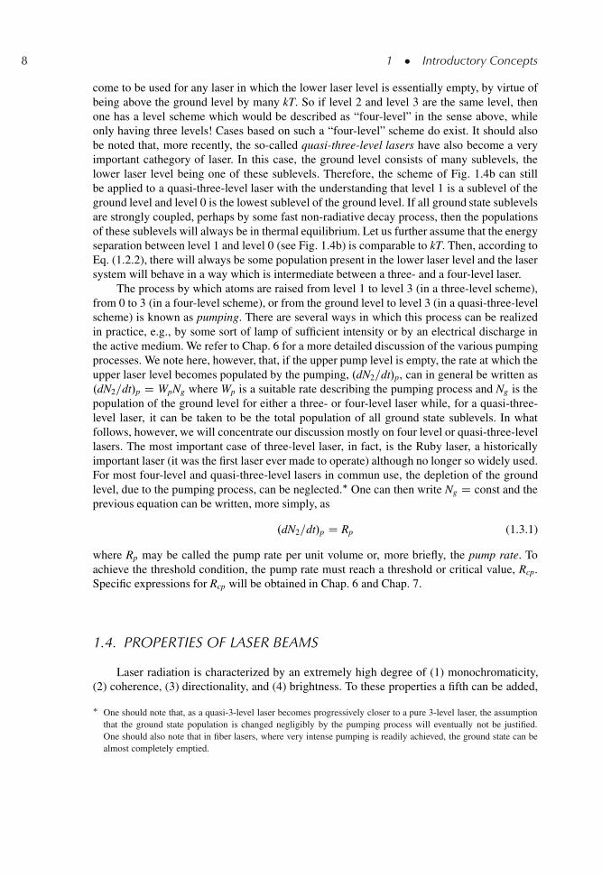
8 1 � Introductory Concepts
come to be used for any laser in which the lower laser level is essentially empty, by virtue ofbeing above the ground level by many kT. So if level 2 and level 3 are the same level, thenone has a level scheme which would be described as “four-level” in the sense above, whileonly having three levels! Cases based on such a “four-level” scheme do exist. It should alsobe noted that, more recently, the so-called quasi-three-level lasers have also become a veryimportant cathegory of laser. In this case, the ground level consists of many sublevels, thelower laser level being one of these sublevels. Therefore, the scheme of Fig. 1.4b can stillbe applied to a quasi-three-level laser with the understanding that level 1 is a sublevel of theground level and level 0 is the lowest sublevel of the ground level. If all ground state sublevelsare strongly coupled, perhaps by some fast non-radiative decay process, then the populationsof these sublevels will always be in thermal equilibrium. Let us further assume that the energyseparation between level 1 and level 0 (see Fig. 1.4b) is comparable to kT. Then, according toEq. (1.2.2), there will always be some population present in the lower laser level and the lasersystem will behave in a way which is intermediate between a three- and a four-level laser.
The process by which atoms are raised from level 1 to level 3 (in a three-level scheme),from 0 to 3 (in a four-level scheme), or from the ground level to level 3 (in a quasi-three-levelscheme) is known as pumping. There are several ways in which this process can be realizedin practice, e.g., by some sort of lamp of sufficient intensity or by an electrical discharge inthe active medium. We refer to Chap. 6 for a more detailed discussion of the various pumpingprocesses. We note here, however, that, if the upper pump level is empty, the rate at which theupper laser level becomes populated by the pumping, .dN2=dt/p, can in general be written as.dN2=dt/p D WpNg where Wp is a suitable rate describing the pumping process and Ng is thepopulation of the ground level for either a three- or four-level laser while, for a quasi-three-level laser, it can be taken to be the total population of all ground state sublevels. In whatfollows, however, we will concentrate our discussion mostly on four level or quasi-three-levellasers. The most important case of three-level laser, in fact, is the Ruby laser, a historicallyimportant laser (it was the first laser ever made to operate) although no longer so widely used.For most four-level and quasi-three-level lasers in commun use, the depletion of the groundlevel, due to the pumping process, can be neglected.� One can then write Ng D const and theprevious equation can be written, more simply, as
.dN2=dt/p D Rp (1.3.1)
where Rp may be called the pump rate per unit volume or, more briefly, the pump rate. Toachieve the threshold condition, the pump rate must reach a threshold or critical value, Rcp.Specific expressions for Rcp will be obtained in Chap. 6 and Chap. 7.
1.4. PROPERTIES OF LASER BEAMS
Laser radiation is characterized by an extremely high degree of (1) monochromaticity,(2) coherence, (3) directionality, and (4) brightness. To these properties a fifth can be added,
� One should note that, as a quasi-3-level laser becomes progressively closer to a pure 3-level laser, the assumptionthat the ground state population is changed negligibly by the pumping process will eventually not be justified.One should also note that in fiber lasers, where very intense pumping is readily achieved, the ground state can bealmost completely emptied.
1.4 � Properties of Laser Beams 9
viz., (5) short time duration. This refers to the capability for producing very short light pulses,a property that, although perhaps less fundamental, is nevertheless very important. We shallnow consider these properties in some detail.
1.4.1. Monochromaticity
Briefly, we can say that this property is due to the following two circumstances: (1) Onlyan e.m. wave of frequency �0 given by (1.1.1) can be amplified. (2) Since the two-mirrorarrangement forms a resonant cavity, oscillation can occur only at the resonance frequenciesof this cavity. The latter circumstance leads to the laser linewidth being often much narrower(by as much as to ten orders of magnitude!) than the usual linewidth of the transition 2 ! 1as observed in spontaneous emission.
1.4.2. Coherence
To first order, for any e.m. wave, one can introduce two concepts of coherence, namely,spatial and temporal coherence.
To define spatial coherence, let us consider two points P1 and P2 that, at time t D 0, lieon the same wave-front of some given e.m. wave and let E1.t/ and E2.t/ be the correspondingelectric fields at these two points. By definition, the difference between the phases of the twofield at time t D 0 is zero. Now, if this difference remains zero at any time t > 0, we willsay that there is a perfect coherence between the two points. If this occurs for any two pointsof the e.m. wave-front, we will say that the wave has perfect spatial coherence. In practice,for any point P1, the point P2 must lie within some finite area around P1 if we want to have agood phase correlation. In this case we will say that the wave has a partial spatial coherenceand, for any point P, we can introduce a suitably defined coherence area Sc.P/.
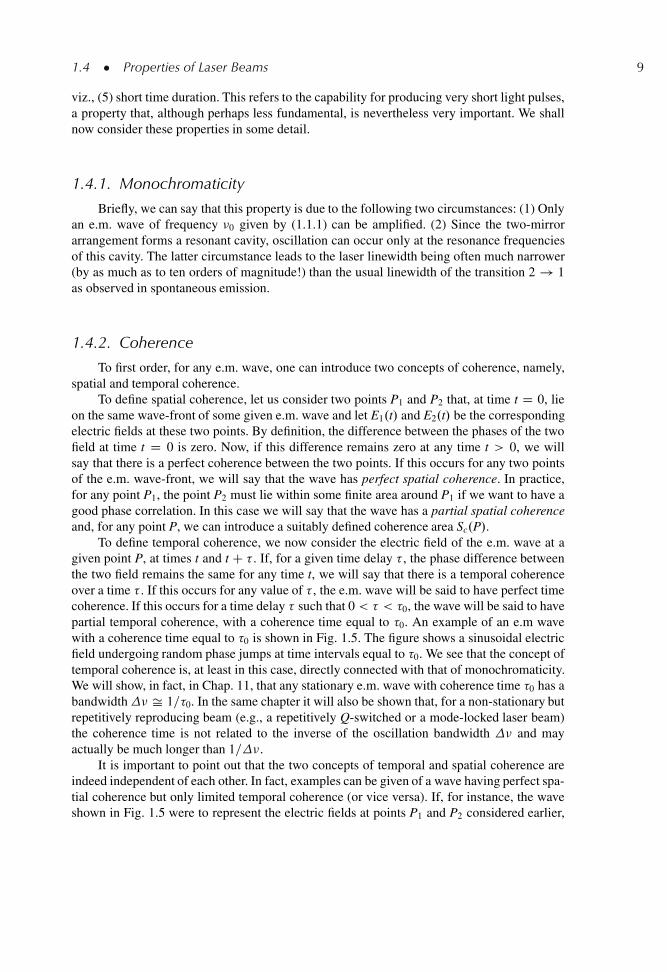
To define temporal coherence, we now consider the electric field of the e.m. wave at agiven point P, at times t and t C � . If, for a given time delay � , the phase difference betweenthe two field remains the same for any time t, we will say that there is a temporal coherenceover a time � . If this occurs for any value of � , the e.m. wave will be said to have perfect timecoherence. If this occurs for a time delay � such that 0 < � < �0, the wave will be said to havepartial temporal coherence, with a coherence time equal to �0. An example of an e.m wavewith a coherence time equal to �0 is shown in Fig. 1.5. The figure shows a sinusoidal electricfield undergoing random phase jumps at time intervals equal to �0. We see that the concept oftemporal coherence is, at least in this case, directly connected with that of monochromaticity.We will show, in fact, in Chap. 11, that any stationary e.m. wave with coherence time �0 has abandwidth� Š 1=�0. In the same chapter it will also be shown that, for a non-stationary butrepetitively reproducing beam (e.g., a repetitively Q-switched or a mode-locked laser beam)the coherence time is not related to the inverse of the oscillation bandwidth � and mayactually be much longer than 1=�.
It is important to point out that the two concepts of temporal and spatial coherence areindeed independent of each other. In fact, examples can be given of a wave having perfect spa-tial coherence but only limited temporal coherence (or vice versa). If, for instance, the waveshown in Fig. 1.5 were to represent the electric fields at points P1 and P2 considered earlier,
10 1 � Introductory Concepts
FIG. 1.5. Example of an e.m. wave with a coherence time of approximately �0.
the spatial coherence between these two points would be complete still the wave having alimited temporal coherence.
We conclude this section by emphasizing that the concepts of spatial and temporal coher-ence provide only a first-order description of the laser’s coherence. Higher order coherenceproperties will in fact discussed in Chap. 11. Such a discussion is essential for a full apprecia-tion of the difference between an ordinary light source and a laser. It will be shown in fact that,by virtue of the differences between the corresponding higher-order coherence properties, alaser beam is fundamentally different from an ordinary light source.
1.4.3. Directionality
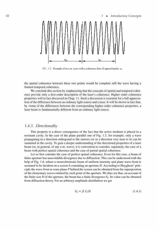
This property is a direct consequence of the fact that the active medium is placed in aresonant cavity. In the case of the plane parallel one of Fig. 1.3, for example, only a wavepropagating in a direction orthogonal to the mirrors (or in a direction very near to it) can besustained in the cavity. To gain a deeper understanding of the directional properties of a laserbeam (or, in general, of any e.m. wave), it is convenient to consider, separately, the case of abeam with perfect spatial coherence and the case of partial spatial coherence.
Let us first consider the case of perfect spatial coherence. Even for this case, a beam offinite aperture has unavoidable divergence due to diffraction. This can be understood with thehelp of Fig. 1.6, where a monochromatic beam of uniform intensity and plane wave-front isassumed to be incident on a screen S containing an aperture D. According to Huyghens’ prin-ciple the wave-front at some plane P behind the screen can be obtained from the superpositionof the elementary waves emitted by each point of the aperture. We thus see that, on account ofthe finite size D of the aperture, the beam has a finite divergence d. Its value can be obtainedfrom diffraction theory. For an arbitrary amplitude distribution we get
d D ˇ �=D (1.4.1)
1.4 � Properties of Laser Beams 11
FIG. 1.6. Divergence of a plane e.m. wave due to diffraction.
where � and D are the wavelength and the diameter of the beam. The factor ˇ is a numericalcoefficient of the order of unity whose value depends on the shape of the amplitude distribu-tion and on the way in which both the divergence and the beam diameter are defined. A beamwhose divergence can be expressed as in Eq. (1.4.1) is described as being diffraction limited.
If the wave has only a partial spatial coherence, its divergence will be larger than theminimum value set by diffraction. Indeed, for any point P0 of the wave-front, the Huygens’argument of Fig. 1.6 can only be applied for points lying within the coherence area Sc aroundpoint P0. The coherence area thus acts as a limiting aperture for the coherent superposition ofthe elementary wavelets. The beam divergence will now be given by
D ˇ�= ŒSc�1=2 (1.4.2)
where. again, ˇ is a numerical coefficient of the order of unity whose exact value depends onthe way in which both the divergence and the coherence area Sc are defined.
We conclude this general discussion of the directional properties of e.m. waves by point-ing out that, given suitable operating conditions, the output beam of a laser can be madediffraction limited.
1.4.4. Brightness
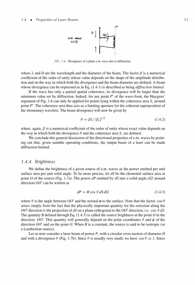
We define the brightness of a given source of e.m. waves as the power emitted per unitsurface area per unit solid angle. To be more precise, let dS be the elemental surface area atpoint O of the source (Fig. 1.7a). The power dP emitted by dS into a solid angle d˝ arounddirection OO0 can be written as
dP D B cos dS d� (1.4.3)
where is the angle between OO0 and the normal n to the surface. Note that the factor cos arises simply from the fact that the physically important quantity for the emission along theOO0 direction is the projection of dS on a plane orthogonal to the OO0 direction, i.e. cos dS.The quantity B defined through Eq. (1.4.3) is called the source brightness at the point O in thedirection OO0. This quantity will generally depend on the polar coordinates and � of thedirection OO0 and on the point O. When B is a constant, the source is said to be isotropic (ora Lambertian source).
Let us now consider a laser beam of power P, with a circular cross section of diameter Dand with a divergence (Fig. 1.7b). Since is usually very small, we have cos Š 1. Since
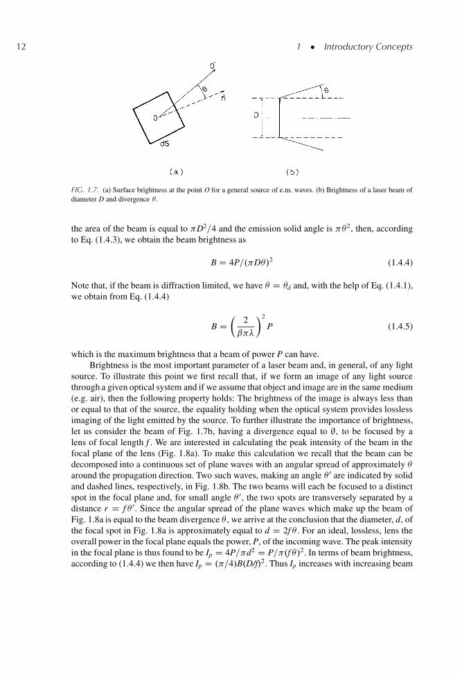
12 1 � Introductory Concepts
FIG. 1.7. (a) Surface brightness at the point O for a general source of e.m. waves. (b) Brightness of a laser beam ofdiameter D and divergence .
the area of the beam is equal to D2=4 and the emission solid angle is 2, then, accordingto Eq. (1.4.3), we obtain the beam brightness as
B D 4P=. D/2 (1.4.4)
Note that, if the beam is diffraction limited, we have D d and, with the help of Eq. (1.4.1),we obtain from Eq. (1.4.4)
B D�
2
ˇ �
�2
P (1.4.5)
which is the maximum brightness that a beam of power P can have.Brightness is the most important parameter of a laser beam and, in general, of any light
source. To illustrate this point we first recall that, if we form an image of any light sourcethrough a given optical system and if we assume that object and image are in the same medium(e.g. air), then the following property holds: The brightness of the image is always less thanor equal to that of the source, the equality holding when the optical system provides losslessimaging of the light emitted by the source. To further illustrate the importance of brightness,let us consider the beam of Fig. 1.7b, having a divergence equal to θ, to be focused by alens of focal length f . We are interested in calculating the peak intensity of the beam in thefocal plane of the lens (Fig. 1.8a). To make this calculation we recall that the beam can bedecomposed into a continuous set of plane waves with an angular spread of approximately around the propagation direction. Two such waves, making an angle 0 are indicated by solidand dashed lines, respectively, in Fig. 1.8b. The two beams will each be focused to a distinctspot in the focal plane and, for small angle 0, the two spots are transversely separated by adistance r D f 0. Since the angular spread of the plane waves which make up the beam ofFig. 1.8a is equal to the beam divergence , we arrive at the conclusion that the diameter, d, ofthe focal spot in Fig. 1.8a is approximately equal to d D 2f . For an ideal, lossless, lens theoverall power in the focal plane equals the power, P, of the incoming wave. The peak intensityin the focal plane is thus found to be Ip D 4P= d2 D P= .f /2. In terms of beam brightness,according to (1.4.4) we then have Ip D . =4/B.D/f/2. Thus Ip increases with increasing beam
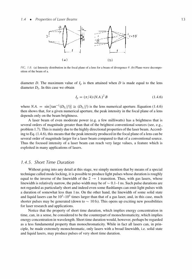
1.4 � Properties of Laser Beams 13
FIG. 1.8. (a) Intensity distribution in the focal plane of a lens for a beam of divergence . (b) Plane-wave decompo-sition of the beam of a.
diameter D. The maximum value of Ip is then attained when D is made equal to the lensdiameter DL. In this case we obtain
Ip D . =4/ .N.A./2 B (1.4.6)
where N.A. D sin Œ tan�1.DL=f /� Š .DL=f / is the lens numerical aperture. Equation (1.4.6)then shows that, for a given numerical aperture, the peak intensity in the focal plane of a lensdepends only on the beam brightness.
A laser beam of even moderate power (e.g. a few milliwatts) has a brightness that isseveral orders of magnitude greater than that of the brightest conventional sources (see, e.g.,problem 1.7). This is mainly due to the highly directional properties of the laser beam. Accord-ing to Eq. (1.4.6), this means that the peak intensity produced in the focal plane of a lens can beseveral order of magnitude larger for a laser beam compared to that of a conventional source.Thus the focused intensity of a laser beam can reach very large values, a feature which isexploited in many applications of lasers.
1.4.5. Short Time Duration
Without going into any detail at this stage, we simply mention that by means of a specialtechnique called mode locking, it is possible to produce light pulses whose duration is roughlyequal to the inverse of the linewidth of the 2 ! 1 transition. Thus, with gas lasers, whoselinewidth is relatively narrow, the pulse-width may be of � 0.1–1 ns. Such pulse durations arenot regarded as particularly short and indeed even some flashlamps can emit light pulses witha duration of somewhat less than 1 ns. On the other hand, the linewidth of some solid stateand liquid lasers can be 103–105 times larger than that of a gas laser, and, in this case, muchshorter pulses may be generated (down to � 10 fs). This opens up exciting new possibilitiesfor laser research and applications.
Notice that the property of short time duration, which implies energy concentration intime, can, in a sense, be considered to be the counterpart of monochromaticity, which impliesenergy concentration in wavelength. Short time duration would, however, perhaps be regardedas a less fundamental property than monochromaticity. While in fact all lasers can, in prin-ciple, be made extremely monochromatic, only lasers with a broad linewidth, i.e. solid stateand liquid lasers, may produce pulses of very short time duration.
14 1 � Introductory Concepts
1.5. TYPES OF LASERS
The various types of laser that have been developed so far, display a very wide rangeof physical and operating parameters. Indeed, if lasers are characterized according to thephysical state of the active material, one uses the description of solid state, liquid or gas lasers.A rather special case is where the active material consists of free electrons, at relativisticvelocities, passing through a spatially periodic magnetic field (free-electron lasers). If lasersare characterized by the wavelength of the emitted radiation, one refers to infrared lasers,visible lasers, UV and X-ray lasers. The corresponding wavelength may range from � 1 mm(i.e. millimeter waves) down to � 1 nm (i.e. to the upper limit of hard X-rays). The span inwavelength can thus be a factor of � 106 (we recall that the visible range spans less than afactor 2, roughly from 700 to 400 nm). Output powers cover an even larger range of values.For cw lasers, typical powers go from a few mW, in lasers used for signal sources (e.g. foroptical communications or for bar-code scanners), to tens of kW in lasers used for materialworking, to a few MW (� 5 MW so far) in lasers required for some military applications (e.g.for directed energy weapons). For pulsed lasers the peak power can be much higher than forcw lasers and can reach values as high as 1 PW .1015 W/! Again for pulsed lasers, the pulseduration can vary widely from the ms level typical of lasers operating in the so-called free-running regime (i.e. without any Q-switching or mode-locking element in the cavity) down toabout 10 fs .1 fs D 10�15 s/ for some mode locked lasers. The physical dimensions can alsovary widely. In terms of cavity length, for instance, the length can be as small as � 1 μm forthe shortest lasers up to some km for the longest (e.g. a laser 6.5 km long, which was set up ina cave for geodetic studies).
This wide range of physical or operating parameters represent both a strength and aweakness. As far as applications are concerned, this wide range of parameters offers enormouspotential in several fields of fundamental and applied sciences. On the other hand, in termsof markets, a very wide spread of different devices and systems can be an obstacle to massproduction and its associated price reduction.
1.6. ORGANIZATION OF THE BOOK
The organization of the book is based on the fact that, as indicated in our discussionso far, a laser can be considered to consist of three elements: (1) an active material, (2) apumping scheme, (3) a resonator. Accordingly, the next two chapters deal with the interactionof radiation with matter, starting from the simplest cases, i.e. atoms or ions in an essentiallyisolated situation, (Chap. 2), and going on to the more complicated cases, i.e. moleculesand semiconductors, (Chap. 3). As an introduction to optical resonators, the next Chapter(Chap. 4) considers some topics relating to ray and wave propagation in particular opticalelements such as free-space, optical lens-like media, Fabry-Perot interferometers and multi-layer dielectric coatings. Chapter 5 then deals with the theory of optical resonators while thenext Chapter (Chap. 6) deals with the pumping processes. The concepts introduced in thesechapters are then used in next two chapters (Chap. 7 and 8) where the theory is developedfor continuous wave and transient laser behavior, respectively. The theory is based on thelowest order approximation, i.e. using the rate equation approach. This treatment is, in fact,
Problems 15
capable of describing most laser characteristics. Obviously, lasers based upon different typesof active media have significant differences in their characteristics. So, the next two chap-ters (Chap. 9 and 10) discuss the characteristic properties of a number of types of laser. ThusChap. 9 covers ionic crystal, dye and semiconductor lasers, these having a number of com-mon features, while Chap. 10 considers gas, chemical and free-electron lasers. By this point,the reader should have acquired sufficient understanding of laser behavior to go on to a studyof the properties of the output beam (coherence, monochromaticity, brightness, noise). Theseproperties are considered in Chap. 11. Finally, the theme of Chap. 12 is based on the fact that,before being put to use, a laser beam is generally transformed in some way. This includes:(1) spatial transformation of the beam due to its propagation through e.g. a lens system; (2)amplitude transformation as a result of passing through an amplifier; (3) wavelength trans-formation, or frequency conversion, via a number of nonlinear phenomena (second harmonicgeneration, parametric processes); (4) time transformation by e.g. pulse compression.
PROBLEMS
1.1. The part of the e.m. spectrum that is of interest in the laser field starts from the submillimiterwave region and goes down in wavelength to the X-ray region. This covers the following regions insuccession: (1) far infrared; (2) near infrared; (3) visible; (4) ultraviolet (uv); (5) vacuum ultraviolet(vuv); (6) soft X-ray; (7) X-ray: From standard textbooks find the wavelength intervals of the aboveregions. Memorize or record these intervals since they are frequently used in this book.
1.2. As a particular case of Problem 1.1, memorize or record the wavelengths corresponding to blue,green, and red light.
1.3. If levels 1 and 2 of Fig. 1.1 are separated by an energy E2�E1 such that the corresponding transitionfrequency falls in the middle of the visible range, calculate the ratio of the populations of the twolevels in thermal equilibrium at room temperature.
1.4. When in thermal equilibrium at T D 300 K, the ratio of the level populations N2=N1 for someparticular pair of levels is given by 1=e. Calculate the frequency � for this transition. In what regionof the e.m. spectrum does this frequency fall?
1.5. A laser cavity consists of two mirrors with reflectivities R1 D 1 and R2 D 0.5 while the internalloss per pass is Li D 1%. Calculate the total logarithmic losses per pass. If the length of the activematerial is l D 7.5 cm and the transition cross section is � D 2.8 � 10�19 cm2, calculate then thethreshold inversion.
1.6. The beam from a ruby laser .� Š 694 nm/ is sent to the moon after passing through a telescopeof 1 m diameter. Calculate the approximate value of beam diameter on the moon assuming thatthe beam has perfect spatial coherence (the distance between earth and moon is approximately384,000 km).
1.7. The brightness of probably the brightest lamp so far available (PEK Labs type 107/109, excitedby 100 W of electrical power) is about 95 W/cm2 sr in its most intense green line .λ D 546 nm/.Compare this brightness with that of a 1 W Argon laser .λ D 514.5 nm/, which can be assumed tobe diffraction limited.
2
Interaction of Radiation with Atomsand Ions
2.1. INTRODUCTION
This chapter deals with the interaction of radiation with atoms and ions which are weaklyinteracting with any surrounding species, such as atoms or ions in a gas phase or impurityions in an ionic crystal. The somewhat more complicated case of interaction of radiationwith molecules or semiconductors will be considered in the next chapter. Since the subjectof radiation interaction with matter is, of course, very wide, we will limit our discussionto those phenomena which are relevant for atoms and ions acting as active media. So, afteran introductory section dealing with the theory of blackbody radiation, a milestone for thewhole of modern physics, we will consider the elementary processes of absorption, stimulatedemission, spontaneous emission, and nonradiative decay. They will first be considered withinthe simplifying assumptions of a dilute medium and a low intensity. Following this, situationsinvolving a high beam intensity and a medium that is not dilute (leading, in particular, to thephenomena of saturation and amplified spontaneous emission) will be considered. A numberof very important, although perhaps less general, topics relating to the photophysics of dyelasers, free-electron lasers, and X-ray lasers will be briefly considered in Chaps. 9 and 10immediately preceding the discussion of the corresponding laser.
2.2. SUMMARY OF BLACKBODY RADIATION THEORY.1/
Let us consider a cavity filled with a homogeneous and isotropic medium. If the walls ofthe cavity are kept at a constant temperature, T, they will continuously emit and receive powerin the form of electromagnetic (e.m.) radiation. When the rates of absorption and emission
O. Svelto, Principles of Lasers,c
17DOI: 10.1007/978-1-4419-1302-9 2, � Springer Science+Business Media LLC 2010
18 2 � Interaction of Radiation with Atoms and Ions
becomes equal, an equilibrium condition is established at the walls of the cavity as well as ateach point of the dielectric. This situation can be described by introducing the energy density�, which represents the electromagnetic energy contained in unit volume of the cavity. Thisenergy density can be expressed as a function of the electric field, E.t/, and magnetic field,H.t/, according to the formula
� D <1
2"E2>C 1
2�H2> (2.2.1)
where " and � are, respectively, the dielectric constant and the magnetic permeability of themedium inside the cavity and where the symbol < > indicates a time average over a cycleof the radiation field. We can then represent the spectral energy distribution of this radiationby the function �� , which is a function of frequency �. This is defined as follows: ��d�represents the energy density of radiation in the frequency range from � to � C d�. Therelationship between � and �� is obviously
� DZ 1
0��d� (2.2.2)
Suppose now that a hole is made in the wall of the cavity. If we let I� be the spectral intensityof the light escaping from the hole, one can show that I� is proportional to �� obeying thesimple relation
I� D .c=4n/�� (2.2.3)
where c is the velocity of light in the vacuum and n is the refractive index of the mediuminside the cavity. We can now show that I� and hence �� are universal functions, independentof either the nature of the walls or the cavity shape, and dependent only on the frequency� and temperature T of the cavity. This property of �� can be proven through the followingsimple thermodynamic argument. Let us suppose we have two cavities of arbitrary shape,whose walls are at the same temperature T. To ensure that the temperature remains constant,we may imagine that the walls of the two cavities are in thermal contact with two thermostatsat temperature T. Let us suppose that, at a given frequency �, the energy density �0
� in thefirst cavity is greater than the corresponding value �00
� in the second cavity. We now opticallyconnect the two cavities by making a hole in each and then imaging, with some optical system,each hole onto the other. We also insert an ideal filter in the optical system, which lets throughonly a small frequency range around the frequency�. If �0
� > �00� then, according to Eq. (2.2.3),
one will have I0� > I00
� and there will be a net flow of electromagnetic energy from cavity 1 tocavity 2. Such a flow of energy, however, would violate the second law of thermodynamics,since the two cavities are at the same temperature. Therefore one must have �0
� D �00� for all
frequencies.The problem of calculating this universal function ��.�, T/ was a very challenging one
for the physicists of the time. Its complete solution was provided by Planck, who, in order tofind a correct solution of the problem, had to introduce the so-called hypothesis of light quanta.The blackbody theory is therefore one of the fundamental bases of modern physics..1/ Beforegoing further into it, we first need to consider the electromagnetic modes of a blackbodycavity. Since the function �� is independent of the cavity shape or the nature of the dielectric
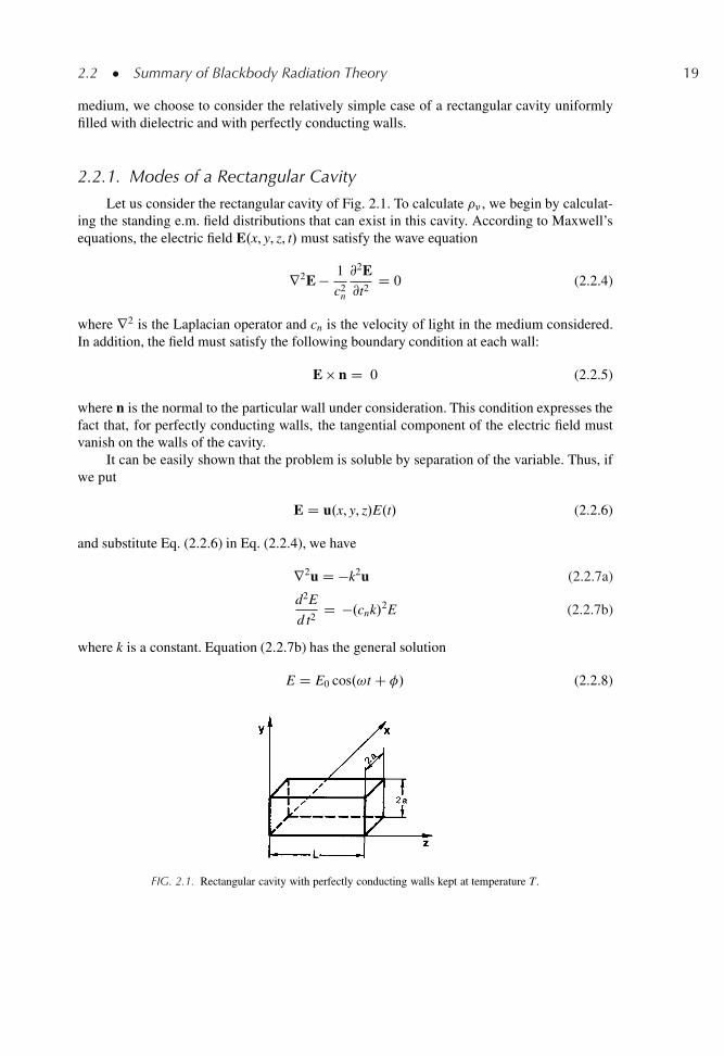
2.2 � Summary of Blackbody Radiation Theory 19
medium, we choose to consider the relatively simple case of a rectangular cavity uniformlyfilled with dielectric and with perfectly conducting walls.
2.2.1. Modes of a Rectangular Cavity
Let us consider the rectangular cavity of Fig. 2.1. To calculate �� , we begin by calculat-ing the standing e.m. field distributions that can exist in this cavity. According to Maxwell’sequations, the electric field E.x, y, z, t/ must satisfy the wave equation
r2E � 1
c2n
@2E@t2
D 0 (2.2.4)
where r2 is the Laplacian operator and cn is the velocity of light in the medium considered.In addition, the field must satisfy the following boundary condition at each wall:
E � n D 0 (2.2.5)
where n is the normal to the particular wall under consideration. This condition expresses thefact that, for perfectly conducting walls, the tangential component of the electric field mustvanish on the walls of the cavity.
It can be easily shown that the problem is soluble by separation of the variable. Thus, ifwe put
E D u.x, y, z/E.t/ (2.2.6)
and substitute Eq. (2.2.6) in Eq. (2.2.4), we have
r2u D �k2u (2.2.7a)
d2E
d t2D �.cnk/2E (2.2.7b)
where k is a constant. Equation (2.2.7b) has the general solution
E D E0 cos.!t C �/ (2.2.8)
FIG. 2.1. Rectangular cavity with perfectly conducting walls kept at temperature T .
20 2 � Interaction of Radiation with Atoms and Ions
where E0 and � are arbitrary constant and where
! D cnk (2.2.9)
With E.t/ given by Eq. (2.2.8), we see that the solution Eq. (2.2.6) can be written as
E.x, y, z, t/ D E0u.x, y, z/ exp.j!t C �/ (2.2.9a)
and thus corresponds to a standing wave configuration of the e.m. field within the cavity. Infact the amplitude of oscillation at a given point of the cavity is constant in time. A solutionof this type is referred to as a an e.m. mode of the cavity.
We are now left with the task of solving Eq. (2.2.7a), known as the Helmholtz equation,subject to the boundary condition given by Eq. (2.2.5). It can readily be verified that theexpressions
ux D ex cos kxx sin kyy sin kzzuy D ey sin kxx cos kyy sin kzzuz D ez sin kxx sin kyy cos kzz
(2.2.10)
satisfy Eq. (2.2.7a) for any value of ex, ey, ez, provided that
k2x C k2
y C k2z D k2 (2.2.11)
Furthermore, the solution Eq. (2.2.10) already satisfies the boundary condition Eq. (2.2.5) onthe three planes x D 0, y D 0, z D 0. If we now impose the condition that Eq. (2.2.5) shouldalso be satisfied on the other walls of the cavity, we obtain
kx D l =2aky D m =2akz D n =L
(2.2.12)
where l, m, and n are positive integers. Their physical significance can be seen immediately:they represent the number of nodes that the standing wave mode has along the directions x, y,and z, respectively. For fixed values of l, m, and n it follows that kx, ky, and kz will also befixed and, according to Eqs. (2.2.9) and (2.2.11), the angular frequency ! of the mode willalso be fixed and given by
!lmn D cn
"�l
2a
�2
C�m
2a
�2 C�n
L
�2#1=2
(2.2.13)
where we have explicitly indicated that the frequency of the mode will depend on the indicesl, m, and n. The mode is still not completely determined, however, since ex, ey, and ez are stillarbitrary. However, Maxwell’s equations provide another condition that must be satisfied bythe electric field, i.e., r � u D 0, from which, with the help of Eq. (2.2.10), we get
e � k D 0 (2.2.14)
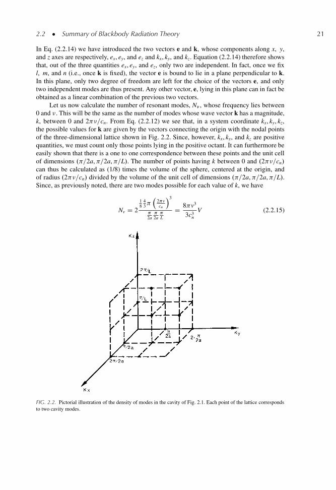
2.2 � Summary of Blackbody Radiation Theory 21
In Eq. (2.2.14) we have introduced the two vectors e and k, whose components along x, y,and z axes are respectively, ex, ey, and ez and kx, ky, and kz. Equation (2.2.14) therefore showsthat, out of the three quantities ex, ey, and ez, only two are independent. In fact, once we fixl, m, and n (i.e., once k is fixed), the vector e is bound to lie in a plane perpendicular to k.In this plane, only two degree of freedom are left for the choice of the vectors e, and onlytwo independent modes are thus present. Any other vector, e, lying in this plane can in fact beobtained as a linear combination of the previous two vectors.
Let us now calculate the number of resonant modes, N� , whose frequency lies between0 and �. This will be the same as the number of modes whose wave vector k has a magnitude,k, between 0 and 2 �=cn. From Eq. (2.2.12) we see that, in a system coordinate kx, ky, kz,the possible values for k are given by the vectors connecting the origin with the nodal pointsof the three-dimensional lattice shown in Fig. 2.2. Since, however, kx, ky, and kz are positivequantities, we must count only those points lying in the positive octant. It can furthermore beeasily shown that there is a one to one correspondence between these points and the unit cellof dimensions . =2a, =2a, =L/. The number of points having k between 0 and .2 �=cn/
can thus be calculated as (1/8) times the volume of the sphere, centered at the origin, andof radius .2 �=cn/ divided by the volume of the unit cell of dimensions . =2a, =2a, =L/.Since, as previously noted, there are two modes possible for each value of k, we have
Nv D 2
18
43 �
2�vcn
�3
�2a
�2a
�L
D 8 v3
3c3n
V (2.2.15)
FIG. 2.2. Pictorial illustration of the density of modes in the cavity of Fig. 2.1. Each point of the lattice correspondsto two cavity modes.
22 2 � Interaction of Radiation with Atoms and Ions
where V is the total volume of the cavity. If we now define p.�/ as the number of modes perunit volume and per unit frequency range, we have
p.�/ D 1
V
dN
d�D 8 �2
c3n
. (2.2.16)
2.2.2. The Rayleigh-Jeans and Planck Radiation Formula
Having calculated the quantity p.�/ we can now proceed to calculate the energy density�� . We can begin by writing �� as the product of the number of modes per unit volume per unitfrequency range, p.�/, multiplied by the average energy<E> contained in each mode, i.e.
�� D p�<E> (2.2.17)
To calculate <E> we assume that the cavity walls are kept at a constant temperature T.According to Boltzmann’s statistics, the probability dp that the energy of a given cavity modelies between E and E C dE is expressed by dp D C expŒ�.E=kT/�dE, where C is a constant tobe established by the condition
R10 C expŒ�.E=kT/dE D 1. The average energy of the mode
<E> is therefore given by
<E> DR1
0 E expŒ�.E=kT/�dER10 expŒ�.E=kT/�dE
D kT (2.2.18)
From Eq. (2.2.16), Eqs. (2.2.17), and (2.2.18) we then get
�� D�
8 �2
c3n
�kT (2.2.19)
This is the well known Rayleigh-Jeans radiation formula. It is, however, in complete disagree-ment with the experimental results. Indeed, it is immediately obvious that Eq. (2.2.19) mustbe wrong since it would imply an infinite total energy density � [see Eq. (2.2.2)]. Equa-tion (2.2.19) does, however, represent the inevitable conclusion of the previous classicalarguments.
The problem remained unsolved until, at the beginning of this century, Planck introducedthe hypothesis of light quanta. The fundamental hypothesis of Planck was that the energy in agiven mode could not have any arbitrary value between 0 and 1, as was implicitly assumedin Eq. (2.2.18), but that the allowed values of this energy should be integral multiples ofa fundamental quantity, proportional to the frequency of the mode. In other words, Planckassumed that the energy of the mode could be written as
E D nh� (2.2.20)
where n is a positive integer and h a constant (which was later called Planck’s constant).Without entering into too many details, here, on this fundamental hypothesis, we merely wishto note that this essentially implies that energy exchange between the inside of the cavity
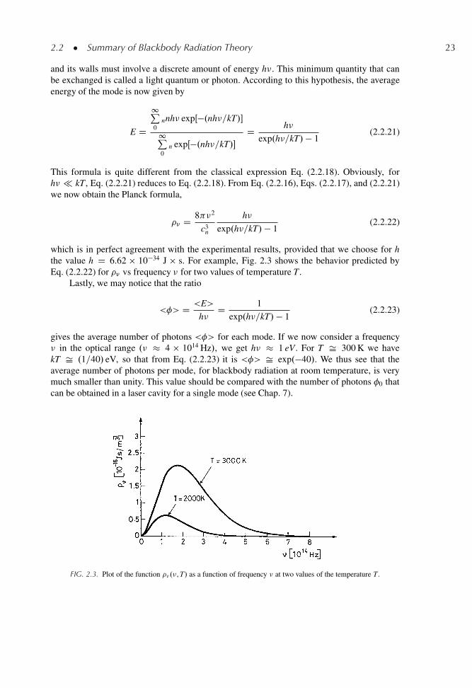
2.2 � Summary of Blackbody Radiation Theory 23
and its walls must involve a discrete amount of energy h�. This minimum quantity that canbe exchanged is called a light quantum or photon. According to this hypothesis, the averageenergy of the mode is now given by
E D
1P0
nnh� expŒ�.nh�=kT/�
1P0
n expŒ�.nh�=kT/�D h�
exp.h�=kT/� 1(2.2.21)
This formula is quite different from the classical expression Eq. (2.2.18). Obviously, forh� � kT, Eq. (2.2.21) reduces to Eq. (2.2.18). From Eq. (2.2.16), Eqs. (2.2.17), and (2.2.21)we now obtain the Planck formula,
�� D 8 �2
c3n
h�
exp.h�=kT/� 1(2.2.22)
which is in perfect agreement with the experimental results, provided that we choose for hthe value h D 6.62 � 10�34 J � s. For example, Fig. 2.3 shows the behavior predicted byEq. (2.2.22) for �� vs frequency � for two values of temperature T.
Lastly, we may notice that the ratio
<�> D <E>
h�D 1
exp.h�=kT/� 1(2.2.23)
gives the average number of photons <�> for each mode. If we now consider a frequency� in the optical range .� � 4 � 1014 Hz/, we get h� � 1 eV . For T Š 300 K we havekT Š .1=40/ eV, so that from Eq. (2.2.23) it is <�> Š exp.�40/. We thus see that theaverage number of photons per mode, for blackbody radiation at room temperature, is verymuch smaller than unity. This value should be compared with the number of photons �0 thatcan be obtained in a laser cavity for a single mode (see Chap. 7).
FIG. 2.3. Plot of the function ��.�, T/ as a function of frequency � at two values of the temperature T .
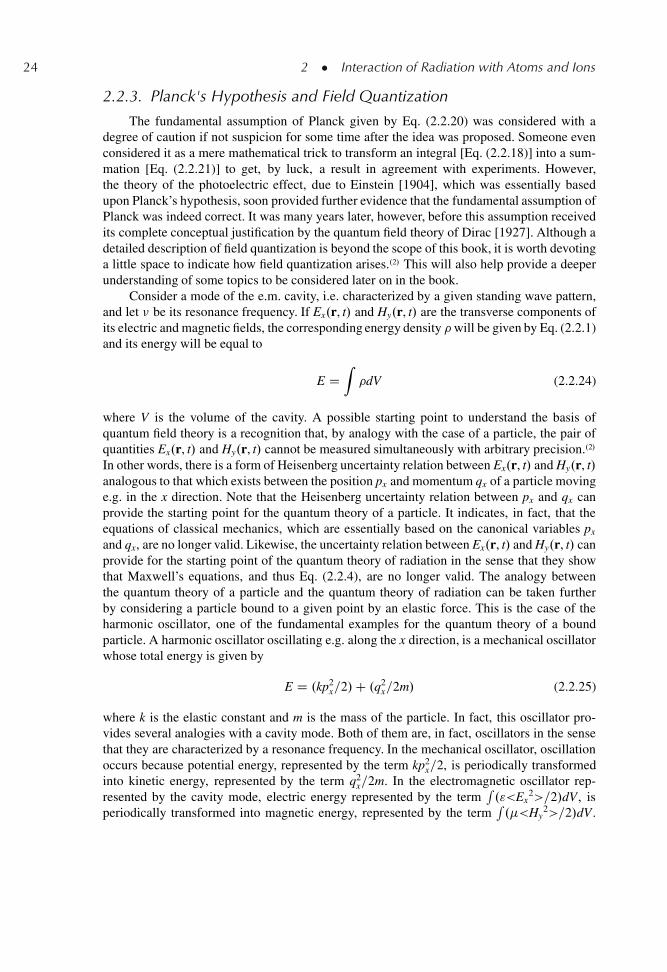
24 2 � Interaction of Radiation with Atoms and Ions
2.2.3. Planck's Hypothesis and Field Quantization
The fundamental assumption of Planck given by Eq. (2.2.20) was considered with adegree of caution if not suspicion for some time after the idea was proposed. Someone evenconsidered it as a mere mathematical trick to transform an integral [Eq. (2.2.18)] into a sum-mation [Eq. (2.2.21)] to get, by luck, a result in agreement with experiments. However,the theory of the photoelectric effect, due to Einstein [1904], which was essentially basedupon Planck’s hypothesis, soon provided further evidence that the fundamental assumption ofPlanck was indeed correct. It was many years later, however, before this assumption receivedits complete conceptual justification by the quantum field theory of Dirac [1927]. Although adetailed description of field quantization is beyond the scope of this book, it is worth devotinga little space to indicate how field quantization arises..2/ This will also help provide a deeperunderstanding of some topics to be considered later on in the book.
Consider a mode of the e.m. cavity, i.e. characterized by a given standing wave pattern,and let � be its resonance frequency. If Ex.r, t/ and Hy.r, t/ are the transverse components ofits electric and magnetic fields, the corresponding energy density �will be given by Eq. (2.2.1)and its energy will be equal to
E DZ�dV (2.2.24)
where V is the volume of the cavity. A possible starting point to understand the basis ofquantum field theory is a recognition that, by analogy with the case of a particle, the pair ofquantities Ex.r, t/ and Hy.r, t/ cannot be measured simultaneously with arbitrary precision..2/
In other words, there is a form of Heisenberg uncertainty relation between Ex.r, t/ and Hy.r, t/analogous to that which exists between the position px and momentum qx of a particle movinge.g. in the x direction. Note that the Heisenberg uncertainty relation between px and qx canprovide the starting point for the quantum theory of a particle. It indicates, in fact, that theequations of classical mechanics, which are essentially based on the canonical variables px
and qx, are no longer valid. Likewise, the uncertainty relation between Ex.r, t/ and Hy.r, t/ canprovide for the starting point of the quantum theory of radiation in the sense that they showthat Maxwell’s equations, and thus Eq. (2.2.4), are no longer valid. The analogy betweenthe quantum theory of a particle and the quantum theory of radiation can be taken furtherby considering a particle bound to a given point by an elastic force. This is the case of theharmonic oscillator, one of the fundamental examples for the quantum theory of a boundparticle. A harmonic oscillator oscillating e.g. along the x direction, is a mechanical oscillatorwhose total energy is given by
E D .kp2x=2/C .q2
x=2m/ (2.2.25)
where k is the elastic constant and m is the mass of the particle. In fact, this oscillator pro-vides several analogies with a cavity mode. Both of them are, in fact, oscillators in the sensethat they are characterized by a resonance frequency. In the mechanical oscillator, oscillationoccurs because potential energy, represented by the term kp2
x=2, is periodically transformedinto kinetic energy, represented by the term q2
x=2m. In the electromagnetic oscillator rep-resented by the cavity mode, electric energy represented by the term
R."<Ex
2>=2/dV , isperiodically transformed into magnetic energy, represented by the term
R.�<Hy
2>=2/dV .
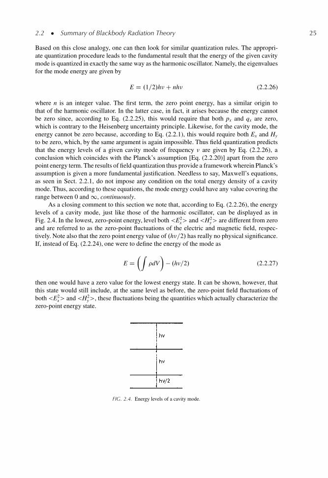
2.2 � Summary of Blackbody Radiation Theory 25
Based on this close analogy, one can then look for similar quantization rules. The appropri-ate quantization procedure leads to the fundamental result that the energy of the given cavitymode is quantized in exactly the same way as the harmonic oscillator. Namely, the eigenvaluesfor the mode energy are given by
E D .1=2/h�C nh� (2.2.26)
where n is an integer value. The first term, the zero point energy, has a similar origin tothat of the harmonic oscillator. In the latter case, in fact, it arises because the energy cannotbe zero since, according to Eq. (2.2.25), this would require that both px and qx are zero,which is contrary to the Heisenberg uncertainty principle. Likewise, for the cavity mode, theenergy cannot be zero because, according to Eq. (2.2.1), this would require both Ex and Hy
to be zero, which, by the same argument is again impossible. Thus field quantization predictsthat the energy levels of a given cavity mode of frequency � are given by Eq. (2.2.26), aconclusion which coincides with the Planck’s assumption [Eq. (2.2.20)] apart from the zeropoint energy term. The results of field quantization thus provide a framework wherein Planck’sassumption is given a more fundamental justification. Needless to say, Maxwell’s equations,as seen in Sect. 2.2.1, do not impose any condition on the total energy density of a cavitymode. Thus, according to these equations, the mode energy could have any value covering therange between 0 and 1, continuously.
As a closing comment to this section we note that, according to Eq. (2.2.26), the energylevels of a cavity mode, just like those of the harmonic oscillator, can be displayed as inFig. 2.4. In the lowest, zero-point energy, level both <E2
x> and<H2y> are different from zero
and are referred to as the zero-point fluctuations of the electric and magnetic field, respec-tively. Note also that the zero point energy value of .h�=2/ has really no physical significance.If, instead of Eq. (2.2.24), one were to define the energy of the mode as
E D�Z
�dV
�� .hv=2/ (2.2.27)
then one would have a zero value for the lowest energy state. It can be shown, however, thatthis state would still include, at the same level as before, the zero-point field fluctuations ofboth<E2
x> and<H2y>, these fluctuations being the quantities which actually characterize the
zero-point energy state.
FIG. 2.4. Energy levels of a cavity mode.
26 2 � Interaction of Radiation with Atoms and Ions
2.3. SPONTANEOUS EMISSION
As a first attempt at describing spontaneous emission, we will follow a semiclassicalapproach where the atoms are treated as quantized (i.e. treated according to quantum mechan-ics) while the fields are treated classically (i.e. treated through Maxwell’s equations). As weshall see, this attempt fails to describe the phenomenon of spontaneous emission in a correctway (i.e. in agreement with experiment). The approach will turn out to be very instructive,however. The results obtained will then be compared with the correct ones, i.e. those pre-dicted by a full quantum theory where both atoms and fields are quantized, the former byquantum mechanics and the latter by quantum field theory. Thus, to correctly describe thephenomenon of spontaneous emission, a very common phenomenon of every day experience(the light from the sun or from ordinary lamps arises from spontaneous emission), we willneed to introduce sophisticated concepts of quantum theory.
2.3.1. Semiclassical Approach
Let us assume that a given atom, initially raised to its excited level 2, of energy E2, isdecaying by spontaneous emission to level 1, of energy E1 (Fig. 1.1a). We will assume thatthe two levels are non-degenerate and so let
1.r, t/ D u1.r/ expŒ�j.E1=„/t� (2.3.1a)
and
2.r, t/ D u2.r/ expŒ�j.E2=„/t� (2.3.1b)
be the corresponding wave functions, where u1,2.r/ are the eigenfunctions of the two station-ary states, r denotes the co-ordinate of the electron undergoing the transition, the origin beingtaken at the nucleus, and „ D h=2π. When the atom is undergoing the 2 ! 1 transition dueto spontaneous emission, its wave function can be expressed as a linear combination of thewave functions of the two states, i.e.
D a1.t/ 1 C a2.t/ 2 (2.3.2)
where a1 and a2 are time-dependent complex numbers. Note that, according to quantummechanics, we have
ja1j2 C ja2j2 D 1 (2.3.3)
and thus ja1j2 and ja2j2 represent the probabilities that, at time t, the atom is found in state 1or 2, respectively.
To understand how spontaneous emission arises, let us calculate the electric dipolemoment of the atom μ. According to quantum mechanics we have
μ D �Z
e j j2rdV (2.3.4)
2.3 � Spontaneous Emission 27
where e is the magnitude of the electron charge and the integral is taken over the whole volumeof the atom. The form of Eq. (2.3.4) can be readily understood by noting that ej j2dV is theelemental charge expected in the volume dV at position r and that this charge produces anelemental dipole moment dμ D �.ej j2dV/r. The substitution of Eq. (2.3.2) into Eq. (2.3.4)with the help of Eq. (2.3.1) gives
μ DZ
erja1j2ju1j2dV CZ
erja2j2ju2j2dV C
CZ
er�a1a�
2 u1u�2 exp j.!0t/C a�
1 a2u�1 u2 exp �j.!0t/
dV (2.3.5)
where � stands for complex conjugate and !0 D .E2 � E1/=„. Equation (2.3.5) shows that μ
has a term μosc, oscillating at the frequency !0, which can be written as
μosc D ReŒ2a1=a�2 μ21 exp j.!0t/� (2.3.6)
where we have defined a time-independent dipole moment μ21 given by
μ21 DZ
u�2 er u1dV . (2.3.7)
The vector μ21 is referred to as the matrix element of the electric dipole moment operator or, inshort, the electric dipole moment of the atom. Equation (2.3.6) shows that, during the 2 ! 1transition, the atom acquires a dipole moment, μosc, which is oscillating at frequency !o andwhose amplitude is proportional to the vector μ21 given by Eq. (2.3.7). Now, from classicalelectrodynamics we know that any oscillating dipole moment must radiate power into thesurrounding space. Accordingly, from a semiclassical standpoint, the process of spontaneousemission can be identified as arising from this radiated power. To be more specific, let uswrite the oscillating dipole moment as μ D μ0 cos.!0t C �/ D ReŒμ0
0 exp.i!0t/�, where μ0is a real vector describing the amplitude of the dipole moment, Re stands for real part and μ0
0is a complex vector� given by μ0
0 D μ0 exp.j�/. According to classical electrodynamics, weknow that this oscillating dipole moment will radiate into the surrounding space a power Pr
given by.3/
Pr D n�2!04
12 "0c03
(2.3.8)
where � D jμ0j D jμ00j is the amplitude of the electric dipole moment, n is the refractive
index of the medium surrounding the dipole, and c0 is the light velocity in the vacuum. In thepresent case we can still use Eq. (2.3.8) provided that � is now taken to be � D 2ja1a�
2 μ21j,i.e. it is the magnitude of the complex vector 2a1a�
2 μ21. We thus see that the radiated powercan be written as
Pr D P0rja1j2ja2j2 (2.3.9)
� We recall that a complex vector A, is a vector whose components e.g. Ax, Ay, Az are complex numbers. Themagnitude A of a complex vector is a real quantity given by A D ŒA A��1=2 where A� is the vector conjugate toA (i.e. with components A�
x, A�y and A�
z which are the complex conjugated of those for A).
28 2 � Interaction of Radiation with Atoms and Ions
where P0r is a time independent quantity given by
P0r D 16 3nj�j2�4
0
3"0c30
(2.3.10)
and where j�j D jμ21j is the magnitude of the complex vector μ21. To calculate the atom’srate of decay we use an energy balance argument to write
dE
dtD �Pr (2.3.11)
where the atom energy is now given by
E D ja1j2E1 C ja2j2E2 (2.3.12)
With the help of Eq. (2.3.3), Eq. (2.3.12) can be readily transformed to
E D E1 C h�0ja2j2 (2.3.13)
where �0 D .E2 � E1/=h is the transition frequency. Equation (2.3.11) with the help ofEq. (2.3.9), Eqs. (2.3.10) and (2.3.13) can then be written as
dja2j2
dtD � 1
�spja1j2ja2j2 D � 1
�sp
1 � ja2j2� ja2j2 (2.3.14)
where we have defined a characteristic time �sp D h�0=P0r as
�sp D 3h"0c30
16 3�30nj�j2 (2.3.15)
which is called the spontaneous-emission (or radiative) lifetime of level 2. The solution ofEq. (2.3.14) can be conveniently written in the form
ja2j2 D 1
2
�1 � tanh
�t � t02�sp
��(2.3.16)
where t0 is set by the initial condition, i.e. by the value ja2.0/j2 Indeed, from Eq. (2.3.16) onegets that
ja2.0/j2 D 1
2
�1 � tanh
�� t0
2�sp
��(2.3.17)
which, for a given value of ja2.0/j2 (provided it is smaller than 1) yields a unique valueof t0. As an example, Fig. 2.5 shows the time behavior of ja2.t/j2 for the initial conditionja2.0/j2 D 0.96. Note that, by choosing a different value of ja2.0/j2 one merely changes thevalue of t0 in Eq. (2.3.16), i.e. one only changes the origin of the time axis. Assuming for
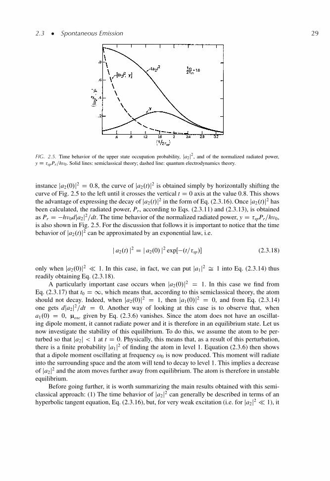
2.3 � Spontaneous Emission 29
FIG. 2.5. Time behavior of the upper state occupation probability, ja2j2, and of the normalized radiated power,y D �spPr=h�0. Solid lines: semiclassical theory; dashed line: quantum electrodynamics theory.
instance ja2.0/j2 D 0.8, the curve of ja2.t/j2 is obtained simply by horizontally shifting thecurve of Fig. 2.5 to the left until it crosses the vertical t D 0 axis at the value 0.8. This showsthe advantage of expressing the decay of ja2.t/j2 in the form of Eq. (2.3.16). Once ja2.t/j2 hasbeen calculated, the radiated power, Pr, according to Eqs. (2.3.11) and (2.3.13), is obtainedas Pr D �h�0dja2j2=dt. The time behavior of the normalized radiated power, y D �spPr=h�0,is also shown in Fig. 2.5. For the discussion that follows it is important to notice that the timebehavior of ja2.t/j2 can be approximated by an exponential law, i.e.
j a2.t/ j2 D j a2.0/ j2 expŒ�.t=�sp/� (2.3.18)
only when ja2.0/j2 � 1. In this case, in fact, we can put ja1j2 Š 1 into Eq. (2.3.14) thusreadily obtaining Eq. (2.3.18).
A particularly important case occurs when ja2.0/j2 D 1. In this case we find fromEq. (2.3.17) that t0 D 1, which means that, according to this semiclassical theory, the atomshould not decay. Indeed, when ja2.0/j2 D 1, then ja1.0/j2 D 0, and from Eq. (2.3.14)one gets dja2j2=dt D 0. Another way of looking at this case is to observe that, whena1.0/ D 0, μosc given by Eq. (2.3.6) vanishes. Since the atom does not have an oscillat-ing dipole moment, it cannot radiate power and it is therefore in an equilibrium state. Let usnow investigate the stability of this equilibrium. To do this, we assume the atom to be per-turbed so that ja2j < 1 at t D 0. Physically, this means that, as a result of this perturbation,there is a finite probability ja1j2 of finding the atom in level 1. Equation (2.3.6) then showsthat a dipole moment oscillating at frequency !0 is now produced. This moment will radiateinto the surrounding space and the atom will tend to decay to level 1. This implies a decreaseof ja2j2 and the atom moves further away from equilibrium. The atom is therefore in unstableequilibrium.
Before going further, it is worth summarizing the main results obtained with this semi-classical approach: (1) The time behavior of ja2j2 can generally be described in terms of anhyperbolic tangent equation, Eq. (2.3.16), but, for very weak excitation (i.e. for ja2j2 � 1), it
30 2 � Interaction of Radiation with Atoms and Ions
follows an approximately exponential law [Eq. (2.3.18)]. (2) When the atom is initially in theupper state (i.e. ja2.0/j2 D 1), the atom is in (unstable) equilibrium and no radiation occurs.
2.3.2. Quantum Electrodynamics Approach
Although a quantum electrodynamics approach is beyond the scope of this book, it isworthwhile to summarize some of the results obtained from such an approach and comparingthem with the semiclassical results. The most relevant results of the quantum approach canbe summarized as follows:.4,5/ (i) Unlike the semiclassical case, the time behavior of ja2j2 isnow always described, to a good approximation (Wigner-Weisskopf approximation), by anexponential law. This means that Eq. (2.3.18) is now always true, no matter what the value ofja2.0/j2. (ii) The expression of the spontaneous emission lifetime, �sp, turns out to be given, inthis case too, by Eq. (2.3.15). (iii) Since the radiated power is given by Pr D �h�0dja2j2=dt,this power will also decay exponentially with a time constant �sp. We see that the semiclas-sical and the quantum electrodynamics approaches give completely different predictions forthe phenomenon of spontaneous emission (see Fig. 2.5). All available experimental results�confirm that the quantum electrodynamics approach gives the correct answer to the problem.From Eq. (2.3.15) we can then write the rate of spontaneous emission, A D 1=�sp, as
A D 16 3�30 nj�j2
3h"0c30
(2.3.19)
The above remarks imply that, according to quantum electrodynamics, an atom in the upperlevel is not in a state of unstable equilibrium and the physical reason for the disappearance ofthis unstable state on passing from the semiclassical to the quantum electrodynamics approachdeserves some further discussion. In the semiclassical case, the atom’s wave function wasgenerally written as in Eq. (2.3.2) and this implies that the atom is not in a stationary state.According to quantum mechanics, this can only occur when some sort of perturbation isalready applied to the atom. Furthermore, to remove the unstable equilibrium position dis-cussed before, we need again to assume that the atom is somewhat perturbed, and we nowlook for some cause for this perturbation. At first sight we may be tempted to say that therewill always be enough stray radiation around the material to perturb the atom. To be morespecific, let us suppose that the material is contained in a blackbody cavity whose wallsare kept at temperature T. We might then imagine this stray radiation to be provided by theblackbody radiation within the cavity. This conclusion would be wrong, however, since theradiation produced in this way would actually be due to the process of stimulated emission,i.e., stimulated by the blackbody radiation. The phenomenon of spontaneous emission wouldthen depend upon the wall temperature and would cease at T D 0. The correct form of per-turbation needed to describe the phenomenon of spontaneous emission is actually providedby the quantum electrodynamics approach. In fact, according to the discussion presented in
� Of these, we should like to mention the very accurate measurements of the so-called Lamb shift, another phe-nomenon that occurs during spontaneous emission. The center frequency of the spontaneously emitted light doesnot occur at frequency �0 (the transition frequency) but at slightly different value. Lamb-shift measurements forhydrogen are among the most careful measurements so far made in physics, and they are always exactly agreed(within the experimental errors) with the predictions of the quantum electrodynamic approach.
2.3 � Spontaneous Emission 31
Sect. 2.2.3, the mean square values <E2> and <H2> of both the electric and magnetic fieldsof a given cavity mode are different from zero even at T D 0 (zero-point field fluctuations). Wemay therefore consider these fluctuations as the perturbation acting on the atom and which,in particular, upsets the unstable equilibrium predicted by the semiclassical treatment. Cor-respondingly we may think of the spontaneous emission process as originating from thesezero-point fluctuations.
2.3.3. Allowed and Forbidden Transitions
Equation (2.3.19) shows that, to have A ¤ 0, we must have j�j ¤ 0. In this case thespontaneous emission process arises from the power radiated by the electric dipole of theatom and the transition is said to be electric dipole allowed. By contrast, when j�j D 0, wehave A D 0 and the transition is said to be electric dipole forbidden. In this case the transitionmay occur via other multipole radiation processes e.g. through the oscillating magnetic dipolemoment of the atom (magnetic dipole transitions). This is usually a much weaker process,however.
Let us now consider the situation when the transition is electric dipole forbidden i.e.,when j�j D 0. Since j�j D jμ21j, Eq. (2.3.7) shows that this occurs when the eigenfunctionsu1 and u2 are either both symmetric or both anti symmetric�. In fact, in this case, the twocontributions from the integrand of Eq. (2.3.7) at points r and �r, respectively, are equal andopposite. It is therefore of interest to see when the wave functions u.r/ are either symmetricor anti symmetric. This occurs when the Hamiltonian Ho.r/ of the system is unchanged bychanging r into �r, i.e. when�
Ho.�r/ D Ho.r/ (2.3.20)
In this case, in fact, for any eigenfunction un.r/, one has
Ho.r/un.r/ D Enun.r/ (2.3.21)
From Eq. (2.3.21), changing r into �r and using Eq. (2.3.20), one gets
Ho.r/un.�r/ D Enun.�r/ (2.3.22)
Equations (2.3.21) and (2.3.22) show that un.r/ and un.�r/ are both eigenfunctions of theHamiltonian Ho with the same eigenvalue En. For non degenerate energy levels, there is, bydefinition only one eigenfunction for each eigenvalue, apart from an arbitrary choice of sign,so that
un.�r/ D ˙un.r/ (2.3.23)
Therefore, if Ho.r/ is symmetric, the eigenfunctions must be either symmetric or anti-symmetric. In this case, it is usually said that the eigenfunctions have a well definedparity.
� It may be recalled here that a function f .r/ is symmetric (or of even parity) if f .�r/ D f .r/, while it isantisymmetric (or of odd parity) if f .�r/ D �f .r/.
� If the Hamiltonian H0 is a function of more than one coordinate r1, r2, : : : . , the inversion operation must besimultaneously applied to all these coordinates.
32 2 � Interaction of Radiation with Atoms and Ions
Example 2.1. Estimate of �sp and A for electric-dipoleallowed and forbidden transitions For an electric-dipoleallowed transition at a frequency corresponding to themiddle of the visible range, an estimate the order ofmagnitude of A is obtained from Eq. (2.3.19) by theresubstituting the values � D c=� D 500 nm and j�j Šea, where a is the atomic radius .a Š 0.1 nm/. Wetherefore get A Š 108 s�1 (i.e. �sp Š 10 ns). For mag-netic dipole transitions A is approximately 105 timessmaller, and therefore �sp Š 1 ms. Note that, accordingto Eq. (2.3.19), A increases as the cube of the frequency,so that the importance of the process of spontaneousemission increases rapidly with frequency. In fact spon-taneous emission is often negligible in the middle to farinfrared where nonradiative decay usually dominates. Onthe other hand, when one considers the x-ray region (say� 5 nm), �sp becomes very short (10–100 fs) a fea-ture that constitutes a major problem for achieving apopulation inversion in X-ray lasers.
It remains now to see when the Hamil-tonian satisfies Eq. (2.3.20), i.e., when itis invariant under inversion. Obviously thisoccurs when the system has a center of sym-metry. Another important case is that of anisolated atom. In this case, the potentialenergy of the k-th electron of the atom isgiven by the sum of -the potential energy dueto the nucleus (which is symmetric) and thatof all other electrons. For the i-th electron,this energy will depend on jri�rkj, i.e., on themagnitude of the distance between the twoelectrons. Therefore, these terms will also beinvariant under inversion. An important casewhere Eq. (2.3.20) is not valid is where anatom is placed in an external electric field(e.g., a crystal’s electric field) that does notpossess a center of inversion. In this case thewave functions will not have a definite parity.
To sum up, we can say that electricdipole transitions only occur between states
of opposite parity, and that the states have a well-defined parity if the Hamiltonian is invariantunder inversion.
2.4. ABSORPTION AND STIMULATED EMISSION
In this section, we will study in some detail the processes of absorption and stimulatedemission induced in a two-level system for a single atom interacting with a monochromaticelectromagnetic (e.m.) wave. In particular, our aim is to calculate the rates of absorption W12
and stimulated emission W21 [see Eqs. (1.1.4) and (1.1.6)]. We will follow the semiclassicalapproximation, wherein, as already explained, the atom is quantized while the e.m. radiation istreated classically. It can be shown, in fact, that the quantum electrodynamics approach givesthe same result as the semiclassical treatment when the number of photons in a given radiationmode is much greater than unity. Since this applies to any system other than an exceedinglyweak e.m. wave, we can dispense with the complication of the full quantum treatment. Wewill at first assume the two levels to be non-degenerate and treat the case of degenerate levelslater in this Chapter.
2.4.1. Rates of Absorption and Stimulated Emission
Let us first consider the case of absorption and assume that, for time t 0, a monochro-matic e.m. wave is incident on the atom so that the atomic wave-function can be described asin Eq. (2.3.2) where we will assume the initial conditions ja1.0/j2 D 1 and ja2.0/j2 D 0.
2.4 � Absorption and Stimulated Emission 33
As a result of the interaction with the e.m. wave, the atom will acquire an interactionenergy H0. In the treatment that follows this energy H0 is considered to be due to the interac-tion of the electric dipole moment of the atom with the electric field E(r,t) of the e.m. wave(electric dipole interaction), where the origin of the r coordinate is taken at the nucleus. Theelectric field at the nuclear position can then be written as
E.0, t/ D E0sin.!t/ (2.4.1)
where ! is the angular frequency of the wave. We will also assume that the wavelength of thee.m. radiation is much greater than the atom’s dimension so that the phase-shift of the e.m.wave over an atomic dimension is very small. Then Eq. (2.4.1) can be taken to give the valueof the electric field for any location in the atom (electric dipole approximation). We will alsoassume the frequency ! to be close to the resonant frequency,!0, of the transition.
Classically, for a given position r of the electron within the atom, the atom would exhibitan electric dipole moment μ D �er, where e is the magnitude of the electronic charge. Theinteraction energy H0 resulting from the external electric field would then be
H0 D μ � E D �e � E0 sin!t (2.4.2)
In a quantum mechanical treatment, this sinusoidally time-varying interaction energy istreated as a sinusoidally time-varying interaction Hamiltonian H 0.t/, which is then insertedinto the time-dependent Schrodinger wave equation. Since ! Š !o, this interaction Hamil-tonian results in the transition of the atom from one level to the other. This implies that, fort > 0, ja1.t/j2 will decrease from its initial value ja1.0/j2 D 1 and ja2.t/j2 will increase cor-respondingly. To derive an expression for a2.t/ we will additionally assume that the transitionprobability is weak, so that a perturbation analysis can be used (time dependent perturbationtheory), and that the interaction occurs for a long time after t D 0.
Given the above assumptions, the time behaviour of ja2.t/j2 is shown, in Appendix A, tobe given by
ja2.t/j2 D 2
3h2j�21j2E2
0ı.� � �0/t (2.4.3)
where � D !=2 , �0 D !0=2 , ı is the Dirac delta function, E0 is the amplitude of the vectorE0 and jμ21j is the amplitude of the complex vector μ21 given by Eq. (2.3.7). Equation (2.4.3)shows that, for t > 0, ja2.t/j2 increases linearly with time. We can then define the transitionrate Wsa
12 as
Wsa12 D dja2j2=dt (2.4.4)
From Eq. (2.4.3) we then get
Wsa12 D 2
3h2j�21j2 E2
0ı.v � v0/ (2.4.5)
Note that the transition rate defined by Eq. (2.4.4) refers to the case of a single atom interactingwith monochromatic radiation and this situation is denoted by the superscript sa (single atom)added to W12.
34 2 � Interaction of Radiation with Atoms and Ions
To gain a more physical understanding of the absorption phenomenon, we begin by notic-ing that, for t > 0, the wave function can be described as in Eq. (2.3.2). For t > 0 the atomthus acquires an oscillating dipole moment, μosc, given by Eq. (2.3.6). In contrast to the caseof spontaneous emission, however, since a1.t/ and a2.t/ are now driven by the electric fieldof the e.m. wave, the phase of μosc turns out to be correlated to that of the wave. In particular,for absorption, i.e. when one starts with the initial conditions a1.0/ D 1 and a2.0/ D 0, thephase of the dipole is such that the dipole absorbs power from the e.m. wave. The interactionphenomenon is thus seen to be very similar to that of a classical oscillating dipole momentdriven by an external field..6/
Equation (2.4.5) can also be expressed in terms of the energy density of the e.m.wave. Since
� D n2"0E20=2 (2.4.6)
where n is the refractive index of the medium and "o is the vacuum permittivity, we obtain
Wsa12 D 2 2
3n2"0h2j�21j2�ı.� � �0/ (2.4.7)
Note that Wsa12 is proportional to the Dirac ı function. This implies the unphysical result that
W D 0 for � ¤ �0 and W12 D 1 when � D �0, i.e. when the frequency of the e.m. wave isexactly coincident with the frequency of the atomic transition. The reason for this unphysicalresult can be traced back to the assumption that the interaction of the e.m. wave with theatom could continue undisturbed for an indefinite time. Indeed, from a classical viewpoint,if a sinusoidal electric field at frequency � drives a (lossless) oscillating dipole moment atfrequency �0, there would only be an interaction, i.e. a net energy transfer, if � D �0. Actually,there are a number of perturbation phenomena (such as collisions with other atoms or withlattice phonons) that prevent this interaction from continuing undisturbed indefinitely. Thesephenomena will be discussed at some length in a later section, but the general result theylead to can be expressed in a very simple way: Eq. (2.4.7) remains valid provided the Diracı function – an infinitely sharp function centred at � D �0 and of unit area, i.e., such thatRı.� � �0/d� D 1 – be replaced by a new function g.� � �0/, symmetric about � D �0 again
of unit area, i.e. such thatR
g.� � �0/d� D 1, and generally given by
g.� � �0/ D 2
�0
1
1 C Œ2.� � �0/=�0�2(2.4.8)
where�o depends on the particular broadening mechanism involved. We can therefore writefor Wsa
12 the expression
Wsa12 D 2 2
3n2"0h2j�21j2�g.� � �0/ (2.4.9)
The normalized function Œg.� � �0/�0� is plotted in Fig. 2.6 vs the normalized frequencydifference .� � �0/=.�0=2/. The full width of the curve between the two points having
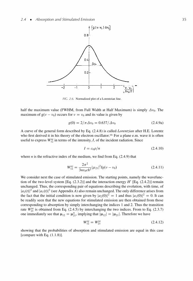
2.4 � Absorption and Stimulated Emission 35
FIG. 2.6. Normalized plot of a Lorentzian line.
half the maximum value (FWHM, from Full Width at Half Maximum) is simply �0. Themaximum of g.� � �0/ occurs for � D �0 and its value is given by
g.0/ D 2= �0 D 0.637=�0 (2.4.9a)
A curve of the general form described by Eq. (2.4.8) is called Lorentzian after H.E. Lorentzwho first derived it in his theory of the electron oscillator..6/ For a plane e.m. wave it is oftenuseful to express Wsa
12 in terms of the intensity, I, of the incident radiation. Since
I D c0�=n (2.4.10)
where n is the refractive index of the medium, we find from Eq. (2.4.9) that
Wso12 D 2 2
3n"0ch2j�21j2Ig.� � �0/ (2.4.11)
We consider next the case of stimulated emission. The starting points, namely the wavefunc-tion of the two-level system [Eq. (2.3.2)] and the interaction energy H0 [Eq. (2.4.2)] remainunchanged. Thus, the corresponding pair of equations describing the evolution, with time, ofja2.t/j2 and ja1.t/j2 (see Appendix A) also remain unchanged. The only difference arises fromthe fact that the initial condition is now given by ja2.0/j2 D 1 and thus ja1.0/j2 D 0. It canbe readily seen that the new equations for stimulated emission are then obtained from thosecorresponding to absorption by simply interchanging the indices 1 and 2. Thus the transitionrate Wsa
21 is obtained from Eq. (2.4.5) by interchanging the two indices. From to Eq. (2.3.7)one immediately see that μ12 D μ�
21, implying that jμ12j D jμ21j. Therefore we have
Wsa12 D Wsa
21 (2.4.12)
showing that the probabilities of absorption and stimulated emission are equal in this case[compare with Eq. (1.1.8)].
36 2 � Interaction of Radiation with Atoms and Ions
As a conclusion to this section, according to Eqs. (2.4.9) and (2.4.11), the stimulatedtransition rate can be written as�
Wsa D 2 2
3n2"0h2j�j2�g.� � �0/. (2.4.13)
Wsa D 2 2
3n"0ch2j�j2Ig.� � �0/ (2.4.13a)
where, from Eq. (2.4.12), we have set Wsa D Wsa12 D Wsa
21. and where we have also setj�j D jμ12j D jμ21j.
2.4.2. Allowed and Forbidden Transitions
Equations (2.4.13) and (2.3.19) show that the transition rate Wsa, and the spontaneousemission rate A are proportional to j�j2. This indicates that the two phenomena must obeythe same selection rule. Thus the stimulated transition via electric dipole interaction (electricdipole transition) only occurs between states, u1 and u2, of opposite parity. The transitionis then said to be electric dipole allowed. Conversely, if the parity of the two states is thesame, then Wsa D 0 and the transition is said to be electric-dipole forbidden. This doesnot mean, however, that the atom cannot pass from level 1 to level 2 through the influenceof an incident e.m. wave. In this case, the transition can occur, for instance, as a result ofthe interaction of the magnetic field of the e.m. wave with the magnetic dipole moment ofthe atom. For the sake of simplicity, we will not consider this case any further (magneticdipole interaction), but limit ourselves to observing that the analysis can be carried out in asimilar manner to that used to obtain Eq. (2.4.11). We may also point out that a magneticdipole transition is allowed between states of equal parity (even-even or odd-odd transitions).Therefore, a transition that is forbidden by electric dipole interaction is, however, allowedfor magnetic dipole interaction and vice versa. It is also instructive to calculate the orderof magnitude of the ratio of the electric dipole transition probability, We, to the magneticdipole transition probability, Wm. Obviously the calculation refers to two different transitions,one being allowed for electric dipole and the other for magnetic dipole interaction. We shallassume that the intensity of the e.m. wave is the same for the two cases. For an allowedelectric dipole transition, according to Eq. (2.4.5), we can write We / .�eE0/
2 � .eaE0/2,
where E0 is the electric field amplitude and where the electric dipole moment of the atom�e has been approximated (for an allowed transition) by the product of the electron charge
� It should be noted that the factor 3 appearing in the denominator of Eq. (2.4.3) and, hence, of Eq. (2.4.5),Eq. (2.4.7), Eq. (2.4.9), Eq. (2.4.11), Eqs. (2.4.13), and (2.4.13a), refers to the case of a linearly polarized waveinteracting with randomly oriented atoms (such as in a gas). In this case, in fact, we have W /< jμ21 � E0j2 >Dj�21j2 D j�21j2E2
0<cos2 > D j�21j2 E20=3, where is the angle between μ21 and E0 and the average is taken
over all atom-field orientations. Indeed, for randomly oriented μ21 vectors, one has < cos2 > D 1=3 where theaverage is taken in the three dimensional space, i.e.< cos2 > D R
cos2 d˝=4 . For different cases of atom/fieldorientation, the factor j�21j2 =3 should be changed appropriately. Thus, for aligned ions (such as in ionic crystals)and a linearly polarized wave, the factor 3 should be dropped and j�21j should represent the magnitude of thecomponent of μ21 along E0.
2.4 � Absorption and Stimulated Emission 37
e and the radius a of the atom. For a magnetic dipole interaction, it can likewise be shownthat Wm / .�mB0/
2 � .ˇB0/2, where B0 is the magnetic field amplitude of the wave and
where the magnetic dipole moment of the atom, �m, has been approximated (for an allowedtransition) by the Bohr magneton ˇ .ˇ D 9.27 � 10�24 A � m2/. Thus we get
.We=Wm/ D .eaE0=ˇB0/2 D .eac=ˇ/2 Š 105 (2.4.14)
To obtain the numerical result of Eq. (2.4.14) we have made use of the fact that, for a planewave it is E0=B0 D c (where c is the light velocity), and we have assumed that a Š 0.5 nm.The probability of an electric dipole transition is thus much greater than that of a magneticdipole.
2.4.3. Transition Cross Section, Absorption and Gain Coefficient
In Sect. 2.4.1, the transition rate has been calculated for the case of a single atom interact-ing with an incident e.m. wave and whose linewidth is determined by some line-broadeningmechanism. We now consider an ensemble of Nt atoms per unit volume and we want tocalculate the corresponding, average, transition rate.
The first case we will consider is where both the resonance frequency �0 and the lineshape are the same for every atom (the case of homogeneous broadening). The transition rate,Wh, for this homogeneous case will then be the same for every atom, so that we can simplywrite
Wh.� � �0/ D Wsa.� � �0/ (2.4.15)
If we now let all atoms be in the ground state, the power absorbed per unit volume, dPa=dV,will then be given by
.dPa=dV/ D WhNth� (2.4.16)
Since Wh is proportional to the wave intensity, hence to the photon flux F D I=h�, we candefine an absorption cross section, �h, as
�h D Wh=F (2.4.17)
From Eqs. (2.4.13a) and (2.4.17), �h is seen to be given by
�h D 2 2
3n"0chj�j2�g.� � �0/ (2.4.18)
With the help of the same argument used in connection with Fig. 1.2, we obtain fromEqs. (2.4.16) and (2.4.17) the equation describing the variation of the photon flux along the zdirection as [compare with Eq. (1.2.1)]
dF D �� NtFdz (2.4.19)
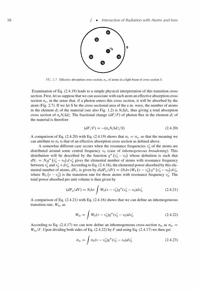
38 2 � Interaction of Radiation with Atoms and Ions
FIG. 2.7. Effective absorption cross section, �a , of atoms in a light beam of cross section S.
Examination of Eq. (2.4.19) leads to a simple physical interpretation of this transition crosssection. First, let us suppose that we can associate with each atom an effective absorption crosssection �a, in the sense that, if a photon enters this cross section, it will be absorbed by theatom (Fig. 2.7). If we let S be the cross-sectional area of the e.m. wave, the number of atomsin the element dz of the material (see also Fig. 1.2) is NtSdz, thus giving a total absorptioncross section of �aNtSdz. The fractional change .dF=F/ of photon flux in the element dz ofthe material is therefore
.dF=F/ D �.�aNtSd z=S/ (2.4.20)
A comparison of Eq. (2.4.20) with Eq. (2.4.19) shows that �h D �a, so that the meaning wecan attribute to �h is that of an effective absorption cross section as defined above.
A somewhat different case occurs when the resonance frequencies �00 of the atoms are
distributed around some central frequency �0 (case of inhomogeneous broadening). Thisdistribution will be described by the function g� �0
0 � �0�
whose definition is such thatdNt D Ntg� �0
0 � �0�
d �00 gives the elemental number of atoms with resonance frequency
between � 00 and �0
0 Cd� 00. According to Eq. (2.4.16), the elemental power absorbed by this ele-
mental number of atoms, dNt, is given by d.dPa=dV/ D .Nth�/Wh� � �0
0
�g� �0
0 � �0�
d�00,
where Wh� � �0
0
�is the transition rate for those atoms with resonance frequency �0
0. Thetotal power absorbed per unit volume is then given by
.dPa=dV/ D Nth�Z
Wh.� � � 00/g
�.�00 � �0/d�
00 (2.4.21)
A comparison of Eq. (2.4.21) with Eq. (2.4.16) shows that we can define an inhomogeneoustransition rate, Win, as
Win DZ
Wh.� � �00/g
�.�00 � �0/d�
00 (2.4.22)
According to Eq. (2.4.17) we can now define an inhomogeneous cross-section �in as �in DWin=F. Upon dividing both sides of Eq. (2.4.22) by F and using Eq. (2.4.17) we then get
�in DZ�h.� � � 0
0/g�.�0
0 � �0/d�00 (2.4.23)
2.4 � Absorption and Stimulated Emission 39
Following the argument presented in connection with Fig. 2.7 one can see that �in is an effec-tive absorption cross section that one can associate with a single atom, so that a photon willbe absorbed if it enters this cross section. Note, however, that, in this case each atom has,in reality, a different cross section �h.� � �0
0/ at the frequency of the incoming radiation and�in is just an effective average cross section. Note also that, according to Eq. (2.4.23), theline shape and linewidth of �in depend on the function g� �0
0 � �0�
i.e. on the distribution ofthe atomic resonance frequencies. The phenomena leading to this frequency distribution willbe discussed at some length in a later section. Here we limit ourselves to pointing out thatg� �0
0 � �0�
is generally described by a function of the form
g�.�00 � �0/ D 2
��0
�ln 2
�1=2
exp ��
4.�00 � �0/
2
��20
ln 2
�(2.4.24)
where ��o is the transition linewidth (FWHM), its value depending of the particular
broadening mechanism under consideration.With the help of Eq. (2.4.18), Eq. (2.4.23) can be transformed to
�in D 2 2
3n"0chj�j2�gt.� � �0/ (2.4.25)
In Eq. (2.4.25) we have used the symbol gt.�� �0/ for the total line shape function which canbe expressed as
gt DZ C1
�1g�.x/g Œ.� � �0/ � x� dx (2.4.26)
where we have put x D � 00 ��0. The expression of the cross section for inhomogeneous broad-
ening, �in, is thus obtained from that for homogeneous broadening, given by Eq. (2.4.18), bysubstituting g.� � �0/ with gt.� � �0/. Note that, according to Eq. (2.4.26), gt is the convolu-tion of the functions g and g�. Since both functions are normalised to unity it can be shownthat gt is also normalised to unity, i.e. that
Rgt.� � �o/d� D 1. Note also that Eq. (2.4.25)
provides a generalisation of Eq. (2.4.18). Indeed, it is immediately seen from Eqs. (2.4.26)and (2.4.25) that �in reduces to �h when g� �0
0 � �0� D ı
� 0
0 � �0�, i.e. when all atoms have
the same resonance frequency. Conversely, if the width of the line shape function, g� � �0
0
�,
is much smaller than that due to inhomogeneous broadening, g� �00 � �0
�, then g
� � �0
0
�can be approximated by a Dirac ı function in Eq. (2.4.26) and one gets gt Š g�.� � �0/ (caseof pure inhomogeneous broadening). In this case from Eq. (2.4.24) we get
gt D g�.� � �0/ D 2
��0
�ln 2
�1=2
exp ��
4.� � �0/2
��0
ln 2
�(2.4.27)
The normalized function�g�.� � �0/�
�0
is plotted in Fig. 2.8 vs the normalized frequency
difference .� � �0/=��
0 =2�. According to Eq. (2.4.27), the width of the curve (FWHM) is
simply ��0 , the maximum of the function occurs for � D �0 and its value is given by
g�.0/ D 2
��0
�ln 2
�1=2
D 0.939
��0
(2.4.28)
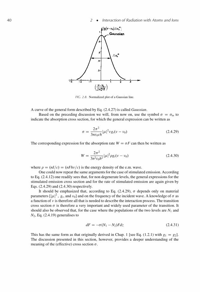
40 2 � Interaction of Radiation with Atoms and Ions
FIG. 2.8. Normalized plot of a Gaussian line.
A curve of the general form described by Eq. (2.4.27) is called Gaussian.Based on the preceding discussion we will, from now on, use the symbol � D �in to
indicate the absorption cross section, for which the general expression can be written as
� D 2 2
3n"0chj�j2�gt.� � �0/ (2.4.29)
The corresponding expression for the absorption rate W D �F can then be written as
W D 2 2
3n2"0h2j�j2�gt.� � �0/ (2.4.30)
where � D .nI=c/ D .nFh�=c/ is the energy density of the e.m. wave.One could now repeat the same arguments for the case of stimulated emission. According
to Eq. (2.4.12) one readily sees that, for non degenerate levels, the general expressions for thestimulated emission cross section and for the rate of stimulated emission are again given byEqs. (2.4.29) and (2.4.30) respectively.
It should be emphasized that, according to Eq. (2.4.29), � depends only on materialparameters [j�j2 , gt, and �0] and on the frequency of the incident wave. A knowledge of � asa function of � is therefore all that is needed to describe the interaction process. The transitioncross section � is therefore a very important and widely used parameter of the transition. Itshould also be observed that, for the case where the populations of the two levels are N1 andN2, Eq. (2.4.19) generalises to
dF D ��.N1 � N2/Fdz (2.4.31)
This has the same form as that originally derived in Chap. 1 [see Eq. (1.2.1) with g1 D g2].The discussion presented in this section, however, provides a deeper understanding of themeaning of the (effective) cross section � .
2.4 � Absorption and Stimulated Emission 41
Another way of describing the interaction of radiation with matter involves defining aquantity ˛ as
˛ D �.N1 � N2/ (2.4.32)
If N1 > N2 then ˛ is positive and is referred to as the absorption coefficient of the material.Using Eq. (2.4.29) the following expression is obtained for ˛:
˛ D 2 2
3n"0ch.N1 � N2/j�j2�gt.� � �0/ (2.4.33)
Since ˛ depends on the populations of the two levels, it is not the most suitable parameterfor describing a situation where the level populations are changing, such as, for example, ina laser. Its usefulness, however, lies in the fact that the absorption coefficient ˛ can often bedirectly measured. From Eqs. (2.4.31) and (2.4.32) we get in fact
dF D �˛Fdz (2.4.34)
The ratio between the photon flux after traversing a length l of the material and the incidentflux is therefore ŒF.l/=F.0/� D exp.�˛l/. By experimentally measuring this ratio with a suffi-ciently monochromatic radiation, we can obtain the value of ˛ for that particular wavelength.The corresponding value of the transition cross section is then obtained from Eq. (2.4.32)once N1 and N2 are known. If the medium is in thermodynamic equilibrium, N1 and N2 can beobtained from Eq. (1.2.2) once the total population Nt D N1 C N2 and the level’s degenera-cies are known. The instrument used the measure the absorption coefficient ˛ is known as anabsorption spectrophotometer. We note, however, that an absorption measurement obviouslycannot be performed for a transition in which level 1 is empty. This situation, for instance,occurs when level 1 is not the ground level and its energy above the ground level is muchlarger than kT. As a final observation we note that if N2 > N1, the absorption coefficient ˛,defined by Eq. (2.4.32), becomes negative and, of course, the wave gets amplified rather thanabsorbed in the material. In this case it is customary to define the new quantity g, as
g D �.N2 � N1/ (2.4.35)
which is positive and is called the gain coefficient.
2.4.4. Einstein Thermodynamic Treatment
In this section we will describe a treatment, given by Einstein,.7/ of both spontaneous andstimulated transitions (absorption and emission). In this treatment the concept of stimulatedemission was first clearly established and the correct relationship between spontaneous andstimulated transition rates was derived well before the formulation of quantum mechanics andquantum electrodynamics. The calculation makes use of an elegant thermodynamic argument.To this end, let us assume that the material is placed in a blackbody cavity whose wallsare kept at a constant temperature T. Once thermodynamic equilibrium is reached, an e.m.energy density with a spectral distribution �� given by Eq. (2.2.22) will be established and
42 2 � Interaction of Radiation with Atoms and Ions
the material will be immersed in this radiation. In this material, both stimulated-emission andabsorption processes will occur, in addition to the spontaneous-emission process. Since thesystem is in thermodynamic equilibrium, the number of transitions per second from level 1 tolevel 2 must be equal to the number of transitions from level 2 to level 1. We now set
W21 D B21��0 (2.4.36)
W12 D B12��0 (2.4.37)
where B21 and B12 are constant coefficients (the Einstein B coefficients), and let Ne1 and Ne
2 bethe equilibrium populations of levels 1 and 2, respectively. We can then write
ANe2 C B21�v0 Ne
2 D B12�v0 Ne1 (2.4.38)
From Boltzmann statistics we also know that, for non degenerate levels, one has
Ne2=Ne
1 D exp.�h�0=kT/ (2.4.39)
From Eqs. (2.4.38) and (2.4.39) it then follows that
��0 D A
B12 exp.h�0=kT/ � B21(2.4.40)
A comparison of Eq. (2.4.40) with Eq. (2.2.22), when � D �0, leads to the following relations:
B12 D B21 D B (2.4.41)
A
BD 8 h�3
0n3
c3(2.4.42)
Equation (2.4.41) shows that the probabilities of absorption and stimulated emission due toblackbody radiation are equal. This relation is therefore analogous to that established, in acompletely different way, in the case of monochromatic radiation [see Eq. (2.4.12)]. Equa-tion (2.4.42), on the other hand, allows the calculation of A, once B, i.e., the coefficientfor stimulated emission due to blackbody radiation, is known. This coefficient can easilybe obtained from Eq. (2.4.30) once we remember that this equation was established formonochromatic radiation. For blackbody radiation, we can write ��d� for the energy den-sity of radiation whose frequency lies between � and � C d� and simulate this elementalradiation by a monochromatic wave. The corresponding elemental transition probability dWis then obtained from Eq. (2.4.30) by substituting ��d� for �. Upon integration of the resultingequation with the assumption that gt.� � �0/ can be approximated by a Dirac ı function incomparison with �� (see Fig. 2.3), we get
W D 2 2
3 n2"0 h2j�j2��0 (2.4.43)
The comparison of Eq. (2.4.43) with Eqs. (2.4.36) or (2.4.37) then gives
B D 2 2j�j23 n2"0 h2
(2.4.44)
2.5 � Line Broadening Mechanisms 43
so that, from Eq. (2.4.42), we obtain
A D 16 3�30 nj�j2
3 h"0 c3(2.4.45)
It should be noted that the expression for A that we have just obtained is exactly the sameas that obtained by a quantum electrodynamics approach [see Eq. (2.3.19)]. Its calcula-tion is in fact based on thermodynamics and the use of Planck’s law (which is quantumelectrodynamically correct).
2.5. LINE BROADENING MECHANISMS
In this section we will discuss, in some detail, the various line broadening mechanismsmentioned in previous sections. According to the earlier discussion, there is an importantdistinction to be made from the outset between homogeneous and inhomogeneous line-broadening. A line-broadening mechanism is referred to as homogeneous when it broadensthe line of each atom in the same way. In this case the line-shape of the single-atom crosssection and that of the overall absorption cross section would be identical. Conversely, a line-broadening mechanism is said to be inhomogeneous when it distributes the atomic resonancefrequencies over some spectral range. Such a mechanism thus broadens the overall line of thesystem (i.e. that of ˛) without broadening the lines of individual atoms.
Before proceeding, it is worth recalling that the shape of the function gt.� � �0/ canbe determined in two ways: (a) By an absorption experiment, with the help of a spectropho-tometer. In this case one measures the absorption coefficient as a function of frequency �,using the spectrophotometer to select the light frequency. From Eq. (2.4.33) one sees that˛ / �gt.� � �0/. Since the linewidth of the function gt.� � �0/ is, typically, much smallerthan �0, we can approximately write ˛ / �0gt.� � �0/. Thus, to a very good approximation,the shape of the ˛ vs � curve coincides with that of the function gt.� � �0/. (b) By an emis-sion experiment, in which one passes the spontaneously emitted light trough a spectrometerof sufficiently high resolution and one determines gt.� � �0/ by measuring the shape of thespectral emission. It can be shown that, for any transition, the lineshapes obtained by thesetwo approaches are always the same. So, in the discussion that follows, we will consider thelineshape function either in absorption or in emission, whichever is the more convenient.
2.5.1. Homogeneous Broadening
The first homogeneous line-broadening mechanism we consider is one due to collisionsand is known as collision broadening. In a gas, it is due to the collision of an atom withother atoms, ions, free electrons, etc. or with the walls of the container. In a solid it is dueto the interaction of the atom with the phonons of the lattice. After a collision the two levelwavefunctions 1 and 2 of the atom [see Eq. (2.3.1)] will undergo a random phase jump.This means that the phase of the oscillating dipole moment μosc [see Eq. (2.3.6)] will undergoa random jump compared to that of the incident e.m. wave. These collisions thus interrupt
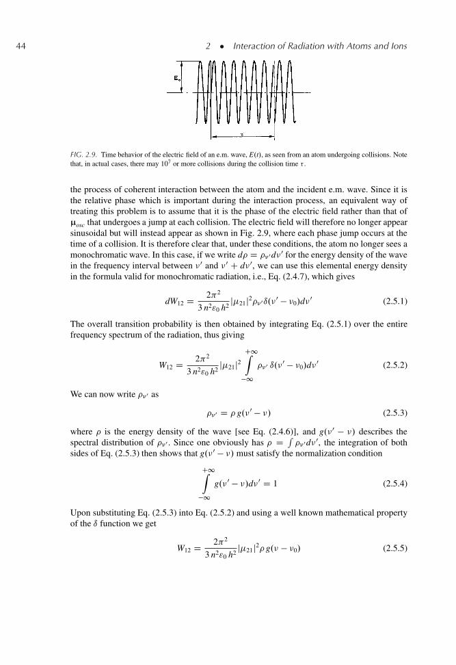
44 2 � Interaction of Radiation with Atoms and Ions
FIG. 2.9. Time behavior of the electric field of an e.m. wave, E.t/, as seen from an atom undergoing collisions. Notethat, in actual cases, there may 107 or more collisions during the collision time � .
the process of coherent interaction between the atom and the incident e.m. wave. Since it isthe relative phase which is important during the interaction process, an equivalent way oftreating this problem is to assume that it is the phase of the electric field rather than that ofμosc that undergoes a jump at each collision. The electric field will therefore no longer appearsinusoidal but will instead appear as shown in Fig. 2.9, where each phase jump occurs at thetime of a collision. It is therefore clear that, under these conditions, the atom no longer sees amonochromatic wave. In this case, if we write d� D ��0d�0 for the energy density of the wavein the frequency interval between �0 and �0 C d�0, we can use this elemental energy densityin the formula valid for monochromatic radiation, i.e., Eq. (2.4.7), which gives
dW12 D 2 2
3 n2"0 h2j�21j2��0ı.�0 � �0/d�
0 (2.5.1)
The overall transition probability is then obtained by integrating Eq. (2.5.1) over the entirefrequency spectrum of the radiation, thus giving
W12 D 2 2
3 n2"0 h2j�21j2
C1Z�1
��0 ı.�0 � �0/d�0 (2.5.2)
We can now write ��0 as
��0 D � g.�0 � �/ (2.5.3)
where � is the energy density of the wave [see Eq. (2.4.6)], and g.�0 � �/ describes thespectral distribution of ��0 . Since one obviously has � D R
��0d�0, the integration of bothsides of Eq. (2.5.3) then shows that g.�0 � �/ must satisfy the normalization condition
C1Z�1
g.�0 � �/d�0 D 1 (2.5.4)
Upon substituting Eq. (2.5.3) into Eq. (2.5.2) and using a well known mathematical propertyof the ı function we get
W12 D 2 2
3 n2"0 h2j�21j2� g.� � �0/ (2.5.5)
2.5 � Line Broadening Mechanisms 45
As anticipated in Sect. 2.4.1, it is seen that W12 is indeed obtained by substituting g.� � �0/
to ı.� � �0/ in Eq. (2.4.7). Note that, according to Eq. (2.5.4), we also have
C1Z�1
g.� � �0/d� D 1 (2.5.6)
There now remains the problem of calculating the normalized spectral density of the incidentradiation g.�0 � �/. This will depend on the time interval, � , between collisions (Fig. 2.9),which will obviously be different for each collision. We will assume that the distribution ofthe values of � can be described by a probability density
p� D Œexp.��=�c/�=�c (2.5.7)
Here p� d� is the probability that the time interval between two successive collisions liesbetween � and �Cd� . Note that �c has the physical meaning of the average time<�> betweencollisions. It is easy, in fact, to see that
<�> D1Z
0
� p� d� D �c (2.5.8)
At this point the mathematical problem to be solved is well defined. We need to obtain thenormalized spectral lineshape of a wave as in Fig. 2.9 for which the time � between twosuccessive collisions has the statistical distribution p� given by Eq. (2.5.7). Referring to theAppendix B for the mathematical details we merely quote the final result here. The requirednormalized spectral lineshape is given by
g.�0 � �/ D 2�c1�
1 C 4 2�2c .�
0 � �/2 (2.5.9)
According to Eq. (2.5.5) the line shape of the transition is obtained from Eq. (2.5.9) bysubstituting �0 by �0. We then get
g.� � �0/ D 2�c1�
1 C 4 2�2c .� � �0/2
(2.5.10)
which is our final result. We thus obtain a function with a Lorentzian lineshape, as generallydescribed by Eq. (2.4.8) [see also Fig. 2.6], where the peak value is now 2�c and the linewidth�0 is
�0 D 1= �c (2.5.11)
Example 2.2. Collision broadening of a He-Ne laser As a first example of collision broadening, weconsider the case of a transition for an atom, or ion, in a gas at pressure p. An estimate of �c is, in thiscase, given by �c D l=�th where l is the mean free path of the atom in the gas and �th is its average thermalvelocity. Since �th D .3kT=M/1=2 where M is the atomic mass and taking l to be given by the expressionresulting from the hard-sphere model of a gas, we obtain
46 2 � Interaction of Radiation with Atoms and Ions
�c D�
2
3
�1=2 1
8
.MkT/1=2
pa2(2.5.12)
where a is the radius of the atom and p is the gas pressure. For a gas of Neon atoms at room temper-ature and at a pressure p Š 0.5 Torr (typical pressure in a He-Ne gas laser) using Eq. (2.5.12) witha Š 0.1 nm and �c Š 0.5�s, we find from Eq. (2.5.11) that �o D 0.64 MHz. Note that �c is inverselyproportional, and hence �0 directly proportional, to p. As a rough “rule of thumb” we can say that, forany atom, collisions in a gas contribute to the line broadening by an amount .�0=p/ Š 1 MHz=Torr, com-parable to that shown in the example of Ne atoms. Note also that, during the collision time �c the numberof cycles of the e.m. wave is equal to m D ��c For a wave whose wavelength falls in the middle of the vis-ible range we have � D 5�1014 Hz and thus the number of cycles is 5�108. This emphasizes the fact thatFig. 2.9 is not to scale since the number of cycles in the time � is much larger than suggested in the figure.
Example 2.3. Linewidth of Ruby and Nd:YAG As a third example of collision broadening, we will con-sider an impurity ion in an ionic crystal. In this case the collisions of the ion occur with the latticephonons. Since the number of phonons in a given lattice vibration is a strong function of the latticetemperature, we expect the transition linewidth to show a strong dependence on temperature. As a rep-resentative example, Fig. 2.10 shows the linewidth versus temperature for both Nd:YAG and ruby, thelinewidth being expressed in wavenumbers Œcm�1�, a quantity widely used by spectroscopists rather thanactual frequency.� At 300 K the laser transition linewidths are seen to be �0 Š 4 cm�1 Š 120 GHz forNd:YAG and �0 Š 11 cm�1 D 330 GHz for ruby.
A second homogeneous line-broadening mechanism has its origin in the phenomenon ofspontaneous emission. Since this emission is an inevitable feature of any transition, the cor-responding broadening is called natural or intrinsic. In the case of natural broadening, it iseasiest to consider the behavior in terms of the spectrum of the emitted radiation. It should benoted however that, as pointed out in Sect. 2.3.2, spontaneous emission is a purely quantumphenomenon, i.e. it can only be correctly explained by quantizing both matter and radia-tion. It follows therefore that a correct description of the lineshape of the emitted radiationalso needs a quantum electrodynamics treatment. We will therefore limit ourselves to quot-ing the final result, which happens to be very simple, and to justifying it by some simplearguments. The quantum electrodynamics theory of spontaneous emission.8/ shows that thespectrum g.� � �0/ is again described by a Lorentzian line whose shape can be obtained fromEq. (2.5.10) by replacing �c by 2�sp, where �sp is the decay time of the spontaneous emission.Thus, in particular, the full width of the line (FWHM) is given by
�0 D 1=2 �sp (2.5.13)
� For a given wave of frequency v, the corresponding frequency in wave numbers (e.g. in cm�1) is given by w D1=C, where c is the velocity of the wave in a vacuum (in cm/s). The true frequency v is then obtained from thefrequency in wave numbers by the simple relation v D cw while the corresponding wavelenght is simply givenby � D c=v D 1=w (in cm). This illustrates the advantages of the wave number notation. The trem wave numberarises from the fact that w gives the number of wave periods, n, comprised in a given unitary length l (e.g. in 1cm). The number n is in fact given by n D l=� so that n=l D 1� D w.
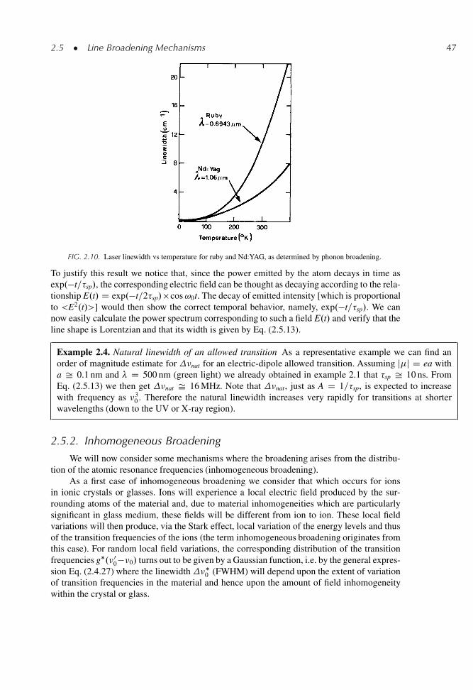
2.5 � Line Broadening Mechanisms 47
FIG. 2.10. Laser linewidth vs temperature for ruby and Nd:YAG, as determined by phonon broadening.
To justify this result we notice that, since the power emitted by the atom decays in time asexp.�t=�sp/, the corresponding electric field can be thought as decaying according to the rela-tionship E.t/ D exp.�t=2�sp/�cos!0t. The decay of emitted intensity [which is proportionalto <E2.t/>] would then show the correct temporal behavior, namely, exp.�t=�sp/. We cannow easily calculate the power spectrum corresponding to such a field E.t/ and verify that theline shape is Lorentzian and that its width is given by Eq. (2.5.13).
Example 2.4. Natural linewidth of an allowed transition As a representative example we can find anorder of magnitude estimate for �nat for an electric-dipole allowed transition. Assuming j�j D ea witha Š 0.1 nm and � D 500 nm (green light) we already obtained in example 2.1 that �sp Š 10 ns. FromEq. (2.5.13) we then get �nat Š 16 MHz. Note that �nat, just as A D 1=�sp, is expected to increasewith frequency as �3
0 . Therefore the natural linewidth increases very rapidly for transitions at shorterwavelengths (down to the UV or X-ray region).
2.5.2. Inhomogeneous Broadening
We will now consider some mechanisms where the broadening arises from the distribu-tion of the atomic resonance frequencies (inhomogeneous broadening).
As a first case of inhomogeneous broadening we consider that which occurs for ionsin ionic crystals or glasses. Ions will experience a local electric field produced by the sur-rounding atoms of the material and, due to material inhomogeneities which are particularlysignificant in glass medium, these fields will be different from ion to ion. These local fieldvariations will then produce, via the Stark effect, local variation of the energy levels and thusof the transition frequencies of the ions (the term inhomogeneous broadening originates fromthis case). For random local field variations, the corresponding distribution of the transitionfrequencies g�.�0
0��0/ turns out to be given by a Gaussian function, i.e. by the general expres-sion Eq. (2.4.27) where the linewidth ��
0 (FWHM) will depend upon the extent of variationof transition frequencies in the material and hence upon the amount of field inhomogeneitywithin the crystal or glass.
48 2 � Interaction of Radiation with Atoms and Ions
Example 2.5. Linewidth of a Nd:glass laser As a rep-resentative example we consider the case of Nd3C ionsdoped into a silicate glass. In this case, due to glassinhomogeneities, the linewidth of the laser transition at� D 1.05�m is ��
0 Š 5.4 THz i.e. it is about 40times broader than that of Nd:YAG at room temperature(see Example 2.3). It should be noted that these inhomo-geneities are an unavoidable feature of the glass state.
A second inhomogeneous broadeningmechanism, typical of gas, arises fromatomic motion and is called Doppler broad-ening. Assume that an incident e.m. waveof frequency � is propagating in the positivez direction and let �z be the component ofatomic velocity along this axis. According tothe Doppler effect, the frequency of the wave,as seen from the rest frame of the atom, is�0 D �Œ1 � .�z=c/� where c is the velocity of
light in the medium. Notice the well known result that, when �z > 0, we have �0 < � andvice versa. Of course, absorption by the atom will occur only when the apparent frequency �0of the e.m. wave, as seen from the atom, is equal to the atomic transition frequency �0, i.e.,when �Œ1 � .�z=c/� D �0. If we now express this relation as
� D �0=Œ1 � .�z=c/� (2.5.14)
we can arrive at a different interpretation of the process. As far as the interaction of the e.m.radiation with the atom is concerned, the result would be the same if the atom were not movingbut instead had a resonant frequency �0
0 given by
�00 D �0=Œ1 � .�z=c/� (2.5.15)
where �0 is the true transition frequency. Indeed, following this interpretation, absorptionis expected to occur when the frequency � of the e.m. wave is equal to �0
0 i.e. when � D�0
0, in agreement with Eq. (2.5.14) when the expression Eq. (2.5.15) for �00 is used. When
looked at in this way, one can see that this broadening mechanism does indeed belong to theinhomogeneous category as defined at the beginning of this section.
To calculate the corresponding line shape g�.�00 � �0/ it is now sufficient to remember
that, if we let pvd�z be the probability that an atom of mass M in a gas at temperature T has avelocity component between �z and �z C d�z, then pv is given by the Maxwell distribution
p� D�
M
2 kT
�1=2
exp �.M�2z =2kT/ (2.5.16)
From Eq. (2.5.15), since j�zj � c, we get �00 Š �0Œ1 C .�z=c/� and thus �z D c.�0
0 � �0/=�0.From Eq. (2.5.16) one then obtains the desired distribution upon recognizing that one musthave g�.�0
0 � �0/d� 00 D p�d�z. One then gets
g�.�00 � �0/ D 1
�0
�Mc2
2 kT
�1=2
exp �"
Mc2
2kT
� 0
0 � �0�2
�20
#(2.5.17)
Thus one again obtains a Gaussian function whose FWHM linewidth (Doppler linewidth) isnow readily found from a comparison of Eq. (2.5.17) with Eq. (2.4.24), giving
��0 D 2�0
�2kT ln 2=Mc21=2
(2.5.18)
For the purely inhomogeneous case the lineshape will be given by the general expression ofEq. (2.4.27) where��
0 is given by Eq. (2.5.18).
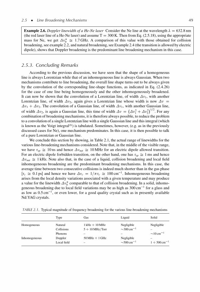
2.5 � Line Broadening Mechanisms 49
Example 2.6. Doppler linewidth of a He-Ne laser Consider the Ne line at the wavelength � D 632.8 nm(the red laser line of a He-Ne laser) and assume T D 300 K. Then from Eq. (2.5.18), using the appropriatemass for Ne, we get ��
0 Š 1.7 GHz. A comparison of this value with those obtained for collisionbroadening, see example 2.2, and natural broadening, see Example 2.4 (the transition is allowed by electricdipole), shows that Doppler broadening is the predominant line broadening mechanism in this case.
2.5.3. Concluding Remarks
According to the previous discussion, we have seen that the shape of a homogeneousline is always Lorentzian while that of an inhomogeneous line is always Gaussian. When twomechanisms contribute to line broadening, the overall line shape turns out to be always givenby the convolution of the corresponding line-shape functions, as indicated in Eq. (2.4.26)for the case of one line being homogeneously and the other inhomogeneously broadened.It can now be shown that the convolution of a Lorentzian line, of width �1, with anotherLorentzian line, of width �2, again gives a Lorentzian line whose width is now � D�1 C �2. The convolution of a Gaussian line, of width �1, with another Gaussian line,of width �2, is again a Gaussian line, this time of width � D
�21 C�2
2
�1=2. For any
combination of broadening mechanisms, it is therefore always possible, to reduce the problemto a convolution of a single Lorentzian line with a single Gaussian line and this integral (whichis known as the Voigt integral.9/) is tabulated. Sometimes, however, (e.g. as in the previouslydiscussed cases for Ne), one mechanism predominates. In this case, it is then possible to talkof a pure Lorentzian or Gaussian line.
We conclude this section by showing, in Table 2.1, the actual range of linewidths for thevarious line-broadening mechanisms considered. Note that, in the middle of the visible range,we have �sp Š 10 ns and hence �nat Š 10 MHz for an electric dipole allowed transition.For an electric dipole forbidden transition, on the other hand, one has �sp Š 1 ms and hence�nat Š 1 kHz. Note also that, in the case of a liquid, collision broadening and local fieldinhomogeneous broadening are the predominant broadening mechanisms. In this case, theaverage time between two consecutive collisions is indeed much shorter than in the gas phaseŒ�c Š 0.1 ps� and hence we have �c D 1= �c Š 100 cm�1. Inhomogeneous broadeningarises from the local density variations associated with a given temperature and may producea value for the linewidth ��
0 comparable to that of collision broadening. In a solid, inhomo-geneous broadening due to local field variations may be as high as 300 cm�1 for a glass andas low as 0.5 cm�1, or even lower, for a good quality crystal such as in presently availableNd:YAG crystals.
TABLE 2.1. Typical magnitude of frequency broadening for the various line-broadening mechanisms
Type Gas Liquid Solid
Homogeneous Natural 1 kHz � 10 MHz Negligible NegligibleCollisions 5 � 10 MHz=Torr �300 cm�1 –Phonons – – �10 cm�1
Inhomogeneous Doppler 50 MHz � 1 GHz Negligible –Local field – �500 cm�1 1 � 500 cm�1
50 2 � Interaction of Radiation with Atoms and Ions
2.6. NONRADIATIVE DECAY AND ENERGY TRANSFER
Besides decaying via radiative emission, an excited species can also undergo nonradia-tive decay. There exists a variety of ways by which this can occur and the detailed descriptionof the various physical phenomena can often be quite complicated. We shall therefore limitourselves to a qualitative discussion with the main aim being to elucidate the physical phe-nomena involved. We will then consider the combined effect of radiative and non-radiativedecay processes.
2.6.1. Mechanisms of Nonradiative Decay.10/
First we consider a nonradiative decay mechanism which arises from collisions, some-times called collisional deactivation. In this case, for a gas or a liquid, the transition energy isreleased as excitation and/or as kinetic energy of the colliding species or given to the walls ofthe container. In the case of a solid, such as an ionic crystal or glass, the energy of the excitedion is taken up by the lattice phonons or by the glass vibrational modes.
The collisional deactivation process, for the case where the energy of an excited speciesB� is released as kinetic energy of a colliding species A, can be expressed in the form
B� C A ! B C A CE (2.6.1)
whereE is equal to the excitation energy. SinceE ends up as kinetic energy of the collidingpartners, the process is also referred to as a superelastic collision or a collision of second kind.For a process of the form shown in Eq. (2.6.1), the rate of change of B� population, NB� , canbe written as
dNB�
dtD �kB�ANB� NA (2.6.2)
where NA is the population of species A and kB�A is a coefficient which depends on the transi-tion of species B and on species A. The process is particularly effective, i.e. kB�A is particularlylarge, when A has a very small mass (e.g. the He in the gas of a CO2 laser) so it can morereadily take-up the surplus energy E, from the collision process, as kinetic energy. For thesame reason the process can readily occur in a gas discharge when A is a discharge electron(e.g. deactivation of the 23S state of He in a He-Ne laser). According to Eq. (2.6.2), we cannow define a nonradiative decay rate
Wnr D kB�ANA (2.6.3)
From Eqs. (2.6.2) and (2.6.3) we then get
�dN2
dt
�D � N2
�nr(2.6.4)
where, to conform with previous notations, we have let N2 be the population of the speciesundergoing collisional deactivation and where we have defined a nonradiative decay time as�nr D .1=Wnr/.
2.6 � Nonradiative Decay and Energy Transfer 51
It should be observed that, in writing Eq. (2.6.2), we have neglected the reverse processof that given by Eq. (2.6.1) i.e.,
B C A ! B� C A �E (2.6.5)
where species B is excited at the expense of the kinetic energyE of the two colliding partners(thermal activation or collision of first kind). If this process were taken into account, oneshould write, instead of Eq. (2.6.2), the following equation
.dNB�=dt/ D �kB�ANB� NA C kBANBNA (2.6.6)
where kBA is a coefficient describing the process of thermal activation. To find the relationshipbetween kBA and kB�A we can consider species B in thermal equilibrium with species A andthen apply the so-called principle of detailed balance. This principle can generally be formu-lated by requiring that, in thermodynamic equilibrium, the rate of any process must be exactlybalanced by the rate of the corresponding reverse process�. Thus in this case, according toEq. (2.6.6), we require
kB�ANB� NA D kBANBNA (2.6.7)
In thermal equilibrium and for nondegenerate levels we have NB� D NB exp.�E=kT/ whereE is the excitation energy of species B and T is the temperature of the ensemble of speciesB and A. From Eq. (2.6.7) we then get
kB�A D kBA exp.E=kT/ (2.6.8)
which shows that the rate coefficient k for the exothermic reaction Eq. (2.6.1) is alwayslarger than that of the endothermic reaction Eq. (2.6.5). Actually, for electronic and for mostvibrational transitions, E is much larger than kT. Thus, according to Eq. (2.6.8), we havekB�A � kBA. It is very important also to realize that, although Eq. (2.6.8) has been derived forthermal equilibrium conditions, the same relation still holds if the population of species B ismaintained in a non equilibrium state of excitation, e.g. by some pumping process, providedthat the translational degrees of freedom of both species B and A are still in thermal equilib-rium. In fact, the quantum mechanical calculation of the rate coefficient k does not depend onthe population of B but only upon the eigenfunctions of the two species involved, and on theirrelative velocities. For a steady excitation of species B away from the Boltzmann equilibrium,i.e. when NB� is of the same order of NB, we thus have kB�ANB� � kBANB and Eq. (2.6.6)reduces to Eq. (2.6.2). Thus, to conclude, collisional deactivation takes the simple form givenby Eq. (2.6.4) only when E >> kT so that thermal activation may be neglected, whichis the case for electronic transitions and for most vibrational transitions. For deactivation ofthe lowest energy vibrational levels of some molecules [e.g. the (010) state of CO2] and forrotational transitions, thermal excitation must however be taken into account.
� Note that the equation expressing the balance of processes between a two level atom and the blackbody radiation,established in Sect. 2.4.4., is another example of the principle of detailed balance.
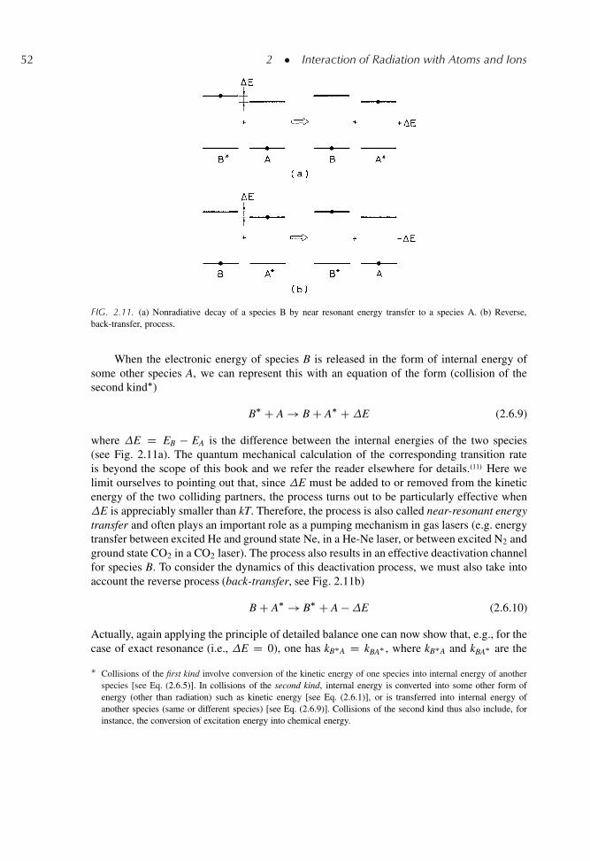
52 2 � Interaction of Radiation with Atoms and Ions
FIG. 2.11. (a) Nonradiative decay of a species B by near resonant energy transfer to a species A. (b) Reverse,back-transfer, process.
When the electronic energy of species B is released in the form of internal energy ofsome other species A, we can represent this with an equation of the form (collision of thesecond kind�)
B� C A ! B C A� CE (2.6.9)
where E D EB � EA is the difference between the internal energies of the two species(see Fig. 2.11a). The quantum mechanical calculation of the corresponding transition rateis beyond the scope of this book and we refer the reader elsewhere for details..11/ Here welimit ourselves to pointing out that, since E must be added to or removed from the kineticenergy of the two colliding partners, the process turns out to be particularly effective whenE is appreciably smaller than kT. Therefore, the process is also called near-resonant energytransfer and often plays an important role as a pumping mechanism in gas lasers (e.g. energytransfer between excited He and ground state Ne, in a He-Ne laser, or between excited N2 andground state CO2 in a CO2 laser). The process also results in an effective deactivation channelfor species B. To consider the dynamics of this deactivation process, we must also take intoaccount the reverse process (back-transfer, see Fig. 2.11b)
B C A� ! B� C A �E (2.6.10)
Actually, again applying the principle of detailed balance one can now show that, e.g., for thecase of exact resonance (i.e., E D 0), one has kB�A D kBA� , where kB�A and kBA� are the
� Collisions of the first kind involve conversion of the kinetic energy of one species into internal energy of anotherspecies [see Eq. (2.6.5)]. In collisions of the second kind, internal energy is converted into some other form ofenergy (other than radiation) such as kinetic energy [see Eq. (2.6.1)], or is transferred into internal energy ofanother species (same or different species) [see Eq. (2.6.9)]. Collisions of the second kind thus also include, forinstance, the conversion of excitation energy into chemical energy.
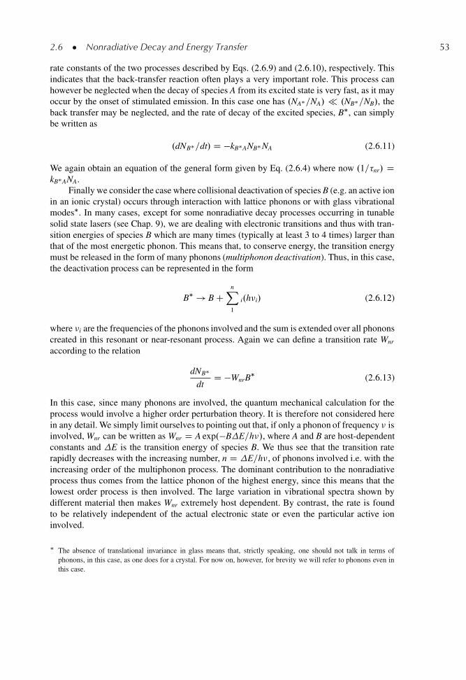
2.6 � Nonradiative Decay and Energy Transfer 53
rate constants of the two processes described by Eqs. (2.6.9) and (2.6.10), respectively. Thisindicates that the back-transfer reaction often plays a very important role. This process canhowever be neglected when the decay of species A from its excited state is very fast, as it mayoccur by the onset of stimulated emission. In this case one has .NA�=NA/ � .NB�=NB/, theback transfer may be neglected, and the rate of decay of the excited species, B�, can simplybe written as
.dNB�=dt/ D �kB�ANB� NA (2.6.11)
We again obtain an equation of the general form given by Eq. (2.6.4) where now .1=�nr/ DkB�ANA.
Finally we consider the case where collisional deactivation of species B (e.g. an active ionin an ionic crystal) occurs through interaction with lattice phonons or with glass vibrationalmodes�. In many cases, except for some nonradiative decay processes occurring in tunablesolid state lasers (see Chap. 9), we are dealing with electronic transitions and thus with tran-sition energies of species B which are many times (typically at least 3 to 4 times) larger thanthat of the most energetic phonon. This means that, to conserve energy, the transition energymust be released in the form of many phonons (multiphonon deactivation). Thus, in this case,the deactivation process can be represented in the form
B� ! B CnX1
i.h�i/ (2.6.12)
where �i are the frequencies of the phonons involved and the sum is extended over all phononscreated in this resonant or near-resonant process. Again we can define a transition rate Wnr
according to the relation
dNB�
dtD �WnrB
� (2.6.13)
In this case, since many phonons are involved, the quantum mechanical calculation for theprocess would involve a higher order perturbation theory. It is therefore not considered herein any detail. We simply limit ourselves to pointing out that, if only a phonon of frequency � isinvolved, Wnr can be written as Wnr D A exp.�BE=h�/, where A and B are host-dependentconstants and E is the transition energy of species B. We thus see that the transition raterapidly decreases with the increasing number, n D E=h�, of phonons involved i.e. with theincreasing order of the multiphonon process. The dominant contribution to the nonradiativeprocess thus comes from the lattice phonon of the highest energy, since this means that thelowest order process is then involved. The large variation in vibrational spectra shown bydifferent material then makes Wnr extremely host dependent. By contrast, the rate is foundto be relatively independent of the actual electronic state or even the particular active ioninvolved.
� The absence of translational invariance in glass means that, strictly speaking, one should not talk in terms ofphonons, in this case, as one does for a crystal. For now on, however, for brevity we will refer to phonons even inthis case.
54 2 � Interaction of Radiation with Atoms and Ions
As a conclusion to this discussion on collisional deactivation, we note that, while theprocess can take a variety of forms, the decay behavior of the excited state can, subjects tolimits that we have discussed, always be described by the general relation Eq. (2.6.4), wherethe value of �nr will depend upon the particular process under consideration. It should benoted explicitly, however, that there is a fundamental difference between the nonradiativedecay time, �nr, discussed here, and the collision time �c discussed in Sect. 2.5.1, althoughthey both originate from collisions. In fact, a nonradiative decay process requires an inelasticcollision since the decaying species gives up its energy to its surroundings. By contrast, �c isthe average time between two consecutive dephasing collisions and thus arises from elasticcollisions only. Note that, in general, elastic collisions are more likely than inelastic ones andthus �c is smaller, and often much smaller, than �nr .
A kind of nonradiative decay that does not rely on collisions, arises from dipole-dipoleinteraction between an excited species that we shall call the donor, D, and, e.g., a groundstate species that we shall call the acceptor, A. The interaction results in energy being trans-ferred between donor and acceptor. This process has been extensively studied by Forster forliquids.12/ and by Dexter for solids..13/ It plays a very important role e.g. for active ions incrystals or glasses and for mixtures of organic dyes in solution. Consider the donor, undergo-ing the downward transition, while at a distance R from the acceptor. During the transition,the donor will develop a dipole moment, μD, oscillating at its transition frequency. From thetheory of electric dipole radiation,.14/ it is known that this moment generates, at a distance R,a nonradiating electric field (the so called near-zone field) whose magnitude, ED.t/, as for anelectrostatic dipole, is equal to μD=4 "0R3. Under these conditions, nonradiative decay mayoccur by energy transfer arising from the interaction of the near-zone field ED.t, R/ at the posi-tion of the acceptor with the oscillating dipole moment of the acceptor, μA. The interactionenergy, H, can then be written as
H / jED � μAj / jμD � μAj=R3 (2.6.14)
Of course, the interaction will have a significant strength only if the oscillation frequency ofμD is nearby resonant with that of μA. This means that there should be a good overlap betweenthe emission spectrum of the donor and the absorption spectrum of the acceptor from its initialstate (often not necessarily being the ground state). The detailed calculation shows that, for asingle donor and acceptor separated by a distance R, the rate of energy transfer can be writtenas.12/
WDA D�
3
64 5
��1
R6
�24 1
�sp
1Z0
� c
n�
�4gD.�/�A.�/d�
35 (2.6.15)
where �sp is the spontaneous lifetime of the donor, n is the refractive index of the surroundingmedium gD is the line-shape function of the donor and �A is the absorption cross-section ofthe acceptor. Note that since, as usual, the dependence of WDA with the interaction energy His WDA / jHj2, from Eq. (2.6.14) we expect WDA / j�Dj2j�Aj2=R6. By this relation one canunderstand the dependence of WDA not only from R�6 but also from .1=�sp/ [remember that1=�sp / jμDj2, see Eq. (2.3.15)] and to the cross section �A of the acceptor [remember that�A / jμAj2, see Eq. (2.4.29)].
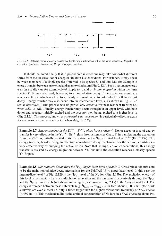
2.6 � Nonradiative Decay and Energy Transfer 55
FIG. 2.12. Different forms of energy transfer by dipole-dipole interaction within the same species: (a) Migration ofexcitation. (b) Cross relaxation. (c) Cooperative up-conversion.
It should be noted finally that, dipole-dipole interactions may take somewhat differentforms from the classical donor-acceptor situation just considered. For instance, it may occurbetween members of a single species (referred to as species D) and thus lead for example toenergy transfer between an excited and an unexcited atom [Fig. 2.12a]. Such a resonant energytransfer usually can, for example, lead simply to spatial excitation migration within the samespecies D. It may also lead, however, to a nonradiative decay if the excitation eventuallyreaches a D site which is close to a, nearly resonant, acceptor site which itself has a fastdecay. Energy transfer may also occur into an intermediate level, i, as shown in Fig. 2.12b(cross relaxation). This process will be particularly effective for near resonant transfer i.e.when E2i Š Ei1. Finally, energy transfer may occur throughout an upper level, with bothdonor and acceptor initially excited and the acceptor then being excited to a higher level u(Fig. 2.12c). This process, known as cooperative up-conversion, is particularly effective againfor near resonant energy transfer i.e. when E2u Š E21.
Example 2.7. Energy transfer in the Yb3C : Er3C: glass laser system.15/ Donor-acceptor type of energytransfer is very effective in the Yb3C : Er3C:glass laser system (see Chap. 9) in transferring the excitationfrom the Yb3 ion, initially excited to its 2F5=2 state, to the 4I11=2 excited level of Er3C (Fig. 2.13a). Thisenergy transfer, besides being an effective nonradiative decay mechanism for the Yb ion, constitutes avery effective way of pumping the active Er ion. Note that, at high Yb ion concentrations, this energytransfer is assisted by energy migration between Yb ions until the excitation reaches a closely spacedYb-Er pair.
Example 2.8. Nonradiative decay from the 4F3=2 upper laser level of Nd:YAG Cross relaxation turns outto be the main nonradiative decay mechanism for the Nd:YAG 4F3=2 upper laser level. In this case theintermediate level i of Fig. 2.12b is the 4I15=2 level of the Nd ion (Fig. 2.13b). The excitation energy ofthis level is then rapidly lost via multiphonon relaxation and the ion passes successively through the 4I13=2
and the 4I11=2 lower levels (not shown in the figure, see however Fig. 2.15) to the 4I9=2 ground level. Theenergy difference between these sublevels (e.g. 4I13=2 ! 4I11=2) is, in fact, about 2, 000 cm�1 (the Starksublevels are even closer) i.e. only 4 times larger than the highest vibrational frequency of YAG crystal.�450 cm�1/. This mechanism limits the optimal concentration of Nd ions in a YAG crystal to about 1%.
56 2 � Interaction of Radiation with Atoms and Ions
FIG. 2.13. Examples of energy transfer by dipole-dipole interaction: (a) Yb3C � Er3C energy transfer in an Yb:Erlaser or amplifier. (b) Nonradiative decay of Nd:YAG by cross relaxation. (c) Cooperative upconversion in an Er3C
laser or amplifier.
Example 2.9. Cooperative upconversion in Er3C lasers and amplifiers.15/ Cooperative up-conversion isbelieved to be the major cause of inefficiency for Er3C lasers or amplifiers (Fig. 2.13c). In this case, outof two neighboring Er ions initially excited to the 4I13=2 laser level, one decays to the ground 4I15=2 levelwhile the other is raised to the 4I9=2 level. From this level the ion, when in an oxide glass host, then decaysrapidly back to the 4I13=2 level by multiphonon decay. The net result of this cooperative up-conversion isthat one Er ion, initially excited to the laser 4I13=2 level, is effectively quenched to the ground level i.e.,one looses 50% of the population.
2.6.2. Combined Effects of Radiative and Nonradiative Processes
Let us first consider the case where the nonradiative decay can be described by an equa-tion of the general form Eq. (2.6.4). The time variation of the upper state population N2 canthen be written as
dN2
dtD �
�N2
�rC N2
�nr
�(2.6.16)
Equation (2.6.16) can be put in the simpler form
dN2=dt D �.N2=�/ (2.6.17)
provided that one defines an overall decay time � given by
1
�D 1
�rC 1
�nr(2.6.18)
The population N2.t/ at time t is then obtained by integrating Eq. (2.6.17). We get
N2.t/ D N2.0/ exp �.t=�/ (2.6.19)
2.6 � Nonradiative Decay and Energy Transfer 57
where N2.0/ is the population at t D 0. To calculate the time behavior of the spontaneouslyemitted light, we notice that, according to Eq. (2.6.16), N2=�r gives the number of atomsdecaying radiatively per unit volume and unit time. Assuming, for simplicity, that radiativedecay occurs to one lower level only, say level 1, and letting �0 be the corresponding transitionfrequency, the spontaneously emitted power at time t will then be
P.t/ D N2.t/h�0V=�r (2.6.20)
where V is the volume of the material. With the help of Eq. (2.6.19), Eq. (2.6.20) gives
P.t/ D ŒN2.0/h�0V=�r� exp �.t=�/ (2.6.21)
Note that the time decay of the emitted light is exponential with a time constant � ratherthan �r as one, perhaps, might have expected at a first sight. By monitoring the decay of thespontaneously emitted light from a sample having, at t D 0, an initial upper state populationN2.0/, one thus measures the overall lifetime � . To obtain �r, let us first define the fluorescencequantum yield � as the ratio of the number of emitted photons to the number of atoms initiallyraised to level 2. Using Eq. (2.6.21), we have
� DR.P.t/=h�0/dt
N2.0/VD �
�r(2.6.22)
Note that one can easily show that the above relation remains true also when the decay is intoa number of lower levels provided that, in defining the quantum efficiency �, one includes thephotons emitted in all of these transitions. The measurement of � thus allows calculation of�r once � is known from the decay measurement of the emitted radiation. This measurement,however, is sometimes not an easy one especially when � is very short (picoseconds or evenless), i.e. when � is very small.
We now briefly consider the case in which nonradiative decay occurs via a dipole-dipole mediated energy transfer. According to Eq. (2.6.15), the transition rate WDA is stronglydependent upon the donor to acceptor distance, R. For a population of ND donors and NA
acceptors, due to the different distances between donors and acceptors, the decay rate willbe different from each donor to acceptor couple and the resulting overall decay will showa non-exponential behavior, the initial faster decay corresponding to sites with the smallestseparation R. A particularly important case occurs where there are random values of the donor-acceptor spacing and where this distance is either fixed, as in a solid, or slowly varying over aspontaneous decay time, as often occurs for liquids (Forster regime). In this case, when bothradiative and nonradiative decay channels are taken into account, the overall decay is given by
N2.t/ D N2.0/ exp �h.t=�r/C Ct1=2
i(2.6.23)
The time behavior of the radiated power is then obtained by substituting Eq. (2.6.23) intoEq. (2.6.20) and thus follows the same non-exponential decay as that of the population N2.t/.
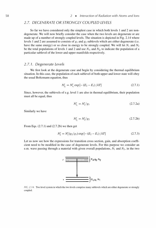
58 2 � Interaction of Radiation with Atoms and Ions
2.7. DEGENERATE OR STRONGLY COUPLED LEVELS
So far we have considered only the simplest case in which both levels 1 and 2 are non-degenerate. We will now briefly consider the case when the two levels are degenerate or aremade up of a number of strongly coupled levels. The situation is depicted in Fig. 2.14 wherelevels 1 and 2 are assumed to consists of g1 and g2 sublevels which are either degenerate (i.e.have the same energy) or so close in energy to be strongly coupled. We will let N1 and N2
be the total populations of levels 1 and 2 and use N1i and N2j to indicate the population of aparticular sublevel of the lower and upper manifolds respectively.
2.7.1. Degenerate Levels
We first look at the degenerate case and begin by considering the thermal equilibriumsituation. In this case, the population of each sublevel of both upper and lower state will obeythe usual Boltzmann equation, thus
Ne2j
D Ne1i
exp Œ� .E2 � E1/ =kT� (2.7.1)
Since, however, the sublevels of e.g. level 1 are also in thermal equilibrium, their populationmust all be equal, thus
Ne1i
D Ne1=g1 (2.7.2a)
Similarly we have
Ne2j
D Ne2=g2 (2.7.2b)
From Eqs. (2.7.1) and (2.7.2b) we then get
Ne2 D Ne
1.g2=g1/ exp Œ� .E2 � E1/ =kT� (2.7.3)
Let us now see how the expressions for transition cross section, gain, and absorption coeffi-cient need to be modified in the case of degenerate levels. For this purpose we consider ane.m. wave passing through a material with given overall populations, N1 and N2, in the two
FIG. 2.14. Two level system in which the two levels comprise many sublevels which are either degenerate or stronglycoupled.
2.7 � Degenerate or Strongly Coupled Levels 59
levels, and we calculate the rate of change of the overall population N2 due to all radiative andnonradiative transitions between sublevels j and i. We therefore write
�dN2
dt
�D �
g1X1
i
g2X1
j
�WjiN2j � WijN1i C N2j
�ji
�(2.7.4)
where Wji is the rate of stimulated transition between j and i sublevels, Wij is the rate ofabsorption and .1=τji/ is the rate of spontaneous decay, radiative and nonradiative, betweenthe same two sublevels. Note that Wji and Wij are obtained from Eq. (2.4.30) by substitutingthe dipole moments between j and i sublevels, j�ijj2 and j�jij2, for j�j2. These dipole momentscan in turn be readily obtained from Eq. (2.3.7). For instance j�ijj is obtained from Eq. (2.3.7)by substituting ui, the eigenfunction of the i-th lower level, for u1 and uj, the eigenfunction ofthe j-th upper level, for u2. It then follows that:
Wji D Wij (2.7.5)
If a rapid relaxation towards thermal equilibrium occurs between the sublevels within eachlevel, then all sublevels of the upper level will again be equally populated, and the same willoccur to the sublevels of the lower level. Therefore
N2j D N2=g2 (2.7.6a)
N1i D N1=g1 (2.7.6b)
Upon substitution of Eq. (2.7.6) into Eq. (2.7.4) we then get
dN2
dtD �W
�N2
g2� N1
g1
�� N2
�(2.7.7)
where, with the help of Eq. (2.7.5), we have defined
W Dg1X1
i
g2X1
j Wij Dg1X1
i
g2X1
jWji (2.7.8)
and
1
�D
g1P1
i
g2P1
j1=�ji
�g2
(2.7.9)
From Eq. (2.7.7) one can observe now that WN2=g2 represents the change in the unit timeof the total upper state population due to all stimulated emissions processes and, likewise,WN1=g1 represents the population change due to all absorption processes. The change inphoton flux dF when the beam travels a distance dz in the material (see Fig. 1.2) can then bewritten as
dF D W
�N2
g2� N1
g1
�dz (2.7.10)
60 2 � Interaction of Radiation with Atoms and Ions
We can now define a stimulated emission cross section, �21, and absorption cross section,�12, as
�21 D W=.g2F/ (2.7.11a)
�12 D W=.g1F/ (2.7.11b)
from which we obviously have
g2�21 D g1�12 (2.7.12)
When .N1=g1/ > .N2=g2/ Eq. (2.7.10) with the help of Eq. (2.7.11b) can be put in the familiarform dF D �˛Fdz provided one defines the absorption coefficient ˛ as
˛ D �12
�N1 � N2
g1
g2
�(2.7.13)
Similarly, when .N2=g2/ > .N1=g1/, Eq. (2.7.10) with the help of Eq. (2.7.11a) can be put inthe familiar form dF D gFdz provided one defines the gain coefficient g as
g D �21
�N2 � N1
g2
g1
�(2.7.14)
The reasons for defining �21 and �12, respectively, as in Eqs. (2.7.11a) and (2.7.11b) is nowapparent. When in fact N1 � N2 (as usually applies to absorption measurements involvingoptical transitions) Eq. (2.7.13) simply reduces to ˛ D �12N1. Conversely, when N2 � N1 (asapplies in a four-level laser), Eq. (2.7.14) simply reduces to g D �21N2.
2.7.2. Strongly Coupled Levels
We now turn to the case where the upper level, 2, and lower level, 1, actually consist ofg2 and g1 sublevels, respectively, with different energies but with very fast relaxation amongthe sublevels belonging to each particular level (strongly coupled levels). Each sublevel, ofboth upper and lower levels, may also consists, itself, of many degenerate levels. In thiscase, thermalization among the sublevels of either lower and upper level will occur rapidlyso that we can assume Boltzmann’s statistics to be always obeyed. Instead of Eq. (2.7.6), wewrite now
N2j D f2j N2 (2.7.15a)
N1i D f1i N1 (2.7.15b)
2.7 � Degenerate or Strongly Coupled Levels 61
where f2j .f1i/ is the fraction of total population of level 2 (level 1) that, at thermal equilibrium,is found in sublevel j.i/. According to Boltzmann’s statistics, we then have
f2j D g2j exp �.E2j=kT/g2P1
mg2m exp �.E2m=kT/(2.7.16a)
f1i D g1i exp �.E1i=kT/g1P1
lg1l exp �.E1l=kT/(2.7.16b)
where E2m and E1l are the energies of the sublevels in the upper and lower level, respectivelyand g2m and g1l are the corresponding degeneracies.
Let us now assume that the stimulated transition occurs between a given sublevel (say l)of level 1 to a given sublevel (say m) of level 2. Equation (2.7.4) then simplifies to
�dN2
dt
�D �WmlN2m C WlmN1l �
g1X1
i
g2X1
j
�N2j
�ji
�(2.7.17)
With the help of Eq. (2.7.15), Eq. (2.7.17) can be written as
.dN2=dt/ D �WemlN2 C We
lmN1 � .N2=�/ (2.7.18)
where we have defined the effective rates of stimulated emission, Weml, stimulated absorption,
Walm, and spontaneous decay, .1=�/, respectively as
Weml D f2m Wml (2.7.19a)
Walm D f1l Wlm (2.7.19b)
.1=�/ Dg1X1
i
g2X1
j.f2j=�ji/ (2.7.19c)
According to Eq. (2.7.18), the change in photon flux dF when the beam travels a distance dzin the material is given now
dF D We
mlN2 � WalmN1
�dz (2.7.20)
We can then define an effective stimulated emission cross section, �eml, and an effective
absorption cross section, �alm, as
�eml D We
ml=F D f2m�lm (2.7.21a)
�aml D Wa
ml=F D f1l�lm (2.7.21b)
where Eqs. (2.7.19a) and (2.7.19b) have been used and where �lm D Wlm=F and �ml D Wml=Fare, respectively, the effective cross sections of absorption and stimulated emission for the l
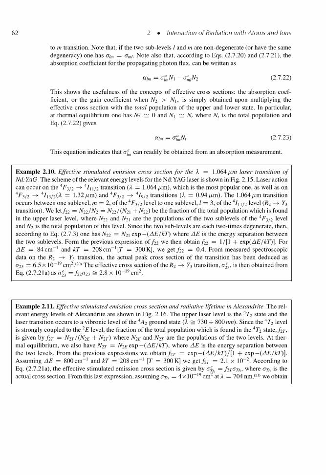
62 2 � Interaction of Radiation with Atoms and Ions
to m transition. Note that, if the two sub-levels l and m are non-degenerate (or have the samedegeneracy) one has �lm D �ml. Note also that, according to Eqs. (2.7.20) and (2.7.21), theabsorption coefficient for the propagating photon flux, can be written as
˛lm D �almN1 � �e
mlN2 (2.7.22)
This shows the usefulness of the concepts of effective cross sections: the absorption coef-ficient, or the gain coefficient when N2 > N1, is simply obtained upon multiplying theeffective cross section with the total population of the upper and lower state. In particular,at thermal equilibrium one has N2 Š 0 and N1 Š Nt where Nt is the total population andEq. (2.7.22) gives
˛lm D �almNt (2.7.23)
This equation indicates that �elm can readily be obtained from an absorption measurement.
Example 2.10. Effective stimulated emission cross section for the � D 1.064�m laser transition ofNd:YAG The scheme of the relevant energy levels for the Nd:YAG laser is shown in Fig. 2.15. Laser actioncan occur on the 4F3=2 ! 4I11=2 transition .� D 1.064�m/, which is the most popular one, as well as on4F3=2 ! 4I13=2.� D 1.32�m/ and 4F3=2 ! 4I9=2 transitions .� D 0.94�m/. The 1.064�m transitionoccurs between one sublevel, m D 2, of the 4F3=2 level to one sublevel, l D 3, of the 4I11=2 level (R2 ! Y3
transition). We let f22 D N22=N2 D N22=.N21 C N22/ be the fraction of the total population which is foundin the upper laser level, where N22 and N21 are the populations of the two sublevels of the 4F3=2 leveland N2 is the total population of this level. Since the two sub-levels are each two-times degenerate, then,according to Eq. (2.7.3) one has N22 D N21 exp �.E=kT/ where E is the energy separation betweenthe two sublevels. Form the previous expression of f22 we then obtain f22 D 1=Œ1 C exp.E=kT/�. ForE D 84 cm�1 and kT D 208 cm�1ŒT D 300 K�, we get f22 D 0.4. From measured spectroscopicdata on the R2 ! Y3 transition, the actual peak cross section of the transition has been deduced as�23 D 6.5�10�19 cm2..20/ The effective cross section of the R2 ! Y3 transition, �e
23, is then obtained fromEq. (2.7.21a) as �e
23 D f22�23 Š 2.8 � 10�19 cm2.
Example 2.11. Effective stimulated emission cross section and radiative lifetime in Alexandrite The rel-evant energy levels of Alexandrite are shown in Fig. 2.16. The upper laser level is the 4T2 state and thelaser transition occurs to a vibronic level of the 4A2 ground state .� Š 730 � 800 nm/. Since the 4T2 levelis strongly coupled to the 2E level, the fraction of the total population which is found in the 4T2 state, f2T ,is given by f2T D N2T=.N2E C N2T / where N2E and N2T are the populations of the two levels. At ther-mal equilibrium, we also have N2T D N2E exp �.E=kT/, where E is the energy separation betweenthe two levels. From the previous expressions we obtain f2T D exp �.E=kT/=Œ1 C exp �.E=kT/�.Assuming E D 800 cm�1 and kT D 208 cm�1 ŒT D 300 K� we get f2T D 2.1 � 10�2. According toEq. (2.7.21a), the effective stimulated emission cross section is given by �e
TA D f2T�TA, where �TA is theactual cross section. From this last expression, assuming �TA D 4�10�19 cm2 at � D 704 nm,.21/ we obtain
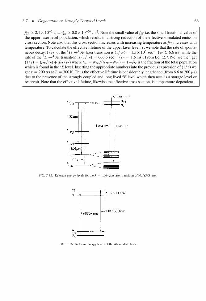
2.7 � Degenerate or Strongly Coupled Levels 63
f2T Š 2.1 � 10�2 and �eTA Š 0.8 � 10�20 cm2. Note the small value of f2T i.e. the small fractional value of
the upper laser level population, which results in a strong reduction of the effective stimulated emissioncross section. Note also that this cross section increases with increasing temperature as f2T increases withtemperature. To calculate the effective lifetime of the upper laser level, � , we note that the rate of sponta-neous decay, 1=�T , of the 4T2 !4 A2 laser transition is .1=�T/ D 1.5 � 105 sec�1 .�T Š 6.6�s/ while therate of the 2E !4 A2 transition is .1=�E/ D 666.6 sec�1 .�E D 1.5 ms/. From Eq. (2.7.19c) we then get.1=�/ D .f2E=�E/C.f2T=�T/ where f2E D N2E=.N2E CN2T/ D 1� f2T is the fraction of the total populationwhich is found in the 2E level. Inserting the appropriate numbers into the previous expression of .1=�/ weget � D 200�s at T D 300 K. Thus the effective lifetime is considerably lengthened (from 6.6 to 200�s)due to the presence of the strongly coupled and long lived 2E level which then acts as a storage level orreservoir. Note that the effective lifetime, likewise the effective cross section, is temperature dependent.
FIG. 2.15. Relevant energy levels for the � D 1.064�m laser transition of Nd:YAG laser.
FIG. 2.16. Relevant energy levels of the Alexandrite laser.
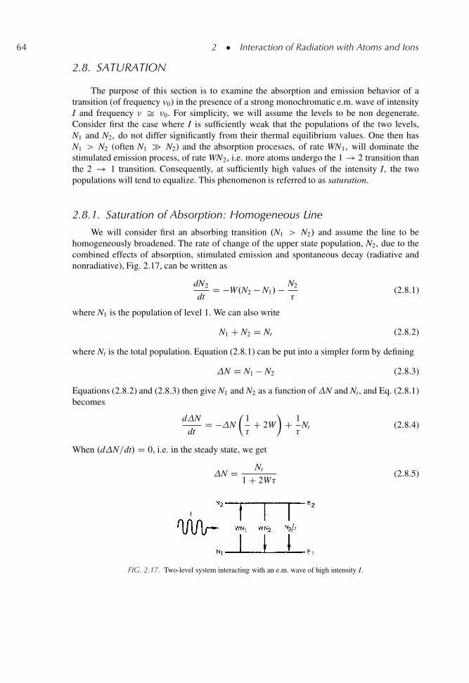
64 2 � Interaction of Radiation with Atoms and Ions
2.8. SATURATION
The purpose of this section is to examine the absorption and emission behavior of atransition (of frequency �0) in the presence of a strong monochromatic e.m. wave of intensityI and frequency � Š �0. For simplicity, we will assume the levels to be non degenerate.Consider first the case where I is sufficiently weak that the populations of the two levels,N1 and N2, do not differ significantly from their thermal equilibrium values. One then hasN1 > N2 (often N1 � N2) and the absorption processes, of rate WN1, will dominate thestimulated emission process, of rate WN2, i.e. more atoms undergo the 1 ! 2 transition thanthe 2 ! 1 transition. Consequently, at sufficiently high values of the intensity I, the twopopulations will tend to equalize. This phenomenon is referred to as saturation.
2.8.1. Saturation of Absorption: Homogeneous Line
We will consider first an absorbing transition .N1 > N2/ and assume the line to behomogeneously broadened. The rate of change of the upper state population, N2, due to thecombined effects of absorption, stimulated emission and spontaneous decay (radiative andnonradiative), Fig. 2.17, can be written as
dN2
dtD �W.N2 � N1/� N2
�(2.8.1)
where N1 is the population of level 1. We can also write
N1 C N2 D Nt (2.8.2)
where Nt is the total population. Equation (2.8.1) can be put into a simpler form by defining
N D N1 � N2 (2.8.3)
Equations (2.8.2) and (2.8.3) then give N1 and N2 as a function of N and Nt, and Eq. (2.8.1)becomes
dN
dtD �N
�1
�C 2W
�C 1
�Nt (2.8.4)
When .dN=dt/ D 0, i.e. in the steady state, we get
N D Nt
1 C 2W�(2.8.5)
FIG. 2.17. Two-level system interacting with an e.m. wave of high intensity I.
2.8 � Saturation 65
To maintain a given population difference,N, the material needs to absorb from the incidentradiation a power per unit volume (dP/dV) given by
dP
dVD .h�/WN D .h�/
NtW
1 C 2W�(2.8.6)
which, at saturation, i.e., for W� � 1, becomes
.dP=dV/s D .h�/Nt=2� (2.8.7)
Equation (2.8.7) shows that the power that must be absorbed by the system to keep it insaturation, .dP=dV/s, is, as expected, equal to the power lost by the material due to the decayof the upper state population .Nt=2/.
It is sometimes useful to have Eqs. (2.8.5) and (2.8.6) rewritten in a more convenientform. To do this we first notice that, according to Eq. (2.4.17), W can be expressed as
W D �I=h� (2.8.8)
where � is the absorption cross section of the transition. Equations (2.8.5) and (2.8.6) withthe help of Eq. (2.8.8) can be recast in the following forms:
N
NtD 1
1 C .I=Is/(2.8.9)
dP=dV
.dP=dV/sD I=Is
1 C .I=Is/(2.8.10)
where
Is D h�=2�� (2.8.11)
is a parameter that depends on the given material and on the frequency of the incident wave.Its physical meaning is obvious from Eq. (2.8.9). In fact, for I D Is, we getN D Nt=2. When� D �0, the quantity Is has a value that depends only on the parameters of the transition. Thisquantity is called the saturation intensity.
Let us now see how the shape of an absorption line changes with increasing value ofthe intensity, I, of the saturating beam. To do this, consider the idealized experimental situ-ation shown in Fig. 2.18 where the absorption measurements are made using a probe beamof variable frequency � 0 and whose intensity I0 is small enough so as not to perturb the sys-tem appreciably. In practice the beams need to be more or less collinear to ensure that theprobe beam interacts only with the saturated region. Under these conditions, the absorptioncoefficient as seen by the probe beam is obtained from Eq. (2.4.33) by substituting the totallineshape gt.���0/ with the homogeneous lineshape g.�0 ��0/, where � has been substitutedby �0. Since N1 � N2 D N is now given by Eq. (2.8.9), we can write
˛ D ˛0
1 C .I=Is/(2.8.12)
66 2 � Interaction of Radiation with Atoms and Ions
FIG. 2.18. Measurement of the absorption or gain coefficient at frequency �0, by a probe beam of intensity I0.�0/ inthe presence of a saturating beam, I.�/, of intensity I and frequency �ŒI.�/ � I0.�0/�.
FIG. 2.19. Saturation behavior of the absorption coefficient, ˛, vs frequency, �0, for increasing values of theintensity, I, of the saturating beam (homogeneous line).
where
˛0 D 2 2
3n"0chj�j2 Nt�
0g.�0 � �0/ (2.8.13)
is the absorption coefficient when the saturating wave at frequency � is absent (unsaturatedabsorption coefficient). Equations (2.8.12) and (2.8.13) show that, when the intensity I of thesaturating beam is increased, the absorption coefficient is reduced. The line shape, however,remains the same since it is always described by the function g.�0 � �0/. Figure 2.19 showsthree plots of the absorption coefficient ˛ vs �0 at three different values of I=Is.
We next consider the case where the saturating e.m. wave consists of a light pulse withintensity I D I.t/, rather than a cw beam. For simplicity, we will confine ourselves to acomparison between two limiting cases in which the pulse duration is either very long or veryshort compared to the upper state lifetime � . If the pulse duration is very long compared to thelifetime, the time evolution of the resulting population difference N, due to saturation, willoccur at very slow rate so that we can assume in Eq. (2.8.4) dN=dt � Nt=� . Accordingly,N turns out to be still given by the steady state Eq. (2.8.9) where now I D I.t/. The saturationbehavior in this case is essentially the same as for a cw beam. If, on the other hand, the lightpulse is very short compared to the lifetime � , then the absorption term �2WN in Eq. (2.8.4)dominates the spontaneous decay term .Nt � N/=� , i.e. Œ.Nt � N/=�� � 2WN. In thiscase Eq. (2.8.4) reduces to
.dN=dt/ D �2WN D �.2�=h�/I.t/N (2.8.14)
2.8 � Saturation 67
where Eq. (2.8.8) has also been used. Integration of Eq. (2.8.14) with the initial conditionN.0/ D Nt gives
N.t/ D Nt exp
24�.2�=h�/
tZ0
I.t/dt
35 (2.8.15)
Equation (2.8.15) can be put in a more suggestive form if we define the energy fluence � .t/ as
� .t/ DtZ
0
I.t/dt (2.8.16)
and the saturation fluence as
�s D h�=2� (2.8.17)
From Eq. (2.8.15) we then get
N.t/ D Nt exp � Œ� .t/=�s� (2.8.18)
We see that, in this case, it is the beam energy fluence rather than its intensity that determinesthe saturation behavior. The population difference N1 that is left in the material after thepulse has passed is, according to Eq. (2.8.18), given by
N1 D Nt exp �.�t=�s/ (2.8.19)
where �t is the total energy fluence of the light pulse. The material saturation fluence �s cantherefore be looked upon as the fluence that the pulse should have to produce a population dif-ference N1 D Nt=e. Having calculated the population difference resulting from saturationby a light pulse, the corresponding absorption coefficient of the material can then be obtained,for a homogeneous line, again from Eq. (2.4.33) by substituting gt.� � �0/ with g.�0 � �0/.For a light pulse that is, either, slow or fast compared to � , the value of ˛ is respectively givenby Eq. (2.8.12) [with I D I.t/] or by
˛ D ˛0 exp Œ��.t/=�s� (2.8.20)
where ˛0 is the unsaturated absorption coefficient. Note that, in the pulsed regime as in thecw regime, the shape of the absorption line remains unchanged when saturation occurs.
2.8.2. Gain Saturation: Homogeneous Line
We now consider the case where the transition 2 ! 1 exhibits net gain rather than netabsorption. We assume that the medium behaves as a four-level system (Fig. 2.20) and theinversion between levels 2 and 1 is produced by some suitable pumping process. We willfurther assume that the 3 ! 2 and 1 ! g transitions are so fast that we can take N3 Š
68 2 � Interaction of Radiation with Atoms and Ions
FIG. 2.20. Energy levels and transitions involved in gain saturation of a four-level laser.
N1 Š 0. With these simplifying assumptions we can write the following rate equation for thepopulation of level 2:
.dN2=dt/ D Rp � WN2 � .N2=�/ (2.8.21)
where Rp is the pumping rate and Nt is the total population. In the steady state (i.e., fordN2=dt D 0) we find from Eq. (2.8.21)
N2 D Rp�
1 C W�(2.8.22)
With the help of Eq. (2.8.8), Eq. (2.8.22) can be rewritten as
N2 D N20
1 C .I=Is/(2.8.23)
where N20 D Rp� is the population of level 2 in the absence of the saturating beam (i.e. forI D 0) and
Is D h�=�� (2.8.24)
A comparison of Eq. (2.8.24) with Eq. (2.8.11) shows that the expression for the saturationintensity Is of a four-level system is twice that of the two-level system of Fig. 2.17. Thedifference arises from the fact that, in a two-level system, a change in population of one levelcauses an equal and opposite change in population in the other level. Thus N is twice thechange in population of each level.
In an experiment such as that shown in Fig. 2.18, the probe beam at frequency �0 will nowmeasure gain rather than absorption. From Eq. (2.4.35), with N1 D 0, using also Eq. (2.8.23),the gain coefficient, g, can be written as
g D g0
1 C .I=Is/(2.8.25)
where g0 D �N20 is the gain coefficient for I D 0, i.e. when the saturating beam isabsent (unsaturated gain coefficient). This gain coefficient, since the line is homogeneouslybroadened, can be obtained, using Eq. (2.4.18), as
g0 D 2 2
3n"0chj�j2�0N20g.�0 � �0/ (2.8.26)
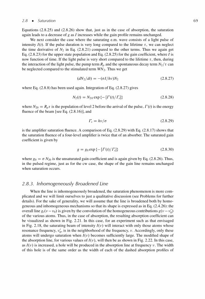
2.8 � Saturation 69
Equations (2.8.25) and (2.8.26) show that, just as in the case of absorption, the saturationagain leads to a decrease of g as I increases while the gain profile remains unchanged.
We next consider the case where the saturating e.m. wave consists of a light pulse ofintensity I.t/. If the pulse duration is very long compared to the lifetime � , we can neglectthe time derivative of N2 in Eq. (2.8.21) compared to the other terms. Thus we again getEq. (2.8.23) for the upper state population and Eq. (2.8.25) for the gain coefficient, where I isnow function of time. If the light pulse is very short compared to the lifetime � , then, duringthe interaction of the light pulse, the pump term Rp and the spontaneous decay term N2=� canbe neglected compared to the stimulated term WN2. Thus we get
.dN2=dt/ D �.�I=h�/N2 (2.8.27)
where Eq. (2.8.8) has been used again. Integration of Eq. (2.8.27) gives
N2.t/ D N2 0 exp f� Œ� .t/=�s�g (2.8.28)
where N20 D Rp� is the population of level 2 before the arrival of the pulse, � .t/ is the energyfluence of the beam [see Eq. (2.8.16)], and
�s D h�=� (2.8.29)
is the amplifier saturation fluence. A comparison of Eq. (2.8.29) with Eq. (2.8.17) shows thatthe saturation fluence of a four-level amplifier is twice that of an absorber. The saturated gaincoefficient is given by
g D g0 exp f� Œ� .t/=�s�g (2.8.30)
where g0 D � N20 is the unsaturated gain coefficient and is again given by Eq. (2.8.26). Thus,in the pulsed regime, just as for the cw case, the shape of the gain line remains unchangedwhen saturation occurs.
2.8.3. Inhomogeneously Broadened Line
When the line is inhomogeneously broadened, the saturation phenomenon is more com-plicated and we will limit ourselves to just a qualitative discussion (see Problems for furtherdetails). For the sake of generality, we will assume that the line is broadened both by homo-geneous and inhomogeneous mechanisms so that its shape is expressed as in Eq. (2.4.26): theoverall line gt.���0/ is given by the convolution of the homogeneous contributions g.��� 0
0/
of the various atoms. Thus, in the case of absorption, the resulting absorption coefficient canbe visualized as shown in Fig. 2.21. In this case, for an experiment such as that envisagedin Fig. 2.18, the saturating beam of intensity I.�/ will interact with only those atoms whoseresonance frequency, �0
0, is in the neighborhood of the frequency, �. Accordingly, only theseatoms will undergo saturation when I.�/ becomes sufficiently large. The modified shape ofthe absorption line, for various values of I.�/, will then be as shown in Fig. 2.22. In this case,as I.�/ is increased, a hole will be produced in the absorption line at frequency �. The widthof this hole is of the same order as the width of each of the dashed absorption profiles of
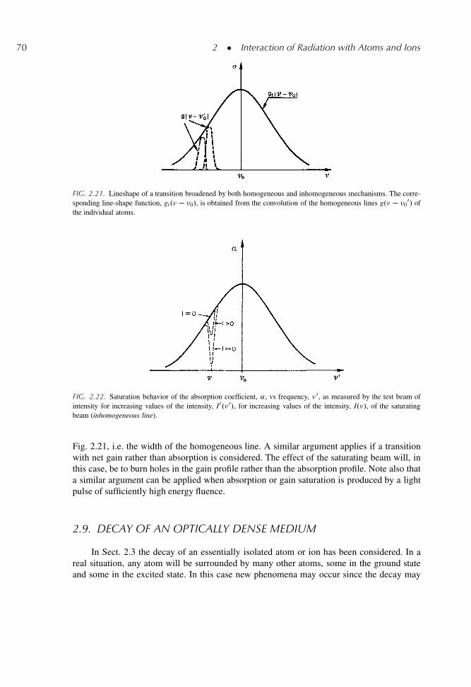
70 2 � Interaction of Radiation with Atoms and Ions
FIG. 2.21. Lineshape of a transition broadened by both homogeneous and inhomogeneous mechanisms. The corre-sponding line-shape function, gt.� � �0/, is obtained from the convolution of the homogeneous lines g.� � �0
0/ ofthe individual atoms.
FIG. 2.22. Saturation behavior of the absorption coefficient, ˛, vs frequency, �0, as measured by the test beam ofintensity for increasing values of the intensity, I0.�0/, for increasing values of the intensity, I.�/, of the saturatingbeam (inhomogeneous line).
Fig. 2.21, i.e. the width of the homogeneous line. A similar argument applies if a transitionwith net gain rather than absorption is considered. The effect of the saturating beam will, inthis case, be to burn holes in the gain profile rather than the absorption profile. Note also thata similar argument can be applied when absorption or gain saturation is produced by a lightpulse of sufficiently high energy fluence.
2.9. DECAY OF AN OPTICALLY DENSE MEDIUM
In Sect. 2.3 the decay of an essentially isolated atom or ion has been considered. In areal situation, any atom will be surrounded by many other atoms, some in the ground stateand some in the excited state. In this case new phenomena may occur since the decay may
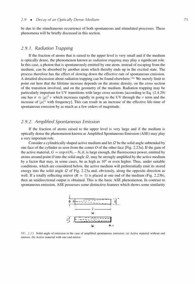
2.9 � Decay of an Optically Dense Medium 71
be due to the simultaneous occurrence of both spontaneous and stimulated processes. Thesephenomena will be briefly discussed in this section.
2.9.1. Radiation Trapping
If the fraction of atoms that is raised to the upper level is very small and if the mediumis optically dense, the phenomenon known as radiation trapping may play a significant role.In this case, a photon that is spontaneously emitted by one atom, instead of escaping from themedium, can be absorbed by another atom which thereby ends up in the excited state. Theprocess therefore has the effect of slowing down the effective rate of spontaneous emission.A detailed discussion about radiation trapping can be found elsewhere..16/ We merely limit topoint out here that the lifetime increase depends on the atomic density, on the cross sectionof the transition involved, and on the geometry of the medium. Radiation trapping may beparticularly important for UV transitions with large cross sections [according to Eq. (2.4.29)one has � / j�j2 � which increases rapidly in going to the UV through the � term and theincrease of j�j2 with frequency]. This can result in an increase of the effective life-time ofspontaneous emission by as much as a few orders of magnitude.
2.9.2. Amplified Spontaneous Emission
If the fraction of atoms raised to the upper level is very large and if the medium isoptically dense the phenomenon known as Amplified Spontaneous Emission (ASE) may playa very important role.
Consider a cylindrically shaped active medium and let˝ be the solid angle subtended byone face of the cylinder as seen from the center O of the other face [Fig. 2.23a]. If the gain ofthe active material, G D exp �.N2 � N1/l, is large enough, the fluorescence power, emitted byatoms around point O into the solid angle˝ , may be strongly amplified by the active mediumby a factor that may, in some cases, be as high as 104 or even higher. Thus, under suitableconditions, which are considered below, the active medium will preferentially emit its storedenergy into the solid angle ˝ of Fig. 2.23a and, obviously, along the opposite direction aswell. If a totally reflecting mirror .R D 1/ is placed at one end of the medium (Fig. 2.23b),then an unidirectional output is obtained. This is the basic ASE phenomenon. In contrast tospontaneous emission, ASE possesses some distinctive features which shows some similarity
FIG. 2.23. Solid angle of emission in the case of amplified spontaneous emission: (a) Active material without endmirrors. (b) Active material with one end mirror.
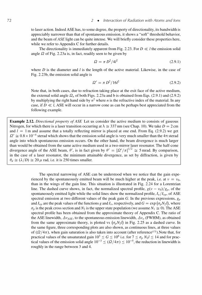
72 2 � Interaction of Radiation with Atoms and Ions
to laser action. Indeed ASE has, to some degree, the property of directionality, its bandwidth isappreciably narrower than that of spontaneous emission, it shows a “soft” threshold behavior,and the beam of ASE light can be quite intense. We will briefly consider these properties here,while we refer to Appendix C for further details.
The directionality is immediately apparent from Fig. 2.23. For D � l the emission solidangle ˝ of Fig. 2.23a is, in fact, readily seen to be given by
˝ D D2=4l2 (2.9.1)
where D is the diameter and l is the length of the active material. Likewise, in the case ofFig. 2.23b, the emission solid angle is
˝ 0 D D2=16l2 (2.9.2)
Note that, in both cases, due to refraction taking place at the exit face of the active medium,the external solid angle˝n of both Figs. 2.23a and b is obtained from Eqs. (2.9.1) and (2.9.2)by multiplying the right hand side by n2 where n is the refractive index of the material. In anycase, if D � l, ASE will occur in a narrow cone as can be perhaps best appreciated from thefollowing example.
Example 2.12. Directional property of ASE Let us consider the active medium to consists of gaseousNitrogen, for which there is a laser transition occurring at λ Š 337 nm (see Chap. 10). We take D D 2 cmand l D 1 m and assume that a totally reflecting mirror is placed at one end. From Eq. (2.9.2) we get˝ 0 Š 0.8�10�4 sterad which shows that the emission solid angle is very much smaller than the 4π steradangle into which spontaneous emission occurs. On the other hand, the beam divergence is much largerthan would be obtained from the same active medium used in a two-mirror laser resonator. The half-conedivergence angle of the ASE beam, 0, is in fact given by 0 D Œ˝ 0= �1=2 Š 5 mrad. By comparison,in the case of a laser resonator, the minimum attainable divergence, as set by diffraction, is given byd Š .�=D/ Š 20� rad, i.e. it is 250 times smaller.
The spectral narrowing of ASE can be understood when we notice that the gain expe-rienced by the spontaneously emitted beam will be much higher at the peak, i.e. at � D �0,than in the wings of the gain line. This situation is illustrated in Fig. 2.24 for a Lorentzianline. The dashed curve shows, in fact, the normalized spectral profile, g.� � �0/=gp, of thespontaneously emitted light while the solid lines show the normalized profile, I�=I�p, of ASEspectral emission at two different values of the peak gain G. In the previous expressions, gp
and I�p are the peak values of the functions g and I� , respectively, and G D exp�pN2l
�, where
�p is the peak cross section and N2 is the upper state population (we assume N1 Š 0). The ASEspectral profile has been obtained from the approximate theory of Appendix C. The ratio ofthe ASE linewidth,�ASE, to the spontaneous emission linewidth,�o (FWHM), as obtainedfrom the same approximate theory, is plotted vs
�pN2l
�in Fig. 2.25 as a dashed curve. In
the same figure, three corresponding plots are also shown, as continuous lines, at three valuesof .˝=4 /, when gain saturation is also taken into account (after reference.17/).Note that, forpractical values of the unsaturated gain 103 G 106 i.e. for 7 �p N2l 14 and for prac-tical values of the emission solid angle 10�3 .˝=4 / 10�5, the reduction in linewidth isroughly in the range between 3 and 4.
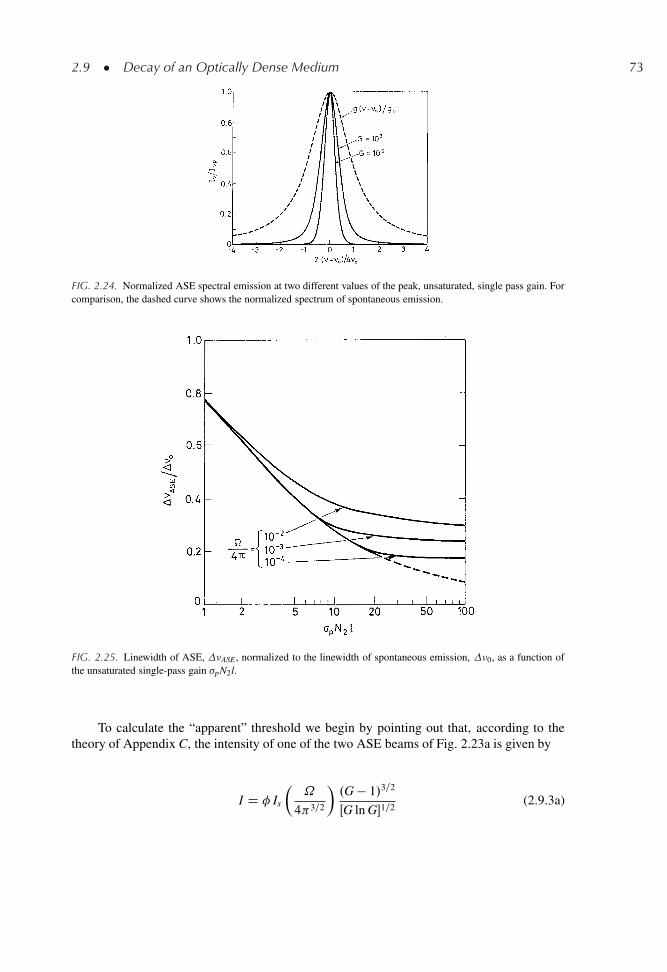
2.9 � Decay of an Optically Dense Medium 73
FIG. 2.24. Normalized ASE spectral emission at two different values of the peak, unsaturated, single pass gain. Forcomparison, the dashed curve shows the normalized spectrum of spontaneous emission.
FIG. 2.25. Linewidth of ASE, �ASE, normalized to the linewidth of spontaneous emission, �0, as a function ofthe unsaturated single-pass gain �pN2l.
To calculate the “apparent” threshold we begin by pointing out that, according to thetheory of Appendix C, the intensity of one of the two ASE beams of Fig. 2.23a is given by
I D � Is
�˝
4 3=2
�.G � 1/3=2
ŒG ln G�1=2(2.9.3a)
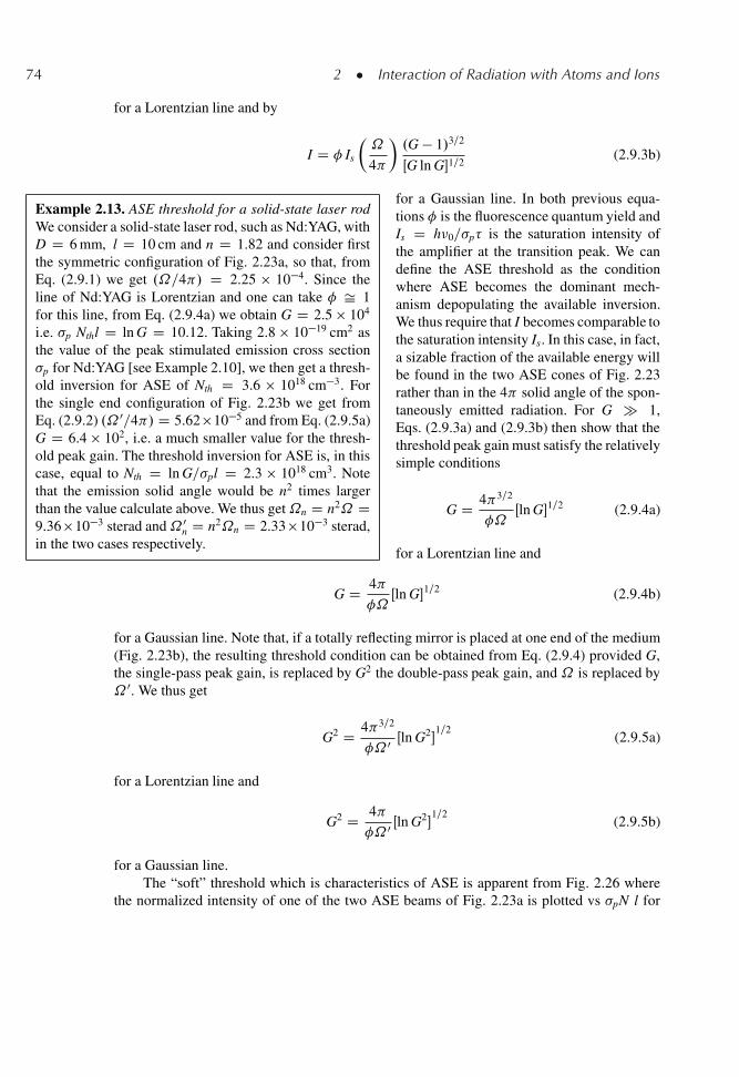
74 2 � Interaction of Radiation with Atoms and Ions
for a Lorentzian line and by
I D � Is
�˝
4
�.G � 1/3=2
ŒG ln G�1=2(2.9.3b)
Example 2.13. ASE threshold for a solid-state laser rodWe consider a solid-state laser rod, such as Nd:YAG, withD D 6 mm, l D 10 cm and n D 1.82 and consider firstthe symmetric configuration of Fig. 2.23a, so that, fromEq. (2.9.1) we get .˝=4 / D 2.25 � 10�4. Since theline of Nd:YAG is Lorentzian and one can take � Š 1for this line, from Eq. (2.9.4a) we obtain G D 2.5 � 104
i.e. �p Nthl D ln G D 10.12. Taking 2.8 � 10�19 cm2 asthe value of the peak stimulated emission cross section�p for Nd:YAG [see Example 2.10], we then get a thresh-old inversion for ASE of Nth D 3.6 � 1018 cm�3. Forthe single end configuration of Fig. 2.23b we get fromEq. (2.9.2) .˝ 0=4 / D 5.62�10�5 and from Eq. (2.9.5a)G D 6.4 � 102, i.e. a much smaller value for the thresh-old peak gain. The threshold inversion for ASE is, in thiscase, equal to Nth D ln G=�pl D 2.3 � 1018 cm3. Notethat the emission solid angle would be n2 times largerthan the value calculate above. We thus get˝n D n2˝ D9.36�10�3 sterad and˝ 0
n D n2˝n D 2.33�10�3 sterad,in the two cases respectively.
for a Gaussian line. In both previous equa-tions � is the fluorescence quantum yield andIs D h�0=�p� is the saturation intensity ofthe amplifier at the transition peak. We candefine the ASE threshold as the conditionwhere ASE becomes the dominant mech-anism depopulating the available inversion.We thus require that I becomes comparable tothe saturation intensity Is. In this case, in fact,a sizable fraction of the available energy willbe found in the two ASE cones of Fig. 2.23rather than in the 4 solid angle of the spon-taneously emitted radiation. For G � 1,Eqs. (2.9.3a) and (2.9.3b) then show that thethreshold peak gain must satisfy the relativelysimple conditions
G D 4 3=2
�˝Œln G�1=2 (2.9.4a)
for a Lorentzian line and
G D 4
�˝Œln G�1=2 (2.9.4b)
for a Gaussian line. Note that, if a totally reflecting mirror is placed at one end of the medium(Fig. 2.23b), the resulting threshold condition can be obtained from Eq. (2.9.4) provided G,the single-pass peak gain, is replaced by G2 the double-pass peak gain, and ˝ is replaced by˝ 0. We thus get
G2 D 4 3=2
�˝ 0 Œln G2�1=2
(2.9.5a)
for a Lorentzian line and
G2 D 4
�˝ 0 Œln G2�1=2
(2.9.5b)
for a Gaussian line.The “soft” threshold which is characteristics of ASE is apparent from Fig. 2.26 where
the normalized intensity of one of the two ASE beams of Fig. 2.23a is plotted vs �pN l for
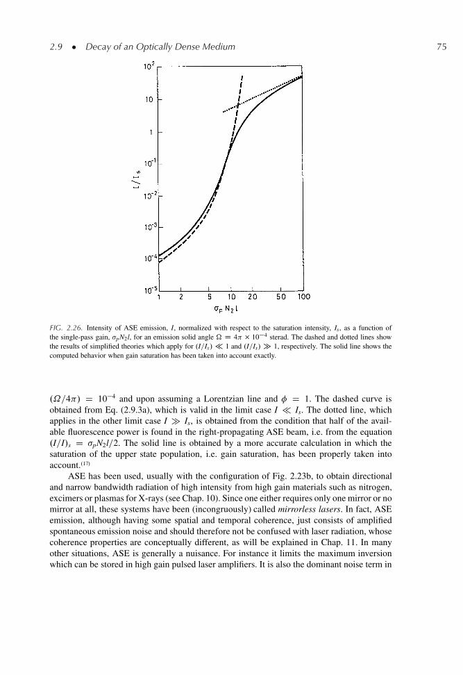
2.9 � Decay of an Optically Dense Medium 75
FIG. 2.26. Intensity of ASE emission, I, normalized with respect to the saturation intensity, Is, as a function ofthe single-pass gain, �pN2l, for an emission solid angle � D 4 10�4 sterad. The dashed and dotted lines showthe results of simplified theories which apply for .I=Is/ 1 and .I=Is/ � 1, respectively. The solid line shows thecomputed behavior when gain saturation has been taken into account exactly.
.˝=4 / D 10�4 and upon assuming a Lorentzian line and � D 1. The dashed curve isobtained from Eq. (2.9.3a), which is valid in the limit case I � Is. The dotted line, whichapplies in the other limit case I � Is, is obtained from the condition that half of the avail-able fluorescence power is found in the right-propagating ASE beam, i.e. from the equation.I=I/s D �pN2l=2. The solid line is obtained by a more accurate calculation in which thesaturation of the upper state population, i.e. gain saturation, has been properly taken intoaccount..17/
ASE has been used, usually with the configuration of Fig. 2.23b, to obtain directionaland narrow bandwidth radiation of high intensity from high gain materials such as nitrogen,excimers or plasmas for X-rays (see Chap. 10). Since one either requires only one mirror or nomirror at all, these systems have been (incongruously) called mirrorless lasers. In fact, ASEemission, although having some spatial and temporal coherence, just consists of amplifiedspontaneous emission noise and should therefore not be confused with laser radiation, whosecoherence properties are conceptually different, as will be explained in Chap. 11. In manyother situations, ASE is generally a nuisance. For instance it limits the maximum inversionwhich can be stored in high gain pulsed laser amplifiers. It is also the dominant noise term in
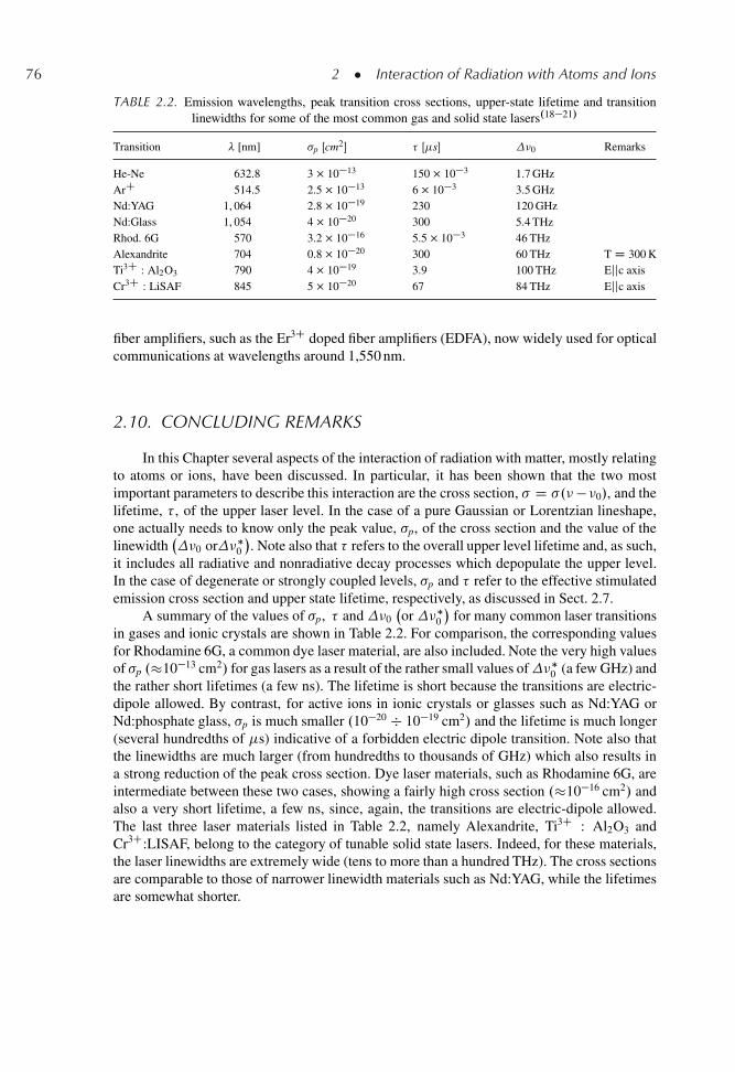
76 2 � Interaction of Radiation with Atoms and Ions
TABLE 2.2. Emission wavelengths, peak transition cross sections, upper-state lifetime and transitionlinewidths for some of the most common gas and solid state lasers.18�21/
Transition � [nm] �p Œcm2� � Œ�s� �0 Remarks
He-Ne 632.8 3 10�13 150 10�3 1.7 GHzArC 514.5 2.5 10�13 6 10�3 3.5 GHzNd:YAG 1, 064 2.8 10�19 230 120 GHzNd:Glass 1, 054 4 10�20 300 5.4 THzRhod. 6G 570 3.2 10�16 5.5 10�3 46 THzAlexandrite 704 0.8 10�20 300 60 THz T D 300 KTi3C : Al2O3 790 4 10�19 3.9 100 THz Ejjc axisCr3C : LiSAF 845 5 10�20 67 84 THz Ejjc axis
fiber amplifiers, such as the Er3C doped fiber amplifiers (EDFA), now widely used for opticalcommunications at wavelengths around 1,550 nm.
2.10. CONCLUDING REMARKS
In this Chapter several aspects of the interaction of radiation with matter, mostly relatingto atoms or ions, have been discussed. In particular, it has been shown that the two mostimportant parameters to describe this interaction are the cross section, � D �.���0/, and thelifetime, � , of the upper laser level. In the case of a pure Gaussian or Lorentzian lineshape,one actually needs to know only the peak value, �p, of the cross section and the value of thelinewidth
�0 or��
0
�. Note also that � refers to the overall upper level lifetime and, as such,
it includes all radiative and nonradiative decay processes which depopulate the upper level.In the case of degenerate or strongly coupled levels, �p and � refer to the effective stimulatedemission cross section and upper state lifetime, respectively, as discussed in Sect. 2.7.
A summary of the values of �p, � and�0or ��
0
�for many common laser transitions
in gases and ionic crystals are shown in Table 2.2. For comparison, the corresponding valuesfor Rhodamine 6G, a common dye laser material, are also included. Note the very high valuesof �p .�10�13 cm2/ for gas lasers as a result of the rather small values of��
0 (a few GHz) andthe rather short lifetimes (a few ns). The lifetime is short because the transitions are electric-dipole allowed. By contrast, for active ions in ionic crystals or glasses such as Nd:YAG orNd:phosphate glass, �p is much smaller .10�20 � 10�19 cm2/ and the lifetime is much longer(several hundredths of �s) indicative of a forbidden electric dipole transition. Note also thatthe linewidths are much larger (from hundredths to thousands of GHz) which also results ina strong reduction of the peak cross section. Dye laser materials, such as Rhodamine 6G, areintermediate between these two cases, showing a fairly high cross section .�10�16 cm2/ andalso a very short lifetime, a few ns, since, again, the transitions are electric-dipole allowed.The last three laser materials listed in Table 2.2, namely Alexandrite, Ti3C : Al2O3 andCr3C:LISAF, belong to the category of tunable solid state lasers. Indeed, for these materials,the laser linewidths are extremely wide (tens to more than a hundred THz). The cross sectionsare comparable to those of narrower linewidth materials such as Nd:YAG, while the lifetimesare somewhat shorter.
Problems 77
PROBLEMS
2.1. For a cavity volume V D 1 cm3 calculate the number of modes that fall within a bandwidth� D 10 nm centered at � D 600 nm.
2.2. Instead of �� , a spectral energy density �� can be defined, �� being such that ��d� gives theenergy density for the e.m. waves of wavelength lying between � and �Cd�. Find the relationshipbetween �� and �� .
2.3. For blackbody radiation find the maximum of �� vs �. Show in this way that the wavelength �M
at which the maximum occurs satisfies the relationship �MT D hc=ky (Wien’s law), where thequantity y satisfies the equation 5 Œ1 � exp.�y/� D y. From this equation find an approximatevalue of y.
2.4. The wavelength �M at which the maximum occurs for the distribution in Fig. 2.3 satisfies therelation �MT D 2.9�10�3 m�K (Wien’s law). Calculate �M for T D 6, 000 K. What is the colorcorresponding to this wavelength?
2.5. The R1 laser transition of ruby has, to a good approximation, a Lorentzian shape of width(FWHM) 330 GHz at room temperature (see Fig. 2.10). The measured peak transition crosssection in � D 2.5�10�20 cm2. Calculate the radiative lifetime (the refractive index is n D 1.76).Since the observed room temperature lifetime is 3 ms, what is the fluorescence quantum yield?
2.6. Nd:YAG, a typical active laser material, is a crystal of Y3Al5O12 (yttrium aluminum garnet, YAG)in which some of the Y3C ions are substituted by Nd3C ions. The typical Nd3C atomic concen-tration used is 1%, i.e. 1% of Y3C ions are replaced by Nd3C. The YAG density is 4.56 g=cm3.Calculate the Nd3C concentration in the ground .4I9=2/ level. This level is actually made up offive (doubly degenerate) levels (see Fig. 2.16), the four higher levels being spaced from the low-est level by 134, 197, 311,and 848 cm�1, respectively. Calculate the Nd3C concentration in thelowest level of the 4I9=2 state.
2.7. The neon laser transition at � D 1.15�m is predominantly Doppler broadened to �0� D 9 �
108 Hz. The upper state lifetime is �10�7 s. Calculate the peak cross section assuming that thelaser transition lifetime is equal to the total upper state lifetime.
2.8. The quantum yield of the S1 ! S0 transition (see Chap.9) for Rhodamine 6G is 0.87, and thecorresponding lifetime is �5 ns. Calculate the radiative and nonradiative lifetimes of the S1 level.
2.9. Calculate the total homogeneous linewidth of the 633 nm laser transition of Ne knowing that�nat Š 20 MHz and �c D 0.64 MHz. What is the shape of the overall line?
2.10. Find the relationship between the intensity, I, and the corresponding energy density, �, for aplane wave.
2.11. A cylindrical rod of Nd:YAG with diameter of 6.3 mm and length of 7.5 cm is pumped very hardby a suitable flashlamp. The peak cross section for the 1.06�m laser transition is � D 2.8 �10�19 cm2 and the refractive index of YAG is n D 1.82. Calculate the critical inversion for theonset of the amplified spontaneous emission (ASE) process (the two rod end faces are assumedto be perfectly antireflection coated, i.e., non-reflecting). Also calculate the maximum energy thatcan be stored in the rod if the ASE process is to be avoided.
2.12. A solution of cryptocyanine (1,10-diethyl-4,40-carbocyanine iodiode) in methanol has been usedsimultaneously to Q-switch and mode-lock (see Chap. 8) a ruby laser. The absorption cross sectionof cryptocyanine for ruby laser radiation .� D 694.3 nm/ is 8.1 � 10�16 cm2. The upper statelifetime is � Š 22 ps. Calculate the saturation intensity at this wavelength.
78 2 � Interaction of Radiation with Atoms and Ions
2.13. Upon applying the principle of detailed balance to the two near-resonant transfer processes ofEqs. (2.6.9) and (2.6.10), show that, at exact resonance i.e., for E D 0, one has kB�A D kBA� ,where kB�A and kBA� are the rate constant of the two processes, respectively
2.14. Instead of observing saturation as in Fig. 2.19, we can also do this by using just the beam I.�/ andmeasuring the absorption coefficient for this beam at sufficiently high values of the intensity I.�/.For a homogeneous line, show that the absorption coefficient is, in this case,
˛.� � �0/ D ˛0.0/
1 C Œ2.� � �0/=�0�2 C .I=Is0/
where ˛0.0/ is the unsaturated .I � Is0/ absorption coefficient at � D �0 and Is0 is the saturationintensity, as defined by Eq. (2.8.11), at � D �0. Hint: begin by showing that
˛.� � �0/ D ˛0.0/
1 C Œ2.� � �0/=�0�2
1
1 C .I=Is/
where Is is the saturation intensity at frequency �. Continue by expressing Is in terms of Is0.
2.15. From the expression derived above, find the behavior of the peak absorption coefficient and thelinewidth versus I. How would you then measure the saturation intensity Is0?
2.16. Show that, for an inhomogeneous line with line shape function g, the saturated absorptioncoefficient for an experiment as in Fig. 2.20 can be written as
˛ D
2 2
3n"0c0h
!j�j2Nt
Z.2= �0/ �
0g �00 � �0
�1 C �
2�0 � �0
0
�=�0
2 1
1 C IIs0
1
1CŒ2.���00/=��0�
2
d�00
where the homogeneous contribution is accounted for by a Lorentzian line. [Hint: begin by cal-culating the elemental contribution, d˛, of the saturated absorption coefficient due to the fractiong�.�0
0 � �0/d�00 of atoms whose resonant frequencies lie between �0
0 and �00 C d�0
0]
2.17. Under the assumptions that (1) the homogeneous linewidth is much smaller than the inhomoge-neous linewidth and (2) I � Is0, show that the expression for ˛ given in the previous problem canbe approximated as
˛ D
2 2
3n"0c0h
!j�j2Nt�
0g .�0 � �0/ �
�241 � .2= �0/
I
Is0
Zd�0
0n1 C �
2�0 � �0
0
�=�0
2o n1 C �2� � �0
0
�=�0
2o35
Since the integral is now the convolution of two Lorentzian lines, what is the width of the hole inFig. 2.22?
References
1. R. Reiff, Fundamentals of Statistical and Thermal Physics, (McGraw-Hill, New York, 1965), Chap. 92. W. Heitler, The Quantum Theory of Radiation, 3rd edn.(Oxford University Press, London, 1953), Sect. II.93. J.A. Stratton, Electromagnetic Theory, 1st edn. (McGraw-Hill, New York, 1941), pp. 431–4384. R.H. Pantell and H.E. Puthoff, Fundamentals of Quantum Electronics, (Wiley, New York, 1964), Chap. 6
References 79
5. W. Louisell, Radiation and Noise in Quantum Electronics, (McGraw-Hill, New York, 1964), Chap. 66. H.A. Lorentz, The Theory of Electrons, 2nd edn. (Dover, New York 1952), Chap. III7. A. Einstein, On the Quantum Theory of Radiation, Z. Phys. 18, 121 (1917)8. Radiation and Noise in Quantum Electronics, (McGraw-Hill, New York, 1964), Chap. 59. H.G. Kuhn, Atomic Spectra, 2nd edn. (Longmans, Green, London 1969), Chap. VII
10. Radiationless Transitions, ed. by F.J. Fong (Springer-Verlag, Berlin, 1976) Chap. 411. C.K. Rhodes and A. Szoke, Gaseous Lasers: Atomic, Molecular, Ionic in Laser Handbook ed. by F.T. Arecchi
and E.O. Schultz-DuBois (North Holland, Amsterdam 1972) Vol. 1 pp 265–32412. J.B. Birks, Photophysics of Aromatic Molecules (Wiley-Interscience, New-York, 1970), Sect. 11.913. D.L. Dexter, J. Chem. Phys. 21, 836 (1953)14. J.D. Jackson, Classical Electrodynamics (Wiley, New York, 1975) Sect. 9.215. W.J. Miniscalco, Optical and Electronic Properties of Rare Earth Ions in Glasses, in Rare Earth Doped Fiber
Lasers and Amplifiers ed. by M.J.F. Digonnet (Marcel Dekker, New York, 1993), Chap. 216. T. Holstein, Imprisonment of Resonant Radiation in Gases, Phys. Rev. 72, 1212 (1947)17. L.W. Casperson, Threshold Characteristics of Mirrorless Lasers, J. Appl. Phys. 48, 256 (1977)18. R. Arrathoon, Helium-Neon Lasers and the Positive Column in Lasers ed. by A.K. Levine and A.J. DeMaria
(Marcel Dekker, New York, 1976), Tab. 219. M.H. Dunn and J.N. Ross, The Argon Laser in Progress in Quantum Electronics, Vol. 4 ed. by J.H. Sanders and
S. Stenholm (Pergamon Press, Oxford 1977), Tab. 220. W.F. Krupke, M.D. Shinn, J.E. Marion, J.A. Caird, S.E. Stokowski, Spectroscopic, Optical, and Thermomechan-
ical Properties of Neodymium- and Chromium-Doped Gadolinium Scandium Gallium Garnet, J. Opt. Soc. Am.B 3, 102 (1986)
21. J.C. Walling, O.G. Peterson, J.P. Jennsen, R.C. Morris, and E.W. O’Dell, Tunable Alexandrite Lasers, IEEE J.Quant. Electr. QE-16, 1302 (1980)
3
Energy Levels, Radiativeand Nonradiative Transitionsin Molecules and Semiconductors
The purpose of this chapter is to specialize some of the results and considerations of theprevious chapter to the somewhat more complicated case of molecules and semiconductors.Particular emphasis will be given to semiconductors, either in bulk or quantum well form,since they play an increasingly important role as laser media.
3.1. MOLECULES
We will first consider the energy levels, and the radiative and nonradiative transitionsin molecules. The considerations will be limited to a qualitative description of those featureswhich are particularly relevant for a correct understanding of laser action in active media suchas molecular gases or organic dyes. For a more extensive treatment of the wider subject ofmolecular physics the reader is referred to specialized texts..1/
3.1.1. Energy Levels
The total energy of a molecule consists generally of the sum of four contributions: (1)electronic energy, Ee due to the motion of electrons about the nuclei; (2) vibrational energyEv, due to the vibrational motion of the nuclei; (3) rotational energy Er, due to the rotationalmotion of the molecule; and (4) translational energy. We will not consider the translationalenergy any further since it is not usually quantized. The other types of energy, however, arequantized and it is instructive to derive, from simple arguments, the order of magnitude of the
O. Svelto, Principles of Lasers,c
81DOI: 10.1007/978-1-4419-1302-9 3, � Springer Science+Business Media LLC 2010
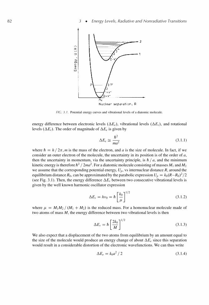
82 3 � Energy Levels, Radiative and Nonradiative Transitions
FIG. 3.1. Potential energy curves and vibrational levels of a diatomic molecule.
energy difference between electronic levels .�Ee/, vibrational levels .�Ev/, and rotationallevels .�Er/. The order of magnitude of �Ee is given by
�Ee Š „2
ma2(3.1.1)
where „ D h = 2 , m is the mass of the electron, and a is the size of molecule. In fact, if weconsider an outer electron of the molecule, the uncertainty in its position is of the order of a,then the uncertainty in momentum, via the uncertainty principle, is „ = a, and the minimumkinetic energy is therefore „2 = 2ma2. For a diatomic molecule consisting of masses M1 and M2
we assume that the corresponding potential energy, Up, vs internuclear distance R, around theequilibrium distance R0, can be approximated by the parabolic expression Up D k0.R�R0/
2=2(see Fig. 3.1). Then, the energy difference�Ev between two consecutive vibrational levels isgiven by the well known harmonic oscillator expression
�Ev D h�0 D „�
k0
�
�1=2
(3.1.2)
where � D M1M2 = .M1 C M2/ is the reduced mass. For a homonuclear molecule made oftwo atoms of mass M, the energy difference between two vibrational levels is then
�Ev D „�
2k0
M
�1=2
(3.1.3)
We also expect that a displacement of the two atoms from equilibrium by an amount equal tothe size of the molecule would produce an energy change of about �Ee since this separationwould result in a considerable distortion of the electronic wavefunctions. We can thus write
�Ee D k0a2 = 2 (3.1.4)
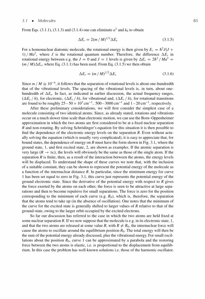
3.1 � Molecules 83
From Eqs. (3.1.1), (3.1.3) and (3.1.4) one can eliminate a2 and k0 to obtain
�Ev D 2.m =M/1=2�Ee (3.1.5)
For a homonuclear diatomic molecule, the rotational energy is then given by Er D „2J.J C1/ =Ma2, where J is the rotational quantum number. Therefore, the difference �Er inrotational energy between e.g. the J D 0 and J D 1 levels is given by �Er D 2„2 =Ma2 D.m =M/�Ee, where Eq. (3.1.1) has been used. From Eq. (3.1.5) we then obtain
�Er D .m =M/1=2�Ev (3.1.6)
Since m =M Š 10�4, it follows that the separation of rotational levels is about one-hundredththat of the vibrational levels. The spacing of the vibrational levels is, in turn, about one-hundredth of �Ee. In fact, as indicated in earlier discussion, the actual frequency ranges,.�Ee = h/, for electronic, .�Ev = h/, for vibrational and, .�Er = h/, for rotational transitionsare found to be roughly 25 – 50 � 103 cm�1, 500 – 3000 cm�1 and 1 – 20 cm�1, respectively.
After these preliminary considerations, we will first consider the simplest case of amolecule consisting of two identical atoms. Since, as already stated, rotations and vibrationsoccur on a much slower time scale than electronic motion, we can use the Born–Oppenheimerapproximation in which the two atoms are first considered to be at a fixed nuclear separationR and non-rotating. By solving Schrodinger’s equation for this situation it is then possible tofind the dependence of the electronic energy levels on the separation R. Even without actu-ally solving the equation (which is usually very complicated), it is easy to appreciate that, forbound states, the dependence of energy on R must have the form shown in Fig. 3.1, where theground state, 1, and first excited state, 2, are shown as examples. If the atomic separation isvery large .R ! 1/, the levels will obviously be the same as those of the single atom. If theseparation R is finite, then, as a result of the interaction between the atoms, the energy levelswill be displaced. To understand the shape of these curves we note that, with the inclusionof a suitable constant, they can be shown to represent the potential energy of the molecule asa function of the internuclear distance R. In particular, since the minimum energy for curve1 has been set equal to zero in Fig. 3.1, this curve just represents the potential energy of theground electronic state. Since the derivative of the potential energy with respect to R givesthe force exerted by the atoms on each other, the force is seen to be attractive at large sepa-rations and then to become repulsive for small separations. The force is zero for the positioncorresponding to the minimum of each curve (e.g. R0), which is, therefore, the separationthat the atoms tend to take up (in the absence of oscillation). One notes that the minimum ofthe curve for the excited state is generally shifted to larger values of R relative to that of theground-state, owing to the larger orbit occupied by the excited electrons.
So far our discussion has referred to the case in which the two atoms are held fixed atsome nuclear separation R. If we now suppose that the molecule is e.g. in its electronic state, 1,and that the two atoms are released at some value R, with R ¤ R0, the internuclear force willcause the atoms to oscillate around the equilibrium position R0. The total energy will then bethe sum of the potential energy already discussed, plus the vibrational energy. For small oscil-lations about the position R0, curve 1 can be approximated by a parabola and the restoringforce between the two atoms is elastic, i.e. is proportional to the displacement from equilib-rium. In this case the problem has well-known solutions i.e. those of the harmonic oscillator.
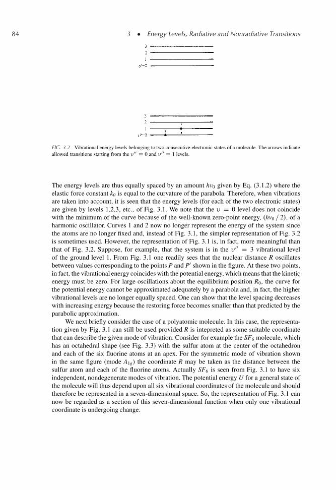
84 3 � Energy Levels, Radiative and Nonradiative Transitions
FIG. 3.2. Vibrational energy levels belonging to two consecutive electronic states of a molecule. The arrows indicateallowed transitions starting from the �00 D 0 and �00 D 1 levels.
The energy levels are thus equally spaced by an amount hv0 given by Eq. (3.1.2) where theelastic force constant k0 is equal to the curvature of the parabola. Therefore, when vibrationsare taken into account, it is seen that the energy levels (for each of the two electronic states)are given by levels 1,2,3, etc., of Fig. 3.1. We note that the � D 0 level does not coincidewith the minimum of the curve because of the well-known zero-point energy, .hv0 = 2/, of aharmonic oscillator. Curves 1 and 2 now no longer represent the energy of the system sincethe atoms are no longer fixed and, instead of Fig. 3.1, the simpler representation of Fig. 3.2is sometimes used. However, the representation of Fig. 3.1 is, in fact, more meaningful thanthat of Fig. 3.2. Suppose, for example, that the system is in the � 00 D 3 vibrational levelof the ground level 1. From Fig. 3.1 one readily sees that the nuclear distance R oscillatesbetween values corresponding to the points P and P0 shown in the figure. At these two points,in fact, the vibrational energy coincides with the potential energy, which means that the kineticenergy must be zero. For large oscillations about the equilibrium position R0, the curve forthe potential energy cannot be approximated adequately by a parabola and, in fact, the highervibrational levels are no longer equally spaced. One can show that the level spacing decreaseswith increasing energy because the restoring force becomes smaller than that predicted by theparabolic approximation.
We next briefly consider the case of a polyatomic molecule. In this case, the representa-tion given by Fig. 3.1 can still be used provided R is intepreted as some suitable coordinatethat can describe the given mode of vibration. Consider for example the SF6 molecule, whichhas an octahedral shape (see Fig. 3.3) with the sulfur atom at the center of the octahedronand each of the six fluorine atoms at an apex. For the symmetric mode of vibration shownin the same figure (mode A1g) the coordinate R may be taken as the distance between thesulfur atom and each of the fluorine atoms. Actually SF6 is seen from Fig. 3.1 to have sixindependent, nondegenerate modes of vibration. The potential energy U for a general state ofthe molecule will thus depend upon all six vibrational coordinates of the molecule and shouldtherefore be represented in a seven-dimensional space. So, the representation of Fig. 3.1 cannow be regarded as a section of this seven-dimensional function when only one vibrationalcoordinate is undergoing change.
3.1 � Molecules 85
FIG. 3.3. Normal modes of vibration of an octahedral molecule (e.g. SF6) The sulfur atom occupies the center ofthe octahedron and the six fluorine atoms are at the corners of the octahedron (after ref..2/ by permission).
The description given so far does not give a complete picture of the molecular systemsince we have ignored the fact that molecule can also rotate. According to quantum mechanicsthe rotational energy is also quantized, and, for a linear rigid rotator (e.g. a rigid diatomic orlinear triatomic molecule), it can be expressed as
Er D BJ.J C 1/ (3.1.7)
where the rotational constant B is given by „2 = 2I with I being the moment of inertia aboutan axis perpendicular to the internuclear axis and through the center of mass. Thus, the totalenergy of the system is given by the sum of the electronic, vibrational, and rotational energies.Accordingly the energy levels of, say, the � 00 D 0 and � 0 D 1 vibrational levels of the groundstate will be as indicated in Fig. 3.4. Note that, unlike tha case for vibrational levels, thespacing between consecutive rotational levels is not constant. In fact it increases linearly withthe rotational quantum number J, i.e. ŒEr.J/� Er.J � 1/� D 2BJ.
3.1.2. Level Occupation at Thermal Equilibrium
At thermodynamic equilibrium the population, N.Ee, Ev, Er/, of a rotational-vibrationallevel belonging to a given electronic state can be written as
N.Ee, Ev, Er/ / gegvgr exp � Œ.Ee C Ev C Er/ = kT� (3.1.8)
where Ee, Ev, and Er are the electronic, vibrational, and rotational energies of the level andge, gv, and gr are the corresponding level degeneracies [see Eq. (2.7.3)]. According to theestimates of the previous section, the order of magnitude of Ev = hc is 1,000 cm�1 while Ee = hc

86 3 � Energy Levels, Radiative and Nonradiative Transitions
FIG. 3.4. Rotational energy levels belonging to two consecutive vibrational states of a molecule. The arrows indicateallowed transitions belonging to the P – branch and R – branch.
is more than an order of magnitude larger. Since kT = hc Š 209 cm�1 (at T D 300 K), it thenfollows that both Ee and Ev are appreciably larger than kT. Accordingly we can say as a “ruleof thumb” that, at thermal equilibrium at room temperature, a molecule lies in the lowestvibrational level� of the ground electronic state. The probability of occupation of a givenrotational level of this lowest vibrational state can then be written, according to Eqs. (3.1.7)and (3.1.8), as
p.J/ / .2J C 1/ exp Œ�BJ.J C 1/ = kT� (3.1.9)
The factor .2J C1/ in front of the exponential accounts for level degeneracy: a rotational levelof quantum number J is in fact .2JC1/-fold degenerate. Taking, as an example, B D 0.5 cm�1
and assuming kT D 209 cm�1 (room temperature) we show in Fig. 3.5 the population distri-bution among the various rotational levels of a given vibrational state (e.g. the ground state).Note that, as a result of the factor .2J C 1/ in Eq. (3.1.9), the most heavily populated levelis not the ground (i.e. J D 0) level but rather the one whose rotational quantum number Jsatisfies the relation
.2J C 1/m D .2kT =B/1=2 (3.1.10)
A conclusion that can be drawn from this section is that for simple molecules at room tem-perature, the molecular population will be distributed among several rotational levels of theground vibrational state.
� While this statement is true for diatomic molecules, it is generally not true for polyatomic molecules. In the lattercase (e.g., the SF6 molecule) the spacing between vibrational levels is often appreciably smaller than 1000 cm�1
(down to � 100 cm�1) and many excited vibrational levels of the ground electronic state may have a significantpopulation at room temperature.
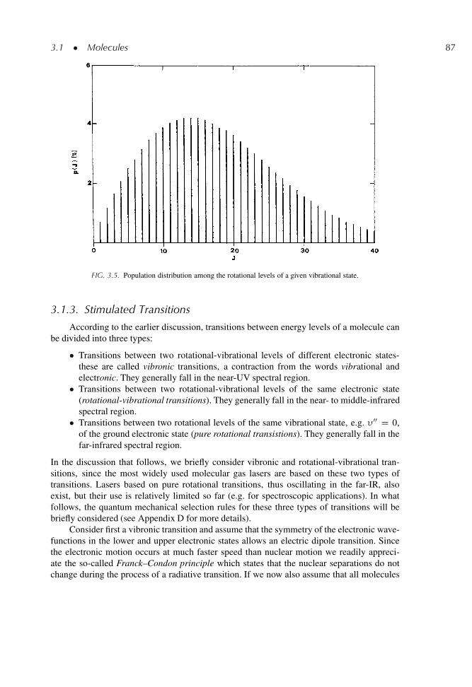
3.1 � Molecules 87
FIG. 3.5. Population distribution among the rotational levels of a given vibrational state.
3.1.3. Stimulated Transitions
According to the earlier discussion, transitions between energy levels of a molecule canbe divided into three types:
� Transitions between two rotational-vibrational levels of different electronic states-these are called vibronic transitions, a contraction from the words vibrational andelectronic. They generally fall in the near-UV spectral region.
� Transitions between two rotational-vibrational levels of the same electronic state(rotational-vibrational transitions). They generally fall in the near- to middle-infraredspectral region.
� Transitions between two rotational levels of the same vibrational state, e.g. � 00 D 0,of the ground electronic state (pure rotational transistions). They generally fall in thefar-infrared spectral region.
In the discussion that follows, we briefly consider vibronic and rotational-vibrational tran-sitions, since the most widely used molecular gas lasers are based on these two types oftransitions. Lasers based on pure rotational transitions, thus oscillating in the far-IR, alsoexist, but their use is relatively limited so far (e.g. for spectroscopic applications). In whatfollows, the quantum mechanical selection rules for these three types of transitions will bebriefly considered (see Appendix D for more details).
Consider first a vibronic transition and assume that the symmetry of the electronic wave-functions in the lower and upper electronic states allows an electric dipole transition. Sincethe electronic motion occurs at much faster speed than nuclear motion we readily appreci-ate the so-called Franck–Condon principle which states that the nuclear separations do notchange during the process of a radiative transition. If we now also assume that all molecules
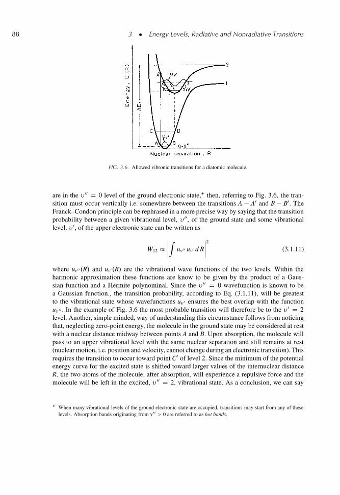
88 3 � Energy Levels, Radiative and Nonradiative Transitions
FIG. 3.6. Allowed vibronic transitions for a diatomic molecule.
are in the � 00 D 0 level of the ground electronic state,� then, referring to Fig. 3.6, the tran-sition must occur vertically i.e. somewhere between the transitions A � A0 and B � B0. TheFranck–Condon principle can be rephrased in a more precise way by saying that the transitionprobability between a given vibrational level, � 00, of the ground state and some vibrationallevel, � 0, of the upper electronic state can be written as
W12 /ˇˇZ uv00 uv0 d R
ˇˇ2 (3.1.11)
where uv00.R/ and uv0.R/ are the vibrational wave functions of the two levels. Within theharmonic approximation these functions are know to be given by the product of a Gaus-sian function and a Hermite polynominal. Since the � 00 D 0 wavefunction is known to bea Gaussian function., the transition probability, according to Eq. (3.1.11), will be greatestto the vibrational state whose wavefunctions u�0 ensures the best overlap with the functionu�00 . In the example of Fig. 3.6 the most probable transition will therefore be to the � 0 D 2level. Another, simple minded, way of understanding this circumstance follows from noticingthat, neglecting zero-point energy, the molecule in the ground state may be considered at restwith a nuclear distance midway between points A and B. Upon absorption, the molecule willpass to an upper vibrational level with the same nuclear separation and still remains at rest(nuclear motion, i.e. position and velocity, cannot change during an electronic transition). Thisrequires the transition to occur toward point C0 of level 2. Since the minimum of the potentialenergy curve for the excited state is shifted toward larger values of the internuclear distanceR, the two atoms of the molecule, after absorption, will experience a repulsive force and themolecule will be left in the excited, � 00 D 2, vibrational state. As a conclusion, we can say
� When many vibrational levels of the ground electronic state are occupied, transitions may start from any of theselevels. Absorption bands originating from v00 > 0 are referred to as hot bands.
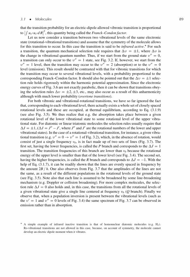
3.1 � Molecules 89
that the transition probability for an electric-dipole allowed vibronic transition is proportionaltoˇR
uv00uv0d Rˇ2
, this quantity being called the Franck–Condon factor.Let us now consider a transition between two vibrational levels of the same electronic
state (rotational-vibrational transitions) and assume that the symmetry of the molecule allowsfor this transition to occur. In this case the transition is said to be infrared active.� For sucha transition, the quantum mechanical selection rule requires that �� D ˙1, where �� isthe change in vibrational quantum number. Thus, if we start from the ground state � 00 D 0,a transition can only occur to the � 00 D 1 state, see Fig. 3.2. If, however, we start from the� 00 D 1 level, then the transition may occur to the � 00 D 2 (absorption) or to the � 00 D 0level (emission). This result should be contrasted with that for vibronic transitions for whichthe transition may occur to several vibrational levels, with a probability proportional to thecorresponding Franck–Condon factor. It should also be pointed out that the �� D ˙1 selec-tion rule holds rigorously within the harmonic potential approximation. Since the electronicenergy curves of Fig. 3.6 are not exactly parabolic, then it can be shown that transitions obey-ing the selection rules �� D ˙2, ˙3, etc., may also occur as a result of this anharmonicityalthough with much lower probability (overtone transitions).
For both vibronic and vibrational-rotational transitions, we have so far ignored the factthat, corresponding to each vibrational level, there actually exists a whole set of closely spacedrotational levels and these are occupied, at thermal equilibrium, according to Eq. (3.1.9)(see also Fig. 3.5). We thus realize that e.g. the absorption takes place between a givenrotational level of the lower vibrational state to some rotational level of the upper vibra-tional state. For diatomic or linear triatomic molecules the selection rules usually require that�J D ˙1, .�J D J00 � J0, where J00 and J0 are the rotational numbers of the lower and uppervibrational states). In the case of a rotational-vibrational transition, for instance, a given vibra-tional transition (e.g. � 00 D 0 ! � 00 D 1 of Fig. 3.2), which, in the absence of rotation, wouldconsist of just a single frequency v0, is in fact made up of two sets of lines (Fig. 3.7). Thefirst set, having the lower frequencies, is called the P branch and corresponds to the �J D 1transition. The transition frequencies of this branch are lower than v0 because the rotationalenergy of the upper level is smaller than that of the lower level (see Fig. 3.4). The second set,having the higher frequencies, is called the R branch and corresponds to �J D �1. With thehelp of Eq. (3.1.7), it can be readily shown that the lines are evenly spaced in frequency bythe amount 2B = h. One also observes from Fig. 3.7 that the amplitudes of the lines are notthe same, as a result of the different populations in the rotational levels of the ground state(see Fig. 3.5). Note also that each line is assumed to be broadened by some line-broadeningmechanism (e.g. Doppler or collision broadening). For more complex molecules, the selec-tion rule �J D 0 also holds and, in this case, the transitions from all the rotational levels ofa given vibrational state give a single line centered at frequency �0 (Q branch). Finally weobserve that, when a population inversion is present between the vibrational levels (such asthe � 0 D 1 and � 00 D 0 levels of Fig. 3.4) the same spectrum of Fig. 3.7 can be observed inemission rather than in absorption.
� A simple example of infrared inactive transition is that of homonuclear diatomic molecules (e.g. H2).Ro-vibrational transitions are not allowed in this case, because, on account of symmetry, the molecule cannotdevelop an electric dipole moment when it vibrates.
90 3 � Energy Levels, Radiative and Nonradiative Transitions
FIG. 3.7. Transitions between two vibrational levels, taking account of the rotational splitting. This transition, which,in the absence of rotational energy, would consist of a single line centered at v0, actually consists of two groups oflines: the so-called P – branch, which corresponds to a jump in rotational quantum number of �J D C1 and theso-called R – branch, which corresponds to a jump in rotational quantum number of �J D �1.
Example 3.1. Emission spectrum of the CO2 laser transition at � D 10.6�m. Here we will consider the00ı1 ! 10ı0 transition (see the section on CO2 lasers in Chap. 10), whose fundamental frequency, �0, inwavenumbers is at �0 D 960.8 cm�1..20/ The rotational constant of the CO2 molecule is B Š 0.387 cm�1.20/
and this value will be taken to be the same for upper .00ı1/ and lower .10ı0/ vibrational levels. Fromprevious considerations, the transition energies of the P-branch transitions are given by
E D h �0 C BJ0.J0 C 1/� BJ00.J00 C 1/ D h �0 � 2BJ00 (3.1.12)
where J00 is the rotational quantum number of the lower vibrational state. The rotational number J0m of
the most populated rotational level of the upper vibrational state is given by Eq. (3.1.10). Assuming arather hot CO2 molecule, i.e. T D 450 K, we get Jmax � 19.6. For the CO2 molecule, symmetry dictatesthat only J0.odd/ ! J00.even/ transitions can occur. Thus the most populated rotational level in the upperstate which is available for the transition is either the J0 D 19 or the J0 D 21 level. Assuming that theJ0 D 21 level is the most populated, this level will decay, for a P-branch transition, to the J00 D 22level [P(22) transition]. The corresponding transition frequency, according to Eq. (3.1.12), will then be� D �0 �.2BJ00=h/ D 943.8 cm�1, corresponding to a wavelength of � D .1=943.8/ cm Š 10.6�m. Notethat the wavelength corresponding to the fundamental frequency �0 is � D c=�0 Š 10.4�m. Since onlyeven J00 numbers are involved, the separation between two consecutive P-branch transitions, according toEq. (3.1.12), will given by �� D 2B�J00 D 4B D 1.55 cm�1.
Example 3.2. Doppler linewidth of a CO2 laser. Consider a CO2 laser oscillating on the P.22/ line at� D 10.6�m and assume T D 450 K [see example 3.1]. Then from Eq. (2.5.18), using the appropriatemass of CO2 we get ���
0 Š 50 MHz. Note that, since according to Eq. (2.5.18) one has ���0 / �0, the
calculated linewidth for a CO2 molecule is much smaller than that of the He-Ne laser in example 2.7 ofChap. 2, essentially because the oscillation frequency �0 is now approximately 17 times smaller. Note alsothat the gas is assumed hotter in this case because, to obtain the high output powers typical of CO2 lasers,higher pump power are used than in the He–Ne case.
3.1 � Molecules 91
Example 3.3. Collision broadening of a CO2 laser. We will consider a CO2 laser containing a gas mixtureof the H2, N2, and CO2. In this case, the laser linewidth due to collision broadening is found experi-mentally to be given by � � D 77.58 . CO2 C 0.73 N2 C 0.6 He/ � p .300=T/1=2 MHz [compare withEqs. (2.5.12) and (2.5.11)] where are the fractional partial pressures of the gas mixture, T is the gastemperature and p is the total pressure (in Torr). Taking, as an example, a typical low pressure gas mixture(p Š 15 Torr in a 1:1:8 CO2 : N2 : He mixture) at T D 450 K we get� �c Š 40 MHz. A comparison withthe result of example 3.2 then shows that, for a low pressure CO2 laser, collision broadening is compara-ble to Doppler broadening. However, for higher pressure CO2 lasers, e.g. atmospheric pressure lasers (seeChap. 10), collision broadening becomes the dominant line broadening mechanism.
Finally, for pure rotational transitions, the selection rule requires that the molecule pos-sess a permanent dipole moment. In fact, considering e.g. the phenomenon of spontaneousemission, the emitted radiation can be looked upon as originating from the rotation of thisdipole moment. For a diatomic or linear triatomic molecule the selection rule further requiresthat �J D ˙1. Thus, in the case of stimulated emission from a given rotational level J,transitions can only occur to the rotational level with quantum number J � 1.
Before continuing, it is worth summarizing the selection rules which apply for vibronic,rotational-vibrational, and rotational transitions. For an electric dipole allowed vibronic tran-sition one has �J D ˙1 for the change of rotational quantum number while the change inthe vibrational quantum number is not strictly established by a precise selection rule. In fact,starting from a given vibrational level � 00 of the lower electronic state the transition may occurto several vibrational levels of the upper electronic state with probabilities proportional to thecorresponding Franck–Condon factors. For an infrared-active rotational-vibrational transition,one must have, within the harmonic approximation, �� D ˙1 for the change of vibrationalquantum number and again�J D ˙1 for the change of rotational quantum number. For purerotational transitions in molecules with a permanent dipole moment one again has�J D ˙1.
3.1.4. Radiative and Nonradiative Decay
Let us first consider spontaneous emission and assume that the molecule is raised tosome vibrational level of an excited electronic state (Fig. 3.6). From this state the moleculeoften decays rapidly by some nonradiative process (e.g. by collision) to the � 0 D 0 vibra-tional level.� This is particularly the case for molecules in the liquid phase where collisionsoccur very frequently. From there the molecule may decay radiatively to a vibrational levelof the ground state (fluorescence see Fig. 3.6). This transition again occurs vertically and thetransition probability from the � 0 D 0 level to some level of the ground state will again beproportional to the corresponding Franck–Condon factor. Again roughly speaking, the groundstate vibrational levels involved will be those nearby the CD level of Fig. 3.6. Finally, by non-radiative decay (e.g. by collisions), the molecule rapidly returns to the � 00 D 0 level of theground electronic state (or, more precisely, thermal equilibrium is again established in theground electronic state). It is now clear from Fig. 3.6 why the fluorescence wavelength is
� Actually, this rapid decay results in a thermalization of the molecules in the upper electronic state. The probabilityof occupation of a given vibrational level of this state is thus given by (3.2.8). For simple molecules, therefore, thelowest vibrational level has the predominant populatation.
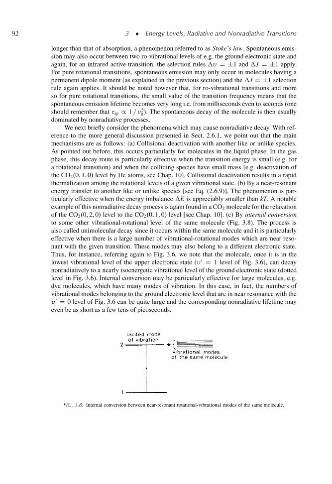
92 3 � Energy Levels, Radiative and Nonradiative Transitions
longer than that of absorption, a phenomenon referred to as Stoke’s law. Spontaneous emis-sion may also occur between two ro-vibrational levels of e.g. the ground electronic state andagain, for an infrared active transition, the selection rules �� D ˙1 and �J D ˙1 apply.For pure rotational transitions, spontaneous emission may only occur in molecules having apermanent dipole moment (as explained in the previous section) and the �J D ˙1 selectionrule again applies. It should be noted however that, for ro-vibrational transitions and moreso for pure rotational transitions, the small value of the transition frequency means that thespontaneous emission lifetime becomes very long i.e. from milliseconds even to seconds (oneshould remember that �sp / 1 = �3
0). The spontaneous decay of the molecule is then usuallydominated by nonradiative processes.
We next briefly consider the phenomena which may cause nonradiative decay. With ref-erence to the more general discussion presented in Sect. 2.6.1, we point out that the mainmechanisms are as follows: (a) Collisional deactivation with another like or unlike species.As pointed out before, this occurs particularly for molecules in the liquid phase. In the gasphase, this decay route is particularly effective when the transition energy is small (e.g. fora rotational transition) and when the colliding species have small mass [e.g. deactivation ofthe CO2.0, 1, 0/ level by He atoms, see Chap. 10]. Collisional deactivation results in a rapidthermalization among the rotational levels of a given vibrational state. (b) By a near-resonantenergy transfer to another like or unlike species [see Eq. (2.6.9)]. The phenomenon is par-ticularly effective when the energy imbalance �E is appreciably smaller than kT. A notableexample of this nonradiative decay process is again found in a CO2 molecule for the relaxationof the CO2.0, 2, 0/ level to the CO2.0, 1, 0/ level [see Chap. 10]. (c) By internal conversionto some other vibrational-rotational level of the same molecule (Fig. 3.8). The process isalso called unimolecular decay since it occurs within the same molecule and it is particularlyeffective when there is a large number of vibrational-rotational modes which are near reso-nant with the given transition. These modes may also belong to a different electronic state.Thus, for instance, referring again to Fig. 3.6, we note that the molecule, once it is in thelowest vibrational level of the upper electronic state (� 0 D 1 level of Fig. 3.6), can decaynonradiatively to a nearly isoenergetic vibrational level of the ground electronic state (dottedlevel in Fig. 3.6). Internal conversion may be particularly effective for large molecules, e.g.dye molecules, which have many modes of vibration. In this case, in fact, the numbers ofvibrational modes belonging to the ground electronic level that are in near resonance with the� 0 D 0 level of Fig. 3.6 can be quite large and the corresponding nonradiative lifetime mayeven be as short as a few tens of picoseconds.
FIG. 3.8. Internal conversion between near-resonant rotational-vibrational modes of the same molecule.
3.2 � Bulk Semiconductors 93
3.2. BULK SEMICONDUCTORS
In this section we will consider the problem of interaction of radiation with matter inthe case of a bulk semiconductor, i.e. whose physical dimensions are much larger than thede Broglie wavelength of the electrons under consideration. The case of quantum-confinedsemiconductors [quantum wells, quantum wires and quantum dots], wherein one, two, or allthree physical dimensions, respectively, are comparable to the De Broglie wavelength andwhich play an increasingly important role in laser physics, will be considered in the next twosections. Again we will limit our description to the most prominent features of the complexphenomena that occur. For a more extensive treatment of this subject the reader is referred toa specialized text..3/
3.2.1. Electronic States
The outer electrons of the atom of a semiconductor material are delocalized over thewhole crystal and the corresponding wave functions can then be written as Bloch wavefunctions.4/
.r/ D uk.r/Œexp j.k � r/� (3.2.1)
where uk.r/ has the periodicity of the crystalline lattice. The substitution of Eq. (3.2.1) intothe Schrodinger wave equation shows that the corresponding eigenvalues of the electronenergy, E, are a function of k and that these values fall within allowed bands. From nowon we will limit our considerations to the highest filled band, known as the valence band,and the next higher one, known as the conduction band. Within the parabolic band approx-imation, the E vs k relations can be approximated by a parabola and we then arrive at thepicture of Fig. 3.9 for the valence and conduction bands. The energy Ec in the conductionband, measured from the bottom of the band upwards (Fig. 3.9a), can then be written as
Ec D „2 k2
2mc(3.2.2a)
where mc D „2=Œd2 Ec = d k2�kD0 is the effective mass of the electron at the bottom of theconduction band. Likewise, the energy in the valence band, measured from the top of theband downwards (Fig. 3.9a), can be written as
Ev D „2 k2
2mv(3.2.2b)
where mv D „2=.d2Ev = d k2/kD0 is the effective mass of the electron at the top of the valenceband. In some cases, particularly when dealing with a given transition, it may be more con-venient to refer the energy to the same reference level e.g. from the top of the valence bandupwards (Fig. 3.9b). If we call E0 the energy in this coordinate system, the energies in theconduction and valence bands are now obviously given by
E0c D Eg C Ec (3.2.3a)
E0v D �Ev (3.2.3b)
where Eg is the energy gap.
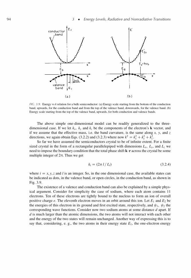
94 3 � Energy Levels, Radiative and Nonradiative Transitions
FIG. 3.9. Energy vs k relation for a bulk semiconductor: (a) Energy scale starting from the bottom of the conductionband, upwards, for the conduction band and from the top of the valence band, downwards, for the valence band. (b)Energy scale starting from the top of the valence band, upwards, for both conduction and valence bands.
The above simple one-dimensional model can be readily generalized to the three-dimensional case. If we let kx, ky and kz be the components of the electron’s k vector, andif we assume that the effective mass, i.e. the band curvature, is the same along x, y, and zdirections, we again obtain Eqs. (3.2.2) and (3.2.3) where now k2 D k2
x C k2y C k2
z .So far we have assumed the semiconductors crystal to be of infinite extent. For a finite
sized crystal in the form of a rectangular parallelepiped with dimensions Lx, Ly, and Lz weneed to impose the boundary condition that the total phase shift k �r across the crystal be somemultiple integer of 2π. Thus we get
ki D .2 l = Li/ (3.2.4)
where i D x, y, z and l is an integer. So, in the one dimensional case, the available states canbe indicated as dots, in the valence band, or open circles, in the conduction band, as shown inFig. 3.9.
The existence of a valence and conduction band can also be explained by a simple phys-ical argument. Consider for simplicity the case of sodium, where each atom contains 11electrons. Ten of these electrons are tightly bound to the nucleus to form an ion of overallpositive charge e. The eleventh electron moves in an orbit around this ion. Let E1 and E2 bethe energies of this electron in its ground and first excited state, respectively, and 1, 2 thecorresponding wave functions. Consider now two sodium atoms at some distance d apart. Ifd is much larger than the atomic dimensions, the two atoms will not interact with each otherand the energy of the two states will remain unchanged. Another way of expressing this is tosay that, considering, e. g., the two atoms in their energy state E1, the one-electron energy
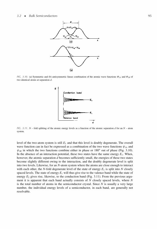
3.2 � Bulk Semiconductors 95
FIG. 3.10. (a) Symmetric and (b) antisymmetric linear combination of the atomic wave functions �1A and �1B oftwo identical atoms at separation d.
FIG. 3.11. N – fold splitting of the atomic energy levels as a function of the atomic separation d for an N – atomsystem.
level of the two-atom system is still E1 and that this level is doubly degenerate. The overallwave function can in fact be expressed as a combination of the two wave functions 1A and 1B in which the two functions combine either in phase or 180ı out of phase (Fig. 3.10).In the absence of an interaction potential, these two states have the same energy E1. When,however, the atomic separation d becomes sufficiently small, the energies of these two statesbecome slightly different owing to the interaction, and the doubly degenerate level is splitinto two levels. Likewise, for an N-atom system where the atoms are close enough to interactwith each other, the N-fold degenerate level of the state of energy E1 is split into N closelyspaced levels. The state of energy E1 will thus give rise to the valence band while the state ofenergy E2 gives rise, likewise, to the conduction band (Fig. 3.11). From the previous argu-ment it is apparent that each band actually consists of N closely spaced levels, where Nis the total number of atoms in the semiconductor crystal. Since N is usually a very largenumber, the individual energy levels of a semiconductor, in each band, are generally notresolvable.
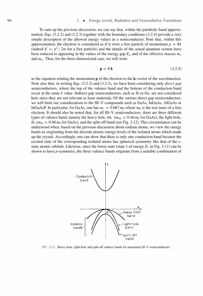
96 3 � Energy Levels, Radiative and Nonradiative Transitions
To sum up the previous discussion, we can say that, within the parabolic band approxi-mation, Eqs. (3.2.2) and (3.2.3) together with the boundary conditions (3.2.4) provide a verysimple description of the allowed energy values in a semiconductor. Note that, within thisapproximation, the electron is considered as if it were a free particle of momentum p D „k(indeed E D p2 = 2m for a free particle) and the details of the actual quantum system havebeen reduced to appearing in the values of the energy gap Eg and of the effective masses mc
and m� . Thus, for the three-dimensional case, we will write
p D „ k (3.2.5)
as the equation relating the momentum p of the electron to the k-vector of the wavefunction.Note also that, in writing Eqs. (3.2.2) and (3.2.3), we have been considering only direct gapsemiconductors, where the top of the valence band and the bottom of the conduction bandoccur at the same k value. Indirect gap semiconductors, such as Si or Ge, are not consideredhere since they are not relevant as laser materials. Of the various direct gap semiconductors,we will limit our considerations to the III–V compounds such as GaAs, InGaAs, AlGaAs orInGaAsP. In particular, for GaAs, one has mc D 0.067 m0 where m0 is the rest mass of a freeelectron. It should also be noted that, for all III–V semiconductors, there are three differenttypes of valence band, namely the heavy hole, hh, .mhh D 0.46 m0 for GaAs), the light hole,lh, (mlh D 0.08 m0 for GaAs), and the split-off band (see Fig. 3.12). This circumstance can beunderstood when, based on the previous discussion about sodium atoms, we view the energybands as originating from the discrete atomic energy levels of the isolated atoms which madeup the crystal. Accordingly, one can show that there is only one conduction band because theexcited state of the corresponding isolated atoms has spherical symmetry like that of the s-state atomic orbitals. Likewise, since the lower state (state 1 of energy E1 in Fig. 3.11) can beshown to have p-symmetry, the three valence bands originate from a suitable combination of
FIG. 3.12. Heavy-hole, light-hole and split-off valence bands for unstrained III–V semiconductors.
3.2 � Bulk Semiconductors 97
the px, py and pz orbitals of this state, account being taken of the crystal’s symmetry. Actuallyin a crystal of cubic symmetry such as in all unstrained III–V compounds, the three bandsare expected to have the same energy at k D 0. However, spin-orbit interactions lower oneof these bands, the split-off band, by an amount corresponding to �E D 0.34 eV for GaAs.Since this value is much larger than kTŒŠ0.028 eV�, the split-off band will always be filledwith electrons and will not participate in radiative and non-radiative transitions. For reasonswhich will be explained in the next section, the light hole band also makes little contributionto these transitions. Thus, to first order, the valence band of a III–V semiconductor can bethought to be made of only the heavy hole band.
3.2.2. Density of States
Following what was done for the cavity modes in Sect. 2.2.1, we can now proceed tocalculating the number of energy states, p.k/, whose k value ranges from 0 to k. With ref-erence to Fig. 2.2, since now both positive and negative values of ki are allowed, p.k/ isgiven by the volume of the sphere of radius k, 4 k3 = 3, divided by the volume of the unitcell, .2 /3 = LxLyLz, times a factor 2 to account for the two states arising from the electronspin. Thus
p .k/ D .k3V = 3 2/ (3.2.6)
where V D Lx Ly Lz is the crystal volume. Since the number of states is very large, we cancalculate the density of states per unit volume, � .k/, as
�c,v D d p
V d kD k2
2(3.2.7)
where Eq. (3.2.6) has been used. Note that this expression is valid for both the valence andconduction bands and, to indicate this, the density of states has been denoted with both indicesc and v. We are also interested in calculating the density of states, � .E/, in terms of theelectron energy. Since �c,v .E/ dE D �c,v .k/ dk, from Eq. (3.2.2) we obtain
�c .Ec/ D 1
2 2
�2 mc
„2
�3=2
E1=2c (3.2.8a)
�v .Ev/ D 1
2 2
�2 mv
„2
�3=2
E1=2v (3.2.8b)
We recall that Ec and Ev are measured from the bottom of the conduction and the top ofthe valence bands, upwards and downwards, respectively (Fig. 3.9a). One notes that, sincefor III–V compounds, one has mc << mv D mhh, then it follows that �c << �v. Onealso notes that, since mlh << mhh, the density of states of light holes is only a small frac-tion of that of heavy holes. Accordingly, the light holes are very much in a minority for aIII–V semiconductor, and their presence can normally be neglected in comparison with heavyholes.
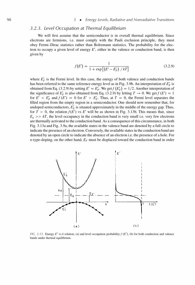
98 3 � Energy Levels, Radiative and Nonradiative Transitions
3.2.3. Level Occupation at Thermal Equilibrium
We will first assume that the semiconductor is in overall thermal equilibrium. Sinceelectrons are fermions, i.e. must comply with the Pauli exclusion principle, they mustobey Fermi–Dirac statistics rather than Boltzmann statistics. The probability for the elec-tron to occupy a given level of energy E0, either in the valence or conduction band, is thengiven by
fE0� D 1
1 C exp�
E0 � E0F
�= kT
(3.2.9)
where E0F is the Fermi level. In this case, the energy of both valence and conduction bands
has been referred to the same reference energy level as in Fig. 3.9b. An interpretation of E0F is
obtained from Eq. (3.2.9) by setting E0 D E0F. We get f
E0
F
� D 1=2. Another interpretation ofthe significance of E0
F is also obtained from Eq. (3.2.9) by letting T ! 0. We get f .E0/ D 1for E0 < E0
F and f .E0/ D 0 for E0 > E0F. Thus, at T D 0, the Fermi level separates the
filled region from the empty region in a semiconductor. One should now remember that, forundoped semiconductors, E0
F is situated approximately in the middle of the energy gap. Thus,for T > 0, the relation f .E0/ vs E0 will be as shown in Fig. 3.13b. This means that, sinceEg >> kT , the level occupancy in the conduction band is very small i.e. very few electronsare thermally activated to the conduction band. As a consequence of this circumstance, in bothFig. 3.13a and Fig. 3.9a, the available states in the valence band are denoted by a full circle toindicate the presence of an electron. Conversely, the available states in the conduction band aredenoted by an open circle to indicate the absence of an electron i.e. the presence of a hole. Forn-type-doping, on the other hand, EF must be displaced toward the conduction band in order
FIG. 3.13. Energy E0 vs k relation, (a) and level occupation probability f .E0/, (b) for both conduction and valencebands under thermal equilibrium.
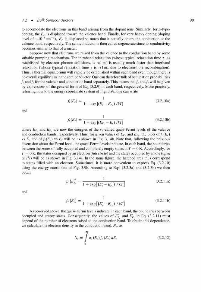
3.2 � Bulk Semiconductors 99
to accomodate the electrons in this band arising from the dopant ions. Similarly, for p-type-doping, the EF is displaced toward the valence band. Finally, for very heavy doping (dopinglevel of �1018 cm�3/, EF is displaced so much that it actually enters the conduction or thevalence band, respectively. The semiconductor is then called degenerate since its conductivitybecomes similar to that of a metal.
Suppose now that electrons are raised from the valence to the conduction band by somesuitable pumping mechanism. The intraband relaxation (whose typical relaxation time � , asestablished by electron–phonon collisions, is �1 ps) is usually much faster than interbandrelaxation (whose typical relaxation time � is �1 ns, due to electron-hole recombination).Thus, a thermal equilibrium will rapidly be established within each band even though there isno overall equilibrium in the semiconductor. One can therefore talk of occupation probabilitiesfv and fc for the valence and conduction band separately. This means that fc and fv will be givenby expressions of the general form of Eq. (3.2.9) in each band, respectively. More precisely,referring now to the energy coordinate system of Fig. 3.9a, one can write
fc.Ec/ D 1
1 C exp Œ.Ec � EFc/ =kT�(3.2.10a)
and
fv.Ev/ D 1
1 C exp Œ.EFv � Ev/ =kT�(3.2.10b)
where EFc and EFv are now the energies of the so-called quasi-Fermi levels of the valenceand conduction bands, respectively. Thus, for given values of EFc and EFv , the plots of fc.Ec/
vs Ec and of fv.Ev/ vs Ev will be as shown in Fig. 3.14b. Note that, following the previousdiscussion about the Fermi level, the quasi-Fermi levels indicate, in each band, the boundariesbetween the zones of fully occupied and completely empty states at T D 0 K. Accordingly, forT D 0 K, the states occupied by an electron (full circle) and the states occupied by a hole (opencircle) will be as shown in Fig. 3.14a. In the same figure, the hatched area thus correspondto states filled with an electron. Sometimes, it is more convenient to express Eq. (3.2.10)using the energy coordinate of Fig. 3.9b. According to Eqs. (3.2.3a) and (3.2.3b) we thenobtain
fcE0
c
� D 1
1 C exp�
E0c � E0
Fc
�= kT
(3.2.11a)
and
fvE0
v
� D 1
1 C exp�
E0v � E0
Fv
�= kT
(3.2.11b)
As observed above, the quasi-Fermi levels indicate, in each band, the boundaries betweenoccupied and empty states. Consequently, the values of E0
Fcand E0
Fvin Eq. (3.2.11) must
depend of the number of electrons raised to the conduction band. To obtain this dependence,we calculate the electron density in the conduction band, Ne, as
Ne D1Z
0
�c .Ec/ fc .Ec/ dEc (3.2.12)
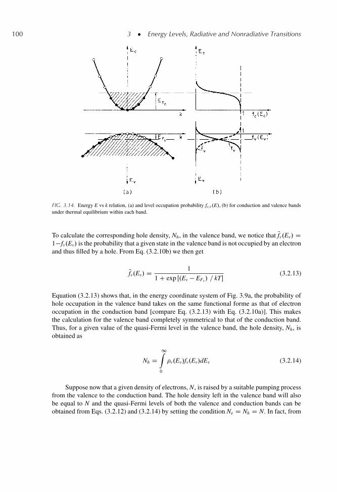
100 3 � Energy Levels, Radiative and Nonradiative Transitions
FIG. 3.14. Energy E vs k relation, (a) and level occupation probability fc,v.E/, (b) for conduction and valence bandsunder thermal equilibrium within each band.
To calculate the corresponding hole density, Nh, in the valence band, we notice that Nfv.Ev/ D1�fv.Ev/ is the probability that a given state in the valence band is not occupied by an electronand thus filled by a hole. From Eq. (3.2.10b) we then get
Nfv.Ev/ D 1
1 C exp Œ.Ev � EFv/ = kT�(3.2.13)
Equation (3.2.13) shows that, in the energy coordinate system of Fig. 3.9a, the probability ofhole occupation in the valence band takes on the same functional forme as that of electronoccupation in the conduction band [compare Eq. (3.2.13) with Eq. (3.2.10a)]. This makesthe calculation for the valence band completely symmetrical to that of the conduction band.Thus, for a given value of the quasi-Fermi level in the valence band, the hole density, Nh, isobtained as
Nh D1Z
0
�v.Ev/fv.Ev/dEv (3.2.14)
Suppose now that a given density of electrons, N, is raised by a suitable pumping processfrom the valence to the conduction band. The hole density left in the valence band will alsobe equal to N and the quasi-Fermi levels of both the valence and conduction bands can beobtained from Eqs. (3.2.12) and (3.2.14) by setting the condition Ne D Nh D N. In fact, from
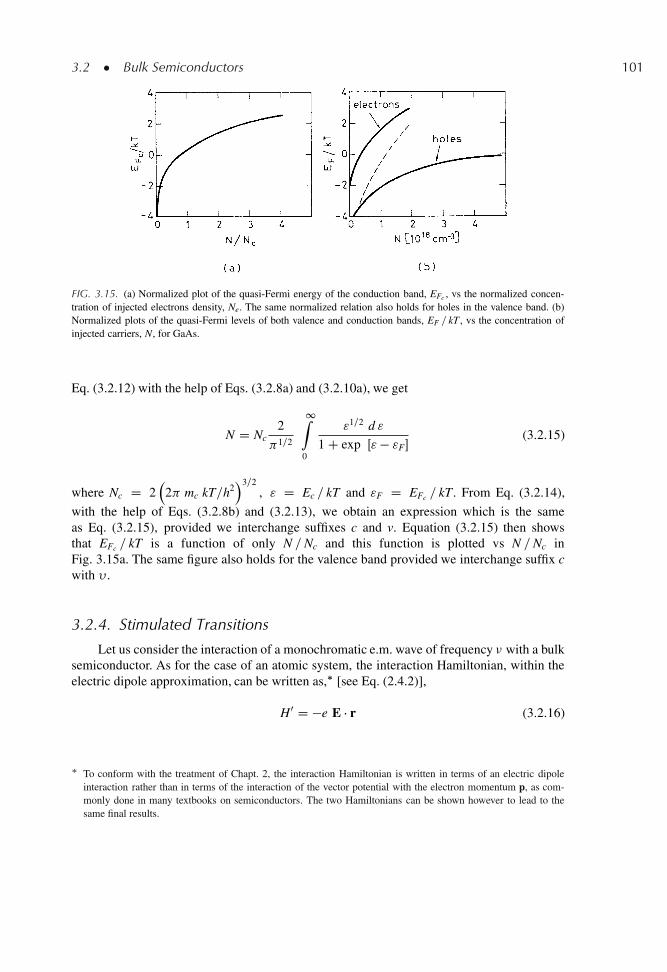
3.2 � Bulk Semiconductors 101
FIG. 3.15. (a) Normalized plot of the quasi-Fermi energy of the conduction band, EFc , vs the normalized concen-tration of injected electrons density, Ne. The same normalized relation also holds for holes in the valence band. (b)Normalized plots of the quasi-Fermi levels of both valence and conduction bands, EF = kT , vs the concentration ofinjected carriers, N, for GaAs.
Eq. (3.2.12) with the help of Eqs. (3.2.8a) and (3.2.10a), we get
N D Nc2
1=2
1Z0
"1=2 d "
1 C exp Œ" � "F�(3.2.15)
where Nc D 2�
2 mc kT=h2�3=2
, " D Ec = kT and "F D EFc = kT. From Eq. (3.2.14),
with the help of Eqs. (3.2.8b) and (3.2.13), we obtain an expression which is the sameas Eq. (3.2.15), provided we interchange suffixes c and v. Equation (3.2.15) then showsthat EFc = kT is a function of only N =Nc and this function is plotted vs N =Nc inFig. 3.15a. The same figure also holds for the valence band provided we interchange suffix cwith � .
3.2.4. Stimulated Transitions
Let us consider the interaction of a monochromatic e.m. wave of frequency � with a bulksemiconductor. As for the case of an atomic system, the interaction Hamiltonian, within theelectric dipole approximation, can be written as,� [see Eq. (2.4.2)],
H0 D �e E � r (3.2.16)
� To conform with the treatment of Chapt. 2, the interaction Hamiltonian is written in terms of an electric dipoleinteraction rather than in terms of the interaction of the vector potential with the electron momentum p, as com-monly done in many textbooks on semiconductors. The two Hamiltonians can be shown however to lead to thesame final results.
102 3 � Energy Levels, Radiative and Nonradiative Transitions
Example 3.4. Calculation of the quasi-Fermi energies forGaAs. We take mc D 0.067m0 and mv D mhh D 0.46m0
and assume T D 300 K. We get Nc D 4.12 � 1017 cm�3
and Nv D .mv =mc/3=2Nc D 7.41 � 1018 cm�3, where Nc
is the electron concentration defined in connection withEq. (3.2.15) and Nv is the corresponding quantity for theholes. At each electron concentration, N, one can nowobtain the quantity N =Nc and, from the general plot ofFig. 3.15a, deduce the corresponding quantity EFc = kT. Asimilar calculation can be made for the holes. The valuesof EF = kT, calculated in this way for both electrons andholes in GaAs, are plotted in Fig. 3.15b vs the carrierconcentration, N.
where E D E.r, t/ is the electric field of thee.m. wave at position r and time t. For a planewave, its expression can be written as
E D E0 exp j.kopt � r � ! t/ (3.2.17)
where kopt is the field wave vector and ! D2 �. If � Eg = h a transition may occurfrom a state in the valence band to a state inthe conduction band. If we let E0
2 and E01 be
the corresponding energies of the two states,the transition rate W, according to Eq. (A. 23)of Appendix A, is
W D 2
„2
ˇH0o
12
ˇ2ı .� � �o/ (3.2.18)
where �0 D .E02 � E0
1/ = h and
ˇH0o
12
ˇ2 Dˇˇ Z �
c
�er � E0 ej kopt�r� vdV
ˇˇ2 (3.2.19)
Note that v and c in Eq. (3.2.19) are the Bloch wave functions of levels 1 and 2 as given byEq. (3.2.1).
From Eqs. (3.2.18) and (3.2.19) we can now obtain the selection rules for the interaction.From Eq. (3.2.18), noting the ı-Dirac function on the right hand side, one sees that � D �0.This means that
E0
2 � E0� D h � (3.2.20)
which is often referred to as the energy conservation rule for the interaction. Similarly, fromEq. (3.2.19), since v / exp.jkv � r/ and c / exp.ikc � r/ one can show that the integral isnon-vanishing only when
kc D kopt C kv (3.2.21)
The proof of Eq. (3.2.21) is somewhat involved and requires that the periodic properties ofuc.r/ and uv.r/ appearing in Eq. (3.2.1) be properly taken into account..15/ The selection ruleEq. (3.3.21) can however be physically understood when we notice that an exponential factorof the form exp j
�kv C kopt � kc
� � r
is present in the integrand of Eq. (3.3.19) and thisterm, since it oscillates rapidly with r, makes the value of the integral zero unless kv C kopt �kc D 0. Since „kc,v is the electron momentum in the conduction or valence band and „kopt
is the photon momentum, Eq. (3.2.21) shows that the total momentum must be conserved inthe transition. One should note that one has kopt D 2 n = � where n is the semiconductorrefractive index and � is the transition wavelength. Thus, with e.g. n D 3.5 and � Š 1�m,one has kopt Š 105 cm�1. On the other hand one typically has kc,v D 106 � 107 cm�1 for
3.2 � Bulk Semiconductors 103
an electron or hole of average thermal energy (see Example 3.5). Thus kopt << kc,v andEq. (3.2.21) simplifies to
kc D kv (3.2.22)
Equation (3.2.22) is often referred to as the k-selection or k-conservation rule and indicatesthat stimulated transitions must occur vertically in the E vs k diagram (see Fig. 3.13a). Notefinally that the e.m. wave does not interact with the electron’s spin or, in other words, that spinis not involved in the interaction Hamiltonian Eq. (3.2.16). The spin, therefore, cannot changein the transition i.e. the selection rule for the change of the electron spin, � S, is simply
� S D 0 (3.2.23)
Example 3.5. Calculation of typical values of k for athermal electron. For an electron in the conduction bandhaving average thermal velocity �th, one has mc�
2th D
3 k T where T is the electron temperature. We also havep D „ kc D mc�th. Combining the two previous expres-sions, we get kc D Œ3mckT�1=2 =„. If we take mc D0.067 m0, as for GaAs, and kT D 0.028 eV .T Š 300 K/we thus get kc D 2.7 � 106 cm�1. Similarly one haskv D Œ3mvkT�1=2 =„ and thus kv D .mv = mc/
1=2 kc Š7 � 106 cm�1 if we take mc D mhh D 0.46 m0 for GaAs.
As for the case of atomic transitions consid-ered in the previous Chapter, Eq. (3.2.18)needs to be modified when line broaden-ing mechanisms are taken into account. Forsemiconductors, the main broadening mech-anism arises from electron-phonon dephas-ing collisions. Thus the ı-Dirac function inEq. (3.2.18) must be replaced by a Lorentzianfunction g.���0/, whose width, according toEq. (2.5.11) is given by ��0 D 1= �c where�c is the average electron-phonon dephasingcollision time (�c Š 0.1 ps for GaAs). Pro-ceeding as in Sect. 2.4.4, we can arrive at a definition of a transition cross section which hasthe same form as for atomic transitions,� namely [see also Eq. (2.4.18)]
� D 2 2 �
n"0ch
�2
3g .� � �0/ (3.2.24)
where � D jμj and
μ DZ
uceruvdV (3.2.25)
where uc D uck amd uv D uvk are the Bloch wavefunctions, appearing in Eq. (3.2.1). Note thefactor 3 in the term �2 = 3 of Eq. (3.3.24) which arises from averaging the matrix element μ
over all electron k vector directions, for a fixed electric field polarization [in this regard, seefootnote appearing in connection with Eqs. (2.4.13).
� Note that the concept of cross section as discussed in connection with Fig. 2.7 loses its meaning for a delocalizedwavefunction such as the Bloch wavefunction. We nevertheless retain the same symbol � for a semiconductor tomake an easier comparison with the case of isolated atoms or ions. Here � has the only meaning that the transitionrate for a plane wave is W D �F, where F is the photon flux of the wave or, alternatively, W D �� c=h�, where �is the energy density and � is the frequency of the wave.
104 3 � Energy Levels, Radiative and Nonradiative Transitions
3.2.5. Absorption and Gain Coefficients
Consider first two energy levels, E02 and E0
1, in the conduction and valence band, respec-tively, whose energy difference is equal to E0 D h�0, where �0 is the frequency of thetransition. Under the k-selection rule given by Eq. (3.2.22), the energies E0
2 and E01 are
uniquely established for a given value of �0. In fact, from Eqs. (3.2.3) and (3.2.2), one writes
E02 D Eg C .„2k2 = 2mc/ (3.2.26a)
E01 D �„2k2 = 2mv (3.2.26b)
where we have set k D kc D kv. From Eq. (3.2.26), since E02 � E0
1 D E0 D h�0, we obtain
h�0 D Eg C .„2k2 = 2mr/ (3.2.26c)
where mr is the reduced mass of the semiconductor, given by the relation m�1r D m�1
c C m�1v .
Equation (3.2.26) constitute a set of three equations in the three unknowns E02, E0
1 and k.As a next step, we define the joint density of states with respect to the energy variable
E0 D E02�E0
1 so that �jdE0 gives the density of transitions with transition energy lying betweenE0 and E0 C dE0. Under the k-selection and spin selection rules given by Eqs. (3.2.22) and(3.2.23), any state in e.g. the valence band, with a given spin, is coupled to only one state in theconduction band with the same spin. The number of transitions is thus equal to the number ofcorresponding states in either valence or conduction bands. We thus write �jdE0 D � .k/ dk,where � .k/ D �c,v .k/ is given by Eq. (3.2.7), so that we obtain
� j .E0/ D k2 = 2
�.dk = d E0/ (3.2.27)
With the help of Eq. (3.2.26c), Eq. (3.2.27) gives
� j .E0/ D 1
2 2
�2mr
„2
�3=2 E0 � Eg
�1=2(3.2.28)
For our purposes it is better to introduce the joint density of states, �j .�0/, with respect to thetransition frequency �0 D E0 = h. Since �j .�0/ d �0 D �j .E0/ dE0, we get from Eq. (3.2.28)
� j.� 0/ D 4
h2.2mr/
3=2 �h�0 � Eg1=2
(3.2.29)
Consider now the elemental number of transitions dN D �j .�0/ d�0 whose transitionfrequency lies between �0 and �0 C d�0. For absorption to occur, the lower level, of energyE0
1, must be occupied by an electron while the upper level, of energy E02, must be empty. The
number of transitions available for absorption will thus be
dNa D .dN/ fvE0
1
��1 � fc
E0
2
�(3.2.30)
where fvE0
1
�is the probability that the lower level is full while
�1 � fc
E0
2
�is the probability
that the upper level is empty. Note that a general case of equilibrium within each band isassumed so that fv
E0
1
�and fc
E0
2
�are obtained by Eqs. (3.2.11b) and (3.2.11a) with E0
v and
3.2 � Bulk Semiconductors 105
E0c being substituted by E0
1 and E02 respectively. To calculate the net absorption, we must also
take into account the process of stimulated emission between the same two levels. This willoccur when the upper state is full while the lower state is empty. The number of transitionsavailable for stimulated emission will then be
dNse D .dN/ fcE0
2
��1 � fv
E0
1
�(3.2.31)
Once the elemental numbers of available transitions for absorption and stimulated emissionare calculated, the absorption coefficient at frequency � is obtained, via (2.4.32), as d˛ D� .� � �0/ .dNa � dNse/, where � D �h is the homogeneous cross section for the E0
1 ! E02
transition. From Eq. (3.2.24) we then get
d˛ D�
2 2�
n"0ch
��2
3g .� � �0/ �j .�0/
�fvE0
1
� � fcE0
2
�d�0 (3.2.32)
The overall absorption coefficient at frequency � is obtained from Eq. (3.2.32) by integratingover all transition frequencies �0. If we assume that g .� � �0/ vs �0 is a much narrowerfunction than both �j .�0/ and .fc � fv/, than g .� � �0/ can be approximated by a ı function,ı D ı .� � �0/. We then get
˛ D�
2 2�
n"0ch
��2
3�j .�/
�fvE0
1
� � fcE0
2
�(3.2.33)
where E02 and E0
1 are now the energies of the two levels whose energy difference is h�. Theycan be readily calculated from Eq. (3.2.36) by substituting h�0 with h�.
According to Eq. (3.2.33), the absorption coefficient ˛ D ˛.�/ can be written as
˛ D ˛0�fv.E
01/ � fc.E
02/
(3.2.34)
where
˛0 D�
2 2�
n"0ch
��2
3�j.�/ (3.2.35)
The meaning of ˛0 D ˛0.�/ is understood when we consider a semiconductor in overallthermal equilibrium at T D 0 K. The quasi-Fermi levels coincide in this case with the Fermi-level and, if this level is within the energy gap, one has fv
E0
1
� D 1 and fcE0
2
� D 1. One thenhas ˛.�/ D ˛0.�/ which is the maximum absorption coefficient that the semiconductor canhave at frequency �. Note that, for an intrinsic semiconductor and assuming Eg >> kT as isthe case for all III–V semiconductors, we still have fv
E0
1
� Š 1 and fcE0
2
� Š 0 i.e. ˛ Š ˛0
even at room temperature. From Eq. (3.2.35), with the help of Eq. (3.2.29) with �0 substitutedby �, we then get
˛ Š ˛0 D 3 �
n"0ch3
�2
3.2mr/
3=2 �h� � Eg1=2
(3.2.36)
The frequency behaviour of ˛.�/ is then determined, to a good approximation, simply by the
frequency behaviour ofh� � Eg
�1=2.
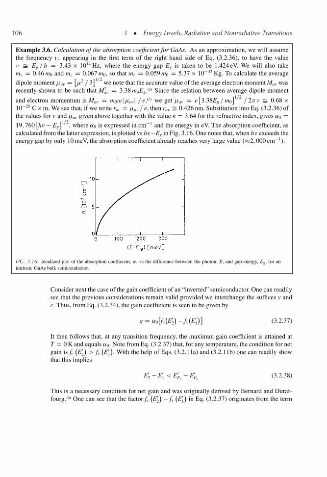
106 3 � Energy Levels, Radiative and Nonradiative Transitions
Example 3.6. Calculation of the absorption coefficient for GaAs. As an approximation, we will assumethe frequency �, appearing in the first term of the right hand side of Eq. (3.2.36), to have the value� Š Eg = h D 3.43 � 1014 Hz, where the energy gap Eg is taken to be 1.424 eV. We will also takemv D 0.46 m0 and mc D 0.067 m0, so that mr D 0.059 m0 D 5.37 � 10�32 Kg. To calculate the average
dipole moment�av D ��2 = 3
1=2we note that the accurate value of the average electron moment Mav was
recently shown to be such that M2av D 3.38 moEg..5/ Since the relation between average dipole moment
and electron momentum is Mav D m0! j�avj = e,.5/ we get �av D e�3.38Eg =m0
1=2= 2 � Š 0.68 �
10�25 C � m. We see that, if we write rav D �av = e, then rav Š 0.426 nm. Substitution into Eq. (3.2.36) ofthe values for � and �av given above together with the value n D 3.64 for the refractive index, gives ˛0 D19, 760
�h� � Eg
1=2, where ˛0 is expressed in cm�1 and the energy in eV. The absorption coefficient, as
calculated from the latter expression, is plotted vs h��Eg in Fig. 3.16. One notes that, when h� exceeds theenergy gap by only 10 meV, the absorption coefficient already reaches very large value .�2, 000 cm�1/.
FIG. 3.16. Idealized plot of the absorption coefficient, ˛, vs the difference between the photon, E, and gap energy, Eg, for anintrinsic GaAs bulk semiconductor.
Consider next the case of the gain coefficient of an “inverted” semiconductor. One can readilysee that the previous considerations remain valid provided we interchange the suffices v andc. Thus, from Eq. (3.2.34), the gain coefficient is seen to be given by
g D ˛0�fcE0
2
� � fvE0
1
�(3.2.37)
It then follows that, at any transition frequency, the maximun gain coefficient is attained atT D 0 K and equals ˛0. Note from Eq. (3.2.37) that, for any temperature, the condition for netgain is fc
E0
2
�> fv
E0
1
�. With the help of Eqs. (3.2.11a) and (3.2.11b) one can readily show
that this implies
E02 � E0
1 < E0Fc
� E0Fv
(3.2.38)
This is a necessary condition for net gain and was originally derived by Bernard and Duraf-fourg..6/ One can see that the factor fc
E0
2
� � fvE0
1
�in Eq. (3.2.37) originates from the term
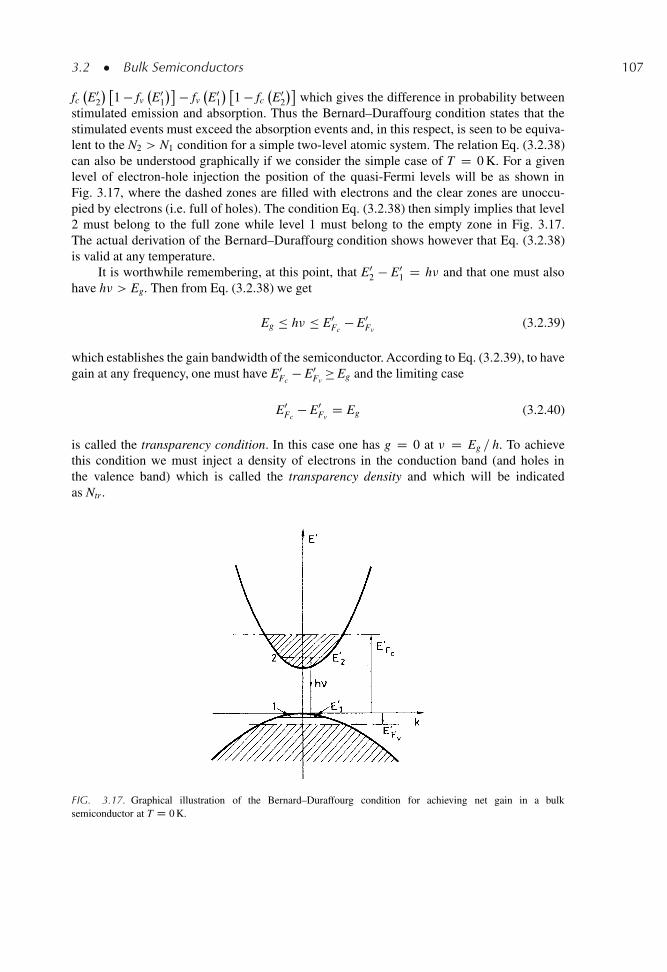
3.2 � Bulk Semiconductors 107
fcE0
2
� �1 � fv
E0
1
� � fvE0
1
� �1 � fc
E0
2
�which gives the difference in probability between
stimulated emission and absorption. Thus the Bernard–Duraffourg condition states that thestimulated events must exceed the absorption events and, in this respect, is seen to be equiva-lent to the N2 > N1 condition for a simple two-level atomic system. The relation Eq. (3.2.38)can also be understood graphically if we consider the simple case of T D 0 K. For a givenlevel of electron-hole injection the position of the quasi-Fermi levels will be as shown inFig. 3.17, where the dashed zones are filled with electrons and the clear zones are unoccu-pied by electrons (i.e. full of holes). The condition Eq. (3.2.38) then simply implies that level2 must belong to the full zone while level 1 must belong to the empty zone in Fig. 3.17.The actual derivation of the Bernard–Duraffourg condition shows however that Eq. (3.2.38)is valid at any temperature.
It is worthwhile remembering, at this point, that E02 � E0
1 D h� and that one must alsohave h� > Eg. Then from Eq. (3.2.38) we get
Eg h� E0Fc
� E0Fv
(3.2.39)
which establishes the gain bandwidth of the semiconductor. According to Eq. (3.2.39), to havegain at any frequency, one must have E0
Fc� E0
Fv Eg and the limiting case
E0Fc
� E0Fv
D Eg (3.2.40)
is called the transparency condition. In this case one has g D 0 at � D Eg = h. To achievethis condition we must inject a density of electrons in the conduction band (and holes inthe valence band) which is called the transparency density and which will be indicatedas Ntr .
FIG. 3.17. Graphical illustration of the Bernard–Duraffourg condition for achieving net gain in a bulksemiconductor at T D 0 K.
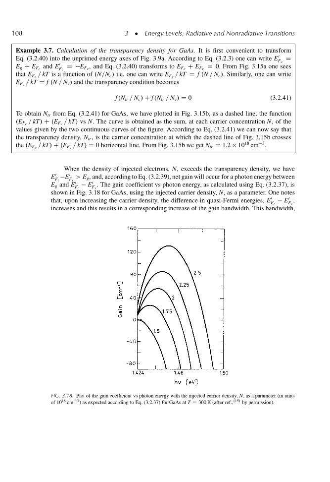
108 3 � Energy Levels, Radiative and Nonradiative Transitions
Example 3.7. Calculation of the transparency density for GaAs. It is first convenient to transformEq. (3.2.40) into the unprimed energy axes of Fig. 3.9a. According to Eq. (3.2.3) one can write E0
FcD
Eg C EFc and E0Fv
D �EFv , and Eq. (3.2.40) transforms to EFc C EFv D 0. From Fig. 3.15a one seesthat EFc = kT is a function of .N=Nc/ i.e. one can write EFc = kT D f .N =Nc/. Similarly, one can writeEFv = kT D f .N =Nv/ and the transparency condition becomes
f .Ntr =Nc/C f .Ntr =Nv/ D 0 (3.2.41)
To obtain Ntr from Eq. (3.2.41) for GaAs, we have plotted in Fig. 3.15b, as a dashed line, the function.EFc = kT/ C .EFv = kT/ vs N. The curve is obtained as the sum, at each carrier concentration N, of thevalues given by the two continuous curves of the figure. According to Eq. (3.2.41) we can now say thatthe transparency density, Ntr , is the carrier concentration at which the dashed line of Fig. 3.15b crossesthe .EFc = kT/C .EFv = kT/ D 0 horizontal line. From Fig. 3.15b we get Ntr D 1.2 � 1018 cm�3.
When the density of injected electrons, N, exceeds the transparency density, we haveE0
Fc�E0
Fv> Eg, and, according to Eq. (3.2.39), net gain will occur for a photon energy between
Eg and E0Fc
� E0Fv
. The gain coefficient vs photon energy, as calculated using Eq. (3.2.37), isshown in Fig. 3.18 for GaAs, using the injected carrier density, N, as a parameter. One notesthat, upon increasing the carrier density, the difference in quasi-Fermi energies, E0
Fc� E0
Fv,
increases and this results in a corresponding increase of the gain bandwidth. This bandwidth,
FIG. 3.18. Plot of the gain coefficient vs photon energy with the injected carrier density, N, as a parameter (in unitsof 1018 cm�3) as expected according to Eq. (3.2.37) for GaAs at T D 300 K (after ref.,.15/ by permission).
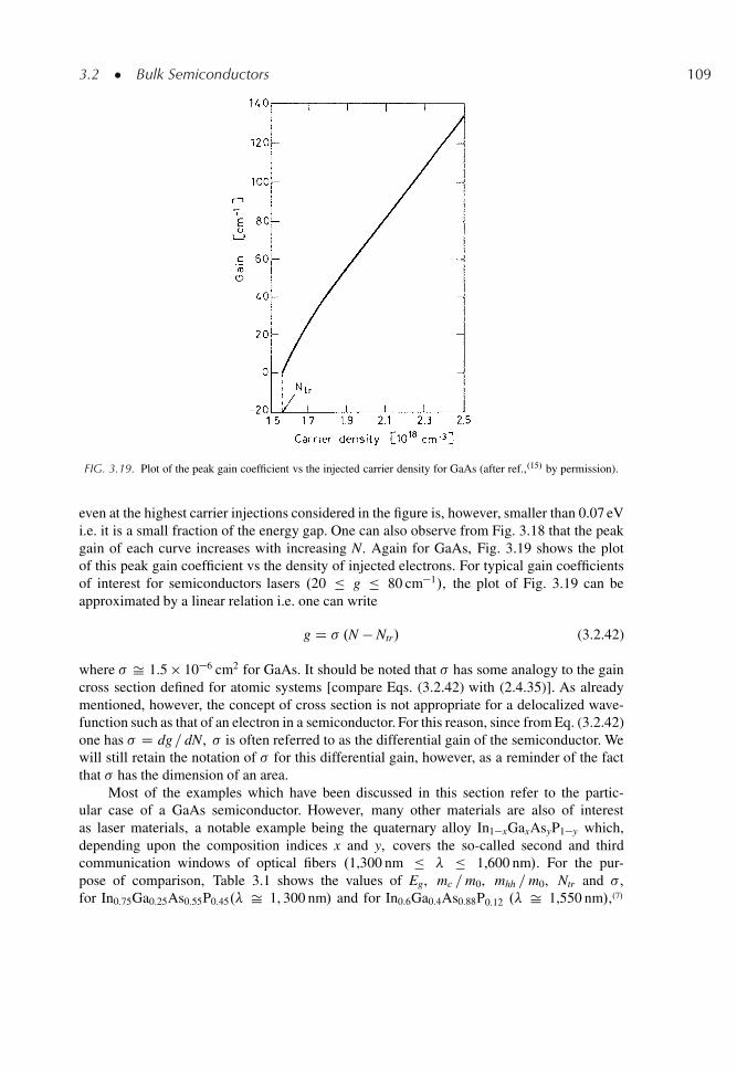
3.2 � Bulk Semiconductors 109
FIG. 3.19. Plot of the peak gain coefficient vs the injected carrier density for GaAs (after ref.,.15/ by permission).
even at the highest carrier injections considered in the figure is, however, smaller than 0.07 eVi.e. it is a small fraction of the energy gap. One can also observe from Fig. 3.18 that the peakgain of each curve increases with increasing N. Again for GaAs, Fig. 3.19 shows the plotof this peak gain coefficient vs the density of injected electrons. For typical gain coefficientsof interest for semiconductors lasers .20 g 80 cm�1/, the plot of Fig. 3.19 can beapproximated by a linear relation i.e. one can write
g D � .N � Ntr/ (3.2.42)
where � Š 1.5 � 10�6 cm2 for GaAs. It should be noted that � has some analogy to the gaincross section defined for atomic systems [compare Eqs. (3.2.42) with (2.4.35)]. As alreadymentioned, however, the concept of cross section is not appropriate for a delocalized wave-function such as that of an electron in a semiconductor. For this reason, since from Eq. (3.2.42)one has � D dg = dN, � is often referred to as the differential gain of the semiconductor. Wewill still retain the notation of � for this differential gain, however, as a reminder of the factthat � has the dimension of an area.
Most of the examples which have been discussed in this section refer to the partic-ular case of a GaAs semiconductor. However, many other materials are also of interestas laser materials, a notable example being the quaternary alloy In1�xGaxAsyP1�y which,depending upon the composition indices x and y, covers the so-called second and thirdcommunication windows of optical fibers .1,300 nm � 1,600 nm/. For the pur-pose of comparison, Table 3.1 shows the values of Eg, mc =m0, mhh =m0, Ntr and � ,for In0.75Ga0.25As0.55P0.45.� Š 1, 300 nm/ and for In0.6Ga0.4As0.88P0.12 .� Š 1,550 nm/,.7/
110 3 � Energy Levels, Radiative and Nonradiative Transitions
TABLE 3.1. Values of emission wavelength, �, energy gap, Eg, conduction band electron mass, mc,heavy-hole, mhh, carrier density at transparency, Ntr, material differential gain, � , and lifetime � , for
GaAs .� Š 850 nm/, and InGaAsP (� D 1,300 and � D 1,550 nm) bulk semiconductors
GaAs In0.73Ga0.27As0.6P0.4 In0.58Ga0.42As0.9P0.1
� [nm] 840 1,310 1,550Eg [eV] 1.424 0.96 0.81mc=m0 0.067 0.058 0.046mhh=m0 0.46 0.467 0.44Ntr Œ1018 cm�3� 1.2 1 1�Œ10�16 cm2� 1.5 1.2 � 2.5 1.2 � 2.5� [ns] 3 4.5 4.5
as well as the corresponding values for GaAs, as discussed in this section. It should benoted that the reported values for Ntr and � fall in a range of values reported for thesesemiconductors and are included in Table 3.1 just as indicative numbers. It does seem, how-ever, that both Ntr and � for InGaAsP are somewhat smaller than the corresponding valuesfor GaAs.
3.2.6. Spontaneous Emission and Nonradiative Decay
Let us first consider the spontaneous emission process and define the spectral rateR� so that R�d� represents the number of spontaneous emission events per unit time andvolume which result in light emitted with frequency between � and � C d�. To calcu-late R� consider first the transitions, �j .�0/ d�0, whose transition frequencies lie between�0 and �0 C d�0. They will give an elemental contribution, d R� , to R� given by dR� DA21g .� � �0/ � ˚fc E0
20
� �1 � fv
E0
10
���j .�0/ d�0 where A21 D A21 .�0/ is the rate of spon-
taneous emission between the two levels and g .� � �0/ is the lineshape function of thetransition. It should be noted that �j .�0/ has been multiplied by fc
E0
20
� �1 � fv
E0
10
�since,
as for stimulated emission, spontaneous emission can only occur between an occupied upperstate and an empty lower state. The total spectral rate R� is then obtained by integrating theabove expression over all transition frequencies �0. Thus
R� DZ
A21g .� � �0/˚fcE0
2
� �1 � fv
E0
1
���j.�0/d�0 (3.2.43)
In the limit where g .� � �0/ can be considered a much narrower function of �0 than all otherfunctions in the integrand, g .� � �0/ can be approximated by a ı function ı .� � �0/ andEq. (3.2.43) reduces to
R� D A21˚fcE0
2
� �1 � fv
E0
1
���j.�/ (3.2.44)
where A21 is the spontaneous emission rate for �0 D � and E02 and E0
1 are now the energy levelscorresponding to a transition frequency �. As an example, Fig. 3.20 shows the qualitativebehaviour of R� vs the photon energy h� for an electron injection rate exceeding the rate for
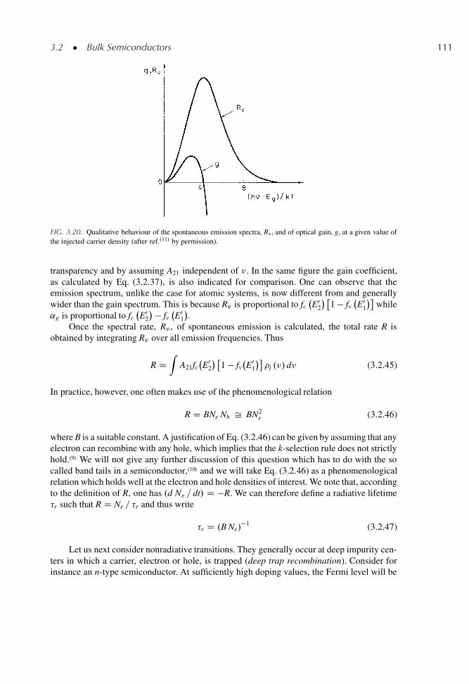
3.2 � Bulk Semiconductors 111
FIG. 3.20. Qualitative behaviour of the spontaneous emission spectra, Rv, and of optical gain, g, at a given value ofthe injected carrier density (after ref..11/ by permission).
transparency and by assuming A21 independent of �. In the same figure the gain coefficient,as calculated by Eq. (3.2.37), is also indicated for comparison. One can observe that theemission spectrum, unlike the case for atomic systems, is now different from and generallywider than the gain spectrum. This is because R� is proportional to fc
E0
2
� �1 � fv
E0
1
�while
˛g is proportional to fcE0
2
� � fvE0
1
�.
Once the spectral rate, R� , of spontaneous emission is calculated, the total rate R isobtained by integrating R� over all emission frequencies. Thus
R DZ
A21fcE0
2
� �1 � fv
E0
1
��j .�/ d� (3.2.45)
In practice, however, one often makes use of the phenomenological relation
R D BNe Nh Š BN2e (3.2.46)
where B is a suitable constant. A justification of Eq. (3.2.46) can be given by assuming that anyelectron can recombine with any hole, which implies that the k-selection rule does not strictlyhold..9/ We will not give any further discussion of this question which has to do with the socalled band tails in a semiconductor,.10/ and we will take Eq. (3.2.46) as a phenomenologicalrelation which holds well at the electron and hole densities of interest. We note that, accordingto the definition of R, one has .d Ne = dt/ D �R. We can therefore define a radiative lifetime�r such that R D Ne = �r and thus write
�r D .B Ne/�1 (3.2.47)
Let us next consider nonradiative transitions. They generally occur at deep impurity cen-ters in which a carrier, electron or hole, is trapped (deep trap recombination). Consider forinstance an n-type semiconductor. At sufficiently high doping values, the Fermi level will be
112 3 � Energy Levels, Radiative and Nonradiative Transitions
close enough to the conduction band that these traps will be filled with electrons. A nonra-diative transition then occurs by recombination of a free hole with this trapped electron, theexcess energy being given to the lattice. A similar argument applies for p-type-doping. Forsmall gap semiconductors, nonradiative transitions can also occur by direct recombinationof untrapped electrons and holes, the excess energy being given to another electron (or hole)which gets excited to a higher energy state in the band (Auger recombination.12/). Since Augerrecombination is a three-body process, the decay of electron density due to this procees canbe written phenomenologically as .dNe = dt/ D �CNeNhNe D �CN3
e , where C is a suitableconstant. Accordingly, we can define a nonradiative lifetime due to Auger recombination,�A, as
�A D �C N2
e
�1(3.2.48)
The dominant nonradiative mechanism seems to be deep-trap recombination for GaAs andAuger recombination in long wavelength semiconductor laser materials such as InGaAsP.
Example 3.8. Radiative and nonradiative lifetimes in GaAs and InGaAsP. For GaAs, we will take B Š1.8 � 10�10 cm3 s
�1and Ne Š Ntr D 1.2 � 1018 cm�3. We then get �r D 1 =B Ntr Š 4.6 ns, to be
compared with the measured overall lifetime, at transparency, of � Š 3 ns .T D 300 K/. Since ��1 D��1
r C ��1nr , where �nr is the lifetime due to the nonradiative process, we can infer a nonradiative lifetime
�nr, in this case due to deep-trap recombination, of about 9 ns. For InGaAsP at � D 1, 300 nm we takeB D 2 � 10�10 cm3 s
�1, Ne Š Ntr Š 1 � 1018 cm3 and C Š 3 � 10�29 cm6 s
�1. We get from Eq. (3.2.47)
�r Š 5 ns and from Eq. (3.2.48) �A Š 33.3 ns which gives an overall lifetime, � , in agreement with themeasured value [� Š 5 ns at T D 300 K].
3.2.7. Concluding Remarks
We have seen in this section that the phenomena leading to radiative and nonradiativetransitions in a bulk semiconductor are notably more complicated than those occurring forisolated atoms or ions, which were considered in the previous Chapter. From a practical view-point, however, the most important physical parameters which are needed to predict laserbehaviour are the differential gain � , the transparency density Ntr , and the overall lifetime �for spontaneous decay (resulting from both radiative and non radiative processes). For GaAsand for the InGaAs alloys considered here, these quantities can be obtained from Table 3.1.It should be reminded that the lifetime depends on the carrier concentration and the valuesreported in the table refer to a concentration equal to the transparency density.
In concluding this section we also recall that the gain value given by Eq. (3.2.37) refersto a semiconductor of large dimensions (bulk semiconductor). For this reason, the gain valuesquoted in Table 3.1 are often referred to as the material gain. The actual gain in a double-heterostructure laser is smaller than this and it is determined by the ratio of the transversedimension of the active layer to that of the cavity mode. This gain, often called the modalgain, thus depends on details of the laser configuration and will be considered in the relevantsection of Chap. 9 dealing with semiconductor lasers.
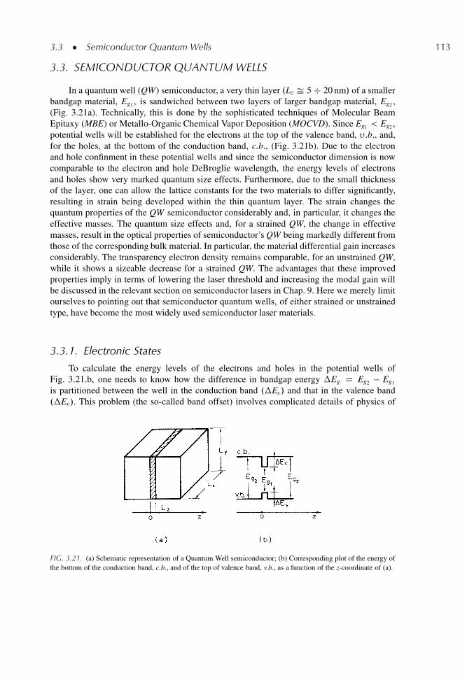
3.3 � Semiconductor Quantum Wells 113
3.3. SEMICONDUCTOR QUANTUM WELLS
In a quantum well (QW) semiconductor, a very thin layer .Lz Š 5 � 20 nm/ of a smallerbandgap material, Eg1 , is sandwiched between two layers of larger bandgap material, Eg2 ,(Fig. 3.21a). Technically, this is done by the sophisticated techniques of Molecular BeamEpitaxy (MBE) or Metallo-Organic Chemical Vapor Deposition (MOCVD). Since Eg1 < Eg2 ,potential wells will be established for the electrons at the top of the valence band, � .b., and,for the holes, at the bottom of the conduction band, c.b., (Fig. 3.21b). Due to the electronand hole confinment in these potential wells and since the semiconductor dimension is nowcomparable to the electron and hole DeBroglie wavelength, the energy levels of electronsand holes show very marked quantum size effects. Furthermore, due to the small thicknessof the layer, one can allow the lattice constants for the two materials to differ significantly,resulting in strain being developed within the thin quantum layer. The strain changes thequantum properties of the QW semiconductor considerably and, in particular, it changes theeffective masses. The quantum size effects and, for a strained QW, the change in effectivemasses, result in the optical properties of semiconductor’s QW being markedly different fromthose of the corresponding bulk material. In particular, the material differential gain increasesconsiderably. The transparency electron density remains comparable, for an unstrained QW,while it shows a sizeable decrease for a strained QW. The advantages that these improvedproperties imply in terms of lowering the laser threshold and increasing the modal gain willbe discussed in the relevant section on semiconductor lasers in Chap. 9. Here we merely limitourselves to pointing out that semiconductor quantum wells, of either strained or unstrainedtype, have become the most widely used semiconductor laser materials.
3.3.1. Electronic States
To calculate the energy levels of the electrons and holes in the potential wells ofFig. 3.21.b, one needs to know how the difference in bandgap energy �Eg D Eg2 � Eg1
is partitioned between the well in the conduction band .�Ec/ and that in the valence band.�Ev/. This problem (the so-called band offset) involves complicated details of physics of
FIG. 3.21. (a) Schematic representation of a Quantum Well semiconductor; (b) Corresponding plot of the energy ofthe bottom of the conduction band, c.b., and of the top of valence band, v.b., as a function of the z-coordinate of (a).
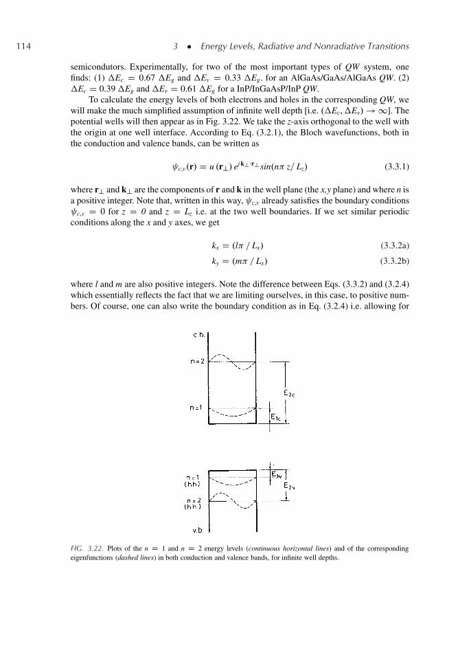
114 3 � Energy Levels, Radiative and Nonradiative Transitions
semicondutors. Experimentally, for two of the most important types of QW system, onefinds: (1) �Ec D 0.67 �Eg and �Ev D 0.33 �Eg. for an AlGaAs/GaAs/AlGaAs QW. (2)�Ec D 0.39�Eg and�Ev D 0.61�Eg for a InP/InGaAsP/InP QW.
To calculate the energy levels of both electrons and holes in the corresponding QW, wewill make the much simplified assumption of infinite well depth [i.e. .�Ec,�Ev/ ! 1]. Thepotential wells will then appear as in Fig. 3.22. We take the z-axis orthogonal to the well withthe origin at one well interface. According to Eq. (3.2.1), the Bloch wavefunctions, both inthe conduction and valence bands, can be written as
c,v.r/ D u .r?/ ej k?�r? sin.n z= Lz/ (3.3.1)
where r? and k? are the components of r and k in the well plane (the x,y plane) and where n isa positive integer. Note that, written in this way, c,v already satisfies the boundary conditions c,v D 0 for z D 0 and z D Lz i.e. at the two well boundaries. If we set similar periodicconditions along the x and y axes, we get
kx D .l = Lx/ (3.3.2a)
ky D .m = Lx/ (3.3.2b)
where l and m are also positive integers. Note the difference between Eqs. (3.3.2) and (3.2.4)which essentially reflects the fact that we are limiting ourselves, in this case, to positive num-bers. Of course, one can also write the boundary condition as in Eq. (3.2.4) i.e. allowing for
FIG. 3.22. Plots of the n D 1 and n D 2 energy levels (continuous horizontal lines) and of the correspondingeigenfunctions (dashed lines) in both conduction and valence bands, for infinite well depths.
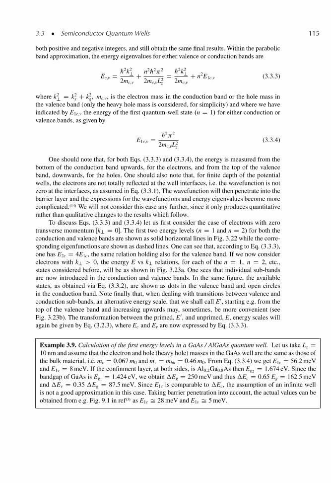
3.3 � Semiconductor Quantum Wells 115
both positive and negative integers, and still obtain the same final results. Within the parabolicband approximation, the energy eigenvalues for either valence or conduction bands are
Ec,v D „2k2?
2mc,vC n2„2 2
2mc,vL2z
D „2k2?
2mc,vC n2E1c,v (3.3.3)
where k2? D k2
x C k2g, mc,v, is the electron mass in the conduction band or the hole mass in
the valence band (only the heavy hole mass is considered, for simplicity) and where we haveindicated by E1c,v the energy of the first quantum-well state .n D 1/ for either conduction orvalence bands, as given by
E1c,v D „2 2
2mc,vL2z
(3.3.4)
One should note that, for both Eqs. (3.3.3) and (3.3.4), the energy is measured from thebottom of the conduction band upwards, for the electrons, and from the top of the valenceband, downwards, for the holes. One should also note that, for finite depth of the potentialwells, the electrons are not totally reflected at the well interfaces, i.e. the wavefunction is notzero at the interfaces, as assumed in Eq. (3.3.1). The wavefunction will then penetrate into thebarrier layer and the expressions for the wavefunctions and energy eigenvalues become morecomplicated..14/ We will not consider this case any further, since it only produces quantitativerather than qualitative changes to the results which follow.
To discuss Eqs. (3.3.3) and (3.3.4) let us first consider the case of electrons with zerotransverse momentum Œk? D 0�. The first two energy levels (n D 1 and n D 2) for both theconduction and valence bands are shown as solid horizontal lines in Fig. 3.22 while the corre-sponding eigenfunctions are shown as dashed lines. One can see that, according to Eq. (3.3.3),one has E2c D 4E1c, the same relation holding also for the valence band. If we now considerelectrons with k? > 0, the energy E vs k? relations, for each of the n D 1, n D 2, etc.,states considered before, will be as shown in Fig. 3.23a. One sees that individual sub-bandsare now introduced in the conduction and valence bands. In the same figure, the availablestates, as obtained via Eq. (3.3.2), are shown as dots in the valence band and open circlesin the conduction band. Note finally that, when dealing with transitions between valence andconduction sub-bands, an alternative energy scale, that we shall call E0, starting e.g. from thetop of the valence band and increasing upwards may, sometimes, be more convenient (seeFig. 3.23b). The transformation between the primed, E0, and unprimed, E, energy scales willagain be given by Eq. (3.2.3), where Ec and Ev are now expressed by Eq. (3.3.3).
Example 3.9. Calculation of the first energy levels in a GaAs / AlGaAs quantum well. Let us take Lz D10 nm and assume that the electron and hole (heavy hole) masses in the GaAs well are the same as those ofthe bulk material, i.e. mc D 0.067 m0 and mv D mhh D 0.46 m0. From Eq. (3.3.4) we get E1c D 56.2 meVand E1v D 8 meV. If the confinment layer, at both sides, is Al0.2Ga0.8As then Eg2 D 1.674 eV. Since thebandgap of GaAs is Eg1 D 1.424 eV, we obtain �Eg D 250 meV and thus �Ec D 0.65 Eg D 162.5 meVand �Ev D 0.35 �Eg D 87.5 meV. Since E1c is comparable to �Ec, the assumption of an infinite wellis not a good approximation in this case. Taking barrier penetration into account, the actual values can beobtained from e.g. Fig. 9.1 in ref.3/ as E1c Š 28 meV and E1v Š 5 meV.
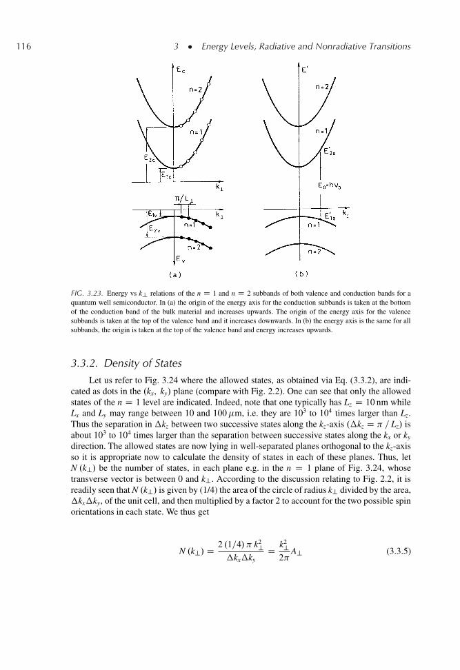
116 3 � Energy Levels, Radiative and Nonradiative Transitions
FIG. 3.23. Energy vs k? relations of the n D 1 and n D 2 subbands of both valence and conduction bands for aquantum well semiconductor. In (a) the origin of the energy axis for the conduction subbands is taken at the bottomof the conduction band of the bulk material and increases upwards. The origin of the energy axis for the valencesubbands is taken at the top of the valence band and it increases downwards. In (b) the energy axis is the same for allsubbands, the origin is taken at the top of the valence band and energy increases upwards.
3.3.2. Density of States
Let us refer to Fig. 3.24 where the allowed states, as obtained via Eq. (3.3.2), are indi-cated as dots in the .kx, ky/ plane (compare with Fig. 2.2). One can see that only the allowedstates of the n D 1 level are indicated. Indeed, note that one typically has Lz D 10 nm whileLx and Ly may range between 10 and 100�m, i.e. they are 103 to 104 times larger than Lz.Thus the separation in �kz between two successive states along the kz-axis .�kz D = Lz/ isabout 103 to 104 times larger than the separation between successive states along the kx or ky
direction. The allowed states are now lying in well-separated planes orthogonal to the kz-axisso it is appropriate now to calculate the density of states in each of these planes. Thus, letN .k?/ be the number of states, in each plane e.g. in the n D 1 plane of Fig. 3.24, whosetransverse vector is between 0 and k?. According to the discussion relating to Fig. 2.2, it isreadily seen that N .k?/ is given by (1/4) the area of the circle of radius k? divided by the area,�kx�ky, of the unit cell, and then multiplied by a factor 2 to account for the two possible spinorientations in each state. We thus get
N .k?/ D 2 .1=4/ k2?�kx�ky
D k2?2
A? (3.3.5)
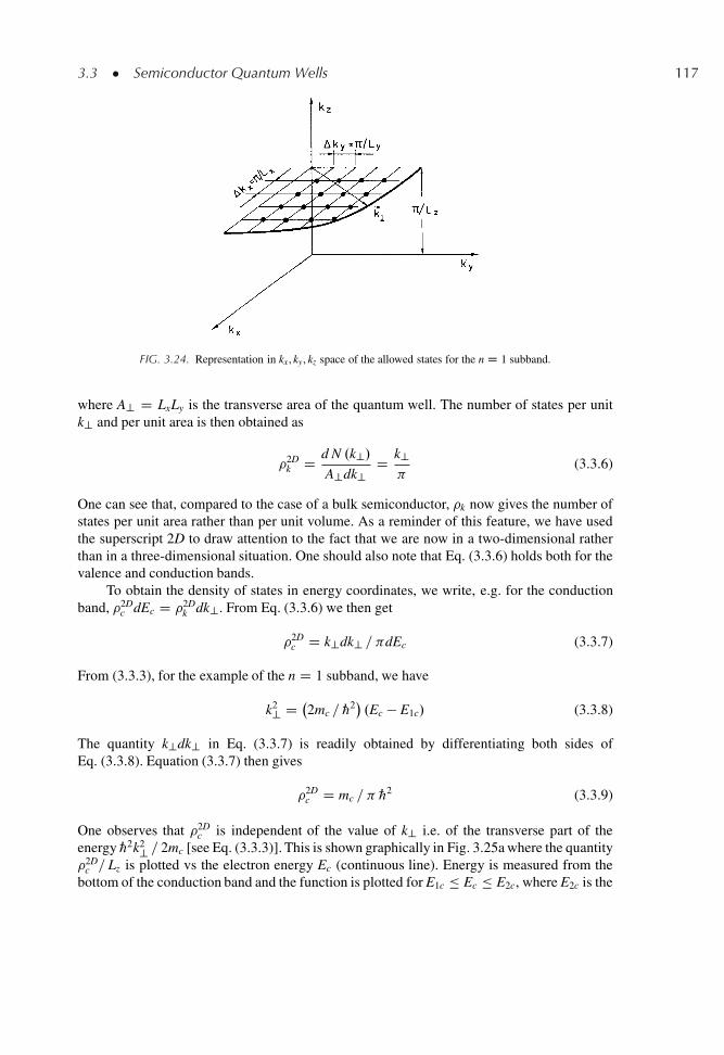
3.3 � Semiconductor Quantum Wells 117
FIG. 3.24. Representation in kx, ky, kz space of the allowed states for the n D 1 subband.
where A? D LxLy is the transverse area of the quantum well. The number of states per unitk? and per unit area is then obtained as
�2Dk D d N .k?/
A?dk?D k?
(3.3.6)
One can see that, compared to the case of a bulk semiconductor, �k now gives the number ofstates per unit area rather than per unit volume. As a reminder of this feature, we have usedthe superscript 2D to draw attention to the fact that we are now in a two-dimensional ratherthan in a three-dimensional situation. One should also note that Eq. (3.3.6) holds both for thevalence and conduction bands.
To obtain the density of states in energy coordinates, we write, e.g. for the conductionband, �2D
c dEc D �2Dk dk?. From Eq. (3.3.6) we then get
�2Dc D k?dk? = dEc (3.3.7)
From (3.3.3), for the example of the n D 1 subband, we have
k2? D 2mc = „2� .Ec � E1c/ (3.3.8)
The quantity k?dk? in Eq. (3.3.7) is readily obtained by differentiating both sides ofEq. (3.3.8). Equation (3.3.7) then gives
�2Dc D mc = „2 (3.3.9)
One observes that �2Dc is independent of the value of k? i.e. of the transverse part of the
energy „2k2? = 2mc [see Eq. (3.3.3)]. This is shown graphically in Fig. 3.25a where the quantity�2D
c = Lz is plotted vs the electron energy Ec (continuous line). Energy is measured from thebottom of the conduction band and the function is plotted for E1c Ec E2c, where E2c is the
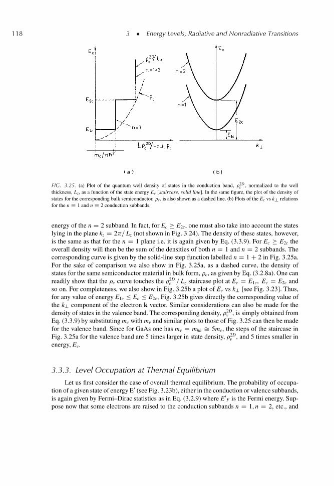
118 3 � Energy Levels, Radiative and Nonradiative Transitions
FIG. 3.25. (a) Plot of the quantum well density of states in the conduction band, �2Dc , normalized to the well
thickness, Lz, as a function of the state energy Ec [staircase, solid line]. In the same figure, the plot of the density ofstates for the corresponding bulk semiconductor, �c, is also shown as a dashed line. (b) Plots of the Ec vs k? relationsfor the n D 1 and n D 2 conduction subbands.
energy of the n D 2 subband. In fact, for Ec E2c, one must also take into account the stateslying in the plane kz D 2 = Lz (not shown in Fig. 3.24). The density of these states, however,is the same as that for the n D 1 plane i.e. it is again given by Eq. (3.3.9). For Ec E2c theoverall density will then be the sum of the densities of both n D 1 and n D 2 subbands. Thecorresponding curve is given by the solid-line step function labelled n D 1 C 2 in Fig. 3.25a.For the sake of comparison we also show in Fig. 3.25a, as a dashed curve, the density ofstates for the same semiconductor material in bulk form, �c, as given by Eq. (3.2.8a). One canreadily show that the �c curve touches the �2D
c = Lz staircase plot at Ec D E1c, Ec D E2c andso on. For completeness, we also show in Fig. 3.25b a plot of Ec vs k? [see Fig. 3.23]. Thus,for any value of energy E1c Ec E2c, Fig. 3.25b gives directly the corresponding value ofthe k? component of the electron k vector. Similar considerations can also be made for thedensity of states in the valence band. The corresponding density, �2D
v , is simply obtained fromEq. (3.3.9) by substituting mc with mv and similar plots to those of Fig. 3.25 can then be madefor the valence band. Since for GaAs one has mv D mhh Š 5mc, the steps of the staircase inFig. 3.25a for the valence band are 5 times larger in state density, �2D
v , and 5 times smaller inenergy, Ev.
3.3.3. Level Occupation at Thermal Equilibrium
Let us first consider the case of overall thermal equilibrium. The probability of occupa-tion of a given state of energy E0 (see Fig. 3.23b), either in the conduction or valence subbands,is again given by Fermi–Dirac statistics as in Eq. (3.2.9) where E0
F is the Fermi energy. Sup-pose now that some electrons are raised to the conduction subbands n D 1, n D 2, etc., and
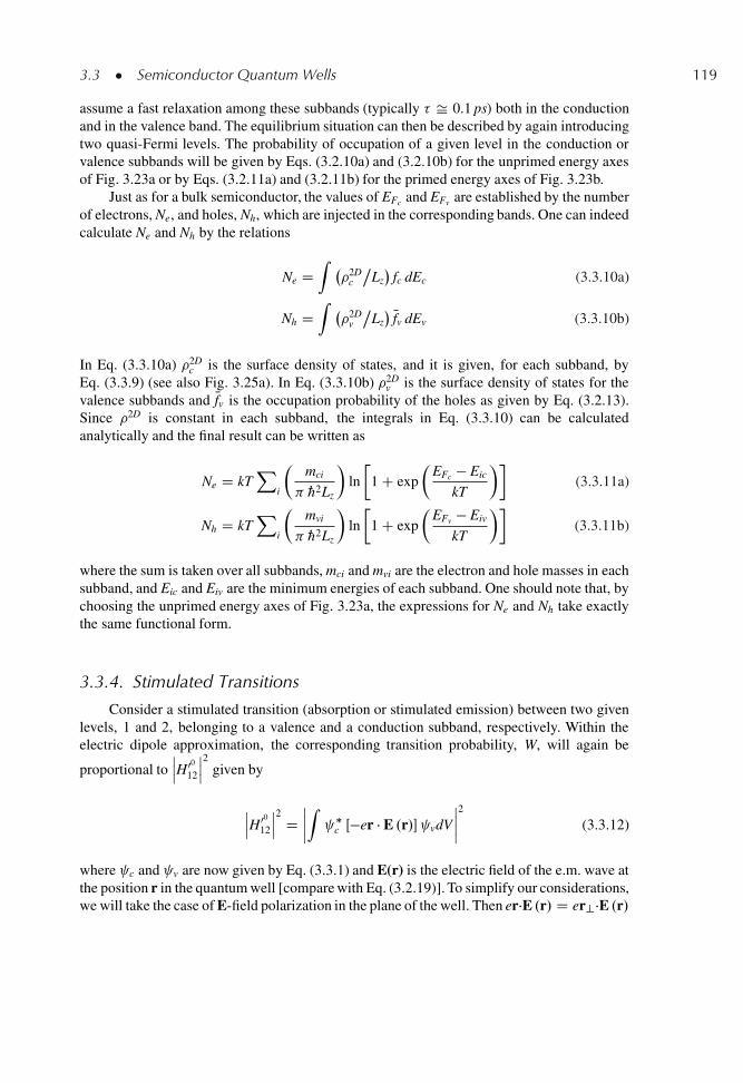
3.3 � Semiconductor Quantum Wells 119
assume a fast relaxation among these subbands (typically � Š 0.1 ps) both in the conductionand in the valence band. The equilibrium situation can then be described by again introducingtwo quasi-Fermi levels. The probability of occupation of a given level in the conduction orvalence subbands will be given by Eqs. (3.2.10a) and (3.2.10b) for the unprimed energy axesof Fig. 3.23a or by Eqs. (3.2.11a) and (3.2.11b) for the primed energy axes of Fig. 3.23b.
Just as for a bulk semiconductor, the values of EFc and EFv are established by the numberof electrons, Ne, and holes, Nh, which are injected in the corresponding bands. One can indeedcalculate Ne and Nh by the relations
Ne DZ
�2Dc
ıLz�
fc dEc (3.3.10a)
Nh DZ
�2Dv
ıLz� Nfv dEv (3.3.10b)
In Eq. (3.3.10a) �2Dc is the surface density of states, and it is given, for each subband, by
Eq. (3.3.9) (see also Fig. 3.25a). In Eq. (3.3.10b) �2Dv is the surface density of states for the
valence subbands and Nfv is the occupation probability of the holes as given by Eq. (3.2.13).Since �2D is constant in each subband, the integrals in Eq. (3.3.10) can be calculatedanalytically and the final result can be written as
Ne D kTX
i
�mci
„2Lz
�ln
�1 C exp
�EFc � Eic
kT
��(3.3.11a)
Nh D kTX
i
�mvi
„2Lz
�ln
�1 C exp
�EFv � Eiv
kT
��(3.3.11b)
where the sum is taken over all subbands, mci and mvi are the electron and hole masses in eachsubband, and Eic and Eiv are the minimum energies of each subband. One should note that, bychoosing the unprimed energy axes of Fig. 3.23a, the expressions for Ne and Nh take exactlythe same functional form.
3.3.4. Stimulated Transitions
Consider a stimulated transition (absorption or stimulated emission) between two givenlevels, 1 and 2, belonging to a valence and a conduction subband, respectively. Within theelectric dipole approximation, the corresponding transition probability, W, will again be
proportional toˇH00
12
ˇ2given by
ˇH00
12
ˇ2 DˇˇZ �
c Œ�er � E .r/� vdV
ˇˇ2
(3.3.12)
where c and v are now given by Eq. (3.3.1) and E(r) is the electric field of the e.m. wave atthe position r in the quantum well [compare with Eq. (3.2.19)]. To simplify our considerations,we will take the case of E-field polarization in the plane of the well. Then er�E .r/ D er?�E .r/
120 3 � Energy Levels, Radiative and Nonradiative Transitions
Example 3.10. Calculation of the Quasi-Fermi energiesfor a GaAs/AlGaAs quantum well. We will take mci Dmc D 0.067 m0 and mvi D 0.46 m0, i.e. we will assumethat the masses are the same as those of the bulk materialand we will neglect the contribution of the light holes.We will also assume Lz D 10 nm and T D 300 K. FromEq. (3.3.11) one readily obtains the two plots of concen-tration N vs .EF � E1/=kT, both for electrons and holes,shown in Fig. 3.26. From this figure, the position of thequasi-Fermi levels for a given injection, N, of electronsand holes, can be readily obtained.
where r? is the component of the r vectorin the well plane. We further notice that thewell thickness is much smaller than the wave-length of light. Hence E(r) can be taken to beconstant along the direction z orthogonal tothe well and we can thus write E D E.r?/i.e. a function of only the transverse coordi-nate r?. It then follows that er?�E .r/ reducesto er? � E .r?/ and Eq. (3.3.12) can be splitinto two integrals, one over the orthogonalcoordinates, x and y, and the other over thelongitudinal one z, viz
ˇˇH00
12
ˇˇ2 D
ˇˇZ
u�c .r?/ e�jkc? �r?
��er? � Eoejkopt�r?
uv.r?/ejkv?�r? dxdy
ˇˇ2
� (3.3.13)
�ˇˇZ
sin .nc z=Lz/ sin .nv z=Lz/dz
ˇˇ2
As in the case of a bulk semiconductor, the integral over the transverse coordinates can beshown to vanish unless kv? C kopt D kc?. Since again
ˇkopt
ˇ<< .jkv?j , jkc?j/ we obtain the
selection rule [compare with Eq. (3.2.22)]
kc? D kv? (3.3.14)
Thus the k-conservation rule still holds for the transverse component, k?, and this impliesthat transitions must occur vertically in Fig. 3.23. From the second integral of the right hand
FIG. 3.26. Plots of the normalized difference between the quasi-Fermi energy, EF , and the energy of the n D 1subband, E1, vs density of injected carriers, for both electrons and holes, in a 10 nm GaAs/AlGaAs quantum well.
3.3 � Semiconductor Quantum Wells 121
side of Eq. (3.3.13), since nc and nv are positive integers we get the selection rule for thequantum number n as
�n D nc � nv D 0 (3.3.15)
which shows that transitions can only occur between two subbands, one in the conduction andthe other in the valence band, with the same quantum number n. One should finally note thatspin is not involved in the interaction Hamiltonian e r � E, i.e. the e.m. wave does not interactwith spin. This implies that spin cannot change in the transition i.e. that
�S D 0 (3.3.16)
where S is the spin quantum number of the electron involved.It should be noted that the selection rules Eqs. (3.3.14), (3.3.15), and (3.3.16) have been
derived subject to the simplifying assumptions that the E-field be polarized in the plane of thewell. It can be shown however.13/ that the same rules hold in general and, from now on, theserules will be used extensively.
3.3.5. Absorption and Gain Coefficients
To calculate absorption obeying k?-conservation rule it is appropriate to first introducethe joint density of transitions or joint density of states, �2D
Jk , such that �2DJk dk? gives the
number of available transitions or the number of coupled states per unit area, with k? rangingbetween k? and k? C dk?. Since transitions can only occur vertically in Fig. 3.23 and since�S D 0, this number is also equal to the number of states in either the valence or conductionbands within the same elemental interval dk?. Thus we get
�2DJk D �2D
k D k? = (3.3.17)
where Eq. (3.3.6) has been used. Consider now two given energy levels of energy E02 and E0
1
belonging to e.g. the n D 1 subbands of the conduction and valence band respectively. FromFig. 3.23b and Eq. (3.3.3), the energy difference, E0 D h�0 D E0
2 � E0, is seen to be given by
E0 D Eg C „2k2?
2 mrC�E1 (3.3.18)
where mr is the reduced mass and�E1 D E1c C E1v. If we now introduce the density of statesin the E0 coordinate, �2D
JE0, we can write
�2DJE0
dE0 D �2DJk dk? D k?dk? = (3.3.19)
where Eq. (3.3.17) has been used. The quantity k?dk? is then obtained by differentiating bothsides of Eq. (3.3.18). From Eq. (3.3.19) we then get
�2DJE0
D mr = „2 (3.3.20)
122 3 � Energy Levels, Radiative and Nonradiative Transitions
If we now define the density of states with respect to the transition frequency coordinate�0, �J�0 , then, since we must have again �2D
J�0d�0 D �2D
JE0dE0, we get from Eq. (3.3.20)
�2DJ�0
D 4 mr = h (3.3.21)
The calculation of the overall absorption at the frequency � of the incoming e.m. wavecan be made in the same way as the calculation performed for bulk material, i.e. throughEqs. (3.2.30)–(3.2.32), provided we substitute �J .�0/with
�2D
J�0
ıLz�
which is the joint densityof states for our case. Again assuming infinitely narrow transitions between any two states,the absorption coefficient for the n D 1 ! n D 1 quantum well transition is readily obtainedfrom Eqs. (3.2.34) and (3.2.35) as
˛QW D�
2 2�
n"0ch
��2
3
��2D
J�
Lz
� �fvE0
1
� � fcE0
2
�(3.3.22)
where E01 and E0
2 are now the energies of the two levels whose transition frequency is equal to�. Under the k?-conservation rule, E0
2 and E01 can readily be obtained from Fig. 3.23a,b with
the help of Eq. (3.3.3), by letting �0 D �.
Example 3.11. Calculation of the absorption coefficient in a GaAs/AlGaAs quantum well. We will firstconsider the case of T D 0 K. In this case all valence subbands are full, all conduction subbands are emptyand we have fv
E0
1
� D 1 and fcE0
2
� D 0. The absorption coefficient then has its maximum value, given by
˛maxQW D
�2 2�
n"0ch
��2
3
�2DJ�
Lz(3.3.23)
whose dependence upon the photon energy is essentially determined by �2DJ� . The absorption coefficient vs
the difference,E � Eg
�, between the photon energy and the gap energy as calculated from Eq. (3.3.23)
for a Lz D 10 nm quantum well is shown in Fig. 3.27. According to Fig. 3.25a, �2DJ� is seen to be zero for
a photon energy E < Eg C E1c C E1v D Eg C�E1. No absorption is thus expected forE � Eg
�< �E1.
Assuming again mc D 0.067 m0 and mv D 0.46 m0, from example 3.8 we get�E1 D E1cCE1v Š 65 meV.For�E1 .E � Eg/ �E2, where�E2 D E2c C E2v, �2D
J� is given by Eq. (3.3.21), with �0 D �, and theabsorption coefficient has a constant value given by
˛QW D 8 3
n"0�h2
��2
3
�mr
Lz(3.3.24)
where � D c=� According to example 3.5, we will take��2ı
31=2 D 0.68 � 10�25 C � m, mr D
5.37 � 10�32 Kg, n D 3.64 and � D 833 nm. From Eq. (3.3.24) we then get ˛QW D 5, 250 cm�1. ForE � Eg
� �E2, transitions between the n D 2 subbands also occur, the joint density of states doubles(see also Fig. 3.25a) and the absorption coefficient will also double. Note that, since E2c D 4E1c andE2v D 4E1v, one has �E2 D 4�E1 D 260 meV D 260 meV (one can now compare Fig. 3.27 withFig. 3.16).
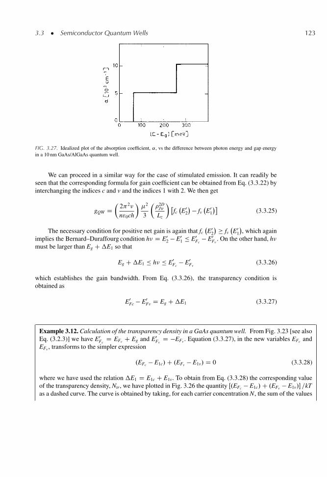
3.3 � Semiconductor Quantum Wells 123
FIG. 3.27. Idealized plot of the absorption coefficient, ˛, vs the difference between photon energy and gap energyin a 10 nm GaAs/AlGaAs quantum well.
We can proceed in a similar way for the case of stimulated emission. It can readily beseen that the corresponding formula for gain coefficient can be obtained from Eq. (3.3.22) byinterchanging the indices c and v and the indices 1 with 2. We then get
gQW D�
2 2�
n"0ch
��2
3
��2D
J�
Lz
� �fcE0
2
� � fvE0
1
�(3.3.25)
The necessary condition for positive net gain is again that fcE0
2
� fvE0
1
�, which again
implies the Bernard–Duraffourg condition h� D E02 � E0
1 E0Fc
� E0Fv
. On the other hand, h�must be larger than Eg C�E1 so that
Eg C�E1 h� E0Fc
� E0Fv
(3.3.26)
which establishes the gain bandwidth. From Eq. (3.3.26), the transparency condition isobtained as
E0Fc � E0
Fv D Eg C�E1 (3.3.27)
Example 3.12. Calculation of the transparency density in a GaAs quantum well. From Fig. 3.23 [see alsoEq. (3.2.3)] we have E0
FcD EFc C Eg and E0
FvD �EFv . Equation (3.3.27), in the new variables EFc and
EFv , transforms to the simpler expression
.EFc � E1c/C .EFv � E1v/ D 0 (3.3.28)
where we have used the relation �E1 D E1c C E1v. To obtain from Eq. (3.3.28) the corresponding valueof the transparency density, Ntr , we have plotted in Fig. 3.26 the quantity Œ.EFc � E1c/C .EFv � E1v/� =kTas a dashed curve. The curve is obtained by taking, for each carrier concentration N, the sum of the values
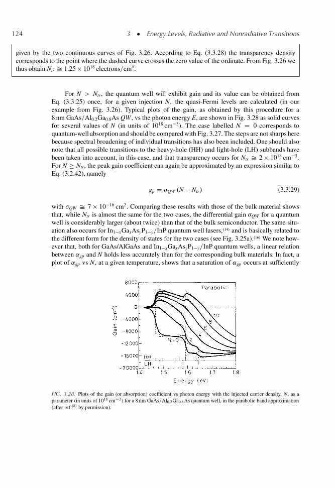
124 3 � Energy Levels, Radiative and Nonradiative Transitions
given by the two continuous curves of Fig. 3.26. According to Eq. (3.3.28) the transparency densitycorresponds to the point where the dashed curve crosses the zero value of the ordinate. From Fig. 3.26 wethus obtain Ntr Š 1.25 � 1018 electrons=cm3.
For N > Ntr, the quantum well will exhibit gain and its value can be obtained fromEq. (3.3.25) once, for a given injection N, the quasi-Fermi levels are calculated (in ourexample from Fig. 3.26). Typical plots of the gain, as obtained by this procedure for a8 nm GaAs=Al0.2Ga0.8As QW, vs the photon energy E, are shown in Fig. 3.28 as solid curvesfor several values of N (in units of 1018 cm�3). The case labelled N D 0 corresponds toquantum-well absorption and should be compared with Fig. 3.27. The steps are not sharps herebecause spectral broadening of individual transitions has also been included. One should alsonote that all possible transitions to the heavy-hole (HH) and light-hole (LH) subbands havebeen taken into account, in this case, and that transparency occurs for Ntr Š 2 � 1018 cm�3.For N Ntr, the peak gain coefficient can again be approximated by an expression similar toEq. (3.2.42), namely
gp D �QW .N � Ntr/ (3.3.29)
with �QW Š 7 � 10�16 cm2. Comparing these results with those of the bulk material showsthat, while Ntr is almost the same for the two cases, the differential gain �QW for a quantumwell is considerably larger (about twice) than that of the bulk semiconductor. The same situ-ation also occurs for In1�xGaxAsyP1�y=InP quantum well lasers,.14/ and is basically related tothe different form for the density of states for the two cases (see Fig. 3.25a)..16/ We note how-ever that, both for GaAs/AlGaAs and In1�xGaxAsyP1�y=InP quantum wells, a linear relationbetween ˛gp and N holds less accurately than for the corresponding bulk materials. In fact, aplot of ˛gp vs N, at a given temperature, shows that a saturation of ˛gp occurs at sufficiently
FIG. 3.28. Plots of the gain (or absorption) coefficient vs photon energy with the injected carrier density, N, as aparameter (in units of 1018 cm�3) for a 8 nm GaAs=Al0.2Ga0.8As quantum well, in the parabolic band approximation(after ref..8/ by permission).
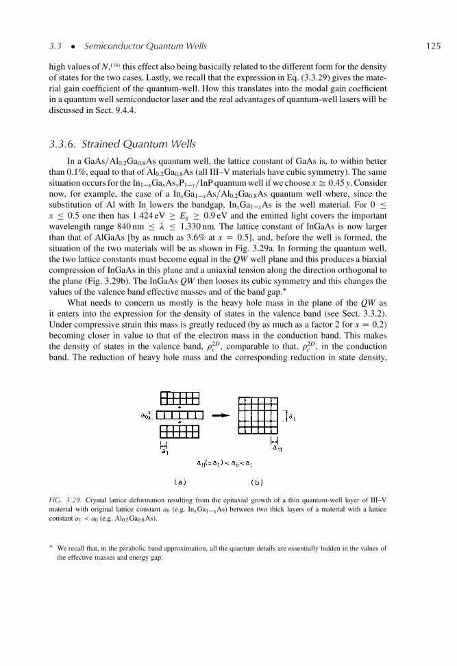
3.3 � Semiconductor Quantum Wells 125
high values of N,.14/ this effect also being basically related to the different form for the densityof states for the two cases. Lastly, we recall that the expression in Eq. (3.3.29) gives the mate-rial gain coefficient of the quantum-well. How this translates into the modal gain coefficientin a quantum well semiconductor laser and the real advantages of quantum-well lasers will bediscussed in Sect. 9.4.4.
3.3.6. Strained Quantum Wells
In a GaAs=Al0.2Ga0.8As quantum well, the lattice constant of GaAs is, to within betterthan 0.1%, equal to that of Al0.2Ga0.8As (all III–V materials have cubic symmetry). The samesituation occurs for the In1�xGaxAsyP1�y=InP quantum well if we choose x Š 0.45 y. Considernow, for example, the case of a InxGa1�xAs=Al0.2Ga0.8As quantum well where, since thesubstitution of Al with In lowers the bandgap, InxGa1�xAs is the well material. For 0 x 0.5 one then has 1.424 eV Eg 0.9 eV and the emitted light covers the importantwavelength range 840 nm � 1,330 nm. The lattice constant of InGaAs is now largerthan that of AlGaAs [by as much as 3.6% at x D 0.5], and, before the well is formed, thesituation of the two materials will be as shown in Fig. 3.29a. In forming the quantum well,the two lattice constants must become equal in the QW well plane and this produces a biaxialcompression of InGaAs in this plane and a uniaxial tension along the direction orthogonal tothe plane (Fig. 3.29b). The InGaAs QW then looses its cubic symmetry and this changes thevalues of the valence band effective masses and of the band gap.�
What needs to concern us mostly is the heavy hole mass in the plane of the QW asit enters into the expression for the density of states in the valence band (see Sect. 3.3.2).Under compressive strain this mass is greatly reduced (by as much as a factor 2 for x D 0.2)becoming closer in value to that of the electron mass in the conduction band. This makesthe density of states in the valence band, �2D
v , comparable to that, �2Dc , in the conduction
band. The reduction of heavy hole mass and the corresponding reduction in state density,
FIG. 3.29. Crystal lattice deformation resulting from the epitaxial growth of a thin quantum-well layer of III–Vmaterial with original lattice constant a0 (e.g. InxGa1�xAs) between two thick layers of a material with a latticeconstant a1 < a0 (e.g. Al0.2Ga0.8As).
� We recall that, in the parabolic band approximation, all the quantum details are essentially hidden in the values ofthe effective masses and energy gap.
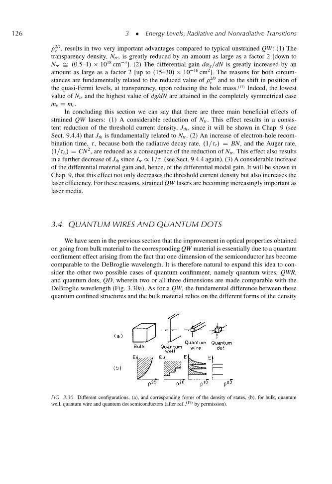
126 3 � Energy Levels, Radiative and Nonradiative Transitions
�2Dv , results in two very important advantages compared to typical unstrained QW: (1) The
transparency density, Ntr , is greatly reduced by an amount as large as a factor 2 [down toNtr Š .0.5–1/ � 1018 cm�3]. (2) The differential gain d˛g=dN is greatly increased by anamount as large as a factor 2 [up to .15–30/ � 10�16 cm2]. The reasons for both circum-stances are fundamentally related to the reduced value of �2D
v and to the shift in position ofthe quasi-Fermi levels, at transparency, upon reducing the hole mass..17/ Indeed, the lowestvalue of Ntr and the highest value of dg/dN are attained in the completely symmetrical casemv D mc.
In concluding this section we can say that there are three main beneficial effects ofstrained QW lasers: (1) A considerable reduction of Ntr. This effect results in a consis-tent reduction of the threshold current density, Jth, since it will be shown in Chap. 9 (seeSect. 9.4.4) that Jth is fundamentally related to Ntr. (2) An increase of electron-hole recom-bination time, � , because both the radiative decay rate, .1=�r/ D BN, and the Auger rate,.1=�A/ D CN2, are reduced as a consequence of the reduction of Ntr. This effect also resultsin a further decrease of Jth since Jtr / 1=� . (see Sect. 9.4.4 again). (3) A considerable increaseof the differential material gain and, hence, of the differential modal gain. It will be shown inChap. 9, that this effect not only decreases the threshold current density but also increases thelaser efficiency. For these reasons, strained QW lasers are becoming increasingly important aslaser media.
3.4. QUANTUM WIRES AND QUANTUM DOTS
We have seen in the previous section that the improvement in optical properties obtainedon going from bulk material to the corresponding QW material is essentially due to a quantumconfinment effect arising from the fact that one dimension of the semiconductor has becomecomparable to the DeBroglie wavelength. It is therefore natural to expand this idea to con-sider the other two possible cases of quantum confinment, namely quantum wires, QWR,and quantum dots, QD, wherein two or all three dimensions are made comparable with theDeBroglie wavelength (Fig. 3.30a). As for a QW, the fundamental difference between thesequantum confined structures and the bulk material relies on the different forms of the density
FIG. 3.30. Different configurations, (a), and corresponding forms of the density of states, (b), for bulk, quantumwell, quantum wire and quantum dot semiconductors (after ref.,.19/ by permission).
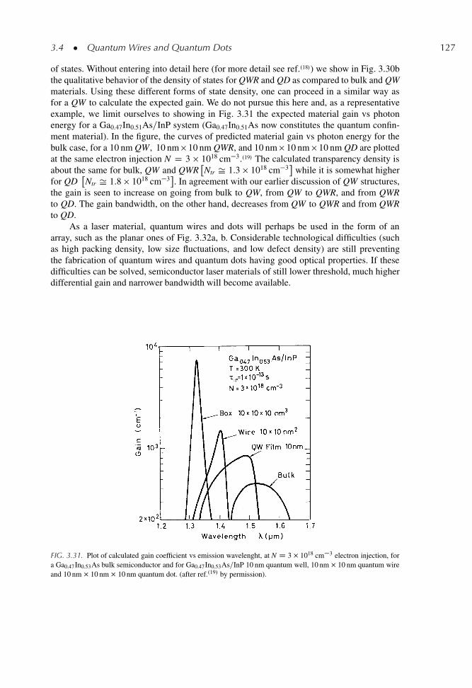
3.4 � Quantum Wires and Quantum Dots 127
of states. Without entering into detail here (for more detail see ref..18/) we show in Fig. 3.30bthe qualitative behavior of the density of states for QWR and QD as compared to bulk and QWmaterials. Using these different forms of state density, one can proceed in a similar way asfor a QW to calculate the expected gain. We do not pursue this here and, as a representativeexample, we limit ourselves to showing in Fig. 3.31 the expected material gain vs photonenergy for a Ga0.47In0.51As=InP system (Ga0.47In0.51As now constitutes the quantum confin-ment material). In the figure, the curves of predicted material gain vs photon energy for thebulk case, for a 10 nm QW, 10 nm � 10 nm QWR, and 10 nm � 10 nm � 10 nm QD are plottedat the same electron injection N D 3 � 1018 cm�3..19/ The calculated transparency density isabout the same for bulk, QW and QWR
�Ntr Š 1.3 � 1018 cm�3
while it is somewhat higher
for QD�Ntr Š 1.8 � 1018 cm�3
. In agreement with our earlier discussion of QW structures,
the gain is seen to increase on going from bulk to QW, from QW to QWR, and from QWRto QD. The gain bandwidth, on the other hand, decreases from QW to QWR and from QWRto QD.
As a laser material, quantum wires and dots will perhaps be used in the form of anarray, such as the planar ones of Fig. 3.32a, b. Considerable technological difficulties (suchas high packing density, low size fluctuations, and low defect density) are still preventingthe fabrication of quantum wires and quantum dots having good optical properties. If thesedifficulties can be solved, semiconductor laser materials of still lower threshold, much higherdifferential gain and narrower bandwidth will become available.
FIG. 3.31. Plot of calculated gain coefficient vs emission wavelenght, at N D 3 1018 cm�3 electron injection, fora Ga0.47In0.53As bulk semiconductor and for Ga0.47In0.53As=InP 10 nm quantum well, 10 nm 10 nm quantum wireand 10 nm 10 nm 10 nm quantum dot. (after ref..19/ by permission).
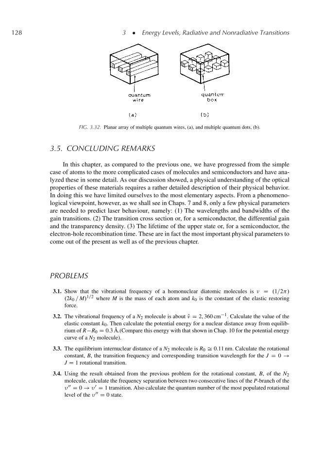
128 3 � Energy Levels, Radiative and Nonradiative Transitions
FIG. 3.32. Planar array of multiple quantum wires, (a), and multiple quantum dots, (b).
3.5. CONCLUDING REMARKS
In this chapter, as compared to the previous one, we have progressed from the simplecase of atoms to the more complicated cases of molecules and semiconductors and have ana-lyzed these in some detail. As our discussion showed, a physical understanding of the opticalproperties of these materials requires a rather detailed description of their physical behavior.In doing this we have limited ourselves to the most elementary aspects. From a phenomeno-logical viewpoint, however, as we shall see in Chaps. 7 and 8, only a few physical parametersare needed to predict laser behaviour, namely: (1) The wavelengths and bandwidths of thegain transitions. (2) The transition cross section or, for a semiconductor, the differential gainand the transparency density. (3) The lifetime of the upper state or, for a semiconductor, theelectron-hole recombination time. These are in fact the most important physical parameters tocome out of the present as well as of the previous chapter.
PROBLEMS
3.1. Show that the vibrational frequency of a homonuclear diatomic molecules is � D .1=2 /.2k0 =M/1=2 where M is the mass of each atom and k0 is the constant of the elastic restoringforce.
3.2. The vibrational frequency of a N2 molecule is about Q� D 2, 360 cm�1. Calculate the value of theelastic constant k0. Then calculate the potential energy for a nuclear distance away from equilib-rium of R�R0 D 0.3 A.(Compare this energy with that shown in Chap. 10 for the potential energycurve of a N2 molecule).
3.3. The equilibrium internuclear distance of a N2 molecule is R0 Š 0.11 nm. Calculate the rotationalconstant, B, the transition frequency and corresponding transition wavelength for the J D 0 !J D 1 rotational transition.
3.4. Using the result obtained from the previous problem for the rotational constant, B, of the N2molecule, calculate the frequency separation between two consecutive lines of the P-branch of the� 00 D 0 ! � 0 D 1 transition. Also calculate the quantum number of the most populated rotationallevel of the � 00 D 0 state.

References 129
3.5. The rotational constant of a CO2 molecule in its 00ı1 vibrational level is B D 0.37 cm�1. Assum-ing the same value for the rotational constant of the 10ı0 level, calculate the P-branch andR-branch spectrum at T D 450 K of the 00ı1 ! 10ı0 transition [remember that only rotationallevels of the 00ı1 upper state of even J number can partecipate in the transition].
3.6. Assuming that the rotational constant of the ground vibrational state of a CO2 molecule is B D0.37 cm�1, i.e. it is equal to that of the .00ı1/ state, calculate the equilibrium distance R0 betweenthe carbon and oxygen atoms.
3.7. From the condition fcE0
2� fv
E0
1�
prove the Bernard–Duraffourg relation E0Fc � E0
Fv h�.
3.8. With the help of Fig. 3.15b calculate for GaAs: (a) The values of EFc and EFv at N D 1.6 �1018 cm�3 carrier injection. (a) The overall gain bandwidth at the same injection.
3.9. In the energy reference system of Fig. 3.9a calculate, for GaAs, the energies, E2 and E1, of theupper and lower laser levels for a transition energy exceeding the bandgap energy by 0.45 kT.
3.10. For a bulk GaAs semiconductor, with the help of Fig. 3.16, calculate the expected gain at a photonenergy exceeding the badgap energy by 0.45 kT and for a carrier injection of N D 1.6�1018 cm�3.
3.11. Assuming that the peak gain in a bulk GaAs semiconductor at a carrier injection N D 1.6 �1018 cm�3 occurs at a photon energy exceeding the gap energy by 0.45 kT and using some of theresults obtained in problems 3.9, 3.10 and 3.11, calculate the differential gain � D d˛g=dN.
3.12. With the help of Fig. 3.15a, plot on the same figure the quantities EFc=kT , EFv=kT , andEFc C EFv
�=kT vs the concentration, N, of electrons and holes for bulk InGaAsP at � D
1, 300 nm. From these plots then calculate the transparency density Ntr and, from a compari-son of this figure with Fig. 3.15b, explain why Ntr is, in this case, somewhat smaller than in theGaAs case. From the same plots calculate also the overall gain bandwidth and the values of EFc
and EFv at N D 1.6 � 1018 cm�3 carrier injection. On assuming that the maximum gain occurs atan energy of �E D 0.65 kT above band gap energy, calculate the corresponding wavelength.
3.13. For a 10 nm GaAs quantum well calculate from Fig. 3.26 the overall bandwidth of the gain curveand the values of the quasi-Fermi levels for an injected carrier density of N D 2 � 1018 cm�3. Inthe .E-Eg/ reference axis of Fig. 3.27 find the energy interval in which positive gain occurs.
3.14. Calculate how the first step of Fig. 3.27 at .E-Eg/ Š 65 meV needs to be modified if a Lorentzianlineshape with a dephasing time �c D 0.1 ps is assumed for each transition from an upper level inthe first conduction subband to a lower level in the first valence subband.
References
1. G. Herzberg, Spectra of Diatomic Molecules (D. Van Nostrand Company, Princeton NJ, 1950).
2. G. Herzberg, Molecular Spectra and Molecular Structure: Infrared and Raman Spectra of Polyatomic Molecules,(D. Van Nostrand Company, Princeton NJ, 1968), p. 122, Fig. 51.
3. G.B. Agrawal and N.K. Dutta, Long Wavelength Semiconductor Lasers (Chapman and Hall, New York, 1986).
4. C. Kittel, Introduction to Solid State Physics, 6th Ed. (Wiley, New York, 1986)
5. R.H. Yan, S.W. Corzine, L.A. Coldren, and I Suemune, Correction for the Expression for Gain in GaAs, IEEE J.Quantum Electron QE–26, 213–216 (1990).
6. M.G. Bernard and G. Duraffourg, Laser Conditions in Semiconductors, Phys. Status Solidi 1, 699 (1961).
7. Ref. [3] Chap. 3

130 3 � Energy Levels, Radiative and Nonradiative Transitions
8. S.W. Corzine, R.H. Yan, and L.A. Coldren, Optical Gain in III-V Bulk and Quantum well Semiconductors, In:Quantum Well Lasers ed. by P.S. Zory (Academic, San Diego, CA, 1993) Chap. 1.
9. G.H.B. Thompson, Physics of Semiconductor Lasers Devices (Wiley, New York, 1980) sect. 2.5.2.10. Ref. [9] sect. 2.4.2.11. Ref. [8] Fig. 2.14.12. Ref. [3] sect. 3.3.13. Ref. [8] sect. 3.1.14. Ref. [3] Chap. 9.15. A. Yariv, Quantum Electronics third ed. (Wiley, New York, 1989) sect. 11.216. Ref. [8], sect. 4.1.17. Ref. [8] Fig. 6.18. E. Kapon, Quantum Wire Semiconductor Lasers, In: Quantum Well Lasers, ed. by P.S. Zory (Academic, San
Diego, CA, 1983) Chap. 10.19. M. Asada, Y. Miyamoto, and Y. Suematsu, Gain and Threshold of Three-Dimensional Quantum-Box Lasers,
IEEE J. Quantum Electron QE–22, 1915–1921 (1986).20. P.K. Cheo, CO2 Lasers, In: Lasers Vol. 3, Eds. A.K. Levine and A. DeMaria (Marcel Dekker, New York, 1971).
4
Ray and Wave PropagationThrough Optical Media
4.1. INTRODUCTION
Before beginning a detailed discussion on optical resonators, which is to be the subjectof the next Chapter, we introduce in this Chapter a few topics from geometrical and waveoptics. The aim is to introduce some subjects that are not usually covered in elementary opticstexts and that constitute a very useful background for the topics to be considered in nextchapter. Thus, in particular, the matrix formulation of geometrical optics within the paraxial-ray approximation and wave propagation within the paraxial-wave approximation, leading tothe ideas of Gaussian beam propagation, will be discussed here. Situations involving multipleinterference such as in a multilayer dielectric coating or in a Fabry-Perot interferometer willalso be considered.
4.2. MATRIX FORMULATION OF GEOMETRICAL OPTICS.1/
Consider a ray of light that is either transmitted by or reflected from an optical elementwhich has reciprocal and polarization-independent behavior (e.g. a lens or a mirror). Let z bethe optical axis of this element (e.g. the line passing through the centers of curvature of thetwo spherical surfaces of the lens). Assume that the ray is traveling approximately along the zdirection in a plane containing the optical axis. The ray vector r1 at a given input plane z D z1
of the optical element (Fig. 4.1) can be characterized by two parameters, namely, its radialdisplacement r.z1/ from the z axis and its angular displacement 1. Likewise, the ray-vectorr2 at a given output plane z D z2 can be characterized by its radial, r2.z2/, and angular 2,displacements. Note that the r-axis is taken to be the same for both input and output raysand oriented as in Fig. 4.1. The sign convention for the angles is that the angle is positive if
O. Svelto, Principles of Lasers,c
131DOI: 10.1007/978-1-4419-1302-9 4, � Springer Science+Business Media LLC 2010
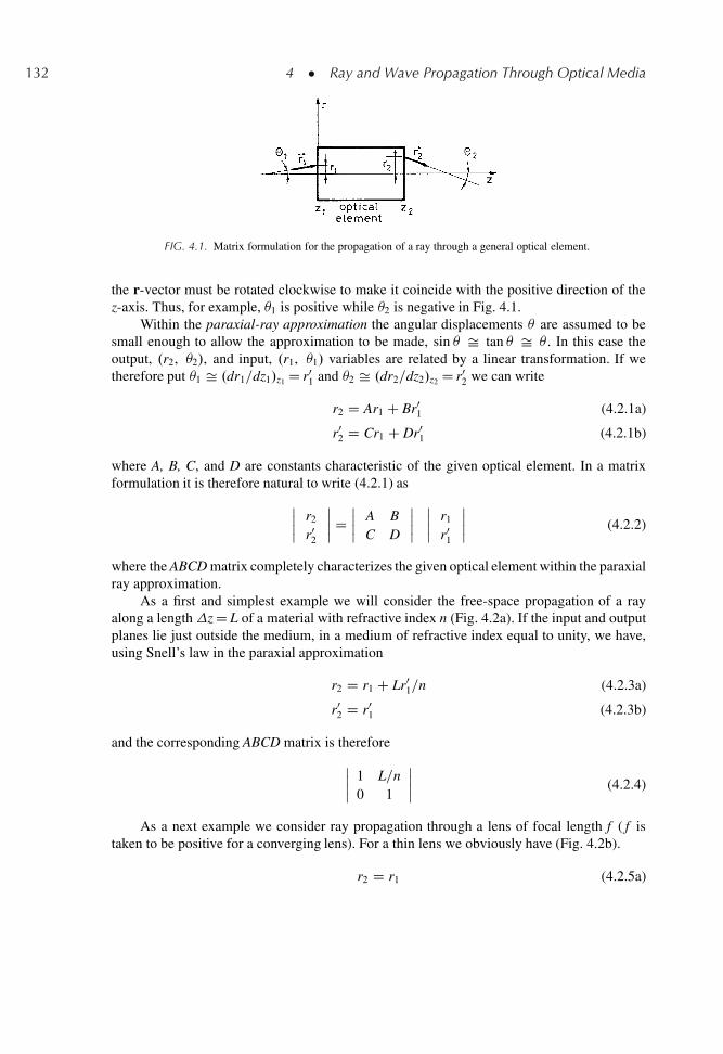
132 4 � Ray and Wave Propagation Through Optical Media
FIG. 4.1. Matrix formulation for the propagation of a ray through a general optical element.
the r-vector must be rotated clockwise to make it coincide with the positive direction of thez-axis. Thus, for example, 1 is positive while 2 is negative in Fig. 4.1.
Within the paraxial-ray approximation the angular displacements are assumed to besmall enough to allow the approximation to be made, sin Š tan Š . In this case theoutput, .r2, 2/, and input, .r1, 1/ variables are related by a linear transformation. If wetherefore put 1 Š .dr1=dz1/z1 D r0
1 and 2 Š .dr2=dz2/z2 D r02 we can write
r2 D Ar1 C Br01 (4.2.1a)
r02 D Cr1 C Dr0
1 (4.2.1b)
where A, B, C, and D are constants characteristic of the given optical element. In a matrixformulation it is therefore natural to write (4.2.1) as
ˇˇ r2
r02
ˇˇ D
ˇˇ A B
C D
ˇˇˇˇ r1
r01
ˇˇ (4.2.2)
where the ABCD matrix completely characterizes the given optical element within the paraxialray approximation.
As a first and simplest example we will consider the free-space propagation of a rayalong a lengthz D L of a material with refractive index n (Fig. 4.2a). If the input and outputplanes lie just outside the medium, in a medium of refractive index equal to unity, we have,using Snell’s law in the paraxial approximation
r2 D r1 C Lr01=n (4.2.3a)
r02 D r0
1 (4.2.3b)
and the corresponding ABCD matrix is therefore
ˇˇ 1 L=n
0 1
ˇˇ (4.2.4)
As a next example we consider ray propagation through a lens of focal length f ( f istaken to be positive for a converging lens). For a thin lens we obviously have (Fig. 4.2b).
r2 D r1 (4.2.5a)
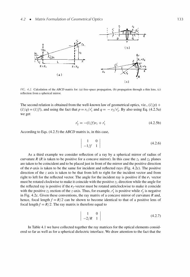
4.2 � Matrix Formulation of Geometrical Optics 133
FIG. 4.2. Calculation of the ABCD matrix for: (a) free-space propagation, (b) propagation through a thin lens, (c)reflection from a spherical mirror.
The second relation is obtained from the well-known law of geometrical optics, viz., .1=p/C.1=q/D .1=f /, and using the fact that p D r1=r0
1 and q D � r2=r02. By also using Eq. (4.2.5a)
we get
r02 D �.1=f /r1 C r0
1 (4.2.5b)
According to Eqs. (4.2.5) the ABCD matrix is, in this case,
ˇˇ 1 0
�1=f 1
ˇˇ (4.2.6)
As a third example we consider reflection of a ray by a spherical mirror of radius ofcurvature R (R is taken to be positive for a concave mirror). In this case the z1 and z2 planesare taken to be coincident and to be placed just in front of the mirror and the positive directionof the r-axis is taken to be the same for incident and reflected rays (Fig. 4.2c). The positivedirection of the z axis is taken to be that from left to right for the incident vector and fromright to left for the reflected vector. The angle for the incident ray is positive if the r1 vectormust be rotated clockwise to make it coincide with the positive z1 direction while the angle forthe reflected ray is positive if the r2-vector must be rotated anticlockwise to make it coincidewith the positive z2 rection of the z-axis. Thus, for example, r0
1 is positive while r02 is negative
in Fig. 4.2c. Given these conventions, the ray matrix of a concave mirror of curvature R and,hence, focal length f D R=2 can be shown to become identical to that of a positive lens offocal length f D R=2. The ray matrix is therefore equal to
ˇˇ 1 0
�2=R 1
ˇˇ (4.2.7)
In Table 4.1 we have collected together the ray matrices for the optical elements consid-ered so far as well as for a spherical dielectric interface. We draw attention to the fact that the
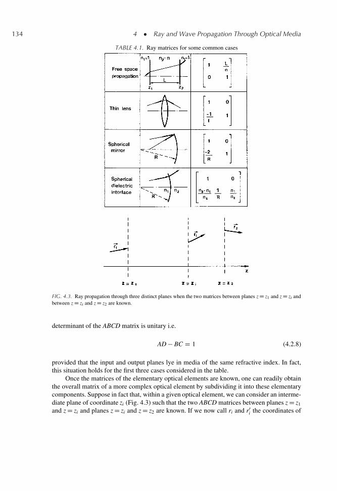
134 4 � Ray and Wave Propagation Through Optical Media
TABLE 4.1. Ray matrices for some common cases
FIG. 4.3. Ray propagation through three distinct planes when the two matrices between planes z D z1 and z D zi andbetween z D zi and z D z2 are known.
determinant of the ABCD matrix is unitary i.e.
AD � BC D 1 (4.2.8)
provided that the input and output planes lye in media of the same refractive index. In fact,this situation holds for the first three cases considered in the table.
Once the matrices of the elementary optical elements are known, one can readily obtainthe overall matrix of a more complex optical element by subdividing it into these elementarycomponents. Suppose in fact that, within a given optical element, we can consider an interme-diate plane of coordinate zi (Fig. 4.3) such that the two ABCD matrices between planes z D z1
and z D zi and planes z D zi and z D z2 are known. If we now call ri and r0i the coordinates of
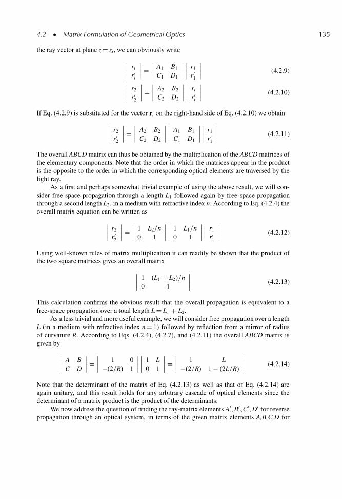
4.2 � Matrix Formulation of Geometrical Optics 135
the ray vector at plane z D zi, we can obviously write
ˇˇ ri
r0i
ˇˇ D
ˇˇ A1 B1
C1 D1
ˇˇˇˇ r1
r01
ˇˇ (4.2.9)
ˇˇ r2
r02
ˇˇ D
ˇˇ A2 B2
C2 D2
ˇˇˇˇ ri
r0i
ˇˇ (4.2.10)
If Eq. (4.2.9) is substituted for the vector ri on the right-hand side of Eq. (4.2.10) we obtain
ˇˇ r2
r02
ˇˇ D
ˇˇ A2 B2
C2 D2
ˇˇˇˇ A1 B1
C1 D1
ˇˇˇˇ r1
r01
ˇˇ (4.2.11)
The overall ABCD matrix can thus be obtained by the multiplication of the ABCD matrices ofthe elementary components. Note that the order in which the matrices appear in the productis the opposite to the order in which the corresponding optical elements are traversed by thelight ray.
As a first and perhaps somewhat trivial example of using the above result, we will con-sider free-space propagation through a length L1 followed again by free-space propagationthrough a second length L2, in a medium with refractive index n. According to Eq. (4.2.4) theoverall matrix equation can be written as
ˇˇ r2
r02
ˇˇ D
ˇˇ 1 L2=n
0 1
ˇˇˇˇ 1 L1=n
0 1
ˇˇˇˇ r1
r01
ˇˇ (4.2.12)
Using well-known rules of matrix multiplication it can readily be shown that the product ofthe two square matrices gives an overall matrix
ˇˇ 1 .L1 C L2/=n
0 1
ˇˇ (4.2.13)
This calculation confirms the obvious result that the overall propagation is equivalent to afree-space propagation over a total length L D L1 C L2.
As a less trivial and more useful example, we will consider free propagation over a lengthL (in a medium with refractive index n D 1) followed by reflection from a mirror of radiusof curvature R. According to Eqs. (4.2.4), (4.2.7), and (4.2.11) the overall ABCD matrix isgiven by
ˇˇ A B
C D
ˇˇ D
ˇˇ 1 0
�.2=R/ 1
ˇˇˇˇ 1 L
0 1
ˇˇ D
ˇˇ 1 L
�.2=R/ 1 � .2L=R/
ˇˇ (4.2.14)
Note that the determinant of the matrix of Eq. (4.2.13) as well as that of Eq. (4.2.14) areagain unitary, and this result holds for any arbitrary cascade of optical elements since thedeterminant of a matrix product is the product of the determinants.
We now address the question of finding the ray-matrix elements A0, B0, C0, D0 for reversepropagation through an optical system, in terms of the given matrix elements A,B,C,D for
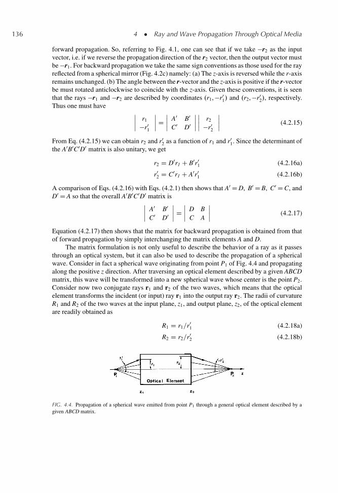
136 4 � Ray and Wave Propagation Through Optical Media
forward propagation. So, referring to Fig. 4.1, one can see that if we take �r2 as the inputvector, i.e. if we reverse the propagation direction of the r2 vector, then the output vector mustbe �r1. For backward propagation we take the same sign conventions as those used for the rayreflected from a spherical mirror (Fig. 4.2c) namely: (a) The z-axis is reversed while the r-axisremains unchanged. (b) The angle between the r-vector and the z-axis is positive if the r-vectorbe must rotated anticlockwise to coincide with the z-axis. Given these conventions, it is seenthat the rays �r1 and �r2 are described by coordinates .r1, �r0
1/ and .r2, �r02/, respectively.
Thus one must have ˇˇ r1
�r01
ˇˇ D
ˇˇ A0 B0
C0 D0
ˇˇˇˇ r2
�r02
ˇˇ (4.2.15)
From Eq. (4.2.15) we can obtain r2 and r02 as a function of r1 and r0
1. Since the determinant ofthe A0B0C0D0 matrix is also unitary, we get
r2 D D0r1 C B0r01 (4.2.16a)
r02 D C0r1 C A0r0
1 (4.2.16b)
A comparison of Eqs. (4.2.16) with Eqs. (4.2.1) then shows that A0 D D, B0 D B, C0 D C, andD0 D A so that the overall A0B0C0D0 matrix isˇ
ˇ A0 B0C0 D0
ˇˇ D
ˇˇ D B
C A
ˇˇ (4.2.17)
Equation (4.2.17) then shows that the matrix for backward propagation is obtained from thatof forward propagation by simply interchanging the matrix elements A and D.
The matrix formulation is not only useful to describe the behavior of a ray as it passesthrough an optical system, but it can also be used to describe the propagation of a sphericalwave. Consider in fact a spherical wave originating from point P1 of Fig. 4.4 and propagatingalong the positive z direction. After traversing an optical element described by a given ABCDmatrix, this wave will be transformed into a new spherical wave whose center is the point P2.Consider now two conjugate rays r1 and r2 of the two waves, which means that the opticalelement transforms the incident (or input) ray r1 into the output ray r2. The radii of curvatureR1 and R2 of the two waves at the input plane, z1, and output plane, z2, of the optical elementare readily obtained as
R1 D r1=r01 (4.2.18a)
R2 D r2=r02 (4.2.18b)
FIG. 4.4. Propagation of a spherical wave emitted from point P1 through a general optical element described by agiven ABCD matrix.
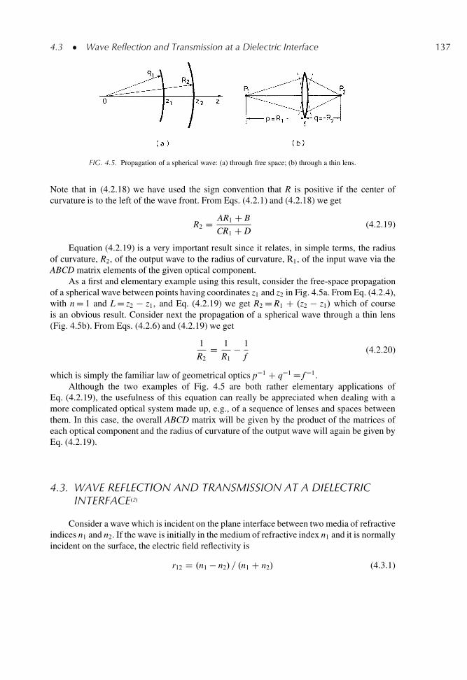
4.3 � Wave Reflection and Transmission at a Dielectric Interface 137
FIG. 4.5. Propagation of a spherical wave: (a) through free space; (b) through a thin lens.
Note that in (4.2.18) we have used the sign convention that R is positive if the center ofcurvature is to the left of the wave front. From Eqs. (4.2.1) and (4.2.18) we get
R2 D AR1 C B
CR1 C D(4.2.19)
Equation (4.2.19) is a very important result since it relates, in simple terms, the radiusof curvature, R2, of the output wave to the radius of curvature, R1, of the input wave via theABCD matrix elements of the given optical component.
As a first and elementary example using this result, consider the free-space propagationof a spherical wave between points having coordinates z1 and z2 in Fig. 4.5a. From Eq. (4.2.4),with n D 1 and L D z2 � z1, and Eq. (4.2.19) we get R2 D R1 C .z2 � z1/ which of courseis an obvious result. Consider next the propagation of a spherical wave through a thin lens(Fig. 4.5b). From Eqs. (4.2.6) and (4.2.19) we get
1
R2D 1
R1� 1
f(4.2.20)
which is simply the familiar law of geometrical optics p�1 C q�1 D f �1.Although the two examples of Fig. 4.5 are both rather elementary applications of
Eq. (4.2.19), the usefulness of this equation can really be appreciated when dealing with amore complicated optical system made up, e.g., of a sequence of lenses and spaces betweenthem. In this case, the overall ABCD matrix will be given by the product of the matrices ofeach optical component and the radius of curvature of the output wave will again be given byEq. (4.2.19).
4.3. WAVE REFLECTION AND TRANSMISSION AT A DIELECTRICINTERFACE.2/
Consider a wave which is incident on the plane interface between two media of refractiveindices n1 and n2. If the wave is initially in the medium of refractive index n1 and it is normallyincident on the surface, the electric field reflectivity is
r12 D .n1 � n2/ = .n1 C n2/ (4.3.1)
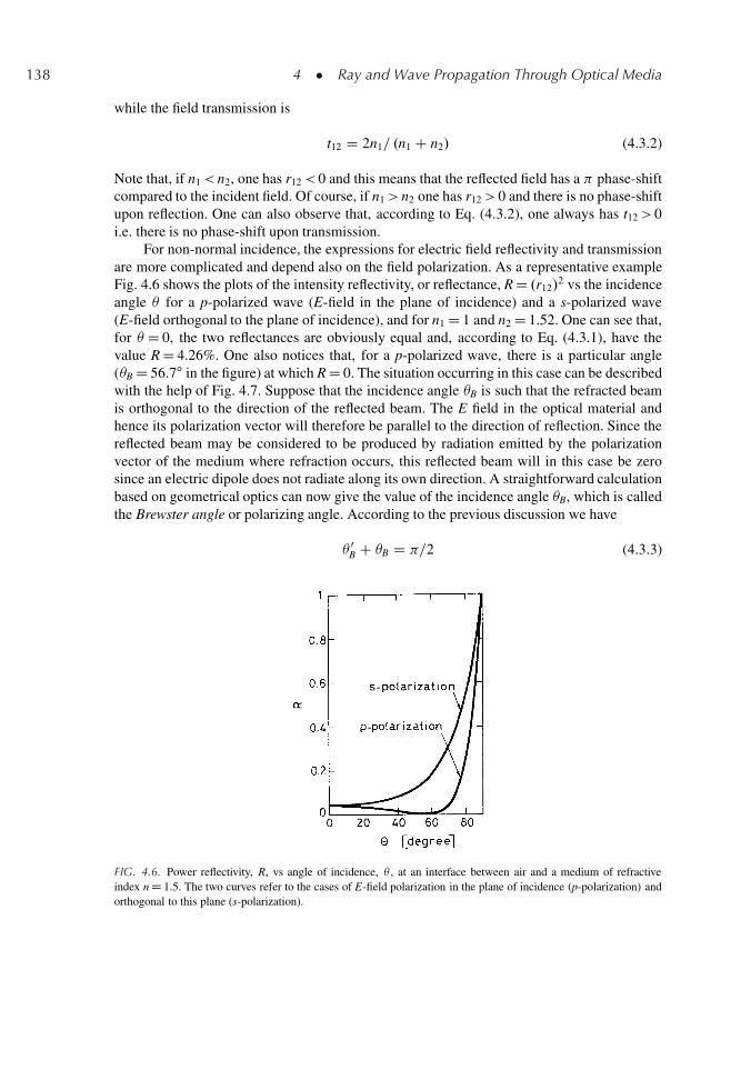
138 4 � Ray and Wave Propagation Through Optical Media
while the field transmission is
t12 D 2n1= .n1 C n2/ (4.3.2)
Note that, if n1< n2, one has r12 < 0 and this means that the reflected field has a phase-shiftcompared to the incident field. Of course, if n1> n2 one has r12> 0 and there is no phase-shiftupon reflection. One can also observe that, according to Eq. (4.3.2), one always has t12> 0i.e. there is no phase-shift upon transmission.
For non-normal incidence, the expressions for electric field reflectivity and transmissionare more complicated and depend also on the field polarization. As a representative exampleFig. 4.6 shows the plots of the intensity reflectivity, or reflectance, R D .r12/
2 vs the incidenceangle for a p-polarized wave (E-field in the plane of incidence) and a s-polarized wave(E-field orthogonal to the plane of incidence), and for n1 D 1 and n2 D 1.52. One can see that,for D 0, the two reflectances are obviously equal and, according to Eq. (4.3.1), have thevalue R D 4.26%. One also notices that, for a p-polarized wave, there is a particular angle(B D 56.7ı in the figure) at which R D 0. The situation occurring in this case can be describedwith the help of Fig. 4.7. Suppose that the incidence angle B is such that the refracted beamis orthogonal to the direction of the reflected beam. The E field in the optical material andhence its polarization vector will therefore be parallel to the direction of reflection. Since thereflected beam may be considered to be produced by radiation emitted by the polarizationvector of the medium where refraction occurs, this reflected beam will in this case be zerosince an electric dipole does not radiate along its own direction. A straightforward calculationbased on geometrical optics can now give the value of the incidence angle B, which is calledthe Brewster angle or polarizing angle. According to the previous discussion we have
0B C B D =2 (4.3.3)
FIG. 4.6. Power reflectivity, R, vs angle of incidence, , at an interface between air and a medium of refractiveindex n D 1.5. The two curves refer to the cases of E-field polarization in the plane of incidence (p-polarization) andorthogonal to this plane (s-polarization).
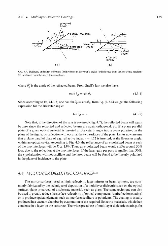
4.4 � Multilayer Dielectric Coatings 139
FIG. 4.7. Reflected and refracted beams for incidence at Brewster’s angle: (a) incidence from the less dense medium;(b) incidence from the more dense medium.
where 0B is the angle of the refracted beam. From Snell’s law we also have
n sin 0B D sin B (4.3.4)
Since according to Eq. (4.3.3) one has sin 0B D cos B, from Eq. (4.3.4) we get the following
expression for the Brewster angle:
tan B D n (4.3.5)
Note that, if the direction of the rays is reversed (Fig. 4.7), the reflected beam will againbe zero since the refracted and reflected beams are again orthogonal. So, if a plane parallelplate of a given optical material is inserted at Brewster’s angle into a beam polarized in theplane of the figure, no reflection will occur at the two surfaces of the plate. Let us now assumethat a plane parallel plate of e.g. refractive index n D 1.52 is inserted, at the Brewster angle,within an optical cavity. According to Fig. 4.6, the reflectance of an s-polarized beam at eachof the two interfaces will be R Š 15%. Thus, an s-polarized beam would suffer around 30%loss, due to the reflection at the two interfaces. If the laser gain per pass is smaller than 30%,the s-polarization will not oscillate and the laser beam will be found to be linearly polarizedin the plane of incidence to the plate.
4.4. MULTILAYER DIELECTRIC COATINGS.3,4/
The mirror surfaces, used as high-reflectivity laser mirrors or beam splitters, are com-monly fabricated by the technique of deposition of a multilayer dielectric stack on the opticalsurface, plane or curved, of a substrate material, such as glass. The same technique can alsobe used to greatly reduce the surface reflectivity of optical components (antireflection coating)or to produce optical elements such as interference filters or polarizers. The coating is usuallyproduced in a vacuum chamber by evaporation of the required dielectric materials, which thencondense in a layer on the substrate. The widespread use of multilayer dielectric coatings for
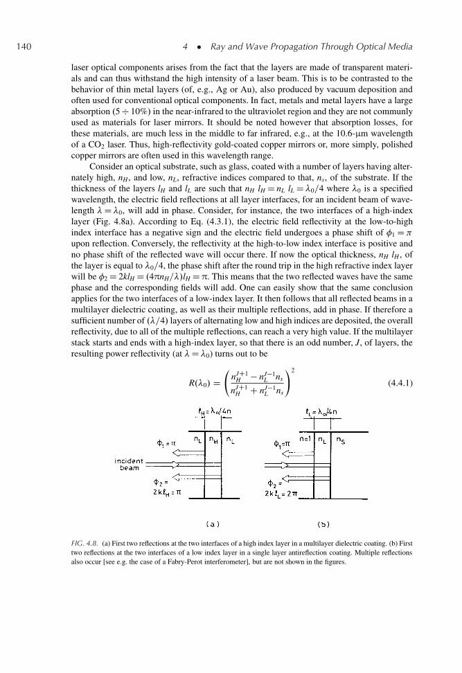
140 4 � Ray and Wave Propagation Through Optical Media
laser optical components arises from the fact that the layers are made of transparent materi-als and can thus withstand the high intensity of a laser beam. This is to be contrasted to thebehavior of thin metal layers (of, e.g., Ag or Au), also produced by vacuum deposition andoften used for conventional optical components. In fact, metals and metal layers have a largeabsorption .5 � 10%/ in the near-infrared to the ultraviolet region and they are not communlyused as materials for laser mirrors. It should be noted however that absorption losses, forthese materials, are much less in the middle to far infrared, e.g., at the 10.6-μm wavelengthof a CO2 laser. Thus, high-reflectivity gold-coated copper mirrors or, more simply, polishedcopper mirrors are often used in this wavelength range.
Consider an optical substrate, such as glass, coated with a number of layers having alter-nately high, nH, and low, nL, refractive indices compared to that, ns, of the substrate. If thethickness of the layers lH and lL are such that nH lH D nL lL D�0=4 where �0 is a specifiedwavelength, the electric field reflections at all layer interfaces, for an incident beam of wave-length �D�0, will add in phase. Consider, for instance, the two interfaces of a high-indexlayer (Fig. 4.8a). According to Eq. (4.3.1), the electric field reflectivity at the low-to-highindex interface has a negative sign and the electric field undergoes a phase shift of �1 D
upon reflection. Conversely, the reflectivity at the high-to-low index interface is positive andno phase shift of the reflected wave will occur there. If now the optical thickness, nH lH , ofthe layer is equal to �0=4, the phase shift after the round trip in the high refractive index layerwill be �2 D 2klH D .4πnH=�/lH D π. This means that the two reflected waves have the samephase and the corresponding fields will add. One can easily show that the same conclusionapplies for the two interfaces of a low-index layer. It then follows that all reflected beams in amultilayer dielectric coating, as well as their multiple reflections, add in phase. If therefore asufficient number of .�=4/ layers of alternating low and high indices are deposited, the overallreflectivity, due to all of the multiple reflections, can reach a very high value. If the multilayerstack starts and ends with a high-index layer, so that there is an odd number, J, of layers, theresulting power reflectivity (at �D�0) turns out to be
R.�0/ D
nJC1H � nJ�1
L ns
nJC1H C nJ�1
L ns
!2
(4.4.1)
FIG. 4.8. (a) First two reflections at the two interfaces of a high index layer in a multilayer dielectric coating. (b) Firsttwo reflections at the two interfaces of a low index layer in a single layer antireflection coating. Multiple reflectionsalso occur [see e.g. the case of a Fabry-Perot interferometer], but are not shown in the figures.
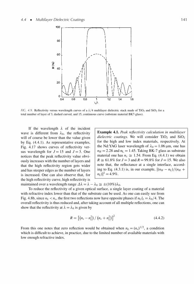
4.4 � Multilayer Dielectric Coatings 141
FIG. 4.9. Reflectivity versus wavelength curves of a �=4 multilayer dielectric stack made of TiO2 and SiO2 for atotal number of layer of 3, dashed curved, and 15, continuous curve (substrate material BK7-glass).
Example 4.1. Peak reflectivity calculation in multilayerdielectric coatings. We will consider TiO2 and SiO2
for the high and low index materials, respectively. Atthe Nd:YAG laser wavelength of �0 D 1.06 μm, one hasnH D 2.28 and nL D 1.45. Taking BK-7 glass as substratematerial one has ns Š 1.54. From Eq. (4.4.1) we obtainR Š 61.8% for J D 3 and R D 99.8% for J D 15. We alsonote that, the reflectance at a single interface, accord-ing to Eq. (4.3.1) is, in our example, Œ.nH � nL/=.nH CnL/�
2 D 4.9%.
If the wavelength � of the incidentwave is different from �0, the reflectivitywill of course be lower than the value givenby Eq. (4.4.1). As representative examples,Fig. 4.17 shows curves of reflectivity ver-sus wavelength for J D 15 and J D 3. Onenotices that the peak reflectivity value obvi-ously increases with the number of layers andthat the high reflectivity region gets widerand has steeper edges as the number of layersis increased. One can also observe that, forthe high reflectivity curve, high reflectivity ismaintained over a wavelength range�D� � �0 Š ˙.10%/�0.
To reduce the reflectivity of a given optical surface, a single layer coating of a materialwith refractive index lower than that of the substrate can be used. As one can easily see fromFig. 4.8b, since nL< ns, the first two reflections now have opposite phases if nLlL D�0=4. Theoverall reflectivity is thus reduced and, after taking account of all multiple reflections, one canshow that the reflectivity at �D�0 is given by
R D �ns � n2
L
�=ns C n2
L
�2(4.4.2)
From this one notes that zero reflection would be obtained when nL D .ns/1=2, a condition
which is difficult to achieve, in practice, due to the limited number of available materials withlow enough refractive index.
142 4 � Ray and Wave Propagation Through Optical Media
Example 4.2. Single layer antireflection coating of laser materials. Consider a BK-7 glass substrate forwhich, at �D 1.06 μm one has ns D 1.54. To achieve zero reflectivity with a single layer, the refractiveindex of the layer material should be nL D Œns�
1=2 Š 1.24. The lowest refractive index material availableas a stable film is provided by MgF2 (Fluorite) with nL D 1.38. From Eq. (4.4.2) we get R Š 1.1% which,although not zero, is still significantly smaller than the reflectivity of the bare surface, which, accordingto Eq. (4.3.1), is given by R D Œ.ns � 1/=.ns C 1/�2 D 4.5%. Fluorite is a rather soft material, however, andit can easily be scratched. Consider next a Nd:YAG rod .ns D 1.82/ and consider a �=4 layer of SiO2, arather hard and durable material .nL D 1.45/, for antireflection coating. From Eq. (4.4.2) we get in thiscase R D 3.4% which while far from perfect is significantly less than the reflectivity of the bare surface.R Š 8.5%/. One notes that Fluorite would provide an almost perfect match, in this case, the reflectivityaccording to Eq. (4.4.2) being reduced to R Š 4 � 10�4.
The minimum reflectivity value given by Eq. (4.4.2) applies, of course, for �D�0. Thewidth of the low reflectivity region, for a single layer coating, is however very large. For exam-ple, if �0 corresponds to the center of the visible range, the reflectivity is reduced below thatof the bare surface for the whole visible range. Quite often, for laser applications, even lowerreflectivities than those considered in example 4.2 may be required (down to perhaps 0.1%).This can be achieved using more than one layer in the antireflection coating. A coating consist-ing of two, �=4, layers of low and high refractive index material, with the sequence ns=nL=nH,is often used for glass. A very hard and durable two-layer coating, which is often used isZrO2 .nH D 2.1/-MgF2 .nL D 1.38/. The region of low reflectivity is reduced, for this type ofcoating, with the reflectivity versus wavelength curve having a sharp, V-shaped, minimum.Such a coating is commonly referred to as a V-coating.
4.5. THE FABRY-PEROT INTERFEROMETER.5/
We now go on to consider a second example of multiple interference, the case of aFabry-Perot (FP) interferometer. This interferometer, a common spectroscopic tool since itsintroduction in 1899, plays a very important role in laser physics for at least three differentreasons: (1) On a fundamental level its physical behavior forms a basis to the behavior ofoptical resonators. (2) It is often used as a frequency selective element in a laser cavity. (3) Itis often used as a spectrometer for analyzing the spectrum of the light emitted by a laser.
4.5.1. Properties of a Fabry-Perot Interferometer
The FP interferometer consists of two plane or spherical mirrors with power reflectivitiesR1 and R2, separated by a distance L and containing a medium of refractive index nr. Although,for the ultimate performance, interferometers make use of spherical mirrors, we will, forsimplicity, consider here the case of two plane and parallel mirrors. In this case, consider aplane wave of frequency � incident on the interferometer in a direction making an angle 0with the normal to the two mirrors (Fig. 4.10). This wave is indicated schematically by the ray
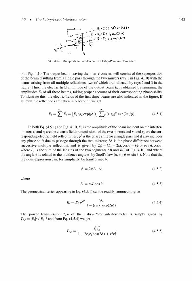
4.5 � The Fabry-Perot Interferometer 143
FIG. 4.10. Multiple-beam interference in a Fabry-Perot interferometer.
0 in Fig. 4.10. The output beam, leaving the interferometer, will consist of the superpositionof the beam resulting from a single pass through the two mirrors (ray 1 in Fig. 4.10) with thebeams arising from all multiple reflections, two of which are indicated by rays 2 and 3 in thefigure. Thus, the electric field amplitude of the output beam Et is obtained by summing theamplitudes El of all these beams, taking proper account of their corresponding phase-shifts.To illustrate this, the electric fields of the first three beams are also indicated in the figure. Ifall multiple reflections are taken into account, we get
Et D1X1
lEl D �E0t1t2 exp.j�0/
1X0
m.r1r2/m exp.2mj�/ (4.5.1)
In both Eq. (4.5.1) and Fig. 4.10, E0 is the amplitude of the beam incident on the interfer-ometer; t1 and t2 are the electric field transmissions of the two mirrors and r1 and r2 are the cor-responding electric field reflectivities; �0 is the phase shift for a single pass and it also includesany phase shift due to passage through the two mirrors; 2� is the phase difference betweensuccessive multiple reflections and is given by 2�D kLs D 2kL cos D .4πnr�=c/L cos ,where Ls is the sum of the lengths of the two segments AB and BC of Fig. 4.10, and wherethe angle is related to the incidence angle 0 by Snell’s law .nr sin D sin 0/. Note that theprevious expression can, for simplicity, be transformed to
� D 2 L0�=c (4.5.2)
whereL0 D nrL cos (4.5.3)
The geometrical series appearing in Eq. (4.5.1) can be readily summed to give
Et D E0 ej0 t1t21 � .r1r2/ exp.2j�/
(4.5.4)
The power transmission TFP of the Fabry-Perot interferometer is simply given byTFP D jEtj2=jE0j2 and from Eq. (4.5.4) we get
TFP D t21 t2
2
1 � 2r1r2 cos.2�/C r21r2
2
(4.5.5)
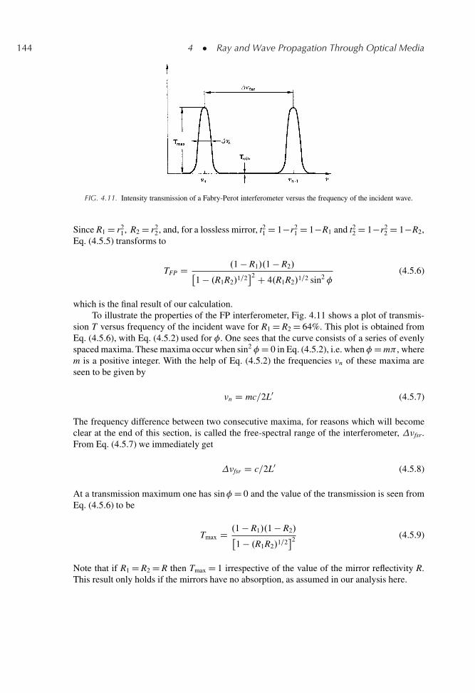
144 4 � Ray and Wave Propagation Through Optical Media
FIG. 4.11. Intensity transmission of a Fabry-Perot interferometer versus the frequency of the incident wave.
Since R1 D r21, R2 D r2
2, and, for a lossless mirror, t21 D 1�r2
1 D 1�R1 and t22 D 1�r2
2 D 1�R2,Eq. (4.5.5) transforms to
TFP D .1 � R1/.1 � R2/�1 � .R1R2/1=2
2 C 4.R1R2/1=2 sin2 �(4.5.6)
which is the final result of our calculation.To illustrate the properties of the FP interferometer, Fig. 4.11 shows a plot of transmis-
sion T versus frequency of the incident wave for R1 D R2 D 64%. This plot is obtained fromEq. (4.5.6), with Eq. (4.5.2) used for �. One sees that the curve consists of a series of evenlyspaced maxima. These maxima occur when sin2 �D 0 in Eq. (4.5.2), i.e. when �D m , wherem is a positive integer. With the help of Eq. (4.5.2) the frequencies �n of these maxima areseen to be given by
�n D mc=2L0 (4.5.7)
The frequency difference between two consecutive maxima, for reasons which will becomeclear at the end of this section, is called the free-spectral range of the interferometer, �fsr.From Eq. (4.5.7) we immediately get
�fsr D c=2L0 (4.5.8)
At a transmission maximum one has sin�D 0 and the value of the transmission is seen fromEq. (4.5.6) to be
Tmax D .1 � R1/.1 � R2/�1 � .R1R2/1=2
2 (4.5.9)
Note that if R1 D R2 D R then Tmax D 1 irrespective of the value of the mirror reflectivity R.This result only holds if the mirrors have no absorption, as assumed in our analysis here.
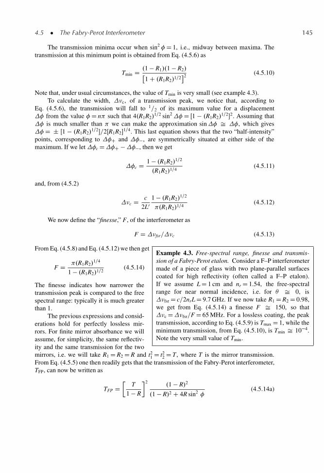
4.5 � The Fabry-Perot Interferometer 145
The transmission minima occur when sin2 �D 1, i.e., midway between maxima. Thetransmission at this minimum point is obtained from Eq. (4.5.6) as
Tmin D .1 � R1/.1 � R2/�1 C .R1R2/1=2
2 (4.5.10)
Note that, under usual circumstances, the value of Tmin is very small (see example 4.3).To calculate the width, �c, of a transmission peak, we notice that, according to
Eq. (4.5.6), the transmission will fall to 1=2 of its maximum value for a displacement� from the value �D n such that 4.R1R2/
1=2 sin2�D Œ1 � .R1R2/1=2�2. Assuming that
� is much smaller than we can make the approximation sin� Š �, which gives�D ˙ Œ1 � .R1R2/
1=2�=2ŒR1R2�1=4. This last equation shows that the two “half-intensity”
points, corresponding to �C and ��, are symmetrically situated at either side of themaximum. If we let �c D�C ���, then we get
�c D 1 � .R1R2/1=2
.R1R2/1=4(4.5.11)
and, from (4.5.2)
�c D c
2L01 � .R1R2/
1=2
.R1R2/1=4(4.5.12)
We now define the “finesse,” F, of the interferometer as
F D �fsr=�c (4.5.13)
Example 4.3. Free-spectral range, finesse and transmis-sion of a Fabry-Perot etalon. Consider a F–P interferometermade of a piece of glass with two plane-parallel surfacescoated for high reflectivity (often called a F–P etalon).If we assume L D 1 cm and nr D 1.54, the free-spectralrange for near normal incidence, i.e. for Š 0, is�fsr D c=2nrL D 9.7 GHz. If we now take R1 D R2 D 0.98,we get from Eq. (4.5.14) a finesse F Š 150, so that�c D�fsr=F D 65 MHz. For a lossless coating, the peaktransmission, according to Eq. (4.5.9) is Tmax D 1, while theminimum transmission, from Eq. (4.5.10), is Tmin Š 10�4.Note the very small value of Tmin.
From Eq. (4.5.8) and Eq. (4.5.12) we then get
F D .R1R2/1=4
1 � .R1R2/1=2(4.5.14)
The finesse indicates how narrower thetransmission peak is compared to the freespectral range: typically it is much greaterthan 1.
The previous expressions and consid-erations hold for perfectly lossless mir-rors. For finite mirror absorbance we willassume, for simplicity, the same reflectiv-ity and the same transmission for the twomirrors, i.e. we will take R1 D R2 D R and t2
1 D t22 D T, where T is the mirror transmission.
From Eq. (4.5.5) one then readily gets that the transmission of the Fabry-Perot interferometer,TFP, can now be written as
TFP D�
T
1 � R
�2.1 � R/2
.1 � R/2 C 4R sin2 �(4.5.14a)
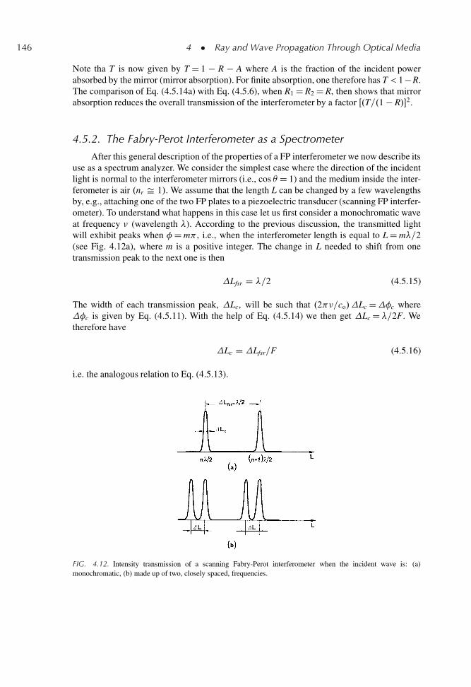
146 4 � Ray and Wave Propagation Through Optical Media
Note tha T is now given by T D 1 � R � A where A is the fraction of the incident powerabsorbed by the mirror (mirror absorption). For finite absorption, one therefore has T < 1 � R.The comparison of Eq. (4.5.14a) with Eq. (4.5.6), when R1 D R2 D R, then shows that mirrorabsorption reduces the overall transmission of the interferometer by a factor Œ.T=.1 � R/�2.
4.5.2. The Fabry-Perot Interferometer as a Spectrometer
After this general description of the properties of a FP interferometer we now describe itsuse as a spectrum analyzer. We consider the simplest case where the direction of the incidentlight is normal to the interferometer mirrors (i.e., cos D 1) and the medium inside the inter-ferometer is air .nr Š 1/. We assume that the length L can be changed by a few wavelengthsby, e.g., attaching one of the two FP plates to a piezoelectric transducer (scanning FP interfer-ometer). To understand what happens in this case let us first consider a monochromatic waveat frequency � (wavelength �). According to the previous discussion, the transmitted lightwill exhibit peaks when �D m , i.e., when the interferometer length is equal to L D m�=2(see Fig. 4.12a), where m is a positive integer. The change in L needed to shift from onetransmission peak to the next one is then
Lfsr D �=2 (4.5.15)
The width of each transmission peak, Lc, will be such that .2 �=co/Lc D�c where�c is given by Eq. (4.5.11). With the help of Eq. (4.5.14) we then get Lc D�=2F. Wetherefore have
Lc D Lfsr=F (4.5.16)
i.e. the analogous relation to Eq. (4.5.13).
FIG. 4.12. Intensity transmission of a scanning Fabry-Perot interferometer when the incident wave is: (a)monochromatic, (b) made up of two, closely spaced, frequencies.
4.6 � Diffraction Optics in the Paraxial Approximation 147
We now consider the case where two waves at frequencies � and � C � are incidenton the interferometer. The wave at frequency .� C �/ will produce a set of transmissionpeaks displaced by a quantityL from those corresponding to frequency � (Fig. 4.12b). Since2 Lv=c D nπ, the displacement L must be such that 2 .L C L/.� C �/=c D n , i.e.such that L D � .�=�/L. The two frequencies � and � C � will be resolved by thespectrometer if jLj Lc. The equality sign in this expression corresponds to the minimumfrequency interval �m which can be resolved, which gives .�m=�/L DLc. With the helpof Eq. (4.5.16) and Eq. (4.5.15) we then get .�m=�/L D�=2F. Using Eq. (4.5.8) with L0 D Lwe obtain
�m D �fsr=F (4.5.17)
Example 4.4. Spectral measurement of an ArC-laseroutput beam. We will consider an Ar-ion laser oscillat-ing on its green line at �D 514.5 nm wavelength. Wewill assume the laser to be oscillating on many lon-gitudinal modes encompassing the full Doppler widthof the laser line .��
0 D 3.5 GHz/. We will thus have�osc D��
0 D 3.5 GHz. To avoid frequency ambiguity,we must have �fsr D .c=2L/ 3.5 GHz i.e. L 4.28 cm. If we now assume a finesse F D 150 andtake L D 4.28 cm, according to Eq. (4.5.18) we have,for the interferometer resolution, �m D�osc=F Š23 MHz. If, for example, the length of the laser cavityis L1 D 1.5 m, consecutive longitudinal modes are sep-arated (see next Chapter) by �D c=2L1 D 100 MHz.Thus, since �m<�, the FP interferometer is able toresolve these longitudinal modes. One can also observethat, since the frequency of the laser light is �D c=� Š5.83 � 1014 Hz, the corresponding resolving power of theinterferometer is �=�m D 2.54 �107. This is a very highresolving power compared, e.g., to the best that can beobtained with a grating spectrometer .�=� < 106/.
Thus the finesse of the interferometerspecifies its resolving power in terms of thefree spectral range.
It must be noted that when jLj DLfsr,i.e. when �D�fsr D c=2L, the transmis-sion peaks at frequencies � C � and �
will be coincident, although shifted by oneorder relative to each other. Therefore, when� >�fsr, an ambiguity by a multiple of�fsr occurs in the measurement of �.Thus, when using the interferometer to pro-vide a measurement of frequency difference,a simple and unambiguous result is onlyobtained when � <�fsr, which explainswhy �fsr is called the free spectral range ofthe interferometer. We can readily generalizethe above result and say that if �osc is thespectral bandwidth of the incident light, thento avoid frequency ambiguity, we must have�osc �fsr. If the equality is assumed tohold in this relation, then from Eq. (4.5.17)we get
�m D �osc=F (4.5.18)
Thus the finesse F also provides a measure of how finely we can discriminate frequencieswithin the total spectral bandwidth�osc.
4.6. DIFFRACTION OPTICS IN THE PARAXIAL APPROXIMATION.6/
We shall consider a monochromatic wave under the so-called scalar approximation wherethe e.m. fields are uniformly (e.g. linearly or circularly) polarized. The electric field of thewave can then be described by a scalar quantity viz
E.x, y, z, t/ D QE.x, y, z/ exp.j!t/ (4.6.1)
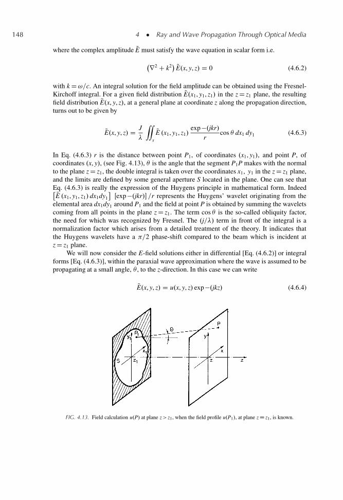
148 4 � Ray and Wave Propagation Through Optical Media
where the complex amplitude QE must satisfy the wave equation in scalar form i.e.
r2 C k2� QE.x, y, z/ D 0 (4.6.2)
with k D!=c. An integral solution for the field amplitude can be obtained using the Fresnel-Kirchoff integral. For a given field distribution QE.x1, y1, z1/ in the z D z1 plane, the resultingfield distribution QE.x, y, z/, at a general plane at coordinate z along the propagation direction,turns out to be given by
QE.x, y, z/ D J
�
“s
QE .x1, y1, z1/exp �.jkr/
rcos dx1 dy1 (4.6.3)
In Eq. (4.6.3) r is the distance between point P1, of coordinates .x1, y1/, and point P, ofcoordinates .x, y/, (see Fig. 4.13), is the angle that the segment P1P makes with the normalto the plane z D z1, the double integral is taken over the coordinates x1, y1 in the z D z1 plane,and the limits are defined by some general aperture S located in the plane. One can see thatEq. (4.6.3) is really the expression of the Huygens principle in mathematical form. Indeed� QE .x1, y1, z1/ dx1dy1
Œexp �.jkr/� =r represents the Huygens’ wavelet originating from the
elemental area dx1dy1 around P1 and the field at point P is obtained by summing the waveletscoming from all points in the plane z D z1. The term cos is the so-called obliquity factor,the need for which was recognized by Fresnel. The .j=�/ term in front of the integral is anormalization factor which arises from a detailed treatment of the theory. It indicates thatthe Huygens wavelets have a =2 phase-shift compared to the beam which is incident atz D z1 plane.
We will now consider the E-field solutions either in differential [Eq. (4.6.2)] or integralforms [Eq. (4.6.3)], within the paraxial wave approximation where the wave is assumed to bepropagating at a small angle, , to the z-direction. In this case we can write
QE.x, y, z/ D u.x, y, z/ exp �.jkz/ (4.6.4)
FIG. 4.13. Field calculation u.P/ at plane z> z1, when the field profile u.P1/, at plane z D z1, is known.
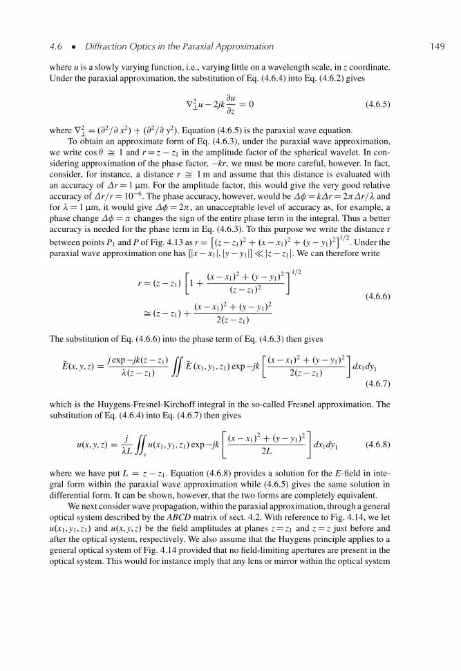
4.6 � Diffraction Optics in the Paraxial Approximation 149
where u is a slowly varying function, i.e., varying little on a wavelength scale, in z coordinate.Under the paraxial approximation, the substitution of Eq. (4.6.4) into Eq. (4.6.2) gives
r2?u � 2jk@u
@zD 0 (4.6.5)
where r2? D .@2=@ x2/C .@2=@ y2/. Equation (4.6.5) is the paraxial wave equation.
To obtain an approximate form of Eq. (4.6.3), under the paraxial wave approximation,we write cos Š 1 and r D z � z1 in the amplitude factor of the spherical wavelet. In con-sidering approximation of the phase factor, �kr, we must be more careful, however. In fact,consider, for instance, a distance r Š 1 m and assume that this distance is evaluated withan accuracy of r D 1 μm. For the amplitude factor, this would give the very good relativeaccuracy ofr=r D 10�6. The phase accuracy, however, would be �D kr D 2 r=� andfor �D 1 μm, it would give �D 2 , an unacceptable level of accuracy as, for example, aphase change �D changes the sign of the entire phase term in the integral. Thus a betteraccuracy is needed for the phase term in Eq. (4.6.3). To this purpose we write the distance r
between points P1 and P of Fig. 4.13 as r D �.z � z1/
2 C .x � x1/2 C .y � y1/
21=2
. Under theparaxial wave approximation one has Œjx � x1j, jy � y1j�� jz � z1j. We can therefore write
r D .z � z1/
�1 C .x � x1/
2 C .y � y1/2
.z � z1/2
� 1=2
Š .z � z1/C .x � x1/2 C .y � y1/
2
2.z � z1/
(4.6.6)
The substitution of Eq. (4.6.6) into the phase term of Eq. (4.6.3) then gives
QE.x, y, z/ D j exp �jk.z � z1/
�.z � z1/
“QE .x1, y1, z1/ exp �jk
�.x � x1/
2 C .y � y1/2
2.z � z1/
�dx1dy1
(4.6.7)
which is the Huygens-Fresnel-Kirchoff integral in the so-called Fresnel approximation. Thesubstitution of Eq. (4.6.4) into Eq. (4.6.7) then gives
u.x, y, z/ D j
�L
“s
u.x1, y1, z1/ exp �jk
".x � x1/
2 C .y � y1/2
2L
#dx1dy1 (4.6.8)
where we have put L D z � z1. Equation (4.6.8) provides a solution for the E-field in inte-gral form within the paraxial wave approximation while (4.6.5) gives the same solution indifferential form. It can be shown, however, that the two forms are completely equivalent.
We next consider wave propagation, within the paraxial approximation, through a generaloptical system described by the ABCD matrix of sect. 4.2. With reference to Fig. 4.14, we letu.x1, y1, z1/ and u.x, y, z/ be the field amplitudes at planes z D z1 and z D z just before andafter the optical system, respectively. We also assume that the Huygens principle applies to ageneral optical system of Fig. 4.14 provided that no field-limiting apertures are present in theoptical system. This would for instance imply that any lens or mirror within the optical system
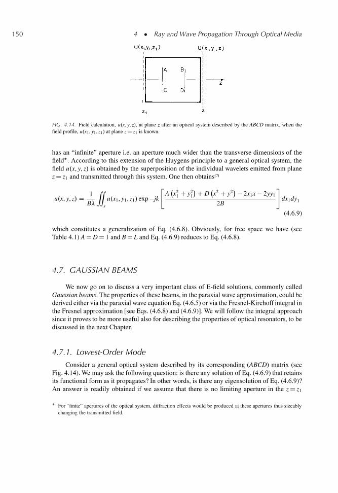
150 4 � Ray and Wave Propagation Through Optical Media
FIG. 4.14. Field calculation, u.x, y, z/, at plane z after an optical system described by the ABCD matrix, when thefield profile, u.x1, y1, z1/ at plane z D z1 is known.
has an “infinite” aperture i.e. an aperture much wider than the transverse dimensions of thefield�. According to this extension of the Huygens principle to a general optical system, thefield u.x, y, z/ is obtained by the superposition of the individual wavelets emitted from planez D z1 and transmitted through this system. One then obtains.7/
u.x, y, z/ D 1
B�
“s
u.x1, y1, z1/ exp �jk
"Ax2
1 C y21
�C Dx2 C y2
�� 2x1x � 2yy1
2B
#dx1dy1
(4.6.9)
which constitutes a generalization of Eq. (4.6.8). Obviously, for free space we have (seeTable 4.1) A D D D 1 and B D L and Eq. (4.6.9) reduces to Eq. (4.6.8).
4.7. GAUSSIAN BEAMS
We now go on to discuss a very important class of E-field solutions, commonly calledGaussian beams. The properties of these beams, in the paraxial wave approximation, could bederived either via the paraxial wave equation Eq. (4.6.5) or via the Fresnel-Kirchoff integral inthe Fresnel approximation [see Eqs. (4.6.8) and (4.6.9)]. We will follow the integral approachsince it proves to be more useful also for describing the properties of optical resonators, to bediscussed in the next Chapter.
4.7.1. Lowest-Order Mode
Consider a general optical system described by its corresponding (ABCD) matrix (seeFig. 4.14). We may ask the following question: is there any solution of Eq. (4.6.9) that retainsits functional form as it propagates? In other words, is there any eigensolution of Eq. (4.6.9)?An answer is readily obtained if we assume that there is no limiting aperture in the z D z1
� For “finite” apertures of the optical system, diffraction effects would be produced at these apertures thus sizeablychanging the transmitted field.
4.7 � Gaussian Beams 151
plane so that the double integral of Eq. (4.6.9) can be taken between �1 and C1 for bothx1 and y1 variables. In this case we can readily show by direct substitution in Eq. (4.6.9) that
u.x, y, z/ / exp �jk�
x2 C y2�=2q
(4.7.1)
where q D q.z/ is a complex parameter (often called the complex beam parameter of aGaussian beam), is an eigensolution of Eq. (4.6.9). If we write, in fact,
u .x1, y1, z1/ / exp �jk�
x21 C y2
1
�=2q1
(4.7.2)
we get from Eq. (4.6.9)
u.x, y, z/ D 1
A C .B=q1/exp �jk
x2 C y2
2q(4.7.3)
where q is related to q1 by the very simple law
q D A q1 C B
C q1 C D(4.7.4)
Equation (4.7.4) is a very important relation, known as the ABCD law of Gaussian beampropagation. It bears an obvious similarity to Eq. (4.2.19) which shows how the radius ofcurvature of a spherical wave is transformed by an optical system. We will come back to thisequation in sect. 4.7.3. for a deeper discussion.
We now go on to discuss a physical interpretation of the Gaussian solution of Eq. (4.7.1).For this we use Eqs. (4.7.1) and (4.6.4) and write
QE / exp �jk
�z C x2 C y2
2q
�(4.7.5)
Consider now a spherical wave with center at coordinates x D y D z D 0. Its field at pointP.x, y, z/ can be written as QE / Œexp �jk R� =R, where R is the wave’s radius of curva-ture. Within the paraxial approximation, following a similar argument to that in Eq. (4.6.6),we write
R Š z C x2 C y2
2 R(4.7.6)
and the field of the spherical wave transforms to
QE / exp �jk
�z C x2 C y2
2 R
�(4.7.7)
A comparison of Eq. (4.7.7) with Eq. (4.7.5) then shows that the Gaussian beam can be lookedupon as a spherical wave of complex radius of curvature, q. To understand the meaning of thiscomplex beam parameter we separate the real and imaginary part of 1=q, i.e. we write
1
qD 1
R� j
�
w2(4.7.8)
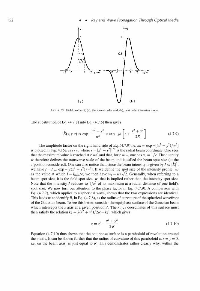
152 4 � Ray and Wave Propagation Through Optical Media
FIG. 4.15. Field profile of, (a), the lowest order and, (b), next order Gaussian mode.
The substitution of Eq. (4.7.8) into Eq. (4.7.5) then gives
QE.x, y, z/ / exp �x2 C y2
w2� exp �jk
�z C x2 C y2
2R
�(4.7.9)
The amplitude factor on the right hand side of Eq. (4.7.9) i.e. u0 D exp �Œ.x2 C y2/=w2�
is plotted in Fig. 4.15a vs r=w, where r D Œx2 C y2�1=2 is the radial beam coordinate. One seesthat the maximum value is reached at r D 0 and that, for r D w, one has u0 D 1=e. The quantityw therefore defines the transverse scale of the beam and is called the beam spot size (at thez-position considered). One can also notice that, since the beam intensity is given by I / j QEj2,we have I D Imax exp �Œ2.x2 C y2/=w2�. If we define the spot size of the intensity profile, wI
as the value at which I D Imax=e, we then have wI D w=p
2. Generally, when referring to abeam spot size, it is the field spot size, w, that is implied rather than the intensity spot size.Note that the intensity I reduces to 1=e2 of its maximum at a radial distance of one field’sspot size. We now turn our attention to the phase factor in Eq. (4.7.9). A comparison withEq. (4.7.7), which applies to a spherical wave, shows that the two expressions are identical.This leads us to identify R, in Eq. (4.7.8), as the radius of curvature of the spherical wavefrontof the Gaussian beam. To see this better, consider the equiphase surface of the Gaussian beamwhich intercepts the z axis at a given position z0. The x, y, z coordinates of this surface mustthen satisfy the relation kz C k.x2 C y2/=2R D kz0, which gives
z D z0 � x2 C y2
2 R(4.7.10)
Equation (4.7.10) thus shows that the equiphase surface is a paraboloid of revolution aroundthe z-axis. It can be shown further that the radius of curvature of this paraboloid at x D y D 0,i.e. on the beam axis, is just equal to R. This demonstrates rather clearly why, within the
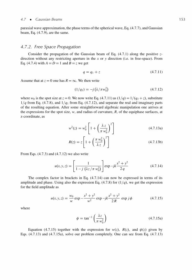
4.7 � Gaussian Beams 153
paraxial wave approximation, the phase terms of the spherical wave, Eq. (4.7.7), and Gaussianbeam, Eq. (4.7.9), are the same.
4.7.2. Free Space Propagation
Consider the propagation of the Gaussian beam of Eq. (4.7.1) along the positive z-direction without any restricting aperture in the x or y direction (i.e. in free-space). FromEq. (4.7.4) with A D D D 1 and B D z we get
q D q1 C z (4.7.11)
Assume that at z D 0 one has R D 1. We then write
.1=q1/ D �j�= w2
0
�(4.7.12)
where w0 is the spot size at z D 0. We now write Eq. (4.7.11) as .1=q/D 1=.q1 C z/, substitute1=q from Eq. (4.7.8), and 1=q1 from Eq. (4.7.12), and separate the real and imaginary partsof the resulting equation. After some straightforward algebraic manipulation one arrives atthe expressions for the spot size, w, and radius of curvature, R, of the equiphase surfaces, atz-coordinate, as
w2.z/ D w20
"1 C
�� z
w20
�2#
(4.7.13a)
R.z/ D z
"1 C
� w2
0
� z
�2#
(4.7.13b)
From Eqs. (4.7.3) and (4.7.12) we also write
u.x, y, z/ D"
1
1 � j�z = w2
0
�#
exp �jkx2 C y2
2 q(4.7.14)
The complex factor in brackets in Eq. (4.7.14) can now be expressed in terms of itsamplitude and phase. Using also the expression Eq. (4.7.8) for .1=q/, we get the expressionfor the field amplitude as
u.x, y, z/ D w0
wexp �x2 C y2
w2exp �jk
x2 C y2
2 Rexp j� (4.7.15)
where
� D tan�1
��z
w20
�(4.7.15a)
Equation (4.7.15) together with the expression for w.z/, R.z/, and �.z/ given byEqs. (4.7.13) and (4.7.15a), solve our problem completely. One can see from Eq. (4.7.13)
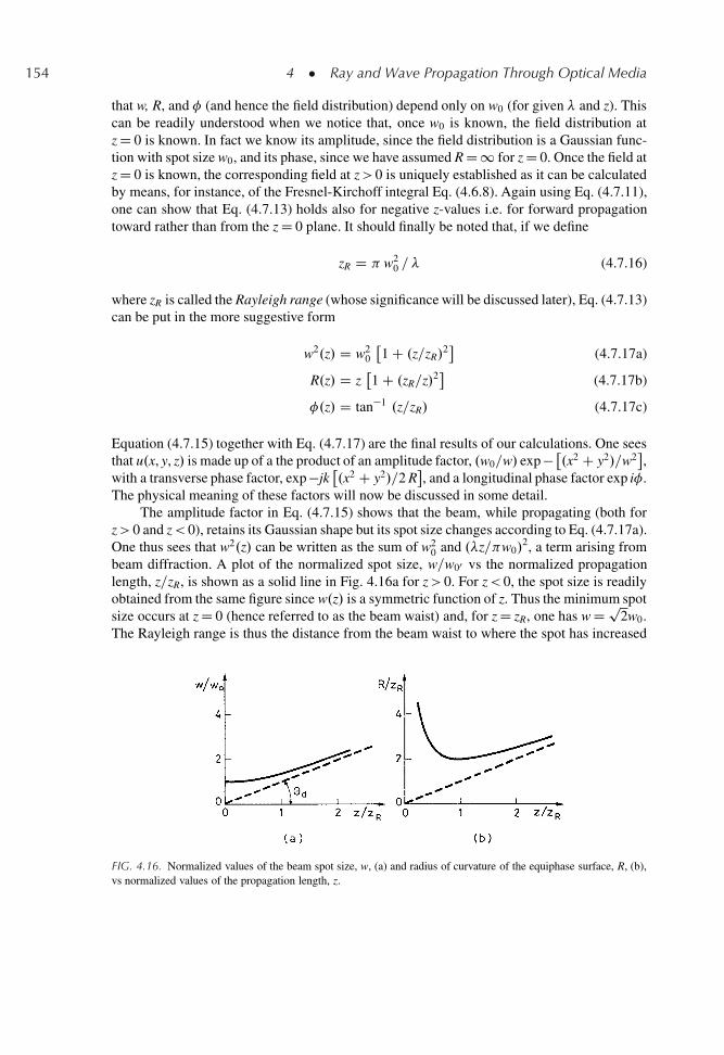
154 4 � Ray and Wave Propagation Through Optical Media
that w, R, and � (and hence the field distribution) depend only on w0 (for given � and z). Thiscan be readily understood when we notice that, once w0 is known, the field distribution atz D 0 is known. In fact we know its amplitude, since the field distribution is a Gaussian func-tion with spot size w0, and its phase, since we have assumed R D 1 for z D 0. Once the field atz D 0 is known, the corresponding field at z> 0 is uniquely established as it can be calculatedby means, for instance, of the Fresnel-Kirchoff integral Eq. (4.6.8). Again using Eq. (4.7.11),one can show that Eq. (4.7.13) holds also for negative z-values i.e. for forward propagationtoward rather than from the z D 0 plane. It should finally be noted that, if we define
zR D w20 = � (4.7.16)
where zR is called the Rayleigh range (whose significance will be discussed later), Eq. (4.7.13)can be put in the more suggestive form
w2.z/ D w20
�1 C .z=zR/
2
(4.7.17a)
R.z/ D z�1 C .zR=z/2
(4.7.17b)
�.z/ D tan�1 .z=zR/ (4.7.17c)
Equation (4.7.15) together with Eq. (4.7.17) are the final results of our calculations. One seesthat u.x, y, z/ is made up of a the product of an amplitude factor, .w0=w/ exp � �.x2 C y2/=w2
,
with a transverse phase factor, exp �jk�.x2 C y2/=2 R
, and a longitudinal phase factor exp i�.
The physical meaning of these factors will now be discussed in some detail.The amplitude factor in Eq. (4.7.15) shows that the beam, while propagating (both for
z> 0 and z< 0), retains its Gaussian shape but its spot size changes according to Eq. (4.7.17a).One thus sees that w2.z/ can be written as the sum of w2
0 and .�z= w0/2, a term arising from
beam diffraction. A plot of the normalized spot size, w=w00 vs the normalized propagationlength, z=zR, is shown as a solid line in Fig. 4.16a for z> 0. For z< 0, the spot size is readilyobtained from the same figure since w.z/ is a symmetric function of z. Thus the minimum spotsize occurs at z D 0 (hence referred to as the beam waist) and, for z D zR, one has w D p
2w0.The Rayleigh range is thus the distance from the beam waist to where the spot has increased
FIG. 4.16. Normalized values of the beam spot size, w, (a) and radius of curvature of the equiphase surface, R, (b),vs normalized values of the propagation length, z.
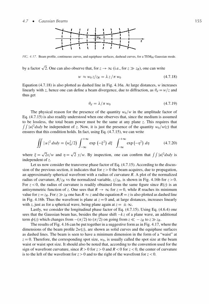
4.7 � Gaussian Beams 155
FIG. 4.17. Beam profile, continuous curves, and equiphase surfaces, dashead curves, for a TEM00 Gaussian mode.
by a factorp
2. One can also observe that, for z ! 1 (i.e., for z � zR), one can write
w � w0 z=zR D � z = w0 (4.7.18)
Equation (4.7.18) is also plotted as dashed line in Fig. 4.16a. At large distances, w increaseslinearly with z, hence one can define a beam divergence, due to diffraction, as d D w=z andthus get
d D �= w0 (4.7.19)
The physical reason for the presence of the quantity w0=w in the amplitude factor ofEq. (4.7.15) is also readily understood when one observes that, since the medium is assumedto be lossless, the total beam power must be the same at any plane z. This requires thatR R juj2dxdy be independent of z. Now, it is just the presence of the quantity w0=w.z/ thatensures that this condition holds. In fact, using Eq. (4.7.15), we can write
“j u j2 dxdy D
w20=2
� Z C1
�1exp
��2�
d�Z C1
�1exp
��2�
d� (4.7.20)
where �D p2x=w and �D p
2 y=w. By inspection, one can confirm thatR R juj2dxdy is
independent of z.Let us now consider the transverse phase factor of Eq. (4.7.15). According to the discus-
sion of the previous section, it indicates that for z> 0 the beam acquires, due to propagation,an approximately spherical wavefront with a radius of curvature R. A plot of the normalizedradius of curvature, R=zR vs the normalized variable, z=zR, is shown in Fig. 4.16b for z> 0.For z< 0, the radius of curvature is readily obtained from the same figure since R.z/ is anantisymmetric function of z. One sees that R ! 1 for z D 0, while R reaches its minimumvalue for z D zR. For z � zR one has R � z and the equation R D z is also plotted as dashed linein Fig. 4.16b. Thus the wavefront is plane at z D 0 and, at large distances, increases linearlywith z, just as for a spherical wave, being plane again at z D ˙ 1.
Lastly, we consider the longitudinal phase factor of Eq. (4.7.15). Using Eq. (4.6.4) onesees that the Gaussian beam has, besides the phase shift �k z of a plane wave, an additionalterm �.z/ which changes from �. =2/ to . =2/ on going from z � � zR to z � zR.
The results of Fig. 4.16 can be put together in a suggestive form as in Fig. 4.17, where thedimensions of the beam profile 2w.z/, are shown as solid curves and the equiphase surfacesas dashed lines. The beam is seen to have a minimum dimension in the form of a “waist” atz D 0. Therefore, the corresponding spot size, w0, is usually called the spot size at the beamwaist or waist spot size. It should also be noted that, according to the convention used for thesign of wavefront curvature, since R> 0 for z> 0 and R< 0 for z< 0, the center of curvatureis to the left of the wavefront for z> 0 and to the right of the wavefront for z< 0.
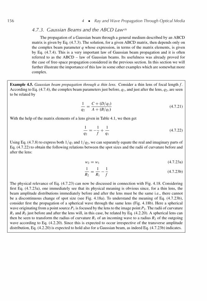
156 4 � Ray and Wave Propagation Through Optical Media
4.7.3. Gaussian Beams and the ABCD Law.8/
The propagation of a Gaussian beam through a general medium described by an ABCDmatrix is given by Eq. (4.7.3). The solution, for a given ABCD matrix, then depends only onthe complex beam parameter q whose expression, in terms of the matrix elements, is givenby Eq. (4.7.4). This is a very important law of Gaussian beam propagation and it is oftenreferred to as the ABCD – law of Gaussian beams. Its usefulness was already proved forthe case of free-space propagation considered in the previous section. In this section we willfurther illustrate the importance of this law in some other examples which are somewhat morecomplex.
Example 4.5. Gaussian beam propagation through a thin lens. Consider a thin lens of focal length f .According to Eq. (4.7.4), the complex beam parameters just before, q1, and just after the lens, q2, are seento be related by
1
q2D C C .D=q1/
A C .B=q1/(4.7.21)
With the help of the matrix elements of a lens given in Table 4.1, we then get
1
q2D �1
fC 1
q1(4.7.22)
Using Eq. (4.7.8) to express both 1=q1 and 1=q2, we can separately equate the real and imaginary parts ofEq. (4.7.22) to obtain the following relations between the spot sizes and the radii of curvature before andafter the lens:
w2 D w1 (4.7.23a)
1
R2D 1
R1� 1
f(4.7.23b)
The physical relevance of Eq. (4.7.23) can now be discussed in connection with Fig. 4.18. Consideringfirst Eq. (4.7.23a), one immediately see that its physical meaning is obvious since, for a thin lens, thebeam amplitude distributions immediately before and after the lens must be the same i.e., there cannotbe a discontinuous change of spot size (see Fig. 4.18a). To understand the meaning of Eq. (4.7.23b),consider first the propagation of a spherical wave through the same lens (Fig. 4.18b). Here a sphericalwave originating from a point source P1 is focused by the lens to the image point P2. The radii of curvatureR1 and R2 just before and after the lens will, in this case, be related by Eq. (4.2.20). A spherical lens canthen be seen to transform the radius of curvature R1 of an incoming wave to a radius R2 of the outgoingwave according to Eq. (4.2.20). Since this is expected to occur irrespective of the transverse amplitudedistribution, Eq. (4.2.20) is expected to hold also for a Gaussian beam, as indeed Eq. (4.7.23b) indicates.
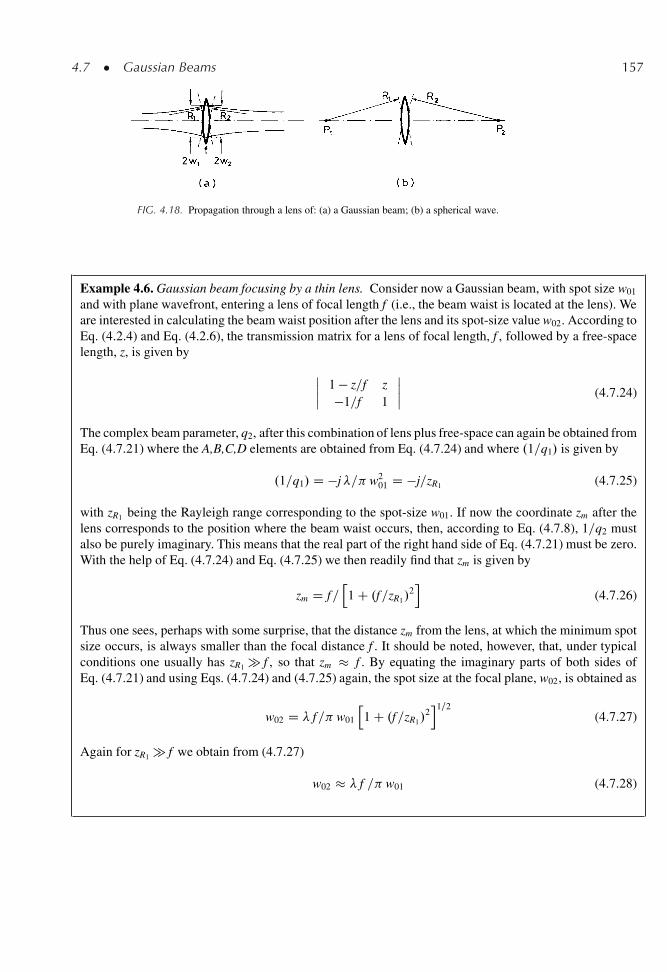
4.7 � Gaussian Beams 157
FIG. 4.18. Propagation through a lens of: (a) a Gaussian beam; (b) a spherical wave.
Example 4.6. Gaussian beam focusing by a thin lens. Consider now a Gaussian beam, with spot size w01
and with plane wavefront, entering a lens of focal length f (i.e., the beam waist is located at the lens). Weare interested in calculating the beam waist position after the lens and its spot-size value w02. According toEq. (4.2.4) and Eq. (4.2.6), the transmission matrix for a lens of focal length, f , followed by a free-spacelength, z, is given by
ˇˇ 1 � z=f z
�1=f 1
ˇˇ (4.7.24)
The complex beam parameter, q2, after this combination of lens plus free-space can again be obtained fromEq. (4.7.21) where the A,B,C,D elements are obtained from Eq. (4.7.24) and where .1=q1/ is given by
.1=q1/ D �j�= w201 D �j=zR1 (4.7.25)
with zR1 being the Rayleigh range corresponding to the spot-size w01. If now the coordinate zm after thelens corresponds to the position where the beam waist occurs, then, according to Eq. (4.7.8), 1=q2 mustalso be purely imaginary. This means that the real part of the right hand side of Eq. (4.7.21) must be zero.With the help of Eq. (4.7.24) and Eq. (4.7.25) we then readily find that zm is given by
zm D f=h1 C .f=zR1/
2i
(4.7.26)
Thus one sees, perhaps with some surprise, that the distance zm from the lens, at which the minimum spotsize occurs, is always smaller than the focal distance f . It should be noted, however, that, under typicalconditions one usually has zR1 � f , so that zm � f . By equating the imaginary parts of both sides ofEq. (4.7.21) and using Eqs. (4.7.24) and (4.7.25) again, the spot size at the focal plane, w02, is obtained as
w02 D � f= w01
h1 C .f=zR1/
2i1=2
(4.7.27)
Again for zR1 � f we obtain from (4.7.27)
w02 � � f = w01 (4.7.28)
158 4 � Ray and Wave Propagation Through Optical Media
4.7.4. Higher-Order Modes
We now return to the problem considered in sect. 4.7.1 and ask ourselves whether thereare other eigensolutions of Eq. (4.6.8), for free-space, or of Eq. (4.6.9) for a general opticalsystem. The answer is again positive and one can show that a particularly useful set of eigen-solutions can be written as the product of a Hermite polynomial with a Gaussian function. Infact, with reference to Fig. 4.14, let us assume that
u.x1, y1, z1/ D Hl
hp2x1=w1
iHm
hp2y1=w1
iexp
��jkx2
1 C y21
�=2q1
(4.7.29)
where Hl and Hm are Hermite polynomials of order l and m, q1 is the complex beam parameterat z D z1 and w1 is the corresponding spot size. Substitution of Eq. (4.7.29) in the right handside of Eq. (4.6.9) gives
u.x, y, z/ D�
1
A C .B=q1/
� 1ClCm
Hl
p2x
w
!Hm
p2y
w
!� exp �jk
x2 C y2
�2q
(4.7.30)
where q is the complex beam parameter after the optical system of Fig. 4.14 as given byEq. (4.7.4), and w is the corresponding spot size.
For free space propagation, if we let the z1 plane be the waist plane then one hasq1 D j w2
0=�, where w0 is the spot size at the beam waist. On substituting the previousexpression for q1 into Eq. (4.7.30) and using Eq. (4.7.8) we obtain
ul,m.x, y, z/ D .w=w0/Hl�21=2x=w
Hm
�21=2y=w
exp
�� x2 C y2�=w2
� exp
˚�j�kx2 C y2
�=2R
C j.1 C l C m/�� (4.7.31)
where � is again given by Eq. (4.7.15a) and where, using Eq. (4.7.11) to obtain q D q.z/, it isseen that w and R are again given by Eqs. (4.7.13a) and (4.7.13b).
The lowest order mode is obtained from Eq. (4.7.31) on setting l D m D 0. Since theHermite polynomial of zeroth order is a constant, Eq. (4.7.31) reduces to the Gaussian solutionalready discussed in sect. 4.7.1. [see Eq. (4.7.15)]. This solution is called the TEM00 mode,where TEM stands for Transverse Electric and Magnetic (within the paraxial approximationboth the electric and magnetic fields of the e.m. wave are approximately transverse to thez-direction) and where the indices 00 indicate zeroth order polynomials for both Hl and Hm
in Eq. (4.7.31). The radial intensity profile of a TEM00 Gaussian mode, at any z-coordinate,will then be I00.x, y/ / ju00j2 / exp
��2.x2 C y2/=w2
and will only depend on the radialcoordinate r D .x2 C y2/1=2. The mode thus corresponds to a circular spot [Fig. 4.19].
The next higher order mode is obtained from Eq. (4.7.31) by setting l D 1 and m D 0(or l D 0 and m D 1). Since H1 .x/ / x, the field amplitude is now given by ju10j / x �exp � �.x2 C y2/=w2
. Thus, at a given x, the field profile will be described by a Gaussian
function [see Fig. 4.15a] along the y-coordinate while, at a given y, it is described by thefunction x exp � x2=w2
�along the x-coordinate. This function, normalized to its peak value,
is plotted vs x/w in Fig. 4.15b. This mode is called TEM10 and a picture of the correspondingintensity profile is shown in Fig. 4.19. The TEM01 Œl D 0 and m D 1�, is obtained simply byrotating the picture of the TEM10 mode in Fig. 4.19 by 90ı.
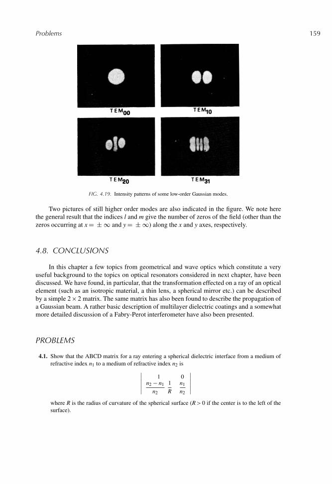
Problems 159
FIG. 4.19. Intensity patterns of some low-order Gaussian modes.
Two pictures of still higher order modes are also indicated in the figure. We note herethe general result that the indices l and m give the number of zeros of the field (other than thezeros occurring at x D ˙ 1 and y D ˙ 1) along the x and y axes, respectively.
4.8. CONCLUSIONS
In this chapter a few topics from geometrical and wave optics which constitute a veryuseful background to the topics on optical resonators considered in next chapter, have beendiscussed. We have found, in particular, that the transformation effected on a ray of an opticalelement (such as an isotropic material, a thin lens, a spherical mirror etc.) can be describedby a simple 2 � 2 matrix. The same matrix has also been found to describe the propagation ofa Gaussian beam. A rather basic description of multilayer dielectric coatings and a somewhatmore detailed discussion of a Fabry-Perot interferometer have also been presented.
PROBLEMS
4.1. Show that the ABCD matrix for a ray entering a spherical dielectric interface from a medium ofrefractive index n1 to a medium of refractive index n2 is
ˇˇˇ
1 0n2 � n1
n2
1
R
n1
n2
ˇˇˇ
where R is the radius of curvature of the spherical surface (R> 0 if the center is to the left of thesurface).
160 4 � Ray and Wave Propagation Through Optical Media
4.2. Considering a thin lens of refractive index n2 as a sequence of two, closely spaced, sphericaldielectric interfaces of radii R1 and R2 and using the result of Problem 4.1, show that its focallength is given by the relation
1
fD n2 � n1
n1
�� 1
R1C 1
R2
�
where n1 is the refractive index of the medium surrounding the lens.
4.3. A Fabry-Perot interferometer is made up of two identical mirrors with the same power reflectivity,R D 0.99, and same fractional internal power loss, A D 0.005. Calculate the peak transmission andthe finesse of the interferometer.
4.4. A Fabry-Perot interferometer, made up of two identical mirrors, air-spaced by a distance L, isilluminated by a monochromatic e.m. wave of tunable-frequency. From the measurement of thetransmitted intensity versus the frequency of the input wave one finds that the free spectral rangeof the interferometer is 3 � 109 Hz and its resolution is 60 MHz. Calculate the spacing L of theinterferometer, its finesse and the mirror reflectivity. If the peak transmission is 50%, calculatealso the mirror loss.
4.5. A Fabry-Perot interferometer, made up of two identical mirrors air-spaced by a distance L, isilluminated by a 1-ps pulse from an external source at the wavelength λ Š 600 nm. The outputbeam is observed to be made of a regular sequence of 1-ps pulses spaced by 10 ns. The energy ofthe pulses decreases exponentially with time with a time constant of 100 ns. Calculate the cavitylength and the mirror reflectivity.
4.6. By direct substitution of Eq. (4.7.2) into the right hand side of Eq. (4.6.9) show that the doubleintegral appearing in Eq. (4.6.9), when taken between �1 and C1, gives Eq. (4.7.3) where q isrelated to q0 by Eq. (4.7.4).
4.7. A positive lens of focal length f is placed at a distance d from the waist of a TEM00 beam, of waistspot size w0. Derive the expression for the focal length f (in terms of w0 and d) that is required inorder that the beam, leaving the lens, has a plane wavefront.
4.8. Show that the power contained in a TEM00 Gaussian beam of spot size w is given byP D �
� w2=2�
Ip where Ip is the peak .r D 0/ intensity of the beam.
4.9. A given He-Ne laser, oscillating in a pure Gaussian TEM00 mode at λ D 632.8 nm with an outputpower of P D 5 mW is advertised as having a far-field divergence angle of 1 mrad. Calculate thespot size, the peak intensity and the peak electric field at the waist position.
4.10. The beam of an Ar laser, oscillating in a pure Gaussian TEM00 mode at λ D 514.5 nm with anoutput power of 1 W, is sent to a target at a distance of 100 m from the beam waist. If the spotsize at the beam waist is w0 D 2 mm, calculate, at the target position, the spot size, the radius ofcurvature of the phase front and the peak intensity.
4.11. Consider a TEM00 Gaussian beam of spot size w1 entering a lens of diameter D and focal length f .To avoid excessive diffraction effects at the lens edge, due to truncation of the Gaussian field by thelens, one usually chooses the lens diameter according to the criterion D � 2.25 w1. Assume that:(i) the equality holds in the previous expression; (ii) the waist of the incident beam is located at thelens, i.e. w1 D w01; (iii) f � zR1 D�w2
01=�; (iv) Eq. (4.7.27) is still valid. Under these conditions,express the minimum spot size after the lens as a function of the lens numerical aperture N.A.[N.A. D sin � , where � D tan�1.D=f /, so that, for small � , N.A. Š .D=f /].
References 161
4.12. Suppose that a TEM00 Gaussian beam from a Ruby laser .�D 694.3 nm/ is transmitted through a1 m diameter diffraction-limited telescope to illuminate a spot on the face of the moon. Assumingan earth-moon distance of z Š 348,000 km and using the relation D D 2.25 w01 between telescopeobjective diameter and beam spot size (see previous problem) calculate the beam spot size on themoon (distortion effects from the atmosphere can be important, but are neglected here).
4.13. A Gaussian beam of waist spot size w0 is passed through a solid plate of transparent material oflength, L, and refractive index n. The plate is placed just in front of the beam waist. Using theABCD law of Gaussian beam propagation, show that the spot size and radius of curvature of thephase front after the plate are the same as for propagation, in a vacuum, over a distance L0 D L=n.According to this result, is the far-field divergence angle affected by the insertion of the plate?
4.14. From Eq. (4.7.26) show that a Gaussian beam of waist spot size w01 cannot be focused at a distancelarger than zR1=2, where zR1 D� w2
01=�. What is the focal length corresponding to this maximumfocusing condition?
References
1. H. Kogelnik, Propagation of Laser Beams, in Applied Optics and Optical Engineering, ed. by R. Shannon andJ.C. Wynant (Academic Press, New York, 1979), Vol. II, pp. 156–190.
2. M. Born and E. Wolf, Principles of Optics, 6th edition (Pergamon, Oxford, 1980) Sect. 1.5.3. E. Ritter, Coatings and Thin-Film Techniques, in Laser Handbook, ed. by F.T. Arecchi and E.O. Schultz-Dubois
(North-Holland, Amsterdam, 1972) Vol. 1, pp. 897–921.4. Thin Films for Optical Systems, ed. by F. R. Flory (Marcel Dekker, New York 1995).5. Ref. [2], sect. 7.6.6. A.E. Siegman, Lasers (Oxford University Press, Oxford, U. K.), Chapt. 16.7. Ref. [6], chapt. 20.8. H. Kogelnik ant T. Li, Laser Beams and Resonators, Appl. Opt. 5, 1550 (1966).
5
Passive Optical Resonators
5.1. INTRODUCTION
This chapter deals with the theory of passive optical resonators i.e. where no activemedium is present within the cavity. The most widely used laser resonators have either planeor spherical mirrors of rectangular (or, more often, circular) shape, separated by some dis-tance L. Typically, L may range from a few centimeters to a few tens of centimeters, whilethe mirror dimensions range from a fraction of a centimeter to a few centimeters. Laser res-onators thus differ from those used in the microwave field (see e.g. Sect. 2.2.1) in two mainrespects: (1) The resonator dimensions are much greater than the laser wavelength. (2) Res-onators are usually open, i.e. no lateral surfaces are used. The resonator length is usually muchgreater than the laser wavelength because this wavelength usually ranges from a fraction of amicrometer to a few tens of micrometers. A laser cavity with length comparable to the wave-length would then generally have too low a gain to allow laser oscillation. Laser resonatorsare usually open because this drastically reduces the number of modes which can oscillatewith low loss. In fact, with reference to example 5.1 to be considered below, it is seen thateven a narrow linewidth laser such as a He-Ne laser would have a very large number of modes.�109/ if the resonator were closed. By contrast, on removing the lateral surfaces, the numberof low-loss modes reduces to just a few (�6 in the example). In these open resonators, in fact,only the very few modes corresponding to a superposition of waves traveling nearly parallelto the resonator axis will have low enough losses to allow laser oscillation.
According to the previous discussion, it is seen that open resonators have inevitably somelosses due to diffraction of the e.m. field, which leads to some fraction of the energy leavingthe sides of the cavity (diffraction losses). Strictly speaking, therefore, the mode definitiongiven in Sect. 2.2.1 cannot be applied to an open resonator and true modes (i.e. stationaryconfigurations) do not exist for such a resonator. In what follows, however, we shall see thatstanding-wave configurations having very small losses do exist in open resonators. We will
O. Svelto, Principles of Lasers,c
163DOI: 10.1007/978-1-4419-1302-9 5, � Springer Science+Business Media LLC 2010
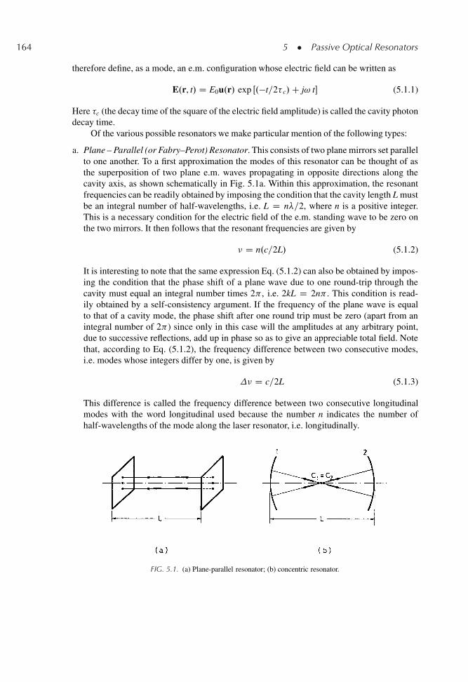
164 5 � Passive Optical Resonators
therefore define, as a mode, an e.m. configuration whose electric field can be written as
E.r, t/ D E0u.r/ exp Œ.�t=2� c/C j! t� (5.1.1)
Here �c (the decay time of the square of the electric field amplitude) is called the cavity photondecay time.
Of the various possible resonators we make particular mention of the following types:
a. Plane – Parallel (or Fabry–Perot) Resonator. This consists of two plane mirrors set parallelto one another. To a first approximation the modes of this resonator can be thought of asthe superposition of two plane e.m. waves propagating in opposite directions along thecavity axis, as shown schematically in Fig. 5.1a. Within this approximation, the resonantfrequencies can be readily obtained by imposing the condition that the cavity length L mustbe an integral number of half-wavelengths, i.e. L D n�=2, where n is a positive integer.This is a necessary condition for the electric field of the e.m. standing wave to be zero onthe two mirrors. It then follows that the resonant frequencies are given by
� D n.c=2L/ (5.1.2)
It is interesting to note that the same expression Eq. (5.1.2) can also be obtained by impos-ing the condition that the phase shift of a plane wave due to one round-trip through thecavity must equal an integral number times 2 , i.e. 2kL D 2n . This condition is read-ily obtained by a self-consistency argument. If the frequency of the plane wave is equalto that of a cavity mode, the phase shift after one round trip must be zero (apart from anintegral number of 2 ) since only in this case will the amplitudes at any arbitrary point,due to successive reflections, add up in phase so as to give an appreciable total field. Notethat, according to Eq. (5.1.2), the frequency difference between two consecutive modes,i.e. modes whose integers differ by one, is given by
� D c=2L (5.1.3)
This difference is called the frequency difference between two consecutive longitudinalmodes with the word longitudinal used because the number n indicates the number ofhalf-wavelengths of the mode along the laser resonator, i.e. longitudinally.
FIG. 5.1. (a) Plane-parallel resonator; (b) concentric resonator.
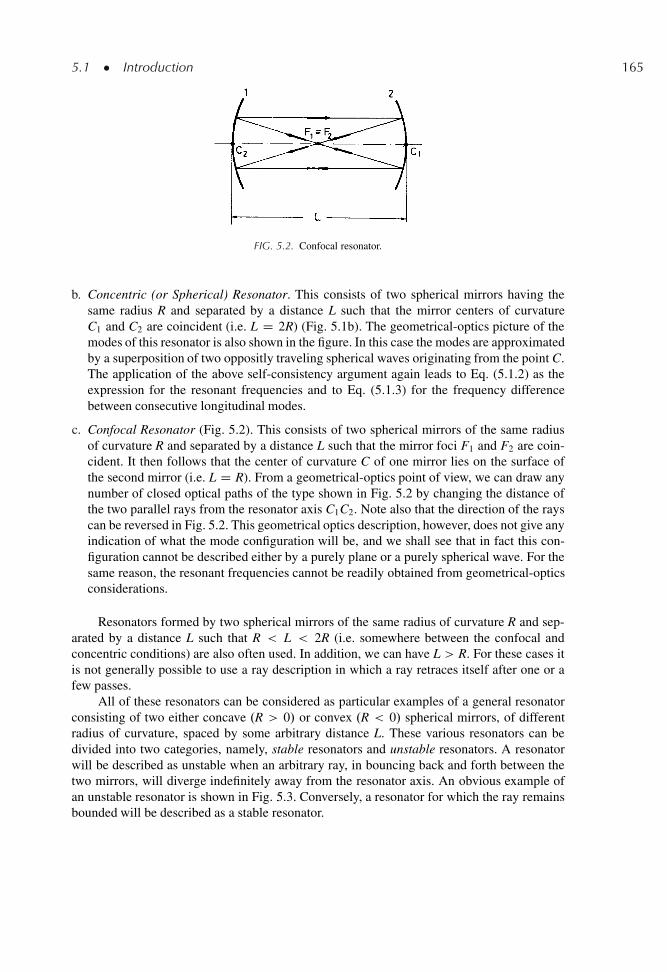
5.1 � Introduction 165
FIG. 5.2. Confocal resonator.
b. Concentric (or Spherical) Resonator. This consists of two spherical mirrors having thesame radius R and separated by a distance L such that the mirror centers of curvatureC1 and C2 are coincident (i.e. L D 2R) (Fig. 5.1b). The geometrical-optics picture of themodes of this resonator is also shown in the figure. In this case the modes are approximatedby a superposition of two oppositly traveling spherical waves originating from the point C.The application of the above self-consistency argument again leads to Eq. (5.1.2) as theexpression for the resonant frequencies and to Eq. (5.1.3) for the frequency differencebetween consecutive longitudinal modes.
c. Confocal Resonator (Fig. 5.2). This consists of two spherical mirrors of the same radiusof curvature R and separated by a distance L such that the mirror foci F1 and F2 are coin-cident. It then follows that the center of curvature C of one mirror lies on the surface ofthe second mirror (i.e. L D R). From a geometrical-optics point of view, we can draw anynumber of closed optical paths of the type shown in Fig. 5.2 by changing the distance ofthe two parallel rays from the resonator axis C1C2. Note also that the direction of the rayscan be reversed in Fig. 5.2. This geometrical optics description, however, does not give anyindication of what the mode configuration will be, and we shall see that in fact this con-figuration cannot be described either by a purely plane or a purely spherical wave. For thesame reason, the resonant frequencies cannot be readily obtained from geometrical-opticsconsiderations.
Resonators formed by two spherical mirrors of the same radius of curvature R and sep-arated by a distance L such that R < L < 2R (i.e. somewhere between the confocal andconcentric conditions) are also often used. In addition, we can have L > R. For these cases itis not generally possible to use a ray description in which a ray retraces itself after one or afew passes.
All of these resonators can be considered as particular examples of a general resonatorconsisting of two either concave .R > 0/ or convex .R < 0/ spherical mirrors, of differentradius of curvature, spaced by some arbitrary distance L. These various resonators can bedivided into two categories, namely, stable resonators and unstable resonators. A resonatorwill be described as unstable when an arbitrary ray, in bouncing back and forth between thetwo mirrors, will diverge indefinitely away from the resonator axis. An obvious example ofan unstable resonator is shown in Fig. 5.3. Conversely, a resonator for which the ray remainsbounded will be described as a stable resonator.
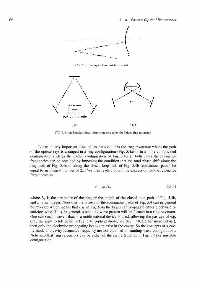
166 5 � Passive Optical Resonators
FIG. 5.3. Example of an unstable resonator.
FIG. 5.4. (a) Simplest three-mirror ring resonator. (b) Folded ring resonator.
A particularly important class of laser resonator is the ring resonator where the pathof the optical rays is arranged in a ring configuration (Fig. 5.4a) or in a more complicatedconfiguration such as the folded configuration of Fig. 5.4b. In both cases the resonancefrequencies can be obtained by imposing the condition that the total phase shift along thering path of Fig. 5.4a or along the closed-loop path of Fig. 5.4b (continuous paths) beequal to an integral number of 2 . We then readily obtain the expression for the resonancefrequencies as
� D nc=Lp (5.1.4)
where Lp is the perimeter of the ring or the length of the closed-loop path of Fig. 5.4b,and n is an integer. Note that the arrows of the continuous paths of Fig. 5.4 can in generalbe reversed which means that e.g. in Fig. 5.4a the beam can propagate either clockwise oranticlockwise. Thus, in general, a standing wave pattern will be formed in a ring resonator.One can see, however, that, if a unidirectional device is used, allowing the passage of e.g.only the right to left beam in Fig. 5.4a (optical diode, see Sect. 7.8.2.2. for more details),then only the clockwise propagating beam can exist in the cavity. So the concepts of a cav-ity mode and cavity resonance frequency are not confined to standing-wave configurations.Note also that ring resonators can be either of the stable (such as in Fig. 5.4) or unstableconfiguration.
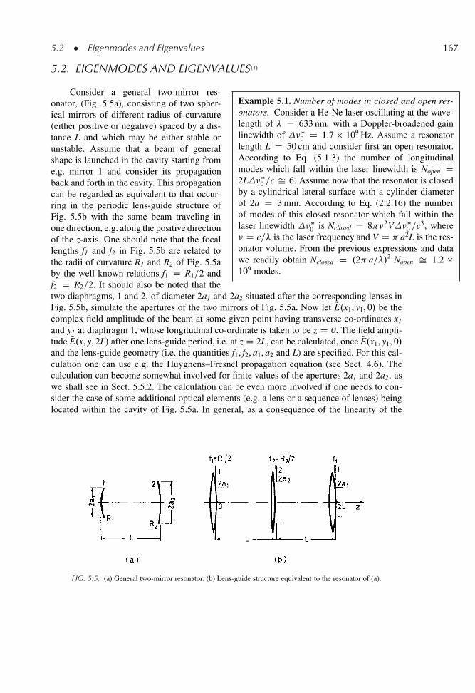
5.2 � Eigenmodes and Eigenvalues 167
5.2. EIGENMODES AND EIGENVALUES.1/
Example 5.1. Number of modes in closed and open res-onators. Consider a He-Ne laser oscillating at the wave-length of � D 633 nm, with a Doppler-broadened gainlinewidth of ��
0 D 1.7 � 109 Hz. Assume a resonatorlength L D 50 cm and consider first an open resonator.According to Eq. (5.1.3) the number of longitudinalmodes which fall within the laser linewidth is Nopen D2L��
0 =c Š 6. Assume now that the resonator is closedby a cylindrical lateral surface with a cylinder diameterof 2a D 3 mm. According to Eq. (2.2.16) the numberof modes of this closed resonator which fall within thelaser linewidth ��
0 is Nclosed D 8 �2V��0 =c3, where
� D c=� is the laser frequency and V D a2L is the res-onator volume. From the previous expressions and datawe readily obtain Nclosed D .2 a=�/2 Nopen Š 1.2 �109 modes.
Consider a general two-mirror res-onator, (Fig. 5.5a), consisting of two spher-ical mirrors of different radius of curvature(either positive or negative) spaced by a dis-tance L and which may be either stable orunstable. Assume that a beam of generalshape is launched in the cavity starting frome.g. mirror 1 and consider its propagationback and forth in the cavity. This propagationcan be regarded as equivalent to that occur-ring in the periodic lens-guide structure ofFig. 5.5b with the same beam traveling inone direction, e.g. along the positive directionof the z-axis. One should note that the focallengths f1 and f2 in Fig. 5.5b are related tothe radii of curvature R1 and R2 of Fig. 5.5aby the well known relations f1 D R1=2 andf2 D R2=2. It should also be noted that thetwo diaphragms, 1 and 2, of diameter 2a1 and 2a2 situated after the corresponding lenses inFig. 5.5b, simulate the apertures of the two mirrors of Fig. 5.5a. Now let QE.x1, y1, 0/ be thecomplex field amplitude of the beam at some given point having transverse co-ordinates x1
and y1 at diaphragm 1, whose longitudinal co-ordinate is taken to be z D 0. The field ampli-tude QE.x, y, 2L/ after one lens-guide period, i.e. at z D 2L, can be calculated, once QE.x1, y1, 0/and the lens-guide geometry (i.e. the quantities f1, f2, a1, a2 and L) are specified. For this cal-culation one can use e.g. the Huyghens–Fresnel propagation equation (see Sect. 4.6). Thecalculation can become somewhat involved for finite values of the apertures 2a1 and 2a2, aswe shall see in Sect. 5.5.2. The calculation can be even more involved if one needs to con-sider the case of some additional optical elements (e.g. a lens or a sequence of lenses) beinglocated within the cavity of Fig. 5.5a. In general, as a consequence of the linearity of the
FIG. 5.5. (a) General two-mirror resonator. (b) Lens-guide structure equivalent to the resonator of (a).
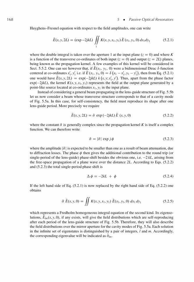
168 5 � Passive Optical Resonators
Huyghens–Fresnel equation with respect to the field amplitudes, one can write
QE.x, y, 2L/ D .exp �2jkL/“1
K.x, y, x1, y1/ QE .x1, y1, 0/ dx1dy1 (5.2.1)
where the double integral is taken over the aperture 1 at the input plane .z D 0/ and where Kis a function of the transverse co-ordinates of both input .z D 0/ and output .z D 2L/ planes,being known as the propagation kernel. A few examples of this kernel will be considered inSect. 5.5.2. One can see however that, if QE.x1, y1, 0/ were a bidimensional Dirac ı-functioncentered at co-ordinates x0
1, y01 i.e. if QE .x1, y1, 0/ D ı
x1 � x0
1, y1 � y01
�, then from Eq. (5.2.1)
one would have QE.x, y, 2L/ D exp.�2jkL/ kx, y; x0
1, y0�. Thus, apart from the phase factorexp.�2jkL/, the kernel K.x, y, x1, y1/ represents the field at the output plane generated by apoint-like source located at co-ordinates x1, y1 in the input plane.
Instead of considering a general beam propagating in the lens-guide structure of Fig. 5.5blet us now consider a beam whose transverse structure corresponds to that of a cavity modeof Fig. 5.5a. In this case, for self-consistency, the field must reproduce its shape after onelens-guide period. More precisely we require
QE.x, y, 2L/ D Q� exp .�2jkL/ QE .x, y, 0/ (5.2.2)
where the constant Q� is generally complex since the propagation kernel K is itself a complexfunction. We can therefore write
Q� D j Q� j exp j� (5.2.3)
where the amplitude j Q� j is expected to be smaller than one as a result of beam attenuation, dueto diffraction losses. The phase � then gives the additional contribution to the round trip (orsingle-period of the lens-guide) phase-shift besides the obvious one, i.e. �2 kL, arising fromthe free-space propagation of a plane wave over the distance 2L. According to Eqs. (5.2.2)and (5.2.3) the total single-period phase shift is
�� D �2kL C � (5.2.4)
If the left hand side of Eq. (5.2.1) is now replaced by the right hand side of Eq. (5.2.2) oneobtains
Q� QE.x, y, 0/ D“
K.x, y, x1, y1/ QE.x1, y1, 0/ dx1 dy1 (5.2.5)
which represents a Fredholm homogeneous integral equation of the second kind. Its eigenso-lutions, QElm.x, y, 0/, if any exists, will give the field distributions which are self-reproducingafter each period of the lens-guide structure of Fig. 5.5b. Therefore, they will also describethe field distributions over the mirror aperture for the cavity modes of Fig. 5.5a. Each solutionin the infinite set of eigenstates is distinguished by a pair of integers, l and m. Accordingly,the corresponding eigenvalue will be indicated as Q�lm.
5.3 � Photon Lifetime and Cavity Q 169
From the above discussion, the eigenvalues Q�lm are seen to be such that j Q�lmj2 gives thefactor by which the beam intensity is changed as a result of one round trip. Since this changeis due to diffraction losses, we must then have j Q�lmj2 < 1j thus the quantity
�l m D 1 � j Q�l m j 2 (5.2.6)
gives the round-trip fractional power loss due to diffraction. One can also see that, accordingto Eq. (5.2.4), ��lm D �2 kL C �lm is the corresponding round-trip phase shift. For the fieldto be self-reproducing, we must then require that �lm D �2 n, where n is an integer. Wethus get �2kL C �lm D �2πn, and, with the substitution k D 2π�=c, we obtain the cavityresonance frequencies as
�lmn D c
2L
�n C �lm
2
�(5.2.7)
Note that we have indicated explicitly that these frequencies are dependent on the values ofthe three numbers l, m, and n. The integers l and m represent the order of the eigensolutionin Eq. (5.2.5) while the integer number n specifies the total phase shift of the beam, after oneround trip, in units of 2π (i.e. n D ���lm=2 ).
As a conclusion of this section we can say that the eigenmodes and the eigenvaluesof our problem can be obtained upon solving the integral equation Eq. (5.2.5). In fact, itseigensolutions, QElm, give the field of the eigenmodes at all point in a given plane. For eachmode QElm, the corresponding eigenvalue Q�lm then gives: (a) The round-trip diffraction loss,�lm, through its magnitude j Q�lmj [see Eq. (5.2.6)]. (b) The resonance frequency, �lmn, throughits phase, �lm [see Eq. (5.2.7)].
5.3. PHOTON LIFETIME AND CAVITY Q
Consider a given mode of a stable or unstable cavity and assume, for generality, thatsome losses other than diffraction losses are also present. For instance one may have mirrorlosses as a result of mirror reflectivity being smaller than unity. One may also have scatteringlosses in some optical element within the cavity. Under these conditions we want to calculatethe rate of energy decay in the given cavity mode. To this purpose, let I0 be the initial intensitycorresponding to the field amplitude QE.x1, y1, 0/ at a given transverse coordinate x1, y1. LetR1 and R2 be the (power) reflectivities of the two mirrors and Ti the fractional internal lossper pass due to diffraction and any other internal losses. The intensity I.t1/ at the same pointx1, y1 at a time t1 D 2L=c, i.e. after one cavity round trip, will be
I.t1/ D R1 R2.1 � Ti/2 I0 (5.3.1)
Note that, since Ti is defined here as the fractional internal loss per pass, the intensity isreduced by a factor .1 � Ti/ in a single pass and hence by a factor .1 � Ti/
2 in a double pass(round trip). The intensity, at the same transverse co-ordinate, after m round trips, i.e. at time
tm D 2mL=c (5.3.2)
170 5 � Passive Optical Resonators
is then
I.tm/ D ŒR1R2.1 � Ti/2�m I0 (5.3.3)
Let now �.t/ be the total number of photons in the given cavity mode at time t. Since themode retains its shape after each round trip, we can set �.t/ / I.t/. From Eq. (5.3.3) we canthen write
�.tm/ D �R1 R2 .1 � Ti/
2m� 0 (5.3.4)
where �0 is the number of photons initially present in the cavity. We can also set
�.tm/ D Œexp.�t=�c/��0 (5.3.5)
where �c is a suitable constant. In fact, a comparison of Eqs. (5.3.5) with (5.3.4) with the helpof Eq. (5.3.2) shows that
exp .� 2mL=c �c/ D �R1 R2 .1 � Ti/
2m(5.3.6)
from which one finds that �c is independent of the number of round trips, m, and is given by
�c D �2 L=c ln�R1 R2.1 � Ti/
2
(5.3.7)
If we now assume that Eq. (5.3.5) holds, not only at times tm, but also at any time t .>0/, wecan then write
�.t/ Š exp .�t=�c/ �0 (5.3.8)
Example 5.2. Calculation of the cavity photon lifetime.We will assume R1 D R2 D R D 0.98 and Ti Š 0. FromEq. (5.3.7) we obtain �c D �T=Œ� ln R� D 49.5 �T , where�T is the transit time of the photons for a single-pass inthe cavity. From this example we note that the photon life-time is much longer than the transit time, a result which istypical of low loss cavities. If we now assume L D 90 cm,we get �T D 3 ns and �c Š 150 ns.
In this way, we justify the assumptionEq. (5.1.1) for the mode field and iden-tify Eq. (5.3.7) as the expression for thecavity photon lifetime. One can notice thatEq. (5.3.7), with the help of Eqs. (1.2.4)and (1.2.6), can readily be transformed to
�c D L=c� (5.3.9)
We thus see that the cavity photon lifetimeis just equal to the transit time �T D L=c of the beam in the laser cavity divided by the(logarithmic) cavity loss � .
Having calculated the photon lifetime, the time behavior of the electric field, at any pointinside the resonator can, according to Eq. (5.1.1) and within the scalar approximation, bewritten as E.t/ D QE exp Œ.�t=2�c/C j!t�, where ! is the angular resonance frequency ofthe mode. The same time behavior then applies for the field of the output wave leaving thecavity through one mirror as a result of finite mirror transmission. If we now take the Fouriertransform of this field, we find that the power spectrum of the emitted light has a Lorentzianline shape with linewidth (FWHM) given by
��c D 1=2 �c (5.3.10)
5.4 � Stability Condition 171
Example 5.3. Linewidth of a cavity resonance. If we takeagain R1 D R2 D 0.98 and Ti D 0, from Eqs. (5.3.10) and(5.3.7) we get�c Š 6.4307�10�3�.c=2L/, while fromEq. (4.5.12) we get �c Š 6.4308 � 10�3 � .c=2L/. Forthe particular case L D 90 cm, we then obtain �c Š1.1 MHz. Even at the relatively low reflectivity values ofR1 D R2 D 0.5, the discrepancy is not large. In fact fromEqs. (5.3.10) and (5.3.7) we get �c Š 0.221 � .c=2L/,while from Eq. (4.5.12) �c Š 0.225 � .c=2L/. Againfor L D 90 cm we then obtain �c Š 37.5 MHz. Thus,in typical cases, �c may range from a few to a few tensof MHz.
It should be noted that the spectrum of theemitted light, obtained in this way, does notexactly agree with the transmission spectrumshown for a Fabry–Perot interferometer inSect. 4.5, whose shape is not Lorentzian [seeEq. (4.5.6)]. In particular, the expression for�c obtained here [see Eq. (5.3.10)], whencombined with Eq. (5.3.7) with Ti Š 0, doesnot coincide with that obtained in Sect. 4.5[see Eq. (4.5.12) with L0 D L]. This discrep-ancy can be traced back to the approximationmade in writing Eq. (5.3.8). In numericalterms, however, the discrepancy between thetwo results is quite small, especially at highvalues of reflectivity, as can be seen from the following example. From now on we will there-fore assume that the cavity line shape is Lorentzian with width given by Eq. (5.3.10) and thatthe cavity photon lifetime is given by Eq. (5.3.7).
Having discussed the cavity photon lifetime, we can now introduce the cavity qualityfactor, or Q factor, and derive its relation to the photon lifetime. For any resonant system, andin particular for a resonant optical cavity, one defines the cavity Q factor (usually abbreviatedto cavity Q) as Q D 2 (energy stored)/(energy lost in one cycle of oscillation). Thus a highvalue of cavity Q implies low losses of the resonant system. Since, in our case, the energystored is �hv and the energy lost in one cycle is h�.�d�=dt/.1=�/ D �hd�=dt, we have
Q D �2 ��=.d�=dt/ (5.3.11)
From Eq. (5.3.8) we then get
Q D 2 ��c (5.3.12)
Example 5.4. Q-factor of a laser cavity According toexample 5.2 we will again take �c Š 150 ns and assume� Š 5 � 1014 Hz (i.e. � Š 630 nm). From Eq. (5.3.12) weobtain Q D 4.7 � 108. Thus, very high Q-values can beachieved in a laser cavity and this means that a very smallfraction of the energy is lost during one oscillation cycle
which, with the help of Eq. (5.3.10), can betransformed to the more suggestive form
Q D �=��c (5.3.13)
Thus the cavity Q factor can be interpreted asthe ratio between the resonance frequency, �,of the given mode and its linewidth, ��c.
5.4. STABILITY CONDITION
Consider first a general two-mirror resonator (Fig. 5.6a) and a ray leaving point P0 of aplane ˇ inside the resonator e.g. just in front of mirror 1. This ray, after reflection from mirrors2 and 1, will intersect the plane ˇ at some point P1. If we let r0 and r1 be the transverse
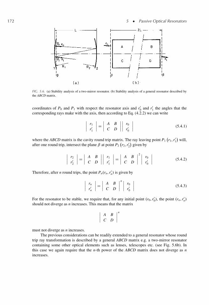
172 5 � Passive Optical Resonators
FIG. 5.6. (a) Stability analysis of a two-mirror resonator. (b) Stability analysis of a general resonator described bythe ABCD matrix.
coordinates of P0 and P1 with respect the resonator axis and r00 and r0
1 the angles that thecorresponding rays make with the axis, then according to Eq. (4.2.2) we can write
ˇˇ r1
r01
ˇˇ D
ˇˇ A B
C D
ˇˇˇˇ r0
r00
ˇˇ (5.4.1)
where the ABCD matrix is the cavity round trip matrix. The ray leaving point P1r1, r0
1
�will,
after one round trip, intersect the plane ˇ at point P2r2, r0
2
�given by
ˇˇ r2
r02
ˇˇ D
ˇˇ A B
C D
ˇˇˇˇ r1
r01
ˇˇ D
ˇˇ A B
C D
ˇˇ
2 ˇˇ r0
r00
ˇˇ (5.4.2)
Therefore, after n round trips, the point Pn.rn, r0n/ is given by
ˇˇ rn
r0n
ˇˇ D
ˇˇ A B
C D
ˇˇ n ˇˇ r0
r00
ˇˇ (5.4.3)
For the resonator to be stable, we require that, for any initial point .r0, r00/, the point .rn, r0
n/
should not diverge as n increases. This means that the matrix
ˇˇ A B
C D
ˇˇ n
must not diverge as n increases.The previous considerations can be readily extended to a general resonator whose round
trip ray transformation is described by a general ABCD matrix e.g. a two-mirror resonatorcontaining some other optical elements such as lenses, telescopes etc. (see Fig. 5.6b). Inthis case we again require that the n-th power of the ABCD matrix does not diverge as nincreases.
5.4 � Stability Condition 173
For both resonators shown in Fig. 5.6a, b the ray starts from and arrives at the same planeˇ, which means that the refractive index is the same for both rays, input, r0, and output, r1. Itthen follows that the determinant of the matrix, AD-BC, has unit value. A theorem of matrixcalculus,.2/ sometimes referred to as Sylvester’s theorem, then shows that, if we define anangle by the relation
cos D .A C D/=2 (5.4.4)
one has
ˇˇ A B
C D
ˇˇ n
D 1
sin
ˇˇ A sin n � sin.n � 1/ B sin n
C sin n D sin n � sin.n � 1/
ˇˇ (5.4.5)
Equation (5.4.5) shows that the n-th power matrix does not diverge if is a real quan-tity. Indeed, if were complex, say D a C ib, the terms proportional to e.g. sin n inEq. (5.4.5) could be written as sin n D Œexp.jn/ C exp.�jn/�=2j D Œexp.jna � nb/ Cexp.�jna C nb/�=2j. The quantity sin n would then contain a term growing exponentiallywith n, e.g. Œexp.�jna C nb/�=2j for b > 0, and the overall n-th power matrix would thusdiverge as n increases. So, for the resonator to be stable, we require to be real and, accordingto Eq. (5.4.4), this implies that
�1 <
�A C D
2
�< 1 (5.4.6)
Equation (5.4.6) establishes the stability condition for the general resonator of Fig. 5.6b.In the case of the two-mirror resonator of Fig. 5.6a we can go one step further by explic-itly calculating the corresponding ABCD matrix. We recall that a given overall matrix can beobtained by the product of matrices of the individual optical elements traversed by the beam,with the matrices written down in the reverse of the order in which the ray propagates throughthe corresponding elements. Thus, in this case, the ABCD matrix is given by the ordered prod-uct of the following four matrices: (1) Reflection from mirror 1, (2) free-space propagationfrom mirror 1 to 2, (3) reflection from mirror 2, (4) free-space propagation from mirror 2 to1. With the help of Table 4.1 we then have
ˇˇ A B
C D
ˇˇ D
ˇˇ 1 0
�2=R1 1
ˇˇˇˇ 1 L
0 1
ˇˇˇˇ 1 0
�2=R2 1
ˇˇˇˇ 1 L
0 1
ˇˇ (5.4.7)
After performing the matrix multiplication of Eq. (5.4.7), we obtain
A C D
2D 1 � 2 L
R1� 2 L
R2C 2 L2
R1 R2(5.4.8)
Equation (5.4.8) can be readily transformed to
A C D
2D 2
�1 � L
R1
��1 � L
R2
�� 1 (5.4.9)
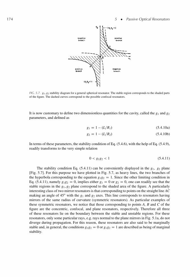
174 5 � Passive Optical Resonators
FIG. 5.7. g1, g2 stability diagram for a general spherical resonator. The stable region corresponds to the shaded partsof the figure. The dashed curves correspond to the possible confocal resonators.
It is now customary to define two dimensionless quantities for the cavity, called the g1 and g2
parameters, and defined as
g1 D 1 � .L=R1/ (5.4.10a)
g2 D 1 � .L=R2/ (5.4.10b)
In terms of these parameters, the stability condition of Eq. (5.4.6), with the help of Eq. (5.4.9),readily transforms to the very simple relation
0 < g1g2 < 1 (5.4.11)
The stability condition Eq. (5.4.11) can be conveniently displayed in the g1, g2 plane[Fig. 5.7]. For this purpose we have plotted in Fig. 5.7, as heavy lines, the two branches ofthe hyperbola corresponding to the equation g1g2 D 1. Since the other limiting condition inEq. (5.4.11), namely g1g2 D 0, implies either g1 D 0 or g2 D 0, one can readily see that thestable regions in the g1, g2 plane correspond to the shaded area of the figure. A particularlyinteresting class of two mirror resonators is that corresponding to points on the straight line ACmaking an angle of 45ı with the g1 and g2 axes. This line corresponds to resonators havingmirrors of the same radius of curvature (symmetric resonators). As particular examples ofthese symmetric resonators, we notice that those corresponding to points A, B and C of thefigure are the concentric, confocal, and plane resonators, respectively. Therefore all threeof these resonators lie on the boundary between the stable and unstable regions. For theseresonators, only some particular rays, e.g. rays normal to the plane mirrors in Fig. 5.1a, do notdiverge during propagation. For this reason, these resonators are also said to be marginallystable and, in general, the conditions g1g2 D 0 or g1g2 D 1 are described as being of marginalstability.
5.5 � Stable Resonators 175
5.5. STABLE RESONATORS
To greatly simplify our analysis we will first consider a resonator with no limitingaperture. We will then briefly consider the effects of a finite aperture.
5.5.1. Resonators with Infinite Aperture.3,4/
With reference to Fig. 5.6b for a general resonator and to 5.5a for a two-mirror resonatorwe will assume no limiting aperture i.e. we will take a1 D a2 D 1 in Fig. 5.5a. The fielddistribution u.x, y, z/ after one cavity round trip of Fig. 5.5a or after one period of the lens-guide system of Fig. 5.5b i.e. at z D 2L, can be obtained from Eq. (4.6.9) with z1 D 0,where the ABCD matrix is the one-round-trip (or one-period) matrix. If we now take, at thez1 D 0 plane, QE .x1, y1, 0/ D u .x1, y1, 0/, then, within the paraxial wave approximation andaccording to Eq. (4.6.4), we can write QE.x, y, 2L/ D u.x, y, 2L/ exp .�2jkL/. On inserting, intothis relation, the expression for u.x, y, z/ given by Eq. (4.6.9) we get
QE.x, y, 2L/ D exp .�2 jkL/
C1Z�1
C1Z�1
�i
B�
�exp
� jK
"Ax1
2 C y12�C D.x2 C y2/� 2 x1 x � 2 y1 y
2 B
#
� QE.x1, y1, 0/dx1dy1 (5.5.1)
A comparison of Eqs. (5.5.1) with (5.2.1) then shows that the propagation kernelK.x, y; x1, y1/, is given, in this case, by
K D�
j
B�
�exp �jk
"Ax1
2 C y12�C D
x2 C y2
� � 2 x1 x � 2 y1 y
2 B
#(5.5.1a)
As explained in Sect. 4.7, the lowest order Gaussian solution, Eq. (4.7.1), and the gen-eral solution for higher order, Eq. (4.7.30), are eigensolutions of the propagation equation,Eq. (4.6.9), when no aperture is present within the optical system described by the givenABCD matrix. For these Hermite–Gaussian eigensolutions to describe the field distribution ofthe cavity eigenmodes, we must now require that the beam reproduces itself after one roundtrip. This means that if we let q1 be the complex beam parameter of the Gaussian beam leavingplane ˇ in front of e.g. mirror 1 of Fig. 5.8a, the complex beam parameter q after one round-trip must be equal to q1. From the ABCD law of Gaussian beam propagation Eq. (4.7.4), if weset q1 D q, we obtain
q D Aq C B
Cq C D(5.5.2)
The q parameter must then satisfy the quadratic equation
Cq2 C .D � A/q � B D 0 (5.5.3)
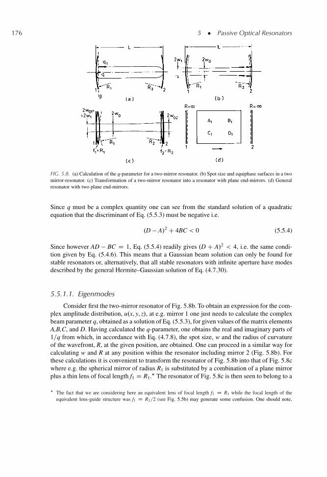
176 5 � Passive Optical Resonators
FIG. 5.8. (a) Calculation of the q-parameter for a two-mirror resonator. (b) Spot size and equiphase surfaces in a twomirror-resonator. (c) Transformation of a two-mirror resonator into a resonator with plane end-mirrors. (d) Generalresonator with two plane end-mirrors.
Since q must be a complex quantity one can see from the standard solution of a quadraticequation that the discriminant of Eq. (5.5.3) must be negative i.e.
.D � A/2 C 4BC < 0 (5.5.4)
Since however AD � BC D 1, Eq. (5.5.4) readily gives .D C A/2 < 4, i.e. the same condi-tion given by Eq. (5.4.6). This means that a Gaussian beam solution can only be found forstable resonators or, alternatively, that all stable resonators with infinite aperture have modesdescribed by the general Hermite–Gaussian solution of Eq. (4.7.30).
5.5.1.1. Eigenmodes
Consider first the two-mirror resonator of Fig. 5.8b. To obtain an expression for the com-plex amplitude distribution, u.x, y, z/, at e.g. mirror 1 one just needs to calculate the complexbeam parameter q, obtained as a solution of Eq. (5.5.3), for given values of the matrix elementsA,B,C, and D. Having calculated the q-parameter, one obtains the real and imaginary parts of1=q from which, in accordance with Eq. (4.7.8), the spot size, w and the radius of curvatureof the wavefront, R, at the given position, are obtained. One can proceed in a similar way forcalculating w and R at any position within the resonator including mirror 2 (Fig. 5.8b). Forthese calculations it is convenient to transform the resonator of Fig. 5.8b into that of Fig. 5.8cwhere e.g. the spherical mirror of radius R1 is substituted by a combination of a plane mirrorplus a thin lens of focal length f1 D R1.� The resonator of Fig. 5.8c is then seen to belong to a
� The fact that we are considering here an equivalent lens of focal length f1 D R1 while the focal length of theequivalent lens-guide structure was f1 D R1=2 (see Fig. 5.5b) may generate some confusion. One should note,
5.5 � Stable Resonators 177
general class of resonators consisting of two plane mirrors and containing an optical elementwhose single-pass propagation matrix from mirror 1 to mirror 2 will be represented by thematrix elements A1, B1, C1 and D1 (Fig. 5.8d).
To obtain q from Eq. (5.5.3) we need to calculate the round-trip matrix for the generalresonator of Fig. 5.8d. To this purpose we see that, according to Eq. (4.2.17), the matrixfor a single-pass backwards, i.e. propagation from mirror 2 to mirror 1, is simply obtainedfrom the A1B1C1D1 matrix by interchanging the elements A1 and D1. We also notice that thematrix of a plane mirror is readily obtained from that of a spherical mirror (see Table 4.1)by letting R ! 1. One then sees that the matrix of a plane mirror is simply the unitmatrix ˇ
ˇ 1 00 1
ˇˇ
The round trip matrix, starting from mirror 1, is then simply given by
ˇˇ A B
C D
ˇˇ D
ˇˇ D1 B1
C1 A1
ˇˇˇˇ A1 B1
C1 D1
ˇˇ D
ˇˇ 2A1D1 � 1 2B1D1
2A1C1 2A1D1 � 1
ˇˇ (5.5.5)
From Eq. (5.5.5) one sees immediately that A D D and from Eq. (5.5.3) one then gets
q D q1 D j
r� B
CD j
s�B1D1
A1C1(5.5.6a)
It should be noted that one can readily show that the stability condition Eq. (5.4.6) impliesB1D1=A1C1 < 0. This means that q1 is purely imaginary i.e. that the equiphase surface just infront of mirror 1 (see Fig. 5.8c, d) is plane. One could repeat the same argument starting frommirror 2 and shows that
q2 D j
s� A1B1
C1D1(5.5.6b)
Since again A1B1=C1D1 D .A1=B1/2.B1D1=A1C1/ < 0, q2 is also purely imaginary and
the wavefront at mirror 2 is again plane. This means that the wavefront radius of curvature,after e.g. lens f1 in Fig. 5.8c or in front of mirror 1 in Fig. 5.8b, is equal to R1 and a similarargument applies for mirror 2. So, we reach the general conclusion that the equiphase surfaceon a cavity mirror always coincides with the mirror surface. This result can be understoodfrom e.g. Fig. 5.8b where the field corresponding to the given eigenmode is considered interms of a superposition of traveling waves. Then e.g. the right-traveling wave in Fig. 5.8b(indicated by left-to-right arrows) must transfer, upon reflection at mirror 2, into the left-traveling wave (indicated by right-to-left arrows). In geometrical optics terms, this impliesthat the propagating rays at mirror 2 must be orthogonal to the mirror surface. This meansthat the wavefront, being always orthogonal to these rays, must be coincident with the mirrorsurface at the mirror location.
however, that, due to the reflection at the plane mirror of Fig. 5.8c, the lens f1 in the figure is traversed twice bythe beam and its effect is thus equivalent to a single lens of overall focal length f1=2.
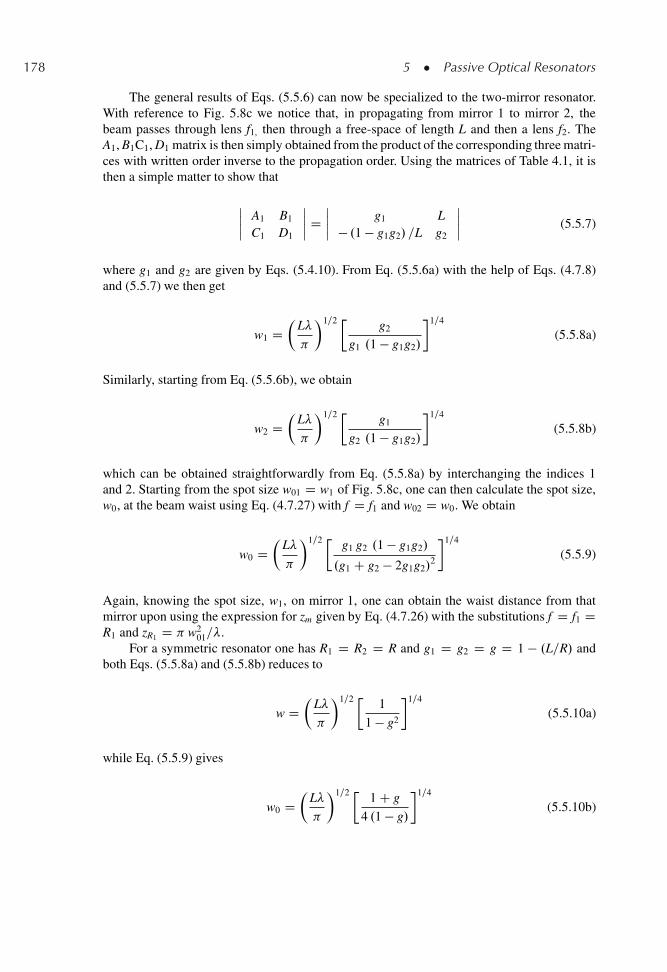
178 5 � Passive Optical Resonators
The general results of Eqs. (5.5.6) can now be specialized to the two-mirror resonator.With reference to Fig. 5.8c we notice that, in propagating from mirror 1 to mirror 2, thebeam passes through lens f1, then through a free-space of length L and then a lens f2. TheA1, B1C1, D1 matrix is then simply obtained from the product of the corresponding three matri-ces with written order inverse to the propagation order. Using the matrices of Table 4.1, it isthen a simple matter to show that
ˇˇ A1 B1
C1 D1
ˇˇ D
ˇˇ g1 L
� .1 � g1g2/ =L g2
ˇˇ (5.5.7)
where g1 and g2 are given by Eqs. (5.4.10). From Eq. (5.5.6a) with the help of Eqs. (4.7.8)and (5.5.7) we then get
w1 D�
L�
�1=2 � g2
g1 .1 � g1g2/
�1=4
(5.5.8a)
Similarly, starting from Eq. (5.5.6b), we obtain
w2 D�
L�
�1=2 � g1
g2 .1 � g1g2/
�1=4
(5.5.8b)
which can be obtained straightforwardly from Eq. (5.5.8a) by interchanging the indices 1and 2. Starting from the spot size w01 D w1 of Fig. 5.8c, one can then calculate the spot size,w0, at the beam waist using Eq. (4.7.27) with f D f1 and w02 D w0. We obtain
w0 D�
L�
�1=2 � g1 g2 .1 � g1g2/
.g1 C g2 � 2g1g2/2
�1=4
(5.5.9)
Again, knowing the spot size, w1, on mirror 1, one can obtain the waist distance from thatmirror upon using the expression for zm given by Eq. (4.7.26) with the substitutions f D f1 DR1 and zR1 D w2
01=�.For a symmetric resonator one has R1 D R2 D R and g1 D g2 D g D 1 � .L=R/ and
both Eqs. (5.5.8a) and (5.5.8b) reduces to
w D�
L�
�1=2 � 1
1 � g2
�1=4
(5.5.10a)
while Eq. (5.5.9) gives
w0 D�
L�
�1=2 � 1 C g
4 .1 � g/
�1=4
(5.5.10b)
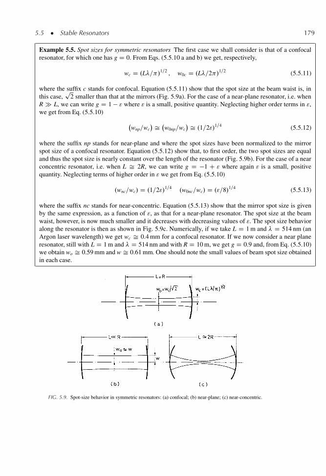
5.5 � Stable Resonators 179
Example 5.5. Spot sizes for symmetric resonators The first case we shall consider is that of a confocalresonator, for which one has g D 0. From Eqs. (5.5.10 a and b) we get, respectively,
wc D .L�= /1=2 , w0c D .L�=2 /1=2 (5.5.11)
where the suffix c stands for confocal. Equation (5.5.11) show that the spot size at the beam waist is, inthis case,
p2 smaller than that at the mirrors (Fig. 5.9a). For the case of a near-plane resonator, i.e. when
R � L, we can write g D 1 � " where " is a small, positive quantity. Neglecting higher order terms in ",we get from Eq. (5.5.10)
wnp=wc
� Š w0np=wc
� Š .1=2"/1=4 (5.5.12)
where the suffix np stands for near-plane and where the spot sizes have been normalized to the mirrorspot size of a confocal resonator. Equation (5.5.12) show that, to first order, the two spot sizes are equaland thus the spot size is nearly constant over the length of the resonator (Fig. 5.9b). For the case of a nearconcentric resonator, i.e. when L Š 2R, we can write g D �1 C " where again " is a small, positivequantity. Neglecting terms of higher order in " we get from Eq. (5.5.10)
.wnc=wc/ D .1=2"/1=4 .w0nc=wc/ D ."=8/1=4 (5.5.13)
where the suffix nc stands for near-concentric. Equation (5.5.13) show that the mirror spot size is givenby the same expression, as a function of ", as that for a near-plane resonator. The spot size at the beamwaist, however, is now much smaller and it decreases with decreasing values of ". The spot size behavioralong the resonator is then as shown in Fig. 5.9c. Numerically, if we take L D 1 m and � D 514 nm (anArgon laser wavelength) we get wc Š 0.4 mm for a confocal resonator. If we now consider a near planeresonator, still with L D 1 m and � D 514 nm and with R D 10 m, we get g D 0.9 and, from Eq. (5.5.10)we obtain wo Š 0.59 mm and w Š 0.61 mm. One should note the small values of beam spot size obtainedin each case.
FIG. 5.9. Spot-size behavior in symmetric resonators: (a) confocal; (b) near-plane; (c) near-concentric.
180 5 � Passive Optical Resonators
5.5.1.2. Eigenvalues
A comparison of Eqs. (4.7.29) with (4.7.30) shows that, if the ABCD matrix correspondsto the cavity round-trip matrix and if q D q1, the field amplitude u.x, y, 2L/ after one roundtrip is equal to the initial field u.x1 D x, y1 D y, z1 D 0/ except for the amplitude factor1= ŒA C .B=q/�1ClCm. According to Eq. (5.2.2) it then follows that
Q�lm D 1
ŒA C .B=q/�1ClCm(5.5.14)
From Eq. (5.5.3) we see that, since A D D, one has
q D jp�B=C (5.5.15)
If we now write
� D A C .B=q/ (5.5.16)
from Eq. (5.5.16), with the help of Eq. (5.5.15), we get j� j2 D A2 � BC D AD � BC D 1.From Eq. (5.5.14) it then follows that the magnitude of Q�lm is also unity and, according toEq. (5.2.6), the diffraction loss, �lm, vanishes. This result is actually to be expected from ouranalysis since we stipulated at the outset that there were no limiting aperture (Fig. 5.8d) andconsidered, in particular, a two-mirror resonator with infinite mirror size (Fig. 5.8c).
To obtain an expression for the phase of the eigenvalue, Q�lm, we write
� D exp �j� (5.5.17)
From Eqs. (5.5.17) and (5.5.16), with the help of Eqs. (5.5.15) and (5.5.5) we get
cos� D A D 2A1D1 � 1 (5.5.18a)
sin � D Bp�C=B D 2B1D1
p�A1C1=B1D1 (5.5.18b)
From Eq. (5.5.18b) we see that 0 < � < for B1D1 > 0 and � < � < 0 for B1D1 < 0.From Eq. (5.5.18a) we get cos2.�=2/ D .1 C cos�/=2 D A1D1 and hence
� D 2 cos�1 ˙p
A1D1 (5.5.19)
where the positive or negative signs hold depending on weather B1D1 is positive or negative.From Eqs. (5.5.14), (5.5.16), and (5.5.17) we obtain Q�lm D exp j.1 C l C m/φ D exp j�lm
where �lm D .1 C l C m/�. From Eqs. (5.5.19) and (5.2.7) we then obtain
�lmn D c
2L
�n C .1 C l C m/
cos�1 ˙
pA1D1
�(5.5.20)
the C or � signs again depending on whether B1D1 is positive or negative.
5.5 � Stable Resonators 181
For the particular case of a two-mirror resonator, the matrix elements A1 and D1 areobtained from Eq. (5.5.7). Equation (5.5.20) then transforms to
�lmn D c
2L
�n C 1 C l C m
cos�1 ˙ p
g1g2
�(5.5.21)
and, according to Eq. (5.5.7), the C or � sign is chosen according to whether g2 (and henceg1) is positive or negative.
Example 5.6. Frequency spectrum of a confocal resonator For a confocal resonator one has g1 D g2 D 0and from Eq. (5.5.21) we get
�lmn D c
4LŒ2n C .1 C l C m/� (5.5.22)
The corresponding frequency spectrum is shown in Fig. 5.10a. One can observe that modes having thesame value of 2n C l C m have the same resonance frequency although they correspond to different spa-tial configurations. These modes are said to be frequency-degenerate. It is also seen that, instead of thesimple expression given by Eq. (5.1.2) for a plane parallel resonator, the frequency spacing betweenconsecutive modes is now c=4L. The two consecutive modes, however, need to have different .l, m/values and c=4L is seen to correspond to the frequency difference between two consecutive transversemodes [e.g. .n, 0, 0/ ! .n, 0, 1/]. On the other hand, the frequency spacing between two modes with thesame .l, m/ values (e.g. TEM00) and with n differing by 1 (i.e. the frequency spacing between adjacentlongitudinal modes) is still c=2L, the same as for the plane parallel resonator.�
Example 5.7. Frequency spectrum of a near-planar and symmetric resonator In this case one has g1 Dg2 D g D 1 � .L=R/, with L=R � 1. Thus g is positive and slightly less than unity. Accordingly one hascos�1 g D cos�1Œ1 � .L=R/� Š .2L=R/1=2 and Eq. (5.5.21) becomes
�lmn D c
2L
"n C .1 C l C m/
�2L
R
�1=2#
(5.5.23)
The corresponding frequency spectrum is shown in Fig. 5.10b. One can see that the frequency spac-ing between consecutive longitudinal modes is again c=2L, while the frequency difference between twoconsecutive transverse modes is .c=2L/ .2L= 2R/1=2.
* The usage of the terms “longitudinal mode” and “transverse mode” in the laser literature has sometimes beenrather confusing, and can convey the (mistaken) impression that there are two distinct types of modes, viz.,longitudinal modes (sometimes called axial modes) and transverse modes. In fact any mode is specified by threenumbers, e.g., n, m, l of (5.5.24). The electric and magnetic fields of the modes are nearly perpendicular to theresonator axis. The variation of these fields in a transverse direction is specified by l, m while field variation in alongitudinal (i.e., axial) direction is specified by n. When one refers, rather loosely, to a (given) transverse mode,it means that one is considering a mode with given values for the transverse indices .l, m/, regardless of the valueof n. Accordingly a single transverse mode means a mode with a single value of the transverse indexes .l, m/. Asimilar interpretation can be applied to the “longitudinal modes”. Thus two consecutive longitudinal modes meantwo modes with consecutive values of the longitudinal index n [i.e., n and .n C 1/ or .n � 1/.
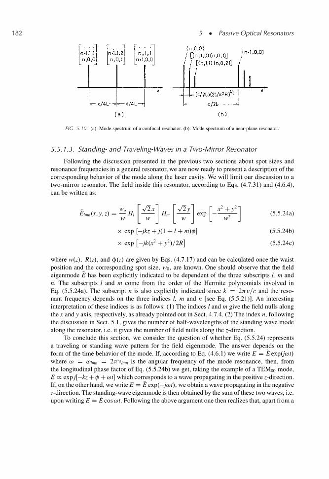
182 5 � Passive Optical Resonators
FIG. 5.10. (a): Mode spectrum of a confocal resonator. (b): Mode spectrum of a near-plane resonator.
5.5.1.3. Standing- and Traveling-Waves in a Two-Mirror Resonator
Following the discussion presented in the previous two sections about spot sizes andresonance frequencies in a general resonator, we are now ready to present a description of thecorresponding behavior of the mode along the laser cavity. We will limit our discussion to atwo-mirror resonator. The field inside this resonator, according to Eqs. (4.7.31) and (4.6.4),can be written as:
QElmn.x, y, z/ D wo
wHl
"p2 x
w
#Hm
"p2 y
w
#exp
��x2 C y2
w2
�(5.5.24a)
� exp Œ�jkz C j.1 C l C m/�� (5.5.24b)
� exp��jk.x2 C y2/=2R
(5.5.24c)
where w.z/, R.z/, and φ.z/ are given by Eqs. (4.7.17) and can be calculated once the waistposition and the corresponding spot size, w0, are known. One should observe that the fieldeigenmode QE has been explicitly indicated to be dependent of the three subscripts l, m andn. The subscripts l and m come from the order of the Hermite polynomials involved inEq. (5.5.24a). The subscript n is also explicitly indicated since k D 2 �=c and the reso-nant frequency depends on the three indices l, m and n [see Eq. (5.5.21)]. An interestinginterpretation of these indices is as follows: (1) The indices l and m give the field nulls alongthe x and y axis, respectively, as already pointed out in Sect. 4.7.4. (2) The index n, followingthe discussion in Sect. 5.1, gives the number of half-wavelengths of the standing wave modealong the resonator, i.e. it gives the number of field nulls along the z-direction.
To conclude this section, we consider the question of whether Eq. (5.5.24) representsa traveling or standing wave pattern for the field eigenmode. The answer depends on theform of the time behavior of the mode. If, according to Eq. (4.6.1) we write E D QE exp.j!t/where ! D !lmn D 2 �lmn is the angular frequency of the mode resonance, then, fromthe longitudinal phase factor of Eq. (5.5.24b) we get, taking the example of a TEM00 mode,E / exp jŒ�kz C�C!t� which corresponds to a wave propagating in the positive z-direction.If, on the other hand, we write E D QE exp.�j!t/, we obtain a wave propagating in the negativez-direction. The standing-wave eigenmode is then obtained by the sum of these two waves, i.e.upon writing E D QE cos!t. Following the above argument one then realizes that, apart from a
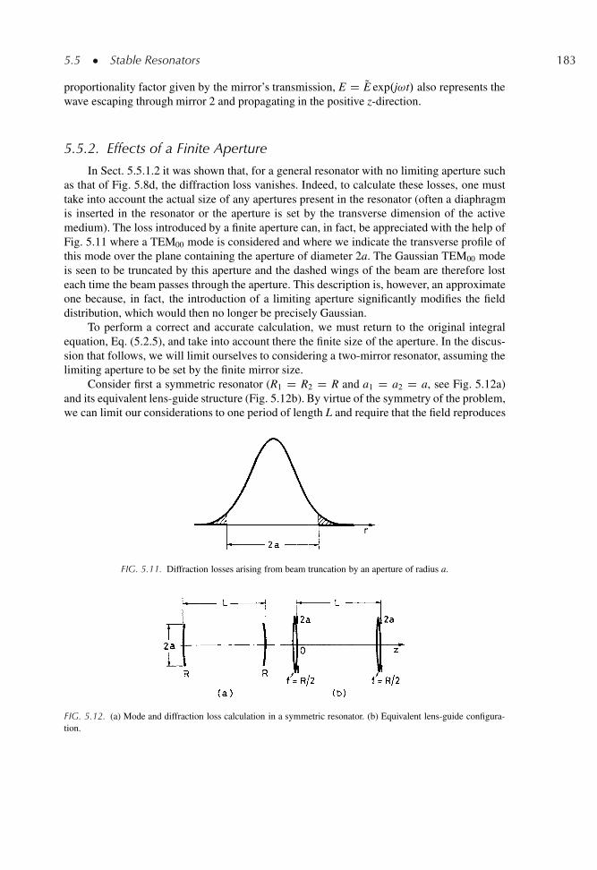
5.5 � Stable Resonators 183
proportionality factor given by the mirror’s transmission, E D QE exp.j!t/ also represents thewave escaping through mirror 2 and propagating in the positive z-direction.
5.5.2. Effects of a Finite Aperture
In Sect. 5.5.1.2 it was shown that, for a general resonator with no limiting aperture suchas that of Fig. 5.8d, the diffraction loss vanishes. Indeed, to calculate these losses, one musttake into account the actual size of any apertures present in the resonator (often a diaphragmis inserted in the resonator or the aperture is set by the transverse dimension of the activemedium). The loss introduced by a finite aperture can, in fact, be appreciated with the help ofFig. 5.11 where a TEM00 mode is considered and where we indicate the transverse profile ofthis mode over the plane containing the aperture of diameter 2a. The Gaussian TEM00 modeis seen to be truncated by this aperture and the dashed wings of the beam are therefore losteach time the beam passes through the aperture. This description is, however, an approximateone because, in fact, the introduction of a limiting aperture significantly modifies the fielddistribution, which would then no longer be precisely Gaussian.
To perform a correct and accurate calculation, we must return to the original integralequation, Eq. (5.2.5), and take into account there the finite size of the aperture. In the discus-sion that follows, we will limit ourselves to considering a two-mirror resonator, assuming thelimiting aperture to be set by the finite mirror size.
Consider first a symmetric resonator (R1 D R2 D R and a1 D a2 D a, see Fig. 5.12a)and its equivalent lens-guide structure (Fig. 5.12b). By virtue of the symmetry of the problem,we can limit our considerations to one period of length L and require that the field reproduces
FIG. 5.11. Diffraction losses arising from beam truncation by an aperture of radius a.
FIG. 5.12. (a) Mode and diffraction loss calculation in a symmetric resonator. (b) Equivalent lens-guide configura-tion.
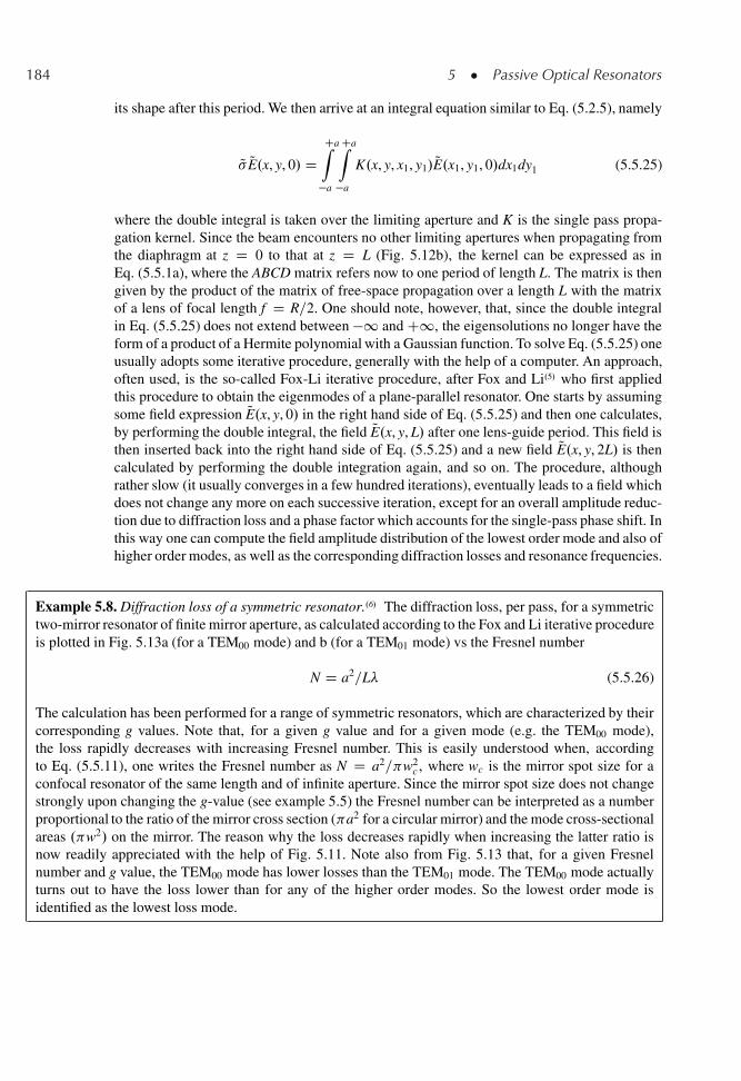
184 5 � Passive Optical Resonators
its shape after this period. We then arrive at an integral equation similar to Eq. (5.2.5), namely
Q� QE.x, y, 0/ DCaZ
�a
CaZ�a
K.x, y, x1, y1/ QE.x1, y1, 0/dx1dy1 (5.5.25)
where the double integral is taken over the limiting aperture and K is the single pass propa-gation kernel. Since the beam encounters no other limiting apertures when propagating fromthe diaphragm at z D 0 to that at z D L (Fig. 5.12b), the kernel can be expressed as inEq. (5.5.1a), where the ABCD matrix refers now to one period of length L. The matrix is thengiven by the product of the matrix of free-space propagation over a length L with the matrixof a lens of focal length f D R=2. One should note, however, that, since the double integralin Eq. (5.5.25) does not extend between �1 and C1, the eigensolutions no longer have theform of a product of a Hermite polynomial with a Gaussian function. To solve Eq. (5.5.25) oneusually adopts some iterative procedure, generally with the help of a computer. An approach,often used, is the so-called Fox-Li iterative procedure, after Fox and Li.5/ who first appliedthis procedure to obtain the eigenmodes of a plane-parallel resonator. One starts by assumingsome field expression QE.x, y, 0/ in the right hand side of Eq. (5.5.25) and then one calculates,by performing the double integral, the field QE.x, y, L/ after one lens-guide period. This field isthen inserted back into the right hand side of Eq. (5.5.25) and a new field QE.x, y, 2L/ is thencalculated by performing the double integration again, and so on. The procedure, althoughrather slow (it usually converges in a few hundred iterations), eventually leads to a field whichdoes not change any more on each successive iteration, except for an overall amplitude reduc-tion due to diffraction loss and a phase factor which accounts for the single-pass phase shift. Inthis way one can compute the field amplitude distribution of the lowest order mode and also ofhigher order modes, as well as the corresponding diffraction losses and resonance frequencies.
Example 5.8. Diffraction loss of a symmetric resonator..6/ The diffraction loss, per pass, for a symmetrictwo-mirror resonator of finite mirror aperture, as calculated according to the Fox and Li iterative procedureis plotted in Fig. 5.13a (for a TEM00 mode) and b (for a TEM01 mode) vs the Fresnel number
N D a2=L� (5.5.26)
The calculation has been performed for a range of symmetric resonators, which are characterized by theircorresponding g values. Note that, for a given g value and for a given mode (e.g. the TEM00 mode),the loss rapidly decreases with increasing Fresnel number. This is easily understood when, accordingto Eq. (5.5.11), one writes the Fresnel number as N D a2= w2
c , where wc is the mirror spot size for aconfocal resonator of the same length and of infinite aperture. Since the mirror spot size does not changestrongly upon changing the g-value (see example 5.5) the Fresnel number can be interpreted as a numberproportional to the ratio of the mirror cross section ( a2 for a circular mirror) and the mode cross-sectionalareas . w2/ on the mirror. The reason why the loss decreases rapidly when increasing the latter ratio isnow readily appreciated with the help of Fig. 5.11. Note also from Fig. 5.13 that, for a given Fresnelnumber and g value, the TEM00 mode has lower losses than the TEM01 mode. The TEM00 mode actuallyturns out to have the loss lower than for any of the higher order modes. So the lowest order mode isidentified as the lowest loss mode.
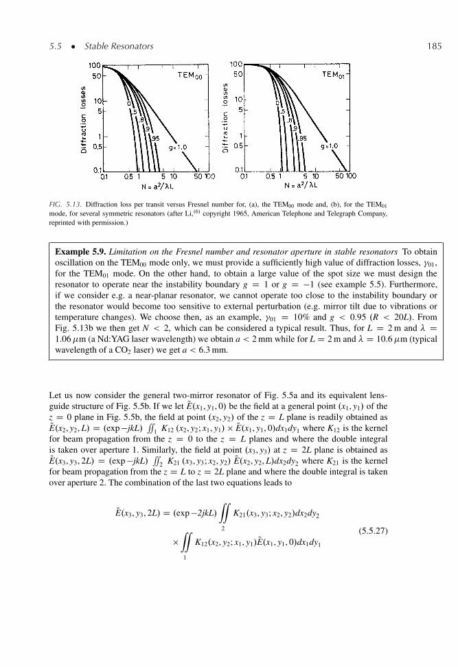
5.5 � Stable Resonators 185
FIG. 5.13. Diffraction loss per transit versus Fresnel number for, (a), the TEM00 mode and, (b), for the TEM01
mode, for several symmetric resonators (after Li,.6/ copyright 1965, American Telephone and Telegraph Company,reprinted with permission.)
Example 5.9. Limitation on the Fresnel number and resonator aperture in stable resonators To obtainoscillation on the TEM00 mode only, we must provide a sufficiently high value of diffraction losses, �01,for the TEM01 mode. On the other hand, to obtain a large value of the spot size we must design theresonator to operate near the instability boundary g D 1 or g D �1 (see example 5.5). Furthermore,if we consider e.g. a near-planar resonator, we cannot operate too close to the instability boundary orthe resonator would become too sensitive to external perturbation (e.g. mirror tilt due to vibrations ortemperature changes). We choose then, as an example, �01 D 10% and g < 0.95 .R < 20L/. FromFig. 5.13b we then get N < 2, which can be considered a typical result. Thus, for L D 2 m and � D1.06�m (a Nd:YAG laser wavelength) we obtain a < 2 mm while for L D 2 m and � D 10.6�m (typicalwavelength of a CO2 laser) we get a < 6.3 mm.
Let us now consider the general two-mirror resonator of Fig. 5.5a and its equivalent lens-guide structure of Fig. 5.5b. If we let QE.x1, y1, 0/ be the field at a general point .x1, y1/ of thez D 0 plane in Fig. 5.5b, the field at point .x2, y2/ of the z D L plane is readily obtained asQE.x2, y2, L/ D .exp �jkL/
’1 K12 .x2, y2; x1, y1/ � QE.x1, y1, 0/dx1dy1 where K12 is the kernel
for beam propagation from the z D 0 to the z D L planes and where the double integralis taken over aperture 1. Similarly, the field at point .x3, y3/ at z D 2L plane is obtained asQE.x3, y3, 2L/ D .exp �jkL/
’2 K21 .x3, y3; x2, y2/ QE.x2, y2, L/dx2dy2 where K21 is the kernel
for beam propagation from the z D L to z D 2L plane and where the double integral is takenover aperture 2. The combination of the last two equations leads to
QE.x3, y3, 2L/ D .exp �2jkL/“2
K21.x3, y3; x2, y2/dx2dy2
�“1
K12.x2, y2; x1, y1/ QE.x1, y1, 0/dx1dy1
(5.5.27)
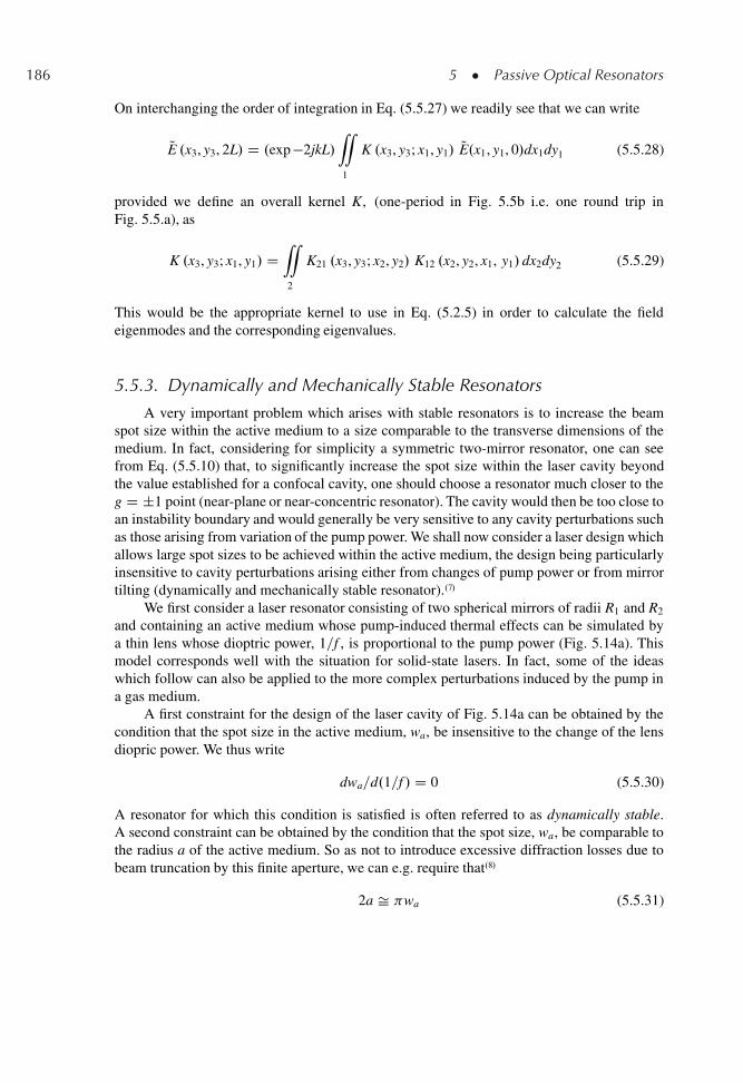
186 5 � Passive Optical Resonators
On interchanging the order of integration in Eq. (5.5.27) we readily see that we can write
QE .x3, y3, 2L/ D .exp �2jkL/“1
K .x3, y3; x1, y1/ QE.x1, y1, 0/dx1dy1 (5.5.28)
provided we define an overall kernel K, (one-period in Fig. 5.5b i.e. one round trip inFig. 5.5.a), as
K .x3, y3; x1, y1/ D“2
K21 .x3, y3; x2, y2/ K12 .x2, y2, x1, y1/ dx2dy2 (5.5.29)
This would be the appropriate kernel to use in Eq. (5.2.5) in order to calculate the fieldeigenmodes and the corresponding eigenvalues.
5.5.3. Dynamically and Mechanically Stable Resonators
A very important problem which arises with stable resonators is to increase the beamspot size within the active medium to a size comparable to the transverse dimensions of themedium. In fact, considering for simplicity a symmetric two-mirror resonator, one can seefrom Eq. (5.5.10) that, to significantly increase the spot size within the laser cavity beyondthe value established for a confocal cavity, one should choose a resonator much closer to theg D ˙1 point (near-plane or near-concentric resonator). The cavity would then be too close toan instability boundary and would generally be very sensitive to any cavity perturbations suchas those arising from variation of the pump power. We shall now consider a laser design whichallows large spot sizes to be achieved within the active medium, the design being particularlyinsensitive to cavity perturbations arising either from changes of pump power or from mirrortilting (dynamically and mechanically stable resonator)..7/
We first consider a laser resonator consisting of two spherical mirrors of radii R1 and R2
and containing an active medium whose pump-induced thermal effects can be simulated bya thin lens whose dioptric power, 1=f , is proportional to the pump power (Fig. 5.14a). Thismodel corresponds well with the situation for solid-state lasers. In fact, some of the ideaswhich follow can also be applied to the more complex perturbations induced by the pump ina gas medium.
A first constraint for the design of the laser cavity of Fig. 5.14a can be obtained by thecondition that the spot size in the active medium, wa, be insensitive to the change of the lensdiopric power. We thus write
dwa=d.1=f / D 0 (5.5.30)
A resonator for which this condition is satisfied is often referred to as dynamically stable.A second constraint can be obtained by the condition that the spot size, wa, be comparable tothe radius a of the active medium. So as not to introduce excessive diffraction losses due tobeam truncation by this finite aperture, we can e.g. require that.8/
2a Š wa (5.5.31)
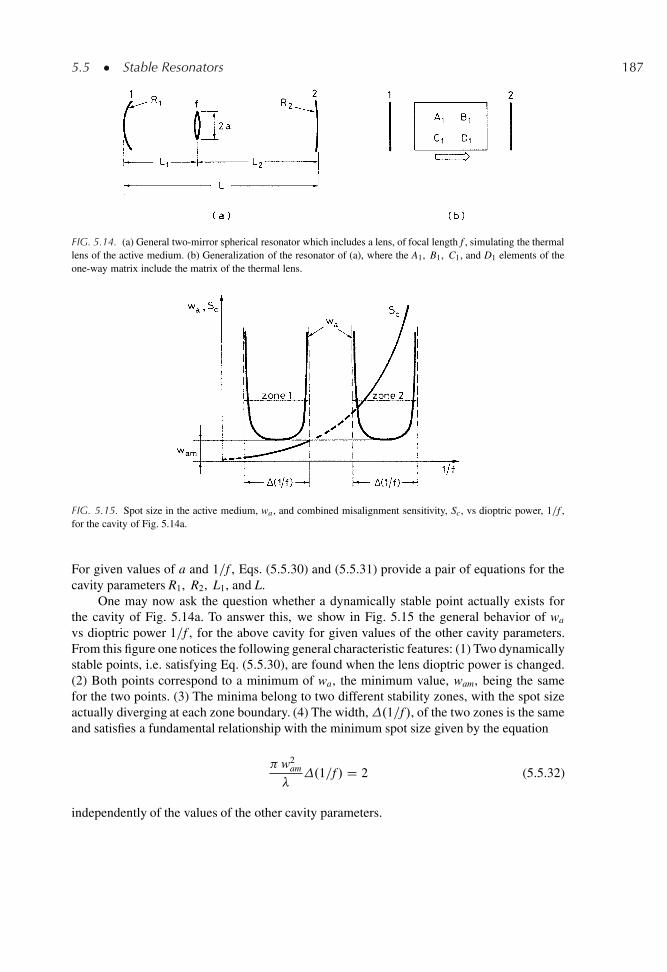
5.5 � Stable Resonators 187
FIG. 5.14. (a) General two-mirror spherical resonator which includes a lens, of focal length f , simulating the thermallens of the active medium. (b) Generalization of the resonator of (a), where the A1, B1, C1, and D1 elements of theone-way matrix include the matrix of the thermal lens.
FIG. 5.15. Spot size in the active medium, wa , and combined misalignment sensitivity, Sc, vs dioptric power, 1=f ,for the cavity of Fig. 5.14a.
For given values of a and 1=f , Eqs. (5.5.30) and (5.5.31) provide a pair of equations for thecavity parameters R1, R2, L1, and L.
One may now ask the question whether a dynamically stable point actually exists forthe cavity of Fig. 5.14a. To answer this, we show in Fig. 5.15 the general behavior of wa
vs dioptric power 1=f , for the above cavity for given values of the other cavity parameters.From this figure one notices the following general characteristic features: (1) Two dynamicallystable points, i.e. satisfying Eq. (5.5.30), are found when the lens dioptric power is changed.(2) Both points correspond to a minimum of wa, the minimum value, wam, being the samefor the two points. (3) The minima belong to two different stability zones, with the spot sizeactually diverging at each zone boundary. (4) The width,.1=f /, of the two zones is the sameand satisfies a fundamental relationship with the minimum spot size given by the equation
w2am
�.1=f / D 2 (5.5.32)
independently of the values of the other cavity parameters.
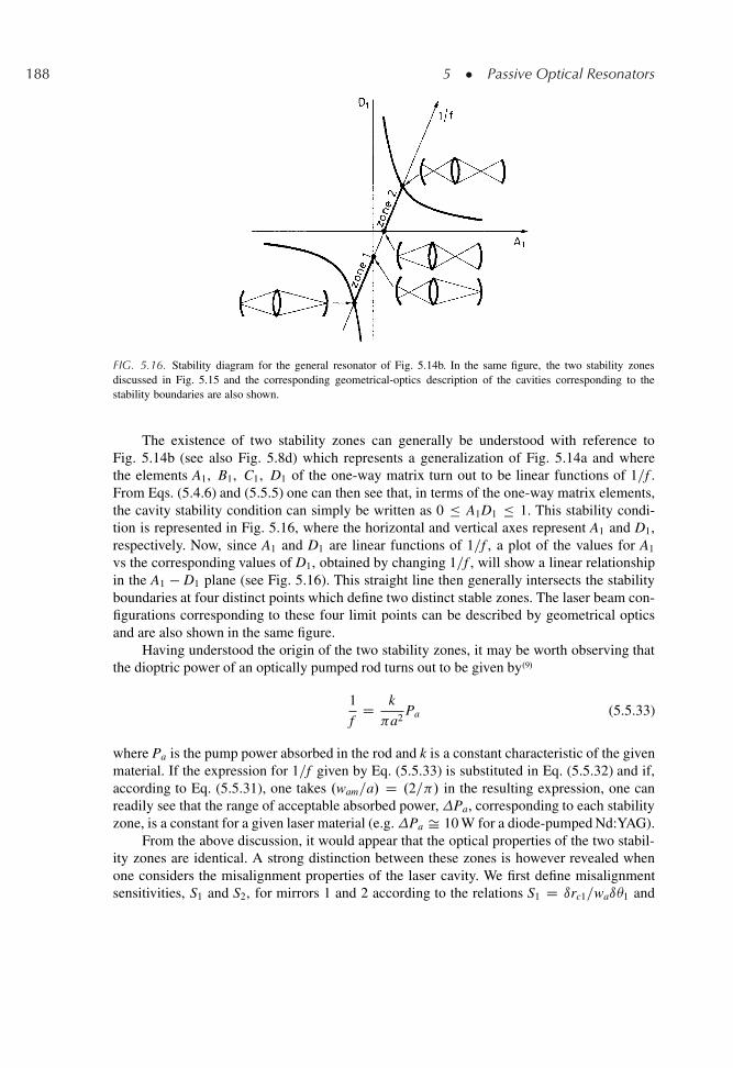
188 5 � Passive Optical Resonators
FIG. 5.16. Stability diagram for the general resonator of Fig. 5.14b. In the same figure, the two stability zonesdiscussed in Fig. 5.15 and the corresponding geometrical-optics description of the cavities corresponding to thestability boundaries are also shown.
The existence of two stability zones can generally be understood with reference toFig. 5.14b (see also Fig. 5.8d) which represents a generalization of Fig. 5.14a and wherethe elements A1, B1, C1, D1 of the one-way matrix turn out to be linear functions of 1=f .From Eqs. (5.4.6) and (5.5.5) one can then see that, in terms of the one-way matrix elements,the cavity stability condition can simply be written as 0 A1D1 1. This stability condi-tion is represented in Fig. 5.16, where the horizontal and vertical axes represent A1 and D1,respectively. Now, since A1 and D1 are linear functions of 1=f , a plot of the values for A1
vs the corresponding values of D1, obtained by changing 1=f , will show a linear relationshipin the A1 � D1 plane (see Fig. 5.16). This straight line then generally intersects the stabilityboundaries at four distinct points which define two distinct stable zones. The laser beam con-figurations corresponding to these four limit points can be described by geometrical opticsand are also shown in the same figure.
Having understood the origin of the two stability zones, it may be worth observing thatthe dioptric power of an optically pumped rod turns out to be given by.9/
1
fD k
a2Pa (5.5.33)
where Pa is the pump power absorbed in the rod and k is a constant characteristic of the givenmaterial. If the expression for 1=f given by Eq. (5.5.33) is substituted in Eq. (5.5.32) and if,according to Eq. (5.5.31), one takes .wam=a/ D .2= / in the resulting expression, one canreadily see that the range of acceptable absorbed power,Pa, corresponding to each stabilityzone, is a constant for a given laser material (e.g.Pa Š 10 W for a diode-pumped Nd:YAG).
From the above discussion, it would appear that the optical properties of the two stabil-ity zones are identical. A strong distinction between these zones is however revealed whenone considers the misalignment properties of the laser cavity. We first define misalignmentsensitivities, S1 and S2, for mirrors 1 and 2 according to the relations S1 D ırc1=waı1 and
5.6 � Unstable Resonators 189
S2 D ırc2=waı2, where, e.g. for mirror 1, ırc1 is the displacement of the beam center inthe laser rod arising from a tilt ı1 of mirror 1, and similarly for mirror 2. One can now
define a combined misalignment sensitivity of the two mirrors as Sc D �S2
1 C S22
1=2. A plot
of this combined sensitivity vs lens dioptric power is also shown in Fig. 5.15. One can thensee that one of the two zones, henceforth referred to as zone 1, is much less sensitive to mir-ror misalignment than the other, henceforth referred to as zone 2. The reason for the reducedsensitivity to misalignment for zone 1 can be understood by noting that the spot sizes at themirrors are much smaller in zone 1 than in zone 2. Indeed, according to geometrical optics,one of the two stability boundaries of zone 1 corresponds to the beam being focused on bothmirrors (see Fig. 5.16). Thus, when close to this boundary, the mirror spot size, wm, is verysmall and the beam divergence, � d D �= wm, very large. Consequently, the mirror tilt,needed to produce a beam axis rotation comparable to the beam divergence, must also be large.
As a conclusion we can say that a dynamically and mechanically stable resonator canbe designed for a general laser cavity describable as in Fig. 5.14b and comprising a variableelement such as the thermally induced lens in the laser rod. The resonator should be chosen tobelong to the more stable zone, zone 1, and must satisfy conditions Eqs. (5.5.30) and (5.5.31).In practice, instead of satisfying Eq. (5.5.30), the resonator can be designed to correspond tothe center of zone 1. So, if the distance L1, shown in Fig. 5.14a, is assumed to be the variableparameter, its value can be taken as the mean of its limiting values, L0
1 and L001 , in zone 1.
From the geometrical optics description shown in Fig. 5.16, one then finds that L01 and L00
1
must satisfy the conditions L0�11 C L�1
2 D f �1 andL00
1 � R1��1 C L�1
2 D f �1, respectively,where L2 is also shown in Fig. 5.14a. Once designed for a given focal length, f , and hence agiven absorbed power, Pa, the resonator can then work for a range of absorbed pump power,Pa, which is the same for a given active medium, independently of the cavity parameters.
5.6. UNSTABLE RESONATORS.10/
The stability condition for a generalized spherical resonator was discussed in Sect. 5.4and the unstable regions were shown to correspond to the unshaded regions of the g1 � g2
plane in Fig. 5.7. Unstable resonators can be separated into two classes: (1) positive branchresonators, which correspond to the case g1g2 > 1, and (2) negative branch resonators, whichcorrespond to the case g1g2 < 0.
Before going on to a quantitative discussion of unstable resonators, it is worth pointingout here the reasons why these resonators are of interest in the laser field. First we note that,according to the results obtained in example 5.5, for a stable resonator corresponding to apoint in the g1 � g2 plane that is not close to an instability boundary, the spot size w istypically of the order of that given for the case of a confocal resonator and, for a wavelengthof �1�m, is usually smaller than 1 mm. We also note that, according to the discussion inexample 5.9, a resonator aperture with radius a < 2 mm needs to be inserted in the laserresonator if oscillation is to be limited to the TEM00 mode. When oscillation is confined to aTEM00 mode of such a small cross section, the power (or energy) available in the output beamis necessarily limited. For unstable resonators, on the contrary, the field does not tend to beconfined to the axis (see, for example, Fig. 5.3), and a large mode volume in a single transverse
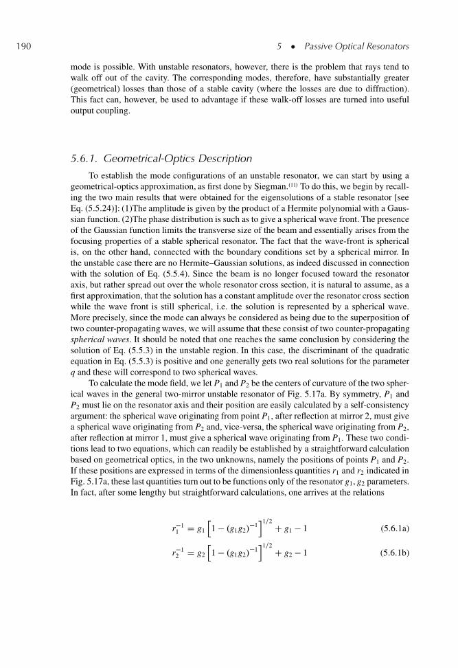
190 5 � Passive Optical Resonators
mode is possible. With unstable resonators, however, there is the problem that rays tend towalk off out of the cavity. The corresponding modes, therefore, have substantially greater(geometrical) losses than those of a stable cavity (where the losses are due to diffraction).This fact can, however, be used to advantage if these walk-off losses are turned into usefuloutput coupling.
5.6.1. Geometrical-Optics Description
To establish the mode configurations of an unstable resonator, we can start by using ageometrical-optics approximation, as first done by Siegman..11/ To do this, we begin by recall-ing the two main results that were obtained for the eigensolutions of a stable resonator [seeEq. (5.5.24)]: (1)The amplitude is given by the product of a Hermite polynomial with a Gaus-sian function. (2)The phase distribution is such as to give a spherical wave front. The presenceof the Gaussian function limits the transverse size of the beam and essentially arises from thefocusing properties of a stable spherical resonator. The fact that the wave-front is sphericalis, on the other hand, connected with the boundary conditions set by a spherical mirror. Inthe unstable case there are no Hermite–Gaussian solutions, as indeed discussed in connectionwith the solution of Eq. (5.5.4). Since the beam is no longer focused toward the resonatoraxis, but rather spread out over the whole resonator cross section, it is natural to assume, as afirst approximation, that the solution has a constant amplitude over the resonator cross sectionwhile the wave front is still spherical, i.e. the solution is represented by a spherical wave.More precisely, since the mode can always be considered as being due to the superposition oftwo counter-propagating waves, we will assume that these consist of two counter-propagatingspherical waves. It should be noted that one reaches the same conclusion by considering thesolution of Eq. (5.5.3) in the unstable region. In this case, the discriminant of the quadraticequation in Eq. (5.5.3) is positive and one generally gets two real solutions for the parameterq and these will correspond to two spherical waves.
To calculate the mode field, we let P1 and P2 be the centers of curvature of the two spher-ical waves in the general two-mirror unstable resonator of Fig. 5.17a. By symmetry, P1 andP2 must lie on the resonator axis and their position are easily calculated by a self-consistencyargument: the spherical wave originating from point P1, after reflection at mirror 2, must givea spherical wave originating from P2 and, vice-versa, the spherical wave originating from P2,after reflection at mirror 1, must give a spherical wave originating from P1. These two condi-tions lead to two equations, which can readily be established by a straightforward calculationbased on geometrical optics, in the two unknowns, namely the positions of points P1 and P2.If these positions are expressed in terms of the dimensionless quantities r1 and r2 indicated inFig. 5.17a, these last quantities turn out to be functions only of the resonator g1, g2 parameters.In fact, after some lengthy but straightforward calculations, one arrives at the relations
r�11 D g1
h1 � .g1g2/
�1i1=2 C g1 � 1 (5.6.1a)
r�12 D g2
h1 � .g1g2/
�1i1=2 C g2 � 1 (5.6.1b)
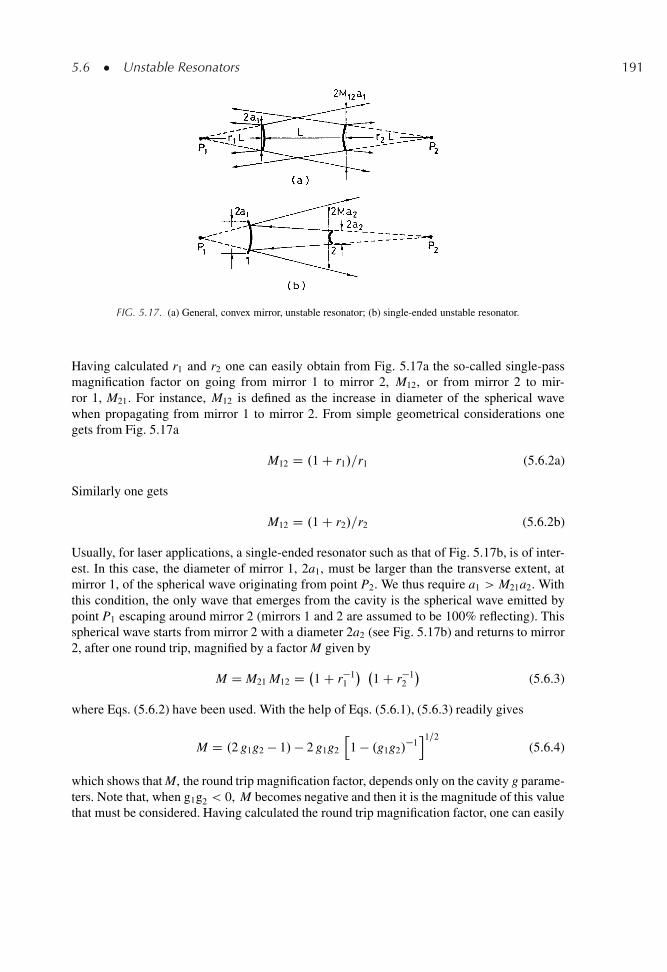
5.6 � Unstable Resonators 191
FIG. 5.17. (a) General, convex mirror, unstable resonator; (b) single-ended unstable resonator.
Having calculated r1 and r2 one can easily obtain from Fig. 5.17a the so-called single-passmagnification factor on going from mirror 1 to mirror 2, M12, or from mirror 2 to mir-ror 1, M21. For instance, M12 is defined as the increase in diameter of the spherical wavewhen propagating from mirror 1 to mirror 2. From simple geometrical considerations onegets from Fig. 5.17a
M12 D .1 C r1/=r1 (5.6.2a)
Similarly one gets
M12 D .1 C r2/=r2 (5.6.2b)
Usually, for laser applications, a single-ended resonator such as that of Fig. 5.17b, is of inter-est. In this case, the diameter of mirror 1, 2a1, must be larger than the transverse extent, atmirror 1, of the spherical wave originating from point P2. We thus require a1 > M21a2. Withthis condition, the only wave that emerges from the cavity is the spherical wave emitted bypoint P1 escaping around mirror 2 (mirrors 1 and 2 are assumed to be 100% reflecting). Thisspherical wave starts from mirror 2 with a diameter 2a2 (see Fig. 5.17b) and returns to mirror2, after one round trip, magnified by a factor M given by
M D M21 M12 D 1 C r�1
1
� 1 C r�1
2
�(5.6.3)
where Eqs. (5.6.2) have been used. With the help of Eqs. (5.6.1), (5.6.3) readily gives
M D .2 g1g2 � 1/� 2 g1g2
h1 � .g1g2/
�1i1=2
(5.6.4)
which shows that M, the round trip magnification factor, depends only on the cavity g parame-ters. Note that, when g1g2 < 0, M becomes negative and then it is the magnitude of this valuethat must be considered. Having calculated the round trip magnification factor, one can easily
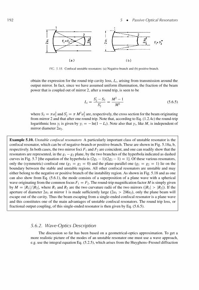
192 5 � Passive Optical Resonators
FIG. 5.18. Confocal unstable resonators: (a) Negative-branch and (b) positive-branch.
obtain the expression for the round trip cavity loss, Li, arising from transmission around theoutput mirror. In fact, since we have assumed uniform illumination, the fraction of the beampower that is coupled out of mirror 2, after a round trip, is seen to be
Li D S02 � S2
S02
D M2 � 1
M2(5.6.5)
where S2 D a22 and S0
2 D M2a22 are, respectively, the cross section for the beam originating
from mirror 2 and that after one round trip. Note that, according to Eq. (1.2.4c) the round-triplogarithmic loss �i is given by �i D � ln.1 � Li/. Note also that �i, like M, is independent ofmirror diameter 2a2.
Example 5.10. Unstable confocal resonators A particularly important class of unstable resonator is theconfocal resonator, which can be of negative-branch or positive-branch. These are shown in Fig. 5.18a, b,respectively. In both cases, the two mirror foci F1 and F2 are coincident, and one can readily show that theresonators are represented, in the g1 � g2 plane, by the two branches of the hyperbola indicated as dashedcurves in Fig. 5.7 [the equation of the hyperbola is .2g1 � 1/.2g2 � 1/ D 1]. Of these various resonators,only the (symmetric) confocal one .g1 D g2 D 0/ and the plane-parallel one .g1 D g2 D 1/ lie on theboundary between the stable and unstable regions. All other confocal resonators are unstable and mayeither belong to the negative or positive branch of the instability region. As shown in Fig. 5.18 and as onecan also show from Eq. (5.6.1), the mode consists of a superposition of a plane wave with a sphericalwave originating from the common focus F1 D F2. The round-trip magnification factor M is simply givenby M D jR1j=jR2j, where R1 and R2 are the two curvature radii of the two mirrors .jR1j > jR2j/. If theaperture of diameter 2a1 at mirror 1 is made sufficiently large .2a1 > 2Ma2/, only the plane beam willescape out of the cavity. Thus the beam escaping from a single-ended confocal resonator is a plane waveand this constitutes one of the main advantages of unstable confocal resonators. The round trip loss, orfractional output coupling, of this single-ended resonator is then given by Eq. (5.6.5).
5.6.2. Wave-Optics Description
The discussion so far has been based on a geometrical-optics approximation. To get amore realistic picture of the modes of an unstable resonator one must use a wave approach,e.g. use the integral equation Eq. (5.2.5), which arises from the Huyghens–Fresnel diffraction
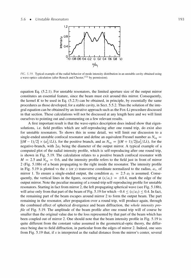
5.6 � Unstable Resonators 193
FIG. 5.19. Typical example of the radial behavior of mode intensity distribution in an unstable cavity obtained usinga wave-optics calculation (after Rensch and Chester,.12/ by permission).
equation Eq. (5.2.1). For unstable resonators, the limited aperture size of the output mirrorconstitutes an essential feature, since the beam must exit around this mirror. Consequently,the kernel K to be used in Eq. (5.2.5) can be obtained, in principle, by essentially the sameprocedures as those developed, for a stable cavity, in Sect. 5.5.2. Thus the solution of the inte-gral equation can be obtained by an iterative approach such as the Fox-Li procedure discussedin that section. These calculations will not be discussed at any length here and we will limitourselves to pointing out and commenting on a few relevant results.
A first important result is that the wave-optics description does indeed show that eigen-solutions, i.e. field profiles which are self-reproducing after one round trip, do exist alsofor unstable resonators. To shows this in some detail, we will limit our discussion to asingle-ended unstable confocal resonator and define an equivalent Fresnel number as Neq DŒ.M � 1/=2� � .a2
2=L�/, for the positive branch, and as Neq D Œ.M C 1/=2�.a22=L�/, for the
negative-branch, with 2a2 being the diameter of the output mirror. A typical example of acomputed plot of the radial intensity profile, which is self-reproducing after one round trip,is shown in Fig. 5.19. The calculation relates to a positive branch confocal resonator withM D 2.5 and Neq D 0.6, and the intensity profile refers to the field just in front of mirror2 (Fig. 5.18b) of a beam propagating to the right inside the resonator. The intensity profilein Fig. 5.19 is plotted vs the x (or y) transverse coordinate normalized to the radius, a1, ofmirror 1. To ensure a single-ended output, the condition a1 D 2.5 a2 is assumed. Conse-quently, the vertical lines in the figure, occurring at .x=a1/ D ˙0.4, mark the edge of theoutput mirror. Note the peculiar meaning of a round-trip self-reproducing profile for unstableresonators. Starting in fact from mirror 2, the left propagating spherical wave (see Fig. 5.18b),will arise only from that part of the beam of Fig. 5.19 for which �0.4 .x=a1/ 0.4. In fact,the remaining part of the beam escapes around mirror 2 to form the output beam. The partremaining in the resonator, after propagation over a round trip, will produce again, throughthe combined effect of spherical divergence and beam diffraction, the whole intensity pro-file of Fig. 5.19. The amplitude of the beam profile after one round trip will of course besmaller than the original value due to the loss represented by that part of the beam which hasbeen coupled out of mirror 2. One should note that the beam intensity profile in Fig. 5.19 isquite different from the constant value assumed in the geometrical-optic theory, the differ-ence being due to field diffraction, in particular from the edges of mirror 2. Indeed, one seesfrom Fig. 5.19 that, if x is interpreted as the radial distance from the mirror’s center, several
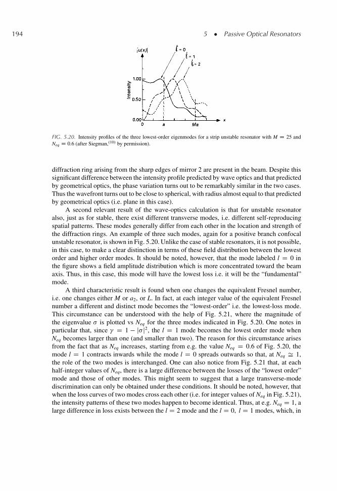
194 5 � Passive Optical Resonators
FIG. 5.20. Intensity profiles of the three lowest-order eigenmodes for a strip unstable resonator with M D 25 andNeq D 0.6 (after Siegman,.10/ by permission).
diffraction ring arising from the sharp edges of mirror 2 are present in the beam. Despite thissignificant difference between the intensity profile predicted by wave optics and that predictedby geometrical optics, the phase variation turns out to be remarkably similar in the two cases.Thus the wavefront turns out to be close to spherical, with radius almost equal to that predictedby geometrical optics (i.e. plane in this case).
A second relevant result of the wave-optics calculation is that for unstable resonatoralso, just as for stable, there exist different transverse modes, i.e. different self-reproducingspatial patterns. These modes generally differ from each other in the location and strength ofthe diffraction rings. An example of three such modes, again for a positive branch confocalunstable resonator, is shown in Fig. 5.20. Unlike the case of stable resonators, it is not possible,in this case, to make a clear distinction in terms of these field distribution between the lowestorder and higher order modes. It should be noted, however, that the mode labeled l D 0 inthe figure shows a field amplitude distribution which is more concentrated toward the beamaxis. Thus, in this case, this mode will have the lowest loss i.e. it will be the “fundamental”mode.
A third characteristic result is found when one changes the equivalent Fresnel number,i.e. one changes either M or a2, or L. In fact, at each integer value of the equivalent Fresnelnumber a different and distinct mode becomes the “lowest-order” i.e. the lowest-loss mode.This circumstance can be understood with the help of Fig. 5.21, where the magnitude ofthe eigenvalue � is plotted vs Neq for the three modes indicated in Fig. 5.20. One notes inparticular that, since � D 1 � j� j2, the l D 1 mode becomes the lowest order mode whenNeq becomes larger than one (and smaller than two). The reason for this circumstance arisesfrom the fact that as Neq increases, starting from e.g. the value Neq D 0.6 of Fig. 5.20, themode l D 1 contracts inwards while the mode l D 0 spreads outwards so that, at Neq Š 1,the role of the two modes is interchanged. One can also notice from Fig. 5.21 that, at eachhalf-integer values of Neq, there is a large difference between the losses of the “lowest order”mode and those of other modes. This might seem to suggest that a large transverse-modediscrimination can only be obtained under these conditions. It should be noted, however, thatwhen the loss curves of two modes cross each other (i.e. for integer values of Neq in Fig. 5.21),the intensity patterns of these two modes happen to become identical. Thus, at e.g. Neq D 1, alarge difference in loss exists between the l D 2 mode and the l D 0, l D 1 modes, which, in
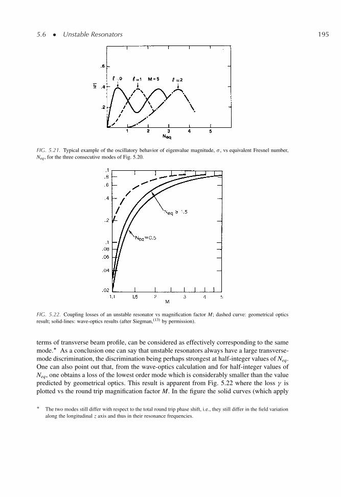
5.6 � Unstable Resonators 195
FIG. 5.21. Typical example of the oscillatory behavior of eigenvalue magnitude, � , vs equivalent Fresnel number,Neq , for the three consecutive modes of Fig. 5.20.
FIG. 5.22. Coupling losses of an unstable resonator vs magnification factor M; dashed curve: geometrical opticsresult; solid-lines: wave-optics results (after Siegman,.13/ by permission).
terms of transverse beam profile, can be considered as effectively corresponding to the samemode.� As a conclusion one can say that unstable resonators always have a large transverse-mode discrimination, the discrimination being perhaps strongest at half-integer values of Neq.One can also point out that, from the wave-optics calculation and for half-integer values ofNeq, one obtains a loss of the lowest order mode which is considerably smaller than the valuepredicted by geometrical optics. This result is apparent from Fig. 5.22 where the loss � isplotted vs the round trip magnification factor M. In the figure the solid curves (which apply
� The two modes still differ with respect to the total round trip phase shift, i.e., they still differ in the field variationalong the longitudinal z axis and thus in their resonance frequencies.
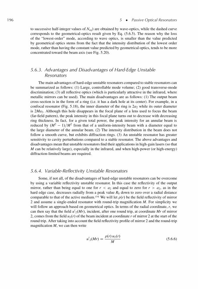
196 5 � Passive Optical Resonators
to successive half-integer values of Neq/ are obtained by wave-optics, while the dashed curvecorresponds to the geometrical-optics result given by Eq. (5.6.5). The reason why the lossof the “lowest-order” mode, according to wave optics, is smaller than the value predictedby geometrical optics stems from the fact that the intensity distribution of the lowest ordermode, rather than having the constant value predicted by geometrical optics, tends to be moreconcentrated toward the beam axis (see Fig. 5.20).
5.6.3. Advantages and Disadvantages of Hard-Edge UnstableResonators
The main advantages of hard-edge unstable resonators compared to stable resonators canbe summarized as follows: (1) Large, controllable mode volume; (2) good transverse-modediscrimination; (3) all reflective optics (which is particularly attractive in the infrared, wheremetallic mirrors can be used). The main disadvantages are as follows: (1) The output beamcross-section is in the form of a ring (i.e. it has a dark hole at its center). For example, in aconfocal resonator (Fig. 5.18), the inner diameter of the ring is 2a2 while its outer diameteris 2Ma2. Although this hole disappears in the focal plane of a lens used to focus the beam(far-field pattern), the peak intensity in this focal plane turns out to decrease with decreasingring thickness. In fact, for a given total power, the peak intensity for an annular beam isreduced by .M2 � 1/=M2 from that of a uniform-intensity beam with a diameter equal tothe large diameter of the annular beam. (2) The intensity distribution in the beam does notfollow a smooth curve, but exhibits diffraction rings. (3) An unstable resonator has greatersensitivity to cavity perturbations compared to a stable resonator. The above advantages anddisadvantages mean that unstable resonators find their applications in high-gain lasers (so thatM can be relatively large), especially in the infrared, and when high-power (or high-energy)diffraction-limited beams are required.
5.6.4. Variable-Reflectivity Unstable Resonators
Some, if not all, of the disadvantages of hard-edge unstable resonators can be overcomeby using a variable reflectivity unstable resonator. In this case the reflectivity of the outputmirror, rather than being equal to one for r < a2 and equal to zero for r > a2, as in thehard edge case, decreases radially from a peak value R0 down to zero over a radial distancecomparable to that of the active medium..14/ We will let �.r/ be the field reflectivity of mirror2 and assume a single-ended resonator with round-trip magnification M. For simplicity wewill follow an approach based on geometrical optics. In terms of the radial coordinate, r, wecan then say that the field u0
2.Mr/, incident, after one round trip, at coordinate Mr of mirror2, comes from the field u2.r/ of the beam incident at coordinate r of mirror 2 at the start of theround trip. After taking into account the field reflectivity profile of mirror 2 and the round-tripmagnification M, we can then write
u02.Mr/ D �.r/ u2.r/
M(5.6.6)
5.6 � Unstable Resonators 197
Note the quantity M appearing at the denominator of the right hand side of Eq. (5.6.6). Thisis a consequence of the fact that, after a magnification by a factor M, the beam area increasesby a factor M2. To conserve the power of the beam, the intensity must therefore decrease by afactor M2 and the field by a factor M. If u2 corresponds to a cavity mode, then it follows thatu0
2.r/ D �u2.r/ where � is now a real quantity, with magnitude smaller than unity, in orderto account for cavity losses. From Eq. (5.6.6) we then get
� u2.Mr/ D �.r/ u2.r/
M(5.6.7)
The eigensolutions u2.r/ D u2l.r/ of Eq. (5.6.7) will give the field distributions inside thecavity, in front of mirror 2, while the eigenvalues of Eq. (5.6.7) will give the round-trip losses,due to the output coupling, according to the familiar relation (see Eq. (5.2.6))
� D 1 � �2 (5.6.8)
The first case that we shall consider is that of a Gaussian reflectivity profile..11,12/ Wetherefore write
� D �0 exp�r2=w2
m
�(5.6.9)
where �0 is the peak field reflectivity and wm sets the transverse scale of the mirror reflectivityprofile. One should note that, according to Eq. (5.6.9), the intensity reflectivity profile, whichis the quantity usually measured experimentally, will be given by
R D R0 exp.�2r2=w2m/ (5.6.10)
where R0 D �20 is the peak reflectivity. With the help of Eq. (5.6.9), the lowest order solution
of Eq. (5.6.7) can be shown, by direct substitution, to be given by
u20.r/ D u20.0/ exp.�r2=w2/ (5.6.11)
where
w2 D .M2 � 1/w2m (5.6.12)
The corresponding eigenvalue � is
� D �0=M (5.6.13)
so that, according to Eq. (5.6.8), the output coupling losses are given by
� D 1 � .R0=M2/ (5.6.14)
The radial intensity distribution for the beam incident on mirror 2 is then given by
Iin.r/ D Iin.0/ exp.�2r2=w2/ (5.6.15)
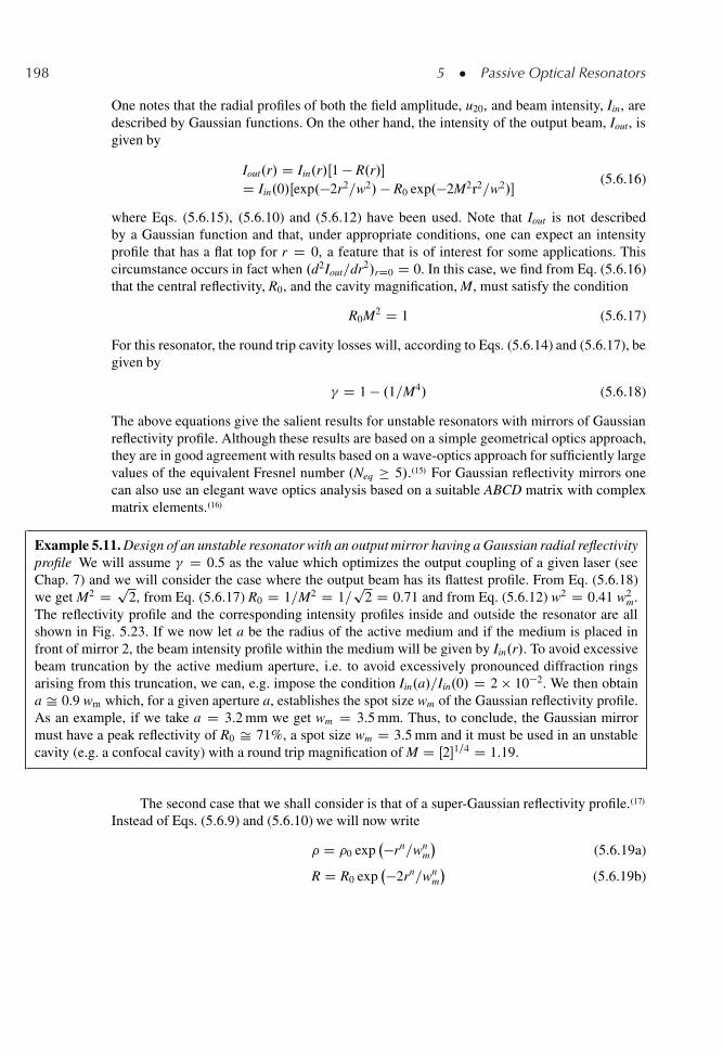
198 5 � Passive Optical Resonators
One notes that the radial profiles of both the field amplitude, u20, and beam intensity, Iin, aredescribed by Gaussian functions. On the other hand, the intensity of the output beam, Iout, isgiven by
Iout.r/ D Iin.r/Œ1 � R.r/�D Iin.0/Œexp.�2r2=w2/ � R0 exp.�2M2r2=w2/�
(5.6.16)
where Eqs. (5.6.15), (5.6.10) and (5.6.12) have been used. Note that Iout is not describedby a Gaussian function and that, under appropriate conditions, one can expect an intensityprofile that has a flat top for r D 0, a feature that is of interest for some applications. Thiscircumstance occurs in fact when .d2Iout=dr2/rD0 D 0. In this case, we find from Eq. (5.6.16)that the central reflectivity, R0, and the cavity magnification, M, must satisfy the condition
R0M2 D 1 (5.6.17)
For this resonator, the round trip cavity losses will, according to Eqs. (5.6.14) and (5.6.17), begiven by
� D 1 � .1=M4/ (5.6.18)
The above equations give the salient results for unstable resonators with mirrors of Gaussianreflectivity profile. Although these results are based on a simple geometrical optics approach,they are in good agreement with results based on a wave-optics approach for sufficiently largevalues of the equivalent Fresnel number .Neq 5/..15/ For Gaussian reflectivity mirrors onecan also use an elegant wave optics analysis based on a suitable ABCD matrix with complexmatrix elements..16/
Example 5.11. Design of an unstable resonator with an output mirror having a Gaussian radial reflectivityprofile We will assume � D 0.5 as the value which optimizes the output coupling of a given laser (seeChap. 7) and we will consider the case where the output beam has its flattest profile. From Eq. (5.6.18)we get M2 D p
2, from Eq. (5.6.17) R0 D 1=M2 D 1=p
2 D 0.71 and from Eq. (5.6.12) w2 D 0.41 w2m.
The reflectivity profile and the corresponding intensity profiles inside and outside the resonator are allshown in Fig. 5.23. If we now let a be the radius of the active medium and if the medium is placed infront of mirror 2, the beam intensity profile within the medium will be given by Iin.r/. To avoid excessivebeam truncation by the active medium aperture, i.e. to avoid excessively pronounced diffraction ringsarising from this truncation, we can, e.g. impose the condition Iin.a/=Iin.0/ D 2 � 10�2. We then obtaina Š 0.9 wm which, for a given aperture a, establishes the spot size wm of the Gaussian reflectivity profile.As an example, if we take a D 3.2 mm we get wm D 3.5 mm. Thus, to conclude, the Gaussian mirrormust have a peak reflectivity of R0 Š 71%, a spot size wm D 3.5 mm and it must be used in an unstablecavity (e.g. a confocal cavity) with a round trip magnification of M D Œ2�1=4 D 1.19.
The second case that we shall consider is that of a super-Gaussian reflectivity profile..17/
Instead of Eqs. (5.6.9) and (5.6.10) we will now write
� D �0 exp�rn=wn
m
�(5.6.19a)
R D R0 exp�2rn=wn
m
�(5.6.19b)
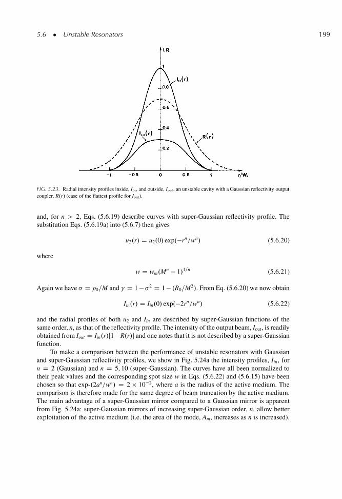
5.6 � Unstable Resonators 199
FIG. 5.23. Radial intensity profiles inside, Iin, and outside, Iout , an unstable cavity with a Gaussian reflectivity outputcoupler, R.r/ (case of the flattest profile for Iout).
and, for n > 2, Eqs. (5.6.19) describe curves with super-Gaussian reflectivity profile. Thesubstitution Eqs. (5.6.19a) into (5.6.7) then gives
u2.r/ D u2.0/ exp.�rn=wn/ (5.6.20)
where
w D wm.Mn � 1/1=n (5.6.21)
Again we have � D �0=M and � D 1 � �2 D 1 � .R0=M2/. From Eq. (5.6.20) we now obtain
Iin.r/ D Iin.0/ exp.�2rn=wn/ (5.6.22)
and the radial profiles of both u2 and Iin are described by super-Gaussian functions of thesame order, n, as that of the reflectivity profile. The intensity of the output beam, Iout, is readilyobtained from Iout D Iin.r/Œ1�R.r/� and one notes that it is not described by a super-Gaussianfunction.
To make a comparison between the performance of unstable resonators with Gaussianand super-Gaussian reflectivity profiles, we show in Fig. 5.24a the intensity profiles, Iin, forn D 2 (Gaussian) and n D 5, 10 (super-Gaussian). The curves have all been normalized totheir peak values and the corresponding spot size w in Eqs. (5.6.22) and (5.6.15) have beenchosen so that exp-.2an=wn/ D 2 � 10�2, where a is the radius of the active medium. Thecomparison is therefore made for the same degree of beam truncation by the active medium.The main advantage of a super-Gaussian mirror compared to a Gaussian mirror is apparentfrom Fig. 5.24a: super-Gaussian mirrors of increasing super-Gaussian order, n, allow betterexploitation of the active medium (i.e. the area of the mode, Am, increases as n is increased).
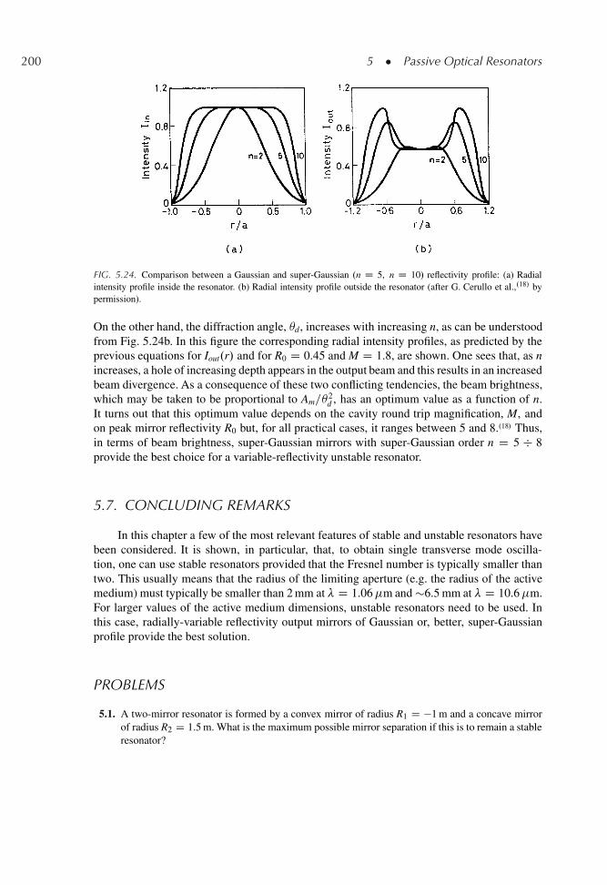
200 5 � Passive Optical Resonators
FIG. 5.24. Comparison between a Gaussian and super-Gaussian .n D 5, n D 10/ reflectivity profile: (a) Radialintensity profile inside the resonator. (b) Radial intensity profile outside the resonator (after G. Cerullo et al.,.18/ bypermission).
On the other hand, the diffraction angle, d, increases with increasing n, as can be understoodfrom Fig. 5.24b. In this figure the corresponding radial intensity profiles, as predicted by theprevious equations for Iout.r/ and for R0 D 0.45 and M D 1.8, are shown. One sees that, as nincreases, a hole of increasing depth appears in the output beam and this results in an increasedbeam divergence. As a consequence of these two conflicting tendencies, the beam brightness,which may be taken to be proportional to Am=
2d , has an optimum value as a function of n.
It turns out that this optimum value depends on the cavity round trip magnification, M, andon peak mirror reflectivity R0 but, for all practical cases, it ranges between 5 and 8..18/ Thus,in terms of beam brightness, super-Gaussian mirrors with super-Gaussian order n D 5 � 8provide the best choice for a variable-reflectivity unstable resonator.
5.7. CONCLUDING REMARKS
In this chapter a few of the most relevant features of stable and unstable resonators havebeen considered. It is shown, in particular, that, to obtain single transverse mode oscilla-tion, one can use stable resonators provided that the Fresnel number is typically smaller thantwo. This usually means that the radius of the limiting aperture (e.g. the radius of the activemedium) must typically be smaller than 2 mm at � D 1.06�m and �6.5 mm at � D 10.6�m.For larger values of the active medium dimensions, unstable resonators need to be used. Inthis case, radially-variable reflectivity output mirrors of Gaussian or, better, super-Gaussianprofile provide the best solution.
PROBLEMS
5.1. A two-mirror resonator is formed by a convex mirror of radius R1 D �1 m and a concave mirrorof radius R2 D 1.5 m. What is the maximum possible mirror separation if this is to remain a stableresonator?
Problems 201
5.2. Consider a confocal resonator of length L D 1 m used for an ArC laser at wavelength � D514.5 nm. Calculate: (a) the spot size at the resonator center and on the mirrors; (b) the frequencydifference between consecutive longitudinal modes; (c) the number of non-degenerate modesfalling within the Doppler-broadened width of the ArC line (��
0 D 3.5 GHz, see Table 2.2)
5.3. Consider a hemiconfocal resonator (plane-spherical resonator with L D R=2) of length L D 2 mused for a CO2 laser at a wavelength of � D 10.6�m. Calculate: (a) the location of the beamwaist; (b) the spot size on each mirror; (c) the frequency difference between two consecutiveTEM00 modes; (d) the number of TEM00 modes falling within the laser linewidth (consider atypical low pressure CO2 laser and thus take � ' 50 MHz).
5.4. Consider a resonator consisting of two concave spherical mirrors both with radius of curvature 4 mand separated by a distance of 1 m. Calculate the spot size of the TEM00 mode at the resonatorcenter and on the mirrors when the laser oscillation is at the ArC laser wavelength � D 514.5 nm.
5.5. How is the spot size modified at each mirror if one of the mirrors of the above problem is replacedby a plane mirror?
5.6. Using Eqs. (4.7.26) and (5.5.8a), show that the beam waist for the two-mirror resonator ofFig. 5.8b occurs at a distance, z1, from mirror 1 given by z1 D .1 � g1/g2L=.g1 C g2 � 2g1g2/.
5.7. One of the mirrors in the resonator of Problem 5.4 is replaced by a concave mirror of 1.5 m radiusof curvature. Using the result of Problem 5.6, calculate: (1) the position of the beam waist; (2) thespot size at the beam waist and on each mirror.
5.8. A resonator consists of two plane mirrors with a positive lens inserted between the two mirrors. Ifthe focal length of the lens is f , and L1 and L2 are the distances of the lens from the two mirrors,calculate: (1) the spot size at the lens position, and the spot sizes at each mirror; (2) the conditionsunder which the cavity is stable.
5.9. A triangular ring cavity is made up of three plane mirrors (Fig. 5.4a) with a positive lens insertedbetween two of the mirrors. If p is the length of the ring perimeter, calculate the position ofminimum spot size, its value, and the spot size at the lens position. Also find the stability conditionfor this cavity.
5.10. A laser operating at � D 630 nm has a power gain of 2 � 10�2 per pass and is provided with asymmetric resonator consisting of two mirrors each of radius R D 10 m and spaced by L D 1 m.Choose an appropriate size of mirror aperture in order to suppress TEM01 mode operation whileallowing TEM00 mode operation.
5.11. On account of its relatively small sensitivity to mirror misalignment (see problem 5.16), a nearlyhemispherical resonator (i.e. a plane-spherical resonator with R D L C and � L) is oftenused for a He-Ne laser at � D 630 nm wavelength. If the cavity length is L D 30 cm, calculate: (1)the radius of curvature of the spherical mirror so that the spot size at this mirror is wm D 0.5 mm;(2) the location in the g1–g2 plane corresponding to this resonator; (3) the spot size at the planemirror.
5.12. Consider the nearly hemispherical He-Ne resonator of the previous problem and assume that theaperturing effect produced by the bore of the capillary containing the He-Ne gas mixture (seeChap. 10) can be simulated by a diaphragm of radius, a, in front of the spherical mirror. If thepower gain per pass of the He-Ne laser is taken to be 2 � 10�2, calculate the diaphragm radiusneeded to suppress the TEM01 mode (Hint: Show that the round-trip loss of this resonator is thesame as the single pass loss of a near concentric symmetric resonator of length Lnc D 2L andR1 D R2 D R. To calculate diffraction loss, then use Fig. 5.13, assuming the loss for a resonator
202 5 � Passive Optical Resonators
of negative g-value to be the same as that of the corresponding resonator with correspondingpositive g-value).
5.13. Consider the A1B1C1D1 matrix of Fig. 5.8d and show that, for a stable cavity, one must have0 < A1D1 < 1 and �1 < B1C1 < 0. From these results, then show that B1D1=A1C1 < 0 so thatq1 in Eq. (5.5.6a) is purely imaginary.
5.14. For a stable two-mirror resonator one can define a misalignment sensitivity, ı, as the transverseshift of the intersection of the optical axis with a given mirror, normalized to the spot size onthat mirror, for a unit angular tilt of one of the two mirrors. In particular, for mirror 1, one candefine two misalignment sensitivity factors ı11 and ı12 as ı11 D .1=w1/.dr1=d1/ and ı12 D.1=w1/.dr1=d2/, where dr1=di .i D 1, 2/ is the transverse change of beam center at mirror 1for unit angular tilt of either mirror 1 or 2. Show that, for a confocal resonator, .ı11/c D 0 and.ı12/c D . ws=�/.
5.15. Using the definitions given in the previous problem, show that, for a near-plane symmetric res-onator, the misalignment sensitivity is such that ı11 D ı12 D ı21 D ı22 D .ı12/c4w3=w2
s , where.ı12/c is the misalignment sensitivity of the confocal resonator, w is the spot size on the mirrorfor the actual resonator and ws is the mirror spot size of a confocal resonator of the same length.According to the above equation which of the two resonators is the less sensitive to mirror tilt?
5.16. Consider a nearly hemispherical resonator (R D LCwith � L) in which mirror 1 is the planemirror. Show that we have in this case ı12 D .ı12/c.w2=ws/ and ı21 D .ı12/c.ws=w2/. Comparingthis resonator with the long radius resonator of the previous problem, for the same value of mirrorspot-size, i.e. w D w2, what conclusion can be drawn with regard to the misalignment sensitivityof a nearly hemispherical resonator compared to that of a nearly flat resonator?
5.17. An unstable resonator consists of a plane mirror (mirror 1) and a convex mirror (mirror 2) of radiusof curvature R2 D 2 m, spaced by a distance L D 50 cm. Calculate: (1) The resonator location inthe g1, g2 plane. (2) The location of points P1 and P2 of Fig. 5.17. (3) The condition under whichthe resonator is single-ended with beam output only occurring around mirror 2. (4) The round-tripmagnification factor and the round trip losses.
5.18. A confocal unstable resonator is to be used for a CO2 laser at a wavelength of � D 10.6�m.The resonator length is chosen to be L D 1 m. Which branch would you choose for this resonatorif the mode volume is to be maximized? Calculate the mirror apertures 2a1 and 2a2 so that: (1)Neq D 7.5, (2) single-ended output is achieved, and (3) a 20% round-trip output coupling isobtained. Then find the radii of the two mirrors R1 and R2.
5.19. Using a geometrical-optics approach (and assuming lowest-order mode oscillation), calculate theround-trip loss of the resonator designed in the above problem. What are the shape and dimensionsof the output beam?
5.20. Consider an unstable resonator consisting of a convex mirror, mirror 1, of radius R1 and a planemirror (mirror 2) spaced by a distance L D 50 cm. Assume that the plane mirror has a super-Gaussian reflectivity profile with a super-Gaussian order n D 6 and peak power reflectivityR0 D 0.5. Assume also that the active medium consists of a cylindrical rod (e.g. a Nd:YAGrod) with radius a Š 3.2 mm, placed just in front of mirror 2. To limit the round-trip losses toan acceptable value, assume also a round trip magnification M D 1.4. Calculate: (1) The spotsize w of the field intensity, Iin, for a 2 � 10�2 intensity truncation by the active medium. (2) Thecorresponding mirror spot size wm. (3) The cavity round trip losses. (4) The radius of curvature ofthe convex mirror.
References 203
References
1. A.E. Siegman, Lasers (University Science Books, Mill Valley, California, 1986) sect. 14.22. M. Born and E. Wolf, Principles of Optics, 6th ed. (Pergamon Press, London 1980) sect. 1.6.53. H. Kogelnik and T. Li, Laser Beams and Resonators, Appl. Opt. 5, 1550 (1966)4. Reference [1], Chap. 195. A.G. Fox and T. Li, Resonant Modes in a Maser Interferometer, Bell. Syst. Tech. J. 40, 453 (1961)6. T. Li, Diffraction Loss and Selection of Modes in Maser Resonators with Circular Mirrors, Bell. Syst.Tech. J.
44, 917 (1965)7. V. Magni, Resonators for Solid-State Lasers with Large-Volume Fundamental Mode and High Alignment
Stability, Appl. Opt., 25, 107–117 (1986). See also erratum Appl. Opt., 25, 2039 (1986)8. Reference [1], p. 6669. W. Koechner, Solid-State Laser Engineering, Vol. 1, Springer Series in Optical Sciences, fourth edition
(Springer, New York, 1996)10. Reference [1], Chap. 2211. A.E. Siegman, Unstable Optical Resonators for Laser Applications, Proc. IEEE 53, 277–287 (1965)12. D.B. Rensch and A.N. Chester, Iterative Diffraction Calculations of Transverse Mode Distributions in Confocal
Unstable Laser Resonators, Appl. Opt. 12, 997 (1973)13. A.E. Siegman, Stabilizing Output with Unstable Resonators, Laser Focus 7, 42 (1971)14. H. Zucker, Optical Resonators with Variable Reflectivity Mirrors, Bell. Syst. Tech. J. 49, 2349 (1970)15. A.N. Chester, Mode Selectivity and Mirror Misalignment Effects in Unstable Laser Resonators, Appl. Opt. 11,
2584 (1972)16. Ref. [1], sect. 23.317. S. De Silvestri, P. Laporta, V. Magni and O. Svelto, Solid-State Unstable Resonators with Tapered Reflectivity
Mirrors: The super-Gaussian Approach, IEEE J. Quant. Electr. QE-24, 1172 (1988)18. G. Cerullo et al., Diffraction-Limited Solid State Lasers with Supergaussian Mirror, In: OSA Proc. on Tunable
Solid-State Lasers, Vol. 5 ed. by M. Shand and H. Jenssen (Optical Society of America, Washington 1989)pp. 378–384
6
Pumping Processes
6.1. INTRODUCTION
We have seen in Chap. 1 that the process by which atoms are raised from level 1 to level3 (for a three-level laser, Fig. 1.4a) or from level 0 to level 3 (for a four-level or a quasi-three-level laser, Fig. 1.4b) is called the pumping process. Usually it is performed in one of thefollowing two ways: (i) Optically, i.e. by the cw or pulsed light emitted by a powerful lampor by a laser beam. (ii) Electrically, i.e. by a cw, radio-frequency, or pulsed current flowing ina conductive medium such as an ionized gas or a semiconductor.
In optical pumping by an incoherent source, the light from a powerful lamp is absorbedby the active medium and the atoms are thereby pumped into the upper laser level. Thismethod is particularly suited to solid-state or liquid lasers (i.e. dye lasers). The line-broadening mechanisms in solids and liquids produce in fact very considerable broadening,so that one is usually dealing with pump bands rather than sharp levels. These bands can,therefore, absorb a sizable fraction of the, usually broad-band, light emitted by the lamp. Theavailability of efficient and powerful, cw or pulsed, laser sources at many wavelengths hasrecently made laser pumping both attractive and practical. In this case, the narrow line emis-sion from a suitable laser source is absorbed by the active medium. This requires that the laserwavelength fall within one of the absorption bands of the medium. It should be noted, how-ever, that laser’s monochromaticity implies that laser pumping needs not to be limited to justsolid-state and liquid lasers but can also be applied to gas lasers, provided that one can ensurethat the line emitted by the pumping laser coincides with an absorption line of the mediumto be pumped. This situation occurs, for instance, in most far-infrared gas lasers (e.g., methylalcohol or CH3OH, in the vapor state) which are usually pumped by a suitable rotational-vibrational line of a CO2 laser. For solid-state or liquid lasers, on the other hand, Argon ionlasers, for cw excitation, Nitrogen or Excimer lasers, for pulsed excitation, and Nd:YAG lasersand their second and third harmonics, either cw or pulsed, are often used. Whenever possi-ble, however, semiconductor-diode lasers, due to the inherently high efficiency of these lasersources (overall optical to electrical efficiencies larger than 60% have been demonstrated),
O. Svelto, Principles of Lasers,c
205DOI: 10.1007/978-1-4419-1302-9 6, � Springer Science+Business Media LLC 2010
206 6 � Pumping Processes
are now commonly used (diode-laser pumping). Actually one can foresee that, in a not too farfuture, diode-laser pumping will become the dominant means of optical pumping, replacingeven high power lamps.
Electrical pumping is usually accomplished by means of a sufficiently intense electricaldischarge and it is particularly suited to gas and semiconductor lasers. Gas lasers, in particular,do not usually lend themselves so readily to lamp pumping because their absorption lines aretypically much narrower than the usual broad-band emission of the pumping lamp. A notableexception that should be mentioned is the case of the optically pumped Cs laser, in whichCs vapor is pumped by a lamp containing low-pressure He. In this case the situation wasquite favorable for optical pumping since the strong � 390 nm He emission line (which israther sharp owing to the low pressure used) happens to coincide with an absorption line ofCs. This laser, however, is no longer in use and its importance resides mostly in its historicalsignificance as the most notable lamp-pumped gas laser and, particularly, as it was the earliestproposed laser scheme. Electrical pumping of gas lasers, on the other hand, can be a fairlyefficient process (e.g. for pumping the CO2 laser) because the linewidth of the excitation cross-section of a given transition by electron impact is usually quite large (from a few to a few tensof eV, see Figs. 6.25 and 6.27). This circumstance occurs because electron impact excitation,namely e C A ! A� C e where A is the species to be excited, is a non-resonant process.The surplus energy, above that needed to excite species A, is in fact left as kinetic energy ofthe scattered electron. By contrast, the process of optical excitation by an incoming photon ofenergy h�, namely h�C A ! A�, is a resonant process because the photon energy must equalthe excitation energy of species A. Actually, as discussed in Chap. 2, some line-broadeningprocesses occur in this case on account of some energy, arising e.g. from thermal movementof species A (as in Doppler broadening), which can be added to the process. The resultingwidth of the absorption line, however, turns out to be quite small (e.g. � 10�5 eV for Dopplerbroadening of Ne atoms) and this is the fundamental reason why optical pumping by a broad-band source would be so inefficient for a gas laser. In the case of semiconductor lasers, on theother hand, optical pumping could be used very effectively, since the semiconductor mediumhas a strong and broad absorption band. Indeed, a number of optically pumped semiconductorlasers (particularly by laser pumping) have been made to operate. Electrical pumping provesto be more convenient, however, since a sufficiently large current density can be made to flowthrough a semiconductor, usually in the form of a p-n or p-i-n diode.
The two pumping processes considered above, optical pumping and electrical pumping,are not the only ones available for pumping lasers. A form of pumping which is somewhatsimilar to optical pumping is involved when the medium is excited by a beam from an X-raysource (X-ray pumping). Likewise, a pumping process somewhat similar to electrical pumpingis involved when the medium is excited by a beam of electrons from an electron-beam machine(e-beam pumping). Although both X-ray and e-beam pumping are able to deliver high pumppowers or energies in a large volume of active medium (generally in gaseous form), thesepumping mechanisms are not widely used, in practice, due to the complexity of the X-ray ore-beam apparatus. It should also be noted, in this contest, that possibly the shortest wavelengthso far achieved in a laser (� Š 1.4 nm i.e. around the boundary between soft and hard X-rayregion) has been achieved using the intense X-rays produced by a small nuclear detonation.The details of this laser are still classified but one can readily appreciate that this pumpingconfiguration is not easily duplicated in the typical laboratory!
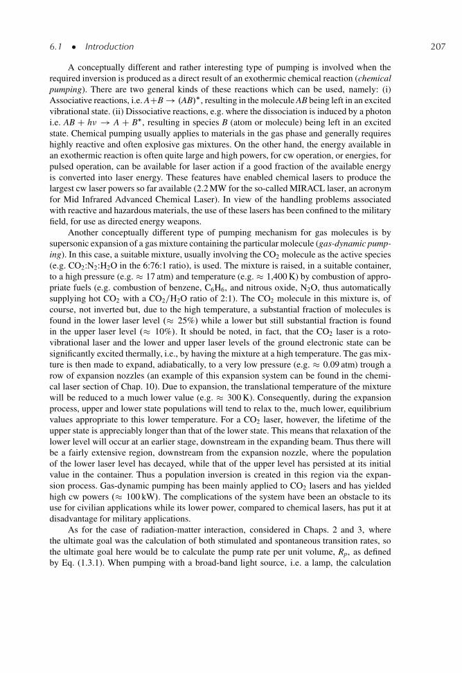
6.1 � Introduction 207
A conceptually different and rather interesting type of pumping is involved when therequired inversion is produced as a direct result of an exothermic chemical reaction (chemicalpumping). There are two general kinds of these reactions which can be used, namely: (i)Associative reactions, i.e. ACB ! .AB/�, resulting in the molecule AB being left in an excitedvibrational state. (ii) Dissociative reactions, e.g. where the dissociation is induced by a photoni.e. AB C h� ! A C B�, resulting in species B (atom or molecule) being left in an excitedstate. Chemical pumping usually applies to materials in the gas phase and generally requireshighly reactive and often explosive gas mixtures. On the other hand, the energy available inan exothermic reaction is often quite large and high powers, for cw operation, or energies, forpulsed operation, can be available for laser action if a good fraction of the available energyis converted into laser energy. These features have enabled chemical lasers to produce thelargest cw laser powers so far available (2.2 MW for the so-called MIRACL laser, an acronymfor Mid Infrared Advanced Chemical Laser). In view of the handling problems associatedwith reactive and hazardous materials, the use of these lasers has been confined to the militaryfield, for use as directed energy weapons.
Another conceptually different type of pumping mechanism for gas molecules is bysupersonic expansion of a gas mixture containing the particular molecule (gas-dynamic pump-ing). In this case, a suitable mixture, usually involving the CO2 molecule as the active species(e.g. CO2:N2:H2O in the 6:76:1 ratio), is used. The mixture is raised, in a suitable container,to a high pressure (e.g. � 17 atm) and temperature (e.g. � 1,400 K) by combustion of appro-priate fuels (e.g. combustion of benzene, C6H6, and nitrous oxide, N2O, thus automaticallysupplying hot CO2 with a CO2=H2O ratio of 2:1). The CO2 molecule in this mixture is, ofcourse, not inverted but, due to the high temperature, a substantial fraction of molecules isfound in the lower laser level .� 25%/ while a lower but still substantial fraction is foundin the upper laser level .� 10%/. It should be noted, in fact, that the CO2 laser is a roto-vibrational laser and the lower and upper laser levels of the ground electronic state can besignificantly excited thermally, i.e., by having the mixture at a high temperature. The gas mix-ture is then made to expand, adiabatically, to a very low pressure (e.g. � 0.09 atm) trough arow of expansion nozzles (an example of this expansion system can be found in the chemi-cal laser section of Chap. 10). Due to expansion, the translational temperature of the mixturewill be reduced to a much lower value (e.g. � 300 K). Consequently, during the expansionprocess, upper and lower state populations will tend to relax to the, much lower, equilibriumvalues appropriate to this lower temperature. For a CO2 laser, however, the lifetime of theupper state is appreciably longer than that of the lower state. This means that relaxation of thelower level will occur at an earlier stage, downstream in the expanding beam. Thus there willbe a fairly extensive region, downstream from the expansion nozzle, where the populationof the lower laser level has decayed, while that of the upper level has persisted at its initialvalue in the container. Thus a population inversion is created in this region via the expan-sion process. Gas-dynamic pumping has been mainly applied to CO2 lasers and has yieldedhigh cw powers .� 100 kW/. The complications of the system have been an obstacle to itsuse for civilian applications while its lower power, compared to chemical lasers, has put it atdisadvantage for military applications.
As for the case of radiation-matter interaction, considered in Chaps. 2 and 3, wherethe ultimate goal was the calculation of both stimulated and spontaneous transition rates, sothe ultimate goal here would be to calculate the pump rate per unit volume, Rp, as definedby Eq. (1.3.1). When pumping with a broad-band light source, i.e. a lamp, the calculation
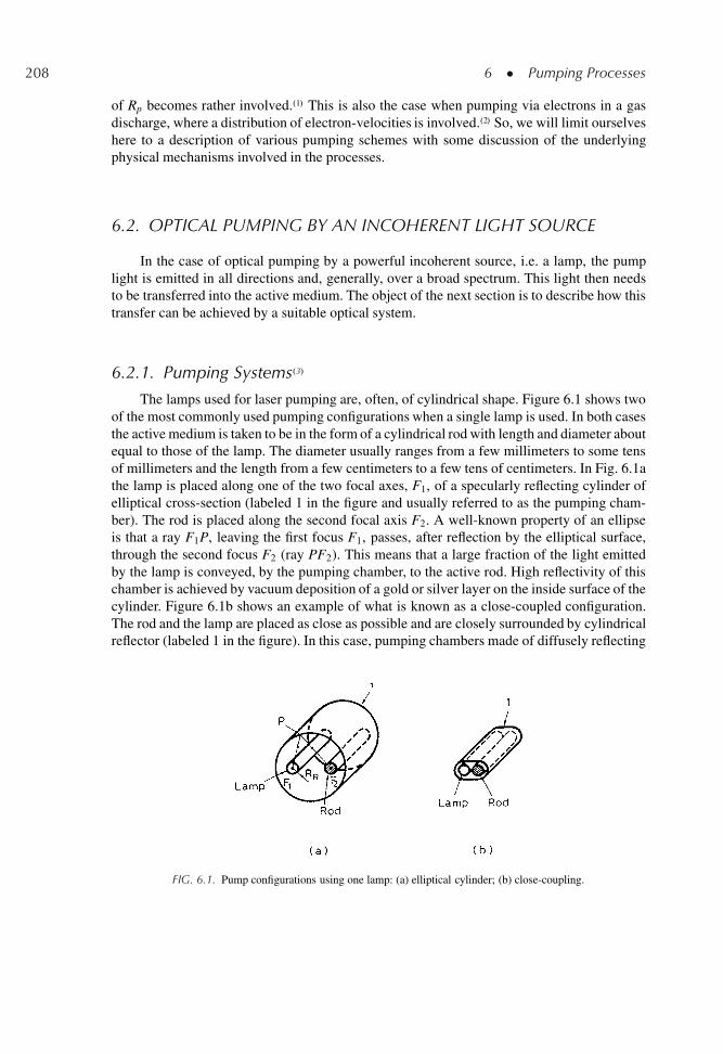
208 6 � Pumping Processes
of Rp becomes rather involved..1/ This is also the case when pumping via electrons in a gasdischarge, where a distribution of electron-velocities is involved..2/ So, we will limit ourselveshere to a description of various pumping schemes with some discussion of the underlyingphysical mechanisms involved in the processes.
6.2. OPTICAL PUMPING BY AN INCOHERENT LIGHT SOURCE
In the case of optical pumping by a powerful incoherent source, i.e. a lamp, the pumplight is emitted in all directions and, generally, over a broad spectrum. This light then needsto be transferred into the active medium. The object of the next section is to describe how thistransfer can be achieved by a suitable optical system.
6.2.1. Pumping Systems.3/
The lamps used for laser pumping are, often, of cylindrical shape. Figure 6.1 shows twoof the most commonly used pumping configurations when a single lamp is used. In both casesthe active medium is taken to be in the form of a cylindrical rod with length and diameter aboutequal to those of the lamp. The diameter usually ranges from a few millimeters to some tensof millimeters and the length from a few centimeters to a few tens of centimeters. In Fig. 6.1athe lamp is placed along one of the two focal axes, F1, of a specularly reflecting cylinder ofelliptical cross-section (labeled 1 in the figure and usually referred to as the pumping cham-ber). The rod is placed along the second focal axis F2. A well-known property of an ellipseis that a ray F1P, leaving the first focus F1, passes, after reflection by the elliptical surface,through the second focus F2 (ray PF2). This means that a large fraction of the light emittedby the lamp is conveyed, by the pumping chamber, to the active rod. High reflectivity of thischamber is achieved by vacuum deposition of a gold or silver layer on the inside surface of thecylinder. Figure 6.1b shows an example of what is known as a close-coupled configuration.The rod and the lamp are placed as close as possible and are closely surrounded by cylindricalreflector (labeled 1 in the figure). In this case, pumping chambers made of diffusely reflecting
FIG. 6.1. Pump configurations using one lamp: (a) elliptical cylinder; (b) close-coupling.
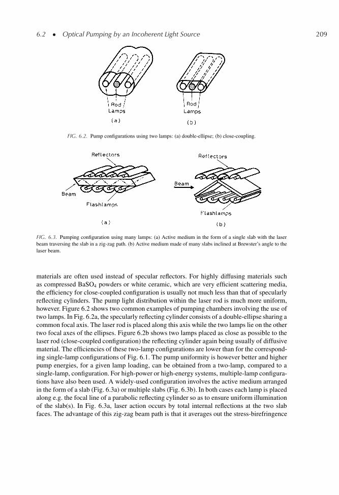
6.2 � Optical Pumping by an Incoherent Light Source 209
FIG. 6.2. Pump configurations using two lamps: (a) double-ellipse; (b) close-coupling.
FIG. 6.3. Pumping configuration using many lamps: (a) Active medium in the form of a single slab with the laserbeam traversing the slab in a zig-zag path. (b) Active medium made of many slabs inclined at Brewster’s angle to thelaser beam.
materials are often used instead of specular reflectors. For highly diffusing materials suchas compressed BaSO4 powders or white ceramic, which are very efficient scattering media,the efficiency for close-coupled configuration is usually not much less than that of specularlyreflecting cylinders. The pump light distribution within the laser rod is much more uniform,however. Figure 6.2 shows two common examples of pumping chambers involving the use oftwo lamps. In Fig. 6.2a, the specularly reflecting cylinder consists of a double-ellipse sharing acommon focal axis. The laser rod is placed along this axis while the two lamps lie on the othertwo focal axes of the ellipses. Figure 6.2b shows two lamps placed as close as possible to thelaser rod (close-coupled configuration) the reflecting cylinder again being usually of diffusivematerial. The efficiencies of these two-lamp configurations are lower than for the correspond-ing single-lamp configurations of Fig. 6.1. The pump uniformity is however better and higherpump energies, for a given lamp loading, can be obtained from a two-lamp, compared to asingle-lamp, configuration. For high-power or high-energy systems, multiple-lamp configura-tions have also been used. A widely-used configuration involves the active medium arrangedin the form of a slab (Fig. 6.3a) or multiple slabs (Fig. 6.3b). In both cases each lamp is placedalong e.g. the focal line of a parabolic reflecting cylinder so as to ensure uniform illuminationof the slab(s). In Fig. 6.3a, laser action occurs by total internal reflections at the two slabfaces. The advantage of this zig-zag beam path is that it averages out the stress-birefringence
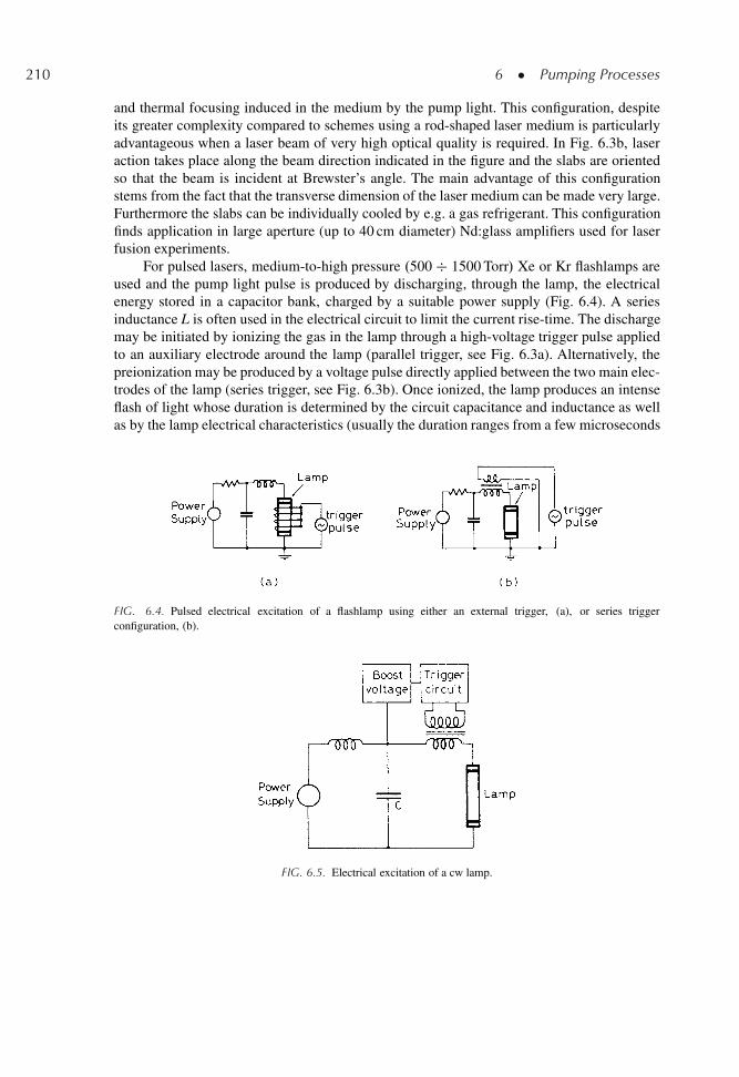
210 6 � Pumping Processes
and thermal focusing induced in the medium by the pump light. This configuration, despiteits greater complexity compared to schemes using a rod-shaped laser medium is particularlyadvantageous when a laser beam of very high optical quality is required. In Fig. 6.3b, laseraction takes place along the beam direction indicated in the figure and the slabs are orientedso that the beam is incident at Brewster’s angle. The main advantage of this configurationstems from the fact that the transverse dimension of the laser medium can be made very large.Furthermore the slabs can be individually cooled by e.g. a gas refrigerant. This configurationfinds application in large aperture (up to 40 cm diameter) Nd:glass amplifiers used for laserfusion experiments.
For pulsed lasers, medium-to-high pressure .500 � 1500 Torr/ Xe or Kr flashlamps areused and the pump light pulse is produced by discharging, through the lamp, the electricalenergy stored in a capacitor bank, charged by a suitable power supply (Fig. 6.4). A seriesinductance L is often used in the electrical circuit to limit the current rise-time. The dischargemay be initiated by ionizing the gas in the lamp through a high-voltage trigger pulse appliedto an auxiliary electrode around the lamp (parallel trigger, see Fig. 6.3a). Alternatively, thepreionization may be produced by a voltage pulse directly applied between the two main elec-trodes of the lamp (series trigger, see Fig. 6.3b). Once ionized, the lamp produces an intenseflash of light whose duration is determined by the circuit capacitance and inductance as wellas by the lamp electrical characteristics (usually the duration ranges from a few microseconds
FIG. 6.4. Pulsed electrical excitation of a flashlamp using either an external trigger, (a), or series triggerconfiguration, (b).
FIG. 6.5. Electrical excitation of a cw lamp.
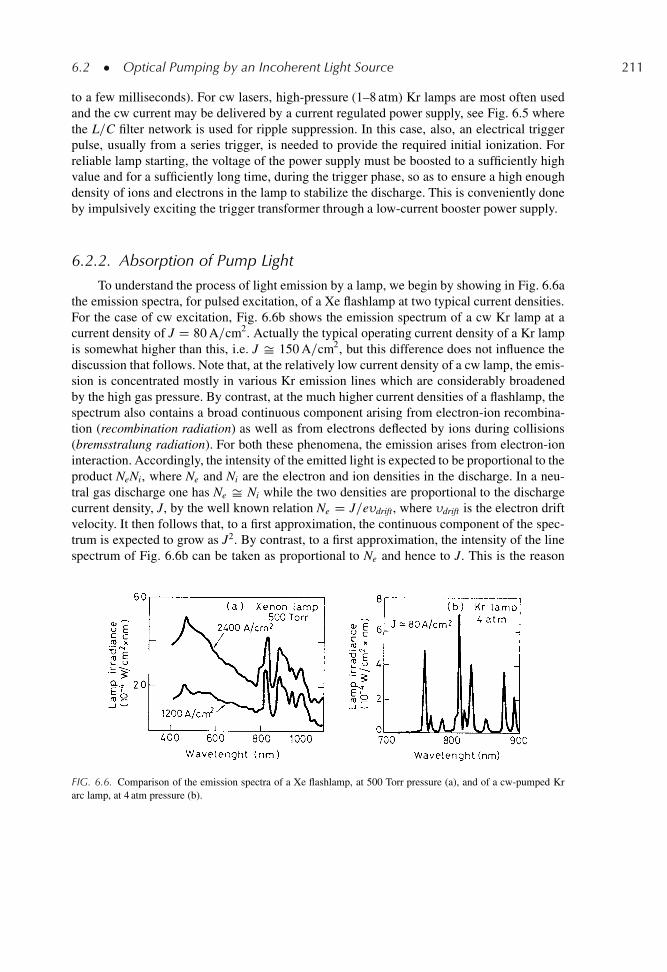
6.2 � Optical Pumping by an Incoherent Light Source 211
to a few milliseconds). For cw lasers, high-pressure (1–8 atm) Kr lamps are most often usedand the cw current may be delivered by a current regulated power supply, see Fig. 6.5 wherethe L=C filter network is used for ripple suppression. In this case, also, an electrical triggerpulse, usually from a series trigger, is needed to provide the required initial ionization. Forreliable lamp starting, the voltage of the power supply must be boosted to a sufficiently highvalue and for a sufficiently long time, during the trigger phase, so as to ensure a high enoughdensity of ions and electrons in the lamp to stabilize the discharge. This is conveniently doneby impulsively exciting the trigger transformer through a low-current booster power supply.
6.2.2. Absorption of Pump Light
To understand the process of light emission by a lamp, we begin by showing in Fig. 6.6athe emission spectra, for pulsed excitation, of a Xe flashlamp at two typical current densities.For the case of cw excitation, Fig. 6.6b shows the emission spectrum of a cw Kr lamp at acurrent density of J D 80 A=cm2. Actually the typical operating current density of a Kr lampis somewhat higher than this, i.e. J Š 150 A=cm2, but this difference does not influence thediscussion that follows. Note that, at the relatively low current density of a cw lamp, the emis-sion is concentrated mostly in various Kr emission lines which are considerably broadenedby the high gas pressure. By contrast, at the much higher current densities of a flashlamp, thespectrum also contains a broad continuous component arising from electron-ion recombina-tion (recombination radiation) as well as from electrons deflected by ions during collisions(bremsstralung radiation). For both these phenomena, the emission arises from electron-ioninteraction. Accordingly, the intensity of the emitted light is expected to be proportional to theproduct NeNi, where Ne and Ni are the electron and ion densities in the discharge. In a neu-tral gas discharge one has Ne Š Ni while the two densities are proportional to the dischargecurrent density, J, by the well known relation Ne D J=e�drift, where �drift is the electron driftvelocity. It then follows that, to a first approximation, the continuous component of the spec-trum is expected to grow as J2. By contrast, to a first approximation, the intensity of the linespectrum of Fig. 6.6b can be taken as proportional to Ne and hence to J. This is the reason
FIG. 6.6. Comparison of the emission spectra of a Xe flashlamp, at 500 Torr pressure (a), and of a cw-pumped Krarc lamp, at 4 atm pressure (b).
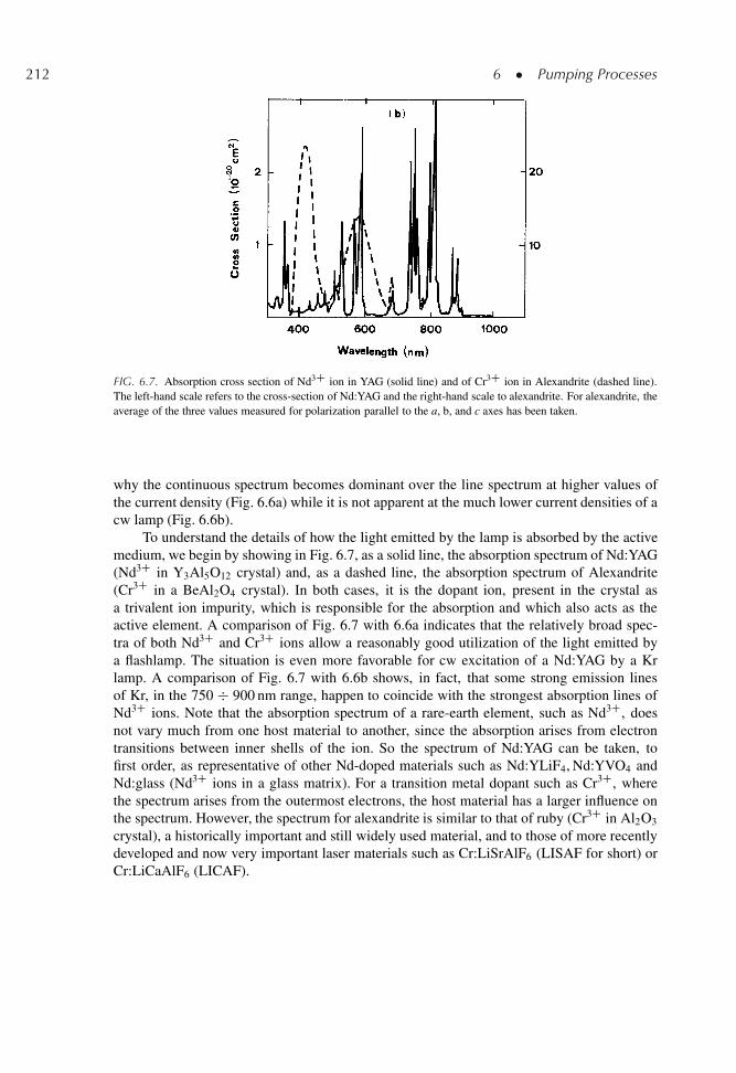
212 6 � Pumping Processes
FIG. 6.7. Absorption cross section of Nd3C ion in YAG (solid line) and of Cr3C ion in Alexandrite (dashed line).The left-hand scale refers to the cross-section of Nd:YAG and the right-hand scale to alexandrite. For alexandrite, theaverage of the three values measured for polarization parallel to the a, b, and c axes has been taken.
why the continuous spectrum becomes dominant over the line spectrum at higher values ofthe current density (Fig. 6.6a) while it is not apparent at the much lower current densities of acw lamp (Fig. 6.6b).
To understand the details of how the light emitted by the lamp is absorbed by the activemedium, we begin by showing in Fig. 6.7, as a solid line, the absorption spectrum of Nd:YAG(Nd3C in Y3Al5O12 crystal) and, as a dashed line, the absorption spectrum of Alexandrite(Cr3C in a BeAl2O4 crystal). In both cases, it is the dopant ion, present in the crystal asa trivalent ion impurity, which is responsible for the absorption and which also acts as theactive element. A comparison of Fig. 6.7 with 6.6a indicates that the relatively broad spec-tra of both Nd3C and Cr3C ions allow a reasonably good utilization of the light emitted bya flashlamp. The situation is even more favorable for cw excitation of a Nd:YAG by a Krlamp. A comparison of Fig. 6.7 with 6.6b shows, in fact, that some strong emission linesof Kr, in the 750 � 900 nm range, happen to coincide with the strongest absorption lines ofNd3C ions. Note that the absorption spectrum of a rare-earth element, such as Nd3C, doesnot vary much from one host material to another, since the absorption arises from electrontransitions between inner shells of the ion. So the spectrum of Nd:YAG can be taken, tofirst order, as representative of other Nd-doped materials such as Nd:YLiF4, Nd:YVO4 andNd:glass (Nd3C ions in a glass matrix). For a transition metal dopant such as Cr3C, wherethe spectrum arises from the outermost electrons, the host material has a larger influence onthe spectrum. However, the spectrum for alexandrite is similar to that of ruby (Cr3C in Al2O3
crystal), a historically important and still widely used material, and to those of more recentlydeveloped and now very important laser materials such as Cr:LiSrAlF6 (LISAF for short) orCr:LiCaAlF6 (LICAF).
6.2 � Optical Pumping by an Incoherent Light Source 213
6.2.3. Pump Efficiency and Pump Rate
Consider first a cw laser pumped by a pump rate, Rp, which is assumed uniform troughoutthe volume of the pumped region, V . We can ask ourselves what would be the minimum pumppower, Pm, needed to obtain a given pump rate Rp. With reference to Fig. 6.17, this wouldcorrespond to the case where the upper laser level were directly pumped from the ground stateby, e.g. monochromatic pump photons of energy h�mp, where �mp is the frequency differencebetween the ground level and the upper laser level. The minimum pump power, Pm, is thengiven by
Pm D .dN2=dt/pV h�mp D RpV h�mp (6.2.1a)
where V is the pumped volume of the active medium. We can now define a pump efficiency,�p, as the ratio between this minimum pump power, Pm, and the actual electrical pump power,Pp, entering the lamp i.e.
�p D Pm=Pp (6.2.1)
For non-uniform pumping, we can then write
Pm D h �mpRa
RpdV DD h �mp<Rp>V
(6.2.2)
where the integral is taken over the whole volume of the medium and <Rp> is the average ofRp in the medium. From Eqs. (6.2.1) and (6.2.2) we then get
�p D .h �mp<Rp>V/=Pp (6.2.3)
For a pulsed pumping system, we can, likewise, define �p as
�p D .h�mp
ZRpdVdt/=Ep (6.2.4)
where the integral is also taken over the whole duration of the pump pulse and Ep is theelectrical pump energy given to the lamp.
To calculate or simply estimate the pumping efficiency, the pump process can be dividedinto four distinct steps: (i) the emission of radiation by the lamp; (ii) the transfer of this radia-tion to the active medium; (iii) the absorption in the medium; (iv) the transfer of the absorbedradiation to the upper laser level. Consequently, the pumping efficiency can be written as theproduct of four terms, namely,
�p D Pr
Pp
Pt
Pr
Pa
Pt
Pm
PaD �r�t�a�pq (6.2.5)
where: (i) �r D Pr=Pp is the ratio between the radiated power of the lamp in the wavelengthrange corresponding to the pump bands of the laser medium, Pr, and the total electrical pump
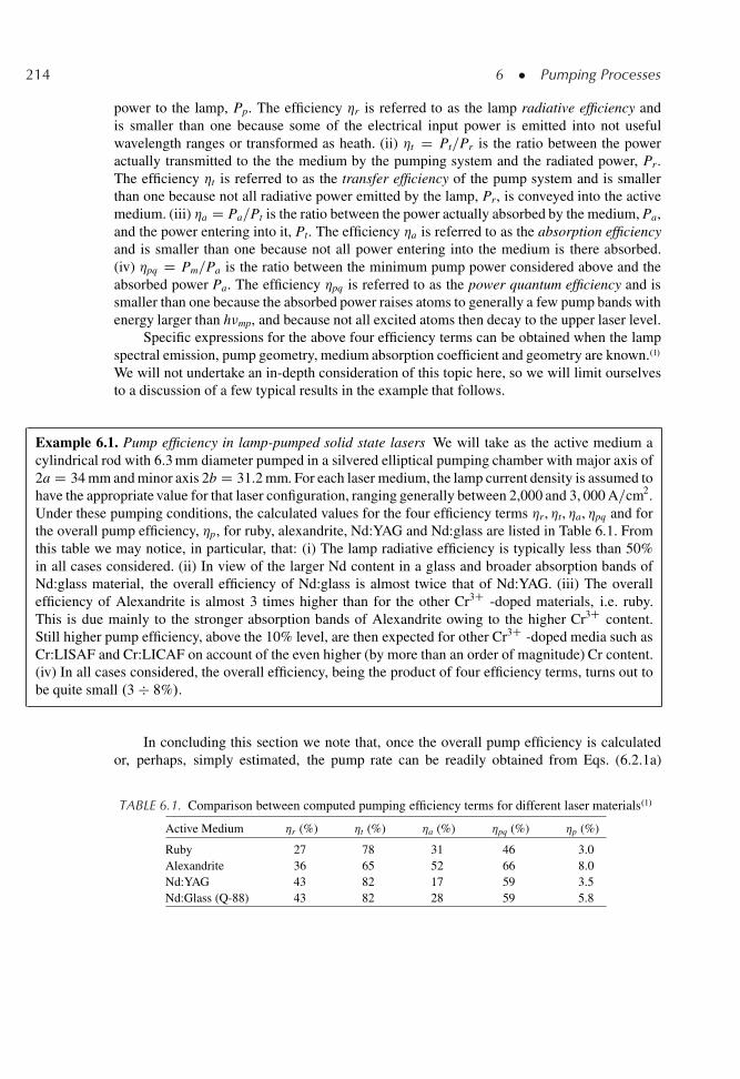
214 6 � Pumping Processes
power to the lamp, Pp. The efficiency �r is referred to as the lamp radiative efficiency andis smaller than one because some of the electrical input power is emitted into not usefulwavelength ranges or transformed as heath. (ii) �t D Pt=Pr is the ratio between the poweractually transmitted to the the medium by the pumping system and the radiated power, Pr.The efficiency �t is referred to as the transfer efficiency of the pump system and is smallerthan one because not all radiative power emitted by the lamp, Pr, is conveyed into the activemedium. (iii) �a D Pa=Pt is the ratio between the power actually absorbed by the medium, Pa,and the power entering into it, Pt. The efficiency �a is referred to as the absorption efficiencyand is smaller than one because not all power entering into the medium is there absorbed.(iv) �pq D Pm=Pa is the ratio between the minimum pump power considered above and theabsorbed power Pa. The efficiency �pq is referred to as the power quantum efficiency and issmaller than one because the absorbed power raises atoms to generally a few pump bands withenergy larger than h�mp, and because not all excited atoms then decay to the upper laser level.
Specific expressions for the above four efficiency terms can be obtained when the lampspectral emission, pump geometry, medium absorption coefficient and geometry are known..1/
We will not undertake an in-depth consideration of this topic here, so we will limit ourselvesto a discussion of a few typical results in the example that follows.
Example 6.1. Pump efficiency in lamp-pumped solid state lasers We will take as the active medium acylindrical rod with 6.3 mm diameter pumped in a silvered elliptical pumping chamber with major axis of2a D 34 mm and minor axis 2b D 31.2 mm. For each laser medium, the lamp current density is assumed tohave the appropriate value for that laser configuration, ranging generally between 2,000 and 3, 000 A=cm2.Under these pumping conditions, the calculated values for the four efficiency terms �r, �t, �a, �pq and forthe overall pump efficiency, �p, for ruby, alexandrite, Nd:YAG and Nd:glass are listed in Table 6.1. Fromthis table we may notice, in particular, that: (i) The lamp radiative efficiency is typically less than 50%in all cases considered. (ii) In view of the larger Nd content in a glass and broader absorption bands ofNd:glass material, the overall efficiency of Nd:glass is almost twice that of Nd:YAG. (iii) The overallefficiency of Alexandrite is almost 3 times higher than for the other Cr3C -doped materials, i.e. ruby.This is due mainly to the stronger absorption bands of Alexandrite owing to the higher Cr3C content.Still higher pump efficiency, above the 10% level, are then expected for other Cr3C -doped media such asCr:LISAF and Cr:LICAF on account of the even higher (by more than an order of magnitude) Cr content.(iv) In all cases considered, the overall efficiency, being the product of four efficiency terms, turns out tobe quite small .3 � 8%/.
In concluding this section we note that, once the overall pump efficiency is calculatedor, perhaps, simply estimated, the pump rate can be readily obtained from Eqs. (6.2.1a)
TABLE 6.1. Comparison between computed pumping efficiency terms for different laser materials.1/
Active Medium �r (%) �t (%) �a (%) �pq (%) �p (%)
Ruby 27 78 31 46 3.0Alexandrite 36 65 52 66 8.0Nd:YAG 43 82 17 59 3.5Nd:Glass (Q-88) 43 82 28 59 5.8
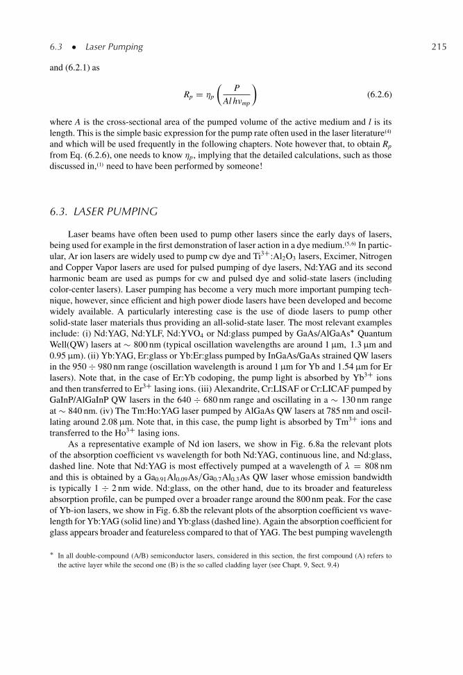
6.3 � Laser Pumping 215
and (6.2.1) as
Rp D �p
�P
Al h�mp
�(6.2.6)
where A is the cross-sectional area of the pumped volume of the active medium and l is itslength. This is the simple basic expression for the pump rate often used in the laser literature.4/
and which will be used frequently in the following chapters. Note however that, to obtain Rp
from Eq. (6.2.6), one needs to know �p, implying that the detailed calculations, such as thosediscussed in,.1/ need to have been performed by someone!
6.3. LASER PUMPING
Laser beams have often been used to pump other lasers since the early days of lasers,being used for example in the first demonstration of laser action in a dye medium..5,6/ In partic-ular, Ar ion lasers are widely used to pump cw dye and Ti3C:Al2O3 lasers, Excimer, Nitrogenand Copper Vapor lasers are used for pulsed pumping of dye lasers, Nd:YAG and its secondharmonic beam are used as pumps for cw and pulsed dye and solid-state lasers (includingcolor-center lasers). Laser pumping has become a very much more important pumping tech-nique, however, since efficient and high power diode lasers have been developed and becomewidely available. A particularly interesting case is the use of diode lasers to pump othersolid-state laser materials thus providing an all-solid-state laser. The most relevant examplesinclude: (i) Nd:YAG, Nd:YLF, Nd:YVO4 or Nd:glass pumped by GaAs/AlGaAs� QuantumWell(QW) lasers at � 800 nm (typical oscillation wavelengths are around 1 μm, 1.3 μm and0.95 μm). (ii) Yb:YAG, Er:glass or Yb:Er:glass pumped by InGaAs/GaAs strained QW lasersin the 950 � 980 nm range (oscillation wavelength is around 1 μm for Yb and 1.54 μm for Erlasers). Note that, in the case of Er:Yb codoping, the pump light is absorbed by Yb3C ionsand then transferred to Er3C lasing ions. (iii) Alexandrite, Cr:LISAF or Cr:LICAF pumped byGaInP/AlGaInP QW lasers in the 640 � 680 nm range and oscillating in a � 130 nm rangeat � 840 nm. (iv) The Tm:Ho:YAG laser pumped by AlGaAs QW lasers at 785 nm and oscil-lating around 2.08 μm. Note that, in this case, the pump light is absorbed by Tm3C ions andtransferred to the Ho3C lasing ions.
As a representative example of Nd ion lasers, we show in Fig. 6.8a the relevant plotsof the absorption coefficient vs wavelength for both Nd:YAG, continuous line, and Nd:glass,dashed line. Note that Nd:YAG is most effectively pumped at a wavelength of � D 808 nmand this is obtained by a Ga0.91Al0.09As=Ga0.7Al0.3As QW laser whose emission bandwidthis typically 1 � 2 nm wide. Nd:glass, on the other hand, due to its broader and featurelessabsorption profile, can be pumped over a broader range around the 800 nm peak. For the caseof Yb-ion lasers, we show in Fig. 6.8b the relevant plots of the absorption coefficient vs wave-length for Yb:YAG (solid line) and Yb:glass (dashed line). Again the absorption coefficient forglass appears broader and featureless compared to that of YAG. The best pumping wavelength
� In all double-compound (A/B) semiconductor lasers, considered in this section, the first compound (A) refers tothe active layer while the second one (B) is the so called cladding layer (see Chapt. 9, Sect. 9.4)
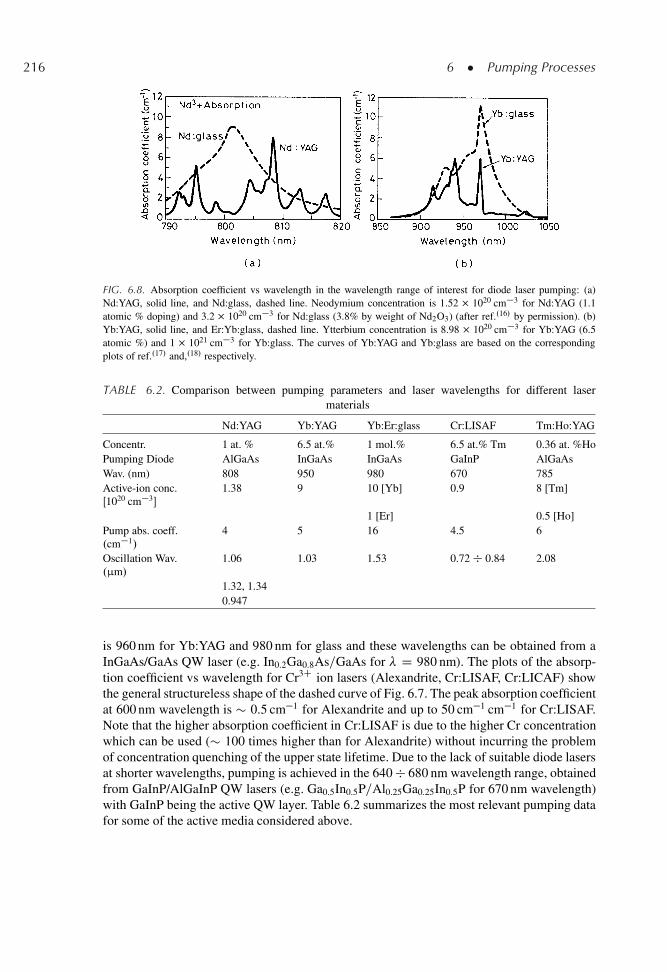
216 6 � Pumping Processes
FIG. 6.8. Absorption coefficient vs wavelength in the wavelength range of interest for diode laser pumping: (a)Nd:YAG, solid line, and Nd:glass, dashed line. Neodymium concentration is 1.52 1020 cm�3 for Nd:YAG (1.1atomic % doping) and 3.2 1020 cm�3 for Nd:glass (3.8% by weight of Nd2O3) (after ref..16/ by permission). (b)Yb:YAG, solid line, and Er:Yb:glass, dashed line. Ytterbium concentration is 8.98 1020 cm�3 for Yb:YAG (6.5atomic %) and 1 1021 cm�3 for Yb:glass. The curves of Yb:YAG and Yb:glass are based on the correspondingplots of ref..17/ and,.18/ respectively.
TABLE 6.2. Comparison between pumping parameters and laser wavelengths for different lasermaterials
Nd:YAG Yb:YAG Yb:Er:glass Cr:LISAF Tm:Ho:YAG
Concentr. 1 at. % 6.5 at.% 1 mol.% 6.5 at.% Tm 0.36 at. %HoPumping Diode AlGaAs InGaAs InGaAs GaInP AlGaAsWav. (nm) 808 950 980 670 785Active-ion conc.Œ1020 cm�3�
1.38 9 10 [Yb] 0.9 8 [Tm]
1 [Er] 0.5 [Ho]Pump abs. coeff..cm�1/
4 5 16 4.5 6
Oscillation Wav..μm/
1.06 1.03 1.53 0.72 � 0.84 2.08
1.32, 1.340.947
is 960 nm for Yb:YAG and 980 nm for glass and these wavelengths can be obtained from aInGaAs/GaAs QW laser (e.g. In0.2Ga0.8As=GaAs for � D 980 nm). The plots of the absorp-tion coefficient vs wavelength for Cr3C ion lasers (Alexandrite, Cr:LISAF, Cr:LICAF) showthe general structureless shape of the dashed curve of Fig. 6.7. The peak absorption coefficientat 600 nm wavelength is � 0.5 cm�1 for Alexandrite and up to 50 cm�1 cm�1 for Cr:LISAF.Note that the higher absorption coefficient in Cr:LISAF is due to the higher Cr concentrationwhich can be used (� 100 times higher than for Alexandrite) without incurring the problemof concentration quenching of the upper state lifetime. Due to the lack of suitable diode lasersat shorter wavelengths, pumping is achieved in the 640 � 680 nm wavelength range, obtainedfrom GaInP/AlGaInP QW lasers (e.g. Ga0.5In0.5P=Al0.25Ga0.25In0.5P for 670 nm wavelength)with GaInP being the active QW layer. Table 6.2 summarizes the most relevant pumping datafor some of the active media considered above.
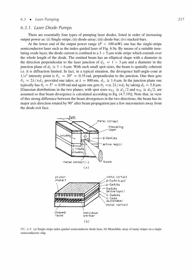
6.3 � Laser Pumping 217
6.3.1. Laser Diode Pumps
There are essentially four types of pumping laser diodes, listed in order of increasingoutput power as: (i) Single-stripe; (ii) diode-array; (iii) diode-bar; (iv) stacked-bars.
At the lower end of the output power range .P < 100 mW/ one has the single-stripesemiconductor laser such as the index-guided laser of Fig. 6.9a. By means of a suitable insu-lating oxide layer, the diode current is confined to a 3 � 5 μm wide stripe which extends overthe whole length of the diode. The emitted beam has an elliptical shape with a diameter inthe direction perpendicular to the laser junction of d? D 1 � 3 μm and a diameter in thejunction plane of djj Š 3 � 6 μm. With such small spot-sizes, the beam is spatially coherenti.e. it is diffraction limited. In fact, in a typical situation, the divergence half-angle-cone at1=e2 intensity point is ? D 20ı D 0.35 rad, perpendicular to the junction. One then gets? D 2�= d? provided one takes, at � D 800 nm, d? Š 1.4 μm. In the junction plane onetypically has jj D 5ı D 0.09 rad and again one gets jj DŠ 2�= djj by taking djj D 5.8 μm.[Gaussian distributions in the two planes, with spot sizes w0? Š d?=2 and w0jj Š djj=2, areassumed so that beam divergence is calculated according to Eq. (4.7.19)]. Note that, in viewof this strong difference between the beam divergences in the two directions, the beam has itsmajor axis direction rotated by 90ı after beam propagation just a few micrometers away fromthe diode exit face.
FIG. 6.9. (a) Single-stripe index-guided semiconductor diode laser. (b) Monolithic array of many stripes on a singlesemiconductors chip.
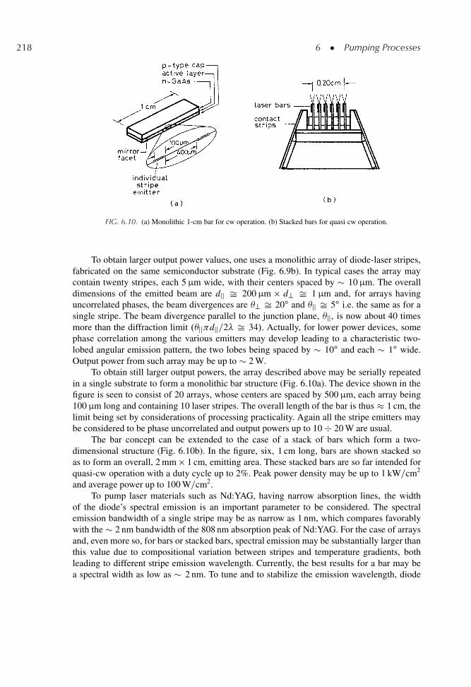
218 6 � Pumping Processes
FIG. 6.10. (a) Monolithic 1-cm bar for cw operation. (b) Stacked bars for quasi cw operation.
To obtain larger output power values, one uses a monolithic array of diode-laser stripes,fabricated on the same semiconductor substrate (Fig. 6.9b). In typical cases the array maycontain twenty stripes, each 5 μm wide, with their centers spaced by � 10 μm. The overalldimensions of the emitted beam are djj Š 200 μm � d? Š 1 μm and, for arrays havinguncorrelated phases, the beam divergences are ? Š 20ı and jj Š 5ı i.e. the same as for asingle stripe. The beam divergence parallel to the junction plane, jj, is now about 40 timesmore than the diffraction limit .jj djj=2� Š 34/. Actually, for lower power devices, somephase correlation among the various emitters may develop leading to a characteristic two-lobed angular emission pattern, the two lobes being spaced by � 10ı and each � 1ı wide.Output power from such array may be up to � 2 W.
To obtain still larger output powers, the array described above may be serially repeatedin a single substrate to form a monolithic bar structure (Fig. 6.10a). The device shown in thefigure is seen to consist of 20 arrays, whose centers are spaced by 500 μm, each array being100 μm long and containing 10 laser stripes. The overall length of the bar is thus � 1 cm, thelimit being set by considerations of processing practicality. Again all the stripe emitters maybe considered to be phase uncorrelated and output powers up to 10 � 20 W are usual.
The bar concept can be extended to the case of a stack of bars which form a two-dimensional structure (Fig. 6.10b). In the figure, six, 1 cm long, bars are shown stacked soas to form an overall, 2 mm � 1 cm, emitting area. These stacked bars are so far intended forquasi-cw operation with a duty cycle up to 2%. Peak power density may be up to 1 kW=cm2
and average power up to 100 W=cm2.To pump laser materials such as Nd:YAG, having narrow absorption lines, the width
of the diode’s spectral emission is an important parameter to be considered. The spectralemission bandwidth of a single stripe may be as narrow as 1 nm, which compares favorablywith the � 2 nm bandwidth of the 808 nm absorption peak of Nd:YAG. For the case of arraysand, even more so, for bars or stacked bars, spectral emission may be substantially larger thanthis value due to compositional variation between stripes and temperature gradients, bothleading to different stripe emission wavelength. Currently, the best results for a bar may bea spectral width as low as � 2 nm. To tune and to stabilize the emission wavelength, diode
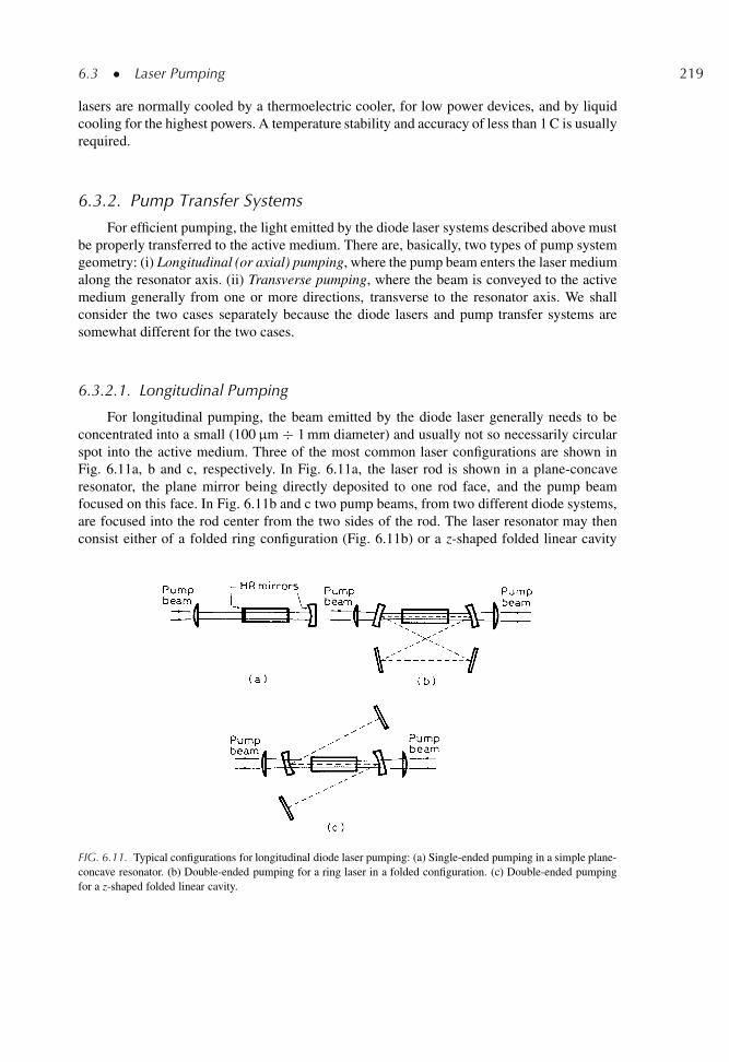
6.3 � Laser Pumping 219
lasers are normally cooled by a thermoelectric cooler, for low power devices, and by liquidcooling for the highest powers. A temperature stability and accuracy of less than 1 C is usuallyrequired.
6.3.2. Pump Transfer Systems
For efficient pumping, the light emitted by the diode laser systems described above mustbe properly transferred to the active medium. There are, basically, two types of pump systemgeometry: (i) Longitudinal (or axial) pumping, where the pump beam enters the laser mediumalong the resonator axis. (ii) Transverse pumping, where the beam is conveyed to the activemedium generally from one or more directions, transverse to the resonator axis. We shallconsider the two cases separately because the diode lasers and pump transfer systems aresomewhat different for the two cases.
6.3.2.1. Longitudinal Pumping
For longitudinal pumping, the beam emitted by the diode laser generally needs to beconcentrated into a small (100 μm � 1 mm diameter) and usually not so necessarily circularspot into the active medium. Three of the most common laser configurations are shown inFig. 6.11a, b and c, respectively. In Fig. 6.11a, the laser rod is shown in a plane-concaveresonator, the plane mirror being directly deposited to one rod face, and the pump beamfocused on this face. In Fig. 6.11b and c two pump beams, from two different diode systems,are focused into the rod center from the two sides of the rod. The laser resonator may thenconsist either of a folded ring configuration (Fig. 6.11b) or a z-shaped folded linear cavity
FIG. 6.11. Typical configurations for longitudinal diode laser pumping: (a) Single-ended pumping in a simple plane-concave resonator. (b) Double-ended pumping for a ring laser in a folded configuration. (c) Double-ended pumpingfor a z-shaped folded linear cavity.
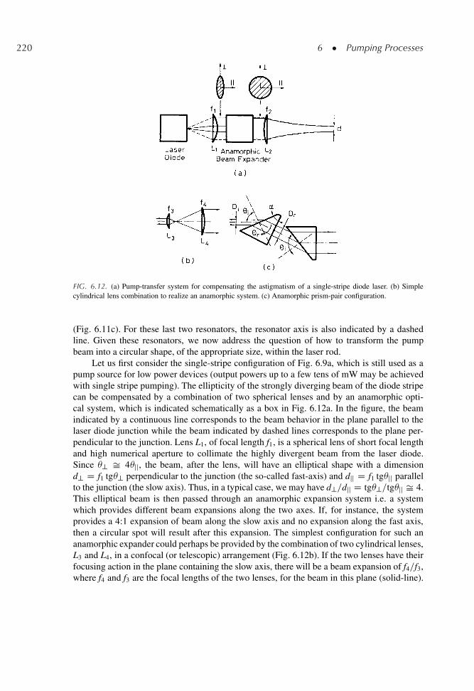
220 6 � Pumping Processes
FIG. 6.12. (a) Pump-transfer system for compensating the astigmatism of a single-stripe diode laser. (b) Simplecylindrical lens combination to realize an anamorphic system. (c) Anamorphic prism-pair configuration.
(Fig. 6.11c). For these last two resonators, the resonator axis is also indicated by a dashedline. Given these resonators, we now address the question of how to transform the pumpbeam into a circular shape, of the appropriate size, within the laser rod.
Let us first consider the single-stripe configuration of Fig. 6.9a, which is still used as apump source for low power devices (output powers up to a few tens of mW may be achievedwith single stripe pumping). The ellipticity of the strongly diverging beam of the diode stripecan be compensated by a combination of two spherical lenses and by an anamorphic opti-cal system, which is indicated schematically as a box in Fig. 6.12a. In the figure, the beamindicated by a continuous line corresponds to the beam behavior in the plane parallel to thelaser diode junction while the beam indicated by dashed lines corresponds to the plane per-pendicular to the junction. Lens L1, of focal length f1, is a spherical lens of short focal lengthand high numerical aperture to collimate the highly divergent beam from the laser diode.Since ? Š 4jj, the beam, after the lens, will have an elliptical shape with a dimensiond? D f1 tg? perpendicular to the junction (the so-called fast-axis) and djj D f1 tgjj parallelto the junction (the slow axis). Thus, in a typical case, we may have d?=djj D tg?=tgjj Š 4.This elliptical beam is then passed through an anamorphic expansion system i.e. a systemwhich provides different beam expansions along the two axes. If, for instance, the systemprovides a 4:1 expansion of beam along the slow axis and no expansion along the fast axis,then a circular spot will result after this expansion. The simplest configuration for such ananamorphic expander could perhaps be provided by the combination of two cylindrical lenses,L3 and L4, in a confocal (or telescopic) arrangement (Fig. 6.12b). If the two lenses have theirfocusing action in the plane containing the slow axis, there will be a beam expansion of f4=f3,where f4 and f3 are the focal lengths of the two lenses, for the beam in this plane (solid-line).
6.3 � Laser Pumping 221
For the other plane, however, the two cylindrical lenses behave simply as plane parallel platesand the beam will thus be unaffected, in the fast-axis direction, by the beam expander. Theanamorphic system of Fig. 6.12b is seldom used in practice, however, because, to save space,the system would require cylindrical lenses of short focal length and such lenses, if they areto be aberration free, are rather expensive. Thus, the anamorphic prism pair of Fig. 6.12c isusually employed..7/ In the figure we again consider the beam behavior only in the slow-axisplane (solid line). By simple geometrical considerations one can show that, after refraction atthe front surface of the first prism, the incident beam, of diameter Di, is enlarged to a diameterDr such that Dr=Di D cos r= cos i, where i and r are, respectively, the angles of incidenceand refraction at the prism surface. Then, if the exit face of the first prism is made near nor-mal to the beam direction, no refraction will occur at this face and the beam will pass throughit unchanged. Under these conditions the beam magnification, M, after the first prism, willsimply be given by
M D Dr
DiD cos r
cos i(6.3.1)
Let us now consider the passage of the beam through the second prism. If the prism isidentical to the first one, is oriented as in Fig. 6.12c and if the angle of incidence at the entranceface is again equal to i, then the beam will again be magnified by a factor M on traversingthe second prism. The overall beam magnification is then equal to M2 and the direction ofthe output beam is parallel to that of the input beam, although shifted laterally. In the fastaxis plane, on the other hand, the two prisms behave as simple plates and so there is no beammagnification. Thus, for the example considered in Fig. 6.12a, if one chooses an anamorphicprism pair with appropriate values for i and for the prism refraction index, n, one can readilyarrange to have M D 2 i.e. an overall magnification of M2 D 4. The beam, after the prism-pair, will thus have a circular shape. If the collimating lens L1 in Fig. 6.12a has a sufficientlyhigh numerical aperture to accept the highly diverging beam along the fast axis, and if thelens is, ideally, aberration free, the beam after this lens and, hence, after the prism-pair willstill retain the diffraction limited quality of the original beam from the diode. Since the beamleaving the prism pair has a circular shape, the beam divergence will now be equal along thetwo axes. A spherical lens L2, of appropriate focal length f2, can then be used to focus thebeam to a round spot of appropriate size in its focal plane (Fig. 6.11a) i.e. where the activemedium is placed. If lens L2 is also aberration free, the beam in the focal plane will again beof circular symmetry and diffraction limited.
Example 6.2. Calculation of an anamorphic prism-pair system to focus the light of a single-stripe diodelaser We will consider the system configuration of Fig. 6.12 and a single-stripe laser with ? D 20ıand jj D 5ı, so that, assuming diffraction limited Gaussian distributions, we can take d? D 1.4 μmand djj D 5.8 μm. We will consider a collimating lens, L1, of focal length f1 D 6.5 mm. After lens L1,the beam diameters along the fast and slow axes, will be respectively D? D 2f1tg? D 4.73 mm andDjj D 2f1 tgjj D 1.14 mm. Each prism must then provide a magnification of M D ŒD?=Djj�1=2 Š 2.Assuming the prisms to be made of fused silica, so that the refractive index at 800 nm wavelength isn D 1.463, then i and r are found from Eq. (6.3.1) and from Snell’s law sin i D n sin r. The solutioncan be readily obtained either graphically or by a fast iterative procedure. For this procedure, we first
222 6 � Pumping Processes
assume a tentative value of i and use Snell’s law, with n D 1.463, to calculate a first value of r. Thisvalue is then inserted into Eq. (6.3.1), with M D 2, to calculate a new value of i corresponding tothe first iteration, and so on. Starting from e.g. i D 70ı, this iterative calculation rapidly converges,in a few iterations, to i D 67.15ı and r Š 39ı. Since the beam is assumed to exit normal to thesecond face of the prism, a simple geometrical argument shows that the apex angle of the prism must be˛ D r Š 39ı. In this way, after the second prism, a circular beam with diameter Djj D D? D 4.73 mmis obtained. Let us now take the focal length of lens L2 to be f2 D 26 mm and assume that the beamis still diffraction limited after this lens. The beam spot size in the focal plane of this second lens willthen be d Š 4�f2= D Š 5.52 μm [the expression which applies for Gaussian beam focusing is againused here, see Eq. (4.7.28)]. Note the very small value of the pump diameter which can, in principle, beachieved. Indeed one readily sees that the effect of the optical system in the fast axis plane (Fig. 6.12a)is to make a f2=f1 Š 4 magnified image of the field distribution at the diode exit face. Since one hasd? D 1.4 μm, we then expect d D .f2=f1/ d? Š 5.6 μm. To obtain such a small spot, however, lenseswhich are well corrected for spherical aberration must be used, in particular for the collimator lens, L1.In a typical situation, account being taken of the finite resolving powers of lenses L1 and L2, the beamdiameter in the focal plane of lens L2 may be 5 � 10 times larger In any case, the beam divergence inthe focal plane of lens L2 is given by Š D=2f2, where D is the beam diameter at the lens position. Ifa rod of refractive index nR is placed in the focal plane, then, due to beam refraction, the divergence isapproximately reduced by a factor nR. If we then take nR D 1.82, as appropriate for YAG crystals, wethen get n Š D=2f2nR D 0.05 rad Š 3ı.
In the case of e.g. a 200 μm wide array, since the divergence angles ? and jj are approx-imately the same as for a single-stripe, the configuration of Fig. 6.12a and c can still be used toproduce a circular spot after the anamorphic prism-pair. Since the slow-axis beam divergenceis however � 40 times larger than the diffraction limit, the spot in the focal plane of lens L2
would be elliptical with a 40:1 ratio between the two axes. Following the previous exampleand for a well corrected collimating lens L1, the elliptical beam should have a 2.8 μm�112 μmdimensions. In practice, the aberrations of the optical system, which are more pronounced forthe fast-axis direction, will tend to produce a more circular spot with a spot size of perhaps150 μm. Another way, widely used for a diode arrays, for transferring the pump beam to theactive medium is by means of a multimode optical fiber. For a 200 μm stripe, a fiber with a200 μm core diameter can be used and the fiber may be butt-coupled to the diode. With thisconfiguration, however, the fiber numerical aperture (N.A. D sin f , where f is the accep-tance angle of the fiber) needs to have a sufficiently high value to accept the highly divergingbeam of the diode, i.e. sin f > sin ? Š 0.4. The output beam after propagation in the fiberis circular but its divergence is established by the fiber N.A., i.e. out D f . In doing so, there-fore, one worsen the slow axis divergence from in D jj to out D f Š ?. To reduce thebeam divergence, one can use a cylindrical lens of very short focal length to collimate thebeam in the fast-axis direction to a diameter equal to the fiber diameter and then use a fiberof numerical aperture approximately equal to the slow-axis divergence, i.e. take f Š jj. Inthis case, as shown in more details in the example which follows, the beam of a 200 μm widearray can be focused into a fiber of perhaps 250 � 300 μm core diameter and N.A. of 0.1.
In the case of a 1 cm bar, a single 1 cm long cylindrical microlens can be used to focuseach array of the bar into a single multimode fiber. Since each array is now typically 100 μm
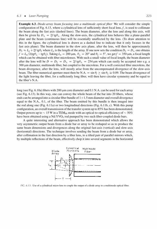
6.3 � Laser Pumping 223
Example 6.3. Diode-array beam focusing into a multimode optical fiber We will consider the simpleconfiguration of Fig. 6.13, where a cylindrical lens of sufficiently short focal lens, f , is used to collimatethe beam along the fast axis (dashed lines). The beam diameter, after the lens and along this axis, willthen be given by D? D 2f tg?. Along the slow-axis, the cylindrical lens behaves like a plane-parallelplate and the beam (continuous line) will be essentially unaffected by the lens. (To draw attention tothis in the figure, the cylindrical lens is drawn as a dashed line to indicate that it only focuses in thefast axis plane). The beam diameter in the slow axis plane, after the lens, will then be approximatelyDjj � La C2f tgjj where La is the length of the array. If one now sets the condition Djj D D? one obtainsf D La=2.tg? � tgjj/. Taking La D 200 μm, ? D 20ı and jj D 5ı, we get f D 350 μm, a focal lengthwhich can be obtained with fiber microlenses. With such a small value of focal length, the beam diameterafter the lens will be D D Djj D D? D 2f tg? D 254 μm which can easily be accepted into e.g. a300 μm diameter, multimode fiber, but coupled to the microlens. For a well corrected fiber microlens, thebeam divergence, after the lens, will mostly arise from the uncompensated divergence of the slow-axisbeam. The fiber numerical aperture must then be N.A. D sin f sin jj Š 0.09. The beam divergence ofthe light leaving the fiber, for a sufficiently long fiber, will then have circular symmetry and be equal tothe fiber’s N.A.
long (see Fig. 6.10a) fibers with 200 μm core diameter and 0.1 N.A. can be used for each array(see Fig. 6.13). In this way, one can convey the whole beam of the bar into 20 fibers, whoseends can be arranged into a circular fiber bundle of 1�1.5 mm diameter and overall divergenceequal to the N.A., 0.1, of the fiber. The beam emitted by this bundle is then imaged intothe rod along one (Fig. 6.11a) or two longitudinal directions (Fig. 6.11b, c). With this pumpconfiguration, an overall transmission of the transfer system up to 85% has been demonstrated.Output powers up to � 15 W in a TEM00 mode with an optical-to-optical efficiency of � 50%have been obtained using a Nd:YVO4 rod pumped by two such fiber-coupled diode bars.
A quite interesting and alternative approach has been demonstrated which allows thevery asymmetric output beam from a diode bar or array to be reshaped so as to produce thesame beam dimensions and divergences along the original fast-axis (vertical) and slow-axis(horizontal) directions. The technique involves sending the beam from a diode bar or array,after collimation in the fast direction by a fiber lens, to a tilted pair of parallel mirrors which,by multiple reflections of the beam, effectively chop it into several segments in the horizontal
FIG. 6.13. Use of a cylindrical micro-lens to couple the output of a diode array to a multimode optical fiber.
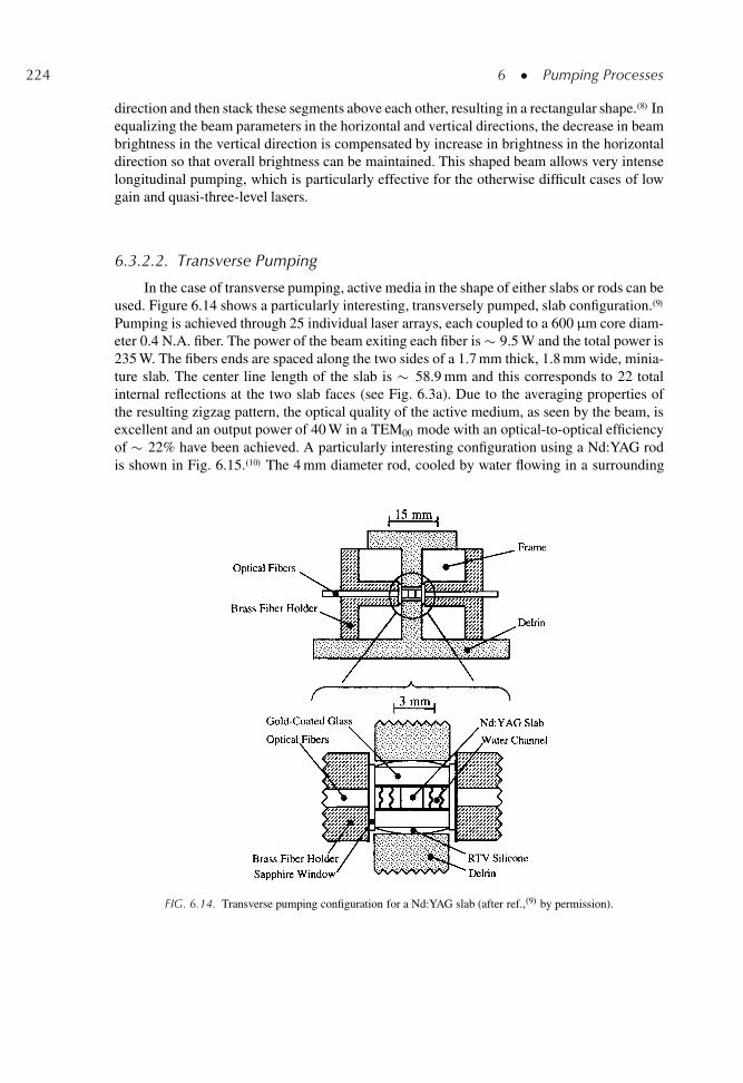
224 6 � Pumping Processes
direction and then stack these segments above each other, resulting in a rectangular shape..8/ Inequalizing the beam parameters in the horizontal and vertical directions, the decrease in beambrightness in the vertical direction is compensated by increase in brightness in the horizontaldirection so that overall brightness can be maintained. This shaped beam allows very intenselongitudinal pumping, which is particularly effective for the otherwise difficult cases of lowgain and quasi-three-level lasers.
6.3.2.2. Transverse Pumping
In the case of transverse pumping, active media in the shape of either slabs or rods can beused. Figure 6.14 shows a particularly interesting, transversely pumped, slab configuration..9/
Pumping is achieved through 25 individual laser arrays, each coupled to a 600 μm core diam-eter 0.4 N.A. fiber. The power of the beam exiting each fiber is � 9.5 W and the total power is235 W. The fibers ends are spaced along the two sides of a 1.7 mm thick, 1.8 mm wide, minia-ture slab. The center line length of the slab is � 58.9 mm and this corresponds to 22 totalinternal reflections at the two slab faces (see Fig. 6.3a). Due to the averaging properties ofthe resulting zigzag pattern, the optical quality of the active medium, as seen by the beam, isexcellent and an output power of 40 W in a TEM00 mode with an optical-to-optical efficiencyof � 22% have been achieved. A particularly interesting configuration using a Nd:YAG rodis shown in Fig. 6.15..10/ The 4 mm diameter rod, cooled by water flowing in a surrounding
FIG. 6.14. Transverse pumping configuration for a Nd:YAG slab (after ref.,.9/ by permission).
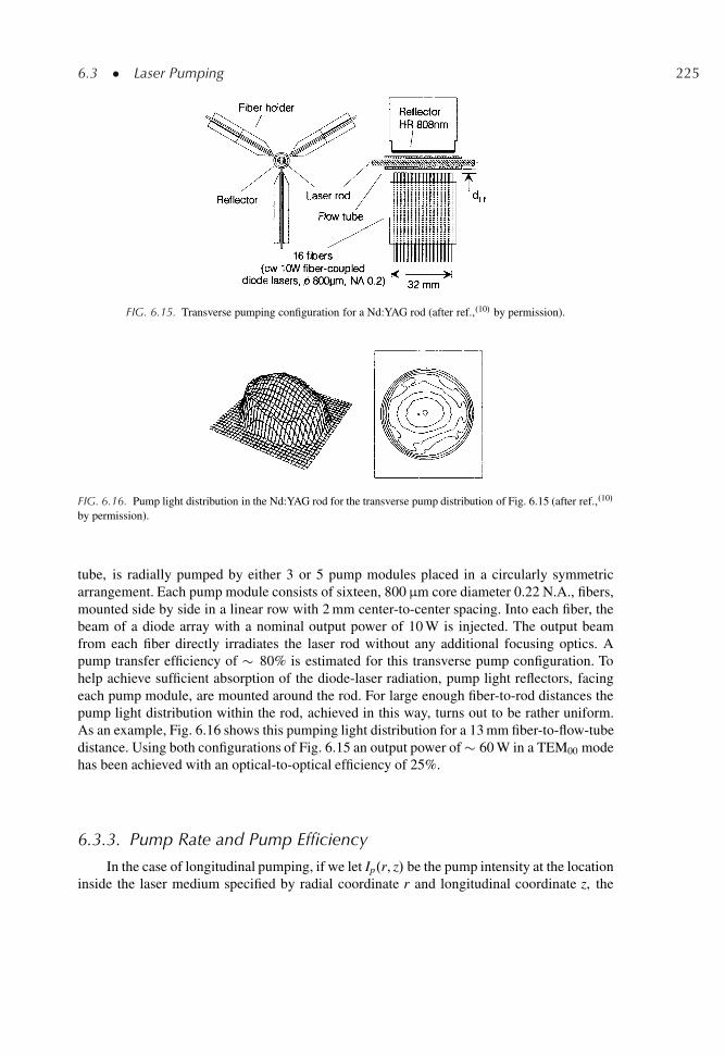
6.3 � Laser Pumping 225
FIG. 6.15. Transverse pumping configuration for a Nd:YAG rod (after ref.,.10/ by permission).
FIG. 6.16. Pump light distribution in the Nd:YAG rod for the transverse pump distribution of Fig. 6.15 (after ref.,.10/
by permission).
tube, is radially pumped by either 3 or 5 pump modules placed in a circularly symmetricarrangement. Each pump module consists of sixteen, 800 μm core diameter 0.22 N.A., fibers,mounted side by side in a linear row with 2 mm center-to-center spacing. Into each fiber, thebeam of a diode array with a nominal output power of 10 W is injected. The output beamfrom each fiber directly irradiates the laser rod without any additional focusing optics. Apump transfer efficiency of � 80% is estimated for this transverse pump configuration. Tohelp achieve sufficient absorption of the diode-laser radiation, pump light reflectors, facingeach pump module, are mounted around the rod. For large enough fiber-to-rod distances thepump light distribution within the rod, achieved in this way, turns out to be rather uniform.As an example, Fig. 6.16 shows this pumping light distribution for a 13 mm fiber-to-flow-tubedistance. Using both configurations of Fig. 6.15 an output power of � 60 W in a TEM00 modehas been achieved with an optical-to-optical efficiency of 25%.
6.3.3. Pump Rate and Pump Efficiency
In the case of longitudinal pumping, if we let Ip.r, z/ be the pump intensity at the locationinside the laser medium specified by radial coordinate r and longitudinal coordinate z, the
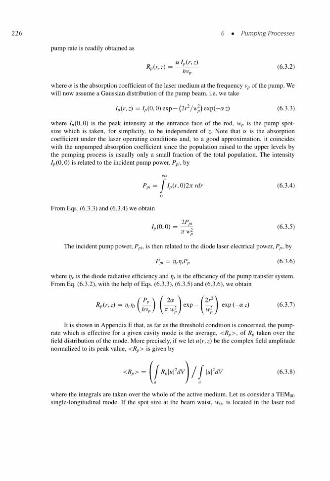
226 6 � Pumping Processes
pump rate is readily obtained as
Rp.r, z/ D ˛ Ip.r, z/
h�p(6.3.2)
where ˛ is the absorption coefficient of the laser medium at the frequency �p of the pump. Wewill now assume a Gaussian distribution of the pump beam, i.e. we take
Ip.r, z/ D Ip.0, 0/ exp � 2r2=w2p
�exp.�˛ z/ (6.3.3)
where Ip.0, 0/ is the peak intensity at the entrance face of the rod, wp is the pump spot-size which is taken, for simplicity, to be independent of z. Note that ˛ is the absorptioncoefficient under the laser operating conditions and, to a good approximation, it coincideswith the unpumped absorption coefficient since the population raised to the upper levels bythe pumping process is usually only a small fraction of the total population. The intensityIp.0, 0/ is related to the incident pump power, Ppi, by
Ppi D1Z
0
Ip.r, 0/2 rdr (6.3.4)
From Eqs. (6.3.3) and (6.3.4) we obtain
Ip.0, 0/ D 2Ppi
w2p
(6.3.5)
The incident pump power, Ppi, is then related to the diode laser electrical power, Pp, by
Ppi D �r�tPp (6.3.6)
where �r is the diode radiative efficiency and �t is the efficiency of the pump transfer system.From Eq. (6.3.2), with the help of Eqs. (6.3.3), (6.3.5) and (6.3.6), we obtain
Rp.r, z/ D �r�t
�Pp
h�p
� 2˛
w2p
!exp �
2r2
w2p
!exp .�˛ z/ (6.3.7)
It is shown in Appendix E that, as far as the threshold condition is concerned, the pump-rate which is effective for a given cavity mode is the average, <Rp>, of Rp taken over thefield distribution of the mode. More precisely, if we let u.r, z/ be the complex field amplitudenormalized to its peak value, <Rp> is given by
<Rp> D0@Z
a
Rpjuj2dV
1A.Z
a
juj2dV (6.3.8)
where the integrals are taken over the whole of the active medium. Let us consider a TEM00
single-longitudinal mode. If the spot size at the beam waist, w0, is located in the laser rod
6.3 � Laser Pumping 227
and if the spot size is assumed constant along the rod, then, according to Eq. (5.5.24), withR ! 1 and � Š 0, one has
juj2 / exp � 2r2=w20
�cos2 kz (6.3.9)
Equation (6.3.8) with the help of Eqs. (6.3.7) and (6.3.9) gives
<Rp> D �r�t
�Pp
h�p
�2 f1 � exp Œ�.˛l/�g w2
0 C w2p
�l
(6.3.10)
where l is the length of the laser rod. It should be noted that, in performing the integral alongthe z coordinate in Eq. (6.3.8), we have made the approximation
R l0 exp �.˛z/ cos2 kzdz Š
.1=2/R l
0 exp �.˛z/dz, using the fact that, since cos2.kz/ changes much more rapidly with zthen the exp �.˛z/ term, we can substitute cos2.kz/ with its average value < cos2.kz/> D.1=2/. If we now define the absorption efficiency, �a, as
�a D 1 � exp �.˛ l/ (6.3.11)
equation (6.3.10) can then be put in the more suggestive form
<Rp> D �p
�Pp
h�p
�2
w2
0 C w2p
�l
(6.3.12)
where we have defined �p D �r�t�a. Equation (6.3.12) constitutes the final result of ourcalculation for the effective pump rate in the case of longitudinal pumping. Note that, for agiven value of Pp, <Rp> increases as wp decreases so that the maximum value of<Rp>wouldbe attained for wp ! 0. For very small values of pump spot-size, however, divergence of thepump beam in the active rod cannot be neglected with the result that the beam may actuallybecome larger than the laser beam at the end of the rod. For this reason and to optimize theoptical efficiency, the condition wp Š w0 is often taken as a rough guide to the optimum case.
In the case of transverse pumping, we begin by writing the following obvious relationbetween pump rate and power, Ppi, incident on the rod
Za
h�p Rp dV D �a Ppi (6.3.13)
where �a is the fraction of the incident power which is absorbed in the active medium. Notethat, according to Eq. (6.3.11), the absorption efficiency �a can be written as �a Š .1 �exp �˛D/ where D is the relevant transverse dimension of the rod (D Š DR, where DR isthe rod diameter, for a single pass or D Š 2DR, for a double pass of the pump beam inthe rod). Equation (6.3.13) allows the pump rate to be calculated once its spatial variationis known. If we take, as a simple case, Rp D const, we obviously obtain from Eq. (6.3.13)Rp D �r�t�aPp=h�pAl where A is the cross-sectional area of the rod and where Eq. (6.3.6)has been used. To calculate <Rp> we consider a conceptually simpler model of the laser rod,where the active species is assumed to be confined to the central region of the rod, 0 r a,
228 6 � Pumping Processes
while the rod is undoped, for r > a (cladded rod). In this case, Eq. (6.3.9) can be taken tohold for any value of r while one has Rp D const for 0 r a and Rp D 0 for r > 0. Then,from Eqs. (6.3.8) and (6.3.9), we obtain
<Rp> D �p
�Pp
h�p
�Œ1 � exp � 2a2=w2
0
��
a2l(6.3.14)
where again we have written �p D �r�t�a. This equation constitutes the final result for ourcalculation of the effective pump rate in the case of transverse pumping.
For the comparison to be performed in sect. 6.3.5, it is appropriate to also calculatehere the effective pump rate that applies for lamp pumping. Assuming the cladded rod modelconsidered above and again taking Rp to be constant in the active medium, i.e., for 0 r a,we obtain from Eqs. (6.2.6) and (6.3.8)
<Rp> D �pl
�Pp
h�mp
�Œ1 � exp � 2a2=w2
0
��
a2l(6.3.15)
where �pl is the pumping efficiency for lamp pumping given, according to Eq. (6.2.5), by�pl D �r�t�a�pq.
6.3.4. Threshold Pump Power for Four-Leveland Quasi-Three-Level Lasers
With the results obtained in the previous section for the effective pump rate, we can nowgo on to calculate the expected threshold pump rate and threshold pump power for a givenlaser. We will limit our considerations to two very important cases: (i) An ideal four-levellaser, where pumped atoms are immediately transferred to the upper laser level, 2, and wherethe lower laser level, 1, is empty [see Fig. 1.4b]. (ii) An ideal quasi-three-level laser, wherepumped atoms are again transferred immediately to the upper laser level, 2, and where thelower laser level is a sublevel of the ground level 1. The first case includes lasers such asNd:YAG at � D 1.06 μm or � D 1.32 μm, Ti:Al2O3, and Cr:LISAF or LICAF. The mostimportant lasers belonging to the second category are Nd:YAG at � D 0.946 μm, Er:glass orYb:Er:glass at � Š 1.45 μm, Yb:YAG or Yb:glass, and Tm:Ho:YAG.
Let us first consider an ideal four-level laser and let us assume that the upper laser levelactually consists of many strongly coupled sublevels whose total combined population will becalled N2. According to Eq. (1.2.5), the threshold value of this population, N2c, can be writtenas N2c D �=�e l, where �e now indicates the effective stimulated emission cross-section [seesect. 2.7.2]. Actually, this previous expression only holds for a spatially uniform model i.e.,when both Rp and the mode configuration, juj2, are considered to be spatially independent.When spatial dependency is taken into account, the previous expression for the thresholdupper state population gets modified as follows (see Appendix E)
<N2>c D �=�e l (6.3.16)
6.3 � Laser Pumping 229
where <N2> is the effective value of population, given by
<N2> D0@Z
a
N2juj2dV
1A.Z
a
juj2dV (6.3.17)
The critical, or threshold, pump rate can then be obtained from the condition that thenumber of atoms raised by the pumping process must equal the number of atoms decayingspontaneously. Thus we get Rp D N2c=� , where � is the effective lifetime of the upper laserlevel, taking account of the decay of all the sublevels [see again sect. 2.7.2]. It then follows that
<Rp>c D <N2>c=� (6.3.18)
From Eqs. (6.3.16) and (6.3.18) we get
<Rp>c D �
�e l�(6.3.19)
Once the threshold value of the pump rate is calculated, we can readily obtain the corre-sponding threshold pump power. Using Eq. (6.3.19) into Eqs. (6.3.12) and (6.3.14), we get infact the following expressions
Pth D��
�p
� �h�p
�
� " w2
0 C w2p
�2�e
#(6.3.20)
Pth D��
�p
� �h�p
�
� ( a2
�e�1 � exp � 2a2=w2
0
�)
(6.3.21)
which hold for longitudinal and transverse pumping, respectively. The expression of thethreshold pump power for longitudinal pumping given by Eq. (6.3.20) agrees with that givenby Kubodera, Otsuka, and Miyazawa..19/ Note that, again for longitudinal pumping, thethreshold pump power increases as w0 is increased because, as w0 increases, the wings ofthe mode extend further into the less strongly pumped regions of the active medium. Like-wise, for transverse pumping and for the cladded rod model considered above, the thresholdpump power increases as w0 is increased because, as w0 increases, the wings of the modeextend further into the cladding, i.e., into the unpumped part of the medium. Similar consid-erations could be applied to the more realistic case of a rod without cladding. In this case,however, the calculation would be more involved because, in general, Eq. (6.3.9) would nolonger apply and the true field distribution, account being taken of the aperturing effects estab-lished by the finite rod diameter, would have to be used. When w0 is appreciably smaller thana (say w0 0.7a), however, the field distribution is not greatly affected by the presence ofthis aperture and Eq. (6.3.21) can be assumed to hold also for a rod without cladding. In thiscase, of course,
�1 � exp � 2a2=w2
0
�is very much closer to unity and, in calculating the
threshold pump power, this term could even be omitted from Eq. (6.3.21). As we will showin the next Chapter, however, it is important to keep this term in Eq. (6.3.21) to obtain thecorrect expression for the slope efficiency.
230 6 � Pumping Processes
For the comparison to be made in next section, it is also appropriate to calculate thethreshold pump rate for lamp pumping. From Eqs. (6.3.15) and (6.3.19) we get
Pth D��
�pl
� �h�mp
�
� ( a2
�e�1 � exp � 2a2=w2
0
�)
(6.3.22)
Let us now consider a quasi-three-level laser where the lower laser level, 1, is a sublevelof the ground level and assume that the population raised, from the pumping process, to thepump level(s) is immediately transferred to the upper laser level (ideal quasi-three-level laser).We will assume that all ground state sub-levels are strongly coupled and hence in thermalequilibrium and call N1 the total combined population of level 1. We will also assume that theupper laser level, level 2, consists of a number of strongly coupled sublevels and call N2
the total combined population of the upper level. The threshold values for the populationof the two levels is again established by the condition that the total net gain equals the losses.For the space-dependent case and according to Eq. (6.3.16) we now obtain (see Appendix E)
Œ�e<N2>c � �a<N1>c� l D � (6.3.23)
Where <N2> and <N1> again indicate spatially averaged values as in Eq. (6.3.17) and �e
and �a are, respectively, the effective values of the stimulated emission and absorption crosssections. Since, for an ideal quasi-three-level laser, one has N1 C N2 D Nt it follows that<N1> C <N2> D Nt and using this expression in Eq. (6.3.23) we can readily calculate<N2>c. The effective value of the threshold pump rate must again satisfy Eq. (6.3.18) and,using the value of <N2>c in this way calculated, we obtain
<Rp>c D Œ�aNt l C ��
.�e C �a/ l�(6.3.24)
Note that Eq. (6.3.24) obviously reduces to Eq. (6.3.19) if we let �a ! 0.In our calculation of the corresponding threshold pump power, we limit our considera-
tions to longitudinal pumping, since this is the only configuration which has allowed operationwith a reasonably low threshold, in this case. From Eqs. (6.3.24) and (6.3.12) we obtain
Pth D��aNt l C �
�p
� �h�p
�
� " w2
0 C w2p
�2.�e C �a/
#(6.3.25)
which agrees with the expression given by Fan and Byer..20/ Note again that Eq. (6.3.25)reduces to Eq. (6.3.20) if we let �a ! 0.
6.3.5. Comparison Between Diode-pumping and Lamp-pumping
Following the discussion presented in the previous sections, we are now ready to per-form a general comparison between lamp pumping and diode pumping. The comparison canonly be made for four-level lasers, since quasi-three-level lasers have mostly been operatedby means of longitudinal pumping by diodes. To compare Eq. (6.3.22) with Eqs. (6.3.20)
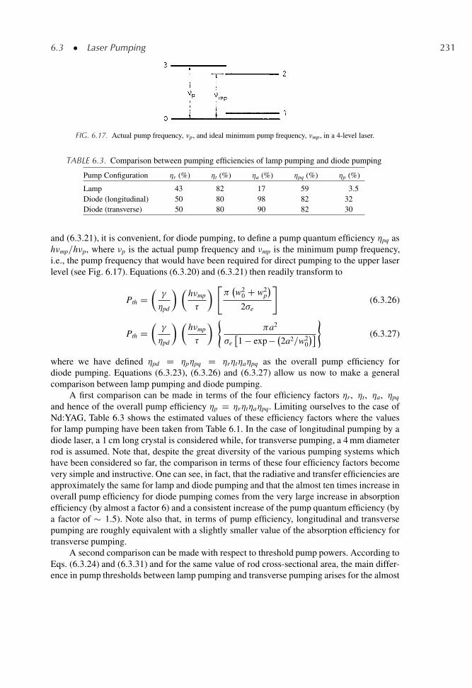
6.3 � Laser Pumping 231
FIG. 6.17. Actual pump frequency, �p, and ideal minimum pump frequency, �mp, in a 4-level laser.
TABLE 6.3. Comparison between pumping efficiencies of lamp pumping and diode pumping
Pump Configuration �r (%) �t (%) �a (%) �pq (%) �p (%)
Lamp 43 82 17 59 3.5Diode (longitudinal) 50 80 98 82 32Diode (transverse) 50 80 90 82 30
and (6.3.21), it is convenient, for diode pumping, to define a pump quantum efficiency �pq ash�mp=h�p, where �p is the actual pump frequency and �mp is the minimum pump frequency,i.e., the pump frequency that would have been required for direct pumping to the upper laserlevel (see Fig. 6.17). Equations (6.3.20) and (6.3.21) then readily transform to
Pth D��
�pd
� �h�mp
�
� " w2
0 C w2p
�2�e
#(6.3.26)
Pth D��
�pd
� �h�mp
�
� ( a2
�e�1 � exp � 2a2=w2
0
�)
(6.3.27)
where we have defined �pd D �p�pq D �r�t�a�pq as the overall pump efficiency fordiode pumping. Equations (6.3.23), (6.3.26) and (6.3.27) allow us now to make a generalcomparison between lamp pumping and diode pumping.
A first comparison can be made in terms of the four efficiency factors �r, �t, �a, �pq
and hence of the overall pump efficiency �p D �r�t�a�pq. Limiting ourselves to the case ofNd:YAG, Table 6.3 shows the estimated values of these efficiency factors where the valuesfor lamp pumping have been taken from Table 6.1. In the case of longitudinal pumping by adiode laser, a 1 cm long crystal is considered while, for transverse pumping, a 4 mm diameterrod is assumed. Note that, despite the great diversity of the various pumping systems whichhave been considered so far, the comparison in terms of these four efficiency factors becomevery simple and instructive. One can see, in fact, that the radiative and transfer efficiencies areapproximately the same for lamp and diode pumping and that the almost ten times increase inoverall pump efficiency for diode pumping comes from the very large increase in absorptionefficiency (by almost a factor 6) and a consistent increase of the pump quantum efficiency (bya factor of � 1.5). Note also that, in terms of pump efficiency, longitudinal and transversepumping are roughly equivalent with a slightly smaller value of the absorption efficiency fortransverse pumping.
A second comparison can be made with respect to threshold pump powers. According toEqs. (6.3.24) and (6.3.31) and for the same value of rod cross-sectional area, the main differ-ence in pump thresholds between lamp pumping and transverse pumping arises for the almost
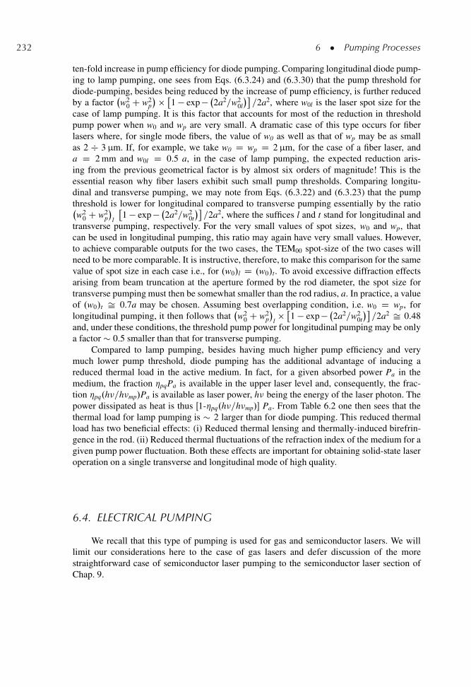
232 6 � Pumping Processes
ten-fold increase in pump efficiency for diode pumping. Comparing longitudinal diode pump-ing to lamp pumping, one sees from Eqs. (6.3.24) and (6.3.30) that the pump threshold fordiode-pumping, besides being reduced by the increase of pump efficiency, is further reducedby a factor
w2
0 C w2p
� � �1 � exp � 2a2=w2
0l
�=2a2, where w0l is the laser spot size for the
case of lamp pumping. It is this factor that accounts for most of the reduction in thresholdpump power when w0 and wp are very small. A dramatic case of this type occurs for fiberlasers where, for single mode fibers, the value of w0 as well as that of wp may be as smallas 2 � 3 μm. If, for example, we take w0 D wp D 2 μm, for the case of a fiber laser, anda D 2 mm and w0l D 0.5 a, in the case of lamp pumping, the expected reduction aris-ing from the previous geometrical factor is by almost six orders of magnitude! This is theessential reason why fiber lasers exhibit such small pump thresholds. Comparing longitu-dinal and transverse pumping, we may note from Eqs. (6.3.22) and (6.3.23) that the pumpthreshold is lower for longitudinal compared to transverse pumping essentially by the ratiow2
0 C w2p
�l
�1 � exp � 2a2=w2
0t
�=2a2, where the suffices l and t stand for longitudinal and
transverse pumping, respectively. For the very small values of spot sizes, w0 and wp, thatcan be used in longitudinal pumping, this ratio may again have very small values. However,to achieve comparable outputs for the two cases, the TEM00 spot-size of the two cases willneed to be more comparable. It is instructive, therefore, to make this comparison for the samevalue of spot size in each case i.e., for .w0/l D .w0/t. To avoid excessive diffraction effectsarising from beam truncation at the aperture formed by the rod diameter, the spot size fortransverse pumping must then be somewhat smaller than the rod radius, a. In practice, a valueof .w0/t Š 0.7a may be chosen. Assuming best overlapping condition, i.e. w0 D wp, forlongitudinal pumping, it then follows that
w2
0 C w2p
�l� �
1 � exp � 2a2=w20t
�=2a2 Š 0.48
and, under these conditions, the threshold pump power for longitudinal pumping may be onlya factor � 0.5 smaller than that for transverse pumping.
Compared to lamp pumping, besides having much higher pump efficiency and verymuch lower pump threshold, diode pumping has the additional advantage of inducing areduced thermal load in the active medium. In fact, for a given absorbed power Pa in themedium, the fraction �pqPa is available in the upper laser level and, consequently, the frac-tion �pq.h�=h�mp/Pa is available as laser power, h� being the energy of the laser photon. Thepower dissipated as heat is thus Œ1-�pq.h�=h�mp/� Pa. From Table 6.2 one then sees that thethermal load for lamp pumping is � 2 larger than for diode pumping. This reduced thermalload has two beneficial effects: (i) Reduced thermal lensing and thermally-induced birefrin-gence in the rod. (ii) Reduced thermal fluctuations of the refraction index of the medium for agiven pump power fluctuation. Both these effects are important for obtaining solid-state laseroperation on a single transverse and longitudinal mode of high quality.
6.4. ELECTRICAL PUMPING
We recall that this type of pumping is used for gas and semiconductor lasers. We willlimit our considerations here to the case of gas lasers and defer discussion of the morestraightforward case of semiconductor laser pumping to the semiconductor laser section ofChap. 9.
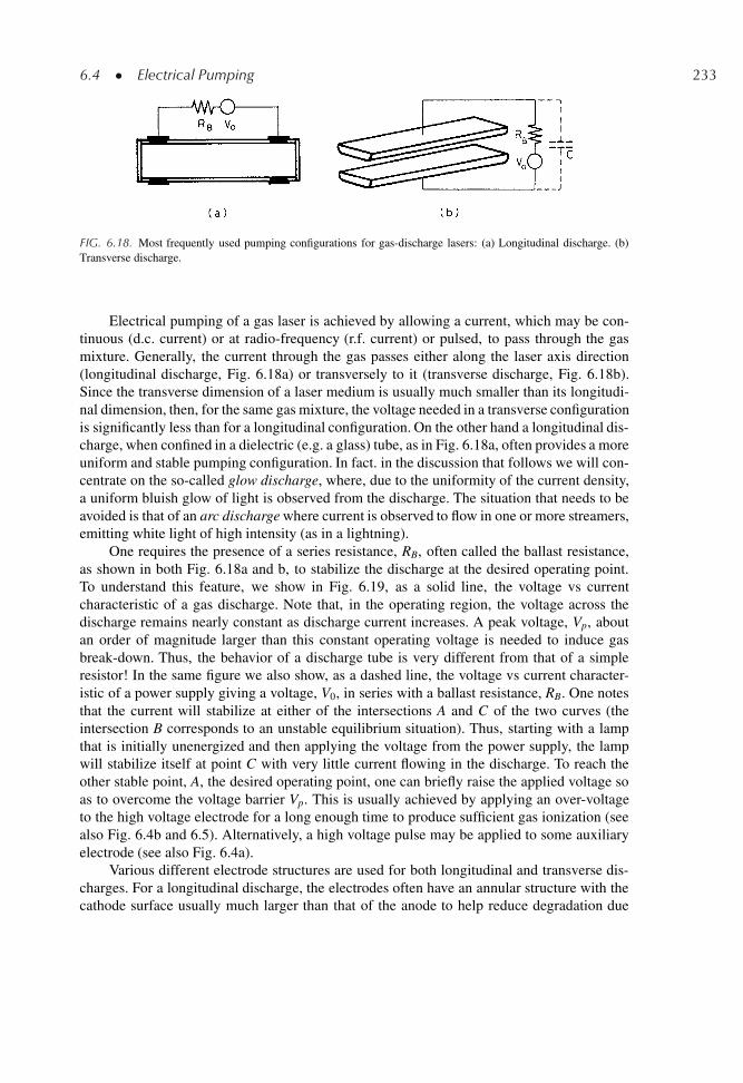
6.4 � Electrical Pumping 233
FIG. 6.18. Most frequently used pumping configurations for gas-discharge lasers: (a) Longitudinal discharge. (b)Transverse discharge.
Electrical pumping of a gas laser is achieved by allowing a current, which may be con-tinuous (d.c. current) or at radio-frequency (r.f. current) or pulsed, to pass through the gasmixture. Generally, the current through the gas passes either along the laser axis direction(longitudinal discharge, Fig. 6.18a) or transversely to it (transverse discharge, Fig. 6.18b).Since the transverse dimension of a laser medium is usually much smaller than its longitudi-nal dimension, then, for the same gas mixture, the voltage needed in a transverse configurationis significantly less than for a longitudinal configuration. On the other hand a longitudinal dis-charge, when confined in a dielectric (e.g. a glass) tube, as in Fig. 6.18a, often provides a moreuniform and stable pumping configuration. In fact. in the discussion that follows we will con-centrate on the so-called glow discharge, where, due to the uniformity of the current density,a uniform bluish glow of light is observed from the discharge. The situation that needs to beavoided is that of an arc discharge where current is observed to flow in one or more streamers,emitting white light of high intensity (as in a lightning).
One requires the presence of a series resistance, RB, often called the ballast resistance,as shown in both Fig. 6.18a and b, to stabilize the discharge at the desired operating point.To understand this feature, we show in Fig. 6.19, as a solid line, the voltage vs currentcharacteristic of a gas discharge. Note that, in the operating region, the voltage across thedischarge remains nearly constant as discharge current increases. A peak voltage, Vp, aboutan order of magnitude larger than this constant operating voltage is needed to induce gasbreak-down. Thus, the behavior of a discharge tube is very different from that of a simpleresistor! In the same figure we also show, as a dashed line, the voltage vs current character-istic of a power supply giving a voltage, V0, in series with a ballast resistance, RB. One notesthat the current will stabilize at either of the intersections A and C of the two curves (theintersection B corresponds to an unstable equilibrium situation). Thus, starting with a lampthat is initially unenergized and then applying the voltage from the power supply, the lampwill stabilize itself at point C with very little current flowing in the discharge. To reach theother stable point, A, the desired operating point, one can briefly raise the applied voltage soas to overcome the voltage barrier Vp. This is usually achieved by applying an over-voltageto the high voltage electrode for a long enough time to produce sufficient gas ionization (seealso Fig. 6.4b and 6.5). Alternatively, a high voltage pulse may be applied to some auxiliaryelectrode (see also Fig. 6.4a).
Various different electrode structures are used for both longitudinal and transverse dis-charges. For a longitudinal discharge, the electrodes often have an annular structure with thecathode surface usually much larger than that of the anode to help reduce degradation due
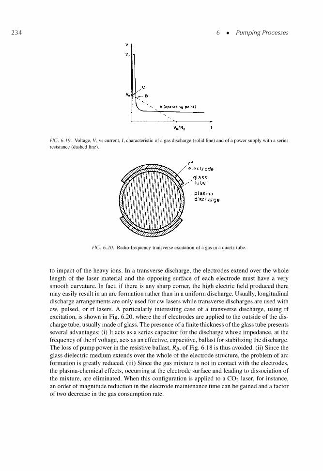
234 6 � Pumping Processes
FIG. 6.19. Voltage, V , vs current, I, characteristic of a gas discharge (solid line) and of a power supply with a seriesresistance (dashed line).
FIG. 6.20. Radio-frequency transverse excitation of a gas in a quartz tube.
to impact of the heavy ions. In a transverse discharge, the electrodes extend over the wholelength of the laser material and the opposing surface of each electrode must have a verysmooth curvature. In fact, if there is any sharp corner, the high electric field produced theremay easily result in an arc formation rather than in a uniform discharge. Usually, longitudinaldischarge arrangements are only used for cw lasers while transverse discharges are used withcw, pulsed, or rf lasers. A particularly interesting case of a transverse discharge, using rfexcitation, is shown in Fig. 6.20, where the rf electrodes are applied to the outside of the dis-charge tube, usually made of glass. The presence of a finite thickness of the glass tube presentsseveral advantages: (i) It acts as a series capacitor for the discharge whose impedance, at thefrequency of the rf voltage, acts as an effective, capacitive, ballast for stabilizing the discharge.The loss of pump power in the resistive ballast, RB, of Fig. 6.18 is thus avoided. (ii) Since theglass dielectric medium extends over the whole of the electrode structure, the problem of arcformation is greatly reduced. (iii) Since the gas mixture is not in contact with the electrodes,the plasma-chemical effects, occurring at the electrode surface and leading to dissociation ofthe mixture, are eliminated. When this configuration is applied to a CO2 laser, for instance,an order of magnitude reduction in the electrode maintenance time can be gained and a factorof two decrease in the gas consumption rate.
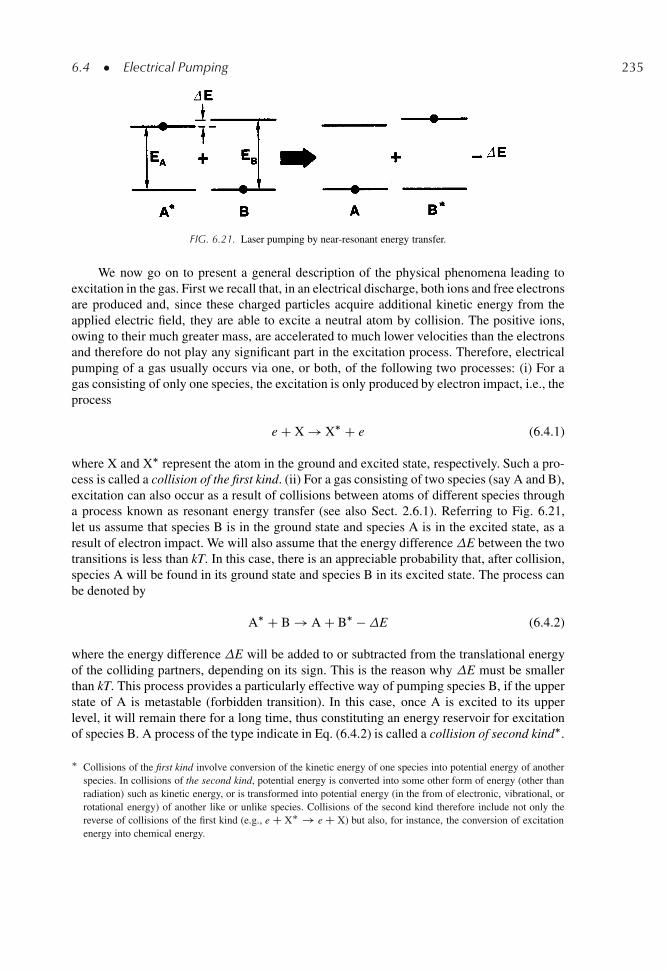
6.4 � Electrical Pumping 235
FIG. 6.21. Laser pumping by near-resonant energy transfer.
We now go on to present a general description of the physical phenomena leading toexcitation in the gas. First we recall that, in an electrical discharge, both ions and free electronsare produced and, since these charged particles acquire additional kinetic energy from theapplied electric field, they are able to excite a neutral atom by collision. The positive ions,owing to their much greater mass, are accelerated to much lower velocities than the electronsand therefore do not play any significant part in the excitation process. Therefore, electricalpumping of a gas usually occurs via one, or both, of the following two processes: (i) For agas consisting of only one species, the excitation is only produced by electron impact, i.e., theprocess
e C X ! X� C e (6.4.1)
where X and X� represent the atom in the ground and excited state, respectively. Such a pro-cess is called a collision of the first kind. (ii) For a gas consisting of two species (say A and B),excitation can also occur as a result of collisions between atoms of different species througha process known as resonant energy transfer (see also Sect. 2.6.1). Referring to Fig. 6.21,let us assume that species B is in the ground state and species A is in the excited state, as aresult of electron impact. We will also assume that the energy differenceE between the twotransitions is less than kT. In this case, there is an appreciable probability that, after collision,species A will be found in its ground state and species B in its excited state. The process canbe denoted by
A� C B ! A C B� �E (6.4.2)
where the energy difference E will be added to or subtracted from the translational energyof the colliding partners, depending on its sign. This is the reason why E must be smallerthan kT. This process provides a particularly effective way of pumping species B, if the upperstate of A is metastable (forbidden transition). In this case, once A is excited to its upperlevel, it will remain there for a long time, thus constituting an energy reservoir for excitationof species B. A process of the type indicate in Eq. (6.4.2) is called a collision of second kind�.
� Collisions of the first kind involve conversion of the kinetic energy of one species into potential energy of anotherspecies. In collisions of the second kind, potential energy is converted into some other form of energy (other thanradiation) such as kinetic energy, or is transformed into potential energy (in the from of electronic, vibrational, orrotational energy) of another like or unlike species. Collisions of the second kind therefore include not only thereverse of collisions of the first kind (e.g., e C X� ! e C X) but also, for instance, the conversion of excitationenergy into chemical energy.
236 6 � Pumping Processes
In the discussion that follows we will limit our considerations to just the electron impactexcitation process since it is both the most common and the simplest excitation mechanism.Also, electron impact excitation constitutes the first step for the near-resonant energy transferprocess.
6.4.1. Electron Impact Excitation
Electron impacts involve both elastic and inelastic collisions. In an inelastic collision, theatom may either be excited to a higher state or be ionized. Of the various possible excitationsthe one we are usually interested in is that which excites the atomic species to the desiredupper laser level. In order to describe the above excitation phenomena by means of appropri-ate collision cross-sections, we will first consider the simple case of impact excitation by acollimated beam of mono-energetic electrons. If Fe is the electron flux (number of electronsper unit area per unit time), a total cross section �e can be defined in a similar way to the caseof a photon flux [see Eq. (2.4.20)]. Thus, if we let dFe be the change of flux that results fromthe beam traveling a distance dz in the material, we can write
dFe D ��eNtFedz (6.4.3)
where Nt is the total population of the atomic species. Collisions that produce electronic exci-tation will only account for some fraction of the total cross section. In fact, the cross sectionfor elastic collisions, �el, is usually the largest, its order of magnitude being � 10�16 cm2. Ifwe now let �e2 be the cross section for electronic excitation from the ground level to the upperlaser level, then, according to Eq. (6.4.3), the rate of population of the upper state due to thepumping process is
.dN2=dt/p D �e2NtFe D NtNe��e2 (6.4.4)
where � is the electron velocity and Ne is the electron density. A calculation of the pump raterequires a knowledge of the value of �e2, which is expected to depend on the energy E of theincident electron, i.e. �e2 D �e2.E/. In a gas discharge the electrons have a distribution ofenergies which can be described by the distribution f .E/; its meaning is that dp D f .E/dErepresents the elemental probability that the electron energy ranges between E and E C dE.In this case the rate of population of the upper state is obtained from Eq. (6.4.4) by averagingover this distribution, viz.
.dN2=dt/p D NtNe<��e2> (6.4.5)
where
<��> DZ�� .E/f .E/dE (6.4.6)
According to Eqs. (1.3.1) and (6.4.5) the pump rate is then given by
Rp D NtNe<��e2> (6.4.7)
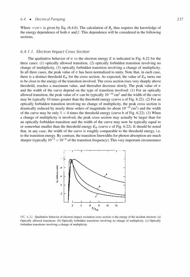
6.4 � Electrical Pumping 237
Where <��> is given by Eq. (6.4.6). The calculation of Rp thus requires the knowledge ofthe energy dependence of both � and f . This dependence will be considered in the followingsections.
6.4.1.1. Electron Impact Cross Section
The qualitative behavior of � vs the electron energy E is indicated in Fig. 6.22 for thethree cases: (1) optically allowed transition, (2) optically forbidden transition involving nochange of multiplicity, (3) optically forbidden transition involving a change of multiplicity.In all three cases, the peak value of � has been normalized to unity. Note that, in each case,there is a distinct threshold Eth for the cross section. As expected, the value of Eth turns outto be close to the energy of the transition involved. The cross section rises very sharply abovethreshold, reaches a maximum value, and thereafter decrease slowly. The peak value of �and the width of the curve depend on the type of transition involved: (1) For an opticallyallowed transition, the peak value of � can be typically 10�16 cm2 and the width of the curvemay be typically 10 times greater than the threshold energy (curve a of Fig. 6.22). (2) For anoptically forbidden transition involving no change of multiplicity, the peak cross section isdrastically reduced by nearly three orders of magnitude (to about 10�19 cm2) and the widthof the curve may be only 3 � 4 times the threshold energy (curve b of Fig. 6.22). (3) Whena change of multiplicity is involved, the peak cross section may actually be larger than foran optically forbidden transition and the width of the curve may now be typically equal toor somewhat smaller than the threshold energy Eth (curve c of Fig. 6.22). It should be notedthat, in any case, the width of the curve is roughly comparable to the threshold energy, i.e.to the transition energy. By contrast, the transition linewidths for photon absorption are muchsharper (typically 10�4 � 10�6 of the transition frequency). This very important circumstance
FIG. 6.22. Qualitative behavior of electron-impact excitation cross section vs the energy of the incident electron: (a)Optically allowed transitions. (b) Optically forbidden transitions involving no change of multiplicity. (c) Opticallyforbidden transitions involving a change of multiplicity.
238 6 � Pumping Processes
arises from the fact that, as explained in Sect. 6.1, the electron impact excitation is basicallya non-resonant phenomenon. This is the basic reason why excitation of a gaseous medium isperformed much more effectively by a “polychromatic” source of electrons (such as in a gasdischarge) than by a polychromatic light source (such as a lamp).
To provide a deeper insight into the mechanism involved in electron impact excitation,we now give a sketch of the procedure for a quantum mechanical calculation of the crosssection � . For optically allowed transitions or for optically forbidden transitions involving nochange of multiplicity, the simplest, and often the most accurate, calculation uses the Bornapproximation. Before collision, the atom is described by the ground state wave-function u1
and the incident electron by the plane wave function exp.jk0 � r/, where k0 is the electronwave vector and r is the vector describing the position of the incident electron with respect toa center situated e.g. at the nuclear position. After collision, the atom is described by the upperstate wave-function u2 and the scattered electron by the plane wave exp.jkn � r/, where kn isthe wave-vector of the scattered electron. For the discussion that follows, one needs to recallthat k D 2 =�, where � is the deBroglie wavelength of the electron which can be expressedas � D .1.23=
pV/ nm, where V is the electron energy in electron volts. The interaction
has its origin in the electrostatic repulsion between the incident electron and the electronsof the atom. This interaction is assumed to be weak enough for there be only a very smallprobability of a transition occurring in the atom during the impact and for the chance of twosuch transitions to be negligible. In this case the Schrodinger equation for the problem can belinearized. It then turns out that the transition rate and hence the transition cross section canbe expressed as
�e /ˇˇZŒu2 exp.jkn � r/��Œu1 exp.jk0 � r/� dV
ˇˇ2
(6.4.8)
From the above expression for the deBroglie wavelength and assuming an electronenergy of only a few eV, the wavelength �0 D 2 =jk0 � knj D 2 =j�kj is seen to be appre-ciably larger than the atomic dimensions. This means that .�k � r/ � 1 for jrj a, wherea is the atomic radius. In this case the factor exp jŒ.k0 � kn/ � r� D exp j.�k � r/ appearingin Eq. (6.4.8) can be expanded as a power series of .�k � r/. Since u1 and u2 are orthogonalfunctions, the first term in this expansion which gives a non-vanishing term for �e, is j.�k � r/and one gets
�e /ˇˇZ
u�2 ru1dV
ˇˇ2
/ jμ21j2 (6.4.9)
where μ21 is the matrix element of the electric dipole moment of the atom [see Eq. (2.3.7)].It then follows that, when μ21 ¤ 0, i.e. when the transition is optically allowed, the electronimpact cross section turns out to be proportional to the photon absorption cross section. Thusstrong optically allowed transitions are expected to also show a large cross section for electronimpact. For optically forbidden transitions involving no change of multiplicity (S D 0, e.g.the 11S ! 21S transition in He, see Chap. 10), Eq. (6.4.8) gives a non-vanishing value forthe next-higher-order term in the expansion of exp j.�k � r/ namely �.k � r/2=2. This means
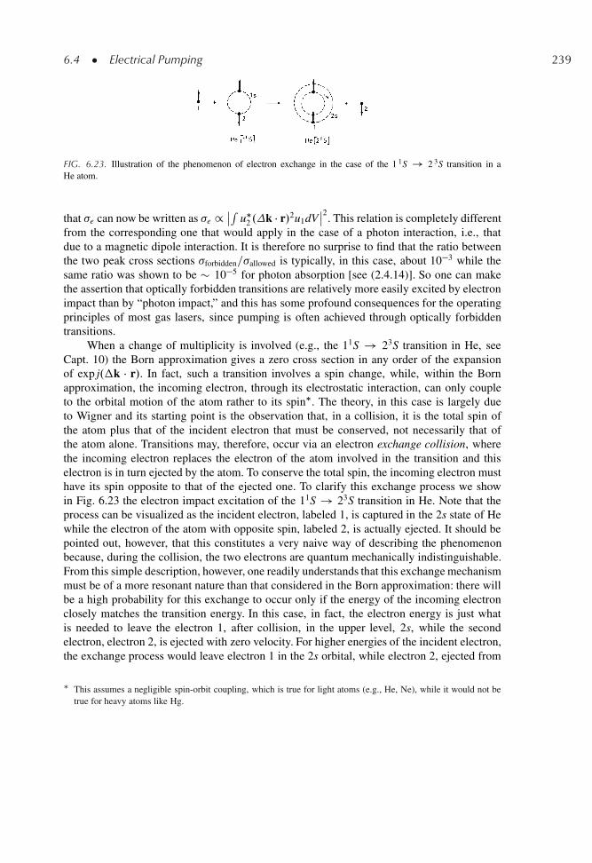
6.4 � Electrical Pumping 239
FIG. 6.23. Illustration of the phenomenon of electron exchange in the case of the 1 1S ! 2 3S transition in aHe atom.
that �e can now be written as �e / ˇRu�
2 .k � r/2u1dVˇ2
. This relation is completely differentfrom the corresponding one that would apply in the case of a photon interaction, i.e., thatdue to a magnetic dipole interaction. It is therefore no surprise to find that the ratio betweenthe two peak cross sections �forbidden=�allowed is typically, in this case, about 10�3 while thesame ratio was shown to be � 10�5 for photon absorption [see (2.4.14)]. So one can makethe assertion that optically forbidden transitions are relatively more easily excited by electronimpact than by “photon impact,” and this has some profound consequences for the operatingprinciples of most gas lasers, since pumping is often achieved through optically forbiddentransitions.
When a change of multiplicity is involved (e.g., the 11S ! 23S transition in He, seeCapt. 10) the Born approximation gives a zero cross section in any order of the expansionof exp j.�k � r/. In fact, such a transition involves a spin change, while, within the Bornapproximation, the incoming electron, through its electrostatic interaction, can only coupleto the orbital motion of the atom rather to its spin�. The theory, in this case is largely dueto Wigner and its starting point is the observation that, in a collision, it is the total spin ofthe atom plus that of the incident electron that must be conserved, not necessarily that ofthe atom alone. Transitions may, therefore, occur via an electron exchange collision, wherethe incoming electron replaces the electron of the atom involved in the transition and thiselectron is in turn ejected by the atom. To conserve the total spin, the incoming electron musthave its spin opposite to that of the ejected one. To clarify this exchange process we showin Fig. 6.23 the electron impact excitation of the 11S ! 23S transition in He. Note that theprocess can be visualized as the incident electron, labeled 1, is captured in the 2s state of Hewhile the electron of the atom with opposite spin, labeled 2, is actually ejected. It should bepointed out, however, that this constitutes a very naive way of describing the phenomenonbecause, during the collision, the two electrons are quantum mechanically indistinguishable.From this simple description, however, one readily understands that this exchange mechanismmust be of a more resonant nature than that considered in the Born approximation: there willbe a high probability for this exchange to occur only if the energy of the incoming electronclosely matches the transition energy. In this case, in fact, the electron energy is just whatis needed to leave the electron 1, after collision, in the upper level, 2s, while the secondelectron, electron 2, is ejected with zero velocity. For higher energies of the incident electron,the exchange process would leave electron 1 in the 2s orbital, while electron 2, ejected from
� This assumes a negligible spin-orbit coupling, which is true for light atoms (e.g., He, Ne), while it would not betrue for heavy atoms like Hg.
240 6 � Pumping Processes
the atom, would carry off the corresponding surplus energy. This would definitely be a lesslikely process to occur. Having established that this process is somewhat resonant, we cannow understand why the peak cross section, in this resonant case, can be even higher than foroptically forbidden transitions involving no change of spin.
6.4.2. Thermal and Drift Velocities
As already mentioned in previous sections, it is the electrons that are responsible forthe phenomena occurring in a gas discharge. They acquire energy from the applied electricfield and lose or exchange energy through three processes: (1) Inelastic collisions with theatoms, or molecules, of the gas mixture, which either raise the atom to one of its excitedstates or ionize it. These electron-impact excitation or ionization phenomena are perhaps themost important processes for laser pumping, hence the extended discussion in these sections.(2) Elastic collisions with the atoms. If we assume that the atoms are at rest before collision(the mean velocity for an atom is indeed much smaller than for an electron), the electronwill lose energy upon collision. It can be shown by a straightforward analysis of the elasticcollision process that, for random direction of the scattered electron, the electron loses, onaverage, a fraction 2.m=M/ of its energy, where m is the mass of electron and M is the massof the atom. Note that this loss is very small since m=M is small (e.g., m=M D 1.3 � 10�5 forAr atoms). (3) Electron-electron collisions. For a gas which is ionized to a moderate degree,the frequency of such collisions is usually high since both particles are charged and exertforces on one another over a considerable distance. Moreover, since both colliding particleshave the same mass, the energy exchange in the collision is considerable. As a result of thecollision phenomena mentioned above and as a consequence of the electrons being acceleratedby the electric field of the discharge, the electron “gas” in the plasma acquires a distribution ofvelocities. We can describe this by introducing the distribution f .�x, �y, �z/ with the meaningthat f .�x, �y, �z/d�xd�yd�z, gives the elemental probability that the electron is found withvelocity components in a range d�x, d�y, d�z, around �x, �y, �z. Given this distribution we candefine a thermal velocity �th so that
�2th D <�2> (6.4.10)
where the average is taken over the velocity distribution. Similarly, we can define a driftvelocity, �drift, as the average velocity along the field direction i.e.
�drift D <�z> (6.4.11)
where the z-axis is taken along the field direction and where, again, the average is taken overthe electron velocity distribution.
To make a rough calculation of both �th and �drift we make the simplifying assumptionthat, at each collision, some constant fraction ı of the kinetic energy of the electron is lost.A first equation can then be obtained from a power balance consideration: the average powerlost by the electron must equal the average power delivered to the electron by the external field.To proceed with this, we note that the average kinetic energy of the electron is mv2
th=2 while
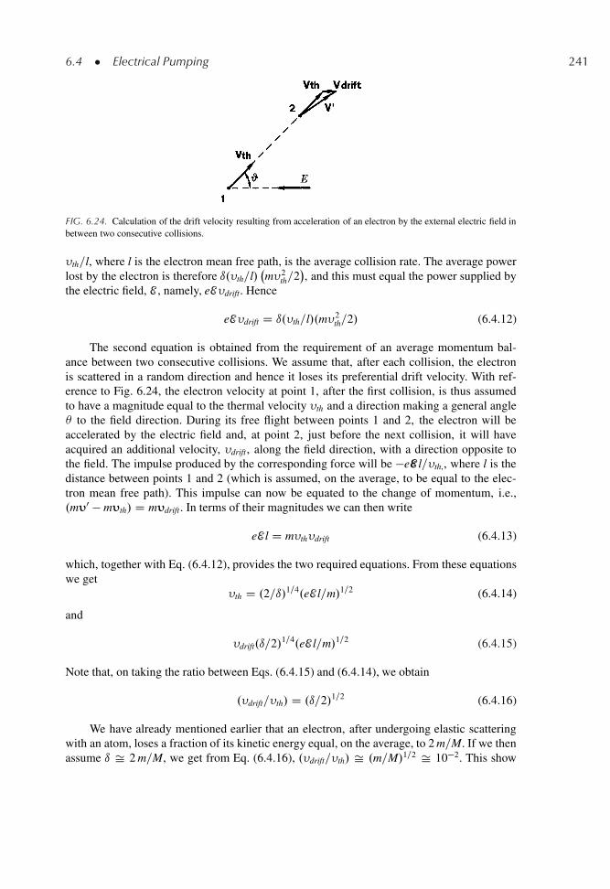
6.4 � Electrical Pumping 241
FIG. 6.24. Calculation of the drift velocity resulting from acceleration of an electron by the external electric field inbetween two consecutive collisions.
�th=l, where l is the electron mean free path, is the average collision rate. The average powerlost by the electron is therefore ı.�th=l/
m�2
th=2�, and this must equal the power supplied by
the electric field, E , namely, eE�drift. Hence
eE�drift D ı.�th=l/.m�2th=2/ (6.4.12)
The second equation is obtained from the requirement of an average momentum bal-ance between two consecutive collisions. We assume that, after each collision, the electronis scattered in a random direction and hence it loses its preferential drift velocity. With ref-erence to Fig. 6.24, the electron velocity at point 1, after the first collision, is thus assumedto have a magnitude equal to the thermal velocity �th and a direction making a general angle to the field direction. During its free flight between points 1 and 2, the electron will beaccelerated by the electric field and, at point 2, just before the next collision, it will haveacquired an additional velocity, �drift, along the field direction, with a direction opposite tothe field. The impulse produced by the corresponding force will be �eE l=�th,, where l is thedistance between points 1 and 2 (which is assumed, on the average, to be equal to the elec-tron mean free path). This impulse can now be equated to the change of momentum, i.e.,.mυ0 � mυth/ D mυdrift. In terms of their magnitudes we can then write
eE l D m�th�drift (6.4.13)
which, together with Eq. (6.4.12), provides the two required equations. From these equationswe get
�th D .2=ı/1=4.eE l=m/1=2 (6.4.14)
and
�drift.ı=2/1=4.eE l=m/1=2 (6.4.15)
Note that, on taking the ratio between Eqs. (6.4.15) and (6.4.14), we obtain
.�drift=�th/ D .ı=2/1=2 (6.4.16)
We have already mentioned earlier that an electron, after undergoing elastic scatteringwith an atom, loses a fraction of its kinetic energy equal, on the average, to 2 m=M. If we thenassume ı Š 2 m=M, we get from Eq. (6.4.16), .�drift=�th/ Š .m=M/1=2 Š 10�2. This show
242 6 � Pumping Processes
that the drift velocity is a very small fraction of the thermal velocity, so that we can considerthe movement of electrons in a gas as a slowly drifting swarm of randomly moving particlesrather than a stream of particles.
The calculation given above is a rather crude one since it is based on the assumptionthat the electron loses a constant fraction, ı, of its energy in each collision. Although this istrue for elastic collisions with atoms, this is not obviously true for inelastic collisions, wherethe energy lost equals the excitation energy of the atom. It should be noted that, althoughelastic collisions are actually more frequent than inelastic collisions, the energy lost in anelastic collision is, however, very small. Thus, if elastic collisions are the dominant process,the discharge would not provide a particularly efficient means for pumping a laser. Indeed, ifelastic collisions were the predominant mechanism of electron cooling, most of the dischargeenergy would be used to heat up rather than to excite the atoms. It should also be noted thatelectron-electron collision does not play any role in the energy balance equation expressed byEq. (6.4.12), since this process simply redistributes the electron velocities without changingtheir average energy.
6.4.3. Electron Energy Distribution
We now proceed to a consideration of the distribution of electron velocities or of electronenergies in a gas discharge. If the energy redistribution due to electron-electron collisions isfast enough compared to the energy loss due to both elastic and inelastic collision with theatoms, then the prediction of statistical mechanics is that the distribution of electron veloc-ities (or energies) is given by the Maxwell-Boltzmann (MB) distribution function. This canbe described, for instance, by the energy distribution function f .E/, where f .E/dE is the ele-mental probability for an electron to have its kinetic energy lying between E and E C dE. Wethen obtain
f .E/ D�
2
1=2kTe
� �E
kTe
�1=2
exp �.E=kTe/ (6.4.17)
where Te is the electron temperature. One thus sees that, when the distribution can bedescribed by the MB law, the electron temperature is the only parameter that needs to bespecified for characterizing the distribution.
Once Te is known, one can calculate �th from Eq. (4.10) using the electron energy distri-bution given by Eq. (6.4.17). Using the standard relation �2 D 2E=m, we readily obtain fromEq. (6.4.10)
�th D Œ3kTe=m�1=2 (6.4.18)
which relates �th to Te. From Eqs. (6.4.18) and (6.4.14) we then obtain
Te D"�
2
ı
�1=2 e
3k
#.E l/ (6.4.19)
Since the electron mean free path l is inversely proportional to the gas pressure p,Eq. (6.4.19) shows that, for a given gas mixture, Te is proportional to the ratio E=p. A more
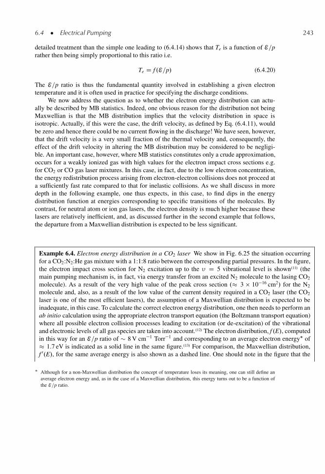
6.4 � Electrical Pumping 243
detailed treatment than the simple one leading to (6.4.14) shows that Te is a function of E=prather then being simply proportional to this ratio i.e.
Te D f .E=p/ (6.4.20)
The E=p ratio is thus the fundamental quantity involved in establishing a given electrontemperature and it is often used in practice for specifying the discharge conditions.
We now address the question as to whether the electron energy distribution can actu-ally be described by MB statistics. Indeed, one obvious reason for the distribution not beingMaxwellian is that the MB distribution implies that the velocity distribution in space isisotropic. Actually, if this were the case, the drift velocity, as defined by Eq. (6.4.11), wouldbe zero and hence there could be no current flowing in the discharge! We have seen, however,that the drift velocity is a very small fraction of the thermal velocity and, consequently, theeffect of the drift velocity in altering the MB distribution may be considered to be negligi-ble. An important case, however, where MB statistics constitutes only a crude approximation,occurs for a weakly ionized gas with high values for the electron impact cross sections e.g.for CO2 or CO gas laser mixtures. In this case, in fact, due to the low electron concentration,the energy redistribution process arising from electron-electron collisions does not proceed ata sufficiently fast rate compared to that for inelastic collisions. As we shall discuss in moredepth in the following example, one thus expects, in this case, to find dips in the energydistribution function at energies corresponding to specific transitions of the molecules. Bycontrast, for neutral atom or ion gas lasers, the electron density is much higher because theselasers are relatively inefficient, and, as discussed further in the second example that follows,the departure from a Maxwellian distribution is expected to be less significant.
Example 6.4. Electron energy distribution in a CO2 laser We show in Fig. 6.25 the situation occurringfor a CO2:N2:He gas mixture with a 1:1:8 ratio between the corresponding partial pressures. In the figure,the electron impact cross section for N2 excitation up to the � D 5 vibrational level is shown.11/ (themain pumping mechanism is, in fact, via energy transfer from an excited N2 molecule to the lasing CO2
molecule). As a result of the very high value of the peak cross section .� 3 � 10�16 cm2/ for the N2
molecule and, also, as a result of the low value of the current density required in a CO2 laser (the CO2
laser is one of the most efficient lasers), the assumption of a Maxwellian distribution is expected to beinadequate, in this case. To calculate the correct electron energy distribution, one then needs to perform anab initio calculation using the appropriate electron transport equation (the Boltzmann transport equation)where all possible electron collision processes leading to excitation (or de-excitation) of the vibrationaland electronic levels of all gas species are taken into account..12/ The electron distribution, f .E/, computedin this way for an E=p ratio of � 8 V cm�1 Torr�1 and corresponding to an average electron energy� of� 1.7 eV is indicated as a solid line in the same figure..13/ For comparison, the Maxwellian distribution,f 0.E/, for the same average energy is also shown as a dashed line. One should note in the figure that the
� Although for a non-Maxwellian distribution the concept of temperature loses its meaning, one can still define anaverage electron energy and, as in the case of a Maxwellian distribution, this energy turns out to be a function ofthe E=p ratio.
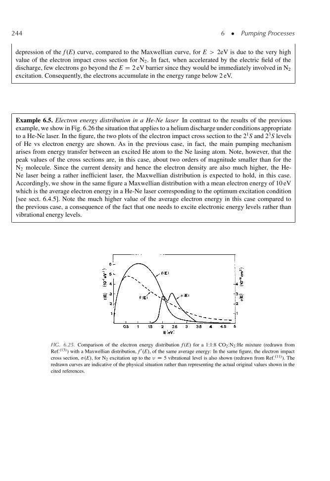
244 6 � Pumping Processes
depression of the f .E/ curve, compared to the Maxwellian curve, for E > 2eV is due to the very highvalue of the electron impact cross section for N2. In fact, when accelerated by the electric field of thedischarge, few electrons go beyond the E D 2 eV barrier since they would be immediately involved in N2
excitation. Consequently, the electrons accumulate in the energy range below 2 eV.
Example 6.5. Electron energy distribution in a He-Ne laser In contrast to the results of the previousexample, we show in Fig. 6.26 the situation that applies to a helium discharge under conditions appropriateto a He-Ne laser. In the figure, the two plots of the electron impact cross section to the 21S and 23S levelsof He vs electron energy are shown. As in the previous case, in fact, the main pumping mechanismarises from energy transfer between an excited He atom to the Ne lasing atom. Note, however, that thepeak values of the cross sections are, in this case, about two orders of magnitude smaller than for theN2 molecule. Since the current density and hence the electron density are also much higher, the He-Ne laser being a rather inefficient laser, the Maxwellian distribution is expected to hold, in this case.Accordingly, we show in the same figure a Maxwellian distribution with a mean electron energy of 10 eVwhich is the average electron energy in a He-Ne laser corresponding to the optimum excitation condition[see sect. 6.4.5]. Note the much higher value of the average electron energy in this case compared tothe previous case, a consequence of the fact that one needs to excite electronic energy levels rather thanvibrational energy levels.
FIG. 6.25. Comparison of the electron energy distribution f .E/ for a 1:1:8 CO2:N2:He mixture (redrawn fromRef..13/) with a Maxwellian distribution, f 0.E/, of the same average energy: In the same figure, the electron impactcross section, �.E/, for N2 excitation up to the � D 5 vibrational level is also shown (redrawn from Ref..11/). Theredrawn curves are indicative of the physical situation rather than representing the actual original values shown in thecited references.
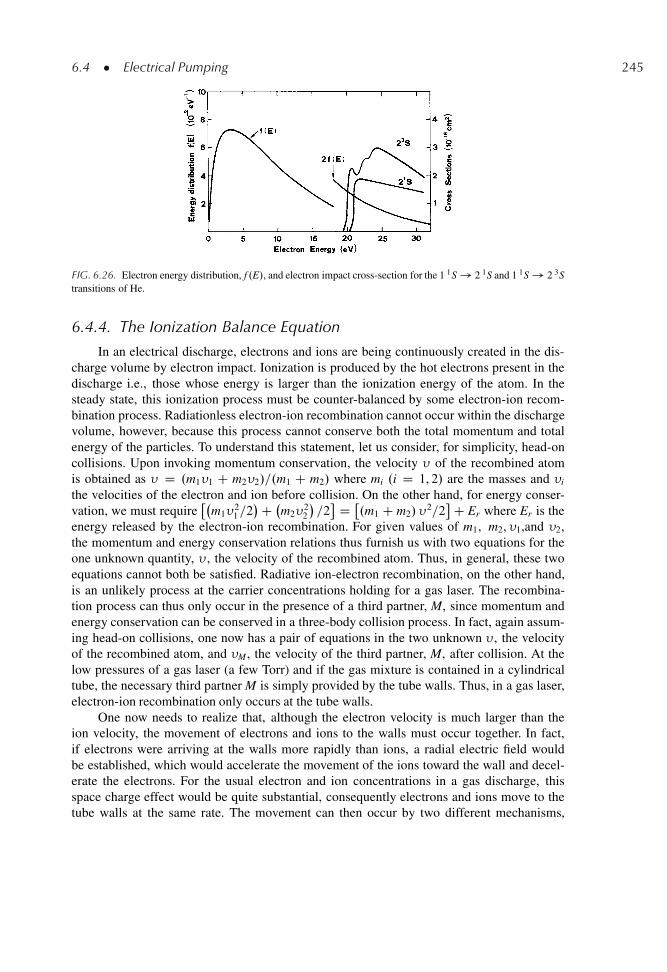
6.4 � Electrical Pumping 245
FIG. 6.26. Electron energy distribution, f .E/, and electron impact cross-section for the 1 1S ! 2 1S and 1 1S ! 2 3Stransitions of He.
6.4.4. The Ionization Balance Equation
In an electrical discharge, electrons and ions are being continuously created in the dis-charge volume by electron impact. Ionization is produced by the hot electrons present in thedischarge i.e., those whose energy is larger than the ionization energy of the atom. In thesteady state, this ionization process must be counter-balanced by some electron-ion recom-bination process. Radiationless electron-ion recombination cannot occur within the dischargevolume, however, because this process cannot conserve both the total momentum and totalenergy of the particles. To understand this statement, let us consider, for simplicity, head-oncollisions. Upon invoking momentum conservation, the velocity � of the recombined atomis obtained as � D .m1�1 C m2�2/=.m1 C m2/ where mi .i D 1, 2/ are the masses and �i
the velocities of the electron and ion before collision. On the other hand, for energy conser-vation, we must require
�m1�
21=2
�C m2�
22
�=2 D �
.m1 C m2/ �2=2
C Er where Er is theenergy released by the electron-ion recombination. For given values of m1, m2, �1,and �2,the momentum and energy conservation relations thus furnish us with two equations for theone unknown quantity, � , the velocity of the recombined atom. Thus, in general, these twoequations cannot both be satisfied. Radiative ion-electron recombination, on the other hand,is an unlikely process at the carrier concentrations holding for a gas laser. The recombina-tion process can thus only occur in the presence of a third partner, M, since momentum andenergy conservation can be conserved in a three-body collision process. In fact, again assum-ing head-on collisions, one now has a pair of equations in the two unknown � , the velocityof the recombined atom, and �M , the velocity of the third partner, M, after collision. At thelow pressures of a gas laser (a few Torr) and if the gas mixture is contained in a cylindricaltube, the necessary third partner M is simply provided by the tube walls. Thus, in a gas laser,electron-ion recombination only occurs at the tube walls.
One now needs to realize that, although the electron velocity is much larger than theion velocity, the movement of electrons and ions to the walls must occur together. In fact,if electrons were arriving at the walls more rapidly than ions, a radial electric field wouldbe established, which would accelerate the movement of the ions toward the wall and decel-erate the electrons. For the usual electron and ion concentrations in a gas discharge, thisspace charge effect would be quite substantial, consequently electrons and ions move to thetube walls at the same rate. The movement can then occur by two different mechanisms,
246 6 � Pumping Processes
Example 6.6. Thermal and drift velocities in He-Ne andCO2 lasers Based on what has been said in the pre-vious example, we will assume for a He-Ne laser anaverage electron energy <E> Š 10 eV. This meansthat
m�2
th=2� D <E> D 10 eV and therefore �th Š
1.9 � 106 m=s. Since the electron velocity distribution isassumed, in this case, to be Maxwellian, then, accordingto Eq. (6.4.18), the electron temperature can be obtainedfrom the relation Te D 2<E>=3k. We obtain Te Š7.7 � 104 K. Note the much higher value of the electrontemperature compared to room temperature. To calculatethe drift velocity, we make use of Eq. (6.4.16) and assumethat the dominant cooling process for the electrons is viaelastic collisions with the lighter He atoms. We then get.�drift=�th/ � .m=MHe/
1=2 Š 1.16 � 10�2, where MHe isthe mass of the Helium, so that �drift Š 2.2 � 104 m=s.In the case of a CO2 laser, based on the findings of exam-ple 6.4, we will assume an optimum electron energy valueof <E> Š 1.7 eV. From the relation
m�2
th=2� D <E>
we then get �th Š 0.78 � 106 m=s. The drift velocity canthen be obtained from ref..13/ assuming an E=p ratio of� 8 V cm�1 Torr�1 and a 1:1:8 partial pressure ratio ofthe CO2:N2:He mixture. We get �drift Š 6 � 104 m=s.Note that, in this case, we cannot talk about an electrontemperature since the electron energy distribution departsconsiderably from a Maxwellian distribution. Note alsothat, in both cases, the thermal velocity is � 106 m=s andthe drift velocity is � 100 times smaller.
depending on the gas pressure p and tuberadius R. If the ion mean free path ismuch shorter than R, electrons and ions dif-fuse together to the walls and recombinationoccurs by ambipolar diffusion. If the ionmean free path becomes comparable to thetube radius (as happens in the relatively low-pressure ion gas lasers), electrons and ionsreach the wall by “free flight” rather than bydiffusion. The analytical theory of ambipolardiffusion can be obtained.14/ from the Schot-tky theory of a discharge in the so calledpositive column. In the low pressure limit, onthe other hand, the free fall model of Tonks-Langmuir for the plasma discharge should beused..15/ The two theories are rather compli-cated and their description goes beyond thescope of this book. In both theories, however,a balance equation must always hold betweenthe number of electron-ion pairs producedand the number of electron-ion pairs recom-bining at the walls (ionization balance equa-tion). So, in the case of Schottky theory,the balance equation can be written, in ournotations, as
<��i>Ng D kTe
e�C
�2.405
R
�2
(6.4.21)
where �i is the ionization cross section, �C isthe ion mobility and R is the tube radius. One can now see that, for a given atomic species i.e.,with a given expression for �i D �i.E/, the average value <v�i> appearing in Eq. (6.4.21)will only depend on the electron temperature, Te. Ionization is in fact produced by the mostenergetic electrons in the energy distribution and their number depends on the temperature Te.One can also see that Ng is proportional to the gas pressure while the ion mobility is inverselyproportional to it. Equation (6.4.21) can then be rearranged as
f .Te/ D C=.pR/2 (6.4.22)
where we have written <��i>=kTe D f .Te/ and where C is a suitable constant. Thus, fora given atomic species, the ionization balance equation leads to a relation between Te andpR in much the same way as the energy and momentum balance equation leads to a relationbetween Te and E=p [see (6.4.20)]. The functional relation f D f .Te/ in Eq. (6.4.22) is suchthat Te increases as pR decreases. In fact, if for a given tube radius one decreases the gaspressure, the electron-ion recombination due to diffusion to the walls increases. The electron
6.4 � Electrical Pumping 247
temperature has therefore to increase in order to maintain the balance between ionization andrecombination. In the case of Tonks-Langmuir theory a similar functional relation again existsbetween Te and the pR product.
6.4.5. Scaling Laws for Electrical Discharge Lasers
Equations (6.4.20) and (6.4.22) provide two fundamental relations which can be used tounderstand a number of aspects of the physical behavior of any gas discharge. For example,we can now explain why, in a stable glow discharge, the voltage across a discharge tube isessentially independent of the current which is flowing (see Fig. 6.19). In fact, if we considersome given gas tube i.e. with given values of tube radius and gas pressure, then, according toEq. (6.4.22), the electron temperature is fixed. We then see from Eq. (6.4.20) that the electricfield must also be fixed and thus independent of the discharge current.
Let us now see the consequences of Eqs. (6.4.20) and (6.4.22) for a gas laser discharge.First we should note that, for a given gas medium, an optimum value of electron temperature,Topt, exists if we want to maximize the pump rate to the upper laser level. Too low a valuesof the electron temperature, in fact, would result in insufficient electron energy to excite theupper laser level. The electron energy will then be lost mostly through excitation of lowerlevels of the medium, including the lower laser level. Too high a value of the electron temper-ature, on the other hand, would lead to strong excitation of higher levels of the gas mixture(which may not be coupled to the upper laser level) or might produce excessive ionization ofthe gas mixture (which could result in a discharge instability, i.e., a transition from a glowdischarge to an arc). If we then set Te D Topt on the left hand side of both Eqs. (6.4.20)and (6.4.22), we obtain
.E=p/ D .E=p/opt (6.4.23a)
.pD/ D .pD/opt (6.4.23b)
Thus, for a given gas mixture, some optimum values exist for both pD and E=p if the mix-ture is to be used as the active medium of a gas laser. Equations (6.4.23) establish the scalinglaws for any gas laser. As an example of applying these laws, let us assume that we start withthe best operating conditions and that, for some reason, we want to decrease the tube diameterby e.g. a factor 2. Then, Eq. (6.4.23b) shows that we must increase the pressure of the gasmixture by the same factor if we want the laser to be still operating with optimum efficiency.If the pressure is doubled, then, according to Eq. (6.4.23a) the electric field, E , in the gasdischarge and hence the total voltage, V , across the laser tube, must also double. This meansthat the V versus I characteristic of the given laser tube (see solid line of Fig. 6.19) will scaleup by a factor 2 in voltage, at any given current. The open circuit voltage of the power supply,V0, and the ballast resistance, RB, must then be designed so as to have the desired currentflowing in the discharge tube.
248 6 � Pumping Processes
6.4.6. Pump Rate and Pump Efficiency
To calculate the pump rate, we first recall the standard equation J D e�driftNe whichrelates the current density, J, to the electron density, Ne, of a discharge. From Eq. (6.4.7) wethen obtain
Rp D NtJ
e
�<��>
�drift
�(6.4.24)
If a Maxwellian electron energy distribution is taken, the term <��> in Eq. (6.4.24)will depend only on the electron temperature, Te. According to Eqs. (6.4.15) and (6.4.19) onereadily sees that �drift also depends only on Te. For given values of the gas pressure, p, and tuberadius, R, the electron temperature remains constant, ideally at the optimum operating value. Itthen follows that the term in the square brackets of Eq. (6.4.24) is a constant, i.e. independentof the current density and one sees that Rp, in this simple model, increases linearly with thecurrent density. Just as for optical pumping we can now define a pumping efficiency, �p, as theratio between the minimum pump power which would ideally be needed to achieve a givenpump rate, Rp, and the actual electrical pump power, Pp, to the discharge. We thus write
�p D RpVah�mp
Pp(6.4.25)
where Va is the volume of the active medium and �mp is the frequency difference between theground level and the upper laser level. Note that, to a first approximation, �p can be taken tobe independent of the discharge current density since both Rp and Pp are proportional to J.
It should be noted that the expression for Rp given by Eq. (6.4.24) can only be taken as aqualitative guide to the complex phenomena occurring in gas laser pumping rather than as anaccurate quantitative expression for the actual value of the pump rate. As already mentionedearlier, particularly for the most efficient gas lasers, the electron energy distribution is sig-nificantly different from a Maxwell-Boltzmann distribution and its calculation requires an abinitio treatment of the Boltzmann transport equation with knowledge of all possible electroncollision processes leading to excitation (or de-excitation) of the rotational, vibrational, andelectronic levels of all the gas species present in the discharge. Furthermore, the number ofgas species may be much larger than the number of species initially introduced into the tube.For instance, for a CO2:N2:He mixture, various amounts are also found, in the discharge, ofCO, O2, N2O etc. depending on the complicated plasma-chemical reactions occurring in thevolume of the gas and at the electrodes. The calculation therefore gets quite involved, requir-ing the use of a computer and sometimes proving impractical due to lack of appropriate dataon electron collision cross sections for all of the components in the gas mixture..12/ Detailedcomputer calculation have therefore only been performed for gas mixtures of particular impor-tance such as the CO2:N2:He mixture used in high power CO2 lasers. One (apparent) way tocircumvent the problem is to assume that �p is known or that it can be estimated. In this casewe obviously obtain from Eq. (6.4.25)
Rp D �pPp
Alh�mp(6.4.26)
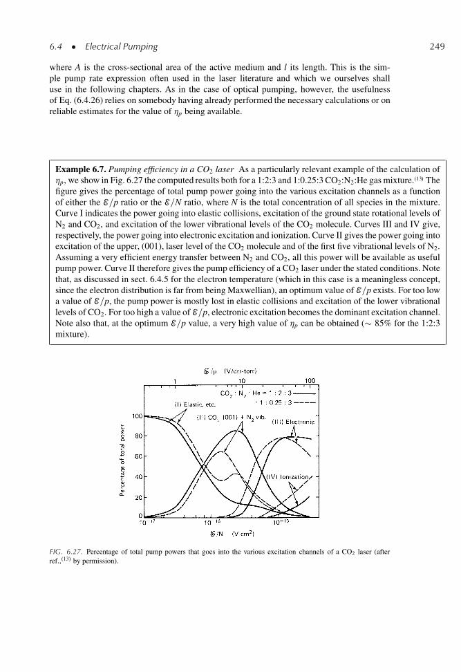
6.4 � Electrical Pumping 249
where A is the cross-sectional area of the active medium and l its length. This is the sim-ple pump rate expression often used in the laser literature and which we ourselves shalluse in the following chapters. As in the case of optical pumping, however, the usefulnessof Eq. (6.4.26) relies on somebody having already performed the necessary calculations or onreliable estimates for the value of �p being available.
Example 6.7. Pumping efficiency in a CO2 laser As a particularly relevant example of the calculation of�p, we show in Fig. 6.27 the computed results both for a 1:2:3 and 1:0.25:3 CO2:N2:He gas mixture..13/ Thefigure gives the percentage of total pump power going into the various excitation channels as a functionof either the E=p ratio or the E=N ratio, where N is the total concentration of all species in the mixture.Curve I indicates the power going into elastic collisions, excitation of the ground state rotational levels ofN2 and CO2, and excitation of the lower vibrational levels of the CO2 molecule. Curves III and IV give,respectively, the power going into electronic excitation and ionization. Curve II gives the power going intoexcitation of the upper, (001), laser level of the CO2 molecule and of the first five vibrational levels of N2.Assuming a very efficient energy transfer between N2 and CO2, all this power will be available as usefulpump power. Curve II therefore gives the pump efficiency of a CO2 laser under the stated conditions. Notethat, as discussed in sect. 6.4.5 for the electron temperature (which in this case is a meaningless concept,since the electron distribution is far from being Maxwellian), an optimum value of E=p exists. For too lowa value of E=p, the pump power is mostly lost in elastic collisions and excitation of the lower vibrationallevels of CO2. For too high a value of E=p, electronic excitation becomes the dominant excitation channel.Note also that, at the optimum E=p value, a very high value of �p can be obtained (� 85% for the 1:2:3mixture).
FIG. 6.27. Percentage of total pump powers that goes into the various excitation channels of a CO2 laser (afterref.,.13/ by permission).
250 6 � Pumping Processes
6.5. CONCLUSIONS
In this chapter optical pumping and electrical pumping have been considered in par-ticular detail. We have seen that, for both cases, the mechanisms underlying the pumpingprocesses involve a variety of physical phenomena. This has given us the opportunity toacquire a reasonably in-depth knowledge of e.g. plasma emission from a lamp, coherent andincoherent emission of diode lasers used for laser pumping, and physical properties of electri-cal discharges. The system configurations used are also quite diverse and consideration of theanalogies and similarities between these various configurations should help to devise otherworkable systems. Despite all this diversity, a unified treatment in term of pump efficiencyallows effectiveness for laser pumping of the various configurations to be easily compared.
PROBLEMS
6.1. If pump light entering a laser rod is assumed to propagate in a radial direction within the rod,show that the absorption efficiency can be written as
�a DZŒ1 � exp �.2˛R/�Ie� d�=
ZIe� d�
where R is the radius of the rod, ˛ is the absorption coefficient, and Ie� is the spectral intensity ofthe light entering the rod.
6.2. Consider a 6 mm diameter Cr:LISAF laser rod pumped by a 500 Torr Xe flashlamp driven at2400 A=cm2 current density. Assume, for simplicity, that the absorption coefficient of Cr:LISAFvs wavelength can be considered to consist of two flat bands, each of which having a peak valueof 4 cm�1, the two bands being centered at 420 and 650 nm and having a 80 nm and 120 nmbandwidth respectively. Using the expression for �a given in the previous problem, calculate theabsorption efficiency of the rod for lamp emission in the 400–800 nm band.
6.3. The density of a YAG .Y3Al5O12/ crystal is 4.56 g � cm�3. Calculate the density of Nd ions inthe crystal when 1% of Yttrium ions are substituted by Neodymium ions (1 atom.% Nd).
6.4. A Nd:YAG rod, 6 mm in diameter, 7.5 cm long, with 1 atom.% Nd, is cw pumped by a high pres-sure Kr lamp in a close coupled diffusively reflecting pumping chamber. The energy separationbetween the upper laser level and the ground level corresponds to a wavelength of 940 nm. Themeasured threshold pump power when the rod is inserted in some given laser cavity is Pth D 2 kW.Assuming, for this pump configuration, that the rod is uniformly pumped with an overall pumpefficiency of �p D 4.5%, calculate the corresponding critical pump rate.
6.5. For a Nd:YAG with 1% atom. Nd, the upper state lifetime is not significantly quenched by themechanism discussed in example 2.8 and it can thus be taken to be equal to � D 250 μs. From thevalue of pump rate calculated in the previous problem, now find the value for the critical inversion.According to the discussion of example 2.10, the effective stimulated emission cross section forthe Nd:YAG transition at 1.064 μm, taking account of the partition of population between theupper sublevels, can be taken to be � Š 2.8 � 10�19 cm2 at T D 300 K. From the knowledge ofthe critical inversion, calculate the single-pass cavity loss.
6.6. The laser of problem 6.4 is to be pumped by sun light. The average day-time intensity of the sun, atthe surface of the earth, may be taken to be � 1 kW=cm2. Assume that a suitable optical system is
Problems 251
used to allow transverse pumping of the laser rod. Assume also that: (i) 10% of the sun’s spectrumis absorbed by the rod. (ii) The pump quantum efficiency is the same as for flashlamp pumping(see Table 6.1). (iii) The transmission of the light focusing optics is 90%. (iv) The pump lightdistribution within the rod is uniform. Given these assumptions, calculate the required area of thecollecting optics to allow the laser to be pumped 2 times above threshold. The focusing systemcould be made by the, admittedly expensive, combination of two cylindrical lenses, with crossedaxes, so as to make a 6 mm � 7, 5 cm image of the sun (i.e. suitable to transversely pump the rod).Knowing that the sun’s disc as seen from the earth has a full angle of � 9.3 mrad, calculate thefocal lengths of the two cylindrical lenses. Could you device a cheaper focusing scheme?
6.7. A Nd:YAG rod of 5 mm diameter, 5 cm long, with 1 atomic % Nd, is pumped by a Xe flashlamp ina close coupled diffusely reflecting pumping chamber. The measured threshold pump energy whenthe rod is placed in some given laser cavity is Eth D 3.4 J. Assume that: (i) The overall pumpingefficiency is 3.5% (see Table 6.1). (ii) The emitted power from the flashlamp lasts for 100 μs andis constant during this time. Given these assumptions calculate the threshold pump rate Rcp. Bysolving the time-dependent rate equation which includes the effects of both pumping and sponta-neous decay, calculate the threshold inversion. If the flash duration is increased to 300 μs, whilestill remaining constant in time, calculate the new pump rate and pump energy to reach threshold.
6.8. A 1 cm long Ti3C:Al2O3 rod is longitudinally pumped by an Argon laser at 514.5 nm wavelengthin a configuration similar to that of Fig. 6.11c. The absorption coefficient at the pump wavelengthfor the rod can, for this case, be taken to be ˛p Š 2 cm�1. The transmission, at the pump wave-length of the cavity mirror, through which the pump beam enters the cavity, can be taken to be�t D 0.95. The wavelength corresponding to the minimum pump frequency �mp (see Fig. 6.17)for Ti:sapphire is �mp D 616 nm. Calculate the overall pumping efficiency. If the pump beam isfocused to a spot size of wp D 50 μm in the laser rod, if the laser mode spot size is equal to pumpspot size and if a single-pass cavity loss � D 5% is assumed, calculate the optical pump powerrequired from the Ar laser at threshold.
6.9. A 2 mm long Nd:glass rod, made of LHG-5 glass and with a Nd3C concentration of 3.2 �1020 cm�3, is longitudinally pumped by a single-stripe AlGaAs Quantum Well laser at 803 nmwavelength in a configuration similar to that of Fig. 6.11a. The pump beam is made circular bye.g. the anamorphic system of Fig. 6.12 and focused into the rod to a spot size closely matchingthe laser mode spot size, w0 D 35 μm. The pump transfer efficiency, including the transmis-sion loss at the first cavity mirror of Fig. 6.11a can be taken to be 80%. Assuming an absorptioncoefficient at the pump wavelength of 9 cm�1, an effective stimulated emission cross section�e D 4.1 � 10�20 cm2, an upper state lifetime of 290 μs and a total loss per pass of 0.35%, calcu-late the threshold pump power. Note the large difference in pump threshold between this case andthat considered in the previous problem and explain the difference.
6.10. A Yb:YAG laser rod, 1.5 mm long, with 6.5 atomic % Yb doping, is longitudinally pumpedin a laser configuration such as that of Fig. 6.11a by the output of an InGaAs/GaAs QuantumWell array at 940 nm wavelength focused to a spot size approximately matching the laser modespot size, w0 D 45 μm. The effective cross sections for stimulated emission and absorption, atthe � D 1.03 μm lasing wavelength and at room temperature, can be taken to be, respectively,�e Š 1.9 � 10�20 cm2 and �a Š 0.11 � 10�20 cm2 while the effective upper state lifetime is� Š 1.5 ms. The transmission of the output coupling mirror is 3.5% so that, including other inter-nal losses, the single pass loss may be estimated to be � Š 2%. Calculate the threshold pumppower under the stated conditions.
6.11. A Nd:YAG rod, 4 mm diameter, 6.5 cm long, with 1 atom. % Nd is transversely pumped, at 808 nmwavelength, in e.g. the pump configuration of Fig. 6.15. Assume that 90% of the optical power
252 6 � Pumping Processes
emitted from the fibers is absorbed, in a uniform way, in the rod. To obtain high power from thelaser, an output mirror of 15% transmission is used. Including other internal losses, a loss persingle pass of � D 10% is estimated. If the effective stimulated emission cross section is takento be �e D 2.8 � 10�19 cm2, calculate the optical power required from the fibers to reach laserthreshold. Compare this value with that obtained in problem 6.9 and explain the difference.
6.12. Assuming a Maxwell-Boltzmann distribution for the electron energy, calculate the electrontemperature, in eV, for a gas of electrons with average kinetic energy of 10 eV.
6.13. Suppose that an electron of mass m collides elastically with an atom of mass M. Assuming theatom to be at rest before the collision and that electrons are scattered isotropically, show that, as aresult of the collision, the electron loses, on average, a fraction 2 m=M of its energy.
6.14. A pulsed nitrogen laser operating in the ultraviolet .� D 337.1 nm/ requires an optimum electricfield of � 10 kV=cm at its typical operating pressure of p Š 30 Torr (for a tube cross sectionof 5 � 10 mm). A typical length for the nitrogen laser is � 1 m. Which of the two pumpingconfigurations shown in Fig. 6.18 would you use for this laser?
6.15. Consider a 1-cm-radius discharge tube filled uniformly with both ions and electrons at a densityNi D Ne D 1013 cm�3. If all electrons then disappeared leaving behind the positive ion charge,what would be the potential of the tube wall V relative to the tube center? Hence provide anexplanation for the phenomenon of ambipolar diffusion.
6.16. Assume that the ionization cross section is a step function starting at an energy equal to the ion-ization energy Ei and having a constant value �i for higher energies. Assuming a Maxwelliandistribution for the electron energy, show that the ionization rate can be written as
Wi D Ne�i
�8kTe
m
�1=2 �1 C Ei
kTe
�exp
�� Ei
kTe
�
6.17. The theory of ambipolar diffusion leads to the following relation between the electron temperatureTe and the product pD [compare with (6.4.22)]:
ex
x1=2D 1.2 � 107.CpD/2
where C is a constant, for a given gas, and x D .Ei=kTe/, where Ei is the ionization energy of thegas. Taking values appropriate for helium, C D 3.2 � 10�4.Torr � mm/�1 and Ei D 24.46 eV,calculate the required value of pD for an electron temperature of Te D 80,000 K.
6.18. The electron mean free path l can be obtained from the relation l D 1=N� , where N is the atomicdensity and � is the total electron-impact cross section of the atom. Assuming � to be given bythe elastic cross section �el and taking �el D 5 � 10�16 cm2 for He, calculate �th and �drift for anaverage electron energy of E D 10 eV, a He pressure of p D 1.3 Torr and temperature T D 400 K,and an applied electric field in the discharge of E D 30 V=cm.
6.19. A fluorescent lamp consists of a tube filled with about 3 Torr of Ar and a droplet of Hg, whichprovides a vapor pressure of � 3 mTorr at the normal operating temperature of T D 300 K. Thus,as far as the discharge parameters are concerned, the tube can be assumed to be filled only withAr gas. The voltage required across the lamp for a tube length of 1 m is about 74 V. Assuming thatthe fraction lost by the electrons, per collision, is ı D 1.4 � 10�4, assuming that the elastic colli-sions dominate all other collision processes and that �el D 2 � 10�16 cm2, calculate the electrontemperature in the discharge.
References 253
References
1. P. Laporta, V. Magni, and O. Svelto, Comparative Study of the Optical Pump Efficiency in Solid-State Lasers,IEEE J: Quantum Electron. QE-21, 1211 (1985).
2. C.S. Willett, An Introduction to Gas Lasers: Population Inversion Mechanisms, (Pergamon Press, Oxford, 1974).3. W. Koechner, Solid-State Laser Engineering, Vol. 1, Springer Series in Optical Sciences, fourth edition
(Springer-Verlag, New York, 1996) Chapter 6, Sect. 6.3.4. Ref. [3] Chapter 3, Sect. 3.4.5. P.P. Sorokin and J.R. Lankard, Stimulated Emission Observed by an Organic Dye, Chloro-Aluminum Phtalocya-
nine, IBM J. Res. Dev. 10, 162 (1966).6. F.P. Schafer, F.P.W. Schmidt, and J. Volze, Organic Dye Solution Laser, Appl. Phys. Lett. 9, 306 (1966).7. J. Berger, D.F. Welch, D.R. Scifres, W. Streifer, and P. S. Cross, High power, High Efficient Neodymium:Yttrium
Aluminum Garnet Laser End Pumped by a Laser Diode Array, Appl. Phys. Lett. 51, 1212 (1987).8. W.A. Clarkson and D.C. Hanna, Two-mirror beam-shaping technique for high-power diode-bars, Opt. Lett. 21,
375 (1996).9. R.J. Shine, A.J. Alfrey, and R.L. Byer, 40-W cw, TEM00-mode, Diode-Pumped, Nd:YAG Miniature-Slab Laser,
Opt. Lett. 20, 459 (1995).10. D. Golla, M. Bode, S. Knoke, W. Schone, and A. Tunnermann, 62-W cw TEM00 Nd:YAG Laser Side-pumped
by Fiber-coupled Diode Lasers, Opt. Lett. 21, 210 (1996).11. G.J. Shultz, Vibrational Excitation of N2, CO and H2 by Electron Impact, Phys. Rev. 135A, 988 (1964)12. Ref. [2] Sect. 3.2.2.13. J.J. Lowke, A.V. Phelps, and B.W. Irwin, Predicted Electron Transport Coefficients and Operating Characteristics
of CO2-N2-He Laser Mixtures, J. Appl. Phys. 44, 4664 (1973).14. Ref. [2], Sect. 3.2.2.15. C.C. Davis and T.A. King, Gaseous Ion Lasers, in Advances in Quantum Electronics, ed. by D.W. Goodwin
(Academic Press, New York, 1975) Vol. 3, pp. 170–437.16. T.Y. Fan and R.L. Byer, Diode Laser-Pumped Solid-State Lasers, IEEE J. Quantum Electr. QE-24, pp. 895–
912 (1988)17. T.Y. Fan, Diode-Pumped Solid-State Lasers, in Laser Sources and Applications, (SUSSP Publications and IOP
Publications, 1996) pp. 163–193.18. S.J. Hamlin, J.D. Myers, and M.J. Myers, Proc. SPIE 1419,100 (1991).19. K. Kubodera, K. Otsuka, and S. Miyazawa, Stable LiNdP4O12 Miniature Laser, Appl. Opt. 18, pp. 884–
890 (1979).20. T.Y. Fan and R.L. Byer, Modeling and CW Operation of a Quasi-Three-Level 946 nm Nd:YAG Laser, IEEE J.
Quantum Electr. QE-23, pp. 605–612 (1987).
7
Continuous Wave Laser Behavior
7.1. INTRODUCTION
In previous chapters, we have discussed several features of the components that make upa laser. These are the laser medium itself, whose interaction with an e.m. wave was consideredin Chaps. 2 and 3, the passive optical resonator (Chap. 5) and the pumping system (Chap. 6).In this chapter we will make use of results from these earlier chapters to develop the theoret-ical background required to describe the continuous wave, c.w., laser behavior. The case oftransient laser behavior will be considered in the next chapter. The theory developed here usesthe so-called rate-equation approximation and the laser equations are derived on the basis ofa simple notion that there should be a balance between the total atoms undergoing a transitionand total number of photons which are being created or annihilated..1,2/ This theory has theadvantage of providing a rather simple and intuitive picture of laser behavior. Furthermore,it gives sufficiently accurate results for most practical purposes. For a more refined treatmentone should use either the semiclassical approach (in which the matter is quantized while thee.m. radiation is treated classically, i.e., through Maxwell’s equations) or the full quantumelectrodynamics approach (in which both matter and radiation are quantized). We refer thereader elsewhere for these more advanced treatments..3/
7.2. RATE EQUATIONS
We will consider the rate equations for both a four-level laser (Fig 1.4b) and a quasi-three-level laser, where the lower laser level is a sublevel of the ground state. These twocategories of laser include, in fact, the most important lasers currently in use. In the cate-gory of four level lasers one could mention, for instance: (i) Ionic crystal lasers, such asNeodymium lasers, in various hosts, for most of its many possible transitions, Chromium andTitanium doped lasers [with the exception of Ruby, Cr3C:Al2O3, the first laser to operate,
O. Svelto, Principles of Lasers,c
255DOI: 10.1007/978-1-4419-1302-9 7, � Springer Science+Business Media LLC 2010
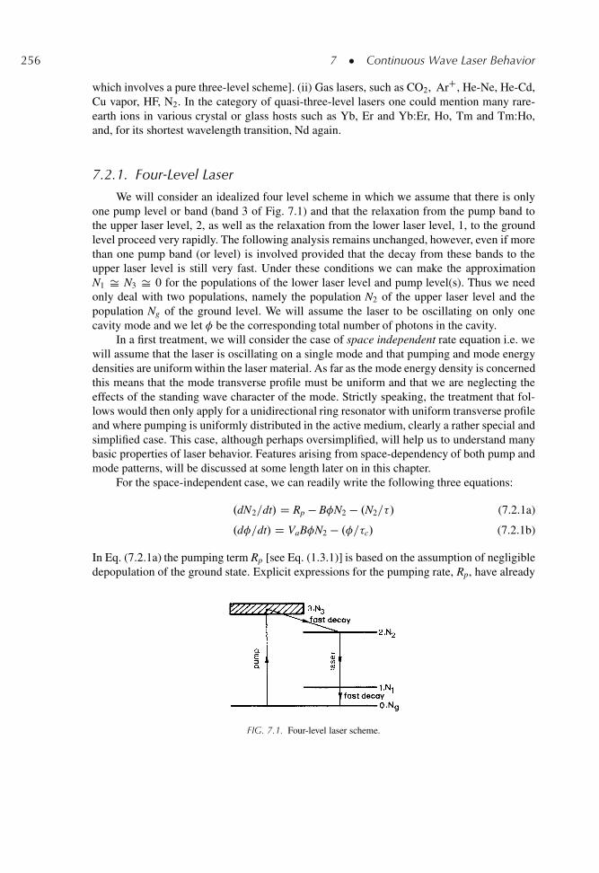
256 7 � Continuous Wave Laser Behavior
which involves a pure three-level scheme]. (ii) Gas lasers, such as CO2, ArC, He-Ne, He-Cd,Cu vapor, HF, N2. In the category of quasi-three-level lasers one could mention many rare-earth ions in various crystal or glass hosts such as Yb, Er and Yb:Er, Ho, Tm and Tm:Ho,and, for its shortest wavelength transition, Nd again.
7.2.1. Four-Level Laser
We will consider an idealized four level scheme in which we assume that there is onlyone pump level or band (band 3 of Fig. 7.1) and that the relaxation from the pump band tothe upper laser level, 2, as well as the relaxation from the lower laser level, 1, to the groundlevel proceed very rapidly. The following analysis remains unchanged, however, even if morethan one pump band (or level) is involved provided that the decay from these bands to theupper laser level is still very fast. Under these conditions we can make the approximationN1 Š N3 Š 0 for the populations of the lower laser level and pump level(s). Thus we needonly deal with two populations, namely the population N2 of the upper laser level and thepopulation Ng of the ground level. We will assume the laser to be oscillating on only onecavity mode and we let � be the corresponding total number of photons in the cavity.
In a first treatment, we will consider the case of space independent rate equation i.e. wewill assume that the laser is oscillating on a single mode and that pumping and mode energydensities are uniform within the laser material. As far as the mode energy density is concernedthis means that the mode transverse profile must be uniform and that we are neglecting theeffects of the standing wave character of the mode. Strictly speaking, the treatment that fol-lows would then only apply for a unidirectional ring resonator with uniform transverse profileand where pumping is uniformly distributed in the active medium, clearly a rather special andsimplified case. This case, although perhaps oversimplified, will help us to understand manybasic properties of laser behavior. Features arising from space-dependency of both pump andmode patterns, will be discussed at some length later on in this chapter.
For the space-independent case, we can readily write the following three equations:
.dN2=dt/ D Rp � B�N2 � .N2=�/ (7.2.1a)
.d�=dt/ D VaB�N2 � .�=�c/ (7.2.1b)
In Eq. (7.2.1a) the pumping term Rp [see Eq. (1.3.1)] is based on the assumption of negligibledepopulation of the ground state. Explicit expressions for the pumping rate, Rp, have already
FIG. 7.1. Four-level laser scheme.
7.2 � Rate Equations 257
been derived in the previous Chapter both for optical and electrical pumping. The term B�N2
in Eq. (7.2.1a) accounts for stimulated emission. It was shown in Chaps. 2 and 3 that thestimulated emission rate W is in fact proportional to the square of the magnitude of the electricfield of the e.m. wave, and hence W can also be taken to be proportional to �. The coefficientB will therefore be referred to as the stimulated transition rate per photon per mode. Thequantity � is the lifetime of the upper laser level, and, in general must take into account bothradiative and non-radiative processes [see Eq. (2.6.18)]. It must also be noted that the upperlaser level often consists of a combination of many strongly coupled sublevels. In this casethe lifetime � is intended to be the effective upper level lifetime, account being taken of thelifetimes of all upper state sublevels with a weight proportional to the corresponding sublevelpopulation [see Eq. (2.7.19c)]. In Eq. (7.2.1b) the term VaB�N2 represents the growth rate ofphoton population due to stimulated emission and is obtained by a simple balance argument.In Eq. (7.2.1a), in fact, the term B�N2 gives the rate of population decrease due to stimulatedemission. Since each stimulated-emission process creates a photon, B�N2 also representsthe number of photons created in the unit time and in the unit volume of the medium. Thephoton growth rate must then be VaB�N2, where Va is the volume of the mode in the activemedium. Finally, the term �=�c, where �c is the photon lifetime (see Sect. 5.3), accounts forthe disappearance of photons due to cavity losses.
Before proceeding it is worth pointing out that, in Eq. (7.2.1b), a term accounting forspontaneous emission has not been included. Since, as already mentioned in Chap. 1, laseraction is actually initiated by spontaneous emission, we would not expect Eq. (7.2.1) toaccount for the onset of laser oscillation. Indeed, if, at time t D 0, we put � D 0 on theright hand side of Eq. (7.2.1b), we get .d�=dt/ D 0 implying that laser action does not start.To try to account for spontaneous emission one might be tempted to apply simple considera-tions of balance, starting with the term N2=�r, �r being the radiative lifetime of level 2, whichis included in the term N2=� of (7.2.1a). It might then be thought that the appropriate termin Eq. (7.2.1b), to account for spontaneous emission, would be Va.N2=�r/. This is wrong,however. In fact, as seen in Chaps. 2 and 3, the spontaneously emitted light is distributed overthe entire frequency range corresponding to the gain bandwidth and, furthermore, emissionoccurs into a 4 solid angle. The spontaneous emission term which is needed in Eq. (7.2.1b)must, however, only include the fraction of the spontaneously emitted light that contributesto the given mode (i.e., that is emitted in the same angular direction and in the same spec-tral bandwidth of the mode). The correct expression for this term can only be obtained bya quantized treatment of radiation-matter interaction. The result is particularly simple andinstructive:.4/ in a quantum electrodynamics treatment, Eq. (7.2.1b) transforms to
.d�=dt/ D VaB.� C 1/N2 � .�=�c/ (7.2.2)
Thus everything behaves as if there were an extra photon in the term describing stimulatedemission. When the laser is oscillating, however, and unless very close to threshold, the num-ber of photons in the laser cavity may easily range between 1010 � 1016 for a cw laser, seeexample 7.1, and much more than this value for pulsed lasers. In the following analysis wewill therefore not consider this extra term arising from spontaneous emission, and insteadassume that an arbitrarily small number of photons �i, say �i D 1, is initially present in thecavity just to allow laser action to start.
258 7 � Continuous Wave Laser Behavior
We are now interested in deriving an explicit expression for the quantity B, the stimulatedemission coefficient per photon per mode, which is present in both Eqs. (7.2.1a) and (7.2.1b).So, we consider a resonator of length L in which an active medium of length l and refractiveindex n is inserted. Since, for the time being, we are considering a traveling wave beam, welet I be the intensity of this beam at a given cavity position and at time t D 0. Followingthe argument considered in Sect. 1.2, the intensity I0 after one cavity round trip is I0 D I �R1R2.1�Li/
2 exp.2�N2l/, where R1 and R2 are the power reflectivities of the two mirrors, Li isthe single pass internal loss of the cavity so that .1 �Li/
2 is the round trip cavity transmission,and exp.2�N2l/ is the round trip gain of the active medium. Note that, if the upper laser levelis either degenerate or consists of many strongly coupled sublevels, one should use here theeffective value of the cross section, as discussed in Sect. 2.7. We now write R1 D 1 � a1 � T1
and R2 D 1 � a2 � T2, where T1 and T2 are the power transmissions of the two mirrors anda1 and a2 are the corresponding fractional mirror losses. The change of intensity,I D I0 � I,for a cavity round trip will then be
I D Œ.1 � a1 � T1/.1 � a2 � T2/.1 � Li/2 exp.2� N2l/ � 1�I (7.2.3)
We will now assume that the mirror losses are equal .a1 D a2 D a/ and so small that we canput .1 � a � T1/ Š .1 � a/.1 � T1/ and .1 � a � T2/ Š .1 � a/.1 � T2/. Then (7.2.3) obviouslytransforms to
I D Œ.1 � T1/.1 � T2/.1 � a2/.1 � Li/2 exp.2� N2l/� 1�I (7.2.4)
Before proceeding it is convenient to introduce some new quantities, � (see Sect. 1.2),which can be described as the logarithmic loss per pass, namely, [compare with (1.2.4)]:
�1 D � ln.1 � T1/ (7.2.5)
�2 D � ln.1 � T2/ (7.2.6)
�i D �Œln.1 � a/C ln.1 � Li/� (7.2.7)
As already pointed out in Sect. 1.2, �1 and �2 are the logarithmic losses per pass due to themirror transmission and �i is the logarithmic internal loss per pass. For brevity, however, wewill simply call �1 and �2 the mirror losses and �i the internal loss. The logarithmic loss nota-tion proves to be the most convenient way of representing laser losses, given the exponentialcharacter of the laser gain. It should be noted, however, that, for small transmission values,one has � D � ln.1 � T/ Š T. Likewise, for very small values of a and Li one has fromEq. (7.2.7) �i Š a C Li, so that the quantities � really represent loss terms for the cavity.Obviously, one can see that the above approximations only hold for small values of cavityloss or mirror transmission. As an example, if we take T D 0.1 we get � D 0.104, i.e., � Š Twhile if we take T D 0.5 we get � D 0.695.
With the help of this logarithmic loss notation, we can also define a total (logarithmic)loss per pass � as
� D �i C Œ.�1 C �2/=2� (7.2.8)
7.2 � Rate Equations 259
and proceed by substituting Eqs. (7.2.5)–(7.2.8) into Eq. (7.2.4). Upon making the additionalassumption
Œ�N2l � �� � 1 (7.2.9)
then the exponential function resulting from Eq. (7.2.4) can be expanded as a power seriesto yield
I D 2Œ�N2l � ��I (7.2.10)
We now divide both sides of Eq. (7.2.10) by the timet taken for the light to make one cavityround trip, i.e., t D 2Le=c, where Le is the optical length of the resonator, given by
Le D L C .n � 1/l (7.2.11)
If the approximationI=t Š dI=dt is used, we get
dI
dtD�� lc
LeN2 � �c
Le
�I (7.2.12)
Since the number � of photons in the cavity is proportional to I, a comparison of Eq. (7.2.12)with Eq. (7.2.1b) gives
B D � lc
VaLeD �c
V(7.2.13)
�c D Le
� c(7.2.14)
where
V D .Le=l/Va (7.2.15)
will be referred to as the mode volume within the laser cavity (the mode diameter is takento be independent of the cavity longitudinal coordinate). Note that Eq. (7.2.14) generalizesthe expression for photon lifetime given in Sect. 5.3. Note also that, if the upper laser level isactually made of several strongly coupled sub-levels and if N2 is the total population of theupper laser level, then, according to the discussion in Sect. 2.7.2, the cross section � to be usedin Eq. (7.2.13) is the effective cross section, i.e., the true cross section times the fraction ofthe upper state population which is found in the sub-level from which laser action originates.
Once the explicit expressions for B and �c are obtained, then Eq. (7.2.1) provides, withinthe previous limitations and approximations, a description of both static and dynamic behaviorof a four level laser. To simplify notations, we will write N � N2 �N1 Š N2 as the populationinversion. From Eq. (7.2.1) we then get
dN
dtD Rp � B� N � N
�(7.2.16a)
d�
dtD�
BVaN � 1
�c
�� (7.2.16b)
260 7 � Continuous Wave Laser Behavior
These equations together with the expressions for B, �c and Va, given by Eqs. (7.2.13),(7.2.14) and (7.2.15) respectively, describe, for a four level-laser, the laser behavior bothin the c.w. and transient cases.
Before proceeding it is worth pointing out some caveats that apply to our considera-tions above. One such critical comment has already been made right at the beginning, namelythat the results strictly hold only for a laser oscillating with uniform pump and mode energydistributions in the active medium. This important point would seem to indicate a severe lim-itation to the usefulness of the above equations. However, the results obtained below, usingthis simple model, will be seen to be very useful for understanding some basic aspects of laserbehavior. Furthermore, at least for c.w. behavior, the much more complicated space-dependentcase leads, as we shall see, to rather similar results, whose relevance can then better under-stood by comparison with the space-independent model. A second critical remark relates tothe fact that these rate equations strictly apply only for single mode oscillation. For n oscillat-ing modes, in fact, one generally needs to write 2n differential equations for the amplitude andphase of the field modes to properly account for the beating terms among the various modes.In fact, under appropriate conditions of locking between the phases of the modes, this leadsto the phenomenon of mode-locking, to be described in next Chapter and which obviouslycannot be described within a rate equation treatment. However, when many modes with ran-dom phases are oscillating, the overall beam intensity can, to a first approximation, be takenas the sum of the intensities of all modes. For a uniform transverse pump profile, the superpo-sition of the mode transverse profiles will thus tend to produce a fairly uniform profile for theoverall beam. Furthermore, with the oscillation of many modes having different longitudinalpatterns, the corresponding total energy density will not show any pronounced standing wavepattern. In this case the picture can be greatly simplified by considering just one rate equationfor the total number of photons, �, i.e., summed over all modes, and Eqs. (7.2.16) can still beapplied in an approximate fashion. A third critical remark relates to the fact that, in writinge.g. Eq. (7.2.3), we have implicitly assumed that the population inversion, during laser action,is independent of the longitudinal z coordinate. Actually, for large values of laser gain, bothcounter-propagating beams show strong dependence on the z coordinate and similarly for theinversion. Under such conditions, the laser behavior should be treated on a pass-by-pass basisas first done by Rigrod (the so-called Rigrod analysis.5/). At least for the c.w. case whereEq. (7.2.9) can be taken to hold, however, the expression for the output power as obtainedby the Rigrod analysis coincides with that obtained via this far simpler treatment providedthat one makes use of the � notation, as indeed adopted here. For a pulsed laser, on the otherhand, Eq. (7.2.9) will hold only when the laser is not driven far above threshold. Otherwise,Eqs. (7.2.16) can no longer be applied and the dynamic behavior of the laser must be analyzedon a pass-by-pass basis, as in the Rigrod analysis..5/ A fourth and perhaps more serious remarkis that Eqs. (7.2.16) really do not apply to an inhomogeneously broadened line. To understandthis point, let us consider, for simplicity, a non-Doppler inhomogeneously-broadened transi-tion and assume the laser to be oscillating on a single frequency. The beam will then interactonly with that fraction of population whose resonance frequency coincides with the laser fre-quency and, at sufficiently high intensity, the saturated gain profile, likewise what shown inFig. 2.22 for an absorption profile, will show a hole located at this frequency. Clearly, in thiscase, the starting point of our analysis on beam amplification, namely Eq. (7.2.3) where N2
is the total upper state population, is no longer valid. The situation is even more complicated
7.2 � Rate Equations 261
for a Doppler-broadened inhomogeneous transition, where, if the laser is oscillating at a fre-quency sufficiently far from the central frequency of the transition, the right traveling beamand the left traveling beam interact with different sets of atoms or molecules. The c.w. behav-ior of an inhomogeneously broadened transition has been considered, notably by Casperson,.6/
and shown to give results considerably different from those obtained via Eqs. (7.2.16).
Example 7.1. Calculation of the number of cavity pho-tons in typical c.w. lasers We will first consider, as a lowpower example, a 50 cm long He-Ne laser, oscillating at� D 630 nm with an output power of 10 mW. The trans-mission of the output mirror, for this low gain laser, maytypically be T2 D 1% so that �2 D � ln.1 � T2/ Š 0.01.From Eq. (7.2.18) we then get � Š 1.06 � 1010 pho-tons. As a high power example, we consider a 10 kWCO2 laser oscillating at the wavelength of 10.6�m. Wetake a cavity length of Le D 150 cm and an output mirrortransmission, for this higher gain laser, of T2 D 45%. Weget �2 D � ln.1 � T2/ Š 0.598 and from Eq. (7.2.18)� Š 0.9 � 1016 photons.
Within the limitations discussed in theprevious paragraph, we now take Eqs. (7.2.16)as valid for a first order description of laserbehavior. Equations (7.2.16) then need to besolved under the appropriate conditions forthe case under examination. So, to describec.w. laser behavior, the case pertinent to thisChapter, we merely set the time derivativeon the left hand side of both equations equalto zero. To describe transient laser behavior,we need Rp D Rp.t/ to be specified and wealso need to know the initial conditions. Forinstance, if pumping is initiated at t D 0,the initial conditions will be N.0/ D 0 and�.0/ D �i where �i is a very small numberof initial photons simulating the effect of spontaneous emission (e.g., �i D 1). This will bediscussed in the next Chapter. For both c.w. and transient laser behavior, however, once � or�.t/ is known, the calculation of the output power through one of the cavity mirrors becomestraightforward. In fact, according to Eqs. (7.2.14) and (7.2.8) we can write
1
�cD �ic
LeC �1c
2LeC �2c
2Le(7.2.17)
If we now substitute Eq. (7.2.17) into the right hand side of Eq. (7.2.16b) we recognize thate.g., the term .�2c=2Le/� gives the rate of photon loss due to transmission through mirror 2.The output power through this mirror will therefore be given by
Pout D��2c
2Le
�.h�/� (7.2.18)
Thus the solution of Eqs. (7.2.16) allows not only to calculate the internal laser behaviorbut also, through the simple relation Eq. (7.2.18), one of the most important laser parameteri.e., the output power. Viceversa, if the output power is known, Eq. (7.2.18) can be used tocalculate the total number of cavity photons as shown in the following example.
7.2.2. Quasi-Three-Level Laser
In a quasi-three-level laser, the lower laser level, level 1 in Fig. 7.2, is a sub-level of theground level and all ground state sub-levels are assumed to be strongly coupled and hence inthermal equilibrium. Likewise, the upper laser level, level 2 in Fig. 7.2, is a sublevel of a set ofupper state sublevels which are also assumed to be in thermal equilibrium. In this case, we let
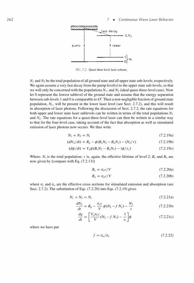
262 7 � Continuous Wave Laser Behavior
FIG. 7.2. Quasi-three-level laser scheme.
N1 and N2 be the total population of all ground state and all upper state sub-levels, respectively.We again assume a very fast decay from the pump level(s) to the upper state sub-levels, so thatwe will only be concerned with the populations N1, and N2 (ideal quasi-three-level case). Nowlet 0 represent the lowest sublevel of the ground state and assume that the energy separationbetween sub-levels 1 and 0 is comparable to kT. Then a non-negligible fraction of ground statepopulation, N1, will be present in the lower laser level (see Sect. 2.7.2), and this will resultin absorption of laser photons. Following the discussion of Sect. 2.7.2, the rate equations forboth upper and lower state laser sublevels can be written in terms of the total populations N1
and N2. The rate equations for a quasi-three-level laser can then be written in a similar wayto that for the four-level case, taking account of the fact that absorption as well as stimulatedemission of laser photons now occurs. We thus write
N1 C N2 D Nt (7.2.19a)
.dN2=dt/ D Rp � �.BeN2 � BaN1/ � .N2=�/ (7.2.19b)
.d�=dt/ D Va�.BeN2 � BaN1/ � .�=�c/ (7.2.19c)
Where: Nt is the total population; � is, again, the effective lifetime of level 2; Be and Ba arenow given by [compare with Eq. (7.2.13)]
Be D �ec=V (7.2.20a)
Ba D �ac=V (7.2.20b)
where �e and �a are the effective cross sections for stimulated emission and absorption (seeSect. 2.7.2). The substitution of Eqs. (7.2.20) into Eqs. (7.2.19) gives
N1 C N2 D Nt (7.2.21a)
dN2
dtD Rp � �ec
V�.N2 � f N1/� N2
�(7.2.21b)
dq
dtD�
Va�ec
V.N2 � f N1/ � 1
�c
�� (7.2.21c)
where we have put
f D �a=�e (7.2.22)
7.3 � Threshold Conditions and Output Power: Four-Level Laser 263
Equations (7.2.21b) and (7.2.21c) suggest that we may now define a population inversion N as
N D N2 � fN1 (7.2.23)
Using the pair of Eqs. (7.2.21a) and (7.2.23) one can obtain N1 and N2 in terms of N and Nt.The three Eqs. (7.2.21) can then be reduced to just two equations in the variables � and N.After some straightforward manipulation one obtains
dN
dtD Rp.1 C f / � .�e C �a/c
V� N � f Nt C N
�(7.2.24a)
d�
dtD�
Va�ec
VN � 1
�c
�� (7.2.24b)
Within the limits discussed for the validity of Eqs. (7.2.16) and (7.2.24) describe the staticand dynamic behavior of a quasi-three-level laser�. In the case of transient laser behavior andif pumping is initiated at t D 0, Eqs. (7.2.24) must be solved with the initial conditions N.0/ D�fN1 and �.0/ D �i Š 1. Note that the photon rate equations for four-level, Eq. (7.2.16b),and quasi-three-level, Eq. (7.2.24b), lasers are the same. The rate equation for the populationinversion is somewhat different, however. In particular, the stimulated term for a quasi-three-level laser is a factor .�e C �a/=�e larger than that of a four-level laser. To understand thisresult, consider a unit volume, Va D 1, and assume that, in a given time t, one photonhas been created, by the stimulated processes, in this volume. According to Eq. (7.2.24b),this implies that .�ec0N�=V/t D 1. Using this result in Eq. (7.2.24a) one then sees that,correspondingly, the inversion N decreases by an amount equal to N D .�e C �a/=�e. Onethus hasN > 1, and this is understood when one notices that, due to this stimulated process,N2 has decreased by 1 while N1 has been increased by 1, so that, according to Eq. (7.2.23), thedecrease of N must indeed be larger than 1. By contrast, for a four-level laser, the emission ofa photon implies that N2 decreases by 1 while N1 remains essentially unchanged (i.e., zero)on account of the fast 1 ! 0 decay. Thus, in this case, the decrease of N is simply equal to 1.Note also that, as expected, Eqs. (7.2.24) reduce to (7.2.16) when �a and hence f are set equalto zero.
Within the limits of a space-independent rate equation treatment, Eqs. (7.2.24) thusrepresent the final result of our calculation for a quasi-three-level level laser. For both c.w.and transient case, once N and � are obtained by solving these equations with the appro-priate boundary conditions, the output power through e.g. mirror 2 is again obtained fromEq. (7.2.18).
7.3. THRESHOLD CONDITIONS AND OUTPUT POWER:FOUR-LEVEL LASER
In this section we will investigate, for a four-level laser, the threshold conditions and theoutput power for a c.w. laser i.e. when Rp is time-independent. We first consider the behav-ior corresponding to the space-independent rate equations described previously. The results
� One should note that, as a quasi-3-level laser becomes progressively closer to a pure 3-level laser, the assumptionthat the ground state population is changed negligibly by the pumping process will eventually not be justified andthe pump rate Rp could not be taken to be constant any more.
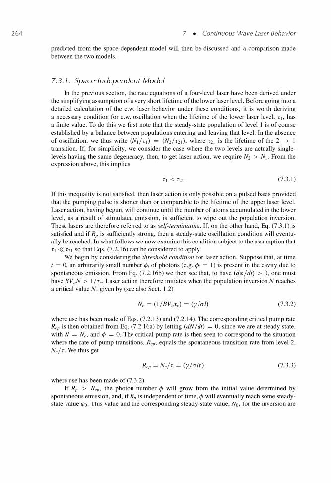
264 7 � Continuous Wave Laser Behavior
predicted from the space-dependent model will then be discussed and a comparison madebetween the two models.
7.3.1. Space-Independent Model
In the previous section, the rate equations of a four-level laser have been derived underthe simplifying assumption of a very short lifetime of the lower laser level. Before going into adetailed calculation of the c.w. laser behavior under these conditions, it is worth derivinga necessary condition for c.w. oscillation when the lifetime of the lower laser level, �1, hasa finite value. To do this we first note that the steady-state population of level 1 is of courseestablished by a balance between populations entering and leaving that level. In the absenceof oscillation, we thus write .N1=�1/ D .N2=�21/, where �21 is the lifetime of the 2 ! 1transition. If, for simplicity, we consider the case where the two levels are actually single-levels having the same degeneracy, then, to get laser action, we require N2 > N1. From theexpression above, this implies
�1 < �21 (7.3.1)
If this inequality is not satisfied, then laser action is only possible on a pulsed basis providedthat the pumping pulse is shorter than or comparable to the lifetime of the upper laser level.Laser action, having begun, will continue until the number of atoms accumulated in the lowerlevel, as a result of stimulated emission, is sufficient to wipe out the population inversion.These lasers are therefore referred to as self-terminating. If, on the other hand, Eq. (7.3.1) issatisfied and if Rp is sufficiently strong, then a steady-state oscillation condition will eventu-ally be reached. In what follows we now examine this condition subject to the assumption that�1 � �21 so that Eqs. (7.2.16) can be considered to apply.
We begin by considering the threshold condition for laser action. Suppose that, at timet D 0, an arbitrarily small number �i of photons (e.g. �i D 1) is present in the cavity due tospontaneous emission. From Eq. (7.2.16b) we then see that, to have .d�=dt/ > 0, one musthave BVaN > 1=�c. Laser action therefore initiates when the population inversion N reachesa critical value Nc given by (see also Sect. 1.2)
Nc D .1=BVa�c/ D .�=� l/ (7.3.2)
where use has been made of Eqs. (7.2.13) and (7.2.14). The corresponding critical pump rateRcp is then obtained from Eq. (7.2.16a) by letting .dN=dt/ D 0, since we are at steady state,with N D Nc, and � D 0. The critical pump rate is then seen to correspond to the situationwhere the rate of pump transitions, Rcp, equals the spontaneous transition rate from level 2,Nc=� . We thus get
Rcp D Nc=� D .�=� l�/ (7.3.3)
where use has been made of (7.3.2).If Rp > Rcp, the photon number � will grow from the initial value determined by
spontaneous emission, and, if Rp is independent of time, � will eventually reach some steady-state value �0. This value and the corresponding steady-state value, N0, for the inversion are
7.3 � Threshold Conditions and Output Power: Four-Level Laser 265
FIG. 7.3. Qualitative behavior of the population inversion N and total number of cavity photons � as a function ofthe pump rate Rp.
obtained from Eqs. (7.2.16) by setting .dN=dt/ D .d�=dt/ D 0. This gives
N0 D .1=BVa�c/ D .�=� l/ (7.3.4a)
�0 D Va�cŒRp � .N0=�/� (7.3.4b)
Note that, to obtain Eq. (7.3.4b), use has been made of Eqs. (7.3.4a), (7.2.15) and (7.2.14).Equations (7.3.4) describe the c.w. behavior of a four level laser. We will now examine
these equations in some detail. Comparing Eq. (7.3.4a) with Eq. (7.3.2) one can first observethat, even when Rp > Rcp, one has N0 D Nc, i.e., the steady-state inversion always equals thecritical or threshold inversion. To get a better understanding of this result, we show in Fig. 7.3a plot of both N and � vs the pump rate Rp. When Rp < Rcp, then �0 D 0 and the inversion,N, increases linearly with Rp. When Rp D Rcp, one obviously has N D Nc and �0 D 0 stillapplies. If now Rp is increased above Rcp, Eqs. (7.3.4) show that, while N0 remains fixed atthe critical inversion, �0 increases linearly with Rp. In other words, the pump rate increasesthe inversion (i.e. the energy stored in the material), below threshold, while it increases thenumber of photons (i.e., the e.m energy stored in the cavity), above threshold.
We can now recast Eq. (7.3.4b) in a somewhat simpler form if we take the term .N0=�/ D.Nc=�/ D Rcp outside the square brackets. We obtain
�0 D .VaN0/�c
�.x � 1/ (7.3.5)
where
x D Rp=Rcp (7.3.6)
is the amount by which the pump rate exceeds the threshold pump rate. One can now see that,both for optical and electrical pumping, one can write
x D Pp=Pth (7.3.7)
where Pp is the pumping power and Pth is its threshold value. Using Eqs. (7.3.7) and (7.3.4a)in Eq. (7.3.5), this equation can be transformed to a somewhat more useful form:
�0 D Ab�
�
�c
�
�Pp
Pth� 1
�(7.3.8)
266 7 � Continuous Wave Laser Behavior
where Ab D .Va=l/ is the cross-sectional area of the mode (the beam area) which is assumedto be smaller than or equal to the cross-sectional area, A D .V=l/, of the active medium.
We now go on to derive an expression for the output power. From Eqs. (7.2.18)and (7.3.8) we obtain
Pout D .AbIs/��2
2
� � Pp
Pth� 1
�(7.3.9)
where Is D h�=�� is the saturation intensity for a four-level system [see Eq. (2.8.24)]. Ifmirror 1 is totally reflecting, this expression agrees with that of Rigrod,.5/ obtained using apass-by-pass analysis. Since a plot of Pout versus Pp yields a straight line intercepting the Pp
axis at Pp D Pth, one can define the laser slope efficiency as
�s D dPout=dPp (7.3.10)
and �s turns out to be constant for a given laser configuration. With the help of the previousexpressions and of the equations derived in Chap. 6, we can get a very useful and instructiveexpression for �s. Thus, inserting Pout from Eq. (7.3.9) into Eq. (7.3.10), we begin by writing
�s D Ab h�
��
�2
2
1
Pth(7.3.11)
For both lamp pumping and electrical pumping, using Eq. (6.2.6) or (6.4.26) in Eq. (7.3.3),we obtain
Pth D �
�p
�h�mp
�
� �A
�
�(7.3.12)
where we recall that �mp is the frequency difference between the upper laser level and theground level and A is the area of the active medium. From Eqs. (7.3.11) and (7.3.12) oneobtains
�s D �p
��2
2�
� �h�
h�mp
� �Ab
A
�(7.3.13)
One can then write
�s D �p �c �q �t (7.3.14)
where: (1) �p is the pump efficiency. (2) �c D �2=2� represents the fraction of gener-ated photons coupled out of the cavity, which one can call the output coupling efficiency.Note that �c is always smaller than 1 and it reaches the value 1 when �1 D �i D 0. (3)�q D h�=h�mp gives the fraction of the minimum pump energy which is transformed intolaser energy, referred to as the laser quantum efficiency. (4) �t D Ab=A, gives the frac-tion of the active medium cross-section which is utilized by the beam cross section andmay be called the transverse utilization factor of the active medium or the transverse effi-ciency. Note that the whole of the active medium is assumed to be pumped uniformly, inour case.
7.3 � Threshold Conditions and Output Power: Four-Level Laser 267
Example 7.2. CW laser behavior of a lamp pumped high-power Nd:YAG laser We consider the lasersystem of Fig. 7.4, where a 6.35 mm diameter, 7.5 cm long Nd:YAG rod, with 1% atomic concentrationof the active Nd ions, is pumped in an elliptical pump chamber by a high-pressure Kr lamp. The lasercavity consists of two plane mirrors spaced by 50 cm. The reflectivity of one mirror is R1 D 100% whilethat of the output coupling mirror is R2 D 85%. A typical curve of the output power, Pout, through mirror2 (in multimode operation) vs electrical pump power, Pp, to the Kr lamp is shown in Fig. 7.5..7/ Notethat one is dealing with a reasonably high power c.w. Nd:YAG laser with an output power exceeding200 W. One may also observe that, since the laser is oscillating on many transverse and longitudinalmodes then, according to the discussion in Sect. 7.2.1, it is reasonable to compare the experimental resultswith the theoretical predictions given by the preceding space-independent rate equation treatment. In fact,except for input powers just above threshold, the experimental points of Fig. 7.5 indeed show a linearrelationship between output and input powers as predicted by Eq. (7.3.9). From the linear part of thecurve, an extrapolated threshold of Pth D 2.2 kW is obtained. Above threshold, the output vs input powerrelation can be fitted by the equation
Pout D 53Œ.Pp=Pth/ � 1� (7.3.15)
where Pout is expressed in watts. The slope efficiency is then easily obtained from Eq. (7.3.15) as�s D .dPout=dPp/D 53=Pth D 2.4%. Equation (7.3.15) can be readily compared to Eq. (7.3.9) once weremember that, as discussed in example 2.10, the effective values of cross section and upper level life-time for the �D 1.06�m transition in Nd:YAG can be taken to be � D 2.8 � 10�19 cm2 and � D 230�s,respectively. The energy of the photon, at this wavelength, is obtained as h�D 3.973 � 10�19 �.0.5=1.06/D1.87 � 10�19 J, where 3.973 � 10�19 J is the energy of a photon with a wavelength of 0.5�m(see Appendix H). We then obtain the value of the saturation intensity as Is D h�=�� D 2.9 kW=cm2. Wenow take R2 D .1 � a2 � T2/ Š .1 � T2/ since, for a good multilayer coating, mirror absorption, a2, maybe less than 0.1%. We then get �2 D � ln R2 D 0.162. Comparison of Eq. (7.3.15) with Eq. (7.3.9) thengives Ab Š 0.23 cm2, to be compared with the cross-sectional area of the rod A Š 0.317 cm2.
To compare the measured slope efficiency and the extrapolated threshold with the values predictedby calculation, we need to know � , i.e., �i. Now, since �1 D 0, (7.3.12) with the help of (7.2.8) can berearranged as
� ln R2
2C �i D �p
��A
� � Pth�
h�mp
�(7.3.16)
Thus, if several measurements are made of the threshold pump power at different mirror reflectivities R2,a plot of �2 D � lnR2 vs Pth should yield a straight line. In fact, this is what is found experimentally, asshown in Fig. 7.6. The intercept of this straight line with the �2 axis gives, according to Eq. (7.3.16), thevalue of the internal losses (Findlay and Clay analysis.9/). From Fig. 7.6 we get �i Š 0.038, which givesa total loss � D .�2=2/C �i Š 0.12.
Once the total losses are known, we can use Eq. (7.3.14) to compare the measured slope effi-ciency, �s D 2.4%, with the theoretical predictions. We take, in fact, �c D �2=2� Š 0.68. We also take�q D�mp=�D 0.89, where �mp D 0.94�m is the wavelength corresponding to the transition from theupper laser level to the ground level (see Fig. 2.15) in Nd:YAG, and, according to the previous calculation,�t D Ab=A. Š 0.72. From Eq. (7.3.14) we get �p D 5.5%, which appears to be a reasonable value of pumpefficiency for Kr pumping (see also Table 6.1). The predicted value of Pth can now be readily obtainedfrom Eq. (7.3.12) once we take into account that h�mp Š 2.11 � 10�19 J. We obtain Pth Š 2.26 kW, in
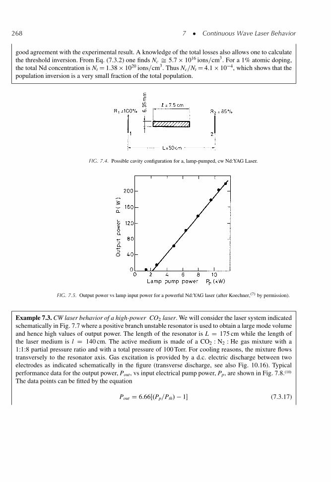
268 7 � Continuous Wave Laser Behavior
good agreement with the experimental result. A knowledge of the total losses also allows one to calculatethe threshold inversion. From Eq. (7.3.2) one finds Nc Š 5.7 � 1016 ions=cm3. For a 1% atomic doping,the total Nd concentration is Nt D 1.38 � 1020 ions=cm3. Thus Nc=Nt D 4.1 � 10�4, which shows that thepopulation inversion is a very small fraction of the total population.
FIG. 7.4. Possible cavity configuration for a, lamp-pumped, cw Nd:YAG Laser.
FIG. 7.5. Output power vs lamp input power for a powerful Nd:YAG laser (after Koechner,.7/ by permission).
Example 7.3. CW laser behavior of a high-power CO2 laser. We will consider the laser system indicatedschematically in Fig. 7.7 where a positive branch unstable resonator is used to obtain a large mode volumeand hence high values of output power. The length of the resonator is L D 175 cm while the length ofthe laser medium is l D 140 cm. The active medium is made of a CO2 : N2 : He gas mixture with a1:1:8 partial pressure ratio and with a total pressure of 100 Torr. For cooling reasons, the mixture flowstransversely to the resonator axis. Gas excitation is provided by a d.c. electric discharge between twoelectrodes as indicated schematically in the figure (transverse discharge, see also Fig. 10.16). Typicalperformance data for the output power, Pout, vs input electrical pump power, Pp, are shown in Fig. 7.8..10/
The data points can be fitted by the equation
Pout D 6.66Œ.Pp=Pth/ � 1� (7.3.17)
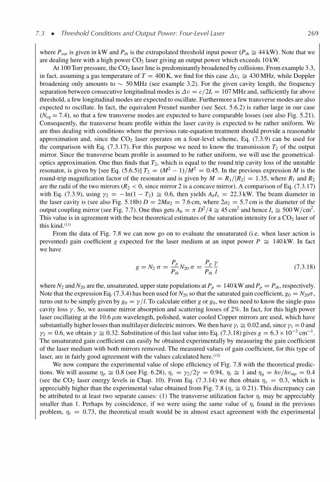
7.3 � Threshold Conditions and Output Power: Four-Level Laser 269
where Pout is given in kW and Pth is the extrapolated threshold input power .Pth Š 44 kW/. Note that weare dealing here with a high power CO2 laser giving an output power which exceeds 10 kW.
At 100 Torr pressure, the CO2 laser line is predominantly broadened by collisions. From example 3.3,in fact, assuming a gas temperature of T D 400 K, we find for this case �c Š 430 MHz, while Dopplerbroadening only amounts to � 50 MHz (see example 3.2). For the given cavity length, the frequencyseparation between consecutive longitudinal modes is� D c=2L D 107 MHz and, sufficiently far abovethreshold, a few longitudinal modes are expected to oscillate. Furthermore a few transverse modes are alsoexpected to oscillate. In fact, the equivalent Fresnel number (see Sect. 5.6.2) is rather large in our case.Neq D 7.4/, so that a few transverse modes are expected to have comparable losses (see also Fig. 5.21).Consequently, the transverse beam profile within the laser cavity is expected to be rather uniform. Weare thus dealing with conditions where the previous rate-equation treatment should provide a reasonableapproximation and, since the CO2 laser operates on a four-level scheme, Eq. (7.3.9) can be used forthe comparison with Eq. (7.3.17). For this purpose we need to know the transmission T2 of the outputmirror. Since the transverse beam profile is assumed to be rather uniform, we will use the geometrical-optics approximation. One thus finds that T2, which is equal to the round trip cavity loss of the unstableresonator, is given by [see Eq. (5.6.5)] T2 D .M2 � 1/=M2 D 0.45. In the previous expression M is theround-trip magnification factor of the resonator and is given by M D R1=jR2j D 1.35, where R1 and R2
are the radii of the two mirrors (R2 < 0, since mirror 2 is a concave mirror). A comparison of Eq. (7.3.17)with Eq. (7.3.9), using �2 D � ln.1 � T2/ Š 0.6, then yields AbIs D 22.3 kW. The beam diameter inthe laser cavity is (see also Fig. 5.18b) D D 2Ma2 D 7.6 cm, where 2a2 D 5.7 cm is the diameter of theoutput coupling mirror (see Fig. 7.7). One thus gets Ab D D2=4 Š 45 cm2 and hence Is Š 500 W=cm2.This value is in agreement with the best theoretical estimates of the saturation intensity for a CO2 laser ofthis kind..11/
From the data of Fig. 7.8 we can now go on to evaluate the unsaturated (i.e. when laser action isprevented) gain coefficient g expected for the laser medium at an input power P Š 140 kW. In factwe have
g D N2 � D Pp
PthN20 � D Pp
Pth
�
l(7.3.18)
where N2 and N20 are the, unsaturated, upper state populations at Pp D 140 kW and Pp D Pth, respectively.Note that the expression Eq. (7.3.4) has been used for N20 so that the saturated gain coefficient, g0 D N20� ,turns out to be simply given by g0 D �=l. To calculate either g or g0, we thus need to know the single-passcavity loss � . So, we assume mirror absorption and scattering losses of 2%. In fact, for this high powerlaser oscillating at the 10.6�m wavelength, polished, water cooled Copper mirrors are used, which havesubstantially higher losses than multilayer dielectric mirrors. We then have �i Š 0.02 and, since �1 D 0 and�2 D 0.6, we obtain � Š 0.32. Substitution of this last value into Eq. (7.3.18) gives g D 6.3 � 10�3 cm�1.The unsaturated gain coefficient can easily be obtained experimentally by measuring the gain coefficientof the laser medium with both mirrors removed. The measured values of gain coefficient, for this type oflaser, are in fairly good agreement with the values calculated here..12/
We now compare the experimental value of slope efficiency of Fig. 7.8 with the theoretical predic-tions. We will assume �p Š 0.8 (see Fig. 6.28), �c D �2=2� D 0.94, �t Š 1 and �q D h�=h�mp D 0.4(see the CO2 laser energy levels in Chap. 10). From Eq. (7.3.14) we then obtain �s D 0.3, which isappreciably higher than the experimental value obtained from Fig. 7.8 .�s Š 0.21/. This discrepancy canbe attributed to at least two separate causes: (1) The transverse utilization factor �t may be appreciablysmaller than 1. Perhaps by coincidence, if we were using the same value of �t found in the previousproblem, �t D 0.73, the theoretical result would be in almost exact agreement with the experimental
270 7 � Continuous Wave Laser Behavior
one. (2) The data of Fig. 7.7 refer to a partially closed-cycle system and, in this case, the products ofthe electric discharge (mostly CO and O2) are likely to accumulate in the gas mixture, thus reducing thepumping efficiency below the theoretical value of 80%. Actually, it is a matter of fact that slope efficien-cies larger than � 20% are seldom found in practice for any CO2 laser. The discussion presented abovethus helps ones understanding of how the slope efficiency is further reduced from the already reducedvalue established by the quantum efficiency .�q D 40%/.
FIG. 7.6. Threshold pump power as a function of mirror reflectivity (after Koechner,.8/ by permission).
FIG. 7.7. Possible cavity configuration for a powerful cw CO2 laser.
7.3.2. Space-Dependent Model
We shall consider now the case where the mode distribution and the pump rate arespatially dependent. In this case the inversion will also be spatially dependent and the rateequation treatment becomes more complicated. We will therefore limit ourselves, here, toa discussion of the most relevant results and refer to Appendix E for a detailed treatment.We assume a cylindrical symmetry and let u be the field amplitude of the given mode,
7.3 � Threshold Conditions and Output Power: Four-Level Laser 271
FIG. 7.8. Output power, P, versus electrical discharge power, Pp, for a powerful cw CO2 laser.
normalized to its peak value. For simplicity, we will take u to be independent of the lon-gitudinal coordinate, z, along the resonator while we will generally take the pump rate to bedependent on both radial and longitudinal coordinates, i.e. Rp D Rp.r, z/.
As far as the threshold conditions are concerned, it will be shown in the Appendix E thatEq. (7.3.2) still holds for the average value of N i.e.,
<N>c D .�=� l/ (7.3.19)
where the average is taken over the squared amplitude of the field distribution, viz [see alsoEq. (6.3.17)]
<N> D0@Z
a
Njuj2dV
1A =
Za
juj2dV (7.3.20)
and the integrals are taken over the volume of the active medium. At each point of the activemedium, below or at threshold, an equilibrium must exist between the number of atomsraised by the pumping process and those decaying spontaneously i.e. Rp.r, z/ D N.r, z/=� .At threshold, we then have
<Rp>c D <N>c
�D �
� l�(7.3.21)
where<Rp> is the average of Rp.r, z/ over the squared amplitude of the field distribution [seeEq. (6.3.8)] and where Eq. (7.3.19) has been used.
Above threshold, from the condition d�=dt D 0, one now finds that the average gainmust equal total losses i.e.
� l<N>0 D � D � l<N>c (7.3.22)
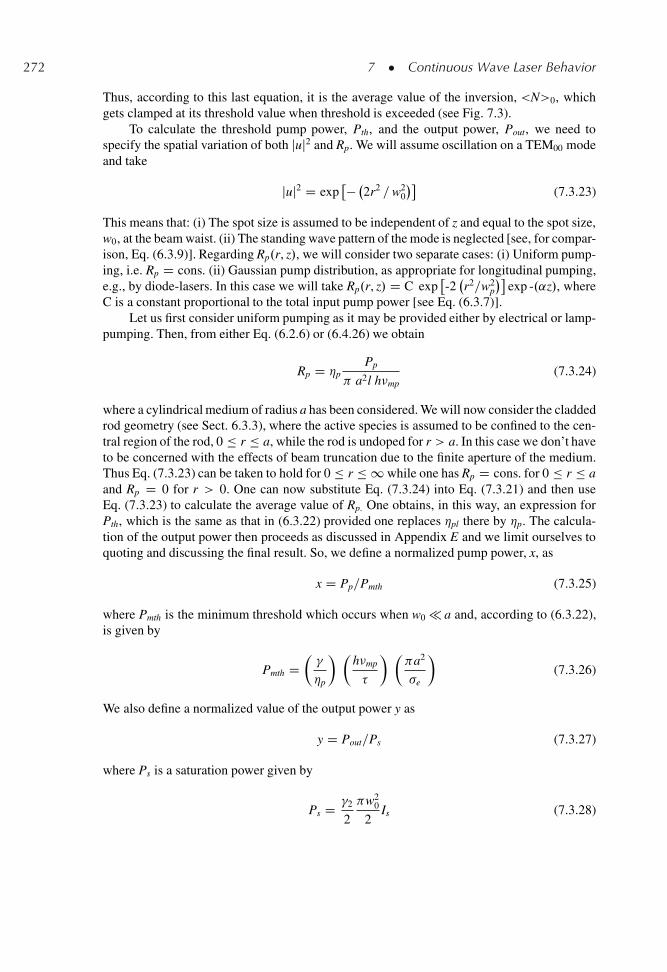
272 7 � Continuous Wave Laser Behavior
Thus, according to this last equation, it is the average value of the inversion, <N>0, whichgets clamped at its threshold value when threshold is exceeded (see Fig. 7.3).
To calculate the threshold pump power, Pth, and the output power, Pout, we need tospecify the spatial variation of both juj2 and Rp. We will assume oscillation on a TEM00 modeand take
juj2 D exp�� 2r2 =w2
0
�(7.3.23)
This means that: (i) The spot size is assumed to be independent of z and equal to the spot size,w0, at the beam waist. (ii) The standing wave pattern of the mode is neglected [see, for compar-ison, Eq. (6.3.9)]. Regarding Rp.r, z/, we will consider two separate cases: (i) Uniform pump-ing, i.e. Rp D cons. (ii) Gaussian pump distribution, as appropriate for longitudinal pumping,e.g., by diode-lasers. In this case we will take Rp.r, z/ D C exp
�-2r2=w2
p
�exp -.˛z/, where
C is a constant proportional to the total input pump power [see Eq. (6.3.7)].Let us first consider uniform pumping as it may be provided either by electrical or lamp-
pumping. Then, from either Eq. (6.2.6) or (6.4.26) we obtain
Rp D �pPp
a2l h�mp(7.3.24)
where a cylindrical medium of radius a has been considered. We will now consider the claddedrod geometry (see Sect. 6.3.3), where the active species is assumed to be confined to the cen-tral region of the rod, 0 r a, while the rod is undoped for r > a. In this case we don’t haveto be concerned with the effects of beam truncation due to the finite aperture of the medium.Thus Eq. (7.3.23) can be taken to hold for 0 r 1 while one has Rp D cons. for 0 r aand Rp D 0 for r > 0. One can now substitute Eq. (7.3.24) into Eq. (7.3.21) and then useEq. (7.3.23) to calculate the average value of Rp. One obtains, in this way, an expression forPth, which is the same as that in (6.3.22) provided one replaces �pl there by �p. The calcula-tion of the output power then proceeds as discussed in Appendix E and we limit ourselves toquoting and discussing the final result. So, we define a normalized pump power, x, as
x D Pp=Pmth (7.3.25)
where Pmth is the minimum threshold which occurs when w0 � a and, according to (6.3.22),is given by
Pmth D��
�p
� �h�mp
�
� � a2
�e
�(7.3.26)
We also define a normalized value of the output power y as
y D Pout=Ps (7.3.27)
where Ps is a saturation power given by
Ps D �2
2
w20
2Is (7.3.28)
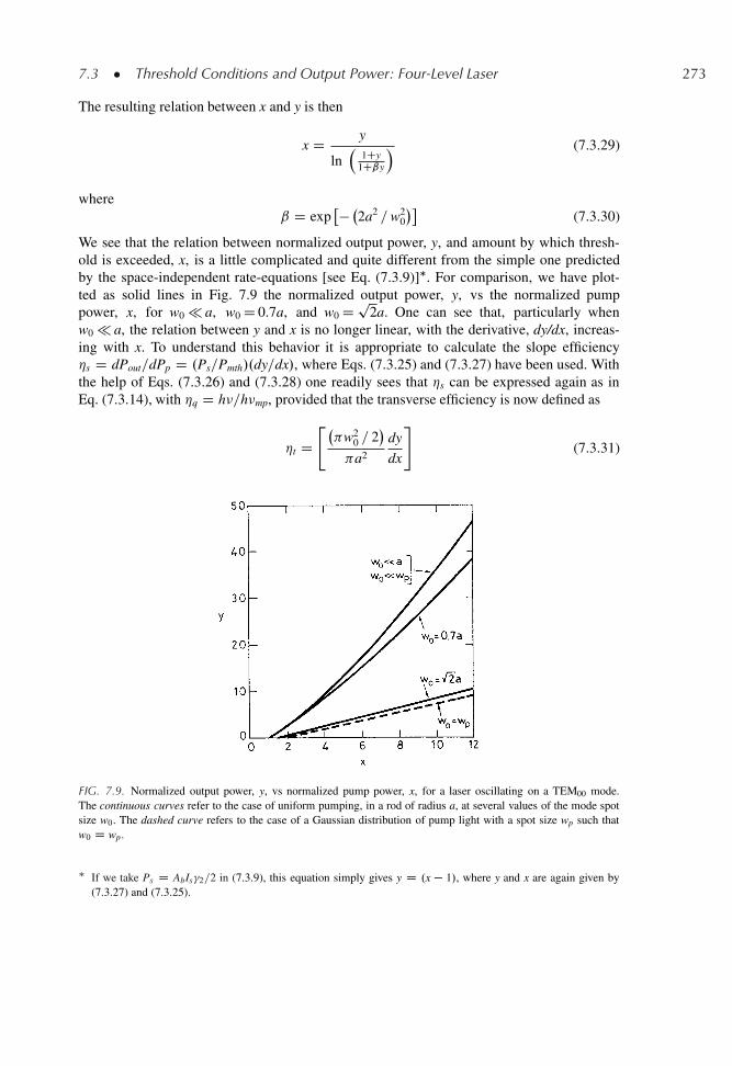
7.3 � Threshold Conditions and Output Power: Four-Level Laser 273
The resulting relation between x and y is then
x D y
ln�
1Cy1Cˇy
� (7.3.29)
whereˇ D exp
�� 2a2 =w20
�(7.3.30)
We see that the relation between normalized output power, y, and amount by which thresh-old is exceeded, x, is a little complicated and quite different from the simple one predictedby the space-independent rate-equations [see Eq. (7.3.9)]�. For comparison, we have plot-ted as solid lines in Fig. 7.9 the normalized output power, y, vs the normalized pumppower, x, for w0 � a, w0 D 0.7a, and w0 D p
2a. One can see that, particularly whenw0 � a, the relation between y and x is no longer linear, with the derivative, dy/dx, increas-ing with x. To understand this behavior it is appropriate to calculate the slope efficiency�s D dPout=dPp D .Ps=Pmth/.dy=dx/, where Eqs. (7.3.25) and (7.3.27) have been used. Withthe help of Eqs. (7.3.26) and (7.3.28) one readily sees that �s can be expressed again as inEq. (7.3.14), with �q D h�=h�mp, provided that the transverse efficiency is now defined as
�t D" w2
0 = 2�
a2
dy
dx
#(7.3.31)
FIG. 7.9. Normalized output power, y, vs normalized pump power, x, for a laser oscillating on a TEM00 mode.The continuous curves refer to the case of uniform pumping, in a rod of radius a, at several values of the mode spotsize w0. The dashed curve refers to the case of a Gaussian distribution of pump light with a spot size wp such thatw0 D wp.
� If we take Ps D AbIs�2=2 in (7.3.9), this equation simply gives y D .x � 1/, where y and x are again given by(7.3.27) and (7.3.25).
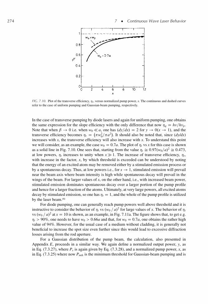
274 7 � Continuous Wave Laser Behavior
FIG. 7.10. Plot of the transverse efficiency, �t , versus normalized pump power, x. The continuous and dashed curvesrefer to the case of uniform pumping and Gaussian-beam pumping, respectively.
In the case of transverse pumping by diode lasers and again for uniform pumping, one obtainsthe same expression for the slope efficiency with the only difference that now �q D h�=h�p.Note that when ˇ ! 0 i.e. when w0 � a, one has .dy=dx/ D 2 for y ! 0.x ! 1/, and thetransverse efficiency becomes �t D
w20= a2
�. It should also be noted that, since (dy/dx)
increases with x, the transverse efficiency will also increase with x. To understand this pointwe will consider, as an example, the case w0 D 0.7a. The plot of �t vs x for this case is shownas a solid line in Fig. 7.10. One sees that, starting from the value �t Š 0.97.w0=a/2 Š 0.473,at low powers, �t increases to unity when x � 1. The increase of transverse efficiency, �t,with increase in the factor, x, by which threshold is exceeded can be understood by notingthat the energy of an excited atom may be removed either by a stimulated emission process orby a spontaneous decay. Thus, at low powers i.e., for x ! 1, stimulated emission will prevailnear the beam axis where beam intensity is high while spontaneous decay will prevail in thewings of the beam. For larger values of x, on the other hand, i.e., with increased beam power,stimulated emission dominates spontaneous decay over a larger portion of the pump profileand hence for a larger fraction of the atoms. Ultimately, at very large powers, all excited atomsdecay by stimulated emission, so one has �t D 1, and the whole of the pump profile is utilizedby the laser beam..6/
For diode pumping, one can generally reach pump powers well above threshold and it isinstructive to consider the behavior of �t vs .w0 = a/2 for large values of x. The behavior of �t
vs .w0 = a/2 at x D 10 is shown, as an example, in Fig. 7.11a. The figure shows that, to get e.g.�t > 90%, one needs to have w0 > 0.66a and that, for w0 D 0.7a, one obtains the rather highvalue of 94%. However, for the usual case of a medium without cladding, it is generally notbeneficial to increase the spot size even further since this would lead to excessive diffractionlosses arising from the rod aperture.
For a Gaussian distribution of the pump beam, the calculation, also presented inAppendix E, proceeds in a similar way. We again define a normalized output power, y, asin Eq. (7.3.27), where Ps is again given by Eq. (7.3.28), and a normalized pump power, x, asin Eq. (7.3.25) where now Pmth is the minimum threshold for Gaussian-beam pumping and is
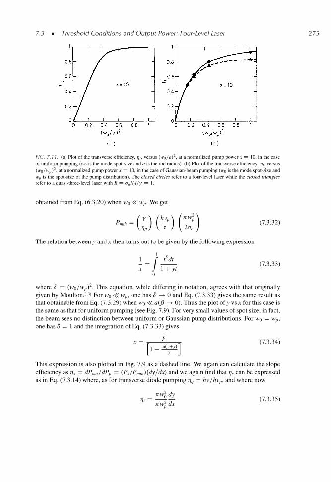
7.3 � Threshold Conditions and Output Power: Four-Level Laser 275
FIG. 7.11. (a) Plot of the transverse efficiency, �t, versus .w0=a/2, at a normalized pump power x D 10, in the caseof uniform pumping (w0 is the mode spot-size and a is the rod radius). (b) Plot of the transverse efficiency, �t, versus.w0=wp/
2, at a normalized pump power x D 10, in the case of Gaussian-beam pumping (w0 is the mode spot-size andwp is the spot-size of the pump distribution). The closed circles refer to a four-level laser while the closed trianglesrefer to a quasi-three-level laser with B D �aNtl=� D 1.
obtained from Eq. (6.3.20) when w0 � wp. We get
Pmth D��
�p
� �h�p
�
� w2
p
2�e
!(7.3.32)
The relation between y and x then turns out to be given by the following expression
1
xD
1Z0
tı dt
1 C yt(7.3.33)
where ı D .w0=wp/2. This equation, while differing in notation, agrees with that originally
given by Moulton..13/ For w0 � wp, one has ı ! 0 and Eq. (7.3.33) gives the same result asthat obtainable from Eq. (7.3.29) when w0 � a.ˇ ! 0/. Thus the plot of y vs x for this case isthe same as that for uniform pumping (see Fig. 7.9). For very small values of spot size, in fact,the beam sees no distinction between uniform or Gaussian pump distributions. For w0 D wp,one has ı D 1 and the integration of Eq. (7.3.33) gives
x D yh1 � ln.1Cy/
y
i (7.3.34)
This expression is also plotted in Fig. 7.9 as a dashed line. We again can calculate the slopeefficiency as �s D dPout=dPp D .Ps=Pmth/.dy=dx/ and we again find that �s can be expressedas in Eq. (7.3.14) where, as for transverse diode pumping �q D h�=h�p, and where now
�t D w20
w2p
dy
dx(7.3.35)
276 7 � Continuous Wave Laser Behavior
The behavior of �t vs x for w0 D wp, as calculated by Eq. (7.3.34), is also plotted inFig. 7.10 as a dashed line. The increase of �t with x has the same physical explanation asfor uniform pumping. Note also that, for sufficiently high values of x.x > 7/, the transverseefficiency for the two cases is about the same. The behavior of �t vs
w0=wp
�2, for x D 10,
is then shown in Fig. 7.11b. The four data points, indicated by solid dots, have been obtainedfrom ref..13/ and the continuous line represents a suitable interpolation of these points. Com-parison of Fig. 7.11b with 7.11a shows that the increase of �t with .w0=wp/
2 is now slowerthan for uniform pumping. This is due to the lower pump rate available in the wings of a Gaus-sian function compared to a uniform distribution. Note also that, to reach the relatively highvalue of e.g. 94%, one must now have w0 Š wp. It is then less advantageous to increase thelaser spot size beyond this point because, while �t could increase by only a very small furtheramount, the threshold pump power Pth, being proportional to
w2
0 C w2p
�[see Eq. (6.3.20)],
would increase significantly. Thus, at large values of x, the condition w0 D wp, sometimesalso called the mode-matching condition, may be taken as more or less the optimum situation.The dashed line in Fig. 7.9 then gives the output power, at a given pump power, for this case.It is perhaps worth to noticing that, by comparing this curve with that shown in the samefigure for w0 D 0.7a, one may get the mistaken impression that, for a given value of x andfor the same spot size w0, the output power available with Gaussian-beam pumping is smallerthan that with uniform pumping. The two cases of Gaussian and uniform pumping should becompared, however, not only with the same beam spot size but also with the same pumpedarea i.e., with
w2
p=2� D a2. If we now consider, for Gaussian-beam pumping, the case
w0 D wp and if we further assume equal values of mode spot-size for the two cases, one thenhas
w2
0=2� D a2. It follows that, for uniform pumping, the curve to be considered for
the comparison is that for which w0 D p2a. This curve is also shown in Fig. 7.9 and one
sees that the dashed (Gaussian pumping) and continuous (uniform pumping) curves are nowalmost coincident. Note that the curve w0 D p
2a is only shown for the sake of compari-son because, for an actual active medium without any cladding, this situation would produceexcessive diffraction losses due to the aperture of the active medium.
So far, the standing wave character of a mode has been neglected i.e., juj2 has been writ-ten as in Eq. (7.3.23) rather than as in (6.3.9). This would be correct for a unidirectional ringresonator (see Fig. 5.4a) while, for most other cases e.g., using a two-mirror resonator, a welldefined standing wave pattern is formed when the laser is oscillating on a single longitudinalmode�. The effect on the output power of a standing wave pattern, for a mode with uniformprofile, has been considered by Casperson..6/ As far as the slope efficiency is concerned, theresults obtained can be represented in terms of a fifth efficiency factor, to be introduced in theright hand side of Eq. (7.3.14), which one can refer to as the longitudinal utilization factor ofthe pump distribution, �l, or longitudinal efficiency. The value of �l is �l D .2=3/ D 0.666at threshold and it increases to e.g. �l D .8=9/ D 0.89 when ten times above threshold. Thephysical origin of �l is similar to that discussed for �t, namely that, at threshold, only atomsaround the peaks of the standing wave decay predominantly by stimulated emission, while,for atoms near the zeros of the pattern, spontaneous decay prevails. At increasing values of
� A notable exception occurs for the twisted-mode technique,.14/ where the two oppositely traveling beams in theactive medium consist of a right and left circularly polarized waves, respectively, and no standing wave pattern isthus produced.
7.3 � Threshold Conditions and Output Power: Four-Level Laser 277
x i.e., at increasing energy densities, more atoms around the field nodes will then undergostimulated rather than spontaneous decay and the longitudinal efficiency therefore increases.
As a conclusion to this section we can say that, when space dependence is taken intoaccount, the problem becomes somewhat more complicated. The expressions for thresholdinversion and threshold pump rate, however, remain identical to those obtained in a space-independent treatment provided that appropriate average values <N>c and <Rp>c are used.Note that, as shown in Sect. 6.3.3, this result also holds when the standing wave pattern of themode is taken into account. The expression for the output power as a function of the amountby which threshold is exceeded, becomes more complicated. In terms of slope efficiency, how-ever, the results are very simple and suggestive and can be directly related to those obtainedfor the space-independent case.
Example 7.4. Threshold and Output Powers in a Longitudinally Diode-Pumped Nd:YAG Laser As arepresentative example of longitudinal diode pumping we will consider the laser configuration of Fig. 7.12where a 1 cm long Nd:YAG rod is pumped by a 100�m wide laser array at 805–808 nm wavelength..15/
The coupling optics consists of a 6.5 mm focal length, 0.615 N.A., collecting lens, a�4 anamorphic prismpair, and a 25 mm lens to focus the pump light into the rod (see Fig. 6.12). The Nd:YAG resonant cavity isformed by a plane mirror directly coated on one face of the rod and a 10 cm-radius, 95% reflecting, mirrorspaced by approximately 5.5 cm from the plane mirror. About 93% of the pump power is transmitted intothe rod through the plane mirror. In this geometry, the TEM00 mode waist occurs at the planar reflectorand its spot size can be calculated to be w0 Š 130�m (thermally induced lensing in the rod is neglected).The spot size of the pump beam provides good mode matching with this TEM00 laser mode. The laseroperating characteristics are indicated in Fig. 7.13. The threshold pump power is Pth Š 75 mW and, at anoptical pump power of Pp D 1.14 W, an output power of Pout D 370 mW is obtained. At this output power,the measured optical to optical slope efficiency is �s Š 40%.
To compare the threshold pump power with the expected value, we assume that the transverse pumpbeam distribution can be approximated by a Gaussian function and take wp Š w0 D 130�m. From(6.3.20), with h�p D 2.45�10�19 J, �e D 2.8�10�19 cm2 and � D 230�s, we obtain .�=�p/ Š 3.7�10�2.For a 5% transmission of the output mirror we have �2 Š 5 �10�2 and, assuming an internal loss per pass�i D 0.5 � 10�2, we obtain � D �i C .�2=2/D 3 � 10�2. From the previously obtained value of �=�p wethen get �p Š 81%, which includes the overall transmission of the coupling optics and the transmissionof the plane mirror at the pump wavelength. Note that the absorption efficiency of the pump radiationin the laser rod, �a D Œ1- exp -.˛l/� in a single pass, can be taken to be unity for an average absorptioncoefficient of � 6 cm�1 in the 805–808 nm band (see Fig. 6.8a) and for a rod length of l D 1 cm. Wecan now compare the measured slope efficiency with the expected value. Since the threshold power forw0 Š wp is 75 mW, the minimum threshold power, which occurs when w0 ! 0, is expected to behalf this value i.e. Pmth Š 38 mW. Thus, at 1.14 W input pump power one has x Š 30. At this valueof x, from Eq. (7.3.34) one obtains y D 26 and, from Eq. (7.3.35), one gets �t Š 0.97. We then have�c D .�2=�/D 0.83 and �q D .807=1060/D0.76. The expected overall optical to optical slope efficiencyis thus �s D �p�c�t�q D 0.49 in fair agreement with the measured one. Note that the longitudinal effi-ciency has not been taken into account because the laser is oscillating on many longitudinal modes whosedifferent standing wave patterns add to produce a fairly uniform energy density distribution along thelaser rod. According to Eqs. (7.3.27) and (7.3.28) the expected output power at 1.14 W input power is
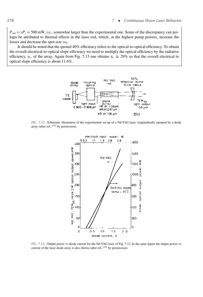
278 7 � Continuous Wave Laser Behavior
Pout D yPs D 500 mW, i.e., somewhat larger than the experimental one. Some of the discrepancy can per-haps be attributed to thermal effects in the laser rod, which, at the highest pump powers, increase thelosses and decrease the spot size w0.
It should be noted that the quoted 40% efficiency refers to the optical-to-optical efficiency. To obtainthe overall electrical-to-optical slope efficiency we need to multiply the optical efficiency by the radiativeefficiency, �r, of the array. Again from Fig. 7.13 one obtains �r Š 29% so that the overall electrical tooptical slope efficiency is about 11.6%.
FIG. 7.12. Schematic illustration of the experimental set-up of a Nd:YAG laser, longitudinally pumped by a diodearray (after ref.,.15/ by permission).
FIG. 7.13. Output power vs diode current for the Nd:YAG laser of Fig. 7.12. In the same figure the output power vscurrent of the laser diode array is also shown (after ref.,.15/ by permission).
7.4 � Threshold Condition and Output Power: Quasi-Three-Level Laser 279
7.4. THRESHOLD CONDITION AND OUTPUT POWER:QUASI-THREE-LEVEL LASER
We shall now investigate the threshold condition and output power for a quasi-three-levellaser. The laser behavior will first be considered within the space-independent rate-equationmodel of Sect. 7.2.2. The results predicted from the space-dependent model will then bediscussed and a comparison made between the two models.
7.4.1. Space-Independent Model
The analysis for a quasi-three-level laser proceeds in a similar way to that for a four-levelcase, starting now from Eqs. (7.2.24).
The threshold inversion is obtained by putting .d�=dt/ D 0 in Eq. (7.2.24b), thus giving
Nc D V
Va�ec�cD �
�el(7.4.1)
i.e., the same expression as for a four-level laser. The critical pump rate is then obtained fromEq. (7.2.24a) by setting .dN=dt/ D 0, � D 0, and N D Nc. We obtain
Rcp D fNt C Nc
.1 C f / �(7.4.2)
Since in most cases one has f � 1, one can write .1Cf / Š 1 in the denominator of Eq. (7.4.2).Comparison of Eq. (7.4.2) with Eq. (7.3.3) then shows that the critical pump rate for a quasi-three-level is increased over that for a four-level laser by the presence of the additional termfNt in the numerator of Eq. (7.4.2). In typical situations, this term may perhaps be � 5 timeslarger than Nc. For the case of uniform pumping by a diode laser, according to the discussionin Sect. 6.3.3, we can write Rp D �pPp=h�pAl where A is the cross sectional area of the activemedium and l its length. Using this expression in Eq. (7.4.2) we obtain the threshold pumppower as
Pth D h�p
�p�
.f Nt C Nc/Al
.1 C f /(7.4.3)
With the help of Eqs. (7.2.22) and (7.4.1), one can put Eq. (7.4.3) in the more suggestive form[compare with Eq. (7.3.12)]
Pth D �.1 C B/
�p
�h�p
�
� �A
�e C �a
�(7.4.4)
where we have set
B D �aNtl=� (7.4.5)
Above threshold, the c.w. inversion, N0, and the cw photon number, �0, are obtained fromEq. (7.2.24) by letting .dN=dt/ D .d�=dt/ D 0. Just as for the four-level laser, N0 is again
280 7 � Continuous Wave Laser Behavior
seen to be equal to Nc while �0, as obtained from Eq. (7.2.24a) with the help of Eq. (7.4.2), isgiven by
�0 D V
N0.�e C �a/c
f Nt C N0
�.x � 1/ (7.4.6)
where x D Rp=Rcp D Pp=Pth and again represents the amount by which threshold is exceeded.Equation (7.4.6), using Eq. (7.4.1) for N0 and with the help of Eqs. (7.2.14), (7.2.15)and (7.2.22), transforms to
�0 D�
Ab�.1 C B/
�e C �a
� ��c
�
�.x � 1/ (7.4.7)
where we have set Va D Abl, Ab being the beam area in the medium, which is assumed to besmaller than or equal to the cross-sectional area of the active medium.
The output power through e.g. mirror 2, is obtained from Eq. (7.2.18), using Eqs. (7.4.7)and (7.2.14), as [compare with Eq. (7.3.9)]
Pout D�
Ab.1 C B/
�e C �a
� �h�
�
� ��2
2
� � Pp
Pth� 1
�(7.4.8)
The laser slope efficiency, �s D .dPout=dPp/, is then readily obtained from Eq. (7.4.8) as
�s D�
Ab.1 C B/
�e C �a
� �h�
�
� ��2
2
� � 1
Pth
�(7.4.9)
With the help of Eqs. (7.4.4), (7.4.9) gives
�s D �p
��2
2�
� �h�
h�p
� �Ab
A
�(7.4.10)
Thus, given the same parameters, the slope efficiency of a quasi-three-level laser is predictedto be the same as that of a four level laser. At first sight this result might seem unexpectedowing to the increased loss, in a quasi-three-level laser, arising from ground state absorption.However, the energy removed via ground-state absorption actually raises atoms to the upperlaser level and these atoms are then available for producing stimulated emission.
7.4.2. Space-Dependent Model.16,17/
We now consider the case where the mode distribution and pump rate are assumed to bespatially dependent. We limit ourselves to a discussion of the most relevant results correspond-ing to the active medium being longitudinally pumped by a beam with Gaussian transverseprofile. We again refer to Appendix E for a more detailed treatment of this case as well as ofthe case of uniform pumping. We assume that the field intensity profile is again described byEq. (7.3.23) and the spatial distribution of the pump rate by (6.3.7) which is repeated here forconvenience
Rp.r, z/ D �r�t
�Pp
h�p
� 2˛
w2p
!exp
"�
2r2
w2p
!#exp .�˛ z/ (7.4.11)
7.4 � Threshold Condition and Output Power: Quasi-Three-Level Laser 281
As far as the threshold condition is concerned, one again finds that Eq. (7.4.1) still holds forthe average value of N i.e.,
<N>c D .�=�el/ (7.4.12)
where the average value is calculated according to Eq. (7.3.20). To obtain the thresholdpump rate we notice that, at each point of the active medium, below or at threshold, anequilibrium must exist between the number of atoms raised by the pumping process andthe number of atoms decaying spontaneously. Thus, from Eq. (7.2.24a), we obtain Rp DŒfNt C N.r, z/�=.1 C f /� . Upon averaging this expression over the mode intensity distributionand using the expression for threshold inversion given by Eq. (7.4.12) we obtain
<Rp>c D �aNtl C �
.�e C �a/l�(7.4.13)
If the pump rate expression Eq. (7.4.11) is substituted into the left hand side of Eq. (7.4.13)and if the average of Rp over the field intensity profile is calculated, we end up with thethreshold pump power expression of given by Eq. (6.3.25) which is repeated here in a slightlydifferent form [compare with Eq. (7.4.4)]
Pth D �.1 C B/
�p
�h�p
�
�" w2
0 C w2p
�2.�e C �a/
#(7.4.14)
where B is again given by Eq. (7.4.5).Above threshold, using the condition .d�=dt/ D 0, one again finds that the average gain
must equal losses, thus giving
<N>0 D<N>c D �=�el (7.4.15)
The calculation of output power is considered in some detail in Appendix E and we limitourselves here to quoting and discussing the final result. First, we define x as the factor bywhich threshold is exceeded as in Eq. (7.3.25) and a minimum threshold power Pmth as thethreshold value which holds for w0 � wp and B � 1 Œ�aNtl � ��. From Eq. (7.4.14) we get
Pmth D �
�p
�h�p
�
� " w2
p
2.�e C �a/
#(7.4.16)
We also define a normalized output power as in Eq. (7.3.27) where now
Ps D �2
2
� w2
0
2.�e C �a/
� �h�
�
�(7.4.17)
The relation between y and x then turns out to be
x D1 C B ln.1Cy/
yR 10
t˛dt1Cyt
(7.4.18)
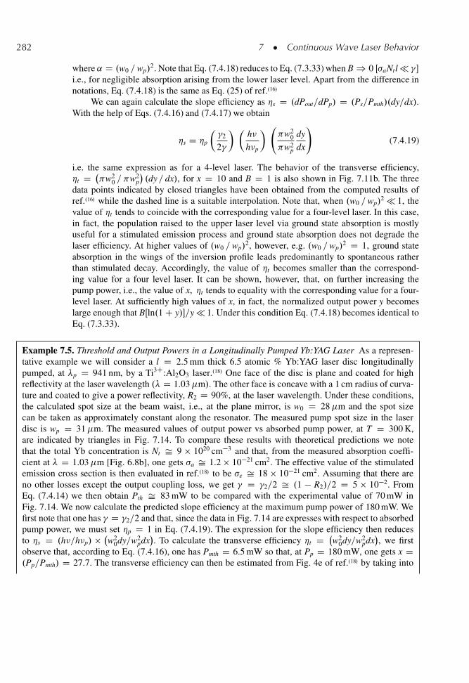
282 7 � Continuous Wave Laser Behavior
where ˛ D .w0 =wp/2. Note that Eq. (7.4.18) reduces to Eq. (7.3.33) when B ) 0 Œ�aNtl � ��
i.e., for negligible absorption arising from the lower laser level. Apart from the difference innotations, Eq. (7.4.18) is the same as Eq. (25) of ref..16/
We can again calculate the slope efficiency as �s D .dPout=dPp/ D .Ps=Pmth/.dy=dx/.With the help of Eqs. (7.4.16) and (7.4.17) we obtain
�s D �p
��2
2�
� �h�
h�p
� w2
0
w2p
dy
dx
!(7.4.19)
i.e. the same expression as for a 4-level laser. The behavior of the transverse efficiency,�t D
w20 = w2
p
�.dy = dx/, for x D 10 and B D 1 is also shown in Fig. 7.11b. The three
data points indicated by closed triangles have been obtained from the computed results ofref..16/ while the dashed line is a suitable interpolation. Note that, when .w0 =wp/
2 � 1, thevalue of �t tends to coincide with the corresponding value for a four-level laser. In this case,in fact, the population raised to the upper laser level via ground state absorption is mostlyuseful for a stimulated emission process and ground state absorption does not degrade thelaser efficiency. At higher values of .w0 =wp/
2, however, e.g. .w0 =wp/2 D 1, ground state
absorption in the wings of the inversion profile leads predominantly to spontaneous ratherthan stimulated decay. Accordingly, the value of �t becomes smaller than the correspond-ing value for a four level laser. It can be shown, however, that, on further increasing thepump power, i.e., the value of x, �t tends to equality with the corresponding value for a four-level laser. At sufficiently high values of x, in fact, the normalized output power y becomeslarge enough that BŒln.1 C y/�=y � 1. Under this condition Eq. (7.4.18) becomes identical toEq. (7.3.33).
Example 7.5. Threshold and Output Powers in a Longitudinally Pumped Yb:YAG Laser As a represen-tative example we will consider a l D 2.5 mm thick 6.5 atomic % Yb:YAG laser disc longitudinallypumped, at �p D 941 nm, by a Ti3C:Al2O3 laser..18/ One face of the disc is plane and coated for highreflectivity at the laser wavelength .� D 1.03�m/. The other face is concave with a 1 cm radius of curva-ture and coated to give a power reflectivity, R2 D 90%, at the laser wavelength. Under these conditions,the calculated spot size at the beam waist, i.e., at the plane mirror, is w0 D 28�m and the spot sizecan be taken as approximately constant along the resonator. The measured pump spot size in the laserdisc is wp D 31�m. The measured values of output power vs absorbed pump power, at T D 300 K,are indicated by triangles in Fig. 7.14. To compare these results with theoretical predictions we notethat the total Yb concentration is Nt Š 9 � 1020 cm�3 and that, from the measured absorption coeffi-cient at � D 1.03�m [Fig. 6.8b], one gets �a Š 1.2 � 10�21 cm2. The effective value of the stimulatedemission cross section is then evaluated in ref..18/ to be �e Š 18 � 10�21 cm2. Assuming that there areno other losses except the output coupling loss, we get � D �2=2 Š .1 � R2/=2 D 5 � 10�2. FromEq. (7.4.14) we then obtain Pth Š 83 mW to be compared with the experimental value of 70 mW inFig. 7.14. We now calculate the predicted slope efficiency at the maximum pump power of 180 mW. Wefirst note that one has � D �2=2 and that, since the data in Fig. 7.14 are expresses with respect to absorbedpump power, we must set �p D 1 in Eq. (7.4.19). The expression for the slope efficiency then reducesto �s D .h�=h�p/ �
w20dy=w2
pdx�. To calculate the transverse efficiency �t D
w20dy=w2
pdx�, we first
observe that, according to Eq. (7.4.16), one has Pmth D 6.5 mW so that, at Pp D 180 mW, one gets x D.Pp=Pmth/ D 27.7. The transverse efficiency can then be estimated from Fig. 4e of ref..18/ by taking into
7.5 � Optimum Output Coupling 283
account that �t D dS=dF, B D �aNtl=� Š 5, a D wp=w0 Š 1.1, .F=Fth/ D xa2=.1Ca2/.1CB/ Š 2.16,where the quantities S, F, and Fth are defined in the cited reference. We obtain �t D dS=dF Š 70% sothat �s D .h�=h�p/�t Š 63%. A more exact calculation of the output power vs pump power, as obtaineddirectly from Eq. (7.4.18), is also plotted as a solid line in Fig. 7.14. From this calculation one gets amore exact value of the predicted slope efficiency of �s D 59% at Pp D 180 mW, to be compared withthe value of 56% obtained from the four points in the figure corresponding to the highest experimentalpowers.
FIG. 7.14. Plots of the output power vs absorbed pump power for a Ti:sapphire-pumped Yb:YAG laser, for liquidnitrogen cooled operation (77 K) and at room temperature operation (300 K) (after ref.,.18/ by permission).
7.5. OPTIMUM OUTPUT COUPLING
For a fixed pump rate, there is some value for the transmission, T2, of the output mirrorthat maximizes the output power..19/ Physically, the reason for this optimum arises from thefact that, as T2 is increased, we have the following two contrasting circumstances: (1) Theoutput power tends to increase due to the increased mirror transmission. (2) The output powertends to decrease since the increased cavity losses cause the number of cavity photons, �0, todecrease
To find the optimum output coupling condition, we will limit ourselves to a four-levellaser and consider the space-independent model. The optimum transmission is then obtainedfrom Eq. (7.3.9) by imposing the condition dPout=d�2 D 0 for a fixed value of pump powerPp. We must obviously take into account the fact that, according to Eq. (7.3.12), Pth is also afunction of �2. From Eq. (7.3.12) one can then write
Pth D Pmth�
�i C .�1 = 2/(7.5.1)
where Pmth, the minimum threshold pump power, is the threshold pump power for zero outputcoupling, �2 D 0. Equation (7.3.9) can then be transformed to
Pout DhAbIs
��i C �1
2
�iS
�xm
S C 1� 1
�(7.5.2)
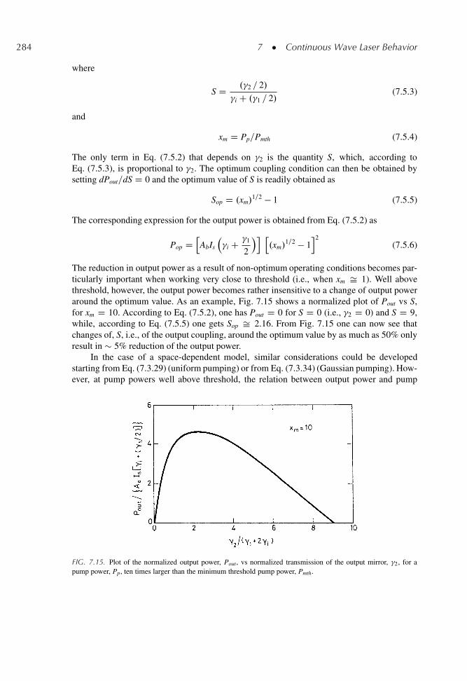
284 7 � Continuous Wave Laser Behavior
where
S D .�2 = 2/
�i C .�1 = 2/(7.5.3)
and
xm D Pp=Pmth (7.5.4)
The only term in Eq. (7.5.2) that depends on �2 is the quantity S, which, according toEq. (7.5.3), is proportional to �2. The optimum coupling condition can then be obtained bysetting dPout=dS D 0 and the optimum value of S is readily obtained as
Sop D .xm/1=2 � 1 (7.5.5)
The corresponding expression for the output power is obtained from Eq. (7.5.2) as
Pop DhAbIs
��i C �1
2
�i h.xm/
1=2 � 1i2
(7.5.6)
The reduction in output power as a result of non-optimum operating conditions becomes par-ticularly important when working very close to threshold (i.e., when xm Š 1). Well abovethreshold, however, the output power becomes rather insensitive to a change of output poweraround the optimum value. As an example, Fig. 7.15 shows a normalized plot of Pout vs S,for xm D 10. According to Eq. (7.5.2), one has Pout D 0 for S D 0 (i.e., �2 D 0) and S D 9,while, according to Eq. (7.5.5) one gets Sop Š 2.16. From Fig. 7.15 one can now see thatchanges of, S, i.e., of the output coupling, around the optimum value by as much as 50% onlyresult in � 5% reduction of the output power.
In the case of a space-dependent model, similar considerations could be developedstarting from Eq. (7.3.29) (uniform pumping) or from Eq. (7.3.34) (Gaussian pumping). How-ever, at pump powers well above threshold, the relation between output power and pump
FIG. 7.15. Plot of the normalized output power, Pout, vs normalized transmission of the output mirror, �2, for apump power, Pp, ten times larger than the minimum threshold pump power, Pmth.
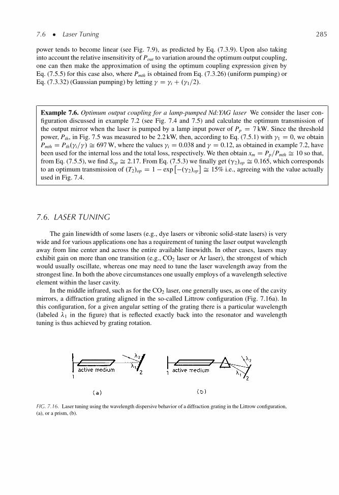
7.6 � Laser Tuning 285
power tends to become linear (see Fig. 7.9), as predicted by Eq. (7.3.9). Upon also takinginto account the relative insensitivity of Pout to variation around the optimum output coupling,one can then make the approximation of using the optimum coupling expression given byEq. (7.5.5) for this case also, where Pmth is obtained from Eq. (7.3.26) (uniform pumping) orEq. (7.3.32) (Gaussian pumping) by letting � D �i C .�1=2/.
Example 7.6. Optimum output coupling for a lamp-pumped Nd:YAG laser We consider the laser con-figuration discussed in example 7.2 (see Fig. 7.4 and 7.5) and calculate the optimum transmission ofthe output mirror when the laser is pumped by a lamp input power of Pp D 7 kW. Since the thresholdpower, Pth, in Fig. 7.5 was measured to be 2.2 kW, then, according to Eq. (7.5.1) with �1 D 0, we obtainPmth D Pth.�i=�/ Š 697 W, where the values �i D 0.038 and � D 0.12, as obtained in example 7.2, havebeen used for the internal loss and the total loss, respectively. We then obtain xm D Pp=Pmth Š 10 so that,from Eq. (7.5.5), we find Sop Š 2.17. From Eq. (7.5.3) we finally get .γ2/op Š 0.165, which correspondsto an optimum transmission of .T2/op D 1 � exp
��.γ2/op Š 15% i.e., agreeing with the value actually
used in Fig. 7.4.
7.6. LASER TUNING
The gain linewidth of some lasers (e.g., dye lasers or vibronic solid-state lasers) is verywide and for various applications one has a requirement of tuning the laser output wavelengthaway from line center and across the entire available linewidth. In other cases, lasers mayexhibit gain on more than one transition (e.g., CO2 laser or Ar laser), the strongest of whichwould usually oscillate, whereas one may need to tune the laser wavelength away from thestrongest line. In both the above circumstances one usually employs of a wavelength selectiveelement within the laser cavity.
In the middle infrared, such as for the CO2 laser, one generally uses, as one of the cavitymirrors, a diffraction grating aligned in the so-called Littrow configuration (Fig. 7.16a). Inthis configuration, for a given angular setting of the grating there is a particular wavelength(labeled �1 in the figure) that is reflected exactly back into the resonator and wavelengthtuning is thus achieved by grating rotation.
FIG. 7.16. Laser tuning using the wavelength dispersive behavior of a diffraction grating in the Littrow configuration,(a), or a prism, (b).
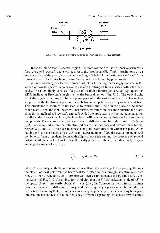
286 7 � Continuous Wave Laser Behavior
FIG. 7.17. Use of a birefringent filter as a wavelength-selective element.
In the visible or near IR spectral region, it is more common to use a dispersive prism withfaces close to Brewster’s angle with respect to the laser beam (Fig. 7.16b). Again, for a givenangular setting of the prism, a particular wavelength (labeled �1 in the figure) is reflected frommirror 2 exactly back into the resonator. Tuning is thus achieved by prism rotation.
A third wavelength-selective element, which is becoming increasingly popular in thevisible or near IR spectral region, makes use of a birefringent filter inserted within the lasercavity. The filter simply consists of a plate of a suitable birefringent crystal (e.g., quartz orKDP) inclined at Brewster’s angle, B, to the beam direction (Fig. 7.17). The optical axis,A, of the crystal is assumed to be in a plane parallel to the surface of the plate. Let us firstsuppose that the birefringent plate is placed between two polarizers with parallel orientation.This orientation is assumed to be such as to transmit the E-field in the plane of incidenceof the plate. Then, the input beam will not suffer any reflection loss upon entering the plate,since this is inclined at Brewster’s angle. Provided the optic axis is neither perpendicular norparallel to the plane of incidence, the input beam will contain both ordinary and extraordinarycomponents. These components will experience a difference in phase shifts � D 2 .ne �no/Le, where no and ne are the refractive indices for the ordinary and extraordinary beams,respectively, and Le is the plate thickness along the beam direction within the plate. Afterpassing through the plates, unless � is an integer number of 2 , the two components willcombine to form a resultant beam with elliptical polarization and the presence of secondpolarizer will then lead to loss for this elliptically polarized light. On the other hand, if � isan integral number of 2 , i.e., if
2
�.ne � no/Le D 2l (7.6.1)
where l is an integer, the beam polarization will remain unchanged after passing throughthe plate. For ideal polarizers the beam will then suffer no loss through the entire system ofFig. 7.17. For a general value of � one can then easily calculate the transmission, T, ofthe system of Fig. 7.17. Assuming, for simplicity, that the E-field makes an angle of 45ı tothe optical A-axis, one easily obtain T D cos2.� = 2/. Consecutive transmission maximahave their values of l differing by unity, and their frequency separation can be found fromEq. (7.6.1). Assuming that .ne �no/ does not change appreciably over the wavelength range ofinterest, one has the result that the frequency difference separating two consecutive maxima,
7.7 � Reasons for Multimode Oscillation 287
Example 7.7. Free spectral range and resolving powerof a birefringent filter Consider a dye laser operating atthe wavelength �D 600 nm in which a birefringent filterconsisting of a L D 1.5 mm thick potassium dihydrogenphosphate (KDP) crystal is inserted for laser tuning. Theordinary and extraordinary refractive indices, at the laserwavelength, are no D 1.47 and ne D 1.51. The Brewsterangle for this plate is B Š tan�1 n Š 56.13ı, where nhas been taken as the average of no and ne. The Brew-ster angle inside the crystal is then given by Snell’slaw as 0
B D 33.9ı so that Le D L= cos 0B Š 1.81 mm. If
the orientation of the optic axis A in Fig. 7.17 is nearorthogonal to the beam direction, the refractive indexof the extraordinary beam to be used in Eq. (7.6.2) isjust ne D 1.51, and from Eq. (7.6.2) one gets �fsr Š4.14 � 1012 Hz. The corresponding wavelength intervalbetween two consecutive peaks is �D�.�fsr=�/ Š5 nm, where �D c=�D 5�1014 Hz is the frequency of theradiation. Since the transmission of the birefringent filterof Fig. 7.17 is equal to T D cos2.�=2/, one can readilyshow that the width of the transmission curve (full widthbetween half-maximum points) is just equal to �=2 i.e.it is equal to � 2.5 nm.
i.e., the free spectral range,�fsr, isgiven by
�fsr D c0
.ne � no/Le(7.6.2)
Accordingly, the plate thickness, whichusually ranges between 0.3 and 1.5 mm,determines the width of the tuning curve andthus the resolving power. The thinner theplate, the greater the available tuning rangeand the lower the resolving power. Tuning ofone transmission peak can then be achievedupon rotating the plate around the normalto the surface. By doing so, in fact, onechanges the value of ne, which depends onthe angle between the optical axis and theelectric field vector, and hence changes theplate birefringencen D ne�no. Note finallythat, in low gain lasers such as cw gas or dyelasers, one can dispense with the two polar-izers if other polarizing element, such as theactive medium or indeed the Brewster’s anglesurfaces of the birefringent plate itself, pro-vide sufficient loss discrimination betweenthe two polarizations.
7.7. REASONS FOR MULTIMODE OSCILLATION
Lasers generally tend to oscillate on many modes. The reason for this behavior arisesessentially from the fact that the frequency separation of the modes is usually smaller, andoften very much smaller, than the width of the gain profile. If, for example, we take L D 1 m,the frequency difference between two consecutive longitudinal modes will be � D c=2L D150 MHz. The laser linewidth, on the other hand, may range from � 1 GHz, for a Dopplerbroadened transition of a visible or near IR gas laser, up to 300 GHz or more for a transitionof a crystal ion in a solid state material. The number of modes within the laser linewidthmay thus range from a few to a few thousands and the gain difference between these modes,particularly when a few thousand modes are considered, becomes very small. At first sightone would therefore expect a significant fraction of these modes to be excited at a sufficientlyhigh pump rate.
The above, seemingly straightforward, conclusion needs to be examined more carefully,however. In fact, in the early days of laser development, it was argued that in principle lasersshould always tend to oscillate on a single mode, provided the gain line was homogeneouslybroadened. The argument can be followed with the help of Fig. 7.18, in which the lasergain profile is plotted vs frequency for increasing values of the pump rate. For simplicity,
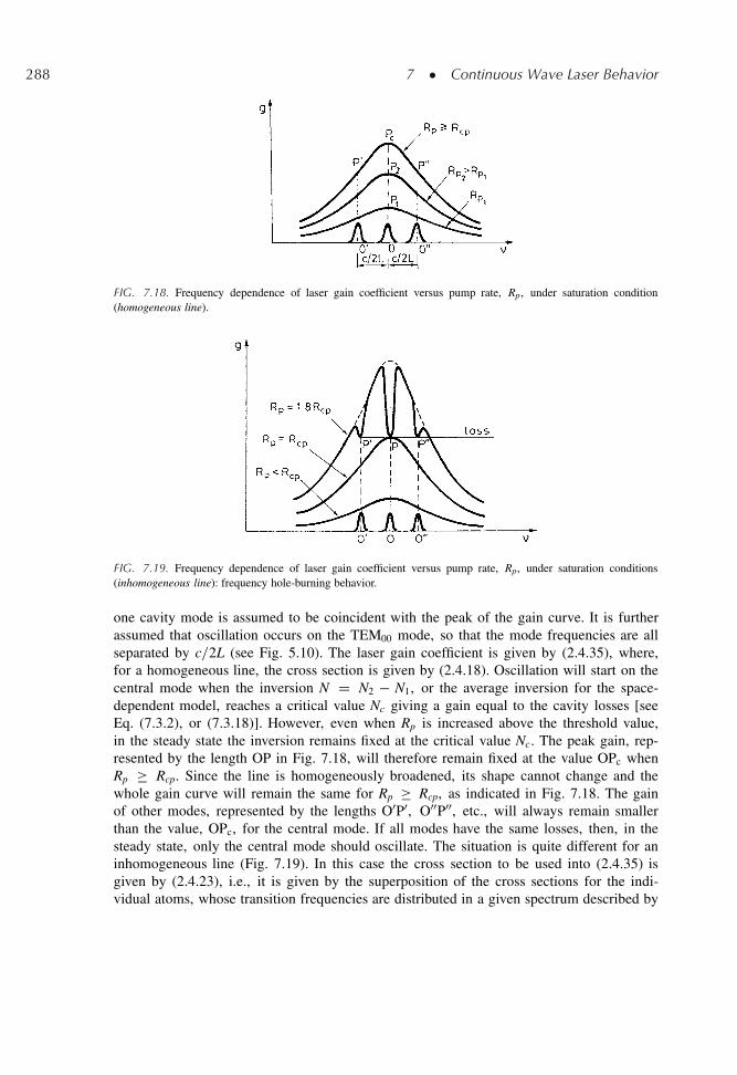
288 7 � Continuous Wave Laser Behavior
FIG. 7.18. Frequency dependence of laser gain coefficient versus pump rate, Rp, under saturation condition(homogeneous line).
FIG. 7.19. Frequency dependence of laser gain coefficient versus pump rate, Rp, under saturation conditions(inhomogeneous line): frequency hole-burning behavior.
one cavity mode is assumed to be coincident with the peak of the gain curve. It is furtherassumed that oscillation occurs on the TEM00 mode, so that the mode frequencies are allseparated by c=2L (see Fig. 5.10). The laser gain coefficient is given by (2.4.35), where,for a homogeneous line, the cross section is given by (2.4.18). Oscillation will start on thecentral mode when the inversion N D N2 � N1, or the average inversion for the space-dependent model, reaches a critical value Nc giving a gain equal to the cavity losses [seeEq. (7.3.2), or (7.3.18)]. However, even when Rp is increased above the threshold value,in the steady state the inversion remains fixed at the critical value Nc. The peak gain, rep-resented by the length OP in Fig. 7.18, will therefore remain fixed at the value OPc whenRp Rcp. Since the line is homogeneously broadened, its shape cannot change and thewhole gain curve will remain the same for Rp Rcp, as indicated in Fig. 7.18. The gainof other modes, represented by the lengths O0P0, O00P00, etc., will always remain smallerthan the value, OPc, for the central mode. If all modes have the same losses, then, in thesteady state, only the central mode should oscillate. The situation is quite different for aninhomogeneous line (Fig. 7.19). In this case the cross section to be used into (2.4.35) isgiven by (2.4.23), i.e., it is given by the superposition of the cross sections for the indi-vidual atoms, whose transition frequencies are distributed in a given spectrum described by
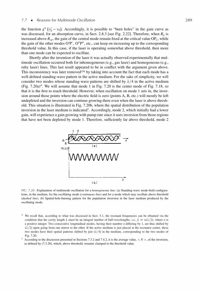
7.7 � Reasons for Multimode Oscillation 289
the function g� �00 � �0
�. Accordingly, it is possible to “burn holes” in the gain curve as
was discussed, for an absorption curve, in Sect. 2.8.3 [see Fig. 2.22]. Therefore, when Rp isincreased above Rcp, the gain of the central mode remain fixed at the critical value OPc, whilethe gain of the other modes O0P0, O00P00, etc., can keep on increasing up to the correspondingthreshold value. In this case, if the laser is operating somewhat above threshold, then morethan one mode can be expected to oscillate.
Shortly after the invention of the laser it was actually observed experimentally that mul-timode oscillation occurred both for inhomogeneous (e.g., gas laser) and homogeneous (e.g.,ruby laser) lines. This last result appeared to be in conflict with the argument given above.This inconsistency was later removed.20/ by taking into account the fact that each mode has awell-defined standing-wave pattern in the active medium. For the sake of simplicity, we willconsider two modes whose standing-wave patterns are shifted by �=4 in the active medium(Fig. 7.20a)�. We will assume that mode 1 in Fig. 7.20 is the center mode of Fig. 7.18, sothat it is the first to reach threshold. However, when oscillation on mode 1 sets in, the inver-sion around those points where the electric field is zero (points A, B, etc.) will mostly be leftundepleted and the inversion can continue growing there even when the laser is above thresh-old. This situation is illustrated in Fig. 7.20b, where the spatial distribution of the populationinversion in the laser medium is indicated�. Accordingly, mode 2, which initially had a lowergain, will experience a gain growing with pump rate since it uses inversion from those regionsthat have not been depleted by mode 1. Therefore, sufficiently far above threshold, mode 2
FIG. 7.20. Explanation of multimode oscillation for a homogeneous line: (a) Standing-wave mode-field configura-tions, in the medium, for the oscillating mode (continuous line) and for a mode which may oscillate above threshold(dashed line). (b) Spatial-hole-burning pattern for the population inversion in the laser medium produced by theoscillating mode.
� We recall that, according to what was discussed in Sect. 5.1, the resonant frequencies can be obtained via thecondition that the cavity length L must be an integral number of half-wavelengths, i.e., L D n.�=2/, where n isa positive integer. Two consecutive longitudinal modes, having their number n differing by 1, are thus shifted by.�=2/ upon going from one mirror to the other. If the active medium is just placed at the resonator center, thesetwo modes have their spatial patterns shifted by just .�=4/ in the medium, corresponding to the two modes ofFig. 7.20.
� According to the discussion presented in Sections 7.3.2 and 7.4.2, it is the average value, < N >, of the inversion,as defined by (7.3.20), which, above threshold, remains clamped to the threshold value.
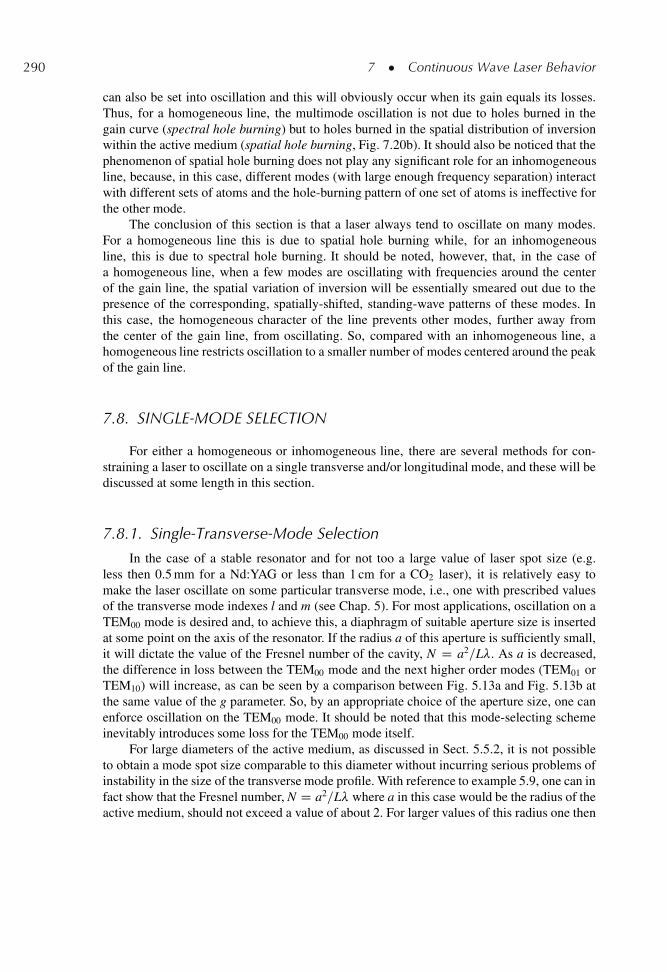
290 7 � Continuous Wave Laser Behavior
can also be set into oscillation and this will obviously occur when its gain equals its losses.Thus, for a homogeneous line, the multimode oscillation is not due to holes burned in thegain curve (spectral hole burning) but to holes burned in the spatial distribution of inversionwithin the active medium (spatial hole burning, Fig. 7.20b). It should also be noticed that thephenomenon of spatial hole burning does not play any significant role for an inhomogeneousline, because, in this case, different modes (with large enough frequency separation) interactwith different sets of atoms and the hole-burning pattern of one set of atoms is ineffective forthe other mode.
The conclusion of this section is that a laser always tend to oscillate on many modes.For a homogeneous line this is due to spatial hole burning while, for an inhomogeneousline, this is due to spectral hole burning. It should be noted, however, that, in the case ofa homogeneous line, when a few modes are oscillating with frequencies around the centerof the gain line, the spatial variation of inversion will be essentially smeared out due to thepresence of the corresponding, spatially-shifted, standing-wave patterns of these modes. Inthis case, the homogeneous character of the line prevents other modes, further away fromthe center of the gain line, from oscillating. So, compared with an inhomogeneous line, ahomogeneous line restricts oscillation to a smaller number of modes centered around the peakof the gain line.
7.8. SINGLE-MODE SELECTION
For either a homogeneous or inhomogeneous line, there are several methods for con-straining a laser to oscillate on a single transverse and/or longitudinal mode, and these will bediscussed at some length in this section.
7.8.1. Single-Transverse-Mode Selection
In the case of a stable resonator and for not too a large value of laser spot size (e.g.less then 0.5 mm for a Nd:YAG or less than 1 cm for a CO2 laser), it is relatively easy tomake the laser oscillate on some particular transverse mode, i.e., one with prescribed valuesof the transverse mode indexes l and m (see Chap. 5). For most applications, oscillation on aTEM00 mode is desired and, to achieve this, a diaphragm of suitable aperture size is insertedat some point on the axis of the resonator. If the radius a of this aperture is sufficiently small,it will dictate the value of the Fresnel number of the cavity, N D a2=L�. As a is decreased,the difference in loss between the TEM00 mode and the next higher order modes (TEM01 orTEM10) will increase, as can be seen by a comparison between Fig. 5.13a and Fig. 5.13b atthe same value of the g parameter. So, by an appropriate choice of the aperture size, one canenforce oscillation on the TEM00 mode. It should be noted that this mode-selecting schemeinevitably introduces some loss for the TEM00 mode itself.
For large diameters of the active medium, as discussed in Sect. 5.5.2, it is not possibleto obtain a mode spot size comparable to this diameter without incurring serious problems ofinstability in the size of the transverse mode profile. With reference to example 5.9, one can infact show that the Fresnel number, N D a2=L� where a in this case would be the radius of theactive medium, should not exceed a value of about 2. For larger values of this radius one then
7.8 � Single-Mode Selection 291
need to resort to unstable resonators. In particular, as discussed in Sect. 5.6.2, if the equivalentFresnel number is chosen to have a half-integer value, a large loss discrimination will occurbetween the lowest-order and the higher-order modes (see Fig. 5.20). In this case, the outputbeam is in the form of a ring, a shape which is not always convenient. The best way to obtainoscillation on the lowest-order mode, for this case, would then be to use an unstable cavitywith a radially variable output coupler of Gaussian or, even better, super-Gaussian profile(Sect. 5.6.4).
7.8.2. Single-Longitudinal-Mode Selection
Even when a laser is oscillating on a single transverse mode, it can still oscillate onseveral longitudinal modes (i.e., modes differing in their value of the longitudinal mode indexn). These modes are separated in frequency by � D c=2L. Isolation of a single longitudinalmode can be achieved, in some cases, by using such a short cavity length that � > �0=2,where � is the width of the gain curve�. In this case, if a mode is tuned to coincide with thecenter of the gain curve, the two adjacent longitudinal modes are far enough away from linecenter that, for a laser not too far above threshold, they cannot oscillate. The requirement forthis mode-selecting scheme can then be written as
L c= �0 (7.8.1)
So, for example, if the equality applies in Eq. (7.8.1) and if one mode is coincident withthe peak of the gain profile, the two adjacent modes will see an unsaturated gain coefficientthat, both for a Gaussian or Lorentzian line, is half that of the peak gain. In particular, for aGaussian line, one can easily understand from Fig. 7.19 that single longitudinal mode opera-tion is achieved for Rcp Rp 2Rcp. It should be noted that, to tune one mode to coincidencewith the line center, one needs to mount one cavity mirror on e.g. a piezo-electric transducer.Upon applying a voltage to this transducer, one can thereby produce a small controllablechange of the cavity length [one can show that the cavity length needs to be changed by �=2to shift the comb (Fig. 5.10 with l D m D 0) of the longitudinal modes by one mode spacing].
The method discussed above can be used effectively with a gas laser, notably with aHe-Ne laser, where gain linewidths are relatively small (a few GHz or smaller). For instance,in the case of a He-Ne laser oscillating on its red transition one has��
0 Š 1.7 GHz and fromEq. (7.8.1) we obtain L 17.5 cm. For solid-state-lasers, on the other hand, the gain linewidthis usually much larger (a few hundreds GHz) and, to fulfill Eq. (7.8.1), the equivalent cavitylength must typically be appreciably smaller than 1 mm (microchip-lasers). For lasers withmuch larger bandwidths (e.g., dye lasers or tunable solid-state lasers) the cavity length tofulfill Eq. (7.8.1) becomes too small to be practical. In this case and also when longer lengthsof the active medium are needed (e.g. for high power lasers), longitudinal mode selection canbe achieved by a variety of other techniques which are the subject of next two sections.
� If a tuning element, such as those in Figs. 7.16 and 7.17, is inserted in the laser cavity and if the correspondinglinewidth, ranging in actual cases between 0.1 nm 1 nm, is smaller than that of the gain medium, the linewidth �0
to be considered in this section is that of the tuning element rather than that of the active medium. Notably, thiscase occurs for dye lasers or for tunable solid-state lasers.
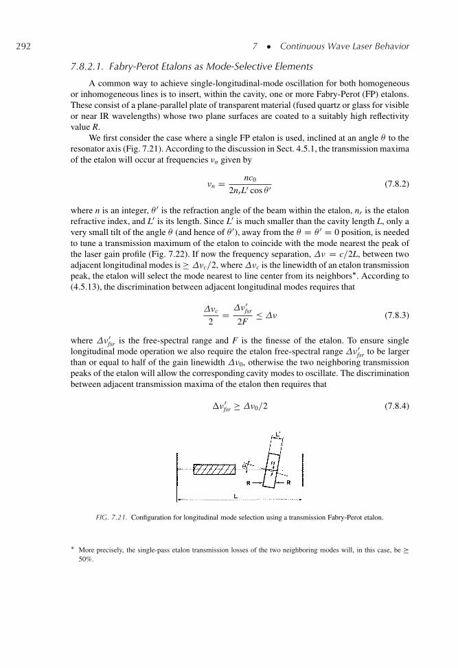
292 7 � Continuous Wave Laser Behavior
7.8.2.1. Fabry-Perot Etalons as Mode-Selective Elements
A common way to achieve single-longitudinal-mode oscillation for both homogeneousor inhomogeneous lines is to insert, within the cavity, one or more Fabry-Perot (FP) etalons.These consist of a plane-parallel plate of transparent material (fused quartz or glass for visibleor near IR wavelengths) whose two plane surfaces are coated to a suitably high reflectivityvalue R.
We first consider the case where a single FP etalon is used, inclined at an angle to theresonator axis (Fig. 7.21). According to the discussion in Sect. 4.5.1, the transmission maximaof the etalon will occur at frequencies �n given by
�n D nc0
2nrL0 cos 0 (7.8.2)
where n is an integer, 0 is the refraction angle of the beam within the etalon, nr is the etalonrefractive index, and L0 is its length. Since L0 is much smaller than the cavity length L, only avery small tilt of the angle (and hence of 0), away from the D 0 D 0 position, is neededto tune a transmission maximum of the etalon to coincide with the mode nearest the peak ofthe laser gain profile (Fig. 7.22). If now the frequency separation, � D c=2L, between twoadjacent longitudinal modes is �c=2, where�c is the linewidth of an etalon transmissionpeak, the etalon will select the mode nearest to line center from its neighbors�. According to(4.5.13), the discrimination between adjacent longitudinal modes requires that
�c
2D �0
fsr
2F � (7.8.3)
where �0fsr is the free-spectral range and F is the finesse of the etalon. To ensure single
longitudinal mode operation we also require the etalon free-spectral range �0fsr to be larger
than or equal to half of the gain linewidth �0, otherwise the two neighboring transmissionpeaks of the etalon will allow the corresponding cavity modes to oscillate. The discriminationbetween adjacent transmission maxima of the etalon then requires that
�� 0fsr �0=2 (7.8.4)
FIG. 7.21. Configuration for longitudinal mode selection using a transmission Fabry-Perot etalon.
� More precisely, the single-pass etalon transmission losses of the two neighboring modes will, in this case, be �50%.
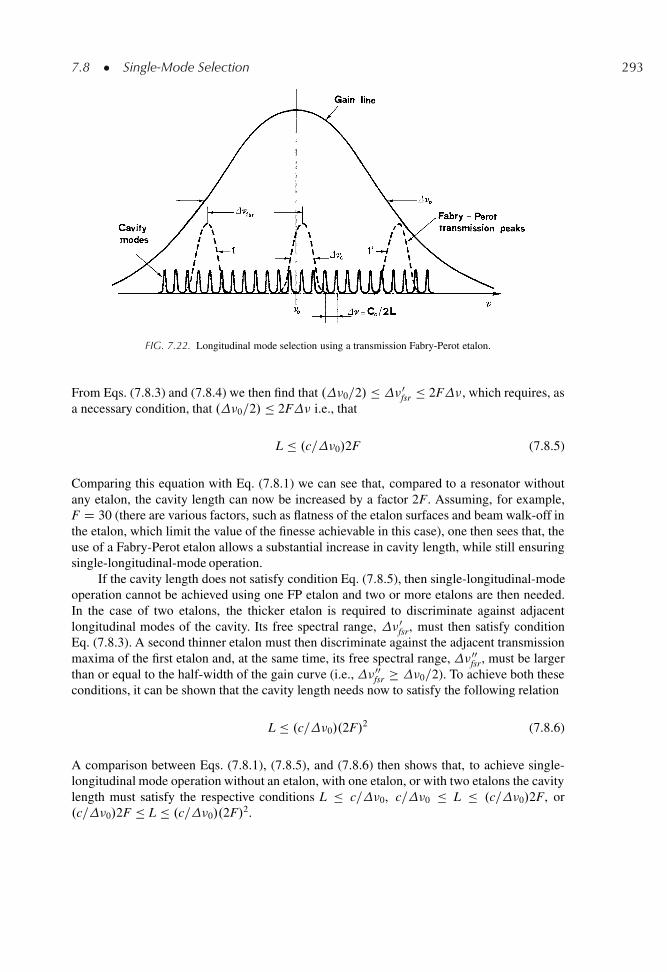
7.8 � Single-Mode Selection 293
FIG. 7.22. Longitudinal mode selection using a transmission Fabry-Perot etalon.
From Eqs. (7.8.3) and (7.8.4) we then find that .�0=2/ �0fsr 2F�, which requires, as
a necessary condition, that .�0=2/ 2F� i.e., that
L .c=�0/2F (7.8.5)
Comparing this equation with Eq. (7.8.1) we can see that, compared to a resonator withoutany etalon, the cavity length can now be increased by a factor 2F. Assuming, for example,F D 30 (there are various factors, such as flatness of the etalon surfaces and beam walk-off inthe etalon, which limit the value of the finesse achievable in this case), one then sees that, theuse of a Fabry-Perot etalon allows a substantial increase in cavity length, while still ensuringsingle-longitudinal-mode operation.
If the cavity length does not satisfy condition Eq. (7.8.5), then single-longitudinal-modeoperation cannot be achieved using one FP etalon and two or more etalons are then needed.In the case of two etalons, the thicker etalon is required to discriminate against adjacentlongitudinal modes of the cavity. Its free spectral range, � 0
fsr, must then satisfy conditionEq. (7.8.3). A second thinner etalon must then discriminate against the adjacent transmissionmaxima of the first etalon and, at the same time, its free spectral range, �00
fsr, must be largerthan or equal to the half-width of the gain curve (i.e., �00
fsr �0=2). To achieve both theseconditions, it can be shown that the cavity length needs now to satisfy the following relation
L .c=�0/.2F/2 (7.8.6)
A comparison between Eqs. (7.8.1), (7.8.5), and (7.8.6) then shows that, to achieve single-longitudinal mode operation without an etalon, with one etalon, or with two etalons the cavitylength must satisfy the respective conditions L c=�0, c=�0 L .c=�0/2F, or.c=�0/2F L .c=�0/.2F/2.
294 7 � Continuous Wave Laser Behavior
Example 7.8. Single-longitudinal-mode selection in an Ar and a Nd:YAG laser Consider first an Ar laseroscillating on its � D 514.5 nm line whose gain line-width has been experimentally measured to be��
0 D 3.5 GHz. To achieve single longitudinal mode selection without any etalon one would require acavity length L c=��
0 Š 8.6 cm; with one etalon, the cavity length needs to be L .c=��0 /.2F/ Š
5.14 m, where a finesse F D 30 has been used. Since the length of an Ar laser is usually smaller than2 m but larger than a few tens of cm, one FP etalon is required. According to Eq. (7.8.2), for cos 0 Š 1one has �0
fsr Š c=2nrL0, and, taking nr D 1.5, we get from Eq. (7.8.3) L0 L=2Fnr D 1.66 cm, wherea cavity length of L D 1.5 m has been considered. From Eq. (7.8.4), on the other hand, we obtain L0 .c=��
0 nr/ D 5.71 cm. The thickness of the etalon can then be chosen somewhere between these twovalues e.g. L0 D 3.7 cm. Consider now the case of a Nd:YAG laser for which one has �0 D 120 GHz(at T D 300 K). Single-longitudinal-mode oscillation without any etalon requires, in this case, a cavitylength L .c=�0n/ D 1.4 mm, where the refractive index of YAG is n D 1.82 (the two end mirrorsare assumed, in this case, to be directly coated on the two faces of the YAG plate so that the separationbetween two consecutive longitudinal modes is now given by � D c=2nL). Indeed, diode pumpedNd:YAG platelets with thickness of the order of a few hundred micrometers are now commonly usedand even commercially available (microchip lasers). When a single FP etalon is used, then, according toEq. (7.8.5) the cavity length can be increased up to L Š 9.5 cm (assuming again F D 30).
7.8.2.2. Single Mode Selection via Unidirectional Ring Resonators
For a homogeneously broadened transition, single-longitudinal mode operation can auto-matically be achieved, or at least greatly facilitated, if the laser cavity is in the form of a ringand oscillation is constrained to be unidirectional (see Fig. 5.4a). In this case, in fact, the phe-nomenon of spatial hole burning within the active medium does not occur and, as discussedin Sect. 7.7, the laser tends to oscillate on a single mode. Actually, if the transition is onlypartly homogeneously broadened and particularly when the gain profile is very broad, somefurther bandwidth selecting elements such as birefringent filters and/or Fabry-Perot etalonsmay also be needed. An additional advantage of this unidirectional ring configuration is thathigher output power is available since the whole of the active material rather than just thoseregions around the maxima of the standing-wave pattern contributes to the laser output.
To achieve unidirectional ring operation, a unidirectional device or optical diode, givingpreferential transmission for one direction of beam propagation, needs to be inserted withinthe cavity. In principle the device can be made as shown in Fig. 7.23. Here the wave goingin one direction, e.g., from left to right, passes first through an input polarizer (polarizer 1),then through a rod of suitable transparent material (e.g., glass) to which a longitudinal dcmagnetic field is applied (Faraday rotator), and then through an output polarizer (polarizer 2)which has the same orientation as the first polarizer�. When a linearly polarized optical beampasses through the Faraday rotator with beam axis along the magnetic field direction, the out-put beam still consists of a linearly polarized wave whose plane of polarization is howeverrotated about the beam axis. The sense of rotation, seen by an observer facing the oncomingbeam, depends on the relative direction of magnetic field and beam propagation direction.
� To avoid confusion and have a consistent way of describing the sense of a rotation of polarization, we will alwaysassume that the observer is facing the oncoming light beam.
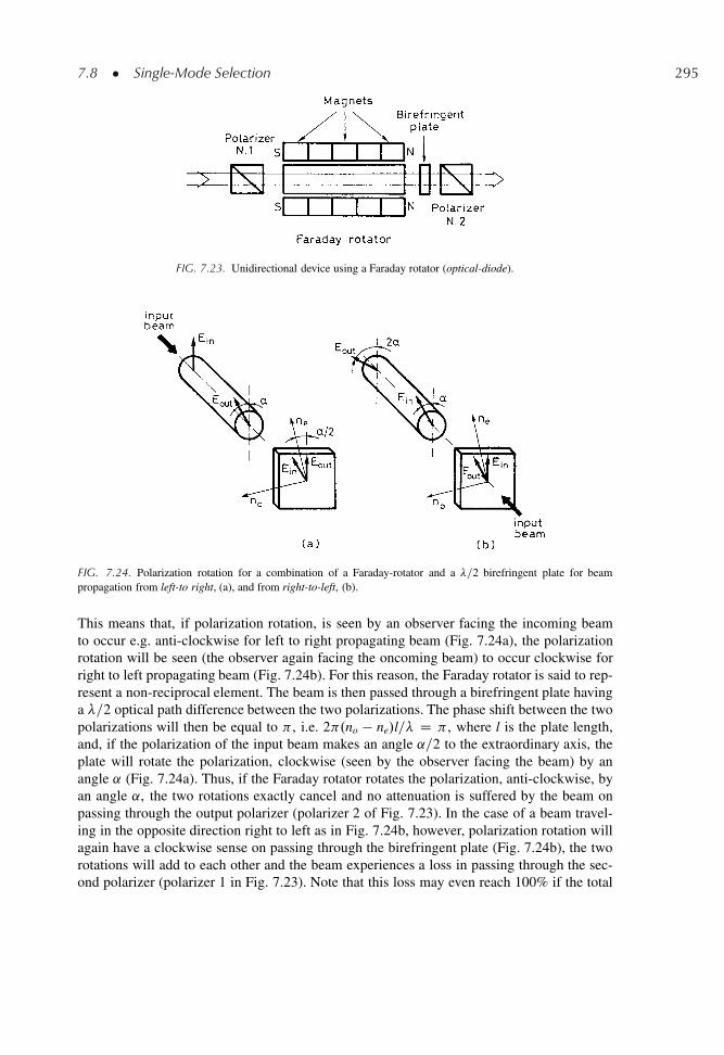
7.8 � Single-Mode Selection 295
FIG. 7.23. Unidirectional device using a Faraday rotator (optical-diode).
FIG. 7.24. Polarization rotation for a combination of a Faraday-rotator and a �=2 birefringent plate for beampropagation from left-to right, (a), and from right-to-left, (b).
This means that, if polarization rotation, is seen by an observer facing the incoming beamto occur e.g. anti-clockwise for left to right propagating beam (Fig. 7.24a), the polarizationrotation will be seen (the observer again facing the oncoming beam) to occur clockwise forright to left propagating beam (Fig. 7.24b). For this reason, the Faraday rotator is said to rep-resent a non-reciprocal element. The beam is then passed through a birefringent plate havinga �=2 optical path difference between the two polarizations. The phase shift between the twopolarizations will then be equal to , i.e. 2 .no � ne/l=� D , where l is the plate length,and, if the polarization of the input beam makes an angle ˛=2 to the extraordinary axis, theplate will rotate the polarization, clockwise (seen by the observer facing the beam) by anangle ˛ (Fig. 7.24a). Thus, if the Faraday rotator rotates the polarization, anti-clockwise, byan angle ˛, the two rotations exactly cancel and no attenuation is suffered by the beam onpassing through the output polarizer (polarizer 2 of Fig. 7.23). In the case of a beam travel-ing in the opposite direction right to left as in Fig. 7.24b, however, polarization rotation willagain have a clockwise sense on passing through the birefringent plate (Fig. 7.24b), the tworotations will add to each other and the beam experiences a loss in passing through the sec-ond polarizer (polarizer 1 in Fig. 7.23). Note that this loss may even reach 100% if the total
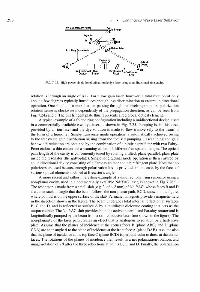
296 7 � Continuous Wave Laser Behavior
FIG. 7.25. High-power single-longitudinal mode dye laser using a unidirectional ring cavity.
rotation is through an angle of =2. For a low gain laser, however, a total rotation of onlyabout a few degrees typically introduces enough loss discrimination to ensure unidirectionaloperation. One should also note that, on passing through the birefringent plate, polarizationrotation sense is clockwise independently of the propagation direction, as can be seen fromFig. 7.24a and b. The birefringent plate thus represents a reciprocal optical element.
A typical example of a folded ring configuration including a unidirectional device, usedin a commercially available c.w. dye laser, is shown in Fig. 7.25. Pumping is, in this case,provided by an ion laser and the dye solution is made to flow transversely to the beam inthe form of a liquid jet. Single-transverse mode operation is automatically achieved owingto the transverse gain distribution arising from the focused pumping. Laser tuning and gainbandwidth reduction are obtained by the combination of a birefringent filter with two Fabry-Perot etalons, a thin etalon and a scanning etalon, of different free spectral ranges. The opticalpath length of the cavity is conveniently tuned by rotating a tilted, plane-parallel, glass plateinside the resonator (the galvoplate). Single longitudinal mode operation is then ensured byan unidirectional device consisting of a Faraday rotator and a birefringent plate. Note that nopolarizers are used because enough polarization loss is provided, in this case, by the faces ofvarious optical elements inclined at Brewster’s angle.
A more recent and rather interesting example of a unidirectional ring resonator using anon-planar cavity, used in a commercially available Nd:YAG laser, is shown in Fig 7.26..21/
The resonator is made from a small slab (e.g. 3 �6 �8 mm) of Nd:YAG, whose faces B and Dare cut at such an angle that the beam follows the non-planar path, BCD, shown in the figure,where point C is on the upper surface of the slab. Permanent magnets provide a magnetic fieldin the direction shown in the figure. The beam undergoes total internal reflection at surfacesB, C and D, and is reflected at surface A by a multilayer dielectric coating that acts as theoutput coupler. The Nd:YAG slab provides both the active material and Faraday rotator and islongitudinally pumped by the beam from a semiconductor laser (not shown in the figure). Thenon-planarity of the laser path creates an effect that is analogous to rotation by a half-waveplate. Assume that the planes of incidence at the corner faces B (plane ABC) and D (planeCDA) are at an angle ˇ to the plane of incidence at the front face A (plane DAB). Assume alsothat the plane of incidence at the top face C (plane BCD) is perpendicular to those at the cornerfaces. The rotations of the planes of incidence then result in a net polarization-rotation, andimage-rotation of 2ˇ after the three reflections at points B, C, and D. Finally, the polarization
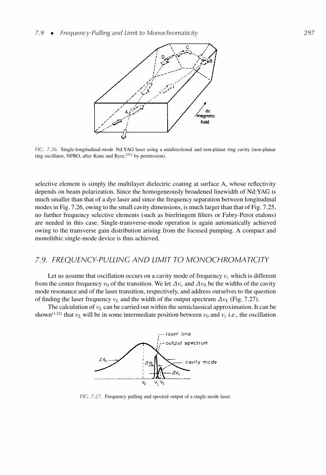
7.9 � Frequency-Pulling and Limit to Monochromaticity 297
FIG. 7.26. Single-longitudinal-mode Nd:YAG laser using a unidirectional and non-planar ring cavity (non-planarring oscillator, NPRO, after Kane and Byer,.21/ by permission).
selective element is simply the multilayer dielectric coating at surface A, whose reflectivitydepends on beam polarization. Since the homogeneously broadened linewidth of Nd:YAG ismuch smaller than that of a dye laser and since the frequency separation between longitudinalmodes in Fig. 7.26, owing to the small cavity dimensions, is much larger than that of Fig. 7.25,no further frequency selective elements (such as birefringent filters or Fabry-Perot etalons)are needed in this case. Single-transverse-mode operation is again automatically achievedowing to the transverse gain distribution arising from the focused pumping. A compact andmonolithic single-mode device is thus achieved.
7.9. FREQUENCY-PULLING AND LIMIT TO MONOCHROMATICITY
Let us assume that oscillation occurs on a cavity mode of frequency �c which is differentfrom the center frequency �0 of the transition. We let�c and�0 be the widths of the cavitymode resonance and of the laser transition, respectively, and address ourselves to the questionof finding the laser frequency �L and the width of the output spectrum �L (Fig. 7.27).
The calculation of �L can be carried out within the semiclassical approximation. It can beshown.3,22/ that �L will be in some intermediate position between �0 and �c i.e., the oscillation
FIG. 7.27. Frequency pulling and spectral output of a single mode laser.
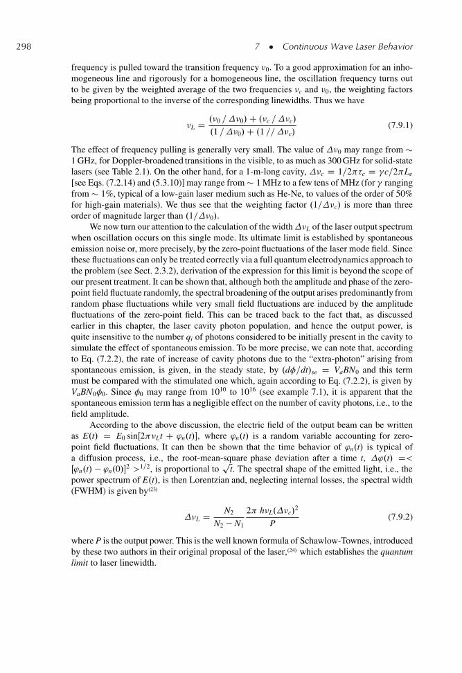
298 7 � Continuous Wave Laser Behavior
frequency is pulled toward the transition frequency �0. To a good approximation for an inho-mogeneous line and rigorously for a homogeneous line, the oscillation frequency turns outto be given by the weighted average of the two frequencies �c and �0, the weighting factorsbeing proportional to the inverse of the corresponding linewidths. Thus we have
�L D .�0 =�0/C .�c =�c/
.1 =�0/C .1 ==�c/(7.9.1)
The effect of frequency pulling is generally very small. The value of �0 may range from �1 GHz, for Doppler-broadened transitions in the visible, to as much as 300 GHz for solid-statelasers (see Table 2.1). On the other hand, for a 1-m-long cavity, �c D 1=2 �c D �c=2 Le
[see Eqs. (7.2.14) and (5.3.10)] may range from � 1 MHz to a few tens of MHz (for � rangingfrom � 1%, typical of a low-gain laser medium such as He-Ne, to values of the order of 50%for high-gain materials). We thus see that the weighting factor .1=�c/ is more than threeorder of magnitude larger than .1=�0/.
We now turn our attention to the calculation of the width�L of the laser output spectrumwhen oscillation occurs on this single mode. Its ultimate limit is established by spontaneousemission noise or, more precisely, by the zero-point fluctuations of the laser mode field. Sincethese fluctuations can only be treated correctly via a full quantum electrodynamics approach tothe problem (see Sect. 2.3.2), derivation of the expression for this limit is beyond the scope ofour present treatment. It can be shown that, although both the amplitude and phase of the zero-point field fluctuate randomly, the spectral broadening of the output arises predominantly fromrandom phase fluctuations while very small field fluctuations are induced by the amplitudefluctuations of the zero-point field. This can be traced back to the fact that, as discussedearlier in this chapter, the laser cavity photon population, and hence the output power, isquite insensitive to the number qi of photons considered to be initially present in the cavity tosimulate the effect of spontaneous emission. To be more precise, we can note that, accordingto Eq. (7.2.2), the rate of increase of cavity photons due to the “extra-photon” arising fromspontaneous emission, is given, in the steady state, by .d�=dt/se D VaBN0 and this termmust be compared with the stimulated one which, again according to Eq. (7.2.2), is given byVaBN0�0. Since �0 may range from 1010 to 1016 (see example 7.1), it is apparent that thespontaneous emission term has a negligible effect on the number of cavity photons, i.e., to thefield amplitude.
According to the above discussion, the electric field of the output beam can be writtenas E.t/ D E0 sinŒ2 �Lt C 'n.t/�, where 'n.t/ is a random variable accounting for zero-point field fluctuations. It can then be shown that the time behavior of 'n.t/ is typical ofa diffusion process, i.e., the root-mean-square phase deviation after a time t, '.t/ D<Œ'n.t/ � 'n.0/�2 >1=2, is proportional to
pt. The spectral shape of the emitted light, i.e., the
power spectrum of E.t/, is then Lorentzian and, neglecting internal losses, the spectral width(FWHM) is given by.23/
�L D N2
N2 � N1
2 h�L.�c/2
P(7.9.2)
where P is the output power. This is the well known formula of Schawlow-Townes, introducedby these two authors in their original proposal of the laser,.24/ which establishes the quantumlimit to laser linewidth.
7.9 � Frequency-Pulling and Limit to Monochromaticity 299
Example 7.9. Limit to laser linewidth in He-Ne andGaAs semiconductor lasers Consider first the case ofa single-mode He-Ne laser oscillating on its red tran-sition .�D 632.8 nm, �0 Š 4.7 � 1014 Hz/. We willtake Le D 1 m, � D 1% and we also assume an outputpower of P D 1 mW. From Eqs. (7.2.14) and (5.3.10)we get respectively �c D 3.3 � 10�7 s and �c Š 4.7 �105 Hz. From Eq. (7.9.2), taking N2=.N2 � N1/ Š 1,we obtain �L Š 0.43 mHz. Consider next the case ofa single-mode GaAs semiconductor laser .�D 850 nm/with a cavity length L D l D 300�m and with a powerreflectivity at the two end faces of R D 0.3 (i.e. equalto the Fresnel losses of the uncoated semiconductorsurfaces). Neglecting all other cavity losses we get� D � ln.R/ Š 1.03 and hence �c D nL=c� D 3.4 ps,where n D 3.5 is the refractive index of GaAs. We thenget ��c D 1=2 �c Š 4.7 � 1010 Hz and, from Eq. (7.9.2)assuming N2=.N2 � N1/D 3 and P D 3 mW, we obtain�L Š 3.2 MHz. Note that the laser linewidth is, in thiscase, almost 10 orders of magnitude larger than in thecase of a He-Ne laser on account of the much shortercavity decay time and hence of the much larger cavitylinewidth.
Typically, the linewidth predicted byEq. (7.9.2) turns out to be negligibly smallcompared to that produced by various othercavity disturbances, to be discussed lateron, except for the very important case ofa semiconductor laser. The reasons for thisexception are that, as shown in the follow-ing example,�c for a semiconductor laser istypically about 5 orders of magnitude largerthan that of e.g. a He-Ne laser. In fact, carefulexperiments done with GaAs lasers showedthe actual linewidth to be about 50–100 timeslarger than the value predicted by Eq. (7.9.2).This observation was later on understoodin terms of a new phenomenon peculiar ofa semiconductor laser. The fluctuations ofelectron-hole density caused by spontaneousemission produce, in fact, a measurable fluc-tuation of the refractive index of the lasermedium. The resulting fluctuation in opticalcavity length thereby produces a fluctuationof the cavity frequency and hence of theoscillation frequency. Thus, in a semiconduc-tor laser, the right hand side of Eq. (7.9.2)must be multiplied by a factor that we shalldenote as ˛2 and which is considerably larger than 1. The factor ˛ is called the Henry-factor,named after the scientist who first provided an explanation of this phenomenon..25/
According to the above example, the linewidth of a typical semiconductor laser arisesfrom quantum noise and, in practice, is difficult to reducing below 1 MHz. In the case of aHe-Ne laser and for all other lasers of relevance for obtaining small oscillation linewidths(such as Nd:YAG, CO2 or Ar lasers), the linewidth determined by the Schawlow-Townesformula, even for modest powers of a few mW, is always well below 1 Hz and down to themHz. Since �L D c=� Š 4.7 � 1014 Hz, the relative monochromaticity of this laser, set byzero-point fluctuations, would be .�L=�L/ Š 2.7 � 10�18. Now, let us examine the cavitylength stability requirement to keep the resonator frequency stable to the same degree. FromEq. (5.1.2) with n D const., we find .L=L/ Š �.�c=�c/ Š 2.7 � 10�18 so that, e.g., withL D 1 m, we have jLj Š 2.7 � 10�9 nm. This means that a cavity length variation by aquantity � 10�8 smaller than a typical atomic dimension is already enough to induce a shiftof the cavity frequency �c and hence of the oscillation frequency �L that is comparable to theoscillation linewidth given by Eq. (7.9.2). Thus, the limit to monochromaticity is, in practice,set by changes of cavity length induced by vibrations or thermal drifts, as we shall see in nextsection. These changes, arising from noise disturbances of perhaps less fundamental naturethan those considered above, are often said to be due to technical noise.
300 7 � Continuous Wave Laser Behavior
7.10. LASER FREQUENCY FLUCTUATIONS AND FREQUENCYSTABILIZATION
To consider laser frequency fluctuations, let us consider an active medium of refractiveindex nm and length l in a laser cavity of length L in air. The effective cavity length is thengiven by Le D na.L � l/ C nml, where na is the refractive index of air. We can then separatethe mode frequency changes into two parts: (i) Long-term drifts, i.e. occurring in a timelonger than, say, 1 s, of either L or na which are mainly caused by temperature drifts or slowpressure changes of the ambient air surrounding the laser. (ii) Short-term fluctuations causede.g. by acoustic vibrations of mirrors leading to cavity-length changes, by acoustic pressurewaves which modulate na, or by short-term fluctuations of nm, due e.g., to fluctuations of thedischarge current in a gas laser or to air bubbles in the jet flow of a dye laser. In opticallypumped solid-state lasers, fluctuations in pump power cause temperature fluctuations whichin turn change the refractive index and therefore the optical length of the cavity.
Example 7.10. Long term drift of a laser cavity Taking,for invar, ˛ D 1 � 10�6 K�1 and considering a frequencyin the central part of the visible spectrum, i.e. �L Š5 �1014 Hz, from the previous expressions we obtain thatthe frequency drift, �L, due to a thermal change, T,amounts to j�Lj D �L˛T D .5 � 108 T/ Hz. Thisshows that a change of T of, e.g., only 0.1 K wouldproduce a frequency drift of � 50 MHz. To calculate thefrequency drift due to a slow pressure change, we notethat, for a gas laser, one typically has .L � l/=Le Š 0.2while for air one has na Š 1.00027. Again for �L Š 5 �1014 Hz, we can then write j�Lj Š 2.7 � 1010jp=pjHz.Thus, for a relative pressure change jp=pj Š 3 � 10�3,which can readily occur during one hour time, one hasj�Lj Š 80 MHz.
To illustrate the influence of long-termdrifts on cavity length, let ˛ be the ther-mal expansion coefficient of the elements(e.g. invar rods) which determine the mir-ror separation. We then have j�L=�Lj ŠjL=Lj D ˛T, where T is the tempera-ture change of the laser environment. Slowpressure changes, on the other hand, con-tribute to the frequency drift by an amountj�Lj D �Ljnaj.L � l/=Le D �L.na �1/jp=pj.L � l/=Le, wherena is the changeof refractive index of the air as arising fromthe the slow change, p, of the ambientpressure, p.
According to the previous example, toreduce long-term frequency drifts below e.g.,1 MHz one needs to use very low expansion
materials for the spacer elements, down to an expansion coefficient perhaps smaller than1 � 10�7 K�1 and to stabilize the ambient temperature below 0.01 ıC. One also needs toenclose the laser in a pressure stabilized chamber. The reduction of short-term frequencyfluctuations is an even more difficult problem and one needs to rely on good vibration isolationoptical tables and efficient covers of the whole laser path. It is therefore generally difficult toreduce short term frequency fluctuations below the 1 MHz level, except for monolithic andcompact solid-state lasers, such as the NPRO laser considered in Fig. 7.26, where short-termfrequency fluctuations of about 10 kHz have been measured.
To characterize the spectrum of laser frequency fluctuations, let us write the electric fieldof the output beam as E.t/D E0 sinŒ2 �Lt C'n.t/� where �L is the central laser frequency and'n.t/ describes the noise phase fluctuations. The instantaneous frequency can then be writ-ten as �.t/ D �L C d'n.t/=2 dt D �L C �n.t/, where �n.t/ is the frequency noise. It is thisfrequency noise that is fundamentally related to linewidth or frequency stability, and, conse-quently, it is the term that needs to be characterized. The measure that is used to characterize
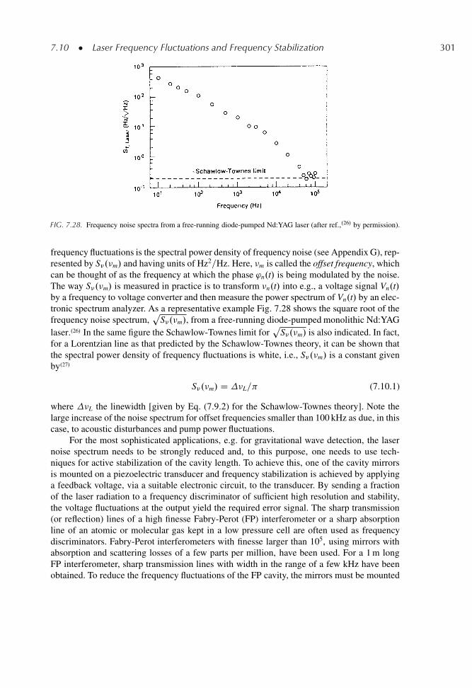
7.10 � Laser Frequency Fluctuations and Frequency Stabilization 301
FIG. 7.28. Frequency noise spectra from a free-running diode-pumped Nd:YAG laser (after ref.,.26/ by permission).
frequency fluctuations is the spectral power density of frequency noise (see Appendix G), rep-resented by S�.�m/ and having units of Hz2=Hz. Here, �m is called the offset frequency, whichcan be thought of as the frequency at which the phase 'n.t/ is being modulated by the noise.The way S�.�m/ is measured in practice is to transform �n.t/ into e.g., a voltage signal Vn.t/by a frequency to voltage converter and then measure the power spectrum of Vn.t/ by an elec-tronic spectrum analyzer. As a representative example Fig. 7.28 shows the square root of thefrequency noise spectrum,
pS�.�m/, from a free-running diode-pumped monolithic Nd:YAG
laser..26/ In the same figure the Schawlow-Townes limit forp
S�.�m/ is also indicated. In fact,for a Lorentzian line as that predicted by the Schawlow-Townes theory, it can be shown thatthe spectral power density of frequency fluctuations is white, i.e., S�.�m/ is a constant givenby.27/
S�.�m/ D �L= (7.10.1)
where �L the linewidth [given by Eq. (7.9.2) for the Schawlow-Townes theory]. Note thelarge increase of the noise spectrum for offset frequencies smaller than 100 kHz as due, in thiscase, to acoustic disturbances and pump power fluctuations.
For the most sophisticated applications, e.g. for gravitational wave detection, the lasernoise spectrum needs to be strongly reduced and, to this purpose, one needs to use tech-niques for active stabilization of the cavity length. To achieve this, one of the cavity mirrorsis mounted on a piezoelectric transducer and frequency stabilization is achieved by applyinga feedback voltage, via a suitable electronic circuit, to the transducer. By sending a fractionof the laser radiation to a frequency discriminator of sufficient high resolution and stability,the voltage fluctuations at the output yield the required error signal. The sharp transmission(or reflection) lines of a high finesse Fabry-Perot (FP) interferometer or a sharp absorptionline of an atomic or molecular gas kept in a low pressure cell are often used as frequencydiscriminators. Fabry-Perot interferometers with finesse larger than 105, using mirrors withabsorption and scattering losses of a few parts per million, have been used. For a 1 m longFP interferometer, sharp transmission lines with width in the range of a few kHz have beenobtained. To reduce the frequency fluctuations of the FP cavity, the mirrors must be mounted
302 7 � Continuous Wave Laser Behavior
using very low expansion elements (such as a tube made of super-invar or of very-low expan-sion ceramic) and the interferometer must be placed in a container providing pressure andtemperature control. Long term and absolute frequency stabilization can, however, only beachieved by using an atomic or molecular absorption line as a frequency reference. A goodreference wavelength should be reproducible and essentially independent of external pertur-bations such as electric or magnetic fields and temperature or pressure changes. Thereforetransitions in atoms or molecules without permanent dipole moments, such as CH4 for the3.39�m transition or 129I2 for the 633 nm transition of the He-Ne laser, are the most suitable.For a low pressure gas or vapor, the absorption line is limited, by Doppler broadening, to awidth of � 1 GHz (in the visible range). To obtain much narrower linewidths down perhapsto the kHz range, some kind of Doppler-free non-linear spectroscopy needs to be used..28/
A common method of frequency stabilization relies on the Pound-Drever technique.29/
where a small fraction of the output beam is frequency modulated and then passed throughthe frequency discriminator, i.e. the FP interferometer or the absorption cell. To understand theprinciple of operation of this technique, we need first to point out that, any element exhibitinga transmission which changes with frequency will also induce, on the incident wave, a phase-shift which depends on the wave frequency. For a FP interferometer used in transmission, thephase shift can be obtained from (4.5.4). For an absorption line, on the other hand, the phaseshift can be written as � D 2 nl=�, where l is the length of the absorption cell and n is therefractive index of the medium. For a Lorentzian line, the refractive index n can be related tothe absorption coefficient, ˛, of the medium by the dispersion relation
n.� � �0/ D 1 C c
2 �
�0 � ��0
˛.� � �0/ (7.10.2)
where n0 is the refractive index sufficiently far away from the resonance line, � is thefrequency of the e.m. wave, �0 is the transition frequency, and �0 is the transition width.Note that, for � D �0, one has n D n0, and the transition makes no contribution to the refrac-tive index. For an inhomogeneous line, one must add, at frequency �, the phase shifts inducedfrom all atoms, with their transition frequencies, � 0
0, being now distributed according to thefunction g� �0
0 � �0�. The refractive index of the medium is then obtained from (7.10.2),
averaging over the frequency distribution g� �00 � �0
�. We get
neff D n0 C cNt
2 �
Z�0
0 � �
�0�h� � �0
0
�g� �0
0 � �0�
d�00 (7.10.3)
where Nt is the total ground-state population and �h is the homogeneous cross-section.According to Eq. (7.10.2) or (7.10.3), for a given profile of the absorption coefficient ˛ D˛.! �!0/ (see Fig. 7.29a), the corresponding frequency shift generally takes the form shownin Fig. 7.29b. For simplicity, the phase shift at the line central frequency, �0 D 2 n0l=�,is taken to be zero. A rather similar curve applies for a FP interferometer and, so, Fig. 7.29provides a general representation of the phase-shift of our frequency discriminator (i.e., theabsorption cell or the FP interferometer).
We now consider a frequency-modulated beam and write its electric field as E.t/ DE0 exp Œ j!t C j� sin .!mt/�, where � is the phase modulation index and !m is the modulation
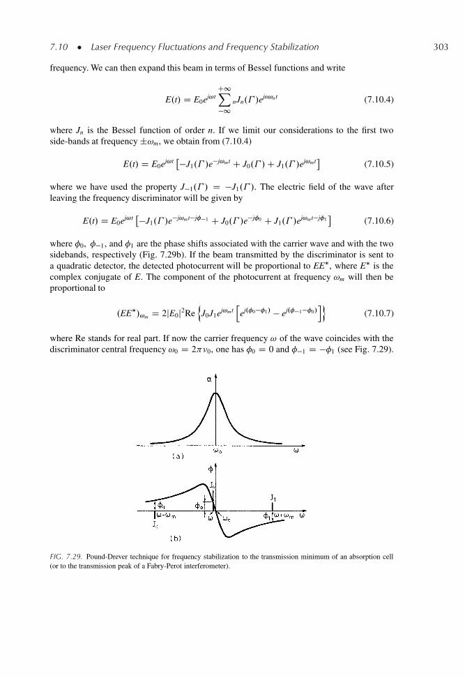
7.10 � Laser Frequency Fluctuations and Frequency Stabilization 303
frequency. We can then expand this beam in terms of Bessel functions and write
E.t/ D E0ej!tC1X�1
nJn.� /ejn!nt (7.10.4)
where Jn is the Bessel function of order n. If we limit our considerations to the first twoside-bands at frequency ˙!m, we obtain from (7.10.4)
E.t/ D E0ej!t��J1.� /e
�j!mt C J0.� /C J1.� /ej!mt
(7.10.5)
where we have used the property J�1.� / D �J1.� /. The electric field of the wave afterleaving the frequency discriminator will be given by
E.t/ D E0ej!t��J1.� /e
�j!mt�j�1 C J0.� /e�j0 C J1.� /e
j!mt�j1
(7.10.6)
where �0, ��1, and �1 are the phase shifts associated with the carrier wave and with the twosidebands, respectively (Fig. 7.29b). If the beam transmitted by the discriminator is sent toa quadratic detector, the detected photocurrent will be proportional to EE�, where E� is thecomplex conjugate of E. The component of the photocurrent at frequency !m will then beproportional to
.EE�/!m D 2jE0j2RenJ0J1ej!mt
hej.0�1/ � ej.�1�0/
io(7.10.7)
where Re stands for real part. If now the carrier frequency ! of the wave coincides with thediscriminator central frequency !0 D 2 �0, one has �0 D 0 and ��1 D ��1 (see Fig. 7.29).
FIG. 7.29. Pound-Drever technique for frequency stabilization to the transmission minimum of an absorption cell(or to the transmission peak of a Fabry-Perot interferometer).
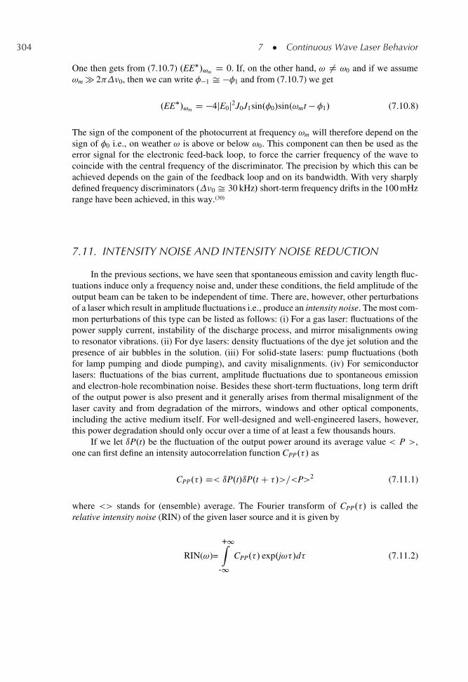
304 7 � Continuous Wave Laser Behavior
One then gets from (7.10.7) .EE�/!m D 0. If, on the other hand, ! ¤ !0 and if we assume!m � 2 �0, then we can write ��1 Š ��1 and from (7.10.7) we get
.EE�/!m D �4jE0j2J0J1sin.�0/sin.!mt � �1/ (7.10.8)
The sign of the component of the photocurrent at frequency !m will therefore depend on thesign of �0 i.e., on weather ! is above or below !0. This component can then be used as theerror signal for the electronic feed-back loop, to force the carrier frequency of the wave tocoincide with the central frequency of the discriminator. The precision by which this can beachieved depends on the gain of the feedback loop and on its bandwidth. With very sharplydefined frequency discriminators .�0 Š 30 kHz/ short-term frequency drifts in the 100 mHzrange have been achieved, in this way..30/
7.11. INTENSITY NOISE AND INTENSITY NOISE REDUCTION
In the previous sections, we have seen that spontaneous emission and cavity length fluc-tuations induce only a frequency noise and, under these conditions, the field amplitude of theoutput beam can be taken to be independent of time. There are, however, other perturbationsof a laser which result in amplitude fluctuations i.e., produce an intensity noise. The most com-mon perturbations of this type can be listed as follows: (i) For a gas laser: fluctuations of thepower supply current, instability of the discharge process, and mirror misalignments owingto resonator vibrations. (ii) For dye lasers: density fluctuations of the dye jet solution and thepresence of air bubbles in the solution. (iii) For solid-state lasers: pump fluctuations (bothfor lamp pumping and diode pumping), and cavity misalignments. (iv) For semiconductorlasers: fluctuations of the bias current, amplitude fluctuations due to spontaneous emissionand electron-hole recombination noise. Besides these short-term fluctuations, long term driftof the output power is also present and it generally arises from thermal misalignment of thelaser cavity and from degradation of the mirrors, windows and other optical components,including the active medium itself. For well-designed and well-engineered lasers, however,this power degradation should only occur over a time of at least a few thousands hours.
If we let ıP.t/ be the fluctuation of the output power around its average value < P >,one can first define an intensity autocorrelation function CPP.�/ as
CPP.�/ D< ıP.t/ıP.t C �/>=<P>2 (7.11.1)
where <> stands for (ensemble) average. The Fourier transform of CPP.�/ is called therelative intensity noise (RIN) of the given laser source and it is given by
RIN(!)=
+1Z-1
CPP.�/ exp.j!�/d� (7.11.2)
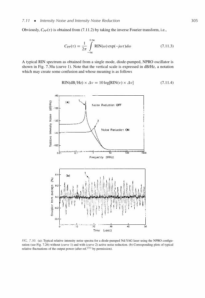
7.11 � Intensity Noise and Intensity Noise Reduction 305
Obviously, CPP.�/ is obtained from (7.11.2) by taking the inverse Fourier transform, i.e.,
CPP.�/ D 1
2
C1Z�1
RIN.!/ exp.�j!�/d! (7.11.3)
A typical RIN spectrum as obtained from a single mode, diode-pumped, NPRO oscillator isshown in Fig. 7.30a (curve 1). Note that the vertical scale is expressed in dB/Hz, a notationwhich may create some confusion and whose meaning is as follows
RIN.dB=Hz/ �� D 10 logŒRIN.�/��� (7.11.4)
FIG. 7.30. (a): Typical relative intensity noise spectra for a diode-pumped Nd:YAG laser using the NPRO configu-ration (see Fig. 7.26) without (curve 1) and with (curve 2) active noise reduction. (b) Corresponding plots of typicalrelative fluctuations of the output power (after ref..31/ by permission).
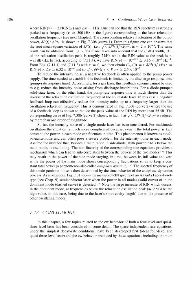
306 7 � Continuous Wave Laser Behavior
where RIN.�/ D 2 RIN.!/ and � D 1 Hz. One can see that the RIN spectrum is stronglypeaked at a frequency (� Š 300 kHz in the figure) corresponding to the laser relaxationoscillation frequency (see next Chapter). The corresponding relative fluctuation of the outputpower, ıP.t/=<P>, is shown in Fig. 7.30b (curve 1). From this figure one can observe thatthe root-mean-square variation of ıP.t/, i.e.,
p< ıP2.t/=<P>2, is � 2 � 10�3. The same
result can be obtained from Fig. 7.30a if one takes into account that the (3 dB) width, �,of the relaxation oscillation peak is roughly 2 kHz while the RIN value at the peak is ��85 dB=Hz. In fact, according to (7.11.4), we have RIN.�/ D 10�8.5 Š 3.16 � 10�9 Hz�1.From Eqs. (7.11.1) and (7.11.3) with � D 0, we then obtain CPP.0/ D< ıP2.t/=<P>2 ŠRIN.�/ �� Š 6.32 � 10�6 and so
p< ıP2.t/= < P >2 Š 2.5 � 10�3.
To reduce the intensity noise, a negative feedback is often applied to the pump powersupply. The time needed to establish this feedback is limited by the discharge response time(pump-rate response time). Accordingly, for a gas laser, this feedback scheme cannot be usedto e.g. reduce the intensity noise arising from discharge instabilities. For a diode-pumpedsolid-state laser, on the other hand, the pump-rate response time is much shorter than theinverse of the relaxation oscillation frequency of the solid state laser. In this case a negativefeedback loop can effectively reduce the intensity noise up to a frequency larger than theoscillation relaxation frequency. This is demonstrated in Fig. 7.30a (curve 2) where the useof a feedback loop is shown to reduce the peak value of the RIN by more than 35 dB. Thecorresponding curve of Fig. 7.30b (curve 2) shows, in fact, that
p< ıP2.t/=<P>2 is reduced
by more than one order of magnitude.So far, the intensity noise of a single mode laser has been considered. For multimode
oscillation the situation is much more complicated because, even if the total power is keptconstant, the power in each mode can fluctuate in time. This phenomenon is known as mode-partition-noise and can often pose a severe problem for the intensity noise in each mode.Assume for instance that, besides a main mode, a side-mode, with power 20 dB below themain mode, is oscillating. The non-linearity of the corresponding rate equations provides amechanism which can lead to anti-correlation between the powers of the two modes..20/ Thismay result in the power of the side mode varying, in time, between its full value and zerowhile the power of the main mode shows corresponding fluctuations so as to keep a con-stant total power (a phenomenon also called antiphase dynamic)..32/ The spectral frequency ofthis mode-partition-noise is then determined by the time behavior of the antiphase-dynamicsprocess. As an example, Fig. 7.31 shows the measured RIN spectra of an AlGaAs Fabry-Perot-type (see Chap. 9) semiconductor laser when the power in all modes (solid curve) or in thedominant mode (dashed curve) is detected..33/ Note the large increase of RIN which occurs,in the dominant mode, at frequencies below the relaxation oscillation peak (Š 2.5 GHz, thehigh value, in this case, being due to the laser’s short cavity length) due to the presence ofother oscillating modes.
7.12. CONCLUSIONS
In this chapter, a few topics related to the cw behavior of both a four-level and quasi-three-level laser has been considered in some detail. The space-independent rate-equations,under the simplest decay-rate conditions, have been developed first (ideal four-level andquasi-three-level laser) and the cw behavior predicted by these equations, including optimum
7.12 � Conclusions 307
FIG. 7.31. Experimental observation of mode partition noise in a multimode semiconductor laser (after ref..33/ bypermission).
coupling conditions, has been considered. The results obtained from the space-dependentequations have then been discussed at some length. It should be recalled that the rate-equationformulation represents the simplest way to describe cw, and transient, laser behavior. Inorder of increasing accuracy, and complexity, one should consider the semiclassical and thequantum electrodynamics treatments. For the cw case, however, the equations for the semi-classical treatment reduce to the rate equations. The full quantum treatment, on the otherhand, is required to correctly describe the start of laser oscillation as well as the fundamen-tal limit to laser frequency noise. When, however, the number of photons in a given cavitymode is much larger than one, the (average) results of the quantum treatment coincide withthose of the semiclassical treatment. It should also be noted that the rate equations, in theirsimplest form as given here, only apply to relatively few cases. In most cases, there are morethan just four levels involved, and the rate equation treatment becomes correspondingly morecomplicated. In fact it could be said that, in general, each laser has its own particular set ofrate equations. The equations considered in this chapter, however, provide a model that canbe readily extended to handle more complicated situations.
Besides topics which can be directly discussed in terms of rate equations, other sub-jects of fundamental importance for cw laser behavior have also been discussed, namely:(i) Reasons for multimode oscillation, methods of single mode selection, and laser tuning.(ii) Limit to monochromaticity, for single mode lasers, as well as field fluctuations of theoutput beam, both in frequency and amplitude. (iii) Methods to actively reduce both fre-quency and amplitude fluctuations. The ensemble of these topics constitute the minimum setof knowledge required for a balanced and up-to-date understanding of cw laser behavior.
308 7 � Continuous Wave Laser Behavior
PROBLEMS
7.1. Calculate the logarithmic loss, � , of a mirror with transmission T D 80% and negligibleinternal loss.
7.2. Prove Eq. (7.2.11)
7.3. With reference to Fig. 7.4 and to example 7.2, taking the value n D 1.82 for the refractive index ofNd:YAG, calculate the equivalent resonator length, Le, and the cavity photon decay time.
7.4. Consider a 4-level laser just at threshold and assume the branching ratio of the 2 ! 1 transitioncompared to the overall spontaneous transition rate is ˇ D 0.51 and assume that the overall upper-state lifetime is purely radiative and equal to � D 230�s (the data refer to the 1.064�m transitionof Nd:YAG, see example 2.13). How short must the lifetime of the lower laser level, 1, be to ensurethat, in the steady state, .N1=N2/ < 1%? Now consider the same laser above threshold and, withreference to example 7.2, assume that the laser is oscillating with an output power Pout D 200 W.How short must the lifetime of the lower laser level be to ensure that, under these conditions,.N1=N2/ < 1%?
7.5. With reference to Fig. 7.4 and to example 7.2, suppose that the Nd:YAG rod is replaced bya Nd:YLF rod of the same dimensions .YLF � YLiF4/. Oscillation can then occur at either� D 1.047�m (extraordinary wave or -transition) or at � D 1.053�m (ordinary wave or�-transition). The largest value of the effective stimulated emission cross section is for the -transition, equal to �e Š 1.8 � 10�19 cm2. The upper state lifetime is the same for the twotransitions, i.e., � D 480�s. Assuming that the internal loss of the cavity and the lamp pump-ing efficiency remain the same as for Nd:YAG, calculate the threshold inversion and the thresholdpump power and compare the results with those of Nd:YAG. Assuming that the energy separationbetween the 4F3=2 upper laser level and the ground level remains the same as for Nd:YAG andtaking the same value of the beam area Ab, calculate the slope efficiency.
7.6. In the case of the previous problem, calculate the optimum output mirror transmission andthe corresponding optimum output power when the laser is pumped by a lamp input powerPp D 7 kW.
7.7. For the high power CO2 laser of Figs 7.7 and 7.8, and with reference to the data considered inexample 7.3, calculate the optimum output coupling and the optimum power for an input pumppower Pp D 140 kW. The resulting optimum value of �2 turns out to be substantially smaller thanthat considered in example 7.3., i.e., the unstable resonator of Fig. 7.7 is substantially overcoupled.This overcoupling is intentional, to increase the peak intensity of the output beam when focusedby a lens. With reference to the focusing properties of the annular beam of an unstable resonatordiscussed in Sect. 5.6.3., show in fact that the � 12 kW beam of Fig. 7.8 (at Pp D 140 kW) producea higher intensity at the focus of a lens compared to that of the optimum beam considered in thisproblem.
7.8. Consider the lamp-pumped Nd:YAG laser of Fig. 7.4. The pumping beam induces a thermal lensof focal length f in the rod whose dioptric power 1=f is proportional to the pump power, Pp. Ata pump power of Pp D 7 kW and for the rod dimensions of Fig. 7.4, the thermal induced focallength is f Š 25 cm..34/ Now assume that, to calculate the cavity mode, the rod of Fig. 7.4 can besimulated by a this lens, of focal length f Š 25 cm, placed at the resonator center. In this case,calculate the TEM00 mode spot size at the lens and at the mirror location.
7.9. One can show that the radial extension of a TEMlm mode of higher order (i.e., for l Š m � 1) isapproximately given by wlm Š p
l w, where w is the spot size of the corresponding TEM00 mode.
Problems 309
The maximum number of Hermite-Gaussian modes that can fit within a rod of radius a will be suchthat wlm Š a..35/ Using this argument and the results obtained in the previous problem, calculatethe approximate number of transverse modes which oscillate in the configuration of Fig. 7.4. Thebeam divergence of a TEMlm mode .l Š m � 1/, lm, is then approximately given by lm Šp
l�= w0, where w0 is the spot size of the TEM00 mode at the beam waist..35/ Calculate then thebeam divergence for the case of Fig. 7.4 assuming that it is equal to the divergence of the highestorder mode which is oscillating.
7.10. Consider the Nd:YAG laser of example 7.4 and assume that the optimum output coupling canbe calculated by the formula established via the space-dependent case of Sect. 7.5. Calculate theoptimum output coupling and, using this value of �2, calculate, with the help of Eq. (7.3.34), theexpected value of the output power at a diode-laser pump power of Pp D 1.14 W.
7.11. Consider a 4 mm diameter 56 mm long 0.9 at. % Nd:YAG rod side-pumped at 807 nm wavelengthby fiber-coupled diode lasers..36/ Assume that the laser is oscillating on a TEM00 mode with aconstant spot-size within the active medium of wa Š 1.4 mm. Let the transmission of the outputmirror be T2 D 15% and assume a total internal loss of �i D 3.8% (see example 7.2). Calculate theoutput power at a laser-diode optical pump power of Pp D 370 W, corresponding to an absorbedpower of Pap D 340 W, and the corresponding slope efficiency. Compare the calculated valueswith the experimental values of ref..36/ and try to explain the discrepancy.
7.12. Consider again the diode-pumped laser of the previous problem, assume that, at the stated pumppower, the thermally-induced lens in the rod has focal length f D 21 cm, and take a symmetricflat-flat resonator as in Fig. 7.4. Under the simplifying assumption that the rod can be simulated bya thin lens of focal length f , calculate the distance of the two plane mirrors from this lens to obtaina spot-size, at the lens position, of wa D 1.4 mm. Calculate also the corresponding spot-size at thetwo mirrors.
7.13. Prove Eq. (7.4.7)
7.14. Consider a He-Ne laser oscillating on its red, � D 632.8 nm in air, transition and assume a lengthof the gas tube of l D 20 cm, a tube radius of 1 mm, a 0.1 Torr partial pressure of Ne atoms, anoutput coupler transmission of 1% and a single pass internal loss of 0.5%. According to exam-ple 2.12, the effective cross section and the overall lifetime of the laser transition can be taken tobe �e D 3 � 10�13 cm2 and � D 150 ns, respectively. Assume, for simplicity, that the lifetime ofthe lower state is much shorter than that of the upper state. Calculate the threshold inversion, theratio of this inversion to the total Ne population, and the critical pump rate. The upper laser level ispredominantly pumped through the 21S state of He which lies � 20.5 eV above the ground state.Assuming unit quantum efficiency in this near-resonant energy-transfer process, calculate the min-imum threshold pump power. For an output power of 3 mW, calculate also the ratio of the numberof photons emitted by stimulated emission to the number of atoms that decay spontaneously.
7.15. An Ar ion laser oscillating on its green, � D 514.5 nm, transition has a 10% unsaturated gain perpass. The resonator consists of two concave spherical mirrors both of radius of curvature R D 5 mand spaced by L D 100 cm. The output mirror has a T2 D 5% transmission while the other mirroris nominally 100% reflecting. Identical apertures are inserted at both ends of the resonator toobtain TEM00 mode operation. Neglecting all other types of losses, calculate the required aperturediameter.
7.16. The linewidth, ��0 D 50 MHz, of a low-pressure CO2 laser is predominantly established by
Doppler broadening. The laser is operating with a pump power twice the threshold value. Assum-ing that one mode coincides with the transition peak and equal losses for all modes, calculate themaximum mirror spacing that would still allow single longitudinal mode operation.
310 7 � Continuous Wave Laser Behavior
7.17. Consider an Ar ion laser oscillating on its green, � D 514.5 nm, transition and assume this transi-tion to be Doppler broadened to a width ��
0 D 3.5 GHz. Assume a cavity length Le D 120 cm,a length of the Ar tube of 100 cm, and take a single pass cavity loss of � D 10%. According toexample 2.12., we can take an effective value of the stimulated emission cross section and upperstate lifetime of �e D 2.5 � 10�13 cm2 and � D 5 ns, respectively. Assume the lifetime of thelower laser level much shorter than that of the upper laser level and that one cavity mode coincideswith the transition peak. Calculate the threshold inversion for this central mode and the thresholdpump rate. At how great a pump rate above threshold does oscillation start on the two adjacentlongitudinal modes?
7.18. A He-Ne laser is oscillating on three adjacent longitudinal modes, the central one being coincidentwith the center of the laser transition. The cavity length is 50 cm and the output coupling 2%.Knowing that the laser linewidth is ��
0 D 1.7 GHz, calculate the mode spacing.
7.19. Assume that one cavity mirror is mounted on a piezoelectric transducer. Show that the combof longitudinal modes shifts by approximately one comb spacing for a �=2 translation of thetransducer.
7.20. Consider a single longitudinal mode He-Ne laser and assume that the oscillating frequency ismade to coincide with the frequency of the transition peak by the use of a piezoelectric transducerattached to a cavity mirror. How far can the mirror be translated before a mode-hop (i.e., a switchof oscillation to the next mode) occurs?
7.21. An Ar ion laser oscillating on its green, � D 514.5 nm, transition has a total loss per pass of 4%,an unsaturated peak gain, Gp D exp.�pNl/, of 1.3, and a cavity length of 100 cm. To select a singlelongitudinal mode, a tilted and coated quartz .nr D 1.45/ Fabry-Perot etalon with a 2 cm thicknessis used inside the resonator. Assuming, for simplicity, that one cavity mode is coincident with thepeak of the transition (whose linewidth is ��
0 D 3.5 GHz), calculate the etalon finesse and thereflectivity of the two etalon faces to ensure single longitudinal mode operation.
7.22. With reference to Fig. 7.31, evaluate the relative root-mean-square fluctuation of the output powerof the semiconductor laser for the dominant mode and for all modes.
References
1. H. Statz and G. de Mars, Transients and Oscillation Pulses in Masers, in Quantum Electronics, ed. byC.H. Townes (Columbia University Press, New York, 1960), pp. 530–537
2. R. Dunsmuir, Theory of Relaxation Oscillations in Optical Masers, J. Electron. Control 10, 453–458 (1961)3. M. Sargent, M.O. Scully, and W.E. Lamb, Laser Physics (Addison-Wesley, London, 1974)4. R. H. Pantell and H.E. Puthoff, Fundamentals of Quantum Electronics, (Wiley, New York, 1969), Chap. 6,
Sect. 6.4.25. W. W. Rigrod, Saturation Effects in High-Gain Lasers, J. Appl. Phys. 36, 2487–2490 (1965)6. L. W. Casperson, Laser Power Calculations: Sources of Error, Appl. Opt. 19, 422–431 (1980)7. W. Koechner, Solid-State Laser Engineering, Vol. 1, Springer Series in Optical Sciences, fourth edition
(Springer-Verlag, Berlin, 1996), Chap. 3, adapted from Fig. 3.218. Reference,.7/ Chap. 3, Fig. 3.229. D. Findlay and R. A. Clay, The Measurement of Internal Losses in 4-Level Lasers, Phys. Lett. 20, 277–278 (1966)
10. Private communication, Istituto di Ricerca per le Tecnologie Meccaniche, Vico Canavese, Torino11. M. C. Fowler, Quantitative Analysis of the Dependence of CO2 Laser Performance on Electrical Discharge
Properties, Appl. Phys. Lett. 18, 175 (1971)12. E. Hoag et al., Performance Characteristics of a 10 kW Industrial CO2 Laser System, Appl. Opt. 13, 1959 (1974)
References 311
13. P. F. Moulton, An Investigation of the Co : MgF2 Laser System, IEEE J. Quant. Electr. QE-21,1582–1588 (1985)
14. V. Evtuhov and A. E. Siegman, A Twisted-Mode Technique for Obtaining Axially Uniform Energy Density in aLaser Cavity, Appl. Opt. 4, 142–143 (1965)
15. J. Berger et al., 370 mW, 1.06�m, cw TEM00 Output from a Nd:YAG Laser Rod End-Pumped by a MonolithicDiode Array, Electr. Lett. 23, 669–670 (1987)
16. W. P. Risk, Modeling of Longitudinally Pumped Solid-State-Lasers Exhibiting Reabsorption Losses, J. Opt. Soc.Am. B 5, 1412–1423 (1988)
17. T. Y. Fan and R. L. Byer, Modeling and CW Operation of a Quasi-Three-Level 946 nm Nd:YAG Laser, IEEE J.Quant. Electr. QE-23, 605–612 (1987)
18. P. Lacovara et al., Room-Temperature Diode-Pumped Yb:YAG Laser, Opt. Lett. 16, 1089–1091 (1991)19. A. Yariv, Energy and Power Considerations in Injection and Optically Pumped Lasers, Proc. IEEE 51, 1723–
1731 (1963)20. C. L. Tang, H. Statz, and G. de Mars, Spectral Output and Spiking Behavior of Solid-State Lasers, J. Appl. Phys.
34, 2289–2295 (1963)21. T. J. Kane and R. L. Byer, Monolithic, Unidirectional Single-Mode Nd:YAG Ring Laser, Opt. Lett. 10, 65 (1985)22. A. E. Siegman, Lasers (University Science Books, Hill Valley, California, 1986), Chap. 12, Sect. 12.223. A. Yariv, Optical Electronics (Saunders College Publishing, Forth Worth, 1991), Sect. 10.724. A. L. Schawlow and C. H. Townes, Infrared and Optical Masers, Phys. Rev. 112, 1940–1949 (1958)25. C. H. Henry, Theory of Linewidth of Semiconductor Lasers, IEEE J. Quant. Electr. QE-18, 259 (1982)26. T. Day, E. K. Gustafson, and R. L. Byer, Sub-Hertz Relative Frequency Stabilization of Two Diode Laser Pumped
Nd:YAG Lasers Locked to a Fabry-Perot Interferometer, IEEE J. Quant. Electr. QE-28, 1106 (1992)27. D. K. Owens and R. Weiss, Measurement of the Phase Fluctuation in a He-Ne Zeeman Laser, Rev. Sci. Instrum.
45, 1060 (1974)28. W. Demtroder, Laser Spectroscopy, Second Edition (Springer-Verlag, Berlin, 1996) Chap. 729. R. W. T. Drever, et al., Laser Phase and Frequency Stabilization using an Optical Resonator, Appl. Phys. B 31,
97–105 (1983)30. N. Uekara and K. Ueda, 193-mHz Beat Linewidth of Frequency Stabilized Laser-Diode-Pumped Nd:YAG Ring
Lasers, Opt. Lett. 18, 505 (1993)31. Introduction to Diode-Pumped Solid-State Lasers, LIGHTWAVE Electronics Corp. Techn. Information
N. 1 (1993)32. K. Otsuka, Winner-Takes-All and Antiphase States in Multimode Lasers, Phys. Rev. Lett. 67, 1090–1093 (1991)33. G. P. Agrawal and N. K. Dutta, Long-Wavelength Semiconductor Lasers, (Van Nostrand Reinhold, New York,
1986), Fig. 6.11, by permission.34. Reference.7/ Sect. 7.1.1. and Fig. 7.535. Reference,.22/ Chapt. 17, Sects. 17.5 and 17.636. D. Golla et al., 62-W CW TEM00 Mode Nd:YAG Laser Side-Pumped by Fiber-Coupled Diode-Lasers, Opt. Lett.
21, 210–212 (1996)
8
Transient Laser Behavior
8.1. INTRODUCTION
In this chapter, we will consider a few cases where the pump rate and/or cavity losses aretime dependent. We will also consider situations in which a nonlinear optical element, such asa saturable absorber, is inserted in the laser cavity, where the non-linearity leads to the laserdeparting from stable cw operation. For these various cases we are thus dealing with transientlaser behavior. The transient cases to be considered can be separated into two categories:(i) Cases, such as relaxation oscillations, Q-switching, gain switching and cavity dumping,where, ideally, a single mode laser is involved and which can be described by a rate equationtreatment. (ii) Cases where many modes are involved, e.g. mode-locking, and for which adifferent treatment needs to be considered. This requires a description in terms of either thefields of all oscillating modes (frequency domain description) or in terms of a self-consistentcirculating pulse within the cavity (time domain description).
8.2. RELAXATION OSCILLATIONS
We will first consider the case of a step-function pump rate. Thus we assume that Rp D 0for t < 0 and Rp.t/ D Rp (independent of time) for t > 0. We will also assume the laser to beoscillating in a single mode so that a simple rate-equation treatment can be properly applied.As seen in the previous chapter, the rate equations are nonlinear in the variables N.t/ and �.t/since they involve products of the form �N. Consequently, analytical solutions for this caseor for other cases about to be considered, are generally not possible and one often needs toresort to numerical computation..1,2/
As a representative example, Fig. 8.1 shows one of the first computed plots of N.t/ and�.t/ as carried out for a three level laser such as a ruby laser..2/ In this case the initial conditionfor the population inversion is N.0/ D �Nt, where Nt is the total population, because, at
O. Svelto, Principles of Lasers,c
313DOI: 10.1007/978-1-4419-1302-9 8, � Springer Science+Business Media LLC 2010
314 8 � Transient Laser Behavior
FIG. 8.1. Example of the temporal behavior of the total inversion, VaN.t/, and photon number, �.t/, for a three-levellaser (after reference,.2/ by permission).
time t D 0, the entire population is in the lower laser level, 1 (see Fig. 1.4a). The initialcondition for the total number of cavity photons is then �.0/ D �i, where �i can be takento be some small integer (e.g. �i D 1) which must just needed to allow laser action start. Itshould also be noted that a similar behavior to that of Fig. 8.1 is also expected for a four-levellaser, one of the main differences being that, in this case, the initial condition is N.0/ D 0.Thus, if the time origin of Fig. 8.1 is shifted approximately to the time t D 2 μs, wherethe population inversion become zero in the figure, the curves of Fig. 8.1 can be used toprovide a qualitative description for the case of a four level laser, as well. Several featuresof this figure are now worth pointing out: (i) After a time t D 2 μs, the population inversionkeeps growing due to the pumping process while the photon number remains at its initial lowvalue, as determined by quantum field fluctuations, until the inversion crosses the thresholdvalue (N0Va D 6.66 � 1015 in the figure). From this time on, roughly for t > 4 μs, thepopulation exceeds the threshold value and the number of cavity photons can begin to grow.From either Eq. (7.2.16b) (four level laser) or Eq. (7.2.24b) (quasi-three level laser) one findsin fact that d�=dt > 0 when N > Nc, where Nc is the critical or threshold inversion. (ii)After threshold is exceeded, the photon number requires some time to grow, from its initialvalue �i D 1, to a value e.g. equal to the steady state value (�0 D 5.8 � 1014 in the figure)and, meanwhile, the population can continue growing due to the pumping process. (iii) Whenthe photon number becomes large enough (roughly when � > �0), the stimulated emissionprocess becomes dominant over the pumping process. The population then begins to decreaseand, at the time corresponding to the maximum of �.t/, N.t/ has dropped back to Nc. Thiscan be readily shown from either Eq. (7.2.16b) or Eq. (7.2.24b) since, when d�=dt D 0, onehas N D Nc. (iv) After this photon peak, the population inversion is then driven below Nc
by the continuing high rate of stimulated emission. Thus the laser goes below threshold andthe photon number also decreases. (v) When this photon number decreases to a sufficientlylow value (roughly when � < �0) the pumping process again becomes dominant over thestimulated emission process. The population inversion can now begin growing again and thewhole series of events considered at points (i)–(iv) repeats itself. The photon number, �.t/, is
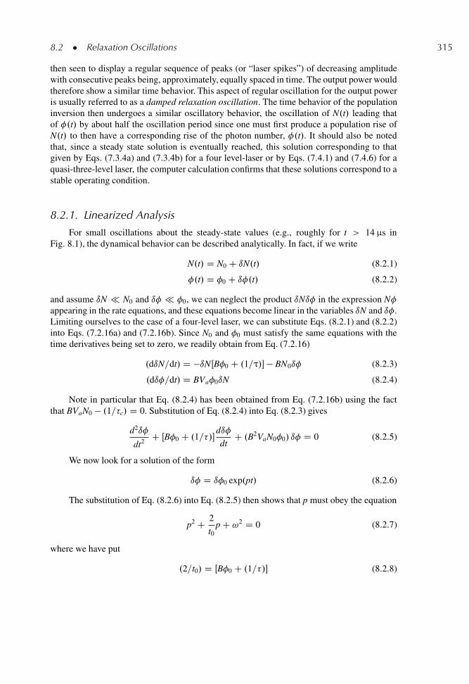
8.2 � Relaxation Oscillations 315
then seen to display a regular sequence of peaks (or “laser spikes”) of decreasing amplitudewith consecutive peaks being, approximately, equally spaced in time. The output power wouldtherefore show a similar time behavior. This aspect of regular oscillation for the output poweris usually referred to as a damped relaxation oscillation. The time behavior of the populationinversion then undergoes a similar oscillatory behavior, the oscillation of N.t/ leading thatof �.t/ by about half the oscillation period since one must first produce a population rise ofN.t/ to then have a corresponding rise of the photon number, �.t/. It should also be notedthat, since a steady state solution is eventually reached, this solution corresponding to thatgiven by Eqs. (7.3.4a) and (7.3.4b) for a four level-laser or by Eqs. (7.4.1) and (7.4.6) for aquasi-three-level laser, the computer calculation confirms that these solutions correspond to astable operating condition.
8.2.1. Linearized Analysis
For small oscillations about the steady-state values (e.g., roughly for t > 14 μs inFig. 8.1), the dynamical behavior can be described analytically. In fact, if we write
N.t/ D N0 C ıN.t/ (8.2.1)
�.t/ D �0 C ı�.t/ (8.2.2)
and assume ıN � N0 and ı� � �0, we can neglect the product ıNı� in the expression N�appearing in the rate equations, and these equations become linear in the variables ıN and ı�.Limiting ourselves to the case of a four-level laser, we can substitute Eqs. (8.2.1) and (8.2.2)into Eqs. (7.2.16a) and (7.2.16b). Since N0 and �0 must satisfy the same equations with thetime derivatives being set to zero, we readily obtain from Eq. (7.2.16)
.dıN=dt/ D �ıNŒB�0 C .1=τ/�� BN0ı� (8.2.3)
.dı�=dt/ D BVa�0ıN (8.2.4)
Note in particular that Eq. (8.2.4) has been obtained from Eq. (7.2.16b) using the factthat BVaN0 � .1=�c/ D 0. Substitution of Eq. (8.2.4) into Eq. (8.2.3) gives
d2ı�
dt2C ŒB�0 C .1=�/�
dı�
dtC .B2VaN0�0/ ı� D 0 (8.2.5)
We now look for a solution of the form
ı� D ı�0 exp.pt/ (8.2.6)
The substitution of Eq. (8.2.6) into Eq. (8.2.5) then shows that p must obey the equation
p2 C 2
t0p C !2 D 0 (8.2.7)
where we have put
.2=t0/ D ŒB�0 C .1=�/� (8.2.8)
316 8 � Transient Laser Behavior
and
!2 D B2VaN0�0 (8.2.9)
The solution of Eq. (8.2.7) is obviously given by
p D � 1
t0˙�
1
t20
� !2
� 1=2
(8.2.10)
The first case we consider is where .1=t0/ < !. In this case the square root in Eq. (8.2.10)gives an imaginary number so that we can write p D �.1=t0/˙ j!0 where
!0 D �!2 � .1=t0/
2 1=2
(8.2.11)
In this case, from Eq. (8.2.6) ı� is seen to correspond to a damped sinusoidaloscillation, i.e.,
ı� D C exp.�t=t0/ sin.!0t C ˇ/ (8.2.12)
where C and ˇ are established by the initial conditions. If Eq. (8.2.12) is then substituted intoEq. (8.2.4) we find that ıN is also described by a damped sinusoidal oscillation. Assuming.1=t0/ � !0, we get
ıN Š !0CBVa�0
exp.�t=t0/ cos.!0t C ˇ/ (8.2.13)
Note that ıN.t/ leads ı�.t/ by half an oscillation period as already discussed previouslysince one must first have a growth of inversion ıN.t/ before one can have a growth of ı�.t/.
Equations (8.2.8) and (8.2.9) can be recast in a form more amenable to calculation if theexplicit expressions for N0 and �0 given by Eqs. (7.3.4a) and (7.3.4b) are used. We readilyobtain
t0 D 2�=x (8.2.14)
! D Œ.x � 1/=�c� �1=2 (8.2.15)
where x D Rp=Rcp, is the amount by which threshold is exceeded. Note that, while the damp-ing time t0 of the oscillation is determined by the upper state lifetime, the oscillation periodT D 2π=!0 Š 2π=! is determined by the geometrical mean of � and the photon lifetime �c.
Example 8.1. Damped oscillation in a Nd:YAG and a GaAs laser We first consider the single modeNd:YAG laser of Fig. 7.26 and assume that the above space-independent relaxation oscillation theory canbe applied to this diode-pumped NPRO laser. Assuming the laser to be x D 5 times above threshold, weobtain from Eq. (8.2.14) t0 D 92 μs, where we have taken � D 230 μs. We will also take l D 11.5 mmas the round trip path length of the NPRO resonator, assume a T D 0.4% output coupling transmission ofthe laser and a round trip cavity loss of L D 0.5%. The round trip loss will then be � Š .T C L/ D 0.9%and the cavity photon decay time �c D nl=c� Š 7.8 ns, where n D 1.82 is the refractive index of the YAG
8.2 � Relaxation Oscillations 317
material. From Eq. (8.2.15) we then obtain � D !=2 Š 238 kHz for the frequency of the relaxationoscillation. Note that, in this case, we have t0 � 1=!, thus the approximation !0 Š ! is justified. Notealso that the spectrum of this damped oscillation is Lorentzian with a width �0 D 1=2 t0 D 1.73 kHz,and this will also be the 3-dB width of the relaxation oscillation peak of the RIN spectrum for this laser(see Fig. 7.30a). Consider next a typical GaAs injection laser with a cavity length L D l D 300 μm, inwhich the two end faces are cleaved and act as the cavity mirrors. According to Eq. (4.3.1) the powerreflectivity of both mirrors will, in this case, be equal to R D Œ.n � 1/=.n C 1/�2 Š 0.3, where n D 3.35is the refractive index of GaAs. We thus have �1 D �2 D � ln R D 1.2. We will also assume a distributedloss coefficient of ˛0 D 60 cm�1 along the semiconductor length, so that we can write �i D ˛0L D 1.8.We thus get � D �i C Œ.�1 C�2/=2� D 3 and �c D Le=c� D nL=c� D 1.1 ps. The upper state lifetime maybe taken to be � Š 3 ns. Assuming x D 1.5 we get from Eq. (8.2.14), t0 D 4 ns, and from Eq. (8.2.15),� D !=2 Š 2 GHz. In this case also we have t0 � 1=! and the approximation!0 Š ! is again justified.Note also that, according to this calculation, the relaxation oscillation peak of the RIN spectrum of thislaser is expected to be in the range of some GHz (see Fig. 7.31).
If the condition t0 > 1=! is not satisfied, the two solutions for p given by Eq. (8.2.10)are both real and negative. In this case the time behavior of ı�.t/ consists of a superpositionof two exponentially damped decays. To have t0 < 1=! we must, according to Eqs. (8.2.14)and (8.2.15), have
.�c=�/ > 4.x � 1/=x2 (8.2.16)
The right hand side of this equation has a maximum value of 1 when x D 2. This meansthat, if �c > � , Eq. (8.2.16) is satisfied for any value of x. This situation usually occurs in gaslasers, which therefore generally do not exhibit spiking behavior.
Example 8.2. Transient behavior of a He-Ne laser Consider a He-Ne laser oscillating on its red transition.� D 632.8 nm/. In this case one has � D 50 ns. Assuming a cavity length of L D 50 cm, an outputcoupling of 1% and neglecting all other losses, we obtain � D �2=2 D 5�10�3, and �c D L=c� D 322 ns.We thus get �c > � and Eq. (8.2.16) is satisfied for any value of x. From Eqs. (8.2.14) and (8.2.15) withx D 1.5, we obtain t0 D 66.6 ns and ! Š 5.6 � 106 Hz. From Eq. (8.2.10) we then see that the twolifetimes describing the decay are 1 μs and 33.3 ns.
Before ending this section it is worth noting that the linearized analysis we have justconsidered also applies to a slightly different case, i.e., when one needs to test the stabilityof a given steady-state solution by a linear stability analysis. We assume, in this case, thatthe laser is already operating in the steady state and that a small step-perturbation is applied(i.e., ıN D ıN0 and ı� D ı�0 at t D 0, where ıN0 and ı�0 are two known quantities).According to the discussion given above the perturbation introduced at time t D 0 will decaywith time either by a damped sinusoidal oscillation or by a biexponential law. The steady statesolutions N0 and �0, which were discussed in the previous Chapter, therefore correspond to astable equilibrium.
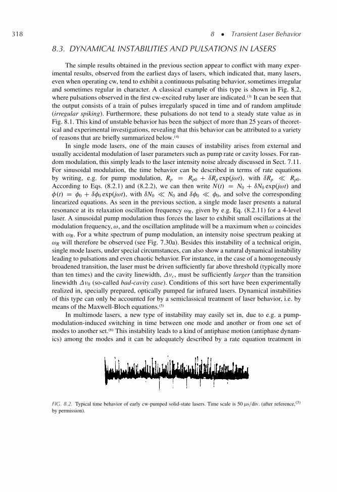
318 8 � Transient Laser Behavior
8.3. DYNAMICAL INSTABILITIES AND PULSATIONS IN LASERS
The simple results obtained in the previous section appear to conflict with many exper-imental results, observed from the earliest days of lasers, which indicated that, many lasers,even when operating cw, tend to exhibit a continuous pulsating behavior, sometimes irregularand sometimes regular in character. A classical example of this type is shown in Fig. 8.2,where pulsations observed in the first cw-excited ruby laser are indicated..3/ It can be seen thatthe output consists of a train of pulses irregularly spaced in time and of random amplitude(irregular spiking). Furthermore, these pulsations do not tend to a steady state value as inFig. 8.1. This kind of unstable behavior has been the subject of more than 25 years of theoret-ical and experimental investigations, revealing that this behavior can be attributed to a varietyof reasons that are briefly summarized below..4/
In single mode lasers, one of the main causes of instability arises from external andusually accidental modulation of laser parameters such as pump rate or cavity losses. For ran-dom modulation, this simply leads to the laser intensity noise already discussed in Sect. 7.11.For sinusoidal modulation, the time behavior can be described in terms of rate equationsby writing, e.g. for pump modulation, Rp D Rp0 C ıRp exp.j!t/, with ıRp � Rp0.According to Eqs. (8.2.1) and (8.2.2), we can then write N.t/ D N0 C ıN0 exp.j!t/ and�.t/ D �0 C ı�0 exp.j!t/, with ıN0 � N0 and ı�0 � �0, and solve the correspondinglinearized equations. As seen in the previous section, a single mode laser presents a naturalresonance at its relaxation oscillation frequency !R, given by e.g. Eq. (8.2.11) for a 4-levellaser. A sinusoidal pump modulation thus forces the laser to exhibit small oscillations at themodulation frequency,!, and the oscillation amplitude will be a maximum when ! coincideswith !R. For a white spectrum of pump modulation, an intensity noise spectrum peaking at!R will therefore be observed (see Fig. 7.30a). Besides this instability of a technical origin,single mode lasers, under special circumstances, can also show a natural dynamical instabilityleading to pulsations and even chaotic behavior. For instance, in the case of a homogeneouslybroadened transition, the laser must be driven sufficiently far above threshold (typically morethan ten times) and the cavity linewidth, �c, must be sufficiently larger than the transitionlinewidth �0 (so-called bad-cavity case). Conditions of this sort have been experimentallyrealized in, specially prepared, optically pumped far infrared lasers. Dynamical instabilitiesof this type can only be accounted for by a semiclassical treatment of laser behavior, i.e. bymeans of the Maxwell-Bloch equations..5/
In multimode lasers, a new type of instability may easily set in, due to e.g. a pump-modulation-induced switching in time between one mode and another or from one set ofmodes to another set..6/ This instability leads to a kind of antiphase motion (antiphase dynam-ics) among the modes and it can be adequately described by a rate equation treatment in
FIG. 8.2. Typical time behavior of early cw-pumped solid-state lasers. Time scale is 50 μs=div. (after reference,.3/
by permission).
8.4 � Q-Switching 319
which, for a homogeneous line, the cross saturation effect due to spatial hole burning is takeninto account..7/
To summarize, we can say that single mode lasers do not usually exhibit dynamical insta-bility but instead show some, possibly quite pronounced, intensity noise due to unavoidableperturbations of laser parameters. On the other hand, multimode lasers may also present addi-tional instabilities due to a kind of antiphase motion among the oscillating modes. Dependingon the amplitude of modulation of the laser parameters, the type of laser, and whether the lineis homogeneously or inhomogeneously broadened, this instability may lead either to a modepartition noise (see Sect. 7.11) or, even, to strong laser pulsations.
8.4. Q-SWITCHING
We have seen in the previous chapter that, under cw operation, the population inversiongets clamped to its threshold value when oscillation starts. Even under the pulsed operatingconditions considered in Sect. 8.2, the population inversion can only exceed the thresholdvalue by a relatively small amount (see Fig. 8.1) due to the onset of stimulated emission.Suppose now that a shutter is introduced into the laser cavity. If the shutter is closed, laseraction is prevented and the population inversion can then reach a value far in excess of thethreshold population for the case where the shutter is absent. If the shutter is now openedsuddenly, the laser will exhibit a gain that greatly exceeds losses and the stored energy willbe released in the form of a short and intense light pulse..8/ Since this operation involvesswitching the cavity Q factor from a low to a high value, the technique is usually calledQ-switching. The technique allows the generation of laser pulses of duration comparable tothe photon decay time (i.e. from a few nanoseconds to a few tens of nanoseconds) and highpeak power (in the megawatt range).
8.4.1. Dynamics of the Q-Switching Process
To describe the Q-switching dynamical behavior, we assume that a step pump pulse isapplied to the laser starting at time t D 0, i.e., Rp.t/ D 0 for t < 0 and Rp.t/ D Rp D const.for 0 < t < tP and that, meanwhile, the shutter is closed (Fig. 8.3a). For 0 < t < tP, the timebehavior of the population inversion can then be calculated from Eq. (7.2.16a), for a 4-levellaser, or Eq. (7.2.24a), for a quasi-3-level laser, with � set to zero. For instance, for a 4-levellaser, we obtain
N.t/ D N1Œ1 � exp.�t=�/� (8.4.1)
where the asymptotic value N1 is given by
N1 D Rp� (8.4.2)
as one can readily obtain from Eq. (7.2.16a) by putting dN=dt D 0. The time behavior ofN.t/ is also shown in Fig. 8.3a. From Eq. (8.4.1) and from Fig. 8.3a we see that the dura-tion tP of the pump pulse should ideally be comparable to or shorter than the upper state
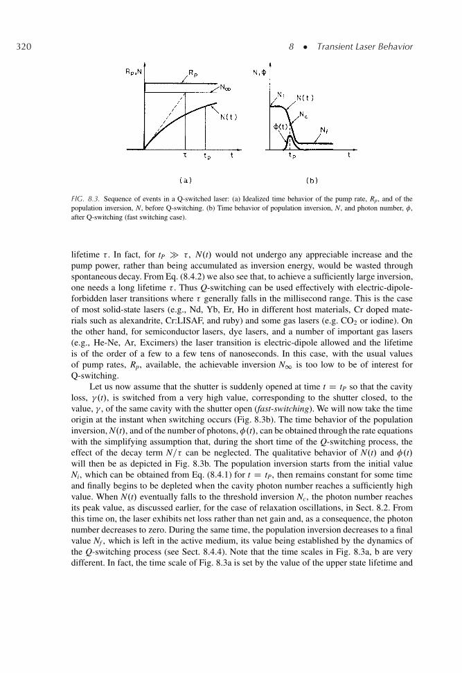
320 8 � Transient Laser Behavior
FIG. 8.3. Sequence of events in a Q-switched laser: (a) Idealized time behavior of the pump rate, Rp, and of thepopulation inversion, N, before Q-switching. (b) Time behavior of population inversion, N, and photon number, �,after Q-switching (fast switching case).
lifetime � . In fact, for tP � � , N.t/ would not undergo any appreciable increase and thepump power, rather than being accumulated as inversion energy, would be wasted throughspontaneous decay. From Eq. (8.4.2) we also see that, to achieve a sufficiently large inversion,one needs a long lifetime � . Thus Q-switching can be used effectively with electric-dipole-forbidden laser transitions where � generally falls in the millisecond range. This is the caseof most solid-state lasers (e.g., Nd, Yb, Er, Ho in different host materials, Cr doped mate-rials such as alexandrite, Cr:LISAF, and ruby) and some gas lasers (e.g. CO2 or iodine). Onthe other hand, for semiconductor lasers, dye lasers, and a number of important gas lasers(e.g., He-Ne, Ar, Excimers) the laser transition is electric-dipole allowed and the lifetimeis of the order of a few to a few tens of nanoseconds. In this case, with the usual valuesof pump rates, Rp, available, the achievable inversion N1 is too low to be of interest forQ-switching.
Let us now assume that the shutter is suddenly opened at time t D tP so that the cavityloss, �.t/, is switched from a very high value, corresponding to the shutter closed, to thevalue, � , of the same cavity with the shutter open (fast-switching). We will now take the timeorigin at the instant when switching occurs (Fig. 8.3b). The time behavior of the populationinversion, N.t/, and of the number of photons, �.t/, can be obtained through the rate equationswith the simplifying assumption that, during the short time of the Q-switching process, theeffect of the decay term N=� can be neglected. The qualitative behavior of N.t/ and �.t/will then be as depicted in Fig. 8.3b. The population inversion starts from the initial valueNi, which can be obtained from Eq. (8.4.1) for t D tP, then remains constant for some timeand finally begins to be depleted when the cavity photon number reaches a sufficiently highvalue. When N.t/ eventually falls to the threshold inversion Nc, the photon number reachesits peak value, as discussed earlier, for the case of relaxation oscillations, in Sect. 8.2. Fromthis time on, the laser exhibits net loss rather than net gain and, as a consequence, the photonnumber decreases to zero. During the same time, the population inversion decreases to a finalvalue Nf , which is left in the active medium, its value being established by the dynamics ofthe Q-switching process (see Sect. 8.4.4). Note that the time scales in Fig. 8.3a, b are verydifferent. In fact, the time scale of Fig. 8.3a is set by the value of the upper state lifetime and
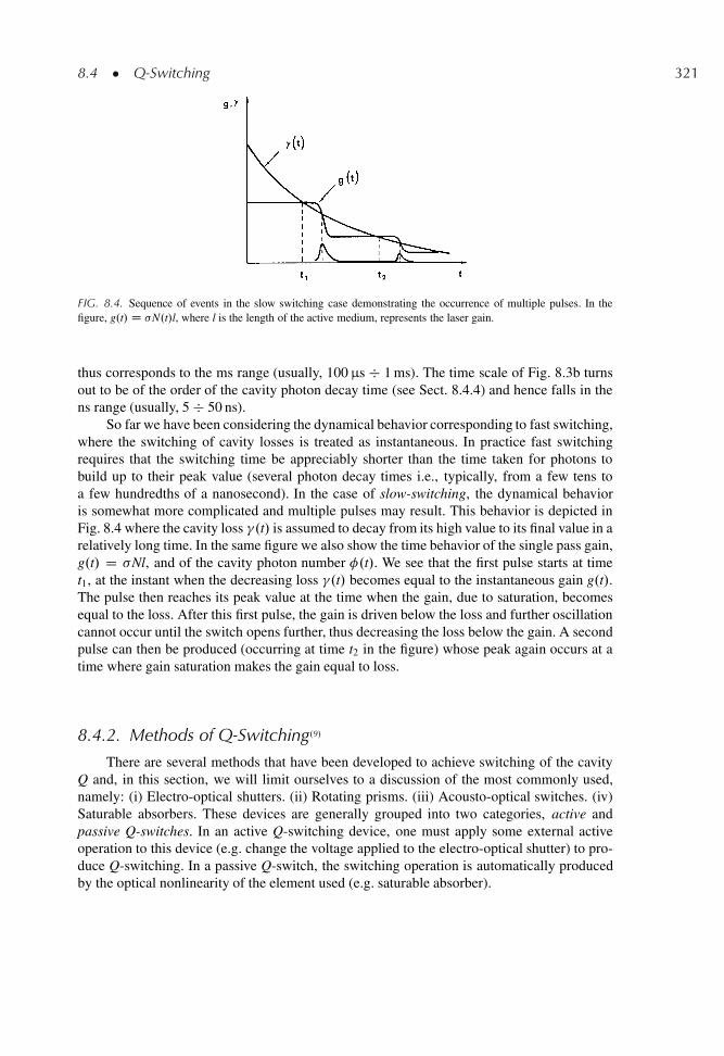
8.4 � Q-Switching 321
FIG. 8.4. Sequence of events in the slow switching case demonstrating the occurrence of multiple pulses. In thefigure, g.t/ D �N.t/l, where l is the length of the active medium, represents the laser gain.
thus corresponds to the ms range (usually, 100 μs � 1 ms). The time scale of Fig. 8.3b turnsout to be of the order of the cavity photon decay time (see Sect. 8.4.4) and hence falls in thens range (usually, 5 � 50 ns).
So far we have been considering the dynamical behavior corresponding to fast switching,where the switching of cavity losses is treated as instantaneous. In practice fast switchingrequires that the switching time be appreciably shorter than the time taken for photons tobuild up to their peak value (several photon decay times i.e., typically, from a few tens toa few hundredths of a nanosecond). In the case of slow-switching, the dynamical behavioris somewhat more complicated and multiple pulses may result. This behavior is depicted inFig. 8.4 where the cavity loss �.t/ is assumed to decay from its high value to its final value in arelatively long time. In the same figure we also show the time behavior of the single pass gain,g.t/ D �Nl, and of the cavity photon number �.t/. We see that the first pulse starts at timet1, at the instant when the decreasing loss �.t/ becomes equal to the instantaneous gain g.t/.The pulse then reaches its peak value at the time when the gain, due to saturation, becomesequal to the loss. After this first pulse, the gain is driven below the loss and further oscillationcannot occur until the switch opens further, thus decreasing the loss below the gain. A secondpulse can then be produced (occurring at time t2 in the figure) whose peak again occurs at atime where gain saturation makes the gain equal to loss.
8.4.2. Methods of Q-Switching.9/
There are several methods that have been developed to achieve switching of the cavityQ and, in this section, we will limit ourselves to a discussion of the most commonly used,namely: (i) Electro-optical shutters. (ii) Rotating prisms. (iii) Acousto-optical switches. (iv)Saturable absorbers. These devices are generally grouped into two categories, active andpassive Q-switches. In an active Q-switching device, one must apply some external activeoperation to this device (e.g. change the voltage applied to the electro-optical shutter) to pro-duce Q-switching. In a passive Q-switch, the switching operation is automatically producedby the optical nonlinearity of the element used (e.g. saturable absorber).
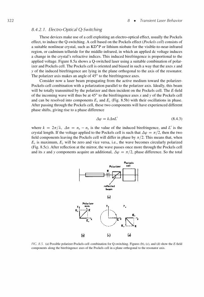
322 8 � Transient Laser Behavior
8.4.2.1. Electro-Optical Q-Switching
These devices make use of a cell exploiting an electro-optical effect, usually the Pockelseffect, to induce the Q-switching. A cell based on the Pockels effect (Pockels cell) consists ofa suitable nonlinear crystal, such as KD�P or lithium niobate for the visible-to-near-infraredregion, or cadmium telluride for the middle-infrared, in which an applied dc voltage inducesa change in the crystal’s refractive indices. This induced birefringence is proportional to theapplied voltage. Figure 8.5a shows a Q-switched laser using a suitable combination of polar-izer and Pockels cell. The Pockels cell is oriented and biased in such a way that the axes x andy of the induced birefringence are lying in the plane orthogonal to the axis of the resonator.The polarizer axis makes an angle of 45ı to the birefringence axes.
Consider now a laser beam propagating from the active medium toward the polarizer-Pockels-cell combination with a polarization parallel to the polarizer axis. Ideally, this beamwill be totally transmitted by the polarizer and then incident on the Pockels cell. The E-fieldof the incoming wave will thus be at 45ı to the birefringence axes x and y of the Pockels celland can be resolved into components Ex and Ey (Fig. 8.5b) with their oscillations in phase.After passing through the Pockels cell, these two components will have experienced differentphase shifts, giving rise to a phase difference
' D knL0 (8.4.3)
where k D 2 =�, n D nx � ny is the value of the induced birefringence, and L0 is thecrystal length. If the voltage applied to the Pockels cell is such that ' D =2, then the twofield components leaving the Pockels cell will differ in phase by =2. This means that, whenEx is maximum, Ey will be zero and vice versa, i.e., the wave becomes circularly polarized(Fig. 8.5c). After reflection at the mirror, the wave passes once more through the Pockels celland its x and y components acquire an additional, ' D =2, phase difference. So the total
FIG. 8.5. (a) Possible polarizer-Pockels-cell combination for Q-switching. Figures (b), (c), and (d) show the E-fieldcomponents along the birefringence axes of the Pockels cell in a plane orthogonal to the resonator axis.
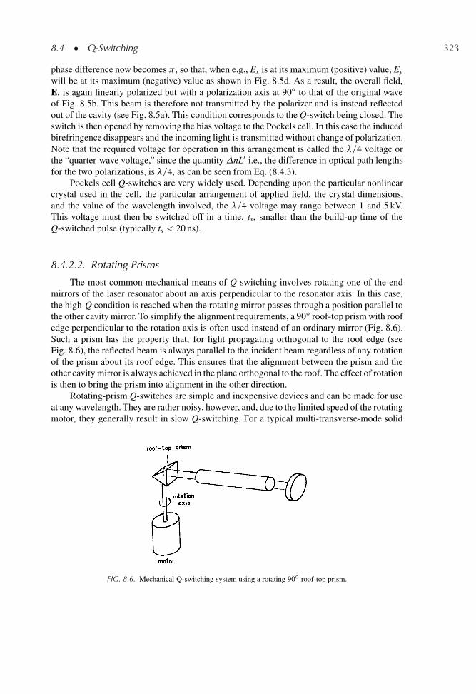
8.4 � Q-Switching 323
phase difference now becomes , so that, when e.g., Ex is at its maximum (positive) value, Ey
will be at its maximum (negative) value as shown in Fig. 8.5d. As a result, the overall field,E, is again linearly polarized but with a polarization axis at 90ı to that of the original waveof Fig. 8.5b. This beam is therefore not transmitted by the polarizer and is instead reflectedout of the cavity (see Fig. 8.5a). This condition corresponds to the Q-switch being closed. Theswitch is then opened by removing the bias voltage to the Pockels cell. In this case the inducedbirefringence disappears and the incoming light is transmitted without change of polarization.Note that the required voltage for operation in this arrangement is called the �=4 voltage orthe “quarter-wave voltage,” since the quantity nL0 i.e., the difference in optical path lengthsfor the two polarizations, is �=4, as can be seen from Eq. (8.4.3).
Pockels cell Q-switches are very widely used. Depending upon the particular nonlinearcrystal used in the cell, the particular arrangement of applied field, the crystal dimensions,and the value of the wavelength involved, the �=4 voltage may range between 1 and 5 kV.This voltage must then be switched off in a time, ts, smaller than the build-up time of theQ-switched pulse (typically ts < 20 ns).
8.4.2.2. Rotating Prisms
The most common mechanical means of Q-switching involves rotating one of the endmirrors of the laser resonator about an axis perpendicular to the resonator axis. In this case,the high-Q condition is reached when the rotating mirror passes through a position parallel tothe other cavity mirror. To simplify the alignment requirements, a 90ı roof-top prism with roofedge perpendicular to the rotation axis is often used instead of an ordinary mirror (Fig. 8.6).Such a prism has the property that, for light propagating orthogonal to the roof edge (seeFig. 8.6), the reflected beam is always parallel to the incident beam regardless of any rotationof the prism about its roof edge. This ensures that the alignment between the prism and theother cavity mirror is always achieved in the plane orthogonal to the roof. The effect of rotationis then to bring the prism into alignment in the other direction.
Rotating-prism Q-switches are simple and inexpensive devices and can be made for useat any wavelength. They are rather noisy, however, and, due to the limited speed of the rotatingmotor, they generally result in slow Q-switching. For a typical multi-transverse-mode solid
FIG. 8.6. Mechanical Q-switching system using a rotating 90ı roof-top prism.
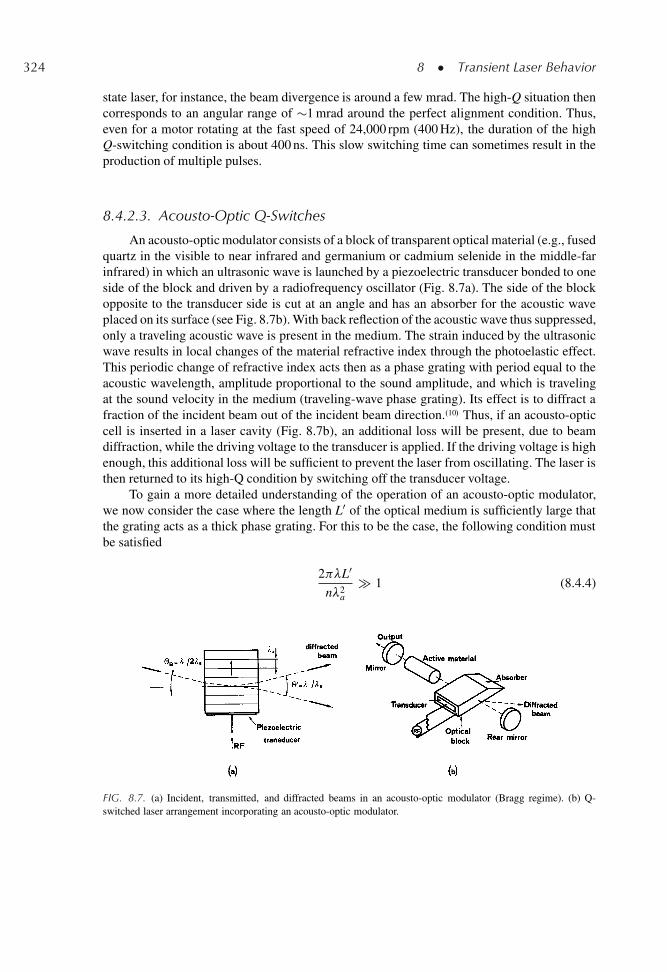
324 8 � Transient Laser Behavior
state laser, for instance, the beam divergence is around a few mrad. The high-Q situation thencorresponds to an angular range of �1 mrad around the perfect alignment condition. Thus,even for a motor rotating at the fast speed of 24,000 rpm (400 Hz), the duration of the highQ-switching condition is about 400 ns. This slow switching time can sometimes result in theproduction of multiple pulses.
8.4.2.3. Acousto-Optic Q-Switches
An acousto-optic modulator consists of a block of transparent optical material (e.g., fusedquartz in the visible to near infrared and germanium or cadmium selenide in the middle-farinfrared) in which an ultrasonic wave is launched by a piezoelectric transducer bonded to oneside of the block and driven by a radiofrequency oscillator (Fig. 8.7a). The side of the blockopposite to the transducer side is cut at an angle and has an absorber for the acoustic waveplaced on its surface (see Fig. 8.7b). With back reflection of the acoustic wave thus suppressed,only a traveling acoustic wave is present in the medium. The strain induced by the ultrasonicwave results in local changes of the material refractive index through the photoelastic effect.This periodic change of refractive index acts then as a phase grating with period equal to theacoustic wavelength, amplitude proportional to the sound amplitude, and which is travelingat the sound velocity in the medium (traveling-wave phase grating). Its effect is to diffract afraction of the incident beam out of the incident beam direction..10/ Thus, if an acousto-opticcell is inserted in a laser cavity (Fig. 8.7b), an additional loss will be present, due to beamdiffraction, while the driving voltage to the transducer is applied. If the driving voltage is highenough, this additional loss will be sufficient to prevent the laser from oscillating. The laser isthen returned to its high-Q condition by switching off the transducer voltage.
To gain a more detailed understanding of the operation of an acousto-optic modulator,we now consider the case where the length L0 of the optical medium is sufficiently large thatthe grating acts as a thick phase grating. For this to be the case, the following condition mustbe satisfied
2 �L0
n�2a
� 1 (8.4.4)
FIG. 8.7. (a) Incident, transmitted, and diffracted beams in an acousto-optic modulator (Bragg regime). (b) Q-switched laser arrangement incorporating an acousto-optic modulator.
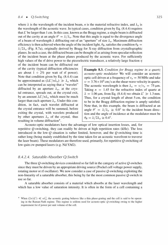
8.4 � Q-Switching 325
where � is the wavelength of the incident beam, n is the material refractive index, and �a isthe wavelength of the acoustic wave. In typical cases, condition given by Eq. (8.4.4) requiresthat L0 be larger than 1 cm. In this case, known as the Bragg regime, a single beam is diffractedout of the cavity at an angle 0 D �=�a. Note that this angle is equal to the divergence angleof a beam of wavelength � diffracting out of an “aperture” of size �a. Maximum diffractionefficiency is then achieved when the angle of the incident light, B, satisfies the condition B D�=2�a (Fig. 8.7a), originally derived by Bragg for X-ray diffraction from crystallographicplanes. In such a case, the diffracted beam can be thought of as arising from specular reflectionof the incident beam at the phase planes produced by the acoustic wave. For sufficientlyhigh values of the rf drive power to the piezoelectric transducer, a relatively large fraction �
Example 8.3. Condition for Bragg regime in a quartzacousto-optic modulator We will consider an acousto-optic cell driven at a frequency of �a D 50 MHz and take� D 3.76�105 cm=s as the shear-wave velocity in quartz.The acoustic wavelength is then �a D �=�a D 75 μm.Taking n D 1.45 for the refractive index of quartz at� D 1.06 μm, from Eq. (8.4.4) we obtain L0 � 1.3 mm.Thus, for a crystal length of about 5 cm, the conditionto be in the Bragg diffraction regime is amply satisfied.Note that, in this example, the beam is diffracted at anangle 0 D �=�a Š 0.8ı to the incident beam direc-tion and the angle of incidence at the modulator must beB D �=2�a Š 0.4ı.
of the incident beam can be diffracted outof the cavity (typical diffraction efficienciesare about 1 � 2% per watt of rf power).Note that condition given by Eq. (8.4.4) canbe approximated as .�L0=n�a/ � �a whichcan be interpreted as saying that a “wavelet”diffracted by an aperture �a, at the crys-tal entrance, spreads out, at the crystal exit,by an amount �L0=n�a which must be muchlarger than each aperture �a. Under this con-dition, in fact, each wavelet diffracted atthe crystal entrance will be summed, beforeexiting the crystal, with wavelets producedby other apertures �a of the crystal, thusresulting in volume diffraction�.
Acousto-optic modulators have the advantage of low optical insertion losses, and, forrepetitive Q-switching, they can readily be driven at high repetition rates (kHz). The lossintroduced in the low-Q situation is rather limited, however, and the Q-switching time israther long (being mainly established by the time taken for an acoustic wavefront to traversethe laser beam). These modulators are therefore used, primarily, for repetitive Q-switching oflow-gain cw-pumped lasers (e.g. Nd:YAG).
8.4.2.4. Saturable-Absorber Q-Switch
The three Q-switching devices considered so far fall in the category of active Q-switchessince they must be driven by an appropriate driving source (Pockel cell voltage power supply,rotating motor or rf oscillator). We now consider a case of passive Q-switching exploiting thenon-linearity of a saturable absorber, this being by far the most common passive Q-switch inuse so far.
A saturable absorber consists of a material which absorbs at the laser wavelength andwhich has a low value of saturation intensity. It is often in the form of a cell containing a
� When .2 �L0/ n�2a, the acoustic grating behaves like a thin phase-grating and the cell is said to be operat-
ing in the Raman-Nath regime. This regime is seldom used for acousto-optic Q-switching owing to the higherrequirement for rf power per unit volume of the cell.
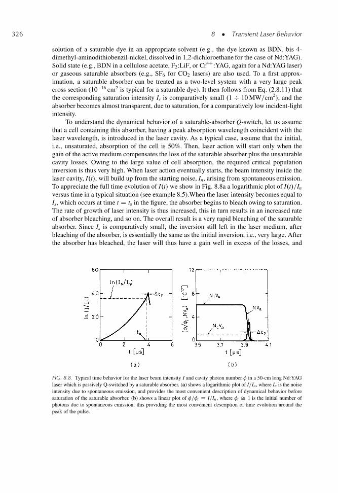
326 8 � Transient Laser Behavior
solution of a saturable dye in an appropriate solvent (e.g., the dye known as BDN, bis 4-dimethyl-aminodithiobenzil-nickel, dissolved in 1,2-dichloroethane for the case of Nd:YAG).Solid state (e.g., BDN in a cellulose acetate, F2:LiF, or Cr4C:YAG, again for a Nd:YAG laser)or gaseous saturable absorbers (e.g., SF6 for CO2 lasers) are also used. To a first approx-imation, a saturable absorber can be treated as a two-level system with a very large peakcross section (10�16 cm2 is typical for a saturable dye). It then follows from Eq. (2.8.11) thatthe corresponding saturation intensity Is is comparatively small .1 � 10 MW=cm2/, and theabsorber becomes almost transparent, due to saturation, for a comparatively low incident-lightintensity.
To understand the dynamical behavior of a saturable-absorber Q-switch, let us assumethat a cell containing this absorber, having a peak absorption wavelength coincident with thelaser wavelength, is introduced in the laser cavity. As a typical case, assume that the initial,i.e., unsaturated, absorption of the cell is 50%. Then, laser action will start only when thegain of the active medium compensates the loss of the saturable absorber plus the unsaturablecavity losses. Owing to the large value of cell absorption, the required critical populationinversion is thus very high. When laser action eventually starts, the beam intensity inside thelaser cavity, I.t/, will build up from the starting noise, In, arising from spontaneous emission.To appreciate the full time evolution of I.t/ we show in Fig. 8.8a a logarithmic plot of I.t/=In
versus time in a typical situation (see example 8.5).When the laser intensity becomes equal toIs, which occurs at time t D ts in the figure, the absorber begins to bleach owing to saturation.The rate of growth of laser intensity is thus increased, this in turn results in an increased rateof absorber bleaching, and so on. The overall result is a very rapid bleaching of the saturableabsorber. Since Is is comparatively small, the inversion still left in the laser medium, afterbleaching of the absorber, is essentially the same as the initial inversion, i.e., very large. Afterthe absorber has bleached, the laser will thus have a gain well in excess of the losses, and
FIG. 8.8. Typical time behavior for the laser beam intensity I and cavity photon number � in a 50-cm long Nd:YAGlaser which is passively Q-switched by a saturable absorber. (a) shows a logarithmic plot of I=In , where In is the noiseintensity due to spontaneous emission, and provides the most convenient description of dynamical behavior beforesaturation of the saturable absorber. (b) shows a linear plot of �=�i D I=In , where �i Š 1 is the initial number ofphotons due to spontaneous emission, this providing the most convenient description of time evolution around thepeak of the pulse.
8.4 � Q-Switching 327
a giant pulse will be produced. The dynamical behavior during this last phase is illustratedin more detail in Fig. 8.8b, where the quantity �.t/=�i D I.t/=In Œ�.t/ is the cavity photonnumber and �i Š 1 is the initial value due to spontaneous emission] is now plotted vs time, ina linear scale and in a restricted time interval. The time behavior of the total inversion NVa,where Va is the volume of the mode in the active medium, is also shown in the same figure (seeexample 8.5). One sees that, as in any other Q-switching case, the photon number now keepsincreasing rapidly until saturation of the inversion and hence of the gain sets in. The pulsethus reaches a maximum value when the inversion becomes equal to the critical inversion, Nc,of the laser without saturable absorber and the pulse thereafter decreases.
An important feature to be noticed from Fig. 8.8 is that the time taken for the pulse toincrease from the noise level to the peak value is very long .tp Š 3.94 μs/. This is essentiallydue to the fact that, during the unbleached phase of the saturable absorber, i.e. for t < ts,laser gain barely exceeds the high threshold value established by the presence of the, as yetunsaturated, absorber. The growth of laser intensity is thus very slow and a large number ofpasses is required for the beam to reach its peak value (�2,370 in the example consideredin Fig. 8.8). This results in a natural selection of cavity modes..11/ Suppose in fact that twomodes have single pass unsaturated gains g1 and g2 .g D �Nl/ and single pass losses �1 and�2. Since the two modes start from the same intensity as established by spontaneous emission,the ratio of the two intensities, at time t D ts, i.e., before saturable absorber saturation, will begiven by
I1
I2D"
e.g1�1/
e.g2�2/
#n
(8.4.5)
where n is the number of round trips within the cavity up to a time t D ts (n Š 2, 310 in theexample of Fig. 8.8). If we now let ı D .g1 ��1/�.g2 ��2/ be the difference between the twonet gains, from Eq. (8.4.5) we can write .I1=I2/ D exp nı. We thus see that, even assuming thevery modest value for ı of 0.001, for n D 2, 310 we get .I1=I2/ D exp 2.3 Š 10. Thus evena very modest discrimination of either gain or loss between the two modes results in a largediscrimination between their intensities at time t D ts, and hence also at the peak of the pulse,which occurs shortly afterward (�100 ns in the example). As a result, single-mode operationcan be achieved rather easily in the case of a saturable absorber Q-switch. Note that, in thecase of active Q-switching, this mode selection mechanism is much less effective since thelaser build-up from noise is much faster and the total number of transits may now be of theorder of only 10 or 20�.
Passive Q-switching by saturable absorbers provides the simplest method ofQ-switching. Photochemical degradation of the absorber, particularly for dye saturableabsorbers, was the main drawback to this type of Q-switch. This situation is now changingwith the advent of solid-state absorbers which do not degrade. The use of passive Q-switchinghas therefore mainly restricted to low average-power devices.
� It should be noted, however, that one can operate an active Q-switch in an analogous fashion to the saturableabsorber by setting the low Q (high loss) condition to a value that permits lasing to start (known as “prelasing”)before gradually switching to high Q after a long prelase has allowed mode selection to occur..38/
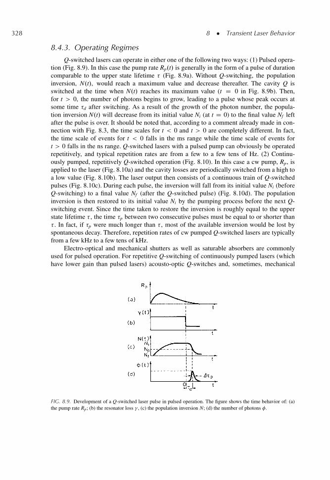
328 8 � Transient Laser Behavior
8.4.3. Operating Regimes
Q-switched lasers can operate in either one of the following two ways: (1) Pulsed opera-tion (Fig. 8.9). In this case the pump rate Rp.t/ is generally in the form of a pulse of durationcomparable to the upper state lifetime � (Fig. 8.9a). Without Q-switching, the populationinversion, N.t/, would reach a maximum value and decrease thereafter. The cavity Q isswitched at the time when N.t/ reaches its maximum value (t D 0 in Fig. 8.9b). Then,for t > 0, the number of photons begins to grow, leading to a pulse whose peak occurs atsome time �d after switching. As a result of the growth of the photon number, the popula-tion inversion N.t/ will decrease from its initial value Ni (at t D 0) to the final value Nf leftafter the pulse is over. It should be noted that, according to a comment already made in con-nection with Fig. 8.3, the time scales for t < 0 and t > 0 are completely different. In fact,the time scale of events for t < 0 falls in the ms range while the time scale of events fort > 0 falls in the ns range. Q-switched lasers with a pulsed pump can obviously be operatedrepetitively, and typical repetition rates are from a few to a few tens of Hz. (2) Continu-ously pumped, repetitively Q-switched operation (Fig. 8.10). In this case a cw pump, Rp, isapplied to the laser (Fig. 8.10a) and the cavity losses are periodically switched from a high toa low value (Fig. 8.10b). The laser output then consists of a continuous train of Q-switchedpulses (Fig. 8.10c). During each pulse, the inversion will fall from its initial value Ni (beforeQ-switching) to a final value Nf (after the Q-switched pulse) (Fig. 8.10d). The populationinversion is then restored to its initial value Ni by the pumping process before the next Q-switching event. Since the time taken to restore the inversion is roughly equal to the upperstate lifetime � , the time �p between two consecutive pulses must be equal to or shorter than� . In fact, if �p were much longer than � , most of the available inversion would be lost byspontaneous decay. Therefore, repetition rates of cw pumped Q-switched lasers are typicallyfrom a few kHz to a few tens of kHz.
Electro-optical and mechanical shutters as well as saturable absorbers are commonlyused for pulsed operation. For repetitive Q-switching of continuously pumped lasers (whichhave lower gain than pulsed lasers) acousto-optic Q-switches and, sometimes, mechanical
FIG. 8.9. Development of a Q-switched laser pulse in pulsed operation. The figure shows the time behavior of: (a)the pump rate Rp; (b) the resonator loss � , (c) the population inversion N; (d) the number of photons �.
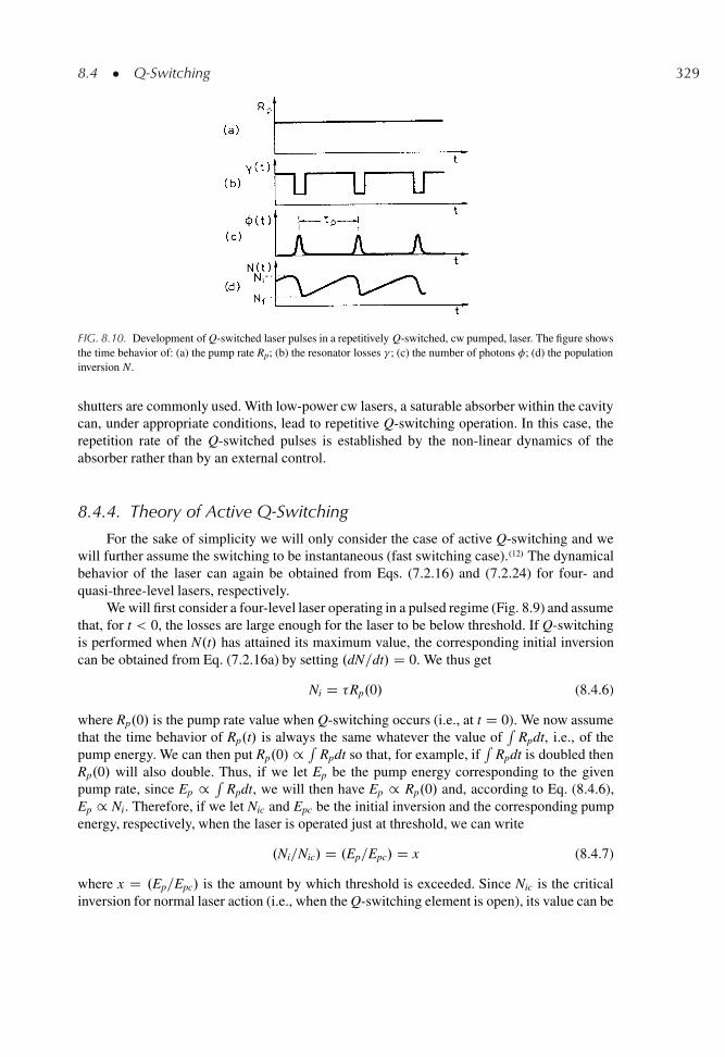
8.4 � Q-Switching 329
FIG. 8.10. Development of Q-switched laser pulses in a repetitively Q-switched, cw pumped, laser. The figure showsthe time behavior of: (a) the pump rate Rp; (b) the resonator losses � ; (c) the number of photons �; (d) the populationinversion N.
shutters are commonly used. With low-power cw lasers, a saturable absorber within the cavitycan, under appropriate conditions, lead to repetitive Q-switching operation. In this case, therepetition rate of the Q-switched pulses is established by the non-linear dynamics of theabsorber rather than by an external control.
8.4.4. Theory of Active Q-Switching
For the sake of simplicity we will only consider the case of active Q-switching and wewill further assume the switching to be instantaneous (fast switching case)..12/ The dynamicalbehavior of the laser can again be obtained from Eqs. (7.2.16) and (7.2.24) for four- andquasi-three-level lasers, respectively.
We will first consider a four-level laser operating in a pulsed regime (Fig. 8.9) and assumethat, for t < 0, the losses are large enough for the laser to be below threshold. If Q-switchingis performed when N.t/ has attained its maximum value, the corresponding initial inversioncan be obtained from Eq. (7.2.16a) by setting .dN=dt/ D 0. We thus get
Ni D �Rp.0/ (8.4.6)
where Rp.0/ is the pump rate value when Q-switching occurs (i.e., at t D 0). We now assumethat the time behavior of Rp.t/ is always the same whatever the value of
RRpdt, i.e., of the
pump energy. We can then put Rp.0/ / RRpdt so that, for example, if
RRpdt is doubled then
Rp.0/ will also double. Thus, if we let Ep be the pump energy corresponding to the givenpump rate, since Ep / R
Rpdt, we will then have Ep / Rp.0/ and, according to Eq. (8.4.6),Ep / Ni. Therefore, if we let Nic and Epc be the initial inversion and the corresponding pumpenergy, respectively, when the laser is operated just at threshold, we can write
.Ni=Nic/ D .Ep=Epc/ D x (8.4.7)
where x D .Ep=Epc/ is the amount by which threshold is exceeded. Since Nic is the criticalinversion for normal laser action (i.e., when the Q-switching element is open), its value can be
330 8 � Transient Laser Behavior
obtained by the usual critical inversion relation i.e., Nic D Nc D �=� l, where � is the cavityloss with the Q-switching element open. If Nic is known, i.e., if � , � , and l are known, andif the ratio x between the actual pump energy and the threshold pump energy is also known,then Eq. (8.4.7) allows the initial inversion, Ni, to be readily calculated.
Once Ni is known, the time evolution of the system after Q-switching, i.e., for t > 0,can be obtained from Eq. (7.2.16) with the initial conditions N.0/ D Ni and �.0/ D �i. Hereagain �i is just some small number of photons needed to let laser action start Œ�i Š 1�. Theequations can now be considerably simplified since we expect the evolution of both N.t/ and�.t/ to occur on a time scale so short that the pump term Rp and the spontaneous decay termN=� in (7.2.16a) can be neglected. Equations (7.2.16) then reduce to
dN
dtD �B�N (8.4.8a)
d�
dtD�
VaBN � 1
�c
�� (8.4.8b)
Before proceeding it is worth remembering that, according to Eq. (8.2.12), the populationNp corresponding to the peak of the photon pulse (see Fig. 8.9c), i.e., when .d�=dt/ D 0, is
Np D 1=VaB�c D �=� l (8.4.9)
which is the same as the critical inversion Nc. This result, with the help of Eq. (8.4.7), allowsus to express the ratio Ni=Np in a form that will be useful for the discussion that follows, viz.,
.Ni=Np/ D x (8.4.10)
After these preliminary considerations, we are ready to proceed with a calculation of the peakpower of the laser output pulse, Pp, through, e.g., mirror 2. According to Eq. (7.2.18) we have
Pp D��2c
2Le
�h��p (8.4.11)
where �p is the number of photons in the cavity at the peak of the laser pulse. To calculate �p
we take the ratio between Eqs. (8.4.8a) and (8.4.8b). Using Eq. (8.4.9) also, we get
d�
dND �Va
�1 � Np
N
�(8.4.12)
which can be readily integrated to give
� D VaŒNi � N � Np ln.Ni=N/� (8.4.13)
where, for simplicity, the small number �i has been neglected. At the peak of the pulse wethen get
�p D VaNp
�Ni
Np� ln
Ni
Np� 1
�(8.4.14)
which readily gives �p once Np and the ratio .Ni=Np/ are known through Eqs. (8.4.9)and (8.4.10) respectively. The peakpower is then obtained from Eqs. (8.4.11), (8.4.14)
8.4 � Q-Switching 331
and (8.4.9) as
Pp D �2
2
�Ab
�
� �h�
�c
� �Ni
Np� ln
Ni
Np� 1
�(8.4.15)
where Ab D Va=l is the beam area and where the expression for �c, given by Eq. (7.2.14), hasalso been used.
To calculate the output energy, E, we begin by noticing that
E D1Z
0
P.t/dt D��2c
2Le
�h�
1Z0
�dt (8.4.16)
where P.t/ is the time behavior of the output power and where Eq. (7.2.18) has been usedagain. The integration in Eq. (8.4.16) can be carried out easily by integrating both sides ofEq. (8.4.8b) and by noting that �.0/ D �.1/ Š 0. We then get
R10 �dt D Va�c
R10 B�Ndt.
The quantityR1
0 B�Ndt can then be obtained by integrating both sides of Eq. (8.4.8a), togive
R10 B�Ndt D .Ni � Nf / where Nf is the final inversion (see Fig. 8.3b). We thus getR1
0 �dt D Va�c.Ni � Nf / so that Eq. (8.4.16) becomes
E D .�2=2�/.Ni � Nf /.Vah�/ (8.4.17)
Note that Eq. (8.4.17) can be readily understood when we notice that .Ni � Nf / is theavailable inversion and this inversion produces a number of photons .Ni � Nf /Va. Out of thisnumber of photons emitted by the medium, only the fraction .�2=2�/ is available as outputenergy. To calculate E from Eq. (8.4.17) one needs to know Nf . This can be obtained fromEq. (8.4.13) by letting t ! 1. Since �.1/ Š 0, we get
Ni � Nf
NiD Np
Niln
Ni
Nf(8.4.18)
which gives Nf =Ni as a function of Np=Ni. We can now define the quantity �E D .Ni � Nf /=Ni
appearing in Eq. (8.4.18) as the inversion (or energy) utilization factor. In fact, out of theinitial inversion Ni, the inversion which has been actually used is .Ni � Nf /. In terms of �E
Eq. (8.4.18) can be recast in the form
�E.Ni=Np/ D � ln.1 � �E/ (8.4.19)
Figure 8.11 shows a plot of the energy utilization factor �E versus .Ni=Np/ as obtainedfrom Eq. (8.4.19). Note that, for large values of .Ni=Np/, i.e., for pump energy far exceedingthe threshold pump energy, the energy utilization factor tends to unity. Note also that, interms of �E, Eq. (8.4.17), with the help of Eq. (8.4.9) can be put in the simpler and moresuggestive form
E D��2
2
Ni
Np�E
� �Ab
�
�h� (8.4.20)
where Ab D Va=l is again the beam area.
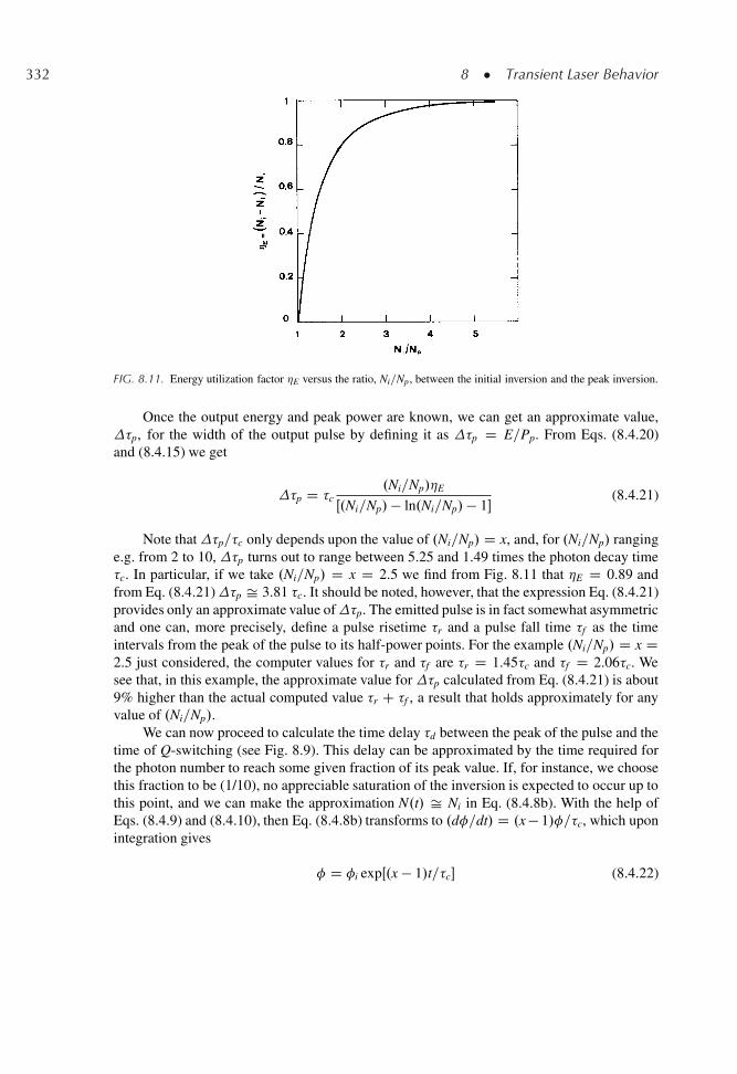
332 8 � Transient Laser Behavior
FIG. 8.11. Energy utilization factor �E versus the ratio, Ni=Np , between the initial inversion and the peak inversion.
Once the output energy and peak power are known, we can get an approximate value,�p, for the width of the output pulse by defining it as �p D E=Pp. From Eqs. (8.4.20)and (8.4.15) we get
�p D �c.Ni=Np/�E
Œ.Ni=Np/� ln.Ni=Np/� 1�(8.4.21)
Note that�p=�c only depends upon the value of .Ni=Np/ D x, and, for .Ni=Np/ ranginge.g. from 2 to 10, �p turns out to range between 5.25 and 1.49 times the photon decay time�c. In particular, if we take .Ni=Np/ D x D 2.5 we find from Fig. 8.11 that �E D 0.89 andfrom Eq. (8.4.21)�p Š 3.81 �c. It should be noted, however, that the expression Eq. (8.4.21)provides only an approximate value of�p. The emitted pulse is in fact somewhat asymmetricand one can, more precisely, define a pulse risetime �r and a pulse fall time �f as the timeintervals from the peak of the pulse to its half-power points. For the example .Ni=Np/ D x D2.5 just considered, the computer values for �r and �f are �r D 1.45�c and �f D 2.06�c. Wesee that, in this example, the approximate value for �p calculated from Eq. (8.4.21) is about9% higher than the actual computed value �r C �f , a result that holds approximately for anyvalue of .Ni=Np/.
We can now proceed to calculate the time delay �d between the peak of the pulse and thetime of Q-switching (see Fig. 8.9). This delay can be approximated by the time required forthe photon number to reach some given fraction of its peak value. If, for instance, we choosethis fraction to be (1/10), no appreciable saturation of the inversion is expected to occur up tothis point, and we can make the approximation N.t/ Š Ni in Eq. (8.4.8b). With the help ofEqs. (8.4.9) and (8.4.10), then Eq. (8.4.8b) transforms to .d�=dt/ D .x � 1/�=�c, which uponintegration gives
� D �i expŒ.x � 1/t=�c� (8.4.22)
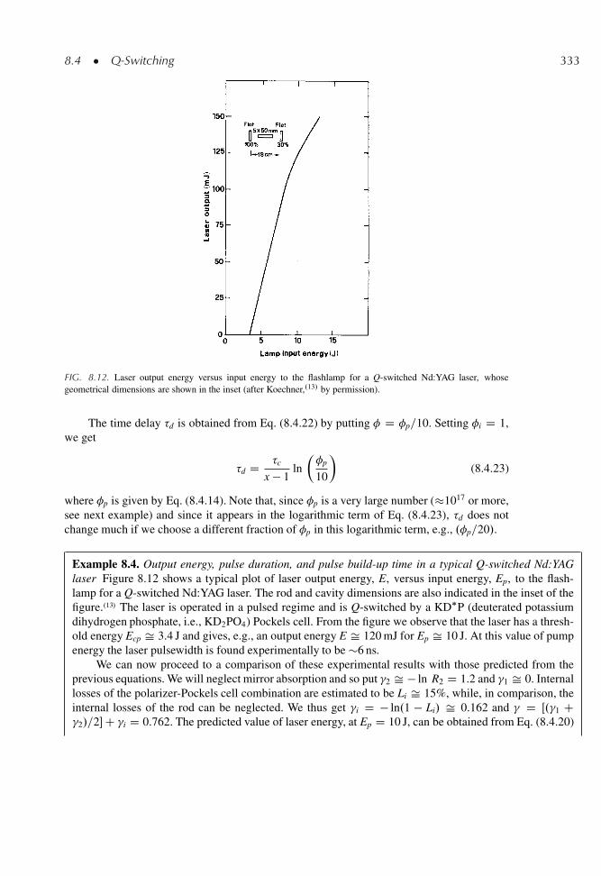
8.4 � Q-Switching 333
FIG. 8.12. Laser output energy versus input energy to the flashlamp for a Q-switched Nd:YAG laser, whosegeometrical dimensions are shown in the inset (after Koechner,.13/ by permission).
The time delay �d is obtained from Eq. (8.4.22) by putting � D �p=10. Setting �i D 1,we get
�d D �c
x � 1ln
��p
10
�(8.4.23)
where �p is given by Eq. (8.4.14). Note that, since �p is a very large number (�1017 or more,see next example) and since it appears in the logarithmic term of Eq. (8.4.23), �d does notchange much if we choose a different fraction of �p in this logarithmic term, e.g., .�p=20/.
Example 8.4. Output energy, pulse duration, and pulse build-up time in a typical Q-switched Nd:YAGlaser Figure 8.12 shows a typical plot of laser output energy, E, versus input energy, Ep, to the flash-lamp for a Q-switched Nd:YAG laser. The rod and cavity dimensions are also indicated in the inset of thefigure..13/ The laser is operated in a pulsed regime and is Q-switched by a KD�P (deuterated potassiumdihydrogen phosphate, i.e., KD2PO4) Pockels cell. From the figure we observe that the laser has a thresh-old energy Ecp Š 3.4 J and gives, e.g., an output energy E Š 120 mJ for Ep Š 10 J. At this value of pumpenergy the laser pulsewidth is found experimentally to be �6 ns.
We can now proceed to a comparison of these experimental results with those predicted from theprevious equations. We will neglect mirror absorption and so put �2 Š � ln R2 D 1.2 and �1 Š 0. Internallosses of the polarizer-Pockels cell combination are estimated to be Li Š 15%, while, in comparison, theinternal losses of the rod can be neglected. We thus get �i D � ln.1 � Li/ Š 0.162 and � D Œ.�1 C�2/=2�C �i D 0.762. The predicted value of laser energy, at Ep D 10 J, can be obtained from Eq. (8.4.20)
334 8 � Transient Laser Behavior
once we notice that, for our case, one has .Ni=Np/ D .Ep=Ecp/ D 2.9. We now assume Ab Š A D0.19 cm2, where A is the cross-sectional area of the rod. Since .Ni=Np/ D 2.9, we find from Fig. 8.11 that�E Š 0.94 and from Eq. (8.4.20), assuming an effective value of the stimulated emission cross section of� D 2.8 � 10�19 cm2 (see example 2.10), we obtain E Š 200 mJ. The somewhat larger value predictedby the theory can be attributed to two main reasons: (i) The area of the beam is certainly smaller than thatof the rod. (ii) Due to the short cavity length, the condition for fast switching, namely that the switchingtime is much shorter than the build-up time of the laser pulse, may not be well satisfied in our case. Lateron in this example, it will be shown, in fact, that the predicted build-up time of the Q-switched pulse,�d, is about 20 ns. It is difficult to switch the Pockels cell in a time much shorter than this value and, asa consequence, some energy will be lost, through the polarizer, during the switching process (in sometypical cases, with pulses of this short a duration, as much as 20% of the output energy can be found to beswitched out of the cavity by the polarizer, during the Q-switching process).
To calculate the predicted pulse duration we begin by noticing that, according to Eq. (7.2.11), theeffective resonator length is Le D L C .n � 1/l Š 22 cm, where n Š 1.83 for Nd:YAG, so that fromEq. (7.2.14) we obtain �c D Le=c� Š 1 ns. The laser pulsewidth is obtained through Eq. (8.4.21) as�p D �c�Ex=.x � ln x � 1/ Š 3.3 ns, where Fig. 8.11 has been used to calculate �E. The discrepancybetween this value and the experimental value, �p Š 6 ns, is attributed to two factors: (1) Multimodeoscillation. In fact, the build up time is expected to be different for different modes owing to their slightlydifferent gain and this should appreciably broaden the pulse duration. (2) As already mentioned, thecondition for fast switching may not be completely satisfied in our case, and the pulsewidth is expected tobe somewhat broadened by slow switching.
The build-up time of the Q-switched pulse can be obtained from Eq. (8.4.23) once �p is known. If wetake Np D �=� l Š 5.44 � 1017 cm�3 and assume Va D Ab l Š Al Š 1 cm3, from Eq. (8.4.14) we obtain�p Š 4.54 � 1017 photons, so that from Eq. (8.4.23), with �c D 1 ns and x D 2.9, we get �d Š 20 ns.
Example 8.5. Dynamical behavior of a passively Q-switched Nd:YAG laser We consider a laser cavitywith equivalent length Le D 50 cm in which the active medium is a Nd:YAG rod of diameter D D5 mm. We assume the laser to be passively Q-switched by a saturable absorber with saturation intensityIs D 1 MW=cm2 and we also assume that the cell containing the saturable absorber solution has anunsaturated loss of L D 50%. We take the output mirror reflectivity to be R2 D 74% and we neglect allother cavity losses. We thus have �2 D � ln R2 Š 0.3 for the loss of the output-coupling mirror and�a D � ln.1 � L/ D 0.693 for the unsaturated loss of the saturable absorber. The total unsaturated losswill then be �t D �a C .�2=2/ D 0.843. We now assume that the pump rate provides a square pulse lastingfor a time tP D 100 μs (see Fig. 8.13). According to Eq. (8.4.1) the population inversion, at the end of thepumping pulse and in the absence of laser action, is given by
N.tP/ D N1Œ1 � exp.�tP=�/� D 0.35N1 (8.4.24)
where we have taken � D 230 μs. Oscillation threshold will be reached at time tth (see Fig. 8.13) such that
�N.tth/l D �t (8.4.25)
8.4 � Q-Switching 335
We now set the pumping rate to exceed the laser threshold by 10% so that
N.tP/ D 1.1N.tth/ (8.4.26)
where N.tP/ is the inversion which would be present at t D tP in the absence of laser action (see Fig. 8.13).From Eqs. (8.4.26) and (8.4.24) we obtain N.tth/ Š 0.32 N1 so that, from Eq. (8.4.1), we get tth Š 88 μsand from Eq. (8.4.25) �N1l D �t=0.32 D 2.64.
For t > tth the laser will show a net gain, gnet.t0/, which, before appreciable absorber saturationoccurs, can be written as gnet.t/ D �Nl � �t Š � l.dN=dt/tht0, where we have changed to a new referencetime axis t0 whose origin is at t D tth. From Eq. (8.4.1) and using the previously calculated value of tth,one has .dN=dt/th D .N1=�/ exp.�tth=�/ D 0.68 .N1=�/. The net gain will then be given by gnet.t0/ D0.68.�N1l/.t0=�/ and, using the previously calculated value of .�N1l/, we get
gnet.t0/ Š 1.8.t0=�/ (8.4.27)
Once the expression for the net gain has been calculated, the growth of the cavity photons in the lasercavity can be obtained from the equation
.d�=dt/ D .gnet=tT/� (8.4.28)
where tT D Le=c Š 1.66 ns is the single-pass transit time for the laser cavity. Equation (8.4.28) could bereadily derived by an argument very similar to that used to obtain Eq. (7.2.12). If Eq. (8.4.27) is substitutedinto Eq. (8.4.28) and the resulting equation integrated, we obtain
�.t0/ D �i exp
"0.9
� tT�
� � t0
tT
�2#
(8.4.29)
Note that, since the net gain increases linearly with time [see Eq. (8.4.27)], �.t0/ increases exponen-tially with t02 [see Eq. (8.4.29) and see also Fig. 8.8a, where time t coincides with time t0 of this example].To calculate from Eq. (8.4.29) the time t0s at which saturation occurs, we need to relate �.t0/ to the circulat-ing beam intensity I.t0/. To arrive at this situation we first observe that, if two beams of the same intensity,I, are traveling in opposite directions within a laser cavity, the spatially averaged value of the energydensity within the cavity will be � D 2I=c [compare with Eq. (2.4.10)]. The relation between the photonnumber and the circulating laser intensity within the cavity will then be � D �AbLe=h� D 2IAbLe=ch�,where Ab is the beam area. From the previous expression, taking Ab D D2=4 Š 0.196 cm2, we find thatthe photon number �s corresponding to the saturation intensity, Is D 1 MW=cm2, is �s Š 3.49 � 1015.From Eq. (8.4.29), taking �i D 1, we then obtain .t0s=tT/ Š 2, 347 i.e., t0s Š 3.89 μs and hence ts Š 92 μs(see Fig. 8.13). Therefore, starting from the noise level, it takes �2,350 transits for the light to reach anintensity equal to the absorber saturation intensity. From this point on the saturable absorber bleaches veryrapidly.
For t > ts, the dynamical behavior of the laser can be calculated approximately by assuming that thesaturable absorber is completely bleached. The time evolution can then be obtained from the equations ofthis section by assuming, as initial inversion, Ni D N.ts/. We then have for the initial gain gi D �Nil D�N1lŒ1 � exp �.ts=�/� D 0.87, while the gain at the peak of the pulse is gp D �Npl D � D 0.15.We thus get Ni=Np D gi=gp D 5.8. The total initial inversion in the mode volume Va is then given by
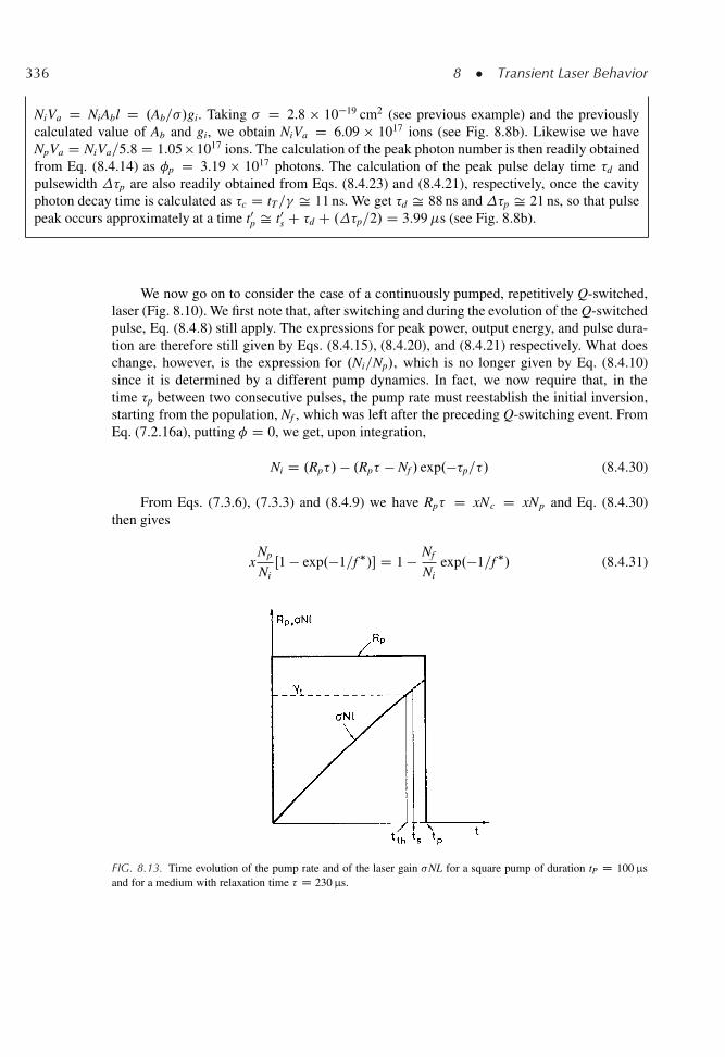
336 8 � Transient Laser Behavior
NiVa D NiAbl D .Ab=�/gi. Taking � D 2.8 � 10�19 cm2 (see previous example) and the previouslycalculated value of Ab and gi, we obtain NiVa D 6.09 � 1017 ions (see Fig. 8.8b). Likewise we haveNpVa D NiVa=5.8 D 1.05 � 1017 ions. The calculation of the peak photon number is then readily obtainedfrom Eq. (8.4.14) as �p D 3.19 � 1017 photons. The calculation of the peak pulse delay time �d andpulsewidth �p are also readily obtained from Eqs. (8.4.23) and (8.4.21), respectively, once the cavityphoton decay time is calculated as �c D tT=� Š 11 ns. We get �d Š 88 ns and �p Š 21 ns, so that pulsepeak occurs approximately at a time t0p Š t0s C �d C .�p=2/ D 3.99�s (see Fig. 8.8b).
We now go on to consider the case of a continuously pumped, repetitively Q-switched,laser (Fig. 8.10). We first note that, after switching and during the evolution of the Q-switchedpulse, Eq. (8.4.8) still apply. The expressions for peak power, output energy, and pulse dura-tion are therefore still given by Eqs. (8.4.15), (8.4.20), and (8.4.21) respectively. What doeschange, however, is the expression for .Ni=Np/, which is no longer given by Eq. (8.4.10)since it is determined by a different pump dynamics. In fact, we now require that, in thetime �p between two consecutive pulses, the pump rate must reestablish the initial inversion,starting from the population, Nf , which was left after the preceding Q-switching event. FromEq. (7.2.16a), putting � D 0, we get, upon integration,
Ni D .Rp�/ � .Rp� � Nf / exp.��p=�/ (8.4.30)
From Eqs. (7.3.6), (7.3.3) and (8.4.9) we have Rp� D xNc D xNp and Eq. (8.4.30)then gives
xNp
NiŒ1 � exp.�1=f �/� D 1 � Nf
Niexp.�1=f �/ (8.4.31)
FIG. 8.13. Time evolution of the pump rate and of the laser gain �NL for a square pump of duration tP D 100 μsand for a medium with relaxation time � D 230 μs.
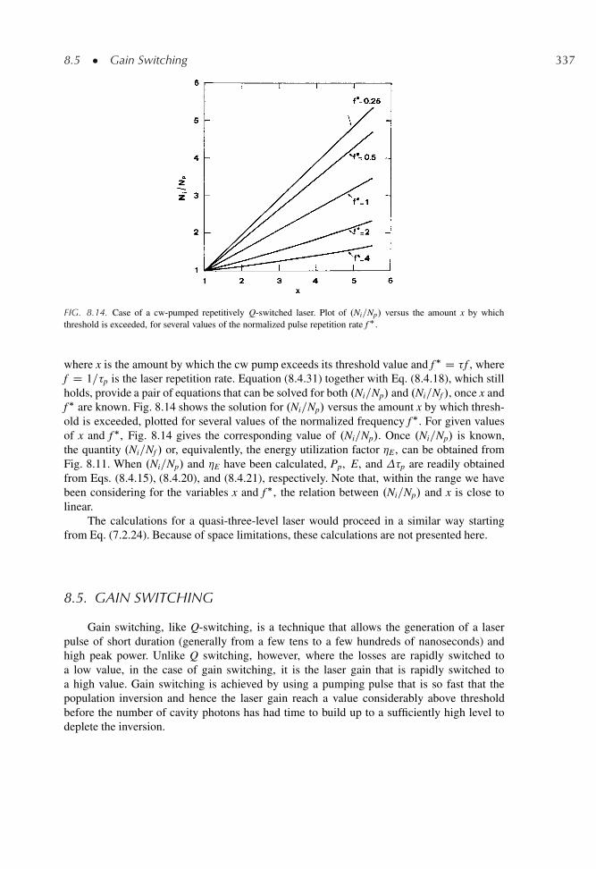
8.5 � Gain Switching 337
FIG. 8.14. Case of a cw-pumped repetitively Q-switched laser. Plot of .Ni=Np/ versus the amount x by whichthreshold is exceeded, for several values of the normalized pulse repetition rate f �.
where x is the amount by which the cw pump exceeds its threshold value and f � D � f , wheref D 1=�p is the laser repetition rate. Equation (8.4.31) together with Eq. (8.4.18), which stillholds, provide a pair of equations that can be solved for both .Ni=Np/ and .Ni=Nf /, once x andf � are known. Fig. 8.14 shows the solution for .Ni=Np/ versus the amount x by which thresh-old is exceeded, plotted for several values of the normalized frequency f �. For given valuesof x and f �, Fig. 8.14 gives the corresponding value of .Ni=Np/. Once .Ni=Np/ is known,the quantity .Ni=Nf / or, equivalently, the energy utilization factor �E , can be obtained fromFig. 8.11. When .Ni=Np/ and �E have been calculated, Pp, E, and �p are readily obtainedfrom Eqs. (8.4.15), (8.4.20), and (8.4.21), respectively. Note that, within the range we havebeen considering for the variables x and f �, the relation between .Ni=Np/ and x is close tolinear.
The calculations for a quasi-three-level laser would proceed in a similar way startingfrom Eq. (7.2.24). Because of space limitations, these calculations are not presented here.
8.5. GAIN SWITCHING
Gain switching, like Q-switching, is a technique that allows the generation of a laserpulse of short duration (generally from a few tens to a few hundreds of nanoseconds) andhigh peak power. Unlike Q switching, however, where the losses are rapidly switched toa low value, in the case of gain switching, it is the laser gain that is rapidly switched toa high value. Gain switching is achieved by using a pumping pulse that is so fast that thepopulation inversion and hence the laser gain reach a value considerably above thresholdbefore the number of cavity photons has had time to build up to a sufficiently high level todeplete the inversion.
338 8 � Transient Laser Behavior
The physical phenomena involved can be simply described by referring to the spikingsituation depicted in Fig. 8.1. If we assume that the pump rate, Rp D Rp.t/, is in the formof a square pulse starting at t D 0 and ending at t Š 5 μs, the light emission will consist ofjust the first spike of �.t/, occurring at about t D 5 μs. After this spike, in fact, the inversionwill have been driven by the light pulse to a value well below the threshold value and it doesnot grow thereafter as there is no further pumping. Thus we see that gain switching is similarin character to laser spiking described in Sect. 8.2. The main difference arises from the factthat, to obtain pulses of high peak power and short duration, the peak value of Rp must bemuch larger than the cw value considered in Fig. 8.1. Depending on the peak value of thispump rate, the peak inversion may then range between 4 and 10 times the threshold valuerather than the value of �1.48 shown in Fig. 8.1. The build up time of the laser radiation upto its peak value may correspondingly range between 5 and 20 times the cavity photon decaytime �c. The time duration of the pumping pulse must therefore be approximately equal to thisbuild-up time and hence very short..14/
In an actual situation, the time behavior of the pumping is usually in the form of a bell-shaped pulse rather than a square pulse. In this case we require that the peak of the photonspike occurs at an appropriate time in the trailing edge of the pumping pulse. In fact, if thispeak were to occur at e.g., the peak of the pumping pulse, there could be enough pump inputleft after the laser pulse to allow the inversion to exceed threshold again and thus produce asecond, although weaker, laser pulse. If, on the other hand, the photon peak were to occurmuch later in the tail of the pulse, this would imply that there was insufficient pumping timefor the inversion to grow to a sufficiently high value. The above discussion implies that, fora given duration of pump pulse, there is some optimum value for the peak pump rate. Bydecreasing the pump duration, the optimum value of the peak pump rate increases and a moreintense and narrower laser pulse is produced.
It should be noted that, given a sufficiently fast and intense pump pulse, any laser can inprinciple be gain switched even if the spontaneous decay of its upper laser level is allowedby electric dipole interaction and the lifetime correspondingly falls in the nanosecond range.In this case the pumping pulse and the cavity photon decay time must be appreciably shorterthan this lifetime and, correspondingly, very short gain switched pulses, i.e., with durationshorter than �1 ns, can be obtained.
Example 8.6. Typical cases of gain switched lasers The most common example of a gain-switched laseris the electrically pulsed TEA (Transversely Excited at Atmospheric pressure; see Chap. 10) CO2 laser.Taking a typical cavity length of L D 1 m, a 20% transmission of the output mirror, and assuming thatthe internal losses arise only from this mirror’s transmission, we get � Š 0.1 and �c D L=c� Š 30 ns.Assuming that the laser build up time is ten times longer, we see that the duration of the pumping pulseshould last �300 ns, in agreement with experimental findings.
As typical examples of gain switched lasers using active media with upper state lifetime, � , inthe nanosecond range, we mention the case of a short-cavity dye laser (e.g., Rhodamine 6G dye laser,� Š 5 ns) pumped by the fast .�0.5 ns/ pulse of an atmospheric pressure N2 laser or the case of a semi-conductor laser (e.g., GaAs, � Š 3 ns) pumped by a very short .�0.5 ns/ current pulse. In both cases, gainswitched laser pulses of �100 ps duration can be obtained.
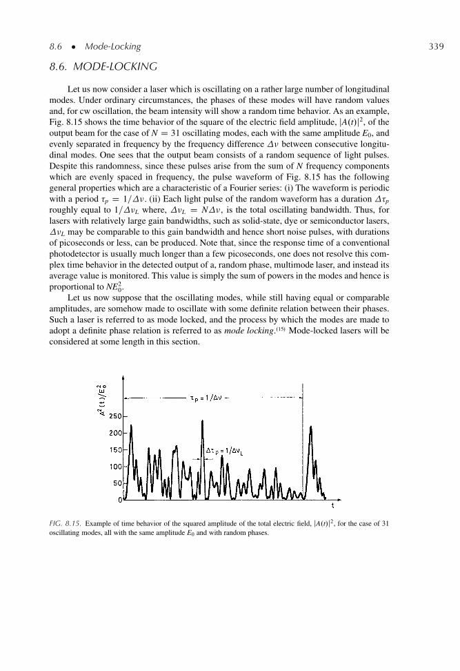
8.6 � Mode-Locking 339
8.6. MODE-LOCKING
Let us now consider a laser which is oscillating on a rather large number of longitudinalmodes. Under ordinary circumstances, the phases of these modes will have random valuesand, for cw oscillation, the beam intensity will show a random time behavior. As an example,Fig. 8.15 shows the time behavior of the square of the electric field amplitude, jA.t/j2, of theoutput beam for the case of N D 31 oscillating modes, each with the same amplitude E0, andevenly separated in frequency by the frequency difference � between consecutive longitu-dinal modes. One sees that the output beam consists of a random sequence of light pulses.Despite this randomness, since these pulses arise from the sum of N frequency componentswhich are evenly spaced in frequency, the pulse waveform of Fig. 8.15 has the followinggeneral properties which are a characteristic of a Fourier series: (i) The waveform is periodicwith a period �p D 1=�. (ii) Each light pulse of the random waveform has a duration �p
roughly equal to 1=�L where, �L D N�, is the total oscillating bandwidth. Thus, forlasers with relatively large gain bandwidths, such as solid-state, dye or semiconductor lasers,�L may be comparable to this gain bandwidth and hence short noise pulses, with durationsof picoseconds or less, can be produced. Note that, since the response time of a conventionalphotodetector is usually much longer than a few picoseconds, one does not resolve this com-plex time behavior in the detected output of a, random phase, multimode laser, and instead itsaverage value is monitored. This value is simply the sum of powers in the modes and hence isproportional to NE2
0.Let us now suppose that the oscillating modes, while still having equal or comparable
amplitudes, are somehow made to oscillate with some definite relation between their phases.Such a laser is referred to as mode locked, and the process by which the modes are made toadopt a definite phase relation is referred to as mode locking..15/ Mode-locked lasers will beconsidered at some length in this section.
FIG. 8.15. Example of time behavior of the squared amplitude of the total electric field, jA.t/j2, for the case of 31oscillating modes, all with the same amplitude E0 and with random phases.
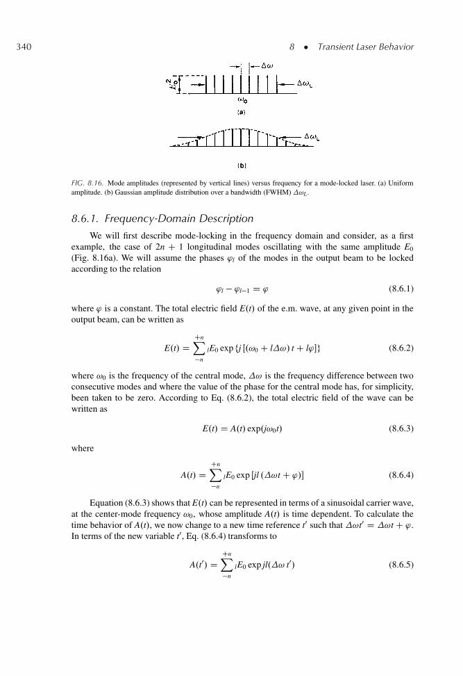
340 8 � Transient Laser Behavior
FIG. 8.16. Mode amplitudes (represented by vertical lines) versus frequency for a mode-locked laser. (a) Uniformamplitude. (b) Gaussian amplitude distribution over a bandwidth (FWHM) !L.
8.6.1. Frequency-Domain Description
We will first describe mode-locking in the frequency domain and consider, as a firstexample, the case of 2n C 1 longitudinal modes oscillating with the same amplitude E0
(Fig. 8.16a). We will assume the phases 'l of the modes in the output beam to be lockedaccording to the relation
'l � 'l�1 D ' (8.6.1)
where ' is a constant. The total electric field E.t/ of the e.m. wave, at any given point in theoutput beam, can be written as
E.t/ DCnX�n
lE0 exp fj Œ.!0 C l!/ t C l'�g (8.6.2)
where !0 is the frequency of the central mode, ! is the frequency difference between twoconsecutive modes and where the value of the phase for the central mode has, for simplicity,been taken to be zero. According to Eq. (8.6.2), the total electric field of the wave can bewritten as
E.t/ D A.t/ exp.j!0t/ (8.6.3)
where
A.t/ DCnX�n
lE0 exp Œjl .!t C '/� (8.6.4)
Equation (8.6.3) shows that E.t/ can be represented in terms of a sinusoidal carrier wave,at the center-mode frequency !0, whose amplitude A.t/ is time dependent. To calculate thetime behavior of A.t/, we now change to a new time reference t0 such that !t0 D !t C '.In terms of the new variable t0, Eq. (8.6.4) transforms to
A.t0/ DCnX�n
lE0 exp jl.! t0/ (8.6.5)
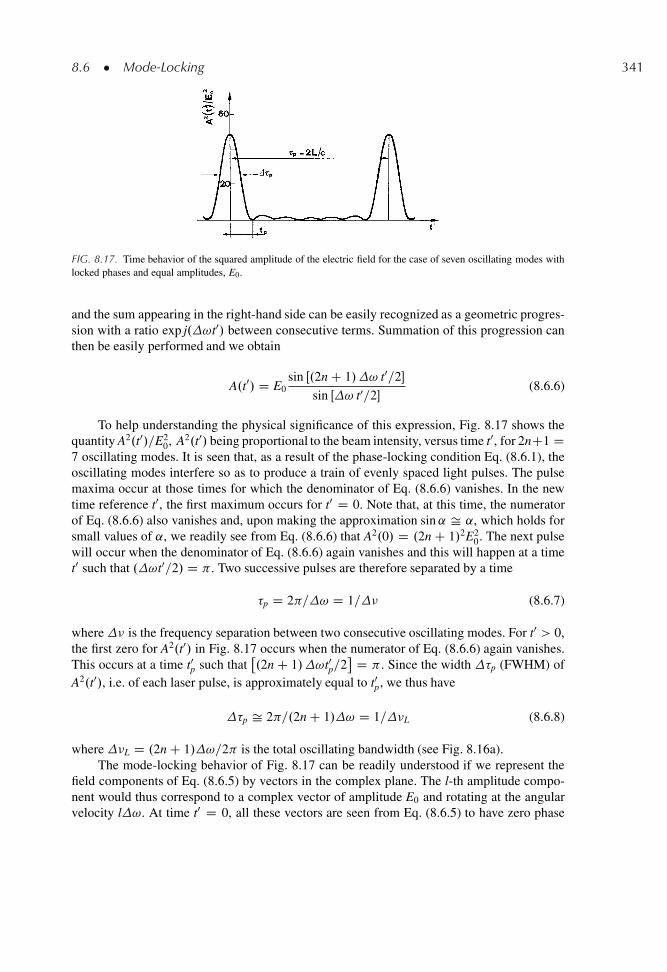
8.6 � Mode-Locking 341
FIG. 8.17. Time behavior of the squared amplitude of the electric field for the case of seven oscillating modes withlocked phases and equal amplitudes, E0.
and the sum appearing in the right-hand side can be easily recognized as a geometric progres-sion with a ratio exp j.!t0/ between consecutive terms. Summation of this progression canthen be easily performed and we obtain
A.t0/ D E0sin Œ.2n C 1/! t0=2�
sin Œ! t0=2�(8.6.6)
To help understanding the physical significance of this expression, Fig. 8.17 shows thequantity A2.t0/=E2
0, A2.t0/ being proportional to the beam intensity, versus time t0, for 2nC1 D7 oscillating modes. It is seen that, as a result of the phase-locking condition Eq. (8.6.1), theoscillating modes interfere so as to produce a train of evenly spaced light pulses. The pulsemaxima occur at those times for which the denominator of Eq. (8.6.6) vanishes. In the newtime reference t0, the first maximum occurs for t0 D 0. Note that, at this time, the numeratorof Eq. (8.6.6) also vanishes and, upon making the approximation sin ˛ Š ˛, which holds forsmall values of ˛, we readily see from Eq. (8.6.6) that A2.0/ D .2n C 1/2E2
0. The next pulsewill occur when the denominator of Eq. (8.6.6) again vanishes and this will happen at a timet0 such that .!t0=2/ D . Two successive pulses are therefore separated by a time
�p D 2 =! D 1=� (8.6.7)
where� is the frequency separation between two consecutive oscillating modes. For t0 > 0,the first zero for A2.t0/ in Fig. 8.17 occurs when the numerator of Eq. (8.6.6) again vanishes.This occurs at a time t0p such that
�.2n C 1/!t0p=2
D . Since the width �p (FWHM) ofA2.t0/, i.e. of each laser pulse, is approximately equal to t0p, we thus have
�p Š 2 =.2n C 1/! D 1=�L (8.6.8)
where �L D .2n C 1/!=2 is the total oscillating bandwidth (see Fig. 8.16a).The mode-locking behavior of Fig. 8.17 can be readily understood if we represent the
field components of Eq. (8.6.5) by vectors in the complex plane. The l-th amplitude compo-nent would thus correspond to a complex vector of amplitude E0 and rotating at the angularvelocity l!. At time t0 D 0, all these vectors are seen from Eq. (8.6.5) to have zero phase
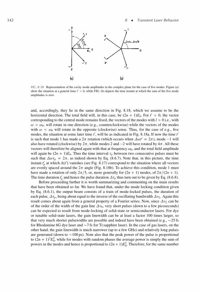
342 8 � Transient Laser Behavior
FIG. 8.18. Representation of the cavity mode amplitudes in the complex plane for the case of five modes. Figure (a)show the situation at a general time t0 > 0, while FIG. (b) depicts the time instant at which the sum of the five modeamplitudes is zero.
and, accordingly, they lie in the same direction in Fig. 8.18, which we assume to be thehorizontal direction. The total field will, in this case, be .2n C 1/E0. For t0 > 0, the vectorcorresponding to the central mode remains fixed, the vectors of the modes with l > 0 i.e., with! > !0, will rotate in one direction (e.g., counterclockwise) while the vectors of the modeswith ! < !0 will rotate in the opposite (clockwise) sense. Thus, for the case of e.g., fivemodes, the situation at some later time t0, will be as indicated in Fig. 8.18a. If now the time t0is such that mode 1 has made a 2 rotation (which occurs when !t0 D 2 ), mode �1 willalso have rotated (clockwise) by 2 , while modes 2 and �2 will have rotated by 4 . All thesevectors will therefore be aligned again with that at frequency !0, and the total field amplitudewill again be .2n C 1/E0. Thus the time interval �p between two consecutive pulses must besuch that !�p D 2 , as indeed shown by Eq. (8.6.7). Note that, in this picture, the timeinstant t0p at which A.t0/ vanishes (see Fig. 8.17) correspond to the situation where all vectorsare evenly spaced around the 2 angle (Fig. 8.18b). To achieve this condition, mode 1 musthave made a rotation of only 2 =5, or, more generally for .2n C 1/ modes, of 2 =.2n C 1/.The time duration t0p and hence the pulse duration�p thus turn out to be given by Eq. (8.6.8).
Before proceeding further it is worth summarizing and commenting on the main resultsthat have been obtained so far. We have found that, under the mode locking condition givenby Eq. (8.6.1), the output beam consists of a train of mode-locked pulses, the duration ofeach pulse,�p, being about equal to the inverse of the oscillating bandwidth�L. Again thisresult comes about again from a general property of a Fourier series. Now, since �L can beof the order of the width of the gain line �0, very short pulses (down to a few picoseconds)can be expected to result from mode-locking of solid-state or semiconductor lasers. For dyeor tunable solid-state lasers, the gain linewidth can be at least a factor 100 times larger, sothat very much shorter pulsewidths are possible and indeed have been obtained (e.g., �25 fsfor Rhodamine 6G dye laser and �7 fs for Ti:sapphire laser). In the case of gas lasers, on theother hand, the gain linewidth is much narrower (up to a few GHz) and relatively long pulsesare generated (down to �100 ps). Note also that the peak power of the pulse is proportionalto .2n C 1/2E2
0, while for modes with random phases the average power is simply the sum ofpowers in the modes and hence is proportional to .2n C 1/E2
0. Therefore, for the same number
8.6 � Mode-Locking 343
of oscillating modes and their field amplitudes E0, the ratio between the peak pulse powerin the mode-locked case and the average power in the non-mode-locked case is equal to thenumber, .2n C 1/, of oscillating modes, which, for solid state or liquid lasers, can be ratherhigh .103 � 104/. We thus see that mode-locking is useful not only for producing pulses ofvery short duration but also for producing high peak power.
So far we have restricted our considerations to the rather unrealistic case of an equal-amplitude mode-spectrum (Fig. 8.16a). In general the spectral envelope is expected to havea bell-shaped form and, as a characteristic example, we will consider an envelope with aGaussian distribution (Fig. 8.16b). We can therefore write the amplitude El of the l-th mode as
E2l D E2
0 exp
"��
2l!
!L
�2
ln 2
#(8.6.9)
where !L represents the bandwidth (FWHM) of the spectral intensity. If we again assumethat the phases are locked according to Eq. (8.6.1) and that the phase of the central mode isequal to zero, we again find that E.t/ can be expressed as in Eq. (8.6.3) where the amplitudeA.t/, in the time reference t0, is given by
A.t0/ DC1X�1
lEl exp j.l! t0/ (8.6.10)
If the sum is approximated by an integral [i.e., A.t/ Š REl exp j.l!t/dl], the field
amplitude A.t/ is seen to be proportional to the Fourier transform of the spectral amplitude El.We then find that A2.t/, i.e., the pulse intensity, is a Gaussian function of time, which can bewritten as
A2.t/ / exp
"��
2t
�p
�2
ln 2
#(8.6.11)
where
�p D 2 ln 2= �L D 0.441=�L (8.6.12)
Here, the term �p, appearing in Eq. (8.6.11), represents the width (FWHM) of the pulseintensity.
As a conclusion to our discussion of the two examples given above, we can say that, whenthe mode-locking condition Eq. (8.6.1) holds, the field amplitude turns out to be given by theFourier transform of the magnitude of the spectral amplitude. In such a case, the pulsewidth�p is related to the width of the laser spectrum �L by the relation �p D ˇ=�L, whereˇ is a numerical factor (of the order of unity), which depends on the particular shape of thespectral intensity distribution. A pulse of this sort is said to be transform-limited.
Under locking conditions different from Eq. (8.6.1), the output pulse may be far frombeing transform limited. As an example, instead of Eq. (8.6.1), which can be written as 'l Dl', we consider the situation where
'l D l'1 C l2'2 (8.6.13)
344 8 � Transient Laser Behavior
where '1 and '2 are two constants. If we again assume a Gaussian amplitude distribution suchas in Eq. (8.6.9), the Fourier transform of the spectrum can again be analytically calculatedand E.t/ can be written as
E.t/ / exp��˛t2
exp
�j!0t C ˇt2
�(8.6.14)
where the two constants ˛ and ˇ are related to !L and '2. For brevity, these relations arenot given here since they are not needed for what follows. What is important to notice here,however, are the following three points: (i) The beam intensity, being proportional to jE.t/j2,is still described by a Gaussian function whose pulsewidth �p (FWHM), in terms of theparameter ˛ is equal to
�p D .2 ln 2=˛/1=2 (8.6.15)
(ii) The presence of a phase term l2'2 in Eq. (8.6.13), which is quadratic in the mode indexl, results in E.t/ having a phase term, ˇt2, which is quadratic in time. This means that theinstantaneous carrier frequency of the wave, !.t/ D d.!0t C ˇt2/=dt D !0 C 2ˇt, nowhas a linear frequency sweep (or frequency chirp). (iii) Depending of the value of '2, theproduct �p�L can be much larger than the minimum value, 0.441, given by Eq. (8.6.12).To understand this point, it is easiest to go back to a calculation of the spectrum of a field suchas in Eq. (8.6.14). The spectral intensity again turns out to be given by a Gaussian functionwhose bandwidth�L (FWHM) is given by
�L D 0.441
�p
"1 C
ˇ�2
p
2 ln 2
!#1=2
(8.6.16)
where the expression for ˛ given by Eq. (8.6.15) has been used. Equation (8.6.16) shows that,if ˇ ¤ 0, one has �p�L > 0.441 and that, for ˇ�2
p � 1, i.e., for sufficiently large valuesof the frequency chirp, the product�p�L becomes much larger than 1. The physical basisfor this result can be understood by noting that the spectral broadening now arises both fromthe pulsed behavior of jE.t/j2, i.e., from the amplitude modulation of E.t/ [which accountsfor the first term on the right-hand side of Eq. (8.6.16)] and from the frequency chirp term 2ˇtof E.t/ [which accounts for the second term on the right-hand side of Eq. (8.6.16)].
8.6.2. Time-Domain Picture
We recall that, with the mode locking condition given by Eq. (8.6.1), two consecutivepulses of the output beam were found to be separated by a time �p given by Eq. (8.6.7). Since� D c=2L, where L is the cavity length, �p turns out to be equal to 2L=c, which is just thecavity round trip time. It should be noted at this point that the spatial extent z of a typicalmode-locked pulse is usually much shorter than the cavity length [e.g. for a pulse of duration�p D 1 ps, one has z D c�p D 0.3 mm while a laser cavity is typically several tens ofcentimeter long]. The oscillating behavior inside the laser cavity can therefore be visualized asconsisting of a single ultrashort pulse, of duration�p given by Eq. (8.6.8), which propagatesback and forth within the cavity. In such a case, in fact, the output beam would obviously
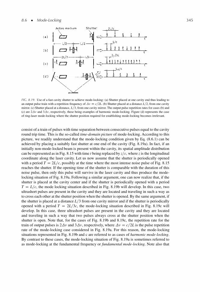
8.6 � Mode-Locking 345
FIG. 8.19. Use of a fast cavity shutter to achieve mode-locking: (a) Shutter placed at one cavity end thus leading toan output pulse train with a repetition frequency of � D c=2L. (b) Shutter placed at a distance L=2, from one cavitymirror. (c) Shutter placed at a distance, L=3, from one cavity mirror. The output pulse repetition rates for cases (b) and(c) are 2� and 3�, respectively, these being examples of harmonic mode-locking. Figure (d) represents the caseof ring-laser mode-locking where the shutter position required for establishing mode-locking becomes irrelevant.
consist of a train of pulses with time separation between consecutive pulses equal to the cavityround trip time. This is the so-called time-domain picture of mode-locking. According to thispicture, we readily understand that the mode-locking condition given by Eq. (8.6.1) can beachieved by placing a suitably fast shutter at one end of the cavity (Fig. 8.19a). In fact, if aninitially non-mode-locked beam is present within the cavity, its spatial amplitude distributioncan be represented as in Fig. 8.15 with time t being replaced by z=c, where z is the longitudinalcoordinate along the laser cavity. Let us now assume that the shutter is periodically openedwith a period T D 2L=c, possibly at the time where the most intense noise pulse of Fig. 8.15reaches the shutter. If the opening time of the shutter is comparable with the duration of thisnoise pulse, then only this pulse will survive in the laser cavity and thus produce the mode-locking situation of Fig. 8.19a. Following a similar argument, one can now realize that, if theshutter is placed at the cavity center and if the shutter is periodically opened with a periodT D L=c, the mode locking situation described in Fig. 8.19b will develop. In this case, twoultrashort pulses are present in the cavity and they are located and traveling in such a way asto cross each other at the shutter position when the shutter is opened. By the same argument, ifthe shutter is placed at a distance L=3 from one cavity mirror and if the shutter is periodicallyopened with a period T D 2L=3c, the mode-locking situation described in Fig. 8.19c willdevelop. In this case, three ultrashort pulses are present in the cavity and they are locatedand traveling in such a way that two pulses always cross at the shutter position when theshutter is open. Note that, for the cases of Fig. 8.19b and 8.19c, the repetition rate for thetrain of output pulses is 2� and 3�, respectively, where � D c=2L is the pulse repetitionrate of the mode-locking case considered in Fig. 8.19a. For this reason, the mode-lockingsituations represented in Fig. 8.19b and c are referred to as cases of harmonic mode-locking.By contrast to these cases, the mode-locking situation of Fig. 8.19a is sometimes referred toas mode-locking at the fundamental frequency or fundamental mode-locking. Note also that
346 8 � Transient Laser Behavior
the frequency domain description of mode-locking for the two cases of Fig. 8.19b and c mustcorrespond to a phase locking condition different from Eq. (8.6.1), since this condition wasshown to lead to the mode-locking picture of Fig. 8.19a. For instance, it can be shown that thephase locking condition corresponding to Fig. 8.19b is 'lC1 � 'l D 'l � 'l�1 C , instead of'lC1 � 'l D 'l � 'l�1 which is another form in which Eq. (8.6.1) can be expressed.
A rather interesting situation occurs when a ring laser cavity is used in mode-lockedoperation (Fig. 8.19d). In this case, independently of the shutter position within the cavity, thelaser will produce fundamental, second harmonic, or third harmonic mode-locking dependingon whether the shutter repetition rate is set equal to c=Lp, 2c=Lp, or 3c=Lp, where Lp isthe length of the ring cavity perimeter. For instance, assume that the shutter is opened witha repetition rate c=Lp (Fig. 8.19d). Then, if two counter-propagating pulses meet once atthe shutter position, they will then keep meeting at the same position after each round trip,independently of shutter position.
8.6.3. Methods of Mode-Locking
The methods of mode-locking, like those of Q-switching, can be divided into two cate-gories: (1) Active-mode-locking, in which the mode-locking element is driven by an externalsource. (2) Passive mode-locking, in which the element which induces mode-locking is notdriven externally and instead exploits some non-linear optical effect such as saturation of asaturable absorber or non-linear refractive index change of a suitable material.
8.6.3.1. Active Mode-Locking
There are three main types of active mode-locking (ML), namely: (1) Mode-lockinginduced by an amplitude modulator (AM mode-locking). (2) Mode-locking induced by aphase modulator (FM mode-locking). (3) Mode-locking induced by a periodic modulationof the laser gain at a repetition rate equal to the fundamental cavity frequency � D c=2L(ML by synchronous pumping). We will discuss AM mode-locking in most details, this typebeing the most popular, and then give a briefer discussion of the FM mode-locking. Mode-locking by synchronous pumping will not be discussed here since it is now less widely used.In fact, it only applies to active media with nanosecond relaxation time, notably dye media,and, to obtain the shortest pulses, requires that the modulation rate of the pump be equal, towithin high precision, to the fundamental frequency of the laser cavity. For this reason, pulsedurations shorter than 1 ps are difficult to achieve from a synchronously pumped dye laser.
To describe AM-mode-locking, we suppose a modulator to be inserted in the cavity,which produces a time-varying loss at frequency !m. If !m ¤ !, where ! D 2 �, �being the frequency difference between longitudinal modes, this loss will simply amplitudemodulate the electric field, El.t/, of each cavity mode to give
El.t/ D E0Œ1 � .ı=2/.1 � cos!mt/� cos.!lt C �l/ (8.6.17)
where !l is the mode frequency, �l its phase and where ı is the depth of amplitude modula-tion, which means that the field amplitude is modulated from E0 to E0.1 � ı/. Note that theterm E0.ı=2/ cos!mt�cos.!l tC�l/ in Eq. (8.6.17) can be written as .E0ı=4/fcosŒ.!l C!m/t
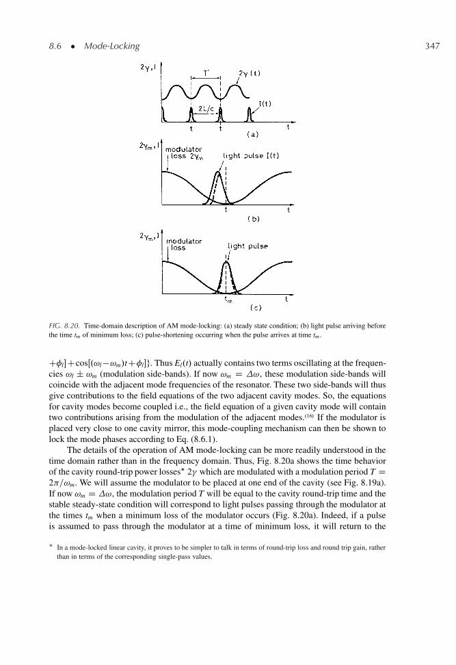
8.6 � Mode-Locking 347
FIG. 8.20. Time-domain description of AM mode-locking: (a) steady state condition; (b) light pulse arriving beforethe time tm of minimum loss; (c) pulse-shortening occurring when the pulse arrives at time tm .
C�l�CcosŒ.!l �!m/tC�l�g. Thus El.t/ actually contains two terms oscillating at the frequen-cies !l ˙ !m (modulation side-bands). If now !m D !, these modulation side-bands willcoincide with the adjacent mode frequencies of the resonator. These two side-bands will thusgive contributions to the field equations of the two adjacent cavity modes. So, the equationsfor cavity modes become coupled i.e., the field equation of a given cavity mode will containtwo contributions arising from the modulation of the adjacent modes..16/ If the modulator isplaced very close to one cavity mirror, this mode-coupling mechanism can then be shown tolock the mode phases according to Eq. (8.6.1).
The details of the operation of AM mode-locking can be more readily understood in thetime domain rather than in the frequency domain. Thus, Fig. 8.20a shows the time behaviorof the cavity round-trip power losses� 2� which are modulated with a modulation period T D2 =!m. We will assume the modulator to be placed at one end of the cavity (see Fig. 8.19a).If now !m D !, the modulation period T will be equal to the cavity round-trip time and thestable steady-state condition will correspond to light pulses passing through the modulator atthe times tm when a minimum loss of the modulator occurs (Fig. 8.20a). Indeed, if a pulseis assumed to pass through the modulator at a time of minimum loss, it will return to the
� In a mode-locked linear cavity, it proves to be simpler to talk in terms of round-trip loss and round trip gain, ratherthan in terms of the corresponding single-pass values.
348 8 � Transient Laser Behavior
modulator after a time, 2L=c, where the loss is again at a minimum. If, on the other hand, thepulse is assumed to initially pass through the modulator at a time, e.g., slightly shorter thantm (solid-line pulse in Fig. 8.20b), then the effect of the time-varying loss of the modulatoris that the leading edge of the pulse will suffer more attenuation than the trailing edge. Thus,after passing through the modulator, the pulse indicated by a dashed line in Fig. 8.20b willresult, having its pulse peak advanced in such a way that, during the next passage, the peakwill arrive closer to tm. This shows that, eventually, the steady state situation of Fig. 8.20awill be reached. Actually, in this case, the pulse-duration tends to be shortened each time thepulse passes through the modulator because both the leading and trailing edge of the pulse aresomewhat attenuated while the peak of the pulse is not attenuated by the time varying loss,2�m.t/, of the modulator (see Fig. 8.20c). Thus, if it were only for this mechanism, the pulse-duration would tend to zero with progressive passages through the modulator. This is howeverprevented by the finite bandwidth of the gain medium. In fact, as the pulse becomes shorter,its spectrum would eventually become so large to fill the bandwidth of the laser medium.The wings of the pulse spectrum would then no longer be amplified. This constitutes thefundamental limitation to the pulse bandwidth and hence to the pulse duration.
The way in which the finite bandwidth of the active medium influences the steady-state pulse duration is quite different, however, for homogeneous or inhomogeneous lines.For an inhomogeneously broadened line and if the laser is sufficiently far above threshold,the oscillating bandwidth �L tends to cover the whole gain bandwidth ��
0 . In fact, in afrequency-domain description, the primary purpose of the modulator is to lock the phasesof these already oscillating modes. Under the synchronism condition, !m D !, and if theAM modulator is placed at one cavity end, the phase locking condition given by Eq. (8.6.1)develops and, assuming for simplicity a Gaussian distribution for the mode amplitudes, weget from Eq. (8.6.12).
�p Š 0.441=��0 (8.6.18)
By contrast to this situation, for a homogeneous line, the phenomenon of spatial holeburning tends to concentrate the width of the oscillating spectrum in a narrow region aroundthe central frequency �0 (see Sect. 7.7). Thus, assuming the laser to be originally unlocked,the noise light pulses (see Fig. 8.15) would tend to be appreciably longer than 1=�0, where�0 is the width of the gain line. In this case, the mechanism described in Fig. 8.20c is reallyeffective in shortening the pulse duration, i.e., in broadening its spectrum. This pulse narrow-ing is however counteracted by pulse broadening occurring when the pulse passes through theactive medium and so undergoes spectral narrowing. The theory of active mode-locking, for ahomogeneously broadened gain medium, has been given a detailed and elegant treatment byKuizenga and Siegman.17/ and, later, presented in a more general framework by Haus..18/ Wewill limit ourselves here to just quoting the most relevant results and refer to Appendix F fora more detailed treatment. The intensity profile turns out to be well described by a Gaussianfunction whose width �p (FWHM) is approximately given by
�p Š 0.45=.�m�0/1=2 (8.6.19)
where �m is the frequency of the modulator (�m D !m=2 D c=2L, for fundamental har-monic mode-locking). If the pulsewidth expressions for inhomogeneous, Eq. (8.6.18), and
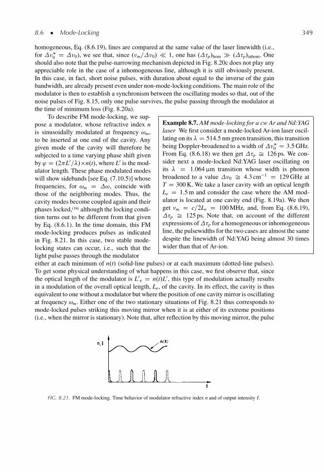
8.6 � Mode-Locking 349
homogeneous, Eq. (8.6.19), lines are compared at the same value of the laser linewidth (i.e.,for ��
0 D �0), we see that, since .�m=�0/ � 1, one has .�p/hom � .�p/inhom. Oneshould also note that the pulse-narrowing mechanism depicted in Fig. 8.20c does not play anyappreciable role in the case of a inhomogeneous line, although it is still obviously present.In this case, in fact, short noise pulses, with duration about equal to the inverse of the gainbandwidth, are already present even under non-mode-locking conditions. The main role of themodulator is then to establish a synchronism between the oscillating modes so that, out of thenoise pulses of Fig. 8.15, only one pulse survives, the pulse passing through the modulator atthe time of minimum loss (Fig. 8.20a).
Example 8.7. AM mode-locking for a cw Ar and Nd:YAGlaser We first consider a mode-locked Ar-ion laser oscil-lating on its � D 514.5 nm green transition, this transitionbeing Doppler-broadened to a width of ��
0 D 3.5 GHz.From Eq. (8.6.18) we then get �p Š 126 ps. We con-sider next a mode-locked Nd:YAG laser oscillating onits � D 1.064 μm transition whose width is phononbroadened to a value �0 Š 4.3 cm�1 D 129 GHz atT D 300 K. We take a laser cavity with an optical lengthLe D 1.5 m and consider the case where the AM mod-ulator is located at one cavity end (Fig. 8.19a). We thenget �m D c=2Le D 100 MHz, and, from Eq. (8.6.19),�p Š 125 ps. Note that, on account of the differentexpressions of�p for a homogeneous or inhomogeneousline, the pulsewidths for the two cases are almost the samedespite the linewidth of Nd:YAG being almost 30 timeswider than that of Ar-ion.
To describe FM mode-locking, we sup-pose a modulator, whose refractive index nis sinusoidally modulated at frequency !m,to be inserted at one end of the cavity. Anygiven mode of the cavity will therefore besubjected to a time varying phase shift givenby ' D .2 L0=�/�n.t/, where L0 is the mod-ulator length. These phase modulated modeswill show sidebands [see Eq. (7.10.5)] whosefrequencies, for !m D !, coincide withthose of the neighboring modes. Thus, thecavity modes become coupled again and theirphases locked,.16/ although the locking condi-tion turns out to be different from that givenby Eq. (8.6.1). In the time domain, this FMmode-locking produces pulses as indicatedin Fig. 8.21. In this case, two stable mode-locking states can occur, i.e., such that thelight pulse passes through the modulatoreither at each minimum of n.t/ (solid-line pulses) or at each maximum (dotted-line pulses).To get some physical understanding of what happens in this case, we first observe that, sincethe optical length of the modulator is L0
e D n.t/L0, this type of modulation actually resultsin a modulation of the overall optical length, Le, of the cavity. In its effect, the cavity is thusequivalent to one without a modulator but where the position of one cavity mirror is oscillatingat frequency !m. Either one of the two stationary situations of Fig. 8.21 thus corresponds tomode-locked pulses striking this moving mirror when it is at either of its extreme positions(i.e., when the mirror is stationary). Note that, after reflection by this moving mirror, the pulse
FIG. 8.21. FM mode-locking. Time behavior of modulator refractive index n and of output intensity I.
350 8 � Transient Laser Behavior
will acquire a nearly parabolic phase variation, of either positive sign (for the solid-line pulses)or negative sign (for the dotted-line pulses), and its spectrum will be slightly broadened.The overall phase modulation of the pulse and the corresponding pulse duration will thenbe established by the condition that the spectral broadening produced at each reflection fromthe moving mirror must be compensated by the spectral narrowing resulting from the passagethrough the amplifier. A stability analysis could also be performed to understand what happenswhen the pulse strikes the mirror not exactly at a stationary point. However, this analysis turnsout to be rather complicated and, due to the somewhat limited importance of this type of mode-locking, it will not be considered here. In fact, this type of locking is much less frequentlyused in practice for two main reasons: (i) The pulses are frequency modulated. (ii) Mode-locking tends to be somewhat unstable in the sense that switching between the two states ofFig. 8.21 often occurs in practice.
For a pulsed and generally high gain laser, AM mode-locking is commonly achieved bya Pockels cell amplitude modulator. A possible configuration may be that shown in Fig. 8.5awith the Pockels cell voltage being sinusoidally modulated from zero to some fraction of the�=4 voltage. For a cw pumped and generally low gain laser, AM mode-locking is more com-monly achieved with an acousto-optic modulator, owing to its lower insertion loss comparedto a Pockels cell modulator. However, the acousto-optic modulator used for mode-lockingdiffers significantly from that used for Q-switching and discussed in Fig. 8.7. In fact, the faceto which the piezoelectric transducer is bonded and the opposite face of the optical materialare now cut parallel each other. The sound wave launched into the material by the transduceris then reflected back by the opposite face of the material. So, if the length of the optical blockis equal to an integral number of half-wavelengths of the sound wave, an acoustic standing-wave pattern is produced. Since the amplitude of the standing-wave is sinusoidally modulatedin time, the same will happen for the diffraction losses. It can be shown, however, that, if thesound wave is oscillating at frequency !, the diffraction loss will be modulated at frequency2!. Consider, in fact, an acoustic standing-wave of the form S D S0 .cos!t/.sin kz/. Themodulator loss will reaches a maximum whenever a maximum amplitude of the standing-wave pattern occurs and this maximum is reached twice in an oscillation period (i.e., at t D 0and t D =!). The modulator loss is thus modulated at frequency 2! and, for fundamentalML (see Fig. 8.19a), ML is achieved when: (i) the modulator is put as near as possible to onecavity mirror; (ii) the modulation frequency 2� is set equal to .c=2L/ and, accordingly, thetransducer is driven at a frequency equal to c=4L (e.g., � D 50 MHz for L D 1.5 m). In thecase of FM mode-locking (both for pulsed or cw lasers), a Pockels cell electro-optic phasemodulator is commonly used. In this case one of the two axes, e.g., x, of induced birefrin-gence (see Fig. 8.5b) is oriented along the polarizer axis. So, the beam does not rotate itspolarization when passing through the Pockels cell but, rather, acquires a phase shift givenby � D .2 L0=�/nx, where L0 is the Pockels cell length and nx is its refractive index forpolarization along x-direction. If now the voltage to the Pockels is sinusoidally modulated,the refractive index nx, due to the Pockels effect, will also be sinusoidally modulated and thesame modulation will occur to the phase of the beam.
8.6.3.2. Passive Mode Locking
There are four main types of passive mode-locking (ML), namely: (1) Fast saturableabsorber ML, which makes use of the saturation properties of a suitable absorber (e.g.a dye molecule or a semiconductor) with very short upper state lifetime. (2) Kerr Lens
8.6 � Mode-Locking 351
Mode-locking (KLM), which exploits the self-focusing property of a suitable transparentnon-linear optical material. (3) Slow saturable absorber ML, which exploits the dynamicsaturation of the gain medium. (4) Additive Pulse ML (APM), in which one exploits the self-phase-modulation induced in a suitable non-linear optical element inserted in an auxiliarycavity, coupled to the main cavity and of identical length. In this case, the pulse shorteningmechanism arises from the interference of the main pulse in the laser cavity with the pulsecoupled back from the auxiliary cavity and which has been phase-modulated by the non-linear material. APM locking requires however that the optical lengths of the two cavitiesbe equal with an accuracy typically of a fraction of the laser wavelength. For this reason,this type of ML is not so widely used as the other techniques and will not be discussedfurther here.
To illustrate mode-locking by a fast saturable absorber, we consider an absorber withlow saturation intensity and with relaxation time much shorter than the duration of the mode-locked pulses. The theory of mode-locking by a fast saturable absorber, for a homogeneouslybroadened gain medium, has been treated in detail, notably by Haus..19/ We will only quotehere the most relevant results and refer to Appendix F for a more detailed treatment.
For low values of intracavity beam intensity, I, compared to the absorber’s saturationintensity, Is, the cavity round-trip power-loss� can be written as
2�t D 2� � 2� 0.I = Is/ (8.6.20)
where � is the unsaturable single-pass loss and � 0 is the low-intensity single-pass loss ofthe saturable absorber�. Suppose now that the absorber is very thin and placed in contactwith one cavity mirror (Fig. 8.19a) and that the laser is initially oscillating with mode phasesun-locked. The intensity of each of the two traveling waves will be made up of a randomsequence of light bursts (see Fig. 8.15) and, for the initially low peak intensity of these bursts,the saturated round-trip power gain, 2g0, will be roughly equal to the cavity unsaturable loss.However, the most intense pulse of Fig. 8.15, as a result of absorber saturation, will suffer theleast attenuation in the saturable absorber. If certain special conditions are met,.19/ this pulsecan then grow faster than the others and, after many round trips, the situation described inFig. 8.22 will eventually be established, where, for simplicity, the gain medium and saturableabsorber are assumed to be together at one end of the cavity. In this case a single, intense, MLpulse survives in the cavity and, due to the reduced loss arising from the more pronouncedabsorber saturation, the average power will increase compared to the unlocked case and, cor-respondingly, the round-trip saturated gain, 2g0
0, will now become smaller than the round-tripunsaturable loss of the cavity. Accordingly, a time window of net gain is established duringthe passage of the pulse, i.e., between times t1 and t2 in the figure, the pulse tails seeing a netloss and the pulse peak a net gain. If it were only for this mechanism, the pulse would be pro-gressively shortened after each pass through the absorber-amplifier combination. However,a steady state condition is again established by the balance between this pulse shortening
� In a mode-locked linear cavity it is preferable to think in terms of round-trip loss and gain rather than in terms ofthe corresponding single-pass values
� According to (2.8.12) and for I Is, the absorbance, �a , of an absorber of length la can be written as �a D ˛la D˛0 laŒ1 � .I=Is/� and the intensity independent term ˛0 la can be included in the total unsaturable loss � .
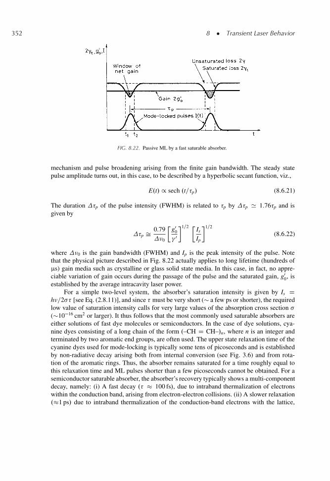
352 8 � Transient Laser Behavior
FIG. 8.22. Passive ML by a fast saturable absorber.
mechanism and pulse broadening arising from the finite gain bandwidth. The steady statepulse amplitude turns out, in this case, to be described by a hyperbolic secant function, viz.,
E.t/ / sech .t=�p/ (8.6.21)
The duration �p of the pulse intensity (FWHM) is related to �p by �p ' 1.76�p and isgiven by
�p Š 0.79
�0
�g0
0
� 0
�1=2 � Is
Ip
�1=2
(8.6.22)
where �0 is the gain bandwidth (FWHM) and Ip is the peak intensity of the pulse. Notethat the physical picture described in Fig. 8.22 actually applies to long lifetime (hundreds ofμs) gain media such as crystalline or glass solid state media. In this case, in fact, no appre-ciable variation of gain occurs during the passage of the pulse and the saturated gain, g0
0, isestablished by the average intracavity laser power.
For a simple two-level system, the absorber’s saturation intensity is given by Is Dh�=2�� [see Eq. (2.8.11)], and since � must be very short (� a few ps or shorter), the requiredlow value of saturation intensity calls for very large values of the absorption cross section �(�10�16 cm2 or larger). It thus follows that the most commonly used saturable absorbers areeither solutions of fast dye molecules or semiconductors. In the case of dye solutions, cya-nine dyes consisting of a long chain of the form .–CH D CH–/n, where n is an integer andterminated by two aromatic end groups, are often used. The upper state relaxation time of thecyanine dyes used for mode-locking is typically some tens of picoseconds and is establishedby non-radiative decay arising both from internal conversion (see Fig. 3.6) and from rota-tion of the aromatic rings. Thus, the absorber remains saturated for a time roughly equal tothis relaxation time and ML pulses shorter than a few picoseconds cannot be obtained. For asemiconductor saturable absorber, the absorber’s recovery typically shows a multi-componentdecay, namely: (i) A fast decay .� � 100 fs/, due to intraband thermalization of electronswithin the conduction band, arising from electron-electron collisions. (ii) A slower relaxation.�1 ps/ due to intraband thermalization of the conduction-band electrons with the lattice,
8.6 � Mode-Locking 353
arising from electron-phonon collisions. (iii) A still slower relaxation (from a few picosec-onds to some nanoseconds) due to interband radiative and non-radiative decay. The longestrelaxation time will result in the lowest saturation intensity, and this is helpful for starting theML process. The fastest relaxation time then provides the fast saturable absorber mechanismneeded to produce short pulses. A particularly interesting solution consists in integrating amultiple-quantum-well saturable absorber between two mirrors whose spacing is such thatthe resulting Fabry-Perot etalon operates at anti-resonance, i.e., at a point where a minimumof transmission or a maximum of reflection occurs (see Fig. 4.11). If the etalon is used asone cavity mirror, the laser intensity within the etalon may be substantially reduced com-pared to the value of the laser cavity. This offers the considerable advantages of increasing,in a controlled manner, the effective value of the saturation intensity, decreasing the effectiveunsaturable losses, and increasing the damage threshold..20/ The effectiveness of this simple-to-use anti-resonance-Fabry-Perot-saturable absorber (A-FPSA) has been widely proven forgenerating both picosecond and femtosecond laser pulses from several wide-bandwidth solidstate lasers.
Example 8.8. Passive mode-locking of a Nd:YAG andNd:YLF laser by a fast saturable absorber We considera cw Nd:YAG laser passively mode-locked by a �0.6 μmthick multiple-quantum-well (�50 wells) InGaAs/GaAsA-FPSA..20/ We take g0
0 D 2%, � 0 D 1%, �0 D4.5 cm�1 Š 135 GHz at T D 300 K, and Ip D 0.3 Is.From Eq. (8.6.22) we then get �p Š 15 ps. Notethat, in this case, the absorber is heavily saturated andEq. (8.6.22) can only be taken as a first order approx-imation to the calculation of the predicted pulse-width.For the case of a Nd:YLF laser, we will assume thesame value of the unsaturable and saturable losses asfor Nd:YAG. We therefore assume the same value ofg0
0. The gain linewidth of Nd:YLF, �00, is taken to be
about three-times larger than that of Nd:YAG (i.e.,�00 Š
13 cm�1) and the comparison then made at the samevalue of output power i.e., at the same value of thepulse energy E Š Ip �p. From Eq. (8.6.22) one read-ily finds that the pulsewidth � 0
p for this case is relatedto the pulsewidth of the previous case by the relation� 0
p D �0=�
00
�2�p. For � 0
0 D 2.89�0 we thenget � 0
p Š 1.8 ps. Note the strong dependence of laserpulsewidth on gain linewidth under these conditions.
Another fast passive mode-locking tech-nique relies on the lens-effect induced in asuitable material by a Kerr-type non-linearityand is thus referred to as Kerr-Lens-Mode-Locking (KLM)..21,22/ Consider first an opti-cal material, such as quartz or sapphire, tra-versed by a light beam of uniform intensityI. At sufficiently high intensity, the refractiveindex of the medium will be influenced to areadily observable extent by the field inten-sity, i.e., one can generally write n D n.I/.The first term of a Taylor expansion of nvs I will be proportional to I and one canthus write
n D n0 C n2I (8.6.23)
where n2 is a positive coefficient whichdepends on the material (e.g. n2 Š 4.5 �10�16 cm2=W for fused quartz and n2 Š3.45 � 10�16 cm2=W for sapphire). This phe-nomenon is known as the optical Kerr effectand is generally due to a hyper-polarizabilityof the medium occurring at high electricfields and arising from either a deformationof the electronic orbitals of the atoms or molecules or from a reorientation of the molecules(for a gas or liquid). For a solid, only deformation of the atom’s electron cloud can occurand the optical Kerr effect is very fast, the response time being of the order of a rotationperiod of the outermost electrons of the atom (a few femtoseconds). Assume now that thebeam intensity, in a medium exhibiting the optical Kerr effect (a Kerr medium), has a giventransverse profile, e.g., Gaussian. The intensity at the beam center will then be larger than in
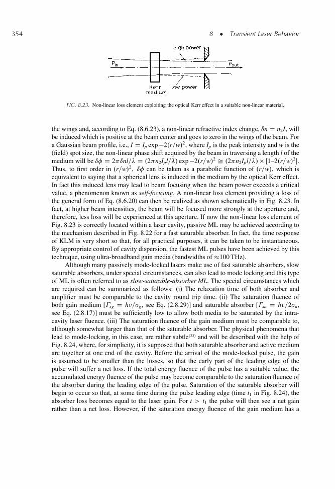
354 8 � Transient Laser Behavior
FIG. 8.23. Non-linear loss element exploiting the optical Kerr effect in a suitable non-linear material.
the wings and, according to Eq. (8.6.23), a non-linear refractive index change, ın D n2I, willbe induced which is positive at the beam center and goes to zero in the wings of the beam. Fora Gaussian beam profile, i.e., I D Ip exp �2.r=w/2, where Ip is the peak intensity and w is the(field) spot size, the non-linear phase shift acquired by the beam in traversing a length l of themedium will be ı� D 2 ınl=� D .2 n2Ipl=�/ exp �2.r=w/2 Š .2 n2Ipl=�/ � Œ1–2.r=w/2�.Thus, to first order in .r=w/2, ı� can be taken as a parabolic function of .r=w/, which isequivalent to saying that a spherical lens is induced in the medium by the optical Kerr effect.In fact this induced lens may lead to beam focusing when the beam power exceeds a criticalvalue, a phenomenon known as self-focusing. A non-linear loss element providing a loss ofthe general form of Eq. (8.6.20) can then be realized as shown schematically in Fig. 8.23. Infact, at higher beam intensities, the beam will be focused more strongly at the aperture and,therefore, less loss will be experienced at this aperture. If now the non-linear loss element ofFig. 8.23 is correctly located within a laser cavity, passive ML may be achieved according tothe mechanism described in Fig. 8.22 for a fast saturable absorber. In fact, the time responseof KLM is very short so that, for all practical purposes, it can be taken to be instantaneous.By appropriate control of cavity dispersion, the fastest ML pulses have been achieved by thistechnique, using ultra-broadband gain media (bandwidths of �100 THz).
Although many passively mode-locked lasers make use of fast saturable absorbers, slowsaturable absorbers, under special circumstances, can also lead to mode locking and this typeof ML is often referred to as slow-saturable-absorber ML. The special circumstances whichare required can be summarized as follows: (i) The relaxation time of both absorber andamplifier must be comparable to the cavity round trip time. (ii) The saturation fluence ofboth gain medium [�sg D h�=�g, see Eq. (2.8.29)] and saturable absorber [�sa D h�=2�a,see Eq. (2.8.17)] must be sufficiently low to allow both media to be saturated by the intra-cavity laser fluence. (iii) The saturation fluence of the gain medium must be comparable to,although somewhat larger than that of the saturable absorber. The physical phenomena thatlead to mode-locking, in this case, are rather subtle.23/ and will be described with the help ofFig. 8.24, where, for simplicity, it is supposed that both saturable absorber and active mediumare together at one end of the cavity. Before the arrival of the mode-locked pulse, the gainis assumed to be smaller than the losses, so that the early part of the leading edge of thepulse will suffer a net loss. If the total energy fluence of the pulse has a suitable value, theaccumulated energy fluence of the pulse may become comparable to the saturation fluence ofthe absorber during the leading edge of the pulse. Saturation of the saturable absorber willbegin to occur so that, at some time during the pulse leading edge (time t1 in Fig. 8.24), theabsorber loss becomes equal to the laser gain. For t > t1 the pulse will then see a net gainrather than a net loss. However, if the saturation energy fluence of the gain medium has a
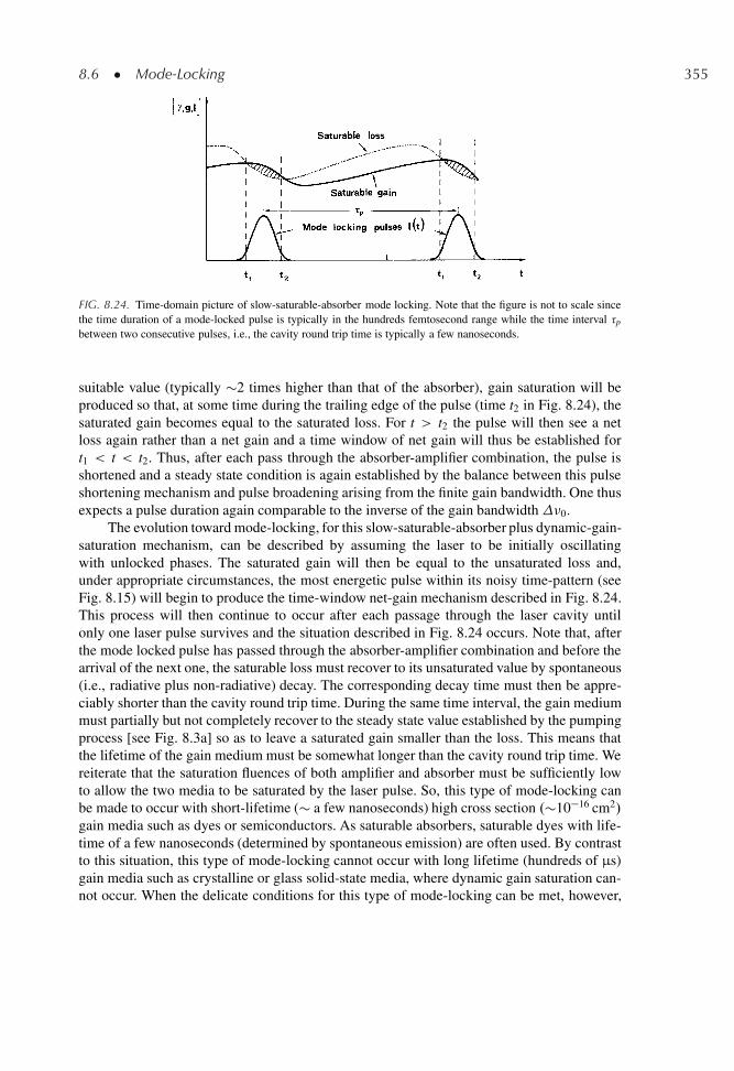
8.6 � Mode-Locking 355
FIG. 8.24. Time-domain picture of slow-saturable-absorber mode locking. Note that the figure is not to scale sincethe time duration of a mode-locked pulse is typically in the hundreds femtosecond range while the time interval �p
between two consecutive pulses, i.e., the cavity round trip time is typically a few nanoseconds.
suitable value (typically �2 times higher than that of the absorber), gain saturation will beproduced so that, at some time during the trailing edge of the pulse (time t2 in Fig. 8.24), thesaturated gain becomes equal to the saturated loss. For t > t2 the pulse will then see a netloss again rather than a net gain and a time window of net gain will thus be established fort1 < t < t2. Thus, after each pass through the absorber-amplifier combination, the pulse isshortened and a steady state condition is again established by the balance between this pulseshortening mechanism and pulse broadening arising from the finite gain bandwidth. One thusexpects a pulse duration again comparable to the inverse of the gain bandwidth�0.
The evolution toward mode-locking, for this slow-saturable-absorber plus dynamic-gain-saturation mechanism, can be described by assuming the laser to be initially oscillatingwith unlocked phases. The saturated gain will then be equal to the unsaturated loss and,under appropriate circumstances, the most energetic pulse within its noisy time-pattern (seeFig. 8.15) will begin to produce the time-window net-gain mechanism described in Fig. 8.24.This process will then continue to occur after each passage through the laser cavity untilonly one laser pulse survives and the situation described in Fig. 8.24 occurs. Note that, afterthe mode locked pulse has passed through the absorber-amplifier combination and before thearrival of the next one, the saturable loss must recover to its unsaturated value by spontaneous(i.e., radiative plus non-radiative) decay. The corresponding decay time must then be appre-ciably shorter than the cavity round trip time. During the same time interval, the gain mediummust partially but not completely recover to the steady state value established by the pumpingprocess [see Fig. 8.3a] so as to leave a saturated gain smaller than the loss. This means thatthe lifetime of the gain medium must be somewhat longer than the cavity round trip time. Wereiterate that the saturation fluences of both amplifier and absorber must be sufficiently lowto allow the two media to be saturated by the laser pulse. So, this type of mode-locking canbe made to occur with short-lifetime (� a few nanoseconds) high cross section .�10�16 cm2/
gain media such as dyes or semiconductors. As saturable absorbers, saturable dyes with life-time of a few nanoseconds (determined by spontaneous emission) are often used. By contrastto this situation, this type of mode-locking cannot occur with long lifetime (hundreds of μs)gain media such as crystalline or glass solid-state media, where dynamic gain saturation can-not occur. When the delicate conditions for this type of mode-locking can be met, however,
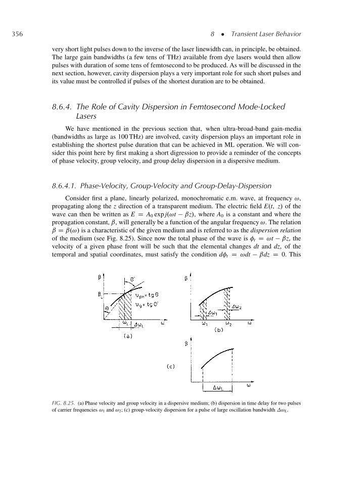
356 8 � Transient Laser Behavior
very short light pulses down to the inverse of the laser linewidth can, in principle, be obtained.The large gain bandwidths (a few tens of THz) available from dye lasers would then allowpulses with duration of some tens of femtosecond to be produced. As will be discussed in thenext section, however, cavity dispersion plays a very important role for such short pulses andits value must be controlled if pulses of the shortest duration are to be obtained.
8.6.4. The Role of Cavity Dispersion in Femtosecond Mode-LockedLasers
We have mentioned in the previous section that, when ultra-broad-band gain-media(bandwidths as large as 100 THz) are involved, cavity dispersion plays an important role inestablishing the shortest pulse duration that can be achieved in ML operation. We will con-sider this point here by first making a short digression to provide a reminder of the conceptsof phase velocity, group velocity, and group delay dispersion in a dispersive medium.
8.6.4.1. Phase-Velocity, Group-Velocity and Group-Delay-Dispersion
Consider first a plane, linearly polarized, monochromatic e.m. wave, at frequency !,propagating along the z direction of a transparent medium. The electric field E.t, z/ of thewave can then be written as E D A0 exp j.!t � ˇz/, where A0 is a constant and where thepropagation constant, ˇ, will generally be a function of the angular frequency!. The relationˇ D ˇ.!/ is a characteristic of the given medium and is referred to as the dispersion relationof the medium (see Fig. 8.25). Since now the total phase of the wave is �t D !t � ˇz, thevelocity of a given phase front will be such that the elemental changes dt and dz, of thetemporal and spatial coordinates, must satisfy the condition d�t D !dt � ˇdz D 0. This
FIG. 8.25. (a) Phase velocity and group velocity in a dispersive medium; (b) dispersion in time delay for two pulsesof carrier frequencies !1 and !2; (c) group-velocity dispersion for a pulse of large oscillation bandwidth !L.
8.6 � Mode-Locking 357
shows that the phase front moves at a velocity
�ph D dz
dtD !
ˇ(8.6.24)
referred to as the phase velocity of the wave.Consider next a light pulse traveling in the medium and let !L and!L be, respectively,
the center frequency and the width of the corresponding spectrum (Fig. 8.25a). Assume alsothat the dispersion relation, over the bandwidth!L, can be approximated by a linear relation,viz. ˇ D ˇL C.dˇ=d!/!D!L .!�!L/, where ˇL is the propagation constant corresponding tothe frequency !L. In this case, upon considering a Fourier expansion of wave, one can showthat the electric field of the wave can be expressed as (see Appendix G)
E.t, z/ D AŒt � .z=�g/� expŒj.!Lt � ˇLz/� (8.6.25)
where A is the pulse amplitude, expŒj.!Lt � ˇLz/� is the carrier wave, and �g is given by
�g D�
d!
dˇ
�ˇDˇL
(8.6.26)
The fact that the pulse amplitude is a function of the variable t � .z=�g/ means that thepulse propagates without changing its shape and at a speed �g. This velocity is referred to asthe group velocity of the pulse and, according to Eq. (8.6.26), is given by the slope of the ! vsˇ relation at ! D !L (i.e. �g D tg 0, see Fig. 8.25a). Note also that, for a general dispersionrelation such as that of Fig. 8.25a, the phase velocity of the carrier wave (�ph D tg , seeFig. 8.25a) will be different from the group velocity.
According to the previous considerations, the pulse, after traversing the length l of themedium, will be subjected to a time delay
�g D l
�gD l
�dˇ
d!
�!L
D �0.!L/ (8.6.27)
For the previous equation, we have defined a phase �, dependent on the frequency !,such that
�.! � !L/ D ˇ.! � !L/l (8.6.28)
and we have called �0.!L/ D Œd�.! � !L/=d!�!L . For obvious reasons, the quantity �g D�0.!L/ is referred to as the group delay of the medium at frequency !L.
Let us now see what happens when two pulses, with bandwidths!1 and !2 centeredat !1 and !2, respectively, are traveling in the medium (!2 > !1, see Fig. 8.25b). If theslope of the dispersion relation is different at the two frequencies, the two pulses will travel atdifferent group velocities �g1 and �g2 . Thus, if the peaks of the two pulses enter the mediumat the same time, then, after traversing the length l of the medium, they will become separatedin time by a delay
�g D �0.!2/� �0.!1/ Š �00.!1/ � .!2 � !1/ (8.6.29)
358 8 � Transient Laser Behavior
where we have used the symbol �00.!1/ D Œd2�=d!2�!1 . Note that the last equation holdsexactly if the relation between � and !, in the frequency range between !1 and !2, can beapproximated by a parabolic law viz.
� D �L C�
d�
d!
�!L
.! � !L/C 1
2
�d2�
d!2
�!L
.! � !L/2 (8.6.30)
Consider next the case of a light pulse with a bandwidth!L so large that it is no longera good approximation to describe the dispersion relation by a linear law (Fig. 8.25c). In thiscase, different spectral regions of the pulse will travel with different group velocities and,consequently, the pulse will broaden as it propagates. Again assuming that the dispersion rela-tion, within the bandwidth !L, can be approximated by a parabolic law, then, according toEq. (8.6.29), the broadening of the pulse due to dispersion,�d, will be given approximatelyby the difference in group delay between the fastest spectral component and the slowest one.According to Eq. (8.6.29) we then have
�d Š j�00.!L/j !L (8.6.31)
The quantity �00.!L/ is referred to as the group delay dispersion (GDD) of the mediumat frequency !L. Its magnitude gives the pulse broadening per unit bandwidth of the pulse.From Eqs. (8.6.28) and (8.6.31) one then sees that �d can also be written as
�d Š l
ˇˇ� d2ˇ
d!2
�!L
ˇˇ !L (8.6.32)
The quantity, GVD, expressed by
GVD D .d2ˇ = d2!/!L D Œd.1=�g/ = d!�!L (8.6.33)
is usually referred to as the group velocity dispersion at frequency !L. Its magnitude gives thepulse broadening per unit length of the medium and per unit bandwidth of the pulse. It shouldbe observed that the concept of group velocity dispersion is straightforward, in application,only for a homogeneous medium. For an inhomogeneous or multi-component medium, suchas the two prism pairs of Fig. 8.26 or a multilayer dielectric mirror, the concept of group delaydispersion is more easy to consider.
8.6.4.2. Limitation on Pulse Duration due to Group-Delay Dispersion
When a dispersive medium is present within a ML laser cavity, an approximated valueof the steady state pulse duration can be obtained from the condition that the relative timeshortening, .ı�p=�p/s, due to the net gain time window (see Fig. 8.22 or 8.24), must equalthe pulse broadening due to both the gain medium, .ı�p=�p/g, and the dispersive medium,.ı�p=�p/D. For the sake of simplicity, we will consider here a ring cavity in which the pulseis sequentially passing through the gain medium, the dispersive medium, and through what-ever element provides the self-amplitude-modulation (e.g., a fast saturable absorber). We will
8.6 � Mode-Locking 359
assume that the light pulse has a Gaussian intensity profile with pulsewidth (FWHM)�p, andthat the dispersive medium can be described, at a general frequency!, by its group-delay dis-persion �00 D �00.!/. The gain medium is assumed to be homogeneously broadened and willbe described by its saturated single pass gain, g0 D N0� l, and its linewidth (FWHM) !0.
For small changes of pulse duration, the relative pulse broadenings, .ı�p=�p/g and.ı�p=�p/D, after passing through the gain medium and the dispersive medium, are shownin Appendix G to be given, respectively, by
�ı�p
�p
�g
D�
2 ln 2
2
� 1
�2p�
20
!g0 (8.6.34)
where �0 D !0=2 , and by�ı�p
�p
�D
D .8 ln2 2/�002
�4p
(8.6.35)
where �00 is calculated at the central frequency, !L, of the laser pulse.The steady state pulse duration can now be obtained from the condition that the relative
time shortening, .ı�p=�p/s, due to the net gain time window must be equal to the pulse broad-ening due to both the gain medium and the dispersive medium. From Eqs. (8.6.34) and (8.6.35)we then get
�ı�p
�p
�s
D 0.14g0
�2p�
20
C 3.84�002
�4p
(8.6.36)
Note that the two terms on the right hand side of Eq. (8.6.36) are inversely proportional to�2
p and �4p , respectively. This means that the importance of GDD in establishing the pulse
duration becomes more important as �p decreases. To get an estimate of the pulse-width atwhich GDD begins to become important we equate the two terms on the right hand side ofEq. (8.6.36). We get
�p D�
27.4
g0
� 1=2 ˇ�00ˇ �0 (8.6.37)
Assuming, as an example, �0 Š 100 THz (as appropriate for a Ti:sapphire gainmedium) and �00 D 100 fs2 (equivalent, at � Š 800 nm, to the presence of �2 mm ofquartz material in the cavity) and g0 D 0.1, we get from (8.6.37) �p Š 162 fs. This meansthat, to get pulses shorter than �150 fs, down to perhaps the inverse of the gain linewidth�0 .�
0p D 1=�0 Š 4 fs/, one needs to reduce GDD by about an order of magnitude.
To obtain the shortest pulses, when second order dispersion, GDD, is suitably compen-sated, one also needs to compensate higher order dispersion terms in the power expansionEq. (8.6.30). Of course, the next term to be considered would be third order dispersion, TOD,defined as TOD D �000 D ˇ000 l, where the third derivatives are taken at the laser’s centerfrequency, !L. We shall not consider, at any length, the effects produced by TOD on an inci-dent pulse, and, for a discussion of this topic, we refer to the literature..24/ We will just pointout that, in the case of e.g., a Ti:sapphire laser .�0 Š 100 THz/, TOD begins to play apulse-limiting role for pulses shorter than �30 fs.
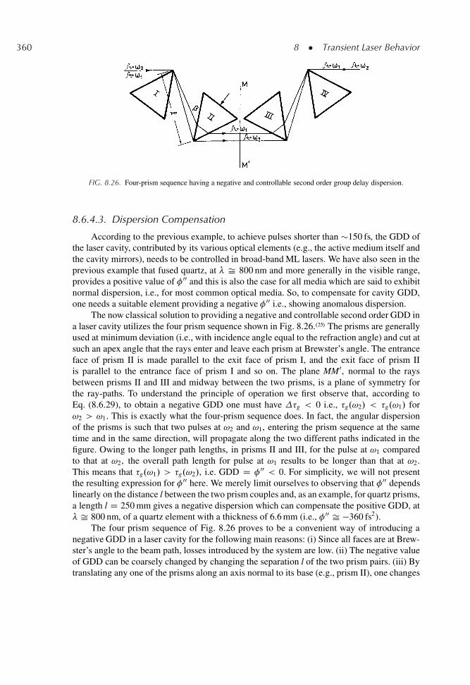
360 8 � Transient Laser Behavior
FIG. 8.26. Four-prism sequence having a negative and controllable second order group delay dispersion.
8.6.4.3. Dispersion Compensation
According to the previous example, to achieve pulses shorter than �150 fs, the GDD ofthe laser cavity, contributed by its various optical elements (e.g., the active medium itself andthe cavity mirrors), needs to be controlled in broad-band ML lasers. We have also seen in theprevious example that fused quartz, at � Š 800 nm and more generally in the visible range,provides a positive value of �00 and this is also the case for all media which are said to exhibitnormal dispersion, i.e., for most common optical media. So, to compensate for cavity GDD,one needs a suitable element providing a negative �00 i.e., showing anomalous dispersion.
The now classical solution to providing a negative and controllable second order GDD ina laser cavity utilizes the four prism sequence shown in Fig. 8.26..25/ The prisms are generallyused at minimum deviation (i.e., with incidence angle equal to the refraction angle) and cut atsuch an apex angle that the rays enter and leave each prism at Brewster’s angle. The entranceface of prism II is made parallel to the exit face of prism I, and the exit face of prism IIis parallel to the entrance face of prism I and so on. The plane MM0, normal to the raysbetween prisms II and III and midway between the two prisms, is a plane of symmetry forthe ray-paths. To understand the principle of operation we first observe that, according toEq. (8.6.29), to obtain a negative GDD one must have �g < 0 i.e., �g.!2/ < �g.!1/ for!2 > !1. This is exactly what the four-prism sequence does. In fact, the angular dispersionof the prisms is such that two pulses at !2 and !1, entering the prism sequence at the sametime and in the same direction, will propagate along the two different paths indicated in thefigure. Owing to the longer path lengths, in prisms II and III, for the pulse at !1 comparedto that at !2, the overall path length for pulse at !1 results to be longer than that at !2.This means that �g.!1/ > �g.!2/, i.e. GDD D �00 < 0. For simplicity, we will not presentthe resulting expression for �00 here. We merely limit ourselves to observing that �00 dependslinearly on the distance l between the two prism couples and, as an example, for quartz prisms,a length l D 250 mm gives a negative dispersion which can compensate the positive GDD, at� Š 800 nm, of a quartz element with a thickness of 6.6 mm (i.e., �00 Š �360 fs2).
The four prism sequence of Fig. 8.26 proves to be a convenient way of introducing anegative GDD in a laser cavity for the following main reasons: (i) Since all faces are at Brew-ster’s angle to the beam path, losses introduced by the system are low. (ii) The negative valueof GDD can be coarsely changed by changing the separation l of the two prism pairs. (iii) Bytranslating any one of the prisms along an axis normal to its base (e.g., prism II), one changes
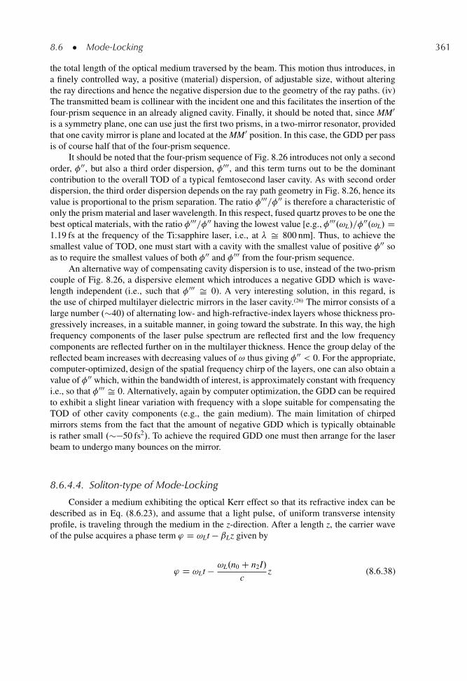
8.6 � Mode-Locking 361
the total length of the optical medium traversed by the beam. This motion thus introduces, ina finely controlled way, a positive (material) dispersion, of adjustable size, without alteringthe ray directions and hence the negative dispersion due to the geometry of the ray paths. (iv)The transmitted beam is collinear with the incident one and this facilitates the insertion of thefour-prism sequence in an already aligned cavity. Finally, it should be noted that, since MM0is a symmetry plane, one can use just the first two prisms, in a two-mirror resonator, providedthat one cavity mirror is plane and located at the MM0 position. In this case, the GDD per passis of course half that of the four-prism sequence.
It should be noted that the four-prism sequence of Fig. 8.26 introduces not only a secondorder, �00, but also a third order dispersion, �000, and this term turns out to be the dominantcontribution to the overall TOD of a typical femtosecond laser cavity. As with second orderdispersion, the third order dispersion depends on the ray path geometry in Fig. 8.26, hence itsvalue is proportional to the prism separation. The ratio �000=�00 is therefore a characteristic ofonly the prism material and laser wavelength. In this respect, fused quartz proves to be one thebest optical materials, with the ratio �000=�00 having the lowest value [e.g., �000.!L/=�
00.!L/ D1.19 fs at the frequency of the Ti:sapphire laser, i.e., at � Š 800 nm]. Thus, to achieve thesmallest value of TOD, one must start with a cavity with the smallest value of positive �00 soas to require the smallest values of both �00 and �000 from the four-prism sequence.
An alternative way of compensating cavity dispersion is to use, instead of the two-prismcouple of Fig. 8.26, a dispersive element which introduces a negative GDD which is wave-length independent (i.e., such that �000 Š 0). A very interesting solution, in this regard, isthe use of chirped multilayer dielectric mirrors in the laser cavity..26/ The mirror consists of alarge number .�40/ of alternating low- and high-refractive-index layers whose thickness pro-gressively increases, in a suitable manner, in going toward the substrate. In this way, the highfrequency components of the laser pulse spectrum are reflected first and the low frequencycomponents are reflected further on in the multilayer thickness. Hence the group delay of thereflected beam increases with decreasing values of ! thus giving �00 < 0. For the appropriate,computer-optimized, design of the spatial frequency chirp of the layers, one can also obtain avalue of �00 which, within the bandwidth of interest, is approximately constant with frequencyi.e., so that �000 Š 0. Alternatively, again by computer optimization, the GDD can be requiredto exhibit a slight linear variation with frequency with a slope suitable for compensating theTOD of other cavity components (e.g., the gain medium). The main limitation of chirpedmirrors stems from the fact that the amount of negative GDD which is typically obtainableis rather small .��50 fs2/. To achieve the required GDD one must then arrange for the laserbeam to undergo many bounces on the mirror.
8.6.4.4. Soliton-type of Mode-Locking
Consider a medium exhibiting the optical Kerr effect so that its refractive index can bedescribed as in Eq. (8.6.23), and assume that a light pulse, of uniform transverse intensityprofile, is traveling through the medium in the z-direction. After a length z, the carrier waveof the pulse acquires a phase term ' D !Lt � ˇLz given by
' D !Lt � !L.n0 C n2I/
cz (8.6.38)
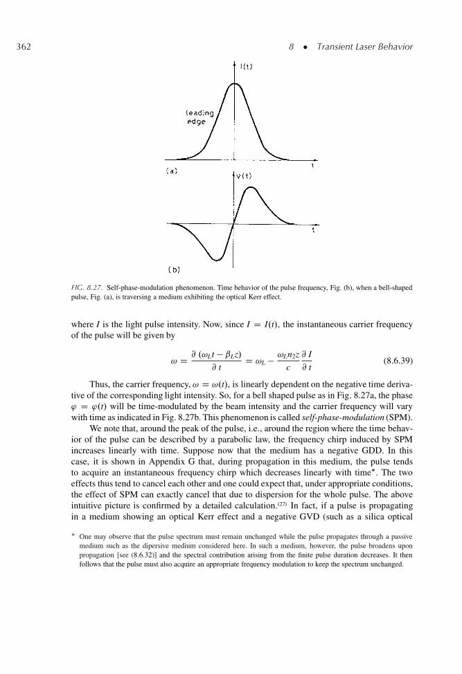
362 8 � Transient Laser Behavior
FIG. 8.27. Self-phase-modulation phenomenon. Time behavior of the pulse frequency, Fig. (b), when a bell-shapedpulse, Fig. (a), is traversing a medium exhibiting the optical Kerr effect.
where I is the light pulse intensity. Now, since I D I.t/, the instantaneous carrier frequencyof the pulse will be given by
! D @ .!Lt � ˇLz/
@ tD !L � !Ln2z
c
@ I
@ t(8.6.39)
Thus, the carrier frequency,! D !.t/, is linearly dependent on the negative time deriva-tive of the corresponding light intensity. So, for a bell shaped pulse as in Fig. 8.27a, the phase' D '.t/ will be time-modulated by the beam intensity and the carrier frequency will varywith time as indicated in Fig. 8.27b. This phenomenon is called self-phase-modulation (SPM).
We note that, around the peak of the pulse, i.e., around the region where the time behav-ior of the pulse can be described by a parabolic law, the frequency chirp induced by SPMincreases linearly with time. Suppose now that the medium has a negative GDD. In thiscase, it is shown in Appendix G that, during propagation in this medium, the pulse tendsto acquire an instantaneous frequency chirp which decreases linearly with time�. The twoeffects thus tend to cancel each other and one could expect that, under appropriate conditions,the effect of SPM can exactly cancel that due to dispersion for the whole pulse. The aboveintuitive picture is confirmed by a detailed calculation..27/ In fact, if a pulse is propagatingin a medium showing an optical Kerr effect and a negative GVD (such as a silica optical
� One may observe that the pulse spectrum must remain unchanged while the pulse propagates through a passivemedium such as the dipersive medium considered here. In such a medium, however, the pulse broadens uponpropagation [see (8.6.32)] and the spectral contribution arising from the finite pulse duration decreases. It thenfollows that the pulse must also acquire an appropriate frequency modulation to keep the spectrum unchanged.
8.6 � Mode-Locking 363
fiber at � > 1300 nm), the pulse propagation, due to the presence of SPM, is described bya nonlinear wave equation which admits pulsed solutions that propagate without distortion.The time behavior of the corresponding electric field, for the lowest order solution, turns outto be described by a hyperbolic secant function [i.e., A.t0/ / sech .t0=�p/], i.e., the pulse isunchirped and the whole pulse propagates without distortion as a result of the mutual compen-sation of SPM and GVD, as discussed above. These solutions are called solitary solutions ofthe nonlinear wave equation or solitons. One of the most interesting properties of the lowestorder soliton is that its pulsewidth�p (FWHM) is related to the pulse peak power, Pp, by theequation.27/
�2p D 3.11jb2j
� Pp(8.6.40)
where b2 D .d2ˇ=d!2/!L , � D n2!L=cAeff , and Aeff is the effective area of the beam (Aeff D w2 for a Gaussian beam of spot size w). One can also show that �=2 is simply the nonlinearphase shift per unit length per unit peak power [see also Eq. (8.6.38)].
One can now ask the question as to whether solitary pulses can be produced in a MLlaser cavity containing a medium exhibiting the optical Kerr effect and with overall negativeGDD. The answer to this question is that solitary solutions, alone, are unstable in a MLlaser cavity.28/ but can become stabilized by some nonlinear loss mechanism producing aself amplitude modulation (see Fig. 8.22 or Fig. 8.24). In this case, if one neglects pulsebroadening arising from the finite gain bandwidth and higher order dispersion, one gets anapproximate steady-state solution that is equivalent to the fundamental soliton propagation inoptical fibers with anomalous dispersion. In particular, according to Eq. (8.6.40), the pulseduration turns out to be proportional to the inverse of the pulse energy E .E Š 2.27 Pp�p/
according to the relation.29/
�p D 3.53j�00jı E
(8.6.41)
where �00 is the GDD for the round trip in the laser cavity and ı is the nonlinear round-tripphase shift per unit power in the Kerr medium and thus given by ı D � lK , where lK is thelength of the Kerr medium. From Eq. (8.6.41), taking �00 D �200 fs2, ı � 10�6 W�1, andE � 50 nJ (as appropriate for a ML Ti:sapphire laser) one obtains �p Š 14 fs. Indeed, soli-tary solutions have been observed in both ML Ti:sapphire and ML dye lasers by carefullyadjusting the laser parameters..29,30/ In both these cases, ML was exploiting a mechanism ofself amplitude modulation, such as that occurring by KLM or by a slow saturable absorbercombined with dynamic gain saturation. In both cases, very short (10–20 fs) pulses can begenerated either by the soliton mechanism alone or by the combined action of pulse broaden-ing due to the finite gain bandwidth. It is also important to note that very short ML light pulses.�100 fs/ have been produced by this soliton-type mechanism even using ML elements pro-viding a much slower time window of net gain (e.g., semiconductor saturable absorbers withpicosecond relaxation time)..31/ In this case, the ML element just helps to stabilizing the soli-ton solution while the pulse duration is essentially determined by the soliton equation givenby Eq. (8.6.41).
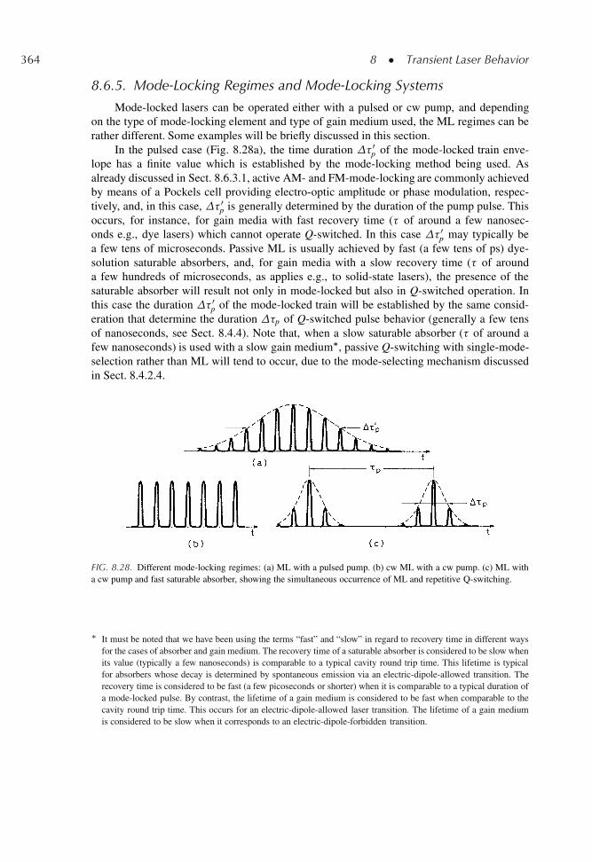
364 8 � Transient Laser Behavior
8.6.5. Mode-Locking Regimes and Mode-Locking Systems
Mode-locked lasers can be operated either with a pulsed or cw pump, and dependingon the type of mode-locking element and type of gain medium used, the ML regimes can berather different. Some examples will be briefly discussed in this section.
In the pulsed case (Fig. 8.28a), the time duration � 0p of the mode-locked train enve-
lope has a finite value which is established by the mode-locking method being used. Asalready discussed in Sect. 8.6.3.1, active AM- and FM-mode-locking are commonly achievedby means of a Pockels cell providing electro-optic amplitude or phase modulation, respec-tively, and, in this case, � 0
p is generally determined by the duration of the pump pulse. Thisoccurs, for instance, for gain media with fast recovery time (� of around a few nanosec-onds e.g., dye lasers) which cannot operate Q-switched. In this case � 0
p may typically bea few tens of microseconds. Passive ML is usually achieved by fast (a few tens of ps) dye-solution saturable absorbers, and, for gain media with a slow recovery time (� of arounda few hundreds of microseconds, as applies e.g., to solid-state lasers), the presence of thesaturable absorber will result not only in mode-locked but also in Q-switched operation. Inthis case the duration � 0
p of the mode-locked train will be established by the same consid-eration that determine the duration �p of Q-switched pulse behavior (generally a few tensof nanoseconds, see Sect. 8.4.4). Note that, when a slow saturable absorber (� of around afew nanoseconds) is used with a slow gain medium�, passive Q-switching with single-mode-selection rather than ML will tend to occur, due to the mode-selecting mechanism discussedin Sect. 8.4.2.4.
FIG. 8.28. Different mode-locking regimes: (a) ML with a pulsed pump. (b) cw ML with a cw pump. (c) ML witha cw pump and fast saturable absorber, showing the simultaneous occurrence of ML and repetitive Q-switching.
� It must be noted that we have been using the terms “fast” and “slow” in regard to recovery time in different waysfor the cases of absorber and gain medium. The recovery time of a saturable absorber is considered to be slow whenits value (typically a few nanoseconds) is comparable to a typical cavity round trip time. This lifetime is typicalfor absorbers whose decay is determined by spontaneous emission via an electric-dipole-allowed transition. Therecovery time is considered to be fast (a few picoseconds or shorter) when it is comparable to a typical duration ofa mode-locked pulse. By contrast, the lifetime of a gain medium is considered to be fast when comparable to thecavity round trip time. This occurs for an electric-dipole-allowed laser transition. The lifetime of a gain mediumis considered to be slow when it corresponds to an electric-dipole-forbidden transition.
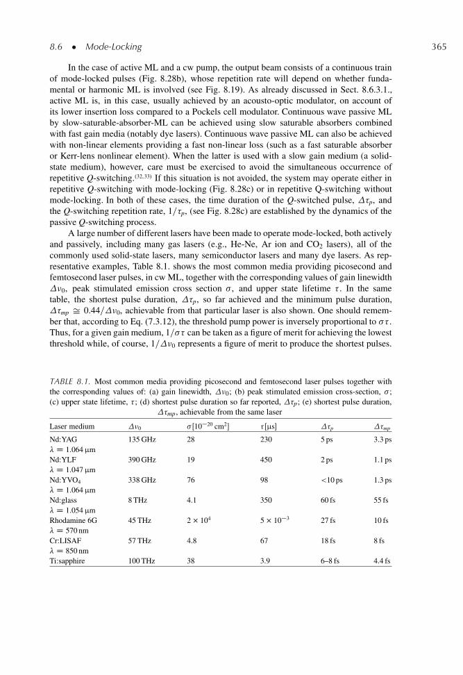
8.6 � Mode-Locking 365
In the case of active ML and a cw pump, the output beam consists of a continuous trainof mode-locked pulses (Fig. 8.28b), whose repetition rate will depend on whether funda-mental or harmonic ML is involved (see Fig. 8.19). As already discussed in Sect. 8.6.3.1.,active ML is, in this case, usually achieved by an acousto-optic modulator, on account ofits lower insertion loss compared to a Pockels cell modulator. Continuous wave passive MLby slow-saturable-absorber-ML can be achieved using slow saturable absorbers combinedwith fast gain media (notably dye lasers). Continuous wave passive ML can also be achievedwith non-linear elements providing a fast non-linear loss (such as a fast saturable absorberor Kerr-lens nonlinear element). When the latter is used with a slow gain medium (a solid-state medium), however, care must be exercised to avoid the simultaneous occurrence ofrepetitive Q-switching..32,33/ If this situation is not avoided, the system may operate either inrepetitive Q-switching with mode-locking (Fig. 8.28c) or in repetitive Q-switching withoutmode-locking. In both of these cases, the time duration of the Q-switched pulse, �p, andthe Q-switching repetition rate, 1=�p, (see Fig. 8.28c) are established by the dynamics of thepassive Q-switching process.
A large number of different lasers have been made to operate mode-locked, both activelyand passively, including many gas lasers (e.g., He-Ne, Ar ion and CO2 lasers), all of thecommonly used solid-state lasers, many semiconductor lasers and many dye lasers. As rep-resentative examples, Table 8.1. shows the most common media providing picosecond andfemtosecond laser pulses, in cw ML, together with the corresponding values of gain linewidth�0, peak stimulated emission cross section � , and upper state lifetime � . In the sametable, the shortest pulse duration, �p, so far achieved and the minimum pulse duration,�mp Š 0.44=�0, achievable from that particular laser is also shown. One should remem-ber that, according to Eq. (7.3.12), the threshold pump power is inversely proportional to �� .Thus, for a given gain medium, 1=�� can be taken as a figure of merit for achieving the lowestthreshold while, of course, 1=�0 represents a figure of merit to produce the shortest pulses.
TABLE 8.1. Most common media providing picosecond and femtosecond laser pulses together withthe corresponding values of: (a) gain linewidth, �0; (b) peak stimulated emission cross-section, � ;(c) upper state lifetime, � ; (d) shortest pulse duration so far reported, �p; (e) shortest pulse duration,
�mp, achievable from the same laser
Laser medium �0 �Œ10�20 cm2� � Œμs� �p �mp
Nd:YAG 135 GHz 28 230 5 ps 3.3 ps� D 1.064 μmNd:YLF 390 GHz 19 450 2 ps 1.1 ps� D 1.047 μmNd:YVO4 338 GHz 76 98 <10 ps 1.3 ps� D 1.064 μmNd:glass 8 THz 4.1 350 60 fs 55 fs� D 1.054 μmRhodamine 6G 45 THz 2 104 5 10�3 27 fs 10 fs� D 570 nmCr:LISAF 57 THz 4.8 67 18 fs 8 fs� D 850 nmTi:sapphire 100 THz 38 3.9 6–8 fs 4.4 fs
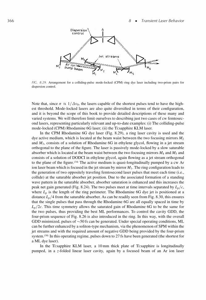
366 8 � Transient Laser Behavior
FIG. 8.29. Arrangement for a colliding-pulse mode-locked (CPM) ring dye laser including two-prism pairs fordispersion control.
Note that, since � / 1=�0, the lasers capable of the shortest pulses tend to have the high-est threshold. Mode-locked lasers are also quite diversified in terms of their configuration,and it is beyond the scope of this book to provide detailed descriptions of these many andvaried systems. We will therefore limit ourselves to describing just two cases of cw femtosec-ond lasers, representing particularly relevant and up-to-date examples: (i) The colliding-pulsemode-locked (CPM) Rhodamine 6G laser; (ii) the Ti:sapphire KLM laser.
In the CPM Rhodamine 6G dye laser (Fig. 8.29), a ring laser cavity is used and thedye active medium, which is located at the beam waist between the two focusing mirrors M2
and M3, consists of a solution of Rhodamine 6G in ethylene glycol, flowing in a jet streamorthogonal to the plane of the figure. The laser is passively mode-locked by a slow saturableabsorber which is located at the beam waist between the two focusing mirrors M4 and M5 andconsists of a solution of DODCI in ethylene glycol, again flowing as a jet stream orthogonalto the plane of the figure..34/ The active medium is quasi-longitudinally pumped by a cw Arion laser beam which is focused in the jet stream by mirror M1. The ring configuration leads tothe generation of two oppositely traveling femtosecond laser pulses that meet each time (i.e.,collide) at the saturable absorber jet position. Due to the associated formation of a standingwave pattern in the saturable absorber, absorber saturation is enhanced and this increases thepeak net gain generated (Fig. 8.24). The two pulses meet at time intervals separated by Lp=c,where Lp is the length of the ring perimeter. The Rhodamine 6G dye jet is positioned at adistance Lp=4 from the saturable absorber. As can be readily seen from Fig. 8.30, this ensuresthat the single pulses that pass through the Rhodamine 6G are all equally spaced in time byLp=2c. This time symmetry allows the saturated gain of Rhodamine 6G to be the same forthe two pulses, thus providing the best ML performances. To control the cavity GDD, thefour-prism sequence of Fig. 8.26 is also introduced in the ring. In this way, with the overallGDD minimized, pulses of �50 fs can be generated. Under special operating conditions, MLcan be further enhanced by a soliton-type mechanism, via the phenomenon of SPM within thejet streams and with the required amount of negative GDD being provided by the four-prismsystem..30/ In this operating regime, pulses down to 27 fs have been generated (the shortest fora ML dye laser).
In the Ti:sapphire KLM laser, a 10 mm thick plate of Ti:sapphire is longitudinallypumped, in a z-folded linear laser cavity, again by a focused beam of an Ar ion laser
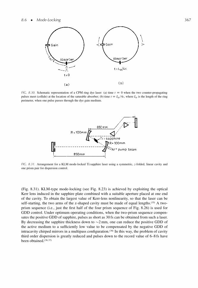
8.6 � Mode-Locking 367
FIG. 8.30. Schematic representation of a CPM ring dye laser: (a) time t D 0 when the two counter-propagatingpulses meet (collide) at the location of the saturable absorber; (b) time t D Lp=4c, where Lp is the length of the ringperimeter, when one pulse passes through the dye gain medium.
FIG. 8.31. Arrangement for a KLM mode-locked Ti:sapphire laser using a symmetric, z-folded, linear cavity andone prism pair for dispersion control.
(Fig. 8.31). KLM-type mode-locking (see Fig. 8.23) is achieved by exploiting the opticalKerr lens induced in the sapphire plate combined with a suitable aperture placed at one endof the cavity. To obtain the largest value of Kerr-lens nonlinearity, so that the laser can beself-starting, the two arms of the z-shaped cavity must be made of equal lengths..35/ A two-prism sequence (i.e., just the first half of the four prism sequence of Fig. 8.26) is used forGDD control. Under optimum operating conditions, when the two-prism sequence compen-sates the positive GDD of sapphire, pulses as short as 30 fs can be obtained from such a laser.By decreasing the sapphire thickness down to �2 mm, one can reduce the positive GDD ofthe active medium to a sufficiently low value to be compensated by the negative GDD ofintracavity chirped mirrors in a multipass configuration..36/ In this way, the problem of cavitythird order dispersion is greatly reduced and pulses down to the record value of 6–8 fs havebeen obtained..36,37/
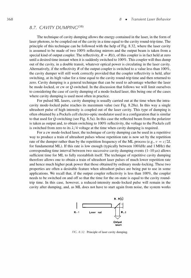
368 8 � Transient Laser Behavior
8.7. CAVITY DUMPING.38/
The technique of cavity dumping allows the energy contained in the laser, in the form oflaser photons, to be coupled out of the cavity in a time equal to the cavity round-trip time. Theprinciple of this technique can be followed with the help of Fig. 8.32, where the laser cavityis assumed to be made of two 100% reflecting mirrors and the output beam is taken from aspecial kind of output coupler. The reflectivity, R D R.t/, of this coupler is in fact held at zerountil a desired time instant when it is suddenly switched to 100%. This coupler will thus dumpout of the cavity, in a double transit, whatever optical power is circulating in the laser cavity.Alternatively, if the reflectivity R of the output coupler is switched to a value less than 100%,the cavity dumper will still work correctly provided that the coupler reflectivity is held, afterswitching, at its high value for a time equal to the cavity round-trip time and then returned tozero. Cavity dumping is a general technique that can be used to advantage whether the laserbe mode-locked, or cw or Q-switched. In the discussion that follows we will limit ourselvesto considering the case of cavity dumping of a mode-locked laser, this being one of the caseswhere cavity dumping is used most often in practice.
For pulsed ML lasers, cavity dumping is usually carried out at the time when the intra-cavity mode-locked pulse reaches its maximum value (see Fig. 8.28a). In this way a singleultrashort pulse of high intensity is coupled out of the laser cavity. This type of dumping isoften obtained by a Pockels cell electro-optic modulator used in a configuration that is similarto that used for Q-switching (see Fig. 8.5a). In this case the reflected beam from the polarizeris taken as output and, to obtain switching to 100% reflectivity, the voltage to the Pockels cellis switched from zero to its �=4 voltage at the time when cavity dumping is required.
For a cw mode-locked laser, the technique of cavity dumping can be used in a repetitiveway to produce a train of ultrashort pulses whose repetition rate is now set by the repetitionrate of the dumper rather than by the repetition frequency of the ML process (e.g., � D c=2Lfor fundamental ML). If this rate is low enough (typically between 100 kHz and 1 MHz) thecorresponding time interval between two successive cavity dumping events .1–10 μs/ allowssufficient time for ML to fully reestablish itself. The technique of repetitive cavity dumpingtherefore allows one to obtain a train of ultrashort laser pulses of much lower repetition rateand hence much higher peak power that those obtained by ordinary mode-locking. These twoproperties are often a desirable feature when ultrashort pulses are being put to use in someapplications. We recall that, if the output coupler reflectivity is less than 100%, the couplerneeds to be switched on and off so that the time for the on-state is equal to the cavity round-trip time. In this case, however, a reduced-intensity mode-locked pulse will remain in thecavity after dumping, and, as ML does not have to start again from noise, the system works
FIG. 8.32. Principle of laser cavity dumping.
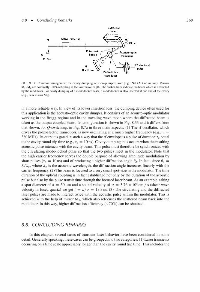
8.8 � Concluding Remarks 369
FIG. 8.33. Common arrangement for cavity dumping of a cw-pumped laser (e.g., Nd:YAG or Ar ion). MirrorsM1–M3 are nominally 100% reflecting at the laser wavelength. The broken lines indicate the beam which is diffractedby the modulator. For cavity dumping of a mode-locked laser, a mode-locker is also inserted at one end of the cavity(e.g., near mirror M1).
in a more reliable way. In view of its lower insertion loss, the dumping device often used forthis application is the acousto-optic cavity dumper. It consists of an acousto-optic modulatorworking in the Bragg regime and in the traveling-wave mode where the diffracted beam istaken as the output coupled beam. Its configuration is shown in Fig. 8.33 and it differs fromthat shown, for Q-switching, in Fig. 8.7a in three main aspects: (1) The rf oscillator, whichdrives the piezoelectric transducer, is now oscillating at a much higher frequency (e.g., � D380 MHz). Its output is gated in such a way that the rf envelope is a pulse of duration �p equalto the cavity round trip time (e.g., �p D 10 ns). Cavity dumping thus occurs when the resultingacoustic pulse interacts with the cavity beam. This pulse must therefore be synchronized withthe circulating mode-locked pulse so that the two pulses meet in the modulator. Note thatthe high carrier frequency serves the double purpose of allowing amplitude modulation byshort pulses .�p D 10 ns/ and of producing a higher diffraction angle d. In fact, since d D�=�a, where �a is the acoustic wavelength, the diffraction angle increases linearly with thecarrier frequency. (2) The beam is focused to a very small spot-size in the modulator. The timeduration of the optical coupling is in fact established not only by the duration of the acousticpulse but also by the pulse transit time through the focused laser beam. As an example, takinga spot diameter of d D 50 μm and a sound velocity of � D 3.76 � 105 cm = s (shear-wavevelocity in fused quartz) we get t D d=� D 13.3 ns. (3) The circulating and the diffractedlaser pulses are made to interact twice with the acoustic pulse within the modulator. This isachieved with the help of mirror M3, which also refocuses the scattered beam back into themodulator. In this way, higher diffraction efficiency .�70%/ can be obtained.
8.8. CONCLUDING REMARKS
In this chapter, several cases of transient laser behavior have been considered in somedetail. Generally speaking, these cases can be grouped into two categories: (1) Laser transientsoccurring on a time scale appreciably longer than the cavity round trip time. This includes the
370 8 � Transient Laser Behavior
phenomena of relaxation oscillations, Q-switching and gain switching. In this case, to firstorder, one can describe the laser light in the cavity in terms of a total number of photons, moreor less uniformly filling the cavity, undergoing a time evolution according to the dynamicalsituation involved. (2) Laser transients occurring in a time scale appreciably shorter and oftenmuch shorter than the cavity round trip time. This category includes all cases of mode-lockingof practical interest and some cases of cavity dumping. In this case the laser light in thecavity can be described in terms of a light pulse (i.e., a photon bunch) traveling back andforth in the cavity. For both kinds of transient behavior and, in particular, for Q-switchingand mode-locking, several techniques for inducing the required transient behavior have beenintroduced and discussed. In doing so, new physical phenomena have been described andcharacterized including interaction of light with sound-waves, pulse propagation in dispersivemedia and some nonlinear optical phenomena such as self-phase-modulation, self-focusingand the formation of solitary waves. We have thus acquired some new understanding of light-matter interaction particularly under transient conditions.
The level of treatment has been subjected to several limitations. All but the simplestanalytical treatments have been avoided, aiming rather to develop a deeper physical under-standing of the complex phenomena involved. In particular, complications arising from anyspatial variation of the laser beam and of the pump rate (e.g., variations of the transversebeam profile) have been ignored here. So, the material introduced in this chapter representsthe minimum base-knowledge which, in the author’s opinion, is required for a comprehensiveand balanced understanding of transient laser behavior.
PROBLEMS
8.1. For the Nd:YAG Q-switched laser considered in Fig. 8.12, calculate the expected threshold energy,output energy, and pulse duration, for Ein D 10 J, when the output coupling is reduced to 20%.
8.2. Consider a Pockels cell in the so-called longitudinal configuration i.e., with the dc field appliedalong the direction of the beam passing through the nonlinear crystal. In this case, the inducedbirefringence, n D nx � ny, is given by n D n3
or63 V=L0, where no is the ordinary refractiveindex, r63 is the appropriate nonlinear coefficient of the material, V is the applied voltage and L0 isthe crystal length. Derive an expression for the voltage required to keep the polarizer-Pockels-cellcombination of Fig. 8.5a in the closed position.
8.3. For a Pockels cell made of KD2PO4 (deuterated potassium dihydrogen phosphate, also knownas KD�P) the value of the r63 coefficient at � D 1.06 μm is r63 D 26.4 � 10�12 m=V, whileno D 1.51. From the result of Problem 8.2 calculate the voltage that needs to be applied for theclosed position.
8.4. The Nd:YAG laser of Figs. 7.4 and 7.5 is pumped at a level of Pin D 10 kW and repetitivelyQ-switched, at 10 kHz repetition rate, by an acousto-optic modulator (whose insertion losses areassumed negligible). Calculate the energy, and duration of the output pulses, as well as the peakand average powers expected for this case.
8.5. Derive the expressions for output energy and pulse duration which apply for a Q-switched quasi-three level laser.
8.6. A He-Ne laser beam with wavelength (in air) of � D 632.8 nm is deflected by a LiNbO3 acousto-optic deflector operating, in the Bragg regime, at the acoustic frequency of 1 GHz (the highest
Problems 371
acoustic frequency which is possible in LiNbO3 without introducing excessive losses). Assuminga sound velocity in LiNbO3 of 7.4 � 105 cm=s and a refractive index n D 2.3, calculate the anglethrough which the beam is deflected.
8.7. Consider a Rhodamine 6G dye laser, transversely pumped by an atmospheric pressure nitrogenlaser (see Chap. 9) with a pulse duration tp sufficiently short to make the laser operate gain-switched. Assume: (i) The dye dissolved in ethanol .n D 1.36/. (ii) A length l D 5 mm ofthe dye cell, the whole length being pumped by the focused beam of the nitrogen laser. (iii)A circular cross section of the pumped region with a diameter D D 50 μm. (iv) The two endmirrors directly attached to the ends of the dye cell (i.e., L Š l) one mirror being 100% reflectingand the other having a power transmission of 50%. (v) All other cavity losses negligible. (vi)An effective stimulated emission cross section, at the � D 570 nm lasing wavelength, of �e D2�10�16 cm2. (vii) A square pump pulse of duration tp much shorter than the upper state lifetimeof the Rhodamine 6G solution .� Š 5 ns/. Assume also that the pump amplitude is such as toproduce a peak inversion 4 times larger than the threshold inversion.Calculate: (i) The time at which threshold is reached. (ii) The time behavior of the net gain.(iv) The time behavior of the photon number, neglecting gain saturation. (v) The time duration ofthe pump pulse, tp, such that, at the end of the pump pulse, the photon number has reached thevalue �p=20, where the peak value �p is calculated according to the theory of fast switching.
8.8. Derive Eq. (8.6.6)
8.9. Assuming a phase relation as in Eq. (8.6.13), show that the resulting electric field of the pulse canbe written as in Eq. (8.6.14) and calculate the values of ˛ and ˇ as a function of !L and '2.
8.10. The oscillation bandwidth (FWHM) of a mode-locked He-Ne laser is 1 GHz, the spacing betweenconsecutive modes is 150 MHz, and the spectral envelope can be approximately described by aGaussian function. For fundamental mode-locking, calculate the corresponding duration of theoutput pulses and the pulse repetition rate.
8.11. Assume that the phase relation between consecutive modes is such that 'lC1 �'l D 'l �'l�1 C and that the spectral amplitude is constant over 2n modes. Show that the pulse repetition rate isnow equal to 2�, where � D c=2L (case of second-harmonic mode-locking). [Hint: label themodes with the indices l D 0, 1, 2, : : : starting from the mode with the lowest frequency andshow that one can write 'l D l', where ' is a constant, for even l, and 'l D l'C . =2/ for odd l.Then consider, separately, the even-mode sum and the odd-mode sum and show that they producetwo, time-intercalated, mode-locked trains: : : : : :].
8.12. Prove Eq. (8.6.16)
8.13. Assuming a uniform laser output spectrum as in Fig. 8.16a, calculate the ratio between the peakpower for fundamental mode-locked operation and the average power when the modes haverandom phases.
8.14. For a random-noise intensity pattern as in Fig. 8.15, the probability density pI (i.e., pI dI gives theelemental probability that the beam intensity is measured to be between I and I C dI) is given bypI / exp �.I=I0/ (see also Fig. 11.11b). Calculate the average beam intensity and the probabilitythat, in an intensity measurement, one finds a value exceeding 2I0.
8.15. By approximating the sum over all modes in Eq. (8.6.10) with an integral, an importantcharacteristic of the output behavior is lost. What is it?
8.16. Consider a KLM-mode-locked Ti:sapphire laser and, according to Eq. (8.6.20), assume that thetotal round trip cavity losses can be written as 2�t D 2��kP, where P is the peak intracavity laser
372 8 � Transient Laser Behavior
power and where the nonlinear loss coefficient k, due to the KLM mechanism, can be taken to be�5�10�8 W�1. Assume a saturated round-trip gain 2g0
0 Š 0.1, a gain bandwidth of 100 THz, andan intracavity laser energy of W D 40 nJ. Calculate the pulse duration achievable in the limitingcase where the effects of cavity dispersion and self-phase modulation can be neglected.
8.17. Assuming a GVD for quartz at � Š 800 nm of 50 fs2=mm, calculate the maximum thickness ofa quartz plate that an initially unchirped 10 fs pulse, of Gaussian intensity profile, can traverse ifthe output pulse duration is not to exceed the input pulse duration by more than 20%.
8.18. Consider a Nd:phosphate glass laser, whose linewidth can be taken to be homogeneously broad-ened to �0 Š 6 THz. Assuming a saturated round-trip gain of 5% and a peak round-trip losschange, due to a fast self-amplitude-modulation mechanism, of 2%, calculate the expected widthof the mode-locked pulses.
References
1. H. Statz and G. de Mars, Transients and Oscillation Pulses in Masers, in Quantum Electronics, ed. C. H. Townes(Columbia University Press, New York 1960) p. 530.
2. R. Dunsmuir, Theory of Relaxation Oscillations in Optical Masers, J. Electron. Control, 10, 453–458 (1961).3. D. F. Nelson and W. S. Boyle, A Continuously Operating Ruby Optical Maser, Appl. Optics, 1, 181 (1962).4. N. B. Abraham, P. Mandel, and L. M. Narducci, Dynamical Instabilities and Pulsations in Lasers, in Progress in
Optics, Vol. XXV, ed. by E. Wolf (North-Holland, Amsterdam, 1988), pp 3–167.5. M. Sargent, M. O. Scully, and W. E. Lamb, Laser Physics (Addison-Wesley, London, 1974).6. C. L. Tang, H. Statz, and G. de Mars, Spectral Output and Spiking Behavior of Solid-State Lasers, J. Appl. Phys.
34, 2289–2295 (1963).7. K. Otsuka et al., Alternate Time Scale in Multimode Lasers, Phys. Rev., 46, 1692–1695 (1992).8. R. W. Hellwarth, Control of Fluorescent Pulsations, in Advances in Quantum Electronics ed. by J. R. Singer
(Columbia University Press, New York, 1961), pp 334–341.9. W. Koechner, Solid-State Laser Engineering, Fourth Edition, Springer Series in Optical Sciences (Springer-
Verlag, Berlin, 1996) Chap. 8.10. A. Yariv, Optical Electronics, fourth ed. (Saunders College Publ., Fort Worth, 1991), Chap. 12.11. W. R. Sooy, The Natural Selection of Modes in a Passive Q-Switched Laser, Appl. Phys. Lett. 7, 36–37 (1965).12. W. G. Wagner and B. A. Lengyel, Evolution of the Giant Pulse in a Laser, J. Appl. Phys. 34, 2040–2046 (1963).13. W. Koechner, Solid-State Laser Engineering, Vol. 1, Springer Series in Optical Sciences (Springer-Verlag, Berlin,
1976) Chap. 11, adapted from Fig. 11.23.14. L. W. Casperson, Analytical Modeling of Gain-Switched Lasers. I. Laser Oscillators, J. Appl. Phys., 47, 4555–
4562 (1976).15. A. E. Siegman, Lasers, (Oxford University Press, Oxford, 1986) Chap. 27 and 28.16. Reference 15, Section 27.5.17. D.J. Kuizenga and A.E. Siegman, FM and AM Mode Locking of the Homogenous Laser-Part I: Theory, IEEE J.
Quantum Electr. QE-6, 694–708 (1970).18. H. Haus, A Theory of Forced Mode-Locking, IEEE J. Quantum Electr., QE-11, 323–330 (1975).19. H. Haus, Theory of Mode Locking with a Fast Saturable Absorber, J. Appl. Phys., 46, 3049–3058 (1975).20. U. Keller, Ulrafast All-Solid-State Laser Technology, Appl. Phys. B, 58, 347–363 (1994).21. D. E. Spence, P. N. Kean, W. Sibbett, 60-fs Pulse Generation from a Self-mode-Locked Ti:Sapphire Laser, Opt.
Letters, 16, 42–44 (1991).22. M. Piche, Beam Reshaping and Self-Mode-Locking in Nonlinear Laser Resonators, Opt. Commun., 86, 156–158
(1991).23. G. H. C. New, Pulse Evolution in Mode-Locked Quasi-Continuous Lasers, IEEE J. Quantum Electron., QE-10,
115–124 (1974).24. G. P. Agrawaal, Nonlinear Fiber Optics, second edition (Academic Press, San Diego 1995) Section 3.3.
References 373
25. R. L. Fork, O. E. Martinez, and J. P. Gordon, Negative Dispersion Using Pairs of Prisms, Opt. Letters, 9,150–152 (1984).
26. R. Szipocs, K. Ferencz, C. Spielmann, F. Krausz, Chirped Multilayer Coatings for Broadband Dispersion Controlin Femtosecond Lasers, Opt. Letters, 19, 201–203 (1994).
27. Reference 26, Chapter 5.28. H. A. Haus, J. G. Fujimoto, E. P. Ippen, Structures for Additive Pulse Mode Locking, J. Opt. Soc. Am. B, 8,
2068–2076 (1991).29. C. Spielmann, P. F. Curley, T. Brabec, F. Krausz, Ultrabroadband Femtosecond Lasers, IEEE J. Quantum
Electron., QE-30, 1100–1114 (1994).30. J. A. Valdmanis, R. L. Fork, J. P. Gordon, Generation of Optical Pulses as Short as 27 Femtosecond Directly
from a Laser Balancing Self-Phase Modulation, Group-Velocity Dispersion, Saturable Absorption, and GainSaturation, Opt. Letters, 10, 131–133 (1985).
31. U. Keller et al., Semiconductor Saturable Absorber Mirrors (SESAMs) for Femtosecond to Nanosecond PulseGeneration in Solid-State Lasers, J. Select. Topics Quantum Electronics, Dec 1996.
32. H. A. Haus, Parameter Ranges for cw Passive Modelocking, IEEE J. Quantum Electron., QE-12, 169–176(1976).
33. F. X. Kartner et al., Control of Solid-State Laser Dynamics by Semiconductor Devices, Opt. Engineering, 34,2024–2036 (1995).
34. R. L. Fork, I. Greene, and C. V. Shank, Generation of Optical Pulses Shorter than 0.1 ps by Colliding Pulse ModeLocking, Appl. Phys. Letters, 38, 671–672, (1991).
35. G. Cerullo, S. De Silvestri, V. Magni, Self-Starting Kerr Lens Mode-Locking of a Ti:Sapphire Laser, Opt. Letters,19, 1040–1042 (1994).
36. A. Stingl, M. Lenzner, Ch. Spielmann, F. Krausz, R. Szipocs, Sub-10-fs Mirror-Controlled Ti:Sapphire Laser,Opt. Letters, 20, 602–604 (1995).
37. I. D. Jung et al., Self-Starting 6.5-fs Pulses from a Ti:Sapphire Laser, Opt. Letters, 22, 1009–1011 (1997).38. Reference [9], Section 8.6.
9
Solid-State, Dye, and SemiconductorLasers
9.1. INTRODUCTION
In this chapter, the most important types of lasers involving high density active mediaare considered, namely solid-state, dye and semiconductor lasers. The chapter concentrateson those examples that are in widest use and whose characteristics are representative of awhole class of lasers. The main emphasis here is on stressing the physical behavior of thelaser and relating this behavior to the general concepts developed in the previous chapters.Some engineering details are also provided with the main aim again of helping to providefor a better physical insight into the behavior of the particular laser. To complete the picture,some data relating to laser performances (e.g., oscillating wavelength(s), output power orenergy, wavelength tunability, etc.) are also included to help providing some indication of thelaser’s applicability. For each laser, after some introductory comments, the following items aregenerally covered: (1) Relevant energy levels; (2) excitation mechanisms; (3) characteristicsof the laser transition(s); (4) engineering details of the laser structure(s); (5) characteristics ofthe output beam; (6) applications.
9.2. SOLID-STATE LASERS
The use of the term solid-state laser is generally reserved for those lasers having as theiractive species ions introduced as an impurity in an otherwise transparent host material (incrystalline or glass form). Thus, semiconductor lasers are not usually included in this category,the mechanisms for pumping and for laser action being in fact quite different. These will beconsidered in a separate section.
O. Svelto, Principles of Lasers,c
375DOI: 10.1007/978-1-4419-1302-9 9, � Springer Science+Business Media LLC 2010
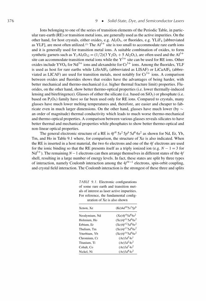
376 9 � Solid-State, Dye, and Semiconductor Lasers
Ions belonging to one of the series of transition elements of the Periodic Table, in partic-ular rare-earth (RE) or transition metal ions, are generally used as the active impurities. On theother hand, for host crystals, either oxides, e.g. Al2O3, or fluorides, e.g. YLiF4 [abbreviatedas YLF], are most often utilized..1/ The Al3C site is too small to accommodate rare earth ionsand it is generally used for transition metal ions. A suitable combination of oxides, to formsynthetic garnets such as Y3Al5O12 D .1=2/.3 Y2O3 C 5 Al2O3/, are often used and the Al3Csite can accommodate transition metal ions while the Y3C site can be used for RE ions. Otheroxides include YVO4 for Nd3C ions and alexandrite for Cr3C ions. Among the fluorides, YLFis used as host for rare earths while LiSrAlF6 (abbreviated as LISAF) or LiCaAlF6 (abbre-viated as LICAF) are used for transition metals, most notably for Cr3C ions. A comparisonbetween oxides and fluorides shows that oxides have the advantages of being harder, withbetter mechanical and thermo-mechanical (i.e. higher thermal fracture limit) properties. Flu-orides, on the other hand, show better thermo-optical properties (i.e. lower thermally-inducedlensing and birefringence). Glasses of either the silicate (i.e. based on SiO2) or phosphate (i.e.based on P2O5) family have so far been used only for RE ions. Compared to crystals, manyglasses have much lower melting temperatures and, therefore, are easier and cheaper to fab-ricate even in much larger dimensions. On the other hand, glasses have much lower (by �an order of magnitude) thermal conductivity which leads to much worse thermo-mechanicaland thermo-optical properties. A comparison between various glasses reveals silicates to havebetter thermal and mechanical properties while phosphates to show better thermo-optical andnon-linear optical properties.
The general electronic structure of a RE is 4f N 5s2 5p6 5d0 6s2 as shown for Nd, Er, Yb,Tm, and Ho in Table 9.1 where, for comparison, the structure of Xe is also indicated. Whenthe RE is inserted in a host material, the two 6s electrons and one of the 4f electrons are usedfor the ionic binding so that the RE presents itself as a triply ionized ion (e.g. N � 1 D 3 forNd3C). The remaining N �1 electrons can then arrange themselves in different states of the 4fshell, resulting in a large number of energy levels. In fact, these states are split by three typesof interaction, namely Coulomb interaction among the 4f N�1 electrons, spin-orbit coupling,and crystal field interaction. The Coulomb interaction is the strongest of these three and splits
TABLE 9.1. Electronic configurationsof some rare earth and transition met-als of interest as laser active impurities.For reference, the fundamental config-
uration of Xe is also shown
Xenon, Xe .Kr/4d105s25p6
Neodymium, Nd .Xe/4f 45d06s2
Holmium, Ho .Xe/4f 115d06s2
Erbium, Er .Xe/4f 125d06s2
Thulium, Tm .Xe/4f 135d06s2
Ytterbium, Yb .Xe/4f 145d06s2
Chromium, Cr .Ar/3d54s1
Titanium, Ti .Ar/3d24s2
Cobalt, Co .Ar/3d74s2
Nickel, Ni .Ar/3d84s2
9.2 � Solid-State Lasers 377
the 4f states into sublevels which are typically separated by � 10,000 cm�1. Spin-orbit cou-pling then splits each term into manifolds typically separated by � 3,000 cm�1. Crystal fieldinteraction produces the weakest perturbation (weakened by the screening effect of the 5s2
and 5p6 orbitals), thus further splitting each sub-level into a manifold with energy separationtypically of 200 cm�1. All relevant absorption and emission features are due to transitionsbetween these 4f states (4f –4f transitions). Electric dipole transitions within the 4f shell areparity-forbidden and it needs a mixture of wavefunctions with opposite parity, brought aboutby the crystal-field interaction, to create non-zero, although still weak, transition probabili-ties. Thus, one generally finds long (hundreds of �s) radiative lifetimes. Furthermore, due tothe screening from the 5s2 and 5p6 orbitals, electron-phonon coupling turns out to be veryweak. One thus has sharp transition lines and weak non-radiative decay channels for low ion-doping (ion-ion interaction can lead to non-radiative decay at high RE ion concentrations, seeFig. 2.13). From the above considerations one expects large values of the overall lifetime, � ,and of the product �� , where � is the peak cross-section. This implies a low threshold pumppower for laser action since, e.g. for a four level laser, the threshold pump rate is proportionalto 1=�� [see Eq. (7.3.3)].
The electronic configurations for those transition metals, of interest for laser action, arealso shown in Table 9.1. Note that the electronic configuration of the most important activespecies, i.e., Cr, is given by .Ar/3d54s1, while those of Ti, Co, and Ni can be written inthe general form .Ar/3dN4s2 (with N D 2 for Ti, 7 for Co and 8 for Ni). When in an ioniccrystal, the 4s1 electron and two 3d electrons of Cr are used for the ionic binding and Cr ispresent as a triply ionized ion with 3 electrons left in the 3d shell. For Titanium, the two 4selectrons and one 3d electron are used for the ionic binding and Ti is present as triply ionizedion with only one electron left in the 3d shell. For both Co and Ni the two 4s electrons areused for the binding and these elements are present as doubly ionized ions. In all cases, theremaining electrons in the 3d orbital can arrange themselves in a large number of states (e.g.24 for Cr3C) and all the absorption and emission features of transition metal ions arise from3d � 3d transitions. Lacking the screening which occurs for RE ions, the 3d states interactstrongly with the crystal field of the host and, as we shall see later, this is the fundamentalreason for the vibronic character, leading to wide absorption and emission bands, for most ofthe corresponding transitions. Again electric dipole transitions within the 3d shell are parityforbidden but, due to the stronger crystal field compared to the RE case, the 3d�3d transitionsare more allowed and thus the lifetimes are significantly shorter (a few �s) than those of the4f � 4f transitions of RE ions. Compared to e.g. Nd:YAG, the transition cross sections aresomewhat smaller so that the product �� is now typically one order of magnitude smaller.
As a conclusion to this section, it is worth noting that ions belonging to the actinideseries, notably U3C, were also used in the early days of laser development (actually theU3C laser was the second solid state laser to be developed, i.e. immediately after the rubylaser). These ions are essentially no longer used but they deserve a mention here for historicalreasons.
9.2.1. The Ruby Laser
This type of laser was the first to be made to operate (T. H. Maiman, June 1960.2,3/) andstill continues to be used in some applications..4/ As a naturally occurring precious stone, ruby
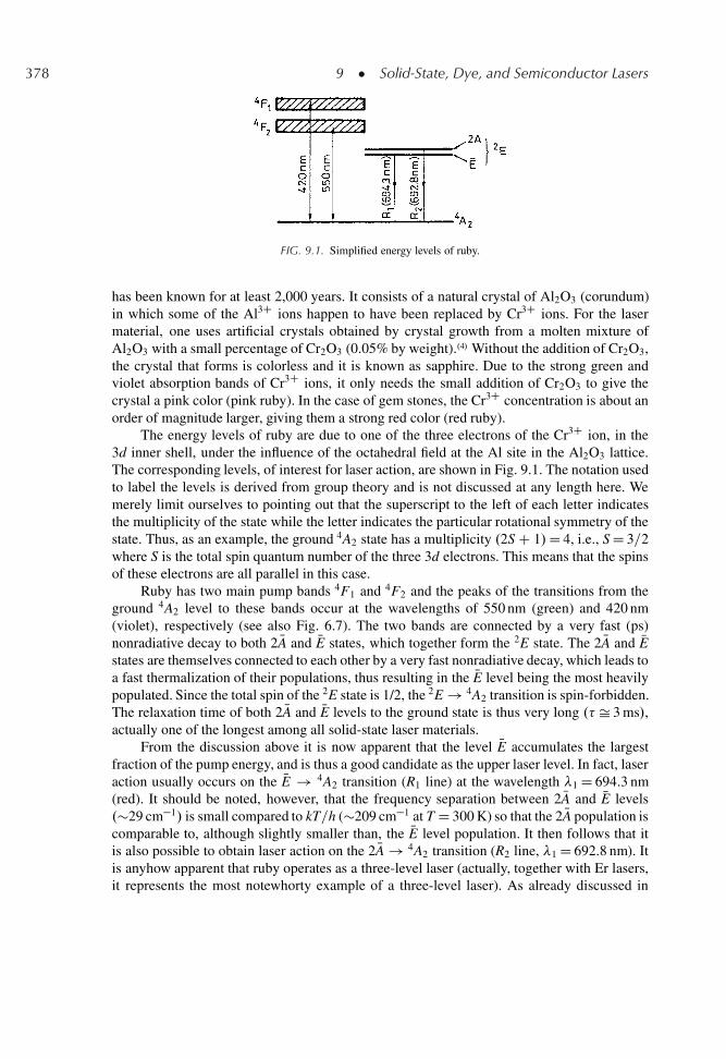
378 9 � Solid-State, Dye, and Semiconductor Lasers
FIG. 9.1. Simplified energy levels of ruby.
has been known for at least 2,000 years. It consists of a natural crystal of Al2O3 (corundum)in which some of the Al3C ions happen to have been replaced by Cr3C ions. For the lasermaterial, one uses artificial crystals obtained by crystal growth from a molten mixture ofAl2O3 with a small percentage of Cr2O3 (0.05% by weight)..4/ Without the addition of Cr2O3,the crystal that forms is colorless and it is known as sapphire. Due to the strong green andviolet absorption bands of Cr3C ions, it only needs the small addition of Cr2O3 to give thecrystal a pink color (pink ruby). In the case of gem stones, the Cr3C concentration is about anorder of magnitude larger, giving them a strong red color (red ruby).
The energy levels of ruby are due to one of the three electrons of the Cr3C ion, in the3d inner shell, under the influence of the octahedral field at the Al site in the Al2O3 lattice.The corresponding levels, of interest for laser action, are shown in Fig. 9.1. The notation usedto label the levels is derived from group theory and is not discussed at any length here. Wemerely limit ourselves to pointing out that the superscript to the left of each letter indicatesthe multiplicity of the state while the letter indicates the particular rotational symmetry of thestate. Thus, as an example, the ground 4A2 state has a multiplicity .2S C 1/D 4, i.e., S D 3=2where S is the total spin quantum number of the three 3d electrons. This means that the spinsof these electrons are all parallel in this case.
Ruby has two main pump bands 4F1 and 4F2 and the peaks of the transitions from theground 4A2 level to these bands occur at the wavelengths of 550 nm (green) and 420 nm(violet), respectively (see also Fig. 6.7). The two bands are connected by a very fast (ps)nonradiative decay to both 2 NA and NE states, which together form the 2E state. The 2 NA and NEstates are themselves connected to each other by a very fast nonradiative decay, which leads toa fast thermalization of their populations, thus resulting in the NE level being the most heavilypopulated. Since the total spin of the 2E state is 1/2, the 2E ! 4A2 transition is spin-forbidden.The relaxation time of both 2 NA and NE levels to the ground state is thus very long .� Š 3 ms/,actually one of the longest among all solid-state laser materials.
From the discussion above it is now apparent that the level NE accumulates the largestfraction of the pump energy, and is thus a good candidate as the upper laser level. In fact, laseraction usually occurs on the NE ! 4A2 transition (R1 line) at the wavelength �1 D 694.3 nm(red). It should be noted, however, that the frequency separation between 2 NA and NE levels.�29 cm�1/ is small compared to kT=h (�209 cm�1 at T D 300 K) so that the 2 NA population iscomparable to, although slightly smaller than, the NE level population. It then follows that itis also possible to obtain laser action on the 2 NA ! 4A2 transition (R2 line, �1 D 692.8 nm). Itis anyhow apparent that ruby operates as a three-level laser (actually, together with Er lasers,it represents the most notewhorty example of a three-level laser). As already discussed in
9.2 � Solid-State Lasers 379
TABLE 9.2. Optical and spectroscopic parametersof ruby for room temperature operation
Property Values and units
Cr2O3 doping 0.05 wt. %Cr3C concentration 1.58 1019 ions=cm3
Output wavelengths 694.3 nm (R1 line)692.9 nm (R2 line)
Upper laser level lifetime 3 msLinewidth of R1 laser transition 11 cm�1
Stim. emission cross-section �e 2.5 10�20 cm2
Absorption cross section �a 1.22 10�20 cm2
Refractive index .�D 694.3 nm/ n D 1.763 .E?c/n D 1.755 .Ej jc/
connection with Fig. 2.10, the R1 transition is, at room temperature, predominantly homoge-neously broadened, the broadening arising from the interaction of the Cr3C ions with latticephonons. The width of the transition (FWHM) is�0 Š 11 cm�1 (330 GHz) at T D 300 K. Asa summary, Table 9.2 shows some relevant optical and spectroscopic parameters of ruby atroom temperature.
Ruby lasers are usually operated in a pulsed regime. For this, the pump configurationof Fig. 6.1 using a medium-pressure .�500 Torr/ xenon flashtube, is generally utilized. Typ-ical rod diameters range between 5 and 10 mm with a length between 5 and 20 cm. It shouldbe noted that a helical flashtube surrounding the active rod was used in the earliest rubylasers. Since this laser operates on a three-level scheme, the threshold pump energy is typi-cally an order of magnitude higher than that of other solid-state lasers operating with four levelschemes (e.g. Neodimium lasers). Due to the long upper state lifetime, ruby lasers lend them-selves readily to Q-switched operation and, due to the relatively broad laser linewidth, theycan also produce short pulses .�5 � 10 ps/ in mode-locked operation. Both active and pas-sive methods can be used for Q-switching and mode-locking. When slow saturable absorbersare used for Q-switching, the laser tends to operate on a single transverse and longitudinalmode due to the mode selecting mechanism discussed in Sect. 8.4.2.4. With fast saturableabsorbers (usually solutions of cyanine dyes), simultaneous Q-switched and mode-lockedoperation occurs (see Fig. 8.28a). Peak powers of a few tens of MW, for Q-switching, anda few GW, when also mode-locked, are typical. Since the gain of the R2 line is somewhatsmaller than for the R1 line, laser action on the R2 line can be selected by using, for instance,the dispersive system of Fig. 7.16b. Ruby lasers can also run cw, transversely pumped by ahigh-pressure mercury lamp or longitudinally pumped by an Ar ion laser.
Ruby lasers, once very popular, are now less widely used since, on account of theirhigher threshold, they have been superseded by competitors, such as Nd:YAG or Nd:glasslasers. In fact, ruby lasers were extensively used in the past for the first mass production ofmilitary rangefinders, an application in which this laser is now completely replaced by othersolid-state lasers (Nd:YAG, Nd:glass, Yb:Er:glass). Ruby lasers are, however, still sometimesused for a number of scientific and technical applications where their shorter wavelength,compared to e.g., Nd:YAG, represents an important advantage. This is for instance the case
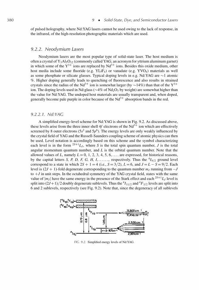
380 9 � Solid-State, Dye, and Semiconductor Lasers
of pulsed holography, where Nd:YAG lasers cannot be used owing to the lack of response, inthe infrared, of the high-resolution photographic materials which are used.
9.2.2. Neodymium Lasers
Neodymium lasers are the most popular type of solid-state laser. The host medium isoften a crystal of Y3Al5O12 (commonly called YAG, an acronym for yttrium aluminum garnet)in which some of the Y3C ions are replaced by Nd3C ions. Besides this oxide medium, otherhost media include some fluoride (e.g. YLiF4) or vanadate (e.g. YVO4) materials as wellas some phosphate or silicate glasses. Typical doping levels in e.g. Nd:YAG are �1 atomic%. Higher doping generally leads to quenching of fluorescence and also results in strainedcrystals since the radius of the Nd3C ion is somewhat larger (by �14%) than that of the Y3Cion. The doping levels used in Nd:glass (�4% of Nd2O3 by weight) are somewhat higher thanthe value for Nd:YAG. The undoped host materials are usually transparent and, when doped,generally become pale purple in color because of the Nd3C absorption bands in the red.
9.2.2.1. Nd:YAG
A simplified energy-level scheme for Nd:YAG is shown in Fig. 9.2. As discussed above,these levels arise from the three inner shell 4f electrons of the Nd3C ion which are effectivelyscreened by 8 outer electrons (5s2 and 5p6). The energy levels are only weakly influenced bythe crystal field of YAG and the Russell-Saunders coupling scheme of atomic physics can thenbe used. Level notation is accordingly based on this scheme and the symbol characterizingeach level is in the form 2SC1LJ, where S is the total spin quantum number, J is the totalangular momentum quantum number, and L is the orbital quantum number. Note that theallowed values of L, namely L D 0, 1, 2, 3, 4, 5, 6, . . . . are expressed, for historical reasons,by the capital letters S, P, D, F, G, H, I, . . . . . . , respectively. Thus the 4I9=2 ground levelcorrespond to a state in which 2S C 1 D 4 (i.e., S D 3=2), L D 6, and J D L � S D 9=2. Eachlevel is .2J C 1/-fold degenerate corresponding to the quantum number mJ running from �Jto CJ in unit steps. In the octahedral symmetry of the YAG crystal field, states with the samevalue of jmJ j have the same energy in the presence of the Stark effect and each 2SC1LJ level issplit into .2JC1/=2 doubly degenerate sublevels. Thus the 4I11=2 and 4F3=2 levels are split into6 and 2 sublevels, respectively (see Fig. 9.2). Note that, since the degeneracy of all sublevels
FIG. 9.2. Simplified energy levels of Nd:YAG.
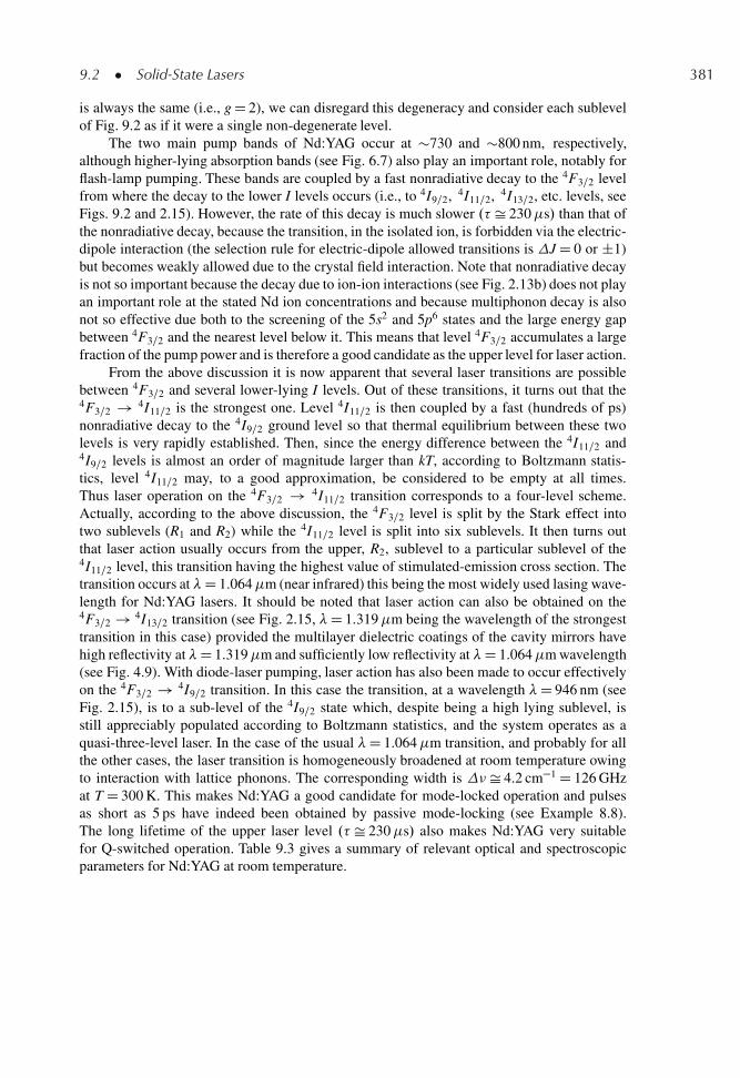
9.2 � Solid-State Lasers 381
is always the same (i.e., g D 2), we can disregard this degeneracy and consider each sublevelof Fig. 9.2 as if it were a single non-degenerate level.
The two main pump bands of Nd:YAG occur at �730 and �800 nm, respectively,although higher-lying absorption bands (see Fig. 6.7) also play an important role, notably forflash-lamp pumping. These bands are coupled by a fast nonradiative decay to the 4F3=2 levelfrom where the decay to the lower I levels occurs (i.e., to 4I9=2, 4I11=2, 4I13=2, etc. levels, seeFigs. 9.2 and 2.15). However, the rate of this decay is much slower .� Š 230�s/ than that ofthe nonradiative decay, because the transition, in the isolated ion, is forbidden via the electric-dipole interaction (the selection rule for electric-dipole allowed transitions is J D 0 or ˙1)but becomes weakly allowed due to the crystal field interaction. Note that nonradiative decayis not so important because the decay due to ion-ion interactions (see Fig. 2.13b) does not playan important role at the stated Nd ion concentrations and because multiphonon decay is alsonot so effective due both to the screening of the 5s2 and 5p6 states and the large energy gapbetween 4F3=2 and the nearest level below it. This means that level 4F3=2 accumulates a largefraction of the pump power and is therefore a good candidate as the upper level for laser action.
From the above discussion it is now apparent that several laser transitions are possiblebetween 4F3=2 and several lower-lying I levels. Out of these transitions, it turns out that the4F3=2 ! 4I11=2 is the strongest one. Level 4I11=2 is then coupled by a fast (hundreds of ps)nonradiative decay to the 4I9=2 ground level so that thermal equilibrium between these twolevels is very rapidly established. Then, since the energy difference between the 4I11=2 and4I9=2 levels is almost an order of magnitude larger than kT, according to Boltzmann statis-tics, level 4I11=2 may, to a good approximation, be considered to be empty at all times.Thus laser operation on the 4F3=2 ! 4I11=2 transition corresponds to a four-level scheme.Actually, according to the above discussion, the 4F3=2 level is split by the Stark effect intotwo sublevels (R1 and R2) while the 4I11=2 level is split into six sublevels. It then turns outthat laser action usually occurs from the upper, R2, sublevel to a particular sublevel of the4I11=2 level, this transition having the highest value of stimulated-emission cross section. Thetransition occurs at �D 1.064�m (near infrared) this being the most widely used lasing wave-length for Nd:YAG lasers. It should be noted that laser action can also be obtained on the4F3=2 ! 4I13=2 transition (see Fig. 2.15, �D 1.319�m being the wavelength of the strongesttransition in this case) provided the multilayer dielectric coatings of the cavity mirrors havehigh reflectivity at �D 1.319�m and sufficiently low reflectivity at �D 1.064�m wavelength(see Fig. 4.9). With diode-laser pumping, laser action has also been made to occur effectivelyon the 4F3=2 ! 4I9=2 transition. In this case the transition, at a wavelength �D 946 nm (seeFig. 2.15), is to a sub-level of the 4I9=2 state which, despite being a high lying sublevel, isstill appreciably populated according to Boltzmann statistics, and the system operates as aquasi-three-level laser. In the case of the usual �D 1.064�m transition, and probably for allthe other cases, the laser transition is homogeneously broadened at room temperature owingto interaction with lattice phonons. The corresponding width is �Š 4.2 cm�1 D 126 GHzat T D 300 K. This makes Nd:YAG a good candidate for mode-locked operation and pulsesas short as 5 ps have indeed been obtained by passive mode-locking (see Example 8.8).The long lifetime of the upper laser level .� Š 230�s/ also makes Nd:YAG very suitablefor Q-switched operation. Table 9.3 gives a summary of relevant optical and spectroscopicparameters for Nd:YAG at room temperature.
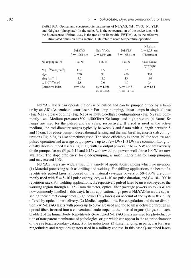
382 9 � Solid-State, Dye, and Semiconductor Lasers
TABLE 9.3. Optical and spectroscopic parameters of Nd:YAG, Nd : YVO4, Nd:YLF,and Nd:glass (phosphate). In the table, Nt is the concentration of the active ions, � isthe fluorescence lifetime, �0 is the transition linewidth (FWHM), �e is the effective
stimulated emission cross section. Data refer to room temperature operation
Nd:glassNd:YAG Nd : YVO4 Nd:YLF �D 1.054�m
�D 1.064�m �D 1.064�m �D 1.053�m (Phosphate)
Nd doping [at. %] 1 at. % 1 at. % 1 at. % 3.8% Nd2O3
by weightNt Œ1020 ions=cm3� 1.38 1.5 1.3 3.2� Œ�s� 230 98 450 300�0 Œcm�1� 4.5 11.3 13 180�e Œ10�19 cm2� 2.8 7.6 1.9 0.4Refractive index n D 1.82 no D 1.958 n0 D 1.4481 n D 1.54
ne D 2.168 ne D 1.4704
Nd:YAG lasers can operate either cw or pulsed and can be pumped either by a lampor by an AlGaAs semiconductor laser..5/ For lamp pumping, linear lamps in single-ellipse(Fig. 6.1a), close-coupling (Fig. 6.1b) or multiple-ellipse configurations (Fig. 6.2) are com-monly used. Medium pressure (500–1,500 Torr) Xe lamps and high-pressure (4–6 atm) Krlamps are used for the pulsed and cw cases, respectively. If a rod is used as the activemedium, the rod diameter ranges typically between 3 and 6 mm with a length between 5and 15 cm. To reduce pump-induced thermal lensing and thermal birefringence, a slab config-uration (Fig. 6.3a) is also sometimes used. The slope efficiency is about 3% for both cw andpulsed operation and average output powers up to a few kW (1–3 kW) are common. Longitu-dinally diode-pumped lasers (Fig. 6.11) with cw output powers up to �15 W and transverselydiode-pumped lasers (Figs. 6.14 and 6.15) with cw output powers well above 100 W are nowavailable. The slope efficiency, for diode-pumping, is much higher than for lamp pumpingand may exceed 10%.
Nd:YAG lasers are widely used in a variety of applications, among which we mention:(1) Material processing such as drilling and welding. For drilling applications the beam of arepetitively pulsed laser is focused on the material (average powers of 50–100 W are com-monly used with E D 5–10 J pulse energy,�p D 1–10 ms pulse duration, and f D 10–100 Hzrepetition rate). For welding applications, the repetitively pulsed laser beam is conveyed to theworking region through a, 0.5–2 mm diameter, optical fiber (average powers up to 2 kW arenow commonly handled in this way). In this application, high power Nd:YAG lasers are super-seding their direct competitors (high power CO2 lasers) on account of the system flexibilityoffered by optical fiber delivery. (2) Medical applications. For coagulation and tissue disrup-tion, cw Nd:YAG lasers with power up to 50 W are used and the beam is delivered through anoptical fiber, inserted into a conventional endoscope, to the internal organs (lungs, stomach,bladder) of the human body. Repetitively Q-switched Nd:YAG lasers are used for photodisrup-tion of transparent membranes of pathological origin which can appear in the anterior chamberof the eye (e.g., secondary cataract) or for iridoctomy. (3) Laser ranging, in particular for laserrangefinders and target designators used in a military contest. In this case Q-switched lasers
9.2 � Solid-State Lasers 383
are used .E � 100 mJ, �p D 5–20 ns, f D 1–20 Hz/. (4) Scientific applications: in this case,Q-switched lasers, with their second harmonic .�D 532 nm/, third harmonic .�Š 355 nm/and fourth-harmonic beams .�D 266 nm/, as well as mode-locked lasers are commonly usedin a variety of applications. Lastly, it should be noted that diode-pumped Nd:YAG lasers, withintracavity second harmonic generation, giving a green .�D 532 nm/ cw output power up to�10 W have become available, providing an all-solid-state alternative to the Ar laser for manyof its applications.
9.2.2.2. Nd:Glass.6/
As already mentioned, the relevant transitions of the Nd3C ion involve the three electronsof the 4f shell, and these are screened by 8 outer electrons in the 5s and 5p configuration.Accordingly, the energy levels of Nd:glass are approximately the same as those of Nd:YAG.Thus the strongest laser transition again occurs at about the same wavelength (�Š 1.054�mfor phosphate glass, see Table 9.3). The linewidths of the laser transitions are, however,much larger as a result of the inhomogeneous broadening arising from the local field inho-mogeneities typical of a glass medium. In particular the main �Š 1.054�m laser transition ismuch broader (by �40 times) while the peak cross section is somewhat smaller (by �7 times)than that of Nd:YAG. The larger bandwidth is of course a desirable feature for mode-lockedoperation and, indeed, diode-pumped passively-mode-locked Nd:glass lasers have producedultrashort pulses .�100 fs/. The smaller cross-section, on the other hand, is a desirable fea-ture for pulsed high-energy systems since the “threshold” inversion for the parasitic processof amplified spontaneous emission, ASE [see Eq. (2.9.4)], is correspondingly increased. Thusmore energy per unit volume can be stored in Nd:glass compared to Nd:YAG before the onsetof ASE [see Example 2.13]. It should also be noted that glass, due to its lower melting temper-ature, can be fabricated more easily than YAG and active media of much larger dimensionscan therefore be produced. Finally, since the pump absorption bands of Nd:glass are alsomuch broader than those of Nd:YAG and Nd3C concentrations are typically twice as great,the pumping efficiency of a lamp-pumped Nd:glass rod is somewhat larger (�1.6 times) thanthat of a Nd:YAG rod of the same dimensions (see Table 6.1). Against these advantages ofNd:glass compared to Nd:YAG, we must set the disadvantage arising from its much lowerthermal conductivity (thermal conductivity of glass is about ten times smaller than that ofNd:YAG). This has limited applications of Nd:glass lasers mainly to pulsed laser systems ofrather low repetition rate .<5 Hz/ so that thermal problems in the active medium (rod or slab)can be avoided�.
As discussed above, Nd:glass lasers are often used in applications where a pulsed laserof low repetition rate is required. This is for instance the case for some military rangefindersand some scientific Nd lasers. A very important application of Nd:glass is in the form of laseramplifiers in the very high energy systems used in laser-driven fusion experiments. Systemsbased on Nd:glass amplifiers have indeed been built in several countries, the largest one beingin the USA (Nova laser, Lawrence Livermore National Laboratory) and delivering pulses withenergy of �100 kJ and peak power of 100 TW .�p D 1 ns/. The laser makes use of a chain
� An exception to this is provided by glass fiber lasers, where long length and small transverse dimension eliminatethe thermal problem and have allowed cw outputs in excess of 100 W.
384 9 � Solid-State, Dye, and Semiconductor Lasers
of several Nd:glass amplifiers, the largest of which consists of Nd:glass disks (see Fig. 6.3b)of �4 cm in thickness and �75 cm in diameter. A national ignition facility delivering pulsesof much higher energy (�10 MJ, Lawrence Livermore National Laboratory) and a similarsystem delivering about the same output energy (�2 MJ, Limeil Center) are presently beingbuilt in the USA and in France, respectively.
9.2.2.3. Other Crystalline Hosts
Many other crystal materials have been used as hosts for the Nd3C ion and we limitourselves here to mentioning YLiF4 [YLF] and YVO4.
Compared to YAG, YLF has better thermo-optical properties.7/ (pump induced ther-mal lensing and thermal birefringence) and lamp pumped Nd:YLF lasers are used to obtainTEM00-mode cw-beams of better quality and higher output power. The larger linewidth ofNd:YLF compared to Nd:YAG (�3 times, see Table 9.3) makes Nd:YLF lasers particularlyattractive for mode-locked operation both with lamp and diode pumping (see Example 8.8).The mechanical and thermo-mechanical properties of YLF are however worse than those ofYAG and this make YLF rods more difficult to handle and easier to break. It should alsobe noted that the 1,053 nm emission wavelength of Nd:YLF provides a good match with thepeak gain wavelength of Nd:glass:phopsphate lasers (see Table 9.3). Mode-locked Nd:YLFlasers are accordingly used as the first stage in the large energy systems used for laser fusionexperiments.
Compared to Nd:YAG, Nd:YVO4 has much larger peak cross section .�e Š 7.6�10�19 cm2/ and much shorter fluorescence lifetime .� D 98�s/. The product �� is aboutthe same for the two cases and one thus expects approximately the same threshold. For agiven inversion, however, the gain coefficient of Nd:YVO4 is about 3 times larger than thatof Nd:YAG and this makes a Nd:YVO4 laser less sensitive to cavity losses. Longitudinally-diode-pumped Nd:YVO4 of high cw power .�15 W/ are now commercially available and, forthis application, Nd:YVO4 seems to be preferred to Nd:YAG.
9.2.3. Yb:YAG
The Yb:YAG laser is the most noteworthy example of a quasi-three level laser. It oscil-lates at �1.03�m wavelength and thus presents itself as direct competitor to Nd:YAG laser.Since it operates on a quasi-three-level laser scheme, it is usually pumped by semiconductorlaser diodes which can provide the intense pumping required..8/
A simplified scheme of the energy level diagram of Yb:YAG is shown in Fig. 9.3. Thelevel structure is particularly simple here, only one excited manifold, 2F5=2, being present,because Yb3C is one electron short to a full 4f shell (see Table 9.1), this shell thus actingas if it contained one electron hole. The two main absorption lines occur at 968 and 941 nm,respectively, the two lines have approximately the same value of the peak absorption crosssection, the line at 941 nm being usually preferred for diode-pumping due to its larger width.The main gain line occurs at 1.03�m (quasi-three-level laser). Table 9.4 shows some relevantoptical and spectroscopic parameters of Yb:YAG at room temperature. Note, in particular,the long lifetime, � D 1.16 ms, of essentially radiative origin, which is indicative of a goodstorage medium.
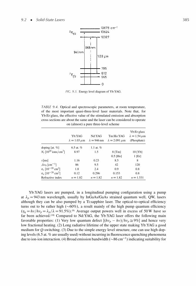
9.2 � Solid-State Lasers 385
FIG. 9.3. Energy level diagram of Yb:YAG.
TABLE 9.4. Optical and spectroscopic parameters, at room temperature,of the most important quasi-three-level laser materials. Note that, forYb:Er:glass, the effective value of the stimulated emission and absorptioncross sections are about the same and the laser can be considered to operate
on (almost) a pure three-level scheme
Yb:Er:glassYb:YAG Nd:YAG Tm:Ho:YAG �D 1.54�m
�D 1.03�m �D 946 nm �D 2.091�m (Phosphate)
doping [at. %] 6.5 at. % 1.1 at. %Nt Œ1020 ions=cm3� 8.97 1.5 8 [Tm] 10 [Yb]
0.5 [Ho] 1 [Er]� Œms� 1.16 0.23 8.5 8�0 Œcm�1� 86 9.5 42 120�e Œ10�20 cm2� 1.8 2.4 0.9 0.8�a Œ10�20 cm2� 0.12 0.296 0.153 0.8Refractive index n D 1.82 n D 1.82 n D 1.82 n D 1.531
Yb:YAG lasers are pumped, in a longitudinal pumping configuration using a pumpat �p D 943 nm wavelength, usually by InGaAs/GaAs strained quantum well, QW, lasersalthough they can be also pumped by a Ti:sapphire laser. The optical-to-optical efficiencyturns out to be rather high .�60%/, a result mainly of the high pump quantum efficiency.�q D h�=h�p D�p=�D 91.5%/..9/ Average output powers well in excess of 50 W have sofar been achieved..10/ Compared to Nd:YAG, the Yb:YAG laser offers the following mainfavorable properties: (1) Very low quantum defect Œ.h�p � h�/=h�p Š 9%� and hence verylow fractional heating. (2) Long radiative lifetime of the upper state making Yb:YAG a goodmedium for Q-switching. (3) Due to the simple energy level structure, one can use high dop-ing levels (6.5 at. % are usually used) without incurring in fluorescence quenching phenomenadue to ion-ion interaction. (4) Broad emission bandwidth .�86 cm�1/ indicating suitability for
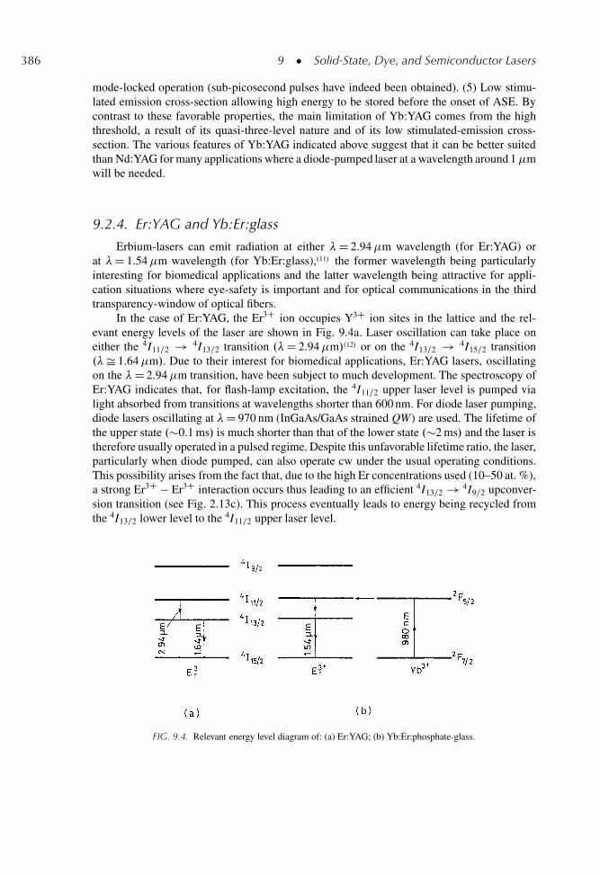
386 9 � Solid-State, Dye, and Semiconductor Lasers
mode-locked operation (sub-picosecond pulses have indeed been obtained). (5) Low stimu-lated emission cross-section allowing high energy to be stored before the onset of ASE. Bycontrast to these favorable properties, the main limitation of Yb:YAG comes from the highthreshold, a result of its quasi-three-level nature and of its low stimulated-emission cross-section. The various features of Yb:YAG indicated above suggest that it can be better suitedthan Nd:YAG for many applications where a diode-pumped laser at a wavelength around 1�mwill be needed.
9.2.4. Er:YAG and Yb:Er:glass
Erbium-lasers can emit radiation at either �D 2.94�m wavelength (for Er:YAG) orat �D 1.54�m wavelength (for Yb:Er:glass),.11/ the former wavelength being particularlyinteresting for biomedical applications and the latter wavelength being attractive for appli-cation situations where eye-safety is important and for optical communications in the thirdtransparency-window of optical fibers.
In the case of Er:YAG, the Er3C ion occupies Y3C ion sites in the lattice and the rel-evant energy levels of the laser are shown in Fig. 9.4a. Laser oscillation can take place oneither the 4I11=2 ! 4I13=2 transition .�D 2.94�m/.12/ or on the 4I13=2 ! 4I15=2 transition.�Š 1.64�m/. Due to their interest for biomedical applications, Er:YAG lasers, oscillatingon the �D 2.94�m transition, have been subject to much development. The spectroscopy ofEr:YAG indicates that, for flash-lamp excitation, the 4I11=2 upper laser level is pumped vialight absorbed from transitions at wavelengths shorter than 600 nm. For diode laser pumping,diode lasers oscillating at �D 970 nm (InGaAs/GaAs strained QW) are used. The lifetime ofthe upper state .�0.1 ms/ is much shorter than that of the lower state .�2 ms/ and the laser istherefore usually operated in a pulsed regime. Despite this unfavorable lifetime ratio, the laser,particularly when diode pumped, can also operate cw under the usual operating conditions.This possibility arises from the fact that, due to the high Er concentrations used (10–50 at. %),a strong Er3C � Er3C interaction occurs thus leading to an efficient 4I13=2 ! 4I9=2 upconver-sion transition (see Fig. 2.13c). This process eventually leads to energy being recycled fromthe 4I13=2 lower level to the 4I11=2 upper laser level.
FIG. 9.4. Relevant energy level diagram of: (a) Er:YAG; (b) Yb:Er:phosphate-glass.
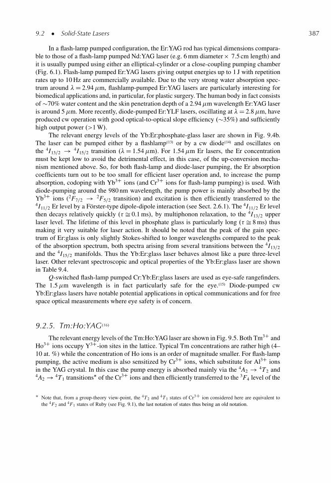
9.2 � Solid-State Lasers 387
In a flash-lamp pumped configuration, the Er:YAG rod has typical dimensions compara-ble to those of a flash-lamp pumped Nd:YAG laser (e.g. 6 mm diameter � 7.5 cm length) andit is usually pumped using either an elliptical-cylinder or a close-coupling pumping chamber(Fig. 6.1). Flash-lamp pumped Er:YAG lasers giving output energies up to 1 J with repetitionrates up to 10 Hz are commercially available. Due to the very strong water absorption spec-trum around �D 2.94�m, flashlamp-pumped Er:YAG lasers are particularly interesting forbiomedical applications and, in particular, for plastic surgery. The human body in fact consistsof �70% water content and the skin penetration depth of a 2.94�m wavelength Er:YAG laseris around 5�m. More recently, diode-pumped Er:YLF lasers, oscillating at �D 2.8�m, haveproduced cw operation with good optical-to-optical slope efficiency .�35%/ and sufficientlyhigh output power .>1 W/.
The relevant energy levels of the Yb:Er:phosphate-glass laser are shown in Fig. 9.4b.The laser can be pumped either by a flashlamp.13/ or by a cw diode.14/ and oscillates onthe 4I13=2 ! 4I15=2 transition .�D 1.54�m/. For 1.54�m Er lasers, the Er concentrationmust be kept low to avoid the detrimental effect, in this case, of the up-conversion mecha-nism mentioned above. So, for both flash-lamp and diode-laser pumping, the Er absorptioncoefficients turn out to be too small for efficient laser operation and, to increase the pumpabsorption, codoping with Yb3C ions (and Cr3C ions for flash-lamp pumping) is used. Withdiode-pumping around the 980 nm wavelength, the pump power is mainly absorbed by theYb3C ions (2F7=2 ! 2F5=2 transition) and excitation is then efficiently transferred to the4I11=2 Er level by a Forster-type dipole-dipole interaction (see Sect. 2.6.1). The 4I11=2 Er levelthen decays relatively quickly .� Š 0.1 ms/, by multiphonon relaxation, to the 4I13=2 upperlaser level. The lifetime of this level in phosphate glass is particularly long .� Š 8 ms/ thusmaking it very suitable for laser action. It should be noted that the peak of the gain spec-trum of Er:glass is only slightly Stokes-shifted to longer wavelengths compared to the peakof the absorption spectrum, both spectra arising from several transitions between the 4I13=2
and the 4I15=2 manifolds. Thus the Yb:Er:glass laser behaves almost like a pure three-levellaser. Other relevant spectroscopic and optical properties of the Yb:Er:glass laser are shownin Table 9.4.
Q-switched flash-lamp pumped Cr:Yb:Er:glass lasers are used as eye-safe rangefinders.The 1.5�m wavelength is in fact particularly safe for the eye..15/ Diode-pumped cwYb:Er:glass lasers have notable potential applications in optical communications and for freespace optical measurements where eye safety is of concern.
9.2.5. Tm:Ho:YAG.16/
The relevant energy levels of the Tm:Ho:YAG laser are shown in Fig. 9.5. Both Tm3C andHo3C ions occupy Y3C-ion sites in the lattice. Typical Tm concentrations are rather high (4–10 at. %) while the concentration of Ho ions is an order of magnitude smaller. For flash-lamppumping, the active medium is also sensitized by Cr3C ions, which substitute for Al3C ionsin the YAG crystal. In this case the pump energy is absorbed mainly via the 4A2 ! 4T2 and4A2 ! 4T1 transitions� of the Cr3C ions and then efficiently transferred to the 3F4 level of the
� Note that, from a group-theory view-point, the 4T2 and 4T1 states of Cr3C ion considered here are equivalent tothe 4F2 and 4F1 states of Ruby (see Fig. 9.1), the last notation of states thus being an old notation.
388 9 � Solid-State, Dye, and Semiconductor Lasers
FIG. 9.5. Relevant energy level diagram of Cr:Tm:Ho:YAG system.
Tm3C ion by a Forster-type ion-ion interaction. For cw diode-pumping, the 3F4 level of Tm3Cis directly pumped by AlGaAs semiconductor lasers at 785 nm wavelength, so that codopingwith Cr3C ions is not needed. For both flash-lamp and diode-laser pumping, excitation to the3F4 level of Tm3C ion is then followed by a cross-relaxation process, between adjacent ions,of the form Tm.3F4/C Tm.3H6/ ! 2Tm.3H4/. This process converts one excited Tm ion inthe 3F4 state into two excited Tm ions both in the 3H4 state. For the high Tm concentrationsbeing used, this cross-relaxation process becomes dominant over the 3F4 radiative decay andleads to an overall pump quantum efficiency of nearly 2. A fast spatial migration of the excitedenergy between Tm ions, again due to Forster-type ion-ion interaction, then occurs until theexcitation reaches a Tm ion very near to a Ho ion. In this case, energy transfer to the 5I7 levelof Ho occurs followed by laser action on the Ho3C 5I7 ! 5I8 transition. Laser action actuallyoccurs between the lowest sub-level of the 5I7 manifold to a sublevel, � 462 cm�1 above theground sub-level, of the 5I8 manifold at �D 2.08�m wavelength (quasi-three-level laser).Without Ho-doping, the crystal can lase on the 3H4 ! 3H6 Tm transition at �D 2.02�mwavelength.
When flash-lamp pumped, the active medium is in the form of a rod of the same typicaldimensions as those of the Er:YAG rod considered in the previous section, and again pumpedin an elliptical cylinder or close-coupling configuration (see Fig. 6.1). Output energies up to1 J in a �200�s long pulse, and a slope efficiency of up to 4% with a repetition rate below10 Hz, are typical laser operating figures. This laser may find interesting applications in thebiomedical field since biological tissue also has a strong absorption around 2�m (althoughless strong than at the 2.94�m wavelength of the Er-laser). When diode-pumped, a longitudi-nal pumping configuration such as that of Fig. 6.11a is often used. Given the strong absorptioncoefficient of Tm3C ions at the pump wavelength .˛p Š 6 cm�1/, the thickness of the activemedium is now typically 2–3 mm and the medium is generally cooled to low temperatures.�10 to �40 ıC/ to reduce the thermal population of the lower laser level.
Eye-safe coherent laser radar systems using Tm:Ho:YAG lasers are used for remotemeasurements of wind velocity in the atmosphere. This involves a single frequency diode-pumped Tm:Ho laser, used to injection-seed a flash-lamp-pumped, Pockels cell Q-switched,Cr:Tm:Ho:YAG slave oscillator.
9.2 � Solid-State Lasers 389
9.2.6. Fiber Lasers.17/
In a fiber laser the active medium is the core of the fiber, doped with a rare earth. Mostcommonly, this fiber is of a single mode type and is made of silica. The pump beam islaunched longitudinally along the fiber length and may be guided either by the core itselfas occurs for the laser mode (conventional single mode fiber laser) or by an inner claddingaround this core (double-clad fiber-laser). It should be noted that, although fiber lasers werefirst demonstrated in the early days of laser development,.18/ they have become of practi-cal interest only in recent years after the advent of suitable diode-lasers allowing efficientpumping and of the techniques for fabricating doped single-mode silica fibers.
In a conventional single-mode fiber, the transverse dimensions of both pump, wp, andlaser, w0, beams are comparable to the core radius a (typically a Š 2.5�m). Thus both wp
and w0 are 10–50 times smaller than the corresponding typical values of a bulk device (seeExamples 7.4 and 7.5). From either Eq. (6.3.20) or (6.3.25), holding for a 4-level and a quasi-3-level laser respectively, one sees that the threshold pump power, Pth, is proportional tow2
0 C w2p
�. Hence, for the same values of laser parameters (e.g. � , �e, �p, � for a 4-level
laser), Pth is expected to be smaller in a fiber laser compared to a bulk device by two tothree orders of magnitude. Thus, again according to examples 7.4 and 7.5, threshold pumppowers well below 1 mW are expected and indeed achieved in fiber lasers. This argumentalso shows that laser action can be obtained for active media of very low radiative quan-tum efficiency and hence of very short lifetime � . On the other hand, the expression for thelaser slope efficiency for a 4-level and for a quasi-three-level laser [the two are identical, seeEqs. (7.3.13) and (7.4.10)], turns out to be independent of the upper state lifetime and onlydependent on the pump efficiency �p. Thus, even for a transition with a low radiative quan-tum efficiency, a high laser slope efficiency can be obtained provided that most of the pumppower is absorbed (i.e., �p Š 1). So, transitions which look unpromising in bulk media canstill show a low enough threshold in a fiber to be diode-pumped and show a high slope effi-ciency. It should be noted that an interesting effect occurring at the high pump powers (upto �100 mW, see Sect. 6.3.1) available from single-transverse-mode diode lasers is groundstate depletion. Consider for instance a 4-level laser such as Nd:glass and let Fp be the pumpphoton flux (assumed, for simplicity, to be uniform in the core) and Ng and N2 the populationsof the ground level and upper laser level, respectively. In the absence of laser action and undercw conditions one can then simply write the following balance equation
�pFpNg D N2=� (9.2.1)
where σp is the pump absorption cross section and τ is the upper state lifetime. Thus, tohave Ng D N2 one must have Fp D .Ip=h�p/D .1=σpτ/, where Ip is the pump intensity andh�p is the energy of a pump photon. According to Fig. 6.8a and Table 9.3, we now take,for a Nd:silica fiber, �p D 2.8 � 10�20 cm2 and � D 300 μs. From the previous expression weget Ip D .h�p=�pτ/Š 25 kW=cm2 so that Pp D IpAcore Š 0.25 mW, where Acore is the area ofthe core, taken to be �10�7 cm2. Thus, in the example considered, more than half of theground-state population is raised to the upper laser level at pump powers below 1 mW. Giventhe ease with which pump-induced depletion of the ground-state population occurs, it followsthat typical pump powers can deplete absorption over lengths very much exceeding the small-signal extinction length (l D 1=˛p, where ˛p is the small-signal absorption coefficient at thepump wavelength). It can be shown in fact that, if the pump power exceeds this saturation
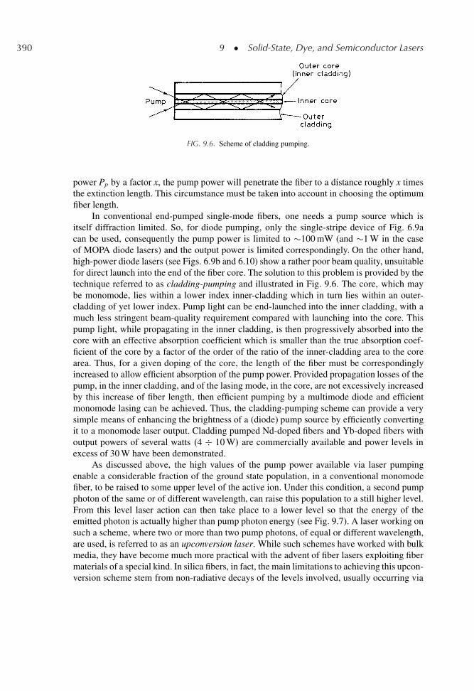
390 9 � Solid-State, Dye, and Semiconductor Lasers
FIG. 9.6. Scheme of cladding pumping.
power Pp by a factor x, the pump power will penetrate the fiber to a distance roughly x timesthe extinction length. This circumstance must be taken into account in choosing the optimumfiber length.
In conventional end-pumped single-mode fibers, one needs a pump source which isitself diffraction limited. So, for diode pumping, only the single-stripe device of Fig. 6.9acan be used, consequently the pump power is limited to �100 mW (and �1 W in the caseof MOPA diode lasers) and the output power is limited correspondingly. On the other hand,high-power diode lasers (see Figs. 6.9b and 6.10) show a rather poor beam quality, unsuitablefor direct launch into the end of the fiber core. The solution to this problem is provided by thetechnique referred to as cladding-pumping and illustrated in Fig. 9.6. The core, which maybe monomode, lies within a lower index inner-cladding which in turn lies within an outer-cladding of yet lower index. Pump light can be end-launched into the inner cladding, with amuch less stringent beam-quality requirement compared with launching into the core. Thispump light, while propagating in the inner cladding, is then progressively absorbed into thecore with an effective absorption coefficient which is smaller than the true absorption coef-ficient of the core by a factor of the order of the ratio of the inner-cladding area to the corearea. Thus, for a given doping of the core, the length of the fiber must be correspondinglyincreased to allow efficient absorption of the pump power. Provided propagation losses of thepump, in the inner cladding, and of the lasing mode, in the core, are not excessively increasedby this increase of fiber length, then efficient pumping by a multimode diode and efficientmonomode lasing can be achieved. Thus, the cladding-pumping scheme can provide a verysimple means of enhancing the brightness of a (diode) pump source by efficiently convertingit to a monomode laser output. Cladding pumped Nd-doped fibers and Yb-doped fibers withoutput powers of several watts .4 � 10 W/ are commercially available and power levels inexcess of 30 W have been demonstrated.
As discussed above, the high values of the pump power available via laser pumpingenable a considerable fraction of the ground state population, in a conventional monomodefiber, to be raised to some upper level of the active ion. Under this condition, a second pumpphoton of the same or of different wavelength, can raise this population to a still higher level.From this level laser action can then take place to a lower level so that the energy of theemitted photon is actually higher than pump photon energy (see Fig. 9.7). A laser working onsuch a scheme, where two or more than two pump photons, of equal or different wavelength,are used, is referred to as an upconversion laser. While such schemes have worked with bulkmedia, they have become much more practical with the advent of fiber lasers exploiting fibermaterials of a special kind. In silica fibers, in fact, the main limitations to achieving this upcon-version scheme stem from non-radiative decays of the levels involved, usually occurring via
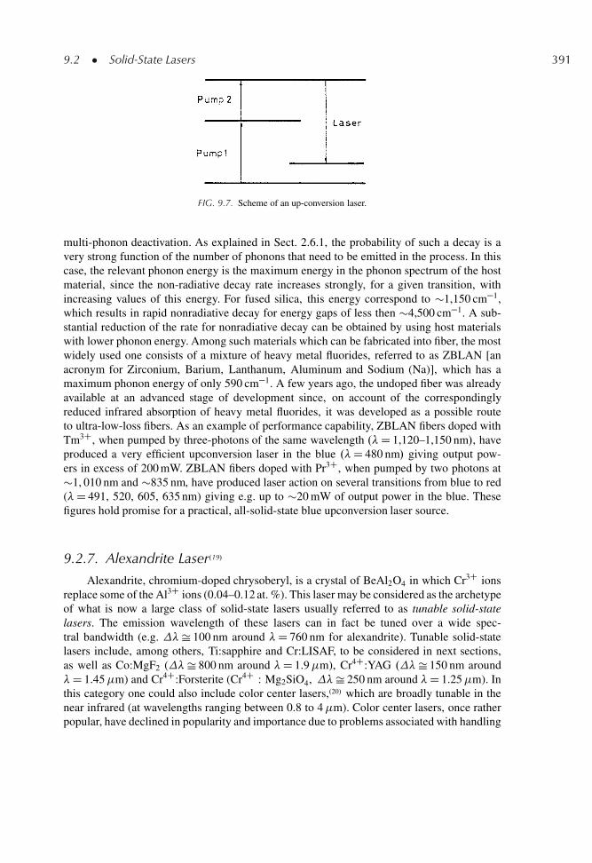
9.2 � Solid-State Lasers 391
FIG. 9.7. Scheme of an up-conversion laser.
multi-phonon deactivation. As explained in Sect. 2.6.1, the probability of such a decay is avery strong function of the number of phonons that need to be emitted in the process. In thiscase, the relevant phonon energy is the maximum energy in the phonon spectrum of the hostmaterial, since the non-radiative decay rate increases strongly, for a given transition, withincreasing values of this energy. For fused silica, this energy correspond to �1,150 cm�1,which results in rapid nonradiative decay for energy gaps of less then �4,500 cm�1. A sub-stantial reduction of the rate for nonradiative decay can be obtained by using host materialswith lower phonon energy. Among such materials which can be fabricated into fiber, the mostwidely used one consists of a mixture of heavy metal fluorides, referred to as ZBLAN [anacronym for Zirconium, Barium, Lanthanum, Aluminum and Sodium (Na)], which has amaximum phonon energy of only 590 cm�1. A few years ago, the undoped fiber was alreadyavailable at an advanced stage of development since, on account of the correspondinglyreduced infrared absorption of heavy metal fluorides, it was developed as a possible routeto ultra-low-loss fibers. As an example of performance capability, ZBLAN fibers doped withTm3C, when pumped by three-photons of the same wavelength .�D 1,120–1,150 nm/, haveproduced a very efficient upconversion laser in the blue .�D 480 nm/ giving output pow-ers in excess of 200 mW. ZBLAN fibers doped with Pr3C, when pumped by two photons at�1, 010 nm and �835 nm, have produced laser action on several transitions from blue to red(�D 491, 520, 605, 635 nm) giving e.g. up to �20 mW of output power in the blue. Thesefigures hold promise for a practical, all-solid-state blue upconversion laser source.
9.2.7. Alexandrite Laser.19/
Alexandrite, chromium-doped chrysoberyl, is a crystal of BeAl2O4 in which Cr3C ionsreplace some of the Al3C ions (0.04–0.12 at. %). This laser may be considered as the archetypeof what is now a large class of solid-state lasers usually referred to as tunable solid-statelasers. The emission wavelength of these lasers can in fact be tuned over a wide spec-tral bandwidth (e.g. �Š 100 nm around �D 760 nm for alexandrite). Tunable solid-statelasers include, among others, Ti:sapphire and Cr:LISAF, to be considered in next sections,as well as Co:MgF2 (�Š 800 nm around �D 1.9�m), Cr4C:YAG .�Š 150 nm around�D 1.45�m) and Cr4C:Forsterite (Cr4C : Mg2SiO4, �Š 250 nm around �D 1.25�m). Inthis category one could also include color center lasers,.20/ which are broadly tunable in thenear infrared (at wavelengths ranging between 0.8 to 4�m). Color center lasers, once ratherpopular, have declined in popularity and importance due to problems associated with handling
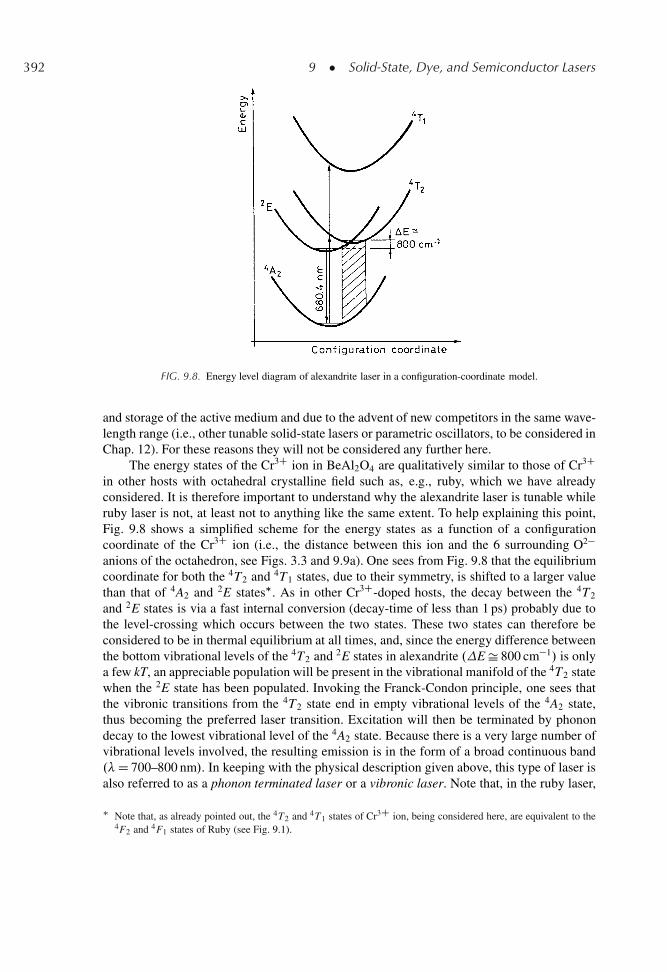
392 9 � Solid-State, Dye, and Semiconductor Lasers
FIG. 9.8. Energy level diagram of alexandrite laser in a configuration-coordinate model.
and storage of the active medium and due to the advent of new competitors in the same wave-length range (i.e., other tunable solid-state lasers or parametric oscillators, to be considered inChap. 12). For these reasons they will not be considered any further here.
The energy states of the Cr3C ion in BeAl2O4 are qualitatively similar to those of Cr3Cin other hosts with octahedral crystalline field such as, e.g., ruby, which we have alreadyconsidered. It is therefore important to understand why the alexandrite laser is tunable whileruby laser is not, at least not to anything like the same extent. To help explaining this point,Fig. 9.8 shows a simplified scheme for the energy states as a function of a configurationcoordinate of the Cr3C ion (i.e., the distance between this ion and the 6 surrounding O2�anions of the octahedron, see Figs. 3.3 and 9.9a). One sees from Fig. 9.8 that the equilibriumcoordinate for both the 4T2 and 4T1 states, due to their symmetry, is shifted to a larger valuethan that of 4A2 and 2E states�. As in other Cr3C-doped hosts, the decay between the 4T2
and 2E states is via a fast internal conversion (decay-time of less than 1 ps) probably due tothe level-crossing which occurs between the two states. These two states can therefore beconsidered to be in thermal equilibrium at all times, and, since the energy difference betweenthe bottom vibrational levels of the 4T2 and 2E states in alexandrite .E Š 800 cm�1/ is onlya few kT, an appreciable population will be present in the vibrational manifold of the 4T2 statewhen the 2E state has been populated. Invoking the Franck-Condon principle, one sees thatthe vibronic transitions from the 4T2 state end in empty vibrational levels of the 4A2 state,thus becoming the preferred laser transition. Excitation will then be terminated by phonondecay to the lowest vibrational level of the 4A2 state. Because there is a very large number ofvibrational levels involved, the resulting emission is in the form of a broad continuous band.�D 700–800 nm/. In keeping with the physical description given above, this type of laser isalso referred to as a phonon terminated laser or a vibronic laser. Note that, in the ruby laser,
� Note that, as already pointed out, the 4T2 and 4T1 states of Cr3C ion, being considered here, are equivalent to the4F2 and 4F1 states of Ruby (see Fig. 9.1).
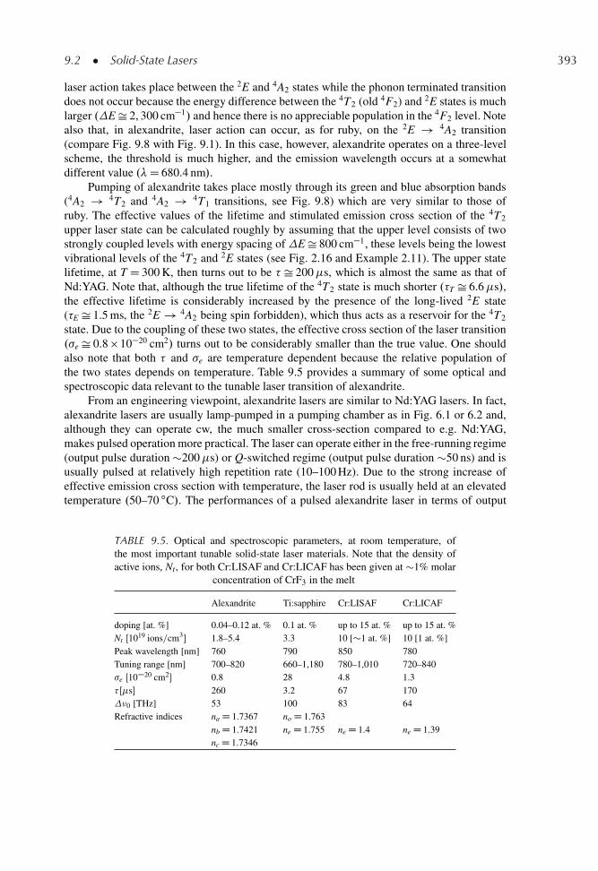
9.2 � Solid-State Lasers 393
laser action takes place between the 2E and 4A2 states while the phonon terminated transitiondoes not occur because the energy difference between the 4T2 (old 4F2) and 2E states is muchlarger .E Š 2, 300 cm�1/ and hence there is no appreciable population in the 4F2 level. Notealso that, in alexandrite, laser action can occur, as for ruby, on the 2E ! 4A2 transition(compare Fig. 9.8 with Fig. 9.1). In this case, however, alexandrite operates on a three-levelscheme, the threshold is much higher, and the emission wavelength occurs at a somewhatdifferent value .�D 680.4 nm/.
Pumping of alexandrite takes place mostly through its green and blue absorption bands(4A2 ! 4T2 and 4A2 ! 4T1 transitions, see Fig. 9.8) which are very similar to those ofruby. The effective values of the lifetime and stimulated emission cross section of the 4T2
upper laser state can be calculated roughly by assuming that the upper level consists of twostrongly coupled levels with energy spacing of E Š 800 cm�1, these levels being the lowestvibrational levels of the 4T2 and 2E states (see Fig. 2.16 and Example 2.11). The upper statelifetime, at T D 300 K, then turns out to be � Š 200�s, which is almost the same as that ofNd:YAG. Note that, although the true lifetime of the 4T2 state is much shorter .�T Š 6.6�s/,the effective lifetime is considerably increased by the presence of the long-lived 2E state(�E Š 1.5 ms, the 2E ! 4A2 being spin forbidden), which thus acts as a reservoir for the 4T2
state. Due to the coupling of these two states, the effective cross section of the laser transition.�e Š 0.8 � 10�20 cm2/ turns out to be considerably smaller than the true value. One shouldalso note that both � and �e are temperature dependent because the relative population ofthe two states depends on temperature. Table 9.5 provides a summary of some optical andspectroscopic data relevant to the tunable laser transition of alexandrite.
From an engineering viewpoint, alexandrite lasers are similar to Nd:YAG lasers. In fact,alexandrite lasers are usually lamp-pumped in a pumping chamber as in Fig. 6.1 or 6.2 and,although they can operate cw, the much smaller cross-section compared to e.g. Nd:YAG,makes pulsed operation more practical. The laser can operate either in the free-running regime(output pulse duration �200�s) or Q-switched regime (output pulse duration �50 ns) and isusually pulsed at relatively high repetition rate (10–100 Hz). Due to the strong increase ofeffective emission cross section with temperature, the laser rod is usually held at an elevatedtemperature .50–70 ıC/. The performances of a pulsed alexandrite laser in terms of output
TABLE 9.5. Optical and spectroscopic parameters, at room temperature, ofthe most important tunable solid-state laser materials. Note that the density ofactive ions, Nt, for both Cr:LISAF and Cr:LICAF has been given at �1% molar
concentration of CrF3 in the melt
Alexandrite Ti:sapphire Cr:LISAF Cr:LICAF
doping [at. %] 0.04–0.12 at. % 0.1 at. % up to 15 at. % up to 15 at. %Nt Œ1019 ions=cm3� 1.8–5.4 3.3 10 [�1 at. %] 10 [1 at. %]Peak wavelength [nm] 760 790 850 780Tuning range [nm] 700–820 660–1,180 780–1,010 720–840�e Œ10�20 cm2� 0.8 28 4.8 1.3� Œ�s� 260 3.2 67 170�0 [THz] 53 100 83 64Refractive indices na D 1.7367 no D 1.763
nb D 1.7421 ne D 1.755 ne D 1.4 ne D 1.39nc D 1.7346
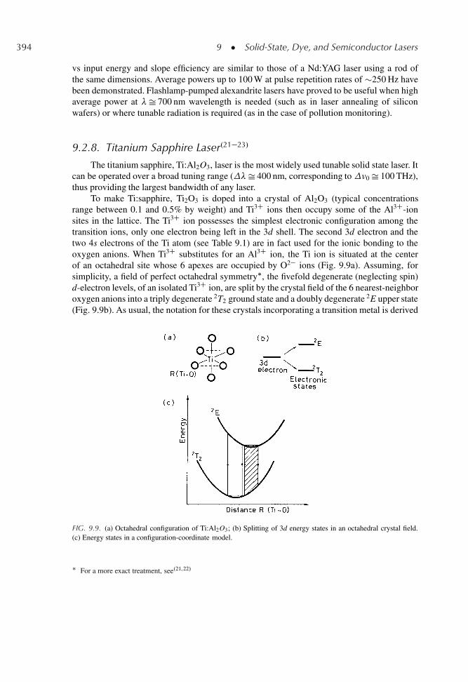
394 9 � Solid-State, Dye, and Semiconductor Lasers
vs input energy and slope efficiency are similar to those of a Nd:YAG laser using a rod ofthe same dimensions. Average powers up to 100 W at pulse repetition rates of �250 Hz havebeen demonstrated. Flashlamp-pumped alexandrite lasers have proved to be useful when highaverage power at �Š 700 nm wavelength is needed (such as in laser annealing of siliconwafers) or where tunable radiation is required (as in the case of pollution monitoring).
9.2.8. Titanium Sapphire Laser.21�23/
The titanium sapphire, Ti:Al2O3, laser is the most widely used tunable solid state laser. Itcan be operated over a broad tuning range (�Š 400 nm, corresponding to �0 Š 100 THz),thus providing the largest bandwidth of any laser.
To make Ti:sapphire, Ti2O3 is doped into a crystal of Al2O3 (typical concentrationsrange between 0.1 and 0.5% by weight) and Ti3C ions then occupy some of the Al3C-ionsites in the lattice. The Ti3C ion possesses the simplest electronic configuration among thetransition ions, only one electron being left in the 3d shell. The second 3d electron and thetwo 4s electrons of the Ti atom (see Table 9.1) are in fact used for the ionic bonding to theoxygen anions. When Ti3C substitutes for an Al3C ion, the Ti ion is situated at the centerof an octahedral site whose 6 apexes are occupied by O2� ions (Fig. 9.9a). Assuming, forsimplicity, a field of perfect octahedral symmetry�, the fivefold degenerate (neglecting spin)d-electron levels, of an isolated Ti3C ion, are split by the crystal field of the 6 nearest-neighboroxygen anions into a triply degenerate 2T2 ground state and a doubly degenerate 2E upper state(Fig. 9.9b). As usual, the notation for these crystals incorporating a transition metal is derived
FIG. 9.9. (a) Octahedral configuration of Ti:Al2O3; (b) Splitting of 3d energy states in an octahedral crystal field.(c) Energy states in a configuration-coordinate model.
� For a more exact treatment, see.21,22/
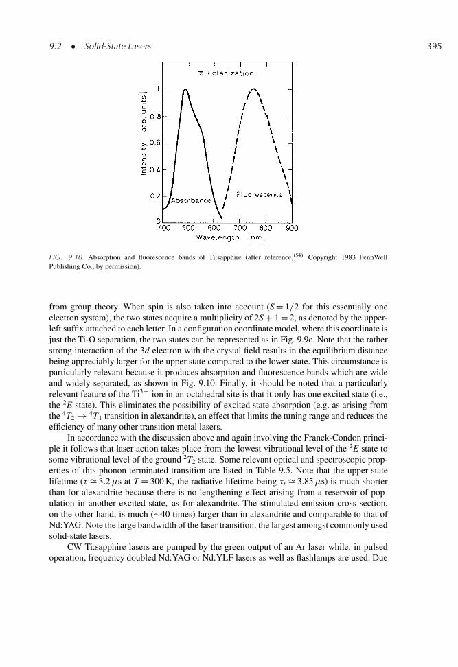
9.2 � Solid-State Lasers 395
FIG. 9.10. Absorption and fluorescence bands of Ti:sapphire (after reference,.54/ Copyright 1983 PennWellPublishing Co., by permission).
from group theory. When spin is also taken into account (S D 1=2 for this essentially oneelectron system), the two states acquire a multiplicity of 2S C 1 D 2, as denoted by the upper-left suffix attached to each letter. In a configuration coordinate model, where this coordinate isjust the Ti-O separation, the two states can be represented as in Fig. 9.9c. Note that the ratherstrong interaction of the 3d electron with the crystal field results in the equilibrium distancebeing appreciably larger for the upper state compared to the lower state. This circumstance isparticularly relevant because it produces absorption and fluorescence bands which are wideand widely separated, as shown in Fig. 9.10. Finally, it should be noted that a particularlyrelevant feature of the Ti3C ion in an octahedral site is that it only has one excited state (i.e.,the 2E state). This eliminates the possibility of excited state absorption (e.g. as arising fromthe 4T2 ! 4T1 transition in alexandrite), an effect that limits the tuning range and reduces theefficiency of many other transition metal lasers.
In accordance with the discussion above and again involving the Franck-Condon princi-ple it follows that laser action takes place from the lowest vibrational level of the 2E state tosome vibrational level of the ground 2T2 state. Some relevant optical and spectroscopic prop-erties of this phonon terminated transition are listed in Table 9.5. Note that the upper-statelifetime (� Š 3.2�s at T D 300 K, the radiative lifetime being �r Š 3.85�s) is much shorterthan for alexandrite because there is no lengthening effect arising from a reservoir of pop-ulation in another excited state, as for alexandrite. The stimulated emission cross section,on the other hand, is much (�40 times) larger than in alexandrite and comparable to that ofNd:YAG. Note the large bandwidth of the laser transition, the largest amongst commonly usedsolid-state lasers.
CW Ti:sapphire lasers are pumped by the green output of an Ar laser while, in pulsedoperation, frequency doubled Nd:YAG or Nd:YLF lasers as well as flashlamps are used. Due
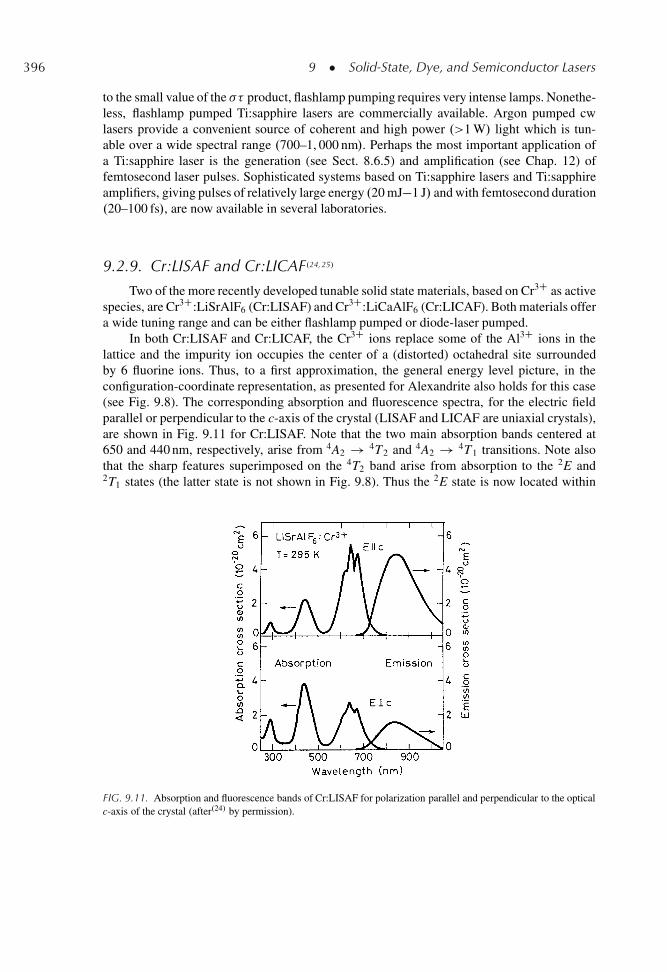
396 9 � Solid-State, Dye, and Semiconductor Lasers
to the small value of the �� product, flashlamp pumping requires very intense lamps. Nonethe-less, flashlamp pumped Ti:sapphire lasers are commercially available. Argon pumped cwlasers provide a convenient source of coherent and high power .>1 W/ light which is tun-able over a wide spectral range .700–1, 000 nm/. Perhaps the most important application ofa Ti:sapphire laser is the generation (see Sect. 8.6.5) and amplification (see Chap. 12) offemtosecond laser pulses. Sophisticated systems based on Ti:sapphire lasers and Ti:sapphireamplifiers, giving pulses of relatively large energy .20 mJ�1 J/ and with femtosecond duration.20–100 fs/, are now available in several laboratories.
9.2.9. Cr:LISAF and Cr:LICAF.24,25/
Two of the more recently developed tunable solid state materials, based on Cr3C as activespecies, are Cr3C:LiSrAlF6 (Cr:LISAF) and Cr3C:LiCaAlF6 (Cr:LICAF). Both materials offera wide tuning range and can be either flashlamp pumped or diode-laser pumped.
In both Cr:LISAF and Cr:LICAF, the Cr3C ions replace some of the Al3C ions in thelattice and the impurity ion occupies the center of a (distorted) octahedral site surroundedby 6 fluorine ions. Thus, to a first approximation, the general energy level picture, in theconfiguration-coordinate representation, as presented for Alexandrite also holds for this case(see Fig. 9.8). The corresponding absorption and fluorescence spectra, for the electric fieldparallel or perpendicular to the c-axis of the crystal (LISAF and LICAF are uniaxial crystals),are shown in Fig. 9.11 for Cr:LISAF. Note that the two main absorption bands centered at650 and 440 nm, respectively, arise from 4A2 ! 4T2 and 4A2 ! 4T1 transitions. Note alsothat the sharp features superimposed on the 4T2 band arise from absorption to the 2E and2T1 states (the latter state is not shown in Fig. 9.8). Thus the 2E state is now located within
FIG. 9.11. Absorption and fluorescence bands of Cr:LISAF for polarization parallel and perpendicular to the opticalc-axis of the crystal (after.24/ by permission).
9.3 � Dye Lasers 397
the 4A2 ! 4T2 absorption band which implies that the lowest vibrational level of 4T2 mustnow be located appreciably below the 2E state. Due to the fast relaxation between the twostates, it then follows that the most heavily populated state is now 4T2, so that the 2E statedoes not play any role as an energy reservoir, as for alexandrite. This is also evidenced bythe fact that the lifetime of the 4T2 state has been measured to be roughly independent oftemperature. Other relevant optical and spectroscopic parameters of the two laser materialsare listed in Table 9.5. Note that, amongst the tunable solid state laser materials shown inthe Table, Cr:LISAF exhibits the largest value of the �� product. Thus, due to its largervalues of both the cross section and the �� product and its wider tuning range (the tuningrange of Cr:LICAF is limited by excited state absorption), Cr:LISAF is generally preferred toCr:LICAF.
Cr:LISAF has found applications as a flashlamp or diode-pumped laser source providingtunability around 850 nm. The large gain linewidth makes this medium attractive for the gen-eration of femtosecond pulses. For this application, Kerr-lens mode locked Cr:LISAF lasers,end-pumped by GaInP/AlGaInP QW laser diodes at 670 nm wavelength, in a configurationsuch as that shown in Fig. 8.31, have been developed. Large, flashlamp pumped, Cr:LISAFamplifier systems, to amplify femtosecond pulses from either a Ti:sapphire or a Cr:LISAFmode-locked laser, have also been developed. Other potential applications of Cr:LISAF are intunable systems for pollution monitoring and for spectroscopy.
9.3. DYE LASERS.26/
Dye lasers make use of an active medium consisting of a solution of an organic dyein a liquid solvent such as ethyl or methyl alcohol, glycerol, or water. Organic dyes con-stitute a large class of polyatomic molecules containing long chains of conjugated doublebonds [e.g., .–C D/n]. Laser dyes usually belong to one of the following classes: (1) Poly-methine dyes, which provide laser oscillation in the red or near infrared .0.7–1.5�m/. As anexample Fig. 9.12a shows the chemical structure of the dye 3, 30 diethyl thiatricarbocyanineiodide, which oscillates in the infrared (at a peak wavelength, �p D 810 nm). (2) Xanthenedyes, whose laser operation is in the visible. As an example Fig. 9.12b shows the chemi-cal structure of the widely used rhodamine 6G dye .�p D 590 nm/. (3) Coumarin dyes, whichoscillate in the blue-green region (400–500 nm). As an example Fig. 9.12c shows the chemicalstructure of coumarin 2, which oscillates in the blue .�p D 450 nm/.
9.3.1. Photophysical Properties of Organic Dyes
Organic dyes usually show wide absorption and fluorescence bands without sharp fea-tures, the fluorescence being Stokes-shifted to longer wavelengths than the absorption, afeature reminiscent of the tunable solid state laser materials considered in the previoussections. As an example, Fig 9.13 shows the relevant absorption and emission characteristicsof rhodamine 6G in ethanol solution.
To understand the origin of the features shown in Fig. 9.13, we first need to considerthe energy levels of a dye molecule. A simple understanding of these levels can be obtainedusing the so-called free-electron model,.27/ which is illustrated here by considering the case
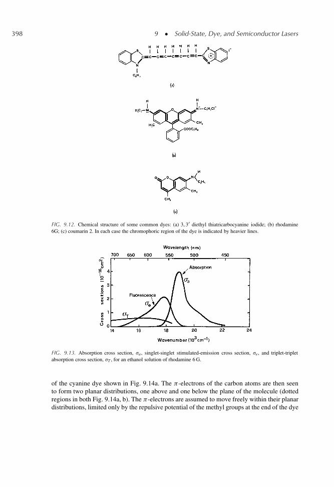
398 9 � Solid-State, Dye, and Semiconductor Lasers
FIG. 9.12. Chemical structure of some common dyes: (a) 3, 30 diethyl thiatricarbocyanine iodide; (b) rhodamine6G; (c) coumarin 2. In each case the chromophoric region of the dye is indicated by heavier lines.
FIG. 9.13. Absorption cross section, �a , singlet-singlet stimulated-emission cross section, �e, and triplet-tripletabsorption cross section, �T , for an ethanol solution of rhodamine 6 G.
of the cyanine dye shown in Fig. 9.14a. The -electrons of the carbon atoms are then seento form two planar distributions, one above and one below the plane of the molecule (dottedregions in both Fig. 9.14a, b). The -electrons are assumed to move freely within their planardistributions, limited only by the repulsive potential of the methyl groups at the end of the dye
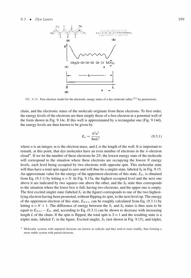
9.3 � Dye Lasers 399
FIG. 9.14. Free-electron model for the electronic energy states of a dye molecule (after,.27/ by permission).
chain, and the electronic states of the molecule originate from these electrons. To first order,the energy levels of the electrons are then simply those of a free electron in a potential well ofthe form shown in Fig. 9.14c. If this well is approximated by a rectangular one (Fig. 9.14d),the energy levels are then known to be given by
En D h2n2
8mL2(9.3.1)
where n is an integer, m is the electron mass, and L is the length of the well. It is important toremark, at this point, that dye molecules have an even number of electrons in the -electroncloud�. If we let the number of these electrons be 2N, the lowest energy state of the moleculewill correspond to the situation where these electrons are occupying the lowest N energylevels, each level being occupied by two electrons with opposite spin. This molecular statewill thus have a total spin equal to zero and will thus be a singlet state, labeled S0 in Fig. 9.15.An approximate value for the energy of the uppermost electrons of this state, EN , is obtainedfrom Eq. (9.3.1) by letting n D N. In Fig. 9.15a, the highest occupied level and the next oneabove it are indicated by two squares one above the other, and the S0 state thus correspondsto the situation where the lower box is full, having two electrons, and the upper one is empty.The first excited singlet state (labeled S1 in the figure) corresponds to one of the two highest-lying electron having been promoted, without flipping its spin, to the next level up. The energyof the uppermost electron of this state, ENC1, can be roughly calculated from Eq. (9.3.1) byletting n D N C 1. The difference of energy between the S1 and S0 states is thus seen to beequal to ENC1 � EN , and, according to Eq. (9.3.1) can be shown to decrease with increasinglength L of the chain. If the spin is flipped, the total spin is S D 1 and the resulting state is atriplet state, labeled T1 in the figure. Excited singlet, S2 (not shown in Fig. 9.15), and triplet,
� Molecular systems with unpaired electrons are known as radicals and they tend to react readily, thus forming amore stable system with paired electrons.
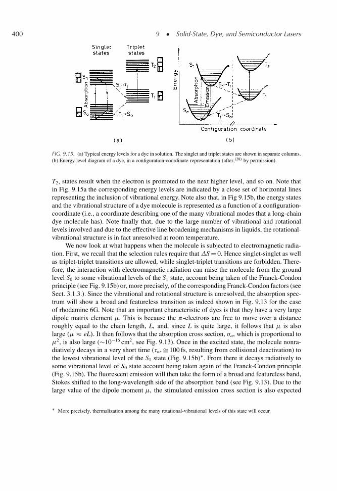
400 9 � Solid-State, Dye, and Semiconductor Lasers
FIG. 9.15. (a) Typical energy levels for a dye in solution. The singlet and triplet states are shown in separate columns.(b) Energy level diagram of a dye, in a configuration-coordinate representation (after,.28/ by permission).
T2, states result when the electron is promoted to the next higher level, and so on. Note thatin Fig. 9.15a the corresponding energy levels are indicated by a close set of horizontal linesrepresenting the inclusion of vibrational energy. Note also that, in Fig 9.15b, the energy statesand the vibrational structure of a dye molecule is represented as a function of a configuration-coordinate (i.e., a coordinate describing one of the many vibrational modes that a long-chaindye molecule has). Note finally that, due to the large number of vibrational and rotationallevels involved and due to the effective line broadening mechanisms in liquids, the rotational-vibrational structure is in fact unresolved at room temperature.
We now look at what happens when the molecule is subjected to electromagnetic radia-tion. First, we recall that the selection rules require that S D 0. Hence singlet-singlet as wellas triplet-triplet transitions are allowed, while singlet-triplet transitions are forbidden. There-fore, the interaction with electromagnetic radiation can raise the molecule from the groundlevel S0 to some vibrational levels of the S1 state, account being taken of the Franck-Condonprinciple (see Fig. 9.15b) or, more precisely, of the corresponding Franck-Condon factors (seeSect. 3.1.3.). Since the vibrational and rotational structure is unresolved, the absorption spec-trum will show a broad and featureless transition as indeed shown in Fig. 9.13 for the caseof rhodamine 6G. Note that an important characteristic of dyes is that they have a very largedipole matrix element �. This is because the -electrons are free to move over a distanceroughly equal to the chain length, L, and, since L is quite large, it follows that � is alsolarge .� � eL/. It then follows that the absorption cross section, �a, which is proportional to�2, is also large (�10�16 cm2, see Fig. 9.13). Once in the excited state, the molecule nonra-diatively decays in a very short time (�nr Š 100 fs, resulting from collisional deactivation) tothe lowest vibrational level of the S1 state (Fig. 9.15b)�. From there it decays radiatively tosome vibrational level of S0 state account being taken again of the Franck-Condon principle(Fig. 9.15b). The fluorescent emission will then take the form of a broad and featureless band,Stokes shifted to the long-wavelength side of the absorption band (see Fig. 9.13). Due to thelarge value of the dipole moment �, the stimulated emission cross section is also expected
� More precisely, thermalization among the many rotational-vibrational levels of this state will occur.
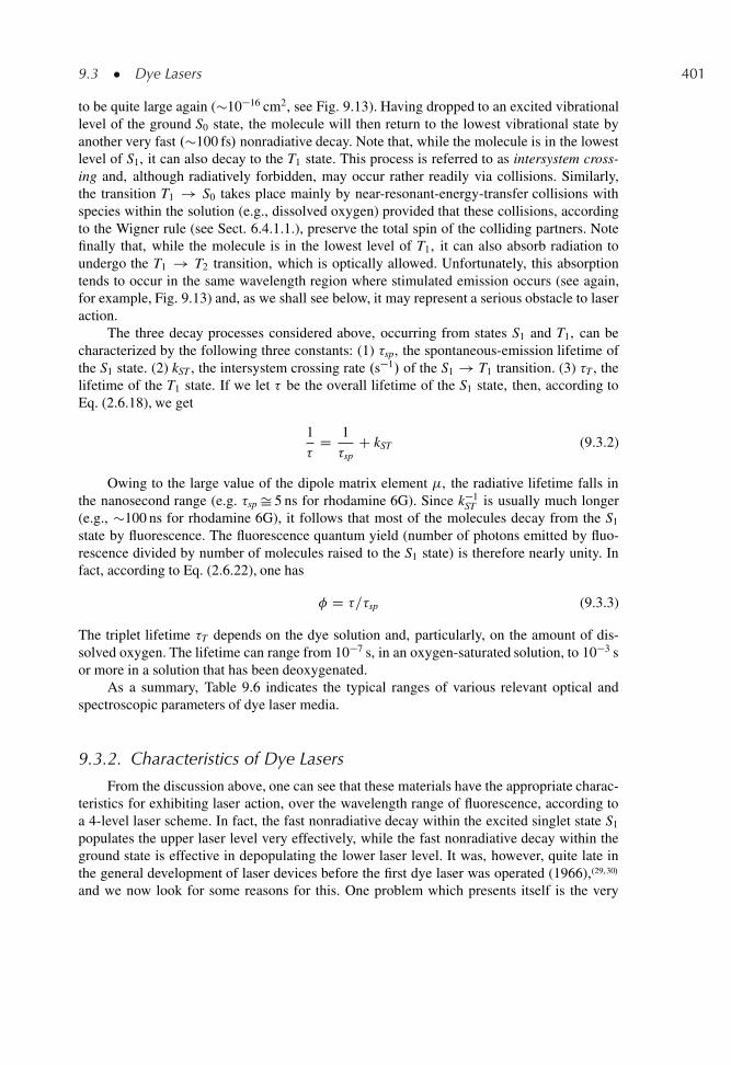
9.3 � Dye Lasers 401
to be quite large again (�10�16 cm2, see Fig. 9.13). Having dropped to an excited vibrationallevel of the ground S0 state, the molecule will then return to the lowest vibrational state byanother very fast .�100 fs/ nonradiative decay. Note that, while the molecule is in the lowestlevel of S1, it can also decay to the T1 state. This process is referred to as intersystem cross-ing and, although radiatively forbidden, may occur rather readily via collisions. Similarly,the transition T1 ! S0 takes place mainly by near-resonant-energy-transfer collisions withspecies within the solution (e.g., dissolved oxygen) provided that these collisions, accordingto the Wigner rule (see Sect. 6.4.1.1.), preserve the total spin of the colliding partners. Notefinally that, while the molecule is in the lowest level of T1, it can also absorb radiation toundergo the T1 ! T2 transition, which is optically allowed. Unfortunately, this absorptiontends to occur in the same wavelength region where stimulated emission occurs (see again,for example, Fig. 9.13) and, as we shall see below, it may represent a serious obstacle to laseraction.
The three decay processes considered above, occurring from states S1 and T1, can becharacterized by the following three constants: (1) �sp, the spontaneous-emission lifetime ofthe S1 state. (2) kST , the intersystem crossing rate .s�1/ of the S1 ! T1 transition. (3) �T , thelifetime of the T1 state. If we let � be the overall lifetime of the S1 state, then, according toEq. (2.6.18), we get
1
�D 1
�spC kST (9.3.2)
Owing to the large value of the dipole matrix element �, the radiative lifetime falls inthe nanosecond range (e.g. �sp Š 5 ns for rhodamine 6G). Since k�1
ST is usually much longer(e.g., �100 ns for rhodamine 6G), it follows that most of the molecules decay from the S1
state by fluorescence. The fluorescence quantum yield (number of photons emitted by fluo-rescence divided by number of molecules raised to the S1 state) is therefore nearly unity. Infact, according to Eq. (2.6.22), one has
� D �=�sp (9.3.3)
The triplet lifetime �T depends on the dye solution and, particularly, on the amount of dis-solved oxygen. The lifetime can range from 10�7 s, in an oxygen-saturated solution, to 10�3 sor more in a solution that has been deoxygenated.
As a summary, Table 9.6 indicates the typical ranges of various relevant optical andspectroscopic parameters of dye laser media.
9.3.2. Characteristics of Dye Lasers
From the discussion above, one can see that these materials have the appropriate charac-teristics for exhibiting laser action, over the wavelength range of fluorescence, according toa 4-level laser scheme. In fact, the fast nonradiative decay within the excited singlet state S1
populates the upper laser level very effectively, while the fast nonradiative decay within theground state is effective in depopulating the lower laser level. It was, however, quite late inthe general development of laser devices before the first dye laser was operated (1966),.29,30/
and we now look for some reasons for this. One problem which presents itself is the very
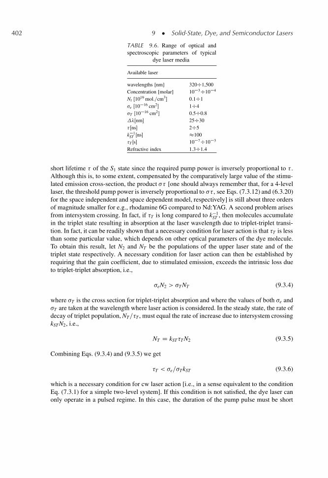
402 9 � Solid-State, Dye, and Semiconductor Lasers
TABLE 9.6. Range of optical andspectroscopic parameters of typical
dye laser media
Available laser
wavelengths [nm] 320�1,500Concentration [molar] 10�3�10�4
Nt Œ1019 mol.=cm3� 0.1�1�e Œ10�16 cm2� 1�4�T Œ10�16 cm2� 0.5�0.8�Œnm� 25�30� Œns� 2�5k�1
ST Œns� �100�T Œs� 10�7�10�3
Refractive index 1.3�1.4
short lifetime � of the S1 state since the required pump power is inversely proportional to � .Although this is, to some extent, compensated by the comparatively large value of the stimu-lated emission cross-section, the product �� [one should always remember that, for a 4-levellaser, the threshold pump power is inversely proportional to �� , see Eqs. (7.3.12) and (6.3.20)for the space independent and space dependent model, respectively] is still about three ordersof magnitude smaller for e.g., rhodamine 6G compared to Nd:YAG. A second problem arisesfrom intersystem crossing. In fact, if �T is long compared to k�1
ST , then molecules accumulatein the triplet state resulting in absorption at the laser wavelength due to triplet-triplet transi-tion. In fact, it can be readily shown that a necessary condition for laser action is that �T is lessthan some particular value, which depends on other optical parameters of the dye molecule.To obtain this result, let N2 and NT be the populations of the upper laser state and of thetriplet state respectively. A necessary condition for laser action can then be established byrequiring that the gain coefficient, due to stimulated emission, exceeds the intrinsic loss dueto triplet-triplet absorption, i.e.,
�eN2 > �TNT (9.3.4)
where �T is the cross section for triplet-triplet absorption and where the values of both �e and�T are taken at the wavelength where laser action is considered. In the steady state, the rate ofdecay of triplet population, NT=�T , must equal the rate of increase due to intersystem crossingkSTN2, i.e.,
NT D kST�TN2 (9.3.5)
Combining Eqs. (9.3.4) and (9.3.5) we get
�T < �e=�TkST (9.3.6)
which is a necessary condition for cw laser action [i.e., in a sense equivalent to the conditionEq. (7.3.1) for a simple two-level system]. If this condition is not satisfied, the dye laser canonly operate in a pulsed regime. In this case, the duration of the pump pulse must be short
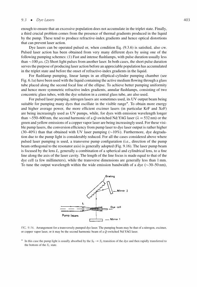
9.3 � Dye Lasers 403
enough to ensure that an excessive population does not accumulate in the triplet state. Finally,a third crucial problem comes from the presence of thermal gradients produced in the liquidby the pump. These tend to produce refractive-index gradients and hence optical distortionsthat can prevent laser action.
Dye lasers can be operated pulsed or, when condition Eq. (9.3.6) is satisfied, also cw.Pulsed laser action has been obtained from very many different dyes by using one of thefollowing pumping schemes: (1) Fast and intense flashlamps, with pulse duration usually lessthan �100�s. (2) Short light pulses from another laser. In both cases, the short pulse durationserves the purpose of producing laser action before an appreciable population has accumulatedin the triplet state and before the onset of refractive-index gradients in the liquid.
For flashlamp pumping, linear lamps in an elliptical-cylinder pumping chamber (seeFig. 6.1a) have been used with the liquid containing the active medium flowing through a glasstube placed along the second focal line of the ellipse. To achieve better pumping uniformityand hence more symmetric refractive index gradients, annular flashlamps, consisting of twoconcentric glass tubes, with the dye solution in a central glass tube, are also used.
For pulsed laser pumping, nitrogen lasers are sometimes used, its UV output beam beingsuitable for pumping many dyes that oscillate in the visible range�. To obtain more energyand higher average power, the more efficient excimer lasers (in particular KrF and XeF)are being increasingly used as UV pumps, while, for dyes with emission wavelength longerthan �550–600 nm, the second harmonic of a Q-switched Nd:YAG laser .�D 532 nm/ or thegreen and yellow emissions of a copper vapor laser are being increasingly used. For these visi-ble pump lasers, the conversion efficiency from pump laser to dye laser output is rather higher(30–40%) than that obtained with UV laser pumping .�10%/. Furthermore, dye degrada-tion due to the pump light is considerably reduced. For all the cases considered above wherepulsed laser pumping is used, a transverse pump configuration (i.e., direction of the pumpbeam orthogonal to the resonator axis) is generally adopted (Fig. 9.16). The laser pump beamis focused by the lens L, generally a combination of a spherical and cylindrical lens, to a fineline along the axis of the laser cavity. The length of the line focus is made equal to that of thedye cell (a few millimeters), while the transverse dimensions are generally less than 1 mm.To tune the output wavelength within the wide emission bandwidth of a dye .�30–50 nm/,
FIG. 9.16. Arrangement for a transversely pumped dye laser. The pumping beam may be that of a nitrogen, excimer,or copper vapor laser, or it may be the second harmonic beam of a Q-switched Nd:YAG laser.
� In this case the pump light is usually absorbed by the S0 ! S2 transition of the dye and then rapidly transferred tothe bottom of the S1 state.
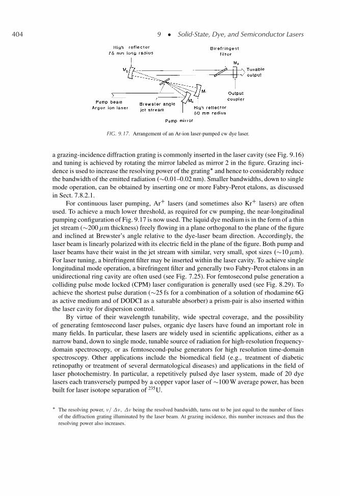
404 9 � Solid-State, Dye, and Semiconductor Lasers
FIG. 9.17. Arrangement of an Ar-ion laser-pumped cw dye laser.
a grazing-incidence diffraction grating is commonly inserted in the laser cavity (see Fig. 9.16)and tuning is achieved by rotating the mirror labeled as mirror 2 in the figure. Grazing inci-dence is used to increase the resolving power of the grating� and hence to considerably reducethe bandwidth of the emitted radiation .�0.01–0.02 nm/. Smaller bandwidths, down to singlemode operation, can be obtained by inserting one or more Fabry-Perot etalons, as discussedin Sect. 7.8.2.1.
For continuous laser pumping, ArC lasers (and sometimes also KrC lasers) are oftenused. To achieve a much lower threshold, as required for cw pumping, the near-longitudinalpumping configuration of Fig. 9.17 is now used. The liquid dye medium is in the form of a thinjet stream (�200�m thickness) freely flowing in a plane orthogonal to the plane of the figureand inclined at Brewster’s angle relative to the dye-laser beam direction. Accordingly, thelaser beam is linearly polarized with its electric field in the plane of the figure. Both pump andlaser beams have their waist in the jet stream with similar, very small, spot sizes .�10�m/.For laser tuning, a birefringent filter may be inserted within the laser cavity. To achieve singlelongitudinal mode operation, a birefringent filter and generally two Fabry-Perot etalons in anunidirectional ring cavity are often used (see Fig. 7.25). For femtosecond pulse generation acolliding pulse mode locked (CPM) laser configuration is generally used (see Fig. 8.29). Toachieve the shortest pulse duration (�25 fs for a combination of a solution of rhodamine 6Gas active medium and of DODCI as a saturable absorber) a prism-pair is also inserted withinthe laser cavity for dispersion control.
By virtue of their wavelength tunability, wide spectral coverage, and the possibilityof generating femtosecond laser pulses, organic dye lasers have found an important role inmany fields. In particular, these lasers are widely used in scientific applications, either as anarrow band, down to single mode, tunable source of radiation for high-resolution frequency-domain spectroscopy, or as femtosecond-pulse generators for high resolution time-domainspectroscopy. Other applications include the biomedical field (e.g., treatment of diabeticretinopathy or treatment of several dermatological diseases) and applications in the field oflaser photochemistry. In particular, a repetitively pulsed dye laser system, made of 20 dyelasers each transversely pumped by a copper vapor laser of �100 W average power, has beenbuilt for laser isotope separation of 235U.
� The resolving power, �= �, � being the resolved bandwidth, turns out to be just equal to the number of linesof the diffraction grating illuminated by the laser beam. At grazing incidence, this number increases and thus theresolving power also increases.
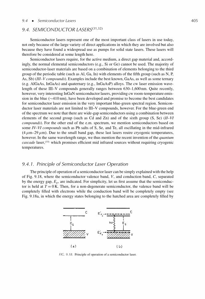
9.4 � Semiconductor Lasers 405
9.4. SEMICONDUCTOR LASERS.31,32/
Semiconductor lasers represent one of the most important class of lasers in use today,not only because of the large variety of direct applications in which they are involved but alsobecause they have found a widespread use as pumps for solid state lasers. These lasers willtherefore be considered at some length here.
Semiconductor lasers require, for the active medium, a direct gap material and, accord-ingly, the normal elemental semiconductors (e.g., Si or Ge) cannot be used. The majority ofsemiconductor-laser materials are based on a combination of elements belonging to the thirdgroup of the periodic table (such as Al, Ga, In) with elements of the fifth group (such as N, P,As, Sb) (III–V compounds). Examples include the best known, GaAs, as well as some ternary(e.g. AlGaAs, InGaAs) and quaternary (e.g., InGaAsP) alloys. The cw laser emission wave-length of these III–V compounds generally ranges between 630–1,600nm. Quite recently,however, very interesting InGaN semiconductor lasers, providing cw room-temperature emis-sion in the blue .�410 nm/, have been developed and promise to become the best candidatesfor semiconductor laser emission in the very important blue-green spectral region. Semicon-ductor laser materials are not limited to III–V compounds, however. For the blue-green endof the spectrum we note that there are wide-gap semiconductors using a combination betweenelements of the second group (such as Cd and Zn) and of the sixth group (S, Se) (II–VIcompounds). For the other end of the e.m. spectrum, we mention semiconductors based onsome IV–VI compounds such as Pb salts of S, Se, and Te, all oscillating in the mid-infrared.4�m–29�m/. Due to the small band gap, these last lasers reuire cryogenic temperatures,however. In the same wavelength range, we thus mention the recent invention of the quantumcascade laser,.33/ which promises efficient mid infrared sources without requiring cryogenictemperatures.
9.4.1. Principle of Semiconductor Laser Operation
The principle of operation of a semiconductor laser can be simply explained with the helpof Fig. 9.18, where the semiconductor valence band, V , and conduction band, C, separatedby the energy gap, Eg, are indicated. For simplicity, let us first assume that the semiconduc-tor is held at T D 0 K. Then, for a non-degenerate semiconductor, the valence band will becompletely filled with electrons while the conduction band will be completely empty (seeFig. 9.18a, in which the energy states belonging to the hatched area are completely filled by
FIG. 9.18. Principle of operation of a semiconductor laser.
406 9 � Solid-State, Dye, and Semiconductor Lasers
electrons). Suppose now that some electrons are raised from the valence band to the conduc-tion band by a suitable pumping mechanism. After a very short time .�1 ps/, the electronsin the conduction band drop to the lowest unoccupied levels of this band, and, meanwhile,any electron near the top of the valence band also drops to the lowest unoccupied levels ofthis band, thus leaving holes at the top of the valence band (Fig. 9.18b). This situation can bedescribed by introducing the quasi-Fermi levels, E0
Fc, for the conduction band and, E0
Fv, for the
valence band (see Sect. 3.2.3.). At T D 0 K they define, for each band, the energy below whichstates are fully occupied by electrons and above which, states are empty. Light emission cannow occur when an electron, of the conduction band, falls back to the valence band recom-bining with a hole. This, so-called recombination-radiation process, is the process by whichradiation is emitted in light emitting diodes (LED). Given the appropriate conditions, how-ever, a process of stimulated emission of this recombination radiation, thus leading to laseraction, can occur. It was shown in Sect. 3.2.5. that the condition for a photon to be amplifiedrather than absorbed by the semiconductor is simply given by [see Eq. (3.2.39)]
Eg h� E0Fc
� E0Fv
(9.4.1)
In the simple case where T D 0 K, this condition can be readily understood from Fig. 9.18b,since the non-hatched area in the valence band corresponds to states which are empty, anda conduction band electron can only fall into an empty state of the valence band. However,the detailed treatment of Sect. 3.2.5. shows that condition of Eq. (9.4.1) in fact holds forany temperature and simply means that, for the range of transition energy h� defined byEq. (9.4.1), the gain arising from stimulated emission exceeds the absorption. To achievecondition of Eq. (9.4.1) one must, of course, have E0
Fc� E0
Fv Eg. It is important at this point
to realize that the values of both E0Fc
and E0Fv
depend on the intensity of the pumping process,i.e. on the number density, N, of electrons raised to the conduction band (see Fig. 3.15).Actually E0
FcD E0
Fc.N/ increases while E0
FvD E0
Fv.N/ decreases as N is increased. Thus, to
obtain E0Fc
� E0Fv
Eg i.e., to have gain exceeding absorption losses, the electron density Nmust exceed some critical value established by the condition
E0Fc.N/ � E0
Fv.N/ D Eg (9.4.2)
The value of the injected carrier density which satisfies Eq. (9.4.2) is referred to as the carrierdensity at transparency�, Ntr . If now the injected carrier density is larger than Ntr, the semi-conductor will exhibit a net gain and, if this active medium is placed in a suitable cavity, laseraction can occur if this net gain is sufficient to overcome the cavity losses. Thus, to obtainlaser action, the injected carriers must reach some threshold value, Nth, larger than Ntr by asufficient margin to allow the net gain to overcome the cavity losses.
Semiconductor laser pumping can in principle be achieved, and indeed has beenachieved, in a number of ways, e.g., by using either the beam of another laser, or an aux-iliary electron beam, to transversely or longitudinally excite a bulk semiconductor. By far themost convenient way of excitation is, however, to use the semiconductor laser in the form of adiode with excitation produced by current flowing in the forward direction of the junction..34/
Laser action in a semiconductor was in fact first observed in 1962 by using a p-n junction
� Condition (9.4.2) is thus equivalent to the condition N2 D N1 under which a non-degenerate two level systembecomes transparent
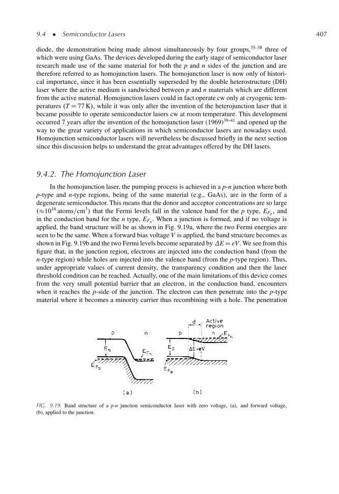
9.4 � Semiconductor Lasers 407
diode, the demonstration being made almost simultaneously by four groups,35–38 three ofwhich were using GaAs. The devices developed during the early stage of semiconductor laserresearch made use of the same material for both the p and n sides of the junction and aretherefore referred to as homojunction lasers. The homojunction laser is now only of histori-cal importance, since it has been essentially superseded by the double heterostructure (DH)laser where the active medium is sandwiched between p and n materials which are differentfrom the active material. Homojunction lasers could in fact operate cw only at cryogenic tem-peratures .T D 77 K/, while it was only after the invention of the heterojunction laser that itbecame possible to operate semiconductor lasers cw at room temperature. This developmentoccurred 7 years after the invention of the homojunction laser (1969)39–41 and opened up theway to the great variety of applications in which semiconductor lasers are nowadays used.Homojunction semiconductor lasers will nevertheless be discussed briefly in the next sectionsince this discussion helps to understand the great advantages offered by the DH lasers.
9.4.2. The Homojunction Laser
In the homojunction laser, the pumping process is achieved in a p-n junction where bothp-type and n-type regions, being of the same material (e.g., GaAs), are in the form of adegenerate semiconductor. This means that the donor and acceptor concentrations are so large.�1018 atoms=cm3/ that the Fermi levels fall in the valence band for the p type, EFp , andin the conduction band for the n type, EFn . When a junction is formed, and if no voltage isapplied, the band structure will be as shown in Fig. 9.19a, where the two Fermi energies areseen to be the same. When a forward bias voltage V is applied, the band structure becomes asshown in Fig. 9.19b and the two Fermi levels become separated byE D eV . We see from thisfigure that, in the junction region, electrons are injected into the conduction band (from then-type region) while holes are injected into the valence band (from the p-type region). Thus,under appropriate values of current density, the transparency condition and then the laserthreshold condition can be reached. Actually, one of the main limitations of this device comesfrom the very small potential barrier that an electron, in the conduction band, encounterswhen it reaches the p-side of the junction. The electron can then penetrate into the p-typematerial where it becomes a minority carrier thus recombining with a hole. The penetration
FIG. 9.19. Band structure of a p-n junction semiconductor laser with zero voltage, (a), and forward voltage,(b), applied to the junction.
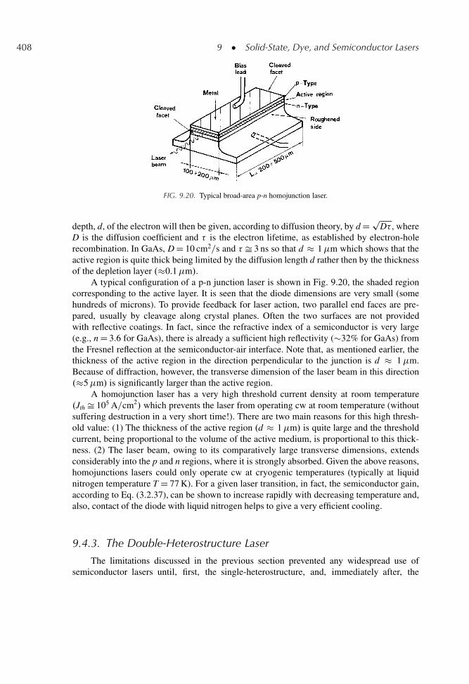
408 9 � Solid-State, Dye, and Semiconductor Lasers
FIG. 9.20. Typical broad-area p-n homojunction laser.
depth, d, of the electron will then be given, according to diffusion theory, by d D pD� , where
D is the diffusion coefficient and � is the electron lifetime, as established by electron-holerecombination. In GaAs, D D 10 cm2=s and � Š 3 ns so that d � 1�m which shows that theactive region is quite thick being limited by the diffusion length d rather then by the thicknessof the depletion layer .�0.1�m/.
A typical configuration of a p-n junction laser is shown in Fig. 9.20, the shaded regioncorresponding to the active layer. It is seen that the diode dimensions are very small (somehundreds of microns). To provide feedback for laser action, two parallel end faces are pre-pared, usually by cleavage along crystal planes. Often the two surfaces are not providedwith reflective coatings. In fact, since the refractive index of a semiconductor is very large(e.g., n D 3.6 for GaAs), there is already a sufficient high reflectivity (�32% for GaAs) fromthe Fresnel reflection at the semiconductor-air interface. Note that, as mentioned earlier, thethickness of the active region in the direction perpendicular to the junction is d � 1�m.Because of diffraction, however, the transverse dimension of the laser beam in this direction.�5�m/ is significantly larger than the active region.
A homojunction laser has a very high threshold current density at room temperature.Jth Š 105 A=cm2/ which prevents the laser from operating cw at room temperature (withoutsuffering destruction in a very short time!). There are two main reasons for this high thresh-old value: (1) The thickness of the active region .d � 1�m/ is quite large and the thresholdcurrent, being proportional to the volume of the active medium, is proportional to this thick-ness. (2) The laser beam, owing to its comparatively large transverse dimensions, extendsconsiderably into the p and n regions, where it is strongly absorbed. Given the above reasons,homojunctions lasers could only operate cw at cryogenic temperatures (typically at liquidnitrogen temperature T D 77 K). For a given laser transition, in fact, the semiconductor gain,according to Eq. (3.2.37), can be shown to increase rapidly with decreasing temperature and,also, contact of the diode with liquid nitrogen helps to give a very efficient cooling.
9.4.3. The Double-Heterostructure Laser
The limitations discussed in the previous section prevented any widespread use ofsemiconductor lasers until, first, the single-heterostructure, and, immediately after, the
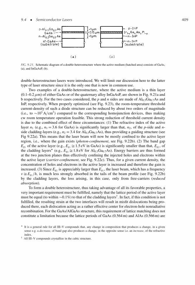
9.4 � Semiconductor Lasers 409
FIG. 9.21. Schematic diagram of a double-heterostructure where the active medium (hatched area) consists of GaAs,(a), and InGaAsP, (b).
double-heterostructure lasers were introduced. We will limit our discussion here to the lattertype of laser structure since it is the only one that is now in common use.
Two examples of a double-heterostructure, where the active medium is a thin layer.0.1–0.2�m/ of either GaAs or of the quaternary alloy InGaAsP, are shown in Fig. 9.21a andb respectively. For the two cases considered, the p and n sides are made of Al0.3Ga0.7As andInP, respectively. When properly optimized (see Fig. 9.23), the room-temperature thresholdcurrent-density of such a diode structure can be reduced by about two orders of magnitude(i.e., to �103 A=cm2) compared to the corresponding homojunction devices, thus makingcw room temperature operation feasible. This strong reduction of threshold current densityis due to the combined effect of three circumstances: (1) The refractive index of the activelayer n1 (e.g., n1 D 3.6 for GaAs) is significantly larger than that, n2, of the p-side and n-side cladding-layers (e.g., n2 D 3.4 for Al0.3Ga0.7As), thus providing a guiding structure (seeFig 9.22a). This means that the laser beam will now be mostly confined to the active layerregion, i.e., where the gain exists (photon-confinement, see Fig. 9.22b). (2) The band gapEg1 of the active layer (e.g., Eg1 Š 1.5 eV in GaAs) is significantly smaller than that, Eg2 , ofthe cladding layers� (e.g., Eg2 Š 1.8 eV for Al0.3Ga0.7As). Energy barriers are thus formedat the two junction planes thus effectively confining the injected holes and electrons withinthe active layer (carrier-confinement, see Fig. 9.22c). Thus, for a given current density, theconcentration of holes and electrons in the active layer is increased and therefore the gain isincreased. (3) Since Eg2 is appreciably larger than Eg1 , the laser beam, which has a frequency�Š Eg1=h, is much less strongly absorbed in the tails of the beam profile (see Fig. 9.22b)by the cladding layers, the loss arising, in this case, only from free-carriers (reducedabsorption).
To form a double heterostructure, thus taking advantage of all its favorable properties, avery important requirement must be fulfilled, namely that the lattice period of the active layermust be equal (to within �0.1%) to that of the cladding layers�. In fact, if this condition is notfulfilled, the resulting strain at the two interfaces will result in misfit dislocations being pro-duced there, each dislocation acting as a rather effective center for electron-hole nonradiativerecombination. For the GaAs/AlGaAs structure, this requirement of lattice matching does notconstitute a limitation because the lattice periods of GaAs (0.564 m) and AlAs (0.566 m) are
� It is a general rule for all III–V compounds that, any change in composition that produces a change, in a givensense e.g. a decrease, of band gap also produces a change, in the opposite sense i.e. an increase, of the refractiveindex.
� All III–V compounds crystallize in the cubic structure.
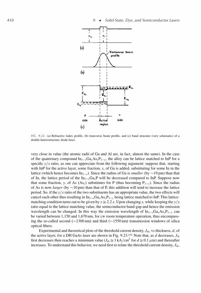
410 9 � Solid-State, Dye, and Semiconductor Lasers
FIG. 9.22. (a) Refractive index profile, (b) transverse beam profile, and (c) band structure (very schematic) of adouble-heterostructure diode-laser.
very close in value (the atomic radii of Ga and Al are, in fact, almost the same). In the caseof the quaternary compound In1�xGaxAsyP1�y, the alloy can be lattice matched to InP for aspecific y=x ratio, as one can appreciate from the following argument: suppose that, startingwith InP for the active layer, some fraction, x, of Ga is added, substituting for some In in thelattice (which hence becomes In1�x). Since the radius of Ga is smaller (by �19 pm) than thatof In, the lattice period of the In1�xGaxP will be decreased compared to InP. Suppose nowthat some fraction, y, of As .Asy/ substitutes for P (thus becoming P1�y). Since the radiusof As is now larger (by �10 pm) than that of P, this addition will tend to increase the latticeperiod. So, if the y=x ratio of the two substituents has an appropriate value, the two effects willcancel each other thus resulting in In1�xGaxAsyP1�y being lattice matched to InP. This lattice-matching condition turns out to be given by y Š 2.2 x. Upon changing x, while keeping the y=xratio equal to the lattice-matching value, the semiconductor band-gap and hence the emissionwavelength can be changed. In this way the emission wavelength of In1�xGaxAsyP1�y canbe varied between 1,150 and 1,670 nm, for cw room temperature operation, thus encompass-ing the so-called second .�1300 nm/ and third .�1550 nm/ transmission windows of silicaoptical fibers.
Experimental and theoretical plots of the threshold current density, Jth, vs thickness, d, ofthe active layer, for a DH GaAs laser are shown in Fig. 9.23..42/ Note that, as d decreases, Jth
first decreases then reaches a minimum value (Jth Š 1 kA=cm2 for d Š 0.1�m) and thereafterincreases. To understand this behavior, we need first to relate the threshold current density, Jth,
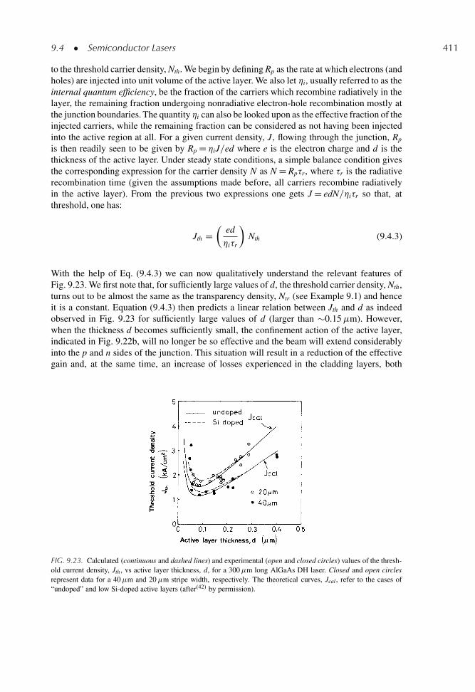
9.4 � Semiconductor Lasers 411
to the threshold carrier density, Nth. We begin by defining Rp as the rate at which electrons (andholes) are injected into unit volume of the active layer. We also let �i, usually referred to as theinternal quantum efficiency, be the fraction of the carriers which recombine radiatively in thelayer, the remaining fraction undergoing nonradiative electron-hole recombination mostly atthe junction boundaries. The quantity �i can also be looked upon as the effective fraction of theinjected carriers, while the remaining fraction can be considered as not having been injectedinto the active region at all. For a given current density, J, flowing through the junction, Rp
is then readily seen to be given by Rp D �iJ=ed where e is the electron charge and d is thethickness of the active layer. Under steady state conditions, a simple balance condition givesthe corresponding expression for the carrier density N as N D Rp�r, where �r is the radiativerecombination time (given the assumptions made before, all carriers recombine radiativelyin the active layer). From the previous two expressions one gets J D edN=�i�r so that, atthreshold, one has:
Jth D�
ed
�i�r
�Nth (9.4.3)
With the help of Eq. (9.4.3) we can now qualitatively understand the relevant features ofFig. 9.23. We first note that, for sufficiently large values of d, the threshold carrier density, Nth,turns out to be almost the same as the transparency density, Ntr (see Example 9.1) and henceit is a constant. Equation (9.4.3) then predicts a linear relation between Jth and d as indeedobserved in Fig. 9.23 for sufficiently large values of d (larger than �0.15�m). However,when the thickness d becomes sufficiently small, the confinement action of the active layer,indicated in Fig. 9.22b, will no longer be so effective and the beam will extend considerablyinto the p and n sides of the junction. This situation will result in a reduction of the effectivegain and, at the same time, an increase of losses experienced in the cladding layers, both
FIG. 9.23. Calculated (continuous and dashed lines) and experimental (open and closed circles) values of the thresh-old current density, Jth , vs active layer thickness, d, for a 300�m long AlGaAs DH laser. Closed and open circlesrepresent data for a 40�m and 20�m stripe width, respectively. The theoretical curves, Jcal , refer to the cases of“undoped” and low Si-doped active layers (after.42/ by permission).
412 9 � Solid-State, Dye, and Semiconductor Lasers
of which effects lead to a strongly increased Nth. So, at sufficiently small values of d, Jth isexpected to increase as d is decreased.
Example 9.1. Carrier and current densities at threshold for a DH GaAs laser Since the laser field isspace-dependent, the threshold condition must be derived, as in previous examples (see e.g., Sect. 6.3.4.),by setting the condition that the spatially averaged gain must equal the spatially averaged losses. Thus, ingeneral terms, we write
<g>L D <˛a>L C<˛n>L C<˛p>L C �m (9.4.4)
where L is the length of the active medium, g is the gain coefficient, ˛a is the scattering loss of the activelayer, ˛n and ˛p are the losses in the n and p sides of the cladding, respectively, and �m is the mirror loss.The average values appearing in Eq. (9.4.4) are to be taken over the field intensity distribution, so that, forexample, the average gain is given by
<g> DR
a gjUj2dVRc jUj2dV
(9.4.5)
where U.x, y, z/ is the field distribution within the laser cavity, the integral of the numerator is taken overthe volume of the active medium and the integral of the denominator is taken over the whole volumeof the cavity. The quantities <g> and <g>L are usually referred to as the modal gain coefficient andthe modal gain, respectively. Similar expressions hold for the average values appearing in the right handside of Eq. (9.4.4). For simplicity, we assume that ˛n Š˛p D ˛ and we neglect the spatial variation of thecavity field along the longitudinal z-coordinate (as produced by e.g. a standing wave pattern) and alongthe coordinate parallel to the junction. Then Eq. (9.4.4), with the help of Eq. (9.4.5) and the correspondingexpressions for <˛a> and <˛p>, readily gives
g� D ˛a� C ˛.1 � � /C Œln.1=R/=L� (9.4.6)
where R is the power reflectivity of the two end mirrors (assumed to be equal for the two mirrors) and
� D
Cd=2R�d=2
jUj2dx
C1R�1
jUj2dx
(9.4.7)
where x is the coordinate along the direction orthogonal to the junction. The quantity � represents thefraction of the beam power which is actually in the active layer and is usually referred to as the beamconfinement factor. According to the discussion in Sect. 3.2.5, we can now approximate g as g D�
.N � Ntr/ where � is the differential gain coefficient and Ntr is the carrier density at transparency. Ifwe now further assume, for simplicity, ˛a D ˛, then Eq. (9.4.6) simplifies to
�� .Nth � Ntr/ D ˛ C Œln.1=R/=L� D �=L (9.4.8)
where Nth is the threshold carrier density and � D ˛L C ln.1=R/ is the total loss per pass. From Eq. (9.4.8)we finally get the desired expression for the threshold carrier density as
Nth D .�=�L� /C Ntr (9.4.9)
9.4 � Semiconductor Lasers 413
To proceed with the calculation, we now need to evaluate the confinement factor � . A fairly accurate andsimple expression turns out to be given by given by.43/
� Š D2=.2 C D2/ (9.4.10)
where
D D 2 .n21 � n2
2/1=2d=� (9.4.11)
is the normalized thickness of the active layer (we recall that n1 and n2 are the refractive indices of theactive medium and cladding layers, respectively). If we now take n1 D 3.6, n2 D 3.4, and �D 850 nm (asappropriate for a GaAs laser) and we make the calculation for d D 0.1�m, we obtain D Š 0.875 and hence� Š 0.28. To obtain a numerical estimate of the corresponding value of Nth, we take the reflectivity of thetwo end faces equal to that of the uncoated surfaces .R Š 32%/, and assume a loss coefficient ˛Š 10 cm�1
and a cavity length of L D 300�m. We obtain � D ln.1=R/C ˛L Š 1.44. If we now take (see Table 3.1)� D 1.5 � 10�16 cm2 and Ntr D 2 � 1018 carriers=cm3, we obtain from Eq. (9.4.9)
Nth D .1.14 C 2/ � 1018 carriers/cm3 (9.4.12)
where, for convenience, the numerical values of the two terms appearing in the right hand side ofEq. (9.4.9) have been left separated. Equation (9.4.12) thus shows that, in this case, the first term, i.e.,the carrier density needed to overcome cavity losses, is comparable to Ntr.
The threshold current density is now readily obtained by substituting Eq. (9.4.9) in Eq. (9.4.3). We get
Jth D�
ed
�i�r
� h� �
�L�
�C Ntr
i(9.4.13)
We have seen that, for sufficiently large values of d, Ntr is the dominant term in the square bracket ofEq. (9.4.13). In this case Jth is expected to be proportional to d, as indeed shown in Fig. 9.23 for dlarger than �0.15�m, and most of the threshold pump current is just used to reach the semiconductortransparency condition. When d becomes very small, however, the confinement factor also becomes verysmall [according to Eq. (9.4.10), for very small values of d, one has � / d2/, the first term in thebrackets eventually dominates and Jth reaches a point where it increases with decreasing d. To get anumerical evaluation of Jth from Eq. (9.4.13), we assume d D 0.1�m, we take �i Š 1, �r D 4 ns and usethe previously calculated value of Nth. We obtain Jth Š 103 A=cm2 in reasonable agreement with the resultsof Fig. 9.23.
9.4.4. Quantum Well Lasers.44/
If the thickness of the active layer of a DH laser is greatly reduced to a pointwhere the dimension is comparable to the de-Broglie wavelength .�Š h=p/, where p isthe electron momentum a quantum well, QW, double heterostructure laser is produced.Such lasers exploit the more favorable optical properties of a QW or of a multiple
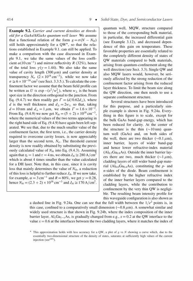
414 9 � Solid-State, Dye, and Semiconductor Lasers
Example 9.2. Carrier and current densities at thresh-old for a GaAs/AlGaAs quantum well laser We assumethat a functional relation of the form g D�.N � Nth/
still holds approximately for a QW�, so that the rela-tions established in Example 9.1. can still be applied. Tomake a comparison with the case discussed in Exam-ple 9.1, we take the same values of the loss coeffi-cient ˛.10 cm�1) and mirror reflectivity R (32%), henceof the total loss �.� D 1.44/. We also take the samevalue of cavity length .300�m/ and carrier density attransparency Ntr .2 � 1018 cm�3/, while we now take� Š 6 � 10�16 cm2 (see Sect. 3.3.5.). To calculate the con-finement factor we assume that the beam field profile canbe written as U / exp �.x2=w2?/, where w? is the beamspot size in the direction orthogonal to the junction. FromEq. (9.4.7) we then readily get � D .d=0.62d?/, whered is the well thickness and d? D 2w? so that, takingd D 10 nm and d? D 1�m, we obtain � D 1.6 � 10�2.From Eq. (9.4.9) we now get Nth D .5 C 2/� 1018 cm�3,where the numerical values of the two terms appearing inthe right hand side of Eq. (9.4.9) have again been left sep-arated. We see that, due to the much smaller value of theconfinement factor, the first term, i.e., the carrier densityrequired to overcome cavity losses, is now appreciablylarger than the second term, Ntr . The threshold currentdensity is now readily obtained by substituting the previ-ously calculated value of Nth into Eq. (9.4.3). Assumingagain that �i D 1 and � D 4 ns, we obtain Jth Š 280 A=cm2
which is about 4 times smaller than the value calculatedfor a DH laser. Note that, in this case, since it is cavityloss that mainly determines the value of Nth, a reductionof this loss is helpful to further reduce Jth. If we now take,for example, ˛D 3 cm�1 and R D 80%, we get � D 0.28,hence Nth D .2.3 C 2/� 1018 cm�3 and Jth Š 170 A=cm2.
quantum well, MQW, structure comparedto those of the corresponding bulk material,in particular, the increased differential gain(see Example 3.12), and decreased depen-dence of this gain on temperature. Thesefavorable properties are essentially related tothe completely different density of states ofQW materials compared to bulk materials,arising from quantum-confinement along thewell direction (see Sect. 3.3). Single QW andalso MQW lasers would, however, be seri-ously affected by the strong reduction of theconfinement factor arising from the reducedlayer thickness. To limit the beam size alongthe QW direction, one then needs to use aseparate confinement structure.
Several structures have been introducedfor this purpose, and a particularly sim-ple example is shown in Fig. 9.24a. Every-thing in this figure is to scale, except forthe bulk GaAs band-gap energy, which hasbeen reduced for clarity. At the center ofthe structure is the thin .�10 nm/ quan-tum well (GaAs) and, on both sides ofthe well, there are two thicker .�0.1�m/,inner barrier, layers of wider band-gapand hence lower refractive-index material.Al0.2Ga0.8As/. Outside the inner barrier lay-ers there are two, much thicker .�1�m/,cladding layers of still wider band-gap mate-rial .Al0.6Ga0.4As/, constituting the p- andn-sides of the diode. Beam confinement isestablished by the higher refractive indexof the inner barrier layers compared to thecladding layers, while the contribution toconfinement by the very thin QW is negligi-ble. The resulting beam intensity profile forthis waveguide configuration is also shown as
a dashed line in Fig. 9.24a. One can see that the full width between the 1=e2 points is, inthis case, confined to a comparatively small dimension .�0.8�m/. A somewhat similar andwidely used structure is that shown in Fig. 9.24b, where the index composition of the innerbarrier layer, AlxGa1�xAs, is gradually changed from e.g., x D 0.2 at the QW interface to thevalue x D 0.6 at the interfaces between the two cladding layers, where it matches the index of
� This approximation holds with less accuracy for a QW, a plot of g vs N showing a curve which, due to theessentially two-dimensional structure of the density of states, saturates at sufficiently high values of the currentinjection (see.45/).
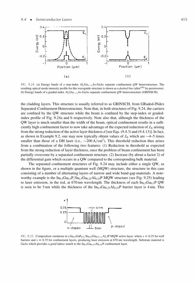
9.4 � Semiconductor Lasers 415
FIG. 9.24. (a) Energy bands of a step-index AlxGa1�xAs-GaAs separate confinement QW heterostructure. Theresulting optical mode intensity profile for this waveguide structure is shown as a dashed line (after.46/ by permission).(b) Energy bands of a graded-index AlxGa1�xAs-GaAs separate confinement QW heterostructure (GRINSCH).
the cladding layers. This structure is usually referred to as GRINSCH, from GRaded-INdexSeparated-Confinement Heterostructure. Note that, in both structures of Fig. 9.24, the carriersare confined by the QW structure while the beam is confined by the step-index or graded-index profile of Fig. 9.24a and b respectively. Note also that, although the thickness of theQW layer is much smaller than the width of the beam, optical confinement results in a suffi-ciently high confinement factor to now take advantage of the expected reduction of Jth arisingfrom the strong reduction of the active layer thickness d [see Eqs. (9.4.3) and (9.4.13)]. In fact,as shown in Example 9.2, one may now typically obtain values of Jth which are �4–5 timessmaller than those of a DH laser (i.e., �200 A=cm2). This threshold reduction thus arisesfrom a combination of the following two features: (1) Reduction in threshold as expectedfrom the strong reduction of layer thickness, once the problem of beam confinement has beenpartially overcome by a separated confinement structure. (2) Increase (by about a factor 2) ofthe differential gain which occurs in a QW compared to the corresponding bulk material.
The separated confinement structures of Fig. 9.24 may include either a single QW, asshown in the figure, or a multiple quantum well (MQW) structure, the structure in this caseconsisting of a number of alternating layers of narrow and wide band-gap materials. A note-worthy example is the In0.5Ga0.5P=In0.5Ga0.25Al0.25P MQW structure (see Fig. 9.25) leadingto laser emission, in the red, at 670 nm wavelength. The thickness of each In0.5Ga0.5P QWis seen to be 5 nm while the thickness of the In0.5Ga0.25Al0.25P barrier layer is 4 nm. This
FIG. 9.25. Composition variations in a In0.5GaP0.5=In0.5.Ga0.5�xAlx/P MQW active layer, where x D 0.25 for wellbarriers and x D 0.35 for confinement layers, producing laser emission at 670 nm wavelength. Substrate material isGaAs which provides a good lattice match to the In0.5Ga0.15Al0.35P confinement layer.
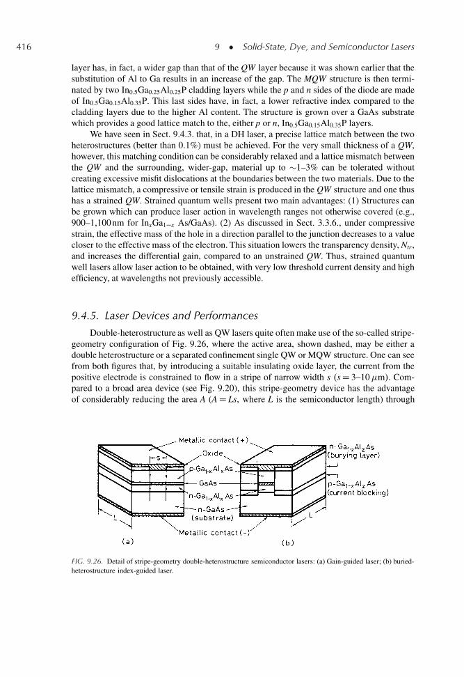
416 9 � Solid-State, Dye, and Semiconductor Lasers
layer has, in fact, a wider gap than that of the QW layer because it was shown earlier that thesubstitution of Al to Ga results in an increase of the gap. The MQW structure is then termi-nated by two In0.5Ga0.25Al0.25P cladding layers while the p and n sides of the diode are madeof In0.5Ga0.15Al0.35P. This last sides have, in fact, a lower refractive index compared to thecladding layers due to the higher Al content. The structure is grown over a GaAs substratewhich provides a good lattice match to the, either p or n, In0.5Ga0.15Al0.35P layers.
We have seen in Sect. 9.4.3. that, in a DH laser, a precise lattice match between the twoheterostructures (better than 0.1%) must be achieved. For the very small thickness of a QW,however, this matching condition can be considerably relaxed and a lattice mismatch betweenthe QW and the surrounding, wider-gap, material up to �1–3% can be tolerated withoutcreating excessive misfit dislocations at the boundaries between the two materials. Due to thelattice mismatch, a compressive or tensile strain is produced in the QW structure and one thushas a strained QW. Strained quantum wells present two main advantages: (1) Structures canbe grown which can produce laser action in wavelength ranges not otherwise covered (e.g.,900–1,100 nm for InxGa1�x As/GaAs). (2) As discussed in Sect. 3.3.6., under compressivestrain, the effective mass of the hole in a direction parallel to the junction decreases to a valuecloser to the effective mass of the electron. This situation lowers the transparency density, Ntr ,and increases the differential gain, compared to an unstrained QW. Thus, strained quantumwell lasers allow laser action to be obtained, with very low threshold current density and highefficiency, at wavelengths not previously accessible.
9.4.5. Laser Devices and Performances
Double-heterostructure as well as QW lasers quite often make use of the so-called stripe-geometry configuration of Fig. 9.26, where the active area, shown dashed, may be either adouble heterostructure or a separated confinement single QW or MQW structure. One can seefrom both figures that, by introducing a suitable insulating oxide layer, the current from thepositive electrode is constrained to flow in a stripe of narrow width s .s D 3–10�m/. Com-pared to a broad area device (see Fig. 9.20), this stripe-geometry device has the advantageof considerably reducing the area A (A D Ls, where L is the semiconductor length) through
FIG. 9.26. Detail of stripe-geometry double-heterostructure semiconductor lasers: (a) Gain-guided laser; (b) buried-heterostructure index-guided laser.
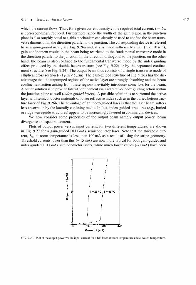
9.4 � Semiconductor Lasers 417
which the current flows. Thus, for a given current density J, the required total current, I D JA,is correspondingly reduced. Furthermore, since the width of the gain region in the junctionplane is also roughly equal to s, this mechanism can already be used to confine the beam trans-verse dimension in the direction parallel to the junction. The corresponding device is referredto as a gain-guided laser, see Fig. 9.26a and, if s is made sufficiently small .s < 10�m/,gain confinement results in the beam being restricted to the fundamental transverse mode inthe direction parallel to the junction. In the direction orthogonal to the junction, on the otherhand, the beam is also confined to the fundamental transverse mode by the index guidingeffect produced by the double heterostrusture (see Fig. 9.22) or by the separated confine-ment structure (see Fig. 9.24). The output beam thus consists of a single transverse mode ofelliptical cross section .�1�m � 5�m/. The gain-guided structure of Fig. 9.26a has the dis-advantage that the unpumped regions of the active layer are strongly absorbing and the beamconfinement action arising from these regions inevitably introduces some loss for the beam.A better solution is to provide lateral confinement via a refractive-index guiding action withinthe junction plane as well (index-guided lasers). A possible solution is to surround the activelayer with semiconductor materials of lower refractive index such as in the buried heterostruc-ture laser of Fig. 9.26b. The advantage of an index-guided laser is that the laser beam suffersless absorption by the laterally confining media. In fact, index-guided structures (e.g., buriedor ridge waveguide structures) appear to be increasingly favored in commercial devices.
We now consider some properties of the output beam namely output power, beamdivergence and spectral content.
Plots of output power versus input current, for two different temperatures, are shownin Fig. 9.27 for a gain-guided DH GaAs semiconductor laser. Note that the threshold cur-rent, Ith, at room temperature is less than 100 mA as a result of using the stripe geometry.Threshold currents lower than this .�15 mA/ are now more typical for both gain-guided andindex-guided DH GaAs semiconductor lasers, while much lower values .�1 mA/ have been
FIG. 9.27. Plot of the output power vs the input current for a DH laser at room temperature and elevated temperature.
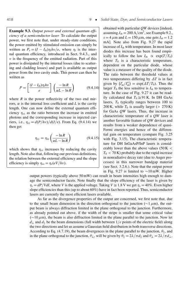
418 9 � Solid-State, Dye, and Semiconductor Lasers
Example 9.3. Output power and external quantum effi-ciency of a semiconductor laser To calculate the outputpower, we first note that, under steady-state conditions,the power emitted by stimulated emission can simply bewritten as Pe D .I � Ith/�ih�=e, where �i is the inter-nal quantum efficiency, introduced in Sect. 9.4.3., and� is the frequency of the emitted radiation. Part of thispower is dissipated by the internal losses (due to scatter-ing and cladding losses) and part is available as outputpower from the two cavity ends. This power can then bewritten as
P D�.I � Ith/�ih�
e
� � � ln R
˛L � ln R
�(9.4.14)
where R is the power reflectivity of the two end mir-rors, ˛ is the internal loss coefficient and L is the cavitylength. One can now define the external quantum effi-ciency �ex as the ratio between the increase in emittedphotons and the corresponding increase in injected car-riers, i.e., �ex D d.P=h�/=d.I=e/. From Eq. (9.4.14) wethen get
�ex D �in
� � ln R
˛L � ln R
�(9.4.15)
which shows that �ex increases by reducing the cavitylength. Note also that, following our previous definitions,the relation between the external efficiency and the slopeefficiency is simply �ex D �s.eV=h�/.
obtained with particular QW devices [indeed,assuming Jth D 200 A=cm2, see Example 9.2.,s D 4�m and L D 150�m, one gets Ith D 1.2mA]. Note also from Fig. 9.27 the rapidincrease of Ith with temperature. In most laserdiodes this increase has been found empir-ically to follow the law Ith / exp.T=T0/
where T0 is a characteristic temperature,dependent on the particular diode, whosevalue is a measure of the quality of the diode.The ratio between the threshold values attwo temperatures differing by T is in factgiven by
I0th=I00
th
� D exp.T=T0/. Thus thelarger T0 the less sensitive is Ith to tempera-ture. In the case of Fig. 9.27 it can be read-ily calculated that T0 Š 91 K. In DH GaAslasers, T0 typically ranges between 100 to200 K, while T0 is usually larger .> 270 K/for GaAs QW lasers. Thus, the increase incharacteristic temperature of a QW laser isanother favorable feature of QW devices andresults from a weaker dependence of quasi-Fermi energies and hence of the differen-tial gain on temperature (compare Fig. 3.25with Fig. 3.15). The characteristic tempera-ture for DH InGaAsP/InP lasers is consid-erably lower than the above values .50 K <
T0 < 70 K/ probably due to the rapid increasein nonradiative decay rate (due to Auger pro-cesses) in this narrower bandgap material(see Sect. 3.2.6.). Note that the output powerin Fig. 9.27 is limited to �10 mW. Higher
output powers (typically above 50 mW) can result in beam intensities high enough to dam-age the semiconductor facets. Note finally that the slope efficiency of the laser is given by�s D dP=VdI, where V is the applied voltage. Taking V Š 1.8 V we get �s D 40%. Even higherslope efficiencies than this (up to about 60%) have in fact been reported. Thus, semiconductorlasers are currently the most efficient lasers available.
As far as the divergence properties of the output are concerned, we first note that, dueto the small beam dimension in the direction orthogonal to the junction .�1�m/, the out-put beam is always diffraction limited in the plane orthogonal to the junction. Furthermore,as already pointed out above, if the width of the stripe is smaller that some critical value.�10�m/, the beam is also diffraction limited in the plane parallel to the junction. Now letd? and djj be the beam dimensions (full width between 1=e points of the electric field) alongthe two directions and let us assume a Gaussian field distribution in both transverse directions.According to Eq. (4.7.19), the beam divergences in the plane parallel to the junction, jj, andin the plane orthogonal to the junction, ?, will be given by jj D 2�= djj and ? D 2�= d?,
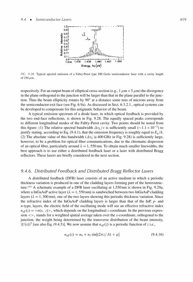
9.4 � Semiconductor Lasers 419
FIG. 9.28. Typical spectral emission of a Fabry-Perot type DH GaAs semiconductor laser with a cavity lengthof 250�m.
respectively. For an output beam of elliptical cross-section (e.g., 1�m � 5�m) the divergencein the plane orthogonal to the junction will be larger than that in the plane parallel to the junc-tion. Thus the beam ellipticity rotates by 90ı at a distance some tens of microns away fromthe semiconductor exit face (see Fig. 6.9a). As discussed in Sect. 6.3.2.1., optical systems canbe developed to compensate for this astigmatic behavior of the beam.
A typical emission spectrum of a diode laser, in which optical feedback is provided bythe two end-face reflections, is shown in Fig. 9.28. The equally spaced peaks correspondsto different longitudinal modes of the Fabry-Perot cavity. Two points should be noted fromthis figure: (1) The relative spectral bandwidth �L=� is sufficiently small .�1.1 � 10�3/ tojustify stating, according to Eq. (9.4.1), that the emission frequency is roughly equal to Eg=h.(2) The absolute value of this bandwidth (�L Š 400 GHz in Fig. 9.28) is sufficiently large,however, to be a problem for optical fiber communications, due to the chromatic dispersionof an optical fiber, particularly around �D 1, 550 nm. To obtain much smaller linewidths, thebest approach is to use either a distributed feedback laser or a laser with distributed Braggreflectors. These lasers are briefly considered in the next section.
9.4.6. Distributed Feedback and Distributed Bragg Reflector Lasers
A distributed feedback (DFB) laser consists of an active medium in which a periodicthickness variation is produced in one of the cladding layers forming part of the heterostruc-ture..47/ A schematic example of a DFB laser oscillating at 1,550 nm is shown in Fig. 9.29a,where a InGaAsP active layer .�D 1, 550 nm/ is sandwiched between two InGaAsP claddinglayers .�D 1, 300 nm/, one of the two layers showing this periodic thickness variation. Sincethe refractive index of the InGaAsP cladding layers is larger than that of the InP, p- andn-type, layers, the electric field of the oscillating mode will see an effective refractive indexneff .z/D<n.x, z/>x which depends on the longitudinal z-coordinate. In the previous expres-sion <>x stands for a weighted spatial average taken over the x-coordinate, orthogonal to thejunction, the weight being determined by the transverse distribution of the beam intensity,jU.x/j2 [see also Eq. (9.4.5)]. We now assume that neff .z/ is a periodic function of z i.e.,
neff .z/ D n0 C n1 sinŒ.2 z=�/C '� (9.4.16)
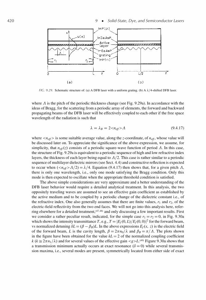
420 9 � Solid-State, Dye, and Semiconductor Lasers
FIG. 9.29. Schematic structure of: (a) A DFB laser with a uniform grating. (b) A �=4-shifted DFB laser.
where� is the pitch of the periodic thickness change (see Fig. 9.29a). In accordance with theideas of Bragg, for the scattering from a periodic array of elements, the forward and backwardpropagating beams of the DFB laser will be effectively coupled to each other if the free spacewavelength of the radiation is such that
� D �B D 2<neff>� (9.4.17)
where<neff> is some suitable average value, along the z-coordinate, of neff , whose value willbe discussed later on. To appreciate the significance of the above expression, we assume, forsimplicity, that neff .z/ consists of a periodic square-wave function of period �. In this case,the structure of Fig. 9.29a is equivalent to a periodic sequence of high and low refractive indexlayers, the thickness of each layer being equal to�=2. This case is rather similar to a periodicsequence of multilayer dielectric mirrors (see Sect. 4.4) and constructive reflection is expectedto occur when .<neff>�=2/D�=4. Equation (9.4.17) then shows that, for a given pitch �,there is only one wavelength, i.e., only one mode satisfying the Bragg condition. Only thismode is then expected to oscillate when the appropriate threshold condition is satisfied.
The above simple considerations are very approximate and a better understanding of theDFB laser behavior would require a detailed analytical treatment. In this analysis, the twooppositely traveling waves are assumed to see an effective gain coefficient as established bythe active medium and to be coupled by a periodic change of the dielectric constant i.e., ofthe refractive index. One also generally assumes that there are finite values, r1 and r2, of theelectric-field reflectivity from the two end faces. We will not go into this analysis here, refer-ring elsewhere for a detailed treatment,.47,48/ and only discussing a few important results. Firstwe consider a rather peculiar result, indicated, for the simple case r1 D r2 D 0, in Fig. 9.30awhich shows the intensity transmittance T, e.g., T D jEf .0, L/=Ef .0, 0/j2 for the forward beam,vs normalized detuning ıL D .ˇ �ˇB/L. In the above expressions Ef .x, z/ is the electric fieldof the forward beam, L is the cavity length, ˇD 2 n0=� and ˇB D =�. The plots shownin the figure have been obtained for the value kL D 2 of the normalized coupling coefficientk .k Š 2 n1=�/ and for several values of the effective gain <g>L..49/ Figure 9.30a shows thata transmission minimum actually occurs at exact resonance .ıD 0/ while several transmis-sion maxima, i.e., several modes are present, symmetrically located from either side of exact
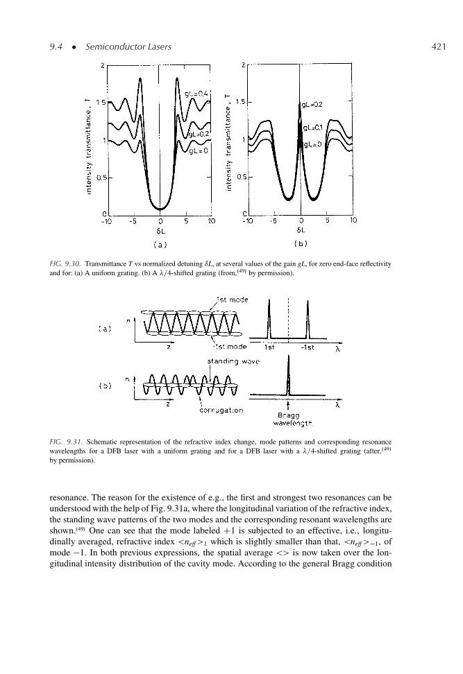
9.4 � Semiconductor Lasers 421
FIG. 9.30. Transmittance T vs normalized detuning ıL, at several values of the gain gL, for zero end-face reflectivityand for: (a) A uniform grating. (b) A �=4-shifted grating (from,.49/ by permission).
FIG. 9.31. Schematic representation of the refractive index change, mode patterns and corresponding resonancewavelengths for a DFB laser with a uniform grating and for a DFB laser with a �=4-shifted grating (after,.49/
by permission).
resonance. The reason for the existence of e.g., the first and strongest two resonances can beunderstood with the help of Fig. 9.31a, where the longitudinal variation of the refractive index,the standing wave patterns of the two modes and the corresponding resonant wavelengths areshown..49/ One can see that the mode labeled C1 is subjected to an effective, i.e., longitu-dinally averaged, refractive index <neff>1 which is slightly smaller than that, <neff>�1, ofmode �1. In both previous expressions, the spatial average <> is now taken over the lon-gitudinal intensity distribution of the cavity mode. According to the general Bragg condition
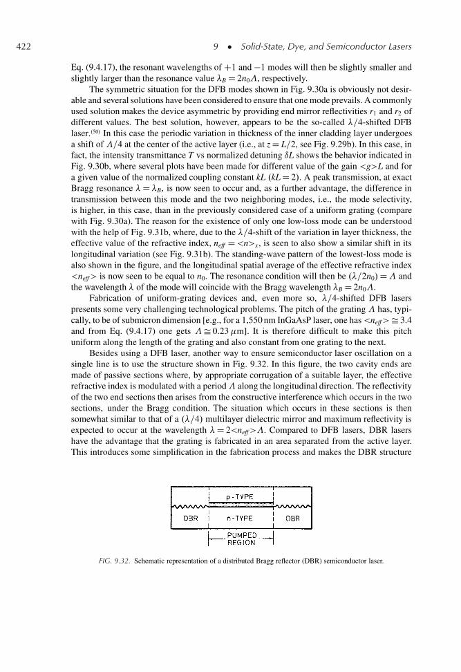
422 9 � Solid-State, Dye, and Semiconductor Lasers
Eq. (9.4.17), the resonant wavelengths of C1 and �1 modes will then be slightly smaller andslightly larger than the resonance value �B D 2n0�, respectively.
The symmetric situation for the DFB modes shown in Fig. 9.30a is obviously not desir-able and several solutions have been considered to ensure that one mode prevails. A commonlyused solution makes the device asymmetric by providing end mirror reflectivities r1 and r2 ofdifferent values. The best solution, however, appears to be the so-called �=4-shifted DFBlaser..50/ In this case the periodic variation in thickness of the inner cladding layer undergoesa shift of �=4 at the center of the active layer (i.e., at z D L=2, see Fig. 9.29b). In this case, infact, the intensity transmittance T vs normalized detuning ıL shows the behavior indicated inFig. 9.30b, where several plots have been made for different value of the gain <g>L and fora given value of the normalized coupling constant kL .kL D 2/. A peak transmission, at exactBragg resonance �D�B, is now seen to occur and, as a further advantage, the difference intransmission between this mode and the two neighboring modes, i.e., the mode selectivity,is higher, in this case, than in the previously considered case of a uniform grating (comparewith Fig. 9.30a). The reason for the existence of only one low-loss mode can be understoodwith the help of Fig. 9.31b, where, due to the �=4-shift of the variation in layer thickness, theeffective value of the refractive index, neff D<n>x, is seen to also show a similar shift in itslongitudinal variation (see Fig. 9.31b). The standing-wave pattern of the lowest-loss mode isalso shown in the figure, and the longitudinal spatial average of the effective refractive index<neff> is now seen to be equal to n0. The resonance condition will then be .�=2n0/D� andthe wavelength � of the mode will coincide with the Bragg wavelength �B D 2n0�.
Fabrication of uniform-grating devices and, even more so, �=4-shifted DFB laserspresents some very challenging technological problems. The pitch of the grating� has, typi-cally, to be of submicron dimension [e.g., for a 1,550 nm InGaAsP laser, one has<neff>Š 3.4and from Eq. (9.4.17) one gets �Š 0.23�m]. It is therefore difficult to make this pitchuniform along the length of the grating and also constant from one grating to the next.
Besides using a DFB laser, another way to ensure semiconductor laser oscillation on asingle line is to use the structure shown in Fig. 9.32. In this figure, the two cavity ends aremade of passive sections where, by appropriate corrugation of a suitable layer, the effectiverefractive index is modulated with a period� along the longitudinal direction. The reflectivityof the two end sections then arises from the constructive interference which occurs in the twosections, under the Bragg condition. The situation which occurs in these sections is thensomewhat similar to that of a .�=4/ multilayer dielectric mirror and maximum reflectivity isexpected to occur at the wavelength �D 2<neff>�. Compared to DFB lasers, DBR lasershave the advantage that the grating is fabricated in an area separated from the active layer.This introduces some simplification in the fabrication process and makes the DBR structure
FIG. 9.32. Schematic representation of a distributed Bragg reflector (DBR) semiconductor laser.
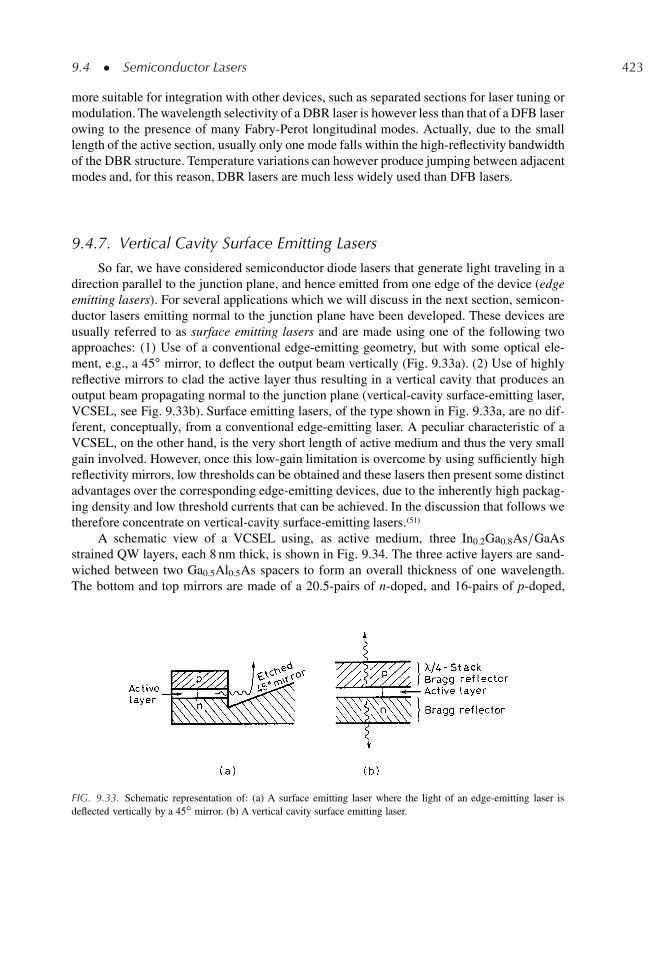
9.4 � Semiconductor Lasers 423
more suitable for integration with other devices, such as separated sections for laser tuning ormodulation. The wavelength selectivity of a DBR laser is however less than that of a DFB laserowing to the presence of many Fabry-Perot longitudinal modes. Actually, due to the smalllength of the active section, usually only one mode falls within the high-reflectivity bandwidthof the DBR structure. Temperature variations can however produce jumping between adjacentmodes and, for this reason, DBR lasers are much less widely used than DFB lasers.
9.4.7. Vertical Cavity Surface Emitting Lasers
So far, we have considered semiconductor diode lasers that generate light traveling in adirection parallel to the junction plane, and hence emitted from one edge of the device (edgeemitting lasers). For several applications which we will discuss in the next section, semicon-ductor lasers emitting normal to the junction plane have been developed. These devices areusually referred to as surface emitting lasers and are made using one of the following twoapproaches: (1) Use of a conventional edge-emitting geometry, but with some optical ele-ment, e.g., a 45ı mirror, to deflect the output beam vertically (Fig. 9.33a). (2) Use of highlyreflective mirrors to clad the active layer thus resulting in a vertical cavity that produces anoutput beam propagating normal to the junction plane (vertical-cavity surface-emitting laser,VCSEL, see Fig. 9.33b). Surface emitting lasers, of the type shown in Fig. 9.33a, are no dif-ferent, conceptually, from a conventional edge-emitting laser. A peculiar characteristic of aVCSEL, on the other hand, is the very short length of active medium and thus the very smallgain involved. However, once this low-gain limitation is overcome by using sufficiently highreflectivity mirrors, low thresholds can be obtained and these lasers then present some distinctadvantages over the corresponding edge-emitting devices, due to the inherently high packag-ing density and low threshold currents that can be achieved. In the discussion that follows wetherefore concentrate on vertical-cavity surface-emitting lasers..51/
A schematic view of a VCSEL using, as active medium, three In0.2Ga0.8As=GaAsstrained QW layers, each 8 nm thick, is shown in Fig. 9.34. The three active layers are sand-wiched between two Ga0.5Al0.5As spacers to form an overall thickness of one wavelength.The bottom and top mirrors are made of a 20.5-pairs of n-doped, and 16-pairs of p-doped,
FIG. 9.33. Schematic representation of: (a) A surface emitting laser where the light of an edge-emitting laser isdeflected vertically by a 45ı mirror. (b) A vertical cavity surface emitting laser.
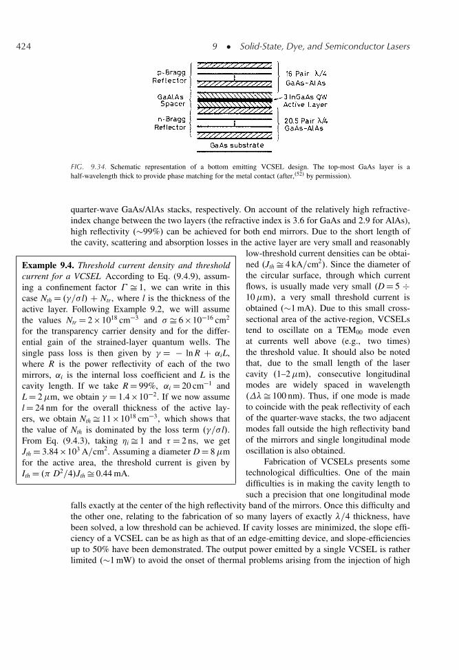
424 9 � Solid-State, Dye, and Semiconductor Lasers
FIG. 9.34. Schematic representation of a bottom emitting VCSEL design. The top-most GaAs layer is ahalf-wavelength thick to provide phase matching for the metal contact (after,.52/ by permission).
quarter-wave GaAs/AlAs stacks, respectively. On account of the relatively high refractive-index change between the two layers (the refractive index is 3.6 for GaAs and 2.9 for AlAs),high reflectivity .�99%/ can be achieved for both end mirrors. Due to the short length ofthe cavity, scattering and absorption losses in the active layer are very small and reasonably
Example 9.4. Threshold current density and thresholdcurrent for a VCSEL According to Eq. (9.4.9), assum-ing a confinement factor � Š 1, we can write in thiscase Nth D .�=� l/ C Ntr, where l is the thickness of theactive layer. Following Example 9.2, we will assumethe values Ntr D 2 � 1018 cm�3 and � Š 6 � 10�16 cm2
for the transparency carrier density and for the differ-ential gain of the strained-layer quantum wells. Thesingle pass loss is then given by � D � ln R C ˛iL,where R is the power reflectivity of each of the twomirrors, ˛i is the internal loss coefficient and L is thecavity length. If we take R D 99%, ˛i D 20 cm�1 andL D 2�m, we obtain � D 1.4 � 10�2. If we now assumel D 24 nm for the overall thickness of the active lay-ers, we obtain Nth Š 11 � 1018 cm�3, which shows thatthe value of Nth is dominated by the loss term .�=� l/.From Eq. (9.4.3), taking �i Š 1 and � D 2 ns, we getJth D 3.84 � 103 A=cm2. Assuming a diameter D D 8�mfor the active area, the threshold current is given byIth D . D2=4/Jth Š 0.44 mA.
low-threshold current densities can be obtai-ned .Jth Š 4 kA=cm2/. Since the diameter ofthe circular surface, through which currentflows, is usually made very small .D D 5 �10�m/, a very small threshold current isobtained .�1 mA/. Due to this small cross-sectional area of the active-region, VCSELstend to oscillate on a TEM00 mode evenat currents well above (e.g., two times)the threshold value. It should also be notedthat, due to the small length of the lasercavity .1–2�m/, consecutive longitudinalmodes are widely spaced in wavelength.�Š 100 nm/. Thus, if one mode is madeto coincide with the peak reflectivity of eachof the quarter-wave stacks, the two adjacentmodes fall outside the high reflectivity bandof the mirrors and single longitudinal modeoscillation is also obtained.
Fabrication of VCSELs presents sometechnological difficulties. One of the maindifficulties is in making the cavity length tosuch a precision that one longitudinal mode
falls exactly at the center of the high reflectivity band of the mirrors. Once this difficulty andthe other one, relating to the fabrication of so many layers of exactly �=4 thickness, havebeen solved, a low threshold can be achieved. If cavity losses are minimized, the slope effi-ciency of a VCSEL can be as high as that of an edge-emitting device, and slope-efficienciesup to 50% have been demonstrated. The output power emitted by a single VCSEL is ratherlimited .�1 mW/ to avoid the onset of thermal problems arising from the injection of high
9.4 � Semiconductor Lasers 425
pump powers into such a small volume of active layer. Arrays of e.g., 8 � 8, independentlyaddressable, lasers as well as matrix-addressable arrays have been made.
9.4.8. Applications of Semiconductor Lasers
Semiconductor lasers lend themselves to a large variety of both low-power and high-power applications, some of which will be briefly reviewed here. We first refer to Table 9.7where some characteristics of the most common DH or QW lasers are presented. Sinceall the structures shown are grown on either a GaAs or InP substrate, the laser materialis characterized by the active layer-substrate combination. In each case, the laser wave-length is largely determined by the composition index of the active layer and, for a QWlaser, also by the thickness of this layer. Most recent lasers use separated-confinement(e.g., GRINSCH) QW and MQW layers in a gain-guiding or, more often, index guidingconfiguration.
In the AlxGa1�xAs=AlyGa1�yAs laser structures, the composition index y of the claddinglayers must be larger than that, x, of the active layer. Depending on the value of this last com-position index, the emission wavelength usually ranges between 720 and 850 nm. Low-power.P D 5–20 mW/, single-stripe devices are widely used in Compact-Disk (CD) players andlaser printers. Higher power single-stripe lasers, laser arrays, laser bars and stacks of laserbars (Figs. 6.9 and 6.10) are used to pump solid-state lasers such as Nd (pump wavelength�p Š 800 nm), Tm:Ho .�p Š 790 nm/ and Cr:LISAF .�p Š 670 nm/. Some of these laser sys-tems and the corresponding fields of applications have been discussed in Sect. 9.2 of thischapter as well as in previous chapters.
In the In1�xGaxAsyP1�y/InP lasers, lattice matching is achieved by letting y Š 2.2 x andthe oscillation wavelength covers the so-called second (centered at �D 1, 310 nm, which cor-responds to x D 0.27) and third (�D 1, 550 nm center wavelength, corresponding to x D 0.42)transmission windows of optical fibers. Thus, these lasers find their widest use in opticalcommunications. Most recent optical communication systems use lasers around 1,550 nmwavelength. Due to the relatively large group-delay dispersion of optical fibers around thiswavelength, narrow-linewidth .�L<10 MHz/ DFB lasers are now widely used. With these
TABLE 9.7. Some characteristic parameters of the most important semiconductor laserdiodes
Material/Substrate AlGaAs/GaAs InGaAsP/InP InGaAs/GaAs InGaAlP/GaAs
Wavelength[nm]
720–850 1,200–1,650 900–1,100 630–700
Internal loss 4–15 5–10 2–10 �10Œcm�1�
Thresholdcurrent densityJth ŒA=cm2�
80–700 200–1,500 50–400 200–3,000
CharacteristicTemperatureT0 ŒK�
120–200 50–70 100–200 60–100
426 9 � Solid-State, Dye, and Semiconductor Lasers
lasers, modulation rates up to a few Gbits/s have been demonstrated by direct modula-tion of the diode current. Even higher modulation rates (up to a few tens of Gbits/s) havealso been demonstrated using external modulators such as LiNbO3 waveguide modulators.For communication systems operating at even larger communication bit-rates (from a fewhundreds Gbit/s up to the Tbit/s range) Wavelength-Division-Multiplexing (WDM) systemshave increasingly been used. For this application, many DFB lasers tuned at distinct wave-lengths in the low transparency region (spanning �13 THz) around 1,550 nm wavelengthare used. Systems based on WDM thus allow exceptionally high bit rate capacity to beachieved.
In1�xGaxAs=GaAs strained-layer QW lasers allow oscillation to be obtained over a widerange (900–1,100nm) at previously inaccessible wavelengths. Lasers with emission around980 nm wavelength .x D 0.8/ are of particular interest as pumps for Er-doped fiber amplifiersand lasers as well as for pumping Yb:Er:glass and Yb:YAG lasers. For these applications,output powers up to �100 mW are available in a diffraction-limited beam (of 1 � 4�m area)and up to �1 W from a broader area .1 � 30�m/ device. To obtain higher output pow-ers (�40 W or even larger), diode laser arrays and laser bars are also available. Given thefavorable laser properties of strained-layer QW structures, vertical-cavity surface-emittinglasers based on In1�xGaxAS=GaAs structures have been particularly actively developed. Theypromise to offer interesting solutions for optical interconnects, optical communications, andoptical signal processing.
InGaAlP/GaAs lasers are particularly interesting since they emit radiation in the visi-ble, red, region of the e.m. spectrum..53/ The In0.5Ga0.5P=In0.5.Ga0.5�xAlx/P QW or MQWstructure (where x D 0.25 for the well barriers and x D 0.35 for the confinement layers, seeFig. 9.25) oscillating at 670 nm wavelength has been particularly developed. These lasers arecommercially available with sufficiently high power (up to �10 mW) and long lifetime to beused for CD players or as substitutes for red-emitting He-Ne lasers for applications such asbar-code scanners and general alignment uses.
The development of semiconductor lasers is by no means limited to the laser cat-egories shown in Table 9.7. On the short wavelength side (blue-green region) the mostinteresting category now appears to be the III-V nitride-based diode-lasers, e.g., theIn0.2Ga0.8N=In0.05Ga0.95N MQW structure oscillating in the blue (417 nm)..54/ In the samewavelength region, wide-gap II-VI lasers such as ZnCdSe/ZnSSe QW lasers have also beendemonstrated. After a number of years of intense development, however, these lasers arestill suffering from a few technological limitations with particular problems of rather limitedoperating lifetime .�100 h/. Although nitride-lasers also present similar lifetime problems(less than 100 h), their recent development and the rapid progress which is occurring indi-cate nitride-based diode-lasers as the best candidates for blue-green semiconductor emitters.Potentially, blue-green lasers are of strong interest for e.g. a new generation of CD playerswhere, due to the shorter wavelength, substantially higher bit densities could be achieved onthe CD. On the long wavelength side, on the other hand, we just mention the IV–VI com-pounds such as the Pb and Sn salts (e.g., PbSSe, PbSnTe, and PbSnSe), oscillating in themiddle-far infrared .4–29�m/. All these lasers, however, need to operate at cryogenic tem-peratures .T<100 K/ to avoid problems such as the increased free-carrier absorption and theincreased rate of non-radiative decay arising from the much narrower band-gaps. Thus, due tothis cryogenic requirement, these lasers have found only a limited use (e.g., for spectroscopy).It should be noted, however, that the recent invention of a quantum-cascade laser promisesefficient mid-IR sources without the need for cryogenic temperatures..33/
Problems 427
9.5. CONCLUSIONS
In this chapter, a few of the most notable solid-state, dye and semiconductor lasers havebeen considered. These lasers use high-density active media and thus share a few commonfeatures. A first feature is that they generally show wide and strong absorption band(s) whichindicates that they are generally suitable for optical pumping, this type of pumping being infact always used for solid-state and dye lasers and sometimes also used for semiconductorlasers. The high values of absorption coefficient allow for lasers with dimensions down toa few microns (microlasers). A second relevant feature is that these media generally showwide fluorescence, and hence wide gain bandwidths. On the one hand, this offers tunabil-ity over wide (a few to several nm) bandwidths. On the other hand, this also implies thatvery short pulse durations (femtoseconds) can be obtained in mode-locked operation. A thirdrelevant feature is that the optical-to-optical laser efficiency, for solid-state and dye media,and electrical to optical efficiency, for semiconductors, is generally quite large. It should alsobe noted that laser pumping involving combination of these three categories of lasers hasbeen used increasingly (e.g., diode-pumped solid-state lasers or solid-state-laser pumped dyelasers) thus allowing compact and efficient lasers to be realized. Thus, as a conclusion, high-density laser media appear to present some of the best solutions to requirements for laserradiation in the visible-to-near-infrared range, even at high power levels.
PROBLEMS
9.1. Make up a diagram in which the tuning ranges of all the tunable solid-state lasers considered inthis chapter are plotted vs oscillation wavelength.
9.2. For pollution monitoring, a tunable laser oscillating around 720 nm wavelength is needed. Whichkind of solid-state laser would you use?
9.3. For biomedical photo-coagulation purposes, using an endoscopic apparatus, a cw laser with powerexceeding 50 W needs to be used. Which laser would you use?
9.4. For material working applications, a laser with an average power of 2 kW, to be transmittedthrough a �1 mm diameter optical fiber, is needed. Which laser would you use?
9.5. Consider a 6 mm diameter, 10 cm long Nd:phosphate glass laser rod. Using data from Table 9.3and the results discussed in Sect. 2.9.2., calculate the maximum inversion and the correspondingmaximum value of stored energy which are allowed if the onset of amplified spontaneous emis-sion is to be avoided. Compare the results obtained with those for a Nd:YAG rod of the samedimensions.
9.6. With reference to the energy level diagram of alexandrite shown in Fig. 9.8, assume that the4T2 and the 2E states are strongly coupled and take �T D 1.5 ms and �E D 6.6�s as the lifetimesof the two states. Knowing that the degeneracy of the two states is the same .g D 4/, calculatethe effective lifetime of the 4T2 state at T D 300 K and T D 400 K. Knowing that the true cross-section for the 4T2 ! 4A2 transition is � Š 4 � 10�19 cm2, calculate then the effective value ofthe cross section at the two temperatures. Using these results, consider whether the laser thresholdis expected to increase or decrease when the crystal temperature is raised from 300 to 400 K.
428 9 � Solid-State, Dye, and Semiconductor Lasers
9.7. Consider a Cr:LISAF laser longitudinally pumped, at 647.1 nm wavelength, by a Kr ion laser.Assume the linearly polarized beam of the laser to be sent along the c-axis of the LISAF andassume an active medium with 1 at. % Cr3C concentration and a length l D 4 mm. Also assumeboth pump and mode spot sizes to be matched to a value of 60 μm, the output coupling trans-mission to be 1%, and the internal loss per pass to be 1%. Using data from Fig. 9.11 and fromTable 9.5 and neglecting both ground-state and excited-state absorption, calculate the expectedthreshold pump power.
9.8. With reference to the previous problem, how would the expression for the threshold pump power,given by Eq. (6.3.19), need to be modified if ground state absorption, characterized by a loss perpass �a, and excited-state absorption, characterized by an excited-state absorption cross-section�ESA, were taken into account? Compare the result with that given in..25/
9.9. Derive an expression for the threshold pump power of a longitudinally pumped dye laser, takinginto account triplet-triplet absorption (assume Gaussian transverse profiles for both pump andmode beams). Compare this expression with that obtained for Cr:LISAF in the previous problem.
9.10. Using the expression for the threshold pump power obtained in the previous problem and usingdata from Fig. 9.13, calculate the threshold power for an ArC pumped rhodamine 6G (seeFig. 9.17) laser oscillating at 580 nm wavelength. For this calculation, assume an output cou-pling of 3%, an internal loss per pass of 1%, assume also that 80% of the pump power is absorbedin the dye jet stream, take the lifetime for the first excited singlet state to be 5 ns, the intersystemcrossing rate to be kST Š 107 s�1 and the triplet lifetime to be �T Š 0.1�s. Compare this value ofPth with that obtained for Cr:LISAF in problem 9.7 and explain the numerical differences.
9.11. At the very small values of the thickness, d, corresponding to the minimum of Jth in Fig. 9.23, theexpression for the beam confinement factor � of a DH semiconductor-laser, given by Eq. (9.4.10),can be approximated by � Š D2=2, where D is expressed by Eq. (9.4.11). Under this approxi-mation, calculate the expression for this thickness, dm, that minimizes Jth. From data given inExample 9.1, then calculate the value of dm and the corresponding value of Jth.
9.12. From the expression for the output power of a semiconductor laser given in Example 9.3, derivean expression for the laser slope efficiency. Using data given in Example 9.1, then calculate thepredicted slope-efficiency of a DH GaAs/AlGaAs laser by taking an applied voltage of 1.8 V.
9.13. Assume that the beam at the exit face of a semiconductor laser is spatially coherent. Assume thatthe transverse field distributions have Gaussian profiles along the directions parallel and perpen-dicular to the junction, with spot sizes wjj and w? respectively. Assume also that, for both fielddistributions, the location of the beam-waists occurs at the exit face. Under these assumptions,derive an expression for the propagation distance at which the beam becomes circular. Takingw? D 0.5�m and wjj D 2.5�m, calculate the value of this distance for �D 850 nm.
9.14. By taking into account the fact that the refractive index of a semiconductor, n, is a relativelystrong function of the wavelength �, derive an expression for the frequency difference betweentwo consecutive longitudinal modes of a Fabry-Perot semiconductor laser [express this frequencydifference in terms of the material group index ng D n � �.dn=d�/].
9.15. The calculations leading to Fig. 9.30a were performed by assuming kL D 2, where k is the couplingconstant between forward and backward propagating beams in a DFB laser and L is its length.From the definition of k given in Sect. 9.4.6., calculate the value n1, appearing in Eq. (9.4.16), for�D 1, 550 nm and L D 600�m.
9.16. The two strongest peaks of Fig. 9.30a are seen from the figure to be separated by a normalizedfrequency difference .ıL/Š 7.28. From the definition of the normalized frequency detuning ı
References 429
given in Sect. 9.4.6., calculate the frequency difference � between the two modes by taking,for a InGaAsP DFB laser, L D 600�m, n0 D 3.4 and �D 1, 550 nm. Compare this value with thecorresponding one obtained for the frequency separation between two consecutive longitudinalmodes of a Fabry-Perot semiconductor laser with the same length and wavelength and with agroup index, ng, equal to n0.
References
1. A. A. Kaminski, Crystalline Lasers: Physical Processes and Operating Schemes, (CRC Press Inc. Boca Raton,FL 1996)
2. T. H. Maiman, Stimulated Optical Radiation in Ruby Masers, Nature, 187, 493 (1960)3. T. H. Maiman, Optical Maser Action in Ruby, Brit. Commun. Electron., 7, 674 (1960)4. W. Koechner, Solid-State Laser Engineering, fourth edition (Springer Berlin 1996), Sects. 2.2 and 3.6.1.5. Ref. [4], Sects. 2.3.1. and 3.6.3.6. E. Snitzer and G.C. Young, Glass Lasers, in Lasers, ed. by A. K. Levine (Marcel Dekker, New York, 1968), Vol.
2, Chap. 27. Ref. [4], Sect. 2.3.48. T. Y. Fan, Diode-Pumped Solid State Lasers, in Laser Sources and Applications, ed. by A. Miller and
D. M. Finlayson (Institute of Physics, Bristol, 1996) pp 163–1939. P. Lacovara et al., Room-Temperature Diode-Pumped Yb:YAG Laser, Opt. Lett., 16, 1089–1091 (1991)
10. H. Bruesselbach and D. S. Sumida, 69-W-average-power Yb:YAG Laser, Opt. Lett., 21, 480–482 (1996)11. G. Huber, Solid-State Laser Materials, in Laser Sources and Applications, ed. by A. Miller and D. M. Finlayson
(Institute of Physics, Bristol, 1996) pp. 141–16212. E. V. Zharikov et al., Sov. J. Quantum Electron., 4, 1039 (1975)13. S. J. Hamlin, J. D. Myers, and M. J. Myers, High Repetition Rate Q-Switched Erbium Glass Lasers, in Eyesafe
Lasers: Components, Systems, and Applications ed. by A. M. Johnson, SPIE, 1419, 100–104 (1991)14. S. Taccheo, P. Laporta, S. Longhi, O. Svelto, C. Svelto, Diode-Pumped Bulk Erbium-Ytterbium Lasers, Appl.
Phys., B63, 425–436 (1996)15. D. Sliney and M. Wolbarsht, Safety with Lasers and other Optical Sources (Plenum Press, New York 1980)16. T. Y. Fan, G. Huber, R. L. Byer, and P. Mitzscherlich, Spectroscopy and Diode Laser-Pumped Operation of Tm,
Ho:YAG, IEEE J. Quantum Electron., QE-24, 924–933 (1988)17. D. C. Hanna, Fibre Lasers, in Laser Sources and Applications, ed. by A. Miller and D. M. Finlayson (Institute
of Physics, Bristol, 1996) pp. 195–20818. E. Snitzer, Optical Maser Action on Nd3C in a Barium Crown Glass, Phys. Rev. Lett., 7, 444–446 (1961)19. J. C. Walling, O.G. Peterson, H. P. Jenssen, R. C. Morris, and E. W. O’Dell, Tunable Alexandrite Lasers, IEEE
J. Quantum Electron., QE-16, 1302–1315 (1980)20. L. F. Mollenauer, Color Center Lasers, in Laser Handbook, ed. by M.L. Stitch and M. Bass (North Holland,
Amsterdam, 1985), Vol. 4, pp. 143–22821. P. F. Moulton, Spectroscopy and Laser Characteristics of Ti : Al2O3, J. Opt. Soc. Am. B, 3, 125–132 (1986)22. Gunther Huber, Solid-State Laser Materials: Basic Properties and New Developments, in Solid State Lasers:
New Developments and Applications, ed. by M. Inguscio and R. Wallenstein (Plenum Press New York 1993)pp. 67–81
23. P. Albers, E. Stark, and G. Huber, Continuous-wave Laser Operation and Quantum Efficiency of Titanium-DopedSapphire, J. Opt. Soc. Am. B, 3, 134–139 (1986)
24. S. A. Payne, L. L. Chase, L. K. Smith, W. L. Kway, and H. W. Newkirk, Laser Performance of LiSrAlF6 : Cr3C,J. Appl. Phys., 66, 1051–1055 (1989)
25. S. A. Payne, L. L. Chase, H. W. Newkirk, L. K. Smith, and W. F. Krupke, LiCaAlF6 : Cr3C: A Promising NewSolid-State Laser Material, IEEE J. Quantum Electron., QE-24, 2243–2252 (1988)
26. Dye Lasers, second edition., ed. by F. P. Schafer (Springer-Verlag, Berlin, 1977)27. H. D. Forsterling and H. Kuhn, Physikalische Chemie in Experimenten, Ein Praktikum, (Verlag Chemie,
Weinheim, 1971)
430 9 � Solid-State, Dye, and Semiconductor Lasers
28. J. T. Verdeyen, Laser Electronics, third edition (Prentice-Hall International Inc., Englewood Cliffs, N. J., 1995)Fig. 10.19
29. P. P. Sorokin and J. R. Lankard, Stimulated Emission Observed from an Organic Dye, Chloro-AluminumPhthalocyanine, IBM J. Res. Dev., 10, 162 (1966)
30. F. P. Schafer, F. P. W. Schmidth, and J. Volze, Organic Dye Solution Laser, Appl. Phys. Lett., 9, 306–308 (1966)31. Semiconductor Lasers: Past, Present, Future ed. by G. P. Agrawal (AIP Press, Woodbury, New York 1995).32. G. P. Agrawal and N.K. Dutta, Long Wavelength Semiconductor Lasers (Chapman and Hall, New York, 1986).33. J. Faist, F. Capasso, D. L. Sivco, C. Sirtori, A. L. Hutchinson, A. Y. Cho, Science, 264, 553 (1994)34. N. G. Basov, O. N. Krokhin, and Y. M. Popov, Production of Negative Temperature States in p-n Junctions of
Degenerate Semiconductors, J. Exp. Theoret. Phys., 40, 1320 (1961)35. R. N. Hall, G. E. Fenner, J. D. Kinhsley, F. H. Dills, and G. Lasher, Coherent Light Emission from GaAs
Junctions, Phys. Rev. Lett., 9, 366–368 (1962)36. M. I. Nathan, W. P. Dumke, G. Burns, F. H. Dills, and G. Lasher, Stimulated Emission of Radiation from GaAs
p-n Junction, Appl. Phys. Lett., 1, 62 (1962)37. N. Holonyak, Jr. and S. F. Bevacqua, Coherent (Visible) Light Emission from Ga.As1�xPx/ Junctions, Appl.
Phys. Lett., 1, 82 (1962)38. T. M. Quist, R. J. Keyes, W. E. Krag, B. Lax, A. L. McWhorter, R. H. Rediker, and H. J. Zeiger, Semiconductor
Maser of GaAs, Appl. Phys. Lett., 1, 91 (1962)39. Z. I. Alferov, V. M. Andreev, V. I. Korolkov, E. L. Portnoi, and D. N. Tretyakov, Coherent Radiation of Epitaxial
Heterjunction Structures in the AlAs-GaAs System, Soviet. Phys. Semicond., 2, 1289 (1969)40. I. Hayashi, M. B. Panish, and P. W. Foy, A Low-Threshold Room-Temperature Injection Laser, IEEE J. Quantum
Electron., QE-5, 211 (1969)41. H. Kressel and H. Nelson, Close Confinment Gallium Arsenide p-n Junction Laser with reduced Optical Losses
at Room Temperature, RCA Rev., 30, 106 (1969)42. N. Chinone, H. Nakashima, I. Ikushima, and R. Ito, Semiconductor Lasers with a Thin Active Layer .> 0.1�m/
for Optical Communications, Appl. Opt., 17, 311–315 (1978)43. D. Botez, Analytical Approximation of the Radiation Confinement Factor for the TE0 Mode of a Double
Heterojunction Laser, IEEE J. Quantum Electron., QE-14, 230–232 (1978)44. Quantum Well Lasers, ed. by Peter S. Zory (Academic Press, Boston 1993)45. Ref. [32], Fig. 9.8 and 9.10.46. J. J. Coleman, Quantum-Well Heterostructure Lasers, in Semiconductor Lasers: Past, Present, Future ed. by
G. P. Agrawal (AIP Press, Woodbury, New York 1995) Fig. 1.6.47. H. Kogelnik and C. V. Shank, Stimulated Emission in a Periodic Structure, Appl. Phys. Lett., 18, 152–154 (1971)48. Ref. [32] Chap. 749. N. Chinone and M. Okai, Distributed Feed-Back Semiconductor Lasers, in Semiconductor Lasers: Past, Present,
Future ed. by G. P. Agrawal (AIP Press, Woodbury, New York 1995), Chap. 2, pp. 28–70.50. H. A. Haus and C. V. Shank, Antisymmetric Taper of Distributed Feedback Lasers, IEEE J. Quantum Electron.,
QE-12, 532 (1976)51. C. J. Chang-Hasnain, Vertical-Cavity Surface-Emitting Lasers, in Semiconductor Lasers: Past, Present, Future
ed. by G. P. Agrawal (AIP Press, Woodbury, New York 1995), Chap. 4, pp. 110–144.52. C. J. Chang-Hasnain, J. P. Harbison, C.-H. Zah, M. W. Maeda, L. T. Florenz, N. G. Stoffel, and T.-P. Lee,
Multiple Wavelength Tunable Surface-Emitting Laser Array, IEEE J. Quantum Electron., QE-27, 1368 (1991)53. G.-I. Hatakoshi, Visible Semiconductor Lasers, in Semiconductor Lasers: Past, Present, Future ed. by
G. P. Agrawal (AIP Press, Woodbury, New York 1995), Chap. 6, pp. 181–20754. S. Nakamura et al., Jpn. J. Appl. Phys., 35, L74 (1994)
10
Gas, Chemical, Free Electron,and X-Ray Lasers
10.1. INTRODUCTION
In this chapter, the most important types of lasers involving low density active mediaare considered, namely gas, chemical and free electron lasers. Some considerations on X-raylasers involving highly ionized plasmas will also be presented. The main emphasis, again,is to stress the physical behavior of the laser and to relate this behavior to the general con-cepts developed in the previous chapters. Some engineering details are also presented withthe main intention again of providing for a better physical insight into the behavior of theparticular laser. To complete the picture, some data relating to laser performances (e.g., oscil-lation wavelength(s), output power or energy, wavelength tunability, etc.) are also includedto help provide some indication of the laser’s field of application. For each laser, after someintroductory comments, the following items are generally covered: (1) Relevant energy levels;(2) excitation mechanisms; (3) characteristics of the laser transition(s); (4) engineering detailsrelating to the laser structure(s); (5) characteristics of the output beam; (6) applications.
10.2. GAS LASERS
In general, for gases, the broadening of the energy levels is rather small (of the order of afew GHz or less), since the line-broadening mechanisms are weaker than in solids. For gasesat the low pressures often used in lasers (a few tens of torr), in fact, the collision-inducedbroadening is very small, and the linewidth is essentially determined by Doppler broadening.Thus, no broad absorption bands are present in the active medium and optical pumping by c.w.or pulsed lamps is not used for gases. This would, in fact, be very inefficient since the emissionspectrum of these lamps is more or less continuous. Therefore, gas lasers are usually excited
O. Svelto, Principles of Lasers,c
431DOI: 10.1007/978-1-4419-1302-9 10, � Springer Science+Business Media LLC 2010
432 10 � Gas, Chemical, Free Electron, and X-Ray Lasers
by electrical means, i.e., by passing a sufficiently large current (which may be continuous,at radiofrequency or pulsed) through the gas. The principal pumping mechanisms occurringin gas lasers have been discussed in Sect. 6.4. It should also be pointed out that some gaslasers can in addition be pumped by mechanisms other than electrical pumping. In particular,we mention pumping by gas-dynamic expansion, chemical pumping, and optical pumping bymeans of another laser (particularly used for far-infrared lasers).
Once a given species is in its excited state, it can decay to lower states, including theground state, by four different processes: (1) Collisions between an electron and the excitedspecies, in which the electron takes up the excitation energy as kinetic energy (super-elasticcollision); (2) near-resonant collisions between the excited species and the same or a differentspecies in the ground state; (3) collisions with the walls of the container; (4) spontaneousemission. Regarding this last case, one should always take into account the possibility of radi-ation trapping, particularly for the usually very strong UV or VUV transitions. This processslows down the effective rate of spontaneous emission (see Sect. 2.9.1).
For a given discharge current, these various processes of excitation and de-excitation leadeventually to some equilibrium distribution of population among the energy levels. Thus it canbe seen that, due to the many processes involved, the production of a population inversion ina gas is a more complicated matter that, e.g., in a solid-state laser. In general we can saythat a population inversion between two given levels will occur when either (or both) of thefollowing circumstances occur: (1) The excitation rate is greater for the upper laser level (level2) than for the lower laser level (level 1); (2) the decay of level 2 is slower than that of level 1.In this regard we recall that a necessary condition for cw operation is that the rate of the 2 ! 1transition be smaller than the decay rate of level 1 [see Eq. (7.3.1)]. If this condition is notsatisfied, however, laser action can still occur under pulsed operation provided the condition(1), above, is fulfilled (self-terminating lasers).
10.2.1. Neutral Atom Lasers
These lasers make use of neutral atoms in either gaseous or vapor form. Neutral atom gaslasers constitute a large class of lasers and include in particular most of the noble gases. Allthese lasers oscillate in the infrared .1–10�m/, apart from the notable exceptions of greenand red emission from the He-Ne laser. Metal vapor lasers also constitute a large class oflasers, including, for example, Pb, Cu, Au, Ca, Sr, and Mn. These lasers generally oscillate inthe visible, the most important example being the copper vapor laser oscillating on its green(510 nm) and yellow (578.2 nm) transitions. All metal vapor lasers are self-terminating andtherefore operate in a pulsed regime.
10.2.1.1. Helium-Neon Lasers.1,2/
The He-Ne laser is certainly the most important of the noble gas lasers. Laser actionis obtained from transitions of the neon atom, while helium is added to the gas mixture togreatly facilitate the pumping process. The laser oscillates on many wavelengths, by far themost popular being at � D 633 nm (red). Other wavelengths include the green (543 nm) andthe infrared ones at � D 1.15�m and � D 3.39�m. The helium-neon laser oscillating on its� D 1.15�m transition was the first gas laser and the first cw laser ever to be operated..3/
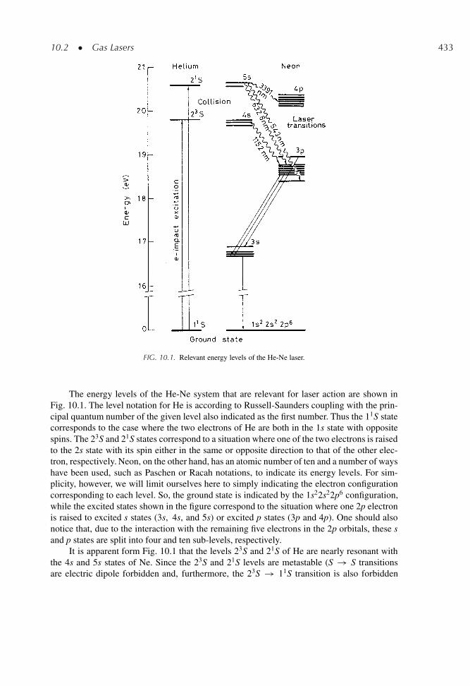
10.2 � Gas Lasers 433
FIG. 10.1. Relevant energy levels of the He-Ne laser.
The energy levels of the He-Ne system that are relevant for laser action are shown inFig. 10.1. The level notation for He is according to Russell-Saunders coupling with the prin-cipal quantum number of the given level also indicated as the first number. Thus the 11S statecorresponds to the case where the two electrons of He are both in the 1s state with oppositespins. The 23S and 21S states correspond to a situation where one of the two electrons is raisedto the 2s state with its spin either in the same or opposite direction to that of the other elec-tron, respectively. Neon, on the other hand, has an atomic number of ten and a number of wayshave been used, such as Paschen or Racah notations, to indicate its energy levels. For sim-plicity, however, we will limit ourselves here to simply indicating the electron configurationcorresponding to each level. So, the ground state is indicated by the 1s22s22p6 configuration,while the excited states shown in the figure correspond to the situation where one 2p electronis raised to excited s states (3s, 4s, and 5s) or excited p states (3p and 4p). One should alsonotice that, due to the interaction with the remaining five electrons in the 2p orbitals, these sand p states are split into four and ten sub-levels, respectively.
It is apparent form Fig. 10.1 that the levels 23S and 21S of He are nearly resonant withthe 4s and 5s states of Ne. Since the 23S and 21S levels are metastable (S ! S transitionsare electric dipole forbidden and, furthermore, the 23S ! 11S transition is also forbidden
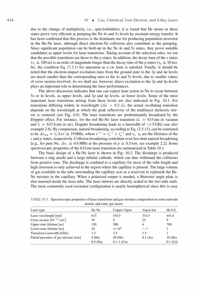
434 10 � Gas, Chemical, Free Electron, and X-Ray Lasers
due to the change of multiplicity, i.e., spin-forbidden), it is found that He atoms in thesestates prove very efficient at pumping the Ne 4s and 5s levels by resonant energy transfer. Ithas been confirmed that this process is the dominant one for producing population inversionin the He-Ne laser, although direct electron-Ne collisions also contribute to the pumping.Since significant population can be built-up in the Ne 4s and 5s states, they prove suitablecandidates as upper levels for laser transitions. Taking account of the selection rules, we seethat the possible transitions are those to the p states. In addition, the decay time of the s states.�s Š 100 ns/ is an order of magnitude longer than the decay time of the p states .�p Š 10 ns/.So, the condition Eq. (7.3.1) for operation as a cw laser is satisfied. Finally, it should benoted that the electron-impact excitation rates from the ground state to the 3p and 4p levelsare much smaller than the corresponding rates to the 4s and 5s levels, due to smaller valuesof cross section involved. As we shall see, however, direct excitation to the 3p and 4p levelsplays an important role in determining the laser performances.
The above discussion indicates that one can expect laser action in Ne to occur between5s or 4s levels, as upper levels, and 3p and 4p levels, as lower levels. Some of the mostimportant laser transitions arising from these levels are also indicated in Fig. 10.1. Fortransitions differing widely in wavelength .� > 0.2 �/, the actual oscillating transitiondepends on the wavelength at which the peak reflectivity of the multilayer dielectric mir-ror is centered (see Fig. 4.9). The laser transitions are predominantly broadened by theDoppler effect. For instance, for the red He-Ne laser transition (� D 633 nm in vacuumand � D 632.8 nm in air), Doppler broadening leads to a linewidth of �1.5 GHz (see alsoexample 2.6). By comparison, natural broadening, according to Eq. (2.5.13), can be estimatedto be �nat D 1=2 � Š 19 MHz, where ��1 D ��1
s C ��1p and �s, �p are the lifetimes of the
s and p states, respectively. Collision broadening contribute even less than natural broadening[e.g., for pure Ne, �c Š 0.6 MHz at the pressure of p Š 0.5 torr, see example 2.2]. Somespectroscopic properties of the 633 nm laser transition are summarized in Table 10.1.
The basic design of a He-Ne laser is shown in Fig. 10.2. The discharge is producedbetween a ring anode and a large tubular cathode, which can thus withstand the collisionsfrom positive ions. The discharge is confined to a capillary for most of the tube length andhigh inversion is only achieved in the region where the capillary is present. The large volumeof gas available in the tube surrounding the capillary acts as a reservoir to replenish the He-Ne mixture in the capillary. When a polarized output is needed, a Brewster angle plate isalso inserted inside the laser tube. The laser mirrors are directly sealed to the two tube ends.The most commonly used resonator configuration is nearly hemispherical since this is easy
TABLE 10.1. Spectroscopic properties of laser transitions and gas-mixture composition in some relevantatomic and ionic gas lasers
Laser type He-Ne Copper Vapor Argon Ion He-Cd
Laser wavelength [nm] 633 510.5 514.5 441.6Cross-section Œ10�14 cm2� 30 9 25 9Upper-state lifetime [ns] 150 500 6 700Lower-state lifetime [ns] 10 � 104 � 1 1Transition Linewidth [GHz] 1.5 2.5 3.5 1Partial pressures of gas mixture [torr] 4 (He) 40 (He) 0.1 (Ar) 10 (He)
0.8 (Ne) 0.1–1 (Cu) 0.1 (Cd)
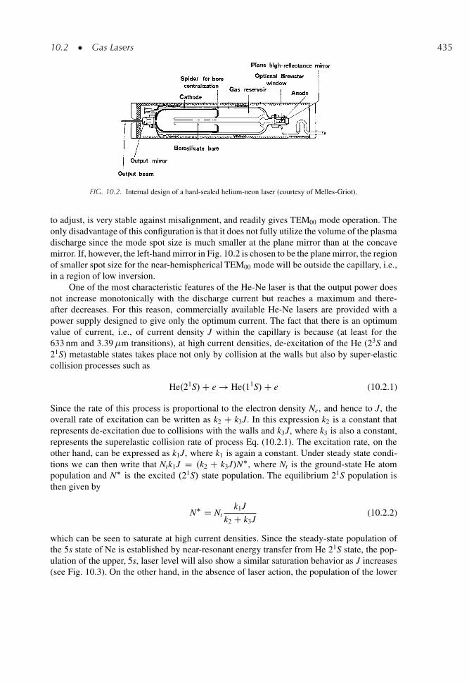
10.2 � Gas Lasers 435
FIG. 10.2. Internal design of a hard-sealed helium-neon laser (courtesy of Melles-Griot).
to adjust, is very stable against misalignment, and readily gives TEM00 mode operation. Theonly disadvantage of this configuration is that it does not fully utilize the volume of the plasmadischarge since the mode spot size is much smaller at the plane mirror than at the concavemirror. If, however, the left-hand mirror in Fig. 10.2 is chosen to be the plane mirror, the regionof smaller spot size for the near-hemispherical TEM00 mode will be outside the capillary, i.e.,in a region of low inversion.
One of the most characteristic features of the He-Ne laser is that the output power doesnot increase monotonically with the discharge current but reaches a maximum and there-after decreases. For this reason, commercially available He-Ne lasers are provided with apower supply designed to give only the optimum current. The fact that there is an optimumvalue of current, i.e., of current density J within the capillary is because (at least for the633 nm and 3.39�m transitions), at high current densities, de-excitation of the He (23S and21S) metastable states takes place not only by collision at the walls but also by super-elasticcollision processes such as
He.21S/C e ! He.11S/C e (10.2.1)
Since the rate of this process is proportional to the electron density Ne, and hence to J, theoverall rate of excitation can be written as k2 C k3J. In this expression k2 is a constant thatrepresents de-excitation due to collisions with the walls and k3J, where k3 is also a constant,represents the superelastic collision rate of process Eq. (10.2.1). The excitation rate, on theother hand, can be expressed as k1J, where k1 is again a constant. Under steady state condi-tions we can then write that Ntk1J D .k2 C k3J/N�, where Nt is the ground-state He atompopulation and N� is the excited .21S/ state population. The equilibrium 21S population isthen given by
N� D Ntk1J
k2 C k3J(10.2.2)
which can be seen to saturate at high current densities. Since the steady-state population ofthe 5s state of Ne is established by near-resonant energy transfer from He 21S state, the pop-ulation of the upper, 5s, laser level will also show a similar saturation behavior as J increases(see Fig. 10.3). On the other hand, in the absence of laser action, the population of the lower
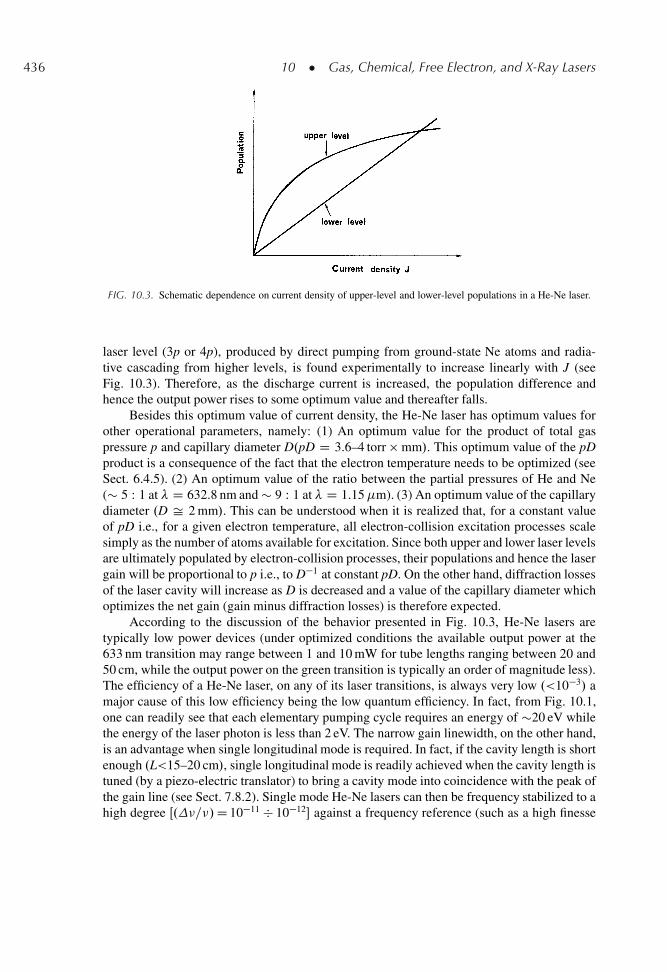
436 10 � Gas, Chemical, Free Electron, and X-Ray Lasers
FIG. 10.3. Schematic dependence on current density of upper-level and lower-level populations in a He-Ne laser.
laser level (3p or 4p), produced by direct pumping from ground-state Ne atoms and radia-tive cascading from higher levels, is found experimentally to increase linearly with J (seeFig. 10.3). Therefore, as the discharge current is increased, the population difference andhence the output power rises to some optimum value and thereafter falls.
Besides this optimum value of current density, the He-Ne laser has optimum values forother operational parameters, namely: (1) An optimum value for the product of total gaspressure p and capillary diameter D.pD D 3.6–4 torr � mm/. This optimum value of the pDproduct is a consequence of the fact that the electron temperature needs to be optimized (seeSect. 6.4.5). (2) An optimum value of the ratio between the partial pressures of He and Ne(� 5 : 1 at � D 632.8 nm and � 9 : 1 at � D 1.15�m). (3) An optimum value of the capillarydiameter .D Š 2 mm/. This can be understood when it is realized that, for a constant valueof pD i.e., for a given electron temperature, all electron-collision excitation processes scalesimply as the number of atoms available for excitation. Since both upper and lower laser levelsare ultimately populated by electron-collision processes, their populations and hence the lasergain will be proportional to p i.e., to D�1 at constant pD. On the other hand, diffraction lossesof the laser cavity will increase as D is decreased and a value of the capillary diameter whichoptimizes the net gain (gain minus diffraction losses) is therefore expected.
According to the discussion of the behavior presented in Fig. 10.3, He-Ne lasers aretypically low power devices (under optimized conditions the available output power at the633 nm transition may range between 1 and 10 mW for tube lengths ranging between 20 and50 cm, while the output power on the green transition is typically an order of magnitude less).The efficiency of a He-Ne laser, on any of its laser transitions, is always very low .<10�3/ amajor cause of this low efficiency being the low quantum efficiency. In fact, from Fig. 10.1,one can readily see that each elementary pumping cycle requires an energy of �20 eV whilethe energy of the laser photon is less than 2 eV. The narrow gain linewidth, on the other hand,is an advantage when single longitudinal mode is required. In fact, if the cavity length is shortenough .L<15–20 cm/, single longitudinal mode is readily achieved when the cavity length istuned (by a piezo-electric translator) to bring a cavity mode into coincidence with the peak ofthe gain line (see Sect. 7.8.2). Single mode He-Ne lasers can then be frequency stabilized to ahigh degree Œ.�=�/D 10�11 � 10�12� against a frequency reference (such as a high finesse
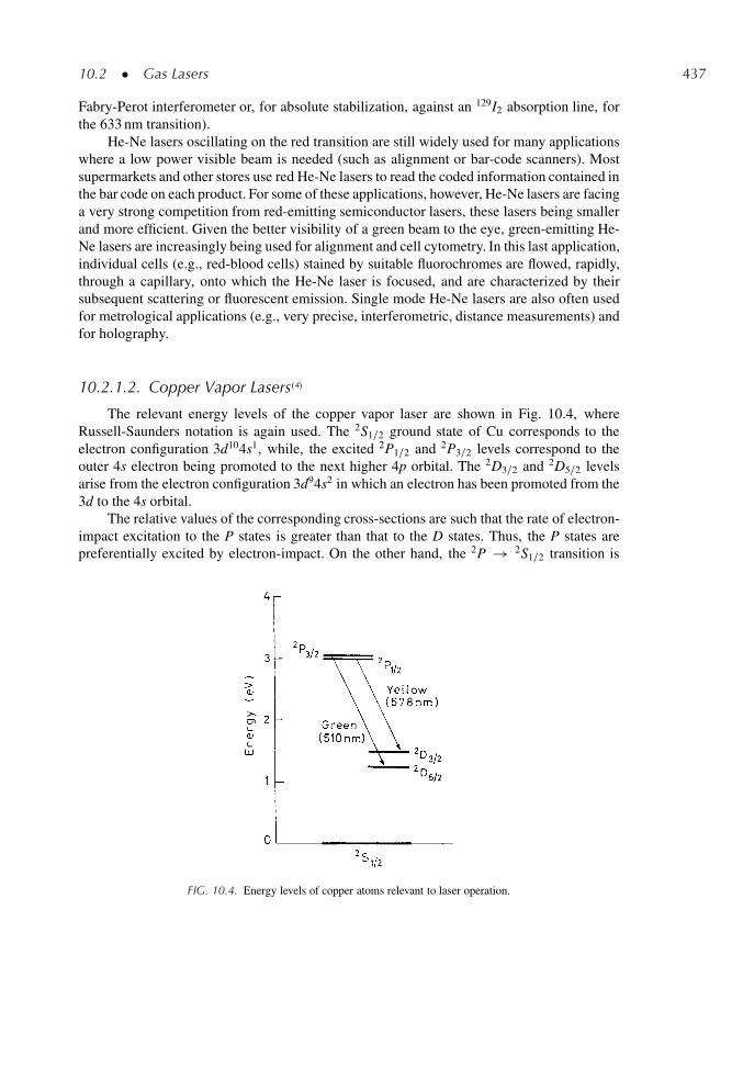
10.2 � Gas Lasers 437
Fabry-Perot interferometer or, for absolute stabilization, against an 129I2 absorption line, forthe 633 nm transition).
He-Ne lasers oscillating on the red transition are still widely used for many applicationswhere a low power visible beam is needed (such as alignment or bar-code scanners). Mostsupermarkets and other stores use red He-Ne lasers to read the coded information contained inthe bar code on each product. For some of these applications, however, He-Ne lasers are facinga very strong competition from red-emitting semiconductor lasers, these lasers being smallerand more efficient. Given the better visibility of a green beam to the eye, green-emitting He-Ne lasers are increasingly being used for alignment and cell cytometry. In this last application,individual cells (e.g., red-blood cells) stained by suitable fluorochromes are flowed, rapidly,through a capillary, onto which the He-Ne laser is focused, and are characterized by theirsubsequent scattering or fluorescent emission. Single mode He-Ne lasers are also often usedfor metrological applications (e.g., very precise, interferometric, distance measurements) andfor holography.
10.2.1.2. Copper Vapor Lasers.4/
The relevant energy levels of the copper vapor laser are shown in Fig. 10.4, whereRussell-Saunders notation is again used. The 2S1=2 ground state of Cu corresponds to theelectron configuration 3d104s1, while, the excited 2P1=2 and 2P3=2 levels correspond to theouter 4s electron being promoted to the next higher 4p orbital. The 2D3=2 and 2D5=2 levelsarise from the electron configuration 3d94s2 in which an electron has been promoted from the3d to the 4s orbital.
The relative values of the corresponding cross-sections are such that the rate of electron-impact excitation to the P states is greater than that to the D states. Thus, the P states arepreferentially excited by electron-impact. On the other hand, the 2P ! 2S1=2 transition is
FIG. 10.4. Energy levels of copper atoms relevant to laser operation.
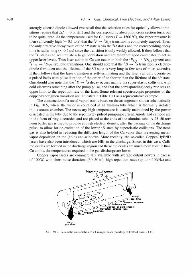
438 10 � Gas, Chemical, Free Electron, and X-Ray Lasers
strongly electric-dipole allowed (we recall that the selection rules for optically allowed tran-sitions require that J D 0 or ˙1) and the corresponding absorption cross section turns outto be quite large. At the temperature used for Cu lasers .T D 1500 ıC/, the vapor pressure isthen sufficiently high (� 0.1 torr) that the 2P ! 2S1=2 transition is completely trapped. Thus,the only effective decay route of the 2P state is via the 2D states and the corresponding decaytime is rather long .� 0.5 μs/ since the transition is only weakly allowed. It then follows thatthe 2P states can accumulate a large population and are therefore good candidates to act asupper laser levels. Thus laser action in Cu can occur on both the 2P3=2 ! 2D5=2 (green) and2P1=2 ! 2D3=2 (yellow) transitions. One should note that the 2D ! 2S transition is electric-dipole forbidden and the lifetime of the 2D state is very long (a few tens of microseconds).It then follows that the laser transition is self-terminating and the laser can only operate ona pulsed basis with pulse duration of the order of or shorter than the lifetime of the 2P state.One should also note that the 2D ! 2S decay occurs mainly via super-elastic collisions withcold electrons remaining after the pump pulse, and that the corresponding decay rate sets anupper limit to the repetition rate of the laser. Some relevant spectroscopic properties of thecopper-vapor green transition are indicated in Table 10.1 as a representative example.
The construction of a metal vapor laser is based on the arrangement shown schematicallyin Fig. 10.5, where the vapor is contained in an alumina tube which is thermally isolatedin a vacuum chamber. The necessary high temperature is usually maintained by the powerdissipated in the tube due to the repetitively pulsed pumping-current. Anode and cathode arein the form of ring electrodes and are placed at the ends of the alumina tube. A 25–50 torrneon buffer gas is used to provide enough electron density, after the passage of the dischargepulse, to allow for de-excitation of the lower 2D state by superelastic collisions. The neongas is also helpful in reducing the diffusion length of the Cu vapor thus preventing metal-vapor deposition on the (cold) end-windows. More recently, the so-called Copper-HyBrIDlasers have also been introduced, which use HBr in the discharge. Since, in this case, CuBrmolecules are formed in the discharge region and these molecules are much more volatile thanCu atoms, the temperatures required in the gas discharge are lower.
Copper vapor lasers are commercially available with average output powers in excessof 100 W, with short pulse durations (30–50 ns), high repetition rates (up to �10 kHz) and
FIG. 10.5. Schematic construction of a Cu-vapor laser (courtesy of Oxford Lasers, Ltd).
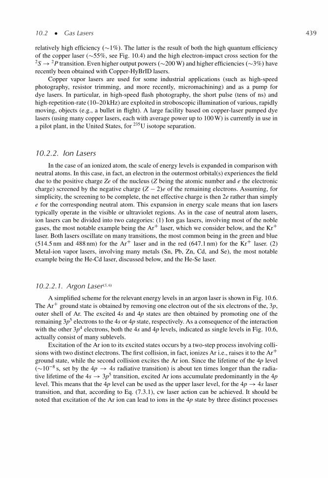
10.2 � Gas Lasers 439
relatively high efficiency .�1%/. The latter is the result of both the high quantum efficiencyof the copper laser (�55%, see Fig. 10.4) and the high electron-impact cross section for the2S ! 2P transition. Even higher output powers .�200 W/ and higher efficiencies .�3%/ haverecently been obtained with Copper-HyBrID lasers.
Copper vapor lasers are used for some industrial applications (such as high-speedphotography, resistor trimming, and more recently, micromachining) and as a pump fordye lasers. In particular, in high-speed flash photography, the short pulse (tens of ns) andhigh-repetition-rate (10–20 kHz) are exploited in stroboscopic illumination of various, rapidlymoving, objects (e.g., a bullet in flight). A large facility based on copper-laser pumped dyelasers (using many copper lasers, each with average power up to 100 W) is currently in use ina pilot plant, in the United States, for 235U isotope separation.
10.2.2. Ion Lasers
In the case of an ionized atom, the scale of energy levels is expanded in comparison withneutral atoms. In this case, in fact, an electron in the outermost orbital(s) experiences the fielddue to the positive charge Ze of the nucleus (Z being the atomic number and e the electroniccharge) screened by the negative charge .Z � 2/e of the remaining electrons. Assuming, forsimplicity, the screening to be complete, the net effective charge is then 2e rather than simplye for the corresponding neutral atom. This expansion in energy scale means that ion laserstypically operate in the visible or ultraviolet regions. As in the case of neutral atom lasers,ion lasers can be divided into two categories: (1) Ion gas lasers, involving most of the noblegases, the most notable example being the ArC laser, which we consider below, and the KrClaser. Both lasers oscillate on many transitions, the most common being in the green and blue(514.5 nm and 488 nm) for the ArC laser and in the red (647.1 nm) for the KrC laser. (2)Metal-ion vapor lasers, involving many metals (Sn, Pb, Zn, Cd, and Se), the most notableexample being the He-Cd laser, discussed below, and the He-Se laser.
10.2.2.1. Argon Laser.5,6/
A simplified scheme for the relevant energy levels in an argon laser is shown in Fig. 10.6.The ArC ground state is obtained by removing one electron out of the six electrons of the, 3p,outer shell of Ar. The excited 4s and 4p states are then obtained by promoting one of theremaining 3p5 electrons to the 4s or 4p state, respectively. As a consequence of the interactionwith the other 3p4 electrons, both the 4s and 4p levels, indicated as single levels in Fig. 10.6,actually consist of many sublevels.
Excitation of the Ar ion to its excited states occurs by a two-step process involving colli-sions with two distinct electrons. The first collision, in fact, ionizes Ar i.e., raises it to the ArCground state, while the second collision excites the Ar ion. Since the lifetime of the 4p level(�10�8 s, set by the 4p ! 4s radiative transition) is about ten times longer than the radia-tive lifetime of the 4s ! 3p5 transition, excited Ar ions accumulate predominantly in the 4plevel. This means that the 4p level can be used as the upper laser level, for the 4p ! 4s lasertransition, and that, according to Eq. (7.3.1), cw laser action can be achieved. It should benoted that excitation of the Ar ion can lead to ions in the 4p state by three distinct processes
440 10 � Gas, Chemical, Free Electron, and X-Ray Lasers
FIG. 10.6. Energy levels of Ar relevant for laser action.
(see Fig. 10.6): (a) direct excitation to the 4p level starting from the ArC ground level; (b)excitation to higher-lying states followed by radiative decay to the 4p level; (c) excitation tometastable levels followed by a third collision leading to excitation to the 4p state. Consider-ing, for simplicity, only processes (a) and (b) one can readily see that the pumping process tothe upper state is expected to be proportional to the square of the discharge current density. Infact, since processes (a) and (b) involve a two-steps electron collision, the rate of upper stateexcitation, .dN2=dt/p, is expected to be of the form
.dN2=dt/p / NeNi Š N2e (10.2.3)
where Ne and Ni are the electron and ion density in the plasma (Ne Š Ni in the positivecolumn of the plasma). Since the electric field of the discharge is independent of the dischargecurrent, the drift velocity, �drift, will also be independent of the discharge current. From thestandard equation J D e�driftNe, one then see that the electron density Ne is proportional tothe discharge current density, and, from Eq. (10.2.3) it follows that .dN2=dt/p / J2. Laserpumping thus increases rapidly with current density and high current densities .�1 kA=cm2/
are required if the inherently inefficient two-step processes, considered above, are to pumpenough ions to the upper state. This may explain why the first operation of an ArC laseroccurred some three-years after the first He-Ne laser..7/
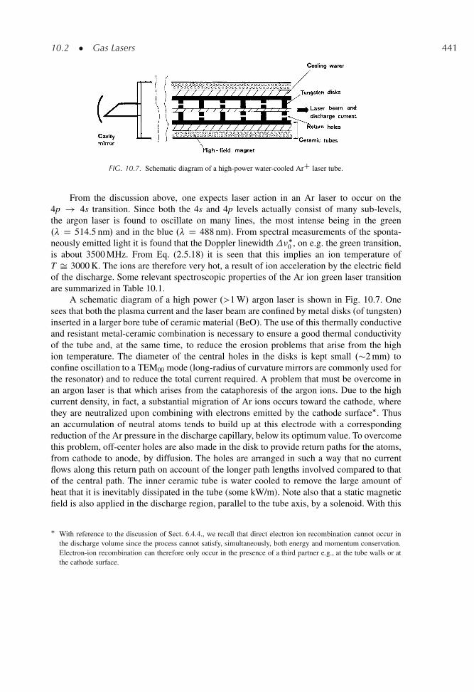
10.2 � Gas Lasers 441
FIG. 10.7. Schematic diagram of a high-power water-cooled ArC laser tube.
From the discussion above, one expects laser action in an Ar laser to occur on the4p ! 4s transition. Since both the 4s and 4p levels actually consist of many sub-levels,the argon laser is found to oscillate on many lines, the most intense being in the green.� D 514.5 nm/ and in the blue .� D 488 nm/. From spectral measurements of the sponta-neously emitted light it is found that the Doppler linewidth ��
0 , on e.g. the green transition,is about 3500 MHz. From Eq. (2.5.18) it is seen that this implies an ion temperature ofT Š 3000 K. The ions are therefore very hot, a result of ion acceleration by the electric fieldof the discharge. Some relevant spectroscopic properties of the Ar ion green laser transitionare summarized in Table 10.1.
A schematic diagram of a high power .>1 W/ argon laser is shown in Fig. 10.7. Onesees that both the plasma current and the laser beam are confined by metal disks (of tungsten)inserted in a larger bore tube of ceramic material (BeO). The use of this thermally conductiveand resistant metal-ceramic combination is necessary to ensure a good thermal conductivityof the tube and, at the same time, to reduce the erosion problems that arise from the highion temperature. The diameter of the central holes in the disks is kept small .�2 mm/ toconfine oscillation to a TEM00 mode (long-radius of curvature mirrors are commonly used forthe resonator) and to reduce the total current required. A problem that must be overcome inan argon laser is that which arises from the cataphoresis of the argon ions. Due to the highcurrent density, in fact, a substantial migration of Ar ions occurs toward the cathode, wherethey are neutralized upon combining with electrons emitted by the cathode surface�. Thusan accumulation of neutral atoms tends to build up at this electrode with a correspondingreduction of the Ar pressure in the discharge capillary, below its optimum value. To overcomethis problem, off-center holes are also made in the disk to provide return paths for the atoms,from cathode to anode, by diffusion. The holes are arranged in such a way that no currentflows along this return path on account of the longer path lengths involved compared to thatof the central path. The inner ceramic tube is water cooled to remove the large amount ofheat that it is inevitably dissipated in the tube (some kW/m). Note also that a static magneticfield is also applied in the discharge region, parallel to the tube axis, by a solenoid. With this
� With reference to the discussion of Sect. 6.4.4., we recall that direct electron ion recombination cannot occur inthe discharge volume since the process cannot satisfy, simultaneously, both energy and momentum conservation.Electron-ion recombination can therefore only occur in the presence of a third partner e.g., at the tube walls or atthe cathode surface.
442 10 � Gas, Chemical, Free Electron, and X-Ray Lasers
arrangement, the Lorentz force makes the electrons rotate around the tube axis, thus reducingthe rate of electron diffusion to the walls. This increases the number of free electrons at thecenter of the tube and leads to an increased pump rate. This may explain the observed increasein output power when a magnetic field is applied. By confining the charges toward the centerof the tube, the magnetic field also alleviates the problem of wall damage (mostly occurringat the holes of the tungsten disks). Note that, for high power lasers .>1 W/, the laser mirrorsare mounted externally to the laser tube to reduce degradation of the mirror coatings due tothe intense VUV radiation emitted by the plasma. For lower-power lasers .<1 W/, the lasertube is often simply made of a block of ceramic (BeO) provided with a central hole for thedischarge current. In this case, no magnetic field is applied, the tube is air cooled, and themirrors are directly sealed to the ends of the tube as in a He-Ne laser.
Water-cooled argon lasers are commercially available with power ranging between 1and 20 W, operating on both blue and green transitions simultaneously or, by using the con-figuration of Fig. 7.16b, operating on a single line. Air-cooled argon lasers of lower power.�100 mW/ and much simpler design are also commercially available. In both cases, onceabove threshold, the output power increases rapidly with current density ./ J2/ since, bycontrast with the behavior of He-Ne lasers, in this case there is no process leading to sat-uration of inversion. The laser efficiency is, however, very low .<10�3/, because the laserquantum efficiency is rather low (�7.5%, see Fig. 10.6) and because the electron impact exci-tation involves many levels that are not coupled effectively to the upper laser level. Argonlasers are often operated in mode-locked regime using an acousto-optic modulator. In thiscase, fairly short mode-locked laser pulses .�150 ps/ are achievable by virtue of the relativelylarge transition line-width .�3.5 GHz/ which, furthermore, is inhomogeneously broadened.
Argon lasers are widely used in ophthalmology (particularly to cure diabetic retinopa-thy), and in the field of laser entertainment (laser light shows). In a more scientifically-orientedcontest, argon lasers are also widely used for a variety of studies of light-matter interaction(particularly in mode-locked operation) and also as a pump for solid-state lasers (particularlyTi:sapphire) and dye lasers. For many of these applications, argon lasers are tending to besuperseded now by cw diode-pumped Nd : YVO4 lasers in which a green beam, λ D 532 nm,is produced by intracavity second harmonic generation. Lower-power Ar lasers are extensivelyused for high-speed laser printers and cell cytometry.
10.2.2.2. He-Cd Laser
The energy levels of the He-Cd system that are relevant for laser action are shown inFig. 10.8, where, again, level labeling is according to Russell-Saunders notation. Pumping ofCdC upper laser levels .2D3=2 and 2D5=2/ is achieved with the help of He through the Penningionization process. This process can be written in the general form
A� C B ! A C BC C e (10.2.4)
where the ion BC may or may not be left in an excited state. Of course, the process can onlyoccur if the excitation energy of the excited species A� is greater than or equal to the ionizationenergy of species B (plus the excitation energy of BC if the ion is left in an excited state). Notethat, unlike near-resonant energy transfer, Penning ionization is a non-resonant process, anysurplus energy being in fact released as kinetic energy of the ejected electron. In the case of the
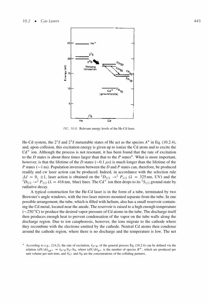
10.2 � Gas Lasers 443
FIG. 10.8. Relevant energy levels of the He-Cd laser.
He-Cd system, the 21S and 23S metastable states of He act as the species A� in Eq. (10.2.4),and, upon collision, this excitation energy is given up to ionize the Cd atom and to excite theCdC ion. Although the process is not resonant, it has been found that the rate of excitationto the D states is about three times larger than that to the P states�. What is more important,however, is that the lifetime of the D states .�0.1�s/ is much longer than the lifetime of theP states .�1 ns/. Population inversion between the D and P states can, therefore, be producedreadily and cw laser action can be produced. Indeed, in accordance with the selection ruleJ D 0, ˙1, laser action is obtained on the 2D3=2 !2 P1=2 .� D 325 nm, UV/ and the2D5=2 !2 P3=2 .� D 416 nm, blue/ lines. The CdC ion then drops to its 2S1=2 ground state byradiative decay.
A typical construction for the He-Cd laser is in the form of a tube, terminated by twoBrewster’s angle windows, with the two laser mirrors mounted separate from the tube. In onepossible arrangement, the tube, which is filled with helium, also has a small reservoir contain-ing the Cd metal, located near the anode. The reservoir is raised to a high enough temperature.�250 ıC/ to produce the desired vapor pressure of Cd atoms in the tube. The discharge itselfthen produces enough heat to prevent condensation of the vapor on the tube walls along thedischarge region. Due to ion cataphoresis, however, the ions migrate to the cathode wherethey recombine with the electrons emitted by the cathode. Neutral Cd atoms then condensearound the cathode region, where there is no discharge and the temperature is low. The net
� According to e.g., (2.6.2), the rate of excitation, kA�B, of the general process Eq. (10.2.4) can be defined via therelation .dN=dt/ABC D kA�B NA� NB, where .dN=dt/BC is the number of species BC, which are produced perunit volume per unit time, and NA� and NB are the concentrations of the colliding partners.
444 10 � Gas, Chemical, Free Electron, and X-Ray Lasers
result is a continuous flow of metal vapor from the anode to the cathode. Therefore a sufficientsupply of Cd (�1 g per 1,000 h) must be provided for long-term operation of the laser.
He-Cd lasers can give output powers of 50–100 mW, placing them in an intermediateposition between red He-Ne lasers (a few mW) and ArC lasers (a few W). Thus, He-Cd lasersare used for many applications where a blue or UV beam of moderate power is required (e.g.,high-speed laser printers, holography, cell cytometry, fluorescence analysis of e.g., biologicalspecimens).
10.2.3. Molecular Gas Lasers
These lasers exploit transitions between the energy levels of a molecule. Depending onthe type of transition involved, molecular gas lasers belong to one of the three following cate-gories: (1) Vibrational-rotational lasers. These lasers use transitions between vibrational levelsof the same electronic state (the ground state) and the energy difference between the levelsfalls in the middle- to the far-infrared .2.5–300�m/. By far the most important example ofthis category is the CO2 laser oscillating at either 10.6 or 9.6�m. Other noteworthy examplesare the CO laser .� Š 5�m/ and the HF chemical laser .� Š 2.7–3.3�m/. (2) Vibroniclasers, which use transitions between vibrational levels of different electronics states: In thiscase the oscillation wavelength generally falls in the UV region. The most notable example ofthis category of laser is the nitrogen laser .� D 337 nm/. A special class of lasers, which canperhaps be included in the vibronic lasers, is the excimer laser. These lasers involve transitionsbetween different electronic states of special molecules (excimers) with corresponding emis-sion wavelengths generally in the UV. Excimer lasers, however, involve not only transitionsbetween bound states (bound-bound transitions) but also, and actually more often, transitionsbetween a bound upper state and a repulsive ground state (bound-free transitions). It is moreappropriate therefore to treat these lasers as being in a category of their own. (3) Pure rota-tional lasers, which use transitions between different rotational levels of the same vibrationalstate (usually an excited vibrational level of the ground electronic state). The correspondingwavelength falls in the far infrared (25�m to 1 mm). Since these pure rotational lasers arerelatively less important than the other categories, we shall not discuss them further in thesections that follow. We therefore limit ourselves to pointing out here that laser action is moredifficult to achieve in this type of laser since the relaxation between rotational levels is gener-ally very fast. Therefore these lasers are usually pumped optically, using the output of anotherlaser as the pump (commonly a CO2 laser). Optical pumping excites the given molecule (e.g.,CH3F, � D 496�m) to a rotational level belonging to some vibrational state above the groundlevel. Laser action then takes place between rotational levels of this upper vibrational state.
10.2.3.1. The CO2 Laser.8,9/
The laser utilizes, as active medium, a suitable mixture of CO2, N2, and He. Oscillationtakes place between two vibrational levels of the CO2 molecule, while, as we shall see, theN2 and He greatly improve the efficiency of laser action. The CO2 laser is actually one of themost powerful lasers (output powers of more than 100 kW have been demonstrated from aCO2 gas-dynamic laser) and one of the most efficient (15–20% slope efficiency).
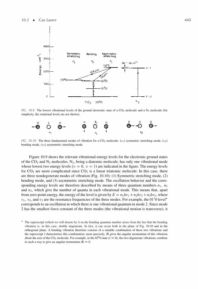
10.2 � Gas Lasers 445
FIG. 10.9. The lowest vibrational levels of the ground electronic state of a CO2 molecule and a N2 molecule (forsimplicity, the rotational levels are not shown).
FIG. 10.10. The three fundamental modes of vibration for a CO2 molecule: .�1/ symmetric stretching mode, .�2/
bending mode, .�3/ asymmetric stretching mode.
Figure 10.9 shows the relevant vibrational-energy levels for the electronic ground statesof the CO2 and N2 molecules. N2, being a diatomic molecule, has only one vibrational modewhose lowest two energy levels .� D 0, � D 1/ are indicated in the figure. The energy levelsfor CO2 are more complicated since CO2 is a linear triatomic molecule. In this case, thereare three nondegenerate modes of vibration (Fig. 10.10): (1) Symmetric stretching mode, (2)bending mode, and (3) asymmetric stretching mode. The oscillation behavior and the corre-sponding energy levels are therefore described by means of three quantum numbers n1, n2
and n3, which give the number of quanta in each vibrational mode. This means that, apartfrom zero-point energy, the energy of the level is given by E D n1h�1 Cn2h�2 Cn3h�3, where�1, �2, and �3 are the resonance frequencies of the three modes. For example, the 0110 level�corresponds to an oscillation in which there is one vibrational quantum in mode 2. Since mode2 has the smallest force constant of the three modes (the vibrational motion is transverse), it
� The superscript (which we will denote by l) on the bending quantum number arises from the fact that the bendingvibration is, in this case, doubly degenerate. In fact, it can occur both in the plane of Fig. 10.10 and in theorthogonal plane. A bending vibration therefore consists of a suitable combination of these two vibrations andthe superscript l characterizes this combination; more precisely, l„ gives the angular momentum of this vibrationabout the axis of the CO2 molecule. For example, in the 0200 state .l D 0/, the two degenerate vibrations combinein such a way to give an angular momentum l„ D 0.
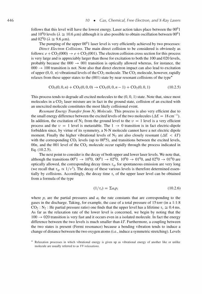
446 10 � Gas, Chemical, Free Electron, and X-Ray Lasers
follows that this level will have the lowest energy. Laser action takes place between the 0001and 1000 levels .� Š 10.6�m/ although it is also possible to obtain oscillation between 0001and 0200 .� Š 9.6�m/.
The pumping of the upper 0001 laser level is very efficiently achieved by two processes:Direct Electron Collisions. The main direct collision to be considered is obviously as
follows: e C CO2.000/ ! e C CO2.001/. The electron collision cross section for this processis very large and is appreciably larger than those for excitation to both the 100 and 020 levels,probably because the 000 ! 001 transition is optically allowed whereas, for instance, the000 ! 100 transition is not. Note also that direct electron impact can also lead to excitationof upper .0, 0, n/ vibrational levels of the CO2 molecule. The CO2 molecule, however, rapidlyrelaxes from these upper states to the (001) state by near resonant collisions of the type�
CO2.0, 0, n/C CO2.0, 0, 0/ ! CO2.0, 0, n � 1/C CO2.0, 0, 1/ (10.2.5)
This process tends to degrade all excited molecules to the (0, 0, 1) state. Note that, since mostmolecules in a CO2 laser mixture are in fact in the ground state, collision of an excited withan unexcited molecule constitutes the most likely collisional event.
Resonant Energy Transfer from N2 Molecule. This process is also very efficient due tothe small energy difference between the excited levels of the two molecules .E D 18 cm�1/.In addition, the excitation of N2 from the ground level to the � D 1 level is a very efficientprocess and the � D 1 level is metastable. The 1 ! 0 transition is in fact electric-dipoleforbidden since, by virtue of its symmetry, a N-N molecule cannot have a net electric dipolemoment. Finally the higher vibrational levels of N2 are also closely resonant .E < kT/with the corresponding CO2 levels (up to 0005), and transitions between the excited levels,00n, and the 001 level of the CO2 molecule occur rapidly through the process indicated inEq. (10.2.5).
The next point to consider is the decay of both upper and lower laser levels. We note that,although the transitions 0001 ! 1000, 0001 ! 0200, 1000 ! 0100, and 0200 ! 0100 areoptically allowed, the corresponding decay times �sp for spontaneous emission are very long(we recall that �sp / 1=�3). The decay of these various levels is therefore determined essen-tially by collisions. Accordingly, the decay time �s of the upper laser level can be obtainedfrom a formula of the type
.1=�s/ D †aipi (10.2.6)
where pi are the partial pressures and ai the rate constants that are corresponding to thegases in the discharge. Taking, for example, the case of a total pressure of 15 torr (in a 1:1:8CO2 : N2 : He partial pressure ratio) one finds that the upper level has a lifetime �s Š 0.4 ms.As far as the relaxation rate of the lower level is concerned, we begin by noting that the100 ! 020 transition is very fast and it occurs even in a isolated molecule. In fact the energydifference between the two levels is much smaller than kT. Furthermore, a coupling betweenthe two states is present (Fermi resonance) because a bending vibration tends to induce achange of distance between the two oxygen atoms (i.e., induce a symmetric stretching). Levels
� Relaxation processes in which vibrational energy is given up as vibrational energy of another like or unlikemolecule are usually referred to as VV relaxations.
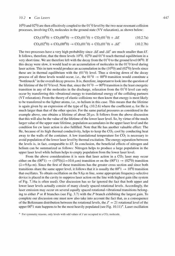
10.2 � Gas Lasers 447
1000 and 0200 are then effectively coupled to the 0110 level by the two near-resonant collisionprocesses, involving CO2 molecules in the ground state (VV relaxation), as shown below:
CO2.1000/C CO2.0000/ ! CO2.0110/C CO2.0110/CE (10.2.7a)
CO2.0200/C CO2.0000/ ! CO2.0110/C CO2.0110/CE0 (10.2.7b)
The two processes have a very high probability since E and E0 are much smaller than kT.It follows, therefore, that the three levels 1000, 0200 and 0110 reach thermal equilibrium in avery short time. We are therefore left with the decay from the 0110 to the ground level 0000. Ifthis decay were slow, it would lead to an accumulation of molecules in the 0110 level duringlaser action. This in turn would produce an accumulation in the .1000/ and .0200/ levels sincethese are in thermal equilibrium with the .0110/ level. Thus a slowing down of the decayprocess of all three levels would occur, i.e., the 0110 ! 0000 transition would constitute a“bottleneck” in the overall decay process. It is, therefore, important to look into the question ofthe lifetime of the 0110 level. Note that, since the 0110 ! 0000 transition is the least energetictransition in any of the molecules in the discharge, relaxation from the 0110 level can onlyoccur by transferring this vibrational energy to translational energy of the colliding partners(VT relaxation). From the theory of elastic collisions we then know that energy is most likelyto be transferred to the lighter atoms, i.e., to helium in this case. This means that the lifetimeis again given by an expression of the type of Eq. (10.2.6) where the coefficient ai for He ismuch larger than that of the other species. For the same partial pressures as considered in theexample above, one obtains a lifetime of about 20�s. It follows from the above discussionthat this will also be the value of the lifetime of the lower laser level. So, by virtue of the muchlarger value of the upper state lifetime, population accumulates in the upper laser level and thecondition for cw laser action is also fulfilled. Note that He has another valuable effect: TheHe, because of its high thermal conductivity, helps to keep the CO2 cool by conducting heataway to the walls of the container. A low translational temperature for CO2 is necessary toavoid population of the lower laser level by thermal excitation. The energy separation betweenthe levels is, in fact, comparable to kT. In conclusion, the beneficial effects of nitrogen andhelium can be summarized as follows: Nitrogen helps to produce a large population in theupper laser level while helium helps to empty population from the lower laser level.
From the above considerations it is seen that laser action in a CO2 laser may occureither on the .0001/ ! .1000/.�D10.6�m/ transition or on the .0001/ ! .0200/ transition.�D9.6�m/. Since the first of these transitions has the greater cross section and since bothtransitions share the same upper level, it follows that it is usually the 0001 ! 1000 transitionthat oscillates. To obtain oscillation on the 9.6�m line, some appropriate frequency-selectivedevice is placed in the cavity to suppress laser action on the line with highest gain (the systemof Fig. 7.16a is often used). Our discussion has so far ignored the fact that both upper andlower laser levels actually consist of many closely spaced rotational levels. Accordingly, thelaser emission may occur on several equally spaced rotational-vibrational transitions belong-ing to either P or R branches (see Fig. 3.7) with the P branch exhibiting the largest gain. Tocomplete our discussion one must now also take into account the fact that, as a consequenceof the Boltzmann distribution between the rotational levels, the J0 D 21 rotational level of theupper 0001 state happens to be the most heavily populated (see Fig. 10.11)�. Laser oscillation
� For symmetry reasons, only levels with odd values of J are occupied in a CO2 molecule.
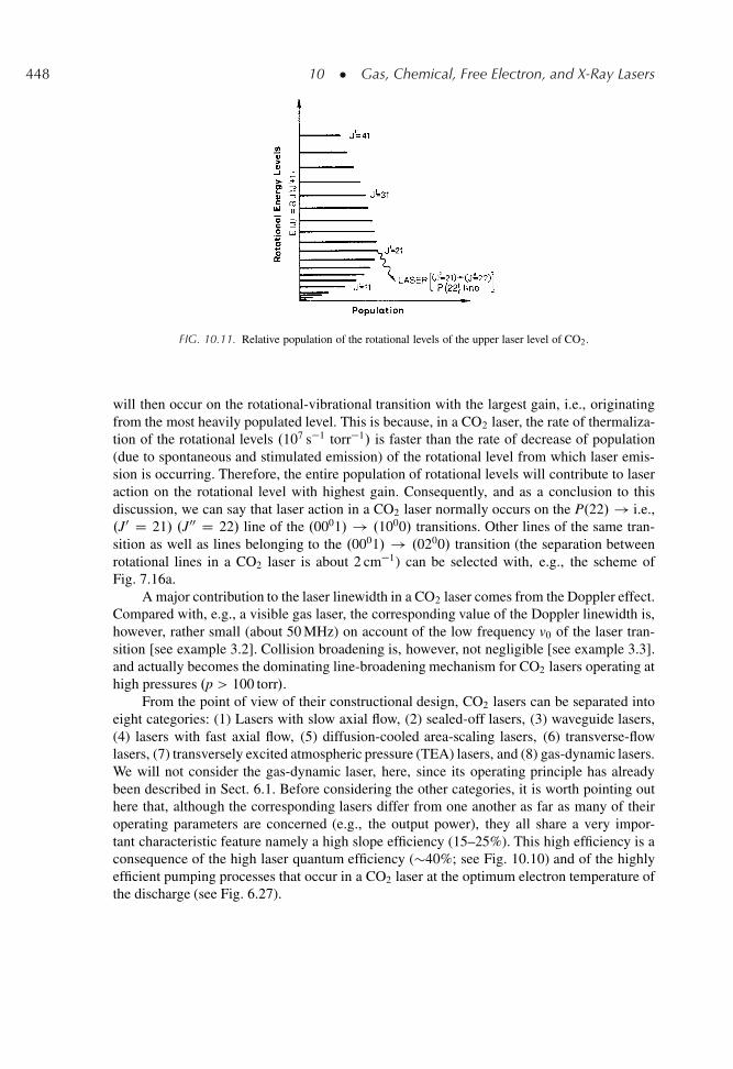
448 10 � Gas, Chemical, Free Electron, and X-Ray Lasers
FIG. 10.11. Relative population of the rotational levels of the upper laser level of CO2.
will then occur on the rotational-vibrational transition with the largest gain, i.e., originatingfrom the most heavily populated level. This is because, in a CO2 laser, the rate of thermaliza-tion of the rotational levels .107 s�1 torr�1/ is faster than the rate of decrease of population(due to spontaneous and stimulated emission) of the rotational level from which laser emis-sion is occurring. Therefore, the entire population of rotational levels will contribute to laseraction on the rotational level with highest gain. Consequently, and as a conclusion to thisdiscussion, we can say that laser action in a CO2 laser normally occurs on the P.22/ ! i.e.,.J0 D 21/ .J00 D 22/ line of the .0001/ ! .1000/ transitions. Other lines of the same tran-sition as well as lines belonging to the .0001/ ! .0200/ transition (the separation betweenrotational lines in a CO2 laser is about 2 cm�1) can be selected with, e.g., the scheme ofFig. 7.16a.
A major contribution to the laser linewidth in a CO2 laser comes from the Doppler effect.Compared with, e.g., a visible gas laser, the corresponding value of the Doppler linewidth is,however, rather small (about 50 MHz) on account of the low frequency v0 of the laser tran-sition [see example 3.2]. Collision broadening is, however, not negligible [see example 3.3].and actually becomes the dominating line-broadening mechanism for CO2 lasers operating athigh pressures .p > 100 torr/.
From the point of view of their constructional design, CO2 lasers can be separated intoeight categories: (1) Lasers with slow axial flow, (2) sealed-off lasers, (3) waveguide lasers,(4) lasers with fast axial flow, (5) diffusion-cooled area-scaling lasers, (6) transverse-flowlasers, (7) transversely excited atmospheric pressure (TEA) lasers, and (8) gas-dynamic lasers.We will not consider the gas-dynamic laser, here, since its operating principle has alreadybeen described in Sect. 6.1. Before considering the other categories, it is worth pointing outhere that, although the corresponding lasers differ from one another as far as many of theiroperating parameters are concerned (e.g., the output power), they all share a very impor-tant characteristic feature namely a high slope efficiency (15–25%). This high efficiency is aconsequence of the high laser quantum efficiency (�40%; see Fig. 10.10) and of the highlyefficient pumping processes that occur in a CO2 laser at the optimum electron temperature ofthe discharge (see Fig. 6.27).
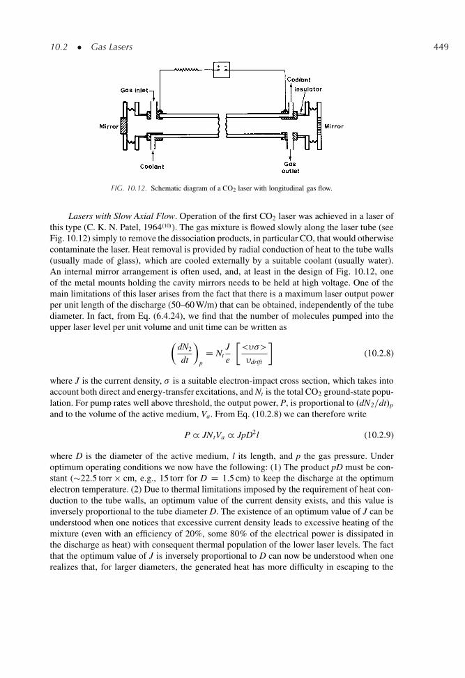
10.2 � Gas Lasers 449
FIG. 10.12. Schematic diagram of a CO2 laser with longitudinal gas flow.
Lasers with Slow Axial Flow. Operation of the first CO2 laser was achieved in a laser ofthis type (C. K. N. Patel, 1964.10/). The gas mixture is flowed slowly along the laser tube (seeFig. 10.12) simply to remove the dissociation products, in particular CO, that would otherwisecontaminate the laser. Heat removal is provided by radial conduction of heat to the tube walls(usually made of glass), which are cooled externally by a suitable coolant (usually water).An internal mirror arrangement is often used, and, at least in the design of Fig. 10.12, oneof the metal mounts holding the cavity mirrors needs to be held at high voltage. One of themain limitations of this laser arises from the fact that there is a maximum laser output powerper unit length of the discharge (50–60 W/m) that can be obtained, independently of the tubediameter. In fact, from Eq. (6.4.24), we find that the number of molecules pumped into theupper laser level per unit volume and unit time can be written as
�dN2
dt
�p
D NtJ
e
�<��>
�drift
�(10.2.8)
where J is the current density, � is a suitable electron-impact cross section, which takes intoaccount both direct and energy-transfer excitations, and Nt is the total CO2 ground-state popu-lation. For pump rates well above threshold, the output power, P, is proportional to .dN2=dt/pand to the volume of the active medium, Va. From Eq. (10.2.8) we can therefore write
P _ JNtVa _ JpD2l (10.2.9)
where D is the diameter of the active medium, l its length, and p the gas pressure. Underoptimum operating conditions we now have the following: (1) The product pD must be con-stant (�22.5 torr � cm, e.g., 15 torr for D D 1.5 cm) to keep the discharge at the optimumelectron temperature. (2) Due to thermal limitations imposed by the requirement of heat con-duction to the tube walls, an optimum value of the current density exists, and this value isinversely proportional to the tube diameter D. The existence of an optimum value of J can beunderstood when one notices that excessive current density leads to excessive heating of themixture (even with an efficiency of 20%, some 80% of the electrical power is dissipated inthe discharge as heat) with consequent thermal population of the lower laser levels. The factthat the optimum value of J is inversely proportional to D can now be understood when onerealizes that, for larger diameters, the generated heat has more difficulty in escaping to the
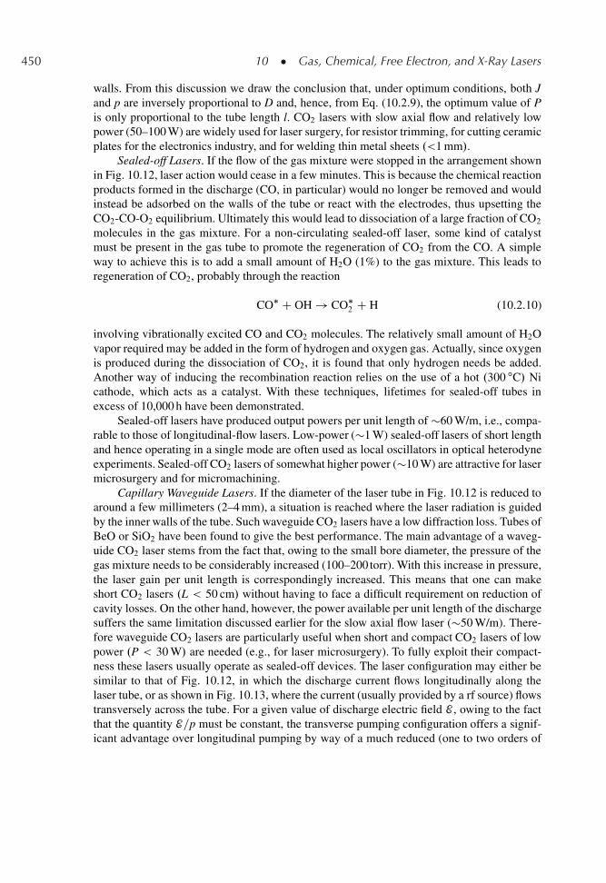
450 10 � Gas, Chemical, Free Electron, and X-Ray Lasers
walls. From this discussion we draw the conclusion that, under optimum conditions, both Jand p are inversely proportional to D and, hence, from Eq. (10.2.9), the optimum value of Pis only proportional to the tube length l. CO2 lasers with slow axial flow and relatively lowpower (50–100 W) are widely used for laser surgery, for resistor trimming, for cutting ceramicplates for the electronics industry, and for welding thin metal sheets .<1 mm/.
Sealed-off Lasers. If the flow of the gas mixture were stopped in the arrangement shownin Fig. 10.12, laser action would cease in a few minutes. This is because the chemical reactionproducts formed in the discharge (CO, in particular) would no longer be removed and wouldinstead be adsorbed on the walls of the tube or react with the electrodes, thus upsetting theCO2-CO-O2 equilibrium. Ultimately this would lead to dissociation of a large fraction of CO2
molecules in the gas mixture. For a non-circulating sealed-off laser, some kind of catalystmust be present in the gas tube to promote the regeneration of CO2 from the CO. A simpleway to achieve this is to add a small amount of H2O (1%) to the gas mixture. This leads toregeneration of CO2, probably through the reaction
CO� C OH ! CO�2 C H (10.2.10)
involving vibrationally excited CO and CO2 molecules. The relatively small amount of H2Ovapor required may be added in the form of hydrogen and oxygen gas. Actually, since oxygenis produced during the dissociation of CO2, it is found that only hydrogen needs be added.Another way of inducing the recombination reaction relies on the use of a hot .300 ıC/ Nicathode, which acts as a catalyst. With these techniques, lifetimes for sealed-off tubes inexcess of 10,000 h have been demonstrated.
Sealed-off lasers have produced output powers per unit length of �60 W/m, i.e., compa-rable to those of longitudinal-flow lasers. Low-power (�1 W) sealed-off lasers of short lengthand hence operating in a single mode are often used as local oscillators in optical heterodyneexperiments. Sealed-off CO2 lasers of somewhat higher power (�10 W) are attractive for lasermicrosurgery and for micromachining.
Capillary Waveguide Lasers. If the diameter of the laser tube in Fig. 10.12 is reduced toaround a few millimeters (2–4 mm), a situation is reached where the laser radiation is guidedby the inner walls of the tube. Such waveguide CO2 lasers have a low diffraction loss. Tubes ofBeO or SiO2 have been found to give the best performance. The main advantage of a waveg-uide CO2 laser stems from the fact that, owing to the small bore diameter, the pressure of thegas mixture needs to be considerably increased (100–200 torr). With this increase in pressure,the laser gain per unit length is correspondingly increased. This means that one can makeshort CO2 lasers .L < 50 cm/ without having to face a difficult requirement on reduction ofcavity losses. On the other hand, however, the power available per unit length of the dischargesuffers the same limitation discussed earlier for the slow axial flow laser (�50 W/m). There-fore waveguide CO2 lasers are particularly useful when short and compact CO2 lasers of lowpower .P < 30 W/ are needed (e.g., for laser microsurgery). To fully exploit their compact-ness these lasers usually operate as sealed-off devices. The laser configuration may either besimilar to that of Fig. 10.12, in which the discharge current flows longitudinally along thelaser tube, or as shown in Fig. 10.13, where the current (usually provided by a rf source) flowstransversely across the tube. For a given value of discharge electric field E , owing to the factthat the quantity E=p must be constant, the transverse pumping configuration offers a signif-icant advantage over longitudinal pumping by way of a much reduced (one to two orders of
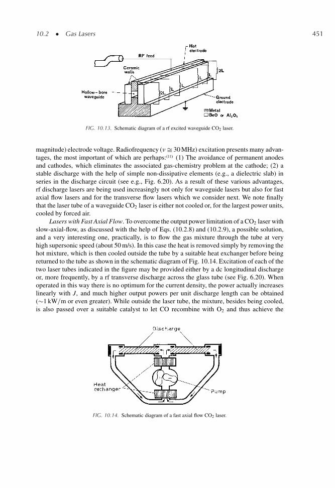
10.2 � Gas Lasers 451
FIG. 10.13. Schematic diagram of a rf excited waveguide CO2 laser.
magnitude) electrode voltage. Radiofrequency (�Š 30 MHz) excitation presents many advan-tages, the most important of which are perhaps:.11/ (1) The avoidance of permanent anodesand cathodes, which eliminates the associated gas-chemistry problem at the cathode; (2) astable discharge with the help of simple non-dissipative elements (e.g., a dielectric slab) inseries in the discharge circuit (see e.g., Fig. 6.20). As a result of these various advantages,rf discharge lasers are being used increasingly not only for waveguide lasers but also for fastaxial flow lasers and for the transverse flow lasers which we consider next. We note finallythat the laser tube of a waveguide CO2 laser is either not cooled or, for the largest power units,cooled by forced air.
Lasers with Fast Axial Flow. To overcome the output power limitation of a CO2 laser withslow-axial-flow, as discussed with the help of Eqs. (10.2.8) and (10.2.9), a possible solution,and a very interesting one, practically, is to flow the gas mixture through the tube at veryhigh supersonic speed (about 50 m/s). In this case the heat is removed simply by removing thehot mixture, which is then cooled outside the tube by a suitable heat exchanger before beingreturned to the tube as shown in the schematic diagram of Fig. 10.14. Excitation of each of thetwo laser tubes indicated in the figure may be provided either by a dc longitudinal dischargeor, more frequently, by a rf transverse discharge across the glass tube (see Fig. 6.20). Whenoperated in this way there is no optimum for the current density, the power actually increaseslinearly with J, and much higher output powers per unit discharge length can be obtained(�1 kW=m or even greater). While outside the laser tube, the mixture, besides being cooled,is also passed over a suitable catalyst to let CO recombine with O2 and thus achieve the
FIG. 10.14. Schematic diagram of a fast axial flow CO2 laser.
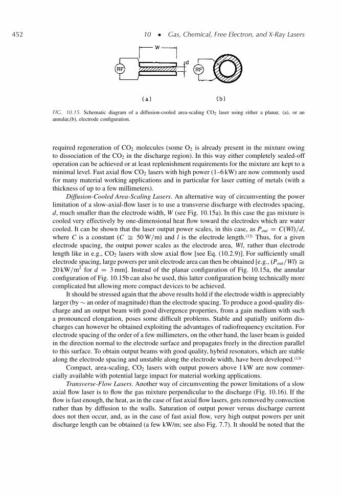
452 10 � Gas, Chemical, Free Electron, and X-Ray Lasers
FIG. 10.15. Schematic diagram of a diffusion-cooled area-scaling CO2 laser using either a planar, (a), or anannular,(b), electrode configuration.
required regeneration of CO2 molecules (some O2 is already present in the mixture owingto dissociation of the CO2 in the discharge region). In this way either completely sealed-offoperation can be achieved or at least replenishment requirements for the mixture are kept to aminimal level. Fast axial flow CO2 lasers with high power (1–6 kW) are now commonly usedfor many material working applications and in particular for laser cutting of metals (with athickness of up to a few millimeters).
Diffusion-Cooled Area-Scaling Lasers. An alternative way of circumventing the powerlimitation of a slow-axial-flow laser is to use a transverse discharge with electrodes spacing,d, much smaller than the electrode width, W (see Fig. 10.15a). In this case the gas mixture iscooled very effectively by one-dimensional heat flow toward the electrodes which are watercooled. It can be shown that the laser output power scales, in this case, as Pout D C.Wl/=d,where C is a constant .C Š 50 W=m/ and l is the electrode length..12/ Thus, for a givenelectrode spacing, the output power scales as the electrode area, Wl, rather than electrodelength like in e.g., CO2 lasers with slow axial flow [see Eq. (10.2.9)]. For sufficiently smallelectrode spacing, large powers per unit electrode area can then be obtained [e.g., .Pout=Wl/ Š20 kW=m2 for d D 3 mm]. Instead of the planar configuration of Fig. 10.15a, the annularconfiguration of Fig. 10.15b can also be used, this latter configuration being technically morecomplicated but allowing more compact devices to be achieved.
It should be stressed again that the above results hold if the electrode width is appreciablylarger (by � an order of magnitude) than the electrode spacing. To produce a good-quality dis-charge and an output beam with good divergence properties, from a gain medium with sucha pronounced elongation, poses some difficult problems. Stable and spatially uniform dis-charges can however be obtained exploiting the advantages of radiofrequency excitation. Forelectrode spacing of the order of a few millimeters, on the other hand, the laser beam is guidedin the direction normal to the electrode surface and propagates freely in the direction parallelto this surface. To obtain output beams with good quality, hybrid resonators, which are stablealong the electrode spacing and unstable along the electrode width, have been developed..13/
Compact, area-scaling, CO2 lasers with output powers above 1 kW are now commer-cially available with potential large impact for material working applications.
Transverse-Flow Lasers. Another way of circumventing the power limitations of a slowaxial flow laser is to flow the gas mixture perpendicular to the discharge (Fig. 10.16). If theflow is fast enough, the heat, as in the case of fast axial flow lasers, gets removed by convectionrather than by diffusion to the walls. Saturation of output power versus discharge currentdoes not then occur, and, as in the case of fast axial flow, very high output powers per unitdischarge length can be obtained (a few kW/m; see also Fig. 7.7). It should be noted that the
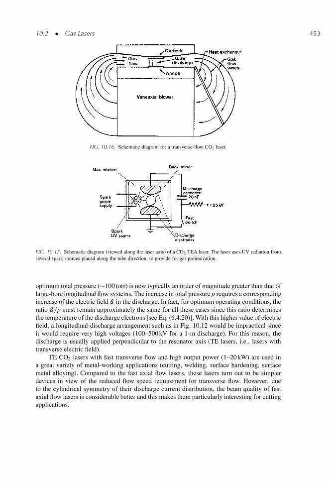
10.2 � Gas Lasers 453
FIG. 10.16. Schematic diagram for a transverse-flow CO2 laser.
FIG. 10.17. Schematic diagram (viewed along the laser axis) of a CO2 TEA laser. The laser uses UV radiation fromseveral spark sources placed along the tube direction, to provide for gas preionization.
optimum total pressure (�100 torr) is now typically an order of magnitude greater than that oflarge-bore longitudinal flow systems. The increase in total pressure p requires a correspondingincrease of the electric field E in the discharge. In fact, for optimum operating conditions, theratio E=p must remain approximately the same for all these cases since this ratio determinesthe temperature of the discharge electrons [see Eq. (6.4.20)]. With this higher value of electricfield, a longitudinal-discharge arrangement such as in Fig. 10.12 would be impractical sinceit would require very high voltages (100–500 kV for a 1-m discharge). For this reason, thedischarge is usually applied perpendicular to the resonator axis (TE lasers, i.e., lasers withtransverse electric field).
TE CO2 lasers with fast transverse flow and high output power (1–20 kW) are used ina great variety of metal-working applications (cutting, welding, surface hardening, surfacemetal alloying). Compared to the fast axial flow lasers, these lasers turn out to be simplerdevices in view of the reduced flow speed requirement for transverse flow. However, dueto the cylindrical symmetry of their discharge current distribution, the beam quality of fastaxial flow lasers is considerable better and this makes them particularly interesting for cuttingapplications.
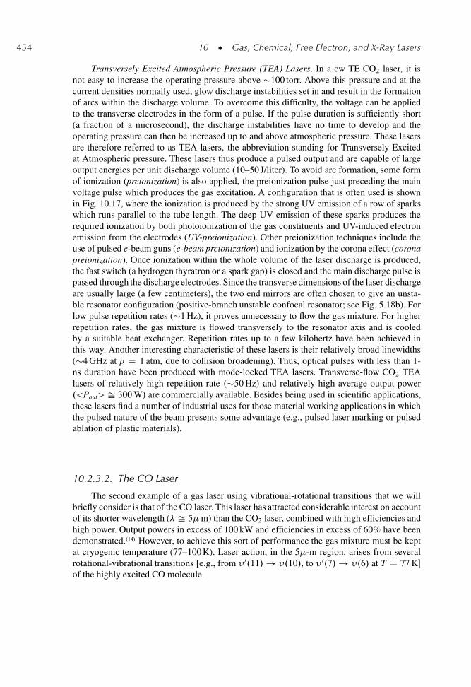
454 10 � Gas, Chemical, Free Electron, and X-Ray Lasers
Transversely Excited Atmospheric Pressure (TEA) Lasers. In a cw TE CO2 laser, it isnot easy to increase the operating pressure above �100 torr. Above this pressure and at thecurrent densities normally used, glow discharge instabilities set in and result in the formationof arcs within the discharge volume. To overcome this difficulty, the voltage can be appliedto the transverse electrodes in the form of a pulse. If the pulse duration is sufficiently short(a fraction of a microsecond), the discharge instabilities have no time to develop and theoperating pressure can then be increased up to and above atmospheric pressure. These lasersare therefore referred to as TEA lasers, the abbreviation standing for Transversely Excitedat Atmospheric pressure. These lasers thus produce a pulsed output and are capable of largeoutput energies per unit discharge volume (10–50 J/liter). To avoid arc formation, some formof ionization (preionization) is also applied, the preionization pulse just preceding the mainvoltage pulse which produces the gas excitation. A configuration that is often used is shownin Fig. 10.17, where the ionization is produced by the strong UV emission of a row of sparkswhich runs parallel to the tube length. The deep UV emission of these sparks produces therequired ionization by both photoionization of the gas constituents and UV-induced electronemission from the electrodes (UV-preionization). Other preionization techniques include theuse of pulsed e-beam guns (e-beam preionization) and ionization by the corona effect (coronapreionization). Once ionization within the whole volume of the laser discharge is produced,the fast switch (a hydrogen thyratron or a spark gap) is closed and the main discharge pulse ispassed through the discharge electrodes. Since the transverse dimensions of the laser dischargeare usually large (a few centimeters), the two end mirrors are often chosen to give an unsta-ble resonator configuration (positive-branch unstable confocal resonator; see Fig. 5.18b). Forlow pulse repetition rates (�1 Hz), it proves unnecessary to flow the gas mixture. For higherrepetition rates, the gas mixture is flowed transversely to the resonator axis and is cooledby a suitable heat exchanger. Repetition rates up to a few kilohertz have been achieved inthis way. Another interesting characteristic of these lasers is their relatively broad linewidths(�4 GHz at p D 1 atm, due to collision broadening). Thus, optical pulses with less than 1-ns duration have been produced with mode-locked TEA lasers. Transverse-flow CO2 TEAlasers of relatively high repetition rate .�50 Hz/ and relatively high average output power.<Pout> Š 300 W/ are commercially available. Besides being used in scientific applications,these lasers find a number of industrial uses for those material working applications in whichthe pulsed nature of the beam presents some advantage (e.g., pulsed laser marking or pulsedablation of plastic materials).
10.2.3.2. The CO Laser
The second example of a gas laser using vibrational-rotational transitions that we willbriefly consider is that of the CO laser. This laser has attracted considerable interest on accountof its shorter wavelength (� Š 5�m) than the CO2 laser, combined with high efficiencies andhigh power. Output powers in excess of 100 kW and efficiencies in excess of 60% have beendemonstrated..14/ However, to achieve this sort of performance the gas mixture must be keptat cryogenic temperature (77–100 K). Laser action, in the 5�-m region, arises from severalrotational-vibrational transitions [e.g., from � 0.11/ ! �.10/, to � 0.7/ ! �.6/ at T D 77 K�of the highly excited CO molecule.
10.2 � Gas Lasers 455
FIG. 10.18. Partial inversion between two vibrational transitions (� and � 0) having the same total population.
Pumping of the CO vibrational levels is achieved by electron-impact excitation. Likethe isoelectronic N2 molecule, the CO molecule has an unusually large cross section forelectron-impact excitation of its vibrational levels. Thus, nearly 90% of the electron energyin a discharge can be converted into vibrational energy of CO molecules. Another impor-tant feature of the CO molecule is that VV relaxation proceeds at a much faster rate thanVT relaxation (which is unusually low). As a consequence of this, a non-Boltzmann pop-ulation buildup in higher vibrational levels, by a process known as anharmonic pumping,plays a very important role�. Although this phenomenon does not allow a total inversionin the vibrational population of a CO molecule, a situation known as partial inversion mayoccur. This is illustrated in Fig. 10.18, in which the rotational populations of two neigh-boring vibrational states are indicated. One sees from the figure that, although the totalpopulation for the two vibrational states is equal, an inversion exists for the two P transi-tions Œ.J0 D 5/ ! .J D 6/, .J0 D 4/ ! .J D 5/� and also for the two R-branch transitionsindicated in the figure. Under these conditions of partial inversion, laser action can thus takeplace, and a new phenomenon, called cascading, can then play an important role. The effectof laser action is in fact to depopulate a rotational level of the upper state and populate arotational level of the lower vibrational state. The latter level can then accumulate enoughpopulation to result in population inversion with respect to a rotational level of a still lowervibrational state. At the same time, the rotational level of the upper state may become suf-ficiently depopulated to result in population inversion with respect to a rotational level of astill higher vibrational state. This process of cascading coupled with the very low VT rateresults in most of the vibrational energy being extracted as laser output energy. This, togetherwith the very high excitation efficiency, accounts for the high efficiency of the CO laser. Thelow-temperature requirement arises from the need for very efficient anharmonic pumping. In
� Anharmonic pumping arises from a collision of the type CO.� D n/CCO.� D m/ ! CO.� D nC1/CCO.� Dm � 1/ with n > m. Because of anharmonicity (a phenomenon shown by all molecular oscillators), the separationbetween vibrational levels becomes smaller for levels higher up in the vibrational ladder (see also Fig. 3.1). Thismeans that, in a collision process of the type indicated above, with n > m, the total vibrational energy of thetwo CO molecules after collision is somewhat smaller than before collision. The collision process therefore has agreater probability of proceeding in this direction rather than the reverse direction. This means that the hottest COmolecule ŒCO.� D n/� can climb up the vibrational ladder and this leads to a non-Boltzmann distribution of thepopulation among the vibrational levels.
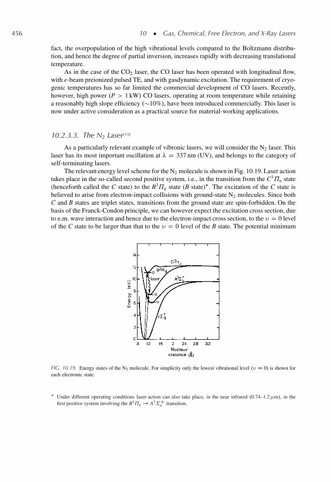
456 10 � Gas, Chemical, Free Electron, and X-Ray Lasers
fact, the overpopulation of the high vibrational levels compared to the Boltzmann distribu-tion, and hence the degree of partial inversion, increases rapidly with decreasing translationaltemperature.
As in the case of the CO2 laser, the CO laser has been operated with longitudinal flow,with e-beam preionized pulsed TE, and with gasdynamic excitation. The requirement of cryo-genic temperatures has so far limited the commercial development of CO lasers. Recently,however, high power .P > 1 kW/ CO lasers, operating at room temperature while retaininga reasonably high slope efficiency .�10%/, have been introduced commercially. This laser isnow under active consideration as a practical source for material-working applications.
10.2.3.3. The N2 Laser.15/
As a particularly relevant example of vibronic lasers, we will consider the N2 laser. Thislaser has its most important oscillation at � D 337 nm (UV), and belongs to the category ofself-terminating lasers.
The relevant energy level scheme for the N2 molecule is shown in Fig. 10.19. Laser actiontakes place in the so-called second positive system, i.e., in the transition from the C3˘u state(henceforth called the C state) to the B3˘g state (B state)�. The excitation of the C state isbelieved to arise from electron-impact collisions with ground-state N2 molecules. Since bothC and B states are triplet states, transitions from the ground state are spin-forbidden. On thebasis of the Franck-Condon principle, we can however expect the excitation cross section, dueto e.m. wave interaction and hence due to the electron-impact cross section, to the � D 0 levelof the C state to be larger than that to the � D 0 level of the B state. The potential minimum
FIG. 10.19. Energy states of the N2 molecule. For simplicity only the lowest vibrational level .� D 0/ is shown foreach electronic state.
� Under different operating conditions laser action can also take place, in the near infrared .0.74–1.2�m/, in thefirst positive system involving the B3˘g ! A3˙C
u transition.
10.2 � Gas Lasers 457
TABLE 10.2. Spectroscopic properties of UV laser transitions and gas-mixture composition in nitrogenand KrF lasers
Laser type N2 .KrF/�
Laser wavelength [nm] 337.1 248Cross-section Œ10�14 cm2� 40 0.05Upper-state lifetime [ns] 40 10Lower-state lifetime [ns] 10 sTransition Linewidth [THz] 0.25 3Partial press. of gas mixture [mbar] 40 (N2) 120 (Kr)
960 (He) 6 .F2/
2,400 (He)
of the B state is in fact shifted (relative to the ground state) to larger internuclear separationthan that of the C state. The lifetime (radiative) of the C state is 40 ns, while the lifetime ofthe B state is 10� s. Clearly the laser cannot operate cw since condition Eq. (7.3.1) is notsatisfied. The laser can, however, be excited on a pulsed basis provided the electrical pulse isappreciably shorter than 40 ns. Laser action takes place predominantly on several rotationallines of the � 00.0/ ! � 0.0/ transition .� D 337.1 nm/ because this transition exhibits thelargest stimulated-emission cross-section. Oscillation on the � 00.1/ ! � 0.0/.� D 357.7 nm/transition and the � 00.0/ ! � 0.1/.� D 315.9 nm/ transition also occurs, although with lowerintensity. Some spectroscopic data for the N2 laser are summarized in Table 10.2.
Given the high pressure of the gas mixture (�40 mbar of N2 and 960 mbar of He) andthe correspondingly high electric field (�10 kV/cm), a TEA configuration (see Fig. 10.17)is normally used for a nitrogen laser. To obtain the required fast current pulse (5–10 ns), thedischarge circuit must have as low an inductance as possible. Owing to the high gain of thisself-terminating transition, oscillation takes place in the form of amplified spontaneous emis-sion (ASE) and the laser can be operated even without mirrors. Usually, however, a singlemirror is placed at one end of the laser since this reduces the threshold gain and hence thethreshold electrical energy for ASE emission (see Sect. 2.9.2). The mirror also ensures a uni-directional output and reduces the beam divergence. With this type of laser, it is possible toobtain laser pulses, of high peak power (up to �1 MW) and short duration (�10 ns), at highrepetition rate (up to �100 Hz). Nitrogen lasers with nitrogen pressure up to atmosphericpressure and without helium have also been developed. In this case, the problem of arcing isalleviated by further reducing (to �1 ns) the duration of the voltage pulse. The increased gainper unit length, due to the higher N2 pressure, and the fast discharge, leads to this type of laserusually being operated without any mirrors. The length can be kept very short (10–50 cm)and, as a consequence, output pulses of shorter time duration can be obtained (�100 ps with100 kW peak power). Nitrogen lasers of both long (�10 ns) and short (�100 ps) time durationare widely used as pumps for dye lasers, since most dyes absorb strongly in the UV.
10.2.3.4. Excimer Lasers.17/
Excimer lasers represent an interesting and important class of molecular lasers involvingtransitions between different electronic states of special molecules referred to as excimers.Consider a diatomic molecule A2 with potential energy curves as in Fig. 10.20, for the ground
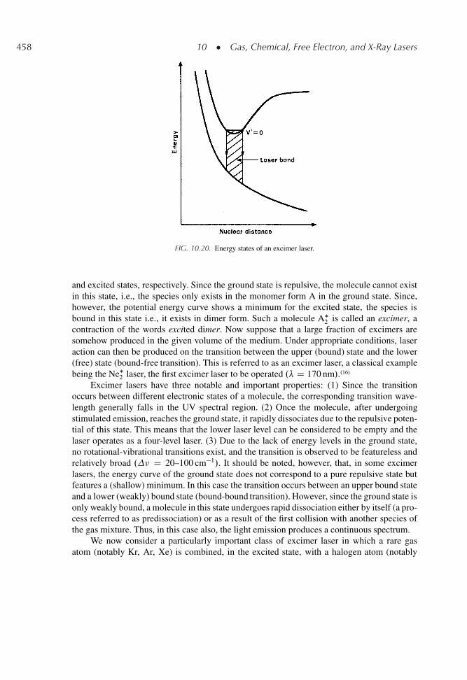
458 10 � Gas, Chemical, Free Electron, and X-Ray Lasers
FIG. 10.20. Energy states of an excimer laser.
and excited states, respectively. Since the ground state is repulsive, the molecule cannot existin this state, i.e., the species only exists in the monomer form A in the ground state. Since,however, the potential energy curve shows a minimum for the excited state, the species isbound in this state i.e., it exists in dimer form. Such a molecule A�
2 is called an excimer, acontraction of the words excited dimer. Now suppose that a large fraction of excimers aresomehow produced in the given volume of the medium. Under appropriate conditions, laseraction can then be produced on the transition between the upper (bound) state and the lower(free) state (bound-free transition). This is referred to as an excimer laser, a classical examplebeing the Ne�
2 laser, the first excimer laser to be operated .� D 170 nm/..16/
Excimer lasers have three notable and important properties: (1) Since the transitionoccurs between different electronic states of a molecule, the corresponding transition wave-length generally falls in the UV spectral region. (2) Once the molecule, after undergoingstimulated emission, reaches the ground state, it rapidly dissociates due to the repulsive poten-tial of this state. This means that the lower laser level can be considered to be empty and thelaser operates as a four-level laser. (3) Due to the lack of energy levels in the ground state,no rotational-vibrational transitions exist, and the transition is observed to be featureless andrelatively broad .� D 20–100 cm�1/. It should be noted, however, that, in some excimerlasers, the energy curve of the ground state does not correspond to a pure repulsive state butfeatures a (shallow) minimum. In this case the transition occurs between an upper bound stateand a lower (weakly) bound state (bound-bound transition). However, since the ground state isonly weakly bound, a molecule in this state undergoes rapid dissociation either by itself (a pro-cess referred to as predissociation) or as a result of the first collision with another species ofthe gas mixture. Thus, in this case also, the light emission produces a continuous spectrum.
We now consider a particularly important class of excimer laser in which a rare gasatom (notably Kr, Ar, Xe) is combined, in the excited state, with a halogen atom (notably
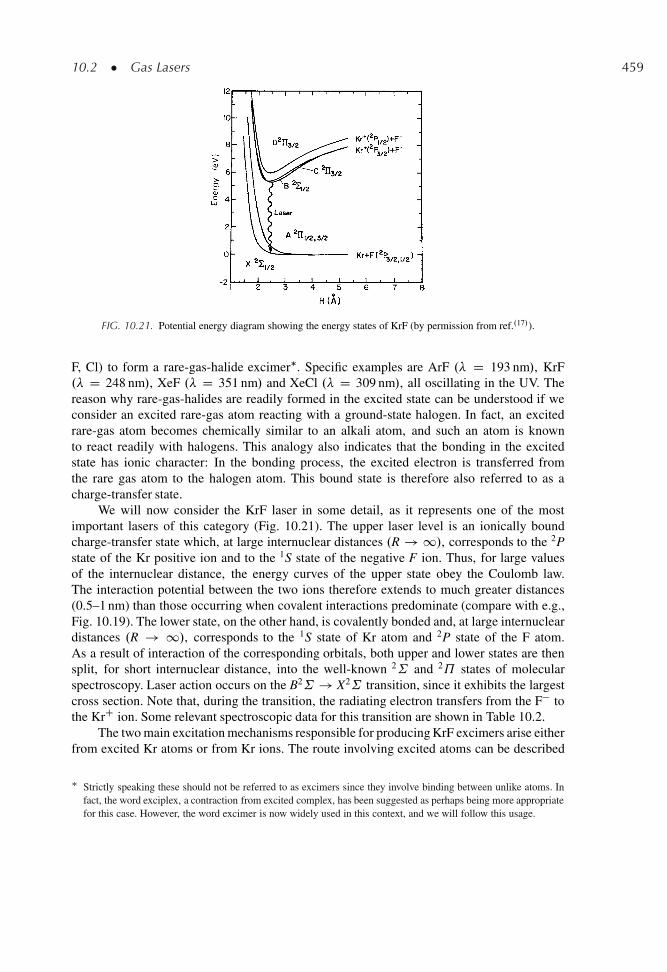
10.2 � Gas Lasers 459
FIG. 10.21. Potential energy diagram showing the energy states of KrF (by permission from ref..17/).
F, Cl) to form a rare-gas-halide excimer�. Specific examples are ArF .� D 193 nm/, KrF.� D 248 nm/, XeF .� D 351 nm/ and XeCl .� D 309 nm/, all oscillating in the UV. Thereason why rare-gas-halides are readily formed in the excited state can be understood if weconsider an excited rare-gas atom reacting with a ground-state halogen. In fact, an excitedrare-gas atom becomes chemically similar to an alkali atom, and such an atom is knownto react readily with halogens. This analogy also indicates that the bonding in the excitedstate has ionic character: In the bonding process, the excited electron is transferred fromthe rare gas atom to the halogen atom. This bound state is therefore also referred to as acharge-transfer state.
We will now consider the KrF laser in some detail, as it represents one of the mostimportant lasers of this category (Fig. 10.21). The upper laser level is an ionically boundcharge-transfer state which, at large internuclear distances .R ! 1/, corresponds to the 2Pstate of the Kr positive ion and to the 1S state of the negative F ion. Thus, for large valuesof the internuclear distance, the energy curves of the upper state obey the Coulomb law.The interaction potential between the two ions therefore extends to much greater distances(0.5–1 nm) than those occurring when covalent interactions predominate (compare with e.g.,Fig. 10.19). The lower state, on the other hand, is covalently bonded and, at large internucleardistances .R ! 1/, corresponds to the 1S state of Kr atom and 2P state of the F atom.As a result of interaction of the corresponding orbitals, both upper and lower states are thensplit, for short internuclear distance, into the well-known 2˙ and 2˘ states of molecularspectroscopy. Laser action occurs on the B2˙ ! X2˙ transition, since it exhibits the largestcross section. Note that, during the transition, the radiating electron transfers from the F� tothe KrC ion. Some relevant spectroscopic data for this transition are shown in Table 10.2.
The two main excitation mechanisms responsible for producing KrF excimers arise eitherfrom excited Kr atoms or from Kr ions. The route involving excited atoms can be described
� Strictly speaking these should not be referred to as excimers since they involve binding between unlike atoms. Infact, the word exciplex, a contraction from excited complex, has been suggested as perhaps being more appropriatefor this case. However, the word excimer is now widely used in this context, and we will follow this usage.
460 10 � Gas, Chemical, Free Electron, and X-Ray Lasers
by the following reactions
e C Kr ! e C Kr� (10.2.11a)
Kr� C F2 ! .KrF/� C F (10.2.11b)
where Kr is first excited by a discharge electron and then reacts with a fluorine molecule. Theroute involving Kr ions, on the other hand, can be described by the following three reactions
e C Kr ! 2e C KrC (10.2.12a)
e C F2 ! F� C F (10.2.12b)
F� C KrC C M ! .KrF/� C M (10.2.12c)
involving first production of Kr and F ions and then their recombination, in the dischargevolume, in the presence of a third partner (usually He, referred to as a buffer gas), to satisfyboth energy and momentum conservation. Note that reaction Eq. (10.2.12b) is a peculiar one,usually referred to as dissociative attachment, resulting from the high electron affinity of Fatoms. Note also that, due to the long-range interaction between the two reacting ions, thereaction Eq. (10.2.12c) can proceed at very fast rate provided that the buffer gas pressure issufficiently high. Indeed, He partial pressures well above atmospheric pressure are normallyused (a typical gas mixture may contain �120 mbar of Kr, 6 mbar of F2 and 2,400 mbar of He).Under this condition, the reaction pathway described by Eqs. (10.2.12) becomes the dominantmechanism of .KrF/� production.
Since the pressure of the gas mixture is above atmospheric pressure, excimer lasers canonly be operated in a pulsed regime and the general TEA configuration of Fig. 10.17 is used.In the case of excimer lasers, however, the components of the laser tube and laser flow systemmust be compatible with the highly reactive F2 gas. Furthermore, owing to the shorter lifetimeof the upper state and to avoid the onset of arc formation, faster pumping is usually providedfor excimer lasers compared to TEA CO2 lasers (pump durations of 10–20 ns are typical). Forstandard systems, preionization is achieved, as in Fig. 10.17, by a row of sparks. However,for the largest systems, more complex preionization arrangements are adopted, using eitheran auxiliary electron-beam or an X-ray source.
Excimer lasers with high repetition rate (up to �500 Hz) and high average power (upto �100 W) are commercially available, while larger, laboratory, systems exist with higheraverage power (in excess of a few kW). The efficiency of these lasers is usually quite high(2–4%) as a result of the high quantum efficiency (see Fig. 10.21) and the high efficiency ofthe pumping processes.
Excimer lasers are used to ablate plastic as well as biological materials with great preci-sion since these material exhibit strong absorption at UV wavelengths. In fact, in some of thesematerials, the penetration depth, for each laser pulse, may be only a few�m. Due to the strongabsorption and short pulse duration, a violent ablation process is produced wherein thesematerials are directly transformed into volatile components. Applications include drillingof very precise holes in thin plastic films (as used e.g., for the ink-jet printer head) andcorneal sculpturing to change the refractive power of the eye and hence correct myopia. Inthe field of lithography, the 193 nm UV light provides a good illumination source for achiev-ing submicron-size features in semiconductor microchips. Excimer lasers can also be used asdye-laser pumps since most dye absorb strongly in the UV.
10.3 � Chemical Lasers 461
10.3. CHEMICAL LASERS.18,19/
A chemical laser is usually defined as one in which the population inversion is “directly”produced by an exothermic chemical reaction�. Chemical lasers usually involve either anassociative or a dissociative chemical reaction between gaseous elements.
An associative reaction can be described by an equation of the form A CB ! AB. For anexothermic reaction, some of the heat of reaction will appear as either rotational-vibrationalor electronic energy of the molecule AB. Thus, if a population inversion is achieved, the asso-ciative reaction can in principle lead to either a vibrational-rotational or a vibronic transition.In spite of much effort, however, only chemical lasers operating on vibrational-rotationaltransitions have been demonstrated so far. For this kind of transition, the range of oscilla-tion wavelengths, achieved so far, lies between 3 and 10�m, with the HF and DF lasers,considered in the next section, being the most notable examples.
A dissociative reaction, on the other hand, can be described by an equation of the generalform ABC ! A C BC. If the reaction is exothermic, some of the heat of reaction can be lefteither as electronic energy of the atomic species A or as internal energy of the molecularspecies BC. The most notable example of a laser exploiting this type of reaction is the atomiciodine laser, in which iodine is chemically excited to its 2P1=2 state and laser action occursbetween the 2P1=2 state and the 2P3=2 ground state .� D 1.315�m/. Excited atomic iodinemay be produced via the exothermic dissociation of CH3I (or CF3I, C3F7I), the dissociationbeing produced by means of UV light .�300 nm/ from powerful flashlamps. More recently,excited iodine has been produced via generation of excited molecular oxygen by reactingmolecular chlorine with hydrogen peroxide. The molecular oxygen, excited to its long-livedsinglet-state (the ground electronic state of oxygen molecule happens in fact to be a tripletstate), in turn transfers its energy to atomic iodine (oxygen-iodine chemical laser).
Chemical lasers are important mainly for two main reasons: (1) They provide an interest-ing example of direct conversion of chemical energy into electromagnetic energy. (2) They arepotentially able to provide either high output power (in cw operation) or high output energy (inpulsed operation). This is because the amount of energy available in an exothermic chemicalreaction is usually quite large�.
10.3.1. The HF Laser
HF chemical lasers can be operated using either SF6 or F2 as compounds donating theatomic fluorine, and, from a practical view-point, the two lasers are very different. In commer-cial devices, the inert SF6 molecule is used as fluorine donor and the gas mixture also containsH2 and a large amount of He. An electrical discharge is then used to dissociate the SF6 andexcite the reaction. The overall pressure of the mixture is around atmospheric pressure, the
� According to this definition, the gas-dynamic CO2 laser, briefly considered in Sect. 6.1., should not be regarded asa chemical laser even though the upper state population arises ultimately from a combustion reaction.
� For example, a mixture of H2, F2, and other substances (16% of H2 and F2 in a gas mixture at atmosphericpressure) has a heat of reaction equal to 2,000 J/liter, of which 1,000 J is left as vibrational energy of HF (a largevalue in terms of available laser energy).
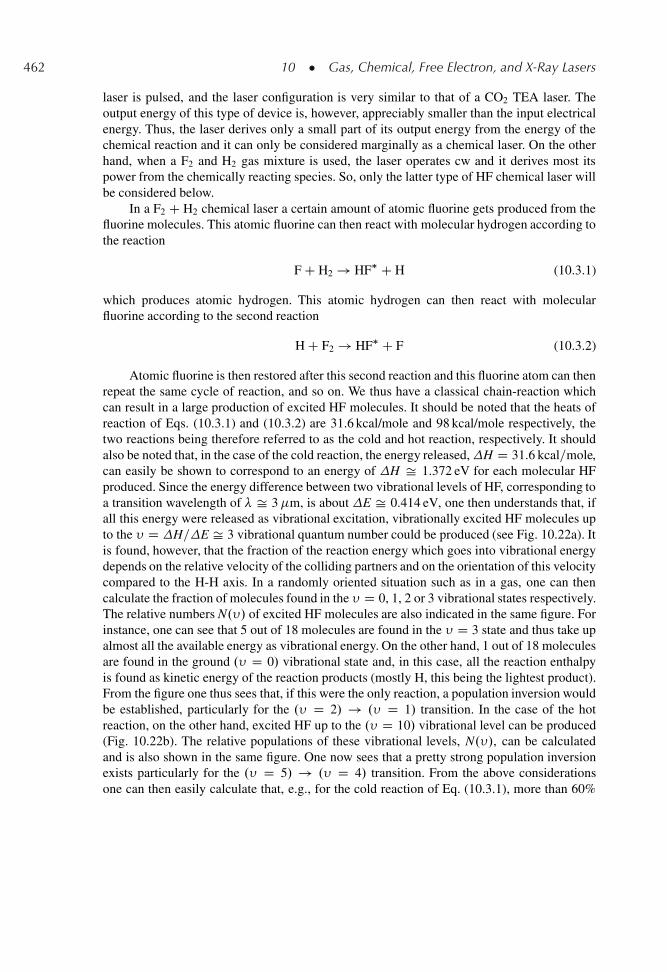
462 10 � Gas, Chemical, Free Electron, and X-Ray Lasers
laser is pulsed, and the laser configuration is very similar to that of a CO2 TEA laser. Theoutput energy of this type of device is, however, appreciably smaller than the input electricalenergy. Thus, the laser derives only a small part of its output energy from the energy of thechemical reaction and it can only be considered marginally as a chemical laser. On the otherhand, when a F2 and H2 gas mixture is used, the laser operates cw and it derives most itspower from the chemically reacting species. So, only the latter type of HF chemical laser willbe considered below.
In a F2 C H2 chemical laser a certain amount of atomic fluorine gets produced from thefluorine molecules. This atomic fluorine can then react with molecular hydrogen according tothe reaction
F C H2 ! HF� C H (10.3.1)
which produces atomic hydrogen. This atomic hydrogen can then react with molecularfluorine according to the second reaction
H C F2 ! HF� C F (10.3.2)
Atomic fluorine is then restored after this second reaction and this fluorine atom can thenrepeat the same cycle of reaction, and so on. We thus have a classical chain-reaction whichcan result in a large production of excited HF molecules. It should be noted that the heats ofreaction of Eqs. (10.3.1) and (10.3.2) are 31.6 kcal/mole and 98 kcal/mole respectively, thetwo reactions being therefore referred to as the cold and hot reaction, respectively. It shouldalso be noted that, in the case of the cold reaction, the energy released,H D 31.6 kcal=mole,can easily be shown to correspond to an energy of H Š 1.372 eV for each molecular HFproduced. Since the energy difference between two vibrational levels of HF, corresponding toa transition wavelength of � Š 3�m, is about E Š 0.414 eV, one then understands that, ifall this energy were released as vibrational excitation, vibrationally excited HF molecules upto the � D H=E Š 3 vibrational quantum number could be produced (see Fig. 10.22a). Itis found, however, that the fraction of the reaction energy which goes into vibrational energydepends on the relative velocity of the colliding partners and on the orientation of this velocitycompared to the H-H axis. In a randomly oriented situation such as in a gas, one can thencalculate the fraction of molecules found in the � D 0, 1, 2 or 3 vibrational states respectively.The relative numbers N.�/ of excited HF molecules are also indicated in the same figure. Forinstance, one can see that 5 out of 18 molecules are found in the � D 3 state and thus take upalmost all the available energy as vibrational energy. On the other hand, 1 out of 18 moleculesare found in the ground .� D 0/ vibrational state and, in this case, all the reaction enthalpyis found as kinetic energy of the reaction products (mostly H, this being the lightest product).From the figure one thus sees that, if this were the only reaction, a population inversion wouldbe established, particularly for the .� D 2/ ! .� D 1/ transition. In the case of the hotreaction, on the other hand, excited HF up to the .� D 10/ vibrational level can be produced(Fig. 10.22b). The relative populations of these vibrational levels, N.�/, can be calculatedand is also shown in the same figure. One now sees that a pretty strong population inversionexists particularly for the .� D 5/ ! .� D 4/ transition. From the above considerationsone can then easily calculate that, e.g., for the cold reaction of Eq. (10.3.1), more than 60%
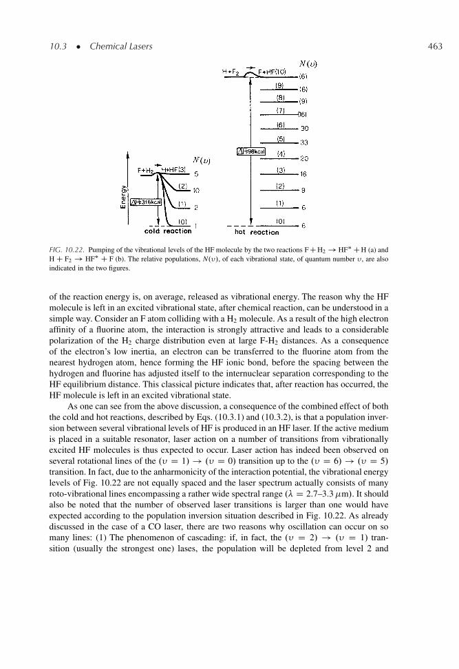
10.3 � Chemical Lasers 463
FIG. 10.22. Pumping of the vibrational levels of the HF molecule by the two reactions F C H2 ! HF� C H (a) andH C F2 ! HF� C F (b). The relative populations, N.�/, of each vibrational state, of quantum number � , are alsoindicated in the two figures.
of the reaction energy is, on average, released as vibrational energy. The reason why the HFmolecule is left in an excited vibrational state, after chemical reaction, can be understood in asimple way. Consider an F atom colliding with a H2 molecule. As a result of the high electronaffinity of a fluorine atom, the interaction is strongly attractive and leads to a considerablepolarization of the H2 charge distribution even at large F-H2 distances. As a consequenceof the electron’s low inertia, an electron can be transferred to the fluorine atom from thenearest hydrogen atom, hence forming the HF ionic bond, before the spacing between thehydrogen and fluorine has adjusted itself to the internuclear separation corresponding to theHF equilibrium distance. This classical picture indicates that, after reaction has occurred, theHF molecule is left in an excited vibrational state.
As one can see from the above discussion, a consequence of the combined effect of boththe cold and hot reactions, described by Eqs. (10.3.1) and (10.3.2), is that a population inver-sion between several vibrational levels of HF is produced in an HF laser. If the active mediumis placed in a suitable resonator, laser action on a number of transitions from vibrationallyexcited HF molecules is thus expected to occur. Laser action has indeed been observed onseveral rotational lines of the .� D 1/ ! .� D 0/ transition up to the .� D 6/ ! .� D 5/transition. In fact, due to the anharmonicity of the interaction potential, the vibrational energylevels of Fig. 10.22 are not equally spaced and the laser spectrum actually consists of manyroto-vibrational lines encompassing a rather wide spectral range .� D 2.7–3.3�m/. It shouldalso be noted that the number of observed laser transitions is larger than one would haveexpected according to the population inversion situation described in Fig. 10.22. As alreadydiscussed in the case of a CO laser, there are two reasons why oscillation can occur on somany lines: (1) The phenomenon of cascading: if, in fact, the .� D 2/ ! .� D 1/ tran-sition (usually the strongest one) lases, the population will be depleted from level 2 and
464 10 � Gas, Chemical, Free Electron, and X-Ray Lasers
FIG. 10.23. Supersonic-diffusion HF (or DF) chemical laser (after ref..18/).
will accumulate in level 1. Consequently, laser action on the .� D 3/ ! .� D 2/ and.� D 1/ ! .� D 0/ transition now become more favored. (2) The phenomenon of partialinversion, according to which there may be a population inversion between some rotationallines even when no inversion exists between the overall populations of the correspondingvibrational levels. Finally, it should be noted that, besides laser action in HF, laser action canalso be achieved in the analogous compounds DF, HCl, and HBr thus providing oscillation ona large number of transitions in the 3.5–5�m range.
A possible configuration for a high-power cw HF or DF laser is shown in Fig. 10.23.Fluorine is thermally dissociated by an arc jet heater and then expanded to supersonic veloc-ity .� Mach 4/ through some appropriate expansion nozzles. Molecular hydrogen is thenmixed downstream through some appropriate perforated tubes inserted in the nozzles. Down-stream in the expansion regions, excited HF molecules are produced by the chain reactionsEqs. (10.3.1) and (10.3.2) and a suitable resonator, with its axis orthogonal to the flow direc-tion, is placed around this region. To handle the large power available in the expanding beam,usually of large diameter, unstable resonators exploiting metallic water-cooled mirror areoften utilized. Chemical lasers of this type can produce very large c.w. output powers (inthe MW range!) with good chemical efficiency.
Pulsed TEA type HF lasers are commercially available and have found a limited usewhen an intense source of middle infrared radiation is needed (e.g., in spectroscopy). HF andDF chemical lasers of the type described in Fig. 10.23 are used exclusively for military appli-cations. Safety considerations have indeed prevented the use of these lasers for commercialapplications. In fact, the F2 molecule is one of the most corrosive and reactive element known,the waste products are difficult to dispose of, and, under certain conditions, the chain reactionEqs. (10.3.1) and (10.3.2) may even become explosive. In the military field, due to the largeavailable output powers, these lasers can be used as directed energy weapons to e.g., destroyenemy missiles. A military c.w. device named MIRACL (Mid-Infrared Advanced ChemicalLaser), using DF, has given the largest c.w. power of any laser (2.2 MW). DF rather thanHF molecule was used because the system was intended for use from a ground station andthe DF emission wavelengths fall in a region of relatively good atmospheric transmission.More recently, HF lasers of somewhat higher power .�5 MW/ have been constructed. Thelaser is intended to be used either from a high altitude plane, for destruction of missile duringtheir ballistic flight, or from a space station, for missile destruction during their lift-off phase(where the rocket has much lower speed and hence is much more vulnerable).
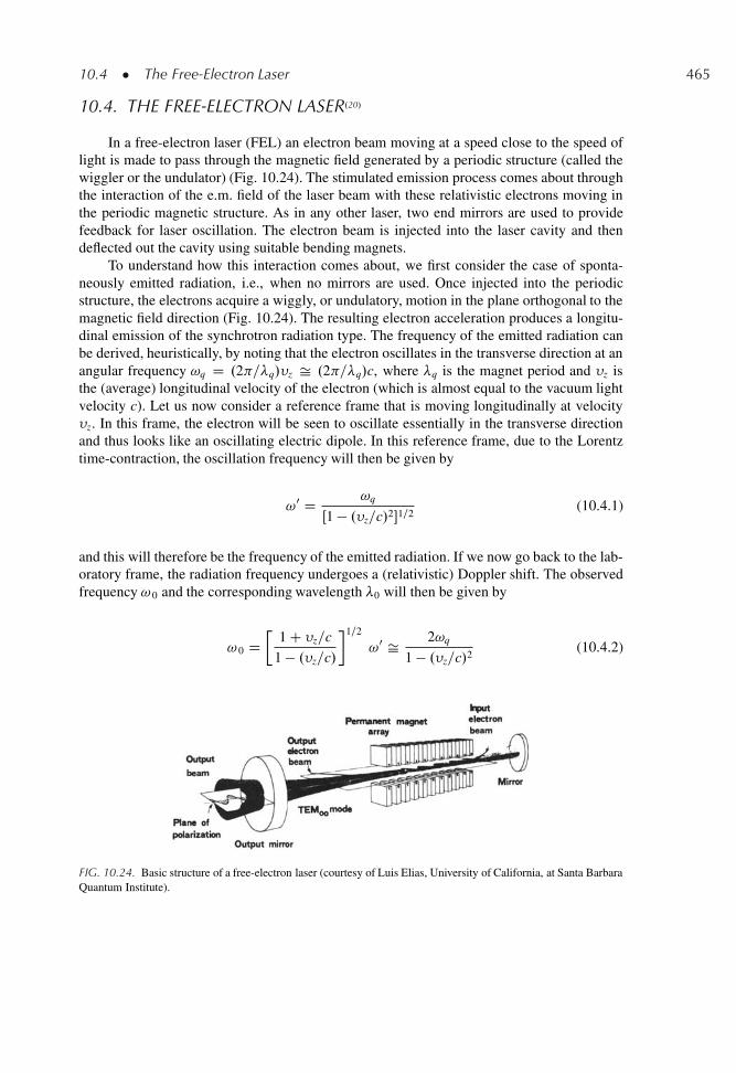
10.4 � The Free-Electron Laser 465
10.4. THE FREE-ELECTRON LASER.20/
In a free-electron laser (FEL) an electron beam moving at a speed close to the speed oflight is made to pass through the magnetic field generated by a periodic structure (called thewiggler or the undulator) (Fig. 10.24). The stimulated emission process comes about throughthe interaction of the e.m. field of the laser beam with these relativistic electrons moving inthe periodic magnetic structure. As in any other laser, two end mirrors are used to providefeedback for laser oscillation. The electron beam is injected into the laser cavity and thendeflected out the cavity using suitable bending magnets.
To understand how this interaction comes about, we first consider the case of sponta-neously emitted radiation, i.e., when no mirrors are used. Once injected into the periodicstructure, the electrons acquire a wiggly, or undulatory, motion in the plane orthogonal to themagnetic field direction (Fig. 10.24). The resulting electron acceleration produces a longitu-dinal emission of the synchrotron radiation type. The frequency of the emitted radiation canbe derived, heuristically, by noting that the electron oscillates in the transverse direction at anangular frequency !q D .2 =�q/�z Š .2 =�q/c, where �q is the magnet period and �z isthe (average) longitudinal velocity of the electron (which is almost equal to the vacuum lightvelocity c). Let us now consider a reference frame that is moving longitudinally at velocity�z. In this frame, the electron will be seen to oscillate essentially in the transverse directionand thus looks like an oscillating electric dipole. In this reference frame, due to the Lorentztime-contraction, the oscillation frequency will then be given by
!0 D !q
Œ1 � .�z=c/2�1=2(10.4.1)
and this will therefore be the frequency of the emitted radiation. If we now go back to the lab-oratory frame, the radiation frequency undergoes a (relativistic) Doppler shift. The observedfrequency ! 0 and the corresponding wavelength �0 will then be given by
! 0 D�
1 C �z=c
1 � .�z=c/
�1=2
!0 Š 2!q
1 � .�z=c/2(10.4.2)
FIG. 10.24. Basic structure of a free-electron laser (courtesy of Luis Elias, University of California, at Santa BarbaraQuantum Institute).
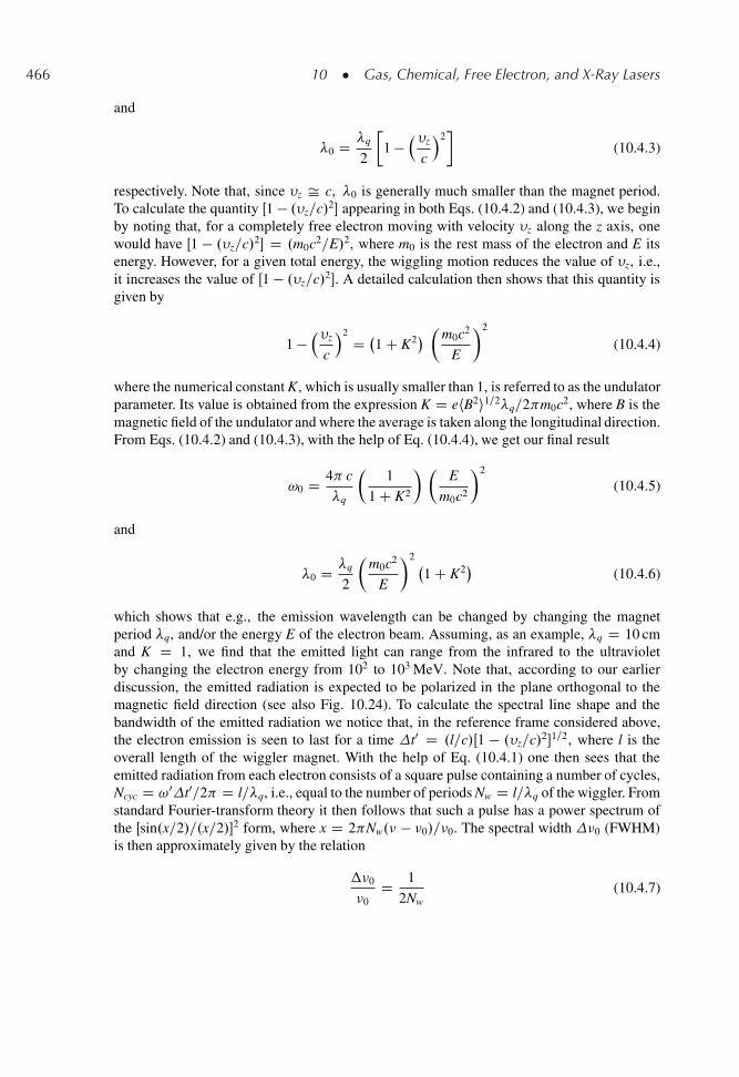
466 10 � Gas, Chemical, Free Electron, and X-Ray Lasers
and
�0 D �q
2
�1 �
��z
c
�2�
(10.4.3)
respectively. Note that, since �z Š c, �0 is generally much smaller than the magnet period.To calculate the quantity Œ1 � .�z=c/2� appearing in both Eqs. (10.4.2) and (10.4.3), we beginby noting that, for a completely free electron moving with velocity �z along the z axis, onewould have Œ1 � .�z=c/2� D .m0c2=E/2, where m0 is the rest mass of the electron and E itsenergy. However, for a given total energy, the wiggling motion reduces the value of �z, i.e.,it increases the value of Œ1 � .�z=c/2�. A detailed calculation then shows that this quantity isgiven by
1 ���z
c
�2 D 1 C K2� �m0c2
E
�2
(10.4.4)
where the numerical constant K, which is usually smaller than 1, is referred to as the undulatorparameter. Its value is obtained from the expression K D ehB2i1=2�q=2 m0c2, where B is themagnetic field of the undulator and where the average is taken along the longitudinal direction.From Eqs. (10.4.2) and (10.4.3), with the help of Eq. (10.4.4), we get our final result
!0 D 4 c
�q
�1
1 C K2
� �E
m0c2
�2
(10.4.5)
and
�0 D �q
2
�m0c2
E
�2 1 C K2
�(10.4.6)
which shows that e.g., the emission wavelength can be changed by changing the magnetperiod �q, and/or the energy E of the electron beam. Assuming, as an example, �q D 10 cmand K D 1, we find that the emitted light can range from the infrared to the ultravioletby changing the electron energy from 102 to 103 MeV. Note that, according to our earlierdiscussion, the emitted radiation is expected to be polarized in the plane orthogonal to themagnetic field direction (see also Fig. 10.24). To calculate the spectral line shape and thebandwidth of the emitted radiation we notice that, in the reference frame considered above,the electron emission is seen to last for a time t0 D .l=c/Œ1 � .�z=c/2�1=2, where l is theoverall length of the wiggler magnet. With the help of Eq. (10.4.1) one then sees that theemitted radiation from each electron consists of a square pulse containing a number of cycles,Ncyc D !0t0=2 D l=�q, i.e., equal to the number of periods Nw D l=�q of the wiggler. Fromstandard Fourier-transform theory it then follows that such a pulse has a power spectrum ofthe Œsin.x=2/=.x=2/�2 form, where x D 2 Nw.� � �0/=�0. The spectral width �0 (FWHM)is then approximately given by the relation
��0
�0D 1
2Nw(10.4.7)
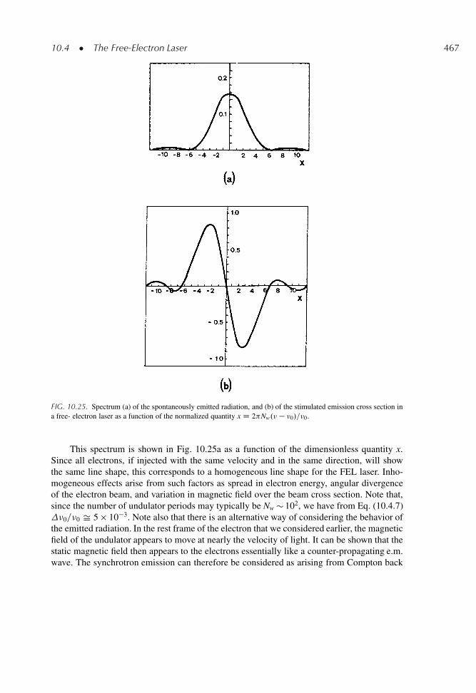
10.4 � The Free-Electron Laser 467
FIG. 10.25. Spectrum (a) of the spontaneously emitted radiation, and (b) of the stimulated emission cross section ina free- electron laser as a function of the normalized quantity x D 2 Nw.� � �0/=�0.
This spectrum is shown in Fig. 10.25a as a function of the dimensionless quantity x.Since all electrons, if injected with the same velocity and in the same direction, will showthe same line shape, this corresponds to a homogeneous line shape for the FEL laser. Inho-mogeneous effects arise from such factors as spread in electron energy, angular divergenceof the electron beam, and variation in magnetic field over the beam cross section. Note that,since the number of undulator periods may typically be Nw � 102, we have from Eq. (10.4.7)�0=�0 Š 5 � 10�3. Note also that there is an alternative way of considering the behavior ofthe emitted radiation. In the rest frame of the electron that we considered earlier, the magneticfield of the undulator appears to move at nearly the velocity of light. It can be shown that thestatic magnetic field then appears to the electrons essentially like a counter-propagating e.m.wave. The synchrotron emission can therefore be considered as arising from Compton back
468 10 � Gas, Chemical, Free Electron, and X-Ray Lasers
scattering of this “virtual” e.m. wave from the electron beam. For this reason the correspond-ing type of free electron laser (FEL) is sometimes referred to as operating in the Comptonregime (Compton FEL).
A calculation of the stimulated emission cross section requires a detailed analysis, whichwe do not consider here, of the interaction between a longitudinally propagating e.m. waveand the electron propagating in the wiggler magnetic field. We merely wish to point out that,unlike the situation that we have considered previously for all other lasers, the spectral dis-tribution of this cross section is not the same as that of the spontaneously emitted radiationbut is instead proportional to its frequency derivative. Accordingly, its shape will be as shownin Fig. 10.25b and one has gain on the low-frequency side and loss on the high-frequencyside of the transition. This unusual behavior is a result of the interaction being based upon alight-scattering process rather than absorption or emission from bound states.
So far, demonstrations of FEL operation have been made on several devices (more thanten) around the world, with oscillation wavelengths ranging from millimeter waves up tothe UV region. Many more FELs are now at various stages of planning. All of these lasersrequire large facilities since they involve using rather large e-beam accelerators. Historically,the first FEL was made to operate at � D 3.4�m using the Stanford University superconduct-ing linear accelerator..21/ Since the incoming e-beam consisted of 3.2-ps pulses separated by� D 84.7 ns, the cavity length L was chosen to be equal to the cavity round trip time (i.e.,L D c�=2 D 12.7 m) and the laser was operated in the synchronously mode-locked regime.One of the most important issues for a FEL is related to its efficiency. Since the emitted fre-quency depends on the electron energy [see Eq. (10.4.5)], the maximum energy that can beextracted from the electron is that which shifts its energy so that the corresponding operatingfrequency falls outside the gain curve. Consequently the maximum efficiency �max, defined asthe ratio between the maximum energy given to the laser beam and the initial electron energy,is approximately given by just �0=�0, i.e., is given by �max D .1=2Nw/. This means thatthe efficiency in such a device is rather limited .10�2–10�3/. Two ways of obtaining higherefficiency are being actively pursued: (1) The period of the magnet is gradually decreasedalong the e-beam direction so as to keep the �q=E2 ratio constant (tapered wiggler). (2) Theenergy remaining in the electron beam, after leaving the wiggler, is recovered by deceleratingthe electrons. Much higher efficiencies are predicted to be achievable using these approachesand indeed have been achieved to some degree. As a final comment we point out that theFELs described so far all use e-beam machines of high energy .E > 10 MeV/ and low cur-rent .I � 1–100 A/. Under these conditions, as previously discussed, the light emission canbe described as arising from Compton scattering of the virtual quanta of the magnetic fieldfrom individual electrons (Compton regime FEL). Free electron lasers using e-beams of lowerenergy .E D 1–2 MeV/ and much higher currents .I�10–20 kA/ have also been made tooperate. In this case, the electron-electron interaction becomes so strong that collective oscil-latory motions (plasma waves) are induced in the e-beam when interacting with the e.m. wavein the wiggler. The emission can then be looked upon as arising from scattering of the virtualquanta of the magnetic field from these collective motions rather than from single electrons.The emitted frequency, �0 D 2 =!0, is then no longer given by Eq. (10.4.5) but in fact down-shifted by the frequency of this collective motion. The phenomenon is analogous to Ramanscattering of light from molecular vibrations, and the corresponding laser is said to operate inthe FEL-Raman regime. Because of the lower value of electron energy involved, these lasersall oscillate in the millimeter wave region.
10.5 � X-ray Lasers 469
As a conclusion to this section we can say that the most attractive properties of FELs are:(1) Wide tunability; (2) excellent beam quality, close to the diffraction limit; and potentially,(3) very high efficiency, and thus very high laser power (the average power of the e-beam ofthe Stanford Linear Accelerator is about 200 kW). Free electron lasers are, however, inher-ently large and expensive machines, and interest in their applications is likely to be strongestin the frequency ranges where more conventional lasers are not so readily available e.g., inthe far IR (100–400�m) or in the vacuum ultraviolet .�<100 nm/.
10.5. X-RAY LASERS.22/
The achievement of coherent oscillation in the x-ray region has been a long soughtdream that is slowly but steadily coming true. The potential applications of x-ray lasersare indeed very important. They include in fact such possibilities as: (i) X-ray holographyor x-ray microscopy of e.g., living cells or cell constituents, allowing, respectively, three-dimensional or two-dimensional pictures with sub-nanometer resolution to be obtained. (ii)X-ray lithography, where patterns with extremely high resolution could be produced.
Before discussing what has been achieved so far in this wavelength region, let us indicatethe difficulties that have to be overcome to obtain x-ray laser operation. Starting with funda-mental considerations, we recall that the threshold pump power of a four-level laser is givenby Eq. (7.3.12) which is here reported for convenience
Pth D h�mp
�p
� A
� �(10.5.1)
The minimum threshold, Pmth, is of course attained for � D �.� D �0/ D �p, where �p
is the cross section at the peak of the transition. Furthermore, one must take into accountthat, in the x-ray region, the upper state lifetime � is established by the spontaneous life-time �sp. From Eqs. (2.4.29) and (2.3.15) one then gets 1=�p�sp / �2
0=gt.0/, independently ofthe transition matrix element j�j. For either Eq. (2.4.9b) (homogeneous line) or Eq. (2.4.28)(inhomogeneous line) one then finds that gt.0/ / 1=�0, where �0 indicates here the tran-sition linewidth for either a homogeneous or inhomogeneous line. Thus, in either case, fromEq. (10.5.1), with h�mp Š h�0, we obtain Pmth / �3
0�0. At frequencies in the VUV to softx-rays and at moderate pressures, we may assume that the linewidth is dominated by Dopplerbroadening. Hence, [see Eq. (2.5.18)],�0 / �0 and Pmth is expected to increase as �4
0 . At thehigher frequencies corresponding to the x-ray region, the linewidth is dominated by naturalbroadening since the radiative lifetime becomes very short (down to the femtosecond region).In this case one has �0 / 1=�sp / �3
0 and Pmth is expected to increase as �60 . Thus, if we
go from e.g., the green .� D 500 nm/ to the soft x-ray region .� Š 10 nm/ the wavelengthdecreases by a factor of 50 and Pmth increases by very many orders of magnitude. From amore practical viewpoint we note that multilayer dielectric mirrors for the x-ray region arelossy and difficult to make. A basic problem is that the difference in refractive index betweenvarious materials become very small in this region. Dielectric multi layers with a large num-ber of layers (hundreds) are therefore needed to achieve a reasonable reflectivity. Scatteringof light at the many interfaces then makes the mirrors very lossy and, furthermore, the mirrorshave difficulty to withstand the high intensity of a x-ray-laser beam. For these reasons, the

470 10 � Gas, Chemical, Free Electron, and X-Ray Lasers
x-ray lasers that have been operated so far, have operated without mirrors as ASE (amplifiedspontaneous emission) devices.
As a representative example, we will consider the soft x-ray laser based on 24-timesionized selenium .Se24C/ as the active medium,.23/ this being the first laser of a kind (the x-rayrecombination laser) which now includes a large number of materials. Pumping is achievedby the powerful second harmonic beam .� D 532 nm/ of the Novette laser (pulse energy�1 KJ, pulse duration �1 ns), consisting of one arm of the Nova laser, at Lawrence LivermoreLaboratory in the U.S.. The beam is focused to a fine line .d Š 200�m, l D 1.2 cm/ on a thinstripe (75 nm thick) of selenium evaporated on a 150-nm-thick foil of Formvar (Fig. 10.26).The foil could be irradiated from one or both sides. Exposed to the high intensity of thispump beam .�5 � 1013 W=cm2/, the foil explodes and a highly ionized selenium plasmais formed, whose shape is approximately cylindrical with a diameter d Š 200�m. Duringthe electron-ion recombination process, a particularly long-lived constituent of this plasma isformed, consisting of Se24C. This ion has the same ground-state electronic configuration asneutral Ne (1s22s22p6, see Fig. 10.1) and, accordingly, it is usually referred to as neon-likeselenium. Impact collisions with the hot plasma electrons .Te Š 1 keV/ then raises Se24Cfrom its ground state to excited states and population inversion between the states 2p53p and2p53s is achieved because the lifetime of the 3s ! ground state transition is much shorterthan the lifetime of the 3p ! 3s transition (both transitions are electric-dipole allowed). Witha pump configuration as in Fig. 10.26, a strong longitudinal emission due to ASE is observedon two lines (�1 D 20.63 nm and �2 D 20.96 nm) of the 2p53p ! 2p53s transition (seeFig. 10.1). Owing to the much higher nuclear charge of Se compared to Ne, these lines fallin the soft x-ray region. From the length dependence of the emitted energy it is deduced thata maximum single-pass gain, G D exp.�pNl/, of about 700 has been obtained. Note thatthis gain is still well below the “threshold” for ASE as defined in Sect. 2.9.2. In fact, for theexperimental situation described here, the emission solid angle is ˝ Š 10�4 sterad and thelinewidth is expected to be still dominated by Doppler broadening. From Eq. (2.9.4b) one thengets Gth Š 4.5 � 105. This means that the emitted intensity due to ASE is still much smallerthan the saturation intensity of the amplifier. Indeed, the x-ray output energy produced was anextremely small fraction .�10�10/ of the pump energy.
FIG. 10.26. Transverse irradiation geometry of a soft X-ray laser using the exploding-foil technique.
Problems 471
Since this first laser was demonstrated, research activity in this field has been verystrong..24/ Thus many new active media have been made to operate namely many more neon-like ions (from Ag37C to Ar8C), many hydrogen-like ions (from Al12C to C5C), lithium-likeions (from Si11C to Al10C) and nickel-like ions (from Au51 to Eu35C) ions. The range of theoscillation wavelength now extends from �3.6 to 47 nm while the single pass gain, G, gener-ally ranges from 10 to 103. To achieve the high pump powers required [see Eq. (10.5.1)] and, atthe same time, reduce the corresponding pump energy, picosecond or even femtosecond laserpulses are now also used for pumping. Amplified spontaneous emission (at � D 46.9 nm)has also been observed in neon-like Ar8C by passing a strong current pulse of short durationthrough a 1 � 10 cm long capillary filled with Ar.
10.6. CONCLUDING REMARKS
In this chapter, the most notable examples of lasers involving low-density media havebeen considered. In general these lasers tend to be more bulky, and often less efficient thanthe lasers considered in the previous chapter (notably semiconductor and diode-pumped solid-state lasers). For these reasons, whenever possible, these low-density lasers are tending to besuperseded by the solid-state-laser counterparts. This is for instance the case of the Argonlaser, which is facing a strong competition from the green beam emitted by a diode-pumpedNd laser (e.g., Nd:YVO4) with intracavity second-harmonic generation. This is also the case,at least for quite a few applications, of the red-emitting He-Ne laser, which is facing strongcompetition from red-emitting InGaAlP semiconductor lasers. Low-density lasers will how-ever survive in those frequency ranges which are not covered effectively by semiconductoror diode-pumped solid-state lasers. This is for instance the case for middle-infrared lasers,the CO2 lasers being the most notable example here, and for the lasers oscillating in the UV(e.g. excimer lasers) down to the X-ray spectral region. Another field of applications wherelow-density lasers will continue to perform well is where very high powers are required, withCO2 lasers, excimer lasers, and chemical lasers as important examples. Thus, as a conclusion,one can foresee that lasers based on low-density media will still maintain an important role inthe laser field.
PROBLEMS
10.1. List at least four lasers, using a low-density active medium, whose wavelengths fall in theinfrared.
10.2. List at least four lasers, using a low-density active medium, whose wavelengths fall in the UV tosoft-x-ray region. What are the problems to be faced in achieving laser action in the UV or x-rayregion?
10.3. For metalworking applications, a laser with cw output power >1 kW is required. Which lasersmeet this requirement?
472 10 � Gas, Chemical, Free Electron, and X-Ray Lasers
10.4. The 514.5 nm transition of an argon-ion laser is Doppler broadened to a line-width of �3.5 GHz.The cavity length of the laser is 100 cm and, when pumped three times above threshold, thelaser emits a power of 4 W in a TEM00 mode-profile. Assuming that the frequency of one ofthe oscillating TEM00 modes coincides with the center of the gain line, calculate the number ofTEM00 modes which are expected to oscillate.
10.5. Consider the argon-ion laser described in the previous problem and assume that the laser ismode-locked by an acousto-optic modulator. Calculate: (i) The duration and the peak power ofthe mode-locked pulses. (ii) The drive frequency of the rf oscillator.
10.6. Assume that the bond between the two nitrogen atoms of the N2 molecule can be simulated by aspring of suitable elastic constant. Knowing the vibrational frequency (Fig. 10.9) and the atomicmass calculate the elastic constant. Compare this constant with that obtainable from the groundstate curve of Fig. 10.19.
10.7. Show that, if the elastic constant of the N-N bond is taken to be the same as that of the iso-electronic CO molecule, the .� 0 D 1/ ! .� D 0/ transition wavelength of the N2 molecule isapproximately the same as that of the CO molecule.
10.8. Assume that each of the two oxygen-carbon bonds of the CO2 molecule can be simulated by aspring with elastic constant k. With the assumption that there is no interaction between the twooxygen atoms and knowing the �1 frequency .�1 D 1337 cm�1/, calculate this constant.
10.9. Knowing the elastic constant k between the two oxygen-carbon bonds, obtained in the previousproblem, calculate the expected frequency �3 of the asymmetric stretching mode and comparethe result with the value shown in Fig. 10.9.
10.10. Show that each C-O bond of the CO2 molecule cannot be simulated by elastic springs if theharmonic oscillation corresponding to the bending mode of frequency �2 has to be calculated.
10.11. From the knowledge that, for a Boltzmann distribution, the maximum population of the upperlaser level of a CO2 molecule occurs for the rotational quantum number J0 D 21 (see Fig. 10.11),calculate the rotational constant B [assume T D 400 K, which corresponds to an energy kT suchthat .kT=h/ Š 280 cm�1]. From this value then calculate the equilibrium distance between theC atom and each O atom.
10.12. Using the result of the previous problem, calculate the frequency spacing (in cm�1) between therotational lines of the CO2 laser transition [assume that the rotational line constant of the lowerlaser level is the same as that of the upper laser level, and remember that only levels with oddvalues of J are occupied in a CO2 molecule].
10.13. The linewidth, due to collision broadening, of the CO2 laser transition is given by �c D7.58 . CO2 C 0.73 N2 C 0.6 He/p.300=T/1=2 MHz, where the are the fractional partialpressures of the gas mixture, T is the gas temperature and p is the total pressure (in torr) (seeexample 3.3). Taking a ratio of the partial pressures of CO2, N2, and He molecules of 1:1:8 andassuming a separation between rotational lines of the CO2 laser transition of�r Š 2cm�1, cal-culate the total gas pressure needed to make all the rotational lines merge together. What wouldthe width of the gain curve be?
10.14. Consider a CO2 laser with high enough pressure to have all its rotational lines merged together.If this laser were mode-locked, what would be the order of magnitude of the corresponding laserpulse-width?
10.15. Show that a reaction energy of 31.6 kcal/mole, as in the HF cold reaction [see Eq. (10.3.1)], isequivalent to an energy of 1.372 eV released for each molecular reaction.
References 473
10.16. Consider the cold reaction of Fig. 10.22a and take the values shown in the figure for the relativepopulations of HF molecules which, after reaction, are left in the first three vibrational levels.Calculate the fraction, �, of heat released in the reaction which goes into vibrational energy.
10.17. Repeat the previous calculation for the hot reaction of Fig. 10.22b.
10.18. To reach the final end products of the cold reaction, see Eq. (10.3.1), one can choose a reactionpath-way where one first dissociates the H2 molecule, to obtain the single atoms F, H, and H, andthen let the fluorine and one hydrogen atom recombine together. Similarly, for the hot reaction,see Eq. (10.3.2), one can first dissociate molecular fluorine and then recombine one fluorinewith the hydrogen atom. Given the two possibilities, relate the difference in heat of reaction ofthese two reactions to the difference in dissociation energy between the fluorine and hydrogenmolecules.
References
1. R. Arrathoon, Helium-Neon Lasers and the Positive Column, in Lasers, ed. by A. K. Levine and A. J. De Maria(Marcel Dekker, New York, 1976), Vol. 4, Chap. 3.
2. W. B. Bridges, Atomic and Ionic Gas Lasers, in Methods of Experimental Physics, ed. by C. L. Tang (Academic,New York, 1979), Vol. 15, pp. 33–151.
3. A. Javan, W. R. Bennett, and D. H. Herriott, Population Inversion and Continuous Optical Maser Oscillation ina Gas Discharge Containing a He-Ne Mixture, Phys. Rev. Lett., 6, 106 (1961).
4. C. E. Webb, Metal Vapor Lasers: Recent Advances and Applications, in Gas Flow and Chemical Lasers, SpringerProceedings in Physics N. 15, ed. by S. Rosenwork (Springer-Verlag, Berlin, 1987), pp. 481–494.
5. C. C. Davis and T. A. King, Gaseous Ion Lasers, in Advances in Quantum Electronics, ed. by D. W. Goodwin(Academic, New York, 1975), Vol. 3, pp. 170–437.
6. D. H. Dunn and J. N. Ross, The Argon Ion Laser, in Progress in Quantum Electronics, ed. by J. H. Sanders andS. Stenholm (Pergamon, London, 1977), Vol. 4, pp. 233–270.
7. W. B. Bridges, Laser Oscillation in Singly Ionized Argon in the Visible Spectrum, Appl. Phys. Letters 4,128 (1964).
8. P. K. Cheo, CO2 Lasers, in Lasers, ed. by A. K. Levine and A. J. De Maria (Marcel Dekker, New York, 1971),Vol. 3, Chap. 2.
9. A. J. De Maria, Review of High-Power CO2 Lasers, in Principles of Laser Plasmas, ed. by G. Bekefi (Wiley-Interscience, New York, 1976), Chap. 8.
10. C. K. N. Patel, W. L. Faust, and R. A. Mc Farlane, CW Laser Action on Rotational Transitions of the˙Cu ! ˙C
gVibrational Band of CO2, Bull. Am. Phys. Soc. 9, 500 (1964).
11. D. R. Hall and C. A. Hill, Radiofrequency-Discharge-Excited CO2 Lasers, in Handbook of Molecular Lasers ed.by P. Cheo (Marcel Dekker, New York, 1987) Chapt. 3.
12. K. M. Abramski, A. D. Colley, H. J. Baker, and D. R. Hall, Power Scaling of Large-Area TransverseRadiofrequency Discharge CO2 Lasers, Appl. Phys. Letters, 54, 1833–1835 (1989).
13. P. E. Jackson, H. J. Baker, and D. R. Hall, CO2 Large-Area Discharge Laser Using an Unstable-WaveguideHybrid Resonator, Appl. Phys. Letters, 54, 1950–1952 (1989).
14. R. E. Center, High-Power, Efficient Electrically-Excited CO Laser, in Laser Handbook, ed. by M. L. Stitch(North-Holland, Amsterdam, 1979), Vol. 3, pp. 89–133.
15. C. S. Willet, An Introduction to Gas Lasers: Population Inversion Mechanisms (Pergamon-Press, Oxford, 1974),Secs. 6.2.1 and 6.2.3.
16. N. G. Basov, V. A. Danilychev, and Yu. M. Popov, Stimulated Emission in the Vacuum Ultraviolet Region, SovietJ. Quantum Electron., 1, 18 (1971).
17. J. J. Ewing, Excimer Lasers, in Laser Handbook, ed. by M. L. Stitch (North-Holland, Amsterdam, 1979), Vol. 3,pp. 135–197.

474 10 � Gas, Chemical, Free Electron, and X-Ray Lasers
18. A. N. Chester, Chemical Lasers, in High-Power Gas Lasers, ed. by E. R. Pike (The Institute of Physics, Bristoland London, 1975), pp. 162–221.
19. C. J. Ultee, Chemical and Gas-Dynamic Lasers, in Laser Handbook, ed. by M. L. Stitch and M. Bass (North-Holland, Amsterdam, 1985), Vol. 3, pp. 199–287.
20. G. Dattoli and R. Renieri, Experimental and Theoretical Aspects of the Free-Electron Lasers, in Laser Handbook,ed. by M. L. Stitch (North-Holland, Amsterdam, 1979), Vol. 4, pp. 1–142.
21. D. A. G. Deacon, L. R. Elias, J. M. J. Madey, G. J. Ramian, H. A. Schwettman, and T. I. Smith, First Operationof a Free-Electron Laser, Phys. Rev. Lett. 38, 892 (1977).
22. R. C. Elton, X-Ray Lasers (Acedemic, Boston 1990).23. D. L. Matthews et. al., Demonstration of a Soft X-ray Amplifier, Phys. Rev Lett. 54, 110 (1985).24. X-Ray Lasers 1996, ed. by S. Svanberg and C. G. Wahlstrom, Institute of Physics Conference Series N. 151
(Institute of Physics, Bristol 1996).
11
Properties of Laser Beams
11.1. INTRODUCTION
In Chap. 1 it was stated that the most characteristic properties of laser beams are(1) monochromaticity, (2) coherence (spatial and temporal), (3) directionality, (4) brightness.The material presented in earlier chapters allows us to now examine these properties in moredetail and compare them with the properties of conventional light sources (thermal sources).
In most cases of interest to us, the spectral bandwidth of the light source ! is muchsmaller than the mean frequency <!> of the spectrum (quasi-monochromatic wave). In thiscase, the electric field of the wave, at position r and time t, can be written as
E.r, t/ D A.r, t/ exp j Œ<!>t � �.r, t/� (11.1.1)
where A.r, t/ and �.r, t/ are both slowly varying over an optical period, i.e.,
�ˇˇ @A
A@ t
ˇˇ ,
ˇˇ@ �@ t
ˇˇ� � h!i (11.1.2)
We then define the intensity of the beam as
I.r, t/ D E.r, t/E�.r, t/ D jA.r, t/j2 (11.1.3)
11.2. MONOCHROMATICITY
We have seen in Sects. 7.9–7.11 that the frequency fluctuations of a c.w. single-modelaser mostly arise from phase fluctuations rather than amplitude fluctuations. Amplitudefluctuations come in fact from pump or cavity loss fluctuations. They are usually very
O. Svelto, Principles of Lasers,c
475DOI: 10.1007/978-1-4419-1302-9 11, � Springer Science+Business Media LLC 2010
476 11 � Properties of Laser Beams
small .�1%/ and can be further reduced by suitable electronically-controlled feedbackloops. To first order we can thus take A.t/ to be constant for a single-mode laser andso consider its degree of monochromaticity to be determined by frequency fluctuations.The theoretical limit to this monochromaticity arises from zero-point fluctuations and isexpressed by Eq. (7.9.2). However, this limit generally corresponds to a very low valuefor the oscillating bandwidth, �L, which is seldom reached in practice. In the exam-ple 7.9, for instance, the value of �L is calculated to be �0.4 mHz for a He-Ne laserwith 1 mW output power. A notable exception to this situation occurs for a semiconduc-tor laser, where, due to the short length and high loss of the laser cavity, this limit isvery much higher .�L Š 1 MHz/ and the actual laser linewidth is indeed often deter-mined by these quantum fluctuations. Otherwise, in most other cases, technical effectssuch as vibrations and thermal expansion of the cavity are dominant in determining thelaser linewidth �L. If a monolithic structure is used for the laser cavity configuration,as in the non-planar ring oscillator of Fig. 7.26, typical values of �L may fall in the10�50 kHz range. Much smaller linewidths (down to �0.1 Hz) can be obtained by stabiliz-ing the laser frequency against an external reference, as discussed in Sect. 7.10. In pulsedoperation the minimum linewidth is obviously limited by the inverse of the pulse dura-tion �p. For example, for a single-mode Q-switched laser, assuming �p Š 10 ns, one has�L Š 100 MHz.
In the case of a laser oscillating on many modes, the monochromaticity is obviouslyrelated to the number of oscillating modes. We recall, for example, that in mode-locked oper-ation, pulses down to a few tens of femtoseconds have been obtained. In this case, actually,the corresponding laser bandwidth is in the range of a few tens of THz and the condition forquasi-monochromatic radiation no longer holds well.
The degree of monochromaticity required depends, of course, on the given application.Actually, the very narrowest laser linewidths are only needed for the most sophisticatedapplications dealing with metrology and with fundamental measurements in physics (e.g.gravitational wave detection). For other more common applications, such as interferomet-ric measurements of distances, coherent laser radar, and coherent optical communications,the required monochromaticity falls in the 10–100 kHz range while a monochromaticity of�1 MHz is typical of what is needed for much of high resolution spectroscopy and it is cer-tainly enough for optical communications using wavelength-division-multiplexing (WDM).For some applications, of course, laser monochromaticity is not relevant. This is certainly thecase for important applications such as laser material working and for most applications inthe biomedical field.
11.3. FIRST-ORDER COHERENCE.1/
In Chap. 1 the concept of coherence of an e.m. wave was introduced in an intuitivefashion, with two types of coherence being distinguished: (1) spatial and (2) temporal coher-ence. In this section we give a more detailed discussion of these two concepts. In fact, as willbe better appreciated by the end of this chapter, it turns out that spatial and temporal coherencedescribe the coherence properties of an e.m. wave only to first order.
11.3 � First-Order Coherence 477
11.3.1. Degree of Spatial and Temporal Coherence
In order to describe the coherence properties of a light source, we can introduce a wholeclass of correlation functions for the corresponding field. For the moment, however, we willlimit ourselves to looking at the first-order functions.
Suppose that a measurement of the field is performed at some point r1 in a time intervalbetween 0 and T. We can then obtain the product E.r1, t1/E�.r1, t2/ where t1 and t2 are giventime instants within the time interval 0�T. If the measurement is now repeated a large numberof times, we can calculate the average of the above product over all the measurements. Thisaverage is called the ensemble average and written as
� .1/.r1, r1, t1, t2/ D hE.r1, t1/E�.r1, t2/i (11.3.1)
For the remainder of this section as well as in the next two sections, we will consider the caseof a stationary beam,� as would for instance apply to a single-mode c.w. laser or to a c.w.laser oscillating on many modes that are not locked in phase, or to a c.w. thermal light source.In these cases, by definition, the ensemble average will only depend upon the time difference� D t1–t2 and not upon the particular times t1 and t2. We can then write
� .1/.r1, r1, t1, t2/ D � .1/.r1, r1, �/ D hE.r1, t C �/E�.r1, t/i (11.3.2)
where we have set t D t2 and � .1/ only depends upon � . If now the field, besides beingstationary is also ergodic (a condition that also usually applies to the cases considered above),then, by definition, the ensemble average is the same as the time average. We can then write
� .1/.r1, r1, �/ D limT!1
1
T
TZ0
E.r1, t C �/ E�.r1, t/dt (11.3.3)
Note that, the definition of � .1/ in terms of a time average is perhaps easier to deal with thanthat based on ensemble averages. However, the definition of � .1/ in terms of an ensembleaverage is more general and, in the form given by Eq. (11.3.1), can be applied also to nonstationary beams, as we shall see in Sect. 11.3.4.
Having defined the first-order correlation function � .1/ at a given point r1, we can definea normalized function � .1/.r1, r1, �/ as follows
� .1/ D hE.r1, t C �/ E�.r1, t/ihE.r1, t/ E�.r1, t/i1=2hE.r1, t C �/ E�.r1, t C �/i1=2
(11.3.4)
Note that, for a stationary beam, the two ensemble averages in the denominator of Eq. (11.3.4)are equal to each other and, according to Eq. (11.1.3), are both equal to the average beamintensity hI.r1, t/i. The function � .1/, as defined by Eq. (11.3.4), is referred to as the complexdegree of temporal coherence while its magnitude,
ˇ� .1/
ˇ, as the degree of temporal coherence.
Indeed � .1/ gives the degree of correlation between the fields at the same point r1 at two
� A process is said to be stationary when the ensemble average of any variable that describes it (e.g., the analyticsignal or the beam intensity, in our case), is independent of time.
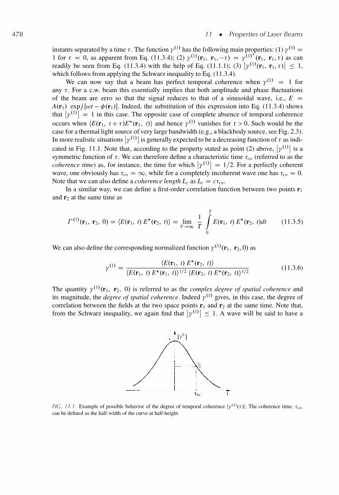
478 11 � Properties of Laser Beams
instants separated by a time � . The function � .1/ has the following main properties: (1) � .1/ D1 for � D 0, as apparent from Eq. (11.3.4); (2) � .1/.r1, r1, ��/ D � .1/�
.r1, r1, �/ as canreadily be seen from Eq. (11.3.4) with the help of Eq. (11.1.1); (3)
ˇ� .1/.r1, r1, �/
ˇ 1,which follows from applying the Schwarz inequality to Eq. (11.3.4).
We can now say that a beam has perfect temporal coherence when � .1/ D 1 forany � . For a c.w. beam this essentially implies that both amplitude and phase fluctuationsof the beam are zero so that the signal reduces to that of a sinusoidal wave, i.e., E DA.r1/ exp j Œ!t � �.r1/�. Indeed, the substitution of this expression into Eq. (11.3.4) showsthat
ˇ� .1/
ˇ D 1 in this case. The opposite case of complete absence of temporal coherenceoccurs when hE.r1, t C �/E�.r1, t/i and hence � .1/ vanishes for � > 0. Such would be thecase for a thermal light source of very large bandwidth (e.g., a blackbody source, see Fig. 2.3).In more realistic situations
ˇ� .1/
ˇis generally expected to be a decreasing function of � as indi-
cated in Fig. 11.1. Note that, according to the property stated as point (2) above,ˇ� .1/
ˇis a
symmetric function of � . We can therefore define a characteristic time �co (referred to as thecoherence time) as, for instance, the time for which
ˇ� .1/
ˇ D 1=2. For a perfectly coherentwave, one obviously has �co D 1, while for a completely incoherent wave one has �co D 0.Note that we can also define a coherence length Lc as Lc D c�co.
In a similar way, we can define a first-order correlation function between two points r1
and r2 at the same time as
� .1/.r1, r2, 0/ D hE.r1, t/ E�.r2, t/i D limT!1
1
T
TZ0
E.r1, t/ E�.r2, t/dt (11.3.5)
We can also define the corresponding normalized function � .1/.r1, r2, 0/ as
� .1/ D hE.r1, t/ E�.r2, t/ihE.r1, t/ E�.r1, t/i1=2 hE.r2, t/ E�.r2, t/i1=2
(11.3.6)
The quantity � .1/.r1, r2, 0/ is referred to as the complex degree of spatial coherence andits magnitude, the degree of spatial coherence. Indeed � .1/ gives, in this case, the degree ofcorrelation between the fields at the two space points r1 and r2 at the same time. Note that,from the Schwarz inequality, we again find that
ˇ� .1/
ˇ 1. A wave will be said to have a
FIG. 11.1. Example of possible behavior of the degree of temporal coherence j�.1/.�/j. The coherence time, �co,can be defined as the half-width of the curve at half-height.
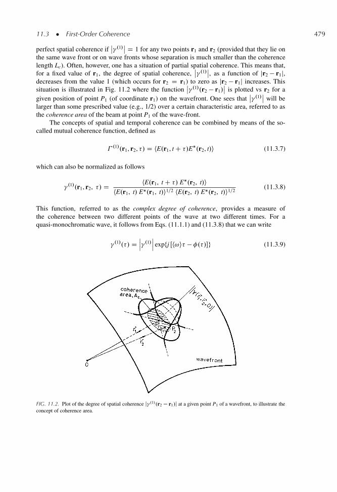
11.3 � First-Order Coherence 479
perfect spatial coherence ifˇ� .1/
ˇ D 1 for any two points r1 and r2 (provided that they lie onthe same wave front or on wave fronts whose separation is much smaller than the coherencelength Lc). Often, however, one has a situation of partial spatial coherence. This means that,for a fixed value of r1, the degree of spatial coherence,
ˇ� .1/
ˇ, as a function of jr2 � r1j,
decreases from the value 1 (which occurs for r2 D r1) to zero as jr2 � r1j increases. Thissituation is illustrated in Fig. 11.2 where the function
ˇ� .1/.r2 � r1/
ˇis plotted vs r2 for a
given position of point P1 (of coordinate r1) on the wavefront. One sees thatˇ� .1/
ˇwill be
larger than some prescribed value (e.g., 1/2) over a certain characteristic area, referred to asthe coherence area of the beam at point P1 of the wave-front.
The concepts of spatial and temporal coherence can be combined by means of the so-called mutual coherence function, defined as
� .1/.r1, r2, �/ D hE.r1, t C �/E�.r2, t/i (11.3.7)
which can also be normalized as follows
� .1/.r1, r2, �/ D hE.r1, t C �/ E�.r2, t/ihE.r1, t/ E�.r1, t/i1=2 hE.r2, t/ E�.r2, t/i1=2
(11.3.8)
This function, referred to as the complex degree of coherence, provides a measure ofthe coherence between two different points of the wave at two different times. For aquasi-monochromatic wave, it follows from Eqs. (11.1.1) and (11.3.8) that we can write
� .1/.�/ Dˇ� .1/
ˇexpfj Œh!i� � �.�/�g (11.3.9)
FIG. 11.2. Plot of the degree of spatial coherence j�.1/.r2 � r1/j at a given point P1 of a wavefront, to illustrate theconcept of coherence area.
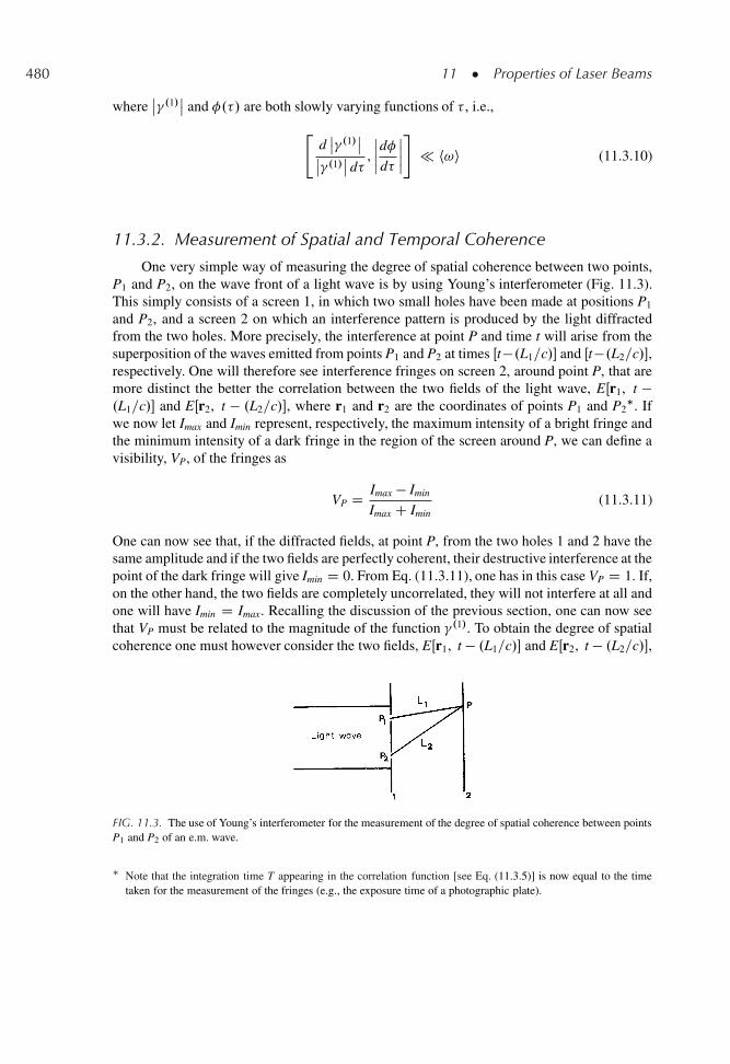
480 11 � Properties of Laser Beams
whereˇ� .1/
ˇand �.�/ are both slowly varying functions of � , i.e.,
"dˇ� .1/
ˇˇ� .1/
ˇd�
,
ˇˇd�d�
ˇˇ#
� h!i (11.3.10)
11.3.2. Measurement of Spatial and Temporal Coherence
One very simple way of measuring the degree of spatial coherence between two points,P1 and P2, on the wave front of a light wave is by using Young’s interferometer (Fig. 11.3).This simply consists of a screen 1, in which two small holes have been made at positions P1
and P2, and a screen 2 on which an interference pattern is produced by the light diffractedfrom the two holes. More precisely, the interference at point P and time t will arise from thesuperposition of the waves emitted from points P1 and P2 at times Œt�.L1=c/� and Œt�.L2=c/�,respectively. One will therefore see interference fringes on screen 2, around point P, that aremore distinct the better the correlation between the two fields of the light wave, EŒr1, t �.L1=c/� and EŒr2, t � .L2=c/�, where r1 and r2 are the coordinates of points P1 and P2
�. Ifwe now let Imax and Imin represent, respectively, the maximum intensity of a bright fringe andthe minimum intensity of a dark fringe in the region of the screen around P, we can define avisibility, VP, of the fringes as
VP D Imax � Imin
Imax C Imin(11.3.11)
One can now see that, if the diffracted fields, at point P, from the two holes 1 and 2 have thesame amplitude and if the two fields are perfectly coherent, their destructive interference at thepoint of the dark fringe will give Imin D 0. From Eq. (11.3.11), one has in this case VP D 1. If,on the other hand, the two fields are completely uncorrelated, they will not interfere at all andone will have Imin D Imax. Recalling the discussion of the previous section, one can now seethat VP must be related to the magnitude of the function � .1/. To obtain the degree of spatialcoherence one must however consider the two fields, EŒr1, t � .L1=c/� and EŒr2, t � .L2=c/�,
FIG. 11.3. The use of Young’s interferometer for the measurement of the degree of spatial coherence between pointsP1 and P2 of an e.m. wave.
� Note that the integration time T appearing in the correlation function [see Eq. (11.3.5)] is now equal to the timetaken for the measurement of the fringes (e.g., the exposure time of a photographic plate).
11.3 � First-Order Coherence 481
at the same time. This then requires that the point P be chosen so that L1 D L2. In this case, itwill be shown in example 11.1 that
VP D j� .1/.r1, r2, 0/j (11.3.12)
On the other hand, if the two holes 1 and 2 do not produce the same amplitudes, i.e., the sameillumination, at point P, instead of Eq. (11.3.12) one has
VP D 2ŒhI1i hI2i�1=2
hI1i C hI2iˇˇ� .1/.r1, r2, 0/
ˇˇ (11.3.13)
where hI1i and hI2i are the average intensities of the ligth diffracted to point P from the twoholes. Note also that, for the general point P shown in Fig. 11.3, the visibility VP can be shownto be equal to
ˇ� .1/.r1, r2, �/
ˇ, where � D .L2 � L1/=c.
Example 11.1. Calculation of the fringe visibility in Young’s interferometer. The field E.rP, t0/, at pointP of Fig. 11.3 and time t0, can be expressed as a superposition of the fields diffracted from holes 1 and 2at times .t0 � L1=c/ and .t0 � L2=c/, respectively. We can then write
E.rP, t0/ D K1 E.r1, t0 � L1=c/C K2 E.r2, t0 � L2=c/ (11.3.14)
where E.r1, t0 � L1=c/ and E.r2, t0 � L2=c/ are the fields at points P1 and P2 while K1 and K2 representthe fractions of these two fields which are diffracted to position P, respectively. The factors K1 and K2
are expected to be inversely proportional to L1 and L2 and to also depend on the hole dimensions and theangle between the incident wave and the wave diffracted from P1 and P2. Since the diffracted secondarywavelets are always a quarter of a period out of phase with the incident wave [see also the discussion of“Huygens wavelets” appearing in Sect. 4.6] it follows that
K1 D jK1j exp Œ�.j =2/� (11.3.15a)
K2 D jK2j exp Œ�.j =2/� (11.3.15b)
If we now define t1 D t0 � L2=c and � D .L2=c/� .L1=c/, Eq. (11.3.14) can be written as
E D K1 E.r1, t C �/C K2 E.r2, t/ (11.3.16)
According to Eq. (11.1.3), the intensity at the point P can be written as I D EE� D jK1 E.r1, t C �/ CK2 E.r2, t/j2, where Eq. (11.3.16) has been used. From this expression, with the help of Eq. (11.3.15),one obtains
I D I1.t C �/C I2.t/C 2Re ŒK1 K�2 E.r1, t C �/E� .r2, t/� (11.3.17)
where Re stands for real part. In the previous expressions, I1 and I2 are the intensities, at point P, due tothe emission from point P1 alone and point P2 alone, respectively, and are given by
I1 D jK1j2jE.r1, t C �/j2 D jK1j2 I.r1, t C �/ (11.3.18a)
I2 D jK2j2jE.r2, t/j2 D jK2j2 I.r2, t/ (11.3.18b)
482 11 � Properties of Laser Beams
where I.r1, t C �/ and I.r2, t/ are the intensities at points P1 and P2. Taking the time average of bothsides of Eq. (11.3.17) and using Eq. (11.3.7), we find
hIi D hI1i C hI2i C 2jK1jjK2jReŒ� .1/.r1, r2, �/� (11.3.19)
where equations (11.3.15) have also been used. Equation (11.3.19) can be expressed in terms of � .1/ bynoting that from Eq. (11.3.8) we have
� .1/ D � .1/ŒhI.r1, t C �/ihI.r2, t/i�1=2 (11.3.20)
The substitution of Eq. (11.3.20) in Eq. (11.3.19) with the help of Eq. (11.3.18) giveshIi D hI1i C hI2i C 2.hI1ihI2i/1=2 ReŒ� .1/.r1, r2, �/�. From Eq. (11.3.9) we then get
hIi D hI1i C hI2i C 2.hI1ihI2i/1=2j� .1/j cosŒh!i� � �.�/� (11.3.21)
Now, since both j� .1/j and �.�/ are slowly varying as a function of � , it follows that the variation ofintensity hIi as P is changed, i.e., the fringe pattern, is due to the rapid variation of the cosine term withits argument h!i� . So, in the region around P, we have
Imax D hI1i C hI2i C 2.hI1ihI2i/1=2j� .1/j (11.3.22a)
Imin D hI1i C hI2i � 2.hI1ihI2i/1=2j� .1/j (11.3.22b)
and therefore, from equation (11.3.11)
VP D 2 .hI1ihI2i/1=2
hI1i C hI2iˇˇ� .1/.r1, r2, �/
ˇˇ (11.3.23)
For the case � D .L2=c/� .L1=c/ D 0, Eq. (11.3.23) reduces to Eq. (11.3.13).
The measurement of the degree of temporal coherence is usually performed by means ofthe Michelson interferometer (Fig. 11.4a). Let P be the point where the temporal coherenceof the wave is to be measured. A combination of a suitably small diaphragm placed at P anda lens with its focus at P transforms the incident wave into a plane wave (see Fig. 11.12).This wave then falls on a partially reflecting mirror S1 (of reflectivity R D 50%) which splitsthe beam into the two beams A and B. These beams are reflected back by mirrors S2 and S3
(both of reflectivity R D 100%) and recombine to form the beam C. Since the waves A andB interfere, the illumination in the direction of C will be either light or dark according towhether 2.L3 � L2/ is an even or odd number of half wavelengths. Obviously this interferencewill only be observed as long as the difference L3 � L2 does not become so large that thetwo beams A and B become uncorrelated in phase. Thus, for a partially coherent wave, theintensity Ic of beam C as a function of 2.L3 � L2/ will behave as shown in Fig. 11.4b. At agiven value of the L3 � L2 difference between the lengths of the interferometer arms, i.e., ata given value of the delay � D 2.L3 � L2/=c between the two reflected waves, one can again
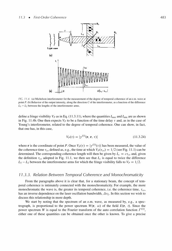
11.3 � First-Order Coherence 483
FIG. 11.4. (a) Michelson interferometer for the measurement of the degree of temporal coherence of an e.m. wave atpoint P. (b) Behavior of the output intensity, along the direction C of the interferometer, as a function of the differenceL3 � L2 between the lengths of the interferometer arms.
define a fringe visibility VP as in Eq. (11.3.11), where the quantities Imax and Imin are as shownin Fig. 11.4b. One then expects VP to be a function of the time delay � and, as in the case ofYoung’s interferometer, related to the degree of temporal coherence. One can show, in fact,that one has, in this case,
VP.�/ D j� .1/.r, r, �/j (11.3.24)
where r is the coordinate of point P. Once VP.�/ D j� .1/.�/j has been measured, the value ofthe coherence time �co defined as, e.g., the time at which VP.�co/ D 1=2 (see Fig. 11.1) can bedetermined. The corresponding coherence length will then be given by Lc D c�co and, giventhe definition �co adopted in Fig. 11.1, we then see that Lc is equal to twice the differenceL3 � L2 between the interferometer arms for which the fringe visibility falls to VP D 1=2.
11.3.3. Relation Between Temporal Coherence and Monochromaticity
From the paragraphs above it is clear that, for a stationary beam, the concept of tem-poral coherence is intimately connected with the monochromaticity. For example, the moremonochromatic the wave is, the greater its temporal coherence, i.e. the coherence time, �co,has an inverse dependence on the laser oscillation bandwidth,�L. In this section we wish todiscuss this relationship in more depth.
We start by noting that the spectrum of an e.m. wave, as measured by, e.g., a spec-trograph, is proportional to the power spectrum W.r, !/ of the field E.r, t/. Since thepower spectrum W is equal to the Fourier transform of the auto correlation function � .1/,either one of these quantities can be obtained once the other is known. To give a precise
484 11 � Properties of Laser Beams
Example 11.2. Coherence time and bandwidth for a sinu-soidal wave with random phase jumps. We will assumethat the time behavior of the field at a given point isdescribed by a sinusoidal wave with constant amplitudeand with phase undergoing random jumps (see Fig. 2.9).The correlation function � .1/.�/ for this wave has beencalculated in Appendix B to be � .1/.�/ / exp �.j� j=�c/
where �c is the average time between two consecutivephase jumps. According to Eq. (11.3.26) one then gets
�2� D
1R0�2 expŒ�.2�=�c/�d�
1R0
expŒ�.2�=�c/�d�D �2
c
4
1R0
x2 expŒ�x�dx
1R0
expŒ�x�dxD �2
c
2
where x D 2�=�c. We thus get �� D �c=p
2. The powerspectrum, W.� � �0/, of this signal is then described bya Lorentzian function (see again Appendix B) so that,according to Eq. (11.3.27) we can write
�2� D
1R0.� � �0/
2h
11C4�2.���0/2�2
c
i 2d.� � �0/
1R0
h1
1C4�2.���0/2�2c
i 2d.� � �0/
D
D 1
4 2�2c
1R0
x2h
11Cx2
i 2dx
1R0
h1
1Cx2
i 2dx
where x D 2 .� � �0/�c. It turns out that the two inte-grals on the right-hand side of the above equation areboth equal to . =4/.11/ so that �� D .1=2 �c/. Fromthe previous calculations one then finds that the product���� is equal to 1=.2
p2/ , i.e., it is
p2 times larger
than the minimum value, 1=4 , that holds for a Gaussianspectrum.
expression for the relation between �co and�L we need to redefine these two quantitiesin an appropriate way. So we will define �co
as the variance, �� , of the function j� .1/.�/j2,i.e., such that
.�� /2 D
�Z C1
�1.� � h�i/2j� .1/.�/j2d�
�.�Z C1
�1j� .1/.�/j2d�
�,
where the mean value h�i is defined byh�i D Œ
R� j� .1/.�/j2d��=Œ
R j� .1/.�/j2d��.As a short-hand notation for the aboveexpression, we will write
.�� /2 D hŒ� � h�i�2i (11.3.25)
Since j� .1/.��/j2 D j� .1/.�/j2, one hash�i D 0 and Eq. (11.3.25) reduces to
.�� /2 D h�2i (11.3.26)
The coherence time defined in this wayis conceptually simpler, although sometimesinvolving lengthier calculation, than thatdefined earlier, i.e., the half-width at half-height of the curve j� .1/.�/j2, see Fig. 11.1.In fact, if j� .1/.�/j2 were an oscillatory func-tion of the coherence time, �co, as definedin Fig. 11.1, would not be uniquely deter-mined. Similarly we define the laser oscilla-tion bandwidth�L as the variance of W2.�/,i.e., such that
.�L/2 D .��/
2 D hŒ� � h�i�2i (11.3.27)
where h�i, the mean frequency of the spec-trum, is given by h�i D Œ
R�W2d��
ıŒR
W2d��. Now, since W and � .1/ are relatedby a Fourier transform, it can be shown that�� and �� , as we have just defined them,
satisfy the condition
�� �� .1=4 / (11.3.28)
The relation (11.3.28) is closely analogous to the Heisenberg uncertainty relation and can beproved using the same procedure as used to derive the uncertainty relation..2/ The equality signin Eq. (11.3.28) applies when j�.1/.�/j [and hence W.�/] are Gaussian functions. This case isobviously the analogue of the minimum uncertainty wave packets of quantum mechanics..2/
11.3 � First-Order Coherence 485
11.3.4. Nonstationary Beams�
We will now briefly consider the case of a nonstationary beam. In this case, by definition,the function � .1/ in Eq. (11.3.1) depends on both t1 and t2 and not only on their difference� D t1 � t2. Examples would include an amplitude-modulated laser, an amplitude-modulatedthermal light source, a Q-switched or a mode-locked laser. For a nonstationary beam, thecorrelation function can be obtained as the ensemble average of many measurements of thefield in a time interval between 0 and T, where the origin of the time interval is synchronizedto the driving signal (e.g., synchronized to the amplitude modulator for a mode-locked laseror the Pockels cell driver for a Q-switched laser). The degree of temporal coherence at a givenpoint r can then be defined as
� .1/.t1, t2/ D hE.t1/ E�.t2/ihE.t1/ E�.t1/i1=2 hE.t2/ E�.t2/i1=2
(11.3.29)
where t1 and t2 are two given times, in the interval 0-T, and where all signals are measured atpoint r. We can now say that the beam has a perfect temporal coherence if j� .1/.t1, t2/j D 1for all times t1 and t2. According to this definition we can see that a nonstationary beamwithout amplitude and phase fluctuations has a perfect temporal coherence. In the absenceof fluctuations, in fact, the products E.t1/E�.t2/, E.t1/E�.t1/, and E.t2/E�.t2/ appearing inEq. (11.3.29) remain the same for all measurements of the ensemble. These products are thusequal to the corresponding ensemble averages and � .1/.t1, t2/ reduces to
� .1/.t1, t2/ D E.t1/E�.t2/jE.t1/jjE.t2/j (11.3.30)
From Eq. (11.3.30) we then immediately see that j� .1/j D 1. According to this definition oftemporal coherence, the coherence time of a nonstationary beam, e.g., of a mode-locked laser,is infinite if the beam does not fluctuate in amplitude or phase. This shows that the coherencetime of a nonstationary beam is not related to the inverse of the oscillating bandwidth. In apractical situation, however, if we correlate, e.g., one pulse of a mode-locked train with someother pulse of the train, i.e., if we choose t1 � t2 to be larger than the pulse repetition time,some lack of correlation will be found due to fluctuations. This means that j� .1/j will decreaseas t1 � t2 increases beyond the pulse repetition time. Thus the coherence time is expected tobe finite although not related to the inverse of the oscillating bandwidth but to the inverse ofthe fluctuation bandwidth.
11.3.5. Spatial and Temporal Coherence of Single-Modeand Multimode Lasers
Consider first a cw laser oscillating on a single transverse and longitudinal mode. Abovethreshold, as explained in Sects. 7.10 and 7.11, the amplitude fluctuations may, to first order,be neglected and the fields of the wave, at the two points r1 and r2, can be written as
E.r1, t/ D a0u.r1/ expfjŒ! t � �.t/�g (11.3.31a)
E.r2, t/ D a0u.r2/ expfjŒ! t � �.t/�g (11.3.31b)
�The author wishes to acknowledge some enlightening discussion on this topic with Professor V. Degiorgio.
486 11 � Properties of Laser Beams
where a0 is a constant, u.r/ describes the mode amplitude and ! is the angular fre-quency at band center. The substitution of Eq. (11.3.31) into Eq. (11.3.6) then gives� .1/ D u.r1/u�.r2/=ju.r1/jju.r2/j, which shows that j� .1/j D 1. Thus, a laser oscillatingon a single mode has perfect spatial coherence. Its temporal coherence, on the other hand, isestablished by the laser bandwidth�L. As an example, a single mode monolithic Nd:YAG laser(seeFig.7.26)mayhave�L Š 20 kHz.Thecoherencetimewillthenbe�co Š 1=�L Š 0.05 msand the coherence length Lc D c�co Š 15 km (note the very large value of this coherencelength).
Let us now consider a laser oscillating on a single transverse mode and on l longitudi-nal modes. In terms of the cavity mode amplitudes u.r/, the fields at two points r1 and r2
belonging to the same wave-front can generally be written as
E.r1, t/ DlX1
k ak u.r1/ exp jŒ!kt � �k.t/� (11.3.32a)
E.r2, t/ DlX1
k ak u.r2/ exp jŒ!kt � �k.t/� (11.3.32b)
where ak are constant factors, !k and �k are, respectively, the frequency and the phase ofthe k-th mode. Note that, since the transverse field configuration is the same for all modes(e.g., that of a TEM00 mode), the amplitude u has been taken to be independent of the modeindex k. The function u.r/ can thus be taken out of the summation in both equations (11.3.32)so that one gets the following result
E.r2, t/ D Œu.r2/=u.r1/�E.r1, t/ (11.3.33)
This means that, whatever time variation E.r1, t/ is observed in r1, the same time variationwill be observed at r2 except for a proportionality constant. Substitution of Eq. (11.3.33) intoEq. (11.3.6) then readily gives j� .1/j D 1. Thus a laser beam made of many longitudinalmodes with the same transverse profile (e.g., corresponding to a TEM00 mode) still has aperfect spatial coherence. The temporal coherence, if all the mode phases are random, is againequal to the inverse of the oscillating bandwidth. If no frequency-selecting elements are usedin the cavity, the oscillating bandwidth may now be comparable to the laser gain bandwidthand hence the coherence time may be much shorter than in the example considered previouslygenerally in the range of nanoseconds to picoseconds. When these modes are locked in phase,however, the temporal coherence may become very long, as discussed in the previous section.Thus a mode-locked laser can in principle have perfect spatial and temporal coherence.
The last case we should consider is that of a laser oscillating on many transverse modes.It will be shown in the following example that, in this case, the laser has only partial spatialcoherence.
Example 11.3. Spatial coherence for a laser oscillating on many transverse-modes. For a laser oscillatingon l transverse modes, the fields of the output beam, at two points r1 and r2 on the same wave-front, canbe written as [compare with Eq. (11.3.32)]
E.r1, t/ DlX1
k ak uk.r1/ exp jŒ!kt � �k.t/� (11.3.34a)
11.3 � First-Order Coherence 487
E.r2, t/ DlX1
k ak uk.r2/ exp jŒ!kt � �k.t/� (11.3.34b)
If the product E.r1, t/E�.r2, t/ is carried out, one obtains a set of terms proportional to exp jŒ.!k � !k0/ t �.�k � �0
k/� with k0 ¤ k. These terms can be neglected because, performing the time average, they willaverage out to zero. We are thus left only with terms for which k0 D k, so that we obtain
hE.r1, t/E�.r2, t/i DlX1
k ak a�k uk.r1/u
�k .r2/ (11.3.35)
For r2 D r1, one gets from Eq. (11.3.35)
hE.r1, t/E�.r1, t/i DlX1
k jakj2 juk.r1/j2 (11.3.36)
Likewise, for r1 D r2, one gets from Eq. (11.3.35)
hE.r2, t/E�.r2, t/i DlX1
k jakj2 juk.r2/j2 (11.3.37)
The substitution of Eqs. (11.3.35)–(11.3.37) in Eq. (11.3.6) then gives
� .1/ D
lP1
k aka�k uk.r1/u�
k .r2/
�lP1
k jakj2 juk.r1/j2
� 1=2 � lP1
k jakj2 juk.r2/j2
� 1=2(11.3.38)
If we now let R1 represent a complex vector characterized by the components akuk.r1/ in an l-dimensional space, and similarly for R2, one writes their scalar product as
R1 � R2 DlX1
k aka�k uk.r1/u
�k .r2/ (11.3.39)
The magnitude of the two vectors is, on the other hand, given by
R1 D jR1j D"
lX1
k jakj2 juk.r1/j2
# 1=2
(11.3.40)
and
R2 D jR2j D"
lX1
k jakj2 juk.r2/j2
# 1=2
(11.3.41)
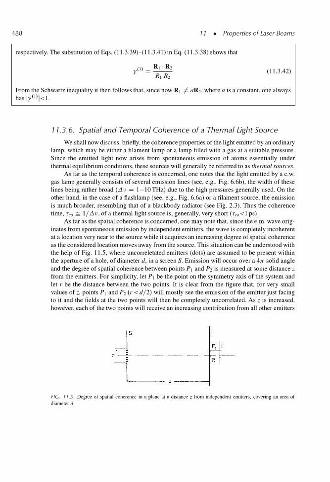
488 11 � Properties of Laser Beams
respectively. The substitution of Eqs. (11.3.39)–(11.3.41) in Eq. (11.3.38) shows that
� .1/ D R1 � R2
R1 R2(11.3.42)
From the Schwartz inequality it then follows that, since now R1 ¤ aR2, where a is a constant, one alwayshas j� .1/j<1.
11.3.6. Spatial and Temporal Coherence of a Thermal Light Source
We shall now discuss, briefly, the coherence properties of the light emitted by an ordinarylamp, which may be either a filament lamp or a lamp filled with a gas at a suitable pressure.Since the emitted light now arises from spontaneous emission of atoms essentially underthermal equilibrium conditions, these sources will generally be referred to as thermal sources.
As far as the temporal coherence is concerned, one notes that the light emitted by a c.w.gas lamp generally consists of several emission lines (see, e.g., Fig. 6.6b), the width of theselines being rather broad .� D 1�10 THz/ due to the high pressures generally used. On theother hand, in the case of a flashlamp (see, e.g., Fig. 6.6a) or a filament source, the emissionis much broader, resembling that of a blackbody radiator (see Fig. 2.3). Thus the coherencetime, �co Š 1=�, of a thermal light source is, generally, very short .�co<1 ps/.
As far as the spatial coherence is concerned, one may note that, since the e.m. wave orig-inates from spontaneous emission by independent emitters, the wave is completely incoherentat a location very near to the source while it acquires an increasing degree of spatial coherenceas the considered location moves away from the source. This situation can be understood withthe help of Fig. 11.5, where uncorreletated emitters (dots) are assumed to be present withinthe aperture of a hole, of diameter d, in a screen S. Emission will occur over a 4 solid angleand the degree of spatial coherence between points P1 and P2 is measured at some distance zfrom the emitters. For simplicity, let P1 be the point on the symmetry axis of the system andlet r be the distance between the two points. It is clear from the figure that, for very smallvalues of z, points P1 and P2 .r< d=2/ will mostly see the emission of the emitter just facingto it and the fields at the two points will then be completely uncorrelated. As z is increased,however, each of the two points will receive an increasing contribution from all other emitters
FIG. 11.5. Degree of spatial coherence in a plane at a distance z from independent emitters, covering an area ofdiameter d.
11.4 � Directionality 489
and the fields at the two points will become more and more correlated. A calculation of thedegree of spatial coherence, j� .1/j, as a function of the coordinate r is beyond the scope ofthis book and we refer elsewhere for this treatment..4/ We limit ourselves to pointing out thatj� .1/j turns out to be a function of the dimensionless quantity .rd=�z/ and, as an example, onehas j� .1/j D 0.88 for
r Š 0.16.�z=d/ (11.3.43)
a result which will be used in a following section.
11.4. DIRECTIONALITY
There are usually two ways by which the directionality, i.e., the divergence, of a laserbeam, or more generally of any light source, can be measured, namely: (i) By measuring thedegree of beam spreading at very large distances from the source. In fact, if we let W representa suitably defined radius of the beam at a very large distance z, the half-angle beam divergencecan be obtained from the relation
d D W=z (11.4.1)
(ii) By measuring the radial intensity distribution, I.r/, of the focused beam in the focal planeof a lens. To understand the basis of the latter measurement, let r be the coordinate of ageneral point in this focal plane, relative to an origin at the beam center. According to thediscussion made in relation to Fig. 1.8, the beam can be thought of as composed of a set ofplane waves propagating along slightly different directions..5/ The wave inclined at an angle to the propagation axis will then be focused, in the focal plane, to the point of radial coordinater given by (for small )
r D f (11.4.2)
Hence, a knowledge of the intensity distribution I.r/ in the focal plane of a lens gives theangular distribution of the original beam. In what follows, we will use either one of the abovemethods, as convenient.
The directional properties of a laser beam are strictly related to its spatial coherence. Wewill therefore discuss first the case of an e.m. wave with perfect spatial coherence and thenthe case of partial spatial coherence.
11.4.1. Beams with Perfect Spatial Coherence
Let us first consider a beam with perfect spatial coherence consisting of a plane wavefront of circular cross section, with diameter D, and constant amplitude over this cross section.Following the discussion above, the beam divergence can be calculated from a knowledge ofthe intensity distribution, I.r/, in the focal plane of a lens. This calculation was performed in
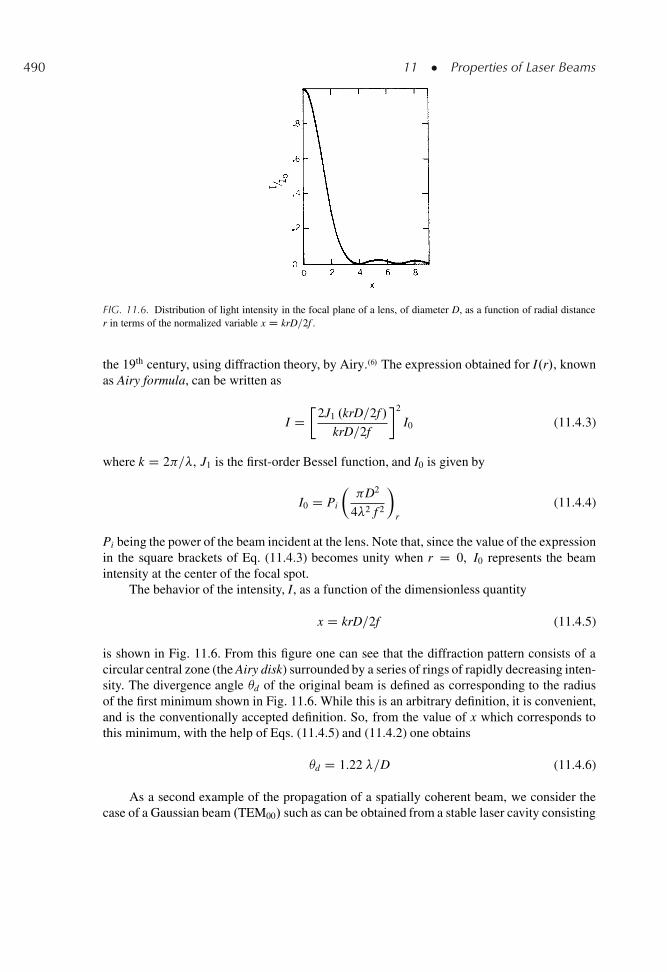
490 11 � Properties of Laser Beams
FIG. 11.6. Distribution of light intensity in the focal plane of a lens, of diameter D, as a function of radial distancer in terms of the normalized variable x D krD=2f .
the 19th century, using diffraction theory, by Airy..6/ The expression obtained for I.r/, knownas Airy formula, can be written as
I D�
2J1 .krD=2f /
krD=2f
�2
I0 (11.4.3)
where k D 2 =�, J1 is the first-order Bessel function, and I0 is given by
I0 D Pi
� D2
4�2 f 2
�r
(11.4.4)
Pi being the power of the beam incident at the lens. Note that, since the value of the expressionin the square brackets of Eq. (11.4.3) becomes unity when r D 0, I0 represents the beamintensity at the center of the focal spot.
The behavior of the intensity, I, as a function of the dimensionless quantity
x D krD=2f (11.4.5)
is shown in Fig. 11.6. From this figure one can see that the diffraction pattern consists of acircular central zone (the Airy disk) surrounded by a series of rings of rapidly decreasing inten-sity. The divergence angle d of the original beam is defined as corresponding to the radiusof the first minimum shown in Fig. 11.6. While this is an arbitrary definition, it is convenient,and is the conventionally accepted definition. So, from the value of x which corresponds tothis minimum, with the help of Eqs. (11.4.5) and (11.4.2) one obtains
d D 1.22 �=D (11.4.6)
As a second example of the propagation of a spatially coherent beam, we consider thecase of a Gaussian beam .TEM00/ such as can be obtained from a stable laser cavity consisting
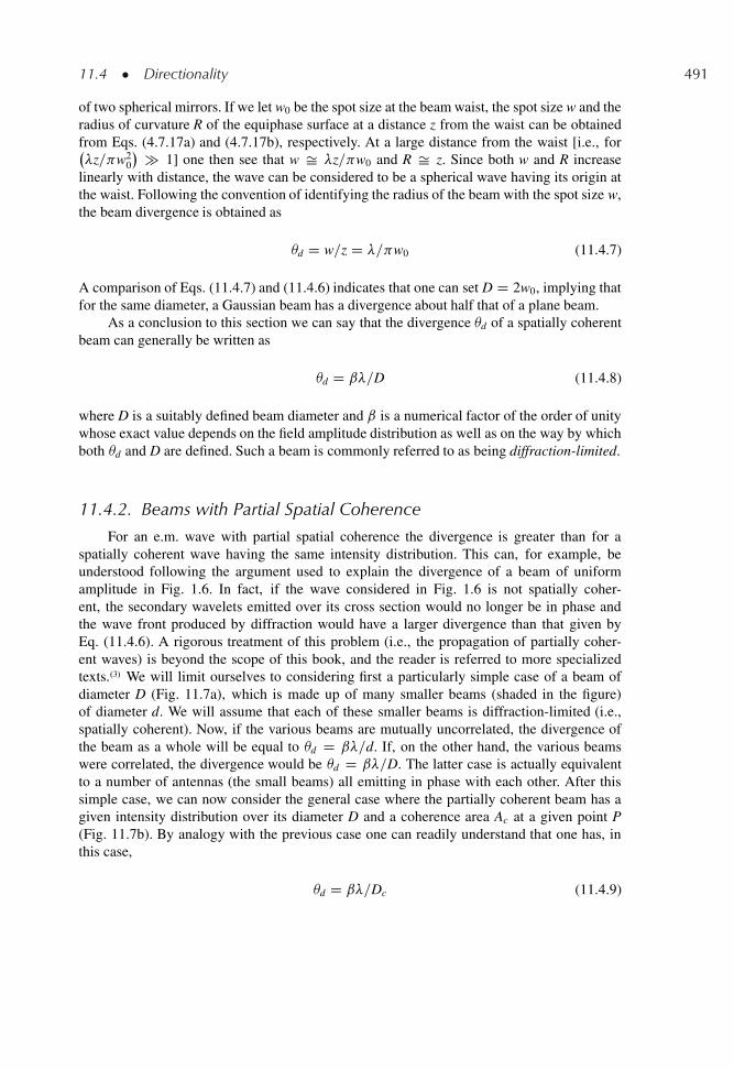
11.4 � Directionality 491
of two spherical mirrors. If we let w0 be the spot size at the beam waist, the spot size w and theradius of curvature R of the equiphase surface at a distance z from the waist can be obtainedfrom Eqs. (4.7.17a) and (4.7.17b), respectively. At a large distance from the waist [i.e., for�z= w2
0
� � 1] one then see that w Š �z= w0 and R Š z. Since both w and R increaselinearly with distance, the wave can be considered to be a spherical wave having its origin atthe waist. Following the convention of identifying the radius of the beam with the spot size w,the beam divergence is obtained as
d D w=z D �= w0 (11.4.7)
A comparison of Eqs. (11.4.7) and (11.4.6) indicates that one can set D D 2w0, implying thatfor the same diameter, a Gaussian beam has a divergence about half that of a plane beam.
As a conclusion to this section we can say that the divergence d of a spatially coherentbeam can generally be written as
d D ˇ�=D (11.4.8)
where D is a suitably defined beam diameter and ˇ is a numerical factor of the order of unitywhose exact value depends on the field amplitude distribution as well as on the way by whichboth d and D are defined. Such a beam is commonly referred to as being diffraction-limited.
11.4.2. Beams with Partial Spatial Coherence
For an e.m. wave with partial spatial coherence the divergence is greater than for aspatially coherent wave having the same intensity distribution. This can, for example, beunderstood following the argument used to explain the divergence of a beam of uniformamplitude in Fig. 1.6. In fact, if the wave considered in Fig. 1.6 is not spatially coher-ent, the secondary wavelets emitted over its cross section would no longer be in phase andthe wave front produced by diffraction would have a larger divergence than that given byEq. (11.4.6). A rigorous treatment of this problem (i.e., the propagation of partially coher-ent waves) is beyond the scope of this book, and the reader is referred to more specializedtexts..3/ We will limit ourselves to considering first a particularly simple case of a beam ofdiameter D (Fig. 11.7a), which is made up of many smaller beams (shaded in the figure)of diameter d. We will assume that each of these smaller beams is diffraction-limited (i.e.,spatially coherent). Now, if the various beams are mutually uncorrelated, the divergence ofthe beam as a whole will be equal to d D ˇ�=d. If, on the other hand, the various beamswere correlated, the divergence would be d D ˇ�=D. The latter case is actually equivalentto a number of antennas (the small beams) all emitting in phase with each other. After thissimple case, we can now consider the general case where the partially coherent beam has agiven intensity distribution over its diameter D and a coherence area Ac at a given point P(Fig. 11.7b). By analogy with the previous case one can readily understand that one has, inthis case,
d D ˇ�=Dc (11.4.9)
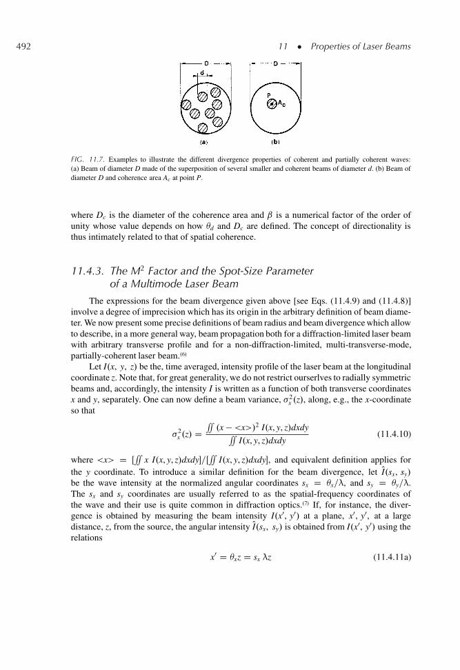
492 11 � Properties of Laser Beams
FIG. 11.7. Examples to illustrate the different divergence properties of coherent and partially coherent waves:(a) Beam of diameter D made of the superposition of several smaller and coherent beams of diameter d. (b) Beam ofdiameter D and coherence area Ac at point P.
where Dc is the diameter of the coherence area and ˇ is a numerical factor of the order ofunity whose value depends on how d and Dc are defined. The concept of directionality isthus intimately related to that of spatial coherence.
11.4.3. The M2 Factor and the Spot-Size Parameterof a Multimode Laser Beam
The expressions for the beam divergence given above [see Eqs. (11.4.9) and (11.4.8)]involve a degree of imprecision which has its origin in the arbitrary definition of beam diame-ter. We now present some precise definitions of beam radius and beam divergence which allowto describe, in a more general way, beam propagation both for a diffraction-limited laser beamwith arbitrary transverse profile and for a non-diffraction-limited, multi-transverse-mode,partially-coherent laser beam..6/
Let I.x, y, z/ be the, time averaged, intensity profile of the laser beam at the longitudinalcoordinate z. Note that, for great generality, we do not restrict ourserlves to radially symmetricbeams and, accordingly, the intensity I is written as a function of both transverse coordinatesx and y, separately. One can now define a beam variance, �2
x .z/, along, e.g., the x-coordinateso that
�2x .z/ D
’.x � <x>/2 I.x, y, z/dxdy’
I.x, y, z/dxdy(11.4.10)
where <x> D Œ’
x I.x, y, z/dxdy�=Œ’
I.x, y, z/dxdy�, and equivalent definition applies forthe y coordinate. To introduce a similar definition for the beam divergence, let OI.sx, sy/
be the wave intensity at the normalized angular coordinates sx D x=λ, and sy D y=λ.The sx and sy coordinates are usually referred to as the spatial-frequency coordinates ofthe wave and their use is quite common in diffraction optics..7/ If, for instance, the diver-gence is obtained by measuring the beam intensity I.x0, y0/ at a plane, x0, y0, at a largedistance, z, from the source, the angular intensity OI.sx, sy/ is obtained from I.x0, y0/ using therelations
x0 D xz D sx λz (11.4.11a)
11.4 � Directionality 493
and
y0 D yz D syλz (11.4.11b)
Having defined the intensity OI.sx, sy/, the variance of the spatial frequency sx can now bereadily defined as
�2sx
D’.sx � <sx>/
2 OI.sx, sy/dsxdsy’ OI.sx, sy/dsxdsy
(11.4.12)
where <sx> D Œ’
sxOI.sx, sy/dsxdsy�=Œ’ OI.sx, sy/dsxdsy�, and similarly for the y-coordinate. If
we now let u.x, y, z/ be the transverse amplitude profile of the beam (so that I / juj2) andOu.sx, sy/ be the spatial-frequency profile (so that OI / jOuj2/, we know that, for any arbitraryoptical beam, the two functions are related through a Fourier transform..8/ For any arbitraryreal laser beam, one can then prove that �2
x .z/ obeys the free space propagation equation
� 2x.z/ D � 2
x0 C � 2� 2sx.z � z0x/
2 (11.4.13)
where �x0 is the minimum value of �x and z0x is the coordinate at which this minimum isattained. One can also show from the same treatment that [compare with Eq. (11.3.28)]
�x0�sx 1=4 (11.4.14)
the equality holding only for a coherent Gaussian beam. In this case, in fact, one hasI.x, y, z/ / expŒ�2.x2 C y2/=w2.z/� while it can be readily shown, using the coordinate trans-formations Eq. (11.4.11), that OI.sx, sy/ / exp
��2 2w20
s2
x C s2y
�. From Eqs. (11.4.10) and
(11.4.12) one then gets
�x.z/ D w.z/=2 (11.4.15a)
�sx D 1=2 w0 (11.4.15b)
and obviously, setting z D 0 in (11.4.15a),
�x0 D w0=2 (11.4.15c)
From Eqs. (11.4.15b) and (11.4.15c) one then obtains
.�x0�sx/G D 1=4 (11.4.16)
Following the previous argument one can now define an M2x factor as the ratio between
the .�x0�sx/ product of the beam and the corresponding product, .�x0�sx/G, for a Gaussianbeam i.e.,
M2x D .�x0�sx/=.�x0�sx/G D 4 .�x0�sx/ (11.4.17)
494 11 � Properties of Laser Beams
and similarly for the y-coordinate. Note that, according to Eq. (11.4.14) one has M2x 1. The
term M2x is usually referred to as the beam quality. Since larger values of M2
x correspond tolower beam quality, it has also been referred to (less commonly) as the inverse beam qualityfactor. Note also that, if a comparison is made with a Gaussian beam having the same variance,i.e., if .�x0/G D .�x0/, M2
x then specifies how much the beam divergence exceeds that of aGaussian beam.
An alternative way to Eq. (11.4.13) for describing the propagation of a multimode laserbeam can be obtained by noting that, for a Gaussian beam, according to Eqs. (11.4.15a) and(11.4.15c) one has wx.z/ D 2�x.z/ and wx0 D 2�x0. Consequently, for a laser beam of generaltransverse profile, one can define the spot-size parameters Wx.z/ and Wx0 as
Wx.z/ D 2�x.z/ (11.4.18a)
Wx0 D 2�x0 (11.4.18b)
Note that we are using the upper-case symbols Wx.z/ and Wx0 to indicate the spot-size param-eters of an arbitrary laser beam. The substitution, in Eq. (11.4.13), of �x.z/ and �x0 fromEqs. (11.4.18) and of �sx from Eq. (11.4.17) then gives
W2x .z/ D W2
x0 C M4x
�2
2W2x0
.z � z0x/2 (11.4.19)
For a Gaussian beam, one obviously has Wx.z/ D wx.z/, Wx0 D wx0, and M2x D 1 and
Eq. (11.4.19) reduces to Eq. (4.7.13a). For a multimode laser beam, on the other hand,Eq. (11.4.19) represents an equation formally similar to that of a Gaussian beam except thatthe second term on the right hand side, expressing the spreading due to beam diffraction, ismultiplied by a factor M4
x .Equation (11.4.19) expresses the propagation of a multimode laser beam as a function of
a precisely defined spot-size parameter Wx.z/. Note that the beam propagation is determinedby the three parameters Wx0, M2
x and z0x. Their values can in principle be determined byperforming a measurement of the beam size Wx.z/ at three different z-coordinates. Note alsothat, at large distances from the waist position, z0x, one obtains from Eq. (11.4.19) Wx.z/ ŠM2
x�= Wx0�.z� z0x/. For a multimode laser beam, one can then define a beam divergence as
dx D Wx.z/=.z � z0x/ D M2x .�= Wx0/ (11.4.20)
The beam divergence of a multimode laser beam is thus M2x times that of a Gaussian beam
of the same spot size (i.e., such that wx0 D Wx0). A comparison of Eq. (11.4.20) withEq. (11.4.9) also allows one to establish a relation between M2
x , Wx0 and the diameter Dc
of the coherence area.
Example 11.4. M2-factor and spot-size parameter of a broad area semiconductor laser. We will considera broad area AlGaAs/GaAs semiconductor laser with output beam dimensions, at the exit face of thelaser i.e., in the near-field, of d? D 0.8�m and dk D 100�m and with beam divergences ? D 20ı andk D 10ı. The labels ? and k represent directions perpendicular and parallel to the junction plane, respec-tively. The diameters, d, are measured between the half-intensity points and, likewise, the divergences, ,
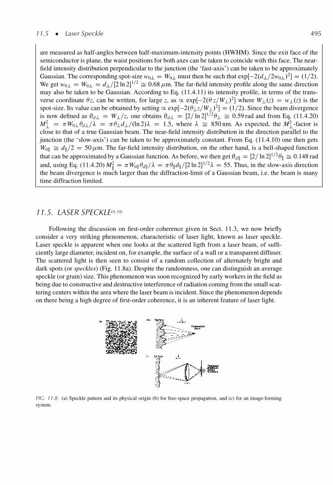
11.5 � Laser Speckle 495
are measured as half-angles between half-maximum-intensity points (HWHM). Since the exit face of thesemiconductor is plane, the waist positions for both axes can be taken to coincide with this face. The near-field intensity distribution perpendicular to the junction (the ‘fast-axis’) can be taken to be approximatelyGaussian. The corresponding spot-size w0? D W0? must then be such that expŒ�2.d?=2w0?/2� D .1=2/.We get w0? D W0? D d?=Œ2 ln 2�1=2 Š 0.68�m. The far-field intensity profile along the same directionmay also be taken to be Gaussian. According to Eq. (11.4.11) its intensity profile, in terms of the trans-verse coordinate z, can be written, for large z, as / expŒ�2. z=W?/2� where W?.z/ D w?.z/ is thespot-size. Its value can be obtained by setting / expŒ�2.?z=W?/2� D .1=2/. Since the beam divergenceis now defined as θd? D W?=z, one obtains θd? D Œ2= ln 2�1=2? Š 0.59 rad and from Eq. (11.4.20)M2
? D W0?d?=� D ?d?=.ln 2/� D 1.5, where � Š 850 nm. As expected, the M2?-factor is
close to that of a true Gaussian beam. The near-field intensity distribution in the direction parallel to thejunction (the ‘slow-axis’) can be taken to be approximately constant. From Eq. (11.4.10) one then getsW0k Š dk=2 D 50�m. The far-field intensity distribution, on the other hand, is a bell-shaped functionthat can be approximated by a Gaussian function. As before, we then get θdk D Œ2= ln 2�1=2k Š 0.148 radand, using Eq. (11.4.20) M2
k D W0kdk=� D kdk=Œ2 ln 2�1=2� D 55. Thus, in the slow-axis directionthe beam divergence is much larger than the diffraction-limit of a Gaussian beam, i.e. the beam is manytime diffraction limited.
11.5. LASER SPECKLE.9,10/
Following the discussion on first-order coherence given in Sect. 11.3, we now brieflyconsider a very striking phenomenon, characteristic of laser light, known as laser speckle.Laser speckle is apparent when one looks at the scattered ligth from a laser beam, of suffi-ciently large diameter, incident on, for example, the surface of a wall or a transparent diffuser.The scattered light is then seen to consist of a random collection of alternately bright anddark spots (or speckles) (Fig. 11.8a). Despite the randomness, one can distinguish an averagespeckle (or grain) size. This phenomenon was soon recognized by early workers in the field asbeing due to constructive and destructive interference of radiation coming from the small scat-tering centers within the area where the laser beam is incident. Since the phenomenon dependson there being a high degree of first-order coherence, it is an inherent feature of laser light.
FIG. 11.8. (a) Speckle pattern and its physical origin (b) for free-space propagation, and (c) for an image-formingsystem.
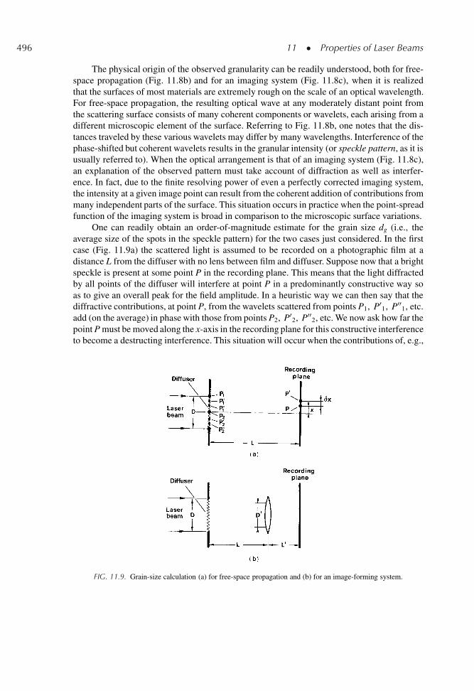
496 11 � Properties of Laser Beams
The physical origin of the observed granularity can be readily understood, both for free-space propagation (Fig. 11.8b) and for an imaging system (Fig. 11.8c), when it is realizedthat the surfaces of most materials are extremely rough on the scale of an optical wavelength.For free-space propagation, the resulting optical wave at any moderately distant point fromthe scattering surface consists of many coherent components or wavelets, each arising from adifferent microscopic element of the surface. Referring to Fig. 11.8b, one notes that the dis-tances traveled by these various wavelets may differ by many wavelengths. Interference of thephase-shifted but coherent wavelets results in the granular intensity (or speckle pattern, as it isusually referred to). When the optical arrangement is that of an imaging system (Fig. 11.8c),an explanation of the observed pattern must take account of diffraction as well as interfer-ence. In fact, due to the finite resolving power of even a perfectly corrected imaging system,the intensity at a given image point can result from the coherent addition of contributions frommany independent parts of the surface. This situation occurs in practice when the point-spreadfunction of the imaging system is broad in comparison to the microscopic surface variations.
One can readily obtain an order-of-magnitude estimate for the grain size dg (i.e., theaverage size of the spots in the speckle pattern) for the two cases just considered. In the firstcase (Fig. 11.9a) the scattered light is assumed to be recorded on a photographic film at adistance L from the diffuser with no lens between film and diffuser. Suppose now that a brightspeckle is present at some point P in the recording plane. This means that the light diffractedby all points of the diffuser will interfere at point P in a predominantly constructive way soas to give an overall peak for the field amplitude. In a heuristic way we can then say that thediffractive contributions, at point P, from the wavelets scattered from points P1, P0
1, P001, etc.
add (on the average) in phase with those from points P2, P02, P00
2, etc. We now ask how far thepoint P must be moved along the x-axis in the recording plane for this constructive interferenceto become a destructing interference. This situation will occur when the contributions of, e.g.,
FIG. 11.9. Grain-size calculation (a) for free-space propagation and (b) for an image-forming system.
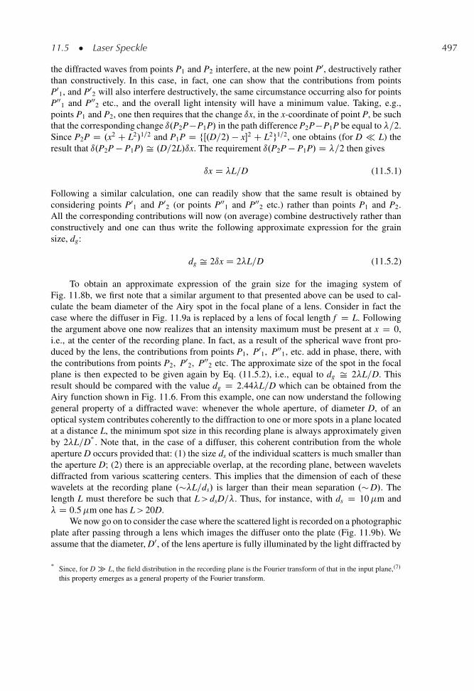
11.5 � Laser Speckle 497
the diffracted waves from points P1 and P2 interfere, at the new point P0, destructively ratherthan constructively. In this case, in fact, one can show that the contributions from pointsP0
1, and P02 will also interfere destructively, the same circumstance occurring also for points
P001 and P00
2 etc., and the overall light intensity will have a minimum value. Taking, e.g.,points P1 and P2, one then requires that the change ıx, in the x-coordinate of point P, be suchthat the corresponding change ı.P2P�P1P/ in the path difference P2P�P1P be equal to �=2.Since P2P D .x2 C L2/1=2 and P1P D fŒ.D=2/ � x�2 C L2g1=2, one obtains (for D � L) theresult that ı.P2P � P1P/ Š .D=2L/ıx. The requirement ı.P2P � P1P/ D �=2 then gives
ıx D �L=D (11.5.1)
Following a similar calculation, one can readily show that the same result is obtained byconsidering points P0
1 and P02 (or points P00
1 and P002 etc.) rather than points P1 and P2.
All the corresponding contributions will now (on average) combine destructively rather thanconstructively and one can thus write the following approximate expression for the grainsize, dg:
dg Š 2ıx D 2�L=D (11.5.2)
To obtain an approximate expression of the grain size for the imaging system ofFig. 11.8b, we first note that a similar argument to that presented above can be used to cal-culate the beam diameter of the Airy spot in the focal plane of a lens. Consider in fact thecase where the diffuser in Fig. 11.9a is replaced by a lens of focal length f D L. Followingthe argument above one now realizes that an intensity maximum must be present at x D 0,i.e., at the center of the recording plane. In fact, as a result of the spherical wave front pro-duced by the lens, the contributions from points P1, P0
1, P001, etc. add in phase, there, with
the contributions from points P2, P02, P00
2 etc. The approximate size of the spot in the focalplane is then expected to be given again by Eq. (11.5.2), i.e., equal to dg Š 2�L=D. Thisresult should be compared with the value dg D 2.44�L=D which can be obtained from theAiry function shown in Fig. 11.6. From this example, one can now understand the followinggeneral property of a diffracted wave: whenever the whole aperture, of diameter D, of anoptical system contributes coherently to the diffraction to one or more spots in a plane locatedat a distance L, the minimum spot size in this recording plane is always approximately givenby 2�L=D
�
. Note that, in the case of a diffuser, this coherent contribution from the wholeaperture D occurs provided that: (1) the size ds of the individual scatters is much smaller thanthe aperture D; (2) there is an appreciable overlap, at the recording plane, between waveletsdiffracted from various scattering centers. This implies that the dimension of each of thesewavelets at the recording plane .��L=ds/ is larger than their mean separation .� D/. Thelength L must therefore be such that L> dsD=�. Thus, for instance, with ds D 10�m and� D 0.5�m one has L> 20D.
We now go on to consider the case where the scattered light is recorded on a photographicplate after passing through a lens which images the diffuser onto the plate (Fig. 11.9b). Weassume that the diameter, D0, of the lens aperture is fully illuminated by the light diffracted by
�Since, for D � L, the field distribution in the recording plane is the Fourier transform of that in the input plane,.7/
this property emerges as a general property of the Fourier transform.
498 11 � Properties of Laser Beams
each individual scatterer, i.e., that .2�L=ds/ D0. Given this condition, the whole aperturecontributes via diffraction to each spot on the photographic plate and the grain size, dg, at theplate is given by
dg D 2�L0=D0 (11.5.3)
Example 11.5. Grain size of the speckle pattern asseen by a human observer. We will consider a red,�D 633 nm, He-Ne laser beam illuminating, e.g., an areaof diameter D D 2 cm on a scattering surface for whichthe individual scatterers are taken to have a dimensionds D 50 μm. The scattered ligth is observed by a humaneye at a distance L D 50 cm from the diffuser. We will takeL0 D 2 cm as the distance between the retina and the lensof the eye and assume a pupil diameter D0 D 2 mm. Since.2�L=ds/ Š 12.7 mm is much greater than D0, the wholeaperture of the eye is illuminated by the light diffractedby each individual scatterer. The apparent size of thespeckle at the illuminated region of diffuser is obtainedfrom Eq. (11.5.4) as dag Š 316 μm. Note that, if theobserver moves to a distance L D 100 cm from the dif-fuser, the apparent grain-size on the D D 2 cm illuminatedspot of the diffuser will double to � 632 μm.
It should be noted that the arrangement ofFig. 11.9b also corresponds to the case whereone looks directly at a scattering surface. Inthis case the lens and the recording plane cor-respond to the lens of the eye and the retina,respectively. Accordingly, dg, as given byEq. (11.5.3), can be taken as the expressionfor the grain size on the retina. Note that theapparent grain size on the scattering surface,dag, is dg.L=L0/ so that
dag D 2�L=D0 (11.5.4)
This expression, which actually gives theeye’s resolution for objects at a distance L,shows that dag is expected to increase withincreasing L, i.e., with increasing distancebetween the observer and the diffuser andto decrease with increasing aperture of the
iris (i.e., when the eye is dark-adapted). Both these predictions are readily confirmed byexperimental observations.
Speckle noise often constitutes an undesirable feature of coherent light. The spatial reso-lution of the image of an object made via illumination with laser light is in fact often limited byspeckle noise. Speckle noise is also apparent in the reconstructed image of a hologram, againlimiting the spatial resolution of this image. Some techniques have therefore been developedto reduce speckle from coherently illuminated objects..10/ Speckle noise is not always a nui-sance, however. In fact techniques have been developed that exploit the presence of speckle toshow up, in a rather simple way, the deformation of large objects arising, e.g., from stressesor vibrations (speckle interferometry).
11.6. BRIGHTNESS
The brightness B of a light source or of a laser source has already been introduced inSect. 1.4.4. [see Eqs. (1.4.3) and (1.4.4)]. We note again that the most significant parameterof a laser beam (and in general of any light source) is not simply its power or its intensity,but its brightness. This was already pointed out in Sect. 1.4.4. where it was shown that themaximum peak intensity, which can be obtained by focusing a given beam, is proportional tothe beam brightness [see Eq. (1.4.6)]. This is further emphasized by the fact that, although theintensity of a beam can be increased, its brightness cannot. In fact, the simple arrangementof confocal lenses shown in Fig. 11.10 can be used to decrease the beam diameter, if f2<f1,
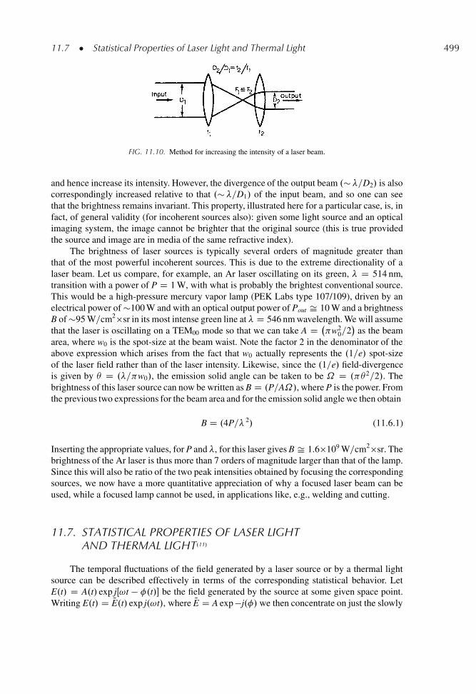
11.7 � Statistical Properties of Laser Light and Thermal Light 499
FIG. 11.10. Method for increasing the intensity of a laser beam.
and hence increase its intensity. However, the divergence of the output beam .��=D2/ is alsocorrespondingly increased relative to that .��=D1/ of the input beam, and so one can seethat the brightness remains invariant. This property, illustrated here for a particular case, is, infact, of general validity (for incoherent sources also): given some light source and an opticalimaging system, the image cannot be brighter that the original source (this is true providedthe source and image are in media of the same refractive index).
The brightness of laser sources is typically several orders of magnitude greater thanthat of the most powerful incoherent sources. This is due to the extreme directionality of alaser beam. Let us compare, for example, an Ar laser oscillating on its green, � D 514 nm,transition with a power of P D 1 W, with what is probably the brightest conventional source.This would be a high-pressure mercury vapor lamp (PEK Labs type 107/109), driven by anelectrical power of �100 W and with an optical output power of Pout Š 10 W and a brightnessB of �95 W=cm2�sr in its most intense green line at � D 546 nm wavelength. We will assumethat the laser is oscillating on a TEM00 mode so that we can take A D
w20=2
�as the beam
area, where w0 is the spot-size at the beam waist. Note the factor 2 in the denominator of theabove expression which arises from the fact that w0 actually represents the .1=e/ spot-sizeof the laser field rather than of the laser intensity. Likewise, since the .1=e/ field-divergenceis given by D .�= w0/, the emission solid angle can be taken to be ˝ D . 2=2/. Thebrightness of this laser source can now be written as B D .P=A˝/, where P is the power. Fromthe previous two expressions for the beam area and for the emission solid angle we then obtain
B D .4P=� 2/ (11.6.1)
Inserting the appropriate values, for P and �, for this laser gives B Š 1.6�109 W=cm2�sr. Thebrightness of the Ar laser is thus more than 7 orders of magnitude larger than that of the lamp.Since this will also be ratio of the two peak intensities obtained by focusing the correspondingsources, we now have a more quantitative appreciation of why a focused laser beam can beused, while a focused lamp cannot be used, in applications like, e.g., welding and cutting.
11.7. STATISTICAL PROPERTIES OF LASER LIGHTAND THERMAL LIGHT.11/
The temporal fluctuations of the field generated by a laser source or by a thermal lightsource can be described effectively in terms of the corresponding statistical behavior. LetE.t/ D A.t/ exp jŒ!t � �.t/� be the field generated by the source at some given space point.Writing E.t/ D QE.t/ exp j.!t/, where QE D A exp �j.�/ we then concentrate on just the slowly
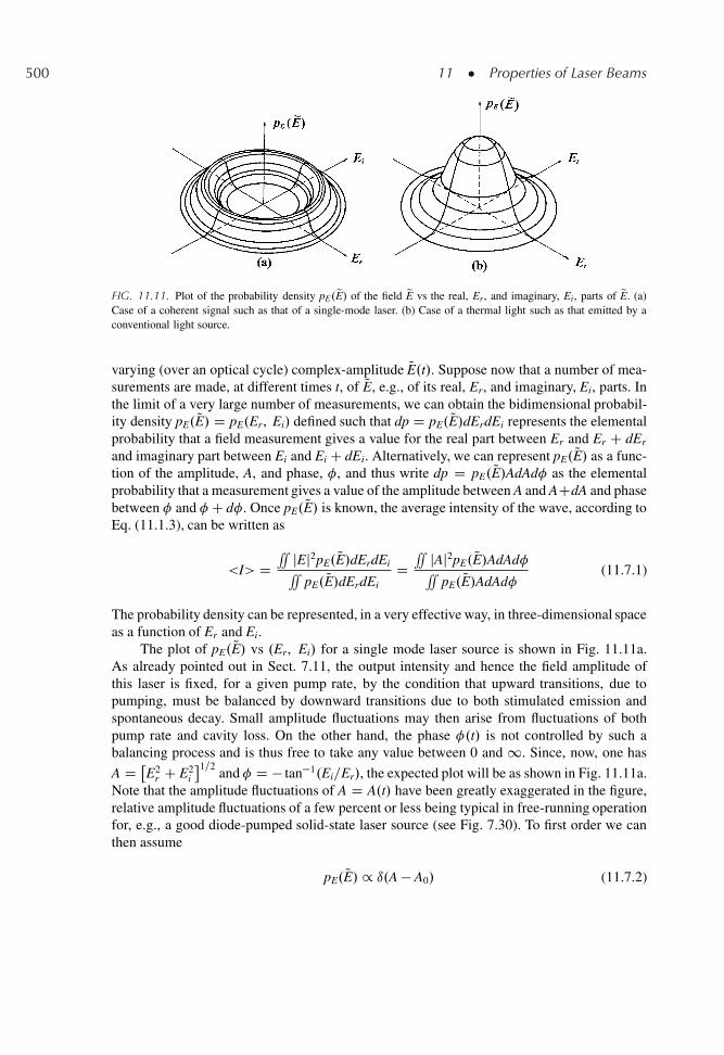
500 11 � Properties of Laser Beams
FIG. 11.11. Plot of the probability density pE.QE/ of the field QE vs the real, Er, and imaginary, Ei, parts of QE. (a)Case of a coherent signal such as that of a single-mode laser. (b) Case of a thermal light such as that emitted by aconventional light source.
varying (over an optical cycle) complex-amplitude QE.t/. Suppose now that a number of mea-surements are made, at different times t, of QE, e.g., of its real, Er, and imaginary, Ei, parts. Inthe limit of a very large number of measurements, we can obtain the bidimensional probabil-ity density pE. QE/ D pE.Er, Ei/ defined such that dp D pE. QE/dErdEi represents the elementalprobability that a field measurement gives a value for the real part between Er and Er C dEr
and imaginary part between Ei and Ei C dEi. Alternatively, we can represent pE. QE/ as a func-tion of the amplitude, A, and phase, �, and thus write dp D pE. QE/AdAd� as the elementalprobability that a measurement gives a value of the amplitude between A and ACdA and phasebetween � and � C d�. Once pE. QE/ is known, the average intensity of the wave, according toEq. (11.1.3), can be written as
<I> D’ jEj2pE. QE/dErdEi’
pE. QE/dErdEiD’ jAj2pE. QE/AdAd�’
pE. QE/AdAd�(11.7.1)
The probability density can be represented, in a very effective way, in three-dimensional spaceas a function of Er and Ei.
The plot of pE. QE/ vs .Er, Ei/ for a single mode laser source is shown in Fig. 11.11a.As already pointed out in Sect. 7.11, the output intensity and hence the field amplitude ofthis laser is fixed, for a given pump rate, by the condition that upward transitions, due topumping, must be balanced by downward transitions due to both stimulated emission andspontaneous decay. Small amplitude fluctuations may then arise from fluctuations of bothpump rate and cavity loss. On the other hand, the phase �.t/ is not controlled by such abalancing process and is thus free to take any value between 0 and 1. Since, now, one has
A D �E2
r C E2i
1=2and � D � tan�1.Ei=Er/, the expected plot will be as shown in Fig. 11.11a.
Note that the amplitude fluctuations of A D A.t/ have been greatly exaggerated in the figure,relative amplitude fluctuations of a few percent or less being typical in free-running operationfor, e.g., a good diode-pumped solid-state laser source (see Fig. 7.30). To first order we canthen assume
pE. QE/ / ı.A � A0/ (11.7.2)
11.8 � Comparison Between Laser Light and Thermal Light 501
where A0 is a constant determined by the average intensity value. The substitution ofEqs. (11.7.2) into (11.7.1) gives in fact <I> D A2
0. In the time domain, the point that rep-resents QE.t/ in the .Er, Ei/ plane will then travel essentially along the circumference of radiusj QEj D A0. As a consequence of the statistical nature of the phase fluctuations, this move-ment will be random and the corresponding angular speed, d�=dt, will establish the laserbandwidth.
The plot of pE. QE/ vs .Er, Ei/ for a thermal light source is shown in Fig. 11.11b. Inthis case, the field is due to the superposition of the uncorreleted light emitted, by sponta-neous emission, from the individual atoms of the light source. Since the number of theseemitters is very large, it follows from the central limit theorem of statistics that the proba-bility distribution of both real and imaginary parts of QE must follow a Gaussian law. We canthus write
pE. QE/ / exp ��
E2r C E2
i
A20
�D exp �
�A2
A20
�(11.7.3)
where A0 is a constant again determined by the average light intensity. The substitution ofEqs. (11.7.3) into (11.7.1) gives, in fact, <I> D A2
0. Note that the average values of bothEr and Ei are now zero. Thus, the time-domain movement of the point representing QE inthe .Er, Ei/ plane consists now of a random movement around the origin. The speed of thismovement in terms of both amplitude and phase (i.e., in term of both dA/Adt and d�=dt)establishes, in this case, the bandwidth of this thermal source.
11.8. COMPARISON BETWEEN LASER LIGHT AND THERMAL LIGHT
A comparison will now be made between a red-emitting, � D 633 nm, He-Ne laseroscillating, on a single mode, with a “modest” output power of 1 mW with what is probablythe brightest conventional source, already considered in Sect. 11.6. (PEK Labs type 107/109),giving an optical output power of Pout Š 10 W and a brightness B of �95 W=cm2 � sr inits most intense green line at � D 546 nm wavelength. To obtain a beam with good spatialcoherence from this lamp, one can use the arrangement of Fig. 11.12, where a lens of focallength, f , and suitable aperture, D, collects a fraction of the emitted light. The lamp is sim-ulated by individual emitters, located within an aperture, of diameter d, made in a screen S.Following the discussion in Sect. 11.3.6, to obtain a beam with a spatial coherence whichapproaches the ideal, the aperture D must be chosen so that [see Eq. (11.3.43)]
D Š 0.32�f=d (11.8.1)
This beam, although having a degree of spatial coherence somewhat less than unity[� .1/.P1, P2/ Š 0.88, in the case considered], may be regarded, generously, as having thesame degree of spatial coherence as that of the He-Ne laser [whose value for � .1/ may be takento be essentially unitary]. The output power of the beam obtained after the lens is then givenby Pout D BA˝ , where B is the brightness of the lamp, A is its emitting area .A D d2=4/ and˝ is the acceptance solid angle of the lens .˝ D 2D2=4f 2/. With the help of Eq. (11.8.1)
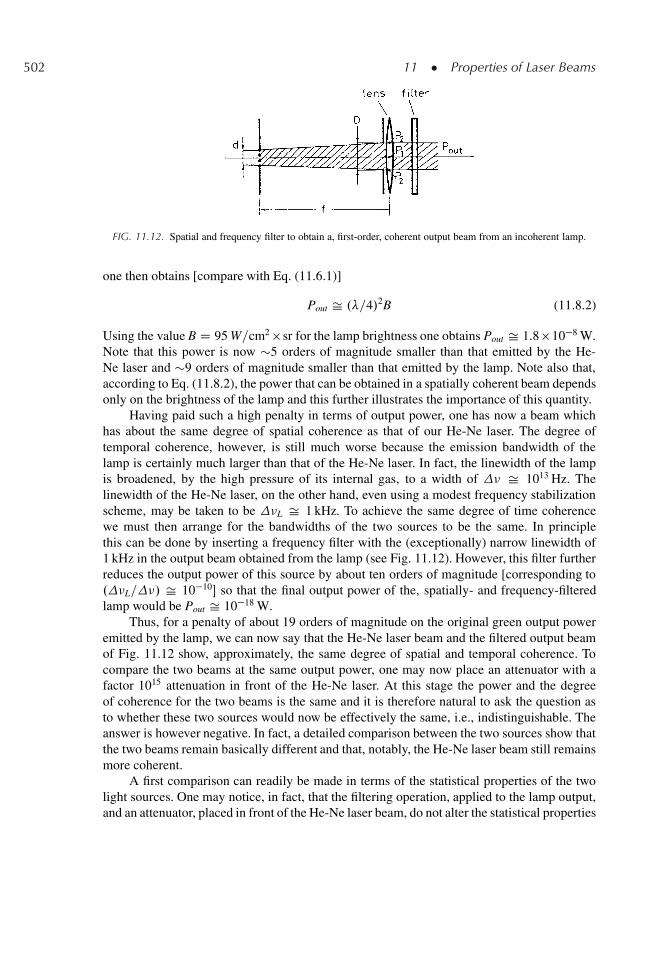
502 11 � Properties of Laser Beams
FIG. 11.12. Spatial and frequency filter to obtain a, first-order, coherent output beam from an incoherent lamp.
one then obtains [compare with Eq. (11.6.1)]
Pout Š .�=4/2B (11.8.2)
Using the value B D 95 W=cm2 � sr for the lamp brightness one obtains Pout Š 1.8 �10�8 W.Note that this power is now �5 orders of magnitude smaller than that emitted by the He-Ne laser and �9 orders of magnitude smaller than that emitted by the lamp. Note also that,according to Eq. (11.8.2), the power that can be obtained in a spatially coherent beam dependsonly on the brightness of the lamp and this further illustrates the importance of this quantity.
Having paid such a high penalty in terms of output power, one has now a beam whichhas about the same degree of spatial coherence as that of our He-Ne laser. The degree oftemporal coherence, however, is still much worse because the emission bandwidth of thelamp is certainly much larger than that of the He-Ne laser. In fact, the linewidth of the lampis broadened, by the high pressure of its internal gas, to a width of � Š 1013 Hz. Thelinewidth of the He-Ne laser, on the other hand, even using a modest frequency stabilizationscheme, may be taken to be �L Š 1 kHz. To achieve the same degree of time coherencewe must then arrange for the bandwidths of the two sources to be the same. In principlethis can be done by inserting a frequency filter with the (exceptionally) narrow linewidth of1 kHz in the output beam obtained from the lamp (see Fig. 11.12). However, this filter furtherreduces the output power of this source by about ten orders of magnitude [corresponding to.�L=�/ Š 10�10� so that the final output power of the, spatially- and frequency-filteredlamp would be Pout Š 10�18 W.
Thus, for a penalty of about 19 orders of magnitude on the original green output poweremitted by the lamp, we can now say that the He-Ne laser beam and the filtered output beamof Fig. 11.12 show, approximately, the same degree of spatial and temporal coherence. Tocompare the two beams at the same output power, one may now place an attenuator with afactor 1015 attenuation in front of the He-Ne laser. At this stage the power and the degreeof coherence for the two beams is the same and it is therefore natural to ask the question asto whether these two sources would now be effectively the same, i.e., indistinguishable. Theanswer is however negative. In fact, a detailed comparison between the two sources show thatthe two beams remain basically different and that, notably, the He-Ne laser beam still remainsmore coherent.
A first comparison can readily be made in terms of the statistical properties of the twolight sources. One may notice, in fact, that the filtering operation, applied to the lamp output,and an attenuator, placed in front of the He-Ne laser beam, do not alter the statistical properties
Problems 503
of the corresponding light. Thus Fig. 11.11a and Fig. 11.11b can still be used to describe thestatistical properties of the two sources and, from these figures, a first basic difference betweenthe two beams is now apparent. Note that, since the output powers of the two beams havebeen equalised, the quantity A0 appearing in Eqs. (11.7.2) and (11.7.3) is the same for the twosources. Note also that, if the degree of temporal coherence of the two beams is made equal,this simply means that the speed of movement of the point representing QE in the .Er, Ei/ planeis the same for the two cases. Note lastly that, if the degree of spatial coherence of the twobeams is equalised, this simply means that, for each beam, the movement in the .Er, Ei/ planewill be the same at any point of the wavefront. Nonetheless, the statistical properties of thetwo beams, as represented in Fig. 11.11, still remain fundamentally different.
A second comparison between the two sources can be made in terms of the coherenceproperties to higher-order (see Appendix H). To this purpose, we recall that the coherencefunction � .1/ was introduced in Sect. 11.3 in terms of the product E.x1/E�.x2/ between fieldstaken at two different space-time points xi D .ri, ti/. For this reason, a superscript (1) wasused for � as a reminder of the fact that one is actually performing a, first-order, correlationbetween the two fields. To higher order, one can in fact introduce a whole class of correla-tion functions, e.g., <E.x1/E.x2/E�.x3/E�.x4/> involving the four distinct space-time pointsx1, x2, x3, and x4, and so on to yet higher order
�
. One can then introduce some suitable defi-nition of a higher-order coherence, � .n/, in terms of these higher-order correlation functions.When this is done, it turns out that the higher-order coherence of our monomode laser sourceis still larger than the filtered beam taken from a lamp (see Appendix H). It also turns out that,fundamentally, one can at best arrange for the two sources to exhibit the same, first-order,coherence i.e., the same degree of spatial and temporal coherence, as indeed achieved by thefiltering system of Fig. 11.12.
Thus, as a conclusion, despite having paid such a heavy penalty in terms of output power,our filtered thermal source remains basically different from a laser.
PROBLEMS
11.1. Calculate � .1/.r1, r1, �/ for a sinusoidal wave.
11.2. Prove Eq. (11.3.9).
11.3. For the Michelson interferometer of Fig. 11.4a, find the analytical relation between the intensityalong the C direction, Ic, and � .1/.r, r, �/, where � D 2.L3 � L2/=c.
11.4. Assume that the field at point P of the Michelson interferometer of Fig. 11.4a is made of a sinu-soidal wave with constant amplitude and random phase jumps (see Fig. 2.9). Using the expressionfor � .1/.�/ calculated in Appendix B for this field and the relation between Ic and � .1/.�/
calculated in the previous problem, find the analytical expression of Vp D Vp.�/.
11.5. The shape of the spectral output of a CO2 laser beam operating at � D 10.6 μm is approximatelyGaussian with a bandwidth of 10 kHz Œ�L is defined according to Eq. (11.3.27)]. Calculate thecoherence length Lc and the distance L between two successive maxima of the intensity curveof Fig. 11.4b.
�Actually, it can be shown that a given field E.x/ can, in principle. be completely characterized by either the infiniteset of values for E obtained by changing x, or by the infinite set of correlation functions as indicated above.
504 11 � Properties of Laser Beams
11.6. A plane e.m. wave of circular cross section, uniform intensity, and perfect spatial coherenceis focused by a lens. What is the increase in intensity at the focus compared to that of theincident wave?
11.7. A Gaussian beam is focused by a lens of focal length f . Assuming that the waist of the incidentbeam is located at the lens position and that the corresponding spot-size w0 is appreciably smallerthan the lens diameter, relate the peak intensity at the focal spot to the power, Pi, of the incidentbeam. Compare then the resulting expression with Eq. (11.4.4).
11.8. The near-field transverse-intensity profile of a Nd:YAG laser beam, at � D 1.064 μm wavelength,is, to a good approximation, Gaussian with a diameter (FWHM) D Š 4 mm. The half-conebeam divergence, measured at the half-maximum point of the far-field intensity distribution, is dŠ 3 mrad. Calculate the corresponding M2 factor.
11.9. The near-field transverse intensity profile of a pulsed TEA CO2 laser beam, at � D 10.6 μmwavelength, is, to a good approximation, constant over its 1 cm � 4 cm dimension. The laser isadvertised to have a M2 factor of 16 along both axes. Assuming the waist position to be located atthe position of the output mirror, calculate the spot-size parameters at a distance from this mirrorof z D 3 m.
References
1. M. Born and E. Wolf, Principles of Optics, 6th edn. (Pergamon Press, Oxford, 1980), pp. 491–544.2. W. H. Louisell, Radiation and Noise in Quantum Electronics (McGraw-Hill, New York, 1964), pp. 47–53.3. A. Jeffrey, Handbook of Mathematical Formulas and Integrals (Academic, San Diego 1995) p. 244.4. Reference [1], pp. 508–518.5. J. W. Goodman, Introduction to Fourier Optics (McGraw-Hill, New York, 1968).6. Reference [1], pp. 395–398.7. A. E. Siegman, Defining and Measuring Laser Beam Quality, in Solid-State Lasers-New Developments
and Applications, ed. by M. Inguscio and R. Wallenstein (Plenum, New York, 1993) pp. 13–28.8. Reference [4], Chapter 5.9. Laser Speckle and Related Phenomena, ed. by J. C. Dainty (Springer-Verlag, Berlin 1975).
10. M. Francon, Laser Speckle and Applications in Optics (Academic, New York, 1979).11. R. J. Glauber, Optical Coherence and Photon Statistics, in Quantum Optics and Electronics, ed. by C. De Witt,
A. Blandin, and C. Cohen-Tannoudji (Gordon and Breach, New York, 1965), pp. 71, 94–98, 103, 151–155.
12
Laser Beam Transformation:Propagation, Amplification, FrequencyConversion, Pulse Compressionand Pulse Expansion
12.1. INTRODUCTION
Before it is put to use, a laser beam is generally transformed in some way. The mostcommon type of transformation is that which occurs when the beam is simply made to prop-agate in free space or through a suitable optical system. Since this produces a change in thespatial distribution of the beam (e.g., the beam may be focused or expanded), we shall refer tothis as a spatial transformation of the laser beam. A second type of transformation, also ratherfrequently encountered, is that which occurs when the beam is passed through an amplifier orchain of amplifiers. Since the main effect here is to alter the beam amplitude, we shall refer tothis as amplitude transformation. A third, rather different, case occurs when the wavelengthof the beam is changed as a result of propagating through a suitable nonlinear optical material(wavelength transformation or frequency conversion). Finally the temporal behavior of thelaser beam can be modified by a suitable optical element. For example, the amplitude of a cwlaser beam may be temporally modulated by an electro-optic or acousto-optic modulator orthe time duration of a laser pulse may be increased (pulse expansion) or decreased (pulse com-pression) using suitably dispersive optical systems or nonlinear optical elements. This fourthand last case will be referred to as time transformation. It should be noted that these fourtypes of beam transformation are often interrelated. For instance, amplitude transformationand frequency conversion often result in spatial and time transformations occurring as well.
In this chapter the four cases of laser beam transformation introduced above will bebriefly discussed. In the case of frequency conversion, of the various nonlinear optical effects
O. Svelto, Principles of Lasers,c
505DOI: 10.1007/978-1-4419-1302-9 12, � Springer Science+Business Media LLC 2010
506 12 � Propagation, Amplification, Frequency Conversion, Pulse Compression
that can be used.1/ to achieve this, only the so-called parametric effects will be consideredhere. These in fact provide some of the most useful techniques so far developed for producingnew sources of coherent light. Time transformation will be considered only for the cases ofpulse expansion or pulse compression, while we refer elsewhere for the case of amplitudemodulation..2/ We also omit a number of aspects of amplitude and time transformation thatarise from the nonlinear phenomenon of self-focusing and the associated phenomenon of self-phase-modulation,.3/ although it should be noted that they can play a very important role inlimiting, for instance, the performance of laser amplifiers.
12.2. SPATIAL TRANSFORMATION: PROPAGATIONOF A MULTIMODE LASER BEAM.4,5/
The free-space propagation of a Gaussian beam and of a multi-transverse-mode beam hasalready been considered in Sects. 4.7.2 and 11.4.3, respectively. In Sect. 4.7.2 it was shownthat a Gaussian beam, of, e.g., circular cross-section, is characterized by two parameters,namely the coordinate, z0, of the beam-waist and the corresponding spot-size, w0. By contrastto this, it was shown in Sect. 11.4.3 that a multi-mode beam, of, e.g., circular cross sectionagain, is characterized by three parameters, namely the coordinate, z0, of the beam-waist, thespot-size parameter W0, and M2, the beam-quality factor. The propagation of a Gaussian beamthrough a general optical system characterized by a given ABCD matrix, has, on the otherhand, been considered in Sect. 4.7.3. It was shown there that the complex q-parameter of thebeam, after passing through the optical system, can be readily obtained from the q-parameterof the input beam once the matrix elements, A, B, C, D, are known. To complete this picture,we will consider, in this Section, the propagation of a multi-mode laser beam through a generaloptical system characterized by a given ABCD matrix.
Consider first the free-space propagation of a multimode laser beam. The spot-sizeparameter, along, e.g., the transverse direction x and at a longitudinal coordinate z, is describedby Eq. (11.4.19) which, for convenience, is reproduced here
W2x .z/D W2
0x C M4x
� 2
2W20x
.z � z0x/2 (12.2.1)
We can now see that, as far as free-space propagation is concerned, the multimode laser beambehaves as if it contained an “embedded Gaussian beam” having the same waist location, z0x,as the multimode beam and a spot-size, at any coordinate z, given by
wx.z/D Wx.z/=Mx (12.2.2)
where Mx DpM2
x is a constant. In fact, the substitution of Eq. (12.2.2) in Eq. (12.2.1) readilygives Eq. (4.7.13a). It can also be shown that the radius of curvature, R.z/, of this embeddedGaussian beam equals, at any z, that of the multimode beam.
This notion of an embedded Gaussian beam can be shown to hold also for prop-agation through a general optical system described by, e.g., its ABCD matrix. Accord-ingly, the propagation of the multi-mode beam can be obtained by the following simple
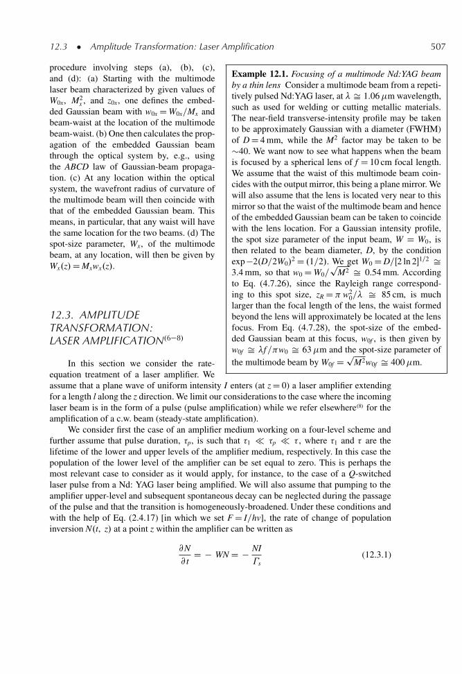
12.3 � Amplitude Transformation: Laser Amplification 507
Example 12.1. Focusing of a multimode Nd:YAG beamby a thin lens Consider a multimode beam from a repeti-tively pulsed Nd:YAG laser, at � Š 1.06�m wavelength,such as used for welding or cutting metallic materials.The near-field transverse-intensity profile may be takento be approximately Gaussian with a diameter (FWHM)of D D 4 mm, while the M2 factor may be taken to be�40. We want now to see what happens when the beamis focused by a spherical lens of f D 10 cm focal length.We assume that the waist of this multimode beam coin-cides with the output mirror, this being a plane mirror. Wewill also assume that the lens is located very near to thismirror so that the waist of the multimode beam and henceof the embedded Gaussian beam can be taken to coincidewith the lens location. For a Gaussian intensity profile,the spot size parameter of the input beam, W D W0, isthen related to the beam diameter, D, by the conditionexp �2.D=2W0/
2 D .1=2/. We get W0 D D=Œ2 ln 2�1=2 Š3.4 mm, so that w0 D W0=
pM2 Š 0.54 mm. According
to Eq. (4.7.26), since the Rayleigh range correspond-ing to this spot size, zR D w2
0=� Š 85 cm, is muchlarger than the focal length of the lens, the waist formedbeyond the lens will approximately be located at the lensfocus. From Eq. (4.7.28), the spot-size of the embed-ded Gaussian beam at this focus, w0f , is then given byw0f Š �f= w0 Š 63�m and the spot-size parameter ofthe multimode beam by W0f D p
M2w0f Š 400�m.
procedure involving steps (a), (b), (c),and (d): (a) Starting with the multimodelaser beam characterized by given values ofW0x, M2
x , and z0x, one defines the embed-ded Gaussian beam with w0x D W0x=Mx andbeam-waist at the location of the multimodebeam-waist. (b) One then calculates the prop-agation of the embedded Gaussian beamthrough the optical system by, e.g., usingthe ABCD law of Gaussian-beam propaga-tion. (c) At any location within the opticalsystem, the wavefront radius of curvature ofthe multimode beam will then coincide withthat of the embedded Gaussian beam. Thismeans, in particular, that any waist will havethe same location for the two beams. (d) Thespot-size parameter, Wx, of the multimodebeam, at any location, will then be given byWx.z/D Mxwx.z/.
12.3. AMPLITUDETRANSFORMATION:LASER AMPLIFICATION.6�8/
In this section we consider the rate-equation treatment of a laser amplifier. Weassume that a plane wave of uniform intensity I enters (at z D 0) a laser amplifier extendingfor a length l along the z direction. We limit our considerations to the case where the incominglaser beam is in the form of a pulse (pulse amplification) while we refer elsewhere.8/ for theamplification of a c.w. beam (steady-state amplification).
We consider first the case of an amplifier medium working on a four-level scheme andfurther assume that pulse duration, �p, is such that �1 � �p � � , where �1 and � are thelifetime of the lower and upper levels of the amplifier medium, respectively. In this case thepopulation of the lower level of the amplifier can be set equal to zero. This is perhaps themost relevant case to consider as it would apply, for instance, to the case of a Q-switchedlaser pulse from a Nd: YAG laser being amplified. We will also assume that pumping to theamplifier upper-level and subsequent spontaneous decay can be neglected during the passageof the pulse and that the transition is homogeneously-broadened. Under these conditions andwith the help of Eq. (2.4.17) [in which we set F D I=hv], the rate of change of populationinversion N.t, z/ at a point z within the amplifier can be written as
@N
@ tD � WN D � NI
�s(12.3.1)
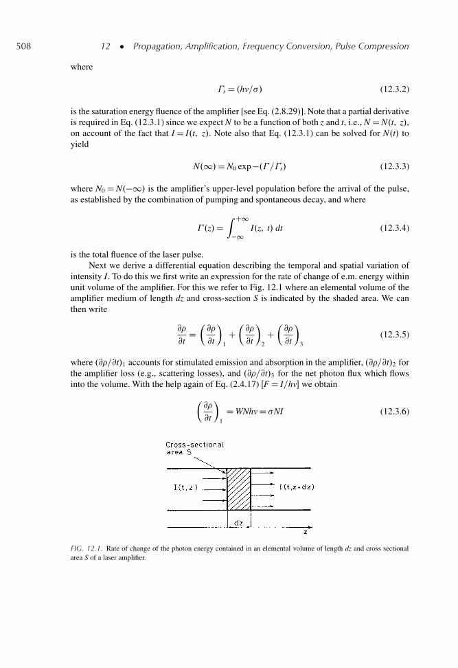
508 12 � Propagation, Amplification, Frequency Conversion, Pulse Compression
where
�s D .hv=�/ (12.3.2)
is the saturation energy fluence of the amplifier [see Eq. (2.8.29)]. Note that a partial derivativeis required in Eq. (12.3.1) since we expect N to be a function of both z and t, i.e., N D N.t, z/,on account of the fact that I D I.t, z/. Note also that Eq. (12.3.1) can be solved for N.t/ toyield
N.1/D N0 exp �.� =�s/ (12.3.3)
where N0 D N.�1/ is the amplifier’s upper-level population before the arrival of the pulse,as established by the combination of pumping and spontaneous decay, and where
� .z/DZ C1
�1I.z, t/ dt (12.3.4)
is the total fluence of the laser pulse.Next we derive a differential equation describing the temporal and spatial variation of
intensity I. To do this we first write an expression for the rate of change of e.m. energy withinunit volume of the amplifier. For this we refer to Fig. 12.1 where an elemental volume of theamplifier medium of length dz and cross-section S is indicated by the shaded area. We canthen write
@�
@tD�@�
@t
�1
C�@�
@t
�2
C�@�
@t
�3
(12.3.5)
where .@�=@t/1 accounts for stimulated emission and absorption in the amplifier, .@�=@t/2 forthe amplifier loss (e.g., scattering losses), and .@�=@t/3 for the net photon flux which flowsinto the volume. With the help again of Eq. (2.4.17) ŒF D I=hv� we obtain
�@�
@t
�1
D WNhv D �NI (12.3.6)
FIG. 12.1. Rate of change of the photon energy contained in an elemental volume of length dz and cross sectionalarea S of a laser amplifier.
12.3 � Amplitude Transformation: Laser Amplification 509
and from Eqs. (2.4.17) and (2.4.32) we obtain�@�
@t
�2
D � WaNahv D � ˛ I (12.3.7)
where Na is the density of the loss centers, while Wa is the absorption rate, and ˛ the absorp-tion coefficient associated with the loss centers. To calculate .@�=@t/3, we refer again toFig. 12.1, and note that .@�=@t/3Sdz is the rate of change of e.m. energy in this volumedue to the difference between the incoming and outgoing laser power. We can then write.@�=@t/3Sdz D SŒI.t, z/ � I.t, z C dz/�, which readily gives
�@�
@t
�3
dz D � @I
@zdz (12.3.8)
Equation (12.3.5), with the help of Eqs. (12.3.6)–(12.3.8) and with the observation that.@�=@t/D .@I=c@t/, gives
1
c
@I
@tC @I
@zD �NI � ˛I (12.3.9)
This equation, together with Eq. (12.3.1), completely describes the amplification process.Note that Eq. (12.3.9) has the usual form of a time-dependent transport equation.
Equations (12.3.1) and (12.3.9) must be solved with the appropriate boundary and initialconditions. As the initial condition we take N.0, z/D N0, where N0 is the amplifier upper-levelpopulation before the arrival of the laser pulse. The boundary condition is obviously estab-lished by the intensity I0.t/ of the light pulse injected into the amplifier, i.e., I.t, 0/D I0.t/.For negligible amplifier losses (i.e., neglecting the term �˛l), the solution to Eqs. (12.3.1)and (12.3.9) can be written as
I.z, �/D I0.�/
8<:1 � Œ1 � exp.�gz/� exp
24�
�Z�1
I0.�0/ d� 0=�s
359=;
�1
(12.3.10)
where � D t � .z=c/ and where g D �N0 is the unsaturated gain coefficient of the amplifier.From Eqs. (12.3.1) and (12.3.9), we can also obtain a differential equation for the total
fluence of the pulse, � .z/, given by Eq. (12.3.4). Thus, we first integrate both sides of
Eq. (12.3.1) with respect to time, from t D �1 to t D C1, to obtain�R C1
�1 NIdt=�s
�D N0 �
N.C1/D N0Œ1 � exp.�� =�s/�, where Eq. (12.3.3) has been used. We then integrate bothsides of Eq. (12.3.9) with respect to time, on the same time interval, and use the above
expression for�R C1
�1 NIdt=�s
�and the fact that I.C1, z/D I.�1, z/D 0. We obtain
d�
dzD g�sŒ1 � exp.�� =�s/� � ˛� (12.3.11)
Again neglecting amplifier losses, Eq. (12.3.11) gives
� .l/D�s ln
1 C
�exp
��in
�s
�� 1
�G0
�(12.3.12)
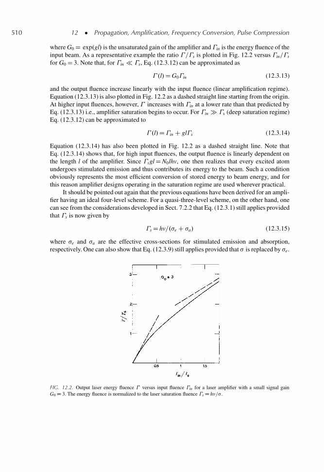
510 12 � Propagation, Amplification, Frequency Conversion, Pulse Compression
where G0 D exp.gl/ is the unsaturated gain of the amplifier and�in is the energy fluence of theinput beam. As a representative example the ratio � =�s is plotted in Fig. 12.2 versus �in=�s
for G0 D 3. Note that, for �in � �s, Eq. (12.3.12) can be approximated as
� .l/D G0�in (12.3.13)
and the output fluence increase linearly with the input fluence (linear amplification regime).Equation (12.3.13) is also plotted in Fig. 12.2 as a dashed straight line starting from the origin.At higher input fluences, however, � increases with �in at a lower rate than that predicted byEq. (12.3.13) i.e., amplifier saturation begins to occur. For �in � �s (deep saturation regime)Eq. (12.3.12) can be approximated to
� .l/D�in C gl�s (12.3.14)
Equation (12.3.14) has also been plotted in Fig. 12.2 as a dashed straight line. Note thatEq. (12.3.14) shows that, for high input fluences, the output fluence is linearly dependent onthe length l of the amplifier. Since �sgl D N0lhv, one then realizes that every excited atomundergoes stimulated emission and thus contributes its energy to the beam. Such a conditionobviously represents the most efficient conversion of stored energy to beam energy, and forthis reason amplifier designs operating in the saturation regime are used wherever practical.
It should be pointed out again that the previous equations have been derived for an ampli-fier having an ideal four-level scheme. For a quasi-three-level scheme, on the other hand, onecan see from the considerations developed in Sect. 7.2.2 that Eq. (12.3.1) still applies providedthat �s is now given by
�s D hv=.�e C �a/ (12.3.15)
where �e and �a are the effective cross-sections for stimulated emission and absorption,respectively. One can also show that Eq. (12.3.9) still applies provided that � is replaced by �e.
FIG. 12.2. Output laser energy fluence � versus input fluence �in for a laser amplifier with a small signal gainG0 D 3. The energy fluence is normalized to the laser saturation fluence �s D h�=� .
12.3 � Amplitude Transformation: Laser Amplification 511
It then follows that Eq. (12.3.12) still remain valid provided that �s is given by Eq. (12.3.15)and G0 given by G0 D exp�eN0l. Similar considerations can be made for an amplifier oper-ating on a four-level scheme when the pulse duration becomes much shorter than the lifetimeof the lower level of the transition. In this case the population driven to the lower level bystimulated emission remains in this level during the pulse and one can show that Eq. (12.3.12)still remains valid provided that � is replaced by �e, and �s is given by Eq. (12.3.15), where�a is the effective absorption cross-section of the lower level of the transition.
If amplifier losses cannot be neglected, the above picture has to be modified somewhat.In particular the output fluence � .l/ does not continue increasing with input fluence, as inFig. 12.2, but reaches a maximum and then decreases. This can be understood by notingthat, in this case, the output as a function of amplifier length tends to grow linearly due toamplification [at least for high input fluences, see Eq. (12.3.14)] and to decrease exponentiallydue to loss [on account of the term �˛� in Eq. (12.3.11)]. The competition of these two termsthen gives a maximum for the output fluence � . For ˛ � g this maximum value of the outputfluence, �m, turns out to be
�m Š g�s=˛ (12.3.16)
It should be noted, however, that, since amplifier losses are typically quite small, other phe-nomena usually limit the maximum energy fluence that can be extracted from an amplifier. Infact, the limit is usually set by the amplifier damage fluence �d (10 J=cm2 is a typical valuefor a number of solid-state media). From Eq. (12.3.14) we then get the condition
� Š gl�s<�d (12.3.17)
Another limitation to amplifier performance arises from the fact that the unsaturatedgain G0 D exp.gl/ must not be made too high, otherwise two undesirable effects can occur inthe amplifier: (1) parasitic oscillations, (2) amplified spontaneous emission (ASE). Parasiticoscillation occurs when the amplifier starts lasing by virtue of some internal feedback whichwill always be present to some degree, (e.g., due to the amplifier end faces). The phenomenonof ASE has already been discussed in Sect. 2.9.2. Both these phenomena tend to depopulatethe available inversion and hence decrease the laser gain. To minimize parasitic oscillationsone should avoid elongated amplifiers and in fact ideally use amplifiers with roughly equaldimensions in all directions. Even in this case, however, parasitic oscillations set an upperlimit .gl/max to the product of gain coefficient, g, with amplifier length, l, i.e.,
gl< .gl/max (12.3.18)
where, for typical cases, .gl/max may range between three and five. The threshold for ASEhas already been given in Sect. 2.9.2 [see Eq. (2.9.4a), for a Lorentzian line]. For an amplifierin the form of a cube (i.e., for ˝ Š 1) and for a unitary fluorescence quantum yield we getG Š 8 [i.e., gl Š 2.1] which is comparable to that established by parasitic oscillations. Forsmaller values of solid angle ˝ , which are more typical, the value of G for the onset of ASEis expected to increase [Eq. (2.9.4a)]. Hence parasitic oscillations, rather than ASE, usuallydetermine the maximum gain that can be achieved.
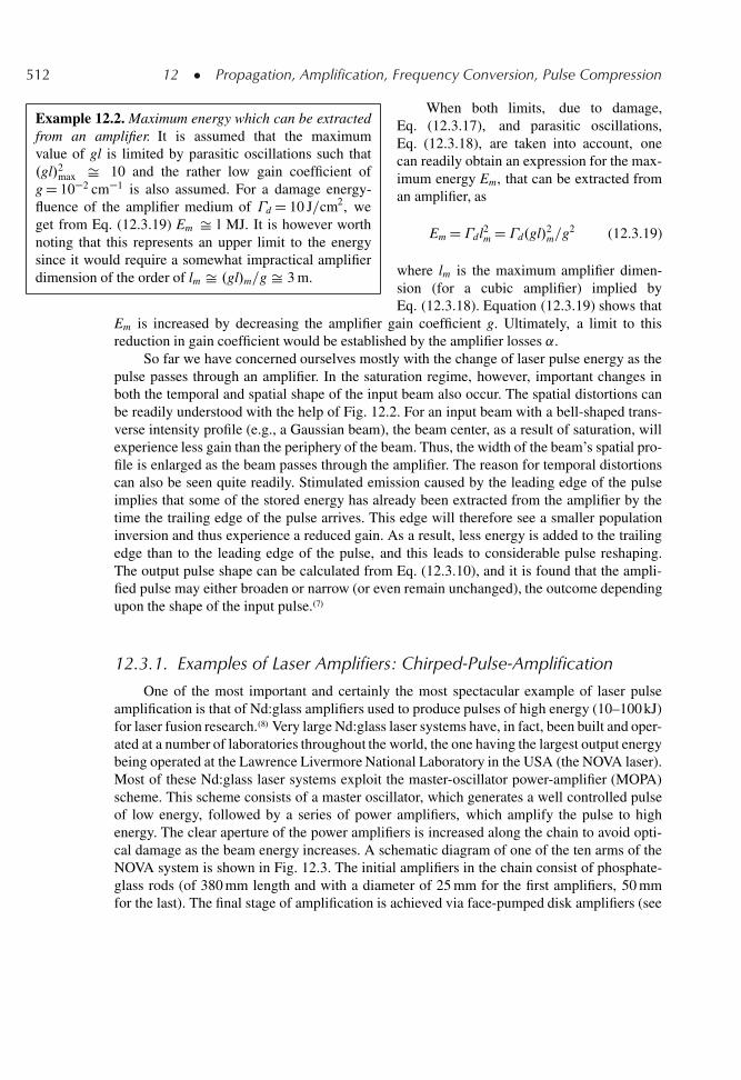
512 12 � Propagation, Amplification, Frequency Conversion, Pulse Compression
Example 12.2. Maximum energy which can be extractedfrom an amplifier. It is assumed that the maximumvalue of gl is limited by parasitic oscillations such that.gl/2max Š 10 and the rather low gain coefficient ofg D 10�2 cm�1 is also assumed. For a damage energy-fluence of the amplifier medium of �d D 10 J=cm2, weget from Eq. (12.3.19) Em Š l MJ. It is however worthnoting that this represents an upper limit to the energysince it would require a somewhat impractical amplifierdimension of the order of lm Š .gl/m=g Š 3 m.
When both limits, due to damage,Eq. (12.3.17), and parasitic oscillations,Eq. (12.3.18), are taken into account, onecan readily obtain an expression for the max-imum energy Em, that can be extracted froman amplifier, as
Em D�dl2m D�d.gl/2m=g2 (12.3.19)
where lm is the maximum amplifier dimen-sion (for a cubic amplifier) implied byEq. (12.3.18). Equation (12.3.19) shows that
Em is increased by decreasing the amplifier gain coefficient g. Ultimately, a limit to thisreduction in gain coefficient would be established by the amplifier losses ˛.
So far we have concerned ourselves mostly with the change of laser pulse energy as thepulse passes through an amplifier. In the saturation regime, however, important changes inboth the temporal and spatial shape of the input beam also occur. The spatial distortions canbe readily understood with the help of Fig. 12.2. For an input beam with a bell-shaped trans-verse intensity profile (e.g., a Gaussian beam), the beam center, as a result of saturation, willexperience less gain than the periphery of the beam. Thus, the width of the beam’s spatial pro-file is enlarged as the beam passes through the amplifier. The reason for temporal distortionscan also be seen quite readily. Stimulated emission caused by the leading edge of the pulseimplies that some of the stored energy has already been extracted from the amplifier by thetime the trailing edge of the pulse arrives. This edge will therefore see a smaller populationinversion and thus experience a reduced gain. As a result, less energy is added to the trailingedge than to the leading edge of the pulse, and this leads to considerable pulse reshaping.The output pulse shape can be calculated from Eq. (12.3.10), and it is found that the ampli-fied pulse may either broaden or narrow (or even remain unchanged), the outcome dependingupon the shape of the input pulse..7/
12.3.1. Examples of Laser Amplifiers: Chirped-Pulse-Amplification
One of the most important and certainly the most spectacular example of laser pulseamplification is that of Nd:glass amplifiers used to produce pulses of high energy (10–100 kJ)for laser fusion research..8/ Very large Nd:glass laser systems have, in fact, been built and oper-ated at a number of laboratories throughout the world, the one having the largest output energybeing operated at the Lawrence Livermore National Laboratory in the USA (the NOVA laser).Most of these Nd:glass laser systems exploit the master-oscillator power-amplifier (MOPA)scheme. This scheme consists of a master oscillator, which generates a well controlled pulseof low energy, followed by a series of power amplifiers, which amplify the pulse to highenergy. The clear aperture of the power amplifiers is increased along the chain to avoid opti-cal damage as the beam energy increases. A schematic diagram of one of the ten arms of theNOVA system is shown in Fig. 12.3. The initial amplifiers in the chain consist of phosphate-glass rods (of 380 mm length and with a diameter of 25 mm for the first amplifiers, 50 mmfor the last). The final stage of amplification is achieved via face-pumped disk amplifiers (see
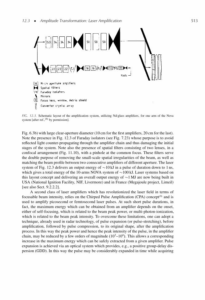
12.3 � Amplitude Transformation: Laser Amplification 513
FIG. 12.3. Schematic layout of the amplification system, utilizing Nd:glass amplifiers, for one arm of the Novasystem [after ref.,.8/ by permission].
Fig. 6.3b) with large clear-aperture diameter (10 cm for the first amplifiers, 20 cm for the last).Note the presence in Fig. 12.3 of Faraday isolators (see Fig. 7.23) whose purpose is to avoidreflected light counter-propagating through the amplifier chain and thus damaging the initialstages of the system. Note also the presence of spatial filters consisting of two lenses, in aconfocal arrangement (Fig. 11.10), with a pinhole at the common focus. These filters servethe double purpose of removing the small-scale spatial irregularities of the beam, as well asmatching the beam profile between two consecutive amplifiers of different aperture. The lasersystem of Fig. 12.3 delivers an output energy of �10 kJ in a pulse of duration down to 1 ns,which gives a total energy of the 10-arms NOVA system of �100 kJ. Laser systems based onthis layout concept and delivering an overall output energy of �1 MJ are now being built inUSA (National Ignition Facility, NIF, Livermore) and in France (Megajoule project, Limeil)[see also Sect. 9.2.2.2].
A second class of laser amplifiers which has revolutionized the laser field in terms offocusable beam intensity, relies on the Chirped Pulse Amplification (CPA) concept.9/ and isused to amplify picosecond or femtosecond laser pulses. At such short pulse durations, infact, the maximum energy which can be obtained from an amplifier depends on the onset,either of self-focusing, which is related to the beam peak power, or multi-photon-ionization,which is related to the beam peak intensity. To overcome these limitations, one can adopt atechnique, already used in radar technology, of pulse expansion (or pulse-stretching), beforeamplification, followed by pulse compression, to its original shape, after the amplificationprocess. In this way the peak power and hence the peak intensity of the pulse, in the amplifierchain, may be reduced by a few orders of magnitude .103–104/. This allows a correspondingincrease in the maximum energy which can be safely extracted from a given amplifier. Pulseexpansion is achieved via an optical system which provides, e.g., a positive group-delay dis-persion (GDD). In this way the pulse may be considerably expanded in time while acquiring
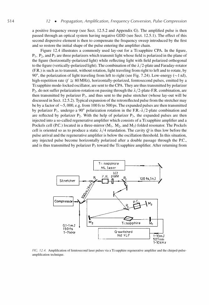
514 12 � Propagation, Amplification, Frequency Conversion, Pulse Compression
a positive frequency sweep (see Sect. 12.5.2 and Appendix G). The amplified pulse is thenpassed through an optical system having negative GDD (see Sect. 12.5.1). The effect of thissecond dispersive element is then to compensate the frequency sweep introduced by the firstand so restore the initial shape of the pulse entering the amplifier chain.
Figure 12.4 illustrates a commonly used lay-out for a Ti:sapphire CPA. In the figure,P1, P2, and P3 are three polarizers which transmit light whose field is polarized in the plane ofthe figure (horizontally-polarized light) while reflecting light with field polarized orthogonalto the figure (vertically-polarized light). The combination of the �=2-plate and Faraday-rotator(F.R.) is such as to transmit, without rotation, light traveling from right to left and to rotate, by90ı, the polarization of light traveling from left to right (see Fig. 7.24). Low-energy .�1 nJ/,high-repetition rate .f Š 80 MHz/, horizontally-polarized, femtosecond pulses, emitted by aTi:sapphire mode-locked oscillator, are sent to the CPA. They are thus transmitted by polarizerP2, do not suffer polarization-rotation on passing through the �=2-plate-F.R. combination, arethen transmitted by polarizer P1, and thus sent to the pulse stretcher (whose lay-out will bediscussed in Sect. 12.5.2). Typical expansion of the retroreflected pulse from the stretcher maybe by a factor of �5, 000, e.g. from 100 fs to 500 ps. The expanded pulses are then transmittedby polarizer P1, undergo a 90ı polarization rotation in the F.R.-�=2-plate combination andare reflected by polarizer P2. With the help of polarizer P3, the expanded pulses are theninjected into a so-called regenerative amplifier which consists of a Ti:sapphire amplifier and aPockels cell (P.C.) located in a three-mirror (M1, M2, and M3) folded resonator. The Pockelscell is oriented so as to produce a static �=4 retardation. The cavity Q is thus low before thepulse arrival and the regenerative amplifier is below the oscillation threshold. In this situation,any injected pulse become horizontally polarized after a double passage through the P.C.,and is thus transmitted by polarizer P3 toward the Ti:sapphire amplifier. After returning from
FIG. 12.4. Amplification of femtosecond laser pulses via a Ti:sapphire regenerative amplifier and the chirped-pulse-amplification technique.
12.3 � Amplitude Transformation: Laser Amplification 515
the amplifier, the pulse is transmitted by polarizer P3, and, after again double-passing theP.C., becomes vertically polarized and thus reflected out of the cavity by polarizer P3. So,in this double transit through the regenerative amplifier, very little amplification is obtainedfor the output pulse. If however, while the pulse is between the polarizer and mirror M1, a�=4-voltage is applied to the P.C., the cell becomes equivalent to a �=2-plate, and the pulsedoes not change its polarization state after each double passage through the cell. Therefore,the pulse gets trapped in the regenerative amplifier and, on each pass through the amplifyingmedium, it is amplified. After a suitable number of round-trips in the cavity (typically 15–20),the pulse energy reaches its maximum value and is then extracted from the cavity by applyingan additional �=4 voltage to the P.C.. In this case, in fact, after a double pass through the cell,the pulse becomes vertically polarized and is reflected by polarizer P3 back in the directionof the incoming pulses. This, high-energy, vertically-polarized pulse is reflected by polarizerP2, does not suffer polarization-rotation on passing through the �/2-plate-F.R. combination,and is reflected by polarizer P1 toward the pulse compressor (whose lay-out will be discussedin Sect. 12.5.1). The retroreflected beam from the compressor then consists of a train of highenergy pulses, each with a duration approximately equal to that of the original pulses emittedby the oscillator, and with a repetition rate equal to that at which the Ti:sapphire amplifier ispumped (1–10 kHz, usually by the second-harmonic green-beam of a repetitively Q-switchedNd:YLF laser).
Systems of this type, exploiting the CPA technique, have allowed the development oflasers with ultra-high peak-power..10/ For instance, using Ti:sapphire active media, table-topCPA systems with peak power of �20 TW have already been demonstrated while systemswith peak powers approaching 100 TW (e.g., 2 J in a 20 fs pulse) are under construc-tion. The largest peak power, so far achieved by exploiting the CPA technique, is actually�1.25 PW .1 PW D 1015 W/,.11/ obtained using a chain of amplifiers taken from one arm ofthe NOVA laser (so as to obtain an amplified pulse with �580 J energy and �460 fs dura-tion). The peak intensity obtained by focusing these ultra-high-power pulses is extremely high.1019–1020 W=cm2/, representing an increase of four to five orders of magnitude compared tothat available before introducing the CPA technique. When these ultra-high intensity beamsinteract with a solid target or with a gas, a highly ionized plasma is obtained and a completelynew class of nonlinear optical phenomena is produced. Applications of these high intensi-ties cover a broad area of science and technology including ultrafast x-ray and high-energyelectron sources, as well as novel fusion concepts and plasma astrophysics..12/
A third class of amplifier, widely used in optical fiber communications, is represented bythe Er-doped optical-fiber amplifier (EDFA)..13/ This amplifier is diode-pumped either in the980 nm or 1480 nm pump bands of the ErC ion [see Fig. 9.4] and is used to amplify pulses atwavelengths corresponding to the so-called third transmission window of silica optical fibers.� Š 1550 nm/. Since, usually, the pulse repetition rate of a communication system is veryhigh .� GHz/ and the upper-state lifetime of ErC is very long (�10 ms, see Table 9.4) thesaturation behavior of the ErC population is a cumulative result of many laser pulses, i.e.,determined by the average beam intensity. The rate-equation treatment of this type of ampli-fication can then be made in terms of average beam intensity and, in principle, is very simple.Complications however arise from several factors, namely: (1) The ErC system works on analmost pure three-level scheme (see Sect. 9.2.4) and therefore, the effective cross-sections ofstimulated-emission and absorption, both covering a large spectral bandwidth, must be takeninto account. (2) Transverse variation, within the fiber, of both the ErC population profile and
516 12 � Propagation, Amplification, Frequency Conversion, Pulse Compression
the intensity profile of the propagating mode, must be taken into account. (3) Account mustalso be taken of the simultaneous presence of bidirectional noise arising from amplified spon-taneous emission (ASE). We therefore make no attempt to cover this subject in any detail,limiting ourselves to pointing out that a vast literature exists,.14/ that very high small-signalgain (up to �50 dB), relatively large saturated average output powers .�100 mW/, and lownoise are achieved via these amplifiers. Thus, Erbium-doped fiber amplifiers must be con-sidered a major break-through in the field of optical fiber communications, with applicationsregarding both long-haul systems as well as distribution networks.
12.4. FREQUENCY CONVERSION: SECOND-HARMONICGENERATION AND PARAMETRIC OSCILLATION.1,15/
In classical linear optics one assumes that the induced dielectric polarization of a mediumis linearly related to the applied electric field, i.e.,
P D "0�E (12.4.1)
where � is the dielectric susceptibility. With the high electric fields involved in laser beamsthe above linear relation is no longer a good approximation, and further terms in which P isrelated to higher-order powers of E must also be considered. This nonlinear response can leadto an exchange of energy between e.m. waves at different frequencies.
In this section we will consider some of the effects produced by a nonlinear polarizationterm that is proportional to the square of the electric field. The two effects that we will considerare: (1) Second-harmonic generation (SHG), in which a laser beam at frequency ! is partiallyconverted, in the nonlinear material, to a coherent beam at frequency 2! [as first shown byFranken et al..16/]. (2) Optical parameter oscillation (OPO), in which a laser beam at frequency!3 causes the simultaneous generation, in the nonlinear material, of two coherent beams atfrequency !1 and !2 such that !1 C!2 D!3 [as first shown by Giordmaine and Miller.17/].With the high electric fields available in laser beams the conversion efficiency of both theseprocesses can be very high (approaching 100% in SHG). Therefore, these techniques areincreasingly used to generate new coherent waves at different frequencies from that of theincoming wave.
12.4.1. Physical Picture
We will first introduce some physical concepts using the simplifying assumption that theinduced nonlinear polarization PNL is related to the electric field E of the e.m. wave by a scalarequation, i.e.,
PNL D 2ε0dE2 (12.4.2)
where d is a coefficient whose dimension is the inverse of an electric field.� The physical ori-gin of Eq. (12.4.2) resides in the nonlinear deformation of the outer, loosely bound, electrons
� We use 2ε0 dE2 rather than dE2 (as often used in other textbooks) to make d conform to increasingly acceptedpractice.
12.4 � Frequency Conversion: Second-Harmonic Generation 517
of an atom or atomic system when subjected to high electric fields. This is analogous to abreakdown of Hooke’s law for an extended spring, resulting in the restoring force no longerbeing linearly dependent on the displacement from equilibrium. A comparison of Eqs. (12.4.2)and (12.4.1) shows that the nonlinear polarization term becomes comparable to the linear onefor an electric field E Š �=d. Since � Š 1, we see that .1=d/ represents the field strengthfor which the linear and nonlinear terms become comparable. At this field strength, a sizablenonlinear deformation of the outer electrons must occur and .1=d/ is then expected to be ofthe order of the electric field that an electronic charge produces at a distance correspondingto a typical atomic dimension a, i.e., .1=d/ Š e=4 ε0a2 [thus .1=d/ Š 1011 V=m for a Š0.1 nm]. We note that d must be zero for a centrosymmetric material, such as a centrosym-metric crystal or the usual liquids and gases. For symmetry reasons, in fact, if we reverse thesign of E, the sign of the total polarization Pt D P C PNL must also reverse. Since, however,PNL / dE2, this can only occur if d D 0. From now on we will therefore confine ourselves toa consideration of non-centrosymmetric materials. We will see that the simple Eq. (12.4.2) isthen able to account for both SHG and OPO.
12.4.1.1. Second-Harmonic Generation
We consider a monochromatic plane wave of frequency! propagating along some direc-tion, denoted as the z-direction, within a nonlinear crystal, the origin of the z-axis being takenat the entrance face of the crystal. For a plane wave of uniform intensity we can write thefollowing expression for the electric field E!.z, t/ of the wave
E!.z, t/D .1=2/ fE.z, !/ expŒj.! t � k!z/�C c.c.g (12.4.3)
In the above expression c.c. means the complex conjugate of the other term appearing in thebrackets and
k! D !
c!
D n!!
c(12.4.4)
where c! is the phase velocity, in the crystal, of a wave of frequency !, n! is the refractiveindex at this frequency, and c is the velocity of light in vacuum. Substitution of Eq. (12.4.3)into Eq. (12.4.2) shows that PNL contains a term� oscillating at frequency 2!, namely,
PNL2! D ."0d=2/
˚E2.z, !/ expŒj.2! t � 2k!z/�C c.c.
�(12.4.5)
Equation (12.4.5) describes a polarization wave oscillating at frequency 2! and witha propagation constant 2k! . This wave is then expected to radiate at frequency 2!, i.e., togenerate an e.m. wave at the second harmonic (SH) frequency 2!. The analytical treatment,given later, involves in fact substitution of this polarization in the wave equation for the e.m.field. The radiated SH field can be written in the form
E2!.z, t/D .1=2/ fE.z, 2!/ expŒj.2! t � k2!z/�C c.c.g (12.4.6)
� The quantity PNL also contains a term at frequency !D 0 which leads to development of a dc voltage across thecrystal (optical rectification).
518 12 � Propagation, Amplification, Frequency Conversion, Pulse Compression
where
k2! D 2!
c2!
D 2n2!!
c(12.4.7)
is the propagation constant of a wave at frequency 2!. The physical origin of SHG can thus betraced back to the fact that, as a result of the nonlinear relation Eq. (12.4.2), the e.m. wave atthe fundamental frequency ! will beat with itself to produce a polarization at 2!. A compari-son of Eq. (12.4.5) with Eq. (12.4.6) reveals a very important condition that must be satisfiedif this process is to occur efficiently, viz., that the phase velocity of the polarization wave.�P D 2!=2k!/ be equal to that of the generated e.m. wave .�E D 2!=k2!/. This conditioncan thus be written as
k2! D 2k! (12.4.8)
In fact, if this condition is not satisfied, the phase of the polarization wave at coordinatez D l into the crystal, 2k!l, will be different from that, k2! l, of the wave generated at z D 0which has subsequently propagated to z D l. The difference in phase, .2k! �k2!/l, would thenincrease with distance l and the generated wave, being driven by a polarization which does nothave the appropriate phase, will then not grow cumulatively with distance l. Equation (12.4.8)is therefore referred to as the phase-matching condition. Note that, according to Eqs. (12.4.4)and (12.4.7), equation (12.4.8) implies that
n2! D n! (12.4.9)
Now, if the polarization directions of E! and PNL (and hence of E2!/ were indeed thesame [as implied by Eq. (12.4.2)] condition Eq. (12.4.9) could not be satisfied owing to thedispersion .n D n2! � n!/ of the crystal. This would then set a severe limit to the crystallength lc over which PNL can give contributions which keep adding cumulatively to form thesecond harmonic wave. This length lc (the coherence length) must in fact correspond to thedistance over which the polarization wave and the SH wave get out of phase with each otherby an amount . This means that k2!lc �2k!lc D , from which, with the help of Eqs. (12.4.4)and (12.4.7), one gets
lc D �
4 n(12.4.10)
where �D 2 c=! is the wavelength in vacuum of the fundamental wave. Taking, as an exam-ple, � Š 1�m and n D 10�2, we get lc D 25�m. Note that, at this distance into the crystal,the polarization wave becomes 180ı out of phase compared to the SH wave and the latterbegins to decrease with increased distance rather than continuing to grow. Since, as seen inthe previous example, lc is usually very small, only a very small fraction of the incident powercan then be transformed into the second harmonic wave.
At this point it is worth pointing out another useful way of visualizing the SHG process,in terms of photons rather than fields. First we write the relation between the frequency of thefundamental (!) and second-harmonic .!SH/ wave, viz.,
!SH D 2! (12.4.11)
12.4 � Frequency Conversion: Second-Harmonic Generation 519
If we now multiply both sides of Eqs. (12.4.11) and (12.4.8) by „, we get
„!SH D 2„! (12.4.12a)
„k2! D 2„k! (12.4.12b)
respectively. For energy to be conserved in the SHG process, we must have dI2!=dz D�dI!=dz, where I2! and I! are the intensities of the waves at the two frequencies. Withthe help of Eq. (12.4.12a) we get dF2!=dz D �.1=2/dF!=dz, where F2! and F! are the pho-ton fluxes of the two waves. From this equation we can then say that, whenever, in the SHGprocess, one photon at frequency 2! is produced, correspondingly two photons at frequency! disappear. Thus the relation Eq. (12.4.12a) can be regarded as a statement of conservationof photon energy. Remembering that „k is the photon momentum, Eq. (12.4.12b) is then seento correspond to the requirement that photon momentum is also conserved in the process.
We now reconsider the phase-matching condition Eq. (12.4.9) to see how it can be sat-isfied in a suitable, optically anisotropic, crystal..18,19/ To understand this we will first needto make a small digression to explain the propagation behavior of waves in an anisotropiccrystal, and also to show how the simple nonlinear relation Eq. (12.4.2) should be generalizedfor anisotropic media.
In an anisotropic crystal it can be shown that, for a given direction of propagation, thereare two linearly polarized plane waves that can propagate with different phase velocities. Cor-responding to these two different polarizations one can then associate two different refractiveindices, the difference of refractive index being referred to as the crystal’s birefringence. Thisbehavior is usually described in terms of the so-called index ellipsoid which, for a uniaxialcrystal, is an ellipsoid of revolution around the optic axis (the z axis of Fig. 12.5). Given thisellipsoid, the two allowed directions of linear polarization and their corresponding refractiveindices are found as follows: Through the center of the ellipsoid one draws a line in the direc-tion of beam propagation (line OP of Fig. 12.5) and a plane perpendicular to this line. Theintersection of this plane with the ellipsoid is an ellipse. The direction of the two axes of theellipse then give the two polarization directions and the length of each semiaxis gives therefractive index corresponding to that polarization. One of these directions is necessarily per-pendicular to the optic axis and the wave having this polarization is referred to as the ordinarywave. Its refractive index, no, can be seen from the figure to be independent of the directionof propagation. The wave with the other direction of polarization is referred to as the extraor-dinary wave and the corresponding index, ne./, depends of the angle and ranges in valuefrom that of the ordinary wave n0 (when OP is parallel to z) to the value ne, referred to as theextraordinary index, which occurs when OP is perpendicular to z. Note now that one defines apositive uniaxial crystal as corresponding to the case ne> no while a negative uniaxial crystalcorresponds to the case ne< no. An equivalent way to describe wave propagation is throughthe so-called normal (index) surfaces for the ordinary and extraordinary waves (Fig. 12.6). Inthis case, for a given direction of propagation OP and, for either ordinary or extraordinarywaves, the length of the segment between the origin O and the point of interception of the rayOP with the surface gives the refractive index of that wave. The normal surface for the ordi-nary wave is thus a sphere, while the normal surface for the extraordinary wave is an ellipsoidof revolution around the z axis. In Fig. 12.6 the intersections of these two normal surfaceswith the y-z plane are indicated for the case of a positive uniaxial crystal.
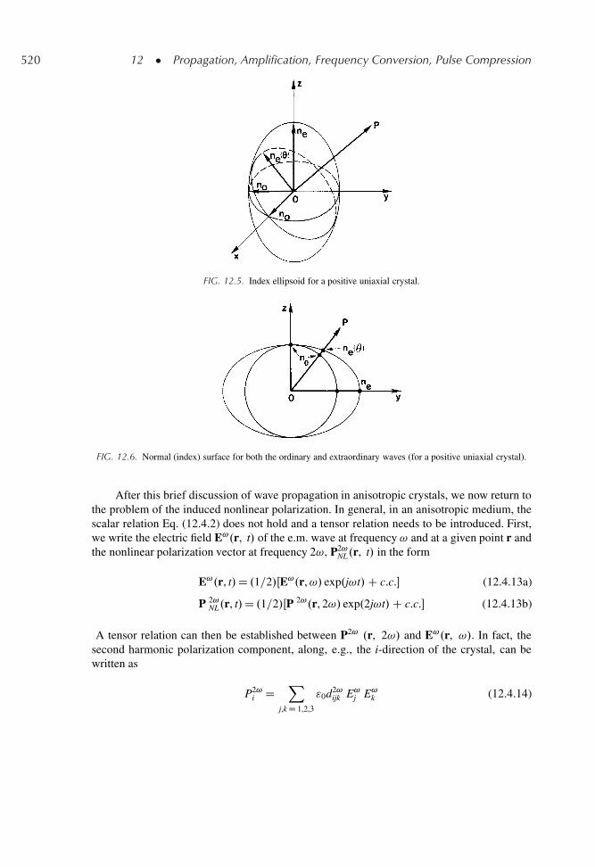
520 12 � Propagation, Amplification, Frequency Conversion, Pulse Compression
FIG. 12.5. Index ellipsoid for a positive uniaxial crystal.
FIG. 12.6. Normal (index) surface for both the ordinary and extraordinary waves (for a positive uniaxial crystal).
After this brief discussion of wave propagation in anisotropic crystals, we now return tothe problem of the induced nonlinear polarization. In general, in an anisotropic medium, thescalar relation Eq. (12.4.2) does not hold and a tensor relation needs to be introduced. First,we write the electric field E!.r, t/ of the e.m. wave at frequency ! and at a given point r andthe nonlinear polarization vector at frequency 2!, P2!
NL.r, t/ in the form
E!.r, t/D .1=2/ŒE!.r,!/ exp.j!t/C c.c.� (12.4.13a)
P 2!NL.r, t/D .1=2/ŒP 2!.r, 2!/ exp.2j!t/C c.c.� (12.4.13b)
A tensor relation can then be established between P2! .r, 2!/ and E!.r, !/. In fact, thesecond harmonic polarization component, along, e.g., the i-direction of the crystal, can bewritten as
P2!i D
Xj,k D 1,2,3
"0d2!ijk E!
j E!k (12.4.14)
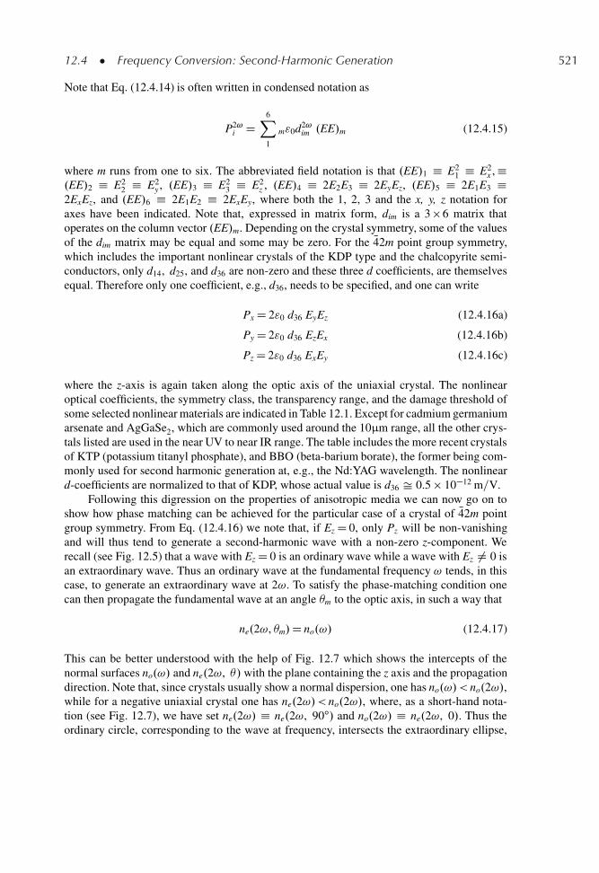
12.4 � Frequency Conversion: Second-Harmonic Generation 521
Note that Eq. (12.4.14) is often written in condensed notation as
P2!i D
6X1
m"0d2!im .EE/m (12.4.15)
where m runs from one to six. The abbreviated field notation is that .EE/1 � E21 � E2
x , �.EE/2 � E2
2 � E2y , .EE/3 � E2
3 � E2z , .EE/4 � 2E2E3 � 2EyEz, .EE/5 � 2E1E3 �
2ExEz, and .EE/6 � 2E1E2 � 2ExEy, where both the 1, 2, 3 and the x, y, z notation foraxes have been indicated. Note that, expressed in matrix form, dim is a 3 � 6 matrix thatoperates on the column vector .EE/m. Depending on the crystal symmetry, some of the valuesof the dim matrix may be equal and some may be zero. For the N42m point group symmetry,which includes the important nonlinear crystals of the KDP type and the chalcopyrite semi-conductors, only d14, d25, and d36 are non-zero and these three d coefficients, are themselvesequal. Therefore only one coefficient, e.g., d36, needs to be specified, and one can write
Px D 2"0 d36 EyEz (12.4.16a)
Py D 2"0 d36 EzEx (12.4.16b)
Pz D 2"0 d36 ExEy (12.4.16c)
where the z-axis is again taken along the optic axis of the uniaxial crystal. The nonlinearoptical coefficients, the symmetry class, the transparency range, and the damage threshold ofsome selected nonlinear materials are indicated in Table 12.1. Except for cadmium germaniumarsenate and AgGaSe2, which are commonly used around the 10μm range, all the other crys-tals listed are used in the near UV to near IR range. The table includes the more recent crystalsof KTP (potassium titanyl phosphate), and BBO (beta-barium borate), the former being com-monly used for second harmonic generation at, e.g., the Nd:YAG wavelength. The nonlineard-coefficients are normalized to that of KDP, whose actual value is d36 Š 0.5 � 10�12 m=V.
Following this digression on the properties of anisotropic media we can now go on toshow how phase matching can be achieved for the particular case of a crystal of N42m pointgroup symmetry. From Eq. (12.4.16) we note that, if Ez D 0, only Pz will be non-vanishingand will thus tend to generate a second-harmonic wave with a non-zero z-component. Werecall (see Fig. 12.5) that a wave with Ez D 0 is an ordinary wave while a wave with Ez ¤ 0 isan extraordinary wave. Thus an ordinary wave at the fundamental frequency ! tends, in thiscase, to generate an extraordinary wave at 2!. To satisfy the phase-matching condition onecan then propagate the fundamental wave at an angle m to the optic axis, in such a way that
ne.2!, m/D no.!/ (12.4.17)
This can be better understood with the help of Fig. 12.7 which shows the intercepts of thenormal surfaces no.!/ and ne.2!, / with the plane containing the z axis and the propagationdirection. Note that, since crystals usually show a normal dispersion, one has no.!/< no.2!/,while for a negative uniaxial crystal one has ne.2!/< no.2!/, where, as a short-hand nota-tion (see Fig. 12.7), we have set ne.2!/ � ne.2!, 90ı/ and no.2!/ � ne.2!, 0/. Thus theordinary circle, corresponding to the wave at frequency, intersects the extraordinary ellipse,
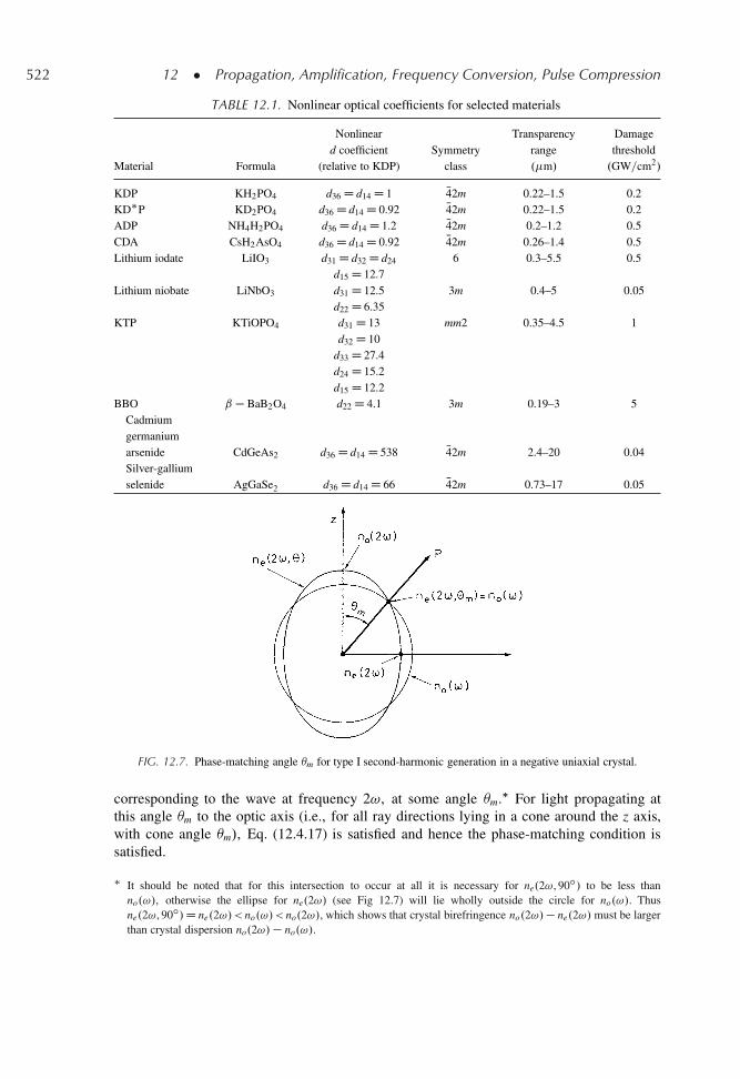
522 12 � Propagation, Amplification, Frequency Conversion, Pulse Compression
TABLE 12.1. Nonlinear optical coefficients for selected materials
Nonlinear Transparency Damaged coefficient Symmetry range threshold
Material Formula (relative to KDP) class .�m/ .GW=cm2/
KDP KH2PO4 d36 D d14 D 1 N42m 0.22–1.5 0.2KD�P KD2PO4 d36 D d14 D 0.92 N42m 0.22–1.5 0.2ADP NH4H2PO4 d36 D d14 D 1.2 N42m 0.2–1.2 0.5CDA CsH2AsO4 d36 D d14 D 0.92 N42m 0.26–1.4 0.5Lithium iodate LiIO3 d31 D d32 D d24 6 0.3–5.5 0.5
d15 D 12.7Lithium niobate LiNbO3 d31 D 12.5 3m 0.4–5 0.05
d22 D 6.35KTP KTiOPO4 d31 D 13 mm2 0.35–4.5 1
d32 D 10d33 D 27.4d24 D 15.2d15 D 12.2
BBO ˇ � BaB2O4 d22 D 4.1 3m 0.19–3 5Cadmiumgermaniumarsenide CdGeAs2 d36 D d14 D 538 N42m 2.4–20 0.04Silver-galliumselenide AgGaSe2 d36 D d14 D 66 N42m 0.73–17 0.05
FIG. 12.7. Phase-matching angle m for type I second-harmonic generation in a negative uniaxial crystal.
corresponding to the wave at frequency 2!, at some angle m.� For light propagating atthis angle m to the optic axis (i.e., for all ray directions lying in a cone around the z axis,with cone angle m/, Eq. (12.4.17) is satisfied and hence the phase-matching condition issatisfied.
� It should be noted that for this intersection to occur at all it is necessary for ne.2!, 90ı/ to be less thanno.!/, otherwise the ellipse for ne.2!/ (see Fig 12.7) will lie wholly outside the circle for no.!/. Thusne.2!, 90ı/D ne.2!/< no.!/< no.2!/, which shows that crystal birefringence no.2!/� ne.2!/must be largerthan crystal dispersion no.2!/� no.!/.
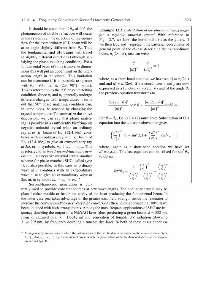
12.4 � Frequency Conversion: Second-Harmonic Generation 523
Example 12.3. Calculation of the phase-matching anglefor a negative uniaxial crystal. With reference toFig. 12.7, we label the horizontal-axis as the y-axis. Ifwe then let z and y represent the cartesian coordinates ofgeneral point of the ellipse describing the extraordinaryindex, ne.2!, /, one can write
z2
no
2
�2 C y2
ne
2
�2 D 1
where, as a short-hand notation, we have set no2 D no.2!/
and and ne2 D ne.2!/. If the coordinates z and y are now
expressed as a function of ne.2!, / and of the angle ,the previous equation transforms to
Œne.2!, /�2no
2
�2 cos2 C Œne.2!, /�2ne
2
�2 sin2 D 1
For D m, Eq. (12.4.17) must hold. Substitution of thisequation into the equation above then gives
�no
1
no2
�2
.1 � sin2m/C�
no1
ne2
�2
sin2m D 1
where, again as a short-hand notation we have setno
1 D no.!/. This last equation can be solved for sin2 m
to obtain
sin2m D1 �
�no
1no
2
�2
�no
1ne
2
�2 ��
no1
no2
�2 D�
no2
no1
�2 � 1�
no2
ne2
�2 � 1
It should be noted that, if m ¤ 90ı, thephenomenon of double refraction will occurin the crystal, i.e., the direction of the energyflow for the extraordinary (SH) beam will beat an angle slightly different from m. Thusthe fundamental and SH beams will travelin slightly different directions (although sat-isfying the phase-matching condition). For afundamental beam of finite transverse dimen-sions this will put an upper limit on the inter-action length in the crystal. This limitationcan be overcome if it is possible to operatewith m D 90ı, i.e., ne .2!, 90ı/D no.!/.This is referred to as the 90ı phase matchingcondition. Since ne and no generally undergodifferent changes with temperature, it turnsout that 90ı phase matching condition can,in some cases, be reached by changing thecrystal temperature. To summarize the abovediscussion, we can say that phase match-ing is possible in a (sufficiently birefringent)negative uniaxial crystal when an ordinaryray at ! [Ex beam of Eq. (12.4.16c)] com-bines with an ordinary ray at ! [Ey beam ofEq. (12.4.16c)] to give an extraordinary rayat 2!, or, in symbols, o! C o! ! e2! . Thisis referred to as type I second-harmonic gen-eration. In a negative uniaxial crystal anotherscheme for phase-matched SHG, called typeII, is also possible. In this case an ordinarywave at ! combines with an extraordinarywave ! at to give an extraordinary wave at2!, or, in symbols, o! C e! ! e2! .�
Second-harmonic generation is cur-rently used to provide coherent sources at new wavelengths. The nonlinear crystal may beplaced either outside or inside the cavity of the laser producing the fundamental beam. Inthe latter case one takes advantage of the greater e.m. field strength inside the resonator toincrease the conversion efficiency. Very high conversion efficiencies (approaching 100%) havebeen obtained with both arrangements. Among the most frequent applications of SHG are fre-quency doubling the output of a Nd:YAG laser (thus producing a green beam, �D 532 nm,from an infrared one, �D 1.064�m) and generation of tunable UV radiation (down to� Š 205 nm) by frequency doubling a tunable dye laser. In both of these cases either cw
� More generally, interactions in which the polarizations of the two fundamental waves are the same are termed typeI (e.g., also e! C e! ! o2! ), and interactions in which the polarization of the fundamental waves are orthogonalare termed type II.
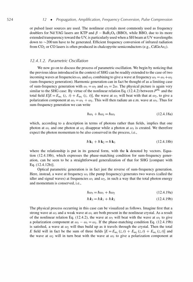
524 12 � Propagation, Amplification, Frequency Conversion, Pulse Compression
or pulsed laser sources are used. The nonlinear crystals most commonly used as frequencydoublers for Nd:YAG lasers are KTP and ˇ � BaB2O4 (BBO), while BBO, due to its moreextended transparency toward the UV, is particularly used when a SH beam at UV wavelengthsdown to �200 nm have to be generated. Efficient frequency conversion of infrared radiationfrom CO2 or CO lasers is often produced in chalcopyrite semiconductors (e.g., CdGeAs2).
12.4.1.2. Parametric Oscillation
We now go on to discuss the process of parametric oscillation. We begin by noticing thatthe previous ideas introduced in the context of SHG can be readily extended to the case of twoincoming waves at frequencies!1 and!2 combining to give a wave at frequency!3 D!1C!2
(sum-frequency generation). Harmonic generation can in fact be thought of as a limiting caseof sum-frequency generation with !1 D!2 and !3 D 2!. The physical picture is again verysimilar to the SHG case: By virtue of the nonlinear relation Eq. (12.4.2) between PNL and thetotal field EŒE D E!1 .z, t/ C E!2 .z, t/�, the wave at !1 will beat with that at !2, to give apolarization component at !3 D!1 C !2. This will then radiate an e.m. wave at !3. Thus forsum-frequency generation we can write
„!1 C „!2 D „!3 (12.4.18a)
which, according to a description in terms of photons rather than fields, implies that onephoton at !1 and one photon at !2 disappear while a photon at !3 is created. We thereforeexpect the photon momentum to be also conserved in the process, i.e.,
„ k1 C „ k2 D „ k3 (12.4.18b)
where the relationship is put in its general form, with the k denoted by vectors. Equa-tion (12.4.18b), which expresses the phase-matching condition for sum-frequency gener-ation, can be seen to be a straightforward generalization of that for SHG [compare withEq. (12.4.12b)].
Optical parametric generation is in fact just the reverse of sum-frequency generation.Here, instead, a wave at frequency !3 (the pump frequency) generates two waves (called theidler and signal waves) at frequencies !1 and !2, in such a way that the total photon energyand momentum is conserved, i.e.,
„!3 D „!1 C „!2 (12.4.19a)
„ k3 D „ k1 C „ k2 (12.4.19b)
The physical process occurring in this case can be visualized as follows. Imagine first that astrong wave at !3 and a weak wave at !1 are both present in the nonlinear crystal. As a resultof the nonlinear relation Eq. (12.4.2), the wave at !3 will beat with the wave at !1 to givea polarization component at !3 � !1 D!2. If the phase-matching condition Eq. (12.4.19b)is satisfied, a wave at !2 will thus build up as it travels through the crystal. Then the totalE field will in fact be the sum of three fields ŒE D E!1 .z, t/ C E!2 .z, t/ C E!3 .z, t/� andthe wave at !2 will in turn beat with the wave at !3 to give a polarization component at
12.4 � Frequency Conversion: Second-Harmonic Generation 525
FIG. 12.8. Schematic diagram of an optical parametric oscillator.
!3 � !2 D!1. This polarization will cause the !1 wave to grow also. Thus power will betransferred from the beam at !3 to those at !1 and !2, and the weak wave at !1 which wasassumed to be initially present will be amplified. From this picture one sees a fundamentaldifference between parametric generation and SHG. In the latter case only a strong beam at thefundamental frequency is needed for the SHG process to occur. In the former case, however, aweak beam at !1 is also needed and the system behaves like an amplifier at frequency!1 (and!2). In practice, however, the weak beam need not be supplied by an external source (suchas another laser) since it is generated, internally to the crystal, as a form of noise (so-calledparametric noise). One can then generate coherent beams from this noise in a way analogous tothat used in a laser oscillator. Thus, the nonlinear crystal, which is pumped by an appropriatelyfocused pump beam, is placed in an optical resonator (Fig. 12.8). The two mirrors (1 and 2)of this parametric oscillator have high reflectivity (e.g., R1 D 1 and R2 Š 1) either at !1 only(singly resonant oscillator, SRO) or at both !1 and !2 (doubly resonant oscillator, DRO). Themirrors are ideally transparent to the pump beam. Oscillation will start when the gain arisingfrom the parametric effect just exceeds the losses of the optical resonator. Some thresholdpower of the input pump beam is therefore required before oscillation will begin. When thisthreshold is reached, oscillation occurs at both !1 and !2, and the particular pair of values of!1 and !2 is determined by the two Eq. (12.4.19). For instance, with type I phase matchinginvolving an extraordinary wave at!3 and ordinary waves at!1 and!2 (i.e., e!3 ! o!1 Co!2/,Eq. (12.4.19b) would give
!3ne.!3, /D!1no.!1/C !2no.!2/ (12.4.20)
For a given , i.e., for a given inclination of the nonlinear crystal with respect to the cavityaxis, Eq. (12.4.20) provides a relation between !1 and !2 which, together with the relationEq. (12.4.19a), determines the values of both!1 and!2. Phase-matching schemes of both typeI and type II (e.g., e!3 ! o!1 C e!2 for a negative uniaxial crystal) are possible and tuningcan be achieved by changing either the crystal inclination (angle tuning) or its temperature(temperature tuning). As a final comment, we note that, if the gain from the parametric effectis large enough, one can dispense with the mirrors altogether, and an intense emission at !1
and !2, grows from parametric noise in a single pass through the crystal. This behavior isoften referred to as superfluorescent parametric emission and such a device is referred to asan optical parametric generator (OPG).
Singly resonant and doubly resonant optical parametric oscillators have both been used.Doubly resonant parametric oscillation has been achieved with both c.w. and pulsed pump
526 12 � Propagation, Amplification, Frequency Conversion, Pulse Compression
lasers. For c.w. excitation, threshold powers as low as a few milliwatts have been demon-strated. It should be noted, however, that the requirement for the simultaneous resonance ofboth parametric waves in the same cavity generally leads to poor amplitude and frequencystability of the output beams. Singly resonant parametric oscillation had, until relativelyrecently, only been achieved using pulsed pump lasers since the threshold pump power forthe singly resonant case is much higher (by as much as two orders of magnitude) thanthat of the doubly resonant case. However, with improved nonlinear crystals, c.w. oscil-lation is now readily achieved. Singly resonant oscillators produce a much more stableoutput and, for this reason, is the most frequently used. Optical parametric oscillators pro-ducing coherent radiation from the visible to the near infrared .0.5–5�m/ are now welldeveloped, with the most successful devices being based on BBO, LBO and lithium nio-bate .LiNbO3/. Optical parametric oscillators can also generate coherent radiation at longerinfrared wavelengths (to �14�m) using crystals such as silver-gallium selenide .AgGaSe2/
and cadmium selenide (CdSe). Synchronous pumping of OPOs, using a mode-locked pump,is also proving very attractive as a means of generating short pulses with very wide tunabil-ity. A notable feature of these devices is that their gain is determined by the peak power ofthe pump pulse, so that thresholds corresponding to very low average powers (a few mil-liwatts) can be achieved even for a singly resonant oscillator. It should last be observedthat the efficiency of an OPO can be very high, approaching the theoretical 100% photonefficiency.
12.4.2. Analytical Treatment
To arrive at an analytical description of both SHG and parametric processes, we need tosee how the nonlinear polarization [e.g., Eq. (12.4.2)], which acts as the source term to drivethe generated waves, is introduced into the wave equation. The fields within the material obeyMaxwell’s equations
r � E D �@B@t
(12.4.21a)
r � H D J C @D@t
(12.4.21b)
r � D D � (12.4.21c)
r � B D 0 (12.4.21d)
where � is the free-charge density. For the media of interest here we can assume themagnetization M to be zero; thus
B D�0H C �0M D�0H (12.4.22)
Losses within the material (e.g., scattering losses) can be simulated by the introduction of afictitious conductivity �s such that
J D �sE (12.4.23)
12.4 � Frequency Conversion: Second-Harmonic Generation 527
Finally we can write
D D "0E C PL C PNL D "E C PNL (12.4.24)
where PL is the linear polarization of the medium and is taken account, in the usual way,by introducing the dielectric constant ". Upon applying the r� operator to both sides ofEq. (12.4.21a), interchanging the order of r� and @=@t operators on the right-hand side of theresulting equation, and making use of Eqs. (12.4.22), (12.4.21b), (12.4.23), and (12.4.24), weobtain
r � r � E D � �0
��s@E@t
C "@2E@t2
C @2PNL
@t2
�(12.4.25)
Using the identity r � r � E D r.r � E/� r2E and under the assumption that r � E Š 0, weget from Eq. (12.4.25)
r2E � �s
"c2
@E@t
� 1
c2
@2E@t2
D 1
"c2
@2PNL
@t2(12.4.26)
where c D ."�0/�1=2 is the phase velocity in the material. Equation (12.4.26) is the wave
equation with the nonlinear polarization term included. Note that the linear part of the mediumpolarization has been transferred to the left-hand side of Eq. (12.4.26) and its effect is includedin the dielectric constant. The nonlinear part PNL has been kept on the right-hand side sinceit will be shown to act as a source term for the waves being generated at new frequencies aswell as a loss term for the incoming wave. Confining ourselves to the simple scalar case ofplane waves propagating along the z-direction, one sees that Eq. (12.4.26) reduces to
@2E
@z2� �s
"c2
@E
@t� 1
c2
@2E
@t2D 1
"c2
@2PNL
@t2(12.4.26a)
We now write the field of the wave at frequency !i as
E!i.z, t/D .1=2/ fEi.z/ expŒj.!it � kiz/�C c.c.g (12.4.27a)
where Ei is taken to be complex in general. Likewise, the amplitude of the nonlinearpolarization at frequency !i will be written as
PNL!i
D .1=2/˚PNL
i .z/ expŒj.!it � kiz/�C c.c.�
(12.4.27b)
Since Eq. (12.4.26a) must hold separately for each frequency component of the waves presentin the medium, Eqs. (12.4.27a) and (12.4.27b) can be substituted into the left- and right-handsides of Eq. (12.4.26a), respectively. Within the slowly varying amplitude approximation,we can neglect the second derivative of Ei.z/, i.e., assume that d2Ei=dz2 � ki .dEi=dz/.Equation (12.4.26a) then yields
2dEi
dzC �i
ni"0cEi D � j
�!i
ni"0c
�PNL
i (12.4.28)
528 12 � Propagation, Amplification, Frequency Conversion, Pulse Compression
where �i, ni, and "i are, respectively, the loss, the refractive index, and the dielectric constantof the medium at frequency !i, and where use has been made of the relations ki D ni!i=c and"i D n2
i "0.Equation (12.4.28) is the basic equation that will be used in the next sections. Note that
it has been obtained subject to the assumption of a scalar relation between PNL and E [seeEq. (12.4.2)]. This assumption is not correct, and actually a tensor relation should be used [seeEq. (12.4.15)]. However, it can be shown that one can still use this scalar equation providedthat Ei now refers to the field component along an appropriate axis and an effective coefficient,deff , is substituted for d in Eq. (12.4.2). In general, deff is a combination of one or more of thedim coefficients appearing in Eq. (12.4.15) multiplied by appropriate trigonometric functionsof the angles and � that define the direction of wave propagation in the crystal.20/ ( is theangle between the propagation vector and the z axis while � is the angle that the projection ofthe propagation vector in the x-y plane makes with the x axis of the crystal). For example, for acrystal of N42m point group symmetry and for type I phase matching one obtains deff D d36 sin2� sin . As a short-hand notation, however, we will still retain the symbol d in Eq. (12.4.2)while bearing in mind that it means the effective value of the d coefficient, deff .
12.4.2.1. Parametric Oscillation
We now consider three waves at frequencies !1, !2 and !3 [where !3 D!1 C !2]interacting in the crystal. Thus we write the total field E.z, t/ as
E.z, t/D E!1.z, t/C E!2.z, t/C E!3.z, t/ (12.4.29)
where each of the fields can be written in the form of Eq. (12.4.27a). Upon substitutingEq. (12.4.29) into Eq. (12.4.2) and using Eq. (12.4.27a) we obtain an expression for the com-ponents PNL
i .z/ [as defined by Eq. (12.4.27b)] of the nonlinear polarization at the frequency!i. After some lengthy but straightforward algebra we find that, for instance, the componentPNL
1 at frequency !1 is given by
PNL1 D 2"0dE3.z/E
�2 .z/ expŒj.k1 C k2 � k3/z� (12.4.30)
The components of PNL at !2 and !3 are obtained in a similar way. For each of the threefrequencies, the field equation is then obtained by substituting into Eq. (12.4.28) the expres-sion for PNL corresponding to the appropriate frequency. We thus arrive at the following threeequations:
dE1
dzD �
��1
2n1"0c
�E1 � j
�!1
n1c
�dE3E�
2 expŒ�j.k3 � k2 � k1/z� (12.4.31a)
dE2
dzD �
��2
2n2"0c
�E2 � j
�!2
n2c
�dE3E�
1 expŒ�j.k3 � k1 � k2/z� (12.4.31b)
dE3
dzD �
��3
2n3"0c
�E3 � j
�!3
n3c
�dE1E2 expŒ�j.k1 � k2 � k3/z� (12.4.31c)
12.4 � Frequency Conversion: Second-Harmonic Generation 529
These are the basic equations describing the nonlinear parametric interaction. One sees thatthey are coupled to each other via the nonlinear coefficient d.
It is convenient at this point to define new field variables Ai as
Ai D .ni=!i/1=2=Ei (12.4.32)
Since the intensity of the wave is Ii D ni"0cjEij2=2, the corresponding photon flux Fi will begiven by Fi D Ii=„!i D ."0c=2„/jAij2. Thus jAij2 is seen to be proportional to the photon fluxFi with a proportionality constant independent of both ni and !i. When reexpressed in termsof these new field variables, equations (12.4.31) transform to
dA1
dzD � ˛1A1
2� jı A3A�
2 expŒ�j.kz/� (12.4.33a)
dA2
dzD � ˛2A2
2� jı A3A�
1 expŒ�j.kz/� (12.4.33b)
dA3
dzD � ˛3A3
2� jı A1A2 expŒj.kz/� (12.4.33c)
where we have put ˛i D �i=ni"0c, k D k3 � k2 � k1, and
ıD d
c
�!1!2!3
n1n2n3
�1=2
(12.4.34)
The advantage of using Ai instead of Ei is now apparent since, unlike Eq. (12.4.31), relationsEq. (12.4.33) now involve a single coupling parameter ı.
If losses are neglected (i.e., when ˛i D 0), we can obtain from Eq. (12.4.33) some veryuseful conservation laws. For instance, if we multiply both sides of Eq. (12.4.33a) by A�
1 andboth sides of Eq. (12.4.33b) by A�
2 , and compare the resulting expressions, we arrive at thefollowing relation: djA1j2=dz D � djA3j2=dz. Similarly from Eqs. (12.4.33b) and (12.4.33c)we get djA2j2=dz D � djA3j2=dz. We can therefore write
d jA1j2
dzD d jA2j2
dzD � d jA3j2
dz(12.4.35)
which are known as the Manley-Rowe relations. Note that, since jAij2 is proportional to thecorresponding photon flux, Eq. (12.4.35) implies that whenever a photon at !3 is destroyed, aphoton at !1 and a photon at !2 are created. This is consistent with the photon model for theparametric process which was discussed in Sect. 12.4.1.2. Note also that Eq. (12.4.35) means,for instance, that .dP1=dz/D � .!1=!3/.dP3=dz/, where P1 and P3 are the powers of thetwo waves. Thus only a fraction .!1=!3/ of the power at frequency !3 can be converted intopower at frequency !1.
Strictly speaking, equations (12.4.33) apply to a traveling wave situation in which anarbitrarily long crystal is being traversed by the three waves at !1, !2, !3. We now wantto see how these equations might be applied to the case of an optical parametric oscillatoras in Fig. 12.8. Here we will first consider the DRO scheme. The waves at !1 and !2 willtherefore travel back and forth within the cavity, and the parametric process will only occur
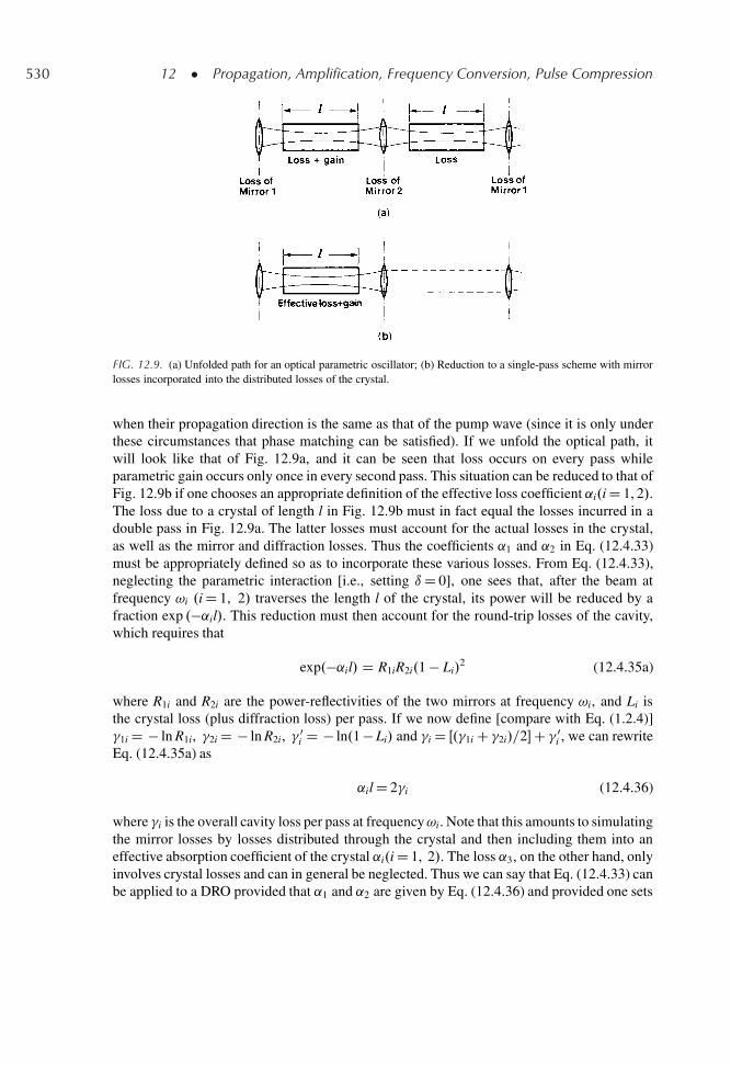
530 12 � Propagation, Amplification, Frequency Conversion, Pulse Compression
FIG. 12.9. (a) Unfolded path for an optical parametric oscillator; (b) Reduction to a single-pass scheme with mirrorlosses incorporated into the distributed losses of the crystal.
when their propagation direction is the same as that of the pump wave (since it is only underthese circumstances that phase matching can be satisfied). If we unfold the optical path, itwill look like that of Fig. 12.9a, and it can be seen that loss occurs on every pass whileparametric gain occurs only once in every second pass. This situation can be reduced to that ofFig. 12.9b if one chooses an appropriate definition of the effective loss coefficient ˛i.i D 1, 2/.The loss due to a crystal of length l in Fig. 12.9b must in fact equal the losses incurred in adouble pass in Fig. 12.9a. The latter losses must account for the actual losses in the crystal,as well as the mirror and diffraction losses. Thus the coefficients ˛1 and ˛2 in Eq. (12.4.33)must be appropriately defined so as to incorporate these various losses. From Eq. (12.4.33),neglecting the parametric interaction [i.e., setting ıD 0], one sees that, after the beam atfrequency !i .i D 1, 2/ traverses the length l of the crystal, its power will be reduced by afraction exp .�˛il/. This reduction must then account for the round-trip losses of the cavity,which requires that
exp.�˛il/ D R1iR2i.1 � Li/2 (12.4.35a)
where R1i and R2i are the power-reflectivities of the two mirrors at frequency !i, and Li isthe crystal loss (plus diffraction loss) per pass. If we now define [compare with Eq. (1.2.4)]�1i D � ln R1i, �2i D � ln R2i, � 0
i D � ln.1 � Li/ and �i D Œ.�1i C �2i/=2�C � 0i , we can rewrite
Eq. (12.4.35a) as
˛il D 2�i (12.4.36)
where �i is the overall cavity loss per pass at frequency!i. Note that this amounts to simulatingthe mirror losses by losses distributed through the crystal and then including them into aneffective absorption coefficient of the crystal ˛i.i D 1, 2/. The loss ˛3, on the other hand, onlyinvolves crystal losses and can in general be neglected. Thus we can say that Eq. (12.4.33) canbe applied to a DRO provided that ˛1 and ˛2 are given by Eq. (12.4.36) and provided one sets
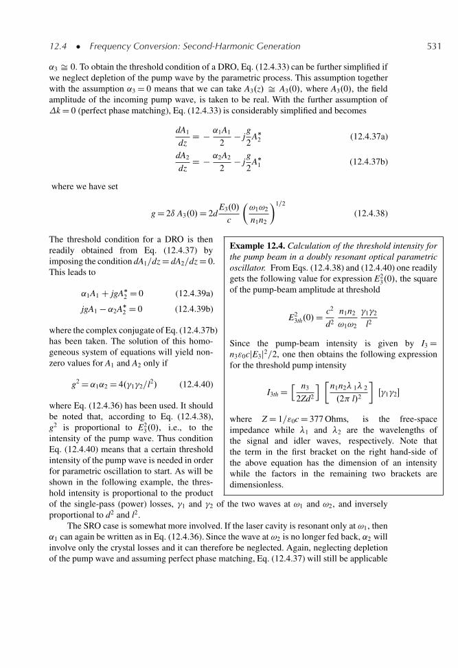
12.4 � Frequency Conversion: Second-Harmonic Generation 531
˛3 Š 0. To obtain the threshold condition of a DRO, Eq. (12.4.33) can be further simplified ifwe neglect depletion of the pump wave by the parametric process. This assumption togetherwith the assumption ˛3 D 0 means that we can take A3.z/ Š A3.0/, where A3.0/, the fieldamplitude of the incoming pump wave, is taken to be real. With the further assumption ofk D 0 (perfect phase matching), Eq. (12.4.33) is considerably simplified and becomes
dA1
dzD � ˛1A1
2� j
g
2A�
2 (12.4.37a)
dA2
dzD � ˛2A2
2� j
g
2A�
1 (12.4.37b)
where we have set
g D 2ı A3.0/D 2dE3.0/
c
�!1!2
n1n2
�1=2
(12.4.38)
Example 12.4. Calculation of the threshold intensity forthe pump beam in a doubly resonant optical parametricoscillator. From Eqs. (12.4.38) and (12.4.40) one readilygets the following value for expression E2
3.0/, the squareof the pump-beam amplitude at threshold
E23th.0/D c2
d2
n1n2
!1!2
�1�2
l2
Since the pump-beam intensity is given by I3 Dn3"0cjE3j2=2, one then obtains the following expressionfor the threshold pump intensity
I3th Dh n3
2Zd2
i �n1n2� 1� 2
.2 l/2
�Œ�1�2�
where Z D 1="0c D 377 Ohms, is the free-spaceimpedance while �1 and �2 are the wavelengths ofthe signal and idler waves, respectively. Note thatthe term in the first bracket on the right hand-side ofthe above equation has the dimension of an intensitywhile the factors in the remaining two brackets aredimensionless.
The threshold condition for a DRO is thenreadily obtained from Eq. (12.4.37) byimposing the condition dA1=dz D dA2=dz D 0.This leads to
˛1A1 C jgA�2 D 0 (12.4.39a)
jgA1 � ˛2A�2 D 0 (12.4.39b)
where the complex conjugate of Eq. (12.4.37b)has been taken. The solution of this homo-geneous system of equations will yield non-zero values for A1 and A2 only if
g2 D ˛1˛2 D 4.�1�2=l2/ (12.4.40)
where Eq. (12.4.36) has been used. It shouldbe noted that, according to Eq. (12.4.38),g2 is proportional to E2
3.0/, i.e., to theintensity of the pump wave. Thus conditionEq. (12.4.40) means that a certain thresholdintensity of the pump wave is needed in orderfor parametric oscillation to start. As will beshown in the following example, the thres-hold intensity is proportional to the productof the single-pass (power) losses, �1 and �2 of the two waves at !1 and !2, and inverselyproportional to d2 and l2.
The SRO case is somewhat more involved. If the laser cavity is resonant only at !1, then˛1 can again be written as in Eq. (12.4.36). Since the wave at !2 is no longer fed back, ˛2 willinvolve only the crystal losses and it can therefore be neglected. Again, neglecting depletionof the pump wave and assuming perfect phase matching, Eq. (12.4.37) will still be applicable
532 12 � Propagation, Amplification, Frequency Conversion, Pulse Compression
provided we now set ˛2 D 0. For small parametric conversion we can set A�1 .z/ Š A�
1 .0/ onthe right-hand side of Eq. (12.4.37b). We thus get
A2.z/D � jgA�1 .0/z=2 (12.4.41)
where the condition A2.0/D 0 has been assumed (i.e., no field, at frequency !2, is fed backinto the crystal by the resonator). If one then substitutes Eq. (12.4.41) in Eq. (12.4.37a) andput A1.z/ Š A1.0/ in the right-hand side of the latter equation, one gets
dA1
dzD�
�˛1
2C g2z
4
�A1.0/ (12.4.42)
Integration of Eq. (12.4.42) over the length, l, of the crystal gives the following expression forthe field at frequency !1
A1.l/D A1.0/
�1 � ˛1l
2C g2l2
8
�(12.4.43)
The threshold condition is then reached when A1.l/D A1.0/, i.e., when
g2 D 4˛1
lD 8�1
l2(12.4.44)
Since g2 is proportional to intensity I of the pump wave, a comparison of Eq. (12.4.44) withEq. (12.4.40) gives the ratio of threshold pump intensities as
ISRO
IDROD 2
�2(12.4.45)
For example, if one takes a loss per pass of �2 D 0.02 (i.e., 2% loss), one finds fromEq. (12.4.45) that the threshold power for the SRO is 100 times larger than for the DRO case.
12.4.2.2. Second-Harmonic Generation
In the case of SHG we take
E.z, t/D .1=2/ fE! expŒj.!t � k!z/�C E2! expŒj.2!t � k2!z/�C c.c.g (12.4.46)
PNL.z, t/D .1=2/˚PNL
! expŒj.!t � k!z/�C PNL2! expŒj.2!t � k2!z/�C c.c.
�(12.4.47)
Substitution of Eqs. (12.4.46) and (12.4.47) into Eq. (12.4.2) gives
PNL2! D "0dE2
! expŒ�j.2k! � k2!/z� (12.4.48a)
PNL! D 2"0dE2!E�
! expŒ�j.k2! � 2k!/z� (12.4.48b)
12.4 � Frequency Conversion: Second-Harmonic Generation 533
If one then substitutes Eq. (12.4.48) into Eq. (12.4.28) and neglects crystal losses (i.e., onetakes �i D 0), one gets
dE2!
dzD � j
!
n2!cdE2
! exp.jkz/ (12.4.49a)
dE!
dzD � j
!
n!cdE2!E�
! exp.�jkz/ (12.4.49b)
where k D k2! � 2k! . These are the basic equations describing SHG.To solve these equations, it is first convenient to define new field variables E0
! and E02! as
E0! D .n!/
1=2 E! (12.4.50a)
E02! D .n2!/
1=2 E2! (12.4.50b)
Since the intensity I! of the wave at ! is proportional to n! jE!j2, the quantity jE0!j2 is seen
to be proportional to I! with a proportionality constant independent of refractive index. Thesubstitution of Eq. (12.4.50) into Eq. (12.4.49) then gives
dE02!
dzD � j
lSH
E02!
E0!.0/
expŒj.kz/� (12.4.51a)
dE0!
dzD � j
lSH
E02!E0�
!
E0!.0/
expŒ�j.kz/� (12.4.51b)
In the above equations E0!.0/ is the value of E0
! at z D 0, assumed to be a real quantity, andlSH is a characteristic length, for second-harmonic interaction, given by
lSH D � .n!n2!/1=2
2 dE!.0/(12.4.52)
where � is the wavelength and E!.0/, the field amplitude of the incident wave at frequency!, is also a real quantity. Note that the advantage of using the new field variables E0
! and E02!
is now apparent from Eq. (12.4.51) since they involve a single coupling parameter, lSH . FromEq. (12.4.51) one readily finds
dˇE0
2!
ˇ2dz
D � d jE0!j2
dz(12.4.53)
which represents the Manley-Rowe relation for SHG. Note that the equation shows that, e.g.,a decrease of beam power, or intensity, at frequency !, must correspond to an increase,by the same amount, of the power or intensity at frequency 2!. Thus 100% conversion offundamental-beam power into second-harmonic power is possible in this case.
As a first example of the solution of Eq. (12.4.51), we consider the case where thereis an appreciable phase mismatch (i.e., lSHk � 1) so that little conversion of fundamentalinto SH is expected to occur. We therefore set E0
!.z/ Š E0!.0/ on the right-hand side of
534 12 � Propagation, Amplification, Frequency Conversion, Pulse Compression
Eq. (12.4.51a). The resulting equation can then be readily integrated and, using the boundarycondition E0
2!.0/D 0, one obtains
E02!.1/D � E0
!.0/
lSH
�exp.�jkl/� 1
k
�(12.4.54)
One can then readily show that
ˇˇE0
2!.l/
E0!.0/
ˇˇ2 D sin2.kl=2/
.klSH=2/2(12.4.55)
Since jE02!j2 is proportional to the SH intensity I2! , the variation of this intensity with crystal
length is immediately obtained from Eq. (12.4.55). The corresponding behavior of I! vs lcan then be obtained from the condition I! C I2! D I!.0/, this condition being an immediateconsequence of Eq. (12.4.53). The plots of ŒI!=I!.0/� and ŒI2!=I!.0/� vs .l=lSH/, obtained inthis way for lSHk D 10, are shown as dashed curves in Fig. 12.10. Note that, due to the largephase mismatch, only a small conversion to second harmonic occurs. Note also that, as canbe readily shown from Eq. (12.4.55), the first maximum of ŒI2!=I!.0/� occurs at l D lc, wherelc, the coherence length, is given by Eq. (12.4.10).
As a second example of a solution to Eq. (12.4.51), we consider the case of perfect phasematching .k D 0/. In this case appreciable conversion to second harmonic may occur andthe depletion of the fundamental beam must therefore be taken into account. This means thatEq. (12.4.51) must now be solved without the approximation E0
!.z/ Š E0!.0/. If k D 0,
however, it can be shown from Eq. (12.4.51) that, if E0!.0/ is taken to be real, then E0
!.z/ andE0
2!.z/ turn out to be real and imaginary, respectively. We can therefore write
E0! D ˇ
E0!
ˇ(12.4.56a)
E02! D � j
ˇE0
2!
ˇ(12.4.56b)
and Eq. (12.4.51) then gives
d jE0! j
dzD � 1
lSH
ˇE0
2!
ˇ jE0! j
E0!.0/
(12.4.57a)
dˇE0
2!
ˇdz
D 1
lSH
jE0! j2
E0!.0/
(12.4.57b)
The solution of Eq. (12.4.57) with the boundary conditions E0!.z D 0/D E0
!.0/ andE0
2!.0/D 0 is
ˇE0
2!
ˇ D E0!.0/ tanh.z=lSH/ (12.4.58a)ˇ
E0!
ˇ D E0!.0/ sech.z=lSH/ (12.4.58b)
Since the intensity of the wave, at a given frequency, is proportional to jE0j2, one hasI2!=I!.0/D jE0
2! j2=E022!.0/ and I!=I!.0/D jE0
!j2=E02! .0/. The dependence of I2!=I!.0/ and
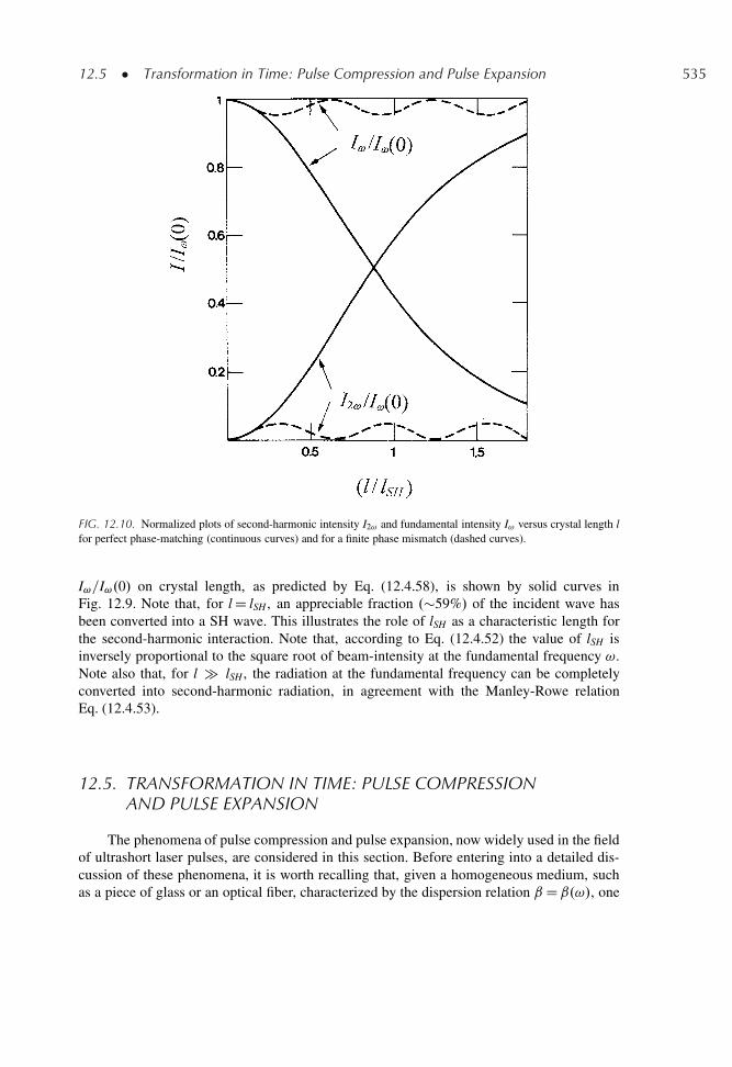
12.5 � Transformation in Time: Pulse Compression and Pulse Expansion 535
FIG. 12.10. Normalized plots of second-harmonic intensity I2! and fundamental intensity I! versus crystal length lfor perfect phase-matching (continuous curves) and for a finite phase mismatch (dashed curves).
I!=I!.0/ on crystal length, as predicted by Eq. (12.4.58), is shown by solid curves inFig. 12.9. Note that, for l D lSH , an appreciable fraction .�59%/ of the incident wave hasbeen converted into a SH wave. This illustrates the role of lSH as a characteristic length forthe second-harmonic interaction. Note that, according to Eq. (12.4.52) the value of lSH isinversely proportional to the square root of beam-intensity at the fundamental frequency !.Note also that, for l � lSH , the radiation at the fundamental frequency can be completelyconverted into second-harmonic radiation, in agreement with the Manley-Rowe relationEq. (12.4.53).
12.5. TRANSFORMATION IN TIME: PULSE COMPRESSIONAND PULSE EXPANSION
The phenomena of pulse compression and pulse expansion, now widely used in the fieldof ultrashort laser pulses, are considered in this section. Before entering into a detailed dis-cussion of these phenomena, it is worth recalling that, given a homogeneous medium, suchas a piece of glass or an optical fiber, characterized by the dispersion relation ˇDˇ.!/, one
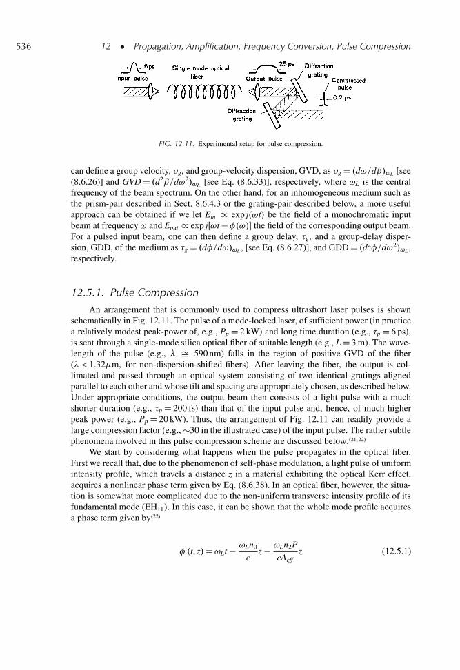
536 12 � Propagation, Amplification, Frequency Conversion, Pulse Compression
FIG. 12.11. Experimental setup for pulse compression.
can define a group velocity, �g, and group-velocity dispersion, GVD, as �g D .d!=dˇ/!L [see(8.6.26)] and GVD D .d2ˇ=d!2/!L [see Eq. (8.6.33)], respectively, where !L is the centralfrequency of the beam spectrum. On the other hand, for an inhomogeneous medium such asthe prism-pair described in Sect. 8.6.4.3 or the grating-pair described below, a more usefulapproach can be obtained if we let Ein / exp j.!t/ be the field of a monochromatic inputbeam at frequency ! and Eout / exp jŒ!t � �.!/� the field of the corresponding output beam.For a pulsed input beam, one can then define a group delay, �g, and a group-delay disper-sion, GDD, of the medium as �g D .d�=d!/!L , [see Eq. (8.6.27)], and GDD D .d2�=d!2/!L ,respectively.
12.5.1. Pulse Compression
An arrangement that is commonly used to compress ultrashort laser pulses is shownschematically in Fig. 12.11. The pulse of a mode-locked laser, of sufficient power (in practicea relatively modest peak-power of, e.g., Pp D 2 kW) and long time duration (e.g., �p D 6 ps),is sent through a single-mode silica optical fiber of suitable length (e.g., L D 3 m). The wave-length of the pulse (e.g., � Š 590 nm) falls in the region of positive GVD of the fiber(�< 1.32�m, for non-dispersion-shifted fibers). After leaving the fiber, the output is col-limated and passed through an optical system consisting of two identical gratings alignedparallel to each other and whose tilt and spacing are appropriately chosen, as described below.Under appropriate conditions, the output beam then consists of a light pulse with a muchshorter duration (e.g., �p D 200 fs) than that of the input pulse and, hence, of much higherpeak power (e.g., Pp D 20 kW). Thus, the arrangement of Fig. 12.11 can readily provide alarge compression factor (e.g., �30 in the illustrated case) of the input pulse. The rather subtlephenomena involved in this pulse compression scheme are discussed below..21,22/
We start by considering what happens when the pulse propagates in the optical fiber.First we recall that, due to the phenomenon of self-phase modulation, a light pulse of uniformintensity profile, which travels a distance z in a material exhibiting the optical Kerr effect,acquires a nonlinear phase term given by Eq. (8.6.38). In an optical fiber, however, the situa-tion is somewhat more complicated due to the non-uniform transverse intensity profile of itsfundamental mode .EH11/. In this case, it can be shown that the whole mode profile acquiresa phase term given by.22/
� .t, z/D!Lt � !Ln0
cz � !Ln2P
cAeffz (12.5.1)
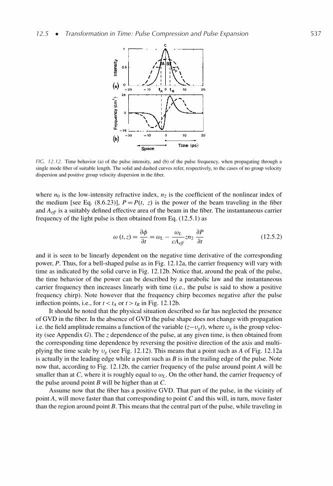
12.5 � Transformation in Time: Pulse Compression and Pulse Expansion 537
FIG. 12.12. Time behavior (a) of the pulse intensity, and (b) of the pulse frequency, when propagating through asingle mode fiber of suitable length. The solid and dashed curves refer, respectively, to the cases of no group velocitydispersion and positive group velocity dispersion in the fiber.
where n0 is the low-intensity refractive index, n2 is the coefficient of the nonlinear index ofthe medium [see Eq. (8.6.23)], P D P.t, z/ is the power of the beam traveling in the fiberand Aeff is a suitably defined effective area of the beam in the fiber. The instantaneous carrierfrequency of the light pulse is then obtained from Eq. (12.5.1) as
! .t, z/D @�
@tD!L � !L
cAeffzn2
@P
@t(12.5.2)
and it is seen to be linearly dependent on the negative time derivative of the correspondingpower, P. Thus, for a bell-shaped pulse as in Fig. 12.12a, the carrier frequency will vary withtime as indicated by the solid curve in Fig. 12.12b. Notice that, around the peak of the pulse,the time behavior of the power can be described by a parabolic law and the instantaneouscarrier frequency then increases linearly with time (i.e., the pulse is said to show a positivefrequency chirp). Note however that the frequency chirp becomes negative after the pulseinflection points, i.e., for t< tA or t> tB in Fig. 12.12b.
It should be noted that the physical situation described so far has neglected the presenceof GVD in the fiber. In the absence of GVD the pulse shape does not change with propagationi.e. the field amplitude remains a function of the variable .z��gt/, where �g is the group veloc-ity (see Appendix G). The z dependence of the pulse, at any given time, is then obtained fromthe corresponding time dependence by reversing the positive direction of the axis and multi-plying the time scale by �g (see Fig. 12.12). This means that a point such as A of Fig. 12.12ais actually in the leading edge while a point such as B is in the trailing edge of the pulse. Notenow that, according to Fig. 12.12b, the carrier frequency of the pulse around point A will besmaller than at C, where it is roughly equal to !L. On the other hand, the carrier frequency ofthe pulse around point B will be higher than at C.
Assume now that the fiber has a positive GVD. That part of the pulse, in the vicinity ofpoint A, will move faster than that corresponding to point C and this will, in turn, move fasterthan the region around point B. This means that the central part of the pulse, while traveling in
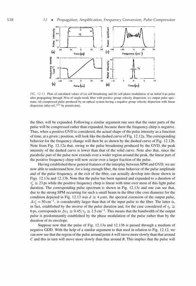
538 12 � Propagation, Amplification, Frequency Conversion, Pulse Compression
FIG. 12.13. Plots of calculated values of (a) self-broadening and (b) self-phase-modulation of an initial 6-ps pulseafter propagating through 30 m of single-mode fiber with positive group velocity dispersion; (c) output pulse spec-trum; (d) compressed pulse produced by an optical system having a negative group velocity dispersion with lineardispersion (after ref.,.21/ by permission).
the fiber, will be expanded. Following a similar argument one sees that the outer parts of thepulse will be compressed rather than expanded, because there the frequency chirp is negative.Thus, when a positive GVD is considered, the actual shape of the pulse intensity as a functionof time, at a given z position, will look like the dashed curve of Fig. 12.12a. The correspondingbehavior for the frequency change will then be as shown by the dashed curve of Fig. 12.12b.Note from Fig. 12.12a that, owing to the pulse broadening produced by the GVD, the peakintensity of the dashed curve is lower than that of the solid curve. Note also that, since theparabolic part of the pulse now extends over a wider region around the peak, the linear part ofthe positive frequency chirp will now occur over a larger fraction of the pulse.
Having established these general features of the interplay between SPM and GVD, we arenow able to understand how, for a long enough fiber, the time behavior of the pulse amplitudeand of the pulse frequency, at the exit of the fiber, can actually develop into those shown inFigs. 12.13a and 12.13b. Note that the pulse has been squared and expanded to a duration of� 0
p Š 23 ps while the positive frequency chirp is linear with time over most of this light pulseduration. The corresponding pulse spectrum is shown in Fig. 12.13c and one can see that,due to the strong SPM occurring for such a small beam in the fiber (the core diameter for thecondition depicted in Fig. 12.13 was d Š 4�m), the spectral extension of the output pulse,�0
L D 50 cm�1, is considerably larger than that of the input pulse to the fiber. The latter is,in fact, established by the inverse of the pulse duration and, for the case considered of �p Š6 ps, corresponds to�L Š 0.45=�p Š 2.5 cm�1. This means that the bandwidth of the outputpulse is predominantly established by the phase modulation of the pulse rather than by theduration of its envelope.
Suppose now that the pulse of Fig. 12.13a and 12.13b is passed through a medium ofnegative GDD. With the help of a similar argument to that used in relation to Fig. 12.12, wecan now see that the region of the pulse around point A will move more slowly than that aroundC and this in turn will move more slowly than that around B. This implies that the pulse will
12.5 � Transformation in Time: Pulse Compression and Pulse Expansion 539
now be compressed. Let us next suppose that the GDD of the medium, besides being negative,is also independent of frequency. According to Eq. (8.6.27), this means that the dispersion ingroup-delay, d�g=d!, will also be negative and independent of frequency. Thus �g decreaseslinearly with frequency and, since the frequency chirp of the pulse increases linearly with time(see Fig. 12.13b), all points of the pulse of Fig. 12.13a will tend to be compressed together atthe same time if the GDD has the appropriate value. According to Eq. (8.6.31), this optimumvalue of GDD must be such that
�d2�
d!2
�!L
!0L D � 0
p (12.5.3)
where !0L D 2 �0
L is the total frequency sweep of the pulse of Fig. 12.13b and � 0p is the
duration of the expanded pulse of Fig. 12.13a. It should be noted, however, that this compres-sion mechanisms cannot produce an indefinitely sharp pulse as, at first sight, one may be ledto believe. In fact, the system providing the negative GDD is a linear medium and this impliesthat the pulse spectrum must remain unchanged on passing through such a system. This meansthat the spectrum of the compressed pulse still remains as that shown in Fig. 12.13c. Evenunder optimal conditions, the duration of the compressed pulse, � 00
p , cannot then be shorterthan approximately the inverse of the spectral bandwidth, i.e., � 00
p Š 1=�0L Š 0.75 ps.
Since the time duration �p of the pulse originally entering the optical fiber was �6 ps (seeFig. 12.11a), the above result indicates that a sizable compression of the incoming light pulsehas been achieved.�
The above heuristic discussion is based on the assumption that a chirped pulse can besubdivided into different temporal regions with different carrier frequencies. Although thisidea is basically correct and allows a description of the phenomena in simple physical terms, amore critical detailed examination of this approach would reveal some conceptual difficulties.To validate this analysis, however, the analytical treatment of the problem can be performedin a rather straightforward way although the intuitive physical picture of the phenomenongets somewhat obscured. For this analytical treatment, in fact, one merely takes the Fouriertransform, E!.!/, of the pulse of Figs. 12.13a and 12.13b and then multiplies, E!.!/, by thetransmission t.!/ of the medium exhibiting negative GDD. The resulting pulse, in the timedomain, is then obtained by taking the inverse Fourier transform of E.!/t.!/. Note that, fora lossless medium, t.!/ must be represented by a pure phase term, i.e., it can be written as
t.!/ D exp.�j�/ (12.5.4)
where �D�.!/. If the medium has a constant GDD, the Taylor-series expansion of �.!/around the central carrier frequency !L gives
�.!/D�.!L/C�
d�
d!
�!L
.! � !L/C 1
2
�d2�
d!2
�!L
.! � !L/2 (12.5.5)
where .d�=d!/!L is the group delay and .d2�=d!2/!L is the group-delay dispersion. By sub-stituting Eq. (12.5.5) into Eq. (12.5.4) and taking the inverse Fourier transform of E.!/t.!/
� Techniques of this type to produce shorter pulses by first imposing a linear frequency chirp followed by pulsecompression have been extensively used in the field of radar (chirped radars) since World War II.
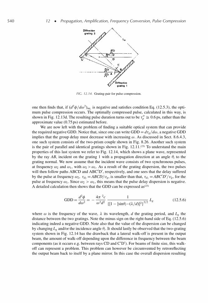
540 12 � Propagation, Amplification, Frequency Conversion, Pulse Compression
FIG. 12.14. Grating-pair for pulse compression.
one then finds that, if .d2�=d!2/!L is negative and satisfies condition Eq. (12.5.3), the opti-mum pulse compression occurs. The optimally compressed pulse, calculated in this way, isshown in Fig. 12.13d. The resulting pulse duration turns out to be � 00
p Š 0.6 ps, rather than theapproximate value (0.75 ps) estimated before.
We are now left with the problem of finding a suitable optical system that can providethe required negative GDD. Notice that, since one can write GDD D d�g=d!, a negative GDDimplies that the group delay must decrease with increasing !. As discussed in Sect. 8.6.4.3,one such system consists of the two-prism couple shown in Fig. 8.26. Another such systemis the pair of parallel and identical gratings shown in Fig. 12.11..23/ To understand the mainproperties of this last system we refer to Fig. 12.14, which shows a plane wave, representedby the ray AB, incident on the grating 1 with a propagation direction at an angle i to thegrating normal. We now assume that the incident wave consists of two synchronous pulses,at frequency !2 and !1, with !2>!1. As a result of the grating dispersion, the two pulseswill then follow paths ABCD and ABC0D0, respectively, and one sees that the delay sufferedby the pulse at frequency !2, �d2 D ABCD=�g, is smaller than that, �d1 D ABC0D0=�g, for thepulse at frequency !1. Since !2 > !1, this means that the pulse delay dispersion is negative.A detailed calculation then shows that the GDD can be expressed as.23/
GDD D d2�
d!2D � 4 2c
!3d2
1
fŒ1 � Œsini�.�=d/�2g3=2Lg (12.5.6)
where ! is the frequency of the wave, � its wavelength, d the grating period, and Lg thedistance between the two gratings. Note the minus sign on the right-hand side of Eq. (12.5.6)indicating indeed a negative GDD. Note also that the value of the dispersion can be changedby changing Lg and/or the incidence angle i. It should lastly be observed that the two-gratingsystem shown in Fig. 12.14 has the drawback that a lateral walk-off is present in the outputbeam, the amount of walk-off depending upon the difference in frequency between the beamcomponents (as it occurs e.g. between rays CD and C0D0). For beams of finite size, this walk-off can represent a problem. This problem can however be circumvented by retroreflectingthe output beam back to itself by a plane mirror. In this case the overall dispersion resulting
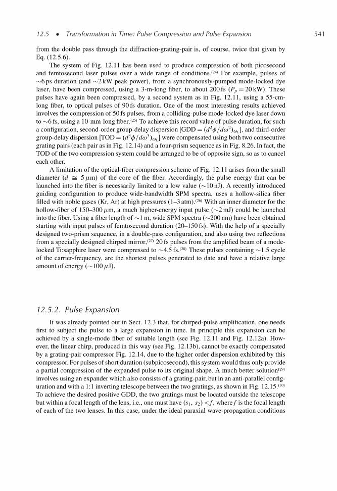
12.5 � Transformation in Time: Pulse Compression and Pulse Expansion 541
from the double pass through the diffraction-grating-pair is, of course, twice that given byEq. (12.5.6).
The system of Fig. 12.11 has been used to produce compression of both picosecondand femtosecond laser pulses over a wide range of conditions..24/ For example, pulses of�6 ps duration (and �2 kW peak power), from a synchronously-pumped mode-locked dyelaser, have been compressed, using a 3-m-long fiber, to about 200 fs .Pp D 20 kW/. Thesepulses have again been compressed, by a second system as in Fig. 12.11, using a 55-cm-long fiber, to optical pulses of 90 fs duration. One of the most interesting results achievedinvolves the compression of 50 fs pulses, from a colliding-pulse mode-locked dye laser downto �6 fs, using a 10-mm-long fiber..25/ To achieve this record value of pulse duration, for sucha configuration, second-order group-delay dispersion ŒGDD D .d2�=d!2/!L �, and third-ordergroup-delay dispersion ŒTOD D .d3�=d!3/!L � were compensated using both two consecutivegrating pairs (each pair as in Fig. 12.14) and a four-prism sequence as in Fig. 8.26. In fact, theTOD of the two compression system could be arranged to be of opposite sign, so as to canceleach other.
A limitation of the optical-fiber compression scheme of Fig. 12.11 arises from the smalldiameter .d Š 5�m/ of the core of the fiber. Accordingly, the pulse energy that can belaunched into the fiber is necessarily limited to a low value .�10 nJ/. A recently introducedguiding configuration to produce wide-bandwidth SPM spectra, uses a hollow-silica fiberfilled with noble gases (Kr, Ar) at high pressures (1–3 atm)..26/ With an inner diameter for thehollow-fiber of 150–300�m, a much higher-energy input pulse .�2 mJ/ could be launchedinto the fiber. Using a fiber length of �1 m, wide SPM spectra .�200 nm/ have been obtainedstarting with input pulses of femtosecond duration .20–150 fs/. With the help of a speciallydesigned two-prism sequence, in a double-pass configuration, and also using two reflectionsfrom a specially designed chirped mirror,.27/ 20 fs pulses from the amplified beam of a mode-locked Ti:sapphire laser were compressed to �4.5 fs..28/ These pulses containing �1.5 cycleof the carrier-frequency, are the shortest pulses generated to date and have a relative largeamount of energy .�100�J/.
12.5.2. Pulse Expansion
It was already pointed out in Sect. 12.3 that, for chirped-pulse amplification, one needsfirst to subject the pulse to a large expansion in time. In principle this expansion can beachieved by a single-mode fiber of suitable length (see Fig. 12.11 and Fig. 12.12a). How-ever, the linear chirp, produced in this way (see Fig. 12.13b), cannot be exactly compensatedby a grating-pair compressor Fig. 12.14, due to the higher order dispersion exhibited by thiscompressor. For pulses of short duration (subpicosecond), this system would thus only providea partial compression of the expanded pulse to its original shape. A much better solution.29/
involves using an expander which also consists of a grating-pair, but in an anti-parallel config-uration and with a 1:1 inverting telescope between the two gratings, as shown in Fig. 12.15..30/
To achieve the desired positive GDD, the two gratings must be located outside the telescopebut within a focal length of the lens, i.e., one must have .s1, s2/< f , where f is the focal lengthof each of the two lenses. In this case, under the ideal paraxial wave-propagation conditions
542 12 � Propagation, Amplification, Frequency Conversion, Pulse Compression
FIG. 12.15. Pulse expander consisting of two diffraction gratings, in an antiparallel configuration, with a 1:1inverting telescope between them.
and negligible dispersion of the lens material, the GDD can be shown to be given by.30/
GDD D d2�
d!2D 4 2c
!3d2 cos2.2f � s1 � s2/ (12.5.7)
where ! is the frequency of the wave, d is the grating period, and is the angle shownin Fig. 12.15. Equation (12.5.7) indeed shows that one has, in this case, a positive value ofGDD. To understand this result we refer again to Fig. 12.15, where the plane wave incident onthe first grating, represented by the ray AB, is assumed to consist of two synchronous pulses,at frequency !2 and !1, with !2>!1. As a result of the grating dispersion, the two pulseswill then follow paths ABCD and ABC0D0, respectively, and one sees that the delay sufferedby the pulse at frequency !2, �d2 D ABCD=�g, is now larger than that, �d1 D ABC0D0=�g, forthe pulse at frequency !1. Since !2 > !1, this means that the pulse delay dispersion is nowpositive. It should be observed that the two-grating telescopic-system shown in Fig. 12.15has the drawback that a lateral walk-off is present in output the beam, the amount of walk-offdepending upon the difference in frequency between the beam components (e.g., between raysCD and C0D0). For beams of finite size, this walk-off can represent a problem. This problemcan however be circumvented by retroreflecting the output beam back to itself by a planemirror. In this case the overall dispersion resulting from the double pass through the systemof Fig. 12.15 is, of course, twice that given by Eq. (12.5.7)
To compare the positive GDD of this pulse expander with the negative GDD of thegrating-pair of Fig. 12.14, we first remember that, according to the grating equation, onehas sin i � .�=d/D sin 0, where i is the angle of incidence at the grating and 0 is the cor-responding diffraction angle. One can now substitute this grating equation into Eq. (12.5.6)and compare the resulting expression with Eq. (12.5.7). One then readily sees that, if 0 D ,the two expressions become identical, apart from having opposite sign, provided that
.Lg=cos /D 2f � s1 � s2 (12.5.8)
It should be stressed that this equivalence only holds under the ideal conditions consideredabove. In this case, and when Eq. (12.5.8) applies, the expander of Fig. 12.15 is said to be con-jugate to the compressor of Fig. 12.14. Physically, the conjugate nature of this expander comesabout from the fact that the telescope produces an image of the first grating which is located
Problems 543
beyond the second grating and parallel to it. The expander of Fig. 12.15 is thus equivalent toa two-parallel-grating system with negative separation and, under condition Eq. (12.5.8), thissystem has exactly opposite dispersion, for all orders, to that of the compressor of Fig. 12.14.In practice, due to lens aberrations and dispersion, the expander of Fig. 12.15 works well forpulse durations larger than �100 fs and for expansion ratios less than a few thousands. Forshorter pulses and larger expansion ratios, the 1:1 telescope of the expander is usually realizedvia a suitably designed cylindrical-.31/ or spherical-mirror configuration..32/ In particular, theuse of the cylindrical-mirror configuration has resulted in an expander with expansion ratiogreater than 104 and with second-, third-, and fourth-order dispersion being matched, for asuitable choice of material dispersion in the amplification chain, to that of the compressor..31/
PROBLEMS
12.1. The Nd:YAG laser beam of example 12.1. is first propagated in free-space for a distance of1 m, starting from its waist, and then focused by a positive lens with f D 10 cm focal length.Calculate the waist position after the lens and the spot-size parameter at this waist. [Hint: Tocalculate this waist position, the lens can be considered to consist of two positive lenses, f1, andf2 .f �1
1 C f �12 D f �1/, the first lens compensating the curvature of the incoming wavefront, thus
producing a plane wave front, while the second focuses the beam: : : .]
12.2. The output of a Q-switched Nd:YAG laser .E D 100 mJ, �p D 20 ns/ is to be amplified by a 6.3-mm-diameter Nd:YAG amplifier having a small signal gain of G0 D 100. Assume that: (1) Thelifetime of the lower level of the transition is much shorter than �p. (2) The beam transverseintensity profile is uniform. (3) The effective peak cross-section for stimulated emission is � Š2.8 � 10�19 cm2. Calculate the energy of the amplified pulse, the corresponding amplification,and the fraction of the stored energy in the amplifier that is extracted by the incident pulse.
12.3. A large Nd: glass amplifier, to be used for amplifying 1-ns laser pulses for fusion experiments,consists of a disk-amplifier with disk clear-aperture of D D 9 cm and overall length of the disks of15 cm. Assume: (1) A measured small signal gain, G0, for this amplifier of � 4. (2) An effective,stimulated-emission peak cross-section for Nd:glass of � D 4 � 10�20 cm2 (see Table 9.3). (3)That the lifetime of the lower level of the transition is much shorter than the laser pulse. Calculatethe total energy available in the amplifier and the required energy of the input-pulse to generatean output energy of Eout D 450 J.
12.4. Following the analysis made in deriving Eqs. (12.3.1) and (12.3.9) (assume ˛D 0) as well asthe rate-equation calculation for a quasi-three level laser [see Eqs. (7.2.21)–(7.2.24)], proveEq. (12.3.15).
12.5. With reference to problem 12.2., assume now that the input pulse duration is much shorter thanthe lifetime, �1, of the lower laser level .�1 Š 100 ps/. Using data obtained in example 2.10.and knowing that the fractional population of the lower laser sub-level of the 4I11=2 state isf13 Š 0.187, calculate the energy of the amplified pulse and the corresponding amplification.Compare the results with those obtained in problem 12.2.
12.6. A large CO2 TEA amplifier (with a gas mixture CO2:N2:He in the proportion 3:1.4:l) hasdimensions of 10 � 10 � 100 cm. The small signal gain coefficient for the P.22/ transitionhas been measured to be g D 4 � 10�2 cm�1. The duration of the input light pulse is 200 ns,
544 12 � Propagation, Amplification, Frequency Conversion, Pulse Compression
which can therefore be assumed much longer than the thermalization time of the rotational lev-els of both the upper and lower vibrational states. The laser pulse is however much shorter thanthe decay time of the lower laser level. The true peak cross-section for the P.22/ transition is� Š 1.54 � 10�18 cm2, while, for T D 300 K, the fractional population of both initial and finalrotational states can be calculated to be f D 0.07. Calculate the output energy and the gain avail-able from this amplifier for an input energy of 17 J. Also calculate the energy per unit volumeavailable in the amplifier.
12.7. Prove Eq. (12.3.12).
12.8. The frequency of a Nd:YAG laser beam .�D 1.06 m/ is to be doubled in a KDP crys-tal. Knowing that, for KDP, no.�D 1.06�m/ D 1.507, no.�D 532 nm/D 1.5283, andne.�D 532 nm/D 1.48222, calculate the phase-matching angle, m.
12.9. Prove Eq. (12.4.30).
12.10. Calculate the threshold pump intensity for parametric oscillation at �1 Š �2 D 1�m in a5-cm-long LiNbO3 crystal pumped at �3 D 0.5�m Œn1 D n2 D 2.16, n3 D 2.24, d Š 6 �10�12 m=V, �1 D �2 D 2 � 10�2�. If the pumping beam is focused in the crystal to a spot of�100 �m diameter, calculate the resulting threshold pump power.
12.11. Calculate the second-harmonic conversion efficiency via type I second-harmonic generation ina perfectly phase-matched 2.5-cm-long KDP crystal for an incident beam at �D 1.06 m havingan intensity of 100 MW=cm2 [for KDP n Š 1.5, deff D d36 sin m D 0.28 � 10�12 m=V, wherem Š 50ı is the phase-matching angle].
References
1. R. W. Boyd, Nonlinear Optics (Academic Press, New York, 1992).2. A. Yariv, Optical Electronics fourth edn. (Holt Rinehart and Winston, New York, 1991), Chaps. 9 and 12.3. O. Svelto, Self-Focusing, Self-Steepening and Self-Phase-Modulation of Laser Beams, in Progress in Optics,
ed. by E. Wolf (North-Holland, Amsterdam 1974), Vol. XII, pp. 3–50.4. A. E. Siegman, New Developments in Laser Resonators, in Laser Resonators ed. by D. A. Holmes, Proc. SPIE,
1224, 2–14 (1990).5. A. E. Siegman, Defining and Measuring Laser Beam Quality, in Solid State Lasers-New Develpments
and Applications, ed. by M. Inguscio and R. Wallenstein (Plenum, New York 1993) pp 13–28.6. L. M. Franz and J. S. Nodvick, Theory of Pulse Propagation in a Laser Amplifier, J. Appl. Phys., 34,
2346–2349 (1963).7. P. G. Kriukov and V. S. Letokhov, Techniques of High-Power Light-Pulse Amplification, in Laser Handbook,
ed. by F. T. Arecchi and E. O. Schultz-Dubois (North-Holland, Amsterdam, 1972), Vol. l, pp. 561–595.8. W. Koechner, Solid-State Laser Engineering, fourth edn. (Springer, Berlin 1996), Chap. 4.9. D. Strickland and G. Mourou, Compression of Amplified Chirped Optical Pulses, Opt. Commun., 56,
219–221 (1985).10. G. Mourou, The Ultra-High-Peak-Power Laser: Present and Future, Appl. Phys. B, 65, 205–211 (1997).11. M. D. Perry et al., The Petawatt Laser and its Application to Inertial Confinement Fusion, CLEO ‘96 Conference
Digest (Optical Society of America, Whashington) paper CWI4.12. Proceedings of the International Conference on Superstrong Fields in Plasmas, ed. by M. Lontano, G. Mourou,
F. Pegoraro, and E. Sindoni (American Institute of Physics Series, New York 1998).13. R. J. Mears, L. Reekie, I. M. Jauncey, and D. N. Payne, Low Noise Erbium-Doped Fiber Amplifier at 1.54�m,
Electron. Lett., 23, 1026–1028 (1987).14. Emmanuel Desurvire, Erbium-Doped Fiber Amplifiers (John Wiley and Sons, New York, 1994).
References 545
15. R. L. Byer, Optical Parametric Oscillators, in Quantum Electronics, ed. by H. Rabin and C. L. Tang (Academic,New York, 1975), Vol. 1, Part B, pp. 588–694.
16. P. A. Franken, A. E. Hill, C. W. Peters, and G. Weinreich, Generation of Optical Harmonics, Phys. Rev. Lett. 7,118 (l961).
17. J. A. Giordmaine and R. C. Miller, Tunable Optical Parametric Oscillation in LiNbO3 at Optical Frequencies,Phys. Rev. Lett. 14, 973 (1965).
18. J. A. Giordmaine, Mixing of Light Beams in Crystals, Phys. Rev. Lett. 8, 19 (1962).19. P. D. Maker, R. W. Terhune, M. Nisenhoff, and C. M. Savage, Effects of Dispersion and Focusing on the
Production of Optical Harmonics, Phys. Rev. Lett. 8, 21 (l962).20. F. Zernike and J. E. Midwinter, Applied Nonlinear Optics (Wiley, New York, 1973), Sec. 3.7.21. D. Grischkowsky and A. C. Balant, Optical Pulse Compression Based on Enhanced Frequency Chirping, Appl.
Phys. Lett. 41, 1 (1982).22. G. P. Agrawal, Nonlinear Fiber Optics, second edn. (Academic, San Diego, 1995) Chapter 2.23. E. B. Treacy, Optical Pulse Compression with Diffraction Gratings, IEEE J. Quantum Electron. QE-5,
454 (1969).24. Reference [22] Chapter 6.25. R. L. Fork et al., Compression of Optical Pulses to Six Femtosecond by Using Cubic Phase Compensation, Opt.
Lett., 12, 483–485 (1987).26. M. Nisoli, S. De Silvestri and O. Svelto, Generation of High Energy 10 fs Pulses by a New Compression
Technique, Appl. Phys. Letters, 68, 2793–2795 (1996).27. R. Szipocs, K. Ferencz, C. Spielmann, F. Krausz, Chirped Multilayer Coatings for Broadband Dispersion Control
in Femtosecond Lasers, Opt. Letters, 19, 201–203 (1994).28. M. Nisoli et al., Compression of High-Energy Laser Pulses below 5 fs, Opt. Letters, 22, 522–524 (1997).29. M. Pessot, P. Maine and G. Mourou, 1000 Times Expansion-Compression Optical Pulses for Chirped Pulse
Amplification, Opt. Comm., 62, 419–421 (1987).30. O. E. Martinez, 3000 Times Grating Compressor with Positive Group Velocity Dispersion: Application to Fiber
Compensation in 1.3–1.6�m Region, IEEE J. Quantum Electron., QE-23, 59–64 (1987).31. B. E. Lemoff and C. P. J. Barty, Quintic-Phase-Limited, Spatially Uniform Expansion and Recompression of
Ultrashort Optical Pulse, Opt. Letters, 18, 1651–1653 (1993).32. Detao Du et al., Terawatt Ti:Sapphire Laser with a Spherical Reflective-Optic Pulse Expander, Opt. Letters, 20,
2114–2116 (1995).
A
Semiclassical Treatmentof the Interaction of Radiationwith Matter
The calculation that follows will make use of the so-called semiclassical treatment of theinteraction of radiation with matter. In this treatment the atomic system is assumed to be quan-tized and it is therefore described quantum mechanically while the e.m. radiation is treatedclassically, i.e., by using Maxwell’s equations.
We will first examine the phenomenon of absorption. We therefore consider the usualtwo-level system where we assume that, at time t D 0, the atom is in its ground state 1 andthat a monochromatic e.m. wave at frequency! made to interact with it. Classically, the atomhas an additional energy H0 when interacting with the e.m. wave. For instance this may bedue to the interaction of the electric dipole moment of the atom μe with the electric field Eof the e.m. wave .H0 D μe � E/, referred to as as an electric dipole interaction. This is notthe only type of interaction through which the transition can occur, however. For instance,the transition may result from the interaction of the magnetic dipole moment of the atom μm
with the magnetic field B of the e.m. wave (μm � B, magnetic dipole interaction). To describethe time evolution of this two-level system, we must now resort to quantum mechanics. Thus,just as the classical treatment involves an interaction energy H0, so the quantum mechanicalapproach introduces an interaction Hamiltonian H 0. This Hamiltonian can be obtained fromthe classical expression for H0 according to the well-known rules of quantum mechanics. Theprecise expression for H 0 need not concern us at this point, however. We only need to notethat H 0 is a sinusoidal function of time with frequency equal to that of the incident wave.Accordingly we put
H 0 D H00 sin !t (A.1)
The total Hamiltonian H for the atom can then be written as
H D H0 C H 0 (A.2)
547
548 Appendixes
where H0 is the atomic Hamiltonian in the absence of the e.m. wave. Once the totalHamiltonian H for t > 0 is known, the time evolution of the wave function of the atom isobtained from the time-dependent Schrodinger equation
H D j„@ @ t
(A.3)
To solve Eq. (A.3) for the wave-function .t/ we begin by introducing, accordingto Eq. (2.3.1), 1 D u1 expŒ�.jE1t=„/� and 2 D u2 expŒ�.jE2t=„/�, as the unperturbedeigenfunctions of levels 1 and 2, respectively. Thus u1 and u2 satisfy the time-independentSchrodinger wave-equation
H0ui D Ei ui .i D 1, 2/ (A.4)
Under the influence of the e.m. wave, the wave-function of the atom can be written as
D a1.t/ 1 C a2.t/ 2 (A.5)
where a1 and a2 will be time-dependent complex numbers that, according to quantummechanics, obey the relation
ja1j2 C ja2j2 D 1 (A.6)
Since, according to Eq. (1.1.6), one has W12 D �dja1.t/j2=dt D dja2.t/j2=dt, to calculateW12, we must calculate the function ja2.t/j2. To do this we will first generalize Eq. (A.5) as
DmX1
ak k DmX1
ak uk expŒ�j.Ek=„/ t� (A.7)
where k denotes a general state of the atom and m gives the number of these states. Bysubstituting Eq. (A.7) into Eq. (A.3) we obtain
Pk.H0 C H 0/ak uk expŒ�j.Ek=„/ t� D P
kfj „.dak=dt/uk expŒ�j.Ek=„/ t�
C akukEk expŒ�j .Ek=„/ t�g(A.8)
This equation, with the help of Eq. (A.4), reduces to
Xj„.dak=dt/uk expŒ�j.Ek=„/ t� D
XakH
0uk expŒ�j.Ek=„/ t� (A.9)
By multiplying each side of this equation by the arbitrary eigenfunction u�n and then
integrating over the whole space, we obtain
Pj„.dak=dt/ expŒ�j.Ek=„/ t�
Ruk u�
n dV
D Pak expŒ�j.Ek=„/t�
Ru�
n H 0uk dV(A.10)
Appendix A 549
Since the wave functions uk are orthogonal (i.e.,R
u�n uk dV D ıkn), Eq. (A.10) gives
.dan=dt/ D 1
.j„/mX1
kH0nkak exp
��j.Ek � En/t
„�
(A.11)
where H0nk D H0
nk.t/ is given by
H0nk.t/ D
Zu�
n H 0 uk dV (A.12)
Equation (A.11) comprises a set of m differential equations for the m variables ak.t/, andthese equations can be solved once the initial conditions are known. For the simpler case ofa two-level system the wave-function is given by Eqs. (A.5) and (A.11) reduces to the twoequations
�da1
dt
�D�
1
j„� n
H011 a1 C H0
12 a2 exph�j.E2 � E1/
t
„io
(A.13a)
�da2
dt
�D�
1
j„� n
H021 a1 exp
h�j.E1 � E2/
t
„i
C H022 a2
o(A.13b)
which are to be solved with the initial condition a1.0/ D 1, a2.0/ D 0.So far, no approximations have been made. Now, to simplify the solution of the
Eq. (A.13), we will make use of a perturbation method. We will assume that on the right-hand side of Eq. (A.13) we can make the approximations that a1.t/ Š 1 and a2.t/ Š 0. Bysolving Eq. (A.13) subject to this approximation, we obtain the first-order solutions for a1.t/and a2.t/. For this reason, the theory that follows is known as first-order perturbation theory.The solutions a1.t/ and a2.t/ obtained in this way can then be substituted in the right-handside of Eq. (A.13) to get a solution which could then be a second-order approximation, and soon to higher orders. To first order, therefore, Eq. (A.13) gives
�da1
dt
�D�
1
j„�
H011 (A.14a)
�da2
dt
�D�
1
j„�
H021 exp .j!0t/ (A.14b)
where we have written !0 D .E2�E1/=„ for the transition frequency of the atom. To calculatethe transition probability, we need only to solve Eq. (A.14b). Thus, making use of Eqs. (A.1)and (A.12), we write
H021 D H00
21 sin! t D H0021Œexp.j! t/ � exp.�j! t/�=2j (A.15)
where H0021 is given by
H0021 D
Zu�
2 H00u1 dV (A.16)
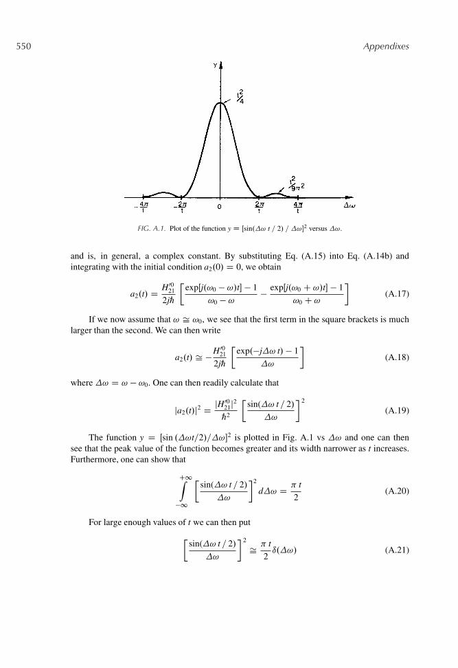
550 Appendixes
FIG. A.1. Plot of the function y D Œsin.! t = 2/ = !�2 versus !.
and is, in general, a complex constant. By substituting Eq. (A.15) into Eq. (A.14b) andintegrating with the initial condition a2.0/ D 0, we obtain
a2.t/ D H0021
2j„�
expŒj.!0 � !/t� � 1
!0 � !� expŒj.!0 C !/t� � 1
!0 C !
�(A.17)
If we now assume that ! Š !0, we see that the first term in the square brackets is muchlarger than the second. We can then write
a2.t/ Š �H0021
2j„�
exp.�j! t/ � 1
!
�(A.18)
where ! D ! � !0. One can then readily calculate that
ja2.t/j2 D jH0021j2
„2
�sin(! t = 2/
!
� 2
(A.19)
The function y D Œsin .!t=2/=!�2 is plotted in Fig. A.1 vs ! and one can thensee that the peak value of the function becomes greater and its width narrower as t increases.Furthermore, one can show that
C1Z�1
�sin(! t = 2/
!
�2
d! D t
2(A.20)
For large enough values of t we can then put
�sin(! t = 2/
!
� 2
Š t
2ı.!/ (A.21)
Appendix A 551
where ı is the Dirac ı function. Within this approximation Eq. (A.19) gives
ja2.t/j2 D jH0021j2
„2
2tı.!/ (A.22)
which shows that, for long enough times, the probability ja2.t/j2 of finding the atom in leveltwo is proportional to the time t. Consequently, the transition probability W12 is obtained as
W12 D dja2.t/j2
dtD
2
jH0021j2
„2ı.!/ (A.23)
To calculate W12 explicitly, we must now calculate the quantityˇH00
21
ˇ2. Let us assume
that the interaction responsible for the transition occurs between the electric field of the e.m.wave and the electric dipole moment of the atom (electric-dipole interaction). Classically, ifwe let r be the vector that specifies the position of the electron with respect to the nucleus ande the magnitude of the electron charge, the corresponding dipole moment of the atom will beμe D �er. The classical interaction energy H0 is then given by H0 D μe � E D �eE.r, t/ � r,where E is the electric field of the incident e.m. wave at the electron position. Following thewell-known rules of quantum mechanics, the interaction Hamiltonian is then simply given by
H 0 D �eE.r, t/ � r (A.24)
Substitution of Eq. (A.24) into Eq. (A.12) with n D 2 and k D 1, gives
H021 D �e
Zu�
2 E � r u1 dV (A.25)
Let us now suppose that the wavelength of the e.m. wave is much larger than the atomicdimension. This is satisfied very well for e.m. waves in the visible. One has in fact � D 500 nmfor green light while typical atomic dimensions are � 0.1 nm). In this case, we can assumethat E(r, t) does not change appreciably over an atomic dimension and thus remains equal toits value, E(0, t), at r D 0, i.e., at the center of the nucleus (electric-dipole approximation).We can thus write
E.r, t/ Š E.0, t/ D E0 sin!t (A.26)
where E0 is a constant. If Eq. (A.26) is now substituted into Eq. (A.25) and the result-ing expression for H0
21 compared with that given in Eq. (A.15), one finds that H0021 can be
expressed as
H0021 D E0 � μ21 (A.27)
where μ21 is given by
μ21 D �Z
u�2 eru1 dV (A.28)
552 Appendixes
and is called the matrix element of the electric dipole moment. If we now let as cos be theangle between μ21 and E0 we obtain from Eq. (A.27) that
ˇH00
21
ˇ2 D E20 j�21j2 cos2 (A.29)
where j�21j is the magnitude of the complex quantity μ21. If we now assume that the e.m.wave interacts with several atoms whose vectors μ21 are randomly oriented with respect to E0,the average value of
ˇH00
21
ˇ2will be obtained by averaging Eq. A.29 over all possible angles
and � (in two dimensions). To carry this out, let p.) represent the probability density forthe orientation of the atomic dipoles, so that p./d˝ gives the elemental probability thatthe vector μ21 is within the solid angle d˝ making an angle with the direction of E0. Forrandomly oriented dipoles, one has p./ D const. and accordingly one has< cos2 >D 1=3,where the brackets<> indicate the average value over all dipole orientations. From Eq. (A.29)we then get
˝jH0021j2
˛ D E20j�21j2=3 (A.30)
The substitution of this last expression into Eq. (A.23) then gives
W12 D
6
.2 /2E20j�21j2
h2ı.! � !0/ (A.31)
If the function ı.v�v0/ is used instead of ı.!�!0/ in Eq. (A.31) then, since ı.v�v0/ D2 ı.! � !0/, Eq. (A.31) transforms to Eq. (2.4.5).
Having calculated the rate of absorption, we can now go on to calculate the rate ofstimulated emission. To do this, we should start again from Eq. (A.13), this time usingthe initial conditions a1.0/ D 0 and a2.0/ D 1. We immediately see, however, that therequired equations in this case are obtained from the corresponding Eqs. [(A.13)–(A.31)] forthe case of absorption simply by interchanging the indexes 1 and 2. Since it can be seen fromEq. (A.28) that j�12j D j�21j, it follows from Eq. (A.31) that W12 D W21, which shows thatthe probabilities of absorption and stimulated emission are equal.
B
Lineshape Calculation for CollisionBroadening
As explained in Sect. 2.5.1, the calculation of the lineshape for collision broadening can beobtained from the normalized spectral density, g.�0 � �/, of the sinusoidal waveform withrandom phase-jumps shown in Fig. 2.9. The signal wave of Fig. 2.9 will be written as
E.t/ D E0 exp jŒ!t � �.t/� (B.1)
where E0 is taken to be a real constant, ! D 2 � is the angular frequency of the radiationand where the phase �.t/ is assumed to undergo random jumps at each atom’s collision.We will assume that the probability density, p� .�/, of the time � between two consecutivecollisions can be described by Eq. (2.5.7). The calculation of g.�0 � �/ is best done in termsof the angular frequency !, i.e., in terms of the distribution, g.!0 � !/. Since obviouslyone has g.�0 � �/d �0 D g.!0 � !/d!0, it follows that g.�0 � �/ D 2 g.!0 � !/. Apartfrom a proportionality constant, the function g.!0 � !/ is then given by the power spectrumW.!0 � !/ of the waveform shown in Fig. 2.9. For this proportionality constant to be unity,we require, according to Eq. (2.5.4), that W.!0 �!/ be such that s W.!0 �!/d !0 D 1. FromParseval’s theorem one then has
C1Z�1
W.!0 � !/d!0 D limT!1
T
CTZ�T
jE.t/j2dt D 2 E20 (B.2)
The condition s W.!0 � !/d!0 D 1 then leads to the result 2 E20 D 1. This means that
g.!0 � !/ can be obtained as the power spectrum of the signal E.t/ given by Eq. (B.1) andwith amplitude
E0 D .2 /�1=2 (B.3)
553
554 Appendixes
To calculate the power spectrum W.!0 � !/ of the signal given in Eq. (B.1) we make use ofthe Wiener-Kintchine theorem so that W.!0 � !/ is obtained as the Fourier transform of thesignal autocorrelation function, � .�/. We can thus write
W.!0 � !/ DC1Z
�1� .�/ exp �.j!0�/ d� (B.4)
where the autocorrelation function � .�/ is given by
� .�/ D limT!1
1
2T
CTZ�T
E�.t/E.t C �/dt (B.5)
For the waveform shown in Fig. 2.9, we can then write
� .�/ D limT!1
1
2TE2
0 exp.j!�/
8<:Z
corr.
dt CZ
uncorr.
expŒ�j.�/�dt
9=; (B.6)
The first integral in the right hand side of Eq. (B.6) is calculated over the time intervals,between �T and CT, in which no phase-jumping collision has occurred and thus the signalsE.t/ and E.t C �/ have the same phase (correlated intervals). The second integral in the righthand side of Eq. (B.6) is calculated over the time intervals in which a collision has occurredand thus the two signals E.t/ and E.t C �/ have a random phase difference� (uncorrelatedintervals). This situation can be illustrated schematically as in Fig. B.1, where the vertical bars(continuous-line) indicate the instants of phase jumps for both E.t/ and E.tC�/. On projectingthe vertical bars of e.g., E.t C �/ onto the plot of E.t/ (dashed vertical lines), the correlatedtime intervals, shown as hatched areas, are obtained.
To calculate � .�/ from Eq. (B.6) we first notice that the contribution of the secondintegral in the right hand side of Eq. (B.6) vanishes as T tends to infinite because the integrandexpŒ�j.�/� is a random number with zero average. Equation (B.6) then reduces to
� .�/ D limT!1
E20
2Texp.j!�/
24 Z
corr.
dt
35 (B.7)
The integral in Eq. (B.7) is equal to the total time of phase correlation, i.e. to the sums ofthe time intervals corresponding to the hatched areas in Fig. B.1. If we let � 0
n represent thetime interval between the n-th phase-jump and the next one (see Fig. B.1), this sum can beexpressed as
Pn
� 0
n � ��, where summation is extended over the values � 0n for which � 0
n > � .Equation (B.7) can then be written as
� .�/ D E20 exp.j!�/ lim
T!1
Pn .�
0n � �/
2T(B.8)
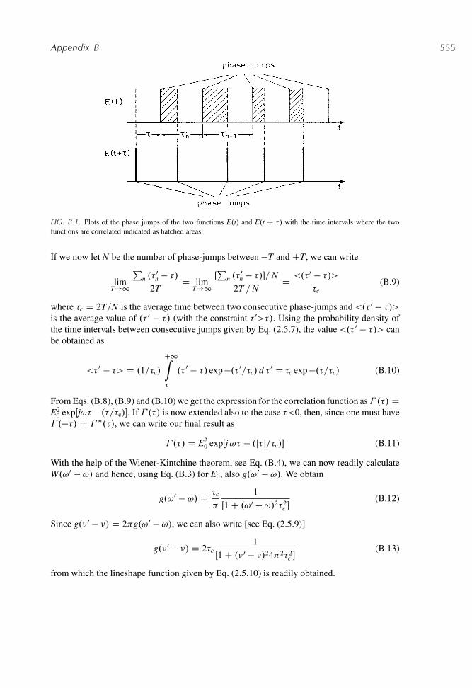
Appendix B 555
FIG. B.1. Plots of the phase jumps of the two functions E.t/ and E.t C �/ with the time intervals where the twofunctions are correlated indicated as hatched areas.
If we now let N be the number of phase-jumps between �T and CT, we can write
limT!1
Pn .�
0n � �/
2TD lim
T!1ŒP
n .�0n � �/�=N
2T =ND <.� 0 � �/>
�c(B.9)
where �c D 2T=N is the average time between two consecutive phase-jumps and <.� 0 � �/>is the average value of .� 0 � �/ (with the constraint � 0>�/. Using the probability density ofthe time intervals between consecutive jumps given by Eq. (2.5.7), the value <.� 0 � �/> canbe obtained as
<� 0 � �> D .1=�c/
C1Z�
.� 0 � �/ exp �.� 0=�c/ d � 0 D �c exp �.�=�c/ (B.10)
From Eqs. (B.8), (B.9) and (B.10) we get the expression for the correlation function as� .�/ DE2
0 expŒj!� � .�=�c/�. If � .�/ is now extended also to the case �<0, then, since one must have� .��/ D � �.�/, we can write our final result as
� .�/ D E20 expŒj!� � .j� j=�c/� (B.11)
With the help of the Wiener-Kintchine theorem, see Eq. (B.4), we can now readily calculateW.!0 � !/ and hence, using Eq. (B.3) for E0, also g.!0 � !/. We obtain
g.!0 � !/ D �c
1
Œ1 C .!0 � !/2�2c �
(B.12)
Since g.�0 � �/ D 2 g.!0 � !/, we can also write [see Eq. (2.5.9)]
g.�0 � �/ D 2�c1
Œ1 C .�0 � �/24 2�2c �
(B.13)
from which the lineshape function given by Eq. (2.5.10) is readily obtained.
C
Simplified Treatment of AmplifiedSpontaneous Emission
We will assume that ASE emission occurs in both directions within the active medium andtherefore refer to the geometry shown in Fig. C.1. We will further assume that the amplifierbehaves as an ideal four-level system, so that the lower level population can be neglected. Wewill consider both homogeneously and inhomogeneously broadened transitions. A detailedtheory that holds for these conditions has been developed by Casperson..1/ The theory is rathercomplicated, however, and as a result one cannot readily obtain the main aspects of the phys-ical behavior of ASE from this treatment. Following some very recent work,.2/ we presenthere a simplified treatment of ASE aimed at obtaining some asymptotic expressions for ASEbehavior in the low saturation regime.
In the low saturation regime, we assume that the upper state population, N2, and hencethe population inversion N Š N2, are not appreciably saturated by the ASE intensity. Withreference to Fig. C.1, we let I�.z, �/ be the spectral ASE intensity at coordinate z for the beampropagating in the positive z-direction. The elemental variation, dI� , along the z-coordinate,must account not only for the stimulated emission but also for the spontaneous-emissioncontribution arising from the element dz. We can thus write
@ I�
@ zD �NI� C NA�
˝.z/
4 (C.1)
where � is the transition cross section at frequency �, A� is the rate of spontaneous emissionat frequency � and˝.z/ is the solid angle subtended by the exit face as seen from the elementdz. Note that the factor ˝.z/=4 , in the right hand side of Eq. (C.1), accounts for the factthat the spontaneous radiation from the element dz is emitted uniformly over the whole solidangle, 4 , while we are only interested in that fraction emitted within the solid angle ˝.z/.To calculate the ASE spectral intensity I�.l, �/ at the z D l exit face of the medium, wemust integrate Eq. (C.1) over the z-coordinate. Noting that most of ASE emission arises fromemitting elements near z D 0, which experience the largest gain, we can assume ˝.z/ Š ˝ ,
557
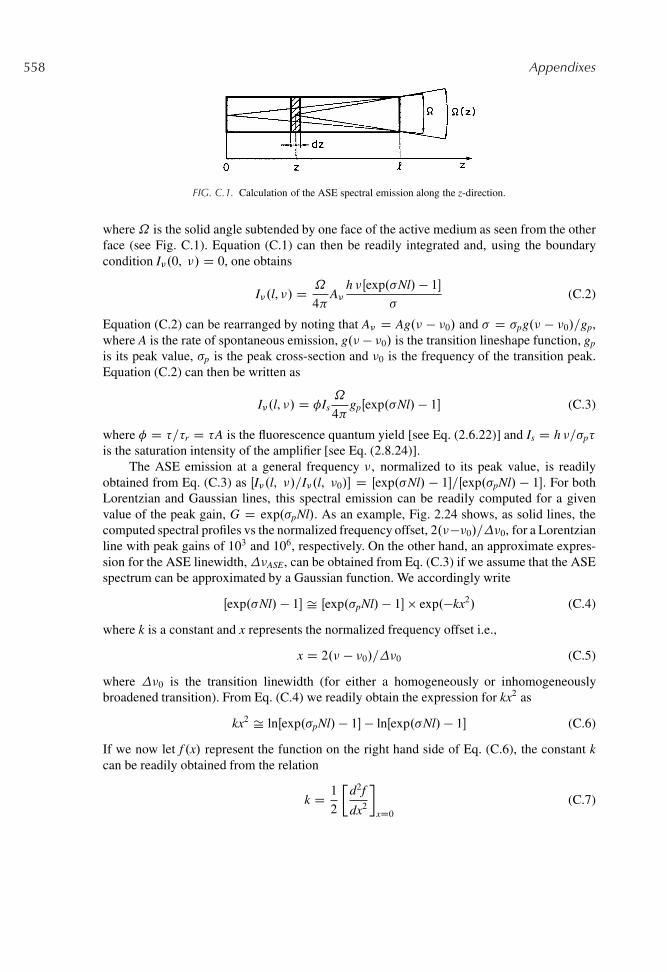
558 Appendixes
FIG. C.1. Calculation of the ASE spectral emission along the z-direction.
where˝ is the solid angle subtended by one face of the active medium as seen from the otherface (see Fig. C.1). Equation (C.1) can then be readily integrated and, using the boundarycondition I�.0, �/ D 0, one obtains
I�.l, �/ D ˝
4 A�
h �Œexp.�Nl/ � 1�
�(C.2)
Equation (C.2) can be rearranged by noting that A� D Ag.� � �0/ and � D �pg.� � �0/=gp,where A is the rate of spontaneous emission, g.� � �0/ is the transition lineshape function, gp
is its peak value, �p is the peak cross-section and �0 is the frequency of the transition peak.Equation (C.2) can then be written as
I�.l, �/ D �Is˝
4 gpŒexp.�Nl/� 1� (C.3)
where � D �=�r D �A is the fluorescence quantum yield [see Eq. (2.6.22)] and Is D h �=�p�
is the saturation intensity of the amplifier [see Eq. (2.8.24)].The ASE emission at a general frequency �, normalized to its peak value, is readily
obtained from Eq. (C.3) as ŒI�.l, �/=I�.l, �0/� D Œexp.�Nl/ � 1�=Œexp.�pNl/ � 1�. For bothLorentzian and Gaussian lines, this spectral emission can be readily computed for a givenvalue of the peak gain, G D exp.�pNl/. As an example, Fig. 2.24 shows, as solid lines, thecomputed spectral profiles vs the normalized frequency offset, 2.���0/=�0, for a Lorentzianline with peak gains of 103 and 106, respectively. On the other hand, an approximate expres-sion for the ASE linewidth,�ASE, can be obtained from Eq. (C.3) if we assume that the ASEspectrum can be approximated by a Gaussian function. We accordingly write
Œexp.�Nl/ � 1� Š Œexp.�pNl/� 1� � exp.�kx2/ (C.4)
where k is a constant and x represents the normalized frequency offset i.e.,
x D 2.� � �0/=�0 (C.5)
where �0 is the transition linewidth (for either a homogeneously or inhomogeneouslybroadened transition). From Eq. (C.4) we readily obtain the expression for kx2 as
kx2 Š lnŒexp.�pNl/� 1�� lnŒexp.�Nl/� 1� (C.6)
If we now let f .x/ represent the function on the right hand side of Eq. (C.6), the constant kcan be readily obtained from the relation
k D 1
2
�d2f
dx2
�xD0
(C.7)
Appendix C 559
For a Lorentzian line, we now write � D �p=.1 C x2/ in Eq. (C.6). After some lengthy butstraightforward calculations, we then get from Eq. (C.7)
k D G ln G
.G � 1/(C.8)
Similarly, for the case of a Gaussian line, we write � D �p exp �.x2 ln 2/ in Eq. (C.6) andthus obtain from Eq. (C.7)
k D .ln 2/G ln G
.G � 1/(C.9)
With the above Gaussian approximation, the normalized ASE linewidth, in terms of the nor-malized frequency offset x, is now readily obtained as xASE D 2.ln 2=k/1=2. Since, fromEq. (C.5), one has�ASE D xASE � .�0=2/, the ASE linewidth can be found from the twoprevious expressions once the value for k given by Eq. (C.8) or (C.9) is used. We thus obtain
�ASE D Œln 2�1=2
�G � 1
G ln G
�1=2
�0 (C.10)
for a Lorentzian line and
�ASE D�
G � 1
G ln G
�1=2
�0 (C.11)
for a Gaussian line. As an example, expression Eq. (C.10) has been used to obtain the nor-malized ASE linewidth, �ASE=�0, vs peak gain G which is plotted in Fig. 2.25 as adashed line.
With the help of these considerations on the spectral behaviour of ASE, we can now alsoobtain an approximate expression for the total ASE intensity, I D s I�d�, at the exit face ofthe active medium. To obtain this we first integrate both sides of Eq. (C.3) over frequency �and obtain
I D � Is
�˝
4
�gp
C1Z�1
Œexp.�Nl/� 1�d� (C.12)
With the help of the Gaussian approximation for the ASE spectrum given by Eq. (C.4), theintegral in Eq. (C.12) is readily calculated, using Eqs. (C.8) and (C.9), to give [see Eq. (2.9.3)]
I D � Is
�˝
4 3=2
�.G � 1/3=2
ŒG ln G�1=2(C.13)
for a Lorentzian and
I D � Is
�˝
4
�.G � 1/3=2
ŒG ln G�1=2(C.14)
for a Gaussian line.

560 Appendixes
References
1. L.W. Casperson, Threshold Characteristics of Mirrorless Lasers, J. Appl. Phys. 48, 256 (1977)2. O. Svelto, S. Taccheo, and C. Svelto, Analysis of Amplified Spontaneous Emission: Some Corrections to the
Lindford Formula, Opt. Comm. 149, 277–282 (1998)
D
Calculation of the Radiative TransitionRates of Molecular Transitions
A simplified treatment is considered here merely to show how the selection rules arise for amolecular transition.
The transition probability can be expressed in the form of Eq. (2.4.9) provided that theappropriate value for the amplitude of the oscillating dipole moment j�j is used. Thus webegin by recalling that, for an ensemble of negative charges (the electrons of the molecule),each of value e (with the sign included) and of positive charges of value eh (the nuclei of themolecule) the classical electrical dipole moment is given by μ D †i eri C†j eh Rj. Here, ri
and Rj specify the positions of the electrons and of the nuclei, respectively, relative to somegiven reference point, and the sum is taken over all electrons and nuclei of the molecule. Ifthe reference point is taken to be center of the positive charges, then †j eh Rj D 0 and μ
reduces to
μ D †i eri (D.1)
To simplify matters, we will now consider a diatomic molecule. In this case the nuclearcoordinates may be reduced to the magnitude R of the internuclear spacing R and to the angu-lar coordinates, , and, �, of R relative to a given reference system. According to quantummechanics the oscillating dipole moment of the molecule is then given by [see also Eq. (2.3.6)]
μosc D 2 ReZ �
2 .ri, R, rr/ μ 1 .ri, R, rr/ dri dR drr (D.2)
where 2 and 1 are, respectively, the wave functions of the final and initial states of thetransition. Note that both 1 and 2 are taken to be functions of the positions of all electrons,of the internuclear distance R, and of the rotational coordinates rr (a shorthand notation for and �), and the integral is taken over all these coordinates. Following the Born-Oppenheimer
561
562 Appendixes
approximation, the molecular wave functions can now be written as
.ri, R, rr/ D ue.ri, R/ u�.R/ ur.rr/ exp Œ�j .E =„/ t� (D.3)
where ue, u� , and ur are the electronic, vibrational, and rotational wave functions, respec-tively, and E D Ee C E� C Er is the total energy of the given state. The substitution ofEq. (D.3) into Eq. (D.2) then shows that μosc oscillates at the frequency �21 D .E2 � E1/=hwith a complex amplitude μ21 given by [compare with Eq. (2.3.7)]
μ21 D�Z
u��2 μe u�1 dR
� �Zu�
r2 ur1 drr
�(D.4)
In the above expression one has
μe D μe.R/ DZ
u�e2.ri, R/μ ue1.ri, R/ dri (D.5)
where μ is the dipole moment given by Eq. (D.1). Since the electronic wave functions areslowly varying functions of R, μe.R/ can then be expanded in a power series around theequilibrium internuclear distance R0 in the form
μe.R/ D μe.R0/C dμe
dR.R � R0/C : : : (D.6)
Let us first consider pure rotational transitions. In this case one has ue2 D ue1 and u�2 Du�1 and, from Eq. (D.5), the dipole moment μe.R0/ is seen to be given by
μe.R0/ DZ
μ jue1.ri, R0/j2 dri (D.7)
which is the permanent electric dipole moment μep of the molecule. If we assume μ D μe.R0/
in the first integral on the right hand side of Eq. (D.4) and remember thatR
u��2 u�1 dR DR ju�1j2 dR D 1, we get the following expression for j�21j2 D jμ21j2 to be used in Eq. (2.4.9):
j�21j2 D jμepj2
ˇˇZ
u�r2ur1drr
ˇˇ2
(D.8)
The first factor in the right-hand side of Eq. (D.8) indicates that pure rotational transi-tions are possible only in molecules possessing a permanent dipole moment μep. This can beeasily understood because the stimulated emission process can be considered to arise from theinteraction of the incident e.m. wave with this rotating dipole moment. For molecules with apermanent dipole moment, j�21j2 is then proportional to the second factor on the right-handside of Eq. (D.8). From the symmetry properties of the rotational wave functions, it then fol-lows that this factor is nonzero only if the quantum jump J between the rotational numbersof the two states obeys the selection rule J D ˙1.
Let us next consider rotational-vibrational transitions. One has again ue2 D ue1 and, tofirst order, we again put μe.R/ Š μe.R0/ D μep into Eq. (D.4). We readily see that μ21
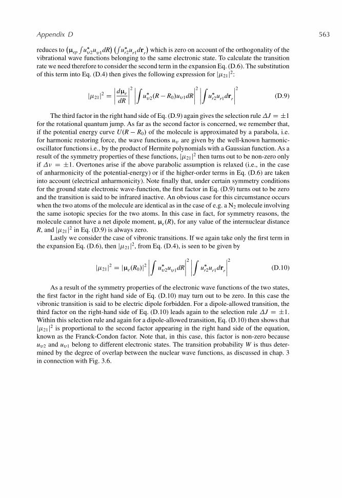
Appendix D 563
reduces toμep
Ru�
�2u�1dR
� Ru�
r2ur1drr
�which is zero on account of the orthogonality of the
vibrational wave functions belonging to the same electronic state. To calculate the transitionrate we need therefore to consider the second term in the expansion Eq. (D.6). The substitutionof this term into Eq. (D.4) then gives the following expression for j�21j2:
j�21j2 Dˇˇdμe
dR
ˇˇ2ˇˇZ u�
�2.R � R0/u�1dR
ˇˇ2ˇˇZ u�
r2ur1drr
ˇˇ2 (D.9)
The third factor in the right hand side of Eq. (D.9) again gives the selection ruleJ D ˙1for the rotational quantum jump. As far as the second factor is concerned, we remember that,if the potential energy curve U.R � R0/ of the molecule is approximated by a parabola, i.e.for harmonic restoring force, the wave functions u� are given by the well-known harmonic-oscillator functions i.e., by the product of Hermite polynomials with a Gaussian function. As aresult of the symmetry properties of these functions, j�21j2 then turns out to be non-zero onlyif � D ˙1. Overtones arise if the above parabolic assumption is relaxed (i.e., in the caseof anharmonicity of the potential-energy) or if the higher-order terms in Eq. (D.6) are takeninto account (electrical anharmonicity). Note finally that, under certain symmetry conditionsfor the ground state electronic wave-function, the first factor in Eq. (D.9) turns out to be zeroand the transition is said to be infrared inactive. An obvious case for this circumstance occurswhen the two atoms of the molecule are identical as in the case of e.g. a N2 molecule involvingthe same isotopic species for the two atoms. In this case in fact, for symmetry reasons, themolecule cannot have a net dipole moment, μe.R/, for any value of the internuclear distanceR, and j�21j2 in Eq. (D.9) is always zero.
Lastly we consider the case of vibronic transitions. If we again take only the first term inthe expansion Eq. (D.6), then j�21j2, from Eq. (D.4), is seen to be given by
j�21j2 D jμe.R0/j2
ˇˇZ u�
�2u�1dR
ˇˇ2ˇˇZ u�
r2ur1drr
ˇˇ2 (D.10)
As a result of the symmetry properties of the electronic wave functions of the two states,the first factor in the right hand side of Eq. (D.10) may turn out to be zero. In this case thevibronic transition is said to be electric dipole forbidden. For a dipole-allowed transition, thethird factor on the right-hand side of Eq. (D.10) leads again to the selection rule J D ˙1.Within this selection rule and again for a dipole-allowed transition, Eq. (D.10) then shows thatj�21j2 is proportional to the second factor appearing in the right hand side of the equation,known as the Franck-Condon factor. Note that, in this case, this factor is non-zero becauseu�2 and u�1 belong to different electronic states. The transition probability W is thus deter-mined by the degree of overlap between the nuclear wave functions, as discussed in chap. 3in connection with Fig. 3.6.
E
Space Dependent Rate Equations
The purpose of this appendix is to develop a rate-equation treatment, and to solve these equa-tions for the c.w. case, when the spatial variation of both the pump-rate and the cavity field aretaken into account. As a result of these spatial variations, the population inversion will also bespace dependent. In all cases, we will assume the laser oscillating on a single mode.
E.1. FOUR-LEVEL LASER
For an ideal four-level laser, we can neglect the population, N1, of the lower laser leveland thus let N Š N2 represent the population inversion. We can then write
@N
@ tD Rp � WN � N
�(E.1.1a)
d�
dtDZa
WNdV � �
�c(E.1.1b)
where the integral in Eq. (E.1.1b) is taken over the volume of the active medium and where themeaning of all other symbols has already been given in Chap. 7. Equation (E.1.1a) expressesa local balance between pumping, stimulated emission, and spontaneous decay processes.Note that a partial derivative has been used on the left-hand side of the equation on accountof the expected spatial variation of N. The integral term on the right-hand side of Eq. (E.1.1b)accounts for the contribution of stimulated processes to the total number of cavity photons �.This term has been written on the basis of a simple balance, using the fact that each individualstimulated process produces a photon. For a plane wave, we can now write W D �F D �I=h�and I D c�=n, where � is the stimulated-emission cross-section, F is photon flux, I is theintensity of the wave, � is the energy density in the active medium and n is its refractive index.
565
566 Appendixes
From the previous expressions, we can then relate W to the energy density of the wave as
W D c�
nh�� (E.1.2)
Although this equation has been derived, for simplicity, for a plane wave, one immedi-ately recognizes that it merely establishes a local relation between the transition rate and theenergy density of the e.m. field. It then follows that this equation has a general validity andcan thus represent the relation between W and � for e.g. the e.m. field of the cavity. In this case� is expected to be dependent on both space, r, and, for a transient case, also on time, t, thespatial dependence accounting for the spatial variation of the cavity mode. Equations (E.1.1),with the help of Eq. (E.1.2) give
@N
@ tD Rp � c�
nh��N � N
�(E.1.3a)
d�
dtD c�
nh�
Za
�NdV � �
�c(E.1.3b)
Note that, since both Rp and � are assumed to depend on position (and time for a tran-sient case), this will also apply to N, which cannot therefore be taken out of the integral inEq. (E.1.3b). Note also that the total number of cavity photons � may be related to the energydensity of the e.m. wave by
� D 1
h�
Zc
� dV (E.1.4)
where the integral is taken over the whole volume of the cavity. We will consider a lasercavity of length L in which is inserted an active medium of length l and refractive index n andwe will assume that the beam waist is located somewhere in the active medium. Under theseconditions, the energy density of the mode outside, �out, and inside, �in, the active mediumcan be written, respectively, as
�out D �0ju.r/j2 (E.1.5a)
�in D n�0ju.r/j2 (E.1.5b)
where u.r/ is the field amplitude, at the general coordinate, r, normalized to its peak value(occurring at the waist), and n�0 is the energy density at the waist location. From Eqs. (E.1.4)and (E.1.5) we then obtain
� D �0
h�
0@n
Za
juj2dV CZr
juj2dV
1A (E.1.6)
where the two integrals are taken over the active medium and the remaining volume of thecavity, respectively. The form of Eq. (E.1.6) suggests that we define an effective volume of
Appendix E 567
the mode in the cavity, V , as
V D0@n
Za
juj2dV CZr
juj2dV
1A (E.1.7)
and a volume Va of the mode in the active medium as
Va DZa
juj2dV (E.1.8)
With the help of Eqs. (E.1.5b), (E.1.6), and (E.1.7), Eq. (E.1.3) transform to
@N
@ tD Rp � c�
V� Njuj2 � N
�(E.1.9a)
d�
dtD24c�
V
Za
Njuj2dV � 1
�c
35 � (E.1.9b)
which represents our final result describing the space dependent rate equations of a four-level laser.
We will now solve Eq. (E.1.9) for the case of a c.w. laser oscillating on a single TEM00
mode. For simplicity, we will further assume the e.m. cavity field, u.r/, to be independent ofthe longitudinal coordinate z. This implies that we are neglecting both the spot size variationand the mode standing-wave-pattern along the laser cavity. We will also take the cladded-rodmodel discussed in Sect. 6.3.3. so that one needs not to worry about the aperturing effectcaused by a finite rod-diameter. Under these assumptions we can write the following verysimple expression for ju.r/j, holding for any value of the longitudinal coordinate z in theactive medium, and for any value of the radial coordinate, r, between 0 and 1:
juj D exp �.r =w0/2 (E.1.10)
where w0 is the spot size at the beam waist. Equation (E.1.7) then gives
V D w20
2Le (E.1.11)
where the equivalent length of the cavity, Le, can be expressed as [see Eq. (7.2.11)]
Le D L C .n � 1/l (E.1.12)
Likewise, from Eq. (E.1.8), we obtain
Va D w20
2l (E.1.13)
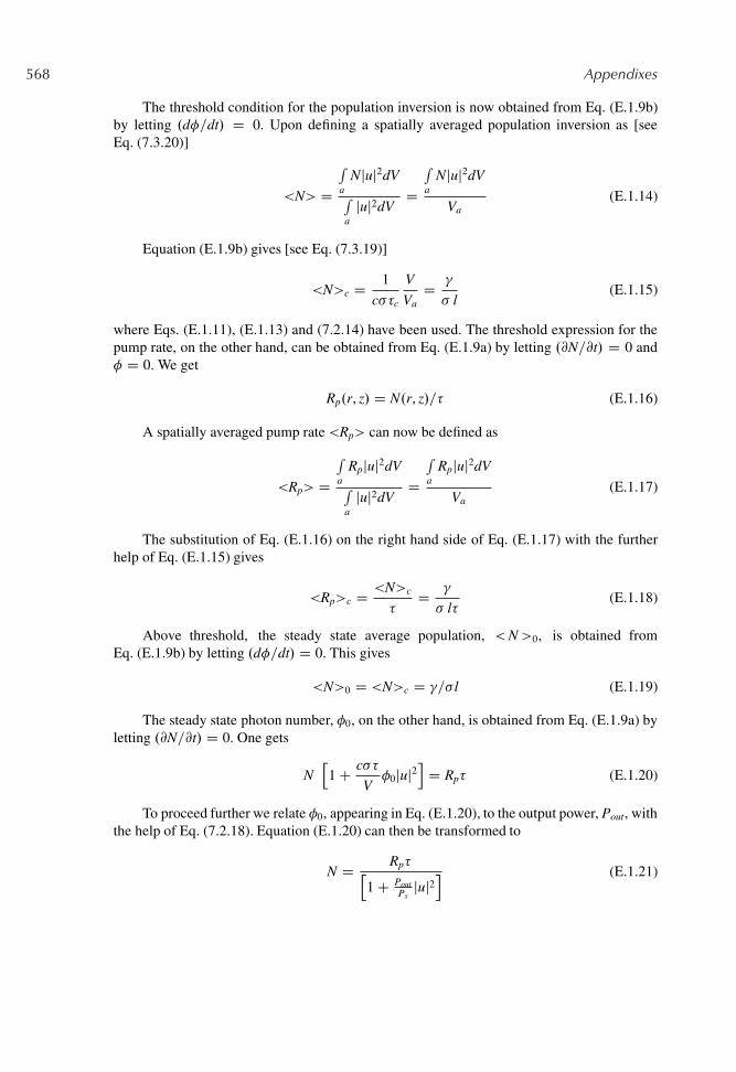
568 Appendixes
The threshold condition for the population inversion is now obtained from Eq. (E.1.9b)by letting .d�=dt/ D 0. Upon defining a spatially averaged population inversion as [seeEq. (7.3.20)]
<N> DRa
Njuj2dVRa
juj2dVDRa
Njuj2dV
Va(E.1.14)
Equation (E.1.9b) gives [see Eq. (7.3.19)]
<N>c D 1
c��c
V
VaD �
� l(E.1.15)
where Eqs. (E.1.11), (E.1.13) and (7.2.14) have been used. The threshold expression for thepump rate, on the other hand, can be obtained from Eq. (E.1.9a) by letting .@N=@t/ D 0 and� D 0. We get
Rp.r, z/ D N.r, z/=� (E.1.16)
A spatially averaged pump rate <Rp> can now be defined as
<Rp> DRa
Rpjuj2dVRa
juj2dVDRa
Rpjuj2dV
Va(E.1.17)
The substitution of Eq. (E.1.16) on the right hand side of Eq. (E.1.17) with the furtherhelp of Eq. (E.1.15) gives
<Rp>c D <N>c
�D �
� l�(E.1.18)
Above threshold, the steady state average population, <N>0, is obtained fromEq. (E.1.9b) by letting .d�=dt/ D 0. This gives
<N>0 D <N>c D �=� l (E.1.19)
The steady state photon number, �0, on the other hand, is obtained from Eq. (E.1.9a) byletting .@N=@t/ D 0. One gets
Nh1 C c��
V�0juj2
iD Rp� (E.1.20)
To proceed further we relate �0, appearing in Eq. (E.1.20), to the output power, Pout, withthe help of Eq. (7.2.18). Equation (E.1.20) can then be transformed to
N D Rp�h1 C Pout
Psjuj2
i (E.1.21)
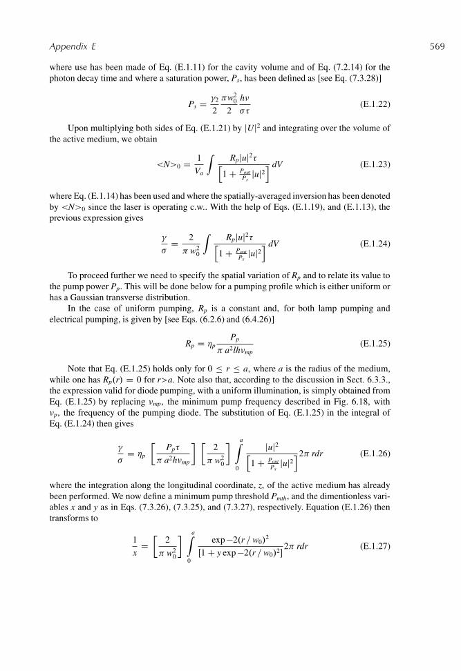
Appendix E 569
where use has been made of Eq. (E.1.11) for the cavity volume and of Eq. (7.2.14) for thephoton decay time and where a saturation power, Ps, has been defined as [see Eq. (7.3.28)]
Ps D �2
2
w20
2
h�
��(E.1.22)
Upon multiplying both sides of Eq. (E.1.21) by jUj2 and integrating over the volume ofthe active medium, we obtain
<N>0 D 1
Va
ZRpjuj2�h
1 C PoutPs
juj2i dV (E.1.23)
where Eq. (E.1.14) has been used and where the spatially-averaged inversion has been denotedby <N>0 since the laser is operating c.w.. With the help of Eqs. (E.1.19), and (E.1.13), theprevious expression gives
�
�D 2
w20
ZRpjuj2�h
1 C PoutPs
juj2i dV (E.1.24)
To proceed further we need to specify the spatial variation of Rp and to relate its value tothe pump power Pp. This will be done below for a pumping profile which is either uniform orhas a Gaussian transverse distribution.
In the case of uniform pumping, Rp is a constant and, for both lamp pumping andelectrical pumping, is given by [see Eqs. (6.2.6) and (6.4.26)]
Rp D �pPp
a2lh�mp(E.1.25)
Note that Eq. (E.1.25) holds only for 0 r a, where a is the radius of the medium,while one has Rp.r/ D 0 for r>a. Note also that, according to the discussion in Sect. 6.3.3.,the expression valid for diode pumping, with a uniform illumination, is simply obtained fromEq. (E.1.25) by replacing �mp, the minimum pump frequency described in Fig. 6.18, with�p, the frequency of the pumping diode. The substitution of Eq. (E.1.25) in the integral ofEq. (E.1.24) then gives
�
�D �p
�Pp�
a2h�mp
� �2
w20
� aZ0
juj2h1 C Pout
Psjuj2
i2 rdr (E.1.26)
where the integration along the longitudinal coordinate, z, of the active medium has alreadybeen performed. We now define a minimum pump threshold Pmth, and the dimentionless vari-ables x and y as in Eqs. (7.3.26), (7.3.25), and (7.3.27), respectively. Equation (E.1.26) thentransforms to
1
xD�
2
w20
� aZ0
exp �2.r =w0/2
Œ1 C y exp �2.r =w0/2�2 rdr (E.1.27)
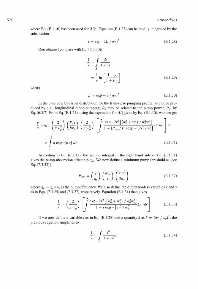
570 Appendixes
where Eq. (E.1.10) has been used for jUj2. Equation (E.1.27) can be readily integrated by thesubstitution
t D exp �2.r =w0/2 (E.1.28)
One obtains [compare with Eq. (7.3.30)]
1
xD
1Zˇ
dt
1 C yt
D 1
yln
�1 C y
1 C ˇ y
�(E.1.29)
where
ˇ D exp �.a =w0/2 (E.1.30)
In the case of a Gaussian distribution for the transverse pumping profile, as can be pro-duced by e.g., longitudinal diode-pumping, Rp may be related to the pump power, Pp, byEq. (6.3.7). From Eq. (E.1.24), using the expression for jUj given by Eq. (E.1.10), we then get
�
�D�r�t
2
w2p
! �Pp�
h�p
� �2
w20
� 24
1Z0
exp �2r2�
w20 C w2
p
�=w2
0w2p
1 C .Pout =Ps/ exp � �2r2 =w2
0
2 rdr
35 �
�lZ
0
˛ exp �Œ˛ z� dz (E.1.31)
According to Eq. (6.3.11), the second integral in the right hand side of Eq. (E.1.31)gives the pump-absorption efficiency �a. We now define a minimum pump threshold as [seeEq. (7.3.32)]
Pmth D��
�p
� �h�p
�
� w2
p
2�e
!(E.1.32)
where �p D �r�t�a is the pump efficiency. We also define the dimensionless variables x and yas in Eqs. (7.3.25) and (7.3.27), respectively. Equation (E.1.31) then gives
1
xD�
2
w20
� 24
1Z0
exp �2r2�
w20 C w2
p
�=w2
0w2p
1 C y exp � �2r2 =w2
0
2 rdr
35 (E.1.33)
If we now define a variable t as in Eq. (E.1.28) and a quantity ı as ı D .w0 =wp/2, the
previous equation simplifies to
1
xD
1Z0
tı
1 C yıdt (E.1.34)
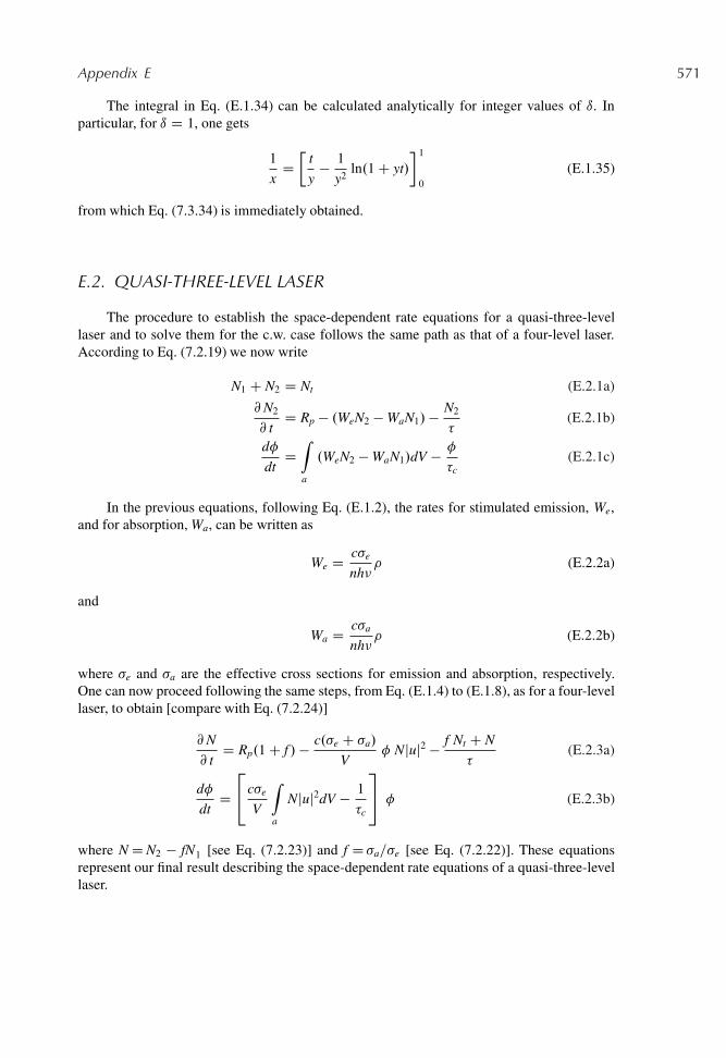
Appendix E 571
The integral in Eq. (E.1.34) can be calculated analytically for integer values of ı. Inparticular, for ı D 1, one gets
1
xD�
t
y� 1
y2ln.1 C yt/
� 1
0(E.1.35)
from which Eq. (7.3.34) is immediately obtained.
E.2. QUASI-THREE-LEVEL LASER
The procedure to establish the space-dependent rate equations for a quasi-three-levellaser and to solve them for the c.w. case follows the same path as that of a four-level laser.According to Eq. (7.2.19) we now write
N1 C N2 D Nt (E.2.1a)
@N2
@ tD Rp � .WeN2 � WaN1/� N2
�(E.2.1b)
d�
dtDZa
.WeN2 � WaN1/dV � �
�c(E.2.1c)
In the previous equations, following Eq. (E.1.2), the rates for stimulated emission, We,and for absorption, Wa, can be written as
We D c�e
nh�� (E.2.2a)
and
Wa D c�a
nh�� (E.2.2b)
where �e and �a are the effective cross sections for emission and absorption, respectively.One can now proceed following the same steps, from Eq. (E.1.4) to (E.1.8), as for a four-levellaser, to obtain [compare with Eq. (7.2.24)]
@N
@ tD Rp.1 C f / � c.�e C �a/
V� Njuj2 � f Nt C N
�(E.2.3a)
d�
dtD24c�e
V
Za
Njuj2dV � 1
�c
35 � (E.2.3b)
where N D N2 � fN1 [see Eq. (7.2.23)] and f D �a=�e [see Eq. (7.2.22)]. These equationsrepresent our final result describing the space-dependent rate equations of a quasi-three-levellaser.
572 Appendixes
We will now solve Eq. (E.2.3) for the case of a c.w. laser oscillating on a single TEM00
mode. Under the assumption, again, that ju.r/j is described by Eq. (E.1.10) for 0<r<1, weobtain again Eqs. (E.1.11), (E.1.12) and (E.1.13) for V , Le, and Va, respectively. We alsodefine the spatially averaged values, <N>, and, <Rp>, as in Eqs. (E.1.14) and (E.1.17),respectively.
The threshold value of <N> is obtained from Eq. (E.2.3b) by letting .d�=dt/ D 0.This gives
<N>c D �=�el (E.2.4)
The threshold value of <Rp> is then obtained from Eq. (E.2.3a) by letting .@N=@t/ D 0and � D 0. One gets
<Rp>c D f<Nt>C<N>c
.1 C f /�D �a<Nt>l C �
.�e C �a/l�(E.2.5)
Above threshold, the steady state value, <N>0, is again obtained from Eq. (E.2.3b) byletting .d�=dt/ D 0. One gets
<N>0 D <N>c D �=�el (E.2.6)
From Eq. (E.2.3a), under the condition .@N=@t/ D 0, one obtains
N D Rp.1 C f /� � f Nt
1 C Œc.�e C �a/�=V��0juj2(E.2.7)
and the steady-state number of photons, �0, can again be related to the output power, Pout, byEq. (7.2.18). Equation (E.2.7) can then be transformed to
N D Rp.1 C f /� � f Nt
1 C yjuj2 (E.2.8)
In the previous expression we have again defined y D Pout=Ps, where the saturationpower, Ps, is now given by
Ps D �2
2
w20
2
h�
.�e C �a/�(E.2.9)
We now multiply both sides of Eq. (E.2.8) by jUj2 and integrate over the volume of theactive medium. With the help of Eqs. (E.1.13), (E.1.14) and (E.2.6) we obtain [compare withEq. (E.1.24)]
�
�D 2
w20
ZŒRp.1 C f /� � f Nt�juj2
Œ1 C yjuj2� dV (E.2.10)
Appendix E 573
To proceed further, the spatial dependence of Rp needs to be specified. In the case oflongitudinal pumping with a pump beam of Gaussian radial profile we use Eq. (6.3.7). Withthe help of Eq. (E.1.10) for juj, Eq. (E.2.10) can be written as
�
�elD �r�t.1 C f /
�Pp�
h�p
� 2
w2pl
! 1Z0
tı
1 C ytdt
lZ0
˛ exp �.˛z/dz�
� f Nt
1Zˇ
dt
1 C yt(E.2.11)
where t and ˇ are expressed by Eqs. (E.1.28) and (E.1.30), respectively, and
ı D .w0 =wp/2 (E.2.12)
Again recognizing that the integral over the longitudinal coordinate z is the absorptionefficiency �a, and under the simplifying assumption w0<<a (i.e. ˇ Š 0), Eq. (E.2.11) gives
� D �p.�e C �a/
�Pp�
h�p
� 2
w2p
! 1Z0
tı
1 C ytdt � �aNtl
ln.1 C y/
y(E.2.13)
and this equation can be solved for Pp to get
Pp D �
�h�p
�p�
� " w2
p
2.�e C �a/
#1
1R0Œtıı
1 C yt� dt
�1 C B
ln.1 C y/
y
�(E.2.14)
where B D �aNtl=� . The minimum pump threshold is obtained from Eq. (6.3.25) whenw0<<wp and �aNtl<<� . One obtains [see Eq. (7.4.16)]
Pmth D �
�h�p
�p�
� " w2
p
2.�e C �a/
#(E.2.15)
By taking the ratio between Eqs. (E.2.14) and (E.2.15) we obtain our final result [seeEq. (7.4.18)]
x D 11R
0
tı
1Cyt dt
�1 C B
ln.1 C y/
y
�(E.2.16)
F
Theory of Mode-Locking:Homogeneous Line
According to the discussion presented in Sect. 8.6.3, a theory of mode-locking can bedeveloped, in the time domain, by requiring that the pulse reproduce itself after each cav-ity round trip. We will limit our discussion here to the case of a homogeneous line and we willfurther assume that the lifetime of the upper laser level is much longer than the cavity round-trip time. Under these conditions, the saturated single-pass power gain of the amplifier, at thetransition peak, is given by g0 D �pN0l, where �p is the peak cross-section, l is the length ofthe active medium and N0 is the steady-state inversion, as established by the cumulative effectof the passage of many pulses. This means that this saturated gain will be determined by theaverage intracavity beam intensity<I> and can thus be related to the unsaturated gain, g, by
g0 D g
1 C .< I > =Is/(F.1)
where Is D h�0=�p� is the saturation intensity of the amplifier, at the transition peak.
F.1. ACTIVE MODE-LOCKING
This theory was developed by Kuizenga and Siegman.1/ and, later on, put in a moregeneral framework by Haus [2,3]. We will follow the latter treatment and for brevity we willlimit our considerations to mode-locking by an amplitude modulator. Thus, we consider thelaser configuration of Fig. F1 and assume that the modulator is very thin and placed as nearas possible to mirror 2. Under these conditions, a single light pulse is expected to be travelingback and forth within the cavity (see Fig. 8.19). At any given position within the cavity, the
575
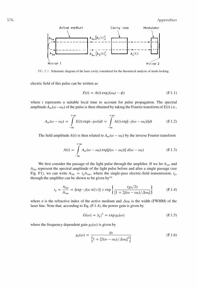
576 Appendixes
FIG. F.1. Schematic diagram of the laser cavity considered for the theoretical analysis of mode-locking.
electric field of this pulse can be written as
E.t/ D A.t/ exp j.!0t � �/ (F.1.1)
where t represents a suitable local time to account for pulse propagation. The spectralamplitude A!.!�!0/ of the pulse is then obtained by taking the Fourier transform of E.t/ i.e.,
A!.! � !0/ DC1Z
�1E.t/ exp.�j!t/dt D
C1Z�1
A.t/ expŒ�j.! � !0/t�dt (F.1.2)
The field amplitude A.t/ is then related to A!.! � !0/ by the inverse Fourier transform
A.t/ DC1Z
�1A!.! � !0/ expŒj.! � !0/t� d.! � !0/ (F.1.3)
We first consider the passage of the light pulse through the amplifier. If we let A1! andA2! represent the spectral amplitude of the light pulse before and after a single passage (seeFig. F1), we can write A2! D tgA1! , where the single-pass electric-field transmission, tg,through the amplifier can be shown to be given by.4/
tg D A2!
A1!
D Œexp �j.! nl=c/� � exp
.g0=2/
Œ1 C 2j.! � !0/=!0�
�(F.1.4)
where n is the refractive index of the active medium and !0 is the width (FWHM) of thelaser line. Note that, according to Eq. (F.1.4), the power gain is given by
G.!/ D jtgj2 D exp g0.!/ (F.1.5)
where the frequency dependent gain g0.!/ is given by
g0.!/ D g0n1 C Œ2.! � !0/=!0�
2o (F.1.6)
Appendix F 577
i.e., it shows the expected Lorentzian shape of a homogeneous line. If we assume that thespectral width of the light pulse is appreciably narrower than !0, the expression appearingas the argument of the second exponential function in Eq. (F.1.4) can be expanded as a powerseries in .! � !0/. To first order, this gives
tg D exp �j f.! nl=c/C Œg0.! � !0/=!0�g �� exp.g0=2/
˚1 � Œ2.! � !0/=!0�
2� (F.1.7)
The imaginary terms in the first exponential function correspond to a phase delay� D .!nl=c/ C Œg0.! � !0/=!0�, from which, according to Eq. (8.6.27), the time delay,�d, experienced by the pulse after traveling in the active medium is obtained as
�d D d�
d!D nl
cC g0
!0(F.1.8)
Note that this delay is not simply nl=c because the gain line gives an additional finitecontribution. This delay should be taken into account when considering the requirement thatthe round-trip pulse propagation time be set equal to the period of the amplitude modulator.For simplicity we will not consider any further the effect of this delay as well as that of allother cavity elements, the pulse amplitude being referred, in any case, to a local time wherethese delays are taken into account. We therefore ignore the phase term in Eq. (F.1.7) and write
tg D exp˚.g0=2/
˚1 � Œ2.! � !0/=!0�
2��
(F.1.9)
We also ignore the loss introduced by mirror 1, since this will be taken into accountin the overall cavity loss. After passing once more through the active medium, thespectral amplitude of the light pulse will experience another transmission factor ta asgiven by Eq. (F.1.9). The round trip transmission through the amplifier is then given byt2g D .A3!=A1!/ D exp
˚g0˚1 � Œ2.! � !0/=!0�
2��
, where A3! is the spectral amplitude ofthe light pulse after one round trip through the amplifier. Under the assumption g0 � 1, thislast equation gives
A3! D t2gA1! D A1!
1 C g0
˚1 � Œ2.! � !0/=!0�
2�� (F.1.10)
To proceed further we need to calculate the effect of this transmission in the time-domainrather than in the frequency-domain. For this we note the following property of a Fouriertransform .F.T./:
F.T.
�dnA.t/
dtn
�D Œj.! � !0/�
n A!.! � !0/ (F.1.11)
This relation can be readily proved by taking first the n-th derivative and then the Fouriertransform of both sides of Eq. (F.1.3). Equation (F.1.11) shows that the multiplication of thespectral amplitude A! by k.! �!0/
n, where k is a constant, is equivalent, in the time domain,of taking .k=jn/ times the n-th derivative of the amplitude A.t/. We can apply this rule to eachindividual term on the right hand side of Eq. (F.1.10) to obtain
A3.t/ D(
1 C g0
"1 C
�2
!0
�2 d2
dt2
#)A1.t/ (F.1.12)
578 Appendixes
where A1.t/ and A3.t/ are, respectively, the amplitudes of the light pulse entering the amplifierand after one round trip (see Fig. F1). Equation (F.1.12) shows that the effect on the light pulseamplitude of a round trip passage through the gain medium, can be described by a round-tripoperator
OTg D(
1 C g0
"1 C
�2
!0
�2 d2
dt2
#)(F.1.13)
We next consider the effect of cavity losses arising from finite mirror reflectivities andinternal losses. These losses are represented by the central box in Fig. F1. If we then let � bethe logarithmic power loss per pass, we can write, for a single passage in the cavity,
A4.t/ D Œexp.��=2/�A3.t/ (F.1.14)
In fact, according to Eq. (F.1.14), the ratio of corresponding intensities .I4=I3/ D.A4=A3/
2 indeed shows the expected value exp.��/. From Eq. (F.1.14) one finds that thetransmission accounting for the round trip losses is given by exp.��/ and this expression, for� � 1, can be approximated by 1 � � . This means that the operator corresponding to theround trip loss in the cavity is simply
OTl D 1 � � (F.1.15)
Lastly, we consider the effect of the amplitude modulator. We let �mŒ1 � cos!mt�, rep-resent the single-pass logarithmic power-loss introduced by the modulator. In this expression!m is the modulator frequency which is assumed to be such that the modulator period is equalto the round trip time of the light pulse in the laser cavity. The single pass transmission of thefield amplitude through the modulator will then be given by
tm D exp f � .�m=2/Œ1 � cos!mt�g (F.1.16)
The transmission for a double pass through the modulator is then t2m D exp f � .�m/
Œ1 � cos!mt�g and this expression, for �m � 1, can be approximated to t2m Š 1 � .�m/
Œ1�cos!mt�. We now assume that the pulse passes through the modulator when the modulator-loss is zero (see Fig. 8.20), i.e. at time t D 0, and that the pulsewidth is much smaller that themodulator period 2 =!m. Under these conditions, the round trip transmission can be furtherapproximated to t2
m D 1 � .�m=2/.!mt/2. The operator corresponding to a double-passage ofthe pulse through the modulator is then simply given by
OTm D 1 � �m
2.!mt/2 (F.1.17)
Having established the operators which describe the time-domain evolution of the pulseupon a double passage through the three components considered, we now require that, in thesteady state regime, the pulse amplitude A.t/ reproduces itself after a round trip. We thus write
OTm OTl OTg A.t/ D A.t/ (F.1.18)
Appendix F 579
Using the previous expressions for OTm, OTl, and OTg and again using the condition thatŒg0, � , �m� � 1 we obtain the following differential equation
(g0
"1 C
�2
!0
�2 d2
dt2
#� � � �m
2!2
m t2
)A.t/ D 0 (F.1.19)
which is the final result of our calculation. This equation is readily seen to be equivalent tothe Schrodinger equation for a particle in a parabolic potential (harmonic oscillator), whosesolution is well known. The solution, in our case, can then be written as
A.t/ D Hn.!pt/ exp � !2
p t2
2
!(F.1.20)
where Hn is the Hermite polynomial of order n, and where
!p D��m
2g0
� 1=4 �!m!0
2
� 1=2
(F.1.21)
and
1 � �
g0D 4!2
p
!20
.2n C 1/ (F.1.22)
It can also be shown, however, that, out of all these solutions, only the first orderGaussian solution .n D 0/ is stable.
Equations (F.1.21) and (F.1.22) represent a set of two relations for the unknown param-eters !p and g0. From a knowledge of !p one then gets the width of the mode-lockedpulse. The full width at half maximum intensity of the pulse, �p, is in fact given by�p D 2 Œln 2�1=2 =!p and from Eq. (F.1.21) one gets
�p D"
2p
2 ln 2
2
# 1=2 �g0
�m
� 1=4 � 1
�m�0
� 1=2
(F.1.23)
where �m D !m=2 and �0 D !0=2 . We note that the first factor on the right hand sideof Eq. (F.1.23) is approximately equal to 0.45 while the second factor, as a result of the 1/4thpower, is approximately equal to unity. The values of�p and, hence, !p are then only weaklydependent on g0 and from Eq. (F.1.23) one obtains the following approximate expression for�p [see Eq. (8.6.19)]:�p Š 0.45=.�m�0/
1=2. From Eq. (F.1.22), with n D 0, the value ofg0 can now be obtained. Note that, according to Eq. (F.1.22), g0 turns out to be larger than� on account of the presence of the modulator loss. Once the value of g0 is calculated, theaverage intracavity laser intensity,< I >, is obtained from (F.1) since one has g D �pNl D x�where x D N=Nc D Rp=Rpc is the amount by which threshold is exceeded. Knowing theaverage intracavity laser intensity, the laser pulse duration and the pulse repetition rate, onethen obtains the laser peak intensity.
580 Appendixes
F.2. PASSIVE MODE-LOCKING
We will consider the theory of passive mode-locking by a saturable absorber with alifetime much shorter than the pulse duration (fast saturable absorber)..5/ We will again referto Fig. F1, where the modulator is now replaced by this fast absorber.
According to Eq. (F.1.13), the effect on the pulse amplitude due to a round-trip passagethrough the gain medium can be described by the operator
OTg D(
1 C g00
"1 C
�2
!0
�2 d2
dt2
#)(F.2.1)
where, to conform with the discussion presented in Sect. 8.6.3.2., the saturated gain has beendenoted by g0
0. According to Eq. (F.1.15), the effect of the unsaturable cavity losses, can bedescribed by
OTl D 1 � �c (F.2.2)
where �c is the cavity loss without the saturable absorber. According to Eq. (F.1.14), thesingle-pass amplitude-transmission of the saturable absorber is then written as
tsa D exp �.�sa=2/ (F.2.3)
In the previous expression �sa represents the, saturated, single-pass power-loss of theabsorber and is given by
�sa D � 0
1 C .I=Is/(F.2.4)
where � 0 is the unsaturated loss, I D I.t/ is the pulse intensity, and Is is the saturation inten-sity of the absorber. The amplitude-transmission for a double passage through the saturableabsorber is then given by t2
sa D exp �.�sa/ and, under the assumptions � 0 � 1 and .I=Is/ � 1,this last equation, with the help of Eq. (F.2.4) gives t2
sa Š 1 � �sa Š 1 � � 0Œ1 � .I=Is/� D1�� 0Œ1�.jAj2=Is/�, where the amplitude A.t/ is now normalized so that jAj2 is the beam inten-sity. From the previous expression for t2
sa we obtain the operator corresponding to a doublepass through the saturable absorber as
OTsa D 1 � � 0 C � 0 jAj2
Is(F.2.5)
Self-consistency now requires that
OTm OTl OTsaA.t/ D A.t/ (F.2.6)
From Eqs. (F.2.1), (F.2.2) and (F.2.5), again assuming Œg00, � , � 0� � 1, we get
(g0
0
"1 C
�2
!0
�2 d2
dt2
#� �c � � 0 C � 0 jAj2
Is
)A.t/ D 0 (F.2.7)
Appendix F 581
The solution of Eq. (F.2.7) can be written as
A.t/ D A0
cosh .t=�p/(F.2.8)
where
�p D�
2g00
� 0
� 1=2 � 2
!0
� �Is
jA0j2
� 1=2
(F.2.9)
and
�c C � 0 � g00 D 4g0
0
!20�
2p
(F.2.10)
Since the width of the pulse intensity, �p, (FWHM) is given by �p D 1.76 �p and!0 D 2 �0, from Eq. (F.2.9) one obtains Eq. (8.6.22) by recognizing that jA0j2 is thepeak laser intensity. Equation (F.2.10), on the other hand, shows that g0
0 < �c C� 0 D � , where� is the overall unsaturated loss of the cavity. This means that, in the absence of the pulse, thelaser has a net loss while a net gain only exists during the passage of the mode-locked pulse(see Fig. 8.22).
References
1. D. J. Kuizenga and A. E. Siegman, FM and AM Mode Locking of the Homogeneous Laser- Part I: Theory, IEEEJ. Quantum Electron., QE-6, 694–708 (1970).
2. H. A. Haus, A Theory of Forced Mode-Locking, IEEE J. Quantum Electron., QE-11, 323–330 (1975).3. H. A. Haus, Waves and Fields in Optoelectronics, Prentice Hall, Inc., Englewoods Clifts, 1984, Section 9.3.4. A. E. Siegman, Lasers (Oxford University Press, Oxford, 1986) Sec. 7.4.5. H. A. Haus, Theory of Mode-Locking with a Fast Saturable Absorber, J. Appl. Phys., 46, 3049–3058 (1975).
G
Propagation of a Laser Pulse Througha Dispersive Medium or a GainMedium
Consider first a light pulse traveling in a dispersive medium, and let !L and !L be, respec-tively, the center frequency and the width of the corresponding spectrum (Fig. 8.25a). Theelectric field, E.t, z/, of the corresponding waveform, at coordinate z along the propagationdirection, can generally be expressed in terms of a Fourier expansion as
E.t, z/ DC1Z
�1A!.! � !L/ expŒj.!t � ˇz/�d! (G.1)
where A! D A!.! � !L/ is the complex amplitude of each field component and ˇ D ˇ.!�!L/ describes the dispersion relation of the medium.
Let us now assume that the dispersion relation of the medium, over the bandwidth!L,can be approximated by a linear relation, i.e.,
ˇ D ˇL C�
dˇ
d!
�!L
.! � !L/ (G.2)
where ˇL is the propagation constant corresponding to the frequency !L. On substitutingEq. (G.2) in Eq. (G.1) one can see that this last equation can be written as
E.t, z/ D expŒj.!Lt � ˇLz/� �C1Z
�1A!.!/ exp
(j!
"t �
�dˇ
d!
�!L
z
#)d! (G.3)
where ! D ! � !L. From Eq. (G.3) we can now see that the integration over ! leadsto a function of the single variable Œt � .dˇ=d!/!L z�. Equation (G.3) can therefore be put in
583
584 Appendixes
the form
E.t, z/ D AŒt � .z=�g/� expŒj.!Lt � ˇLz/� (G.4)
where A is the pulse amplitude, expŒj.!Lt � ˇLz/� is the carrier wave, and �g is given by
�g D�
d!
dˇ
�ˇDˇL
(G.5)
The fact that the pulse amplitude is a function of the variable t � .z=�g/ means that the pulsepropagates without changing its shape and at a speed �g. This velocity is called the groupvelocity of the pulse and, according to Eq. (G.5), is given by the slope of the ! vs ˇ relationat ! D !L (i.e. �g D tan 0, see Fig. 8.25a).
Consider next the case of a light pulse with a bandwidth!L so large that it is no longera good approximation to describe the dispersion relation by a linear law (Fig. 8.25c). In thiscase, different spectral regions of the pulse will travel with different group velocities and,consequently, the pulse will broaden as it propagates. After traversing the length l of themedium, the broadening of the pulse,�d, will then be given approximately by the differencein group delay between the slowest and the fastest spectral components, respectively. We canthen write
�d D
l
� 0g
� l
� 00g
!D l
��dˇ
d!
�!0
��
dˇ
d!
�!00
�(G.6)
where � 0g and � 00
g are the two group velocities of these components and !0 and !00 are the cor-responding frequencies. Let us now assume that the dispersion relation, within the bandwidth!L, can be approximated by a parabolic (or quadratic) law, i.e.,
ˇ D ˇL C�
dˇ
d!
�!L
.! � !L/C 1
2
�d2ˇ
d!2
�!L
.! � !L/2 (G.7)
From Eqs. (G.6) and (G.7) one gets
�d Š l
ˇˇ� d2ˇ
d!2
�!L
ˇˇ !L D j�00.!L/j !L (G.8)
where we have defined � D ˇl, �00 D d2�=d!2 and �00 is taken at the central laser fre-quency !L. Given the form of Eq. (G.8), the quantity �00.!L/, is referred to as the group delaydispersion (GDD) while the quantity
.d2ˇ=d!2/!L D GVD D Œd.1=�g/=d!�!L (G.9)
is referred to as the group velocity dispersion (GVD) at frequency !L.The calculation leading to Eq. (G.8) is open to criticism because, to obtain Eq. (G.8),
we have in fact been considering the propagation of limited spectral components of the pulse,each of which actually correspond to a different, and in fact, longer pulse than the original
Appendix G 585
one. A more precise and instructive calculation can be performed by assuming that the pulse,upon entering the medium at coordinate z D 0, has a Gaussian amplitude profile i.e.,
E.t/ D A0 exp � t2=2�2p
�exp.j!Lt/ (G.10)
where �p is the 1/e half-width of the pulse intensity. Since the spectral amplitude, A!.!�!L/,is a Gaussian function of .! � !L/, the electric field after a distance z in the medium can beeasily calculated from Eq. (G.1) if we assume that the dispersion relation can be developed ina Taylor expansion up to second order of .!�!L/, as shown in Eq. (G.7). In this case, in fact,the integrand in Eq. (G.1) can be readily expressed in terms of the inverse Fourier transformof a generalized Gaussian function of complex argument, whose integral is well known. Toshow the final result for the pulse amplitude, A(t, z), we refer to a new coordinate systemgiven by
t0 D t � .z=�g/ (G.11a)
z0 D z (G.11b)
�g being the group velocity. This means that the pulse amplitude is referred to a local timewhich takes into account the group delay of the pulse. Using this new coordinate system, thepulse amplitude turns out to be given by.1/
A.t0, z/ D A 0�p�2
p C jb2z�1=2
exp �"
.t0/2
2�2
p C jb2z�#
(G.12)
where, for simplicity, we have written b2 D .d2ˇ=d!2/!L D GVD, and where, on account ofEq. (G.11b), we have written, again for simplicity, z0 D z. According to Eq. (G.12), A.t0, z/then turns out to be given by a Gaussian function of t0 with complex argument so that wecan write
A.t0, z/ D jA.t0, z/j exp �j'.t0, z/ (G.13)
From Eq. (G.12), the pulse magnitude jA.t0, z/j can be readily calculated as
jA.t0, z/j D A0�p
Œ�4p C b2
2z2�1=4exp �
"t02�2
p
2.�4p C b2
2z2/
#(G.14)
Equation (G.14) shows that the Gaussian pulse maintains its shape on propagation and com-parison with Eq. (G.10) shows that the width of the pulse at coordinate z, �p.z/, is such that�2
p .z/ D �4
p C b22z2�=�2
p . This expression can then be transformed to
�p.z/ D �p
"1 C
�z
LD
�2#1=2
(G.15)
where LD D �2p =jb2j is called the dispersion length of the pulse in the medium. Note from
Eq. (G.15) the analogy of time-broadening of a Gaussian pulse in a dispersive medium and
586 Appendixes
spot-size increase of a Gaussian-beam due to diffraction [compare with Eq. (4.7.17a)], thedispersive length, in the former case, being the equivalent of the Rayleigh range in the lattercase. This analogy can be traced back to a formal analogy between the diffraction equation,in the paraxial approximation, and the differential equation describing pulse propagation in aquadratic dispersive medium..1/
From Eq. (G.12), the phase, '.t0, z/, can also be readily calculated as
'.t0, z/ D � sgn.b2/.z=LD/
1 C .z=LD/2t02
�2p
C 1
2tan�1
�z
LD
�(G.16)
where sgn.b2/ stands for the sign of b2 i.e., of GVD. Equation (G.16) shows that, '.t0, z/contains, besides the constant term .1=2/ tan�1.z=LD/, another term which is quadratic in t0.This means that the instantaneous frequency of the pulse, !.t0/ D @Œ.!Lt0/ � '.t0, z/�=@t0,given by
! D !L C sgn.b2/.z=LD/
1 C .z=LD/22t0
�2p
(G.17)
now has a term which changes linearly with time. Thus the pulse acquires a linear frequencychirp whose sign depends on the sign of b2. In particular, the instantaneous frequency willdecrease in time for a negative GVD.
If the length l of the medium is much smaller than the dispersion length, LD, the relativepulse broadening, .ı�p=�p/D D Œ�p.l/� �p�=�p, can be readily obtained from Eq. (G.15), as
�ı�p
�p
�D
Š 1
2
�l
LD
�2
D 1
2
�00
�2p
!2
(G.18)
where �00 D �00.!L/ D Œd2�=d!2�!L . The width of a Gaussian pulse intensity (FWHM) isthen related to the quantity �p appearing in Eq. (G.10) by�p D 2.ln 2/1=2�p. From Eq. (G.18)we then obtain �
ı�p
�p
�D
D .8 ln2 2/�002
�4p
(G.19)
Let us now consider a Gaussian pulse, as in Eq. (G.10), entering a homogeneously broadenedgain medium. The spectral amplitude of the pulse A!.! �!0/, while entering the medium, isobtained by taking the inverse Fourier transform of Eq. (G.10) and it is readily shown to begiven by
A!.! � !L/ / exp �".! � !L/
2�2p
2
#(G.20)
where !L is the central laser frequency. If the spectral width of the pulse is much smallerthan the gain linewidth, the gain for the electric field amplitude can be approximated as (seeAppendix F)
Ge.! � !0/ D expn�g0
2
� ˚1 � Œ2.! � !0/=�!0�
2�o (G.21)
Appendix G 587
where g0 D N0� l is the saturated single pass power gain through the amplifier and!0 is thelinewidth of the transition. The spectral amplitude of the pulse, after passing through the gainmedium, is then given by
Ag!.! � !0/ D Ge.! � !0/ � A!.! � !L/ (G.22)
From Eq. (G.22) with the help of Eqs. (G.20) and (G.21) and assuming !L D !0, we obtain
Ag!.! � !0/ / exp �(.! � !0/
2
"�2
p
2C g0
2
�2
!0
�2#)
(G.23)
Equation (G.23) shows that, within the approximation made, the spectrum remains Gaus-sian after the pulse has traversed the gain medium. A comparison of Eq. (G.23) withEq. (G.20) then indicates that the pulse duration has been broadened to a value � 0
p where� 02
p =2 corresponds to the term appearing in the square brackets of Eq. (G.23). We thus get
� 0p D �p
"1 C g0
�2
�p!0
�2#1=2
(G.24)
For small changes of pulse duration, the relative pulse broadening, .ı�p=�p/g D � 0
p � �p�=�p,
after the gain medium, is obtained from Eq. (G.24) as
�ı�p
�p
�g
D 1
2
�2
�p!0
�2
g0 (G.25)
Equation (G.25) can be readily recast in terms of the gain linewidth�0 D !0=2 and laserpulsewidth�p D 2.ln 2/1=2�p. We obtain
�ı�p
�p
�g
D�
2 ln 2
2
� 1
�2p�
20
!g0 (G.26)
References
1. Hermann A. Haus, Waves and Fields in Optoelectronics, Prentice Hall, Inc., Englewoods Clifts, 1984, Sect. 6.6
H
Higher-Order Coherence
The degree of coherence � .1/ introduced in Sect. 11.3 involves the first order correlationfunction < E.x1/E�.x2/ >, see Eq. (11.3.7), where, as a short-hand notation, the symbolxi D .ri, ti/ has been used to denote both space and time coordinates of the field. Likewisewe can define
� .n/.x1, x2, : : :, x2n/ D hE.x1/: : :E.xn/E�.xnC1/: : :E
�.x2n/i (H.1)
which involves the product of 2n terms, these being the functions E evaluated at the 2nspace-time points x1, x2, : : : , x2n. The corresponding normalized quantity, � .n/, can then bedefined as
� .n/.x1, x2, : : :, x2n/ D hE.x1/ : : :E.xn/E�.xnC1/ : : :E�.x2n/i2nQ1
rhE.xr/E�.xr/i1=2
(H.2)
whereQ
is the symbol for product. Obviously these expression reduce to Eqs. (11.3.7) and(11.3.8) for the case n D 1.
In terms of these higher-order correlation functions, we need now to define what wemean by a completely coherent beam. Thus, we begin by noting that, if a wave is perfectlycoherent to first order (i.e., if � .1/ .x1, x2/ D 1), then one must have
� .1/.x1, x2/ D E.x1/ E�.x2/ (H.3)
i.e., � .1/ must factorize into a product of the fields at x1 and x2. Indeed, if field fluctuationsare completely absent, the ensemble averages of e.g., Eq. (11.3.7) or (11.3.8) simply reduceto the product of the corresponding signals. By analogy one can define a perfectly coherente.m. wave as one for which � .n/ factorizes to all orders n. This means that
� .n/.x1, x2, : : :, x2n/ DnY1
r E.xr/
2nYnC1
k E�.xk/ (H.4)
589
590 Appendixes
Indeed, when field fluctuations are completely absent, the ensemble average of Eq. (H.1) willagain be simply the product of the corresponding fields. If now Eq. (H.4) is substituted in thenumerator of the right hand-side of Eq. (H.2), one readily finds that
� .n/.x1, x2, : : : , x2n/ D 1 (H.5)
for all orders n. It should be noted that the field of a cw laser oscillating in a single mode withnarrow linewidth can be considered, for all practical purposes, to satisfy condition Eq. (H.4)to all orders. In fact, as discussed in Sect. 11.7, this field can be considered as showing onlyphase fluctuations. For a narrow linewidth laser the rate of change of this phase is ratherslow, however. For example, in the case of the He–Ne laser considered in Sect. 11.8, havinga bandwidth of �vL Š 1 kHz, the phase change will occur in �co Š 1=�vL D 1 ms. Thismeans that, for time intervals much smaller that �co i.e., for separations between the equiphasesurfaces of the 2n space-time points much smaller than c�co D 300 km, phase fluctuations willbe the same for all 2n space-time points and one readily gets Eqs. (H.4) and (H.5).
The difference, to the n-th order, between a completely coherent beam, e.g., the single-mode He–Ne laser just considered, and a thermal light source, is easily illustrated in the casex1 D x2 D : : : D x2n D x, i.e., by considering field correlations at the same point and at thesame time. The correlation function � .n/.x, x, : : : , x/ can then be obtained from Eq. (H.1) as
� .n/ D hjEj2ni DRR
A2npE. QE/A dA d�RRpE. QE/A dA d�
(H.6)
where the field amplitude A D A.x/ is given by Eq. (11.1.1) and pE. QE/ is the probabilitydensity introduced in Sect. 11.7. In particular, for n D 1, one has
� .1/.x, x/ D hjEj2i D hIi DRR
A2pE. QE/A dA d�RRpE. QE/A dA d�
(H.7)
In the case of a coherent field one can use the expression Eq. (11.7.2) for pE. QE/. FromEq. (H.6) we then get � .n/ D A2n
0 while from Eq. (H.7) we get � .1/ D A20 so that one
can write
� .n/.x, x, : : :, x/ D Œ� .1/.x, x/�n (H.8)
In the case of a thermal light source, on the other hand, Eqs. (H.6) and (H.7), with the help ofEq. (11.7.3) for pE. QE/, give
� .n/.x, x, : : :, x/ D nŠŒ� .1/.x, x/�n (H.9)
To obtain the normalized n-th order coherence function � .n/ using Eq. (H.2), we just note thatthe denominator of the fractional expression on the right-hand side of this equation is, in anycase, equal to Œ� .1/ .x, x/�n. From Eqs. (H.8) and (H.9) one then obtains
� .n/.x, x, : : :, x/ D 1 (H.10)
Appendix H 591
and
� .n/ D nŠ (H.11)
for the single-mode laser source and for the thermal source, respectively. Equation (H.10)obviously shows that the laser beam satisfies the general coherent condition Eq. (H.5). Equa-tion (H.11) then shows that a thermal source can satisfy the coherence condition only forn D 1, i.e., only to first order. It follows that one can, at best, arrange for a thermal lightsource to have perfect, first-order, coherence i.e., perfect spatial and temporal coherence, asindeed discussed in Sect. 11.8.
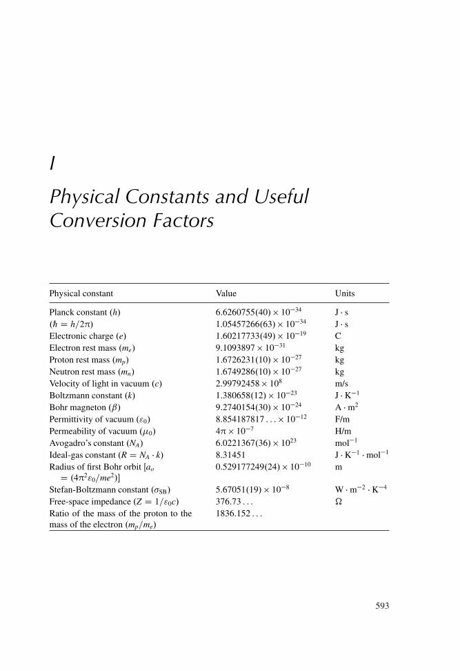
I
Physical Constants and UsefulConversion Factors
Physical constant Value Units
Planck constant .h/ 6.6260755.40/� 10�34 J � s.„ D h=2π/ 1.05457266.63/� 10�34 J � sElectronic charge .e/ 1.60217733.49/� 10�19 CElectron rest mass .me/ 9.1093897 � 10�31 kgProton rest mass .mp/ 1.6726231.10/� 10�27 kgNeutron rest mass .mn/ 1.6749286.10/� 10�27 kgVelocity of light in vacuum .c/ 2.99792458 � 108 m/sBoltzmann constant .k/ 1.380658.12/� 10�23 J � K�1
Bohr magneton .ˇ/ 9.2740154.30/� 10�24 A � m2
Permittivity of vacuum ."0/ 8.854187817 : : :� 10�12 F/mPermeability of vacuum .�0/ 4π � 10�7 H/mAvogadro’s constant .NA/ 6.0221367.36/� 1023 mol�1
Ideal-gas constant .R D NA � k/ 8.31451 J � K�1 � mol�1
Radius of first Bohr orbit Œao
D .4π2"0=me2/�
0.529177249.24/� 10�10 m
Stefan-Boltzmann constant .�SB/ 5.67051.19/� 10�8 W � m�2 � K�4
Free-space impedance .Z D 1="0c/ 376.73 : : : �
Ratio of the mass of the proton to themass of the electron .mp=me/
1836.152 : : :
593
594 Appendixes
Physical constant Value Units
Energy corresponding to 1 eV 1.602 : : :� 10�19 JEnergy of a photon with wavelenght� D 1 μm
1.986 : : :� 10�19 J
Wavenumbers corresponding to anenergy spacing of kT.T D 300 K/. Q� D kT=hc/
208.512 : : : cm�1
Atmospheric pressure .1 atmD 760 torr D 1.013 : : : bar/
1.013 : : :� 105 Pa
Answers to Selected Problems
Chapter 1
1.1. Far infrared: 1 mm – 50�m. Medium infrared: 50 � 2.5�m. Near infrared: 2.5�m � 750 nm.Visible: 750 � 380 nm. Ultraviolet: 380 � 180 nm. Vacuum ultraviolet: 180 � 40 nm. Soft x-ray:40 � 1 nm. X-ray: 1 � 0.01 nm.
1.4. For g1 D g2 one gets from Eq. (1.2.2) E2 � E1 D kT D 208.5 cm�1 so that � D .1=208.5/ cmŠ 48�m, falling in the medium infrared.
1.5. �1 D 1, �2 D � ln R2 Š 0.693, �i Š 0.01, � D �i C .�1 C �2/=2 Š 0.357, Nc D �=� lŠ 1.7 � 1017 cm�3.
1.6. Dm Š .2�=D/L Š 533 m, where Dm is the beam diameter on the moon, D is the telescope aper-ture, and L is the distance between earth and moon. The first earth-moon ranging experiment wasachieved under these conditions, using a Q-switched ruby-laser. Owing to the large beam diameteron the moon and to the surface variations over this diameter, the precision of this ranging exper-iment was rather limited .�1 m/. Using special mirrors, as beam reflectors, placed on the moonsurface by visiting astronauts, the earth-moon distance can now be measured with an accuracy ofroughly a few mm.
Chapter 2
2.1. N.�/ D 8πV �=�4 Š 1.9 � 1012 modes !
2.2. �� D �� jd�=d�j D cn=�
2��� where the relation �� D cn (cn being the light velocity in the
medium filling the black-body cavity) has been used. From Eq. (2.2.22) with the substitution� D cn=� one then obtains
�� D 8 cnh
�5
1
exp.hcn = �kT/ � 1
2.3. By imposing the condition .d��=d�/ D 0 and using the expression for �� given in the answer ofProblem 2.2, one gets the equation 5 � Œexp.hcn=�kT/� 1�� .hcn=�kT/ exp.hcn=�kT/ D 0. If one
595
596 Answers to Selected Problems
writes y D .hcn=�kT/ in the previous expression one sees that the value of y corresponding to thepeak of �� must satisfy the equation 5 � Œ1 � exp.yM/� D yM . The solution of this equation can beobtained, by a fast converging iterative procedure, as yM Š 4.965. For cn D c, c being the lightvelocity in vacuum, the wavelength, �M, at which the maximum value of �� occurs, must thensatisfy the relation (Wien’s law): �MT D hcn=yMk Š 2.3 � 10�3 m � K.
2.6. The density of the Nd3C ions, N, expressed in ions=cm3, and hence the Nd3C concentration inthe 4I9=2 manifold is given by N D 1 � 10�2 3.�=M.W./NA where � is the density, expressed
in g=cm3, M.W. is the molecular weight of YAG, and NA is Avogadro’s number. The factor 3in the previous expression accounts for the presence of three yttrium atoms per molecule. Sincethe YAG molecular weight is 594 g/mol we obtain N Š 1.38 � 1020 ions=cm�3. According toEq. (1.2.2), the fraction, f , of this population belonging to the lowest sub-level of the 4I9=2 stateis then given by
f D 1
1 C4P
iD1exp �.Ei = kT/
where Ei.i D 1–4/ is the energy separation between the higher sublevels and the ground sublevel.Given the values of Ei for these sublevels one gets f D 46%.
2.7. From Eqs. (2.4.25) and (2.3.15) one gets �in D �2
n=8 �Œg.� � �0/=�sp� where �n D c=n � �0
is the wavelength, in the medium, of an e.m. wave of frequency �0. For � D �0 and for a pureinhomogeneous broadening, using Eq. (2.4.28), we obtain the following expression for the peakcross-section �p D 0.939
�2
n=8 �
1=���0 �sp
�. For �n D 1.15�m .n Š 1/, ��
0 D 9 � 108 Hz,and �sp Š 10�7 s we then get �p Š 5.5 � 10�12 cm2.
2.8. Consider a plane wave, of uniform intensity I, crossing a surface, of area S, in a medium ofrefractive index n. The e.m. energy flux through the surface S in a time t is E D ISt and thisenergy is found, uniformly distributed, in a volume V D S.c=n/ Š t. The energy density in themedium is then �n.E=V/ D .n=c/I.
2.11. The answer is readily obtained following Example 2.13. One gets .˝=4π/ D .D=4l/2 Š 4.4�10�4 and from Eq. (2.9.4a), by a fast iterative procedure, one finds G D 1.24 � 104. The thresh-old inversion is then Nth D ln G=�pl D 4.49 � 1018 cm�3 and the maximum stored energy EM
D Nth.πD2l=4/ � h� D 1.96 J.
2.13. Under thermal equilibrium the two processes Eqs. (2.6.9) and (2.6.10) must balance each other.Thus the relation �B�ANB� NA D �BA� NBNA� must hold. At exact resonance and again at ther-mal equilibrium one has .NA�=NA/ D .NB�=NB/ D exp �.E=kT/ where E is the energy levelseparation between either one of the two-level system. We then get �B�A D �BA� .
2.14. For a Lorentzian line one has
Is D Isof1 C Œ2.� � �0/=�0�2g
We then get
˛.� � �0/ D ˛0.0/
1 C Œ2.� � �0/ =�0�2
� 1
1 C .I = Is/D
D ˛0.0/
1 C Œ2.� � �0/ =�0�2 � 1
1 C IIso
11CŒ2.���0/ = ��0�2
D
Answers to Selected Problems 597
D ˛0.0/
1 C Œ2.� � �0/ =�0�2 C .I = Iso/
2.15. On setting � D �o in the expression obtained in Problem 2.14, we get
˛p.0/ D ˛0.0/
1 C .I = Is0/
According to this equation, the saturation intensity, Is0, is the intensity of a resonant .� Š �o/
e.m. wave at which the peak saturated absorption coefficient, ˛p.0/, is half of the correspondingunsaturated value, ˛0.0/. The (1/2) power points of ˛ D ˛.� � �o/, in the expression obtained inthe previous problem, occur at frequency �0 so that Œ2.�0 ��0/=�0�
2 D 1C.I=Is0/. The saturatedlinewidth (FWHM) is then readily obtained as �sat D �0Œ1 C .I=Is0/�
1=2.
Chapter 3
3.1. The center of mass is midway between the two atoms. Considering the x-axis to be along thevibration direction with the origin at the center of mass, the restoring force on each atom is givenby F D �2k0.x � x0/, where x0 is the equilibrium coordinate of each atom. The equation ofmotion can then be written as ŒMd2.x � x0/dt2� D �2k0.x � x0/ so that the resonance frequencyis ! D Œ2k0=M�1=2.
3.2. Using the result of the previous problem we obtain k0 D .2π Q� c/2 � .M=2/ D 2, 314 J � m�2 wherethe atomic weight of the N atom has been taken to be Š 14. The potential energy of the system isthen given by U D k0.R�R0/
2=2, where R is the internuclear separation and R0 is the equilibriumvalue. For R � R0 D 0.03 nm one obtains U Š 6.5 eV.
3.6. B D „2=2I. In this expression one has I D 2MoR20, where Mo is the oxygen mass and R0 is
the equilibrium distance between oxygen and carbon. For B D 0.37 cm�1 and Mo D 16 g=mol(atomic weight) we obtain R0 D „=2 � ŒMo � B�1=2 D 0.0515 nm.
3.8. From Fig. 3.15b, for N D 1.6 � 10�18 cm�3, one gets EFc D 2.35 kT and EFv D �1.45 kT . Theoverall gain bandwidth is then Q� D .EFc C EFv/=hc D 0.9.kT=hc/ D 187.65 cm�1. [we recallthat .kT=hc/ D 208.5 cm�1 at T D 300 K].
3.9. E2 C E1 D 0.45 kT . From Eq. (3.2.2) we get .E2=E1/ D mv=mc D 6.865 where mv is the holemass and mc is the electron mass in the conduction band. From the previous two equations we getE2 D 0.392 kT and E1 D 0.0572 kT .
3.10. From Fig. 3.16 and for E � Eg D 0.45 kT Š 12 meV we obtain ˛ D ˛0 D 1.8 � 103 cm�1. Sincethe probabilities of occupation of the upper and lower laser level are given by [see Eq. (3.2.10)]
fc.E2/ D 1
1 C exp�.E2 � EFC / = kT
fv.E1/ D 1
1 C exp�.EFV � E1/ = kT
from the results of Problems 3.8 and 3.9, we obtain fc.E2/ D 0.877 and fv.E1/ D 0.8186. FromEq. (3.2.37) we then get g D ˛0Œfc.E2/� fv.E1/� Š 104 cm�1.
598 Answers to Selected Problems
3.11. � D .dg=dN/ D Œg=.N � Ntr/� D 2.6 � 10�16 cm2, where g D 104 cm�1, N D 1.6 � 1018 cm�3
and, see Example 3.7, Ntr D 1.2 � 1018 cm�3.
3.13. From Fig. 3.26, for N D 2 � 1018 cm�3, one gets EFc � E1c Š 2.8 kT Š 72 meV and EFv�E1v Š �1.1 kT Š �28.6 meV. Using the results of Example 3.9 for E1c and E1v one then obtainsEFc D 128.2 meV and EFv D �20.6 meV. According to Eq. (3.3.26) the gain bandwidth occursfor E-Eg ranging between E1 D E1c C E1v D 64.2 meV and EFc C EFv D 107.6 meV.
Chapter 4
4.3. One has T D 1 � R � A D 5 � 10�3. From Eq. (4.5.6a) the peak transmission is obtained as.TFP/p D ŒT=.1 � R/�2 D 25%. Note the strong reduction in peak transmission even for such asmall mirror loss. A comparison between Eqs. (4.5.6a) and (4.5.6) [with R1 D R2 D R] showsthat the expression for the finesse still remains that given by Eq. (4.5.14); thus F D πR1=2=.1�R/Š 312.4.
4.4. From Eqs. (4.5.8) and (4.5.3), assuming normal incidence . D 0/ and unit refractive index.nr D 1/, one gets L D c=2�fsr D 5 cm. From Eq. (4.5.13) the finesse is then obtained asF D �fsr=�c D 50. From Eq. (4.5.14), with R1 D R2 D R, we readily obtain the value ofthe mirror reflectivity as R Š 94%. From Eq. (4.5.6a), for a peak transmission of 50%, we thenobtain T D 4.24 � 10�2 and hence A D 1 � R � T D 1.76 � 10�2.
4.7. The wavefront radius of curvature, at the lens position, is given by [see Eq. (4.7.17b)] R DdŒ1 C .zR=d/2�, where zR D πw2
0=� is the Rayleigh length. To compensate this curvature, thefocal length of the lens must just equal R.
4.9. From Eq. (4.7.19) one gets w0 D �=πd Š 201�m. Assuming that the output beam forms awaist, the peak intensity will occur at this waist position and will be given by Ip D P=
πw2
0=2� Š
7.85 W=cm2. From Eqs. (2.4.10) and (2.4.6), the intensity of an e.m. wave is seen to be related tothe field amplitude E0 by I D nE2
0=2Z where Z D 1="oc Š 377 ohms is the impedance of free
space. For n D 1 we then get E0 D Œ2IZ�1=2 Š 77 V=cm.
4.11. From Eq. (4.7.27) one readily gets w02 D �f =D. The numerical aperture of a lens is definedas (see Sect. 1.4.4) N.A. D sin./, where is the half-angle of the cone formed by theaperture D seen from the central point in the focal plane. Since tan ./ D D=2f , one getsw02 D �=2 tan.sin�1 N.A./. For a small numerical aperture one has w02 Š �=2N.A.
4.13. According to Eq. (4.7.4), the beam parameter q, after the plate, is related to the input beamparameter q0 by
1
qD C C .D = q0/
A C .B = q0/
In our case q0 D �jzR, where zR D πw20=� is the Rayleigh length. Using the ABCD matrix
elements of a plate of length L and refractive index n [see Table 4.1] we obtain
1
qD �jzR
1 � j.L = nzR/
From the real and imaginary parts of the above equation, with the help of Eq. (4.7.8), one obtains
w2 D w20Œ1 C .L0=zR/
2�
R D L0Œ1 C .zR=L0/2�
Answers to Selected Problems 599
where L0 D L=n. This proves the statement of Problem 4.13. After the plate, the spot size atdistance z from the waist would then be equal to that which would occur, without the plate, at adistance z0 D .z�L/C.L=n/ D z� Œ.n�1/=n�L. At large distances from the waist, i.e. for z � zR,one then has w.z/ D .�=πw0/ � fz � Œ.n � 1/=n�Lg. The beam divergence is then d D w.z/=z and,if L zR, one has z � L and the beam divergence remains equal to .�=πw0/ i.e. it is unaffectedby the presence of the plate.
4.14. Equation (4.7.26) can be written as
zm D 11f C f
zR1
For a given value of zR1 , the denominator of the right hand side of the above equation has aminimum for f D zR1 . At this value of focal length, zm then reaches its maximum value given byzm D zR1=2.
Chapter 5
5.2. wo D pL�= 2π D 0.29 nm; ws D p
2 wo Š 0.4 mm; �c D c=2L D 150 MHz. Number ofmodes N D ��
o =.c=4L/ D 47, where .c=4L/ is the frequency spacing between two consecutivenon-degenerate modes of a confocal resonator (see Fig. 5.10a).
5.4. The curvature of the wavefront must coincide with that of the mirror, at the mirror’s location.From Eq. (4.7.13b), setting z D L=2 where L is the cavity length, one then gets
w20
�D L
2
�2R
L� 1
�1=2
The above expression gives zR D πw20=� Š 1.32 m and w0 Š 0.466 mm. The spot-size at the
mirror is then obtained from Eq. (4.7.13a) as w D w0Œ1 C .L=2zR/2/�1=2 D 0.498 mm.
5.6. Since the equiphase surfaces, at the two mirror positions, must coincide with the mirror surfaces,from Eq. (4.7.17b) one writes
�R1 D z1 C
z2R
z1
!
R2 D z2 C
z2R
z2
!
L D z2 � z1
where z1 and z2 are the coordinates of the mirrors as measured from the waist. Note the minussign in front of the term R1 in the first equation. It arises from the fact that, if e.g. mirror 1 is aconcave mirror, R1 is positive while the sign of the wavefront is negative because the center ofcurvature is to the right of the wavefront. From the above three equations one can then eliminatez2 to obtain
�R1z1 D z21 C z2
R
R2.L C z1/ D .L C z1/C z2R
600 Answers to Selected Problems
From these two equations one can eliminate z2R, to obtain z1Œ2L � R1 � R2� D L.R2 � L/. Note
that, for R1 D R2 D R, this equation gives z1 D �L=2, which shows that, in this case, the waist islocated at the cavity center. From Eq. (5.4.10) one now finds R1 D L=.1�g1/ and R2 D L=.1�g2/.The substitution of these two expressions for R1 and R2 into the previous equation then readilygives �z1.g1 C g2 � 2g1g2/ D g2.1 � g1/L.
5.7. We have g1 D 0.333, g2 D 0.75. From the expression for z1 obtained in the previous problemwe then find z1 D �0.857 m. From Eqs. (5.5.8) and (5.5.9) we also find w1 D 0.533 mm, w2 D0.355 mm and w0 D 0.349 mm.
5.9. For symmetry reasons the waist must be located at a distance Lp=2 from the lens. FromEq. (4.7.17b) one then finds that the absolute value of the wavefront’s radius of curvature, onboth sides of the lens, is given by R D .Lp=2/Œ1 C .2zR=Lp/
2�. The lens must then transform onewavefront into the other. One must then have f D R=2. Since zR D πw2
0=�, one obtains from the
previous expressions w20 D .�=2π/ŒL.4f � Lp/�
1=2. Note that the previous expression gives a realvalue of w2
0 only when Lp 4f , which represents the stability condition for our case.
5.11. One has g1 D 1 and g1 D 1 � L=.L C/ Š =L. From Eq. (5.5.8b) one then has w2 D wm D.L�=π/1=2f1=.=L/Œ1 � .=L/�g1=4. For wm D 0.5 mm, L D 30 cm and � D 633 nm, the aboveexpression gives D 1.85 cm. We then have R2 D L C D 31.85 cm, and g2 D 0.058, and,from Eq. (5.5.8a), the spot size at the plane mirror is obtained as w1 Š 0.122 mm.
5.13. In this case, from Eqs. (5.5.5) and (5.4.6) the stability condition is seen to be given by �2 <
2.2A1D1 �1/ < 2 i.e. by 0 < A1D1 < 1. Since B1D1 �A1C1 D 1, one then finds �1 < B1C1 < 0.
5.17. (1) g1 D 1, g2 D 1.25; (2) from Eq. (5.6.1): r1 D 2.24 and r2 D 1.24; (3) a1 > M21a2 D 1.8 a2;(4) M D M12M21 D 2.62, so that � D .M2�1
/=M2 D 0.85.
5.18. Positive branch confocal unstable resonator. From Fig. 5.22, for � D 0.2 and Neq D 7.5, one findsM D 1.35. It then follows that 2a2 D 2Œ2L�Neq=.M � 1/�1=2 D 4.26. To achieve a single-endedresonator one must have a1 > 2Ma2 D 5.75 cm. The radii of the two mirrors, on the other hand,must be such that L D .R1 C R2/=2 and M D �R1=R2 (note that R2 < 0). We obtain R1 D 7.7 mand R2 D �5.7 m.
5.20. (1) From Eq. (5.6.20) one gets exp �2.a=w/6 D 2�10�2 i.e. w D 2.94 mm. (2) From Eq. (5.6.21)wm D w=.M6 � 1/1=6 D 2.32 mm. (3) � D 1 � .R0=M2/ Š 0.744. (4) Since g2 D 1, fromEqs. (5.6.3) and (5.6.1) one gets M D g1f1 C Œ1 C .1=g1/�
1=2g2 from which one obtains g1 D1.0285. The radius of curvature of the convex mirror is then R1 D L=.1 � g1/ Š �17.5 m.
Chapter 6
6.1. For radial propagation, the power absorbed in the laser rod can be written as Pa D s SŒ1�exp �.2˛R/�Ie�d�, where S is the rod’s lateral surface area. Since the power entering the rod isPe D s SIe�d�, we obtain �a D Pa=Pe D s Œ1 � exp �.2˛R/�Ie�d�= s Ie�d�.
6.4. From Eq. (6.2.6) with h�mp Š 2.11 � 10�19 J Œ�mp D 940 nm� one readily gets Rcp Š 2.01�1020 cm�3s�1.
6.6. The pump efficiency is, in this case, equal to �p D �t�a�pq D 5.3%. The laser of Problem 6.4,with a pump efficiency of �0
p D 4.5%, has a threshold of P0th D 2.36 kW. With the present pump
configuration, the threshold pump power will then be Pth D��p=�
0p
�P0
th D 2.36 kW. To pump
Answers to Selected Problems 601
the laser 2 times above threshold we then need a pump power of Pp Š 4.72 kW. The area of thecollecting optics is then given by A D Pp=I Š 4.72 m2, where I is the solar intensity. If we letD and l be the rod diameter and rod length respectively, the focal lengths of the two lenses mustbe such that f1˛ D D and f2˛ D l, where ˛ is the angle which the sun’s disc subtends at theearth. One gets f1 D 0.64 m and f2 D 8.05 m. A cheaper focusing scheme could be made using aspherical mirror, with focal length f2 D 8.05 m and diameter D D .4A=π/1=2 D 2.45 m, followedby a cylindrical lens.
6.7. Rcp D �pEth=Vh�mpt, where t is the pump duration. Since h�mp D 2.11 � 10�19 J one obtainsRcp D 5.75 � 1021 cm�3s�1. The rate equation involving pumping and spontaneous decay is.dN2=dt/ D Rp � .N2=�/ whose solution, for Rp D const and t 0, is N2.t/ D Rp� Œ1�exp �.t=�/�. Assuming � D 230�s, t D t D 100�s, and with the help of the previouslycalculated value of Rcp, one gets the critical inversion as N2c D Rcp�Œ1 � exp �.t=�/� D4.66 � 1017 cm�3. If the pulse duration is increased to t0 D 300�s, the pump rate, R0
cp, toachieve the same inversion must be such that R0
cpŒ1 � exp �.t0=�/� D RcpŒ1 � exp �.t=�/�.One gets R0
cp Š 0.48 Rcp Š 2.78 � 1021 cm�3s�1. The new threshold pump energy is thenE0
p D R0
cpt0=Rcpt�
Ep Š 1.44 Ep Š 4.9 J.
6.10. From Table 6.2 one gets Nt D 9 � 1020 cm�3 so that �aNtl C � D 0.169. Assuming a �80%efficiency for the transfer optics, the pump efficiency can be taken to be �p D �t�a D �tŒ1�exp.˛l/� D 0.424 where ˛ D 5 cm�1 is the absorption coefficient at the pump wavelength (seeTable 6.2). From Eq. (6.3.25), with wp D w0, one then readily gets Pth Š 177 mW.
6.12. For a Maxwell–Boltzmann distribution one has kTe D .2=3/m�2
th=2�. Since
m�2
th=2� D
10 eV, we then get kTe D 6.67 eV.
6.15. Using Gauss’s theorem, the radially oriented electric field, at the radial coordinate r within themedium, can be expressed as E.r/ D Nier=2"0. By integration, the potential drop between walland center is readily obtained as V D NieR2=4"0 Š 4.56 � 106 V, where R is the tube radius. Thevery high value of the voltage obtained shows that there is a negligible probability for electrons todisappear at a different rate from that of the ions.
6.18. The thermal velocity is given by �th D .2E=m/1=2 D 1.87 � 108 cm=s, where m is the mass ofthe electron. For an ideal gas, the molar volume is given by V D RT=p, where R D 8.314 J �mol�1 � K�1 is the gas constant. For p D 1.3 torr Š 1.73 � 102 Pa and T D 400 K one gets V D19.2 � 106 cm3. The atomic density in the gas is then given by N D NA=V D 3.14 � 1016 cm�3
where NA is Avogadro’s constant (see Appendix I). We then obtain the electron mean free path asl D 1=N� D 638�m. From Eqs. (6.4.14) and (6.4.15), the drift velocity can then be obtained as�drift D eE l=m�th Š 1.8 � 107 cm=s .�drift=�th Š 9.6 � 10�2/.
Chapter 7
7.3. Le D L C .n � 1/l D 56.15 cm, � D 0.12, �c D 15.6 ns.
7.4. The overall lifetime of the upper laser level is such that .1=�/ D .1=�21/C .1=� 0/, where .1=�21/
is the rate of the 2 ! 1 transition and .1=� 0/ is the rate of all other spontaneous transitionsoriginating from level 2. Since the branching ratio, ˇ, is given by ˇ D .1=�21/=.1=�/ D �=�21, weget �21 D �=ˇ D 451�s. Below threshold, at steady state, one has .N1=�1/ D .N2=�21/, where �1is the lifetime of the lower laser level. Thus, for .N1=N2/ < 1%, one must have �1 < 10�2 �21 Š4.5�s. For an output power of Pout D 200 W, the rate of emission of photons from the activemedium is .d�=dt/ D Pout.2�=�2/=h� D 1.58 � 1021 photons/s. The population ending up in
602 Answers to Selected Problems
the lower laser level, per unit time, will then be dN 0=dt D .d�=dt/=Abl D 9.16 � 1020 cm�3s�1,where Ab is the effective beam area in the rod and l is the rod length. The steady-state populationN1 is then given by N1 D �1.dN0=dt/ while the upper-state population, N2, is now equal to thethreshold population, i.e., N2 D Nc Š 5.7 � 1016 cm�3. For .N1=N2/ < 1% one must now have�1 < 10�2 � Nc=.dN0=dt/ Š 0.6�s. (The actual lifetime �1 for Nd:YAG is � 100 ps).
7.7. The minimum threshold power is given by Pmth D Pth � �i=� D 2.75 kW where �i is the internalloss .�i D 0.02/ and � is the total loss .� D 0.32/. At a pump power of Pp D 140 kW we thenhave xm D Pp=Pmth D 50.9. From Eq. (7.5.5) one finds Sop D 6.135, so that �2op D 2Sop�i D0.25. The corresponding optimum output power is obtained from Eq. (7.5.6) as Pop D 16.78 kW.We have T2op D 1 � exp.��2op/ Š 0.25. Since the peak intensity in the focal plane of a lens
is proportional to .M2�1/=M2 (see Sect. 5.6.3) the ratio between the two intensities is .Iop=I/ D
PopT2op=PT2 D 16.78 � 0.22=12 � 4.45 D 0.777.
7.8. The lens of focal length f can be divided into two, closely spaced, lenses each of focal length2f . The radius of curvature of the wavefront at the lens position is given by R D .L=2/�f1 C ŒzR=.L=2/�2g, with zR D w2
0=�, where w0 is the spot size at each of the two mirrors.For symmetry reasons, the wavefront between the two lenses must be plane. Thus, one musthave R D 2f D 50 cm. Using this value of R in the previous expression one finds zR D 25 cmi.e. w0 D 290�m. The spot size at the lens position is then w D p
2w0 D 410�m.
7.10. The minimum threshold pump power for zero output coupling is P0mth D Pth�i=� D 12.5 mW
[note that P0mth should not be confused with Pmth given by Eq. (7.3.32)]. At Pp D 1.14 W one
has xm D 91.2. From Eq. (7.5.5) one then gets Sop D 8.54 i.e. � 02op D 2Sop�i D 8.5%. To
calculate the output power we note that the total loss is now given by � 0 D�� 0
2op=2�
C �i D4.75% and the amount by which threshold is exceeded is x0 D x�=� 0, where x and � are thecorresponding values obtained in Example 7.4 (x D 30 and � D 3%). We get x0 D 19 so that,
from Eq. (7.3.34), we find y0 D 15.6. The expected power is then P0out D Pout.y0=y/
�� 0
2op=�2
�D
510 mW where Pout, y, and �2 are the corresponding values obtained in Example 7.4 .Pout, D500 mW, y D 26, �2 D 5%/. We should note that, indeed, our optimization procedure hasresulted in a value of P0
out (slightly) larger than Pout.
7.12. The lens of focal length f can be divided into two, closely spaced, lenses each of focal length f 0 D2f . The spot size between the two lenses is wa and, for symmetry reasons, the wavefront is plane.The position of the two plane mirrors must also correspond to a beam waist. From Eq. (4.7.26)we then find that the distance between each plane mirror and the corresponding lens f 0 is givenby zm D f 0=Œ1 C .f 0=zR/
2� where, in our case, zR D w2a=� Š 581 cm. For f 0 D 2f D 42 cm
one finds zm Š 41.8 cm. The spot size on each mirror is then obtained from Eq. (4.7.28) asw0 D .�=πwa/f 0 Š 100�m.
7.15. One has �2 D � ln.1 � T2/ Š 5.1%. To avoid oscillation on the TEM01 mode, the requireddiffraction loss per pass for this mode must be � 7.45%. From Fig. 5.13b and for g D 1 �.L=R/ D 0.8 one then finds N D a2=�L 2, i.e. a p
2�L Š 1 mm.
7.17. Nc D �=�el Š 4 � 109 ions=cm3; Rcp D Nc=� Š 8 � 1017 cm�3s�1; � D c=2L Š 1.5�108 Hz; .Rp=Rcp/ D exp
h2�= ��
0
�2ln 2
iD 1.005.
7.19. One has L D n.�=2/, where n is an integer number. According to this equation, if L is increasedby �=2, the oscillation wavelength will increase by � D �=n. Since �� D c we then get� Š �.�=�/� D ��=n. From the relation � D n.c=2L/ we then obtain � Š �.c=2L/.
Answers to Selected Problems 603
7.21. Assume that a transmission peak of the FP etalon is made coincident with the central mode. Thetwo adjacent longitudinal modes, which are frequency spaced by � D c=2L, will not oscillateif the FP transmission at these two frequencies, T.�/, is such that T.�/ exp.�pNl � �/ 1.We obtain T.�/ 0.8. From Eqs. (4.5.6) and (4.5.14), with R1 D R2 D R, one gets T.�/ D1=Œ1 C .2F=π/2 sin2 �� where � D 2πL0�=c with L0 Š nrLet D 2.9 cm (Let is the thicknessand nr is the refraction index of the etalon). We get � D πL0=L D 9.1 � 10�1 rad and sinceT.�/ 0.8, we obtain .2F=π/2 sin2 � Š .2F=π/2�2 0.25, i.e. F .0.5π=2�/ D 8.63.Equation (4.5.14), for R1 D R2 D R, can then be written as .1 � R/ D πR1=2=F from which, byan iterative procedure, one gets R Š 0.7. We must also ensure that the mode near the next peak of
the FP etalon is below threshold. This occurs if expŒ� 2�fsr=��0
�2 ln 2� � exp.�pNl � �/ 1
i.e. for2�fsr=�
�0
�2 ln 2 0.223, where �fsr Š .c=2nrLet/ is the FP free-spectral-range.
We obtain Let Œln 2=0.223�1=2 c=nr��0 Š 10.4 cm which shows that the above condition is
satisfied in our case.
Chapter 8
8.2. Since k�L0 D . =2/, one finds V D �=4n30r63.
8.4. From Fig. 8.14, for f � D f � D 2.3 and x D 10 kW=2.2 kW D 4.55, we obtain Ni=Np Š 1.89, sothat, from Fig. 8.11, we find �E Š 0.76. Since �2 D 0.162 and Ab D 0.23 cm2 (see Example 7.2),from Eq. (8.4.20) one finds E Š 18 mJ which gives an average output power of < P >D Ef D180 W, i.e., very close to the c.w. value (202 W, see Fig. 7.5). Since � D 0.12 (see Example 7.2)and Le D L.n � 1/l Š 56 cm (where n D 1.8 is the refractive index of the YAG crystal), we get�c D Le=c� D 15.6 ns and, from Eq. (8.4.21), �p Š 90 ns.
8.7. (1) Since tp is much shorter than the upper state lifetime, one has .dN=dt/ D Rp i.e. N D Rpt.Since Rptp D 4Nth, where Nth is the threshold inversion, the time at which threshold is reachedis tth D tp=4. (2) The time behavior of the net gain is then given by gnet D �.N � Nth/l D.4�Nthl/.t � tth/=tp where tth D tp=4. (3) Neglecting saturation, one has .d�=dt/ D gnet�=tT ,where tT is the transit time. Using the expression for net gain just derived, we find, by integration,�.t0/ D �i expŒ.4�Nthl/ � .t02=2tptT /� where t0 D t � tth and �i Š 1. (4) At the end of thepump pulse one has t0 D 3tp=4 and, from the above expression for �.t0/ one gets .9�Nthl=8/ �.tp=tT / D ln.�p=20/ where �p is given by Eq. (8.4.14). Using this last expression one findstp D tT.8=9�/ ln.�p=20/, where � D .� ln T2/=2 D 0.35. To calculate �p from Eq. (8.4.14)one notes that Ni=Np D 4 and VaNp D �A=� where A is the beam area. Thus one finds that�p D 5.54 � 1010 and, since tT D 22.7 ps, it follows tp D 1.25 ns.
8.12. Equation (8.6.14) can be expressed more conveniently as E.t/ / exp .�� t2/ exp.j!0t/ where� D ˛ � jˇ, i.e. it can be transformed into a Gaussian pulse with a complex Gaussian parameter� . Its Fourier transform can then be written as E.! �!0/ / exp �.! �!0/
2=4� D exp �fŒ.!�!0/
2=4.˛2 C ˇ2/� � .˛ C jˇ/g. The power spectrum will then be jE.! � !0/j2 / exp �Œ.!�!0/
2˛=2.˛2 Cˇ2/�. If we now write jE.!�!0/j2 / exp � �4.! � !0/2 ln 2=!2
L
, where!L is
the bandwidth, a comparison of the two above expressions gives !2L D .8 ln 2/˛Œ1 C .ˇ2=˛2/�.
This equation, with the help of expression Eq. (8.16.15) for ˛ and using the relation �L D!L=2π, then leads to Eq. (8.6.16).
8.14. The average intensity is < I >D1R0
IpIdI=1R0
pIdI D I0, and the required probability is given by
p D1R
2I0
pIdI=1R0
pIdI D exp.�2/ D 0.135.
604 Answers to Selected Problems
8.16. In our case we have 2�t D 2� � kP while, in the fast saturable absorber case, one can write[see Eq. (8.6.20)] 2�t D 2� � 2� 0 .P=Ps/. A comparison of these two expressions shows thatk is equivalent to 2� 0=Ps. According to Eq. (8.6.22) the pulse duration can then be written as
�p Š .0.79=�0/2g0
0=kPp�1=2 where Pp is the peak power. For a hyperbolic secant function,
the peak power is related to the pulse energy by E D 1.13 Pp�p. From the above two expressionswe get �p Š .0.79=�0/
22g0
0=k�.1.13=E/ Š 3.5 fs.
8.17. From Eq. (8.6.35) with �00 D ˇ00l one gets l D .ı�p=�p/1=2 �
��2
p =ˇ00�/2
p2 ln 2 Š 0.46 mm,
where ˇ00 is the GVD.
Chapter 9
9.5. The emission solid angle is ˝ D πD2=4l2 Š 2.83 � 10�3 sr. Assuming a Gaussian line, fromEq. (2.9.4b), with � Š 1, one gets G Š 1.37 � 104, i.e. Nth D ln G=�pl Š 2.38 � 1019 cm�3,where �p Š 4 � 10�20 cm2 for Nd:glass (see Table 9.3). We then obtain E D NthVh� D 12.7 Jwhere V D 2.83 cm3. For Nd:YAG, at the same value of the solid angle and assuming a Lorentzianline, we get from Eq. (2.9.4a), with � D 1, G Š 2.5 � 104 i.e. Nth D 3.61 � 1018 cm�3 so thatE Š 1.91 J.
9.7. Neglecting ground state and excited state absorption and under mode-matching conditions.w0 Š wp/ the threshold pump power, from Eq. (6.3.20), is seen to be given by Pth D.�=�p/.h�p=�/
πw2
0=�e�. We have � D .�2=2/C �i D 1.5 � 10�2, �p Š 1 � exp �.˛pl/ Š 0.86
where ˛p D 5 cm�1 is the pump absorption coefficient, h�p Š 3.1 � 10�19 J, � D 67�s, w0 D60�m and �e D 4.8 � 10�20 cm2. We thus obtain Pth D 190 mW.
9.8. Pth D Œ.� C �a/=�p�.h�p=�/Œπ�
w20 C w2
p
�=2.�e � �ESA/�.
9.9. Pth D .�=�p/.h�p=�/Œπ�
w20 C w2
p
�=2.�e � kST�T�T/�.
9.12. �s D dP=VdI D .h�=eV/Œ� ln R=.˛L � ln R/�. For � D 850 nm, h�=e D 1.46 eV, and V D 1.8 Vone gets �s Š 64%.
9.13. One must have w20jjh1 C
�z�=πw2
0jj�
2i�
D w20?h1 C
z�=πw20?�2i�
, which gives z Dπw0jjw0?=�. For the given values of w0jj, w0? and �, one obtains z D 4.6�m (note the veryshort distance).
9.15. .2πn1L=�/ D 2 i.e. n1 D �=πL Š 8.22 � 10�4.
Chapter 10
10.4. If we let �.� � �0/ be the unsaturated cross section of ArC, oscillation will occur up to the n-thmode, away from the central mode, such that �.n�/�Nl � , where� is the frequency spacingbetween consecutive longitudinal modes, N is the unsaturated inversion, l is the length of theactive medium, and � is the cavity loss. The unsaturated cross section is then given by �.n�/ D�p exp �Œ2n�=��
0
�2 ln 2�. In this expression �p is the peak cross section and, with the laserpumped three-times above threshold, one has �pNl D 3� . From the above three expressions
one finds 3 exp �Œ2n�=��0
�2 ln 2� 1, from which one gets n Œln 3= ln 2�1=2��
0 =2��.
Answers to Selected Problems 605
Since ��0 D 3.5 GHz and � D c=2L D 150 MHz (L is the cavity length), one finds n 14.7.
The number of oscillating modes is then Nosc D 2n C 1 D 29.
10.6. For a homonuclear molecule consisting of two atoms of mass M, the vibrational frequency,according to Eq. (3.1.3), is given by �0 D .1=2π/Œ2k0=M�1=2 where k0 is the elastic constant.For M Š 14 a.u. Š 2.32 � 10�26 kg and Q�0 D 2300 cm�1 one finds k0 D 2180 Nm�1.
10.8. For the symmetric stretching mode, the carbon position is fixed and the force acting on eachoxigen atom is F D �k.x�x0/, where k is the elastic constant and x0 is the equilibrium separationbetween carbon and oxygen. It then follows that the resonance frequency of this mode is givenby !1 D Œk=MO� where MO is the mass of the oxygen atom. For Q�1 D 1337 cm�1 and MO D16 a.u. Š 2.65 � 10�26 kg one finds k D 1683 Nm�1.
10.10. Let x0 be the equilibrium distance between one of the oxygen atoms and the carbon atom. Atransverse displacement of the carbon atom by y would correspond to an elongation d of the
spring given by d D x2
0 Cy2�1=2 � x0. For y � x0 one then gets d Š y2=2x0 from
which one sees that the force produced by the spring would be proportional to y2. This impliesthat the harmonic oscillator model, for oscillation along the y-direction, cannot be derived viathe simplified spring-model considered in this problem.
10.13. All ro-vibrational lines will merge together when the collision-broadened linewidth, �c,becomes comparable with the frequency separation between rotational lines. Assuming �c D�r D 60 GHz, from the given value of �c one gets a total pressure of p Š 13 997 torr D18.4 atm. From Fig. 10.11 one then sees that the width of the gain curve, �0, corresponds toJ0 values ranging between J0 Š 11 and J0 Š 41, i.e., J0 Š 30. From the solution of Problem10.11 one finds that the rotational constant, B, of a CO2 molecule is B Š 0.3 cm�1. The width�0 of the gain curve is then given by �0 D 2BJ0 Š 60B Š 18 cm�1.
10.16. The energy which is left, after reaction, as vibrational energy is E� D3P0
� N.�/�E where
N.�/ is the population of the vibrational level, with vibrational quantum number �, and E isthe energy spacing between vibrational levels (assumed the same for all levels). On the other
hand, the total energy of reaction, Et, is, on the other hand, given by Et D H3P0
� N.�/ where
H Š 3E is the reaction energy. From the above equations one finds that � D .E�=Et/
D3P0
� N.�/� =3P0
� N.�/ D 68.5%.
Chapter 11
11.3. The field of the beam, along the C direction, due to the superposition of the two beams of theinterferometer, can be written as Ec D KAE.t/C KBE.t C �/. If the power reflectivity of mirrorS1 is 50% and neglecting, for simplicity, any phase shift arising from reflection at mirrors S1, S2,and S3, we can assume KA D KB D K. We then get < Ic.t/ >D< Ec.t/E�
c .t/ >D 2 jKj2 f < I >CReŒ� .1/.�/�g where < I >D< E.t/E�.t/ >D< E.t C �/E�.t C �/ > and Re stands for real
part. With the help of (11.3.4) and (11.3.9) one then gets < Ic.t/ >D 2 jKj2 < I > f1 Cˇ� .1/
ˇcos
Œ< ! > � � �.�/�g. Around a given time delay � , since bothˇ� .1/
ˇand � are slowly-varying
functions of � , one then has Imax D< Ic.t/ >maxD 2 jKj2 < I > Œ1 Cˇˇ� .1/ .�/
ˇˇ�, Imin D<
Ic.t/ >minD 2 jKj2 < I > Œ1 �ˇˇ� .1/ .�/
ˇˇ�, and Vp D
ˇˇ� .1/ .�/
ˇˇ.
606 Answers to Selected Problems
11.5. For a Gaussian spectral output, � .1/ .�/ will also be a Gaussian function, i.e. it can be written as� .1/ D exp �Œ.�=�co/
2 ln 2�, where �co, the coherence time, is defined as in Fig. 11.1. Accordingto (11.3.28) one then has �� D 1=4π�� . In our case we have �� D �L while the variance �� ofthe function Œ� .1/�2 D exp �Œ2.�=�co/
2 ln 2� is �� D �co=2p
ln 2. From the above expressions weobtain �co D p
ln 2=2π�� Š 13.25�s and Lco D c � �co Š 3.98 km.
11.7. I0 D 2Pi=π.�f=πw0/2. To avoid excessive diffraction losses and creation of diffraction rings from
beam truncation by the finite lens aperture, DL, one should choose a large enough DL, typicallyDL D πw0 [see Eq. (5.5.31)]. From the above expressions we then find I0 D .2=π/PiD2
L=.�f /2
while, from (11.4.4), with D D DL, we find I0 D .π=4/PiD2L=.�f /2.
11.9. If we let x and y be the coordinates along the smaller and larger dimensions respectively of thenear-field pattern, one has Wx0 D 0.5 cm and Wy0 D 2 cm. From (11.4.19) one then has Wx.z D3 m/ Š 3.28 cm, while from the equivalent equation along the y-direction, one gets Wy.z D3 m/ Š 2.16 cm.
Chapter 12
12.1. Since w0 D 0.54 mm, one has w.z D 1 m/ D w0 Œ1 C .z=zR/�1=2 D 0.83 mm and R.z D 1 m/ D
zŒ1 C .z=zR/2�1=2 Š 1.74 m, where zR D w2
0=� Š 86.1 cm. The lens of focal length f canbe divided into a first lens, of focal length f1 D R D 1.74 m, to compensate for the wavefrontcurvature, and a second lens, of focal length f2 D f1 �f=.f1�f / Š 10.61 cm, to focus the beam. Toa good approximation, the waist position then occurs at a distance of zm Š f2 Š 10.61 cm fromthe original lens. The spot-size of the embedded Gaussian beam is w0
0 Š .�= w/�f2 Š 0.043 mm
and the corresponding spot-size parameter is W00 D
pM2w0
0 Š 0.274 mm.
12.3. One has �s D h�=� Š 4.71 J=cm2 and S D D2=4 Š 63.6 cm2, so that �out D Eout=S Š7.07 J=cm2. The total energy available in the amplifier is Eav D h�NV D S�s ln G0 D 415 J,where N is the initial inversion and V is the volume of the amplifier. To calculate the requiredinput energy, (12.3.12) can be solved for �in to give �in D ŒfŒexp.�out=�s/ � 1�=G0g C 1�Š 2.95 J=cm2 which results in Ein D �in S D 187.8 J. Thus, out of an available energy of 415 J,the energy extracted from the amplifier is Eex D Eout � Ein Š 262.2 J. Note that the length ofthe amplifier does not enter into this calculation.
12.9. With the help of (12.4.27a), substitution of (12.4.29) into (12.4.2) gives PNL D
."0d=2/
(3P1
i Ei.z/ expŒj.!it � kiz/�C c.c.
) 2
. After manipulation of the right hand side of the
above equation, it can easily be seen that, since !1 D !3 � !2, the only term at frequency!1 is PNL
!1D ."0d=2/
˚E�
2 .z/E3.z/ expŒj.!3 � !2/t � j.k3 � k2/z�C c.c.�. Using the relation
!1 D !3 � !2, and with the help of (12.4.27b) one then readily obtains (12.4.30).
12.11. From (12.4.58a) the second harmonic conversion efficiency is obtained as � D I2!=I!.0/ DˇE0
2!
ˇ2=ˇE0
! .0/ˇ2 D Œtanh.z=lSH/�
2. From (12.4.52), taking into account the fact that that E!.0/
is related to the incident intensity I D I!.0/ by E!.0/ D .2ZI/1=2, where Z D 1="0c Š377 ohms is the free-space impedance, one gets lSH Š �no=Œ2πdeff .2ZI/1=2� D 2.75 cm whereno is the ordinary refractive index of KDP at frequency !. Substituing this value of lSH into theabove expression for �, assuming z D 2.5 cm, one gets � D 51.9%.
Index
Absorption efficiency, 214Airy, 490, 497Alexandrite, 212, 214, 216Ambipolar diffusion, 246Amplified spontaneous emission (ASE)
Gaussian approximation, 559intensity, 557, 558Lorentzian and Gaussian lines, 558, 559spectral emission, z-direction, 557, 558
Anti-resonance-Fabry–Perot-saturable absorber(A-FPSA), 353
Ar-ion laser-pumped cw dye laser, 404Arc discharge, 233Argon laser
air- and water-cooled argon lasers, 442collision process, 439, 440energy levels, 439, 440high-power water-cooled ArC laser
tube, 441–442ophthalmology, 442spectroscopic properties, 434, 441upper state excitation, 440
Atoms and ions radiationabsorption and stimulated emission
absorption measurement, 41allowed and forbidden transitions, 36–37Dirac delta function, 33Einstein thermodynamic treatment, 41–43Gaussian line, 39–40homogeneous broadening, 37inhomogeneous broadening, 38Lorentzian line, 35monochromatic electromagnetic (e.m.) wave,
32–33
oscillating dipole moment, 34photon flux, 37–38radiation interaction, 41time-varying interaction energy, 33total line shape function, 39
blackbody radiation theoryenergy density, 18Planck hypothesis and field quantization,
24–25Rayleigh–Jeans and Planck radiation formula,
22–23rectangular cavity modes, 19–22spectral intensity, 18
degenerate levelsabsorption coefficient, 60Boltzmann equation, 58two level system, 58
gain saturation, homogeneous lineamplifier saturation fluence, 69four-level system, 67–68unsaturated gain coefficient, 68
homogeneous broadeningcollision broadening, 43
normalized spectral lineshape, 45inhomogeneous broadening, 47–49, 69–70nonradiative decay and energy transfer
collisional deactivation, 50combined effects, 56–57cooperative up-conversion process, 55dipole-dipole interaction, 54–55multiphonon deactivation, 53superelastic collision, 50
607
laser linewidth vs. temperature, 47natural broadening, 46
608 Index
thermal activation, 51optically dense medium decay
apparent threshold, 73directionality property, 72gas and solid state lasers, 76Lorentzian line, 72–73mirrorless lasers, 75radiation trapping, 71saturation intensity, 74
saturation of absorption, homogeneous lineabsorption cross section, 65gain coefficient/absorption measurement, 66population difference, 67saturation intensity, 65two-level system interaction, 64unsaturated absorption coefficient, 66
spontaneous emissionallowed and forbidden transitions, 31–32atom energy, 28quantum electrodynamics approach, 30–31radiated power, 27–28radiative emission lifetime, 28time behavior, 29
strongly coupled levelsabsorption coefficient, 62Alexandrite laser, 63Boltzmann statistics, 60–61Nd:YAG laser, 63
Autocorrelation function, 554
Bernard–Duraffourg condition, 107, 123Bessel function, 303Born approximation, 239Bragg, 325, 420Bragg regime, 324, 325, 369Brewster’s angle, 209, 210, 286, 287, 360Bulk semiconductors
absorption and gain coefficientsBernard–Duraffourg condition, 106–107GaAs semiconductor, 109–110III–V semiconductors, 105inverted semiconductor, 106joint density of states, 104vs. injected carrier density, 109
electronic statesBloch wave functions, 93conduction band, 93–94III–V compounds, 96split-off band, 97valence band, 93–94wave functions, 94–95
spontaneous emission and nonradiative decaydeep trap recombination, 111–112qualitative behaviour, 110–111
thermal equilibrium
hole density, 100level occupation probability, 98, 100, 118n-type-doping, 98p-type doping, 99Pauli exclusion principle, 98quasi-Fermi levels, 99–100, 119
Byer, R.L., 230, 297
Cascading process, 455Casperson, L.W., 261, 276, 557Cerullo, G., 200Chemical lasers
applications, 464atomic fluorine and hydrogen, 462cascading phenomenon, 463–464definition, 461population inversion, 463, 464supersonic-diffusion HF laser, 464transitions, 463vibrational levels, pumping, 462, 463
Chemical pumping, 207Chester, A.N., 193Chirped-pulse-amplification
Erbium-doped fiber amplifiers (EDFA), 515–516femtosecond laser pulse, 514master-oscillator power-amplifier (MOPA), 512NOVA system, 512, 513peak-power, 515pulse compression, 513pulse expansion, 513–514
Clay, R.A., 267Close-coupled configuration, 208–209CO laser
anharmonic pumping, 455longitudinal flow, 456partial inversion, 455vibrational-rotational transitions, 454
CO2 laserBoltzmann distribution, 447capillary waveguide lasers, 450–451decay process, 446, 447decay time, 446diffusion-cooled area-scaling laser, 452direct electron collisions, 446efficiency, 448fast axial flow, 451–452linewidth, Doppler effect, 448modes of vibration, 445probability, 447resonant energy transfer, N2 molecule, 446rotational level population, 447, 448sealed-off lasers, 450slow axial flow, 449–450transverse-flow, 452–453

Index 609
transversely excited atmospheric pressure (TEA)laser, 453, 454
vibrational-energy levels, 445Coherent waves, divergence properties, 492Colliding-pulse mode-locked (CPM) rhodamine 6G
dye laser, 366Collision broadening, lineshape calculation
autocorrelation function, 554correlation and lineshape function, 555phase jumps plot, 554, 555power spectrum, 553, 554signal wave, 553Wiener–Kintchine theorem, 554, 555
Continuous laser pumping, 404Continuous wave laser behavior
Fabry–Perot etalons, 292–293four-level laser
change of intensity, 258–259critical/threshold inversion, 265differential equations, 260diode pumping, 274Gaussian-beam pumping, 274–276laser slope efficiency, 266logarithmic loss per pass, 258longitudinal efficiency, 276–277mode distribution, 270mode energy density, 256mode-matching condition, 276output power, 261population inversion, 259–260pump rate, 264–265, 271–272radial and longitudinal coordinates, 271resonator optical length, 259Rigrod analysis, 260saturation power, 272self-terminating, 264slope efficiency, 273, 275spontaneous emission, 257steady-state population, 264stimulated emission, 257–258threshold pump power, 272unidirectional ring resonator, 276
frequency-pulling and monochromaticitycavity mode frequency, 297laser frequency, 297–298linewidth, 298–299quantum and technical noise, 299spectral width, 298
intensity noise and intensity noise reductionantiphase dynamic, 306autocorrelation function, 304mode-partition-noise, 306relative intensity noise (RIN), 304–306
laser frequency fluctuation and stabilizationelectric field, 302–303
Fabry–Perot (FP) interferometer, 301–302frequency noise spectrum, 301long-term drifts, 300offset frequency, 301Pound–Drever technique, 302, 303short-term fluctuations, 300spectral power density, 301
laser tuningbirefringent filter, 286diffraction grating, 285free spectral range, 287Littrow configuration, 285
mode-selecting scheme, 291multimode oscillation
gain profile vs. pump rate, 287–288laser gain coefficient, 288spatial hole burning, 289–290spectral hole burning, 290standing-wave pattern, 289
optimum output couplinglamp-pumped Nd:YAG laser, 285normalized output power vs. normalized
transmission, 284output power, 284–285relative insensitivity, 285
quasi-three-level laserGaussian transverse profile, 280ground state absorption, 282minimum threshold power, 281normalized output power, 281population inversion, 263pump rate, 280–281slope and transverse efficiency, 282space-independent model, 279–280stimulated emission and absorption, 262thermal equilibrium, 261
single-transverse-mode selection, 290–291unidirectional ring resonators
dye laser, 296Faraday rotator, 294–295longitudinal dc magnetic field, 294Nd:YAG laser, 296–297polarization rotation, 295transverse gain distribution, 297
Copper vapor laserscopper atoms, energy levels, 437Copper-HyBrID laser, 438, 439industrial applications, 439schematic construction, 438
Damped sinusoidal oscillation, 316–317deBroglie wavelength, 93, 238
Dexter, D.L., 54Diffraction theory, 10–11Diffusion-cooled area-scaling laser, 452
610 Index
Dirac, 24, 33, 34, 39, 42Directionality
half-angle beam divergence, 489M2 factor and spot-size parameter
beam divergence, 492beam quality, 494beam variance, 492, 493broad area semiconductor laser, 494–495Gaussian beam, 493, 494multimode laser beam, 494spatial frequency variance, 493
partial spatial coherence, 491–492perfect spatial coherence
Airy formula, 490beam divergence, 490, 491diffraction-limited beam, 491Gaussian beam, 490, 491light intensity distribution, 490
Doppler broadening, 206Drever, R.W.T., 302, 303Duraffourg, G., 106Dye lasers
characteristicsapplications, 404flashlamp pumping, 403gain coefficient, 402nonradiative decay, 401transverse pump configuration, 403
chemical structure, 397, 398photophysical properties, organic dyes
decay process, 400, 401energy levels, 399, 400Franck–Condon principle, 400free-electron model, 398, 399intersystem crossing process, 401optical and spectroscopic parameters,
401, 402rhodamine 6G, 397, 398
e-beam pumping, 206Einstein, A., 2, 3, 24, 41–43Electrical pumping
arc discharge, 233ballast resistance, 233, 234electron energy distribution
CO2 laser, 243–244crude approximation, 243electron temperature, 242–243energy redistribution, 242He–Ne laser, 244–245Maxwell–Boltzmann (MB) distribution function,
242, 243electron impact excitation
Born approximation, 239exchange collision, 239
polychromatic electron source, 238qualitative behavior, 237surplus energy, 240threshold energy, 237transition cross section, 238
glow discharge, 233ionization balance equation
ambipolar diffusion, 246electron–ion recombination, 245free fall model, 246Tonks–Langmuir theory, 246, 247
longitudinal and transverse discharge, 233–234near-resonant energy transfer, 235, 236pump rate and pump efficiency, 248–249radio-frequency transverse excitation, 234scaling laws, electrical discharge lasers, 247semiconductor laser pumping, 232thermal and drift velocities
definition, 240inelastic, elastic and electron–electron collisions,
240, 242kinetic energy, 240, 241
Electron–phonon dephasing collisions, 103Embedded Gaussian beam, 506–507Energy levels, radiative and nonradiative transitions
absorption and gain coefficientsBernard–Duraffourg condition, 106–107, 123GaAs semiconductor, 109–110GaAs/AlGaAs, 123III–V semiconductors, 105inverted semiconductor, 106joint density of states, 104, 121–122vs. injected carrier density, 109vs. photon energy, 108, 124
Born–Oppenheimer approximation, 83density of states, 97, 116–118electronic states
bandgap energy difference, 113Bloch wave functions, 93, 114conduction band, 93–94III–V compounds, 96quantum-well state, 115split-off band, 97valence band, 93–94wave functions, 94–95
harmonic oscillator expression, 82metallo-organic chemical vapor deposition
(MOCVD), 113polyatomic molecule, 84potential energy curves, 82quantum wires (QWR) and quantum dots (QD),
126–128radiative and nonradiative decay, 91–92rotational energy levels, 85, 86Schrodinger’s equation, 83
Index 611
spontaneous emission and nonradiative decaydeep trap recombination, 111–112modal gain, 112qualitative behaviour, 110–111
stimulated transitions, 101–103, 119–121Franck–Condon principle, 87–88Gaussian function, 88infrared active, 89P branch lines, 89–90pure rotational transitions, 87, 91R branch lines, 89–90rotational-vibrational transitions, 87, 89selection rules, 89, 91vibronic transitions, 87–88
strained quantum wells, 125–126thermal equilibrium
hole density, 100level occupation probability, 86, 98, 100, 118n-type-doping, 98p-type doping, 99Pauli exclusion principle, 98population distribution, 87probability level occupation, 118quasi-Fermi levels, 99–100, 119
vibrational energy levels, 82, 84Excimer laser
applications, 460charge-transfer state, 459definition, 458energy states, 457, 458excitation mechanisms, 459–460KrF laser, 459properties, 458rare-gas-halide excimer, 458–459TEA configuration, 453, 460
Fabry–Perot (FP) interferometer, 301–302properties
electric field amplitude, 143finesse, 145intensity transmission vs. incident wave
frequency, 144mirror absorption, 146multiple-beam interference, 142–143power transmission, 143–144spherical mirrors, 142transmission maximum, 144transmission minima, 145
spectrometer, 146–147Fabry–Perot resonator, 164Fan, T.Y., 230Faraday rotator, 294–296Fast axial flow CO2 laser, 451Fermi levels, 407Fermi–Dirac statistics, 98, 118
Findlay, D., 267First-order perturbation theory, 549Flash-lamp pumped configuration, 387Forster, 54Forster-type dipole–dipole interaction, 387Forster-type ion–ion interaction, 388Four-level laser
rate equationschange of intensity, 258–259differential equations, 260logarithmic loss per pass, 258output power, 261population inversion, 259–260quantum electrodynamics, 257
resonator optical length, 259Rigrod analysis, 260spontaneous emission, 257stimulated emission, 257–258
space-dependent modeldiode pumping, 274Gaussian-beam pumping, 274–276longitudinal efficiency, 276–277mode-matching condition, 276pump rate, 271–272saturation power, 272slope efficiency, 273, 275threshold pump power, 272unidirectional ring resonator, 276
space-independent modelcritical/threshold inversion, 265laser slope efficiency, 266pump rate, 264–265self-terminating, 264steady-state population, 264
Fourier series, 339, 342Fourier transform, 170, 304–305, 343, 344Fox, A.G., 184, 193Franck–Condon factor, 91, 563Franken, P.A., 516Free-electron laser (FEL)
basic structure, 465Compton scattering, 468oscillation frequency, 465, 466properties, 469Raman scattering, 468spectral width, 466spontaneously emitted radiation, 466–467stimulated emission process, 465,
467, 468wavelength, 465, 466
Free-space propagation, 506Fresnel number, 194, 195, 198, 290–291Fresnel–Kirchoff integral, 148, 150, 154Fundamental mode-locking, 345
612 Index
Gain-guided laser, 416, 417Gas lasers
ion laserair- and water-cooled argon lasers, 442collision process, 439, 440He–Cd laser, 442–444high-power water-cooled ArC laser tube,
441–442ophthalmology, 442spectroscopic properties, 434, 441upper state excitation, 440
molecular gas lasersBoltzmann distribution, 447capillary waveguide lasers, 450–451CO laser, 454–456decay process, 446, 447decay time, 446diffusion-cooled area-scaling laser, 452direct electron collisions, 446efficiency, 448excimer laser, 457–460fast axial flow, 451–452linewidth, Doppler effect, 448material-working applications, 456modes of vibration, 445N2 laser, 456–457optical pumping, 444probability, 447resonant energy transfer, N2 molecule, 446rotational level population, 447, 448sealed-off lasers, 450slow axial flow, 449–450transverse-flow, 452–453transversely excited atmospheric pressure (TEA)
laser, 453, 454vibrational-energy levels, 445
neutral atom lasercopper vapor laser, 437–439current density vs. population, 435, 436de-excitation process, 435electron configuration, 433energy levels, He–Ne laser, 433–434excited (21S) state population, 435hard-sealed laser design, 434, 435transitions, spectroscopic properties, 434
Gas-dynamic pumping, 207Gaussian approximation, 559Gaussian beams
ABCD law, 156–157free space propagation
beam divergence, 155field amplitude, 153Rayleigh range, 154transverse and longitudinal phase factor,
154–155
higher-order modes, 158–159lowest-order mode
beam spot size, 152complex parameter, 151eigensolution, 150–151wave’s radius of curvature, 151, 152
Gaussian lines, 558, 559Giordmaine, J.A., 516Glow discharge, 233Graded-index separated-confinement heterostructure
(GRINSCH), 414, 415Group delay dispersion (GDD)
dispersion compensation, 360–361laser pulse propagation, 584pulse compression, 539, 540pulse duration, 358–360pulse expansion, 542
Group velocity dispersion (GVD), 358, 538, 584
Hamiltonian interaction, 101, 103Harmonic mode-locking, 345Haus, H.A., 348, 351, 575He–Cd laser
applications, blue/UV beam, 444energy levels, 442, 443Penning ionization process, 442–443tube type construction, 443
Helium–Neon (He–Ne) lasercavity length, 436characteristic features, 435current density vs. population, 435, 436de-excitation process, 435electron configuration, 433energy levels, 433–434excited (21S) state population, 435hard-sealed laser design, 434, 435oscillation, 432, 437transitions, spectroscopic properties, 434
Helmholtz equation, 20Henry, C.H., 299Hermite polynomials, 158, 182, 184Hermite–Gaussian solutions, 175, 176, 190Higher-order coherence
correlation function, 590degree of coherence, 589–590normalized n-th order coherence function, 590–591
Homogeneous lineactive mode-locking
field amplitude, 576maximum intensity, pulse, 579round trip loss, 578single-pass electric-field transmission, 576spectral amplitude, 576, 577time delay, 577
passive mode-locking, 580–581
Index 613
Huygens’ wavelet, 148Huygens–Fresnel propagation equation, 167Huygens–Fresnel–Kirchoff integral, 149Index-guided lasers, 416, 417Interference fringes, 480Inverse Fourier transform, 305
Kane, T.J., 297Koechner, W., 268, 270, 333Kubodera, K., 229Kuizenga, D.J., 348, 575
Lamp-pumped solid state lasers, 214Laser amplifier, 5Laser beam transformation
amplificationamplifier medium, 507chirped-pulse-amplification, 512–516gain coefficient, amplifier length, 511losses, 509–511maximum energy, 512output laser energy fluence vs. input fluence, 510parasitic oscillations, 511, 512rate of change, population inversion, 507saturation energy fluence, 508stimulated emission and absorption, 508
dielectric polarization, 516dispersion relation, 535Maxwell’s equations, 526nonlinear polarization, 516, 517, 527parametric oscillation
basic equations, nonlinear parametric interaction,529
doubly resonant, 525–526, 531nonlinear crystal, 524, 525optical parametric oscillator, 525, 529polarization component, 524, 525singly resonant, 526synchronous pumping, 526threshold pump intensity ratio, 532
pulse compressionexperimental setup, 536grating-pair, 540group delay dispersion (GDD), 539, 540group velocity dispersion (GVD), 538instantaneous carrier frequency, 537optical-fiber compression scheme, 541self-phase modulation, 536
pulse expansiondiffraction gratings, 541–543grating-pair compressor, 540, 541group delay dispersion (GDD), 542
second-harmonic generation (SHG)anisotropic crystal, 519
characteristic length, 533coherence length, 518conversion efficiency, 523double refraction phenomenon, 523index ellipsoid, 519, 520intensity vs. crystal length, 534, 535nonlinear crystals, 523, 524nonlinear optical coefficients, 521, 522normal (index) surface, 519, 520phase-matching angle, 521, 522polarization wave oscillation, 2! frequency, 517propagation constant, 518second harmonic polarization component, 520,
521Laser beams properties
brightness, 498–499coherence time, 484directionality
M2 factor and the spot-size parameter, 492–495partial spatial coherence, 491–492perfect spatial coherence, 489–491
intensity, 475laser light vs. thermal light
degree of spatial coherence, 501He–Ne laser, 502, 503output power, 502spatial and frequency filter, 501, 502
laser speckleapparent grain size, scattering surface, 498free-space propagation, 495, 496grain-size calculation, 496–498image-forming, 495, 496noise, 498pattern and physical origin, 495
monochromaticity, 475–476nonstationary beams, 485oscillation bandwidth, 484spatial and temporal coherence
degree of spatial coherence, 479degree of temporal coherence, 478measurement, 480–483mutual coherence function, 479normalized function, 477, 478single-mode and multimode lasers, 485–488stationary beam, 477thermal light source, 488–489
statistical properties, laser light and thermal lightaverage intensity, 500fluctuations, 500, 501single mode laser, 500thermal light source, 501
Laser operationbeam properties
brightness, 11–13directionality, 10–11
614 Index
monochromaticity, 9radiation characteristics, 8short time duration, 13spatial and temporal coherence, 9–10
Boltzmann statistics, 4–5critical inversion, 5–6laser elements, 14logarithmic losses, 6population inversion, 5pumping schemes
four-level laser schemes, 7population inversion, 6–7quasi-three-level lasers, 8three-level laser schemes, 7two-level saturation, 6
spontaneous and stimulated emission, absorptionabsorption cross section, 3Einstein A coefficient, 2energy difference, E2–E1, 1–2non-radiative decay, 1stimulated emission cross section, 3
types, 14Laser oscillation, 386Laser pulse propagation, dispersive/gain medium
dispersion length, 585electric field, 583, 584group delay dispersion (GDD), 584group velocity, 584instantaneous frequency, 586pulse broadening, 584pulse magnitude, 585spectral amplitude, 587
Laser pumpingabsorption coefficient, 215–216laser diode pumps
beam divergences, 217–218index-guided laser, 217monolithic and stacked bars, 218monolithic array, 217, 218spectral emission, 218–219thermoelectric cooler, 219types, 217vs. lamp-pumping, 230–232
longitudinal pumpinganamorphic prism pair, 220–222cylindrical lenses, 220–221cylindrical microlens, 222, 223double-ended pumping, 219multimode optical fiber, 223optical-to-optical efficiency, 223plane-concave resonator, 219reshaped beam, 223–224single-stripe configuration, 220
pump rate and pump efficiencyabsorption efficiency, 227
cladded rod, 228Gaussian distribution, 226spot size, 226–227
pumping parameters vs. laser wavelengths, 216quantum well (QW) lasers, 215–216threshold pump power
four-level laser, 228–229quasi-three-level laser, 230
transverse pumping, 224–225Laser quantum efficiency, 266Li.T., 184, 185, 193Line broadening mechanisms
homogeneous broadeningcollision broadening, 43
normalized spectral lineshape, 45inhomogeneous broadening, 47–49
Linear stability analysis, 317Liquid lasers, 205Littrow configuration, 285Lorentz, H.A., 35Lorentzian lines, 301, 302, 558, 559Louisell, W. H., 484
Maiman, T.H., 377Manley–Rowe relations, 529, 535Maxwell equations, 19, 547Maxwell–Boltzmann (MB) distribution function, 242,
243, 248Michelson interferometer, 482, 483Microwave amplification by stimulated emission of
radiation (Maser), 5Mid Infrared Advanced Chemical Laser (MIRACL),
207Miller, R.C., 516Miyazawa, S., 229Mode-locking, 13, 14
active mode-lockingelectric field, 346–347FM mode-locking, 349–350Gaussian distribution, 348mode-coupling mechanism, 347noise pulse, 349Pockels cell electro-optic phase modulator, 350steady-state pulse duration, 348types, 346
femtosecond mode-locked lasers, cavity dispersiondispersion compensation, 360–361phase-velocity, group-velocity and
group-delay-dispersion, 356–358pulse duration, group-delay dispersion, 358–360soliton-type mode-locking, 361–363
frequency-domain descriptionamplitude vs. frequency, 340
laser linewidth vs. temperature, 47natural broadening, 46
Index 615
cavity mode amplitudes, 342dye/tunable solid-state lasers, 342equal-amplitude mode-spectrum, 343FWHM, 341, 343, 344Gaussian distribution, 343–344spectral intensity, 344time behavior, 341total electric field, 340transform-limited pulse, 343
passive mode lockingfast saturable absorber, 351–353Kerr-lens-mode-locking (KLM), 353–354slow-saturable-absorber, 354–356types, 350–351
regimes and systemsactive ML and cw pump, 365–366CPM Rhodamine 6G dye laser, 366pulsed pump, 364Ti:sapphire KLM laser, 366–367
time-domain picturedefinition, 344–345fast cavity shutter, 345repetition rate, 345–346
Molecular transitions, radiative transition rateelectrical dipole moment, 561electronic wave functions, 563molecular wave functions, 562oscillating dipole moment, 561rotational-vibrational transitions, 562–563
Monochromaticity, 475–476Moulton, P.F., 275
N2 laser, 456–457Neodymium lasers
crystalline hosts, 384Nd:glass, 383–384Nd:YAG
applications, 382–383diode-pumping, 382energy levels, 380, 381lamp pumping, 382level notation, 380nonradiative decay, 381optical and spectroscopic parameters, 381, 382pump bands, 381slope efficiency, 382
Nonradiative decay and energy transfercombined effects, 56–57mechanisms
collisional deactivation, 50cooperative up-conversion process, 55dipole–dipole interaction, 54–55multiphonon deactivation, 53near resonant energy transfer, 52superelastic collision, 50
thermal activation, 51Nonstationary beams, 485
Optical Kerr effect, 353, 361–363Optical parametric generator (OPG), 525Optical parametric oscillator, 525, 529Optical pumping, incoherent light source
pump efficiency and rate, 213–215pump light absorption, 211–212pumping systems
close-coupled configuration, 208–209cw lasers, 210, 211double-ellipse, 209elliptical cylinder, 208pulsed lasers, 210rod-shaped laser medium, 210
Optically dense medium decayamplified spontaneous emission (ASE)
apparent threshold, 73directionality property, 72gas and solid state lasers, 76Lorentzian line, 72–73mirrorless lasers, 75saturation intensity, 74
radiation trapping, 71Oscillating bandwidth, 476Otsuka, K., 229Output coupling efficiency, 266
p-n homojunction laser, 408Paraxial-ray approximation, 132Passive optical resonators
cavity photon decay time, 164concentric and confocal resonator, 165diffraction losses, 163dynamically and mechanically stable resonators
geometrical-optics, 188, 189minimum spot size, 187misalignment sensitivities, 188–189pump power, 188thermal lens, 186, 187
eigenmodes and eigenvaluesHuygens–Fresnel propagation equation, 167–168lens-guide structure equivalent, 167propagation kernel, 168round-trip phase shift, 169total single-period phase shift, 168two-mirror resonator, 167
finite aperturebeam propagation, 185diffraction loss vs. Fresnel number, 184–185equivalent lens-guide structure, 183Fox–Li iterative procedure, 184kernel, 186
616 Index
geometrical-optics descriptioncounter-propagating spherical waves, 190magnification factor, 191round-trip logarithmic loss, 192single-ended resonator, 191
hard-edge unstable resonators, 196infinite aperture
amplitude factor, 180complex amplitude distribution, 176eigenvalue phase, 180field distribution, 175frequency spectrum, 181–182propagation kernel, 175q-parameter calculation, 176–177resonance frequency, 180–181round-trip matrix, 177spot size, symmetric resonator, 178–179standing- and traveling-waves, 182–183
mode electric field, 164photon lifetime and cavity Q
linewidth, 170, 171Lorentzian line shape, 170–171mirror and scattering losses, 169
plane-parallel resonator, 164positive and negative branch resonators, 189ring resonator, 166stability condition
ABCD matrix, 172–173g1 and g2 parameters, 174Sylvester’s theorem, 173two-mirror resonator, 171–172
variable-reflectivity unstable resonatorscentral reflectivity and cavity magnification, 198field reflectivity, 196Gaussian reflectivity profile, 197–198round-trip losses, 197round-trip magnification, 196–197, 200super-Gaussian reflectivity profile, 198–199
wave-optics descriptioncoupling losses vs. magnification factor, 195–196equivalent Fresnel number vs. eigenvalue
magnitude, 194–195Fox–Li iterative procedure, 193Huygens–Fresnel diffraction equation, 192–193intensity profile, 193–194lowest-order mode, 194, 196mode intensity distribution, 193transverse modes, 194
Patel, C.K.N., 449Perturbation method, 549Physical constants and conversion factors, 593–594Planck hypothesis and field quantization
harmonic oscillator, 24–25Heisenberg uncertainty principle, 25quantum field theory, 24
Plane-parallel resonator. See Fabry–Perot resonatorPockels cell, 322–323, 350Pound–Drever technique, 302, 303Power quantum efficiency, 214Preionization techniques, 454Pulse compression
experimental setup, 536grating-pair, 540group delay dispersion (GDD), 539, 540group velocity dispersion (GVD), 538instantaneous carrier frequency, 537optical-fiber compression scheme, 541self-phase modulation, 536time behavior, 537
Pulsed laser pumping, 403Pulsed pumping system, 213Pump transfer systems
longitudinal pumpinganamorphic prism pair, 220–222cylindrical lenses, 220–221cylindrical microlens, 222, 223double-ended pumping, 219multimode optical fiber, 223optical-to-optical efficiency, 223plane-concave resonator, 219reshaped beam, 223–224single-stripe configuration, 220
transverse pumping, 224–225
Q-switchingacousto-optic Q-switches, 324–325active Q-switching theory
continuous wave pumping, 336–337critical inversion, 329–330energy utilization factor (�E/ vs. Ni/Np , 331, 332laser output pulse peakpower, 330output energy, 331time delay, 332–333
dynamic behaviorfast-switching, 320slow-switching, 321
electro-optical Q-switching, 322–323operating regimes, 328–329rotating prisms, 323–324saturable-absorber Q-switch
saturation intensity, 325, 326single-mode operation, 327
Q-switching and mode-locking operation, 379Quantum well (QW) lasers, 215–216Quantum wires (QWR) and quantum dots (QD)
configurations, 126gain coefficient vs. emission wavelength, 127planar array, 128qualitative behavior, 126, 127
Quasi-three-level laser
Index 617
rate equationspopulation inversion, 263stimulated emission and absorption, 262thermal equilibrium, 261
space-dependent modelGaussian transverse profile, 280ground state absorption, 282minimum threshold power, 281normalized output power, 281pump rate, 280–281slope and transverse efficiency, 282
space-independent model, 279–280
Radiative efficiency, 214Ray and wave propagation
diffraction optics, paraxial approximationABCD matrix, 149, 150field distribution, 148Fresnel approximation, 149Huygens principle, 150monochromatic wave, 147wave equation, 148, 149
Fabry–Perot interferometerelectric field amplitude, 143finesse, 145intensity transmission vs. incident wave
frequency, 144multiple-beam interference, 142–143power transmission, 143–144spectrometer, 146–147spherical mirrors, 142transmission maximum, 144transmission minima, 145
Gaussian beamsABCD law, 156–157free space propagation, 153–155higher-order modes, 158–159lowest-order mode, 150–153
matrix formulation, geometrical opticsforward and backward propagation, 136free-space propagation, 135optical element, 131–132paraxial-ray approximation, 132ray matrix, 133, 134spherical mirror, 133spherical wave propagation, 136–137
multilayer dielectric coatingsabsorption loss, 140antireflection coating, 139, 142high-reflectivity laser mirrors, 139low index layer, 140, 141peak reflectivity, 141power reflectivity, 140V-coating, 142
wave reflection and transmission
Brewster’s angle, 138–139electric field reflectivity, 137–138intensity reflectivity, 138reflected and refracted beams, 138–139
Rayleigh range, 154Rayleigh–Jeans and Planck radiation formula, 22–23Rectangular cavity modes
density, 21Helmholtz equation, 20Maxwell equation, 19
Rensch, D.B., 193RF excited waveguide CO2 laser, 450, 451Rigrod analysis, 260Rigrod, W.W., 260, 266
Sapphire, 378Schawlow, A.L., 298, 299, 301Schawlow–Townes theory, 298, 301Schottky theory, 246Schrodinger equation, 238Second-harmonic generation (SHG)
anisotropic crystal, 519characteristic length, 533coherence length, 518conversion efficiency, 523double refraction phenomenon, 523field variables, 533index ellipsoid, 519, 520intensity vs. crystal length, 534, 535nonlinear crystals, 523, 524nonlinear optical coefficients, 521, 522normal (index) surface, 519, 520phase-matching angle, 521, 522photon momentum, 519propagation constant, 518second harmonic polarization component, 520, 521
Self-phase-modulation (SPM), 362–363Semiclassical treatment, radiation interaction
electric dipole interaction, 547Hamiltonian, 547, 548perturbation method, 549time-independent Schrodinger wave-equation, 548transition probability, 549, 551wave-function, 548, 549
Semiconductor lasersapplications, 425–426devices and performances
divergence properties, 418, 419Fabry–Perot type, 419Fermi energy, 418output power vs. input current, 417, 418stripe-geometry configuration, 416
distributed feedback and distributed Bragg reflectorlasers
Bragg condition, 421, 422
618 Index
�=4�shift, 420, 421refractive index change, 421, 422uniform grating, 419–421
double-heterostructure laserband structure, 409, 410GaAs laser, 412–413internal quantum efficiency, 411lattice-matching condition, 410refractive index, 409, 410schematic diagram, 409threshold current density vs. thickness,
410, 411transverse beam profile, 409, 410
homojunction laser, 407–408principle of operation
recombination-radiation process, 406valence and conduction band, 405, 406
quantum well lasersbeam confinement, 414energy bands, Alx/Ga1�xAs-GaAs, 414, 415In0.5GaP0.5/In0.5(Ga0.5�xAlx/P MQW structure,
415structure, 414, 415
vertical cavity surface emitting lasersbottom emitting design, 423, 424fabrication, 424–425schematic representation, 423
Semiconductor quantum wellsabsorption and gain coefficients
Bernard–Duraffourg condition, 123GaAs/AlGaAs, 123joint density of states, 121–122vs. photon energy, 124
electronic statesbandgap energy difference, 113Bloch wave functions, 114quantum-well state, 115
thermal equilibrium, 118–119SF6 molecule, 84Siegman, A.E., 190, 194, 195, 348, 575Single-longitudinal-mode selection
Fabry–Perot etalons, 292–293mode-selecting scheme, 291unidirectional ring resonators
dye laser, 296Faraday rotator, 294–295Nd:YAG laser, 296–297transverse gain distribution, 297
Single-mode and multimode lasersmagnitude, 487, 488Schwartz inequality, 488transverse modes, 486
Snell’s law, 132, 139Solid-state lasers, 205
alexandrite laser
energy level diagram, 392flashlamp-pumped laser, 394Franck–Condon principle, 392optical and spectroscopic parameters, 393
pumping, 393tunable laser, 391
Cr:LISAF and Cr:LICAF, 396–397electric dipole transition, 377Er:YAG and Yb:Er:glass, 386–387fiber lasers
cladding pumping scheme, 390conventional single-mode fiber, 389end-pumped single-mode fibers, 390pump beam, 389up-conversion laser scheme, 390, 391
neodymium laserscrystalline hosts, 384Nd:glass, 383–384Nd:YAG, 380–383
rare earth and transition metals, 376, 377ruby laser
application, 379–380energy levels, 378optical and spectroscopic parameters, 379pump bands, 378
titanium sapphire laserabsorption and fluorescence bands, 395configuration-coordinate model, 394, 395continuous wave (CW), 395–36octahedral configuration, 394optical and spectroscopic parameters, 393, 395
Tm:Ho:YAG, 387–388Yb:YAG laser
absorption lines, 385energy level diagram,
384, 385longitudinal pumping configuration, 385optical and spectroscopic parameters, 384, 385quasi-three-level laser scheme, 384vs. Nd:YAG, 385–386
Space dependent rate equationsfour-level laser
active medium volume, 567effective volume, 566, 567minimum pump threshold, 569, 570outside and inside energy density, 566plane wave, 565, 566population inversion, 565, 568pump rate, 568saturation power, 569steady state average population, 568, 569stimulated process, 565total number of cavity photons, 566
phonon terminatedvibronic laser, 392
splitting, 3d energy states, 394
Index 619
uniform pumping, 569quasi-three-level laser
minimum pump threshold, 573saturation power, 572stimulated emission and absorption, 571
Stable resonatorsdynamically and mechanically stable resonators
geometrical-optics, 188, 189minimum spot size, 187misalignment sensitivities, 188–189one-way matrix, 188thermal lens, 186, 187
finite aperturebeam propagation, 185diffraction loss vs. Fresnel number, 184–185equivalent lens-guide structure, 183Fox–Li iterative procedure, 184kernel, 186
infinite apertureamplitude factor, 180complex amplitude distribution, 176eigenvalue phase, 180field distribution, 175frequency spectrum, 181–182propagation kernel, 175q-parameter calculation, 176–177quadratic equation, 175–176resonance frequency, 180–181round-trip matrix, 177spot size, symmetric resonator, 178–179standing- and traveling-waves, 182–183
Sylvester’s theorem, 173
Thermal light sourcecoherence time, 488degree of spatial coherence, 488, 489temporal coherence, 488
Time-independent Schrodinger wave-equation, 548Tm:Ho:YAG laser, 387–388Tonks–Langmuir theory, 246, 247Townes, C.H., 298, 299, 301Transfer efficiency, 214Transient laser behavior
acousto-optic Q-switches, 324–325active mode-locking
electric field, 346–347FM mode-locking, 349–350mode-coupling mechanism, 347noise pulse, 349Pockels cell electro-optic phase modulator, 350steady-state pulse duration, 348types, 346
active Q-switching theorycontinuous wave pumping, 336–337
critical inversion, 329–330energy utilization factor (�E/ vs. Ni/Np, 331, 332initial inversion, 329, 336laser output pulse peak power, 330output energy, 331time delay, 332–333
cavity dumping, 368–369dynamic behavior, Q-switching process, 319–321dynamical instabilities and pulsations, 318–319electro-optical Q-switching, 322–323femtosecond mode-locked lasers, cavity dispersion
dispersion compensation, 360–361phase-velocity, group-velocity and
group-delay-dispersion, 356–358pulse duration, group-delay dispersion, 358–360soliton-type mode-locking, 361–363
frequency-domain description of mode-lockingamplitude vs. frequency, 340cavity mode amplitudes, 342dye/tunable solid-state lasers, 342equal-amplitude mode-spectrum, 343FWHM, 341, 343, 344Gaussian distribution, 343–344spectral intensity, 344time behavior, 341total electric field, 340transform-limited pulse, 343
gain switching, 337–338mode-locking regimes and systems
active ML and cw pump, 365–366CPM rhodamine 6G dye laser, 366Ti:sapphire KLM laser, 366–367
operating regimes, Q-switched lasers, 328–329passive mode locking
fast saturable absorber, 351–353Kerr-lens-mode-locking (KLM), 353–354self-focusing, 354slow-saturable-absorber, 354–356types, 350–351
relaxation oscillationsdamped relaxation oscillation, 315linearized analysis, 315–317population inversion, 314–315step-function pump rate, 313total inversion and photon number, 313, 314
rotating prisms Q-switch, 323–324saturable-absorber Q-switch, 325–327time-domain picture of mode-locking, 344–346
Transition cross section, absorption and gaincoefficient
absorption measurement, 41Gaussian line, 39–40homogeneous broadening, 37inhomogeneous broadening, 38total line shape function, 39
Third order dispersion (TOD), 359, 361
620 Index
Transition probability, 549, 551Transverse efficiency, 266Transverse-flow CO2 laser, 452–453Transversely excited atmospheric pressure (TEA) laser,
453, 454
Unstable resonatorsgeometrical-optics description
counter-propagating spherical waves, 190magnification factor, 191round-trip logarithmic loss, 192single-ended resonator, 191
hard-edge unstable resonators, 196positive and negative branch resonators, 189variable-reflectivity unstable resonators
central reflectivity and cavity magnification, 198field reflectivity, 196Gaussian reflectivity profile, 197–198peak mirror reflectivity, 200
round-trip losses, 197round-trip magnification, 196–197, 200super-Gaussian reflectivity profile, 198–199coupling losses vs. magnification factor, 195–196equivalent Fresnel number vs. eigenvalue
magnitude, 194–195Fox–Li iterative procedure, 193Huygens–Fresnel diffraction equation, 192–193intensity profile, 193–194lowest-order mode, 194, 196mode intensity distribution, 193transverse modes, 194
Wiener–Kintchine theorem, 554, 555
X-ray lasers, 469–471X-ray pumping, 206
Young’s interferometer, 480


![Principles of Lasers - ABM-PK [PAKISTAN] · PDF filePrinciples of Lasers FIFTH EDITION Orazio Svelto Polytechnic Institute of Milan and National Research Council Milan, Italy Translated](https://img.pdfslide.us/doc/110x75/5a9e3b257f8b9a21488d8794/principles-of-lasers-abm-pk-pakistan-of-lasers-fifth-edition-orazio-svelto-polytechnic.jpg)