Principles of Fluorescence Techniques 2009 … Fluorescence Principles II: David Jameson Time-Resolved Fluorescence and Quenching Principles of Fluorescence Techniques 2009 Chicago,

Basic Fluorescence Principles II: David Jameson

Time-Resolved Fluorescence and Quenching

Principles of Fluorescence Techniques 2009 Chicago, Illinois April 8-10, 2009

David Jameson

Principles of Fluorescence Techniques 2009

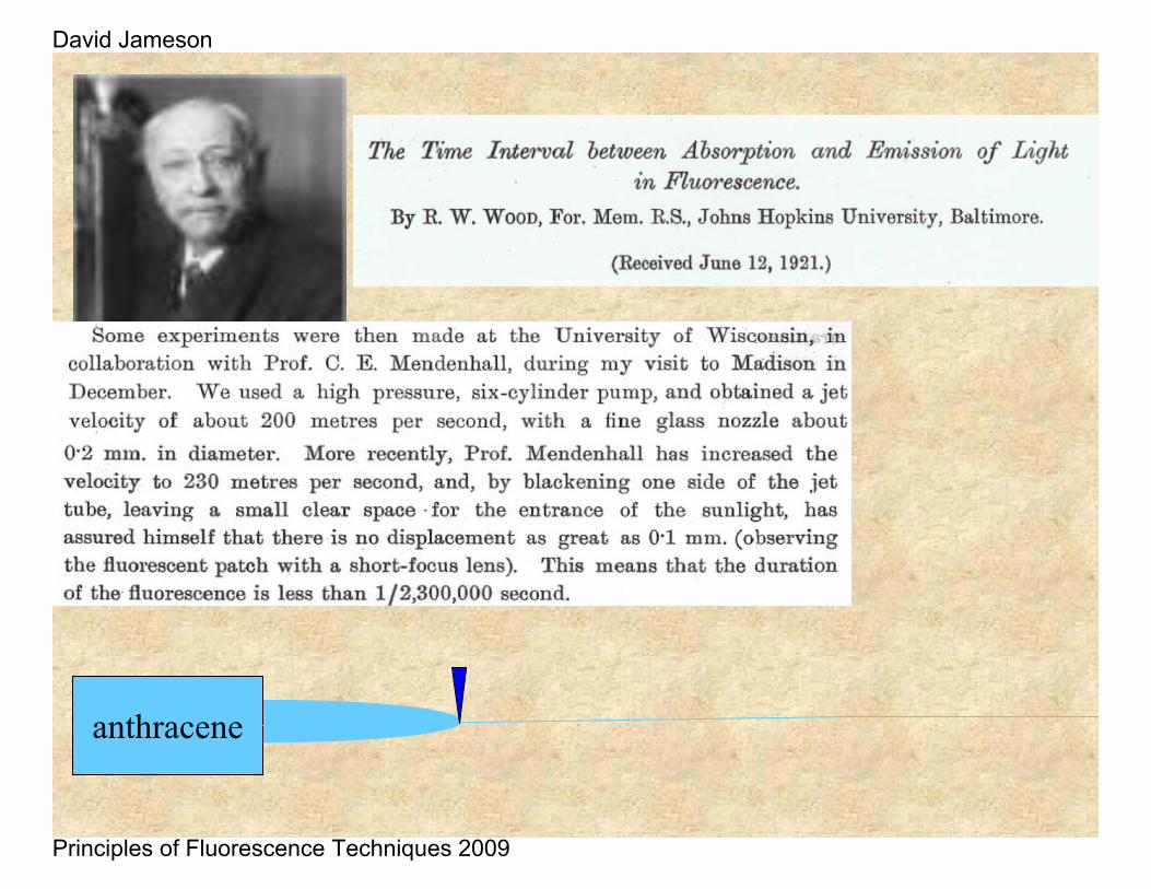
anthracene

David Jameson


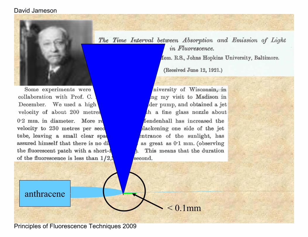
anthracene< 0.1mm

David Jameson


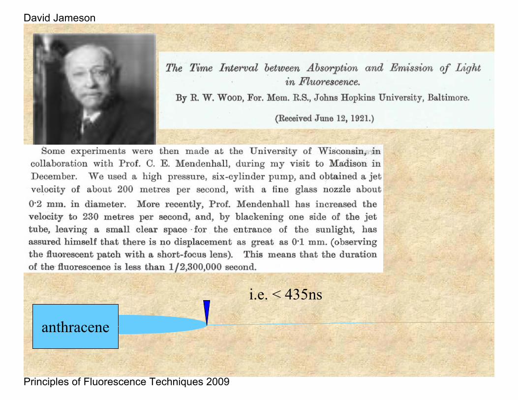
i.e. < 435ns

anthracene

David Jameson


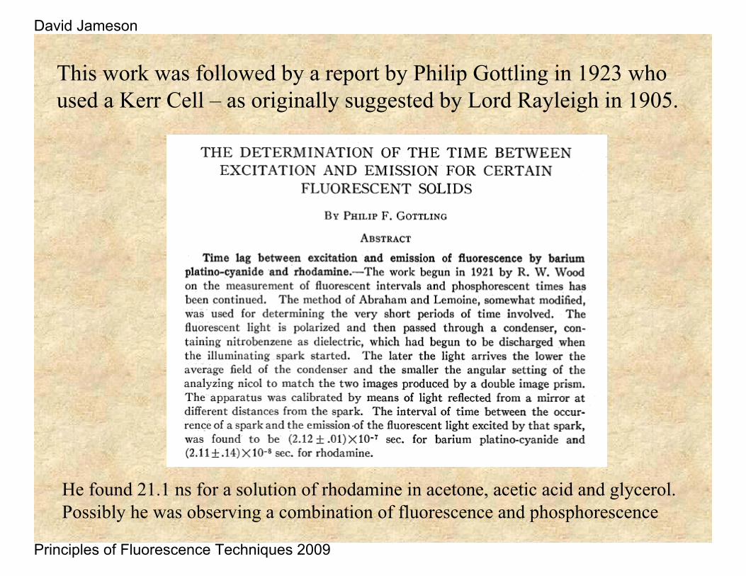
This work was followed by a report by Philip Gottling in 1923 who used a Kerr Cell – as originally suggested by Lord Rayleigh in 1905.

He found 21.1 ns for a solution of rhodamine in acetone, acetic acid and glycerol. Possibly he was observing a combination of fluorescence and phosphorescence

David Jameson


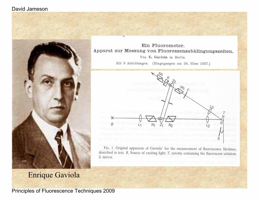
Enrique Gaviola

David Jameson


David Jameson


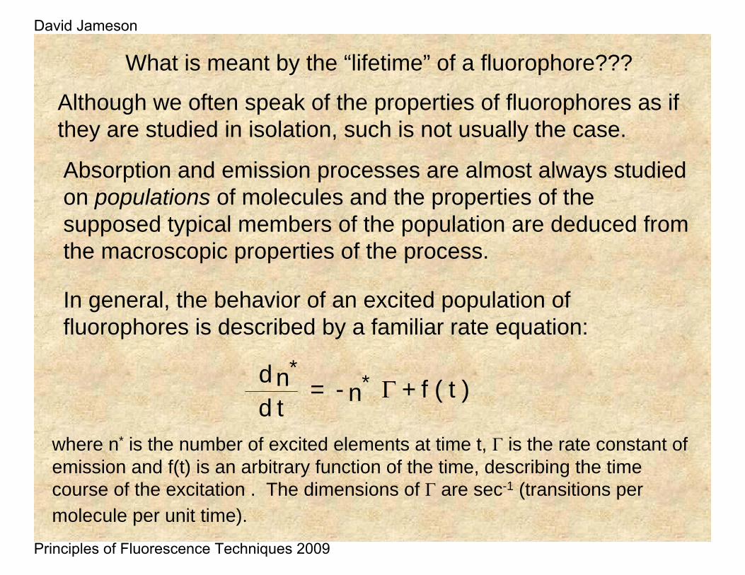
What is meant by the “lifetime” of a fluorophore???

Although we often speak of the properties of fluorophores as if they are studied in isolation, such is not usually the case.

) t ( f + n - = tdn d *

*Γ

In general, the behavior of an excited population of fluorophores is described by a familiar rate equation:

where n* is the number of excited elements at time t, Γ is the rate constant of emission and f(t) is an arbitrary function of the time, describing the time course of the excitation . The dimensions of Γ are sec-1 (transitions per molecule per unit time).

Absorption and emission processes are almost always studied on populations of molecules and the properties of the supposed typical members of the population are deduced from the macroscopic properties of the process.

David Jameson


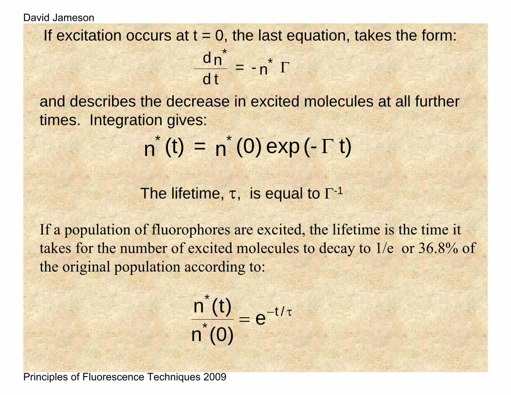
If excitation occurs at t = 0, the last equation, takes the form:

n - = tdn d *

*Γ

and describes the decrease in excited molecules at all further times. Integration gives:

t) (- exp )0( n = (t) n ** Γ

The lifetime, τ, is equal to Γ-1

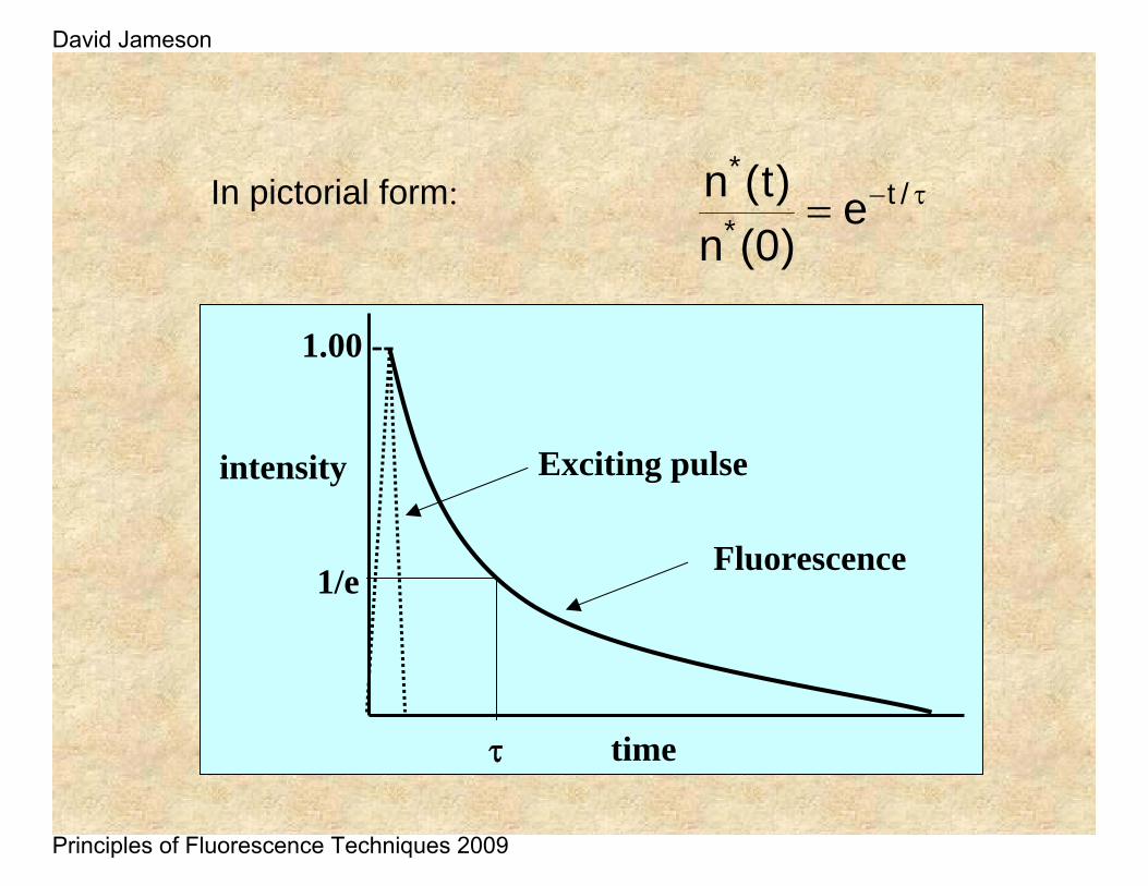
If a population of fluorophores are excited, the lifetime is the time it takes for the number of excited molecules to decay to 1/e or 36.8% of the original population according to:

τ−= /t*

*e

)0(n)t(n

David Jameson


time

intensity

1.00 --

1/e

Exciting pulse

Fluorescence

τ

τ−= /t*

*e

)0(n)t(nIn pictorial form:

David Jameson


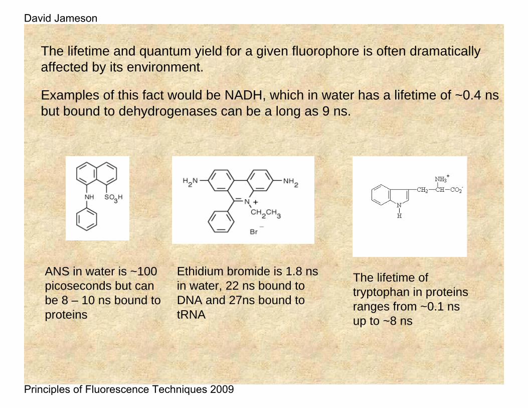
The lifetime and quantum yield for a given fluorophore is often dramatically affected by its environment.

Examples of this fact would be NADH, which in water has a lifetime of ~0.4 ns but bound to dehydrogenases can be a long as 9 ns.

ANS in water is ~100 picoseconds but can be 8 – 10 ns bound to proteins

Ethidium bromide is 1.8 ns in water, 22 ns bound to DNA and 27ns bound to tRNA

The lifetime of tryptophan in proteins ranges from ~0.1 ns up to ~8 ns

David Jameson


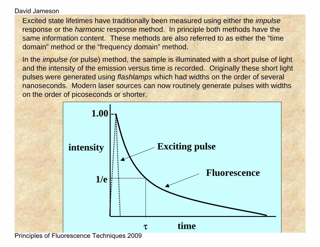
Excited state lifetimes have traditionally been measured using either the impulseresponse or the harmonic response method. In principle both methods have the same information content. These methods are also referred to as either the “time domain” method or the “frequency domain” method.

In the impulse (or pulse) method, the sample is illuminated with a short pulse of light and the intensity of the emission versus time is recorded. Originally these short light pulses were generated using flashlamps which had widths on the order of several nanoseconds. Modern laser sources can now routinely generate pulses with widths on the order of picoseconds or shorter.

time

intensity

1.00 --

1/e

Exciting pulse

Fluorescence

τ

David Jameson


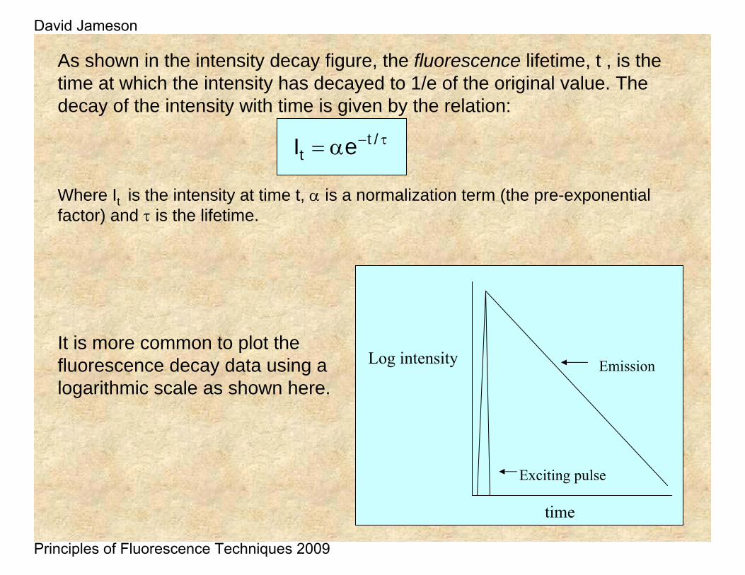
As shown in the intensity decay figure, the fluorescence lifetime, t , is the time at which the intensity has decayed to 1/e of the original value. The decay of the intensity with time is given by the relation:

Where It is the intensity at time t, α is a normalization term (the pre-exponential factor) and τ is the lifetime.

It is more common to plot the fluorescence decay data using a logarithmic scale as shown here.

time

Log intensity

Exciting pulse

Emission

τ−α= /tt eI

David Jameson


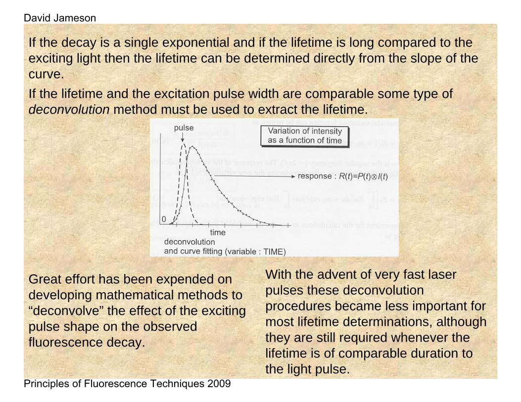
If the decay is a single exponential and if the lifetime is long compared to the exciting light then the lifetime can be determined directly from the slope of the curve. If the lifetime and the excitation pulse width are comparable some type of deconvolution method must be used to extract the lifetime.

Great effort has been expended on developing mathematical methods to “deconvolve” the effect of the exciting pulse shape on the observed fluorescence decay.

With the advent of very fast laser pulses these deconvolutionprocedures became less important for most lifetime determinations, although they are still required whenever the lifetime is of comparable duration to the light pulse.

David Jameson


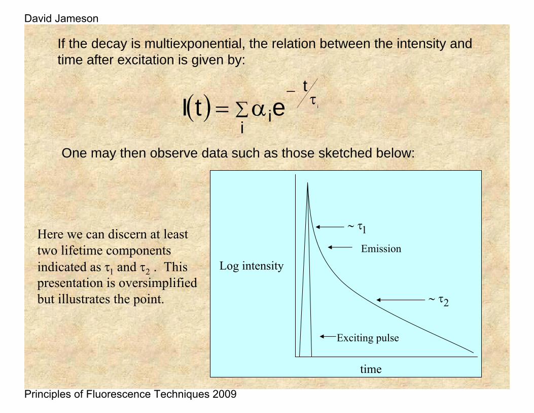
If the decay is multiexponential, the relation between the intensity and time after excitation is given by:

( ) ∑τ−

α=i

t

iietI

One may then observe data such as those sketched below:

time

Log intensity

Exciting pulse

Emission

∼ τ1

∼ τ2

Here we can discern at least two lifetime components indicated as τ1 and τ2 . This presentation is oversimplified but illustrates the point.

David Jameson


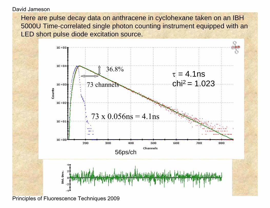
Here are pulse decay data on anthracene in cyclohexane taken on an IBH 5000U Time-correlated single photon counting instrument equipped with an LED short pulse diode excitation source.

τ = 4.1nschi2 = 1.023

56ps/ch

36.8%

73 channels

73 x 0.056ns = 4.1ns

David Jameson


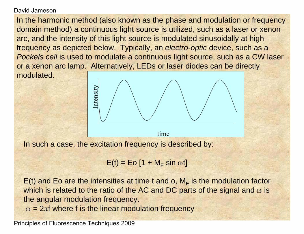
In the harmonic method (also known as the phase and modulation or frequency domain method) a continuous light source is utilized, such as a laser or xenon arc, and the intensity of this light source is modulated sinusoidally at high frequency as depicted below. Typically, an electro-optic device, such as a Pockels cell is used to modulate a continuous light source, such as a CW laser or a xenon arc lamp. Alternatively, LEDs or laser diodes can be directly modulated.

time

Inte

nsity

In such a case, the excitation frequency is described by:

E(t) = Eo [1 + ME sin ωt]

E(t) and Eo are the intensities at time t and o, ME is the modulation factor which is related to the ratio of the AC and DC parts of the signal and ω is the angular modulation frequency.ω = 2πf where f is the linear modulation frequency

David Jameson


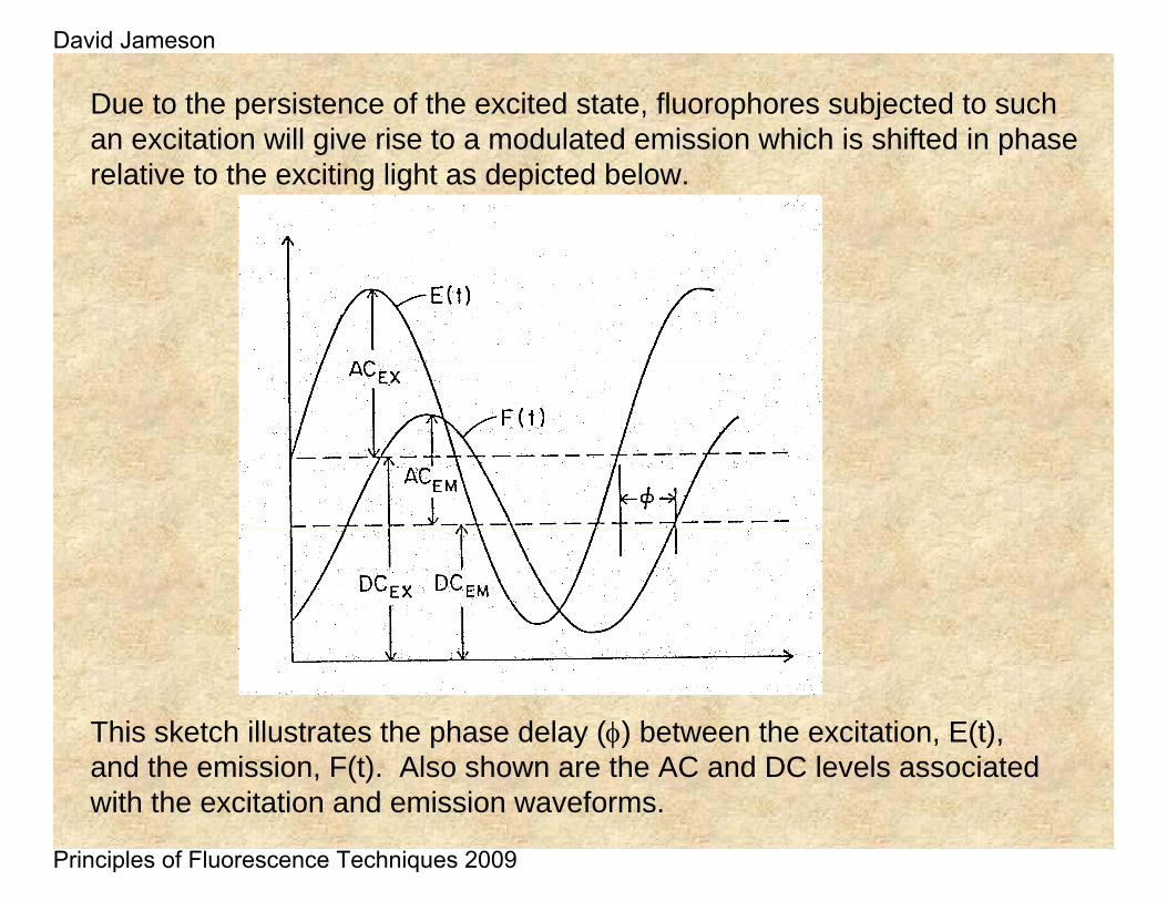
Due to the persistence of the excited state, fluorophores subjected to such an excitation will give rise to a modulated emission which is shifted in phase relative to the exciting light as depicted below.

This sketch illustrates the phase delay (φ) between the excitation, E(t), and the emission, F(t). Also shown are the AC and DC levels associated with the excitation and emission waveforms.

David Jameson


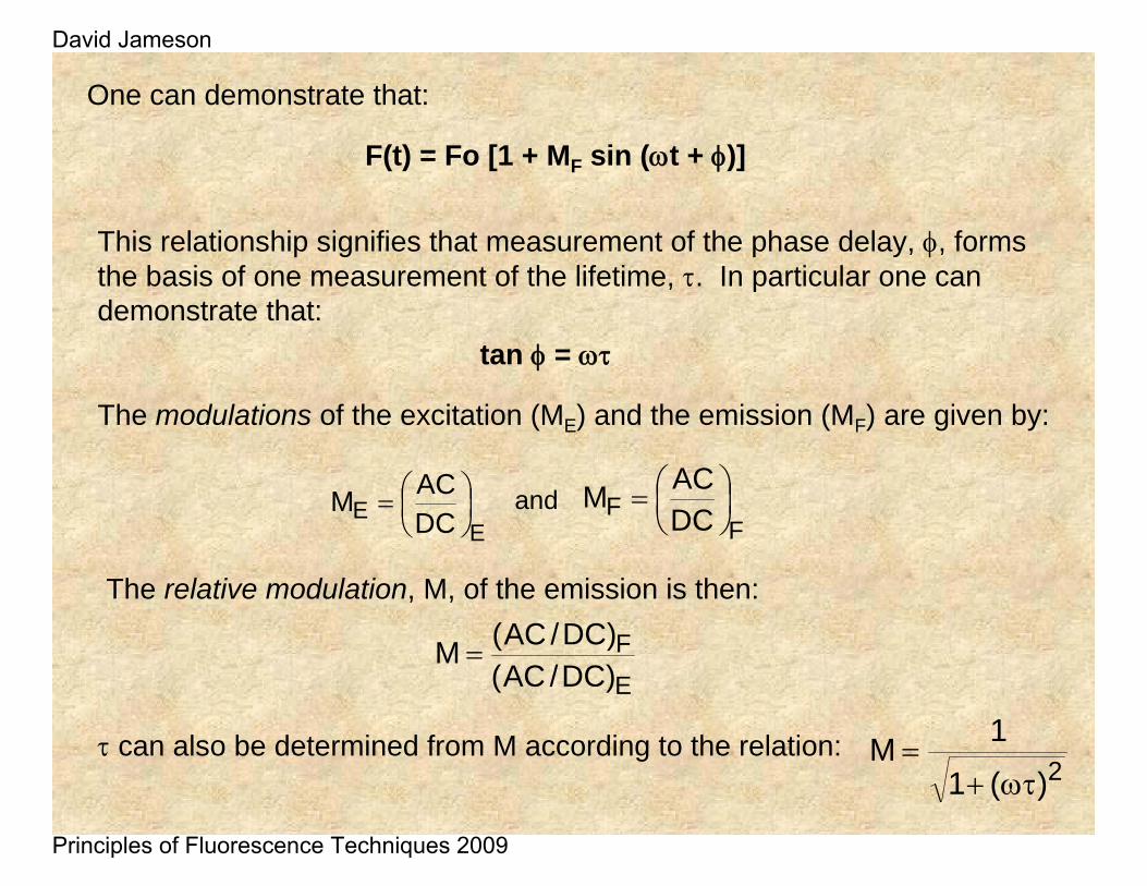
One can demonstrate that:

This relationship signifies that measurement of the phase delay, φ, forms the basis of one measurement of the lifetime, τ. In particular one can demonstrate that:

F(t) = Fo [1 + MF sin (ωt + φ)]

tan φ = ωτ

The modulations of the excitation (ME) and the emission (MF) are given by:

EE DC

ACM ⎟⎠⎞

⎜⎝⎛=

FF DC

ACM ⎟⎠⎞

⎜⎝⎛=and

The relative modulation, M, of the emission is then:

EF

)DC/AC()DC/AC(M =

τ can also be determined from M according to the relation:2)(1

1Mωτ+

=

David Jameson


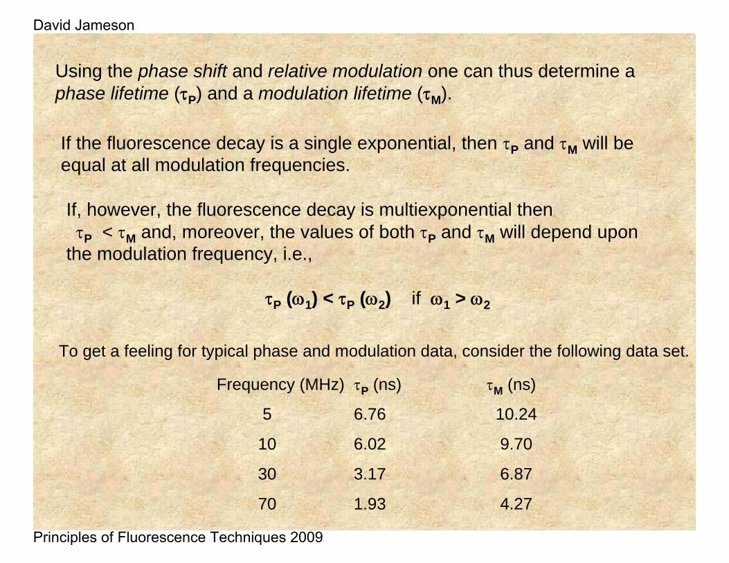
Using the phase shift and relative modulation one can thus determine a phase lifetime (τP) and a modulation lifetime (τM).

If the fluorescence decay is a single exponential, then τP and τM will be equal at all modulation frequencies.

If, however, the fluorescence decay is multiexponential then τP < τM and, moreover, the values of both τP and τM will depend upon

the modulation frequency, i.e.,

τP (ω1) < τP (ω2) if ω1 > ω2

Frequency (MHz) τP (ns) τM (ns)

5 6.76 10.24

10 6.02 9.70

30 3.17 6.87

70 1.93 4.27

To get a feeling for typical phase and modulation data, consider the following data set.

David Jameson


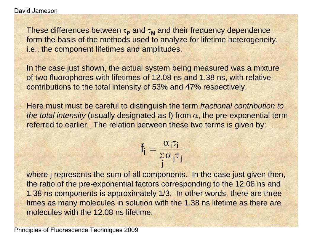
These differences between τP and τM and their frequency dependence form the basis of the methods used to analyze for lifetime heterogeneity, i.e., the component lifetimes and amplitudes.

In the case just shown, the actual system being measured was a mixture of two fluorophores with lifetimes of 12.08 ns and 1.38 ns, with relative contributions to the total intensity of 53% and 47% respectively.

Here must must be careful to distinguish the term fractional contribution to the total intensity (usually designated as f) from α, the pre-exponential term referred to earlier. The relation between these two terms is given by:

∑ τατα=

jjj

iiif

where j represents the sum of all components. In the case just given then, the ratio of the pre-exponential factors corresponding to the 12.08 ns and 1.38 ns components is approximately 1/3. In other words, there are three times as many molecules in solution with the 1.38 ns lifetime as there are molecules with the 12.08 ns lifetime.

David Jameson


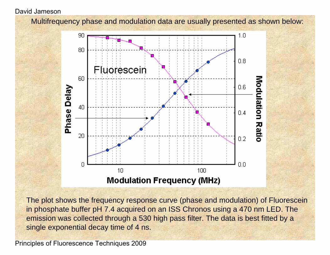
Multifrequency phase and modulation data are usually presented as shown below:

The plot shows the frequency response curve (phase and modulation) of Fluoresceinin phosphate buffer pH 7.4 acquired on an ISS Chronos using a 470 nm LED. The emission was collected through a 530 high pass filter. The data is best fitted by a single exponential decay time of 4 ns.

David Jameson


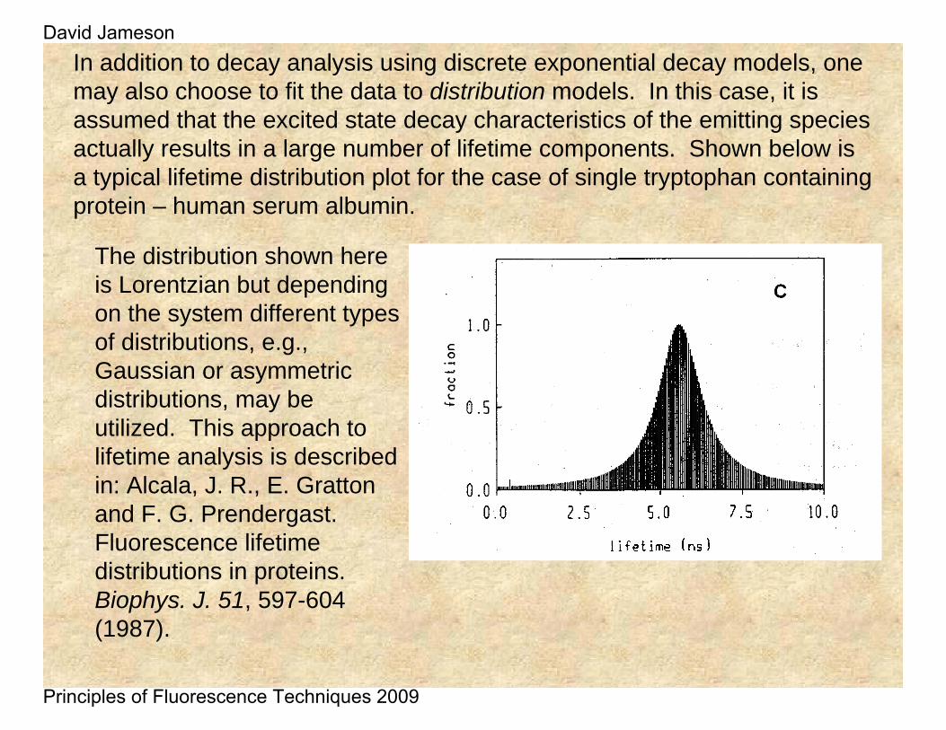
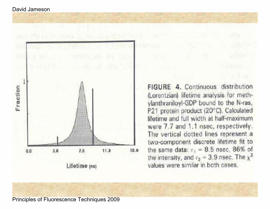
In addition to decay analysis using discrete exponential decay models, one may also choose to fit the data to distribution models. In this case, it is assumed that the excited state decay characteristics of the emitting species actually results in a large number of lifetime components. Shown below is a typical lifetime distribution plot for the case of single tryptophan containing protein – human serum albumin.

The distribution shown here is Lorentzian but depending on the system different types of distributions, e.g., Gaussian or asymmetric distributions, may be utilized. This approach to lifetime analysis is described in: Alcala, J. R., E. Gratton and F. G. Prendergast. Fluorescence lifetime distributions in proteins. Biophys. J. 51, 597-604 (1987).

David Jameson


David Jameson


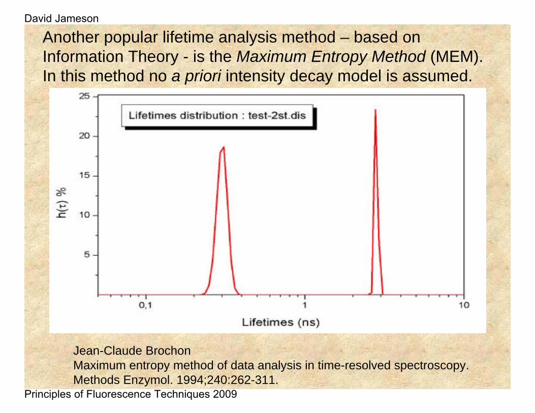
Another popular lifetime analysis method – based on Information Theory - is the Maximum Entropy Method (MEM). In this method no a priori intensity decay model is assumed.

Jean-Claude BrochonMaximum entropy method of data analysis in time-resolved spectroscopy.Methods Enzymol. 1994;240:262-311.

David Jameson


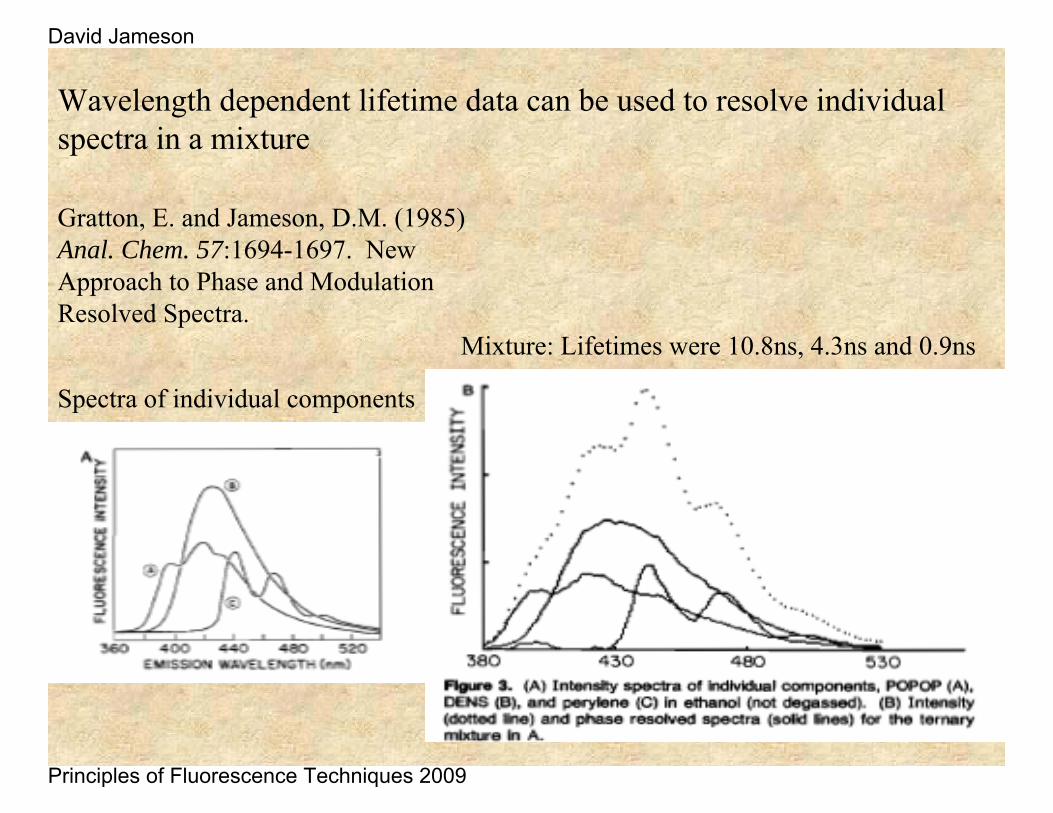
Wavelength dependent lifetime data can be used to resolve individual spectra in a mixture

Gratton, E. and Jameson, D.M. (1985) Anal. Chem. 57:1694-1697. New Approach to Phase and Modulation Resolved Spectra.

Mixture: Lifetimes were 10.8ns, 4.3ns and 0.9ns

Spectra of individual components

David Jameson


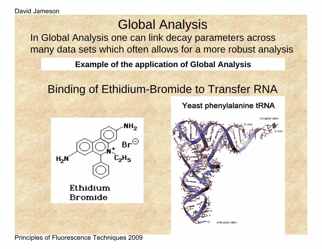
Global AnalysisIn Global Analysis one can link decay parameters across many data sets which often allows for a more robust analysis

Example of the application of Global Analysis

Binding of Ethidium-Bromide to Transfer RNA

David Jameson


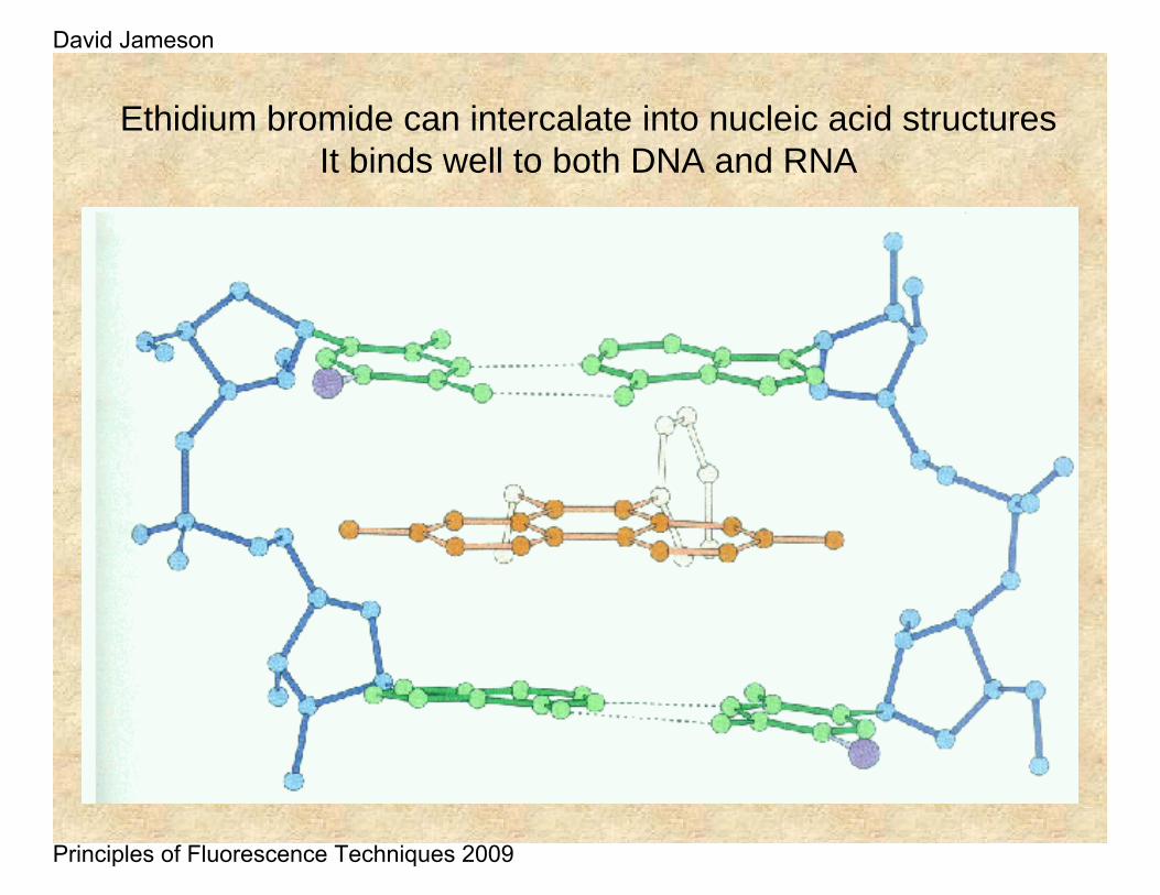
Ethidium bromide can intercalate into nucleic acid structuresIt binds well to both DNA and RNA

David Jameson


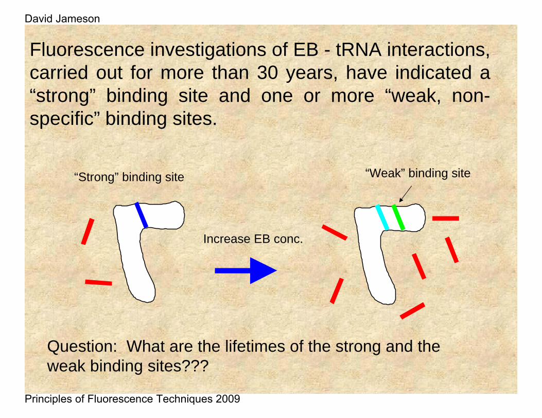
“Strong” binding site

Increase EB conc.

“Weak” binding site

Question: What are the lifetimes of the strong and the weak binding sites???

Fluorescence investigations of EB - tRNA interactions, carried out for more than 30 years, have indicated a “strong” binding site and one or more “weak, non-specific” binding sites.

David Jameson


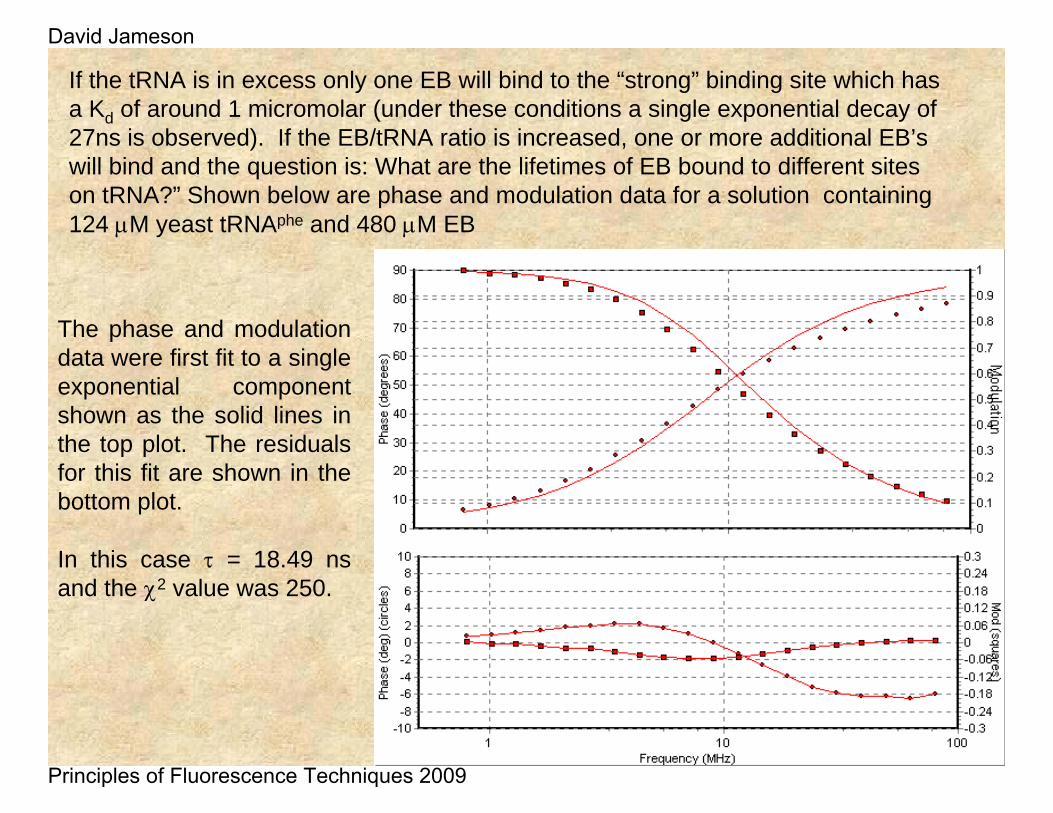
If the tRNA is in excess only one EB will bind to the “strong” binding site which has a Kd of around 1 micromolar (under these conditions a single exponential decay of 27ns is observed). If the EB/tRNA ratio is increased, one or more additional EB’swill bind and the question is: What are the lifetimes of EB bound to different sites on tRNA?” Shown below are phase and modulation data for a solution containing 124 μM yeast tRNAphe and 480 μM EB

The phase and modulation data were first fit to a single exponential component shown as the solid lines in the top plot. The residuals for this fit are shown in the bottom plot.

In this case τ = 18.49 ns and the χ2 value was 250.

David Jameson


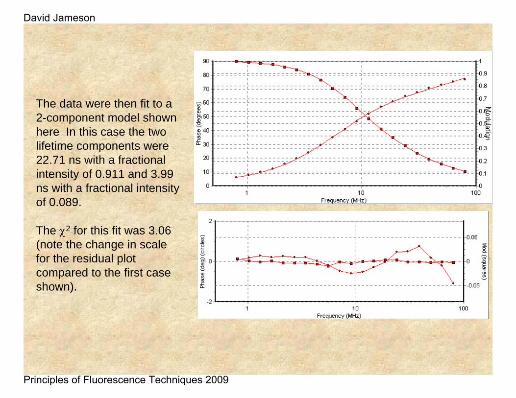
The data were then fit to a 2-component model shown here In this case the two lifetime components were 22.71 ns with a fractional intensity of 0.911 and 3.99 ns with a fractional intensity of 0.089.

The χ2 for this fit was 3.06 (note the change in scale for the residual plot compared to the first case shown).

David Jameson


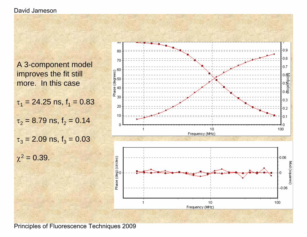
A 3-component model improves the fit still more. In this case

τ1 = 24.25 ns, f1 = 0.83

τ2 = 8.79 ns, f2 = 0.14

τ3 = 2.09 ns, f3 = 0.03

χ2 = 0.39.

David Jameson


Adding a fourth component – with all parameters free to vary - does not lead to a significant improvement in the χ2. In this case one finds 4 components of 24.80 ns (0.776), 12.13ns (0.163), 4.17 ns (0.53) and 0.88 ns (0.008).

But we are not using all of our information! We can actually fix some of the components in this case. We know that free EB has a lifetime of 1.84 ns and we also know that the lifetime of EB bound to the “strong” tRNA binding site is 27 ns. So we can fix these in the analysis. The results are four lifetime components of 27 ns (0.612), 18.33 ns (0.311), 5.85 ns (0.061) and 1.84 ns (0.016). The χ2 improves to 0.16.

We can then go one step better and carry out “Global Analysis”. In Global Analysis, multiple data sets are analyzed simultaneously and different parameters (such as lifetimes) can be “linked” across the data sets. The important concept in this particular experiment is that the lifetimes of the components stay the same and only their fractional contributions change as more ethidioum bromide binds.

David Jameson


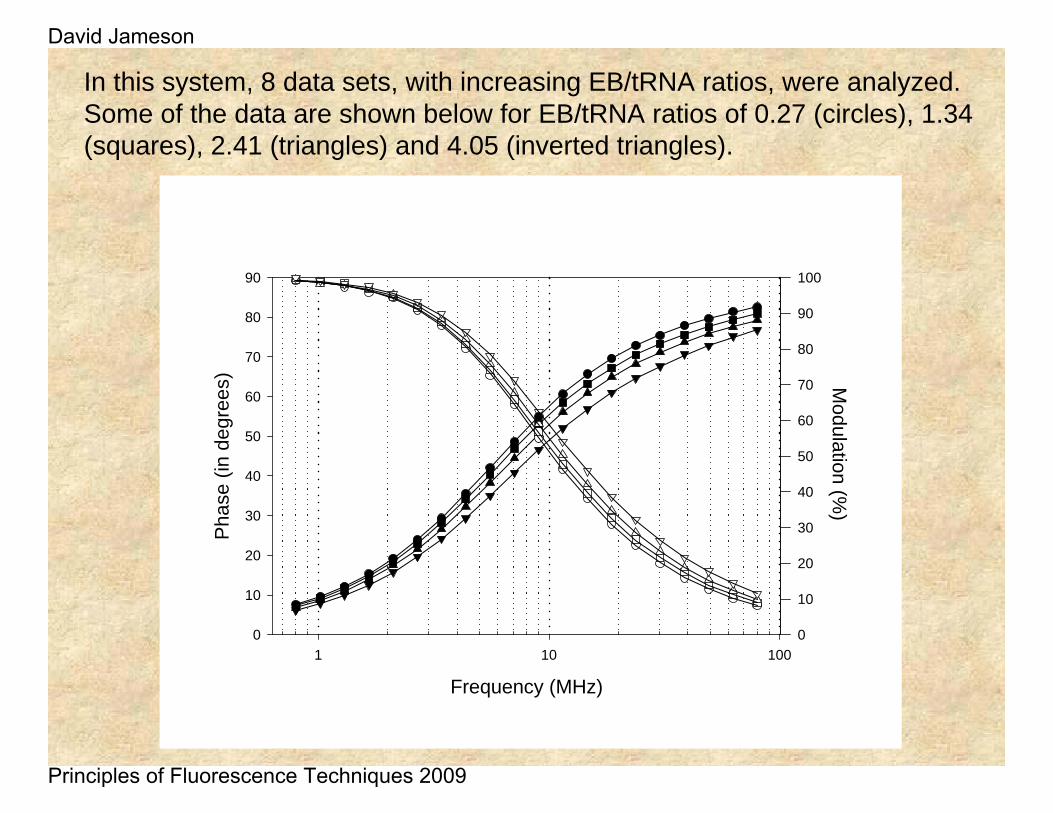
In this system, 8 data sets, with increasing EB/tRNA ratios, were analyzed. Some of the data are shown below for EB/tRNA ratios of 0.27 (circles), 1.34 (squares), 2.41 (triangles) and 4.05 (inverted triangles).

Frequency (MHz)

1 10 100

Pha

se (i

n de

gree

s)

0

10

20

30

40

50

60

70

80

90

Modulation (%

)

0

10

20

30

40

50

60

70

80

90

100

David Jameson


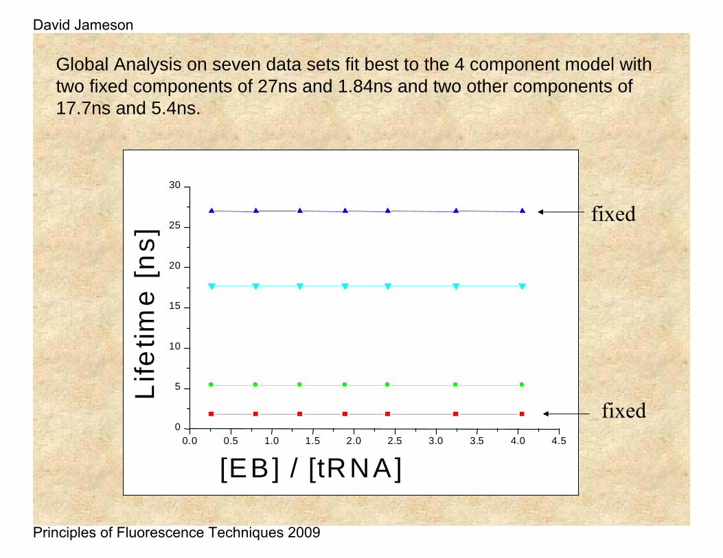
Global Analysis on seven data sets fit best to the 4 component model with two fixed components of 27ns and 1.84ns and two other components of 17.7ns and 5.4ns.

Life

ti me

[ ns]

0.0 0.5 1.0 1.5 2.0 2.5 3.0 3.5 4.0 4.50

5

10

15

20

25

30

[EB] / [tRNA]

fixed

fixed

David Jameson


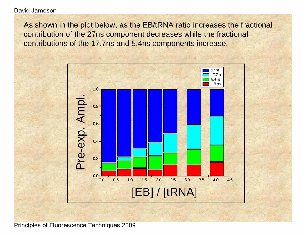
As shown in the plot below, as the EB/tRNA ratio increases the fractional contribution of the 27ns component decreases while the fractional contributions of the 17.7ns and 5.4ns components increase.

0.0 0.5 1.0 1.5 2.0 2.5 3.0 3.5 4.0 4.50.0

0.2

0.4

0.6

0.8

1.0

27 ns17.7 ns5.4 ns1.8 ns

Pre

-ex p

.Am

pl.

[EB] / [tRNA]

David Jameson


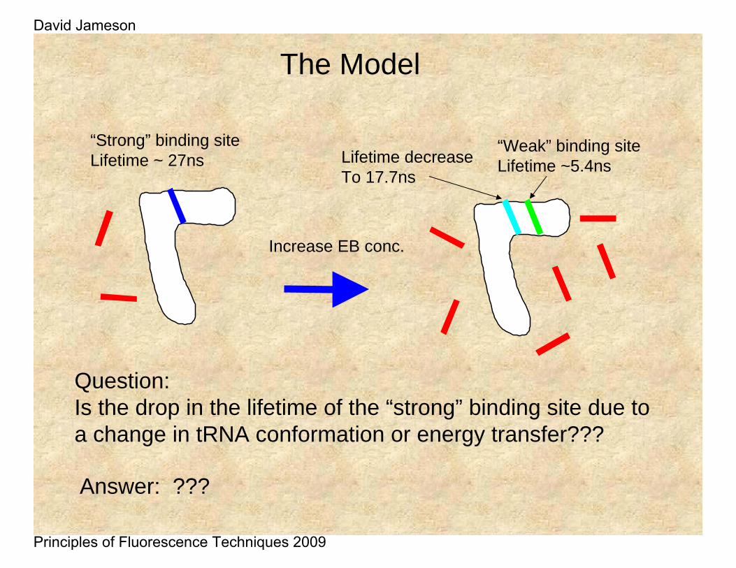
“Strong” binding siteLifetime ~ 27ns

Increase EB conc.

Lifetime decreaseTo 17.7ns

“Weak” binding siteLifetime ~5.4ns

Question:Is the drop in the lifetime of the “strong” binding site due to a change in tRNA conformation or energy transfer???

The Model

Answer: ???

David Jameson


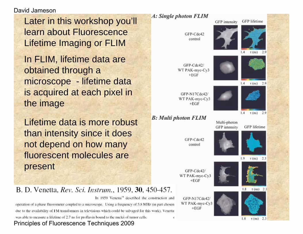
Lifetime data is more robust than intensity since it does not depend on how many fluorescent molecules are present

Later in this workshop you’ll learn about Fluorescence Lifetime Imaging or FLIM

In FLIM, lifetime data are obtained through a microscope - lifetime data is acquired at each pixel in the image

David Jameson


Time-Resolved Anisotropy and Excited State Reactions

Many of these slides were prepared by Theodore Hazlett

David Jameson


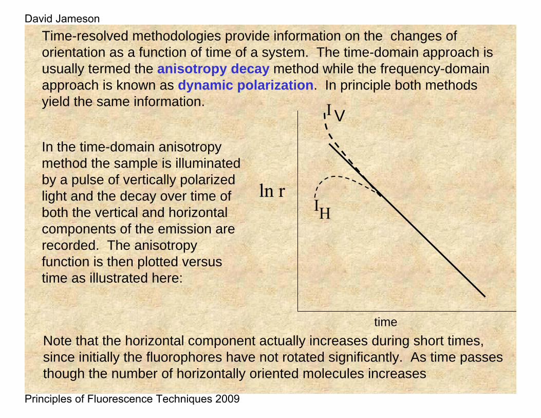
Time-resolved methodologies provide information on the changes of orientation as a function of time of a system. The time-domain approach is usually termed the anisotropy decay method while the frequency-domain approach is known as dynamic polarization. In principle both methods yield the same information.

In the time-domain anisotropy method the sample is illuminated by a pulse of vertically polarized light and the decay over time of both the vertical and horizontal components of the emission are recorded. The anisotropy function is then plotted versus time as illustrated here:

VI

ln r

time

HI

Note that the horizontal component actually increases during short times, since initially the fluorophores have not rotated significantly. As time passes though the number of horizontally oriented molecules increases

David Jameson


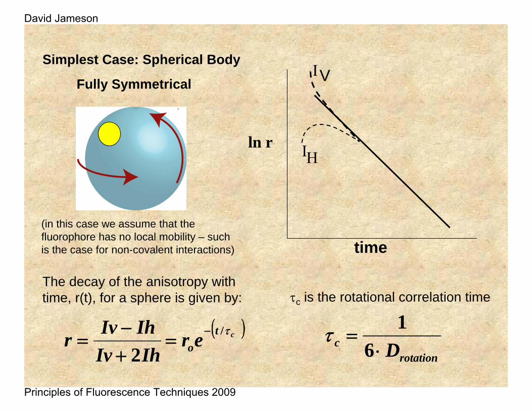
The decay of the anisotropy with time, r(t), for a sphere is given by:

( )ctoer

IhIvIhIvr τ/

2−

=+−

=

VI

ln r

time

HI

Simplest Case: Spherical Body

Fully Symmetrical

rotationc D⋅

=6

1τ

τc is the rotational correlation time

(in this case we assume that the fluorophore has no local mobility – such is the case for non-covalent interactions)

David Jameson


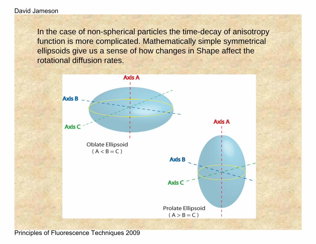
In the case of non-spherical particles the time-decay of anisotropy function is more complicated. Mathematically simple symmetrical ellipsoids give us a sense of how changes in Shape affect the rotational diffusion rates.

David Jameson


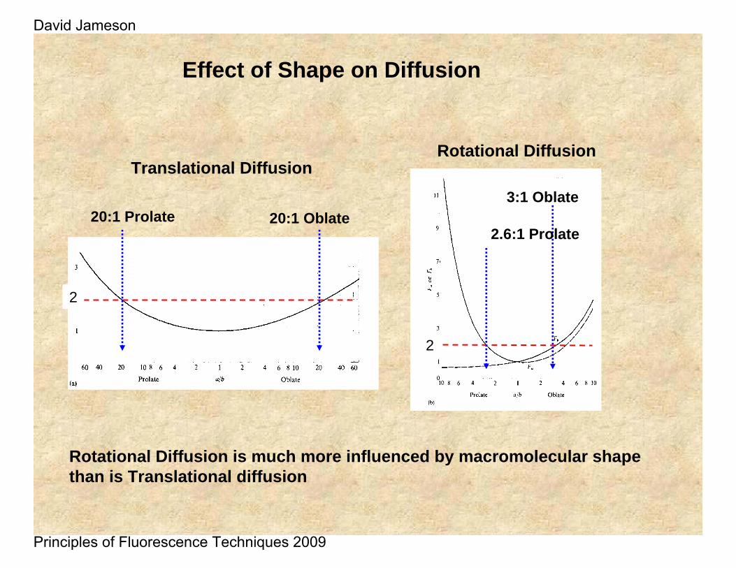
Effect of Shape on Diffusion

Rotational Diffusion is much more influenced by macromolecular shape than is Translational diffusion

Translational Diffusion

20:1 Prolate 20:1 Oblate

2

Rotational Diffusion

2

2.6:1 Prolate

3:1 Oblate

David Jameson


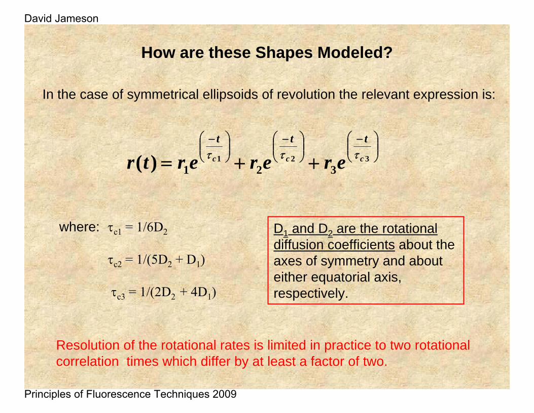
In the case of symmetrical ellipsoids of revolution the relevant expression is:

⎟⎟⎠

⎞⎜⎜⎝

⎛ −⎟⎟⎠

⎞⎜⎜⎝

⎛ −⎟⎟⎠

⎞⎜⎜⎝

⎛ −

++= 321321)( ccc

ttt

ererertr τττ

Resolution of the rotational rates is limited in practice to two rotational correlation times which differ by at least a factor of two.

where: τc1 = 1/6D2

τc2 = 1/(5D2 + D1)

τc3 = 1/(2D2 + 4D1)

D1 and D2 are the rotational diffusion coefficients about the axes of symmetry and about either equatorial axis, respectively.

How are these Shapes Modeled?

David Jameson


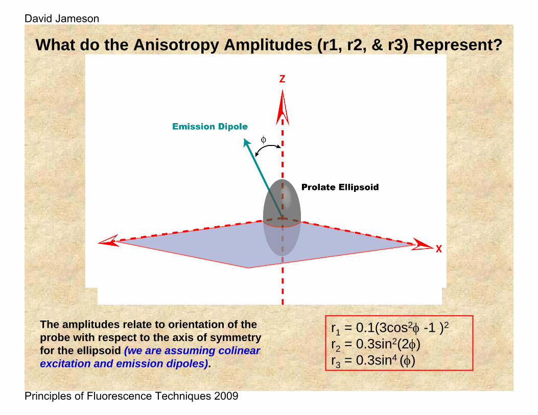
What do the Anisotropy Amplitudes (r1, r2, & r3) Represent?

r1 = 0.1(3cos2φ -1 )2

r2 = 0.3sin2(2φ)r3 = 0.3sin4 (φ)

The amplitudes relate to orientation of the probe with respect to the axis of symmetry for the ellipsoid (we are assuming colinearexcitation and emission dipoles).

David Jameson


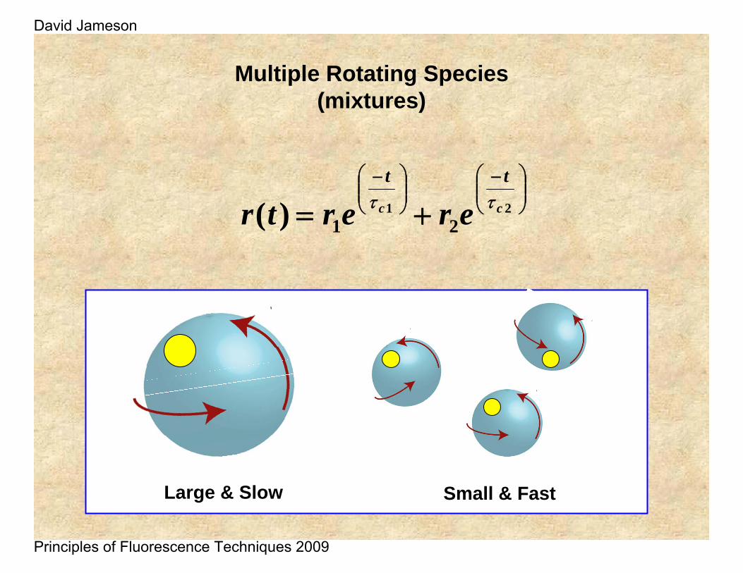
Large & Slow Small & Fast

Multiple Rotating Species(mixtures)

⎟⎟⎠

⎞⎜⎜⎝

⎛ −⎟⎟⎠

⎞⎜⎜⎝

⎛ −

+= 2121)( cc

tt

erertr ττ

David Jameson


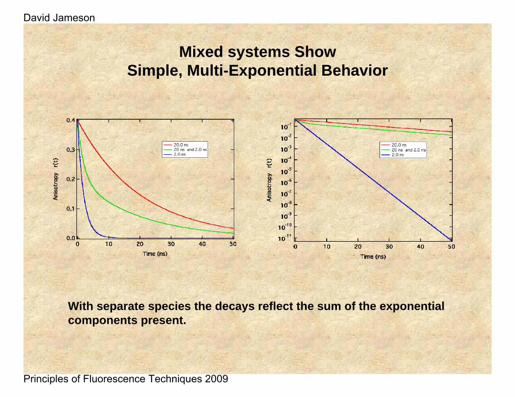
Mixed systems ShowSimple, Multi-Exponential Behavior

With separate species the decays reflect the sum of the exponential components present.

David Jameson


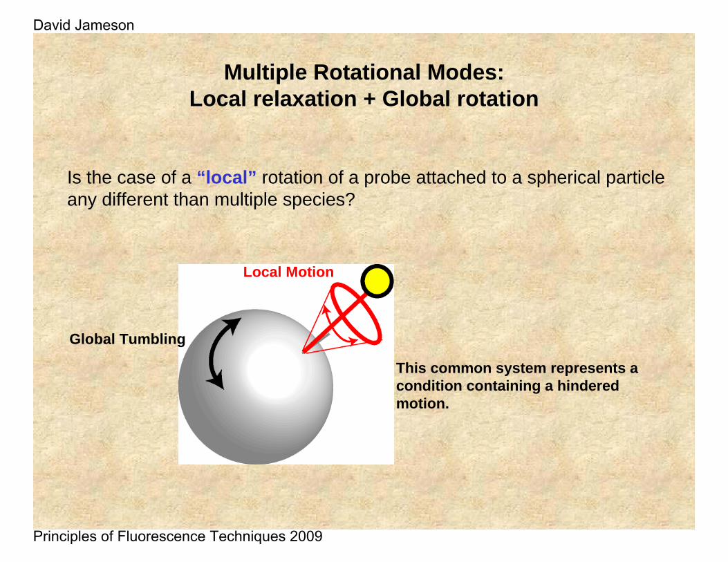
Is the case of a “local” rotation of a probe attached to a spherical particle any different than multiple species?

Multiple Rotational Modes: Local relaxation + Global rotation

This common system represents a condition containing a hindered motion.

Global Tumbling

Local Motion

David Jameson


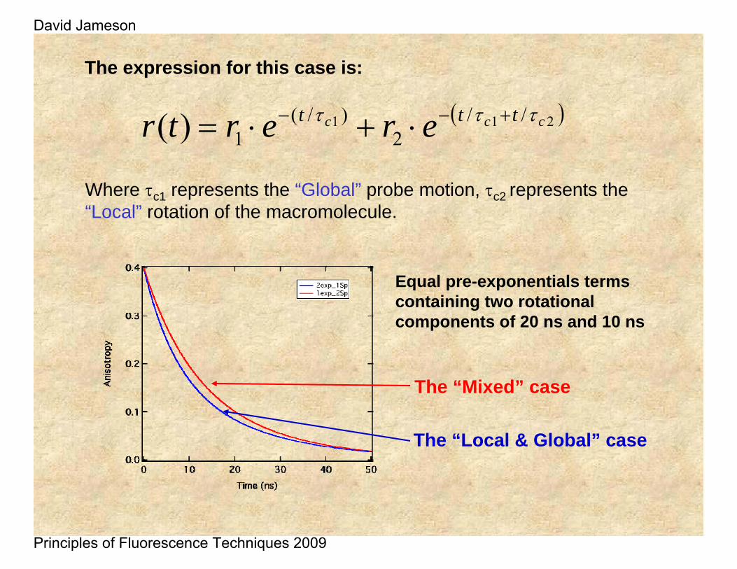
( )211 //2

)/(1)( ccc ttt erertr τττ +−− ⋅+⋅=

Where τc1 represents the “Global” probe motion, τc2 represents the “Local” rotation of the macromolecule.

The expression for this case is:

Equal pre-exponentials terms containing two rotational components of 20 ns and 10 ns

The “Mixed” case

The “Local & Global” case

David Jameson


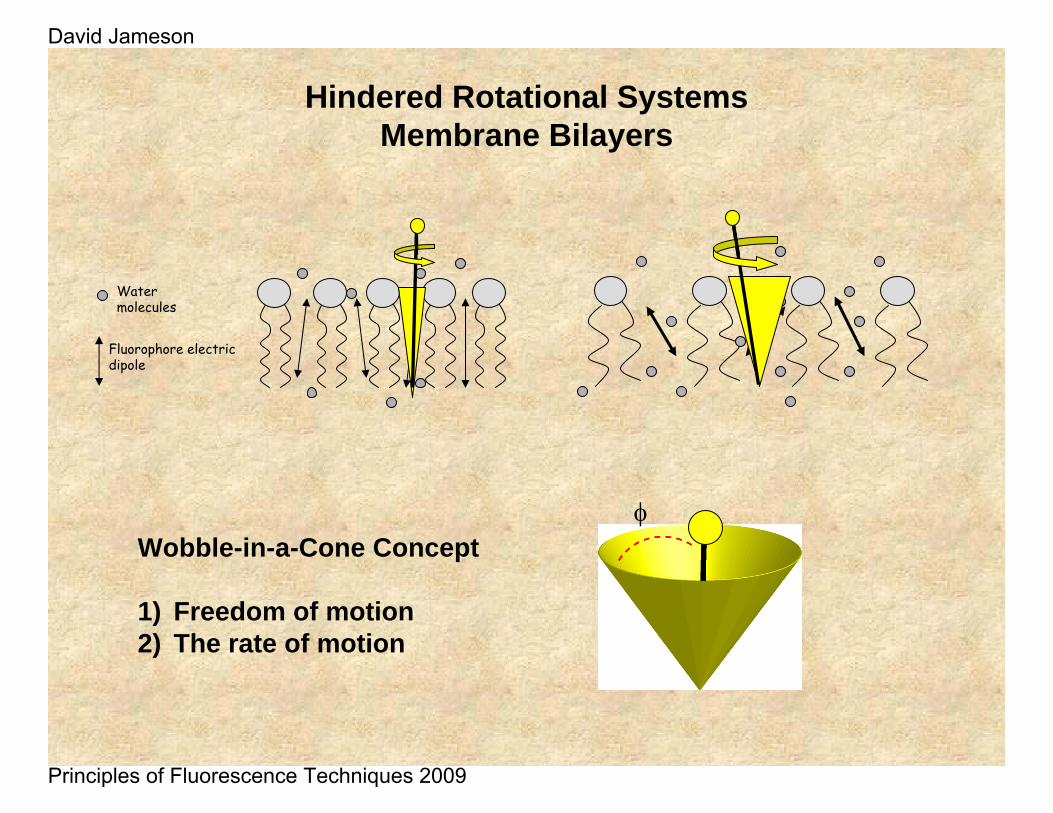
Hindered Rotational SystemsMembrane Bilayers

Fluorophore electric dipole

Water molecules

Wobble-in-a-Cone Concept

1) Freedom of motion2) The rate of motion

φ

David Jameson


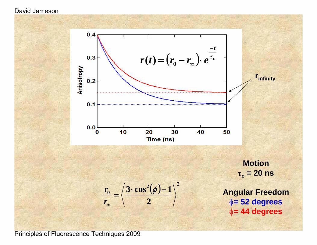
Motionτc = 20 ns

Angular Freedomφ= 52 degreesφ= 44 degrees

rinfinity

( ) 220

21cos3 −⋅

=∞

φrr

( ) c

t

errtr τ−

∞ ⋅−= 0)(

David Jameson


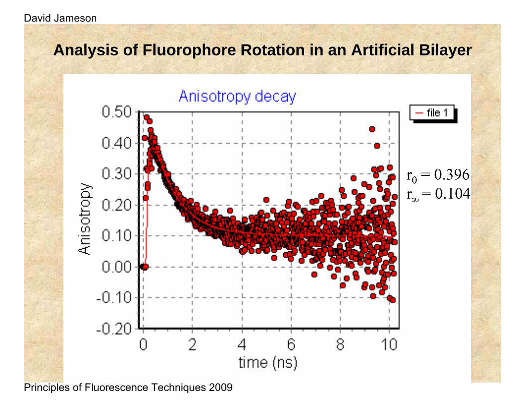
Analysis of Fluorophore Rotation in an Artificial Bilayer

r0 = 0.396r∞ = 0.104

David Jameson


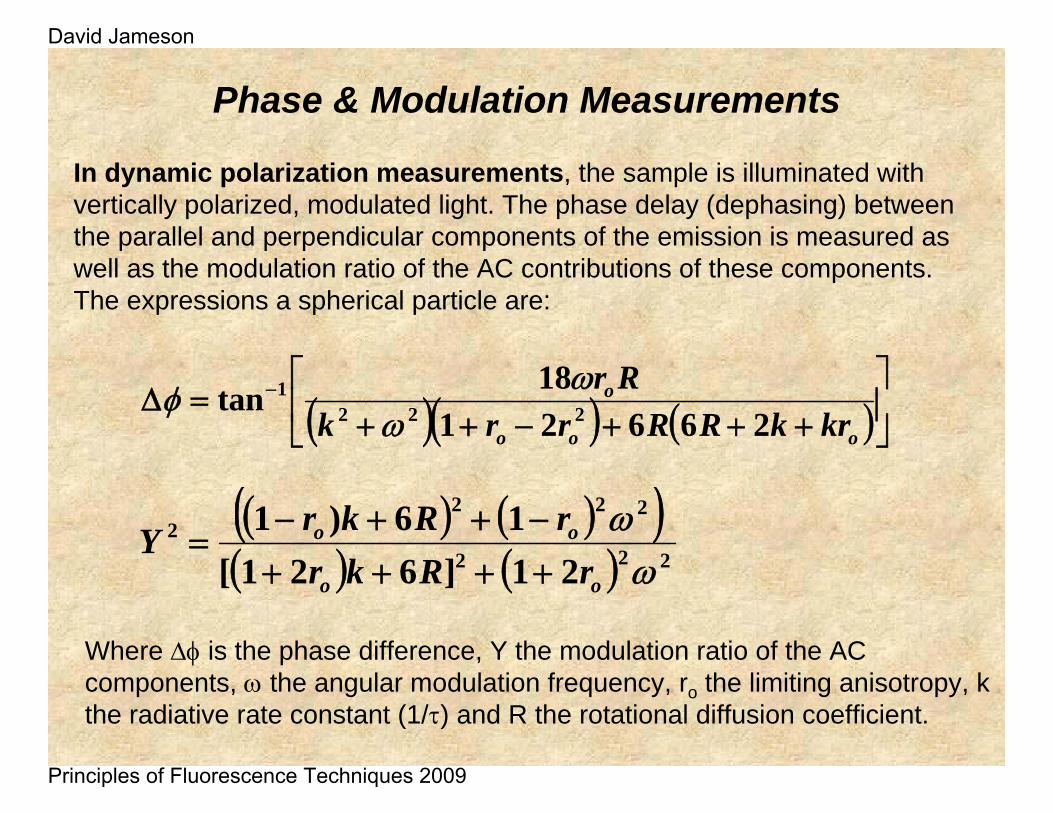
In dynamic polarization measurements, the sample is illuminated with vertically polarized, modulated light. The phase delay (dephasing) between the parallel and perpendicular components of the emission is measured as well as the modulation ratio of the AC contributions of these components. The expressions a spherical particle are:

Phase & Modulation Measurements

( )( ) ( )⎥⎦

⎤⎢⎣

⎡+++−++

=Δ −

ooo

o

krkRRrrkRr

2662118tan 222

1

ωωφ

( ) ( )( )( ) ( ) 222

2222

21]621[16)1

ωω

oo

oo

rRkrrRkrY

++++−++−

=

Where Δφ is the phase difference, Y the modulation ratio of the AC components, ω the angular modulation frequency, ro the limiting anisotropy, k the radiative rate constant (1/τ) and R the rotational diffusion coefficient.

David Jameson


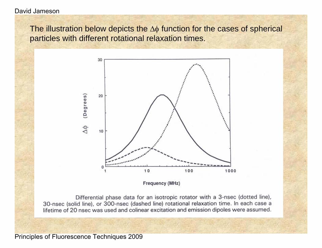
The illustration below depicts the Δφ function for the cases of spherical particles with different rotational relaxation times.

David Jameson


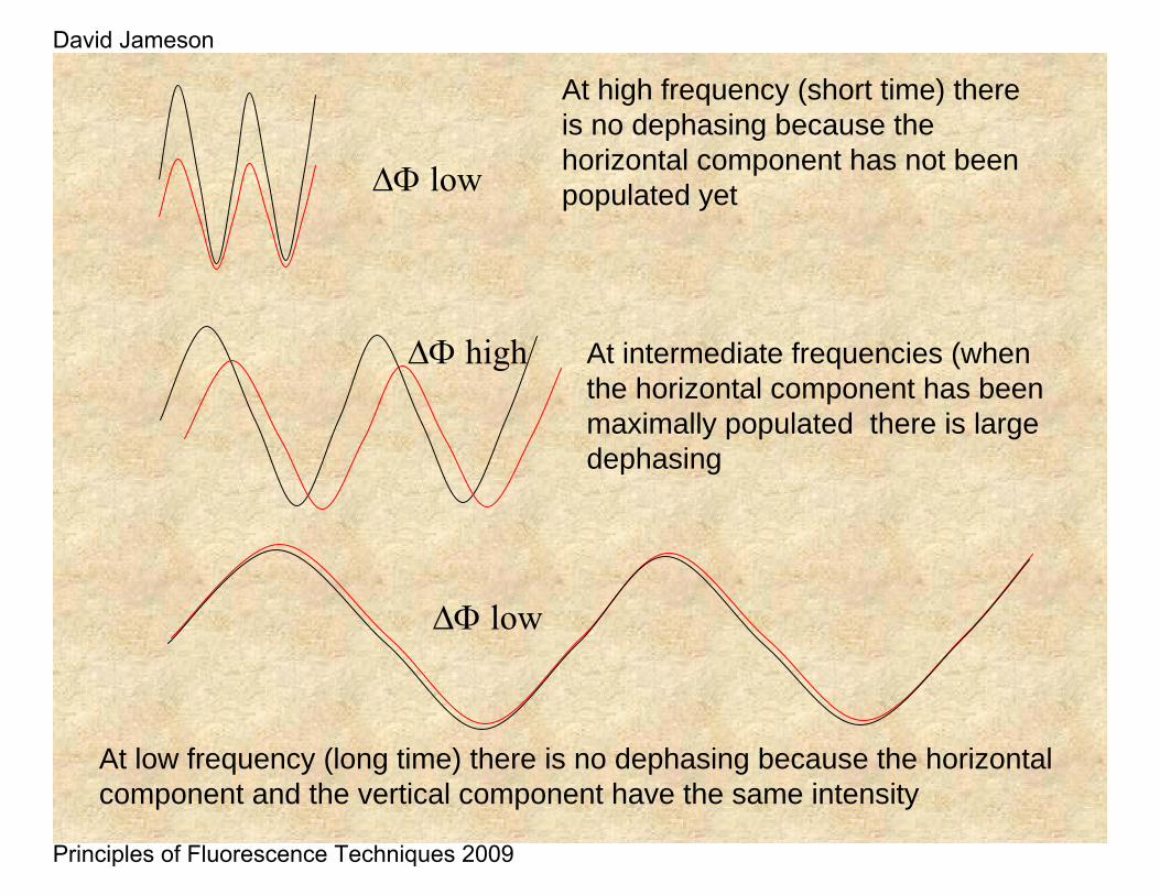
At high frequency (short time) there is no dephasing because the horizontal component has not been populated yet

At low frequency (long time) there is no dephasing because the horizontal component and the vertical component have the same intensity

At intermediate frequencies (when the horizontal component has been maximally populated there is large dephasing

ΔΦ low

ΔΦ high

ΔΦ low

David Jameson


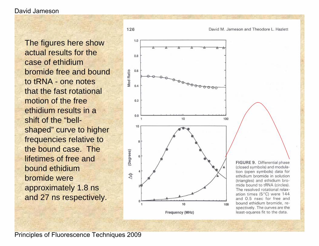
The figures here show actual results for the case of ethidiumbromide free and bound to tRNA - one notes that the fast rotational motion of the free ethidium results in a shift of the “bell-shaped” curve to higher frequencies relative to the bound case. The lifetimes of free and bound ethidiumbromide were approximately 1.8 ns and 27 ns respectively.

David Jameson


0

0.05

0.1

0.15

0.2

0.25

0.3

0.35

0.4

0.45

0.5

0

1

2

3

4

5

6

1 2 4 8 16 32 64 128 256 512

Mod

ulation Ratio

Phase Delay (d

eg)

Frequency (MHz)

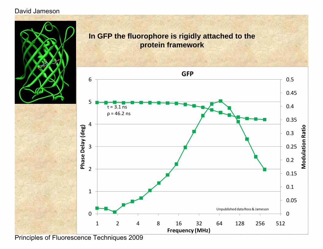
GFP

τ = 3.1 nsρ = 46.2 ns

Unpublished data Ross & Jameson

In GFP the fluorophore is rigidly attached to the protein framework

David Jameson


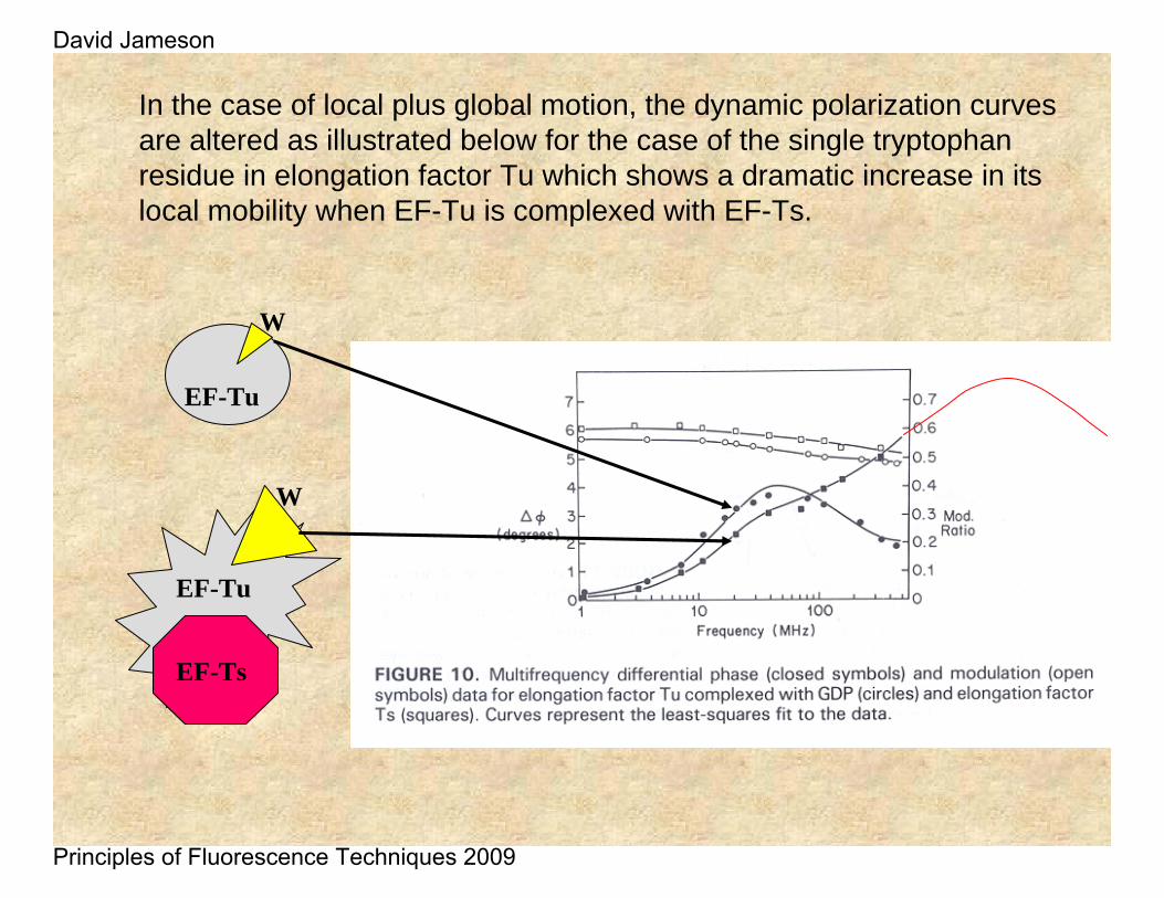
In the case of local plus global motion, the dynamic polarization curves are altered as illustrated below for the case of the single tryptophan residue in elongation factor Tu which shows a dramatic increase in its local mobility when EF-Tu is complexed with EF-Ts.

EF-Tu

W

EF-Tu

EF-Ts

W

David Jameson


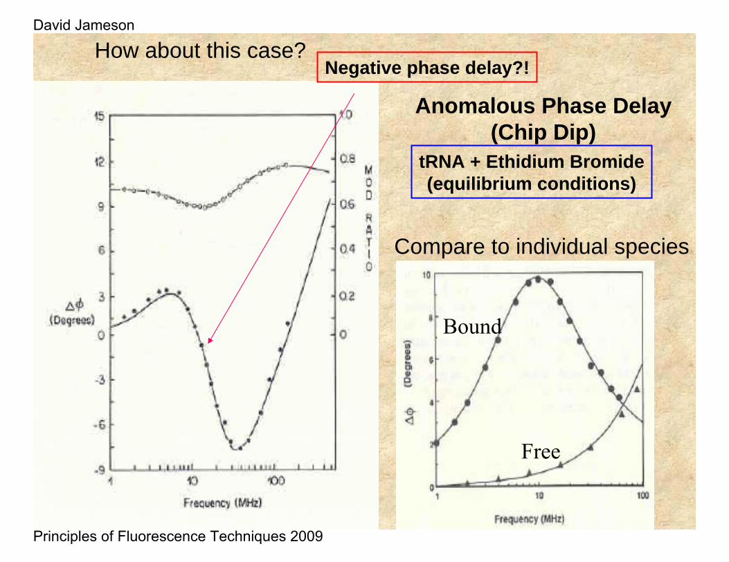
Anomalous Phase Delay(Chip Dip)

tRNA + Ethidium Bromide(equilibrium conditions)

How about this case?Negative phase delay?!

Compare to individual species

Free

Bound

David Jameson


+

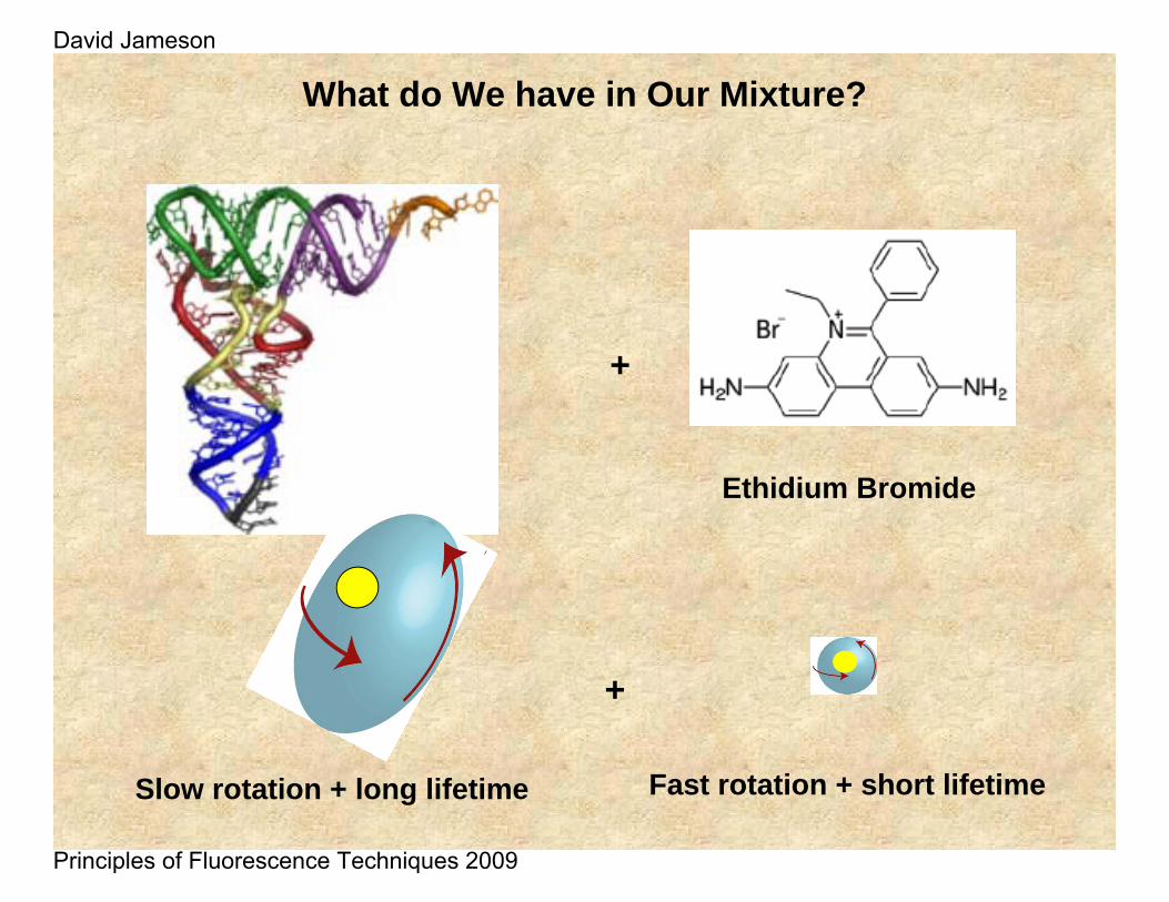
What do We have in Our Mixture?

+

Ethidium Bromide

Slow rotation + long lifetime Fast rotation + short lifetime

David Jameson


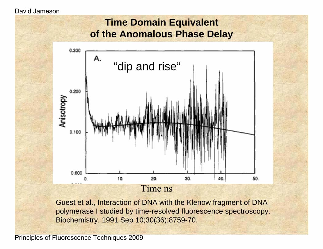
Time Domain Equivalent of the Anomalous Phase Delay

Guest et al., Interaction of DNA with the Klenow fragment of DNA polymerase I studied by time-resolved fluorescence spectroscopy.Biochemistry. 1991 Sep 10;30(36):8759-70.

Time ns

“dip and rise”

David Jameson


0.0

0.2

0.4

0.6

0.8

1.0

0 40 80 120 1600.0

0.2

0.4

0.6

0.8

1.0

Rotational Correlation Time (ns)

Rel

ativ

e A

mpl

itude

(a)

NN

CC

dye(c)

(b)

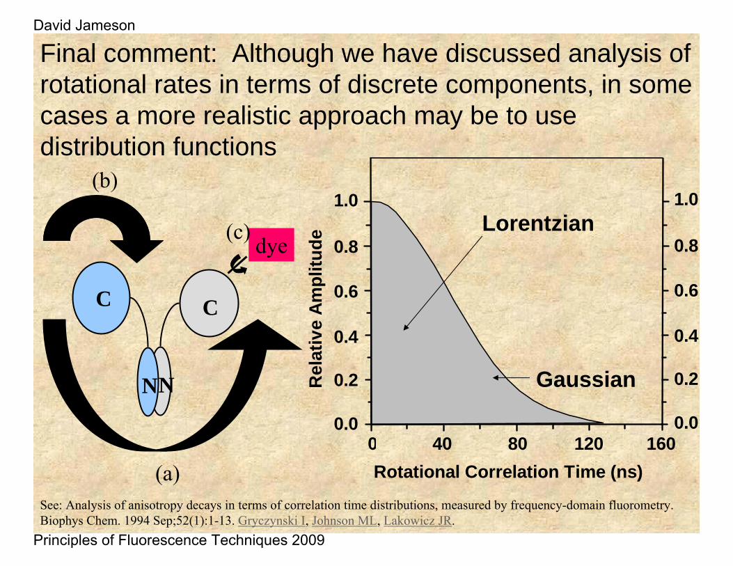
Final comment: Although we have discussed analysis of rotational rates in terms of discrete components, in some cases a more realistic approach may be to use distribution functions

Lorentzian

Gaussian

See: Analysis of anisotropy decays in terms of correlation time distributions, measured by frequency-domain fluorometry. Biophys Chem. 1994 Sep;52(1):1-13. Gryczynski I, Johnson ML, Lakowicz JR.

David Jameson


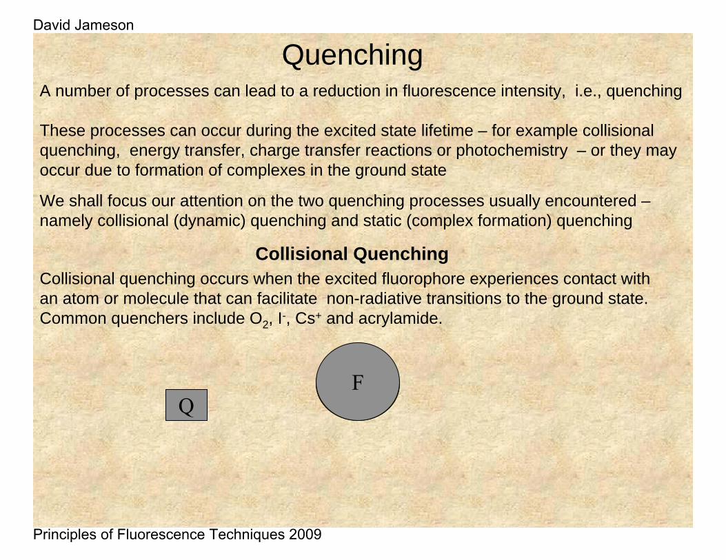
QuenchingA number of processes can lead to a reduction in fluorescence intensity, i.e., quenching

These processes can occur during the excited state lifetime – for example collisional quenching, energy transfer, charge transfer reactions or photochemistry – or they may occur due to formation of complexes in the ground state

We shall focus our attention on the two quenching processes usually encountered –namely collisional (dynamic) quenching and static (complex formation) quenching

Collisional QuenchingCollisional quenching occurs when the excited fluorophore experiences contact with an atom or molecule that can facilitate non-radiative transitions to the ground state. Common quenchers include O2, I-, Cs+ and acrylamide.

F*Q

F

David Jameson


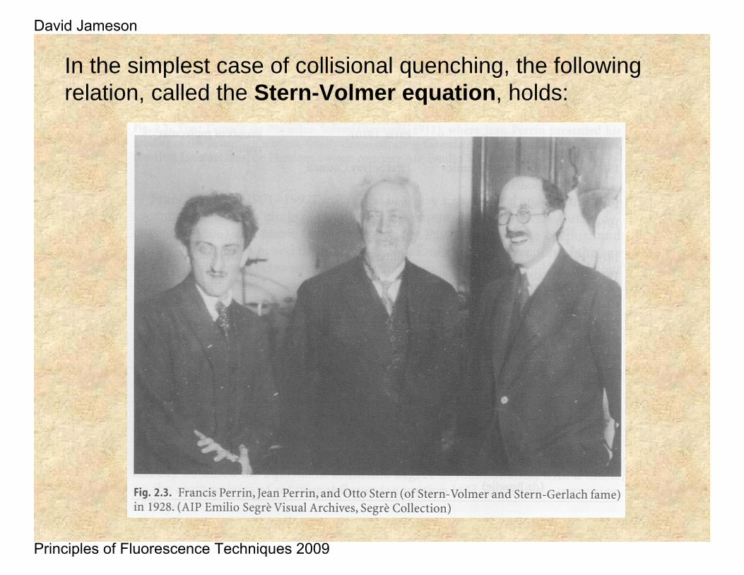
In the simplest case of collisional quenching, the following relation, called the Stern-Volmer equation, holds:

David Jameson


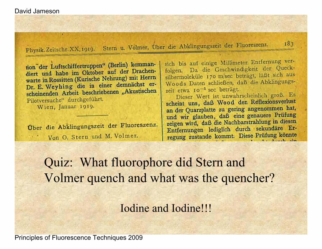
Quiz: What fluorophore did Stern and Volmer quench and what was the quencher?

Iodine and Iodine!!!

David Jameson


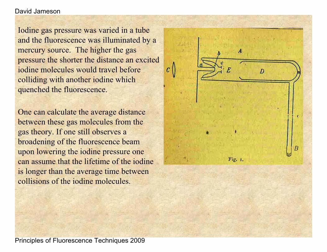
Iodine gas pressure was varied in a tube and the fluorescence was illuminated by a mercury source. The higher the gas pressure the shorter the distance an excited iodine molecules would travel before colliding with another iodine which quenched the fluorescence.

One can calculate the average distance between these gas molecules from the gas theory. If one still observes a broadening of the fluorescence beam upon lowering the iodine pressure one can assume that the lifetime of the iodine is longer than the average time between collisions of the iodine molecules.

David Jameson


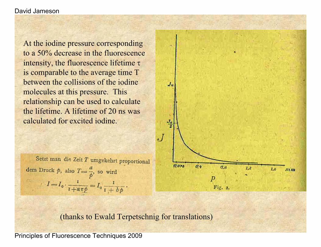
At the iodine pressure corresponding to a 50% decrease in the fluorescence intensity, the fluorescence lifetime τis comparable to the average time T between the collisions of the iodine molecules at this pressure. This relationship can be used to calculate the lifetime. A lifetime of 20 ns was calculated for excited iodine.

(thanks to Ewald Terpetschnig for translations)

David Jameson


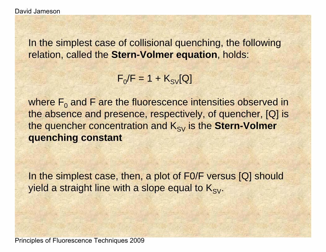
In the simplest case of collisional quenching, the following relation, called the Stern-Volmer equation, holds:

F0/F = 1 + KSV[Q]

where F0 and F are the fluorescence intensities observed in the absence and presence, respectively, of quencher, [Q] is the quencher concentration and KSV is the Stern-Volmer quenching constant

In the simplest case, then, a plot of F0/F versus [Q] should yield a straight line with a slope equal to KSV.

David Jameson


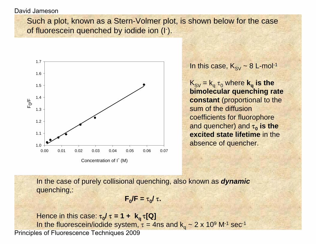
Such a plot, known as a Stern-Volmer plot, is shown below for the case of fluorescein quenched by iodide ion (I-).

Concentration of I- (M)

0.00 0.01 0.02 0.03 0.04 0.05 0.06 0.07

F 0/F

1.0

1.1

1.2

1.3

1.4

1.5

1.6

1.7

In the case of purely collisional quenching, also known as dynamicquenching,:

F0/F = τ0/ τ.

Hence in this case: τ0/ τ = 1 + kq τ[Q] In the fluorescein/iodide system, τ = 4ns and kq ~ 2 x 109 M-1 sec-1

In this case, KSV ~ 8 L-mol-1

KSV = kq τ0 where kq is the bimolecular quenching rate constant (proportional to the sum of the diffusion coefficients for fluorophore and quencher) and τ0 is the excited state lifetime in the absence of quencher.

David Jameson


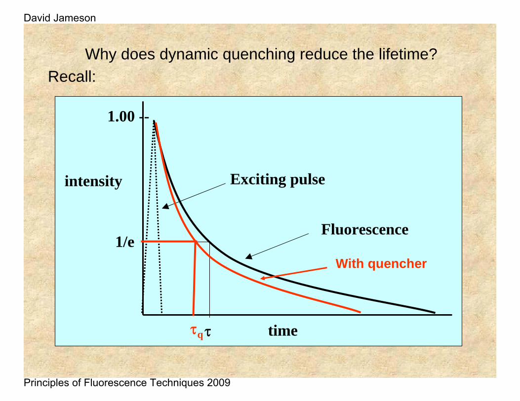
Why does dynamic quenching reduce the lifetime?Recall:

time

intensity

1.00 --

1/e

Exciting pulse

Fluorescence

ττq

With quencher

David Jameson


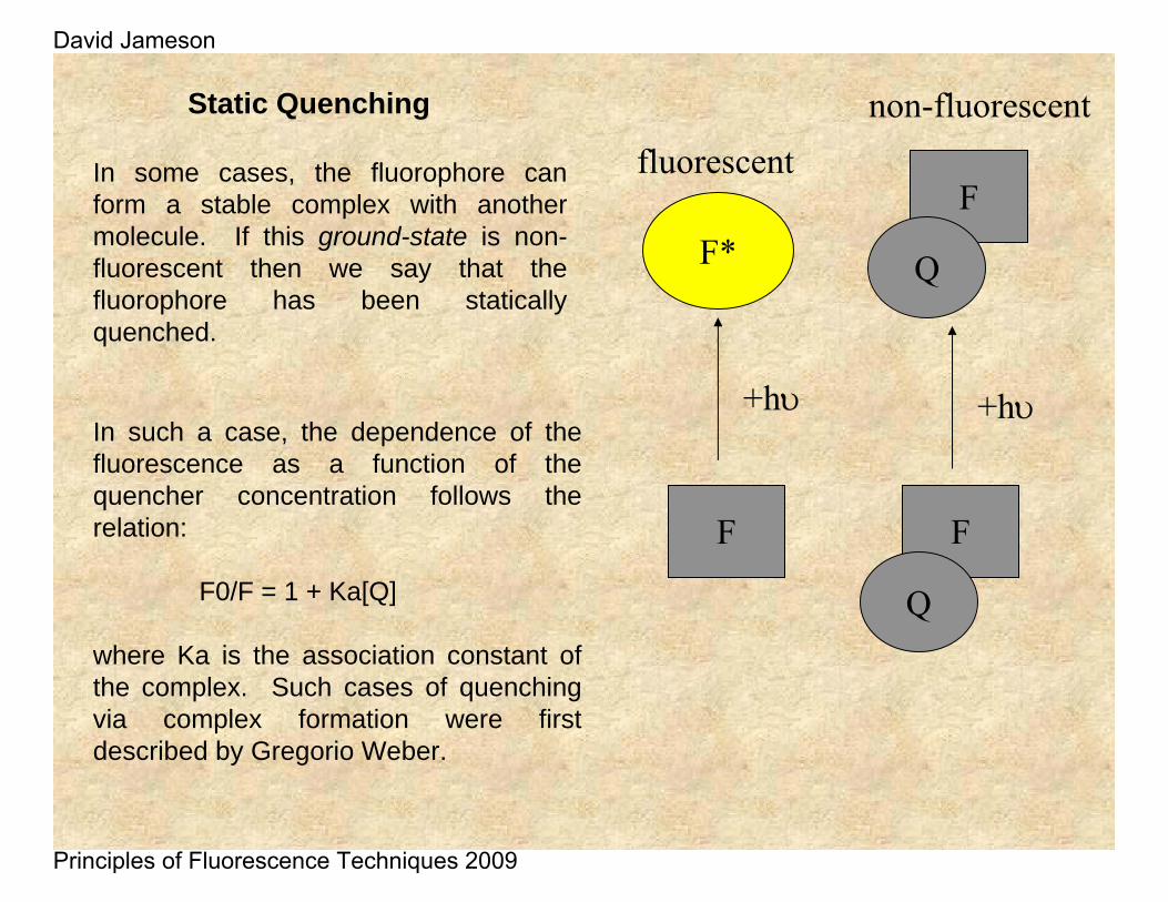
Static Quenching

In some cases, the fluorophore can form a stable complex with another molecule. If this ground-state is non-fluorescent then we say that the fluorophore has been statically quenched.

F

F*

+hυ

fluorescent

F

Q

+hυ

F

Q

non-fluorescent

In such a case, the dependence of the fluorescence as a function of the quencher concentration follows the relation:

F0/F = 1 + Ka[Q]

where Ka is the association constant of the complex. Such cases of quenching via complex formation were first described by Gregorio Weber.

David Jameson


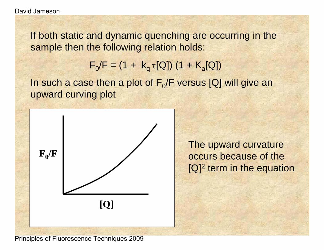
F0/F

[Q]

The upward curvature occurs because of the [Q]2 term in the equation

If both static and dynamic quenching are occurring in the sample then the following relation holds:

F0/F = (1 + kq τ[Q]) (1 + Ka[Q])

In such a case then a plot of F0/F versus [Q] will give an upward curving plot

David Jameson


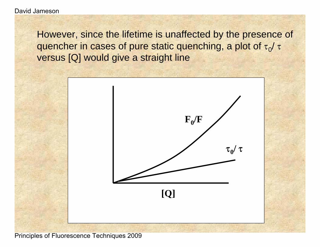
However, since the lifetime is unaffected by the presence of quencher in cases of pure static quenching, a plot of τ0/ τversus [Q] would give a straight line

F0/F

[Q]

τ0/ τ

David Jameson


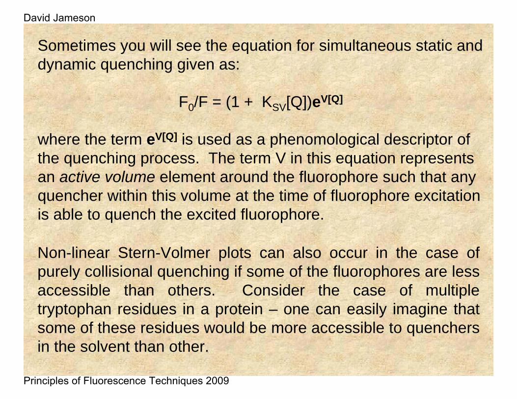
Sometimes you will see the equation for simultaneous static and dynamic quenching given as:

F0/F = (1 + KSV[Q])eV[Q]

where the term eV[Q] is used as a phenomological descriptor of the quenching process. The term V in this equation represents an active volume element around the fluorophore such that any quencher within this volume at the time of fluorophore excitation is able to quench the excited fluorophore.

Non-linear Stern-Volmer plots can also occur in the case of purely collisional quenching if some of the fluorophores are less accessible than others. Consider the case of multiple tryptophan residues in a protein – one can easily imagine that some of these residues would be more accessible to quenchers in the solvent than other.

David Jameson


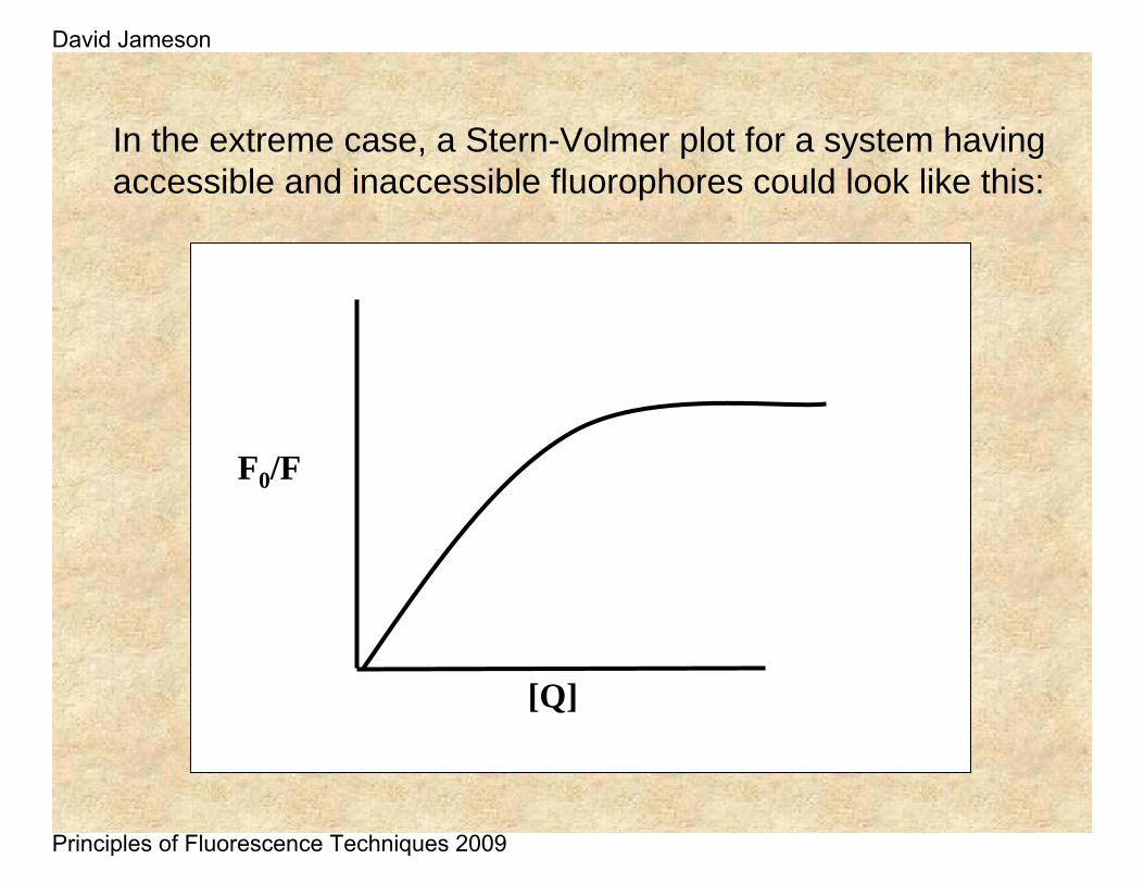
In the extreme case, a Stern-Volmer plot for a system having accessible and inaccessible fluorophores could look like this:

F0/F

[Q]

David Jameson


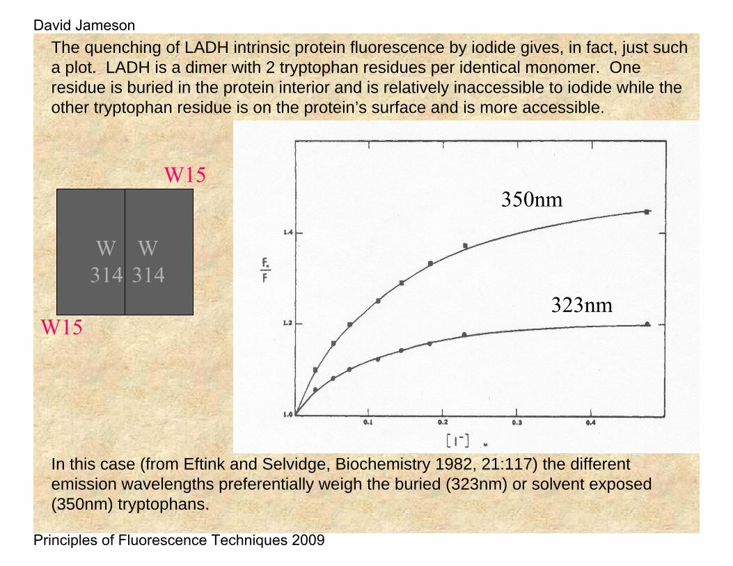
323nm

350nm

In this case (from Eftink and Selvidge, Biochemistry 1982, 21:117) the different emission wavelengths preferentially weigh the buried (323nm) or solvent exposed (350nm) tryptophans.

The quenching of LADH intrinsic protein fluorescence by iodide gives, in fact, just such a plot. LADH is a dimer with 2 tryptophan residues per identical monomer. One residue is buried in the protein interior and is relatively inaccessible to iodide while the other tryptophan residue is on the protein’s surface and is more accessible.

W15

W314

W314

W15

David Jameson


Documents

Principles of Fluorescence Techniques 2009 … Fluorescence Principles II: David Jameson Time-Resolved Fluorescence and Quenching Principles of Fluorescence Techniques 2009 Chicago,