University of North Carolina Wilmington Cameron School of Business

Department of Economics & Finance

Principles of Financial Management FIN 335

Phase 2 LECTURE NOTES AND STUDY GUIDE

5th Edition, October 2012

To Accompany Brigham & Houston Fundamentals of Financial Management, Concise 7th Ed.,

South-Western, 2012

Prepared by Dr. David P. Echevarria

ALL RIGHTS RESERVED

2

Chapter 5: TIME VALUE OF MONEY

I. THE TIME VALUE OF MONEY (TVM)

TVM is the basis for analysis of value and understanding value is an important key to wealth. A dollar received tomorrow is not worth as much as a received dollar today. A dollar invested today will earn interest and be worth more than a dollar received tomorrow.

A. Future Value;

1. What $1 invested today should grow to over time at an interest rate i.

2. Notation: FV = future value, P = principal, i = interest rate.

I = interest (dollar amount), I = P i

3. The single interest [n = 1] period

FV = P + I = P + P(i) = P(1+i)

4. Multiple [n > 1] compound periods at rate i;

FVi,n = P (1+i)n

(1+i)n = Future Value Interest Factor (see FVIF table).

FVI,n = P FVIFi,n

Computing the present value (PV) of future amounts to be received is central to the capital budget-ing process to be covered later in this course. In fact, the value of all investments is the present value of all cash benefits to be received in the future. It is a good idea to equate the notion of present value with "price" or "market value."

B. Present Value;

1. The value today of a dollar to be received tomorrow

2. Solving the Future Value Equation for PV;

PV = FV (1+i) single period discounting.

PV = FV (1+i)n multi-period discounting.

PV = FV (1+i)-n common form.

(1+i)-n = Present Value Interest Factor (see PVIF table).

3. Relationship of FVIFi,n and PVIFi,n;

a. FVIFi,n = 1 PVIFi,n.

b. All FVIFs equal to the reciprocals of the PVIFs.

We learn that the more compounding periods per year, the greater the amount of the accumulated prin-cipal plus [reinvested] interest. The most complex scenario is when we have multiple compound periods per year (i.e., monthly or daily compounding) over a period of several years.

II. THE FINANCIAL CALCULATOR: Texas Instruments BA II PLUS

C. Important Operating Points;

Calculators have Non-Volatile Memories.

Most keys have two functions.

{Second Functions} are activated by first using the [2nd] key.

Contents of memory registers can be checked using the RCL (recall) key.

Several function keys open mini-spreadsheets for data entry;

1. [CF] cash flow; Use to enter initial outlay and subsequent inflows/outflows.

3

2. [2nd] [I/Y] {PY} Set payments per year, compound periods per year.

3. [2nd] [7] {Data} Use to enter x and/or y data for statistics and linear regression.

4. [2nd] [9] {Bond} Use to enter bond pricing information.

5. Several Function keys provide outputs based on pre-programmed functions and related data entry.

6. [NPV] Use [CPT] to compute net present value in capital budgeting problems.

7. [2nd] [PV] {Amort} Use for amortization table; data entered in TVM registers.

8. [2nd] [8] {Stat} Use to perform statistics; means, variances, slope and intercept.

D. Layout of Calculator Display and Function Keys

E. Frequently Used Keys [ xxx ]; Second Function { xxx }

9. 1. [CPT] (Compute; used to execute a compute sequence after data is entered).

10. 2. [ENTER] (used to enter values into mini-spreadsheet data registers). When required, the display will show ENTER to remind you.

11. 3. [2nd] {SET} (used to toggle certain operating features; e.g. to turn the BGN (begin) on or off (when off, END shown in display).

12. 4. [2nd] [FV] {CLR TVM} (used to clear al values in the TVM registers ONLY).

13. [2nd] [CE/C] {CLR Work} Use to clear CF, Data, and Depreciation data registers.

14. [] Use to delete last number(s) entered.

15. [2nd] {Format} Use to set decimal places; Enter number, press [ENTER]. [2nd] {quit}

16. [2nd] [+/-] {Reset} Use to reset all parameters to factory settings.

17. 1-1. [CPT]: compute key.

18. QUIT: to leave sub-routine mode.

19. 2-1. [2nd]:Second function key (appears in display when "toggled").

20. 2-2. [CF]: enter cash flows for NPV computations.

4

21. Row 3 contains the Time Value of Money keys and related second functions.

22. 3-1. [N]: Number of periods (weeks, months, years, etc.)

23. a. xP/YR: mult periods per year time number of years.

24. 3-2. [I/YR]: Annual Interest Rate

25. a. P/YR: number of compound periods per year.

26. 3-3. [PV]: To Enter Present Value, or to "compute" PV.

27. a. AMORT: compute principle, interest, and balance (worksheet mode).

28. 3-4. [PMT]: To Enter Payment, or "compute" Payment.

29. 3-5. [FV]: To Enter Future Value, or to "compute" FV.

30. a. CLR TVM: to clear all TVM memory registers.

31. 7-1. [STO]: store values in memory registers (0 thru 9).

32. 8-1. [RCL]: recall values from memory registers.

33. 9-1. [CE/C]: clear display register or pending operation.

34. a. CLR Work: clear mini-spreadsheet data registers.

35. 9-2. [2nd MEM]: permits visual access to the memory worksheet; enter-only function.

Always press the [2nd] key and the [FV] key to clear the Time Value of Money (TVM) registers. Calculators maintain contents in memory registers until erased. To reset decimal places: [2nd] [ . ]. Enter the number of decimal places you want to display (0 - 8), And the [ENTER] key. Turn-ing the BA II PLUS off (ON/OFF key) does not zero the memory registers.

The Guidebook which comes with the BA II PLUS is very well written and has full sets of ex-amples on how to enter data and solve problems. An additional feature is the “QUICK START” insert. This insert takes you step by step through a calculation. It also shows how to reset the calculator. A caution; when you Reset the calculator using the [2nd +/-] Reset and Enter keys, the calculator is returned to factory default values. MAKE CERTAIN THIS IS WHAT YOU WANT TO DO.

F. Single Interest Event versus Multiple Interest Events;

1. What we typically refer to as "compound interest" is really multiple interest events per year; on the BA II PLUS the C/Y function.

2. Interest may be paid semi-annually, quarterly, monthly, weekly, or daily.

3. When there is more than one interest period per year;

a. We divide the "per annum I/Y" by the number of compounding periods per year; i.e., quarterly = 4. The BAII Plus does this automatically when the C/Y value is set.

b. The number of compounding periods per year fixes the periodic interest rate.

(1) What is the daily rate if the per annum (P.A.) rate is 12%?

(2) 12 % P.A. is 12/360 = .03333 % interest rate per day or 0.0003333, the decimal equivalent.

4. When the interest earning period is less than one year;

5. Suppose we want to compute the periodic interest rate for an investment in a savings ac-count for 30 days if the per annum rate is 12%

a. We multiply the per annum rate by (D/360);

b. D = number of days: 12 % P.A. for 30 days; .12 * (30/360) = .01 (1%) for 30 days

5

III. SINKING FUNDS, RETIREMENT PLANS, AND INSURANCE ANNUI-TIES

In a sinking fund, we assume that we are making periodic deposits into a plan in order to ac-cumulate a certain sum of money at some point in the future. Sinking funds are associated with corporate bond issues. A retirement plan is a systematic savings plan with certain tax ad-vantages. Both plans require regular deposits. These funds are then invested in marketable secu-rities (i.e., stocks and/or bonds). The future value of the accumulation includes principal paid in and reinvested interest, dividends, and/or capital gains. A large proportion of retirement funds is invested in mutual funds. Insurance annuities are used to provide a fixed payment of money for a predetermined period of time. Some financial planners suggest buying these plans in order to assure a regular payment from the retirement plan accumulation.

We make a distinction between receipts (positive values) and deposits (negative values). We define receipts as positive cash flows; i.e., money that we receive. We define deposits as negative cash flows; i.e., money paid into a systematic savings or retirement plan. Later on, we will use the financial calculator to compute various items of interest. It is important to understand that cash flowing away from us is treated as a negative cash flow while cash flowing to us is a posi-tive cash flow. For example; when we make a car payment, it’s a negative cash flow. If we de-posit monies into a savings plan, that’s also a negative cash flow. When we make a withdrawal from our savings plan, it’s a positive cash flow.

A. In this section we determine;

1. The price we must pay (PV) to receive a certain amount of income.

2. How much income (PMT) a certain accumulated (FV) amount will produce.

3. How much we will accumulate given a rate of interest assumption

4. Annuitize the accumulation and determining the amount of the payout.

B. Annuities

1. [Insurance] annuities provide recipient with a known income for a set period of time.

2. The present value of the payments to be received is the price of the insurance annuity.

C. Types of Annuities:

1. Ordinary Annuity: payments received at end-of-period.

2. Annuity Due: payments received at beginning-of-period

Students should make certain that the "BEGIN" flag is off. In the BAII Plus the "BEGIN" flag, if on, will appear in the display as “BGN”. We use the "BEGIN" function when we assume depos-its or receipts occur on the first day of the interest period rather than the last; an Annuity Due. The effect is an extra period of interest to compound or discount. It will make FVA and PVA larger.

D. Regular Savings or Retirement Plan; Future Value of the Accumulation (FVA)

1. An annuity is series of equal deposits (contributions) over some length of time.

2. Contributions are invested in financial securities; stocks, bonds, mutual funds.

3. The future value of accumulation is a function of the number and magnitude of contributions, reinvested interest, dividends, and undistributed capital gains.

4. The future value of an accumulation (FVA) formula;

5. FVA = P ([(1+i)n - 1] i) = P FVIFA

6. Where: P = periodic regular deposit.

7. (1+i)n - 1] i = future value interest factor for an annuity or FVIFAi,n

6

8. An alternate way to compute the FVIFA; summing FVIFs

a. = “Sum of” symbol

b. Assume: steady growth rate over time and equal dollar amount contributions.

IV. SAMPLE PROBLEMS: COMPUTING FUTURE VALUES

A. IRA Accumulations;

Suppose you want to know how much an IRA (individual retirement account) plan will grow to if you deposit $2,000 per year (the maximum under current law) or $166.67 per month every month for the next 20 years. We’ll assume monthly compounded interest and annual rate of 9 percent (9% per annum). What is the Future Value of the Accumulation (FVA)? (First set the calculator to 5 decimal places using the Format function.)

1. First compute the FVIFA for 9% divided by 12 and 20 years times 12 months.

9% per Annum divided by 12 = .75% per month (i); the periodic rate.

20 years 12 months per year = 240 months (n); the number of compound periods.

2. The FVA is found by multiplying the monthly deposit by the FVIFA;

a. FVA = 166.67 667.88687 = $111,316.70

FVIFA = [(1.0075)240 1]

.0075667.886870.0075,240

3. Let’s do this same problem using the BA II PLUS.

Always clear the TVM registers; press [2nd], then [FV] (CLR TVM).

Press [2nd I/Y] for the P/Y function; enter 12, then press [ENTER] and [] for C/Y regis-ter; enter 12, then press [ENTER], then [2nd CPT] to QUIT this subroutine. If these values are already stored, then quit subroutine.

Enter 240, press [N].

Enter 9, press [I/Y]; interest rate per annum.

Enter 166.67, then [+/-] and then [PMT].

Press [CPT] then [FV]; 111,316.70461 appears in the display.

Don't clear the values yet. We're going to use them in the next problem.

B. Effects of Time and Rate of Return on Accumulations;

The BA II PLUS allows us to perform a sort of "what if" simulation. We can re-enter a new val-ue for any variable and compute the desired variable. In this example we are going to compute the FVA given a change in the time period for the accumulation.

1. What effect does an extra 10 years of $166.67 deposited per month have on the FVA? How much will the FVA be after 30 years of monthly savings?

Enter 30, press [2nd N], then press [N] again. We use the calculator to compute how many months are in 30 years (360). You must press the [N] to save this value.

Press [CPT] [FV]; $305,130.01632 is the FVA if we assume an extra 10 years of monthly deposits.

The total deposits are 166.67 * 360 = $60,001.20. The other $245,128.82 is the accumu-

FVIFAi,n

( )1 1

1

i t

t

n

7

lated interest.

2. What effect does the rate of return have on the size of the accumulation? Suppose the in-terest rate was 12%, what is the FVA?

Enter 12, press [I/Y].

Press [CPT] [FV]; $582,505.67201 is the FVA if we assume 30 years of monthly depos-its of 166.67 accumulating at 12% per annum compounded monthly.

C. Other Types of Retirement Savings Plans;

1. 401(k) plans; company and individual contributions.

2. 403(b) plans; used by non-profit organizations.

3. SEP plans; plans fore the self-employed.

4. Keough Plans; for professionals such as doctors and lawyers.

V. SAMPLE PROBLEMS; ANNUITIZING ACCUMULATIONS

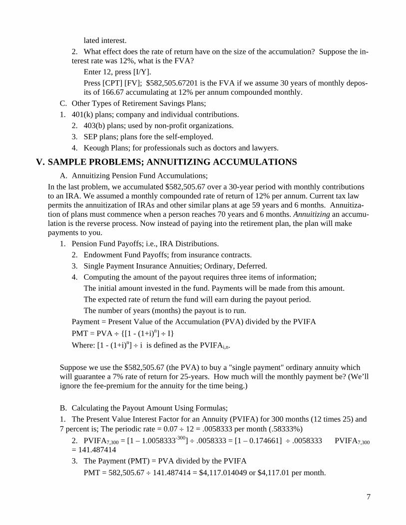
A. Annuitizing Pension Fund Accumulations;

In the last problem, we accumulated $582,505.67 over a 30-year period with monthly contributions to an IRA. We assumed a monthly compounded rate of return of 12% per annum. Current tax law permits the annuitization of IRAs and other similar plans at age 59 years and 6 months. Annuitiza-tion of plans must commence when a person reaches 70 years and 6 months. Annuitizing an accumu-lation is the reverse process. Now instead of paying into the retirement plan, the plan will make payments to you.

1. Pension Fund Payoffs; i.e., IRA Distributions.

2. Endowment Fund Payoffs; from insurance contracts.

3. Single Payment Insurance Annuities; Ordinary, Deferred.

4. Computing the amount of the payout requires three items of information;

The initial amount invested in the fund. Payments will be made from this amount.

The expected rate of return the fund will earn during the payout period.

The number of years (months) the payout is to run.

Payment = Present Value of the Accumulation (PVA) divided by the PVIFA

PMT = PVA {[1 - (1+i)n] I}

Where: [1 - (1+i)n] i is defined as the PVIFAi,n.

Suppose we use the $582,505.67 (the PVA) to buy a "single payment" ordinary annuity which will guarantee a 7% rate of return for 25-years. How much will the monthly payment be? (We’ll ignore the fee-premium for the annuity for the time being.)

B. Calculating the Payout Amount Using Formulas;

1. The Present Value Interest Factor for an Annuity (PVIFA) for 300 months (12 times 25) and 7 percent is; The periodic rate = 0.07 12 = .0058333 per month (.58333%)

2. PVIFA7,300 = [1 – 1.0058333-300] .0058333 = [1 – 0.174661] .0058333 PVIFA7,300 = 141.487414

3. The Payment (PMT) = PVA divided by the PVIFA

PMT = 582,505.67 141.487414 = $4,117.014049 or $4,117.01 per month.

8

C. Calculating the Payout Amount Using Financial calculator;

1. First clear the TVM registers by pressing [2nd FV] (CLR TVM).

2. Enter 300 and press the [N] key.

3. Enter 7 and press the [I/Y] key.

4. Enter 582505.67. Press the [+/-] key, then the [PV].

5. Press the [CPT] key then the [PMT] key;

6. The amount $4,117.028913 appears in the display.

7. The total payout over 25 years = $4,117.03 times 300 = $1,235,109.

An investment of $60,000 produced benefits worth $1.235 million. Obviously this is an example and is predicated on earning a fixed rate during the accumulation and payout phases of this plan. Accumulations and payout benefits will vary depending on your assumed rates and contribution amounts. The moral of this story is quite simple; the accumulation of wealth takes time and self-discipline. The trick is to start early and keep it going.

D. Calculating the Price an Insurance Annuity [Policy] using Formulas;

Suppose we have a fixed payout amount in mind. How much must we pay for an annuity con-tract that will pay a fixed amount for a fixed length of time? Suppose we desire to collect $5,000 per month for 20 years (240 payments) and the rate of return is 9% compounded monthly.

1. Pricing an annuity contract when the payment is known;

a. PVA = P * PVIFAi,n

i = 0.09 / 12 = 0.0075 (i per month), 12 * 20 = 240 (months)

PVIFA 0.0075, 240 = ([1 - (1.0075)-240 / .0075) = 111.14495

PVA = 5,000 * 111.144954 = $ 555,724.77

2. PVA = cost of a "single payment" ordinary annuity to be immediately annuitized.

E. Calculating the Price an Insurance Annuity [Policy] using Financial Calculator;

1. Clear the TVM registers.

2. Enter 240 and press [N].

3. Enter 9 and press [I/Y].

4. Enter 5000 and press [PMT].

5. Press [CPT] and [PV].

6. The display should show; “PV = -555,724.77” or $555,724.77 is price of annuity.

a. The negative sign reminds us that this is a price (negative cash flow).

*** TIME AND THE VALUE OF MONEY! ***

9

VI. AMORTIZATION SCHEDULES; CALCULATING LOAN PAYMENTS

A. Calculating Monthly Car Payments

How much will the monthly payments for a $16,000 automobile loan be if the per annum rate is 9.125% and the term is 5 years (60 months)? We'll solve this problem using the BA II PLUS.

It's always a good idea to start out by clearing the TVM registers and then checking the P/Y and C/Y values; [2nd] [FV] {CLR TVM}, [2nd] [I/Y] {P/Y} and the [] to check the C/Y value. [2nd] [CPT] {QUIT} gets you back to the data input mode.

1. Press [2nd] [FV] {CLR TVM} to clear the registers.

2. Check the values set for P/Y and C/Y. Reset as necessary, then [2nd] [CPT] {QUIT}.

3. Enter 5, press [2nd] [N]; then [N].

4. Enter 9.125, press [I/YR].

5. Enter 16000, press [PV]; you're receiving a $16,000 loan.

6. Press [CPT] [PMT]; -333.11 or $ 333.11 monthly payment.

7. What would the monthly payment be if you finance for 48 months?

B. Calculating Mortgage Payments;

How much will monthly mortgage payments be on a $150,000 mortgage if the term is 30 years and the rate is 10%? Using the BA II PLUS.

1. Clear the memory registers, check the "P/Y" and "C/Y" for values of 12 each.

2. Enter 30, press [2nd N] (xP/Y), then [N]; “N = 360.00” should appear in the display.

3. Enter 10, press [I/YR]; “I/Y = 10.00” should appear in the display.

4. Enter 150000, press [PV]; “PV = 150,000.00” should appear in the display.

5. Press [CPT] [PMT]; “PMT = -1,316.36” should appear in the display indicating a $1,316.36 monthly payment to amortize a mortgage of $150,000 over 30 years.

The $1,316.36 represents the payment of principal and interest due. How much of the first payment is interest and how much is principal? In order to answer this question we will use the AMORT worksheet function of the BA II PLUS.

6. Press [2nd] [PV] {AMORT} to activate the amortization worksheet functions.

7. You should see “P1 = 1.00” in the display. Now press the [] key; you should see P2 = 1.00 in the display. Press the [] key again.

8. Press the [] key; "BAL" = 149,933.64 new remaining loan balance.

9. Press the [] key; "PRN" = -66.36 applied toward the principal.

10. Press the [] key; "INT" = 1,250.00 interest on the old outstanding balance.

VII. AUTOMOTIVE LEASES AND BIWEEKLY MORTGAGES

A. Automobile Leases and the Implied Borrowing Rate.

Consumers have been leasing cars and sport utility vehicles with increasing frequency in recent years. Leasing of personal autos is an alternative to bank financing. Most lease deals are “sold” to consumers on the basis of the “affordable monthly payment.” An important question relates to the implied borrowing rate. In essence, the dealer borrows the money to sell you the car and then you make the payments. Not so obvious in this scheme is the fact that the dealer frequently grosses up

10

the borrowing rate when computing the necessary monthly lease payment. Most newspaper adver-tisements inform you of:

1. The MSRP (manufacturer’s suggested retail price) of the vehicle,

2. The monthly payment, the cash up front required (sometimes referred to as the capital re-duction fee), the number of months for the lease and

3. The end-of-lease (EOL) payment required if you choose to buy the car.

Knowing what you are paying in the way of lease financing is an important step in becoming a knowledgeable consumer.

VIII. Summary

We can use the BA II PLUS for any number of financial calculations. Later we will learn to use the [CF] key to enter cash flows for a capital investment problem.

Funds invested today grow and compound as the interest previously earned earns more inter-est.

Funds to be received in the future must be discounted to compare their value to funds re-ceived today.

There are four TVM cases: the future value of a dollar, the present value of a dollar, the fu-ture value of an annuity, and the present value of an annuity.

An annuity is a series of equal, annual payments. If the payments are received at the end of the time period, the annuity is referred to as an "ordinary annuity." If the payments are received at the beginning of the time period, the annuity is referred to as an "annuity due."

When annual rates are subject to frequent compounding (i.e., quarterly, monthly, or daily) it is sometimes necessary to compute an effective annual interest rate. The frequently encountered APR (annual percentage rate) is a good example of this concept. Loan rates are generally quoted as per annum rates. Since consumer loans are amortized on a monthly basis, the Truth in Lending Act requires lenders to reveal the effective rate actually paid on a loan.

The BA II PLUS will compute this rate for you. Press [2nd] [ 2 ] (I Conv). Enter the value of the annual interest rate, press [ENTER]. Press the [] and enter the number of compound periods per year in the C/Y register. Press the [] key and then the [CPT] key, read the effective rate (or EAR) in the display. The 1.5% per month on most credit cards or 18% per year is actually an EAR of 19.56182% per annum.

We will learn to use other functions of the BA II PLUS in chapters that follow. It is likely to be one of the best investments you'll make as a student.

IX. Homework Assignments

A. Self-Test: ST-1, c, f, i, j

B. Questions: 5-3, 5-4, 5-5

C. Problems: 5-1, 5-2, 5-3, 5-4, 5-5

11

X. PROBLEMS YOU SHOULD BE ABLE TO DO

All of the following problems you should be able to do either; (a) manually, or (b) using a finan-cial calculator. Obviously, it is faster to use a calculator. However, you should be able to compute the answers by manual methods.

A. If you invest $10,000 today in a certificate of deposit paying 5.3% per annum compounded quarterly, how much will your investment grow to in five years? How much interest income will you earn?

B. How much must you save each month in order to accumulate $10,000 in four years? Your investment plan earns 4.5 percent per annum compounded monthly.

C. ow long will it take for $ 2,000 to quadruple (grow to $8,000) if you invest it at 15 percent per annum compounded weekly?

D. How much must a person save each month in order to accumulate the $ 250,000 in 15 years if they can invest at 12 % per annum, compounded monthly (P/Y, C/Y = 12)

E. Each month Fred will invest $200 in stocks recommended by his stockbroker and will hold them in a self-directed IRA plan. After doing some research on the stock market you find out that the stock market has returned an average of 15% per annum for the last 20 years. If Fred earns 15% per annum on his stock investments (compounded monthly), how much should he have in his portfolio at the end of 30 years?

F. Mr. Jonas has $750,000 in a mutual fund IRA, is 60 years old and wants to retire. His idea is to purchase an insurance annuity that will provide him with a steady, guaranteed income should he desire to retire early. You consult an actuarial table and estimate that a person retir-ing at age 60 can expect to live another 25 years. The insurance annuity plan will make monthly payments and will guarantee 5.25% per annum, compounded monthly. How much will those monthly payments?

G. You are interviewing for a job as a bank financial analyst and the interviewer wants to test your ability to analyze a mortgage problem. She gives you the following information. The principal amount of the mortgage is $ 160,000 and will be amortized monthly over a 30-year period. The interest rate is 6.75 percent per annum. How much is the monthly payment?

H. Prepare a partial Amortization table for payments # 1 through 3 below for the loan described in question # 7. Remember that the AMORT function requires the payment start period num-ber (P1) and the finish period number (P2). For the following table, P1 = P2.

Payment Balance Principal Interest

1

2

3

12

Appendix A to Chapter 5 : Time Value of Money Problems1

I. Computed on a Texas Instrument BA II Plus financial calculator

I. Before you start:

The gray 2nd key activates the functions that appear above the calculator buttons.

Example: Above the PV key, AMORT is written in gray letters. To use it, press 2nd and then press AMORT.

J. IMPORTANT: To clear previous work:

Press 2nd and CLR TVM (Time Value of Money).

Another clearing option is to press 2nd and Reset. It will reset the calculator to its original settings.

K. Data Entry

Most of the data entry will be value first, then the function. Example: press 4, then press N, the display will be N = 4.

Some values MUST be recorded in memory with the ENTER key. Be careful to make sure your entry has been acknowledged by the calculator. It will say the function you want = to the value entered. Example: P/Y = 4 or N = 36.

Make sure the C/Y and P/Y values are the same if not otherwise stated in the problem.

Example: C/Y = 4 and P/Y = 4.

Payments are cash outflows and may appear as negative (-) depending on the calculator used.

II. Sample Problem 1: Computing Effective Rates = Annual Percentage Rate.

L. Given: Pay 8% annually, compounded quarterly. What is the effective rate?

Values:

Periods/yr. = 4 compounded/yr. = 4 Nominal Rate = 8

Calculator:

Press 2nd and then P/Y. Press 4 and then ENTER. It will display: P/Y = 4

Press 2nd and then QUIT. The display will go to 0.

Press 2nd and I CONV (you'll find it above the number 2).

The field NOM will appear. Press 8 and then press ENTER. It will display: NOM = 8.

Press the key and EFF will display.

Press the key again and C/Y will display.

Press 4 and then ENTER. It will display: C/Y = 4.

Press key and return to the EFF display.

Press CPT and the calculator will return the effective rate of 8.24.

1These materials were prepared by Mary Dwyer, a SJU-MBA graduate student at the Albright College Campus.

13

III. Sample Problem 2: Future Value for Single Deposit.

M. Given: What is the future value of $1000 invested today at 8% per annum, compounded quarterly over 5 years?

Values: N = 5 I = 8 PV = 1000 C/Y = 4

NOTE: Five years covers 20 quarters so the N value is not 5 but 20 (5*4).

Calculator:

Press 2nd and P/Y.

Press and C/Y displays. Press 4 and ENTER.

Press 2nd and QUIT. The display will go to 0.

Press 5. Press 2nd and then xP/Y (it appears above N). "20" will display. Press N again. Make sure display reads: N = 20. (Calculator multiplying the C/Y value of 4 by 5.)

Press 1000 and then the PV key. The display should appear as: PV = 1000.

Press 8 and then the I/Y key. The display should appear as: I/Y = 8.

Press the CPT key and then press FV.

The calculator will display the answer of $1,485.95

IV. Sample Problem 3: Sinking Funds or Retirement Plans.

A sinking fund is a series of payments leading to an accumulation. Examples are IRA and 401(K) programs. The payments will be negative (-) values; the Future Value will be positive (+), and the Present Value will be zero (0).

N. Problem:

You want to retire in 30 years. You are starting to invest in a growth income fund that prom-ises an ambitious rate of 15%. You can put in $200 per month. How much will you have in 30 years?

Values:

N = 30 NOTE: The payments will be monthly over 30 years: 30*12 = 360. N = 360

C/Y = 12 P/Y = 12 I/Y = 15 PMT = -200 (Remember payments are negative.)

Calculator:

Press 2nd and then press P/Y. Press 12 and then press ENTER.

Press and C/Y displays. Press 12 and then press ENTER

Press 2nd and then press QUIT.

Press 30. Press 2nd and then xP/Y. 360 will appear. Press N.

N = 360 will display.

Press 15 and then press I/Y. I/Y = 15 will display.

Press 200. Press the +/- key to the left of the = button. This will change the sign of the 200 from positive to negative. The display should be -200. Next press PMT. The display will be PMT = -200.

Press CPT and press FV. The answer displayed will be $1,384,655.92.

14

V. Sample Problem 4: Special Case of the Annuity Problem - Amortization

An amortization is a payment to pay down a loan that has been made in the present.

You have an opportunity to take on a 30 year $100,000 mortgage at 7.5% interest. What will your monthly payments be?

Values:

N = 30 C/Y = 12 P/Y = 12 I/Y = 7.5 PV = 100,000

{NOTE: The payments will be monthly over 30 years: 30*12 = 360. N = 360}

Calculator:

Press 2nd then press CLR TVM to clear out data from previous problems.

Press 2nd and then press P/Y. Press 12 and then press ENTER.

Press and C/Y displays. Press 12 and then press ENTER

Press 2nd and then press QUIT.

Press 30. Press 2nd and then xP/Y (it appears over the N button). 360 will appear. Press N (to store value in “N” register}

N = 360 will display.

Press 7.5 and then press I/Y. The display will be I/Y = 7.5.

Press 100,000 and then press PV.

Press CPT and then press PMT. The payment displayed will be -$699.21.

15

CHAPTER 6: INTEREST RATES

I. Cost of Credit

A. Interest rates reflect the cost of borrowing money (or capital)

B. Four Principal Factors Influencing Rates

1. Investment opportunities

2. Time preferences for consumption

3. Riskiness of objectives

4. Inflation

C. Other Factors Influencing Interest rates.

1. Federal Reserve Monetary Policy.

2. Investor expectations about economy.

3. Business Decisions.

II. TERM STRUCTURE OF INTEREST RATES

A. Normal Yield Curve: relation between time or risk (x-axis) and return (y-axis)

1. Upward sloping to the right

2. The higher the risk, the greater the required rate of return

B. Inverted Yield Curve

1. Downward sloping to the right

2. When short-term risk or inflation is greater than longer term levels.

C. Composition of Nominal Interest Rates.

1. Real rate of return.

2. Inflation premium.

3. Default premium.

4. Liquidity premium.

5. Maturity Risk premium

D. r = r* + IP + DRP + LP + MRP

r = required return on a debt security

r* = real risk-free rate of interest

IP = inflation premium

DRP = default risk premium

LP = liquidity premium

MRP = maturity risk premium

III. HOMEWORK ASSIGNMENT

E. Self-Test: ST-1, parts b, c, d, e, f

F. Questions: 6-1, 6-3, 6-8, 6-9

G. Problems: 6-2, 6-5

16

CHAPTER 7: BOND VALUATION

I. CHARACTERISTICS OF ALL DEBT INSTRUMENTS

A. Interest (coupons) and maturity value ($1000 for corporate bonds).

B. Indenture Agreement,

1. Loan contract between lender and company.

2. Appoints the trustee; a fiduciary responsible for guarding the lenders' interests.

3. Terms and conditions, legal remedies.

C. Sources of risk

1. Default = probability of not getting all of the promised interest and principal.

2. Price fluctuations = changes in prices as interest rates change over time.

3. Loss of purchasing power = effects on inflation on coupon income.

II. II. TYPES OF CORPORATE DEBT

Corporations frequently raise funds by issuing [long-term] bonds. Bonds require the borrower to make periodic payments (interest) and to repay the principal at some specified date in the future (the maturity date). Corporations issue various types of bonds. Some are secured by liens on specific property (mortgage bonds and equipment trust certificates), and other bonds are unsecured (deben-tures) which are backed only by the creditworthiness of the firm. Convertible bonds allow the bond investor to exchange the bonds for the company's common stock. Bondholders will do so if it be-comes profitable to convert, otherwise they can continue to enjoy reasonably high interest income.

A. Mortgage bonds: bonds secured by real property

B. Equipment trust certificates: bonds secured by equipment (rolling stock)

C. Debentures: unsecured bonds (no collateral).

D. Income bonds: interest paid only if a specified level of earnings is achieved

E. Convertible bonds: bonds that may be converted into the firm's common stock

F. Variable interest rate bonds: coupons that change with changes in interest rates

G. Zero coupon bonds:

1. Do not pay coupons.

2. Sold for present value of the maturity value ($1000)

H. “Junk” bonds: bonds with low credit ratings

I. Eurobonds: bonds issued abroad denominated on dollars or other currency.

III. III. BOND VALUES AND BOND YIELDS

A. Bond valuation model; Vb = Coupon * PVIFA + Face Value * PVIF

The [I/Y] or [ i ] is the currently required Yield to Maturity (YTM). Face Value [FV] is always $1,000 for a corporate and many municipals. Treasuries tend to have significantly higher Face Values ($250,000). Bond prices fluctuate with changes in interest rates. When interest rates rise, bond prices fall and vice-versa. The current price of a bond depends on how much interest it pays, how long before it matures, and what investors can earn on comparably risky bonds. The bond valuation formula implicitly assumes that all future cash flows (i.e., coupons) are reinvest-ed at the YTM. When this assumption is violated, then the value of bond is different from the theoretical value (the calculated PV).

B. Inverse relationship between a bond's price and interest rates;

17

3. YTM go up --- bond prices go down and vice-versa.

4. If the company gets riskier, then YTMs go up, prices down and vice-versa.

C. Current yield = coupon divided by the price (PV)

The current yield tells the investor the annual percentage rate earned given the bond's current market price. This yield does not consider changes in the bond's price that may occur if the bond is held to maturity. If the bond is held to maturity, the total return is de-fined as the yield to ma-turity, which considers not only the current price but whether the bond is selling for less than face value (i.e., at a discount) or for greater than face value (i.e., at a premium).

D. D. Yield to maturity (YTM);

Investors continually test the risk waters and adjust their bid/ask prices accordingly. If prices are bid up, YTMs are forced down (and vice-versa). Bonds purchased at discount (below par value) accrue a capital gain in addition to the coupon. The capital gain makes the YTM greater than the current yield. If bonds are purchased at a premium (above par value), then the capital loss makes the YTM less than the current yield. Investors buy the YTM on bonds. As bonds approach their maturity date, the current yield and the yield to maturity converge; become nearly equal. At ma-turity, the YTM is identical to the bond's coupon rate.

IV. RETIREMENT OF CORPORATE DEBT

All bonds in an issue mature at the same time. Bonds issued with varying maturities are called serial (redemption) bonds. Corporations do not always retire their long term debt; they roll it over instead. Most companies sell new bond issues and use the proceeds to pay off the maturing issue.

Some bond issues have a sinking fund provision in the indenture agreement which re-quires that the firm set aside a sum of money each year to retire the bonds at maturity.

Corporations may also retire bonds by calling them (if the bonds have a call feature) or repur-chasing the bonds in the secondary market. Bonds will be called only if interest rates have fallen and the firm can refinance the debt at lower interest rates.

Companies desiring to permanently reduce their LTD may wait for interest rates to rise and then repurchase the bonds at a discount; the firm can retire the debt for less than its face value and hence realize a gain on the repurchase. However, when the indenture agreement so specifies, corporations may repay the debt as follows;

A. Serial Redemption Bonds; called by lottery for repayment.

B. Sinking funds; Companies regular deposits into trust fund to accumulate FV

C. Other Possible Strategies;

5. 1. The companies may repurchase debt in the secondary bond market; especially if in-terest rates have risen, reducing market values of their bonds.

6. 2. The companies may issue callable debt; early redemption with additional premium. If interest rates drop, firms reduce interest expense by refunding the existing bonds.

V. GOVERNMENT SECURITIES

Governments issue large numbers of bonds ranging from short-term Treasury bills to long-term bonds. State and local governments also issue bonds. The interest paid on state and local gov-

18

ernment bonds is currently exempt from federal income taxation. The interest paid on treasuries is exempt from local taxation.

A. Federal government bills and bonds

7. 1. Interest is taxable by Federal Government but non taxable by State Governments.

8. 2. Price Quotations different from corporate bonds.

B. Tax-exempt municipal bonds

9. 1. The Pre-Tax Equivalent Yield; compare to taxable yields.

10. 2. Interest not taxable by Federal Government.

VI.

VII. USING FINANCIAL CALCULATORS TO COMPUTE BOND VALUES

The value of a bond is a combination of a present value of an annuity (the present value of the coupons to be received and the present value of the face value of the bond.

For example, suppose we have a bond paying a coupon of $120 per year, paid semi-annually. The bond matures in 20 years and has a face value of $1,000.00. If the current yield rates are 9 percent, how much should this bond sell for?

In this type of problem we will use all five TVM keys; N, I/Y, PV, PMT, FV.

Because the bond pays coupons (interest) twice a year, we set the periods per year (P/Y) to 2. The coupon is paid in two $60 installments. Finally, the bond will have a maturity value of $1000.00. You will receive this amount plus the last coupon at maturity (or $1060).

C. BA II PLUS Solution

11. 1. ENTER 20 [2nd] [N], [N]: Display: N = 40.00

12. 2. ENTER 9 [I/Y]: Display: I/Y = 9.00

13. 3. ENTER 60 [PMT]: Display: PMT = 60.00

14. 4. ENTER 1000 [FV]: Display: FV = 1,000.00

15. 5. PRESS [CPT] [PV]: Display: PV = -1,276.02

D. Playing "what if" with Several Different YTM Values.

For example, suppose the YTM is 11 percent; "I/Y" = 11. Enter 11, press [I/Y], then [CPT] , then [PV]; -1,080.23.

If the YTM is 12%; enter 12, press [I/Y], then [CPT], [PV]; PV = 1,000.00 or $1,000.00.

If the YTM is 15%, the price [PV] is $811.08.

The present value of any bond's cash flows DISCOUNTED at an YTM equal to the coupon rate results in a market value equal to the face value of the bond.

VIII. HOMEWORK

A. Self-Test: ST-1, par value, e, h

B. Questions: 7-3, 7-6, 7-8, 7-9

C. Problems: 7-1, 7-8, 7-11 (part a)

19

20

IX. Questions You Should Be Able To Answer; Learning Objectives

1. What is the purpose of the indenture agreement?

2. What are the principal sources of risk when investing in bonds?

3. What is the difference between a mortgage bond and a debenture bond?

4. Be able to compute bond prices and describe effects of YTM changes on prices.

5. What is the difference between a current yield and a yield-to-maturity?

6. An 18-years until maturity corporate bond pays an 8.50 percent coupon and is priced at 875.50 per bond. The bonds pay a quarterly coupon and have a face value of $ 1,000. What is the yield to maturity (YTM) of the bonds?

7. If the bonds in question 6 are priced to yield 9.95 %, what should be the price?

21

CHAPTER 08: RISK & RETURN

I. Investment Risk

A. Investment risk is related to the probability of earning a low or negative actual return.

B. The greater the chance of lower than expected or negative returns, the riskier the investment.

C. Risk is measured as a probability distribution

1. Mean expected return ( ̅ ) 2. Standard deviation (s)

3. Note: ̅ and s are sample statistics. and are population parameters (unobserved).

II. Average Returns / Risk 1924 - 2004

Average Standard Return Deviation

Small-company stocks 17.5% 33.1% Large-company stocks 12.4 20.3 L-T corporate bonds 6.2 8.6 L-T government bonds 5.8 9.3 U.S. Treasury bills 3.8 3.1

Source: Based on Stocks, Bonds, Bills, and Inflation: (Valuation Edition) 2005 Yearbook (Chicago: Ibbotson Associates, 2005), p28

III. Analysis of Standard Deviations

A. Standard deviation (si) measures total, or stand-alone, risk.

B. The larger si is, the lower the probability that actual returns will be closer to expected returns.

C. Larger si is associated with a wider probability distribution of returns (e.g.; firm Y)

D. Standard deviations are scale sensitive.

IV. Scale-Free Measure of Risk

A. Coefficient of variation (CV): A standardized measure of dispersion about the expected val-ue, that shows the amount of risk per unit of return.

Average Standard Coeff. of Return Deviation Variation

Small-company stocks 17.5% 33.1% 1.89 Large-company stocks 12.4 20.3 1.64 L-T corporate bonds 6.2 8.6 1.39 L-T government bonds 5.8 9.3 1.60 U.S. Treasury bills 3.8 3.1 0.82

22

V. Investor Attitude Towards Risk

A. Investors are assumed to be risk averse.

B. Risk aversion – assumes investors dislike risk and require higher rates of return to encourage them to hold riskier securities.

C. Risk premium – the difference between the return on a risky asset and a riskless asset, which serves as compensation for investors to hold riskier securities.

VI. Managing Investor Risk

A. Primary Strategy to Manage Risk

1. Holding a diversified portfolio of securities

Stocks (common, preferred, foreign)

Bonds (treasury, municipal, corporate)

Mutual Funds (Growth, Income, Balanced, etc.)

B. Sources of Portfolio Risk

1. Firm-specific (diversifiable, non-systematic risk)

2. Market related (non-diversifiable, systematic risk)

C. Correlation

1. Positive (two stocks move in same direction)

2. Negative (two stocks move in opposite direction)

3. Zero (two stocks move randomly)

VII. Capital Asset Pricing Model

A. Asset Pricing Theory seeks to explain why certain assets have higher expected returns than other assets and why expected returns vary over time. Expected returns are those returns when assets are priced in equilibrium:

B. Demand for assets = Supply of assets.

C. CAPM Measures Risk (beta) relative to the Market

D. CAPM suggests that a stock’s required rate of return equals the risk-free return plus a market risk premium multiplied by (measure of relative risk)

E. ri = rRF + (rM – rRF) i

F. Primary conclusion: The relative riskiness of a stock (b) is its contribution to the riskiness (Pf Beta) of a well-diversified portfolio.

VIII. Market Risk Premium

G. M.R.P. = (rM – rRF)

1. Additional return over the risk-free rate needed to compensate investors for assuming an av-erage amount of risk.

H. Price of Risk = (rM – rRF) i

2. Its magnitude depends on the stock’s beta (b), the expected market return and the ex-pected return on the risk-free asset (i.e., 30-day T-Bill)

3. Varies from year to year, but most estimates suggest that it ranges between 4% and 8% per year.

23

IX. The Search for “Alpha”

A. Regression Estimates: y = a + bx + e

1. a is the intercept, is also termed the idiosyncratic return for the random asset y. Investors pre-fer stocks with positive alphas.

2. b, the slope coefficient, becomes the beta of the pricing equation.

3. e, is the random error term.

X. HOMEWORK CHAPTER 8

A. Selt-Test: ST-1, parts a, c, e, i

B. Questions: 8-2, 8-4

C. Problems: 8-1, 8-3, 8-68-1, 8-3, 8-6

24

CHAPTER 9: STOCKS AND THEIR VALUATION

I. PREFERRED STOCK

A. Hybrid Security;

1. PS have fixed [dividend] payouts like bonds

2. PS are equity investments similar to common stock.

3. Preferred stocks are riskier than bonds

4. Dividends paid from after tax income.

B. Attributes of Preferred Stock

1. Par value.

2. Cumulative Features; missed dividends must be made up.

3. Participating; in years of high profits, an extra dividend.

4. Non-Voting; except as provided in corporate charter.

5. Convertibility; typically into common.

6. Some dividends are partially tax exempt (returns of capital).

II. COMMON STOCK

A. Corporate Charter; specifies rights of stockholders

1. Voting to elect directors.

a. Direct or via proxy; power to cast ballot.

b. Majority; if you own 50.1%, you elect all directors.

c. Cumulative; votes * directors, preserving minority interests.

2. Voting to amend the charter.

3. Voting to raise capital.

4. Voting to enter into mergers.

5. Preemptive rights; maintain proportionate ownership share.

B. Classes of Common

1. Voting; the "vanilla flavor."

2. Non-Voting: some classes may be non-voting (unusual).

C. Dividend Policy

1. Declaration date, Record date, and Payment date.

2. Cash vs. Stock Dividends vs. Stock Splits

3. Automatic Dividend Reinvestment Plans

D. Repurchase Of Stock

1. Implied statements about investment opportunity set.

2. An important alternative to paying cash dividends to increase/maintain values

3. Reduction in outstanding shares makes shares more expensive.

25

III. VALUATION OF PREFERRED STOCK

The valuation of preferred stock is essentially the same as the valuation of bonds. The fixed divi-dend payment is subject to the discounted future cash flows method. When interest rates rise the value of preferred stock falls and vice-versa. Hence, preferred stock prices behave very much like bond prices.

E. A. Valuation model; the perpetuity assumption.

psPS r

DIVV

F. B. Impact of changes in interest rates; bond-like behavior.

1. Preferred Stock dividends tend to be fixed.

2. Fixed dividends makes preferred stock prices sensitive to changes in interest rates.

IV. VALUATION OF COMMON STOCK

A. Dividend-Growth Valuation Model

Common stock prices depend on the firm's dividend, the rate of growth in earnings, and inves-tors' required rates of return. In its simplest form, the required rate of return depends on expected dividends and capital gains, and the anticipated level of risk.

1. Zero Growth Model (same as preferred model).

2. Normal Growth; the growth in dividends over time.

B. P/E Ratios & Valuation of Common Stock;

1. Normal valuation models not viable for non-dividend paying stocks.

2. Models don't capture other aspects of firm (non-income items).

3. Implied Earnings-Yield (E/P ratio).

V. HOMEWORK

A. Self-Test: ST-1, a, b, f

B. Questions: 9-2

C. Problems: 9-1, 9-3, 9-6

VD

kee

1

VD

k gee

1

26

VI. QUESTIONS YOU SHOULD BE ABLE TO ANSWER; LEARNING OB-JECTIVES

A. What characteristic of preferred stock causes sensitivity to interest rate changes?

B. What does it mean when a preferred stock is issued cumulative & participating?

C. Why is cumulative voting for directors an important feature of common stock?

D. What are preemptive rights and why are they important to common stockholders?

E. Dividends are subject to double taxation. Why might stockholders prefer the company to re-invest all earnings in the company rather than pay dividends?

F. Why is the record date for dividends important to stockholders and the markets?

G. What reasons are given to explain stock repurchases by the company?

H. What are the important assumptions in the stock valuation model?

I. The stock of Cincinnati Can (CAN) is currently paying a dividend of $ 3.25 and the dividend has been growing at 6 percent per year. The world can market appears to be very risky right now. Accordingly, you believe you require a 13 percent rate of return on the common (Ks). How much should you pay for CAN's stock?

27

CHAPTER 10: COST OF CAPITAL

I. TYPES OF CAPITAL

A. LONG-TERM DEBT (BONDS)

B. PREFERRED STOCK

C. COMMON STOCK (PAID-IN-CAPITAL)

D. RETAINED EARNINGS

II. SOURCES OF LONG-TERM CAPITAL

A. From Most to Least Used Sources

1. Retained Earnings

2. Sale of Corporate Bonds

3. Sale of Common Stock

4. Sale of Preferred Stock

B. Cost of capital determined by firm's capital structure (RHS of B/S).

Capital consists of:

1. Debt (bonds)

2. Equity (preferred and common stocks)

3. Retained Earnings

C. Market-based weighted-average of these costs (WACC) is also termed the hurdle rate.

WACC = Wd Kd (1-t) + Wp Kp + We Ke

D. How are the weights Wi determined?

1. Use accounting numbers (easiest – uses book values)

2. Use market value of issued securities (preferred method)

3. Firm’s cost of capital is set by market forces via investor pricing activity [implied risk as-sessment]

a. High risk: lower prices (low P/E ratios)

b. Low risk: higher prices (high P/E ratios)

III. HURDLE RATE [WACC or ka]

A. Some Observations:

1. Approximately 80% of all investment projects are financed internally (from retained earnings and tax-shielded cash flows such as depreciation).

2. Approximately 15% are financed by selling debt.

3. Approximately 5% are financed by selling stock.

IV. COST OF NEW CAPITAL

A. The Cost of New Debt: Kd

1. Kd = [YTM / (1 - F)] (1 - T)

2. Where:

a. YTM = current market yields to maturity for seasoned bonds. b. F = flotation costs as a decimal (percentage).

28

c. T = the marginal tax rate of the firm B. The cost of Preferred Stock; Kpfd

1. Kpfd = Dpfd / [Ppfd * (1 - F)] 2. Where:

a. Dp = the dividend (to be) paid on the preferred stock. b. Pp = the (current) market price of preferred. c. F = Flotation costs as a percentage

C. Cost of Common Equity (common & retained earns); Ke

Ke = D1 / (Po - F) + g Where:

a. D1 = the expected dividend at the end of year 1. b. Po = the current price of common. c. F = Flotation cost in dollars per share. d. g = the anticipated rate of growth in dividends.

V. HURDLE RATE [WACC or ka]

A. Hurdle rate; minimum rate of return a project must earn. Ceteris paribus….

1. If just the hurdle rate is earned, then value of firm is maintained.

2. If less that the hurdle rate is earned, then value of firm declines.

3. If more that the hurdle rate is earned, then value of firm increases.

VI. HOMEWORK CHAPTER 10

A. Homework Assignment

B. Self-test: ST-1, parts b, e, f

C. Questions: 10-1, parts a, b, h, i

D. Problems: 10-1, 10-3, 10-11

VII. Questions You Should Be Able To Answer

A. Why is the hurdle rate an important concept in capital budgeting?

B. What important considerations must we make when computing the cost of capital?

C. What factors should managers consider when planning a capital structure strategy?

29

CHAPTER 11: BASICS OF CAPITAL BUDGETING

I. INTRODUCTION TO CAPITAL BUDGETING

A. Reasons for Investment Projects

1. Increase sales or diversify product lines.

2. Replace worn-out equipment.

3. Achieve a variety of corporate objectives.

B. How Projects Are Evaluated;

1. Companies have a variety of opportunities.

2. Data is collected on each attractive opportunity.

3. Companies select best investments to increase the value of the firm.

4. They will select as many investments as they have funds.

5. They will seek to diversify their investments in order to diversify their risks.

6. They will periodically reevaluate decisions in order to make decisions relative to continu-ance (abandonment analysis).

C. Learning Objectives

1. To learn the basic methodology for capital budgeting and the relevant decision rules.

2. Minimize the probability of losses; keep in mind that many new products / ventures fail and failures are expensive.

D. Business Objectives

1. Minimize the probability of losses

2. Keep in mind that many new products / ventures fail and failures are expensive.

3. We want to make the most informed decision

E. The Data Inputs; What Information Is Necessary?

1. Type of project; new investment or replacement?

2. Expected economic life of the project (in years).

3. Initial outlay of cash required to finance project.

4. Identifying the timing and magnitude of future cash flows

F. The Hurdle Rate:

In the "time value of money" we are concerned with the present value of an amount to be re-ceived in the future. Capital investments are subject to the same general analysis. We make in-vestments in order to realize future benefits. We are, however, subject to an important con-straint. No one would borrow money at 12% per annum in order to invest it in a business which would earn 9% per annum. Obviously, if we pay 12 and earn 9, we are losing money. Better to stay in bed. The preferred situation is to borrow at 9 and earn 12.

When capital investments are made, an important decision criterion is discount rate (or hur-dle rate) used to compute present values of future benefit streams. The net present value (NPV) of a project is equal to the present value of future cash streams minus the cost of the investment required to produce those cash streams. We will decide to make investments when the NPV is positive.

The hurdle rate is frequently set equal to the cost of capital for the firm. The firm's capital structure consists of debt (bonds) and equity (stocks, and retained earnings). Each of these has a

30

cost. The weighted average of these costs is the most commonly used hurdle rate. The cost of capital for a firm is set by market forces. If a firm is perceived as risky, its cost of capital will be higher, and vice-versa. Investors determine the riskiness of each firm through the prices they are willing to pay for the firm's securities. Low prices reflect high perceived risk, high prices reflect low risk. It is at best an imprecise science.

1. Too high a rate results in many projects being rejected.

2. Too low a rate results in many projects being accepted.

3. We want to earn a rate of return greater than the cost of capital.

4. Firms may use the cost of new capital or the historical cost of capital.

The preferred is the [implied] cost of new capital.

G. Historical vs. Current Market Costs; the important difference

1. Weights should be based on current market costs of capital structure components.

2. Weights should be adjusted if new capital is required and it changes the structure.

3. The capital structure of ABC Corp. is as follows;

LTD: Consists of 10% Coupon Bonds (20 yr.) 15,000,000

Common Equity: Averages 16% Ke 1MM shares 25,000,000

$ 40,000,000

Wd = 15/40 = .375, We = 25/40 = .625, Tax Rate = 34%

WACC = (.375 * .10 * .66) + (.625 * .16) = .02475 + .09375 = .1185 or 11.85%

The current market YTM for debt of companies in the same risk category is 8% and the cost of equity capital, based on current stock prices, is 14%. The 14% cost of equity is based on the following analysis; the stock price is $ 21.875 and is paying a dividend of $1.75. The dividend has been growing at the rate of 6 percent per year for the past several years and is expected to continue at that rate for the foreseeable future. Therefore, Ke = 8% dividend yield plus 6 % growth in earnings and dividends = 14%. The current market value of debt is (ABC pays semi-annual dividends) $17,968,950. ( = 1197.93 per bond at YTM = 8% and 20 years to maturity). The market value of equity is 21,875,000. The market value weights are and

Wd = 17,968,950 / 39,843,950 = .45 We = 21,875,000 / 39,843,950 = .55

WMCC = (.45 * .08 * .66) + (.55 * .14) = .02376 + .077 = .10076 = 10.076 %

The suppliers of capital require, through their pricing activities in the marketplace, a [col-lective] return of 10.076 % on capital invested in ABC. The value would be grossed up by 1 - the percentage flotation cost of any new capital raised by selling additional debt as well as recal-culating the weights and a new adjusted WMCC.

H. Non-Financial Analysis Criterion; what if we don't make the investment?

1. Loss of intangible benefits.

2. Loss of tangible benefits.

31

II. Capital Investment Decision Rules

A. Payback Period

1. How long will it take to recover the initial outlay from ATCF?

2. Ignores the time value of money.

3. Many smaller companies are asked for this information by banks before making loans

B. Net Present Value: NPV >> 0

NPVATCF

kIt

at o

t

n

( )11

Projects with positive net present values add to the value of the firm. Hence we look for projects that have an NPV greater than zero. I prefer the use of the double greater than symbol (>>); meaning much greater than zero. Recall that an important objective of [financial] management is to maximize the value of the firm.

Not so obvious, projects with negative NPV reduce the value of the firm. When the firm loses money, they charge loses against retained earnings (reducing the equity capital of the firm and the value of the firm).

C. Internal Rate of Return: IRR > ka

1. IRR is the discount rate which makes NPV = zero.

2. The assumed reinvestment rate for cash flows.

3. If NPV greater than zero, then IRR is greater than ka.

D. NPV Profile

1. To create a profile, calculate net present value at different discount rates.

2. The rate for a zero NPV is the IRR for the project.

3. See Figure 11.6 on page 386.

E. Problem of Multiple IRR

When cash outflows in subsequent years are great enough to change the net cash flow, we will have an additional solution to the IRR problem. For each change of sign you have another IRR solution.

In these instances, it will be more difficult to make a selection. The NPV method, however, yields a unique solution regardless of the form of the cash flows. When projects have [net] out-flows after the first year, the IRR solution will have more than one root for every instance that net cash flows change sign. The multiple IRR are the result of Descartes' Rule of Signs. Every time a cash flow changes sign, there will be a new (positive, real) root (for the polynomial equa-tion) to the problem. See Figure 11-4.

1. Examples;

a. normally your cash flow looks like the following:

- + + + + 1 change, one solution.

b. some projects may have multiple outflows;

- + + + - + + + 2 changes, two solutions

32

2. Multiple Outflows and Internal Rates of Return

a. the IRR curve will cross the x-axis more than once.

b. multiple cash outflows, one NPV; the one that occurs at the cost of capital.

F. Modified Internal Rate of Return

The NPV and IRR models assume cash flows are reinvested at the WACC or IRR, respectively. Since the IRR may be unattainable over the long run, the MIRR assumes ATCF are reinvested at the WACC. The terminal value (TV) of the reinvested cash flows is discounted at a rate (MIRR) which makes the TV equal to the initial outlay.

III. FIVE STEP CAPITAL BUDGETING PROCESS

A. Proposal Generation: Schedule the Investment Opportunity Set.

Proposals for capital expenditures are made by people at all levels within a business organi-zation. In order to stimulate a flow of ideas that could result in potential cost savings, many firms offer cash rewards to employees whose proposals are ultimately adopted. Capital expenditure proposals typically travel from the originator to a reviewer at a higher level in the organization. Clearly, proposals requiring large outlays will be much more carefully scrutinized than less cost-ly ones.

B. Analysis: Evaluation of Each Opportunity.

Capital expenditure proposals are formally reviewed (1) to assess their appropriateness in light of the firm's overall objectives and plans and (2) more important, to evaluate their economic validity. The proposed costs and benefits are evaluated and then converted into a series of rele-vant cash flows to which a capital budgeting technique is applied in order to measure the invest-ment merit of the potential outlay. In addition, various aspects of the risk associated with the proposal are either incorporated into the economic analysis or rated and recorded along with the economic measures. once the economic analysis is completed, a summary report, often with a recommendation, is submitted to the decision makers).

C. Decision Making: Select the best of the Opportunity Set.

The actual dollar outlay and the importance of a capital expenditure determine the organiza-tional level at which the expenditure decision is made. Firms typically delegate capital-expenditure authority on the basis of certain dollar limits. Generally, the board of directors re-serves the right to make final decisions on capital expenditures requiring outlays beyond a cer-tain amount, while the authority for making smaller expenditures is given to other organizational Levels. Inexpensive capital expenditures such as the purchase of a hammer for $15 are treated as operating outlays not requiring formal analysis. A generally, firms operating under critical time constraints with respect to production often find it necessary to provide exceptional a strict dol-lar-outlay scheme. In such cases the plant manager is often given the power to make decisions necessary to keep the production line moving, even though the outlays entailed are larger than he or she would normally be allowed to authorize.

D. Implementation: Assure Project Development Compliance.

Once a proposal has been approved and funding has been made available, the implementation phase begins. For minor outlays, implementation is relatively routine; the expenditure is made and payment is rendered. For major expenditures, greater control is required to ensure that what has been proposed and approved is acquired at the budgeted costs. Often the expenditures for a single proposal may occur in phases, with each outlay requiring the signed approval of company officers.

33

E. Control: Performance Assessment.

PA involves monitoring the results during the operating phase of a project. The comparisons of actual outcomes in terms Of costs and benefits with those expected and those of previous pro-jects are vital. When actual outcomes deviate from projected outcomes, action may be required to cut costs' improve benefits' or possibly terminate the project.

IV. HOMEWORK

A. Self-test: ST-1, parts b, c, e, g

B. Questions: 11-4, 11-7, 11-9

C. Problems: 11-1, 11-2, 11-4, 11-13

D. Re 11-13: How do the magnitudes of future cash flows influence the IRR? MIRR?

34

Chapter 12: CASH FLOW ESTIMATION AND RISK ANALYSIS

I. Conceptual Considerations

A. Free Cash Flow = EBIT*(1-Tax Rate) – (CapEx + Changes in WC)

B. Accounting Income = Revenues – Expenses*

C. Operating and Non-Operating

D. Incremental Cash Flows: change in total cash flows as the result of an investment decision

E. Sunk Costs: costs incurred in the past which cannot be recovered in the future regardless of the investment decision

II. THE ANALYTICAL METHODOLOGY

A. Tax Considerations When Replacing Old Plant and Equipment.

1. Replacement projects are undertaken to reduce costs.

2. The project may involve the sale of the old asset.

Under the tax reform act of 1986, business assets are depreciated to a zero salvage value for tax purposes. There may or may not be salvage value. Whenever there is salvage value, we must recognize the tax impact. Any proceeds from the sale of the asset above the book value (original cost minus accumulated depreciation) are subject to a tax on the excess above book value. Any losses incurred in disposing of old assets may be written off against taxable income (book value - sale price = loss).

3. Three possible situations when disposing (selling) old assets ;

a. If salvage value < book, then tax credit. The tax credit is a positive cash flow.

b. If salvage value = book, then it's a wash.

c. If salvage value > book, then tax liability. The liability is a negative cash flow.

How much of a credit or liability on your tax bill is determined by the marginal tax rate times the difference between book and selling price.

B. Determining the Initial Investment (Io)

1. The initial investment (or outlay) is the amount of new cash we must provide to launch the venture.

This includes the cost of the new [whatever] plus any tax bill (if we sold the old asset for more than book value, or minus any tax credit (if sold for less than book). It may also include additional working capital needs. i.e., funds for parts, maintenance crews, staff, etc.

2. The initial outlay (Io) is assumed to occur on day zero.

C. Nature of Future Cash Flows

1. New projects may support additional sales.

2. New projects may also result in lower costs.

3. All projects must produce additional net cash flows.

4. After-tax cash flows constitute the return on our initial capital investment (Io).

5. For learning purposes, we will generally provide the change in operating income before depreciation and taxes.

6. Depreciation expense is an important tax shield consideration.

35

Depreciation schedules are determined by the asset’s MACRS class. Once we determine the expected economic life of the project, we use the appropriate MACRS schedule.

See Table 12A.2 for MACRS depreciation schedules (3-, 5-, 7- and 10-year life)

7. The following table is utilized for capital budgeting;

OPERATING CASH FLOW TABLE

YEAR 1 2 3 N

EBDT

DEPR

EBT

TAX

EAT

DEPR

OCF

8. The Net Present Value of a Project (NPV);

a. Sum of the present value of future operating cash flows (OCF) minus the initial out-lay;

b. Discount rate is given as the weighted average cost of capital (ka).

NPV = (OCFn / (1+ka)n) - Io

III. ANCILLARY CONSIDERATIONS IN CAPITAL BUDGETING

A. Types of Projects

1. Mutually Exclusive Projects: competing projects which accomplish the same objective-task. Only 1 is chosen.

2. Independent Projects: projects which accomplish different objective-tasks. More than one selected. How many is determined by capital availability.

B. Fisher's Separation Theorem (1930);

An extension of the Fisher Separation theorem suggests that we separate the investment deci-sion from the financing decision.

The implication is that investment projects should be considered independently of the financ-ing decision. This is a convenient fiction.

Not so obvious, we must consider where our capital is coming from and the impact it will have on the capital structure of the firm.

IV. Risk Analysis

A. The riskiness of a potential investment can best be approximated by sensitivity analysis

1. Changes in the cost of equipment or construction

2. Changes on Production Costs: Fixed, Variable

3. Changes in Expected Sales

36

4. Changes in the Cost of Capital

5. Changes in Tax Rates

B. Sensitivity can best be gauged using an NPV profile

1. A steep curve is implies more sensitivity to small changes inATCFs

2. A shallow curve suggest less sensitivity to small changes in ATCFs

V. CAPITAL BUDGETING MODEL

A. The “Macro” Model; includes details of changes in cost structure (VC and FC)

Chg in Sales Revenue (S)

Chg in Variable Costs (Direct Labor, Materials) (VC)

Chg in Fixed Costs (Sell, General, Admin. Expenses) (FC)

Chg in Depreciation (Plus New, Minus Old) (DEPR)

Chg in Earnings Before Taxes (EBT)

Chg in Taxes T * (EBT)

Chg in Net Income (Acct. Income) EBT – T * (EBT)

Plus Chg in Depreciation (DEPR)

Chg in [Net] Operating Cash Flow ATCF = (1 - T) EBT + DEPR

We can modify the equation in order to capture the [interest] tax shield effects of debt financ-ing. (T) rD equals the tax shield benefit of interest expense. The after-tax cost of debt is equal to (1 - T) rD.

OCF = (1 - T) EBIT - (1 - T) rD + DEPR

OCF = (1 - T) EBT + DEPR

While the equation immediately above is exactly the same as that on the prior page, it is in fact different when real numbers are substituted. Herein we demonstrate that the financing deci-sion cannot be separated from the investment decision without impacting the net result.

VI. HOMEWORK

A. Self-Test: ST-1, parts d, e, standalone risk

B. Questions: 12-4, 12-6, 12-9

C. Problems: 12-1, 12-5, 12-9

D. Excel Simulation #2

3. The Excel simulation primarily focuses on sensitivity analysis.

4. Care should be taken when input the various options. Make certain you reset to base val-ues before proceeding to the next option.

37

VII. QUESTIONS YOU SHOULD BE ABLE TO ANSWER; LEARNING OB-JECTIVES

A. How does a new project differ from a replacement project for tax consideration?

B. What are two important strategies for increasing profits?

C. What are the two decision rules used in TVM-sensitive capital budgeting?

D. How does the Payback Period Decision criterion work?

E. Why is the Reinvestment Rate assumption important with regard to NPV? IRR?

F. What happens to the NPV when the Reinvestment Rate Assumption is violated?

G. How do mutual exclusive projects differ from independent projects?

38

CAPITAL BUDGETING CLASS EXERCISE

I. BACKGROUND INFORMATION: NEW PROJECT ANALYSIS

A. New machine cost = $ 240,000

B. Benefit: reduce EBDT by $ 85,000 per year

C. Economic Expected Project Life = 5 years

D. Machine in 3 year MACRS category (ADC % rates = 33, 45, 15, 7 for years 1,2,3,4)

E. Expected Salvage Value at end of 5th year = $ 20,000

F. Startup Working Capital required = $ 24,000 (to be recouped at end of 5th year)

G. Tax rate = 35%, WACC = 10%

COMPUTING DEPRECIATION SCHEDULE Table 1

DEPRECIATION SCHEDULE FOR NEW MACHINE

YEAR ACRS% COST ADC ACDEP BV

1 0.33

2 0.45

3 0.15

4 0.07

COMPUTE THE AFTER TAX BENEFITS OF COST SAVINGS NOTE: There is no depreciation charge in year 5 for the new machine.

Table 2 YEAR 1 2 3 4 5

EBDT 85000 85000 85000 85000 85000

DEPR

EBT

TAX

EAT

DEPR

ATCF

WC recoup

Sale

Tax @35%

Net ATCF

NPV = _____________ IRR = _____________ MIRR = ________________