Embed Size (px)
DESCRIPTION
Chapter 2 Road Vehicle Performance
Citation preview
Solutions Manual to accompany
Principles of Highway Engineering and Traffic Analysis, 4e
By Fred L. Mannering, Scott S. Washburn, and Walter P. Kilareski
Chapter 2 Road Vehicle Performance
U.S. Customary Units
Copyright © 2008, by John Wiley & Sons, Inc. All rights reserved.
Solutions Manual to accompany Principles of Highway Engineering and Traffic Analysis, 4e, by Fred L. Mannering, Scott S. Washburn, and Walter P. Kilareski. Copyright © 2008, by John Wiley & Sons, Inc. All rights reserved.
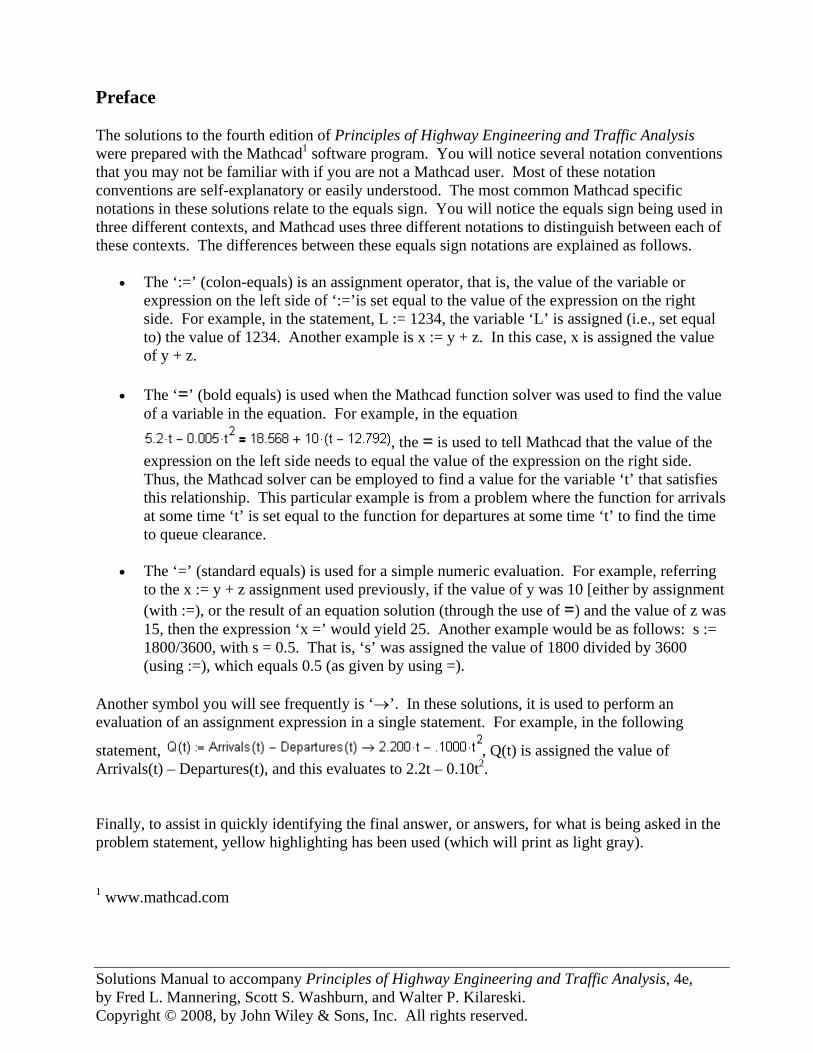
Preface The solutions to the fourth edition of Principles of Highway Engineering and Traffic Analysis were prepared with the Mathcad1 software program. You will notice several notation conventions that you may not be familiar with if you are not a Mathcad user. Most of these notation conventions are self-explanatory or easily understood. The most common Mathcad specific notations in these solutions relate to the equals sign. You will notice the equals sign being used in three different contexts, and Mathcad uses three different notations to distinguish between each of these contexts. The differences between these equals sign notations are explained as follows.
• The ‘:=’ (colon-equals) is an assignment operator, that is, the value of the variable or expression on the left side of ‘:=’is set equal to the value of the expression on the right side. For example, in the statement, L := 1234, the variable ‘L’ is assigned (i.e., set equal to) the value of 1234. Another example is x := y + z. In this case, x is assigned the value of y + z.
• The ‘==’ (bold equals) is used when the Mathcad function solver was used to find the value of a variable in the equation. For example, in the equation
, the == is used to tell Mathcad that the value of the expression on the left side needs to equal the value of the expression on the right side. Thus, the Mathcad solver can be employed to find a value for the variable ‘t’ that satisfies this relationship. This particular example is from a problem where the function for arrivals at some time ‘t’ is set equal to the function for departures at some time ‘t’ to find the time to queue clearance.
• The ‘=’ (standard equals) is used for a simple numeric evaluation. For example, referring to the x := y + z assignment used previously, if the value of y was 10 [either by assignment (with :=), or the result of an equation solution (through the use of ==) and the value of z was 15, then the expression ‘x =’ would yield 25. Another example would be as follows: s := 1800/3600, with s = 0.5. That is, ‘s’ was assigned the value of 1800 divided by 3600 (using :=), which equals 0.5 (as given by using =).
Another symbol you will see frequently is ‘→’. In these solutions, it is used to perform an evaluation of an assignment expression in a single statement. For example, in the following
statement, , Q(t) is assigned the value of Arrivals(t) – Departures(t), and this evaluates to 2.2t – 0.10t2. Finally, to assist in quickly identifying the final answer, or answers, for what is being asked in the problem statement, yellow highlighting has been used (which will print as light gray). 1 www.mathcad.com
Solutions Manual to accompany Principles of Highway Engineering and Traffic Analysis, 4e, by Fred L. Mannering, Scott S. Washburn, and Walter P. Kilareski. Copyright © 2008, by John Wiley & Sons, Inc. All rights reserved.
Solutions Manual to accompany Principles of Highway Engineering and Traffic Analysis, 4e, by Fred L. Mannering, Scott S. Washburn, and Walter P. Kilareski. Copyright © 2008, by John Wiley & Sons, Inc. All rights reserved.
Solutions Manual to accompany Principles of Highway Engineering and Traffic Analysis, 4e, by Fred L. Mannering, Scott S. Washburn, and Walter P. Kilareski. Copyright © 2008, by John Wiley & Sons, Inc. All rights reserved.
Solutions Manual to accompany Principles of Highway Engineering and Traffic Analysis, 4e, by Fred L. Mannering, Scott S. Washburn, and Walter P. Kilareski. Copyright © 2008, by John Wiley & Sons, Inc. All rights reserved.
Solutions Manual to accompany Principles of Highway Engineering and Traffic Analysis, 4e, by Fred L. Mannering, Scott S. Washburn, and Walter P. Kilareski. Copyright © 2008, by John Wiley & Sons, Inc. All rights reserved.
Solutions Manual to accompany Principles of Highway Engineering and Traffic Analysis, 4e, by Fred L. Mannering, Scott S. Washburn, and Walter P. Kilareski. Copyright © 2008, by John Wiley & Sons, Inc. All rights reserved.
Solutions Manual to accompany Principles of Highway Engineering and Traffic Analysis, 4e, by Fred L. Mannering, Scott S. Washburn, and Walter P. Kilareski. Copyright © 2008, by John Wiley & Sons, Inc. All rights reserved.
Solutions Manual to accompany Principles of Highway Engineering and Traffic Analysis, 4e, by Fred L. Mannering, Scott S. Washburn, and Walter P. Kilareski. Copyright © 2008, by John Wiley & Sons, Inc. All rights reserved.

Solutions Manual to accompany Principles of Highway Engineering and Traffic Analysis, 4e, by Fred L. Mannering, Scott S. Washburn, and Walter P. Kilareski. Copyright © 2008, by John Wiley & Sons, Inc. All rights reserved.
Solutions Manual to accompany Principles of Highway Engineering and Traffic Analysis, 4e, by Fred L. Mannering, Scott S. Washburn, and Walter P. Kilareski. Copyright © 2008, by John Wiley & Sons, Inc. All rights reserved.
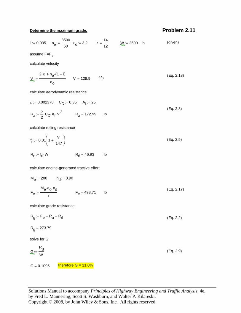
Determine the maximum grade. Problem 2.11
i 0.035:= ne350060
:= εo 3.2:= r1412
:= W 2500:= lb (given)
assume F=Fe
calculate velocity
(Eq. 2.18) V
2 π⋅ r⋅ ne⋅ 1 i−( )⋅
εo:= V 128.9= ft/s
calculate aerodynamic resistance
ρ 0.002378:= CD 0.35:= Af 25:=
(Eq. 2.3)Ra
ρ
2CD⋅ Af⋅ V 2
⋅:= Ra 172.99= lb
calculate rolling resistance
frl 0.01 1V
147+
⎛⎜⎝
⎞⎟⎠
:= (Eq. 2.5)
Rrl frl W⋅:= Rrl 46.93= lb
calculate engine-generated tractive effort
Me 200:= nd 0.90:=
(Eq. 2.17)Fe
Me εo⋅ nd⋅
r:= Fe 493.71= lb
calculate grade resistance
Rg Fe Ra− Rrl−:= (Eq. 2.2)
Rg 273.79=
solve for G
GRgW
:= (Eq. 2.9)
G 0.1095= therefore G = 11.0%
Solutions Manual to accompany Principles of Highway Engineering and Traffic Analysis, 4e, by Fred L. Mannering, Scott S. Washburn, and Walter P. Kilareski. Copyright © 2008, by John Wiley & Sons, Inc. All rights reserved.
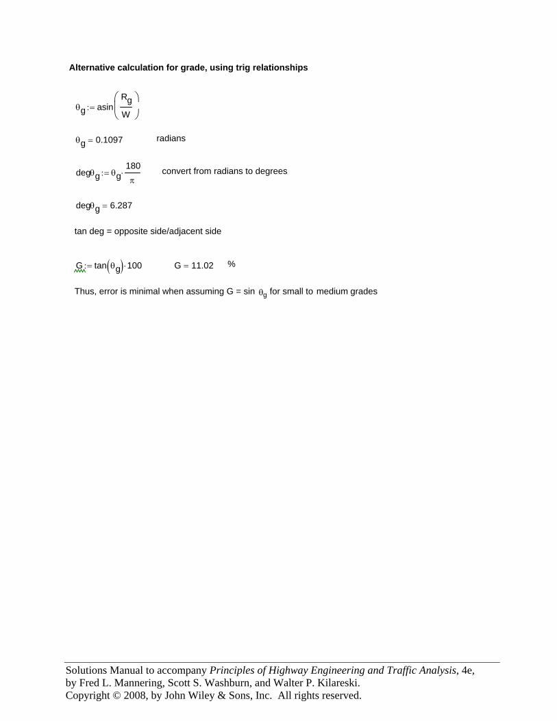
Alternative calculation for grade, using trig relationships
θg asinRgW
⎛⎜⎝
⎞⎟⎠
:=
θg 0.1097= radians
degθg θg180π
⋅:= convert from radians to degrees
degθg 6.287=
tan deg = opposite side/adjacent side
G tan θg( ) 100⋅:= G 11.02= %
Thus, error is minimal when assuming G = sin θg for small to medium grades
Solutions Manual to accompany Principles of Highway Engineering and Traffic Analysis, 4e, by Fred L. Mannering, Scott S. Washburn, and Walter P. Kilareski. Copyright © 2008, by John Wiley & Sons, Inc. All rights reserved.
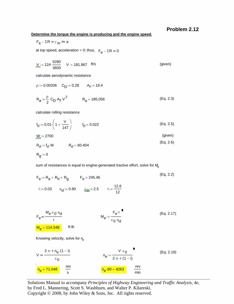
Problem 2.12 Determine the torque the engine is producing and the engine speed.
Fe ΣR− γm m⋅ a⋅
at top speed, acceleration = 0; thus, Fe ΣR− 0
V 12452803600⋅:= V 181.867= ft/s (given)
calculate aerodynamic resistance
ρ 0.00206:= CD 0.28:= Af 19.4:=
Raρ
2CD⋅ Af⋅ V 2⋅:= Ra 185.056= (Eq. 2.3)
calculate rolling resistance
frl 0.01 1V
147+
⎛⎜⎝
⎞⎟⎠
⋅:= frl 0.022= (Eq. 2.5)
W 2700:= (given)
(Eq. 2.6)Rrl frl W⋅:= Rrl 60.404=
Rg 0:=
sum of resistances is equal to engine-generated tractive effort, solve for Me
(Eq. 2.2)Fe Ra Rrl+ Rg+:= Fe 245.46=
i 0.03:= ηd 0.90:= ε0 2.5:= r12.612
:=
(Eq. 2.17)Fe
Me ε0⋅ ηd⋅
rMe
Fe r⋅
ε0 ηd⋅:=
Me 114.548= ft-lb
Knowing velocity, solve for ne
(Eq. 2.18)V
2 π⋅ r⋅ ne⋅ 1 i−( )⋅
ε0ne
V ε0⋅
2 π⋅ r⋅ 1 i−( )⋅:=
ne 71.048=
revs
ne 60⋅ 4263=revmin
Solutions Manual to accompany Principles of Highway Engineering and Traffic Analysis, 4e, by Fred L. Mannering, Scott S. Washburn, and Walter P. Kilareski. Copyright © 2008, by John Wiley & Sons, Inc. All rights reserved.
Solutions Manual to accompany Principles of Highway Engineering and Traffic Analysis, 4e, by Fred L. Mannering, Scott S. Washburn, and Walter P. Kilareski. Copyright © 2008, by John Wiley & Sons, Inc. All rights reserved.
Solutions Manual to accompany Principles of Highway Engineering and Traffic Analysis, 4e, by Fred L. Mannering, Scott S. Washburn, and Walter P. Kilareski. Copyright © 2008, by John Wiley & Sons, Inc. All rights reserved.
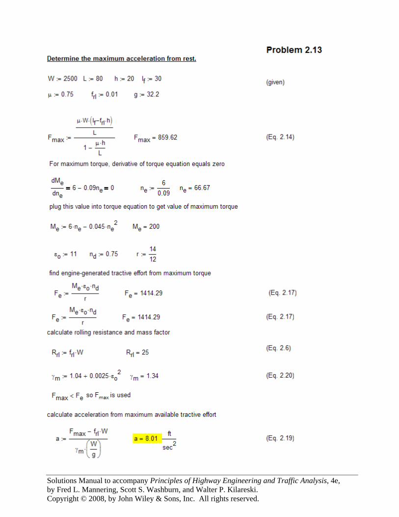
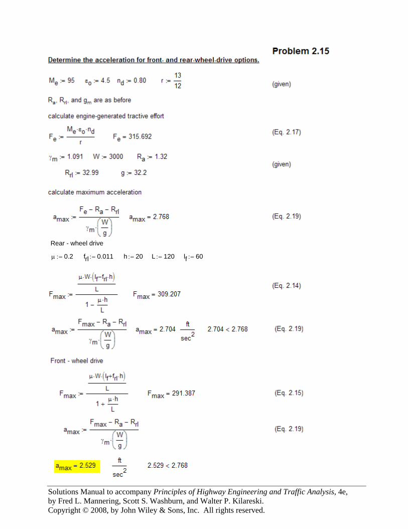
Rear - wheel drive
μ 0.2:= frl 0.011:= h 20:= L 120:= lf 60:=
Solutions Manual to accompany Principles of Highway Engineering and Traffic Analysis, 4e, by Fred L. Mannering, Scott S. Washburn, and Walter P. Kilareski. Copyright © 2008, by John Wiley & Sons, Inc. All rights reserved.
Solutions Manual to accompany Principles of Highway Engineering and Traffic Analysis, 4e, by Fred L. Mannering, Scott S. Washburn, and Walter P. Kilareski. Copyright © 2008, by John Wiley & Sons, Inc. All rights reserved.
Solutions Manual to accompany Principles of Highway Engineering and Traffic Analysis, 4e, by Fred L. Mannering, Scott S. Washburn, and Walter P. Kilareski. Copyright © 2008, by John Wiley & Sons, Inc. All rights reserved.
Solutions Manual to accompany Principles of Highway Engineering and Traffic Analysis, 4e, by Fred L. Mannering, Scott S. Washburn, and Walter P. Kilareski. Copyright © 2008, by John Wiley & Sons, Inc. All rights reserved.
Solutions Manual to accompany Principles of Highway Engineering and Traffic Analysis, 4e, by Fred L. Mannering, Scott S. Washburn, and Walter P. Kilareski. Copyright © 2008, by John Wiley & Sons, Inc. All rights reserved.
Solutions Manual to accompany Principles of Highway Engineering and Traffic Analysis, 4e, by Fred L. Mannering, Scott S. Washburn, and Walter P. Kilareski. Copyright © 2008, by John Wiley & Sons, Inc. All rights reserved.
Solutions Manual to accompany Principles of Highway Engineering and Traffic Analysis, 4e, by Fred L. Mannering, Scott S. Washburn, and Walter P. Kilareski. Copyright © 2008, by John Wiley & Sons, Inc. All rights reserved.
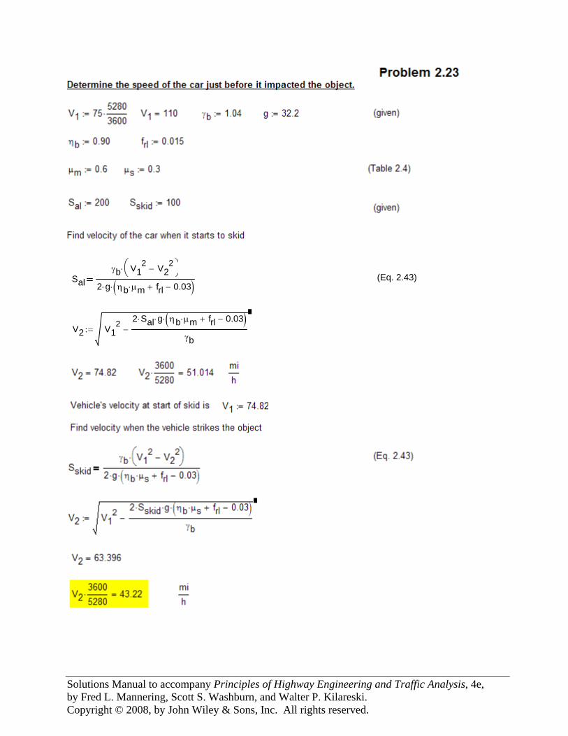
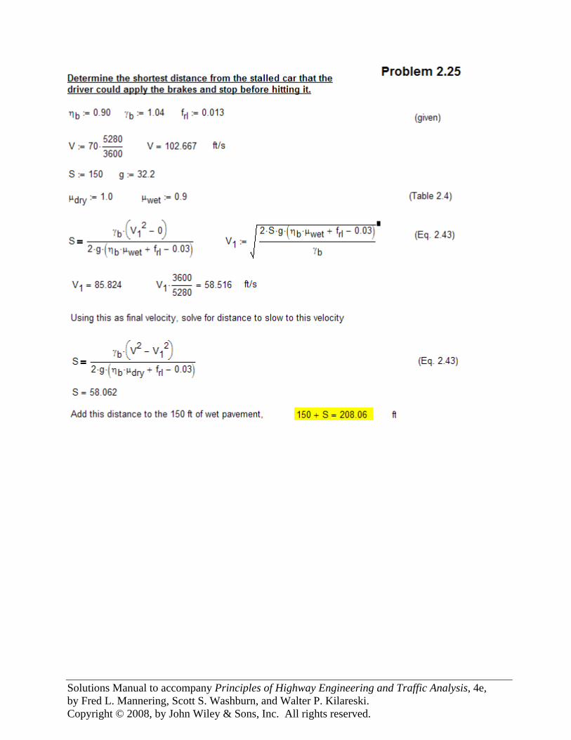
Salγb V1
2 V22
−⎛⎝
⎞⎠⋅
2 g⋅ ηb μm⋅ frl 0.03−+( )⋅(Eq. 2.43)
V2 V12 2 Sal⋅ g⋅ ηb μm⋅ frl+ 0.03−( )⋅
γb−:=
Solutions Manual to accompany Principles of Highway Engineering and Traffic Analysis, 4e, by Fred L. Mannering, Scott S. Washburn, and Walter P. Kilareski. Copyright © 2008, by John Wiley & Sons, Inc. All rights reserved.
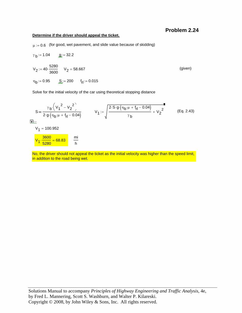
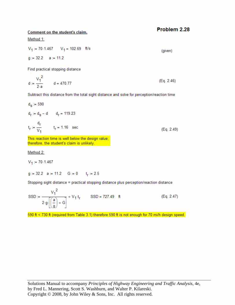
Problem 2.24 Determine if the driver should appeal the ticket.
μ 0.6:= (for good, wet pavement, and slide value because of skidding)
γ b 1.04:= g 32.2:=
V2 4052803600⋅:= V2 58.667= (given)
ηb 0.95:= S 200:= frl 0.015:=
Solve for the initial velocity of the car using theoretical stopping distance
Sγ b V1
2 V22
−⎛⎝
⎞⎠⋅
2 g⋅ ηb μ⋅ frl+ 0.04−( )⋅V1
2 S⋅ g⋅ ηb μ⋅ frl+ 0.04−( )⋅
γ bV2
2+:= (Eq. 2.43)
V1 100.952=
V136005280⋅ 68.83=
mih
No, the driver should not appeal the ticket as the initial velocity was higher than the speed limit,in addition to the road being wet.
Solutions Manual to accompany Principles of Highway Engineering and Traffic Analysis, 4e, by Fred L. Mannering, Scott S. Washburn, and Walter P. Kilareski. Copyright © 2008, by John Wiley & Sons, Inc. All rights reserved.
Solutions Manual to accompany Principles of Highway Engineering and Traffic Analysis, 4e, by Fred L. Mannering, Scott S. Washburn, and Walter P. Kilareski. Copyright © 2008, by John Wiley & Sons, Inc. All rights reserved.
Solutions Manual to accompany Principles of Highway Engineering and Traffic Analysis, 4e, by Fred L. Mannering, Scott S. Washburn, and Walter P. Kilareski. Copyright © 2008, by John Wiley & Sons, Inc. All rights reserved.
Solutions Manual to accompany Principles of Highway Engineering and Traffic Analysis, 4e, by Fred L. Mannering, Scott S. Washburn, and Walter P. Kilareski. Copyright © 2008, by John Wiley & Sons, Inc. All rights reserved.
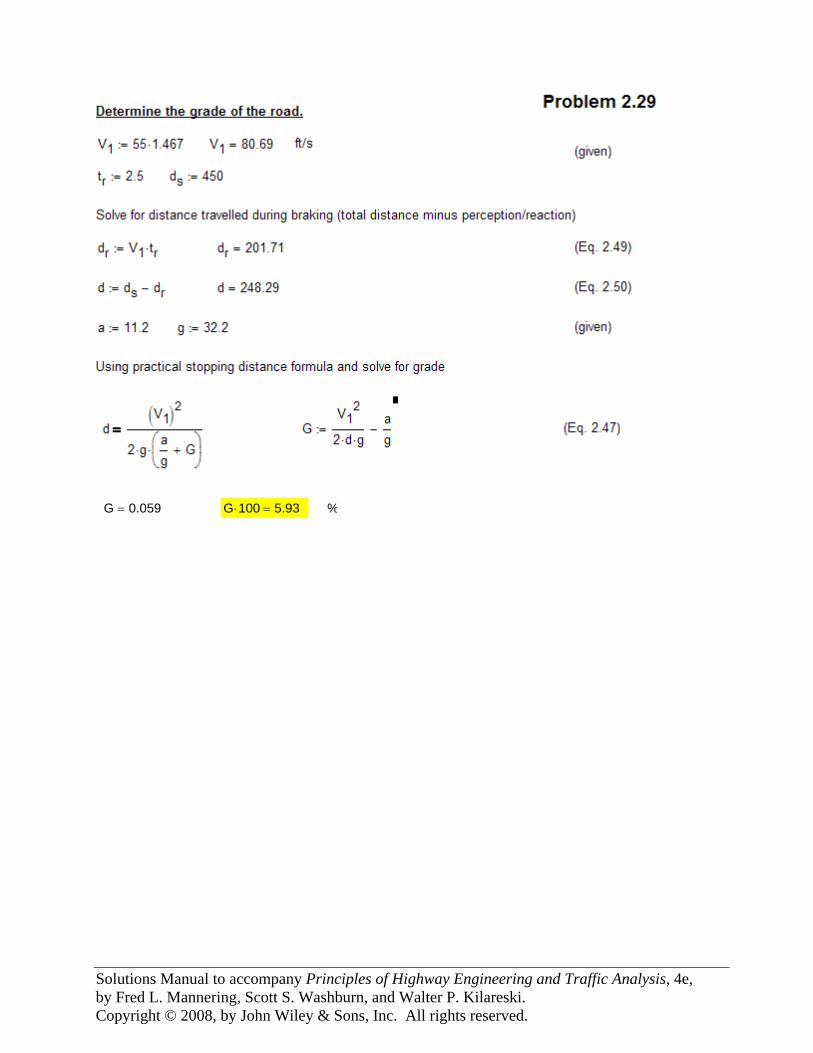
G 0.059= G 100⋅ 5.93= %
Solutions Manual to accompany Principles of Highway Engineering and Traffic Analysis, 4e, by Fred L. Mannering, Scott S. Washburn, and Walter P. Kilareski. Copyright © 2008, by John Wiley & Sons, Inc. All rights reserved.
Solutions Manual to accompany Principles of Highway Engineering and Traffic Analysis, 4e, by Fred L. Mannering, Scott S. Washburn, and Walter P. Kilareski. Copyright © 2008, by John Wiley & Sons, Inc. All rights reserved.
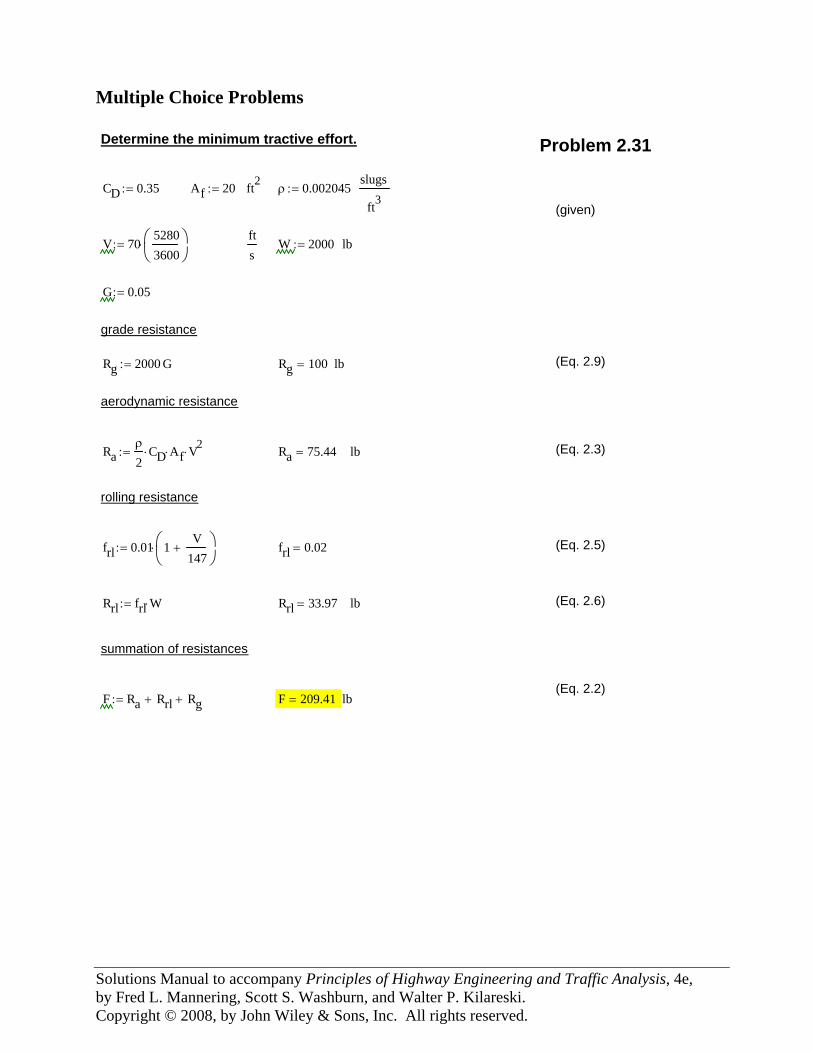
Multiple Choice Problems Determine the minimum tractive effort. Problem 2.31
CD 0.35:= Af 20:= ft2 ρ 0.002045:=slugs
ft3 (given)
V 7052803600
⎛⎜⎝
⎞⎟⎠
⋅:=fts
W 2000:= lb
G 0.05:=
grade resistance
Rg 2000 G⋅:= Rg 100= lb (Eq. 2.9)
aerodynamic resistance
Raρ
2CD⋅ Af⋅ V2
⋅:= Ra 75.44= lb (Eq. 2.3)
rolling resistance
frl 0.01 1V
147+⎛⎜
⎝⎞⎟⎠
⋅:= frl 0.02= (Eq. 2.5)
Rrl frl W⋅:= Rrl 33.97= lb (Eq. 2.6)
summation of resistances
(Eq. 2.2)F Ra Rrl+ Rg+:= F 209.41= lb
Solutions Manual to accompany Principles of Highway Engineering and Traffic Analysis, 4e, by Fred L. Mannering, Scott S. Washburn, and Walter P. Kilareski. Copyright © 2008, by John Wiley & Sons, Inc. All rights reserved.
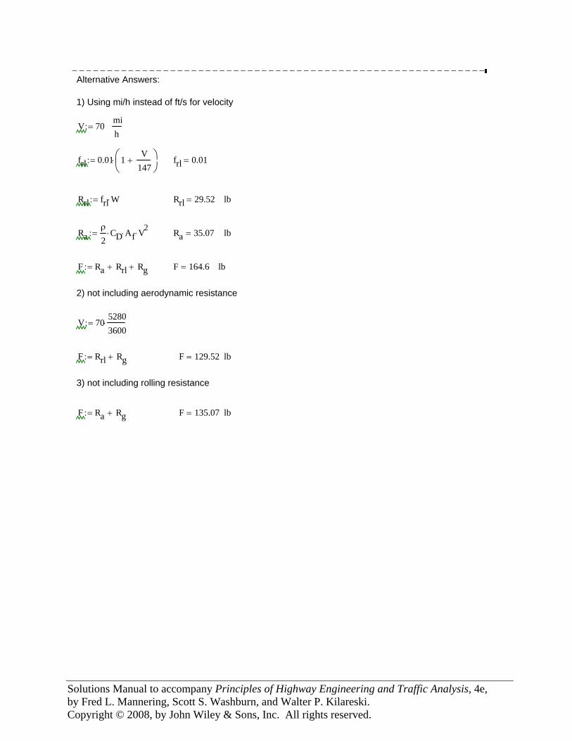
−−−−−−−−−−−−−−−−−−−−−−−−−−−−−−−−−−−−−−−−−−−−−−−−−−−−−−−−−−−Alternative Answers:
1) Using mi/h instead of ft/s for velocity
V 70:=mih
frl 0.01 1V
147+⎛⎜
⎝⎞⎟⎠
⋅:= frl 0.01=
Rrl frl W⋅:= Rrl 29.52= lb
Raρ
2CD⋅ Af⋅ V2
⋅:= Ra 35.07= lb
F Ra Rrl+ Rg+:= F 164.6= lb
2) not including aerodynamic resistance
V 7052803600⋅:=
F Rrl Rg+:= F 129.52= lb
3) not including rolling resistance
F Ra Rg+:= F 135.07= lb
Solutions Manual to accompany Principles of Highway Engineering and Traffic Analysis, 4e, by Fred L. Mannering, Scott S. Washburn, and Walter P. Kilareski. Copyright © 2008, by John Wiley & Sons, Inc. All rights reserved.
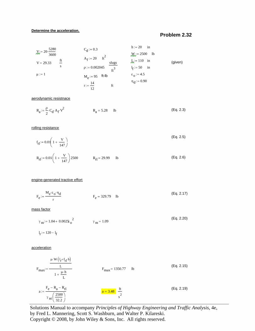
Determine the acceleration.Problem 2.32
h 20:= inCd 0.3:=V 2052803600⋅:= W 2500:= lb
Af 20:= ft2 L 110:= inV 29.33=fts
(given)slugs
ft3ρ 0.002045:= lf 50:= in
μ 1:= εo 4.5:=Me 95:= ft-lbηd 0.90:=
r1412
:= ft
aerodynamic resistnace
Raρ
2Cd⋅ Af⋅ V2
⋅:= Ra 5.28= lb (Eq. 2.3)
rolling resistance
(Eq. 2.5)frl 0.01 1
V147
+⎛⎜⎝
⎞⎟⎠
:=
Rrl 0.01 1V
147+⎛⎜
⎝⎞⎟⎠
⋅ 2500⋅:= Rrl 29.99= lb (Eq. 2.6)
engine-generated tractive effort
(Eq. 2.17)Fe
Me εo⋅ ηd⋅
r:= Fe 329.79= lb
mass factor
(Eq. 2.20)γ m 1.04 0.0025εo
2+:= γ m 1.09=
lr 120 lf−:=
acceleration
(Eq. 2.15)Fmax
μ W⋅ lr frl h⋅+( )⋅
L
1μ h⋅L
+
:= Fmax 1350.77= lb
(Eq. 2.19)a
Fe Ra− Rrl−
γ m250032.2
⎛⎜⎝
⎞⎟⎠
⋅
:= a 3.48=ft
s2
Solutions Manual to accompany Principles of Highway Engineering and Traffic Analysis, 4e, by Fred L. Mannering, Scott S. Washburn, and Walter P. Kilareski. Copyright © 2008, by John Wiley & Sons, Inc. All rights reserved.
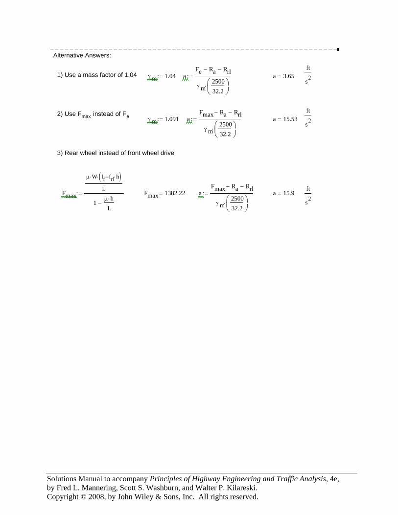
−−−−−−−−−−−−−−−−−−−−−−−−−−−−−−−−−−−−−−−−−−−−−−−−−−−−−−−−−−−Alternative Answers:
ft
s21) Use a mass factor of 1.04 γ m 1.04:= aFe Ra− Rrl−
γ m250032.2
⎛⎜⎝
⎞⎟⎠
⋅
:= a 3.65=
2) Use Fmax instead of Feft
s2γ m 1.091:= aFmax Ra− Rrl−
γ m250032.2
⎛⎜⎝
⎞⎟⎠
⋅
:= a 15.53=
3) Rear wheel instead of front wheel drive
Fmax
μ W⋅ lf frl h⋅−( )⋅
L
1μ h⋅L
−
:= Fmax 1382.22= aFmax Ra− Rrl−
γ m250032.2
⎛⎜⎝
⎞⎟⎠
⋅
:= a 15.9=ft
s2
Solutions Manual to accompany Principles of Highway Engineering and Traffic Analysis, 4e, by Fred L. Mannering, Scott S. Washburn, and Walter P. Kilareski. Copyright © 2008, by John Wiley & Sons, Inc. All rights reserved.
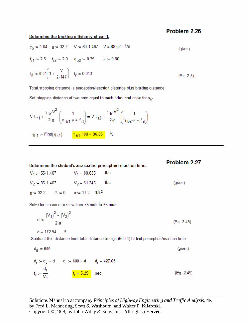
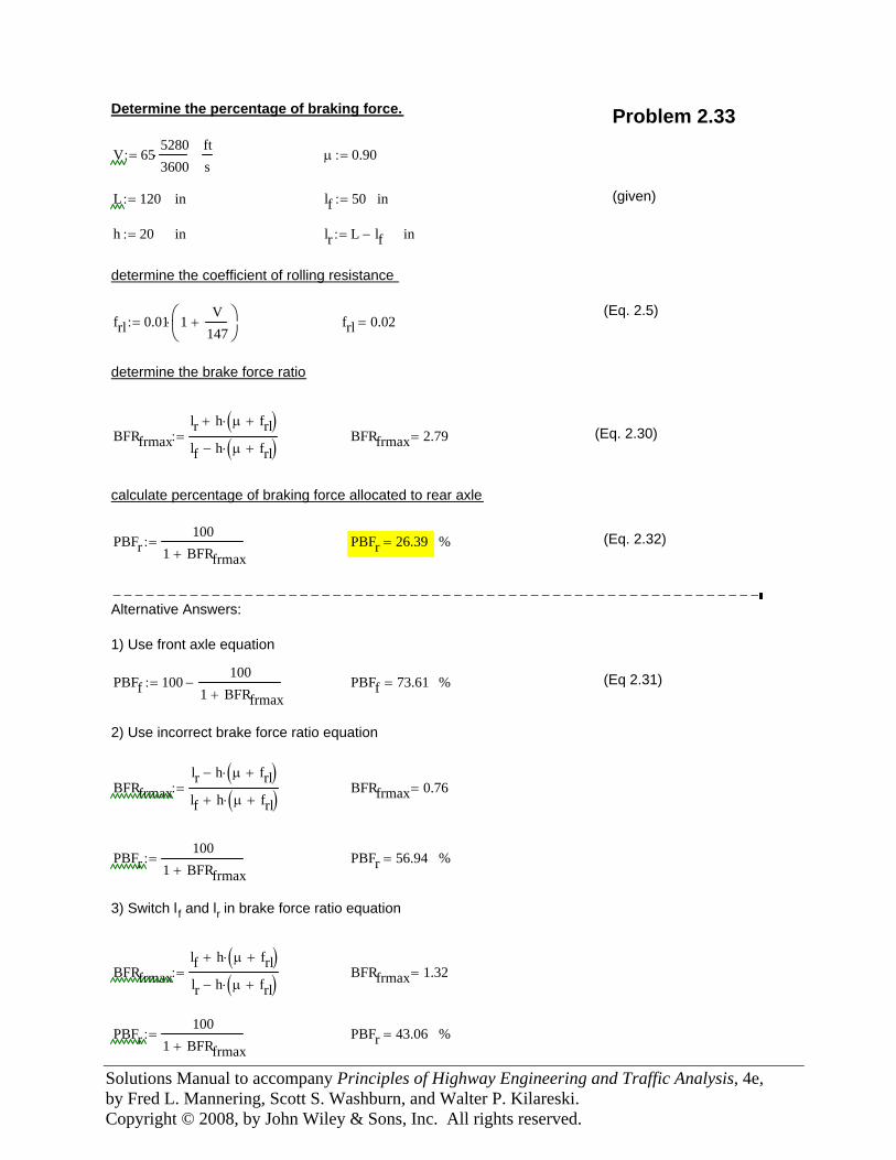
Determine the percentage of braking force. Problem 2.33
V 6552803600⋅:=
fts
μ 0.90:=
L 120:= in lf 50:= in (given)
h 20:= in lr L lf−:= in
determine the coefficient of rolling resistance
(Eq. 2.5)frl 0.01 1
V147
+⎛⎜⎝
⎞⎟⎠
⋅:= frl 0.02=
determine the brake force ratio
BFRfrmaxlr h μ frl+( )⋅+
lf h μ frl+( )⋅−:= BFRfrmax 2.79= (Eq. 2.30)
calculate percentage of braking force allocated to rear axle
PBFr100
1 BFRfrmax+:= PBFr 26.39= % (Eq. 2.32)
−−−−−−−−−−−−−−−−−−−−−−−−−−−−−−−−−−−−−−−−−−−−−−−−−−−−−−−−−−−Alternative Answers:
1) Use front axle equation
PBFf 100100
1 BFRfrmax+−:= PBFf 73.61= % (Eq 2.31)
2) Use incorrect brake force ratio equation
BFRfrmaxlr h μ frl+( )⋅−
lf h μ frl+( )⋅+:= BFRfrmax 0.76=
PBFr100
1 BFRfrmax+:= PBFr 56.94= %
3) Switch l f and lr in brake force ratio equation
BFRfrmaxlf h μ frl+( )⋅+
lr h μ frl+( )⋅−:= BFRfrmax 1.32=
PBFr100
1 BFRfrmax+:= PBFr 43.06= %
Solutions Manual to accompany Principles of Highway Engineering and Traffic Analysis, 4e, by Fred L. Mannering, Scott S. Washburn, and Walter P. Kilareski. Copyright © 2008, by John Wiley & Sons, Inc. All rights reserved.
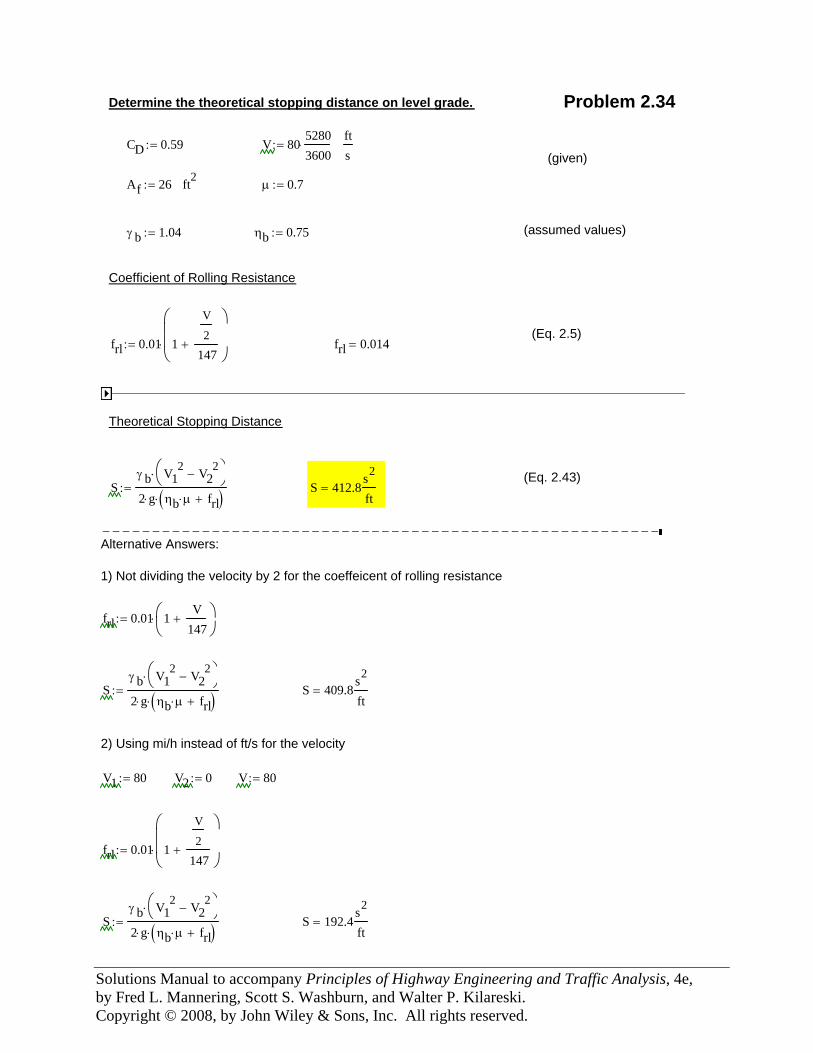
Determine the theoretical stopping distance on level grade. Problem 2.34
CD 0.59:= V 8052803600⋅:=
fts (given)
Af 26:= ft2 μ 0.7:=
γ b 1.04:= ηb 0.75:= (assumed values)
Coefficient of Rolling Resistance
(Eq. 2.5) frl 0.01 1
V
2
147+
⎛⎜⎜⎝
⎞⎟⎟⎠
⋅:= frl 0.014=
Theoretical Stopping Distance
(Eq. 2.43)S
γ b V12 V2
2−⎛
⎝⎞⎠⋅
2 g⋅ ηb μ⋅ frl+( )⋅:= S 412.8
s2
ft=
−−−−−−−−−−−−−−−−−−−−−−−−−−−−−−−−−−−−−−−−−−−−−−−−−−−−−−−−
Alternative Answers:
1) Not dividing the velocity by 2 for the coeffeicent of rolling resistance
frl 0.01 1V
147+⎛⎜
⎝⎞⎟⎠
⋅:=
Sγ b V1
2 V22
−⎛⎝
⎞⎠⋅
2 g⋅ ηb μ⋅ frl+( )⋅:= S 409.8
s2
ft=
2) Using mi/h instead of ft/s for the velocity
V1 80:= V2 0:= V 80:=
frl 0.01 1
V
2
147+
⎛⎜⎜⎝
⎞⎟⎟⎠
⋅:=
Sγ b V1
2 V22
−⎛⎝
⎞⎠⋅
2 g⋅ ηb μ⋅ frl+( )⋅:= S 192.4
s2
ft=
Solutions Manual to accompany Principles of Highway Engineering and Traffic Analysis, 4e, by Fred L. Mannering, Scott S. Washburn, and Walter P. Kilareski. Copyright © 2008, by John Wiley & Sons, Inc. All rights reserved.
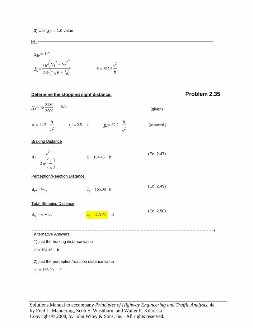
3) Using γ = 1.0 value
γ b 1.0:=
Sγ b V1
2 V22
−⎛⎝
⎞⎠⋅
2 g⋅ ηb μ⋅ frl+( )⋅:= S 397.9
s2
ft=
Determine the stopping sight distance. Problem 2.35
V 4552803600⋅:= ft/s (given)
a 11.2:=ft
s2tr 2.5:= s g 32.2:=
ft
s2assumed( )
Braking Distance
(Eq. 2.47)d
V2
2 g⋅ag
⎛⎜⎝
⎞⎟⎠
⋅
:= d 194.46= ft
Perception/Reaction Distance
(Eq. 2.49)dr V tr⋅:= dr 165.00= ft
Total Stopping Distance
(Eq. 2.50)ds d dr+:= ds 359.46= ft
−−−−−−−−−−−−−−−−−−−−−−−−−−−−−−−−−−−−−−−−−−−−−−−−−−−−−−−−−−−Alternative Answers:
1) just the braking distance value
d 194.46= ft
2) just the perception/reaction distance value
dr 165.00= ft
Solutions Manual to accompany Principles of Highway Engineering and Traffic Analysis, 4e, by Fred L. Mannering, Scott S. Washburn, and Walter P. Kilareski. Copyright © 2008, by John Wiley & Sons, Inc. All rights reserved.
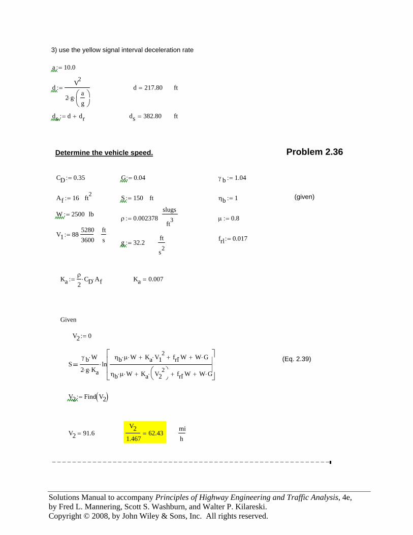
3) use the yellow signal interval deceleration rate
a 10.0:=
dV2
2 g⋅ag
⎛⎜⎝
⎞⎟⎠
⋅
:= d 217.80= ft
ds d dr+:= ds 382.80= ft
Determine the vehicle speed. Problem 2.36
CD 0.35:= G 0.04:= γ b 1.04:=
Af 16:= ft2 S 150:= ft ηb 1:= (given)
W 2500:= lbslugs
ft3ρ 0.002378:= μ 0.8:=
V1 8852803600⋅:=
fts frl 0.017:=g 32.2:=
ft
s2
Kaρ
2CD⋅ Af⋅:= Ka 0.007=
Given
V2 0:=
(Eq. 2.39)S
γ b W⋅
2 g⋅ Ka⋅ln
ηb μ⋅ W⋅ Ka V12
⋅+ frl W⋅+ W G⋅+
ηb μ⋅ W⋅ Ka V22⎛
⎝⎞⎠⋅+ frl W⋅+ W G⋅+
⎡⎢⎢⎣
⎤⎥⎥⎦
⋅
V2 Find V2( ):=
V2 91.6=V2
1.46762.43=
mih
−−−−−−−−−−−−−−−−−−−−−−−−−−−−−−−−−−−−−−−−−−−−−−−−−−−−−−−
Solutions Manual to accompany Principles of Highway Engineering and Traffic Analysis, 4e, by Fred L. Mannering, Scott S. Washburn, and Walter P. Kilareski. Copyright © 2008, by John Wiley & Sons, Inc. All rights reserved.
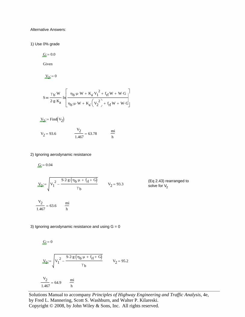
−−−−−−−−−−−−−−−−−−−−−−−−−−−−−−−−−−−−−−−−−−−−−−−−−−−−−Alternative Answers:
1) Use 0% grade
G 0.0:=
Given
V2 0:=
Sγ b W⋅
2 g⋅ Ka⋅ln
ηb μ⋅ W⋅ Ka V12
⋅+ frl W⋅+ W G⋅+
ηb μ⋅ W⋅ Ka V22⎛
⎝⎞⎠⋅+ frl W⋅+ W G⋅+
⎡⎢⎢⎣
⎤⎥⎥⎦
⋅
V2 Find V2( ):=
V2 93.6=V2
1.46763.78=
mih
2) Ignoring aerodynamic resistance
G 0.04:=
(Eq 2.43) rearranged tosolve for V2
V2 V12 S 2⋅ g⋅ ηb μ⋅ frl+ G+( )⋅
γ b−:= V2 93.3=
V21.467
63.6=mih
3) Ignoring aerodynamic resistance and using G = 0
G 0:=
V2 V12 S 2⋅ g⋅ ηb μ⋅ frl+ G+( )⋅
γ b−:= V2 95.2=
V21.467
64.9=mih
Solutions Manual to accompany
Principles of Highway Engineering and Traffic Analysis, 4e
By Fred L. Mannering, Scott S. Washburn, and Walter P. Kilareski
Chapter 3 Geometric Design of Highways
U.S. Customary Units
Copyright © 2008, by John Wiley & Sons, Inc. All rights reserved.

Solutions Manual to accompany Principles of Highway Engineering and Traffic Analysis, 4e, by Fred L. Mannering, Scott S. Washburn, and Walter P. Kilareski. Copyright © 2008, by John Wiley & Sons, Inc. All rights reserved.
Preface The solutions to the fourth edition of Principles of Highway Engineering and Traffic Analysis were prepared with the Mathcad1 software program. You will notice several notation conventions that you may not be familiar with if you are not a Mathcad user. Most of these notation conventions are self-explanatory or easily understood. The most common Mathcad specific notations in these solutions relate to the equals sign. You will notice the equals sign being used in three different contexts, and Mathcad uses three different notations to distinguish between each of these contexts. The differences between these equals sign notations are explained as follows.
• The ‘:=’ (colon-equals) is an assignment operator, that is, the value of the variable or expression on the left side of ‘:=’is set equal to the value of the expression on the right side. For example, in the statement, L := 1234, the variable ‘L’ is assigned (i.e., set equal to) the value of 1234. Another example is x := y + z. In this case, x is assigned the value of y + z.
• The ‘==’ (bold equals) is used when the Mathcad function solver was used to find the value of a variable in the equation. For example, in the equation
, the == is used to tell Mathcad that the value of the expression on the left side needs to equal the value of the expression on the right side. Thus, the Mathcad solver can be employed to find a value for the variable ‘t’ that satisfies this relationship. This particular example is from a problem where the function for arrivals at some time ‘t’ is set equal to the function for departures at some time ‘t’ to find the time to queue clearance.
• The ‘=’ (standard equals) is used for a simple numeric evaluation. For example, referring to the x := y + z assignment used previously, if the value of y was 10 [either by assignment (with :=), or the result of an equation solution (through the use of ==) and the value of z was 15, then the expression ‘x =’ would yield 25. Another example would be as follows: s := 1800/3600, with s = 0.5. That is, ‘s’ was assigned the value of 1800 divided by 3600 (using :=), which equals 0.5 (as given by using =).
Another symbol you will see frequently is ‘→’. In these solutions, it is used to perform an evaluation of an assignment expression in a single statement. For example, in the following
statement, , Q(t) is assigned the value of Arrivals(t) – Departures(t), and this evaluates to 2.2t – 0.10t2. Finally, to assist in quickly identifying the final answer, or answers, for what is being asked in the problem statement, yellow highlighting has been used (which will print as light gray). 1 www.mathcad.com
Solutions Manual to accompany Principles of Highway Engineering and Traffic Analysis, 4e, by Fred L. Mannering, Scott S. Washburn, and Walter P. Kilareski. Copyright © 2008, by John Wiley & Sons, Inc. All rights reserved.
Solutions Manual to accompany Principles of Highway Engineering and Traffic Analysis, 4e, by Fred L. Mannering, Scott S. Washburn, and Walter P. Kilareski. Copyright © 2008, by John Wiley & Sons, Inc. All rights reserved.
Solutions Manual to accompany Principles of Highway Engineering and Traffic Analysis, 4e, by Fred L. Mannering, Scott S. Washburn, and Walter P. Kilareski. Copyright © 2008, by John Wiley & Sons, Inc. All rights reserved.
Solutions Manual to accompany Principles of Highway Engineering and Traffic Analysis, 4e, by Fred L. Mannering, Scott S. Washburn, and Walter P. Kilareski. Copyright © 2008, by John Wiley & Sons, Inc. All rights reserved.
Solutions Manual to accompany Principles of Highway Engineering and Traffic Analysis, 4e, by Fred L. Mannering, Scott S. Washburn, and Walter P. Kilareski. Copyright © 2008, by John Wiley & Sons, Inc. All rights reserved.
Solutions Manual to accompany Principles of Highway Engineering and Traffic Analysis, 4e, by Fred L. Mannering, Scott S. Washburn, and Walter P. Kilareski. Copyright © 2008, by John Wiley & Sons, Inc. All rights reserved.
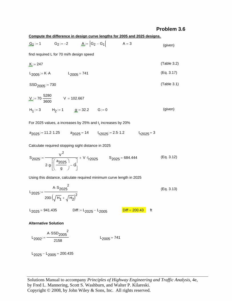
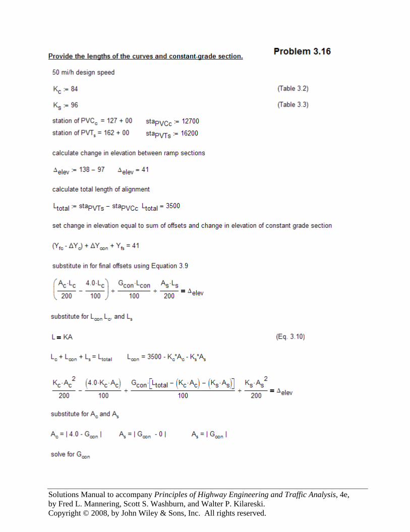
Problem 3.6 Compute the difference in design curve lengths for 2005 and 2025 designs.
G1 1:= G2 2−:= A G2 G1−:= A 3= (given)
find required L for 70 mi/h design speed
K 247:= (Table 3.2)
L2005 K A⋅:= L2005 741= (Eq. 3.17)
SSD2005 730:= (Table 3.1)
V 7052803600⋅:= V 102.667=
H1 3:= H2 1:= g 32.2:= G 0:= (given)
For 2025 values, a increases by 25% and tr increases by 20%
a2025 11.2 1.25⋅:= a2025 14= tr2025 2.5 1.2⋅:= tr2025 3=
Calculate required stopping sight distance in 2025
S2025V 2
2 g⋅a2025
g
⎛⎜⎝
⎞⎟⎠
G−⎡⎢⎣
⎤⎥⎦
⋅
V tr2025⋅+:= S2025 684.444= (Eq. 3.12)
Using this distance, calculate required minimum curve length in 2025
(Eq. 3.13)L2025
A S20252
⋅
200 H1 H2+( )2⋅
:=
L2025 941.435= Diff L2025 L2005−:= Diff 200.43= ft
Alternative Solution
L2002A SSD2005
2⋅
2158:= L2005 741=
L2025 L2005− 200.435=
Solutions Manual to accompany Principles of Highway Engineering and Traffic Analysis, 4e, by Fred L. Mannering, Scott S. Washburn, and Walter P. Kilareski. Copyright © 2008, by John Wiley & Sons, Inc. All rights reserved.
Solutions Manual to accompany Principles of Highway Engineering and Traffic Analysis, 4e, by Fred L. Mannering, Scott S. Washburn, and Walter P. Kilareski. Copyright © 2008, by John Wiley & Sons, Inc. All rights reserved.
Solutions Manual to accompany Principles of Highway Engineering and Traffic Analysis, 4e, by Fred L. Mannering, Scott S. Washburn, and Walter P. Kilareski. Copyright © 2008, by John Wiley & Sons, Inc. All rights reserved.
Solutions Manual to accompany Principles of Highway Engineering and Traffic Analysis, 4e, by Fred L. Mannering, Scott S. Washburn, and Walter P. Kilareski. Copyright © 2008, by John Wiley & Sons, Inc. All rights reserved.
Solutions Manual to accompany Principles of Highway Engineering and Traffic Analysis, 4e, by Fred L. Mannering, Scott S. Washburn, and Walter P. Kilareski. Copyright © 2008, by John Wiley & Sons, Inc. All rights reserved.
Solutions Manual to accompany Principles of Highway Engineering and Traffic Analysis, 4e, by Fred L. Mannering, Scott S. Washburn, and Walter P. Kilareski. Copyright © 2008, by John Wiley & Sons, Inc. All rights reserved.
Solutions Manual to accompany Principles of Highway Engineering and Traffic Analysis, 4e, by Fred L. Mannering, Scott S. Washburn, and Walter P. Kilareski. Copyright © 2008, by John Wiley & Sons, Inc. All rights reserved.
Solutions Manual to accompany Principles of Highway Engineering and Traffic Analysis, 4e, by Fred L. Mannering, Scott S. Washburn, and Walter P. Kilareski. Copyright © 2008, by John Wiley & Sons, Inc. All rights reserved.
Solutions Manual to accompany Principles of Highway Engineering and Traffic Analysis, 4e, by Fred L. Mannering, Scott S. Washburn, and Walter P. Kilareski. Copyright © 2008, by John Wiley & Sons, Inc. All rights reserved.
Solutions Manual to accompany Principles of Highway Engineering and Traffic Analysis, 4e, by Fred L. Mannering, Scott S. Washburn, and Walter P. Kilareski. Copyright © 2008, by John Wiley & Sons, Inc. All rights reserved.
Solutions Manual to accompany Principles of Highway Engineering and Traffic Analysis, 4e, by Fred L. Mannering, Scott S. Washburn, and Walter P. Kilareski. Copyright © 2008, by John Wiley & Sons, Inc. All rights reserved.
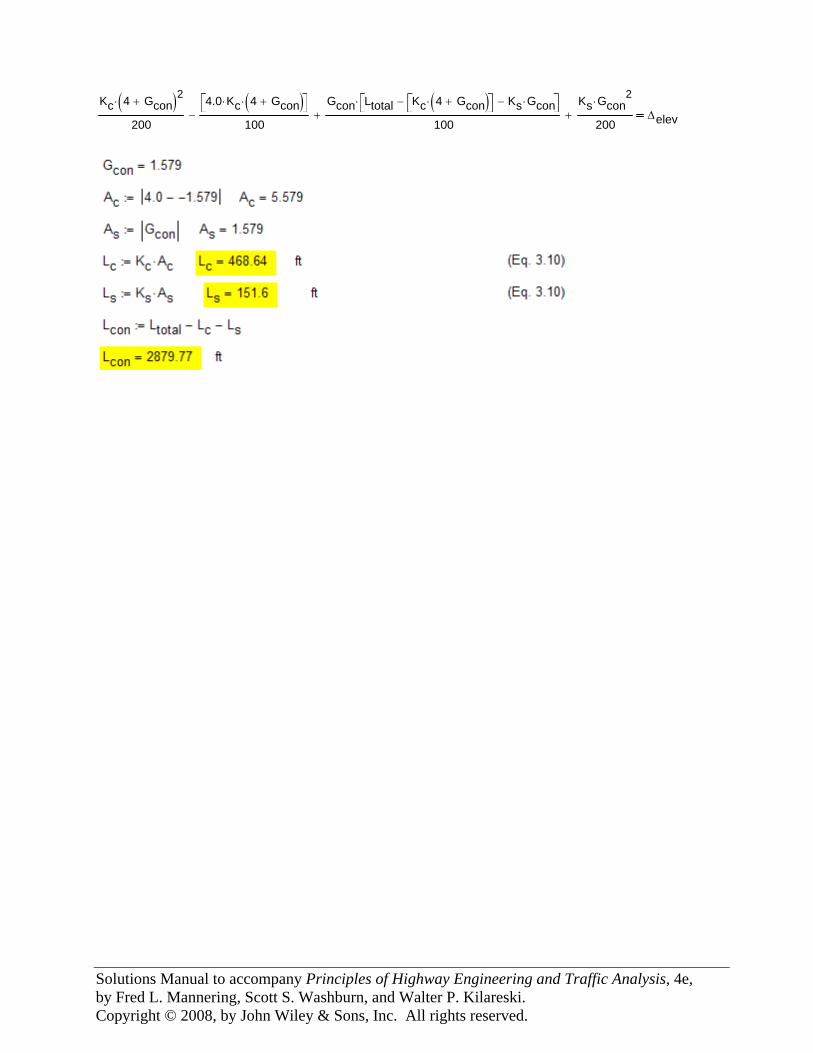
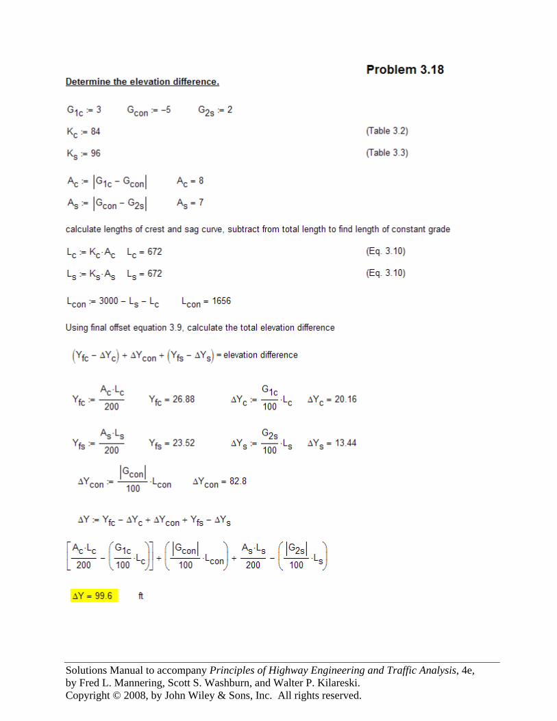
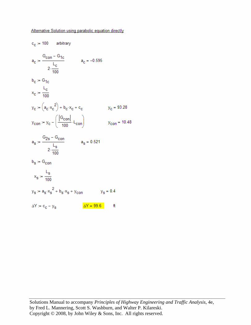
Kc 4 Gcon+( )2⋅
200
4.0 Kc⋅ 4 Gcon+( )⋅⎡⎣ ⎤⎦100
−Gcon Ltotal Kc 4 Gcon+( )⋅⎡⎣ ⎤⎦− Ks Gcon⋅−⎡⎣ ⎤⎦⋅
100+
Ks Gcon2
⋅
200+ Δelev
Solutions Manual to accompany Principles of Highway Engineering and Traffic Analysis, 4e, by Fred L. Mannering, Scott S. Washburn, and Walter P. Kilareski. Copyright © 2008, by John Wiley & Sons, Inc. All rights reserved.
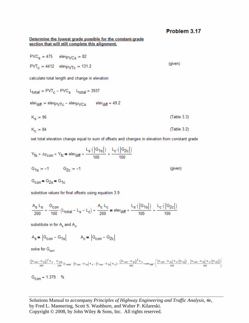
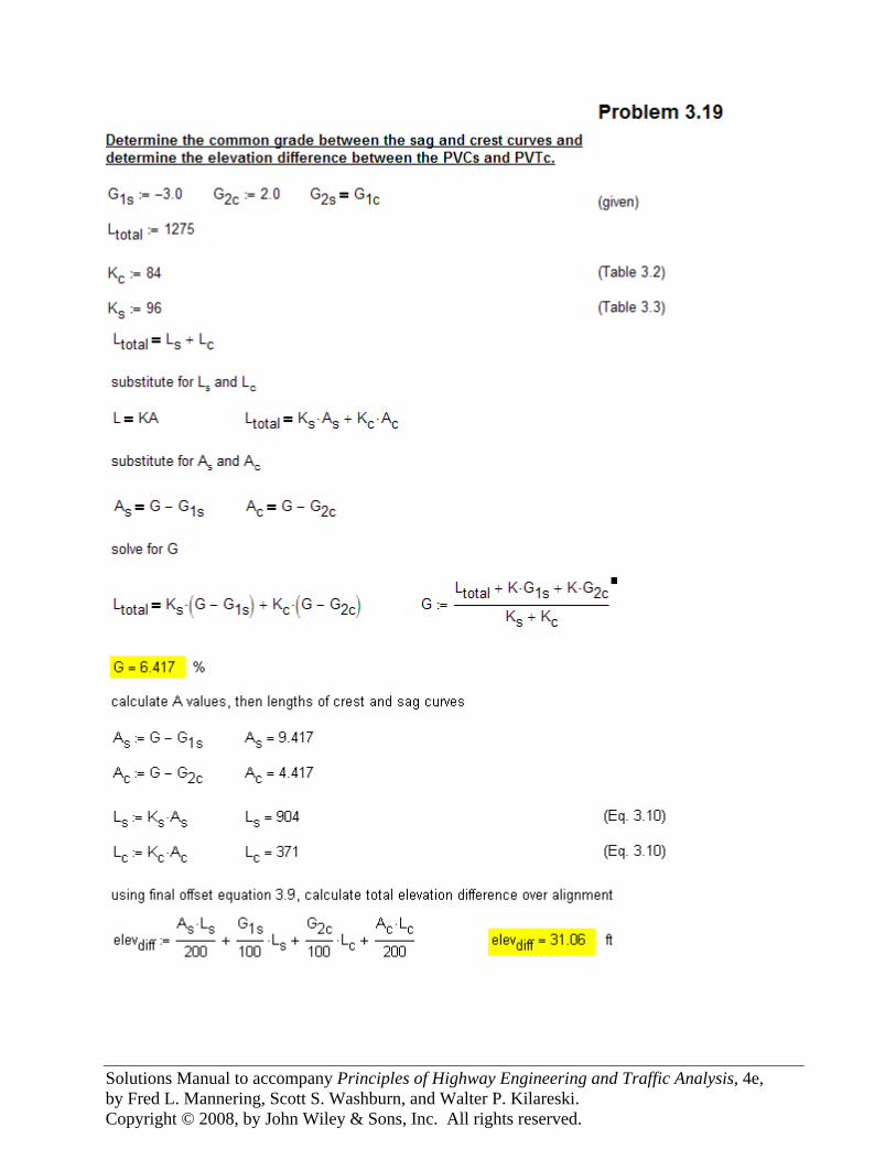
G con G 1s−( )2 K s⋅
200
G con100
L total G con G 1s− K s⋅− G con G 2c− K c⋅−( )⋅+G con G 2c−( )2 K c⋅
200+ elev diff
G con G 1s− K s⋅ G 1s( )⋅
100
G con G 2c− K c⋅ G 2c( )⋅
100+
⎡⎢⎣
⎤⎥⎦
+
Solutions Manual to accompany Principles of Highway Engineering and Traffic Analysis, 4e, by Fred L. Mannering, Scott S. Washburn, and Walter P. Kilareski. Copyright © 2008, by John Wiley & Sons, Inc. All rights reserved.
Solutions Manual to accompany Principles of Highway Engineering and Traffic Analysis, 4e, by Fred L. Mannering, Scott S. Washburn, and Walter P. Kilareski. Copyright © 2008, by John Wiley & Sons, Inc. All rights reserved.
Solutions Manual to accompany Principles of Highway Engineering and Traffic Analysis, 4e, by Fred L. Mannering, Scott S. Washburn, and Walter P. Kilareski. Copyright © 2008, by John Wiley & Sons, Inc. All rights reserved.
Solutions Manual to accompany Principles of Highway Engineering and Traffic Analysis, 4e, by Fred L. Mannering, Scott S. Washburn, and Walter P. Kilareski. Copyright © 2008, by John Wiley & Sons, Inc. All rights reserved.
Solutions Manual to accompany Principles of Highway Engineering and Traffic Analysis, 4e, by Fred L. Mannering, Scott S. Washburn, and Walter P. Kilareski. Copyright © 2008, by John Wiley & Sons, Inc. All rights reserved.
Solutions Manual to accompany Principles of Highway Engineering and Traffic Analysis, 4e, by Fred L. Mannering, Scott S. Washburn, and Walter P. Kilareski. Copyright © 2008, by John Wiley & Sons, Inc. All rights reserved.
Solutions Manual to accompany Principles of Highway Engineering and Traffic Analysis, 4e, by Fred L. Mannering, Scott S. Washburn, and Walter P. Kilareski. Copyright © 2008, by John Wiley & Sons, Inc. All rights reserved.
Solutions Manual to accompany Principles of Highway Engineering and Traffic Analysis, 4e, by Fred L. Mannering, Scott S. Washburn, and Walter P. Kilareski. Copyright © 2008, by John Wiley & Sons, Inc. All rights reserved.
Solutions Manual to accompany Principles of Highway Engineering and Traffic Analysis, 4e, by Fred L. Mannering, Scott S. Washburn, and Walter P. Kilareski. Copyright © 2008, by John Wiley & Sons, Inc. All rights reserved.
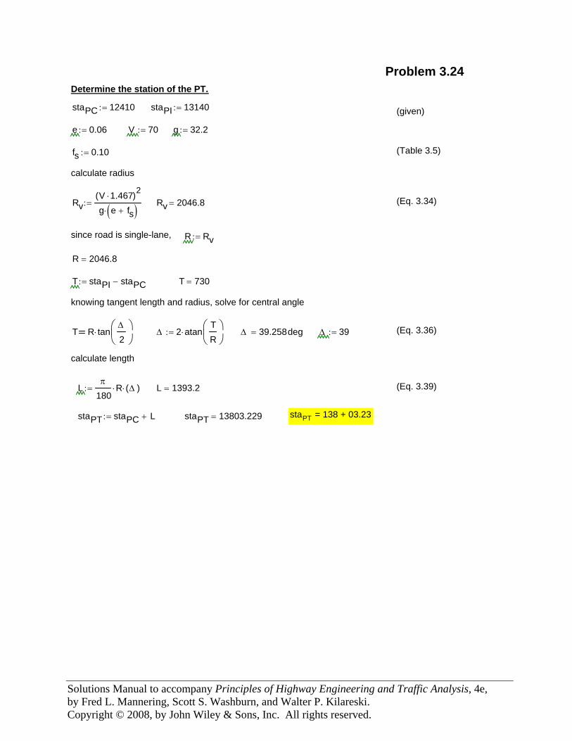
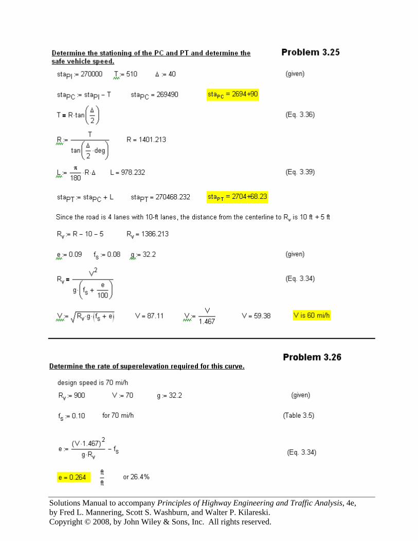
Problem 3.24 Determine the station of the PT.
staPC 12410:= staPI 13140:= (given)
e 0.06:= V 70:= g 32.2:=
fs 0.10:= (Table 3.5)
calculate radius
RvV 1.467⋅( )2
g e fs+( )⋅:= Rv 2046.8= (Eq. 3.34)
since road is single-lane, R Rv:=
R 2046.8=
T staPI staPC−:= T 730=
knowing tangent length and radius, solve for central angle
T R tanΔ
2⎛⎜⎝
⎞⎟⎠
⋅ Δ 2 atanTR
⎛⎜⎝
⎞⎟⎠
⋅:= Δ 39.258deg= Δ 39:= (Eq. 3.36)
calculate length
Lπ
180R⋅ Δ( )⋅:= L 1393.2= (Eq. 3.39)
staPT staPC L+:= staPT 13803.229= staPT = 138 + 03.23
Solutions Manual to accompany Principles of Highway Engineering and Traffic Analysis, 4e, by Fred L. Mannering, Scott S. Washburn, and Walter P. Kilareski. Copyright © 2008, by John Wiley & Sons, Inc. All rights reserved.
Solutions Manual to accompany Principles of Highway Engineering and Traffic Analysis, 4e, by Fred L. Mannering, Scott S. Washburn, and Walter P. Kilareski. Copyright © 2008, by John Wiley & Sons, Inc. All rights reserved.
Solutions Manual to accompany Principles of Highway Engineering and Traffic Analysis, 4e, by Fred L. Mannering, Scott S. Washburn, and Walter P. Kilareski. Copyright © 2008, by John Wiley & Sons, Inc. All rights reserved.
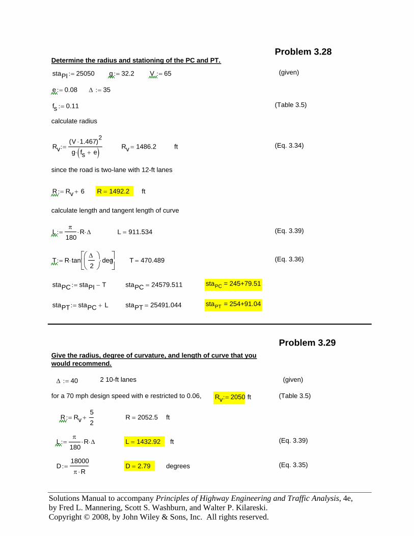
Problem 3.28 Determine the radius and stationing of the PC and PT.
staPI 25050:= g 32.2:= V 65:= (given)
e 0.08:= Δ 35:=
fs 0.11:= (Table 3.5)
calculate radius
RvV 1.467⋅( )2
g fs e+( )⋅:= Rv 1486.2= ft (Eq. 3.34)
since the road is two-lane with 12-ft lanes
R Rv 6+:= R 1492.2= ft
calculate length and tangent length of curve
Lπ
180R⋅ Δ⋅:= L 911.534= (Eq. 3.39)
T R tanΔ
2⎛⎜⎝
⎞⎟⎠
deg⋅⎡⎢⎣
⎤⎥⎦
⋅:= T 470.489= (Eq. 3.36)
staPC staPI T−:= staPC 24579.511= staPC = 245+79.51
staPT staPC L+:= staPT 25491.044= staPT = 254+91.04
Problem 3.29 Give the radius, degree of curvature, and length of curve that youwould recommend.
Δ 40:= 2 10-ft lanes (given)
for a 70 mph design speed with e restricted to 0.06, Rv 2050:= ft (Table 3.5)
R Rv52
+:= R 2052.5= ft
Lπ
180R⋅ Δ⋅:= L 1432.92= ft (Eq. 3.39)
D18000π R⋅
:= D 2.79= degrees (Eq. 3.35)
Solutions Manual to accompany Principles of Highway Engineering and Traffic Analysis, 4e, by Fred L. Mannering, Scott S. Washburn, and Walter P. Kilareski. Copyright © 2008, by John Wiley & Sons, Inc. All rights reserved.
Solutions Manual to accompany Principles of Highway Engineering and Traffic Analysis, 4e, by Fred L. Mannering, Scott S. Washburn, and Walter P. Kilareski. Copyright © 2008, by John Wiley & Sons, Inc. All rights reserved.
Solutions Manual to accompany Principles of Highway Engineering and Traffic Analysis, 4e, by Fred L. Mannering, Scott S. Washburn, and Walter P. Kilareski. Copyright © 2008, by John Wiley & Sons, Inc. All rights reserved.
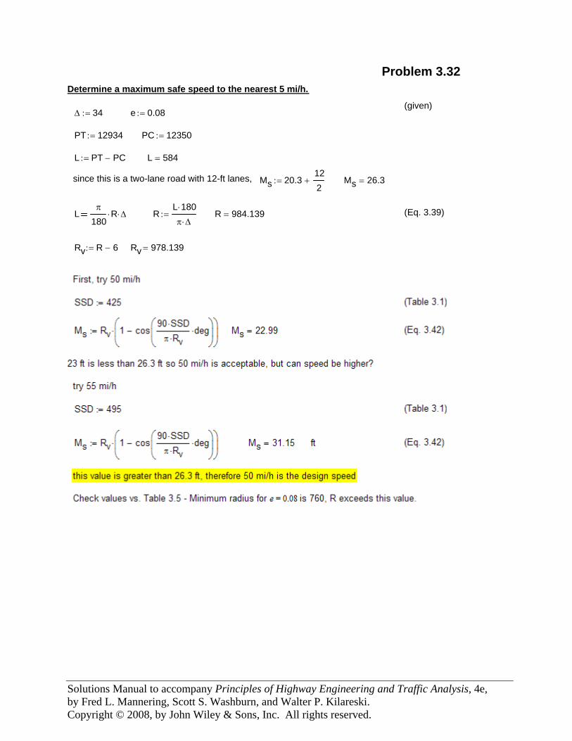
Rv 978.139=Rv R 6−:=
(Eq. 3.39)R 984.139=RL 180⋅
π Δ⋅:=L
π
180R⋅ Δ⋅
Ms 26.3=Ms 20.3122
+:=since this is a two-lane road with 12-ft lanes,
L 584=L PT PC−:=
PC 12350:=PT 12934:=
e 0.08:=Δ 34:=(given)
Determine a maximum safe speed to the nearest 5 mi/h.
Problem 3.32
Solutions Manual to accompany Principles of Highway Engineering and Traffic Analysis, 4e, by Fred L. Mannering, Scott S. Washburn, and Walter P. Kilareski. Copyright © 2008, by John Wiley & Sons, Inc. All rights reserved.
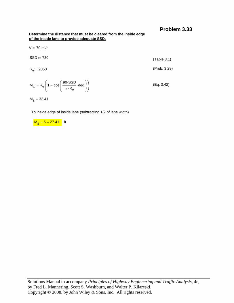
Problem 3.33 Determine the distance that must be cleared from the inside edgeof the inside lane to provide adequate SSD.
V is 70 mi/h
SSD 730:= (Table 3.1)
Rv 2050:= (Prob. 3.29)
Ms Rv 1 cos90 SSD⋅
π Rv⋅deg⋅
⎛⎜⎝
⎞⎟⎠
−⎛⎜⎝
⎞⎟⎠
⋅:= (Eq. 3.42)
Ms 32.41=
To inside edge of inside lane (subtracting 1/2 of lane width)
Ms 5− 27.41= ft
Solutions Manual to accompany Principles of Highway Engineering and Traffic Analysis, 4e, by Fred L. Mannering, Scott S. Washburn, and Walter P. Kilareski. Copyright © 2008, by John Wiley & Sons, Inc. All rights reserved.
Solutions Manual to accompany Principles of Highway Engineering and Traffic Analysis, 4e, by Fred L. Mannering, Scott S. Washburn, and Walter P. Kilareski. Copyright © 2008, by John Wiley & Sons, Inc. All rights reserved.
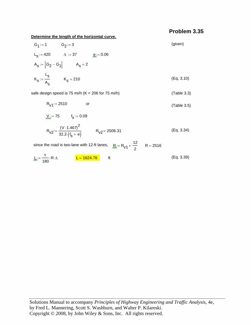
Problem 3.35 Determine the length of the horizontal curve.
G1 1:= G2 3:= (given)
Ls 420:= Δ 37:= e 0.06:=
As G2 G1−:= As 2=
KsLsAs
:= Ks 210= (Eq. 3.10)
safe design speed is 75 mi/h (K = 206 for 75 mi/h) (Table 3.3)
Rv1 2510:= or (Table 3.5)
V 75:= fs 0.09:=
Rv2V 1.467⋅( )2
32.2 fs e+( )⋅:= Rv2 2506.31= (Eq. 3.34)
since the road is two-lane with 12-ft lanes, R Rv1122
+:= R 2516=
Lπ
180R⋅ Δ⋅:= L 1624.76= ft (Eq. 3.39)
Solutions Manual to accompany Principles of Highway Engineering and Traffic Analysis, 4e, by Fred L. Mannering, Scott S. Washburn, and Walter P. Kilareski. Copyright © 2008, by John Wiley & Sons, Inc. All rights reserved.
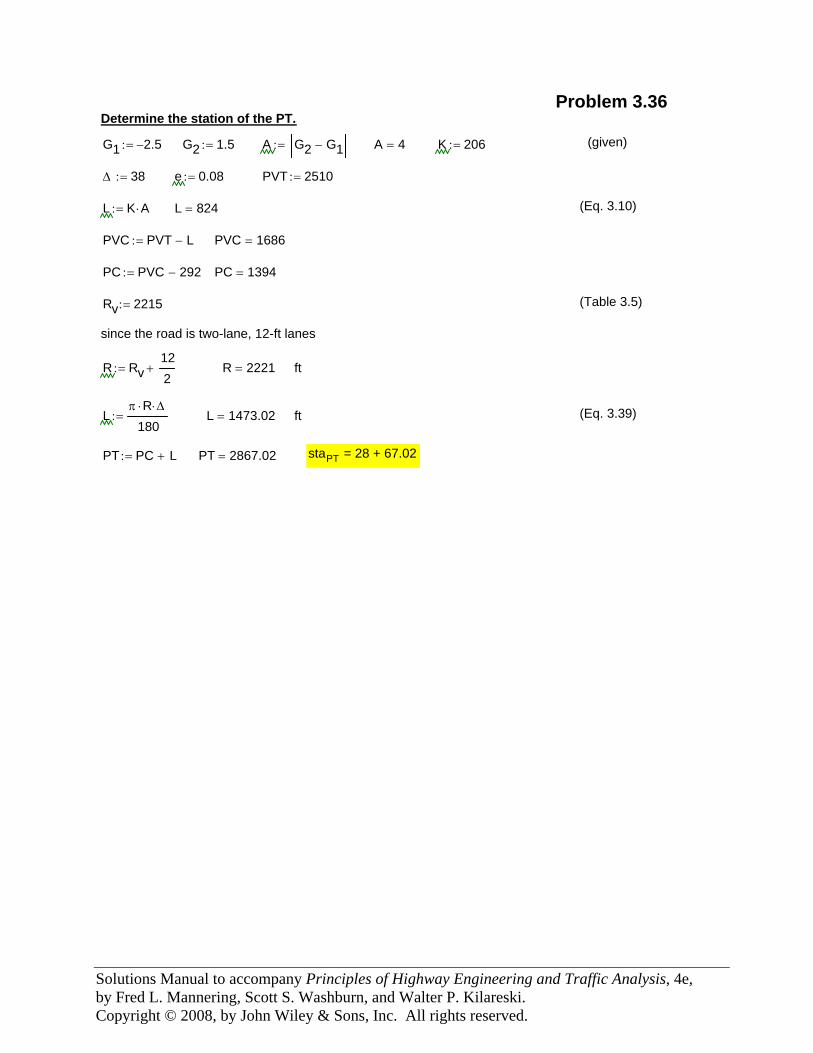
Problem 3.36 Determine the station of the PT.
G1 2.5−:= G2 1.5:= A G2 G1−:= A 4= K 206:= (given)
Δ 38:= e 0.08:= PVT 2510:=
L K A⋅:= L 824= (Eq. 3.10)
PVC PVT L−:= PVC 1686=
PC PVC 292−:= PC 1394=
Rv 2215:= (Table 3.5)
since the road is two-lane, 12-ft lanes
R Rv122
+:= R 2221= ft
Lπ R⋅ Δ⋅
180:= L 1473.02= ft (Eq. 3.39)
PT PC L+:= PT 2867.02= staPT = 28 + 67.02
Solutions Manual to accompany Principles of Highway Engineering and Traffic Analysis, 4e, by Fred L. Mannering, Scott S. Washburn, and Walter P. Kilareski. Copyright © 2008, by John Wiley & Sons, Inc. All rights reserved.
Solutions Manual to accompany Principles of Highway Engineering and Traffic Analysis, 4e, by Fred L. Mannering, Scott S. Washburn, and Walter P. Kilareski. Copyright © 2008, by John Wiley & Sons, Inc. All rights reserved.
Solutions Manual to accompany Principles of Highway Engineering and Traffic Analysis, 4e, by Fred L. Mannering, Scott S. Washburn, and Walter P. Kilareski. Copyright © 2008, by John Wiley & Sons, Inc. All rights reserved.
Multiple Choice Problems
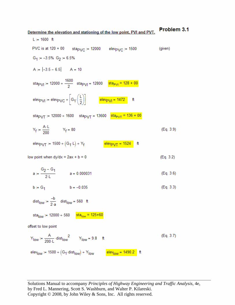
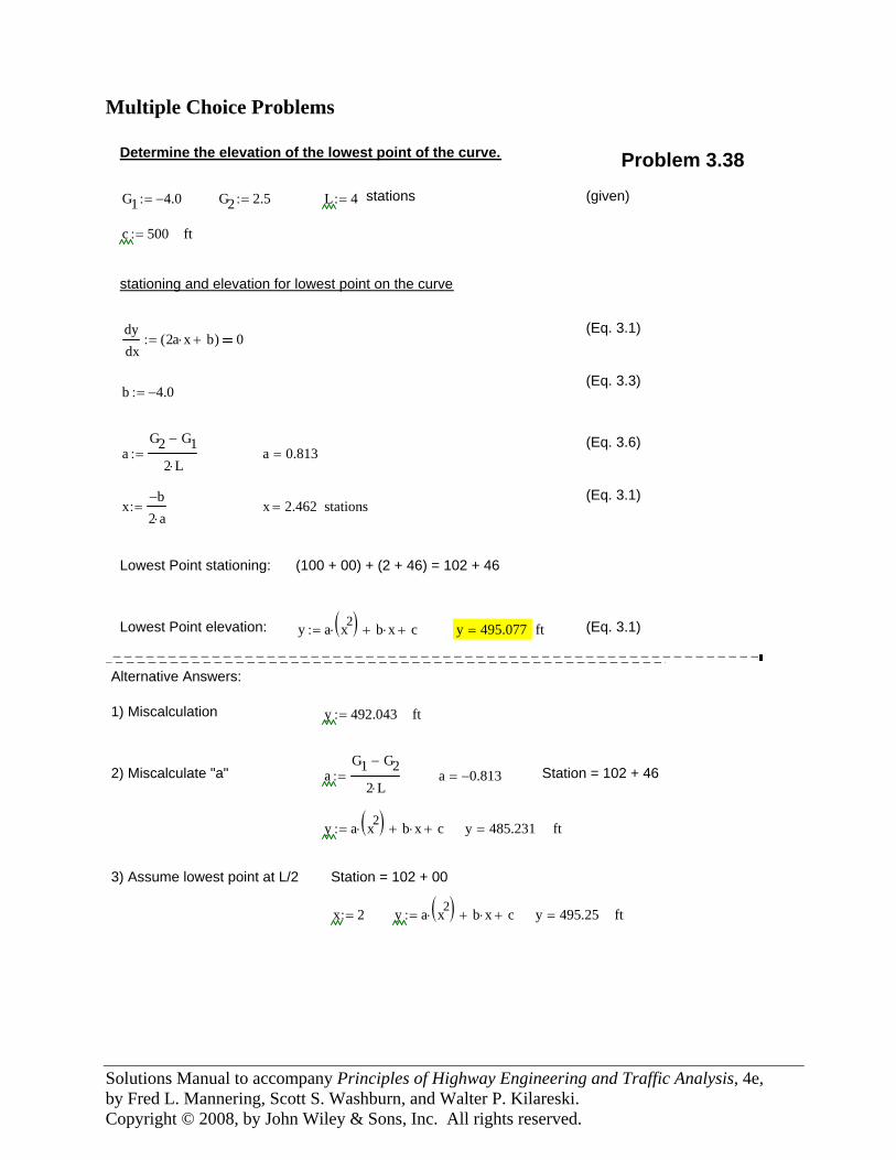
Determine the elevation of the lowest point of the curve. Problem 3.38
G1 4.0−:= G2 2.5:= L 4:= stations (given)
c 500:= ft
stationing and elevation for lowest point on the curve
(Eq. 3.1)dydx
2a x⋅ b+( ):= 0
(Eq. 3.3)b 4.0−:=
(Eq. 3.6)a
G2 G1−
2 L⋅:= a 0.813=
(Eq. 3.1)x
b−2 a⋅
:= x 2.462= stations
Lowest Point stationing: (100 + 00) + (2 + 46) = 102 + 46
Lowest Point elevation: y a x2( )⋅ b x⋅+ c+:= y 495.077= ft (Eq. 3.1)
−−−−−−−−−−−−−−−−−−−−−−−−−−−−−−−−−−−−−−−−−−−−−−−−−−−−−−−−−−− −−−−−−−−−−−−−−−−−−−−−−−−−−−−−−−−−−−−−−−−−−−−−−−−−−−−Alternative Answers:
1) Miscalculation y 492.043:= ft
2) Miscalculate "a" aG1 G2−
2 L⋅:= a 0.813−= Station = 102 + 46
y a x2( )⋅ b x⋅+ c+:= y 485.231= ft 3) Assume lowest point at L/2 Station = 102 + 00
x 2:= y a x2( )⋅ b x⋅+ c+:= y 495.25= ft
Solutions Manual to accompany Principles of Highway Engineering and Traffic Analysis, 4e, by Fred L. Mannering, Scott S. Washburn, and Walter P. Kilareski. Copyright © 2008, by John Wiley & Sons, Inc. All rights reserved.
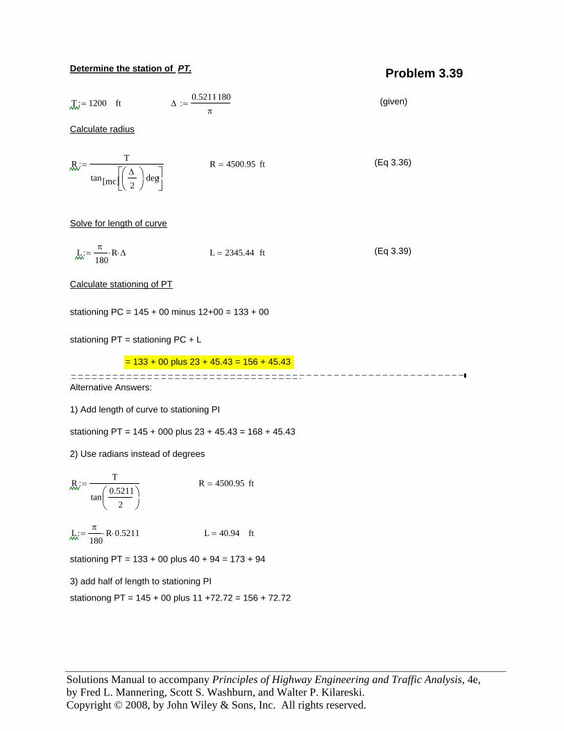
Determine the station of PT. Problem 3.39
T 1200:= ft Δ0.5211180⋅
π:= (given)
Calculate radius
RT
tan[mc]Δ
2⎛⎜⎝
⎞⎟⎠
deg⋅⎡⎢⎣
⎤⎥⎦
:= R 4500.95= ft (Eq 3.36)
Solve for length of curve
Lπ
180R⋅ Δ⋅:= L 2345.44= ft (Eq 3.39)
Calculate stationing of PT
stationing PC = 145 + 00 minus 12+00 = 133 + 00
stationing PT = stationing PC + L
= 133 + 00 plus 23 + 45.43 = 156 + 45.43−−−−−−−−−−−−−−−−−−−−−−−−−−−−−−−−−−−−−−−−−−−−−−−−−−−−−−−−− −−−−−−−−−−−−−−−−−−−−−−−−−−−−−−−−−−
Alternative Answers:
1) Add length of curve to stationing PI
stationing PT = 145 + 000 plus 23 + 45.43 = 168 + 45.43
2) Use radians instead of degrees
RT
tan0.5211
2⎛⎜⎝
⎞⎟⎠
:= R 4500.95= ft
Lπ
180R⋅ 0.5211⋅:= L 40.94= ft
stationing PT = 133 + 00 plus 40 + 94 = 173 + 94
3) add half of length to stationing PI
stationong PT = 145 + 00 plus 11 +72.72 = 156 + 72.72
Solutions Manual to accompany Principles of Highway Engineering and Traffic Analysis, 4e, by Fred L. Mannering, Scott S. Washburn, and Walter P. Kilareski. Copyright © 2008, by John Wiley & Sons, Inc. All rights reserved.
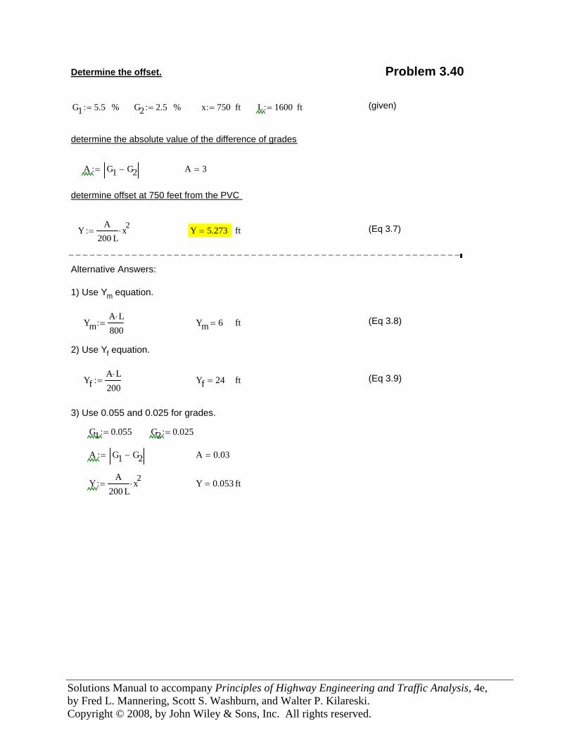
Determine the offset. Problem 3.40
G1 5.5:= % G2 2.5:= % x 750:= ft L 1600:= ft (given)
determine the absolute value of the difference of grades
A G1 G2−:= A 3=
determine offset at 750 feet from the PVC
YA
200 L⋅x2⋅:= Y 5.273= ft (Eq 3.7)
−−−−−−−−−−−−−−−−−−−−−−−−−−−−−−−−−−−−−−−−−−−−−−−−−−−−−−−−
Alternative Answers:
1) Use Ym equation.
YmA L⋅800
:= Ym 6= ft (Eq 3.8)
2) Use Yf equation.
YfA L⋅200
:= Yf 24= ft (Eq 3.9)
3) Use 0.055 and 0.025 for grades.
G1 0.055:= G2 0.025:=
A G1 G2−:= A 0.03=
YA
200 L⋅x2⋅:= Y 0.053= ft
Solutions Manual to accompany Principles of Highway Engineering and Traffic Analysis, 4e, by Fred L. Mannering, Scott S. Washburn, and Walter P. Kilareski. Copyright © 2008, by John Wiley & Sons, Inc. All rights reserved.
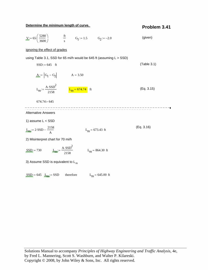
Determine the minimum length of curve. Problem 3.41
V 6552803600
⎛⎜⎝
⎞⎟⎠
⋅:=fts
G1 1.5:= G2 2.0−:= (given)
ignoring the effect of grades
using Table 3.1, SSD for 65 mi/h would be 645 ft (assuming L > SSD)
SSD 645:= ft (Table 3.1)
A G1 G2−:= A 3.50=
LmA SSD2⋅
2158:= Lm 674.74= ft (Eq. 3.15)
674.74 645> −−−−−−−−−−−−−−−−−−−−−−−−−−−−−−−−−−−−−−−−−−−−−−−−−−−−−−−−− −−−−−−−−−−−−−−−−−−−−−−−−−−−−−−−−−−−−−−−−−−−−−−−−−−
Alternative Answers
1) assume L < SSD
(Eq. 3.16)Lm 2 SSD⋅
2158A
−:= Lm 673.43= ft
2) Misinterpret chart for 70 mi/h
SSD 730:= LmA SSD2⋅
2158:= Lm 864.30= ft
3) Assume SSD is equivalent to Lm
SSD 645:= Lm SSD:= therefore Lm 645.00= ft
Solutions Manual to accompany Principles of Highway Engineering and Traffic Analysis, 4e, by Fred L. Mannering, Scott S. Washburn, and Walter P. Kilareski. Copyright © 2008, by John Wiley & Sons, Inc. All rights reserved.
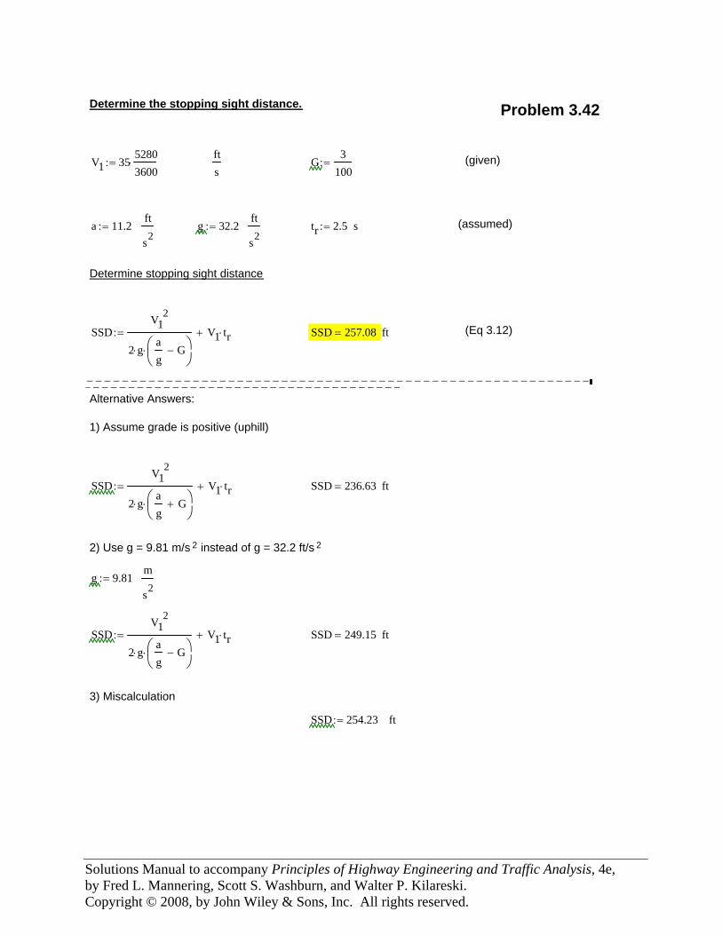
Determine the stopping sight distance. Problem 3.42
V1 3552803600⋅:=
fts
G3
100:= (given)
a 11.2:=ft
s2g 32.2:=
ft
s2tr 2.5:= s (assumed)
Determine stopping sight distance
SSDV1
2
2 g⋅ag
G−⎛⎜⎝
⎞⎟⎠
⋅
V1 tr⋅+:= SSD 257.08= ft (Eq 3.12)
−−−−−−−−−−−−−−−−−−−−−−−−−−−−−−−−−−−−−−−−−−−−−−−−−−−−−−−−− −−−−−−−−−−−−−−−−−−−−−−−−−−−−−−−−−−−−
Alternative Answers:
1) Assume grade is positive (uphill)
SSDV1
2
2 g⋅ag
G+⎛⎜⎝
⎞⎟⎠
⋅
V1 tr⋅+:= SSD 236.63= ft
2) Use g = 9.81 m/s 2 instead of g = 32.2 ft/s 2
g 9.81:=m
s2
SSDV1
2
2 g⋅ag
G−⎛⎜⎝
⎞⎟⎠
⋅
V1 tr⋅+:= SSD 249.15= ft
3) Miscalculation
SSD 254.23:= ft
Solutions Manual to accompany Principles of Highway Engineering and Traffic Analysis, 4e, by Fred L. Mannering, Scott S. Washburn, and Walter P. Kilareski. Copyright © 2008, by John Wiley & Sons, Inc. All rights reserved.
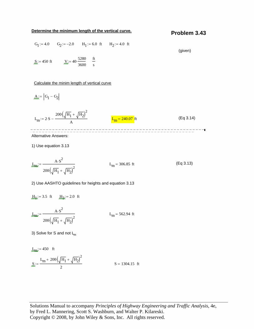
Determine the minimum length of the vertical curve. Problem 3.43
G1 4.0:= G2 2.0−:= H1 6.0:= ft H2 4.0:= ft
(given)
S 450:= ft V 4052803600⋅:=
fts
Calculate the minim length of vertical curve
A G1 G2−:=
Lm 2 S⋅200 H1 H2+( )2⋅
A−:= Lm 240.07= ft (Eq 3.14)
−−−−−−−−−−−−−−−−−−−−−−−−−−−−−−−−−−−−−−−−−−−−−−−−−−−−−−−− −−−−−−−−−−−−−−−−−−−−−−−−−−−−−−−−−−−−−−−−−−−−−−−−−−−−−
Alternative Answers:
1) Use equation 3.13
LmA S2⋅
200 H1 H2+( )2⋅
:= Lm 306.85= ft (Eq 3.13)
2) Use AASHTO guidelines for heights and equation 3.13
H1 3.5:= ft H2 2.0:= ft
LmA S2⋅
200 H1 H2+( )2⋅
:= Lm 562.94= ft
3) Solve for S and not Lm
Lm 450:= ft
SLm 200 H1 H2+( )2⋅+
2:= S 1304.15= ft
Solutions Manual to accompany
Principles of Highway Engineering and Traffic Analysis, 4e
By Fred L. Mannering, Scott S. Washburn, and Walter P. Kilareski
Chapter 4 Pavement Design
U.S. Customary Units
Copyright © 2008, by John Wiley & Sons, Inc. All rights reserved.

Solutions Manual to accompany Principles of Highway Engineering and Traffic Analysis, 4e, by Fred L. Mannering, Scott S. Washburn, and Walter P. Kilareski. Copyright © 2008, by John Wiley & Sons, Inc. All rights reserved.
Preface The solutions to the fourth edition of Principles of Highway Engineering and Traffic Analysis were prepared with the Mathcad1 software program. You will notice several notation conventions that you may not be familiar with if you are not a Mathcad user. Most of these notation conventions are self-explanatory or easily understood. The most common Mathcad specific notations in these solutions relate to the equals sign. You will notice the equals sign being used in three different contexts, and Mathcad uses three different notations to distinguish between each of these contexts. The differences between these equals sign notations are explained as follows.
• The ‘:=’ (colon-equals) is an assignment operator, that is, the value of the variable or expression on the left side of ‘:=’is set equal to the value of the expression on the right side. For example, in the statement, L := 1234, the variable ‘L’ is assigned (i.e., set equal to) the value of 1234. Another example is x := y + z. In this case, x is assigned the value of y + z.
• The ‘==’ (bold equals) is used when the Mathcad function solver was used to find the value of a variable in the equation. For example, in the equation
, the == is used to tell Mathcad that the value of the expression on the left side needs to equal the value of the expression on the right side. Thus, the Mathcad solver can be employed to find a value for the variable ‘t’ that satisfies this relationship. This particular example is from a problem where the function for arrivals at some time ‘t’ is set equal to the function for departures at some time ‘t’ to find the time to queue clearance.
• The ‘=’ (standard equals) is used for a simple numeric evaluation. For example, referring to the x := y + z assignment used previously, if the value of y was 10 [either by assignment (with :=), or the result of an equation solution (through the use of ==) and the value of z was 15, then the expression ‘x =’ would yield 25. Another example would be as follows: s := 1800/3600, with s = 0.5. That is, ‘s’ was assigned the value of 1800 divided by 3600 (using :=), which equals 0.5 (as given by using =).
Another symbol you will see frequently is ‘→’. In these solutions, it is used to perform an evaluation of an assignment expression in a single statement. For example, in the following
statement, , Q(t) is assigned the value of Arrivals(t) – Departures(t), and this evaluates to 2.2t – 0.10t2. Finally, to assist in quickly identifying the final answer, or answers, for what is being asked in the problem statement, yellow highlighting has been used (which will print as light gray). 1 www.mathcad.com
Solutions Manual to accompany Principles of Highway Engineering and Traffic Analysis, 4e, by Fred L. Mannering, Scott S. Washburn, and Walter P. Kilareski. Copyright © 2008, by John Wiley & Sons, Inc. All rights reserved.
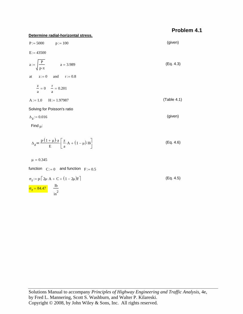
Solving for Poisson's ratio
Δz 0.016:= (given)
Find μ:
Δzp 1 μ+( )⋅ a⋅
Eza
A⋅ 1 μ−( ) H⋅+⎡⎢⎣
⎤⎥⎦
⋅ (Eq. 4.6)
μ 0.345=
function C 0:= and function F 0.5:=
σr p 2μ A⋅ C+ 1 2μ−( )F+⎡⎣ ⎤⎦⋅:= (Eq. 4.5)
σr 84.47=lb
in2
Problem 4.1Determine radial-horizontal stress.
P 5000:= p 100:= (given)
E 43500:=
aP
p π⋅:= a 3.989= (Eq. 4.3)
at z 0:= and r 0.8:=
za
0=ra
0.201=
A 1.0:= H 1.97987:= (Table 4.1)
Solutions Manual to accompany Principles of Highway Engineering and Traffic Analysis, 4e, by Fred L. Mannering, Scott S. Washburn, and Walter P. Kilareski. Copyright © 2008, by John Wiley & Sons, Inc. All rights reserved.
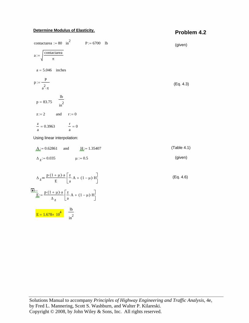
Determine Modulus of Elasticity. Problem 4.2
contactarea 80:= in2 P 6700:= lb (given)
acontactarea
π:=
a 5.046= inches
pP
a2π⋅
:= (Eq. 4.3)
lb
in2p 83.75=
z 2:= and r 0:=
za
0.3963=ra
0=
Using linear interpolation:
A 0.62861:= and H 1.35407:= (Table 4.1)
Δ z 0.035:= μ 0.5:= (given)
Δ zp 1 μ+( )⋅ a⋅
Eza
A⋅ 1 μ−( ) H⋅+⎡⎢⎣
⎤⎥⎦
⋅ (Eq. 4.6)
Ep 1 μ+( )⋅ a⋅
Δ z
za
A⋅ 1 μ−( ) H⋅+⎡⎢⎣
⎤⎥⎦
⋅:=
lb
in2E 1.678 104×=
Solutions Manual to accompany Principles of Highway Engineering and Traffic Analysis, 4e, by Fred L. Mannering, Scott S. Washburn, and Walter P. Kilareski. Copyright © 2008, by John Wiley & Sons, Inc. All rights reserved.
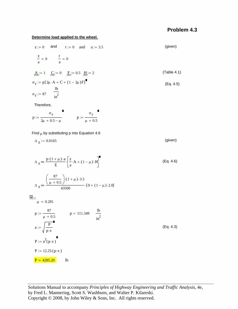
Problem 4.3Determine load applied to the wheel.
z 0:= and r 0:= and a 3.5:= (given)
za
0=ra
0=
A 1:= C 0:= F 0.5:= H 2:= (Table 4.1)
σr p 2μ A⋅ C+ 1 2μ−( )F+[ ]:= (Eq. 4.5)lb
in2σr 87:=
Therefore,
pσr
2μ 0.5+ μ−:= p
σrμ 0.5+
:=
Find μ by substituting p into Equation 4.6
Δ z 0.0165:= (given)
Δ zp 1 μ+( )⋅ a⋅
Eza
A⋅ 1 μ−( ) H⋅+⎡⎢⎣
⎤⎥⎦
⋅ (Eq. 4.6)
Δ z
87μ 0.5+
⎛⎜⎝⎞⎟⎠
1 μ+( )⋅ 3.5⋅
435000 1 μ−( ) 2.0⋅+[ ]⋅
μ 0.281=
p87
μ 0.5+:= p 111.349=
lb
in2
aP
p π⋅:= (Eq. 4.3)
P a2 p π⋅( ):=
P 12.25 p π⋅( )⋅:=
P 4285.20= lb
Solutions Manual to accompany Principles of Highway Engineering and Traffic Analysis, 4e, by Fred L. Mannering, Scott S. Washburn, and Walter P. Kilareski. Copyright © 2008, by John Wiley & Sons, Inc. All rights reserved.
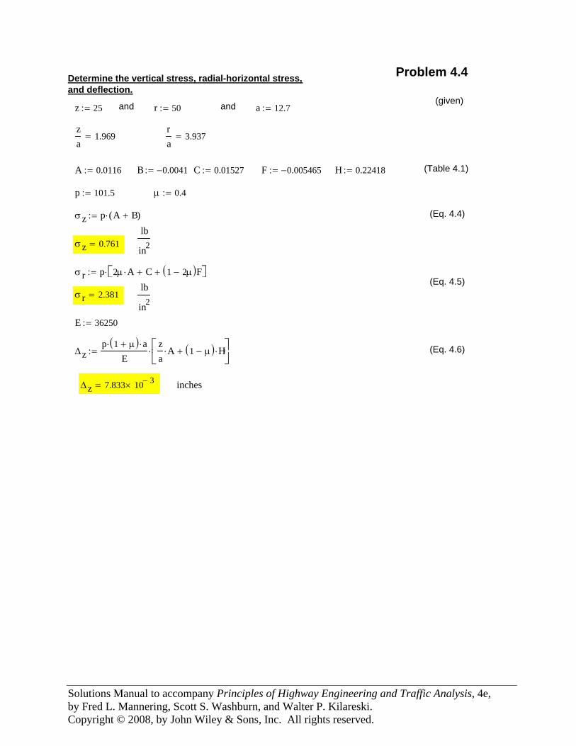
inchesΔz 7.833 10 3−×=
(Eq. 4.6)Δzp 1 μ+( )⋅ a⋅
Eza
A⋅ 1 μ−( ) H⋅+⎡⎢⎣
⎤⎥⎦
⋅:=
E 36250:=
lb
in2σ r 2.381=
(Eq. 4.5)σ r p 2μ A⋅ C+ 1 2μ−( )F+⎡⎣ ⎤⎦⋅:=
σz 0.761=lb
in2
(Eq. 4.4)σz p A B+( )⋅:=
μ 0.4:=p 101.5:=
(Table 4.1)H 0.22418:=F 0.005465−:=C 0.01527:=B 0.0041−:=A 0.0116:=
ra
3.937=za
1.969=
a 12.7:=andr 50:=and z 25:=(given)
Determine the vertical stress, radial-horizontal stress,and deflection.
Problem 4.4
Solutions Manual to accompany Principles of Highway Engineering and Traffic Analysis, 4e, by Fred L. Mannering, Scott S. Washburn, and Walter P. Kilareski. Copyright © 2008, by John Wiley & Sons, Inc. All rights reserved.
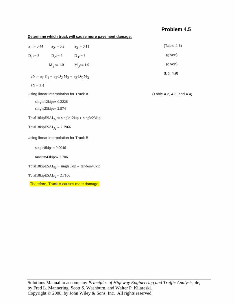
Therefore, Truck A causes more damage.
Total18kipESALB 2.7106=
Total18kipESALB single8kip tandem43kip+:=
tandem43kip 2.706:=
single8kip 0.0046:=
Using linear interpolation for Truck B
Total18kipESALA 2.7966=
Total18kipESALA single12kip single23kip+:=
single23kip 2.574:=
single12kip 0.2226:=
(Table 4.2, 4.3, and 4.4)Using linear interpolation for Truck A
SN 3.4=
SN a1 D1⋅ a2 D2⋅ M2⋅+ a3 D3⋅ M3⋅+:=(Eq. 4.9)
(given)M3 1.0:=M2 1.0:=
(given)D3 8:=D2 6:=D1 3:=
(Table 4.6)a3 0.11:=a2 0.2:=a1 0.44:=
Determine which truck will cause more pavement damage.
Problem 4.5

Solutions Manual to accompany Principles of Highway Engineering and Traffic Analysis, 4e, by Fred L. Mannering, Scott S. Washburn, and Walter P. Kilareski. Copyright © 2008, by John Wiley & Sons, Inc. All rights reserved.
ΔPSI 2.0:= MR 5000:=lb
in2(given)
Using Eq. 4.7:
x ZR So⋅ 9.36 log SN 1+( )( )+ 0.20−
logΔPSI2.7
⎛⎜⎝
⎞⎟⎠
0.401094
SN 1+( )5.19⎡⎢⎣
⎤⎥⎦
+
+ 2.32 log MR( )⋅+
⎡⎢⎢⎢⎢⎣
⎤⎥⎥⎥⎥⎦
8.07−
⎡⎢⎢⎢⎢⎣
⎤⎥⎥⎥⎥⎦
:=
x 5.974=
W18 10x:= W18 9.4204645 105
×=
Interpolating from Table 4.2 to determine equivalent 25-kip axle load equivalency factor:
TableValue13.09 4.31+
2:= TableValue1 3.7=
TableValue22.89 3.91+
2:= TableValue2 3.4=
EquivFactor 3.7TableValue1 TableValue2−
1⎛⎜⎝
⎞⎟⎠
SN 3−( )⋅−:=
EquivFactor 3.4678=
W18EquivFactor
2.716554 105×= 25-kip loads
Problem 4.6How many 25-kip single-axle loads can be carriedbefore the pavement reaches its TSI?
a1 0.44:= a2 0.18:= a3 0.11:= (Table 4.6)
D1 4:= D2 7:= D3 10:= (given)
M2 0.9:= M3 0.8:= (given)
SN a1 D1⋅ a2 D2⋅ M2⋅+ a3 D3⋅ M3⋅+:= (Eq. 4.9)
SN 3.774=
ZR 1.282−:= (Table 4.5)
So 0.4:=
Solutions Manual to accompany Principles of Highway Engineering and Traffic Analysis, 4e, by Fred L. Mannering, Scott S. Washburn, and Walter P. Kilareski. Copyright © 2008, by John Wiley & Sons, Inc. All rights reserved.
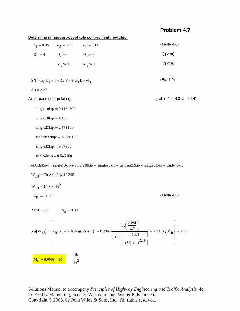
single10kip 0.1121300⋅:=
single18kip 1 120⋅:=
single23kip 2.578 100⋅:=
tandem32kip 0.8886100⋅:=
single32kip 9.871 30⋅:=
triple40kip 0.546 100⋅:=
TotAxleEqv single10kip single18kip+ single23kip+ tandem32kip+ single32kip+ triple40kip+:=
W18 TotAxleEqv 10⋅ 365⋅:=
W18 3.106 106×=
ZR 1.036−:= (Table 4.5)
ΔPSI 2.2:= So 0.30:=
log W18( ) ZR So⋅ 9.36 log SN 1+( )( )+ 0.20−
logΔPSI2.7
⎛⎜⎝
⎞⎟⎠
0.401094
SN 1+( )5.19⎡⎢⎣
⎤⎥⎦
+
+ 2.32 log MR( )⋅+
⎡⎢⎢⎢⎢⎣
⎤⎥⎥⎥⎥⎦
8.07−
lb
in2MR 9.0098 103×=
Problem 4.7Determine minimum acceptable soil resilient modulus.
a1 0.35:= a2 0.20:= a3 0.11:= (Table 4.6)
D1 4:= D2 6:= D3 7:= (given)
M2 1:= M3 1:= (given)
SN a1 D1⋅ a2 D2⋅ M2⋅+ a3 D3⋅ M3⋅+:= (Eq. 4.9)
SN 3.37=
Axle Loads (interpolating): (Table 4.2, 4.3, and 4.4)
Solutions Manual to accompany Principles of Highway Engineering and Traffic Analysis, 4e, by Fred L. Mannering, Scott S. Washburn, and Walter P. Kilareski. Copyright © 2008, by John Wiley & Sons, Inc. All rights reserved.
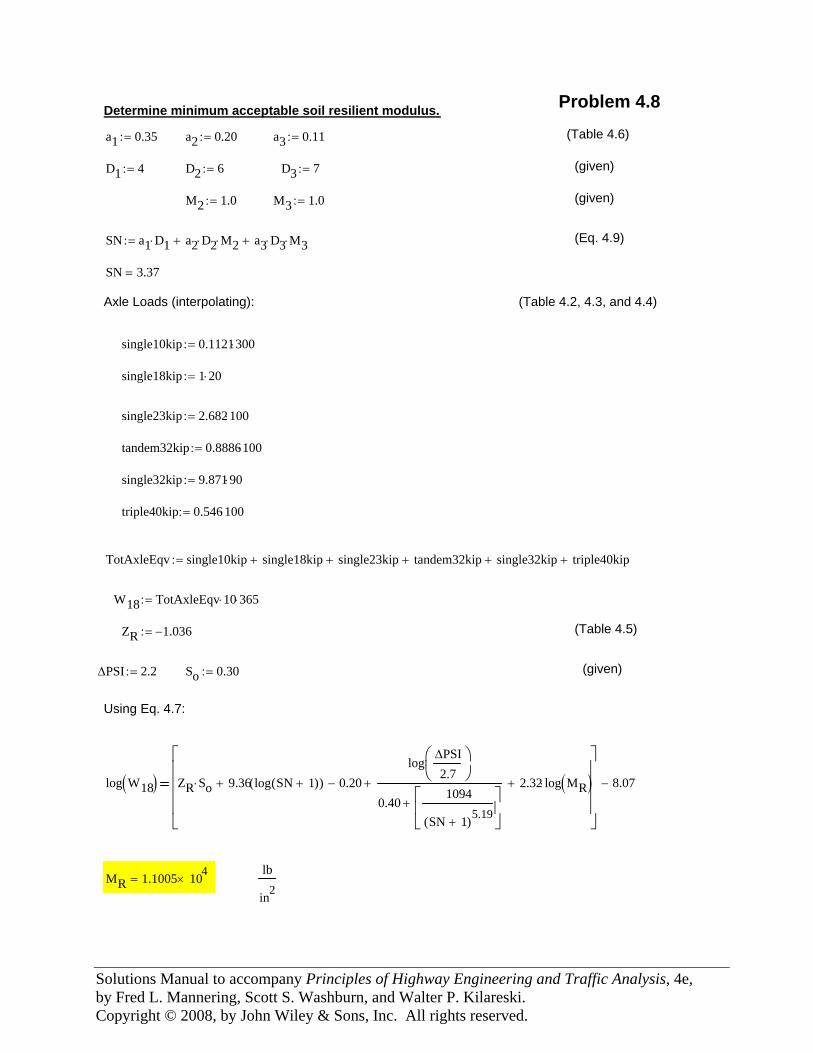
single18kip 1 20⋅:=
single23kip 2.682 100⋅:=
tandem32kip 0.8886100⋅:=
single32kip 9.871 90⋅:=
triple40kip 0.546 100⋅:=
TotAxleEqv single10kip single18kip+ single23kip+ tandem32kip+ single32kip+ triple40kip+:=
W18 TotAxleEqv 10⋅ 365⋅:=
ZR 1.036−:= (Table 4.5)
ΔPSI 2.2:= So 0.30:= (given)
Using Eq. 4.7:
log W18( ) ZR So⋅ 9.36 log SN 1+( )( )+ 0.20−
logΔPSI2.7
⎛⎜⎝
⎞⎟⎠
0.401094
SN 1+( )5.19⎡⎢⎣
⎤⎥⎦
+
+ 2.32 log MR( )⋅+
⎡⎢⎢⎢⎢⎣
⎤⎥⎥⎥⎥⎦
8.07−
MR 1.1005 104×=
lb
in2
Problem 4.8Determine minimum acceptable soil resilient modulus.
a1 0.35:= a2 0.20:= a3 0.11:= (Table 4.6)
D1 4:= D2 6:= D3 7:= (given)
M2 1.0:= M3 1.0:= (given)
SN a1 D1⋅ a2 D2⋅ M2⋅+ a3 D3⋅ M3⋅+:= (Eq. 4.9)
SN 3.37=
Axle Loads (interpolating): (Table 4.2, 4.3, and 4.4)
single10kip 0.1121300⋅:=
Solutions Manual to accompany Principles of Highway Engineering and Traffic Analysis, 4e, by Fred L. Mannering, Scott S. Washburn, and Walter P. Kilareski. Copyright © 2008, by John Wiley & Sons, Inc. All rights reserved.
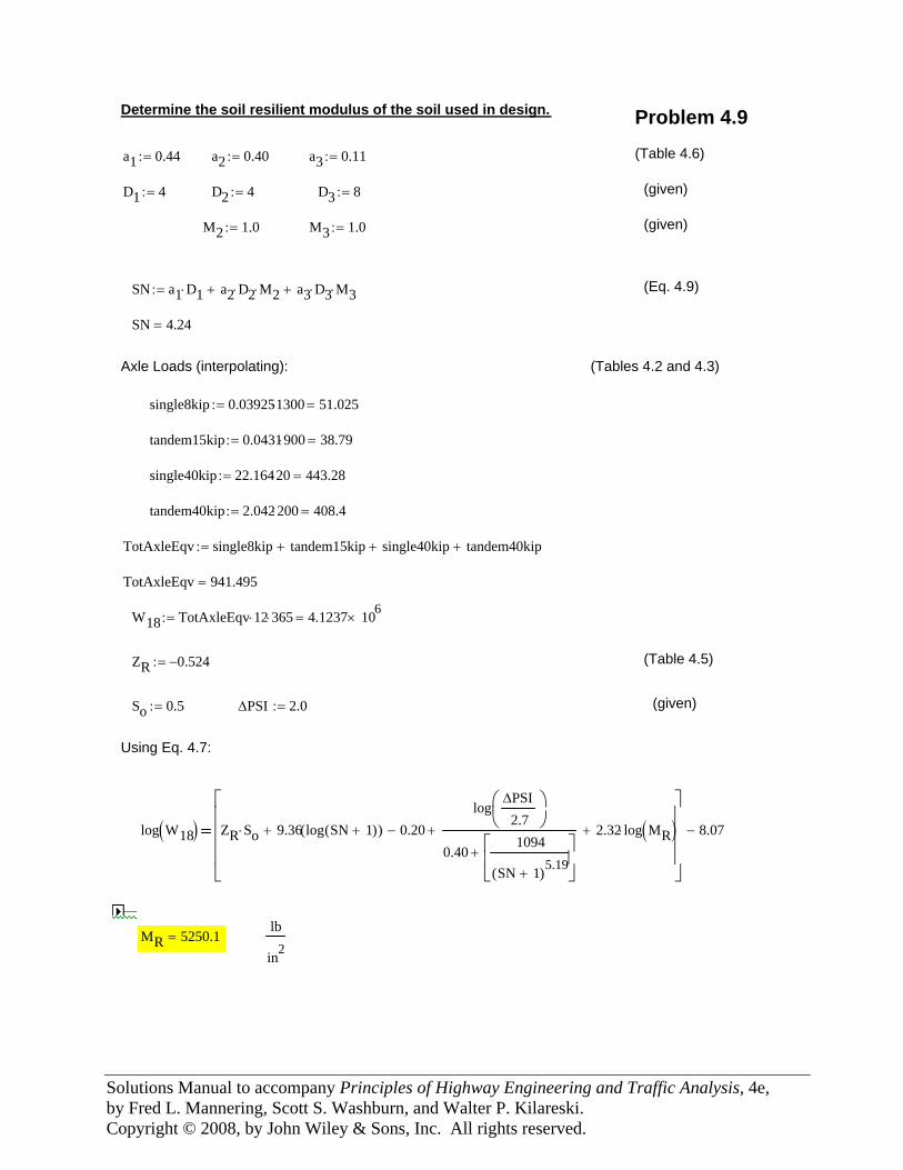
Determine the soil resilient modulus of the soil used in design. Problem 4.9
a1 0.44:= a2 0.40:= a3 0.11:= (Table 4.6)
D1 4:= D2 4:= D3 8:= (given)
M2 1.0:= M3 1.0:= (given)
SN a1 D1⋅ a2 D2⋅ M2⋅+ a3 D3⋅ M3⋅+:= (Eq. 4.9)
SN 4.24=
Axle Loads (interpolating): (Tables 4.2 and 4.3)
single8kip 0.039251300⋅ 51.025=:=
tandem15kip 0.0431900⋅ 38.79=:=
single40kip 22.16420⋅ 443.28=:=
tandem40kip 2.042 200⋅ 408.4=:=
TotAxleEqv single8kip tandem15kip+ single40kip+ tandem40kip+:=
TotAxleEqv 941.495=
W18 TotAxleEqv 12⋅ 365⋅ 4.1237 106×=:=
ZR 0.524−:= (Table 4.5)
So 0.5:= ΔPSI 2.0:= (given)
Using Eq. 4.7:
log W18( ) ZR So⋅ 9.36 log SN 1+( )( )+ 0.20−
logΔPSI
2.7⎛⎜⎝
⎞⎟⎠
0.401094
SN 1+( )5.19⎡⎢⎣
⎤⎥⎦
+
+ 2.32 log MR( )⋅+
⎡⎢⎢⎢⎢⎣
⎤⎥⎥⎥⎥⎦
8.07−
MR 5250.1=lb
in2
Solutions Manual to accompany Principles of Highway Engineering and Traffic Analysis, 4e, by Fred L. Mannering, Scott S. Washburn, and Walter P. Kilareski. Copyright © 2008, by John Wiley & Sons, Inc. All rights reserved.
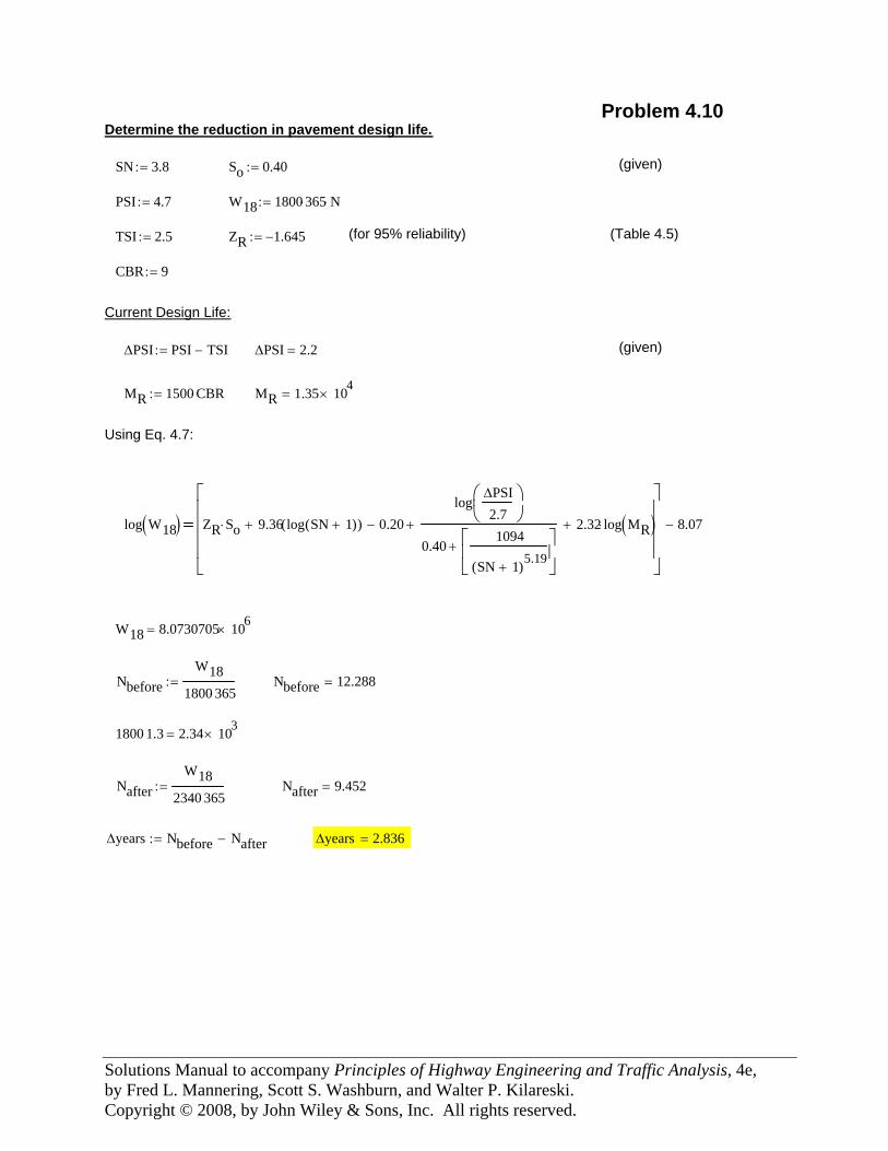
Δyears 2.836=Δyears Nbefore Nafter−:=
Nafter 9.452=NafterW18
2340 365⋅:=
1800 1.3⋅ 2.34 103×=
Nbefore 12.288=NbeforeW18
1800 365⋅:=
W18 8.0730705 106×=
log W18( ) ZR So⋅ 9.36 log SN 1+( )( )+ 0.20−
logΔPSI2.7
⎛⎜⎝
⎞⎟⎠
0.401094
SN 1+( )5.19⎡⎢⎣
⎤⎥⎦
+
+ 2.32 log MR( )⋅+
⎡⎢⎢⎢⎢⎣
⎤⎥⎥⎥⎥⎦
8.07−
Using Eq. 4.7:
MR 1.35 104×=MR 1500 CBR⋅:=
(given)ΔPSI 2.2=ΔPSI PSI TSI−:=
Current Design Life:
CBR 9:=
(Table 4.5)(for 95% reliability)ZR 1.645−:=TSI 2.5:=
W18 1800 365⋅ N⋅:=PSI 4.7:=
(given)So 0.40:=SN 3.8:=
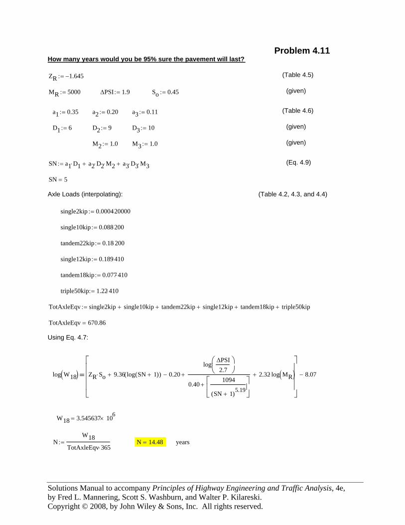
Determine the reduction in pavement design life.Problem 4.10
Solutions Manual to accompany Principles of Highway Engineering and Traffic Analysis, 4e, by Fred L. Mannering, Scott S. Washburn, and Walter P. Kilareski. Copyright © 2008, by John Wiley & Sons, Inc. All rights reserved.
(Eq. 4.9)
SN 5=
Axle Loads (interpolating): (Table 4.2, 4.3, and 4.4)
single2kip 0.000420000⋅:=
single10kip 0.088 200⋅:=
tandem22kip 0.18 200⋅:=
single12kip 0.189 410⋅:=
tandem18kip 0.077 410⋅:=
triple50kip 1.22 410⋅:=
TotAxleEqv single2kip single10kip+ tandem22kip+ single12kip+ tandem18kip+ triple50kip+:=
TotAxleEqv 670.86=
Using Eq. 4.7:
log W18( ) ZR So⋅ 9.36 log SN 1+( )( )+ 0.20−
logΔPSI2.7
⎛⎜⎝
⎞⎟⎠
0.401094
SN 1+( )5.19⎡⎢⎣
⎤⎥⎦
+
+ 2.32 log MR( )⋅+
⎡⎢⎢⎢⎢⎣
⎤⎥⎥⎥⎥⎦
8.07−
W18 3.545637 106×=
NW18
TotAxleEqv 365⋅:= N 14.48= years
Problem 4.11How many years would you be 95% sure the pavement will last?
ZR 1.645−:= (Table 4.5)
MR 5000:= ΔPSI 1.9:= So 0.45:= (given)
a1 0.35:= a2 0.20:= a3 0.11:= (Table 4.6)
D1 6:= D2 9:= D3 10:= (given)
M2 1.0:= M3 1.0:= (given)
SN a1 D1⋅ a2 D2⋅ M2⋅+ a3 D3⋅ M3⋅+:=
Solutions Manual to accompany Principles of Highway Engineering and Traffic Analysis, 4e, by Fred L. Mannering, Scott S. Washburn, and Walter P. Kilareski. Copyright © 2008, by John Wiley & Sons, Inc. All rights reserved.
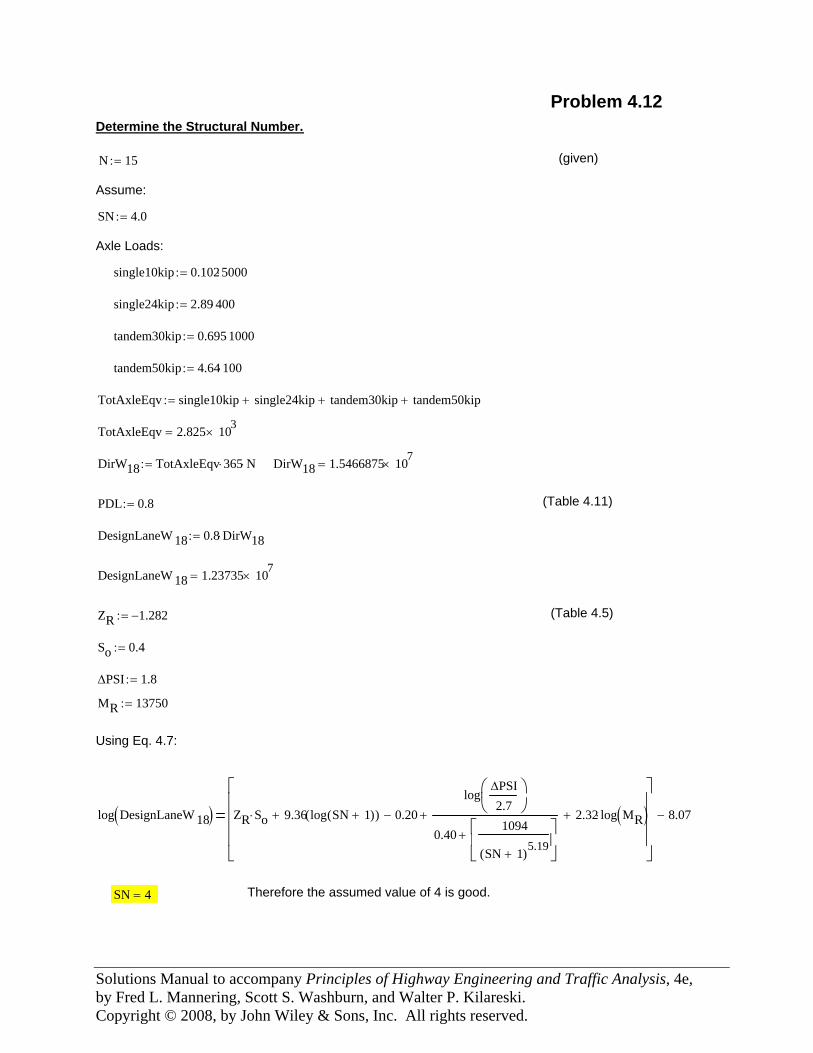
Therefore the assumed value of 4 is good.SN 4=
log DesignLaneW 18( ) ZR So⋅ 9.36 log SN 1+( )( )+ 0.20−
logΔPSI2.7
⎛⎜⎝
⎞⎟⎠
0.401094
SN 1+( )5.19⎡⎢⎣
⎤⎥⎦
+
+ 2.32 log MR( )⋅+
⎡⎢⎢⎢⎢⎣
⎤⎥⎥⎥⎥⎦
8.07−
Using Eq. 4.7:
MR 13750:=
ΔPSI 1.8:=
So 0.4:=
(Table 4.5)ZR 1.282−:=
DesignLaneW 18 1.23735 107×=
DesignLaneW 18 0.8 DirW18⋅:=
(Table 4.11)PDL 0.8:=
DirW18 1.5466875 107×=DirW18 TotAxleEqv 365⋅ N⋅:=
TotAxleEqv 2.825 103×=
TotAxleEqv single10kip single24kip+ tandem30kip+ tandem50kip+:=
tandem50kip 4.64 100⋅:=
tandem30kip 0.695 1000⋅:=
single24kip 2.89 400⋅:=
single10kip 0.102 5000⋅:=
Axle Loads:
SN 4.0:=
Assume:
(given)N 15:=
Determine the Structural Number.
Problem 4.12
Solutions Manual to accompany Principles of Highway Engineering and Traffic Analysis, 4e, by Fred L. Mannering, Scott S. Washburn, and Walter P. Kilareski. Copyright © 2008, by John Wiley & Sons, Inc. All rights reserved.
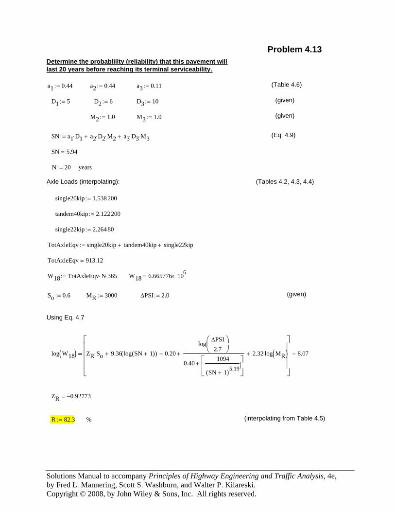
single20kip 1.538 200⋅:=
tandem40kip 2.122 200⋅:=
single22kip 2.264 80⋅:=
TotAxleEqv single20kip tandem40kip+ single22kip+:=
TotAxleEqv 913.12=
W18 TotAxleEqv N⋅ 365⋅:= W18 6.665776 106×=
So 0.6:= MR 3000:= ΔPSI 2.0:= (given)
Using Eq. 4.7
log W18( ) ZR So⋅ 9.36 log SN 1+( )( )+ 0.20−
logΔPSI2.7
⎛⎜⎝
⎞⎟⎠
0.401094
SN 1+( )5.19⎡⎢⎣
⎤⎥⎦
+
+ 2.32 log MR( )⋅+
⎡⎢⎢⎢⎢⎣
⎤⎥⎥⎥⎥⎦
8.07−
ZR 0.92773−=
R 82.3:= % (interpolating from Table 4.5)
Problem 4.13Determine the probablility (reliability) that this pavement willlast 20 years before reaching its terminal serviceability.
a1 0.44:= a2 0.44:= a3 0.11:= (Table 4.6)
D1 5:= D2 6:= D3 10:= (given)
M2 1.0:= M3 1.0:= (given)
SN a1 D1⋅ a2 D2⋅ M2⋅+ a3 D3⋅ M3⋅+:= (Eq. 4.9)
SN 5.94=
N 20:= years
Axle Loads (interpolating): (Tables 4.2, 4.3, 4.4)
Solutions Manual to accompany Principles of Highway Engineering and Traffic Analysis, 4e, by Fred L. Mannering, Scott S. Washburn, and Walter P. Kilareski. Copyright © 2008, by John Wiley & Sons, Inc. All rights reserved.
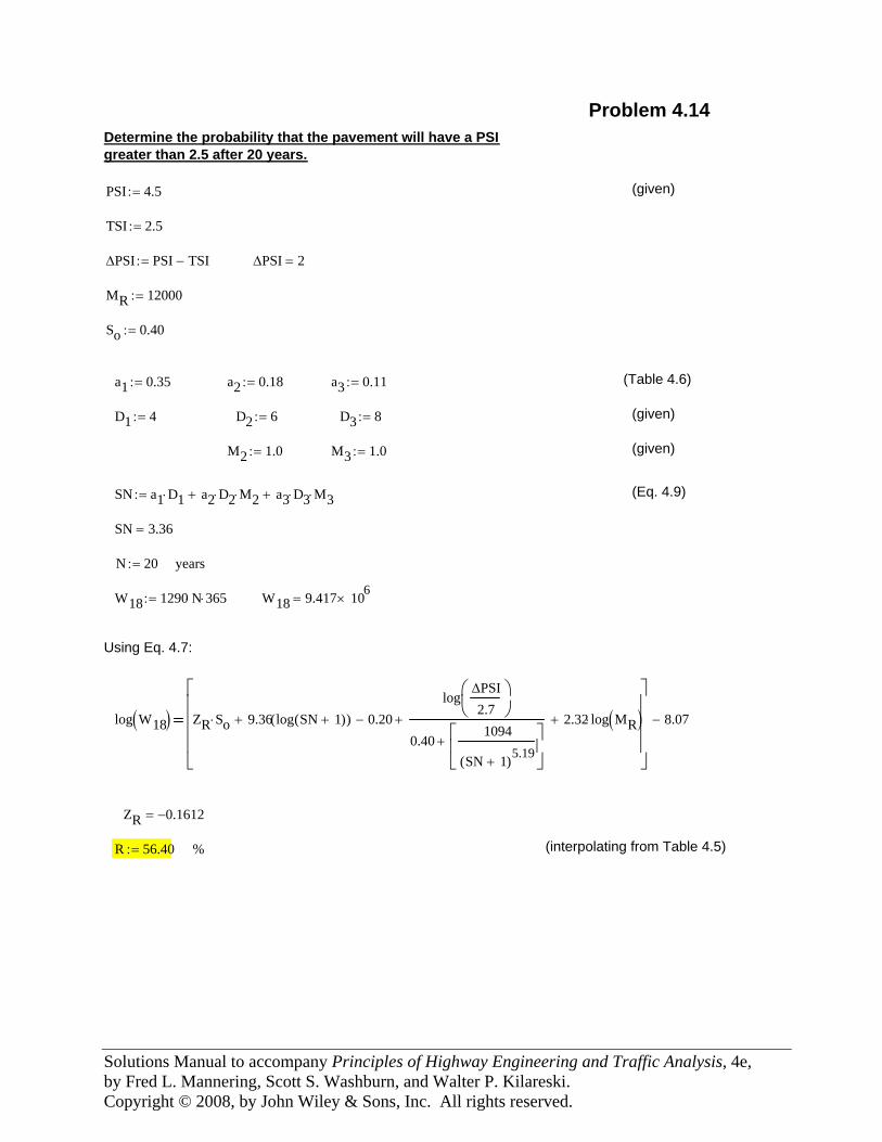
M3 1.0:= (given)
SN a1 D1⋅ a2 D2⋅ M2⋅+ a3 D3⋅ M3⋅+:= (Eq. 4.9)
SN 3.36=
N 20:= years
W18 1290 N⋅ 365⋅:= W18 9.417 106×=
Using Eq. 4.7:
log W18( ) ZR So⋅ 9.36 log SN 1+( )( )+ 0.20−
logΔPSI2.7
⎛⎜⎝
⎞⎟⎠
0.401094
SN 1+( )5.19⎡⎢⎣
⎤⎥⎦
+
+ 2.32 log MR( )⋅+
⎡⎢⎢⎢⎢⎣
⎤⎥⎥⎥⎥⎦
8.07−
ZR 0.1612−=
R 56.40:= % (interpolating from Table 4.5)
Problem 4.14Determine the probability that the pavement will have a PSIgreater than 2.5 after 20 years.
PSI 4.5:= (given)
TSI 2.5:=
ΔPSI PSI TSI−:= ΔPSI 2=
MR 12000:=
So 0.40:=
a1 0.35:= a2 0.18:= a3 0.11:= (Table 4.6)
D1 4:= D2 6:= D3 8:= (given)
M2 1.0:=
Solutions Manual to accompany Principles of Highway Engineering and Traffic Analysis, 4e, by Fred L. Mannering, Scott S. Washburn, and Walter P. Kilareski. Copyright © 2008, by John Wiley & Sons, Inc. All rights reserved.
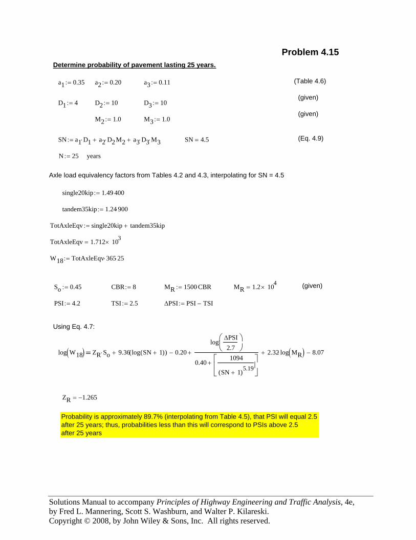
single20kip 1.49 400⋅:=
tandem35kip 1.24 900⋅:=
TotAxleEqv single20kip tandem35kip+:=
TotAxleEqv 1.712 103×=
W18 TotAxleEqv 365⋅ 25⋅:=
So 0.45:= CBR 8:= MR 1500 CBR⋅:= MR 1.2 104×= (given)
PSI 4.2:= TSI 2.5:= ΔPSI PSI TSI−:=
Using Eq. 4.7:
log W18( ) ZR So⋅ 9.36 log SN 1+( )( )+ 0.20−
logΔPSI2.7
⎛⎜⎝
⎞⎟⎠
0.401094
SN 1+( )5.19⎡⎢⎣
⎤⎥⎦
+
+ 2.32 log MR( )⋅+ 8.07−
ZR 1.265−=
Probability is approximately 89.7% (interpolating from Table 4.5), that PSI will equal 2.5after 25 years; thus, probabilities less than this will correspond to PSIs above 2.5after 25 years
Problem 4.15Determine probability of pavement lasting 25 years.
a1 0.35:= a2 0.20:= a3 0.11:= (Table 4.6)
(given)D1 4:= D2 10:= D3 10:=
(given)M2 1.0:= M3 1.0:=
SN a1 D1⋅ a2 D2⋅ M2+ a3 D3⋅ M3⋅+:= SN 4.5= (Eq. 4.9)
N 25:= years
Axle load equivalency factors from Tables 4.2 and 4.3, interpolating for SN = 4.5
Solutions Manual to accompany Principles of Highway Engineering and Traffic Analysis, 4e, by Fred L. Mannering, Scott S. Washburn, and Walter P. Kilareski. Copyright © 2008, by John Wiley & Sons, Inc. All rights reserved.
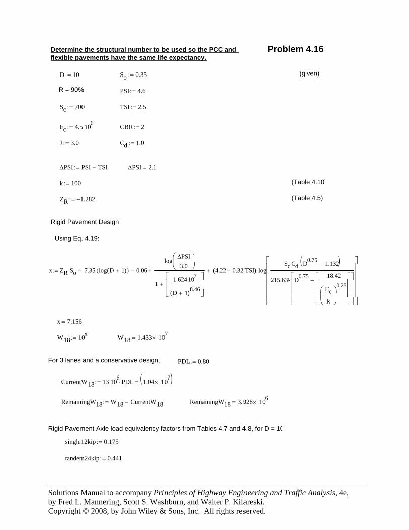
Using Eq. 4.19:
Rigid Pavement Design
(Table 4.5)ZR 1.282−:=
(Table 4.10)k 100:=
ΔPSI 2.1=ΔPSI PSI TSI−:=
Cd 1.0:=J 3.0:=
CBR 2:=Ec 4.5 106⋅:=
TSI 2.5:=Sc 700:=
PSI 4.6:=R = 90%
(given)So 0.35:=D 10:=
Problem 4.16Determine the structural number to be used so the PCC and flexible pavements have the same life expectancy.
x ZR So⋅ 7.35 log D 1+( )( )⋅+ 0.06−
logΔPSI3.0
⎛⎜⎝
⎞⎟⎠
11.624 107
⋅
D 1+( )8.46
⎡⎢⎢⎣
⎤⎥⎥⎦
+
+ 4.22 0.32 TSI⋅−( ) logSc Cd D0.75 1.132−( )⋅
215.63J D0.75 18.42
Eck
⎛⎜⎝
⎞⎟⎠
0.25⎡⎢⎢⎢⎣
⎤⎥⎥⎥⎦
−⎡⎢⎢⎢⎣
⎤⎥⎥⎥⎦
⋅
⎡⎢⎢⎢⎢⎢⎣
⎤⎥⎥⎥⎥⎥⎦
⋅+:=
x 7.156=
W18 10x:= W18 1.433 107
×=
For 3 lanes and a conservative design, PDL 0.80:=
CurrentW18 13 106⋅ PDL⋅:= 1.04 107
×( )=
RemainingW18 W18 CurrentW18−:= RemainingW18 3.928 106×=
Rigid Pavement Axle load equivalency factors from Tables 4.7 and 4.8, for D = 10
single12kip 0.175:=
tandem24kip 0.441:=
Solutions Manual to accompany Principles of Highway Engineering and Traffic Analysis, 4e, by Fred L. Mannering, Scott S. Washburn, and Walter P. Kilareski. Copyright © 2008, by John Wiley & Sons, Inc. All rights reserved.
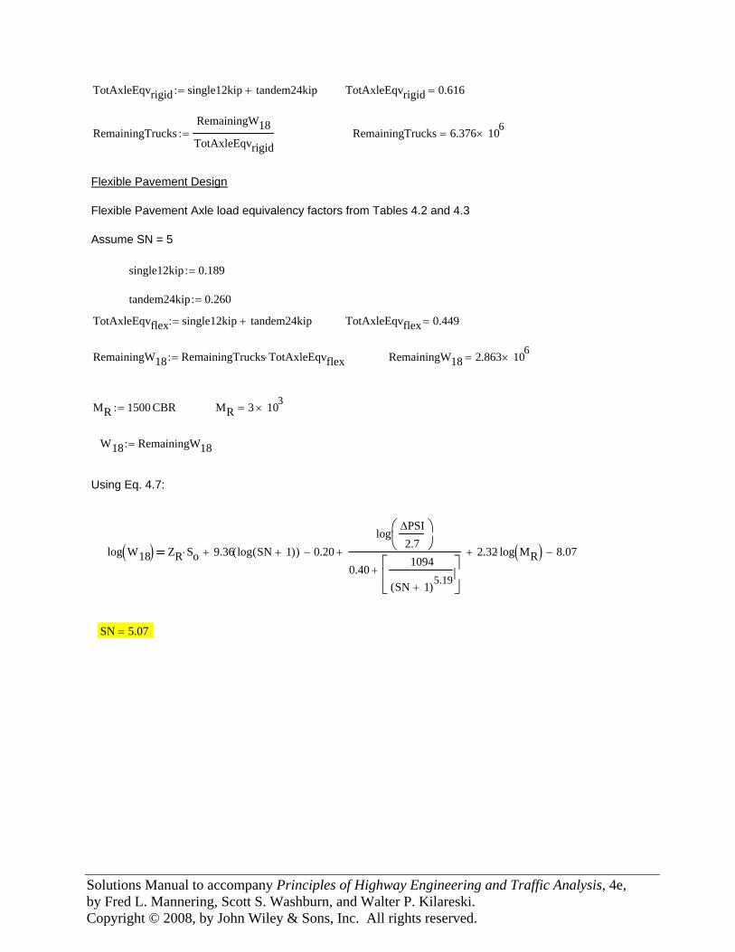
SN 5.07=
log W18( ) ZR So⋅ 9.36 log SN 1+( )( )+ 0.20−
logΔPSI2.7
⎛⎜⎝
⎞⎟⎠
0.401094
SN 1+( )5.19⎡⎢⎣
⎤⎥⎦
+
+ 2.32 log MR( )⋅+ 8.07−
Using Eq. 4.7:
W18 RemainingW18:=
MR 3 103×=MR 1500 CBR⋅:=
RemainingW18 2.863 106×=RemainingW18 RemainingTrucks TotAxleEqvflex⋅:=
TotAxleEqvflex 0.449=TotAxleEqvflex single12kip tandem24kip+:=
tandem24kip 0.260:=
single12kip 0.189:=
Assume SN = 5
Flexible Pavement Axle load equivalency factors from Tables 4.2 and 4.3
Flexible Pavement Design
RemainingTrucks 6.376 106×=RemainingTrucks
RemainingW18TotAxleEqvrigid
:=
TotAxleEqvrigid 0.616=TotAxleEqvrigid single12kip tandem24kip+:=
Solutions Manual to accompany Principles of Highway Engineering and Traffic Analysis, 4e, by Fred L. Mannering, Scott S. Washburn, and Walter P. Kilareski. Copyright © 2008, by John Wiley & Sons, Inc. All rights reserved.
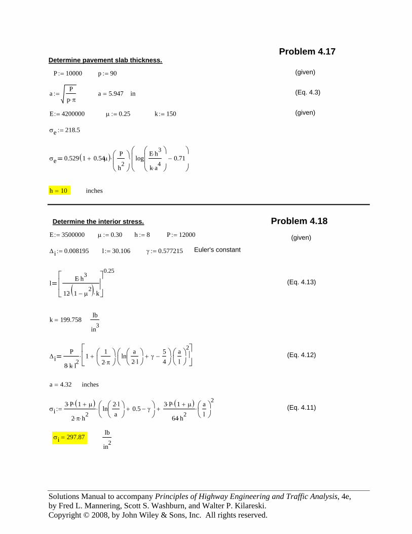
inchesh 10=
σe 0.529 1 0.54μ+( )⋅P
h2⎛⎜⎝
⎞⎟⎠
⋅ logE h3⋅
k a4⋅
⎛⎜⎜⎝
⎞⎟⎟⎠
0.71−⎛⎜⎜⎝
⎞⎟⎟⎠
⋅
σe 218.5:=
(given)k 150:=μ 0.25:=E 4200000:=
(Eq. 4.3)ina 5.947=aP
p π⋅:=
(given)p 90:=P 10000:=
Determine pavement slab thickness.Problem 4.17
lb
in2σi 297.87=
(Eq. 4.11)σi3 P⋅ 1 μ+( )⋅
2 π⋅ h2⋅
ln2 l⋅a
⎛⎜⎝
⎞⎟⎠
0.5+ γ−⎛⎜⎝
⎞⎟⎠
⋅3 P⋅ 1 μ+( )⋅
64 h2⋅
al
⎛⎜⎝
⎞⎟⎠
2⋅+:=
inchesa 4.32=
(Eq. 4.12)ΔiP
8 k⋅ l2⋅1
12 π⋅
⎛⎜⎝
⎞⎟⎠
lna2 l⋅
⎛⎜⎝
⎞⎟⎠
γ+54
−⎛⎜⎝
⎞⎟⎠
⋅al
⎛⎜⎝
⎞⎟⎠
2⋅+
⎡⎢⎣
⎤⎥⎦
⋅
lb
in3k 199.758=
(Eq. 4.13)lE h3⋅
12 1 μ2
−( )⋅ k⋅
⎡⎢⎢⎣
⎤⎥⎥⎦
0.25
Euler's constantγ 0.577215:=l 30.106:=Δi 0.008195:=
(given) P 12000:=h 8:=μ 0.30:=E 3500000:=
Problem 4.18Determine the interior stress.
Solutions Manual to accompany Principles of Highway Engineering and Traffic Analysis, 4e, by Fred L. Mannering, Scott S. Washburn, and Walter P. Kilareski. Copyright © 2008, by John Wiley & Sons, Inc. All rights reserved.
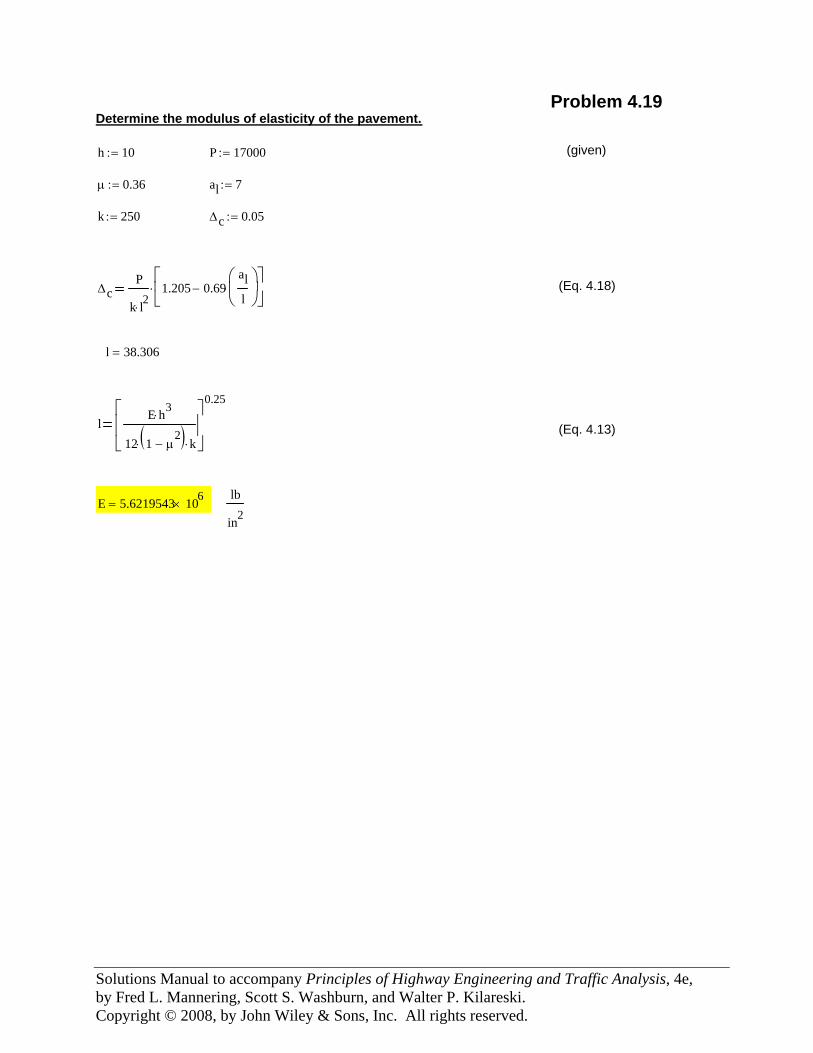
lb
in2E 5.6219543 106
×=
(Eq. 4.13)lE h3⋅
12 1 μ2
−( )⋅ k⋅
⎡⎢⎢⎣
⎤⎥⎥⎦
0.25
l 38.306=
(Eq. 4.18)ΔcP
k l2⋅1.205 0.69
all
⎛⎜⎝
⎞⎟⎠
⋅−⎡⎢⎣
⎤⎥⎦
⋅
Δc 0.05:=k 250:=
al 7:=μ 0.36:=
(given)P 17000:=h 10:=
Determine the modulus of elasticity of the pavement.Problem 4.19
Solutions Manual to accompany Principles of Highway Engineering and Traffic Analysis, 4e, by Fred L. Mannering, Scott S. Washburn, and Walter P. Kilareski. Copyright © 2008, by John Wiley & Sons, Inc. All rights reserved.
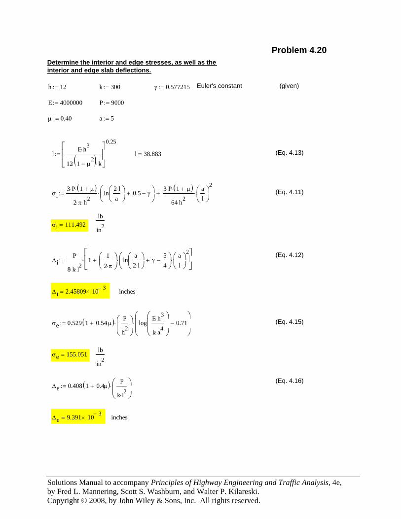
inchesΔe 9.391 10 3−×=
Δe 0.408 1 0.4μ+( )⋅P
k l2⋅
⎛⎜⎝
⎞⎟⎠
⋅:=(Eq. 4.16)
lb
in2σe 155.051=
(Eq. 4.15)σe 0.529 1 0.54μ⋅+( )⋅P
h2⎛⎜⎝
⎞⎟⎠
⋅ logE h3⋅
k a4⋅
⎛⎜⎜⎝
⎞⎟⎟⎠
0.71−⎛⎜⎜⎝
⎞⎟⎟⎠
⋅:=
inchesΔi 2.45809 10 3−×=
ΔiP
8 k⋅ l2⋅1
12 π⋅
⎛⎜⎝
⎞⎟⎠
lna2 l⋅
⎛⎜⎝
⎞⎟⎠
γ+54
−⎛⎜⎝
⎞⎟⎠
⋅al
⎛⎜⎝
⎞⎟⎠
2⋅+
⎡⎢⎣
⎤⎥⎦
⋅:=(Eq. 4.12)
σi 111.492=lb
in2
(Eq. 4.11)σi3 P⋅ 1 μ+( )⋅
2 π⋅ h2⋅
ln2 l⋅a
⎛⎜⎝
⎞⎟⎠
0.5+ γ−⎛⎜⎝
⎞⎟⎠
⋅3 P⋅ 1 μ+( )⋅
64 h2⋅
al
⎛⎜⎝
⎞⎟⎠
2⋅+:=
(Eq. 4.13)l 38.883=lE h3⋅
12 1 μ2
−( )⋅ k⋅
⎡⎢⎢⎣
⎤⎥⎥⎦
0.25
:=
a 5:=μ 0.40:=
P 9000:=E 4000000:=
(given) Euler's constantγ 0.577215:=k 300:=h 12:=
Determine the interior and edge stresses, as well as theinterior and edge slab deflections.
Problem 4.20
Solutions Manual to accompany Principles of Highway Engineering and Traffic Analysis, 4e, by Fred L. Mannering, Scott S. Washburn, and Walter P. Kilareski. Copyright © 2008, by John Wiley & Sons, Inc. All rights reserved.
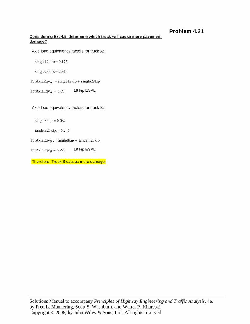
Problem 4.21Considering Ex. 4.5, determine which truck will cause more pavementdamage?
Axle load equivalency factors for truck A:
single12kip 0.175:=
single23kip 2.915:=
TotAxleEqvA single12kip single23kip+:=
TotAxleEqvA 3.09= 18 kip ESAL
Axle load equivalency factors for truck B:
single8kip 0.032:=
tandem23kip 5.245:=
TotAxleEqvB single8kip tandem23kip+:=
TotAxleEqvB 5.277= 18 kip ESAL
Therefore, Truck B causes more damage.
Solutions Manual to accompany Principles of Highway Engineering and Traffic Analysis, 4e, by Fred L. Mannering, Scott S. Washburn, and Walter P. Kilareski. Copyright © 2008, by John Wiley & Sons, Inc. All rights reserved.
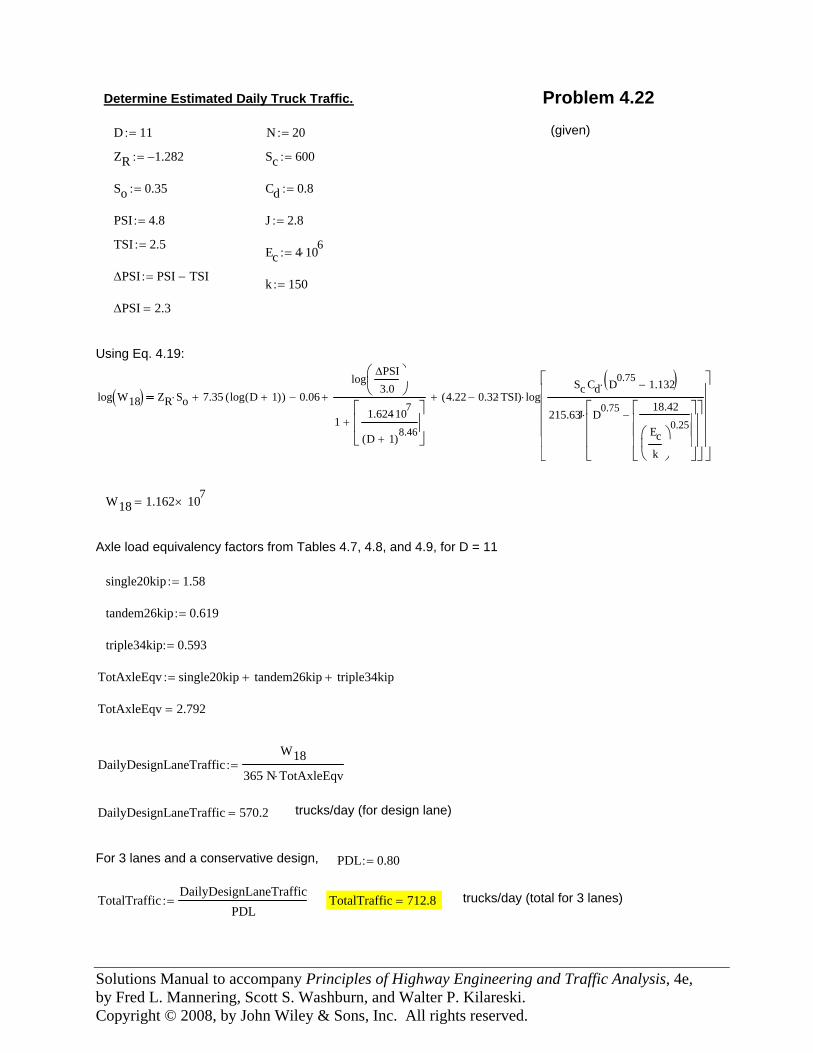
Using Eq. 4.19:
ΔPSI 2.3=
k 150:=ΔPSI PSI TSI−:=
Ec 4 106⋅:=
TSI 2.5:=
J 2.8:=PSI 4.8:=
Cd 0.8:=So 0.35:=
Sc 600:=ZR 1.282−:=
(given) N 20:=D 11:=
Problem 4.22Determine Estimated Daily Truck Traffic.
log W18( ) ZR So⋅ 7.35 log D 1+( )( )⋅+ 0.06−
logΔPSI3.0
⎛⎜⎝
⎞⎟⎠
11.624 107
⋅
D 1+( )8.46
⎡⎢⎢⎣
⎤⎥⎥⎦
+
+ 4.22 0.32 TSI⋅−( ) logSc Cd D0.75 1.132−( )⋅
215.63J D0.75 18.42
Eck
⎛⎜⎝
⎞⎟⎠
0.25⎡⎢⎢⎢⎣
⎤⎥⎥⎥⎦
−⎡⎢⎢⎢⎣
⎤⎥⎥⎥⎦
⋅
⎡⎢⎢⎢⎢⎢⎣
⎤⎥⎥⎥⎥⎥⎦
⋅+
W18 1.162 107×=
Axle load equivalency factors from Tables 4.7, 4.8, and 4.9, for D = 11
single20kip 1.58:=
tandem26kip 0.619:=
triple34kip 0.593:=
TotAxleEqv single20kip tandem26kip+ triple34kip+:=
TotAxleEqv 2.792=
DailyDesignLaneTrafficW18
365 N⋅ TotAxleEqv⋅:=
DailyDesignLaneTraffic 570.2= trucks/day (for design lane)
For 3 lanes and a conservative design, PDL 0.80:=
TotalTrafficDailyDesignLaneTraffic
PDL:= TotalTraffic 712.8= trucks/day (total for 3 lanes)
Solutions Manual to accompany Principles of Highway Engineering and Traffic Analysis, 4e, by Fred L. Mannering, Scott S. Washburn, and Walter P. Kilareski. Copyright © 2008, by John Wiley & Sons, Inc. All rights reserved.
Using Eq. 4.19:
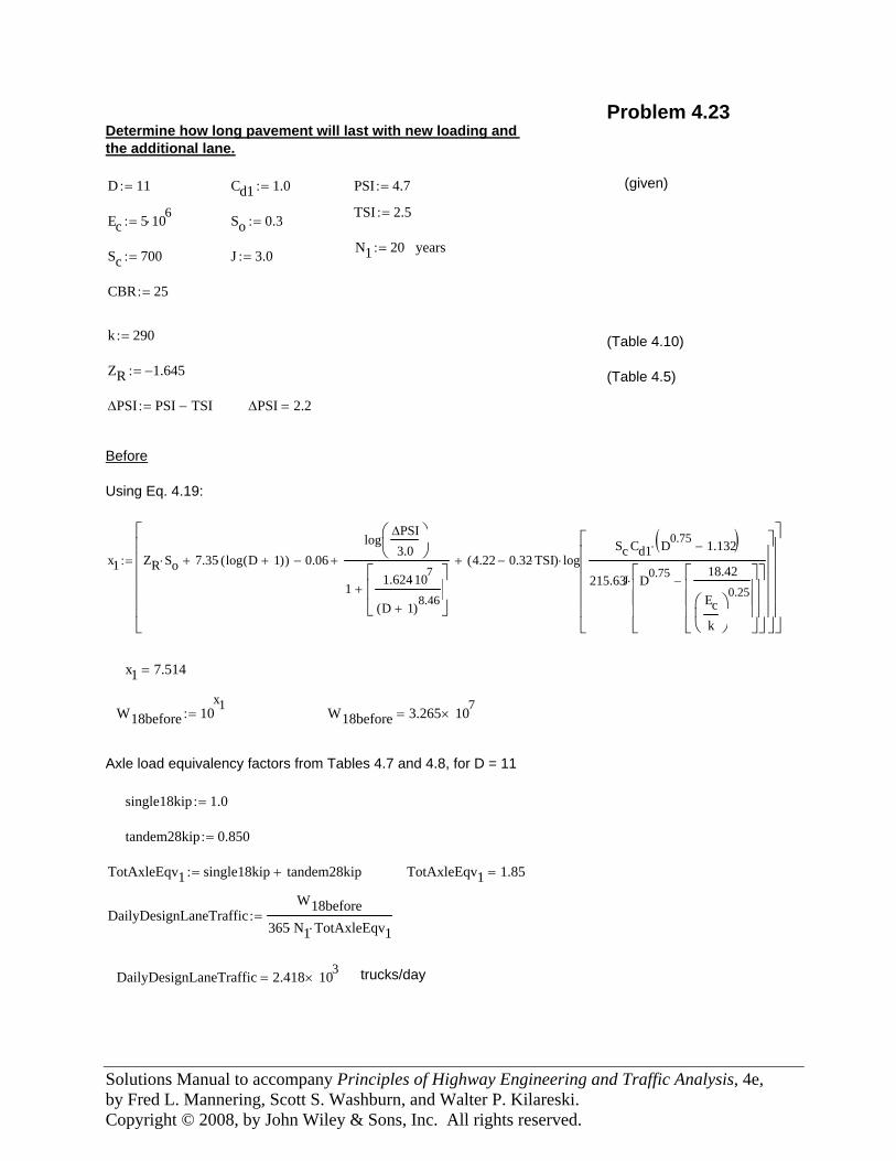
Before
ΔPSI 2.2=ΔPSI PSI TSI−:=
(Table 4.5)ZR 1.645−:=
(Table 4.10)k 290:=
CBR 25:=
J 3.0:=Sc 700:=yearsN1 20:=
So 0.3:=Ec 5 106⋅:=
TSI 2.5:=
(given) PSI 4.7:=Cd1 1.0:=D 11:=
Determine how long pavement will last with new loading andthe additional lane.
Problem 4.23
x1 ZR So⋅ 7.35 log D 1+( )( )⋅+ 0.06−
logΔPSI3.0
⎛⎜⎝
⎞⎟⎠
11.624 107
⋅
D 1+( )8.46
⎡⎢⎢⎣
⎤⎥⎥⎦
+
+ 4.22 0.32 TSI⋅−( ) logSc Cd1 D0.75 1.132−( )⋅
215.63J D0.75 18.42
Eck
⎛⎜⎝
⎞⎟⎠
0.25⎡⎢⎢⎢⎣
⎤⎥⎥⎥⎦
−⎡⎢⎢⎢⎣
⎤⎥⎥⎥⎦
⋅
⎡⎢⎢⎢⎢⎢⎣
⎤⎥⎥⎥⎥⎥⎦
⋅+
⎡⎢⎢⎢⎢⎢⎣
⎤⎥⎥⎥⎥⎥⎦
:=
x1 7.514=
W18before 10x1
:= W18before 3.265 107×=
Axle load equivalency factors from Tables 4.7 and 4.8, for D = 11
single18kip 1.0:=
tandem28kip 0.850:=
TotAxleEqv1 single18kip tandem28kip+:= TotAxleEqv1 1.85=
DailyDesignLaneTrafficW18before
365 N1⋅ TotAxleEqv1⋅:=
DailyDesignLaneTraffic 2.418 103×= trucks/day
Solutions Manual to accompany Principles of Highway Engineering and Traffic Analysis, 4e, by Fred L. Mannering, Scott S. Washburn, and Walter P. Kilareski. Copyright © 2008, by John Wiley & Sons, Inc. All rights reserved.
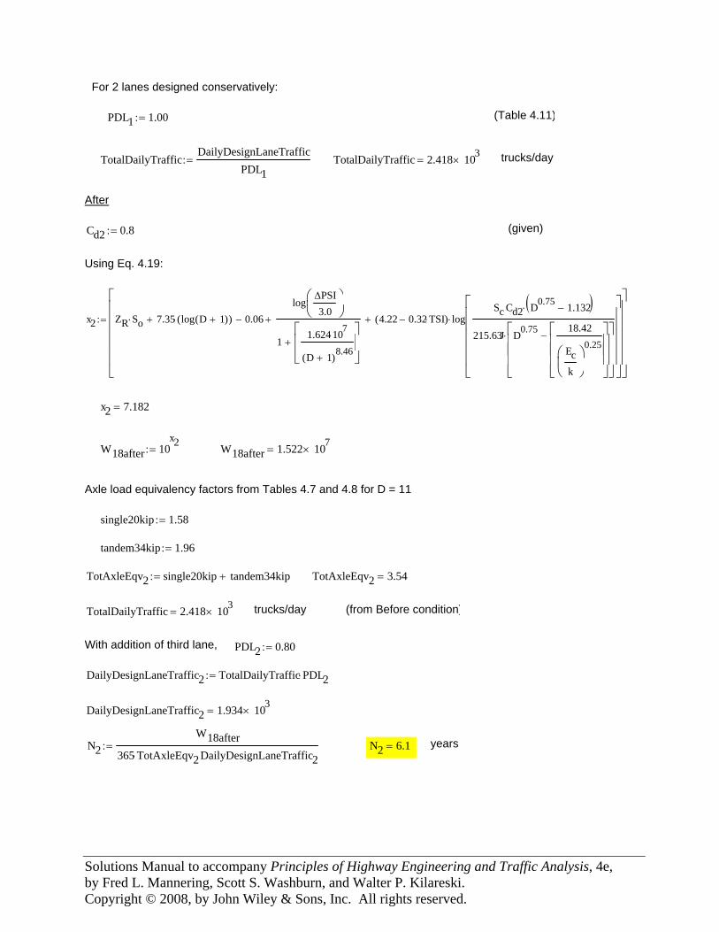
For 2 lanes designed conservatively:
PDL1 1.00:= (Table 4.11)
TotalDailyTrafficDailyDesignLaneTraffic
PDL1:= TotalDailyTraffic 2.418 103
×= trucks/day
After
Cd2 0.8:= (given)
Using Eq. 4.19:
x2 ZR So⋅ 7.35 log D 1+( )( )⋅+ 0.06−
logΔPSI3.0
⎛⎜⎝
⎞⎟⎠
11.624 107
⋅
D 1+( )8.46
⎡⎢⎢⎣
⎤⎥⎥⎦
+
+ 4.22 0.32 TSI⋅−( ) logSc Cd2 D0.75 1.132−( )⋅
215.63J D0.75 18.42
Eck
⎛⎜⎝
⎞⎟⎠
0.25⎡⎢⎢⎢⎣
⎤⎥⎥⎥⎦
−⎡⎢⎢⎢⎣
⎤⎥⎥⎥⎦
⋅
⎡⎢⎢⎢⎢⎢⎣
⎤⎥⎥⎥⎥⎥⎦
⋅+
⎡⎢⎢⎢⎢⎢⎣
⎤⎥⎥⎥⎥⎥⎦
:=
yearsN2 6.1=N2W18after
365 TotAxleEqv2⋅ DailyDesignLaneTraffic2:=
DailyDesignLaneTraffic2 1.934 103×=
DailyDesignLaneTraffic2 TotalDailyTraffic PDL2⋅:=
PDL2 0.80:=With addition of third lane,
(from Before condition)trucks/dayTotalDailyTraffic 2.418 103×=
TotAxleEqv2 3.54=TotAxleEqv2 single20kip tandem34kip+:=
tandem34kip 1.96:=
single20kip 1.58:=
Axle load equivalency factors from Tables 4.7 and 4.8 for D = 11
W18after 1.522 107×=W18after 10
x2:=
x2 7.182=
Solutions Manual to accompany Principles of Highway Engineering and Traffic Analysis, 4e, by Fred L. Mannering, Scott S. Washburn, and Walter P. Kilareski. Copyright © 2008, by John Wiley & Sons, Inc. All rights reserved.
Using Eq. 4.19:
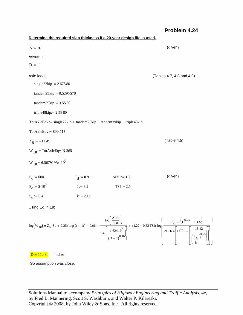
k 200:=So 0.4:=
TSI 2.5:=J 3.2:=Ec 5 106⋅:=
(given) ΔPSI 1.7:=Cd 0.9:=Sc 600:=
W18 6.5679195 106×=
W18 TotAxleEqv N⋅ 365⋅:=
(Table 4.5)ZR 1.645−:=
TotAxleEqv 899.715=
TotAxleEqv single22kip tandem25kip+ tandem39kip+ triple48kip+:=
triple48kip 2.58 80⋅:=
tandem39kip 3.55 50⋅:=
tandem25kip 0.5295570⋅:=
single22kip 2.675 80⋅:=
(Tables 4.7, 4.8 and 4.9)Axle loads:
D 11:=
Assume:
(given) N 20:=
Determine the required slab thickness if a 20-year design life is used.
Problem 4.24
log W18( ) ZR So⋅ 7.35 log D 1+( )( )⋅+ 0.06−
logΔPSI3.0
⎛⎜⎝
⎞⎟⎠
11.624 107⋅
D 1+( )8.46
⎡⎢⎢⎣
⎤⎥⎥⎦
+
+ 4.22 0.32 TSI⋅−( ) logSc Cd D0.75 1.132−( )⋅
215.63J D0.75 18.42
Eck
⎛⎜⎝
⎞⎟⎠
0.25⎡⎢⎢⎢⎣
⎤⎥⎥⎥⎦
−⎡⎢⎢⎢⎣
⎤⎥⎥⎥⎦
⋅
⎡⎢⎢⎢⎢⎢⎣
⎤⎥⎥⎥⎥⎥⎦
⋅+
D 11.43= inches
So assumption was close.
Solutions Manual to accompany Principles of Highway Engineering and Traffic Analysis, 4e, by Fred L. Mannering, Scott S. Washburn, and Walter P. Kilareski. Copyright © 2008, by John Wiley & Sons, Inc. All rights reserved.
Using Eq. 4.19
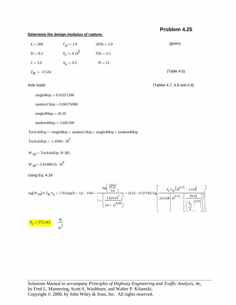
W18 5.9148615 106×=
W18 TotAxleEqv N⋅ 365⋅:=
TotAxleEqv 1.3504 103×=
TotAxleEqv single8kip tandem15kip+ single40kip+ tandem40kip+:=
tandem40kip 3.645 200⋅:=
single40kip 26 20⋅:=
tandem15kip 0.06575900⋅:=
single8kip 0.03251300⋅:=
(Tables 4.7, 4.8 and 4.9)Axle loads:
(Table 4.5)ZR 0.524−:=
N 12:=So 0.5:=J 3.0:=
TSI 2.5:=Ec 4 106⋅:=D 8.5:=
(given) ΔPSI 2.0:=Cd 1.0:=k 300:=
Determine the design modulus of rupture.Problem 4.25
log W18( ) ZR So⋅ 7.35 log D 1+( )( )⋅+ 0.06−
logΔPSI3.0
⎛⎜⎝
⎞⎟⎠
11.624 107⋅
D 1+( )8.46
⎡⎢⎢⎣
⎤⎥⎥⎦
+
+ 4.22 0.32 TSI⋅−( ) logSc Cd D0.75 1.132−( )⋅
215.63J D0.75 18.42
Eck
⎛⎜⎝
⎞⎟⎠
0.25⎡⎢⎢⎢⎣
⎤⎥⎥⎥⎦
−⎡⎢⎢⎢⎣
⎤⎥⎥⎥⎦
⋅
⎡⎢⎢⎢⎢⎢⎣
⎤⎥⎥⎥⎥⎥⎦
⋅+
Sc 575.343=lb
in2
Solutions Manual to accompany Principles of Highway Engineering and Traffic Analysis, 4e, by Fred L. Mannering, Scott S. Washburn, and Walter P. Kilareski. Copyright © 2008, by John Wiley & Sons, Inc. All rights reserved.
Using Eq. 4.19:
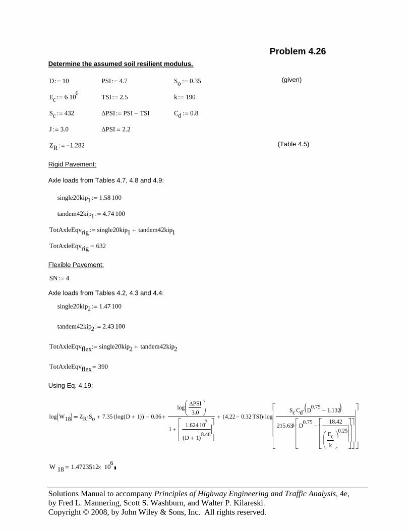
TotAxleEqvflex 390=
TotAxleEqvflex single20kip2 tandem42kip2+:=
tandem42kip2 2.43 100⋅:=
single20kip2 1.47 100⋅:=
Axle loads from Tables 4.2, 4.3 and 4.4:
SN 4:=
Flexible Pavement:
TotAxleEqvrig 632=
TotAxleEqvrig single20kip1 tandem42kip1+:=
tandem42kip1 4.74 100⋅:=
single20kip1 1.58 100⋅:=
Axle loads from Tables 4.7, 4.8 and 4.9:
Rigid Pavement:
(Table 4.5)ZR 1.282−:=
ΔPSI 2.2=J 3.0:=
Cd 0.8:=ΔPSI PSI TSI−:=Sc 432:=
k 190:=TSI 2.5:=Ec 6 106⋅:=
(given) So 0.35:=PSI 4.7:=D 10:=
Determine the assumed soil resilient modulus.
Problem 4.26
log W18( ) ZR So⋅ 7.35 log D 1+( )( )⋅+ 0.06−
logΔPSI3.0
⎛⎜⎝
⎞⎟⎠
11.624 107⋅
D 1+( )8.46
⎡⎢⎢⎣
⎤⎥⎥⎦
+
+ 4.22 0.32 TSI⋅−( ) logSc Cd D0.75 1.132−( )⋅
215.63J D0.75 18.42
Eck
⎛⎜⎝
⎞⎟⎠
0.25⎡⎢⎢⎢⎣
⎤⎥⎥⎥⎦
−⎡⎢⎢⎢⎣
⎤⎥⎥⎥⎦
⋅
⎡⎢⎢⎢⎢⎢⎣
⎤⎥⎥⎥⎥⎥⎦
⋅+
W 18 1.4723512 106
×=
Solutions Manual to accompany Principles of Highway Engineering and Traffic Analysis, 4e, by Fred L. Mannering, Scott S. Washburn, and Walter P. Kilareski. Copyright © 2008, by John Wiley & Sons, Inc. All rights reserved.
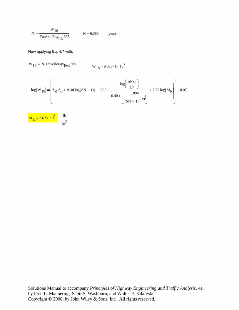
NW18
TotAxleEqvrig 365⋅:= N 6.383= years
Now applying Eq. 4.7 with:
W18 N TotAxleEqvflex⋅ 365⋅:= W18 9.08571 105×=
log W18( ) ZR So⋅ 9.36 log SN 1+( )( )+ 0.20−
logΔPSI2.7
⎛⎜⎝
⎞⎟⎠
0.401094
SN 1+( )5.19⎡⎢⎣
⎤⎥⎦
+
+ 2.32 log MR( )⋅+
⎡⎢⎢⎢⎢⎣
⎤⎥⎥⎥⎥⎦
8.07−
MR 3.67 103×=
lb
in2
Solutions Manual to accompany Principles of Highway Engineering and Traffic Analysis, 4e, by Fred L. Mannering, Scott S. Washburn, and Walter P. Kilareski. Copyright © 2008, by John Wiley & Sons, Inc. All rights reserved.
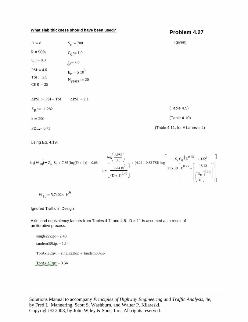
What slab thickness should have been used? Problem 4.27
D 8:= Sc 700:= (given)
R = 90% Cd 1.0:=
So 0.3:= J 3.0:=
PSI 4.6:= Ec 5 106⋅:=
TSI 2.5:= Nyears 20:=CBR 25:=
ΔPSI PSI TSI−:= ΔPSI 2.1=
ZR 1.282−:= (Table 4.5)
k 290:= (Table 4.10)
PDL 0.75:= (Table 4.11, for # Lanes = 4)
Using Eq. 4.19:
log W18( ) ZR So⋅ 7.35 log D 1+( )( )⋅+ 0.06−
logΔPSI3.0
⎛⎜⎝
⎞⎟⎠
11.624 107⋅
D 1+( )8.46
⎡⎢⎢⎣
⎤⎥⎥⎦
+
+ 4.22 0.32 TSI⋅−( ) logSc Cd D0.75 1.132−( )⋅
215.63J D0.75 18.42
Eck
⎛⎜⎝
⎞⎟⎠
0.25⎡⎢⎢⎢⎣
⎤⎥⎥⎥⎦
−⎡⎢⎢⎢⎣
⎤⎥⎥⎥⎦
⋅
⎡⎢⎢⎢⎢⎢⎣
⎤⎥⎥⎥⎥⎥⎦
⋅+
W18 5.7402 106×=
Ignored Traffic in Design
Axle load equivalency factors from Tables 4.7, and 4.8. D = 11 is assumed as a result ofan iterative process.
single22kip 2.40:=
tandem30kip 1.14:=
TotAxleEqv single22kip tandem30kip+:=
TotAxleEqv 3.54:=
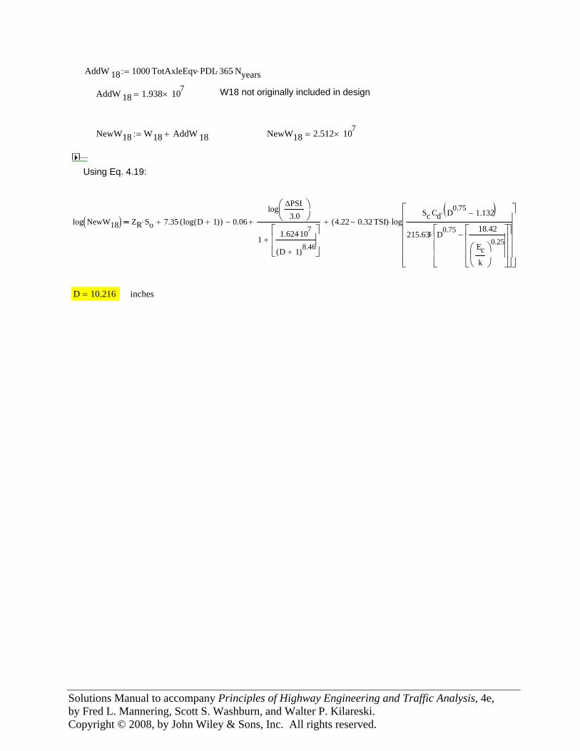
Solutions Manual to accompany Principles of Highway Engineering and Traffic Analysis, 4e, by Fred L. Mannering, Scott S. Washburn, and Walter P. Kilareski. Copyright © 2008, by John Wiley & Sons, Inc. All rights reserved.
AddW 18 1000 TotAxleEqv⋅ PDL⋅ 365⋅ Nyears⋅:=
AddW 18 1.938 107×= W18 not originally included in design
NewW18 W18 AddW 18+:= NewW18 2.512 107×=
Using Eq. 4.19:
log NewW18( ) ZR So⋅ 7.35 log D 1+( )( )⋅+ 0.06−
logΔPSI
3.0⎛⎜⎝
⎞⎟⎠
11.624 107⋅
D 1+( )8.46
⎡⎢⎢⎣
⎤⎥⎥⎦
+
+ 4.22 0.32 TSI⋅−( ) logSc Cd D0.75 1.132−( )⋅
215.63J D0.75 18.42
Eck
⎛⎜⎝
⎞⎟⎠
0.25⎡⎢⎢⎢⎣
⎤⎥⎥⎥⎦
−⎡⎢⎢⎢⎣
⎤⎥⎥⎥⎦
⋅
⎡⎢⎢⎢⎢⎢⎣
⎤⎥⎥⎥⎥⎥⎦
⋅+
D 10.216= inches
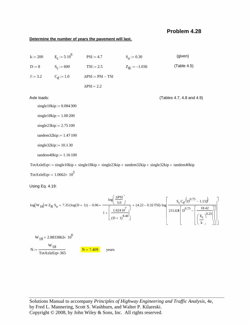
Solutions Manual to accompany Principles of Highway Engineering and Traffic Analysis, 4e, by Fred L. Mannering, Scott S. Washburn, and Walter P. Kilareski. Copyright © 2008, by John Wiley & Sons, Inc. All rights reserved.
Using Eq. 4.19:
TotAxleEqv 1.0662 103×=
TotAxleEqv single10kip single18kip+ single23kip+ tandem32kip+ single32kip+ tandem40kip+:=
tandem40kip 1.16 100⋅:=
single32kip 10.1 30⋅:=
tandem32kip 1.47 100⋅:=
single23kip 2.75 100⋅:=
single18kip 1.00 200⋅:=
single10kip 0.084 300⋅:=
(Tables 4.7, 4.8 and 4.9)Axle loads:
ΔPSI 2.2=
ΔPSI PSI TSI−:=Cd 1.0:=J 3.2:=
(Table 4.5)ZR 1.036−:=TSI 2.5:=Sc 600:=D 8:=
(given) So 0.30:=PSI 4.7:=Ec 5 106⋅:=k 200:=
Determine the number of years the pavement will last.
Problem 4.28
log W18( ) ZR So⋅ 7.35 log D 1+( )( )⋅+ 0.06−
logΔPSI3.0
⎛⎜⎝
⎞⎟⎠
11.624 107⋅
D 1+( )8.46
⎡⎢⎢⎣
⎤⎥⎥⎦
+
+ 4.22 0.32 TSI⋅−( ) logSc Cd D0.75 1.132−( )⋅
215.63J D0.75 18.42
Eck
⎛⎜⎝
⎞⎟⎠
0.25⎡⎢⎢⎢⎣
⎤⎥⎥⎥⎦
−⎡⎢⎢⎢⎣
⎤⎥⎥⎥⎦
⋅
⎡⎢⎢⎢⎢⎢⎣
⎤⎥⎥⎥⎥⎥⎦
⋅+
W18 2.8833862 106×=
NW18
TotAxleEqv 365⋅:= N 7.409= years
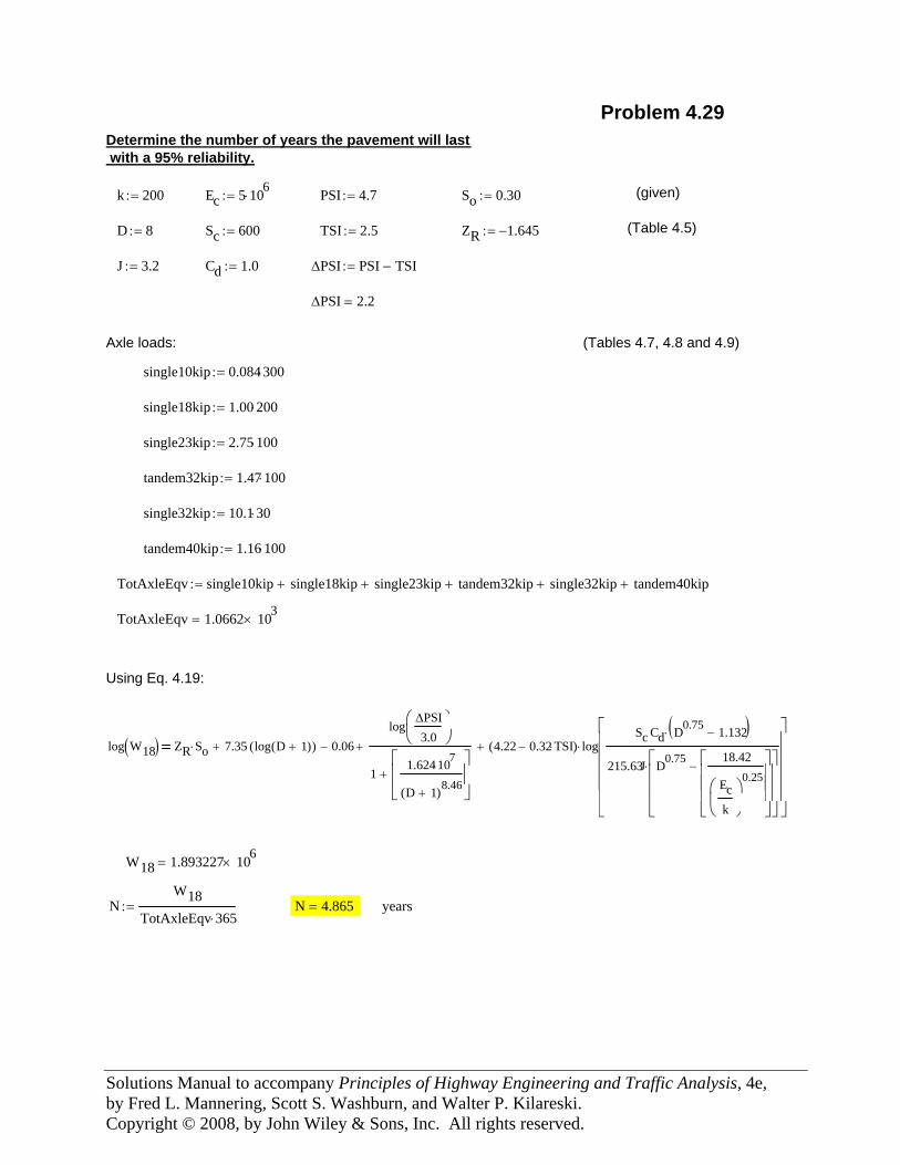
Solutions Manual to accompany Principles of Highway Engineering and Traffic Analysis, 4e, by Fred L. Mannering, Scott S. Washburn, and Walter P. Kilareski. Copyright © 2008, by John Wiley & Sons, Inc. All rights reserved.
Using Eq. 4.19:
TotAxleEqv 1.0662 103×=
TotAxleEqv single10kip single18kip+ single23kip+ tandem32kip+ single32kip+ tandem40kip+:=
tandem40kip 1.16 100⋅:=
single32kip 10.1 30⋅:=
tandem32kip 1.47 100⋅:=
single23kip 2.75 100⋅:=
single18kip 1.00 200⋅:=
single10kip 0.084 300⋅:=
(Tables 4.7, 4.8 and 4.9)Axle loads:
ΔPSI 2.2=
ΔPSI PSI TSI−:=Cd 1.0:=J 3.2:=
(Table 4.5)ZR 1.645−:=TSI 2.5:=Sc 600:=D 8:=
(given) So 0.30:=PSI 4.7:=Ec 5 106⋅:=k 200:=
Determine the number of years the pavement will last with a 95% reliability.
Problem 4.29
log W18( ) ZR So⋅ 7.35 log D 1+( )( )⋅+ 0.06−
logΔPSI3.0
⎛⎜⎝
⎞⎟⎠
11.624 107⋅
D 1+( )8.46
⎡⎢⎢⎣
⎤⎥⎥⎦
+
+ 4.22 0.32 TSI⋅−( ) logSc Cd D0.75 1.132−( )⋅
215.63J D0.75 18.42
Eck
⎛⎜⎝
⎞⎟⎠
0.25⎡⎢⎢⎢⎣
⎤⎥⎥⎥⎦
−⎡⎢⎢⎢⎣
⎤⎥⎥⎥⎦
⋅
⎡⎢⎢⎢⎢⎢⎣
⎤⎥⎥⎥⎥⎥⎦
⋅+
W18 1.893227 106×=
NW18
TotAxleEqv 365⋅:= N 4.865= years
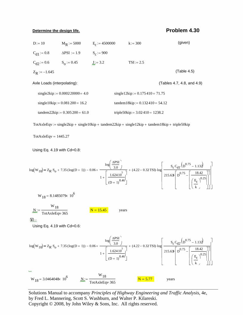
Solutions Manual to accompany Principles of Highway Engineering and Traffic Analysis, 4e, by Fred L. Mannering, Scott S. Washburn, and Walter P. Kilareski. Copyright © 2008, by John Wiley & Sons, Inc. All rights reserved.
Determine the design life. Problem 4.30
D 10:= MR 5000:= Ec 4500000:= k 300:= (given)
Cd1 0.8:= ΔPSI 1.9:= Sc 900:=
Cd2 0.6:= So 0.45:= J 3.2:= TSI 2.5:=
ZR 1.645−:= (Table 4.5)
Axle Loads (interpolating): (Tables 4.7, 4.8, and 4.9)
single2kip 0.000220000⋅ 4.0=:= single12kip 0.175 410⋅ 71.75=:=
single10kip 0.081 200⋅ 16.2=:= tandem18kip 0.132 410⋅ 54.12=:=
tandem22kip 0.305 200⋅ 61.0=:= triple50kip 3.02 410⋅ 1238.2=:=
TotAxleEqv single2kip single10kip+ tandem22kip+ single12kip+ tandem18kip+ triple50kip+:=
TotAxleEqv 1445.27=
Using Eq. 4.19 with Cd=0.8:
log W18( ) ZR So⋅ 7.35 log D 1+( )( )⋅+ 0.06−
logΔPSI3.0
⎛⎜⎝
⎞⎟⎠
11.624 107⋅
D 1+( )8.46
⎡⎢⎢⎣
⎤⎥⎥⎦
+
+ 4.22 0.32 TSI⋅−( ) logSc Cd1 D0.75 1.132−( )⋅
215.63J D0.75 18.42
Eck
⎛⎜⎝
⎞⎟⎠
0.25⎡⎢⎢⎢⎣
⎤⎥⎥⎥⎦
−⎡⎢⎢⎢⎣
⎤⎥⎥⎥⎦
⋅
⎡⎢⎢⎢⎢⎢⎣
⎤⎥⎥⎥⎥⎥⎦
⋅+
W18 8.1485079 106
×=
NW18
TotAxleEqv 365⋅:= N 15.45= years
Using Eq. 4.19 with Cd=0.6:
log W18( ) ZR So⋅ 7.35 log D 1+( )( )⋅+ 0.06−
logΔPSI3.0
⎛⎜⎝
⎞⎟⎠
11.624 107⋅
D 1+( )8.46
⎡⎢⎢⎣
⎤⎥⎥⎦
+
+ 4.22 0.32 TSI⋅−( ) logSc Cd2 D0.75 1.132−( )⋅
215.63J D0.75 18.42
Eck
⎛⎜⎝
⎞⎟⎠
0.25⎡⎢⎢⎢⎣
⎤⎥⎥⎥⎦
−⎡⎢⎢⎢⎣
⎤⎥⎥⎥⎦
⋅
⎡⎢⎢⎢⎢⎢⎣
⎤⎥⎥⎥⎥⎥⎦
⋅+
W18 3.0464048 106×= N
W18TotAxleEqv 365⋅
:= N 5.77= years
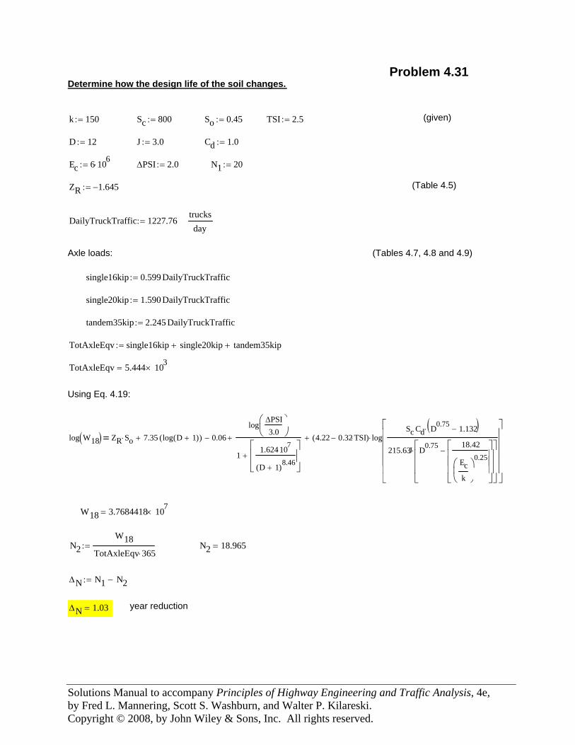
Solutions Manual to accompany Principles of Highway Engineering and Traffic Analysis, 4e, by Fred L. Mannering, Scott S. Washburn, and Walter P. Kilareski. Copyright © 2008, by John Wiley & Sons, Inc. All rights reserved.
Using Eq. 4.19:
TotAxleEqv 5.444 103×=
TotAxleEqv single16kip single20kip+ tandem35kip+:=
tandem35kip 2.245 DailyTruckTraffic⋅:=
single20kip 1.590 DailyTruckTraffic⋅:=
single16kip 0.599 DailyTruckTraffic⋅:=
(Tables 4.7, 4.8 and 4.9)Axle loads:
trucksday
DailyTruckTraffic 1227.76:=
(Table 4.5)ZR 1.645−:=
N1 20:=ΔPSI 2.0:=Ec 6 106⋅:=
Cd 1.0:=J 3.0:=D 12:=
(given) TSI 2.5:=So 0.45:=Sc 800:=k 150:=
Determine how the design life of the soil changes.Problem 4.31
log W18( ) ZR So⋅ 7.35 log D 1+( )( )⋅+ 0.06−
logΔPSI3.0
⎛⎜⎝
⎞⎟⎠
11.624 107⋅
D 1+( )8.46
⎡⎢⎢⎣
⎤⎥⎥⎦
+
+ 4.22 0.32 TSI⋅−( ) logSc Cd D0.75 1.132−( )⋅
215.63J D0.75 18.42
Eck
⎛⎜⎝
⎞⎟⎠
0.25⎡⎢⎢⎢⎣
⎤⎥⎥⎥⎦
−⎡⎢⎢⎢⎣
⎤⎥⎥⎥⎦
⋅
⎡⎢⎢⎢⎢⎢⎣
⎤⎥⎥⎥⎥⎥⎦
⋅+
W18 3.7684418 107×=
N2W18
TotAxleEqv 365⋅:= N2 18.965=
ΔN N1 N2−:=
ΔN 1.03= year reduction
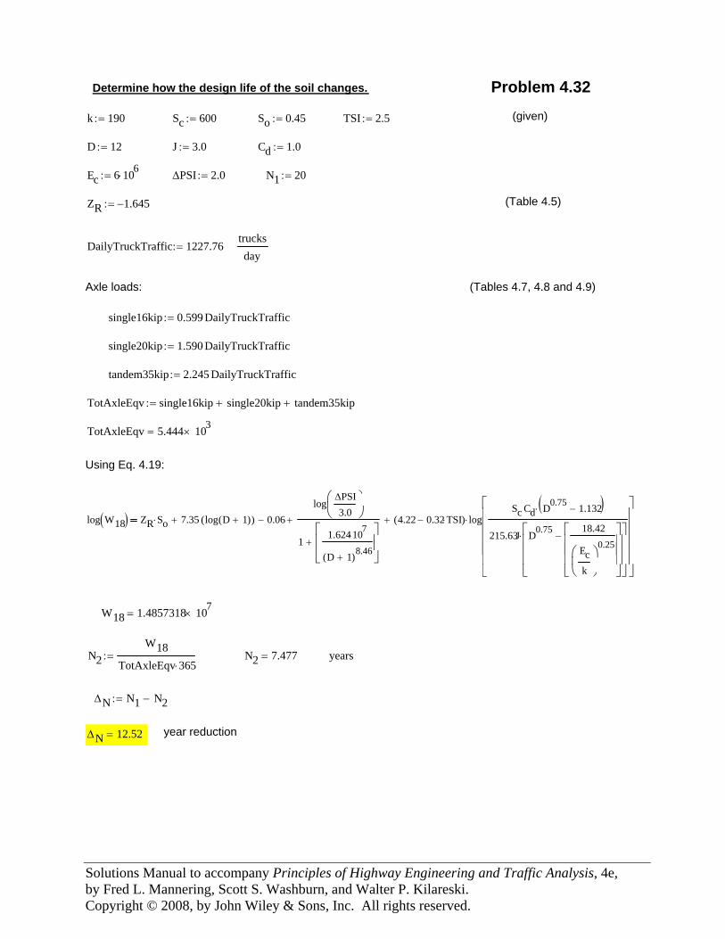
Solutions Manual to accompany Principles of Highway Engineering and Traffic Analysis, 4e, by Fred L. Mannering, Scott S. Washburn, and Walter P. Kilareski. Copyright © 2008, by John Wiley & Sons, Inc. All rights reserved.
Using Eq. 4.19:
TotAxleEqv 5.444 103×=
TotAxleEqv single16kip single20kip+ tandem35kip+:=
tandem35kip 2.245 DailyTruckTraffic⋅:=
single20kip 1.590 DailyTruckTraffic⋅:=
single16kip 0.599 DailyTruckTraffic⋅:=
(Tables 4.7, 4.8 and 4.9)Axle loads:
trucksday
DailyTruckTraffic 1227.76:=
(Table 4.5)ZR 1.645−:=
N1 20:=ΔPSI 2.0:=Ec 6 106⋅:=
Cd 1.0:=J 3.0:=D 12:=
(given) TSI 2.5:=So 0.45:=Sc 600:=k 190:=
Problem 4.32Determine how the design life of the soil changes.
log W18( ) ZR So⋅ 7.35 log D 1+( )( )⋅+ 0.06−
logΔPSI3.0
⎛⎜⎝
⎞⎟⎠
11.624 107⋅
D 1+( )8.46
⎡⎢⎢⎣
⎤⎥⎥⎦
+
+ 4.22 0.32 TSI⋅−( ) logSc Cd D0.75 1.132−( )⋅
215.63J D0.75 18.42
Eck
⎛⎜⎝
⎞⎟⎠
0.25⎡⎢⎢⎢⎣
⎤⎥⎥⎥⎦
−⎡⎢⎢⎢⎣
⎤⎥⎥⎥⎦
⋅
⎡⎢⎢⎢⎢⎢⎣
⎤⎥⎥⎥⎥⎥⎦
⋅+
W18 1.4857318 107×=
N2W18
TotAxleEqv 365⋅:= N2 7.477= years
ΔN N1 N2−:=
ΔN 12.52= year reduction
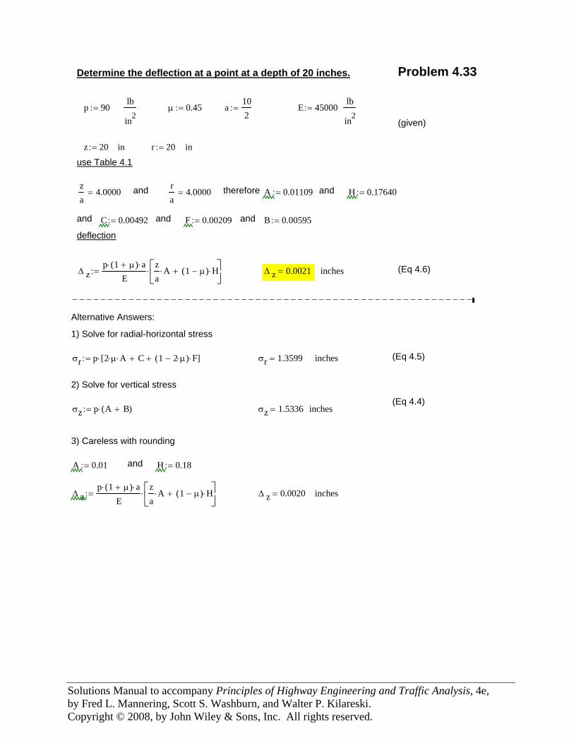
Solutions Manual to accompany Principles of Highway Engineering and Traffic Analysis, 4e, by Fred L. Mannering, Scott S. Washburn, and Walter P. Kilareski. Copyright © 2008, by John Wiley & Sons, Inc. All rights reserved.
Determine the deflection at a point at a depth of 20 inches. Problem 4.33
p 90:=lb
in2μ 0.45:= a
102
:= E 45000:=lb
in2(given)
z 20:= in r 20:= in
use Table 4.1
za
4.0000= and ra
4.0000= therefore A 0.01109:= and H 0.17640:=
and C 0.00492:= and F 0.00209:= and B 0.00595:=
deflection
Δ zp 1 μ+( )⋅ a⋅
Eza
A⋅ 1 μ−( ) H⋅+⎡⎢⎣
⎤⎥⎦
⋅:= Δ z 0.0021= inches (Eq 4.6)
−−−−−−−−−−−−−−−−−−−−−−−−−−−−−−−−−−−−−−−−−−−−−−−−−−−−−−−−− −−−−−−−−−−−−−−−−−−−−−−−−−−−−−−−−−−−−−−−−−−−−−−−−−−−−Alternative Answers:
1) Solve for radial-horizontal stress
σr p 2 μ⋅ A⋅ C+ 1 2 μ⋅−( ) F⋅+[ ]⋅:= σr 1.3599= inches (Eq 4.5)
2) Solve for vertical stress
(Eq 4.4)σz p A B+( )⋅:= σz 1.5336= inches
3) Careless with rounding
A 0.01:= and H 0.18:=
Δ zp 1 μ+( )⋅ a⋅
Eza
A⋅ 1 μ−( ) H⋅+⎡⎢⎣
⎤⎥⎦
⋅:= Δ z 0.0020= inches
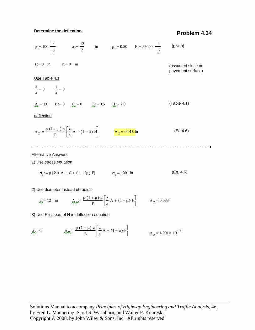
Solutions Manual to accompany Principles of Highway Engineering and Traffic Analysis, 4e, by Fred L. Mannering, Scott S. Washburn, and Walter P. Kilareski. Copyright © 2008, by John Wiley & Sons, Inc. All rights reserved.
Determine the deflection. Problem 4.34
p 100:=lb
in2a
122
:= in μ 0.50:= E 55000:=lb
in2(given)
z 0:= in r 0:= in (assumed since onpavement surface)
Use Table 4.1
za
0=ra
0=
A 1.0:= B 0:= C 0:= F 0.5:= H 2.0:= (Table 4.1)
deflection
Δ zp 1 μ+( )⋅ a⋅
Eza
A⋅ 1 μ−( ) H⋅+⎡⎢⎣
⎤⎥⎦
⋅:= Δ z 0.016= in (Eq 4.6)
−−−−−−−−−−−−−−−−−−−−−−−−−−−−−−−−−−−−−−−−−−−−−−−−−−−−−−−−−−−−−−−−−−−−−−−−−−−−−−−−−−−−−−−−−−−−−−−−−−−−−−−−−−−−
Alternative Answers
1) Use stress equation
σr p 2 μ⋅ A⋅ C+ 1 2μ−( ) F⋅+[ ]⋅:= σr 100= in (Eq. 4.5)
2) Use diameter instead of radius
a 12:= in Δ zp 1 μ+( )⋅ a⋅
Eza
A⋅ 1 μ−( ) H⋅+⎡⎢⎣
⎤⎥⎦
⋅:= Δ z 0.033=
3) Use F instead of H in deflection equation
a 6:= Δ zp 1 μ+( )⋅ a⋅
Eza
A⋅ 1 μ−( ) F⋅+⎡⎢⎣
⎤⎥⎦
⋅:=Δ z 4.091 10 3−
×=
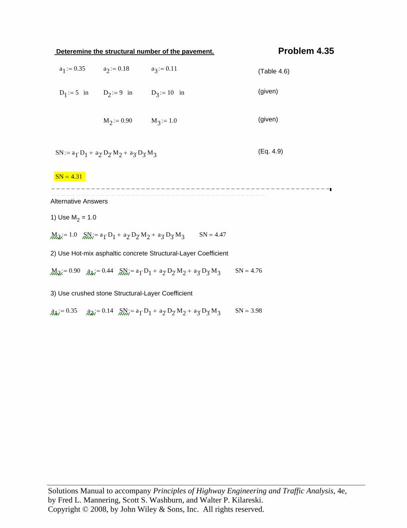
Solutions Manual to accompany Principles of Highway Engineering and Traffic Analysis, 4e, by Fred L. Mannering, Scott S. Washburn, and Walter P. Kilareski. Copyright © 2008, by John Wiley & Sons, Inc. All rights reserved.
Deteremine the structural number of the pavement. Problem 4.35
a1 0.35:= a2 0.18:= a3 0.11:= (Table 4.6)
D1 5:= in D2 9:= in D3 10:= in (given)
M2 0.90:= M3 1.0:= (given)
SN a1 D1⋅ a2 D2⋅ M2⋅+ a3 D3⋅ M3⋅+:= (Eq. 4.9)
SN 4.31=
−−−−−−−−−−−−−−−−−−−−−−−−−−−−−−−−−−−−−−−−−−−−−−−−−−−−−−−− −−−−−−−−−−−−−−−−−−−−−−−−−−−−−−−−−−−−−−−−−−−−Alternative Answers
1) Use M2 = 1.0
M2 1.0:= SN a1 D1⋅ a2 D2⋅ M2⋅+ a3 D3⋅ M3⋅+:= SN 4.47=
2) Use Hot-mix asphaltic concrete Structural-Layer Coefficient
M2 0.90:= a1 0.44:= SN a1 D1⋅ a2 D2⋅ M2⋅+ a3 D3⋅ M3⋅+:= SN 4.76=
3) Use crushed stone Structural-Layer Coefficient
a1 0.35:= a2 0.14:= SN a1 D1⋅ a2 D2⋅ M2⋅+ a3 D3⋅ M3⋅+:= SN 3.98=
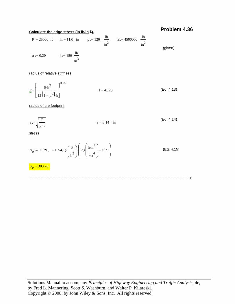
Solutions Manual to accompany Principles of Highway Engineering and Traffic Analysis, 4e, by Fred L. Mannering, Scott S. Washburn, and Walter P. Kilareski. Copyright © 2008, by John Wiley & Sons, Inc. All rights reserved.
Problem 4.36Calculate the edge stress (in lb/in 2).
P 25000:= lb h 11.0:= in p 120:=lb
in2E 4500000:=
lb
in2(given)
μ 0.20:= k 180:=lb
in3
radius of relative stiffness
lE h3⋅
12 1 μ2
−( )⋅ k⋅
⎡⎢⎢⎣
⎤⎥⎥⎦
0.25
:= l 41.23= (Eq. 4.13)
radius of tire footprint
(Eq. 4.14)a
Pp π⋅
:= a 8.14= in
stress
σe 0.529 1 0.54 μ⋅+( )⋅P
h2⎛⎜⎝
⎞⎟⎠
⋅ logE h3⋅
k a4⋅
⎛⎜⎜⎝
⎞⎟⎟⎠
0.71−⎛⎜⎜⎝
⎞⎟⎟⎠
⋅:= (Eq. 4.15)
σe 383.76=
−−−−−−−−−−−−−−−−−−−−−−−−−−−−−−−−−−−−−−−−−−−−−−−−−−−−−−−−
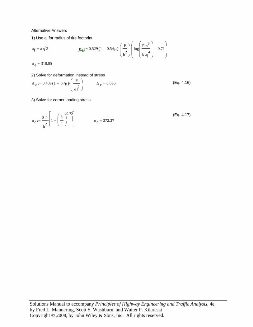
Solutions Manual to accompany Principles of Highway Engineering and Traffic Analysis, 4e, by Fred L. Mannering, Scott S. Washburn, and Walter P. Kilareski. Copyright © 2008, by John Wiley & Sons, Inc. All rights reserved.
−−−−−−−−−−−−−−−−−−−−−−−−−−−−−−−−−−−−−−−−−−−−−−−−−−−−Alternative Answers
1) Use al for radius of tire footprint
al a 2⋅:= σe 0.529 1 0.54 μ⋅+( )⋅P
h2⎛⎜⎝
⎞⎟⎠
⋅ logE h3⋅
k al4
⋅
⎛⎜⎜⎝
⎞⎟⎟⎠
0.71−⎛⎜⎜⎝
⎞⎟⎟⎠
⋅:=
σe 310.85=
2) Solve for deformation instead of stress
Δ e 0.408 1 0.4μ+( )⋅P
k l2⋅
⎛⎜⎝
⎞⎟⎠
⋅:= Δ e 0.036= (Eq. 4.16)
3) Solve for corner loading stress
(Eq. 4.17)σc
3 P⋅
h21
all
⎛⎜⎝
⎞⎟⎠
0.72
−⎡⎢⎢⎣
⎤⎥⎥⎦
⋅:= σc 372.37=
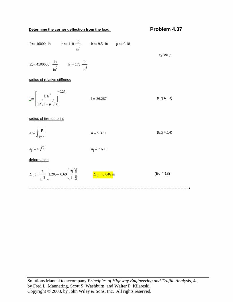
Solutions Manual to accompany Principles of Highway Engineering and Traffic Analysis, 4e, by Fred L. Mannering, Scott S. Washburn, and Walter P. Kilareski. Copyright © 2008, by John Wiley & Sons, Inc. All rights reserved.
Determine the corner deflection from the load. Problem 4.37
P 10000:= lb p 110:=lb
in2h 9.5:= in μ 0.18:=
(given)
E 4100000:=lb
in2k 175:=
lb
in3
radius of relative stiffness
lE h3⋅
12 1 μ2
−( )⋅ k⋅
⎡⎢⎢⎣
⎤⎥⎥⎦
0.25
:= l 36.267= (Eq 4.13)
radius of tire footprint
aP
p π⋅:= a 5.379= (Eq 4.14)
al a 2⋅:= al 7.608=
deformation
Δ cP
k l2⋅1.205 0.69
all
⎛⎜⎝
⎞⎟⎠
⋅−⎡⎢⎣
⎤⎥⎦
⋅:= Δ c 0.046= in (Eq 4.18)
−−−−−−−−−−−−−−−−−−−−−−−−−−−−−−−−−−−−−−−−−−−−−−−−−−−−−−−−
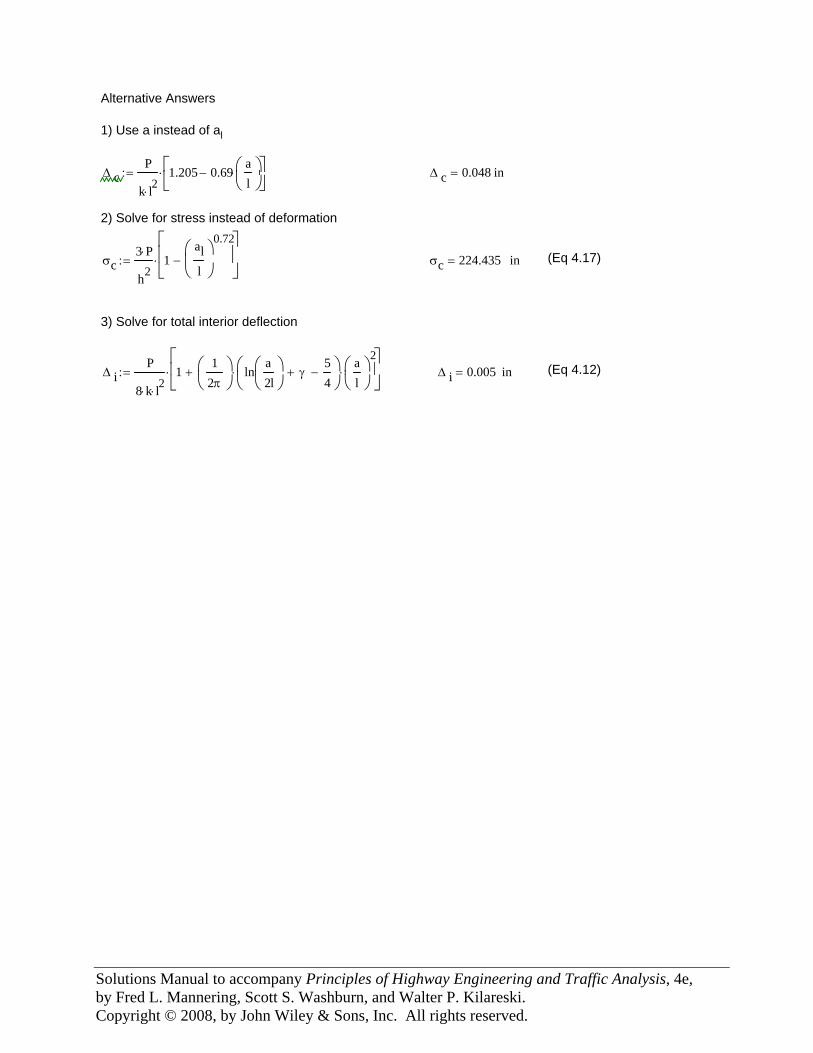
Solutions Manual to accompany Principles of Highway Engineering and Traffic Analysis, 4e, by Fred L. Mannering, Scott S. Washburn, and Walter P. Kilareski. Copyright © 2008, by John Wiley & Sons, Inc. All rights reserved.
−−−−−−−−−−−−−−−−−−−−−−−−−−−−−−−−−−−−−−−−−−−−−−−−−−−Alternative Answers
1) Use a instead of al
Δ cP
k l2⋅1.205 0.69
al
⎛⎜⎝
⎞⎟⎠
⋅−⎡⎢⎣
⎤⎥⎦
⋅:= Δ c 0.048= in
2) Solve for stress instead of deformation
σc3 P⋅
h21
all
⎛⎜⎝
⎞⎟⎠
0.72
−⎡⎢⎢⎣
⎤⎥⎥⎦
⋅:= σc 224.435= in (Eq 4.17)
3) Solve for total interior deflection
Δ iP
8 k⋅ l2⋅1
12π
⎛⎜⎝
⎞⎟⎠
lna2l
⎛⎜⎝
⎞⎟⎠
γ+54
−⎛⎜⎝
⎞⎟⎠
⋅al
⎛⎜⎝
⎞⎟⎠
2⋅+
⎡⎢⎣
⎤⎥⎦
⋅:= Δ i 0.005= in (Eq 4.12)
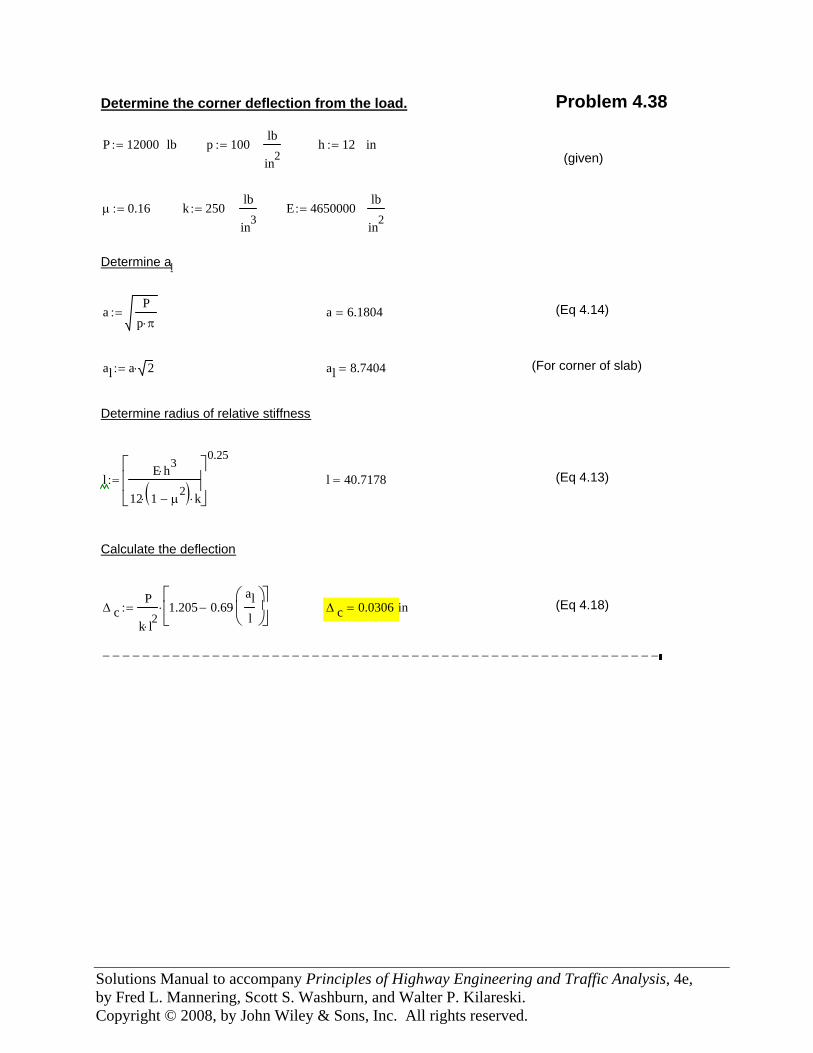
Solutions Manual to accompany Principles of Highway Engineering and Traffic Analysis, 4e, by Fred L. Mannering, Scott S. Washburn, and Walter P. Kilareski. Copyright © 2008, by John Wiley & Sons, Inc. All rights reserved.
Determine the corner deflection from the load. Problem 4.38
P 12000:= lb p 100:=lb
in2h 12:= in
(given)
μ 0.16:= k 250:=lb
in3E 4650000:=
lb
in2
Determine al
aP
p π⋅:= a 6.1804= (Eq 4.14)
al a 2⋅:= al 8.7404= (For corner of slab)
Determine radius of relative stiffness
lE h3⋅
12 1 μ2
−( )⋅ k⋅
⎡⎢⎢⎣
⎤⎥⎥⎦
0.25
:= l 40.7178= (Eq 4.13)
Calculate the deflection
Δ cP
k l2⋅1.205 0.69
all
⎛⎜⎝
⎞⎟⎠
⋅−⎡⎢⎣
⎤⎥⎦
⋅:= Δ c 0.0306= in (Eq 4.18)
−−−−−−−−−−−−−−−−−−−−−−−−−−−−−−−−−−−−−−−−−−−−−−−−−−−−−−−−
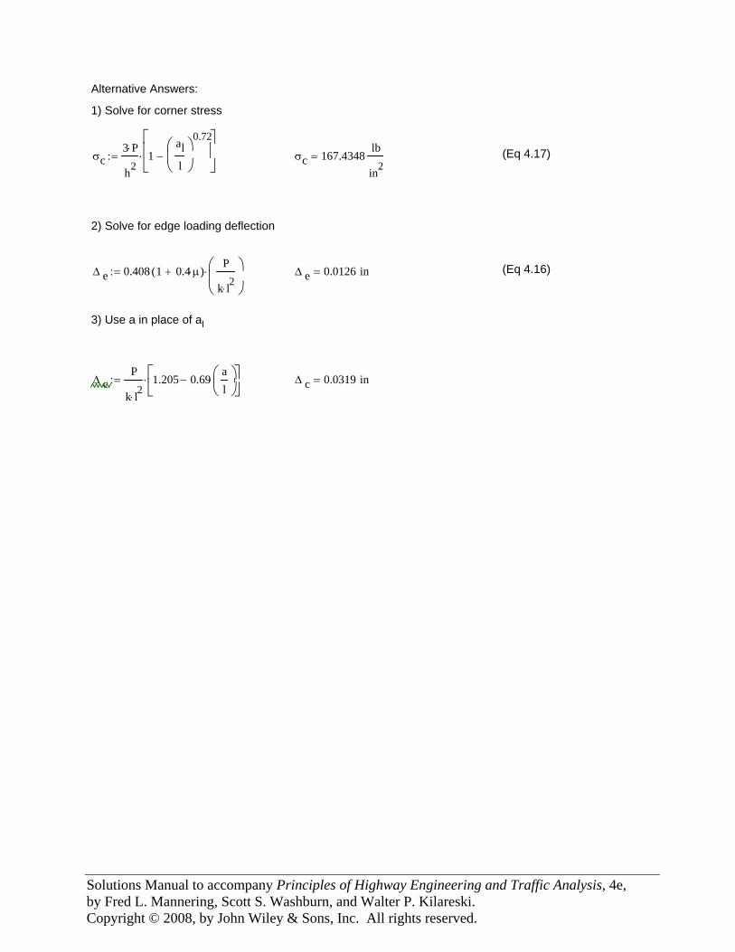
Solutions Manual to accompany Principles of Highway Engineering and Traffic Analysis, 4e, by Fred L. Mannering, Scott S. Washburn, and Walter P. Kilareski. Copyright © 2008, by John Wiley & Sons, Inc. All rights reserved.
Alternative Answers:
1) Solve for corner stress
σc3 P⋅
h21
all
⎛⎜⎝
⎞⎟⎠
0.72
−⎡⎢⎢⎣
⎤⎥⎥⎦
⋅:= σc 167.4348=lb
in2(Eq 4.17)
2) Solve for edge loading deflection
Δ e 0.408 1 0.4 μ⋅+( )⋅P
k l2⋅
⎛⎜⎝
⎞⎟⎠
⋅:= Δ e 0.0126= in (Eq 4.16)
3) Use a in place of al
Δ cP
k l2⋅1.205 0.69
al
⎛⎜⎝
⎞⎟⎠
⋅−⎡⎢⎣
⎤⎥⎦
⋅:= Δ c 0.0319= in
Solutions Manual to accompany
Principles of Highway Engineering and Traffic Analysis, 4e
By Fred L. Mannering, Scott S. Washburn, and Walter P. Kilareski
Chapter 5 Fundamentals of Traffic Flow and
Queuing Theory
U.S. Customary Units
Copyright © 2008, by John Wiley & Sons, Inc. All rights reserved.

Solutions Manual to accompany Principles of Highway Engineering and Traffic Analysis, 4e, by Fred L. Mannering, Scott S. Washburn, and Walter P. Kilareski. Copyright © 2008, by John Wiley & Sons, Inc. All rights reserved.
Preface The solutions to the fourth edition of Principles of Highway Engineering and Traffic Analysis were prepared with the Mathcad1 software program. You will notice several notation conventions that you may not be familiar with if you are not a Mathcad user. Most of these notation conventions are self-explanatory or easily understood. The most common Mathcad specific notations in these solutions relate to the equals sign. You will notice the equals sign being used in three different contexts, and Mathcad uses three different notations to distinguish between each of these contexts. The differences between these equals sign notations are explained as follows.
• The ‘:=’ (colon-equals) is an assignment operator, that is, the value of the variable or expression on the left side of ‘:=’is set equal to the value of the expression on the right side. For example, in the statement, L := 1234, the variable ‘L’ is assigned (i.e., set equal to) the value of 1234. Another example is x := y + z. In this case, x is assigned the value of y + z.
• The ‘==’ (bold equals) is used when the Mathcad function solver was used to find the value of a variable in the equation. For example, in the equation
, the == is used to tell Mathcad that the value of the expression on the left side needs to equal the value of the expression on the right side. Thus, the Mathcad solver can be employed to find a value for the variable ‘t’ that satisfies this relationship. This particular example is from a problem where the function for arrivals at some time ‘t’ is set equal to the function for departures at some time ‘t’ to find the time to queue clearance.
• The ‘=’ (standard equals) is used for a simple numeric evaluation. For example, referring to the x := y + z assignment used previously, if the value of y was 10 [either by assignment (with :=), or the result of an equation solution (through the use of ==) and the value of z was 15, then the expression ‘x =’ would yield 25. Another example would be as follows: s := 1800/3600, with s = 0.5. That is, ‘s’ was assigned the value of 1800 divided by 3600 (using :=), which equals 0.5 (as given by using =).
Another symbol you will see frequently is ‘→’. In these solutions, it is used to perform an evaluation of an assignment expression in a single statement. For example, in the following
statement, , Q(t) is assigned the value of Arrivals(t) – Departures(t), and this evaluates to 2.2t – 0.10t2. Finally, to assist in quickly identifying the final answer, or answers, for what is being asked in the problem statement, yellow highlighting has been used (which will print as light gray). 1 www.mathcad.com
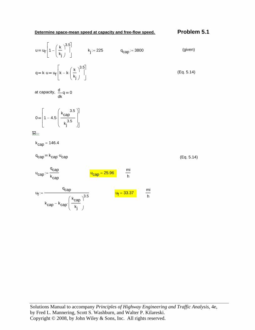
Solutions Manual to accompany Principles of Highway Engineering and Traffic Analysis, 4e, by Fred L. Mannering, Scott S. Washburn, and Walter P. Kilareski. Copyright © 2008, by John Wiley & Sons, Inc. All rights reserved.
Determine space-mean speed at capacity and free-flow speed. Problem 5.1
u uf 1kkj
⎛⎜⎝
⎞⎟⎠
3.5−
⎡⎢⎢⎣
⎤⎥⎥⎦
⋅ kj 225:= qcap 3800:= (given)
q k u⋅ uf k kkkj
⎛⎜⎝
⎞⎟⎠
3.5⋅−
⎡⎢⎢⎣
⎤⎥⎥⎦
⋅ (Eq. 5.14)
at capacity, k
qdd
0
0 1 4.5kcap
3.5
kj3.5
⎛⎜⎜⎝
⎞⎟⎟⎠
⋅−
⎡⎢⎢⎣
⎤⎥⎥⎦
kcap 146.4=
qcap kcap ucap⋅ (Eq. 5.14)
ucapqcapkcap
:= ucap 25.96=mih
ufqcap
kcap kcapkcap
kj
⎛⎜⎜⎝
⎞⎟⎟⎠
3.5
⋅−
:= uf 33.37=mih
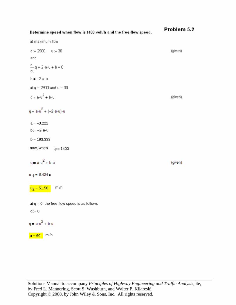
Solutions Manual to accompany Principles of Highway Engineering and Traffic Analysis, 4e, by Fred L. Mannering, Scott S. Washburn, and Walter P. Kilareski. Copyright © 2008, by John Wiley & Sons, Inc. All rights reserved.
a 3.222−=
b 2− a⋅ u⋅:=
b 193.333=
now, when q 1400:=
u2 51.58= mi/h
at q = 0, the free flow speed is as follows
q 0:=
u 60= mi/h
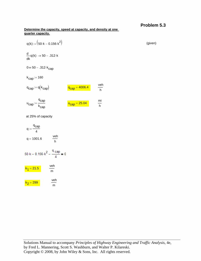
Solutions Manual to accompany Principles of Highway Engineering and Traffic Analysis, 4e, by Fred L. Mannering, Scott S. Washburn, and Walter P. Kilareski. Copyright © 2008, by John Wiley & Sons, Inc. All rights reserved.
vehh
q 1001.6=
qqcap
4:=
at 25% of capacity
mih
ucap 25.04=ucapqcapkcap
:=
vehh
qcap 4006.4=qcap q kcap( ):=
kcap 160:=
0 50 .312 kcap⋅−
kq k( )d
d50 .312 k⋅−→
(given)q k( ) 50 k⋅ 0.156 k2⋅−( ):=
Determine the capacity, speed at capacity, and density at one quarter capacity.
Problem 5.3
k1 21.5=vehm
k2 299=vehm
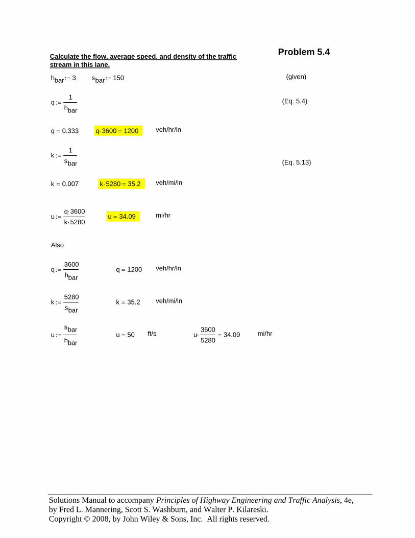
Solutions Manual to accompany Principles of Highway Engineering and Traffic Analysis, 4e, by Fred L. Mannering, Scott S. Washburn, and Walter P. Kilareski. Copyright © 2008, by John Wiley & Sons, Inc. All rights reserved.
mi/hru36005280⋅ 34.09=ft/su 50=u
sbarhbar
:=
veh/mi/lnk 35.2=k5280sbar
:=
veh/hr/ln q 1200=q3600hbar
:=
Also
mi/hru 34.09=uq 3600⋅
k 5280⋅:=
veh/mi/lnk 5280⋅ 35.2=k 0.007=
(Eq. 5.13)k
1sbar
:=
veh/hr/ln q 3600⋅ 1200=q 0.333=
(Eq. 5.4)q1
hbar:=
(given)sbar 150:=hbar 3:=
Calculate the flow, average speed, and density of the trafficstream in this lane.
Problem 5.4
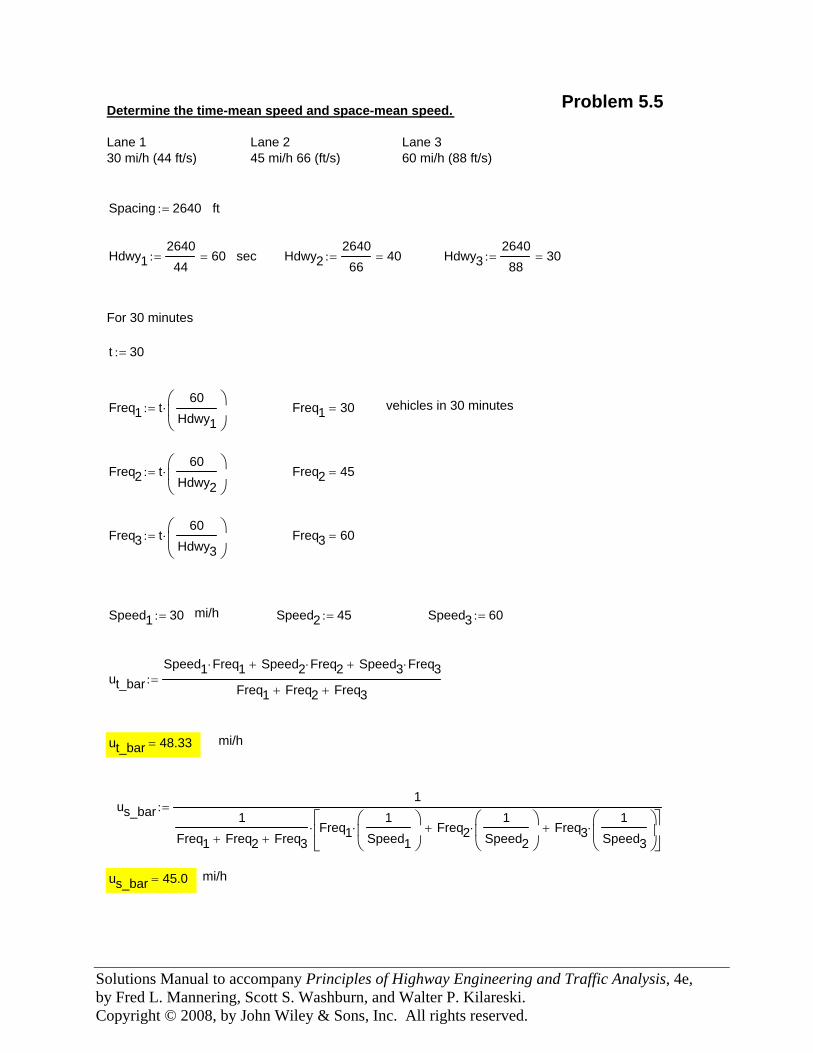
Solutions Manual to accompany Principles of Highway Engineering and Traffic Analysis, 4e, by Fred L. Mannering, Scott S. Washburn, and Walter P. Kilareski. Copyright © 2008, by John Wiley & Sons, Inc. All rights reserved.
Problem 5.5Determine the time-mean speed and space-mean speed.
Lane 130 mi/h (44 ft/s)
Lane 245 mi/h 66 (ft/s)
Lane 360 mi/h (88 ft/s)
Spacing 2640:= ft
Hdwy1264044
60=:= sec Hdwy2264066
40=:= Hdwy3264088
30=:=
For 30 minutes
t 30:=
Freq1 t60
Hdwy1
⎛⎜⎝
⎞⎟⎠
⋅:= Freq1 30= vehicles in 30 minutes
Freq2 t60
Hdwy2
⎛⎜⎝
⎞⎟⎠
⋅:= Freq2 45=
Freq3 t60
Hdwy3
⎛⎜⎝
⎞⎟⎠
⋅:= Freq3 60=
Speed1 30:= mi/h Speed2 45:= Speed3 60:=
ut_barSpeed1 Freq1⋅ Speed2 Freq2⋅+ Speed3 Freq3⋅+
Freq1 Freq2+ Freq3+:=
ut_bar 48.33= mi/h
us_bar1
1Freq1 Freq2+ Freq3+
Freq11
Speed1
⎛⎜⎝
⎞⎟⎠
⋅ Freq21
Speed2
⎛⎜⎝
⎞⎟⎠
⋅+ Freq31
Speed3
⎛⎜⎝
⎞⎟⎠
⋅+⎡⎢⎣
⎤⎥⎦
⋅
:=
us_bar 45.0= mi/h
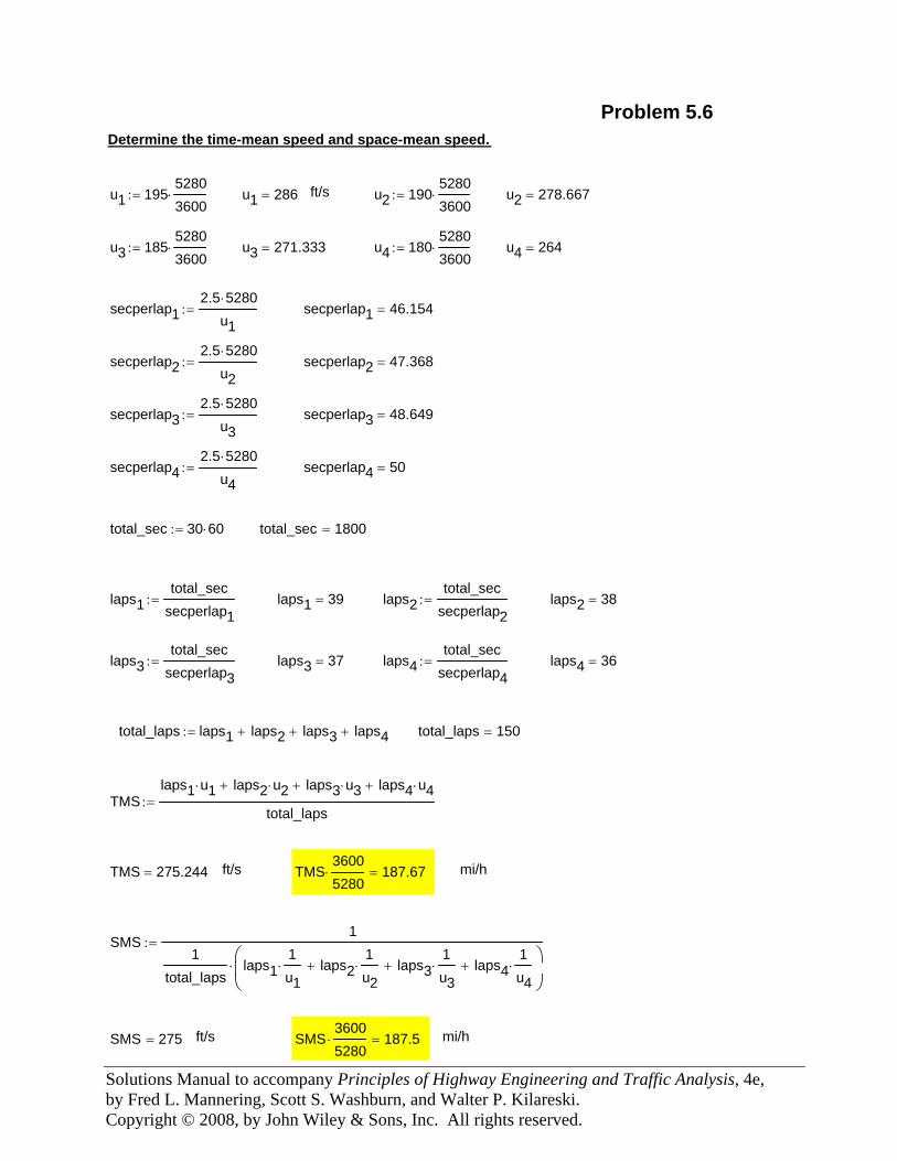
Solutions Manual to accompany Principles of Highway Engineering and Traffic Analysis, 4e, by Fred L. Mannering, Scott S. Washburn, and Walter P. Kilareski. Copyright © 2008, by John Wiley & Sons, Inc. All rights reserved.
laps1total_sec
secperlap1:= laps1 39= laps2
total_secsecperlap2
:= laps2 38=
laps3total_sec
secperlap3:= laps3 37= laps4
total_secsecperlap4
:= laps4 36=
total_laps laps1 laps2+ laps3+ laps4+:= total_laps 150=
TMSlaps1 u1⋅ laps2 u2⋅+ laps3 u3⋅+ laps4 u4⋅+
total_laps:=
TMS 275.244= ft/s TMS36005280⋅ 187.67= mi/h
SMS1
1total_laps
laps11u1⋅ laps2
1u2⋅+ laps3
1u3⋅+ laps4
1u4⋅+
⎛⎜⎝
⎞⎟⎠
⋅
:=
SMS 275= ft/s SMS36005280⋅ 187.5= mi/h
Problem 5.6Determine the time-mean speed and space-mean speed.
u1 19552803600⋅:= u1 286= ft/s u2 190
52803600⋅:= u2 278.667=
u3 18552803600⋅:= u3 271.333= u4 180
52803600⋅:= u4 264=
secperlap12.5 5280⋅
u1:= secperlap1 46.154=
secperlap22.5 5280⋅
u2:= secperlap2 47.368=
secperlap32.5 5280⋅
u3:= secperlap3 48.649=
secperlap42.5 5280⋅
u4:= secperlap4 50=
total_sec 30 60⋅:= total_sec 1800=
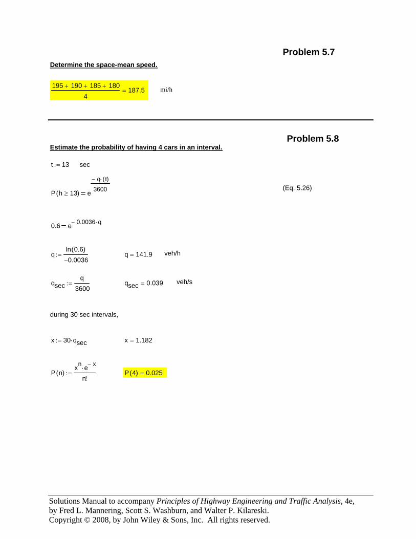
Solutions Manual to accompany Principles of Highway Engineering and Traffic Analysis, 4e, by Fred L. Mannering, Scott S. Washburn, and Walter P. Kilareski. Copyright © 2008, by John Wiley & Sons, Inc. All rights reserved.
Problem 5.7Determine the space-mean speed.
195 190+ 185+ 180+
4187.5= mi/h
P 4( ) 0.025=P n( )xn e x−
⋅
n!:=
x 1.182=x 30 qsec⋅:=
during 30 sec intervals,
veh/sqsec 0.039=qsecq
3600:=
veh/hq 141.9=qln 0.6( )0.0036−
:=
0.6 e 0.0036− q⋅
P h 13≥( ) e
q− t( )⋅
3600 (Eq. 5.26)
sect 13:=
Estimate the probability of having 4 cars in an interval.Problem 5.8
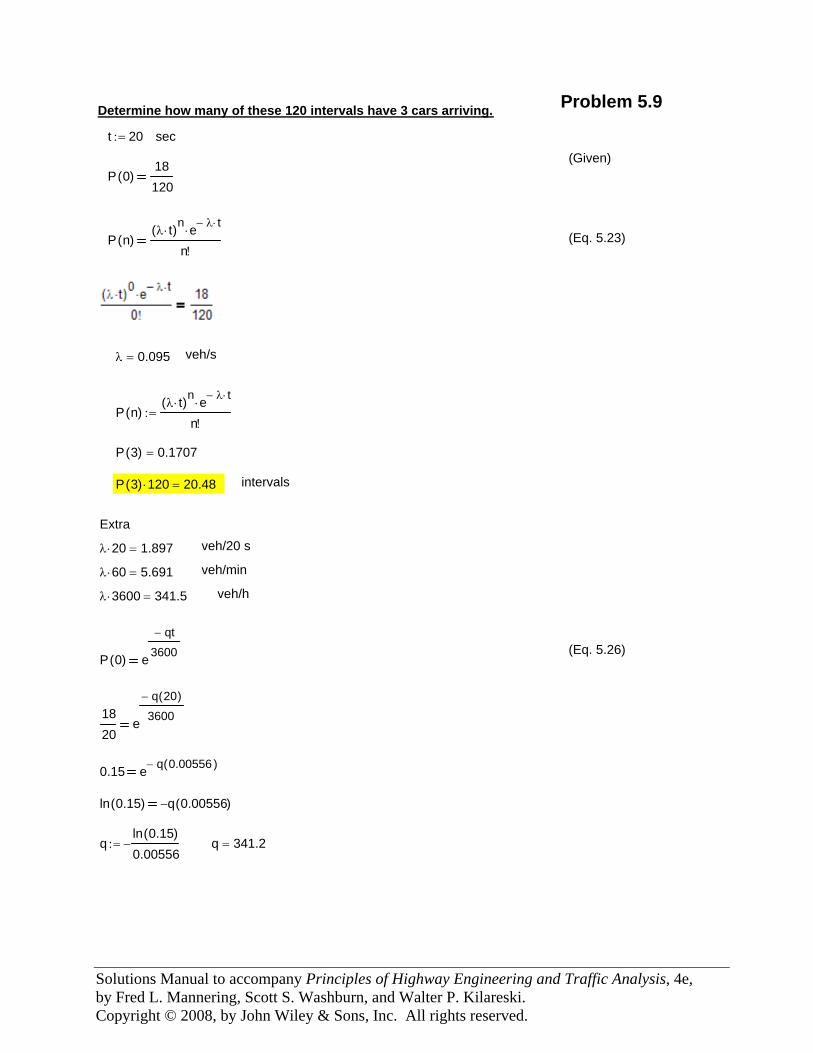
Solutions Manual to accompany Principles of Highway Engineering and Traffic Analysis, 4e, by Fred L. Mannering, Scott S. Washburn, and Walter P. Kilareski. Copyright © 2008, by John Wiley & Sons, Inc. All rights reserved.
Problem 5.9Determine how many of these 120 intervals have 3 cars arriving.
t 20:= sec
(Given)P 0( )
18120
P n( )λ t⋅( )n e λ− t⋅
⋅
n!(Eq. 5.23)
q 341.2=qln 0.15( )0.00556
−:=
ln 0.15( ) q 0.00556( )−
0.15 e q 0.00556( )−
1820
e
q 20( )−
3600
P 0( ) e
qt−
3600 (Eq. 5.26)
veh/hλ 3600⋅ 341.5=
veh/minλ 60⋅ 5.691=
veh/20 sλ 20⋅ 1.897=
Extra
intervalsP 3( ) 120⋅ 20.48=
P 3( ) 0.1707=
P n( )λ t⋅( )n e λ− t⋅
⋅
n!:=
veh/sλ 0.095=
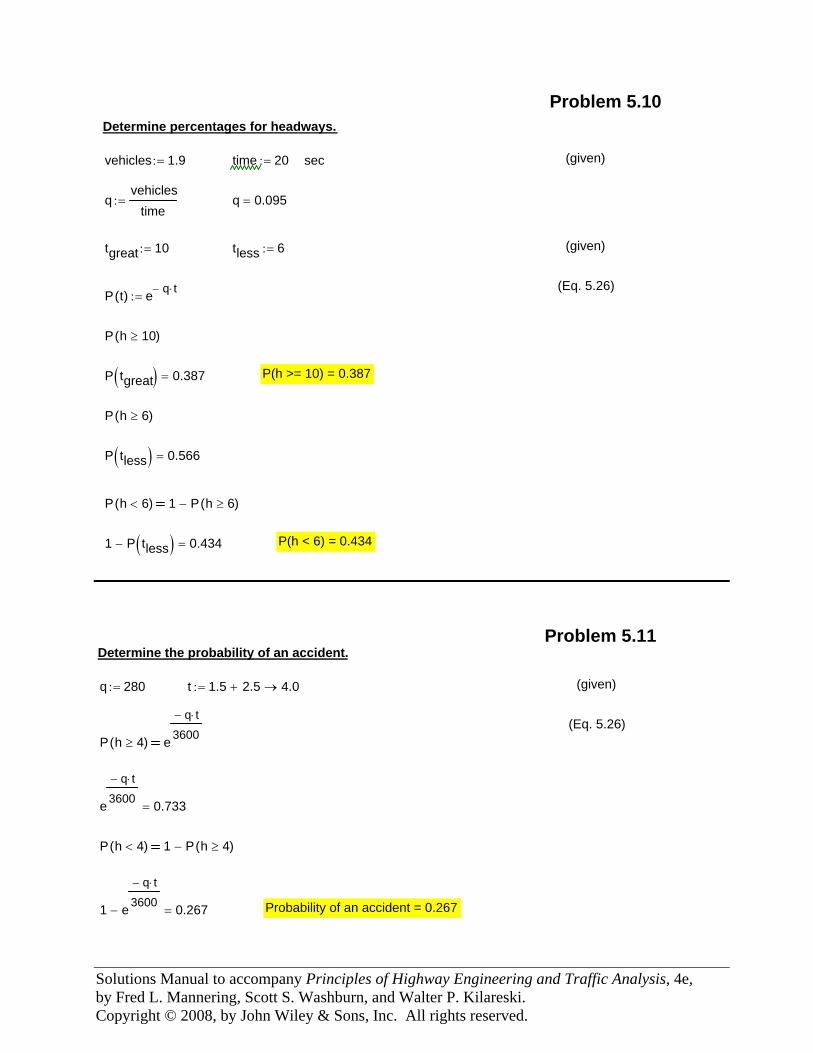
Solutions Manual to accompany Principles of Highway Engineering and Traffic Analysis, 4e, by Fred L. Mannering, Scott S. Washburn, and Walter P. Kilareski. Copyright © 2008, by John Wiley & Sons, Inc. All rights reserved.
Problem 5.10Determine percentages for headways.
vehicles 1.9:= time 20:= sec (given)
qvehicles
time:= q 0.095=
tgreat 10:= tless 6:= (given)
(Eq. 5.26)P t( ) e q− t⋅
:=
P h 10≥( )
P tgreat( ) 0.387= P(h >= 10) = 0.387
P h 6≥( )
P tless( ) 0.566=
P h 6<( ) 1 P h 6≥( )−
1 P tless( )− 0.434= P(h < 6) = 0.434
Problem 5.11Determine the probability of an accident.
q 280:= t 1.5 2.5+ 4.0→:= (given)
(Eq. 5.26)P h 4≥( ) e
q− t⋅
3600
e
q− t⋅
3600 0.733=
P h 4<( ) 1 P h 4≥( )−
1 e
q− t⋅
3600− 0.267= Probability of an accident = 0.267
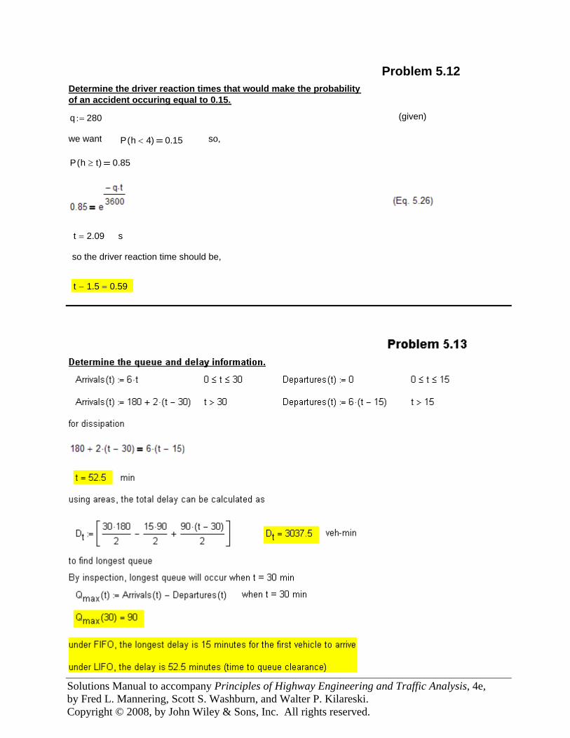
Solutions Manual to accompany Principles of Highway Engineering and Traffic Analysis, 4e, by Fred L. Mannering, Scott S. Washburn, and Walter P. Kilareski. Copyright © 2008, by John Wiley & Sons, Inc. All rights reserved.
Problem 5.12Determine the driver reaction times that would make the probabilityof an accident occuring equal to 0.15.
q 280:= (given)
we want P h 4<( ) 0.15 so,
P h t≥( ) 0.85
t 2.09= s
so the driver reaction time should be,
t 1.5− 0.59=
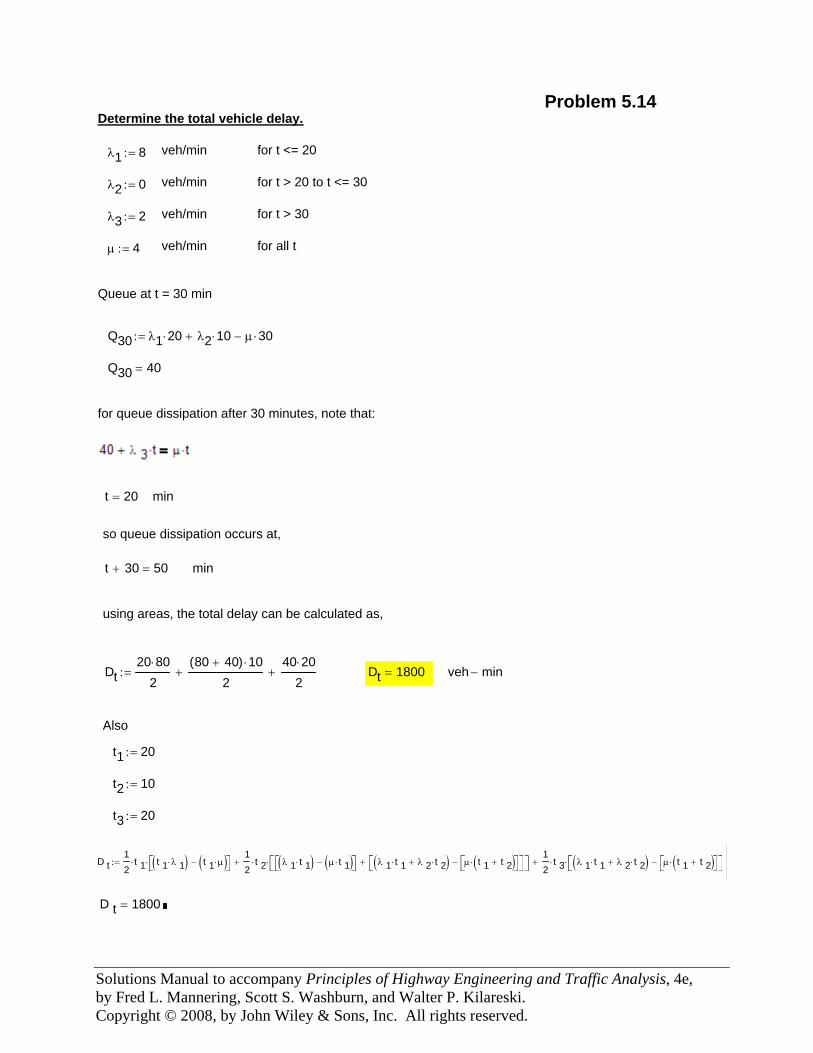
Solutions Manual to accompany Principles of Highway Engineering and Traffic Analysis, 4e, by Fred L. Mannering, Scott S. Washburn, and Walter P. Kilareski. Copyright © 2008, by John Wiley & Sons, Inc. All rights reserved.
for queue dissipation after 30 minutes, note that:
Q30 40=
Q30 λ1 20⋅ λ2 10⋅+ μ 30⋅−:=
Queue at t = 30 min
for all tveh/minμ 4:=
for t > 30veh/minλ3 2:=
for t > 20 to t <= 30veh/minλ2 0:=
for t <= 20veh/minλ1 8:=
Determine the total vehicle delay.Problem 5.14
t 20= min
so queue dissipation occurs at,
t 30+ 50= min
using areas, the total delay can be calculated as,
Dt20 80⋅
280 40+( ) 10⋅
2+
40 20⋅
2+:= Dt 1800= veh min−
Also
t1 20:=
t2 10:=
t3 20:=
D t12
t 1⋅ t 1 λ 1⋅( ) t 1 μ⋅( )−⎡⎣ ⎤⎦⋅12
t 2⋅ λ 1 t 1⋅( ) μ t 1⋅( )−⎡⎣ ⎤⎦ λ 1 t 1⋅ λ 2 t 2⋅+( ) μ t 1 t 2+( )⋅⎡⎣ ⎤⎦−⎡⎣ ⎤⎦+⎡⎣ ⎤⎦⋅+12
t 3⋅ λ 1 t 1⋅ λ 2 t 2⋅+( ) μ t 1 t 2+( )⋅⎡⎣ ⎤⎦−⎡⎣ ⎤⎦⋅+:=
D t 1800=

Solutions Manual to accompany Principles of Highway Engineering and Traffic Analysis, 4e, by Fred L. Mannering, Scott S. Washburn, and Walter P. Kilareski. Copyright © 2008, by John Wiley & Sons, Inc. All rights reserved.
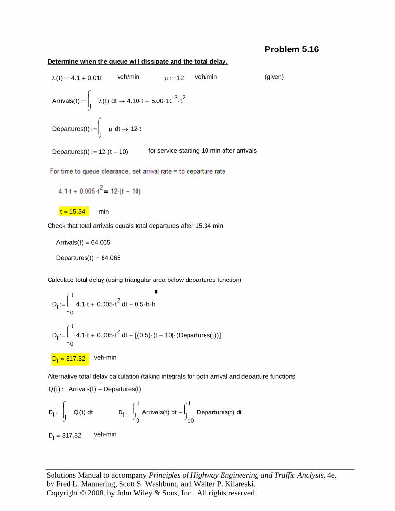
Solutions Manual to accompany Principles of Highway Engineering and Traffic Analysis, 4e, by Fred L. Mannering, Scott S. Washburn, and Walter P. Kilareski. Copyright © 2008, by John Wiley & Sons, Inc. All rights reserved.
Problem 5.16Determine when the queue will dissipate and the total delay.
λ t( ) 4.1 0.01t+:= veh/min μ 12:= veh/min (given)
Arrivals t( ) tλ t( )⌠⎮⎮⌡
d 4.10 t⋅ 5.00 10-3⋅ t2⋅+→:=
Departures t( ) tμ⌠⎮⎮⌡
d 12 t⋅→:=
Departures t( ) 12 t 10−( )⋅:= for service starting 10 min after arrivals
t 15.34= min
Check that total arrivals equals total departures after 15.34 min
Arrivals t( ) 64.065=
Departures t( ) 64.065=
Calculate total delay (using triangular area below departures function)
Dt0
t
t4.1 t⋅ 0.005 t2⋅+⌠⎮⌡
d 0.5 b⋅ h⋅−:=
Dt0
t
t4.1 t⋅ 0.005 t2⋅+⌠⎮⌡
d 0.5( ) t 10−( )⋅ Departures t( )( )⋅[ ]−:=
Dt 317.32= veh-min
Alternative total delay calculation (taking integrals for both arrival and departure functions)
Q t( ) Arrivals t( ) Departures t( )−:=
Dt tQ t( )⌠⎮⎮⌡
d:= Dt0
ttArrivals t( )
⌠⎮⌡
d10
ttDepartures t( )
⌠⎮⌡
d−:=
Dt 317.32= veh-min
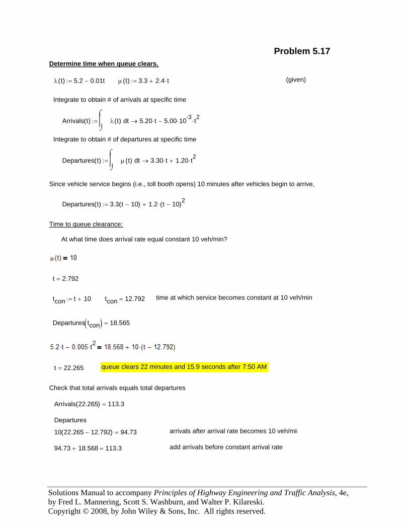
Solutions Manual to accompany Principles of Highway Engineering and Traffic Analysis, 4e, by Fred L. Mannering, Scott S. Washburn, and Walter P. Kilareski. Copyright © 2008, by John Wiley & Sons, Inc. All rights reserved.
Problem 5.17Determine time when queue clears.
λ t( ) 5.2 0.01t−:= μ t( ) 3.3 2.4 t⋅+:= (given)
Integrate to obtain # of arrivals at specific time
Arrivals t( ) tλ t( )⌠⎮⎮⌡
d 5.20 t⋅ 5.00 10-3⋅ t2⋅−→:=
Integrate to obtain # of departures at specific time
Departures t( ) tμ t( )⌠⎮⎮⌡
d 3.30 t⋅ 1.20 t2⋅+→:=
Since vehicle service begins (i.e., toll booth opens) 10 minutes after vehicles begin to arrive,
Departures t( ) 3.3 t 10−( ) 1.2 t 10−( )2⋅+:=
Time to queue clearance:
At what time does arrival rate equal constant 10 veh/min?
t 2.792=
tcon t 10+:= tcon 12.792= time at which service becomes constant at 10 veh/min
Departures tcon( ) 18.565=
t 22.265= queue clears 22 minutes and 15.9 seconds after 7:50 AM
Check that total arrivals equals total departures
Arrivals 22.265( ) 113.3=
Departures
10 22.265 12.792−( ) 94.73= arrivals after arrival rate becomes 10 veh/min
94.73 18.568+ 113.3= add arrivals before constant arrival rate
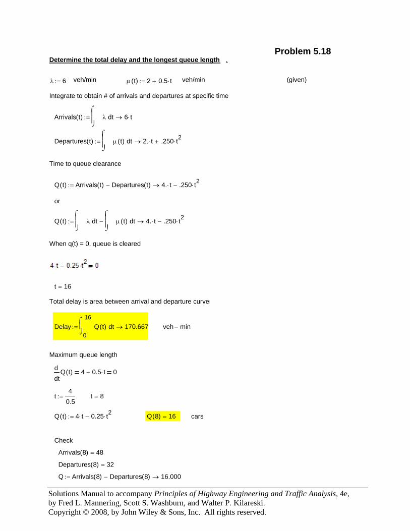
Solutions Manual to accompany Principles of Highway Engineering and Traffic Analysis, 4e, by Fred L. Mannering, Scott S. Washburn, and Walter P. Kilareski. Copyright © 2008, by John Wiley & Sons, Inc. All rights reserved.
Problem 5.18Determine the total delay and the longest queue length .
λ 6:= veh/min μ t( ) 2 0.5 t⋅+:= veh/min (given)
Integrate to obtain # of arrivals and departures at specific time
Arrivals t( ) tλ⌠⎮⎮⌡
d 6 t⋅→:=
Departures t( ) tμ t( )⌠⎮⎮⌡
d 2. t⋅ .250 t2⋅+→:=
Time to queue clearance
Q t( ) Arrivals t( ) Departures t( )− 4. t⋅ .250 t2⋅−→:=
or
Q t( ) tλ⌠⎮⎮⌡
d tμ t( )⌠⎮⎮⌡
d− 4. t⋅ .250 t2⋅−→:=
When q(t) = 0, queue is cleared
t 16=
Total delay is area between arrival and departure curves
Delay0
16tQ t( )
⌠⎮⌡
d 170.667→:= veh min−
Maximum queue length
tQ t( )d
d4 0.5 t⋅− 0
t4
0.5:= t 8=
Q t( ) 4 t⋅ 0.25 t2⋅−:= Q 8( ) 16= cars
Check
Arrivals 8( ) 48=
Departures 8( ) 32=
Q Arrivals 8( ) Departures 8( )− 16.000→:=
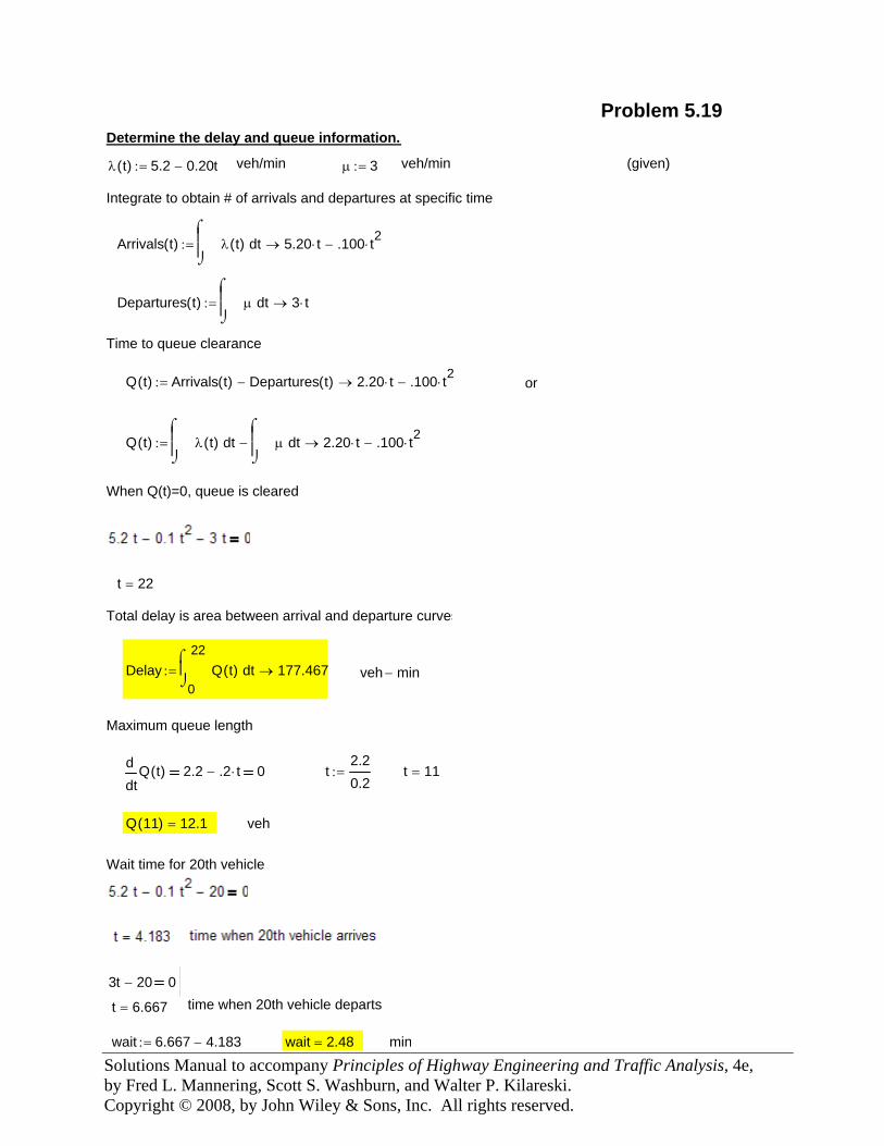
Solutions Manual to accompany Principles of Highway Engineering and Traffic Analysis, 4e, by Fred L. Mannering, Scott S. Washburn, and Walter P. Kilareski. Copyright © 2008, by John Wiley & Sons, Inc. All rights reserved.
Problem 5.19Determine the delay and queue information.
λ t( ) 5.2 0.20t−:= veh/min μ 3:= veh/min (given)
Integrate to obtain # of arrivals and departures at specific time
Arrivals t( ) tλ t( )⌠⎮⎮⌡
d 5.20 t⋅ .100 t2⋅−→:=
Departures t( ) tμ⌠⎮⎮⌡
d 3 t⋅→:=
Time to queue clearance
Q t( ) Arrivals t( ) Departures t( )− 2.20 t⋅ .100 t2⋅−→:= or
Q t( ) tλ t( )⌠⎮⎮⌡
d tμ⌠⎮⎮⌡
d− 2.20 t⋅ .100 t2⋅−→:=
When Q(t)=0, queue is cleared
t 22=
Total delay is area between arrival and departure curves
Delay0
22tQ t( )
⌠⎮⌡
d 177.467→:= veh min−
Maximum queue length
tQ t( )d
d2.2 .2 t⋅− 0 t
2.20.2
:= t 11=
Q 11( ) 12.1= veh
Wait time for 20th vehicle
3t 20− 0
t 6.667= time when 20th vehicle departs
wait 6.667 4.183−:= wait 2.48= min
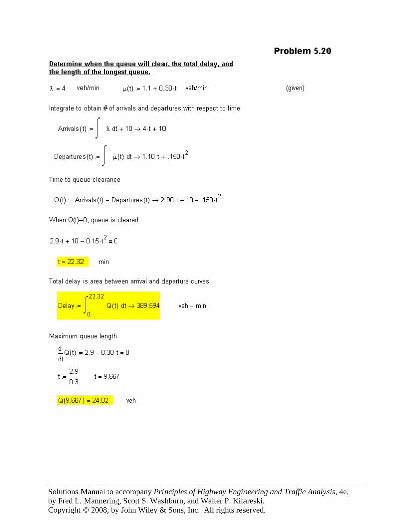
Solutions Manual to accompany Principles of Highway Engineering and Traffic Analysis, 4e, by Fred L. Mannering, Scott S. Washburn, and Walter P. Kilareski. Copyright © 2008, by John Wiley & Sons, Inc. All rights reserved.
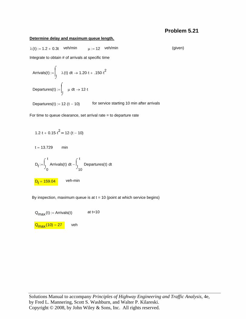
Solutions Manual to accompany Principles of Highway Engineering and Traffic Analysis, 4e, by Fred L. Mannering, Scott S. Washburn, and Walter P. Kilareski. Copyright © 2008, by John Wiley & Sons, Inc. All rights reserved.
vehQmax 10( ) 27=
at t=10Qmax t( ) Arrivals t( ):=
By inspection, maximum queue is at t = 10 (point at which service begins)
veh-minDt 159.04=
Dt0
ttArrivals t( )
⌠⎮⌡
d10
ttDepartures t( )
⌠⎮⌡
d−:=
mint 13.729=
1.2 t⋅ 0.15 t2⋅+ 12 t 10−( )⋅
For time to queue clearance, set arrival rate = to departure rate
for service starting 10 min after arrivalsDepartures t( ) 12 t 10−( )⋅:=
Departures t( ) tμ⌠⎮⎮⌡
d 12 t⋅→:=
Arrivals t( ) tλ t( )⌠⎮⎮⌡
d 1.20 t⋅ .150 t2⋅+→:=
Integrate to obtain # of arrivals at specific time
(given)veh/minμ 12:=veh/minλ t( ) 1.2 0.3t+:=
Determine delay and maximum queue length.
Problem 5.21
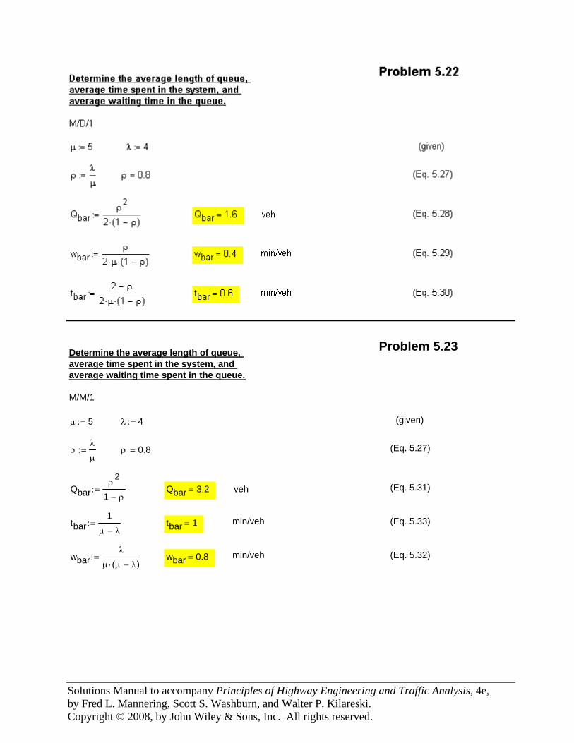
Solutions Manual to accompany Principles of Highway Engineering and Traffic Analysis, 4e, by Fred L. Mannering, Scott S. Washburn, and Walter P. Kilareski. Copyright © 2008, by John Wiley & Sons, Inc. All rights reserved.
(Eq. 5.32)min/vehwbar 0.8=wbarλ
μ μ λ−( )⋅:=
(Eq. 5.33)min/vehtbar 1=tbar1
μ λ−:=
(Eq. 5.31)vehQbar 3.2=Qbarρ
2
1 ρ−:=
(Eq. 5.27)ρ 0.8=ρλ
μ:=
(given)λ 4:=μ 5:=
M/M/1
Determine the average length of queue, average time spent in the system, and average waiting time spent in the queue.
Problem 5.23
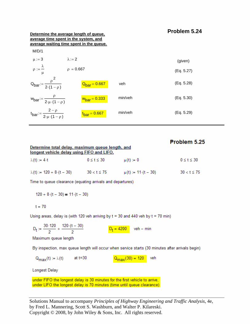
Solutions Manual to accompany Principles of Highway Engineering and Traffic Analysis, 4e, by Fred L. Mannering, Scott S. Washburn, and Walter P. Kilareski. Copyright © 2008, by John Wiley & Sons, Inc. All rights reserved.
(Eq. 5.29)min/vehtbar 0.667=tbar2 ρ−
2 μ⋅ 1 ρ−( )⋅:=
(Eq. 5.30)min/vehwbar 0.333=wbarρ
2 μ⋅ 1 ρ−( )⋅:=
(Eq. 5.28)vehQbar 0.667=Qbarρ
2
2 1 ρ−( )⋅:=
(Eq. 5.27)ρ 0.667=ρλ
μ:=
(given)λ 2:=μ 3:=
M/D/1
Determine the average length of queue,average time spent in the system, andaverage waiting time spent in the queue.
Problem 5.24
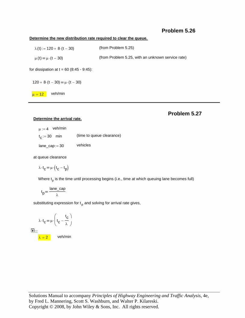
Solutions Manual to accompany Principles of Highway Engineering and Traffic Analysis, 4e, by Fred L. Mannering, Scott S. Washburn, and Walter P. Kilareski. Copyright © 2008, by John Wiley & Sons, Inc. All rights reserved.
Problem 5.26Determine the new distribution rate required to clear the queue.
λ t( ) 120 8 t 30−( )⋅+:= (from Problem 5.25)
μ t( ) μ t 30−( )⋅ (from Problem 5.25, with an unknown service rate)
for dissipation at t = 60 (8:45 - 9:45):
120 8 t 30−( )⋅+ μ t 30−( )⋅
μ 12= veh/min
Problem 5.27Determine the arrival rate.
μ 4:= veh/min
tc 30:= min (time to queue clearance)
lane_cap 30:= vehicles
at queue clearance
λ tc⋅ μ tc tp−( )⋅
Where tp is the time until processing begins (i.e., time at which queuing lane becomes full)
tplane_cap
λ
substituting expression for t p and solving for arrival rate gives,
λ tc⋅ μ tctcλ
−⎛⎜⎝
⎞⎟⎠
⋅
λ 2= veh/min
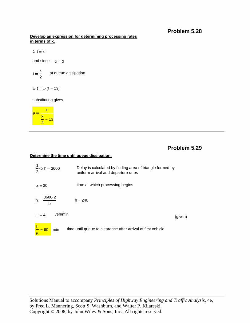
Solutions Manual to accompany Principles of Highway Engineering and Traffic Analysis, 4e, by Fred L. Mannering, Scott S. Washburn, and Walter P. Kilareski. Copyright © 2008, by John Wiley & Sons, Inc. All rights reserved.
Problem 5.28Develop an expression for determining processing ratesin terms of x.
λ t⋅ x
and since λ 2
tx2
at queue dissipation
λ t⋅ μ t 13−( )⋅
substituting gives
μx
x2
13−
Problem 5.29Determine the time until queue dissipation.
12
b⋅ h⋅ 3600 Delay is calculated by finding area of triangle formed by uniform arrival and departure rates
b 30:= time at which processing begins
h3600 2⋅
b:= h 240=
μ 4:= veh/min (given)
hμ
60= min time until queue to clearance after arrival of first vehicle
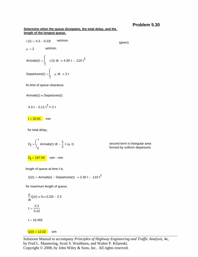
Solutions Manual to accompany Principles of Highway Engineering and Traffic Analysis, 4e, by Fred L. Mannering, Scott S. Washburn, and Walter P. Kilareski. Copyright © 2008, by John Wiley & Sons, Inc. All rights reserved.
vehQ t( ) 12.02=
t 10.455=
t2.30.22
:=
tQ t( )d
d0 0.22t 2.3−
for maximum length of queue,
Q t( ) Arrivals t( ) Departures t( )− 2.30 t⋅ .110 t2⋅−→:=
length of queue at time t is,
veh min−Dt 167.59=
second term is triangular areaformed by uniform departures
Dt0
ttArrivals t( )
⌠⎮⌡
d12
t⋅ μ t⋅( )⋅−:=
for total delay,
mint 20.91=
4.3 t⋅ 0.11 t2⋅− 2 t⋅
Arrivals t( ) Departures t( )
At time of queue clearance,
Departures t( ) tμ⌠⎮⎮⌡
d 2 t⋅→:=
Arrivals t( ) tλ t( )⌠⎮⎮⌡
d 4.30 t⋅ .110 t2⋅−→:=
veh/minμ 2:=
(given) veh/minλ t( ) 4.3 0.22t−:=
Determine when the queue dissipates, the total delay, and the length of the longest queue.
Problem 5.30
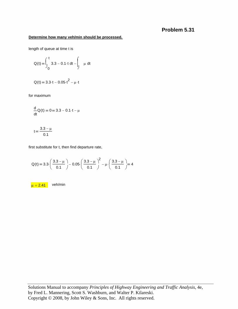
Solutions Manual to accompany Principles of Highway Engineering and Traffic Analysis, 4e, by Fred L. Mannering, Scott S. Washburn, and Walter P. Kilareski. Copyright © 2008, by John Wiley & Sons, Inc. All rights reserved.
Problem 5.31Determine how many veh/min should be processed.
length of queue at time t is
Q t( )0
tt3.3 0.1 t⋅−
⌠⎮⌡
d tμ⌠⎮⎮⌡
d−
Q t( ) 3.3 t⋅ 0.05 t2⋅− μ t⋅−
for maximum
tQ t( )d
d0 3.3 0.1 t⋅− μ−
t3.3 μ−
0.1
first substitute for t, then find departure rate,
Q t( ) 3.33.3 μ−
0.1⎛⎜⎝
⎞⎟⎠
⋅ 0.053.3 μ−
0.1⎛⎜⎝
⎞⎟⎠
2⋅− μ
3.3 μ−
0.1⎛⎜⎝
⎞⎟⎠
⋅− 4
μ 2.41= veh/min
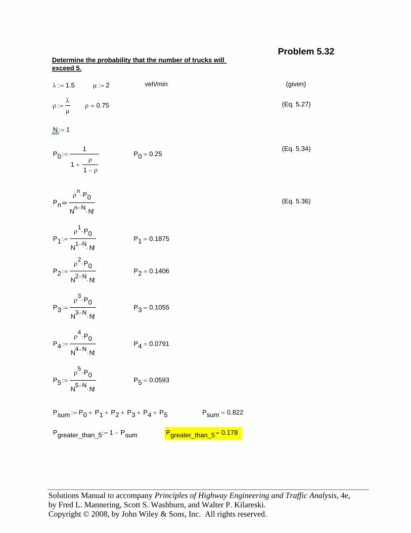
Solutions Manual to accompany Principles of Highway Engineering and Traffic Analysis, 4e, by Fred L. Mannering, Scott S. Washburn, and Walter P. Kilareski. Copyright © 2008, by John Wiley & Sons, Inc. All rights reserved.
Problem 5.32Determine the probability that the number of trucks will exceed 5.
λ 1.5:= μ 2:= veh/min (given)
ρλ
μ:= ρ 0.75= (Eq. 5.27)
N 1:=
(Eq. 5.34)P0
1
1ρ
1 ρ−+
:= P0 0.25=
Pnρ
n P0⋅
Nn N− N!⋅
(Eq. 5.36)
P1ρ
1 P0⋅
N1 N− N!⋅:= P1 0.1875=
P2ρ
2 P0⋅
N2 N− N!⋅:= P2 0.1406=
P3ρ
3 P0⋅
N3 N− N!⋅:= P3 0.1055=
P4ρ
4 P0⋅
N4 N− N!⋅:= P4 0.0791=
P5ρ
5 P0⋅
N5 N− N!⋅:= P5 0.0593=
Psum P0 P1+ P2+ P3+ P4+ P5+:= Psum 0.822=
Pgreater_than_5 1 Psum−:= Pgreater_than_5 0.178=
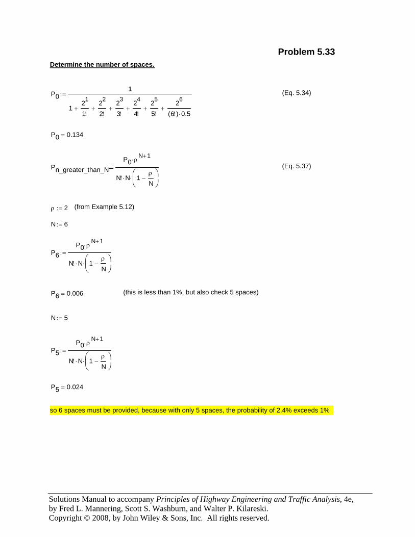
Solutions Manual to accompany Principles of Highway Engineering and Traffic Analysis, 4e, by Fred L. Mannering, Scott S. Washburn, and Walter P. Kilareski. Copyright © 2008, by John Wiley & Sons, Inc. All rights reserved.
so 6 spaces must be provided, because with only 5 spaces, the probability of 2.4% exceeds 1%
P5 0.024=
P5P0 ρ
N 1+⋅
N! N⋅ 1ρ
N−
⎛⎜⎝
⎞⎟⎠
⋅
:=
N 5:=
(this is less than 1%, but also check 5 spaces)P6 0.006=
P6P0 ρ
N 1+⋅
N! N⋅ 1ρ
N−
⎛⎜⎝
⎞⎟⎠
⋅
:=
N 6:=
(from Example 5.12)ρ 2:=
(Eq. 5.37)Pn_greater_than_NP0 ρ
N 1+⋅
N! N⋅ 1ρ
N−
⎛⎜⎝
⎞⎟⎠
⋅
P0 0.134=
(Eq. 5.34)P01
121
1!+
22
2!+
23
3!+
24
4!+
25
5!+
26
6!( ) 0.5⋅+
:=
Determine the number of spaces.
Problem 5.33
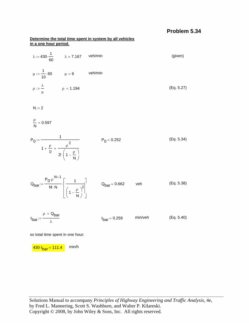
Solutions Manual to accompany Principles of Highway Engineering and Traffic Analysis, 4e, by Fred L. Mannering, Scott S. Washburn, and Walter P. Kilareski. Copyright © 2008, by John Wiley & Sons, Inc. All rights reserved.
min/h430 tbar⋅ 111.4=
so total time spent in one hour:
(Eq. 5.40)min/vehtbar 0.259=tbarρ Qbar+
λ:=
(Eq. 5.38)vehQbar 0.662=QbarP0 ρ
N 1+⋅
N! N⋅1
1ρ
N−
⎛⎜⎝
⎞⎟⎠
2⎡⎢⎢⎢⎣
⎤⎥⎥⎥⎦
⋅:=
(Eq. 5.34)P0 0.252=P01
1ρ
1!+
ρ2
2! 1ρ
N−
⎛⎜⎝
⎞⎟⎠
⋅
+
:=
ρ
N0.597=
N 2:=
(Eq. 5.27)ρ 1.194=ρλ
μ:=
veh/minμ 6=μ110
60⋅:=
(given)veh/minλ 7.167=λ 430160⋅:=
Determine the total time spent in system by all vehiclesin a one hour period.
Problem 5.34
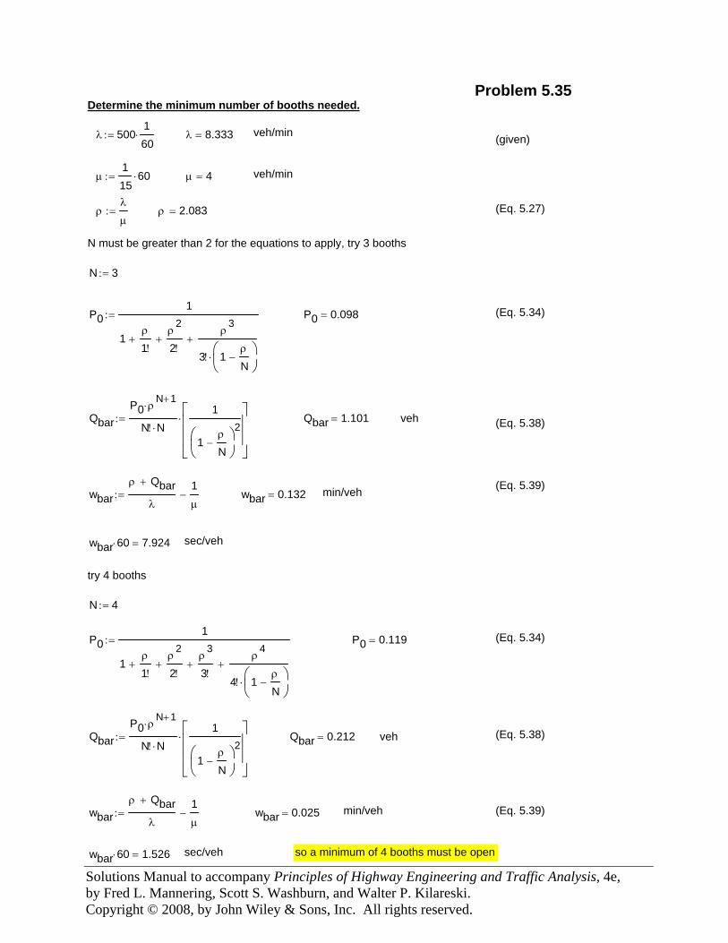
Solutions Manual to accompany Principles of Highway Engineering and Traffic Analysis, 4e, by Fred L. Mannering, Scott S. Washburn, and Walter P. Kilareski. Copyright © 2008, by John Wiley & Sons, Inc. All rights reserved.
wbarρ Qbar+
λ
1μ
−:= wbar 0.132= min/veh
wbar 60⋅ 7.924= sec/veh
try 4 booths
N 4:=
P01
1ρ
1!+
ρ2
2!+
ρ3
3!+
ρ4
4! 1ρ
N−
⎛⎜⎝
⎞⎟⎠
⋅
+
:= P0 0.119= (Eq. 5.34)
QbarP0 ρ
N 1+⋅
N! N⋅1
1ρ
N−
⎛⎜⎝
⎞⎟⎠
2⎡⎢⎢⎢⎣
⎤⎥⎥⎥⎦
⋅:= Qbar 0.212= veh (Eq. 5.38)
wbarρ Qbar+
λ
1μ
−:= wbar 0.025= min/veh (Eq. 5.39)
wbar 60⋅ 1.526= sec/veh so a minimum of 4 booths must be open
Problem 5.35Determine the minimum number of booths needed.
λ 500160⋅:= λ 8.333= veh/min (given)
μ115
60⋅:= μ 4= veh/min
ρλ
μ:= ρ 2.083= (Eq. 5.27)
N must be greater than 2 for the equations to apply, try 3 booths
N 3:=
P01
1ρ
1!+
ρ2
2!+
ρ3
3! 1ρ
N−
⎛⎜⎝
⎞⎟⎠
⋅
+
:= P0 0.098= (Eq. 5.34)
QbarP0 ρ
N 1+⋅
N! N⋅1
1ρ
N−
⎛⎜⎝
⎞⎟⎠
2⎡⎢⎢⎢⎣
⎤⎥⎥⎥⎦
⋅:= Qbar 1.101= veh (Eq. 5.38)
(Eq. 5.39)
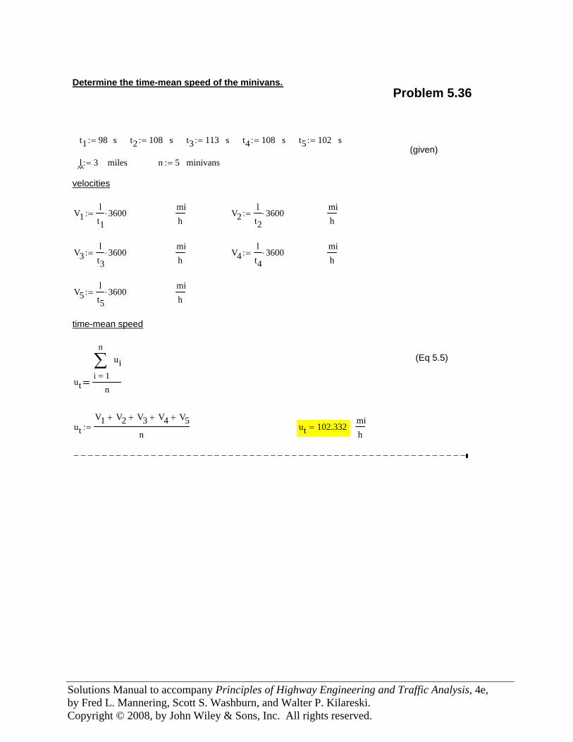
Solutions Manual to accompany Principles of Highway Engineering and Traffic Analysis, 4e, by Fred L. Mannering, Scott S. Washburn, and Walter P. Kilareski. Copyright © 2008, by John Wiley & Sons, Inc. All rights reserved.
Determine the time-mean speed of the minivans.Problem 5.36
t1 98:= s t2 108:= s t3 113:= s t4 108:= s t5 102:= s(given)
l 3:= miles n 5:= minivans
velocities
V1lt1
3600⋅:=mih
V2lt2
3600⋅:=mih
V3lt3
3600⋅:=mih
V4lt4
3600⋅:=mih
V5lt5
3600⋅:=mih
time-mean speed
(Eq 5.5)
ut1
n
i
ui∑=
n
utV1 V2+ V3+ V4+ V5+
n:= ut 102.332=
mih
−−−−−−−−−−−−−−−−−−−−−−−−−−−−−−−−−−−−−−−−−−−−−−−−−−−−−−−−
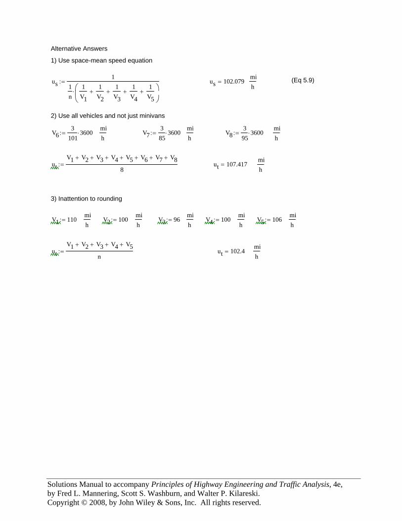
Solutions Manual to accompany Principles of Highway Engineering and Traffic Analysis, 4e, by Fred L. Mannering, Scott S. Washburn, and Walter P. Kilareski. Copyright © 2008, by John Wiley & Sons, Inc. All rights reserved.
−−−−−−−−−−−−−−−−−−−−−−−−−−−−−−−−−−−−−−−−−−−−−−−−−−−−−−Alternative Answers
1) Use space-mean speed equation
us1
1n
1V1
1V2
+1
V3+
1V4
+1
V5+⎛
⎜⎝
⎞⎟⎠
⋅
:= us 102.079=mih
(Eq 5.9)
2) Use all vehicles and not just minivans
V63
1013600⋅:=
mih
V7385
3600⋅:=mih
V8395
3600⋅:=mih
utV1 V2+ V3+ V4+ V5+ V6+ V7+ V8+
8:= ut 107.417=
mih
3) Inattention to rounding
V1 110:=mih
V2 100:=mih
V3 96:=mih
V4 100:=mih
V5 106:=mih
utV1 V2+ V3+ V4+ V5+
n:= ut 102.4=
mih
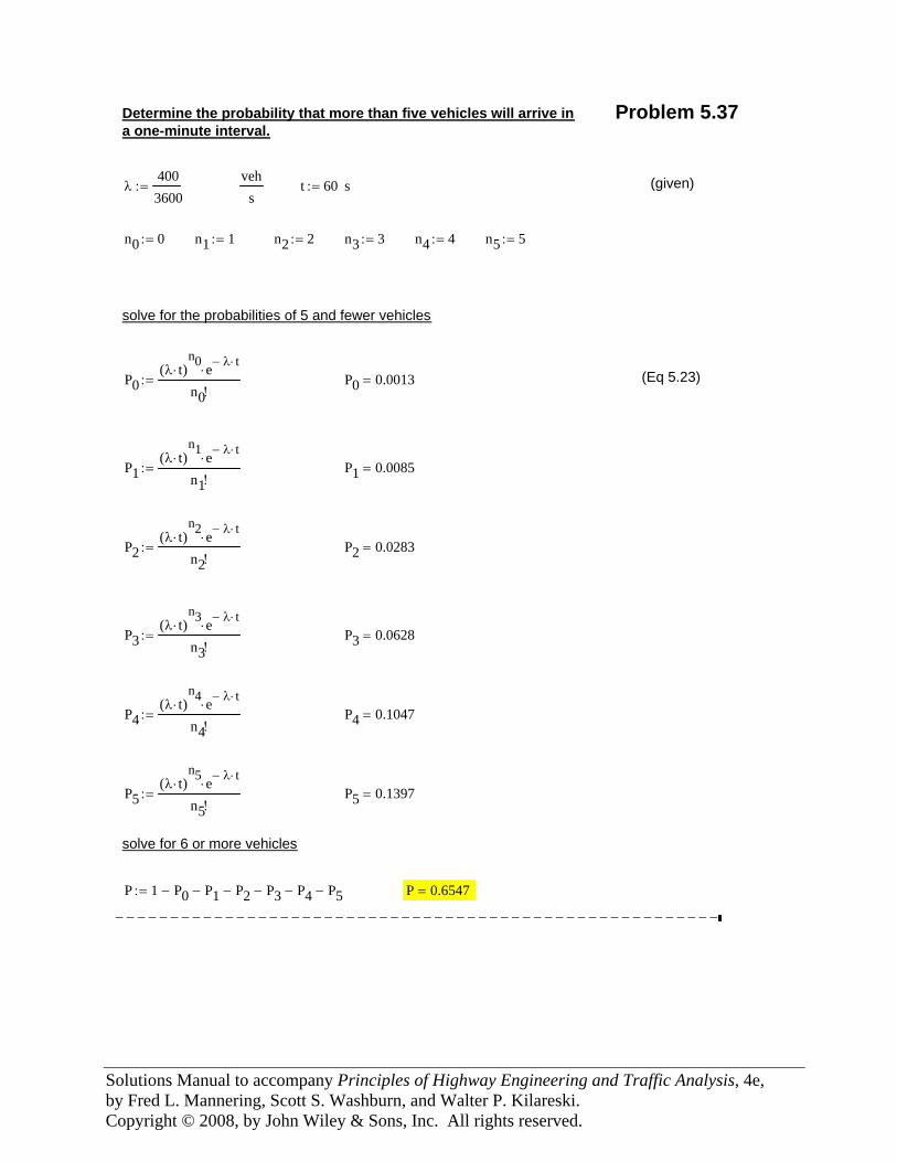
Solutions Manual to accompany Principles of Highway Engineering and Traffic Analysis, 4e, by Fred L. Mannering, Scott S. Washburn, and Walter P. Kilareski. Copyright © 2008, by John Wiley & Sons, Inc. All rights reserved.
Determine the probability that more than five vehicles will arrive ina one-minute interval.
Problem 5.37
λ4003600
:=veh
st 60:= s (given)
n0 0:= n1 1:= n2 2:= n3 3:= n4 4:= n5 5:=
solve for the probabilities of 5 and fewer vehicles
P0λ t⋅( )
n0 e λ− t⋅⋅
n0!:= P0 0.0013= (Eq 5.23)
P1λ t⋅( )
n1 e λ− t⋅⋅
n1!:= P1 0.0085=
P2λ t⋅( )
n2 e λ− t⋅⋅
n2!:= P2 0.0283=
P3λ t⋅( )
n3 e λ− t⋅⋅
n3!:= P3 0.0628=
P4λ t⋅( )
n4 e λ− t⋅⋅
n4!:= P4 0.1047=
P5λ t⋅( )
n5 e λ− t⋅⋅
n5!:= P5 0.1397=
solve for 6 or more vehicles
P 1 P0− P1− P2− P3− P4− P5−:= P 0.6547=
−−−−−−−−−−−−−−−−−−−−−−−−−−−−−−−−−−−−−−−−−−−−−−−−−−−−−−−
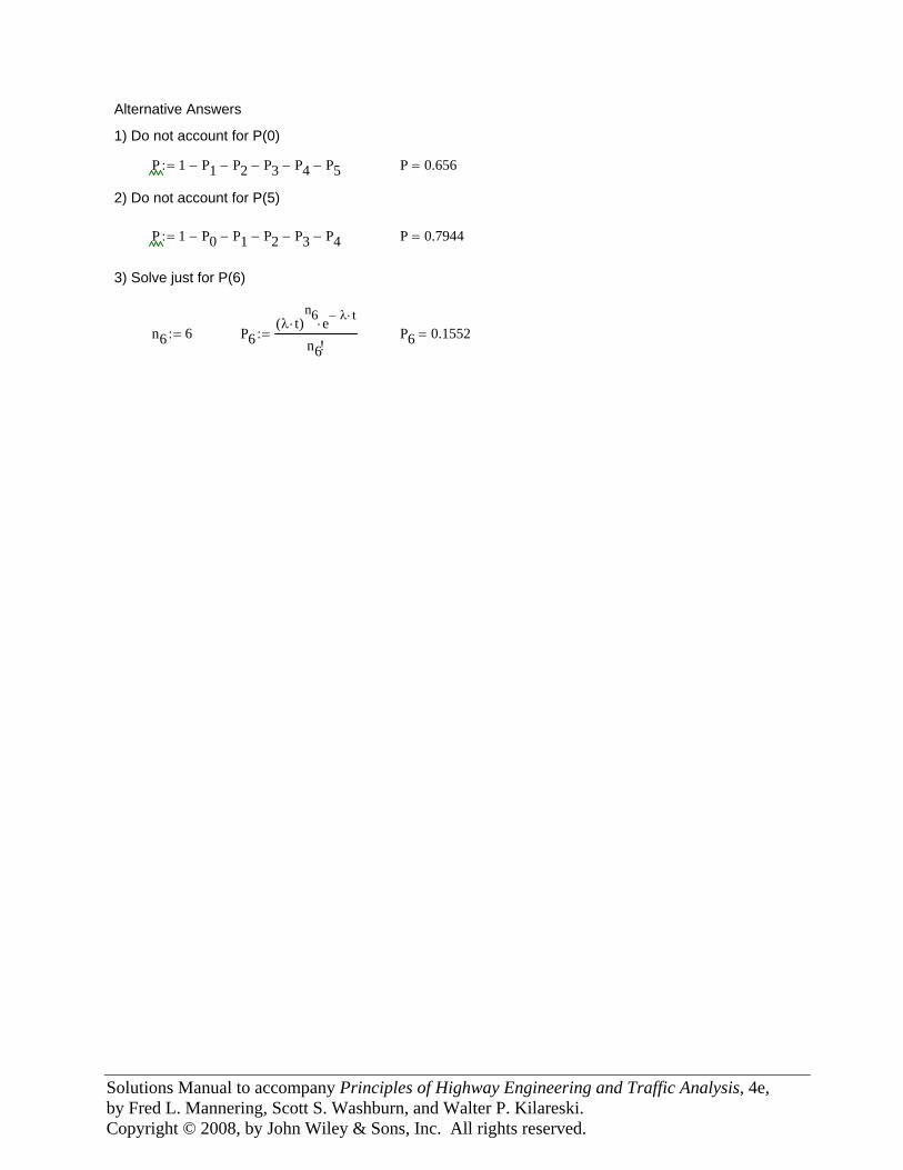
Solutions Manual to accompany Principles of Highway Engineering and Traffic Analysis, 4e, by Fred L. Mannering, Scott S. Washburn, and Walter P. Kilareski. Copyright © 2008, by John Wiley & Sons, Inc. All rights reserved.
−−−−−−−−−−−−−−−−−−−−−−−−−−−−−−−−−−Alternative Answers
1) Do not account for P(0)
P 1 P1− P2− P3− P4− P5−:= P 0.656=
2) Do not account for P(5)
P 1 P0− P1− P2− P3− P4−:= P 0.7944=
3) Solve just for P(6)
n6 6:= P6λ t⋅( )
n6 e λ− t⋅⋅
n6!:= P6 0.1552=
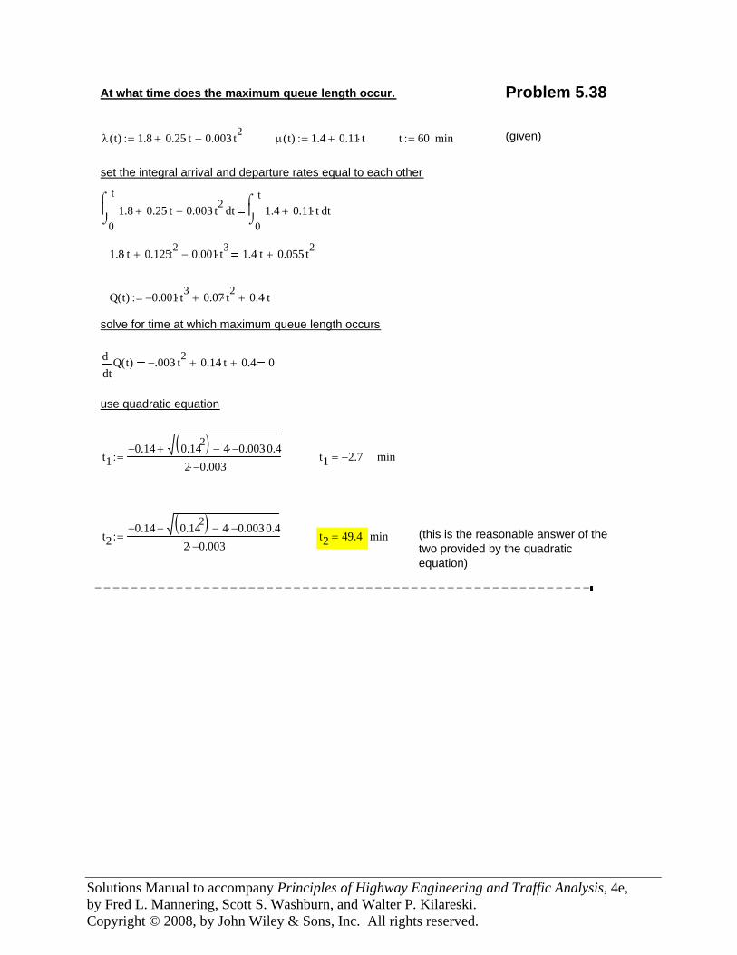
Solutions Manual to accompany Principles of Highway Engineering and Traffic Analysis, 4e, by Fred L. Mannering, Scott S. Washburn, and Walter P. Kilareski. Copyright © 2008, by John Wiley & Sons, Inc. All rights reserved.
At what time does the maximum queue length occur. Problem 5.38
λ t( ) 1.8 0.25 t⋅+ 0.003 t2⋅−:= μ t( ) 1.4 0.11 t⋅+:= t 60:= min (given)
set the integral arrival and departure rates equal to each other
0
t
t1.8 0.25 t⋅+ 0.003 t2⋅−⌠⎮⌡
d0
tt1.4 0.11 t⋅+
⌠⎮⌡
d
1.8 t⋅ 0.125t2+ 0.001 t3⋅− 1.4 t⋅ 0.055 t2⋅+
Q t( ) 0.001− t3⋅ 0.07 t2⋅+ 0.4 t⋅+:=
solve for time at which maximum queue length occurs
tQ t( )d
d.003− t2⋅ 0.14 t⋅+ 0.4+ 0
use quadratic equation
t10.14− 0.142( ) 4 0.003−⋅ 0.4⋅−+
2 0.003−⋅:= t1 2.7−= min
t20.14− 0.142( ) 4 0.003−⋅ 0.4⋅−−
2 0.003−⋅:= t2 49.4= min (this is the reasonable answer of the
two provided by the quadraticequation)
−−−−−−−−−−−−−−−−−−−−−−−−−−−−−−−−−−−−−−−−−−−−−−−−−−−−−−−
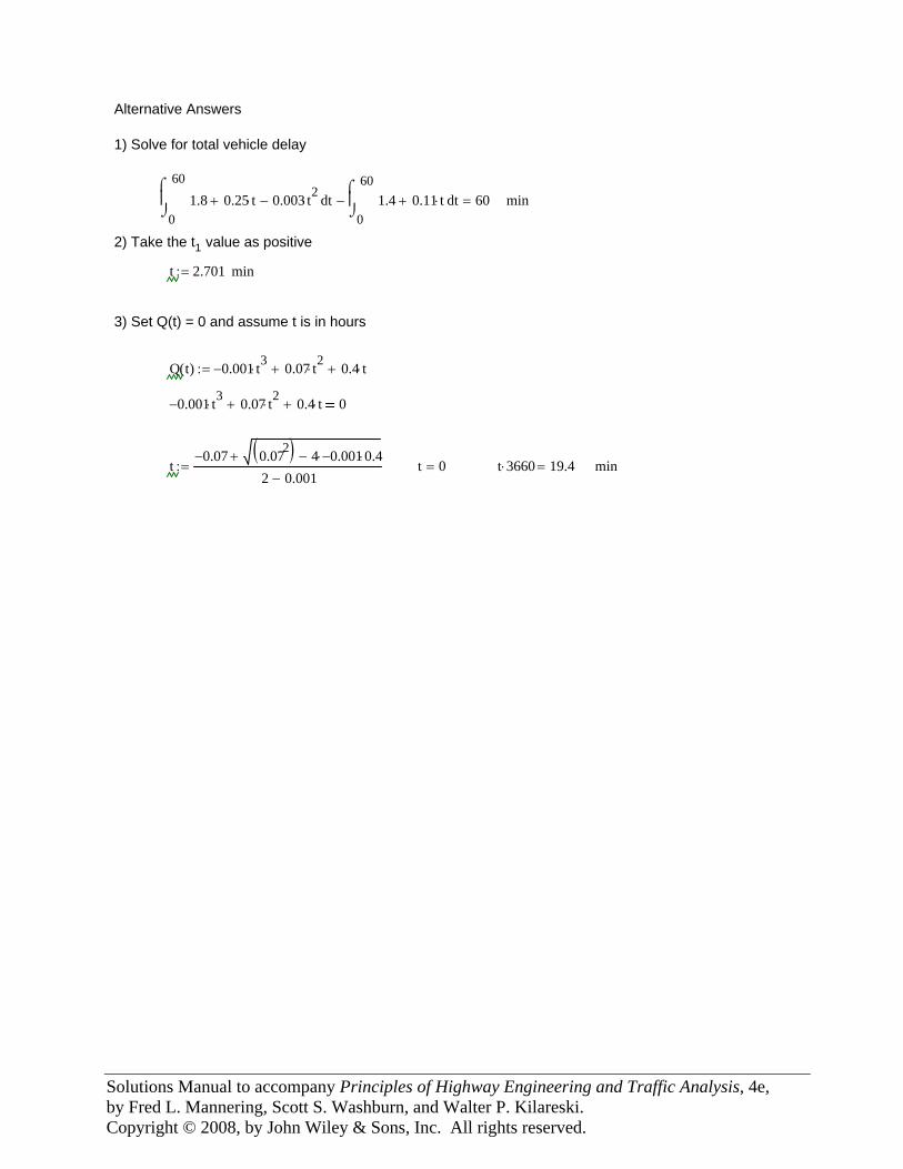
Solutions Manual to accompany Principles of Highway Engineering and Traffic Analysis, 4e, by Fred L. Mannering, Scott S. Washburn, and Walter P. Kilareski. Copyright © 2008, by John Wiley & Sons, Inc. All rights reserved.
−−−−−−−−−−−−−−−−−−−−−−−−−−−−−−−−−−−−−−−−−−−−−−−Alternative Answers
1) Solve for total vehicle delay
0
60
t1.8 0.25 t⋅+ 0.003 t2⋅−⌠⎮⌡
d0
60t1.4 0.11 t⋅+
⌠⎮⌡
d− 60= min
2) Take the t1 value as positive
t 2.701:= min
3) Set Q(t) = 0 and assume t is in hours
Q t( ) 0.001− t3⋅ 0.07 t2⋅+ 0.4 t⋅+:=
0.001− t3⋅ 0.07 t2⋅+ 0.4 t⋅+ 0
t0.07− 0.072( ) 4 0.001−⋅ 0.4⋅−+
2 0.001−:= t 0= t 3660⋅ 19.4= min
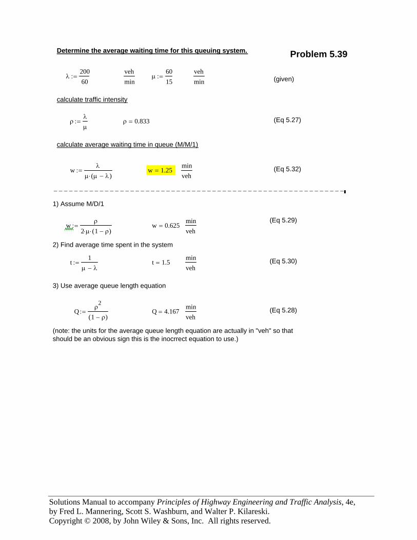
Solutions Manual to accompany Principles of Highway Engineering and Traffic Analysis, 4e, by Fred L. Mannering, Scott S. Washburn, and Walter P. Kilareski. Copyright © 2008, by John Wiley & Sons, Inc. All rights reserved.
Determine the average waiting time for this queuing system. Problem 5.39
λ20060
:=vehmin
μ6015
:=vehmin (given)
calculate traffic intensity
ρλ
μ:= ρ 0.833= (Eq 5.27)
calculate average waiting time in queue (M/M/1)
wλ
μ μ λ−( )⋅:= w 1.25=
minveh
(Eq 5.32)
−−−−−−−−−−−−−−−−−−−−−−−−−−−−−−−−−−−−−−−−−−−−−−−−−−−−−−−−−
1) Assume M/D/1
(Eq 5.29)w
ρ
2 μ⋅ 1 ρ−( )⋅:= w 0.625=
minveh
2) Find average time spent in the system
t1
μ λ−:= t 1.5=
minveh
(Eq 5.30)
3) Use average queue length equation
Qρ
2
1 ρ−( ):= Q 4.167=
minveh
(Eq 5.28)
(note: the units for the average queue length equation are actually in "veh" so thatshould be an obvious sign this is the inocrrect equation to use.)
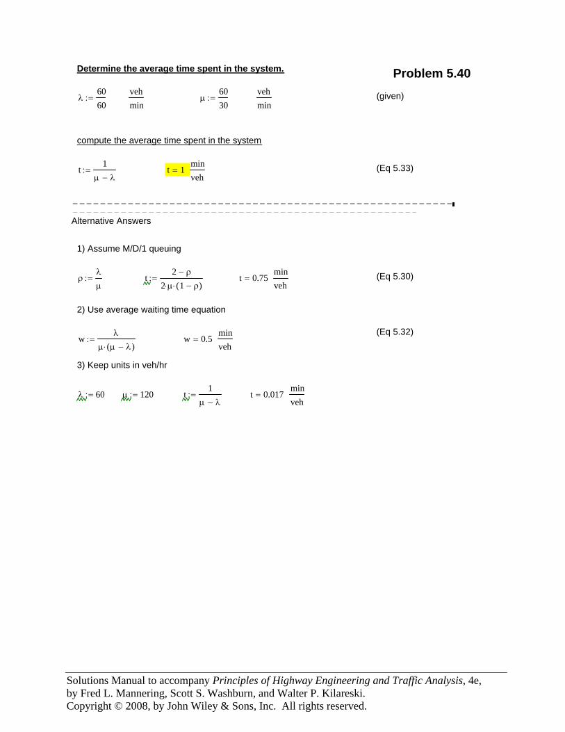
Solutions Manual to accompany Principles of Highway Engineering and Traffic Analysis, 4e, by Fred L. Mannering, Scott S. Washburn, and Walter P. Kilareski. Copyright © 2008, by John Wiley & Sons, Inc. All rights reserved.
Determine the average time spent in the system. Problem 5.40
λ6060
:=vehmin
μ6030
:=vehmin
(given)
compute the average time spent in the system
t1
μ λ−:= t 1=
minveh
(Eq 5.33)
−−−−−−−−−−−−−−−−−−−−−−−−−−−−−−−−−−−−−−−−−−−−−−−−−−−−−−−−−−−−−−−−−−−−−−−−−−−−−−−−−−−−−−−−−−−−−−−−−−−−−−−−−
Alternative Answers
1) Assume M/D/1 queuing
ρλ
μ:= t
2 ρ−
2 μ⋅ 1 ρ−( )⋅:= t 0.75=
minveh
(Eq 5.30)
2) Use average waiting time equation
(Eq 5.32)w
λ
μ μ λ−( )⋅:= w 0.5=
minveh
3) Keep units in veh/hr
λ 60:= μ 120:= t1
μ λ−:= t 0.017=
minveh
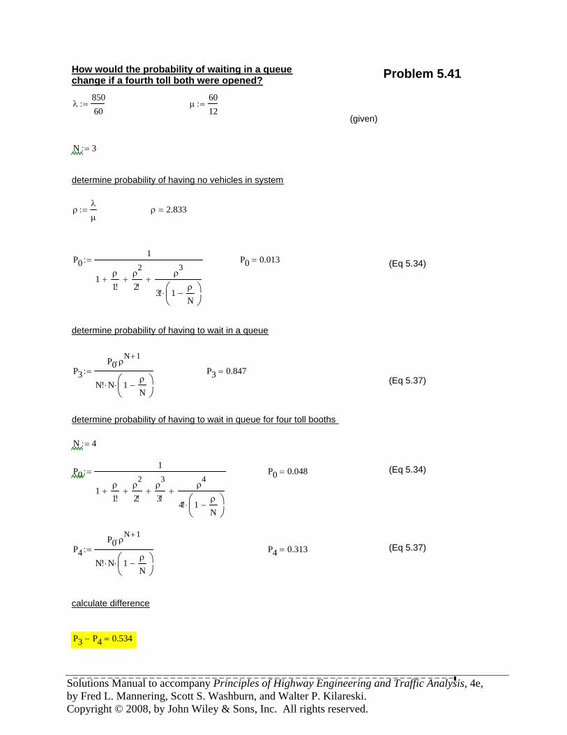
Solutions Manual to accompany Principles of Highway Engineering and Traffic Analysis, 4e, by Fred L. Mannering, Scott S. Washburn, and Walter P. Kilareski. Copyright © 2008, by John Wiley & Sons, Inc. All rights reserved.
How would the probability of waiting in a queuechange if a fourth toll both were opened? Problem 5.41
λ85060
:= μ6012
:=
(given)
N 3:=
determine probability of having no vehicles in system
ρλ
μ:= ρ 2.833=
P01
1ρ
1!+
ρ2
2!+
ρ3
3! 1ρ
N−⎛⎜
⎝⎞⎟⎠
⋅
+
:= P0 0.013= (Eq 5.34)
determine probability of having to wait in a queue
P3P0 ρ
N 1+⋅
N! N⋅ 1ρ
N−⎛⎜
⎝⎞⎟⎠
⋅
:= P3 0.847=(Eq 5.37)
determine probability of having to wait in queue for four toll booths
N 4:=
P01
1ρ
1!+
ρ2
2!+
ρ3
3!+
ρ4
4! 1ρ
N−⎛⎜
⎝⎞⎟⎠
⋅
+
:= P0 0.048= (Eq 5.34)
P4P0 ρ
N 1+⋅
N! N⋅ 1ρ
N−⎛⎜
⎝⎞⎟⎠
⋅
:= P4 0.313= (Eq 5.37)
calculate difference
P3 P4− 0.534=
−−−−−−−−−−−−−−−−−−−−−−−−−−−−−−−−−−−−−−−−−−−−−−−−−−−−−−−
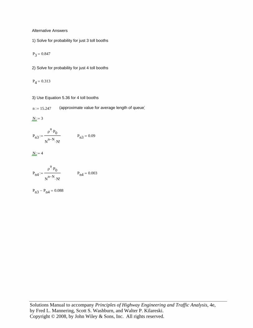
Solutions Manual to accompany Principles of Highway Engineering and Traffic Analysis, 4e, by Fred L. Mannering, Scott S. Washburn, and Walter P. Kilareski. Copyright © 2008, by John Wiley & Sons, Inc. All rights reserved.
Alternative Answers
1) Solve for probability for just 3 toll booths
P3 0.847=
2) Solve for probability for just 4 toll booths
P4 0.313=
3) Use Equation 5.36 for 4 toll booths
n 15.247:= (approximate value for average length of queue)
N 3:=
Pn3ρ
n P0⋅
Nn N− N!⋅:= Pn3 0.09=
N 4:=
Pn4ρ
n P0⋅
Nn N− N!⋅:= Pn4 0.003=
Pn3 Pn4− 0.088=
Solutions Manual to accompany
Principles of Highway Engineering and Traffic Analysis, 4e
By Fred L. Mannering, Scott S. Washburn, and Walter P. Kilareski
Chapter 6 Highway Capacity and Level of Service
Analysis
U.S. Customary Units
Copyright © 2008, by John Wiley & Sons, Inc. All rights reserved.

Solutions Manual to accompany Principles of Highway Engineering and Traffic Analysis, 4e, by Fred L. Mannering, Scott S. Washburn, and Walter P. Kilareski. Copyright © 2008, by John Wiley & Sons, Inc. All rights reserved.
Preface The solutions to the fourth edition of Principles of Highway Engineering and Traffic Analysis were prepared with the Mathcad1 software program. You will notice several notation conventions that you may not be familiar with if you are not a Mathcad user. Most of these notation conventions are self-explanatory or easily understood. The most common Mathcad specific notations in these solutions relate to the equals sign. You will notice the equals sign being used in three different contexts, and Mathcad uses three different notations to distinguish between each of these contexts. The differences between these equals sign notations are explained as follows.
• The ‘:=’ (colon-equals) is an assignment operator, that is, the value of the variable or expression on the left side of ‘:=’is set equal to the value of the expression on the right side. For example, in the statement, L := 1234, the variable ‘L’ is assigned (i.e., set equal to) the value of 1234. Another example is x := y + z. In this case, x is assigned the value of y + z.
• The ‘==’ (bold equals) is used when the Mathcad function solver was used to find the value of a variable in the equation. For example, in the equation
, the == is used to tell Mathcad that the value of the expression on the left side needs to equal the value of the expression on the right side. Thus, the Mathcad solver can be employed to find a value for the variable ‘t’ that satisfies this relationship. This particular example is from a problem where the function for arrivals at some time ‘t’ is set equal to the function for departures at some time ‘t’ to find the time to queue clearance.
• The ‘=’ (standard equals) is used for a simple numeric evaluation. For example, referring to the x := y + z assignment used previously, if the value of y was 10 [either by assignment (with :=), or the result of an equation solution (through the use of ==) and the value of z was 15, then the expression ‘x =’ would yield 25. Another example would be as follows: s := 1800/3600, with s = 0.5. That is, ‘s’ was assigned the value of 1800 divided by 3600 (using :=), which equals 0.5 (as given by using =).
Another symbol you will see frequently is ‘→’. In these solutions, it is used to perform an evaluation of an assignment expression in a single statement. For example, in the following
statement, , Q(t) is assigned the value of Arrivals(t) – Departures(t), and this evaluates to 2.2t – 0.10t2. Finally, to assist in quickly identifying the final answer, or answers, for what is being asked in the problem statement, yellow highlighting has been used (which will print as light gray). 1 www.mathcad.com
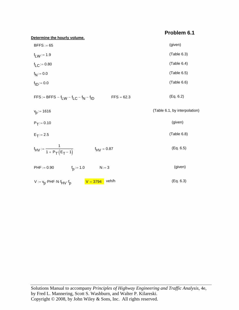
Solutions Manual to accompany Principles of Highway Engineering and Traffic Analysis, 4e, by Fred L. Mannering, Scott S. Washburn, and Walter P. Kilareski. Copyright © 2008, by John Wiley & Sons, Inc. All rights reserved.
(Eq. 6.3)veh/h V 3794=V vp PHF⋅ N⋅ fHV⋅ fp⋅:=
(given)N 3:=fp 1.0:=PHF 0.90:=
(Eq. 6.5)fHV 0.87=fHV1
1 PT ET 1−( )⋅+:=
(Table 6.8)ET 2.5:=
(given)PT 0.10:=
(Table 6.1, by interpolation)vp 1616:=
(Eq. 6.2)FFS 62.3=FFS BFFS fLW− fLC− fN− fID−:=
(Table 6.6)fID 0.0:=
(Table 6.5)fN 0.0:=
(Table 6.4)fLC 0.80:=
(Table 6.3)fLW 1.9:=
(given)BFFS 65:=
Determine the hourly volume.Problem 6.1
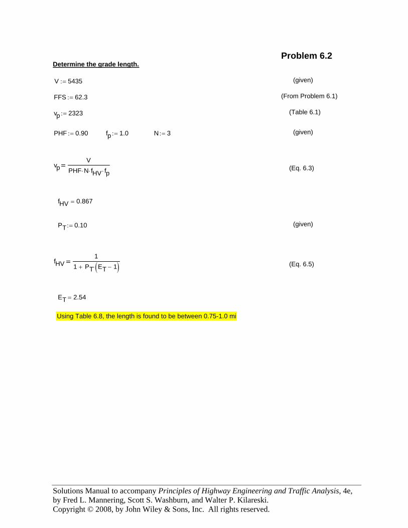
Solutions Manual to accompany Principles of Highway Engineering and Traffic Analysis, 4e, by Fred L. Mannering, Scott S. Washburn, and Walter P. Kilareski. Copyright © 2008, by John Wiley & Sons, Inc. All rights reserved.
Using Table 6.8, the length is found to be between 0.75-1.0 mi
ET 2.54=
(Eq. 6.5)fHV1
1 PT ET 1−( )⋅+
(given)PT 0.10:=
fHV 0.867=
(Eq. 6.3)vpV
PHF N⋅ fHV⋅ fp⋅
(given)N 3:=fp 1.0:=PHF 0.90:=
(Table 6.1) vp 2323:=
(From Problem 6.1)FFS 62.3:=
(given)V 5435:=
Determine the grade length.Problem 6.2
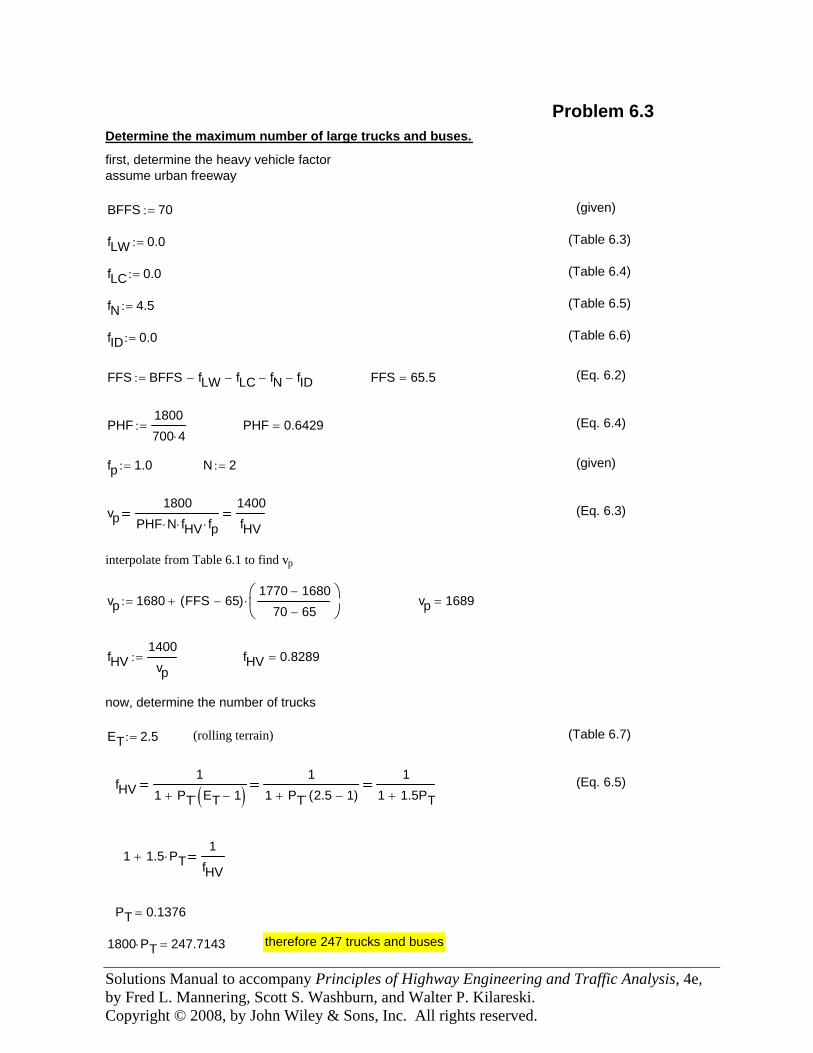
Solutions Manual to accompany Principles of Highway Engineering and Traffic Analysis, 4e, by Fred L. Mannering, Scott S. Washburn, and Walter P. Kilareski. Copyright © 2008, by John Wiley & Sons, Inc. All rights reserved.
(given)
vp1800
PHF N⋅ fHV⋅ fp⋅1400fHV
(Eq. 6.3)
interpolate from Table 6.1 to find vp
vp 1680 FFS 65−( )1770 1680−
70 65−⎛⎜⎝
⎞⎟⎠
⋅+:= vp 1689=
fHV1400
vp:= fHV 0.8289=
now, determine the number of trucks
ET 2.5:= (rolling terrain) (Table 6.7)
fHV1
1 PT ET 1−( )⋅+
11 PT 2.5 1−( )⋅+
11 1.5PT+
(Eq. 6.5)
1 1.5 PT⋅+1
fHV
PT 0.1376=
1800 PT⋅ 247.7143= therefore 247 trucks and buses
Problem 6.3 Determine the maximum number of large trucks and buses.
first, determine the heavy vehicle factorassume urban freeway
BFFS 70:= (given)
fLW 0.0:= (Table 6.3)
fLC 0.0:= (Table 6.4)
fN 4.5:= (Table 6.5)
fID 0.0:= (Table 6.6)
FFS BFFS fLW− fLC− fN− fID−:= FFS 65.5= (Eq. 6.2)
PHF1800700 4⋅
:= PHF 0.6429= (Eq. 6.4)
fp 1.0:= N 2:=
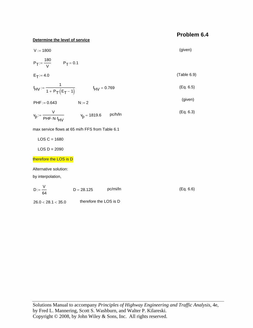
Solutions Manual to accompany Principles of Highway Engineering and Traffic Analysis, 4e, by Fred L. Mannering, Scott S. Washburn, and Walter P. Kilareski. Copyright © 2008, by John Wiley & Sons, Inc. All rights reserved.
therefore the LOS is D26.0 28.1< 35.0<
(Eq. 6.6)pc/mi/lnD 28.125=DV64
:=
by interpolation,
Alternative solution:
therefore the LOS is D
LOS C = 1680
LOS D = 2090
max service flows at 65 mi/h FFS from Table 6.1
pc/h/lnvp 1819.6=vpV
PHF N⋅ fHV⋅:=
(Eq. 6.3)
N 2:=PHF 0.643:=(given)
(Eq. 6.5)fHV 0.769=fHV1
1 PT ET 1−( )⋅+:=
(Table 6.9)ET 4.0:=
PT 0.1=PT180V
:=
(given)V 1800:=
Determine the level of serviceProblem 6.4
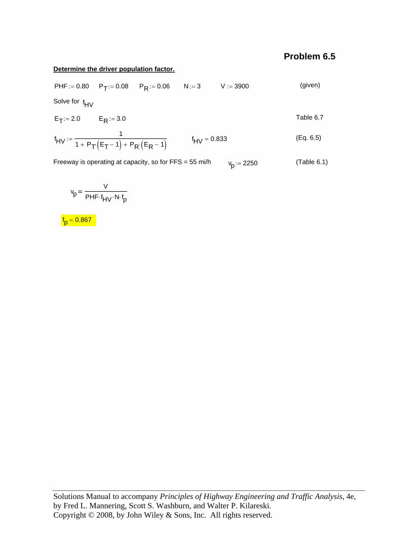
Solutions Manual to accompany Principles of Highway Engineering and Traffic Analysis, 4e, by Fred L. Mannering, Scott S. Washburn, and Walter P. Kilareski. Copyright © 2008, by John Wiley & Sons, Inc. All rights reserved.
fp 0.867=
vpV
PHF fHV⋅ N⋅ fp⋅
(Table 6.1)vp 2250:=Freeway is operating at capacity, so for FFS = 55 mi/h
(Eq. 6.5) fHV 0.833=fHV1
1 PT ET 1−( )⋅+ PR ER 1−( )⋅+:=
Table 6.7ER 3.0:=ET 2.0:=
fHVSolve for
(given)V 3900:=N 3:=PR 0.06:=PT 0.08:=PHF 0.80:=
Determine the driver population factor.
Problem 6.5
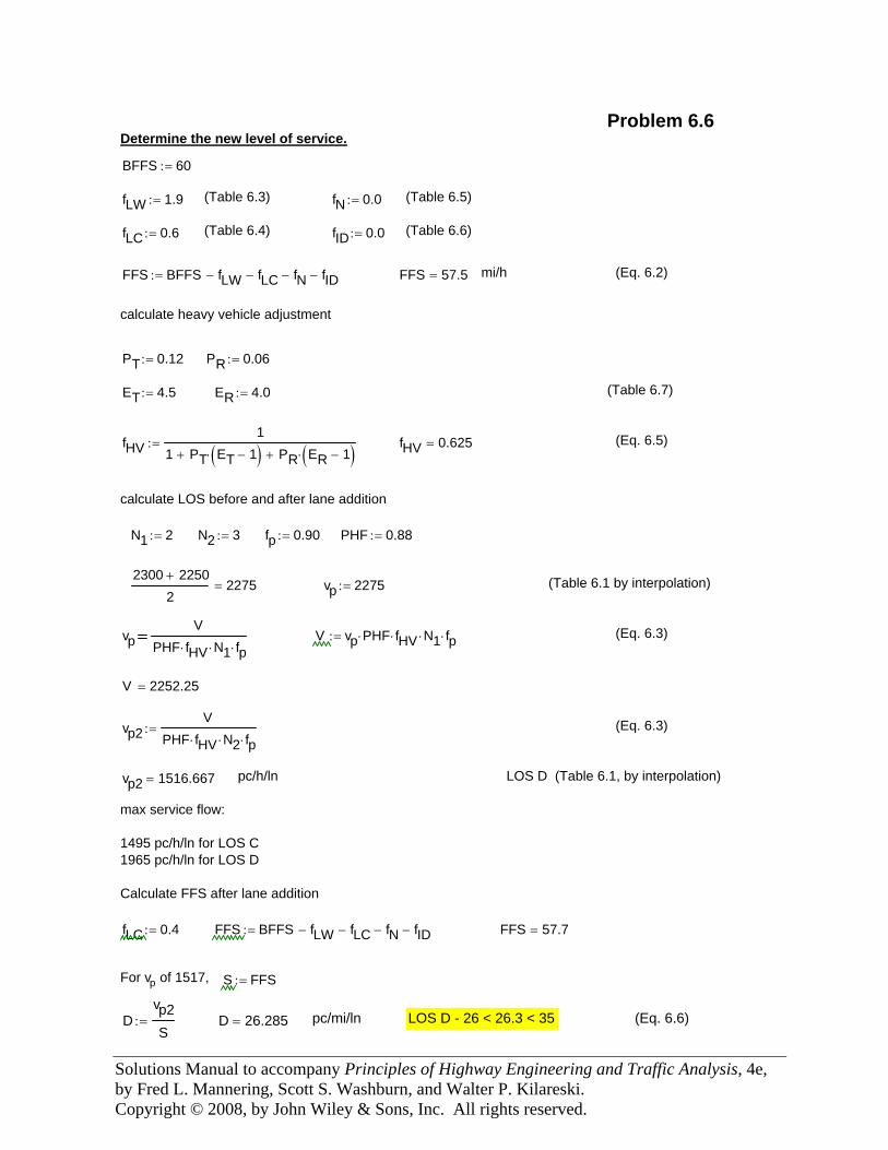
Solutions Manual to accompany Principles of Highway Engineering and Traffic Analysis, 4e, by Fred L. Mannering, Scott S. Washburn, and Walter P. Kilareski. Copyright © 2008, by John Wiley & Sons, Inc. All rights reserved.
Problem 6.6 Determine the new level of service.
BFFS 60:=
fLW 1.9:= (Table 6.3) fN 0.0:= (Table 6.5)
fLC 0.6:= (Table 6.4) fID 0.0:= (Table 6.6)
FFS BFFS fLW− fLC− fN− fID−:= FFS 57.5= mi/h (Eq. 6.2)
calculate heavy vehicle adjustment
PT 0.12:= PR 0.06:=
ET 4.5:= ER 4.0:= (Table 6.7)
fHV1
1 PT ET 1−( )⋅+ PR ER 1−( )⋅+:= fHV 0.625= (Eq. 6.5)
calculate LOS before and after lane addition
N1 2:= N2 3:= fp 0.90:= PHF 0.88:=
2300 2250+
22275= vp 2275:= (Table 6.1 by interpolation)
vpV
PHF fHV⋅ N1⋅ fp⋅V vp PHF⋅ fHV⋅ N1⋅ fp⋅:= (Eq. 6.3)
V 2252.25=
vp2V
PHF fHV⋅ N2⋅ fp⋅:= (Eq. 6.3)
vp2 1516.667= pc/h/ln LOS D (Table 6.1, by interpolation)
max service flow:
1495 pc/h/ln for LOS C1965 pc/h/ln for LOS D
Calculate FFS after lane addition
fLC 0.4:= FFS BFFS fLW− fLC− fN− fID−:= FFS 57.7=
For vp of 1517, S FFS:=
Dvp2S
:= D 26.285= pc/mi/ln LOS D - 26 < 26.3 < 35 (Eq. 6.6)
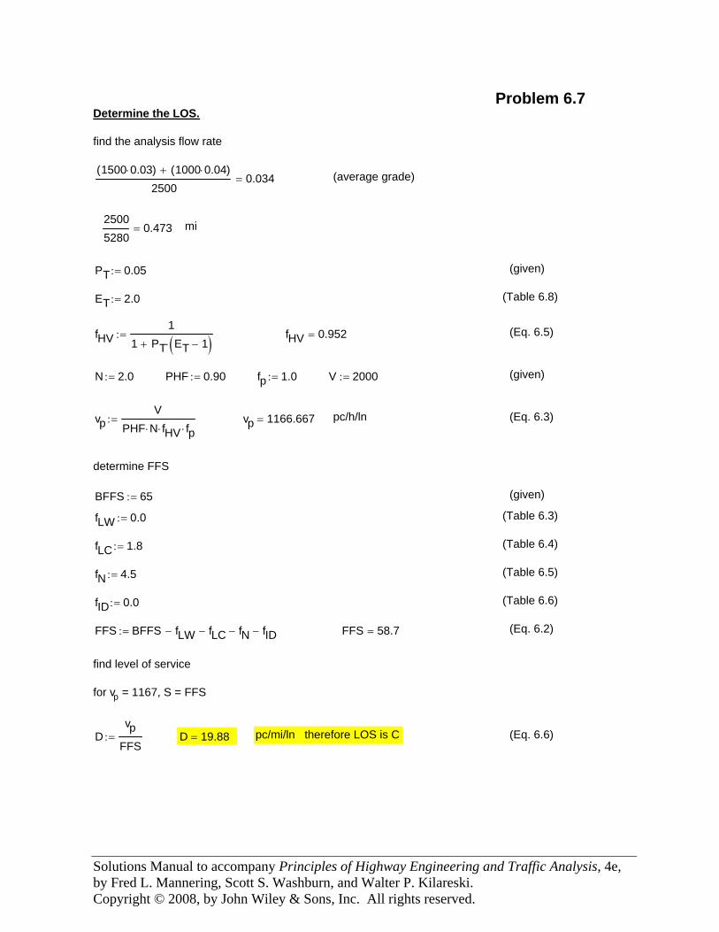
Solutions Manual to accompany Principles of Highway Engineering and Traffic Analysis, 4e, by Fred L. Mannering, Scott S. Washburn, and Walter P. Kilareski. Copyright © 2008, by John Wiley & Sons, Inc. All rights reserved.
(Eq. 6.3)
determine FFS
BFFS 65:= (given)
fLW 0.0:= (Table 6.3)
fLC 1.8:= (Table 6.4)
fN 4.5:= (Table 6.5)
fID 0.0:= (Table 6.6)
FFS BFFS fLW− fLC− fN− fID−:= FFS 58.7= (Eq. 6.2)
find level of service
for vp = 1167, S = FFS
Dvp
FFS:= D 19.88= pc/mi/ln therefore LOS is C (Eq. 6.6)
Problem 6.7 Determine the LOS.
find the analysis flow rate
1500 0.03⋅( ) 1000 0.04⋅( )+
25000.034= (average grade)
25005280
0.473= mi
PT 0.05:= (given)
ET 2.0:= (Table 6.8)
fHV1
1 PT ET 1−( )⋅+:= fHV 0.952= (Eq. 6.5)
N 2.0:= PHF 0.90:= fp 1.0:= V 2000:= (given)
vpV
PHF N⋅ fHV⋅ fp⋅:= vp 1166.667= pc/h/ln
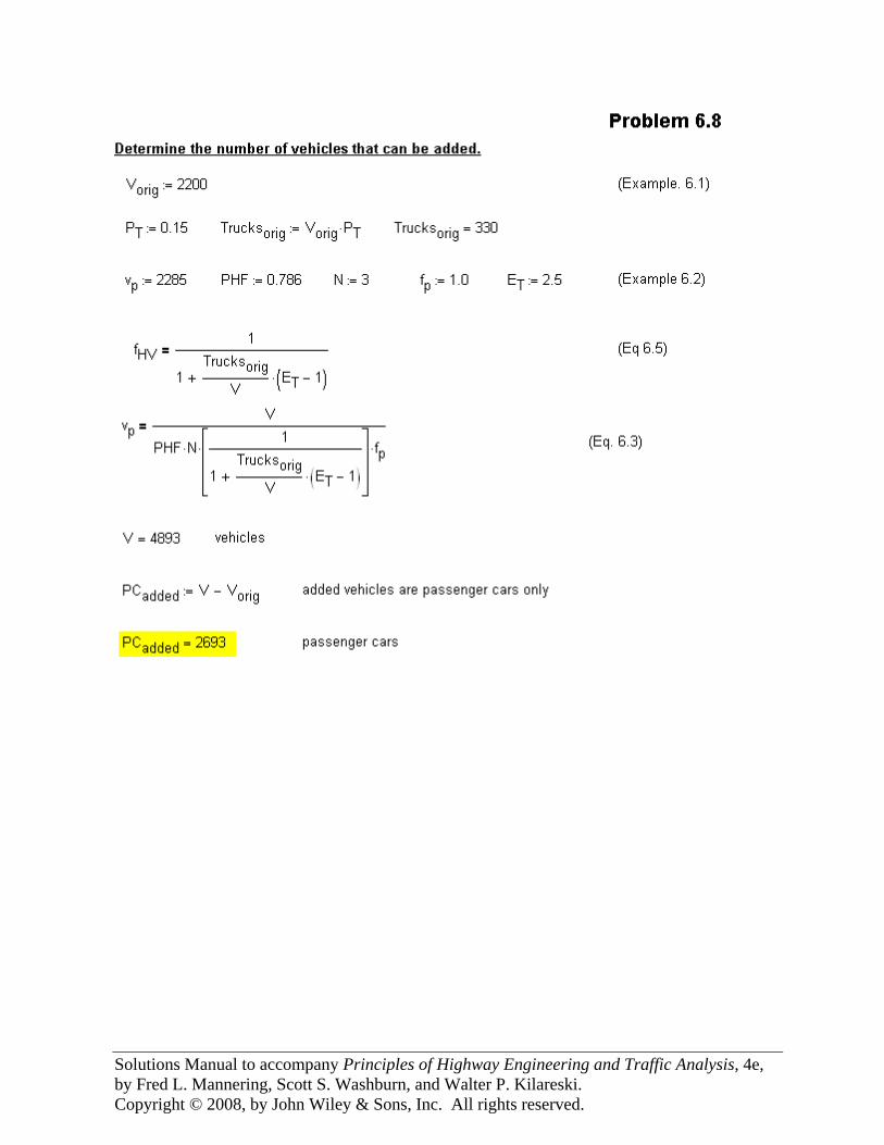
Solutions Manual to accompany Principles of Highway Engineering and Traffic Analysis, 4e, by Fred L. Mannering, Scott S. Washburn, and Walter P. Kilareski. Copyright © 2008, by John Wiley & Sons, Inc. All rights reserved.
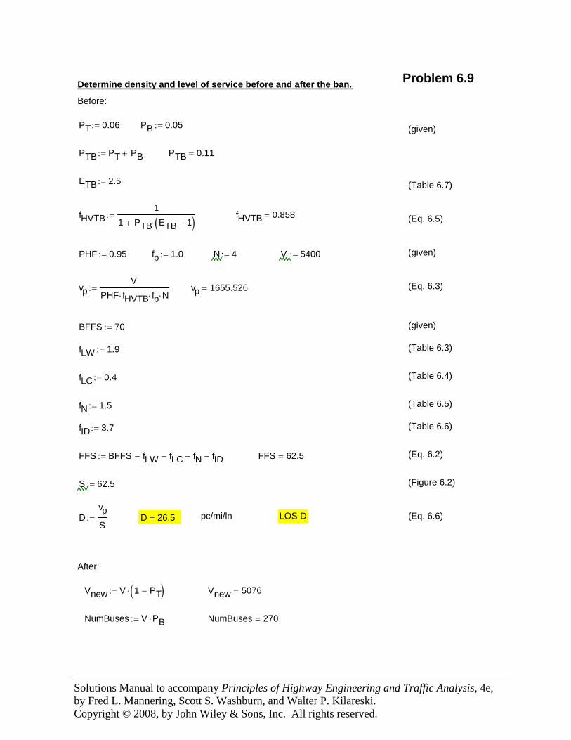
Solutions Manual to accompany Principles of Highway Engineering and Traffic Analysis, 4e, by Fred L. Mannering, Scott S. Washburn, and Walter P. Kilareski. Copyright © 2008, by John Wiley & Sons, Inc. All rights reserved.
Problem 6.9Determine density and level of service before and after the ban.
Before:
PT 0.06:= PB 0.05:= (given)
PTB PT PB+:= PTB 0.11=
ETB 2.5:= (Table 6.7)
fHVTB1
1 PTB ETB 1−( )⋅+:= fHVTB 0.858= (Eq. 6.5)
PHF 0.95:= fp 1.0:= N 4:= V 5400:= (given)
vpV
PHF fHVTB⋅ fp⋅ N⋅:= vp 1655.526= (Eq. 6.3)
BFFS 70:= (given)
fLW 1.9:= (Table 6.3)
fLC 0.4:= (Table 6.4)
fN 1.5:= (Table 6.5)
fID 3.7:= (Table 6.6)
FFS BFFS fLW− fLC− fN− fID−:= FFS 62.5= (Eq. 6.2)
S 62.5:= (Figure 6.2)
DvpS
:= D 26.5= pc/mi/ln LOS D (Eq. 6.6)
After:
Vnew V 1 PT−( )⋅:= Vnew 5076=
NumBuses V PB⋅:= NumBuses 270=
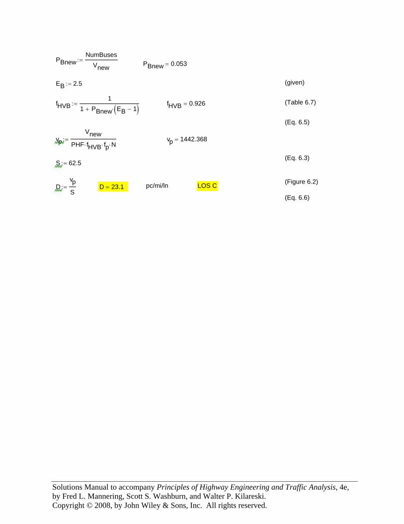
Solutions Manual to accompany Principles of Highway Engineering and Traffic Analysis, 4e, by Fred L. Mannering, Scott S. Washburn, and Walter P. Kilareski. Copyright © 2008, by John Wiley & Sons, Inc. All rights reserved.
PBnewNumBuses
Vnew:= PBnew 0.053=
EB 2.5:= (given)
fHVB1
1 PBnew EB 1−( )⋅+:= fHVB 0.926= (Table 6.7)
(Eq. 6.5)
vpVnew
PHF fHVB⋅ fp⋅ N⋅:= vp 1442.368=
(Eq. 6.3)S 62.5:=
(Figure 6.2)D
vpS
:= D 23.1= pc/mi/ln LOS C
(Eq. 6.6)
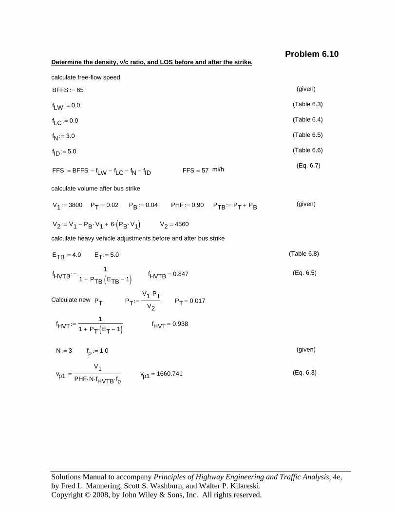
Solutions Manual to accompany Principles of Highway Engineering and Traffic Analysis, 4e, by Fred L. Mannering, Scott S. Washburn, and Walter P. Kilareski. Copyright © 2008, by John Wiley & Sons, Inc. All rights reserved.
(given)
V2 V1 PB V1⋅− 6 PB V1⋅( )⋅+:= V2 4560=
calculate heavy vehicle adjustments before and after bus strike
ETB 4.0:= ET 5.0:= (Table 6.8)
fHVTB1
1 PTB ETB 1−( )⋅+:= fHVTB 0.847= (Eq. 6.5)
Calculate new PT PTV1 PT⋅
V2:= PT 0.017=
fHVT1
1 PT ET 1−( )⋅+:= fHVT 0.938=
N 3:= fp 1.0:= (given)
vp1V1
PHF N⋅ fHVTB⋅ fp⋅:= vp1 1660.741= (Eq. 6.3)
Problem 6.10 Determine the density, v/c ratio, and LOS before and after the strike.
calculate free-flow speed
BFFS 65:= (given)
fLW 0.0:= (Table 6.3)
fLC 0.0:= (Table 6.4)
fN 3.0:= (Table 6.5)
fID 5.0:= (Table 6.6)
(Eq. 6.7)FFS BFFS fLW− fLC− fN− fID−:= FFS 57= mi/h
calculate volume after bus strike
V1 3800:= PT 0.02:= PB 0.04:= PHF 0.90:= PTB PT PB+:=
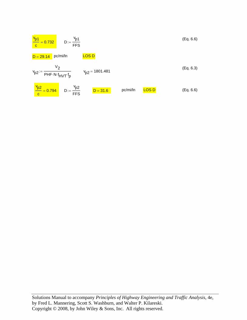
Solutions Manual to accompany Principles of Highway Engineering and Traffic Analysis, 4e, by Fred L. Mannering, Scott S. Washburn, and Walter P. Kilareski. Copyright © 2008, by John Wiley & Sons, Inc. All rights reserved.
(Eq. 6.6)vp1
c0.732= D
vp1FFS
:=
D 29.14= pc/mi/ln LOS D
(Eq. 6.3)vp2
V2PHF N⋅ fHVT⋅ fp⋅
:= vp2 1801.481=
vp2c
0.794= Dvp2FFS
:= D 31.6= pc/mi/ln LOS D (Eq. 6.6)
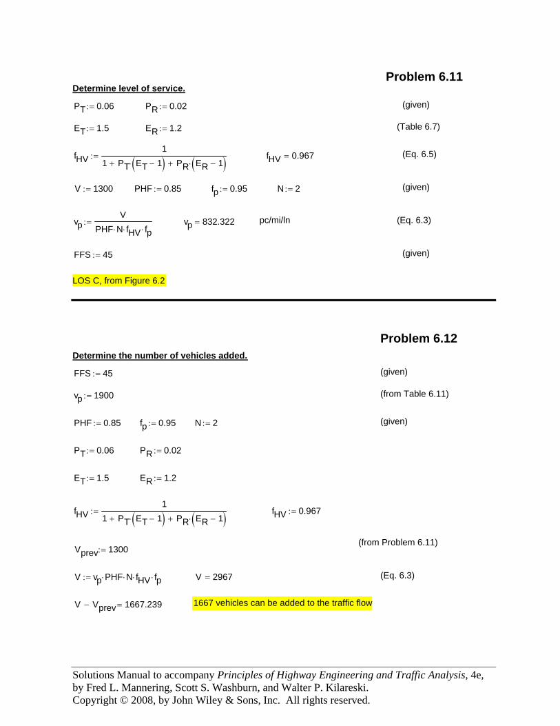
Solutions Manual to accompany Principles of Highway Engineering and Traffic Analysis, 4e, by Fred L. Mannering, Scott S. Washburn, and Walter P. Kilareski. Copyright © 2008, by John Wiley & Sons, Inc. All rights reserved.
LOS C, from Figure 6.2
(given)FFS 45:=
(Eq. 6.3)pc/mi/lnvp 832.322=vpV
PHF N⋅ fHV⋅ fp⋅:=
(given)N 2:=fp 0.95:=PHF 0.85:=V 1300:=
(Eq. 6.5)fHV 0.967=fHV1
1 PT ET 1−( )⋅+ PR ER 1−( )⋅+:=
(Table 6.7)ER 1.2:=ET 1.5:=
(given)PR 0.02:=PT 0.06:=
Determine level of service.Problem 6.11
1667 vehicles can be added to the traffic flowV Vprev− 1667.239=
(Eq. 6.3)V 2967=V vp PHF⋅ N⋅ fHV⋅ fp⋅:=
Vprev 1300:=(from Problem 6.11)
fHV 0.967:=fHV1
1 PT ET 1−( )⋅+ PR ER 1−( )⋅+:=
ER 1.2:=ET 1.5:=
PR 0.02:=PT 0.06:=
(given)N 2:=fp 0.95:=PHF 0.85:=
(from Table 6.11)vp 1900:=
(given)FFS 45:=
Determine the number of vehicles added.
Problem 6.12
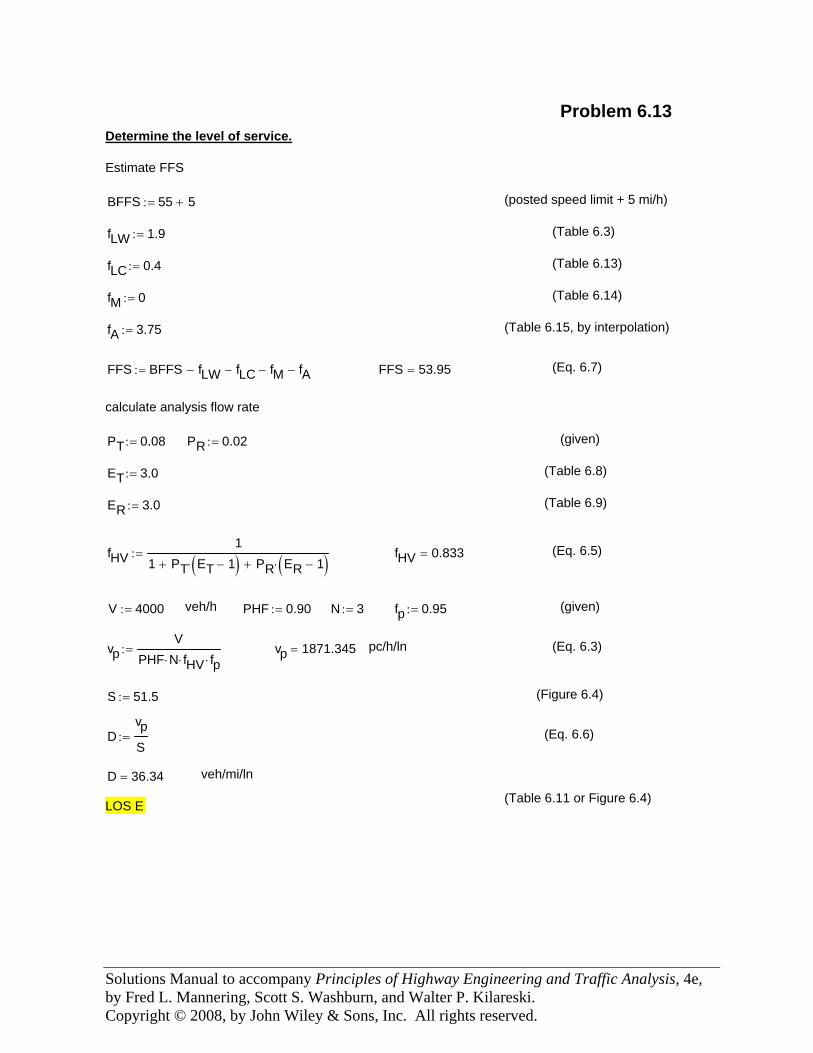
Solutions Manual to accompany Principles of Highway Engineering and Traffic Analysis, 4e, by Fred L. Mannering, Scott S. Washburn, and Walter P. Kilareski. Copyright © 2008, by John Wiley & Sons, Inc. All rights reserved.
(Table 6.9)
fHV1
1 PT ET 1−( )⋅+ PR ER 1−( )⋅+:= fHV 0.833= (Eq. 6.5)
V 4000:= veh/h PHF 0.90:= N 3:= fp 0.95:= (given)
vpV
PHF N⋅ fHV⋅ fp⋅:= vp 1871.345= pc/h/ln (Eq. 6.3)
S 51.5:= (Figure 6.4)
DvpS
:= (Eq. 6.6)
D 36.34= veh/mi/ln
(Table 6.11 or Figure 6.4) LOS E
Problem 6.13 Determine the level of service.
Estimate FFS
BFFS 55 5+:= (posted speed limit + 5 mi/h)
fLW 1.9:= (Table 6.3)
fLC 0.4:= (Table 6.13)
fM 0:= (Table 6.14)
fA 3.75:= (Table 6.15, by interpolation)
FFS BFFS fLW− fLC− fM− fA−:= FFS 53.95= (Eq. 6.7)
calculate analysis flow rate
PT 0.08:= PR 0.02:= (given)
ET 3.0:= (Table 6.8)
ER 3.0:=
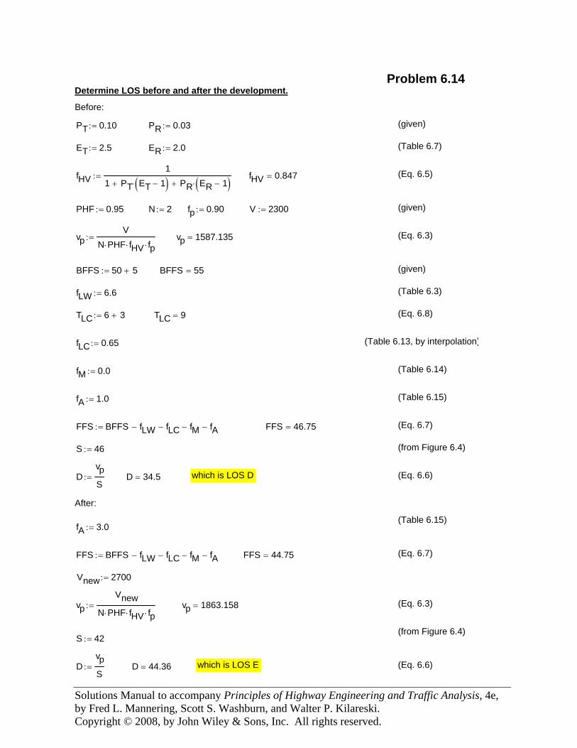
Solutions Manual to accompany Principles of Highway Engineering and Traffic Analysis, 4e, by Fred L. Mannering, Scott S. Washburn, and Walter P. Kilareski. Copyright © 2008, by John Wiley & Sons, Inc. All rights reserved.
fM 0.0:= (Table 6.14)
fA 1.0:= (Table 6.15)
FFS BFFS fLW− fLC− fM− fA−:= FFS 46.75= (Eq. 6.7)
S 46:= (from Figure 6.4)
DvpS
:= D 34.5= which is LOS D (Eq. 6.6)
After:
(Table 6.15)fA 3.0:=
FFS BFFS fLW− fLC− fM− fA−:= FFS 44.75= (Eq. 6.7)
Vnew 2700:=
vpVnew
N PHF⋅ fHV⋅ fp⋅:= vp 1863.158= (Eq. 6.3)
(from Figure 6.4)S 42:=
DvpS
:= D 44.36= which is LOS E (Eq. 6.6)
Problem 6.14 Determine LOS before and after the development.
Before:
PT 0.10:= PR 0.03:= (given)
ET 2.5:= ER 2.0:= (Table 6.7)
fHV1
1 PT ET 1−( )⋅+ PR ER 1−( )⋅+:= fHV 0.847= (Eq. 6.5)
PHF 0.95:= N 2:= fp 0.90:= V 2300:= (given)
vpV
N PHF⋅ fHV⋅ fp⋅:= vp 1587.135= (Eq. 6.3)
BFFS 50 5+:= BFFS 55= (given)
fLW 6.6:= (Table 6.3)
TLC 6 3+:= TLC 9= (Eq. 6.8)
fLC 0.65:= (Table 6.13, by interpolation)
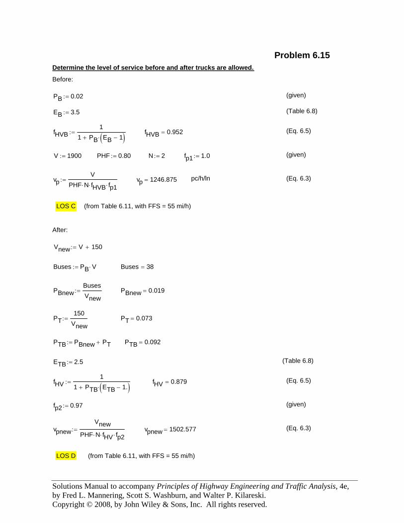
Solutions Manual to accompany Principles of Highway Engineering and Traffic Analysis, 4e, by Fred L. Mannering, Scott S. Washburn, and Walter P. Kilareski. Copyright © 2008, by John Wiley & Sons, Inc. All rights reserved.
Vnew V 150+:=
Buses PB V⋅:= Buses 38=
PBnewBusesVnew
:= PBnew 0.019=
PT150
Vnew:= PT 0.073=
PTB PBnew PT+:= PTB 0.092=
ETB 2.5:= (Table 6.8)
fHV1
1 PTB ETB 1.−( )⋅+:= fHV 0.879= (Eq. 6.5)
fp2 0.97:= (given)
vpnewVnew
PHF N⋅ fHV⋅ fp2⋅:= vpnew 1502.577= (Eq. 6.3)
LOS D (from Table 6.11, with FFS = 55 mi/h)
Problem 6.15 Determine the level of service before and after trucks are allowed.
Before:
PB 0.02:= (given)
EB 3.5:= (Table 6.8)
fHVB1
1 PB EB 1−( )⋅+:= fHVB 0.952= (Eq. 6.5)
V 1900:= PHF 0.80:= N 2:= fp1 1.0:= (given)
vpV
PHF N⋅ fHVB⋅ fp1⋅:= vp 1246.875= pc/h/ln (Eq. 6.3)
LOS C (from Table 6.11, with FFS = 55 mi/h)
After:
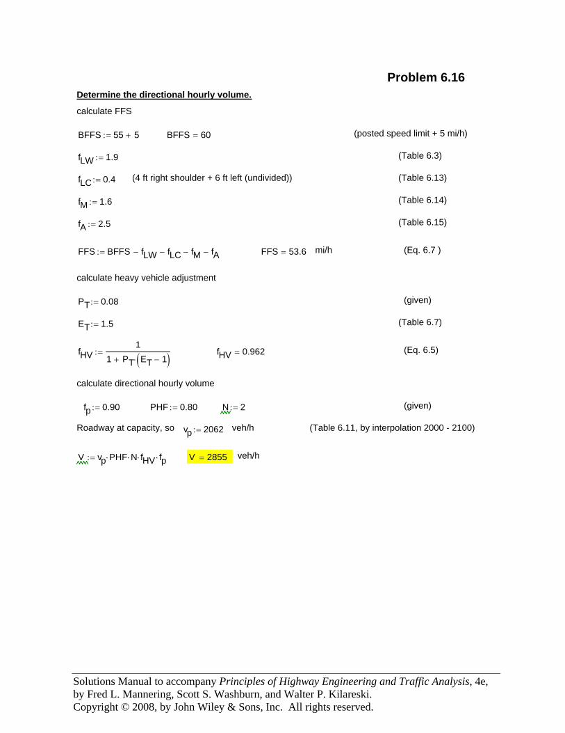
Solutions Manual to accompany Principles of Highway Engineering and Traffic Analysis, 4e, by Fred L. Mannering, Scott S. Washburn, and Walter P. Kilareski. Copyright © 2008, by John Wiley & Sons, Inc. All rights reserved.
Problem 6.16 Determine the directional hourly volume.
calculate FFS
BFFS 55 5+:= BFFS 60= (posted speed limit + 5 mi/h)
fLW 1.9:= (Table 6.3)
fLC 0.4:= (4 ft right shoulder + 6 ft left (undivided)) (Table 6.13)
fM 1.6:= (Table 6.14)
fA 2.5:= (Table 6.15)
FFS BFFS fLW− fLC− fM− fA−:= FFS 53.6= mi/h (Eq. 6.7 )
calculate heavy vehicle adjustment
PT 0.08:= (given)
ET 1.5:= (Table 6.7)
fHV1
1 PT ET 1−( )⋅+:= fHV 0.962= (Eq. 6.5)
calculate directional hourly volume
fp 0.90:= PHF 0.80:= N 2:= (given)
Roadway at capacity, so vp 2062:= veh/h (Table 6.11, by interpolation 2000 - 2100)
V vp PHF⋅ N⋅ fHV⋅ fp⋅:= V 2855= veh/h
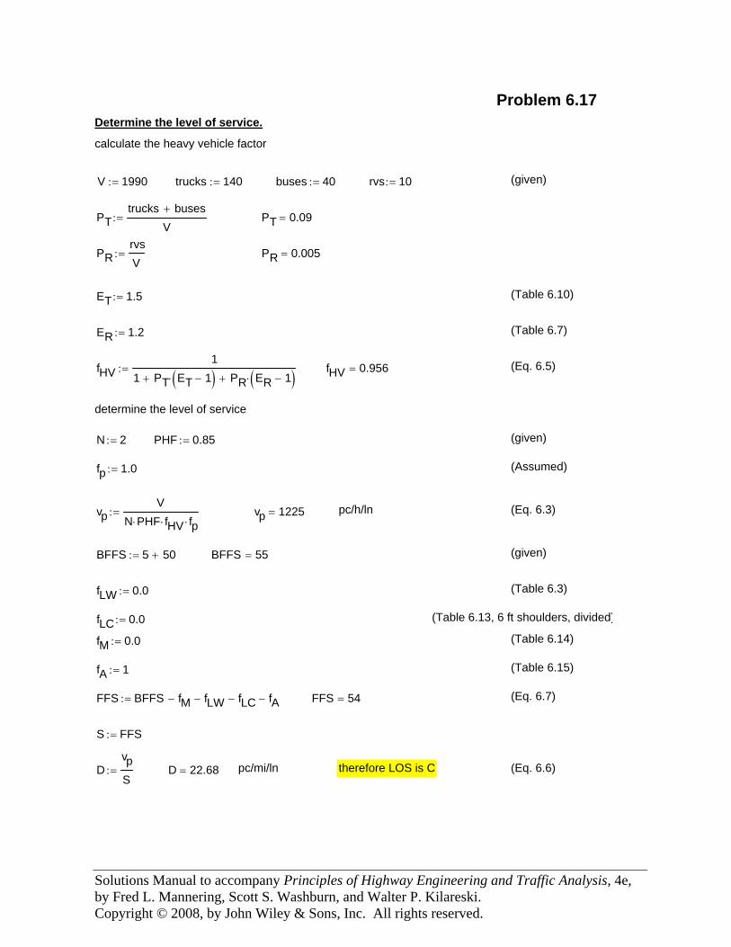
Solutions Manual to accompany Principles of Highway Engineering and Traffic Analysis, 4e, by Fred L. Mannering, Scott S. Washburn, and Walter P. Kilareski. Copyright © 2008, by John Wiley & Sons, Inc. All rights reserved.
vpV
N PHF⋅ fHV⋅ fp⋅:= vp 1225= pc/h/ln (Eq. 6.3)
BFFS 5 50+:= BFFS 55= (given)
fLW 0.0:= (Table 6.3)
fLC 0.0:= (Table 6.13, 6 ft shoulders, divided)
fM 0.0:= (Table 6.14)
fA 1:= (Table 6.15)
FFS BFFS fM− fLW− fLC− fA−:= FFS 54= (Eq. 6.7)
S FFS:=
DvpS
:= D 22.68= pc/mi/ln therefore LOS is C (Eq. 6.6)
Problem 6.17 Determine the level of service.
calculate the heavy vehicle factor
V 1990:= trucks 140:= buses 40:= rvs 10:= (given)
PTtrucks buses+
V:= PT 0.09=
PRrvsV
:= PR 0.005=
ET 1.5:= (Table 6.10)
ER 1.2:= (Table 6.7)
fHV1
1 PT ET 1−( )⋅+ PR ER 1−( )⋅+:= fHV 0.956= (Eq. 6.5)
determine the level of service
N 2:= PHF 0.85:= (given)
fp 1.0:= (Assumed)
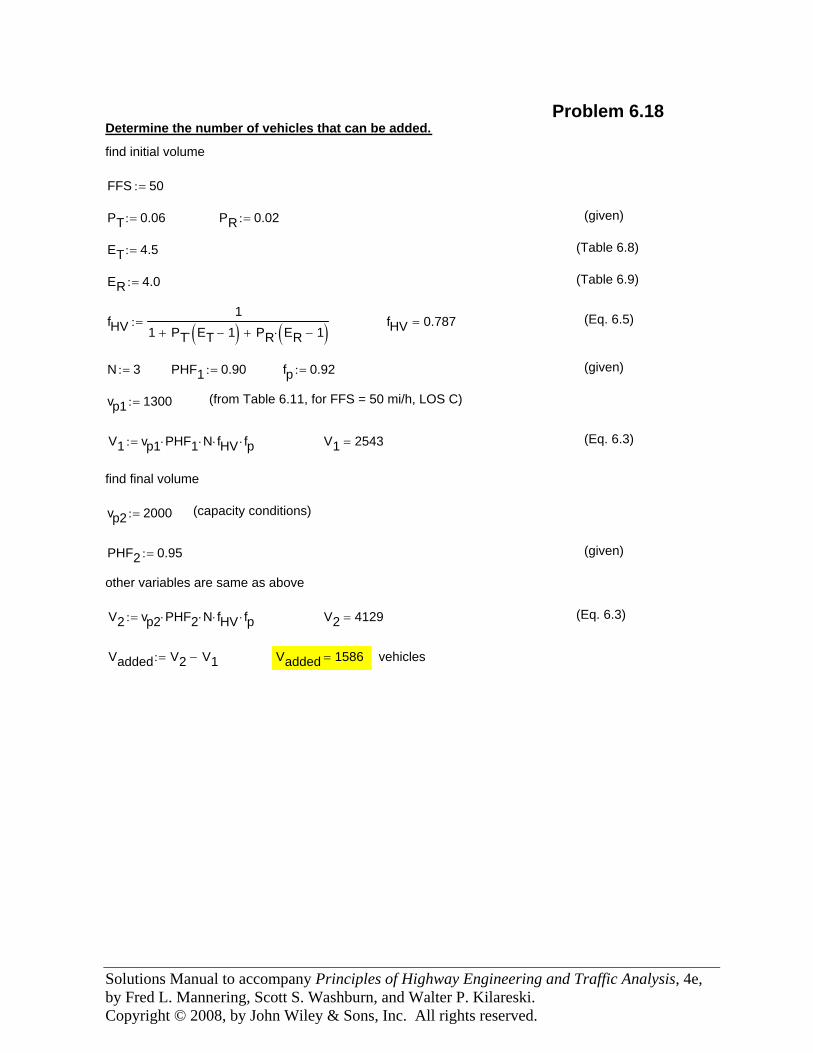
Solutions Manual to accompany Principles of Highway Engineering and Traffic Analysis, 4e, by Fred L. Mannering, Scott S. Washburn, and Walter P. Kilareski. Copyright © 2008, by John Wiley & Sons, Inc. All rights reserved.
vp1 1300:= (from Table 6.11, for FFS = 50 mi/h, LOS C)
V1 vp1 PHF1⋅ N⋅ fHV⋅ fp⋅:= V1 2543= (Eq. 6.3)
find final volume
vp2 2000:= (capacity conditions)
PHF2 0.95:= (given)
other variables are same as above
V2 vp2 PHF2⋅ N⋅ fHV⋅ fp⋅:= V2 4129= (Eq. 6.3)
Vadded V2 V1−:= Vadded 1586= vehicles
Problem 6.18 Determine the number of vehicles that can be added.
find initial volume
FFS 50:=
PT 0.06:= PR 0.02:= (given)
ET 4.5:= (Table 6.8)
ER 4.0:= (Table 6.9)
fHV1
1 PT ET 1−( )⋅+ PR ER 1−( )⋅+:= fHV 0.787= (Eq. 6.5)
N 3:= PHF1 0.90:= fp 0.92:= (given)
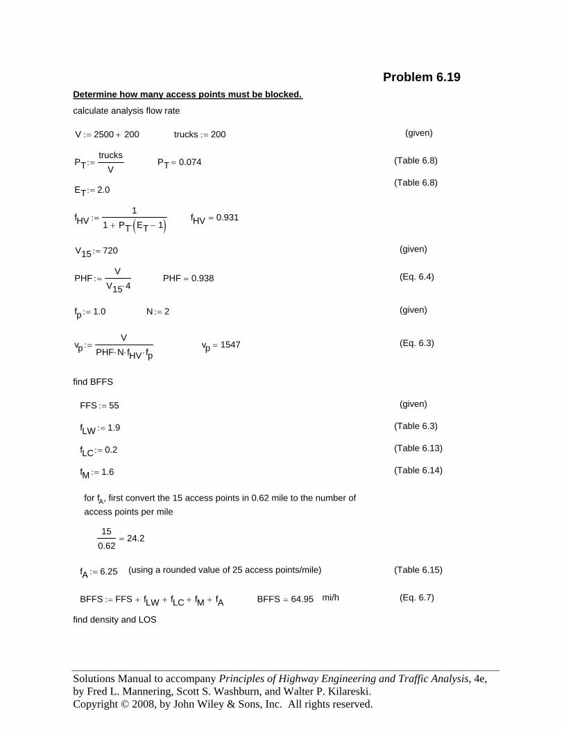
Solutions Manual to accompany Principles of Highway Engineering and Traffic Analysis, 4e, by Fred L. Mannering, Scott S. Washburn, and Walter P. Kilareski. Copyright © 2008, by John Wiley & Sons, Inc. All rights reserved.
vp 1547= (Eq. 6.3)
find BFFS
FFS 55:= (given)
fLW 1.9:= (Table 6.3)
fLC 0.2:= (Table 6.13)
fM 1.6:= (Table 6.14)
for fA, first convert the 15 access points in 0.62 mile to the number of access points per mile
150.62
24.2=
fA 6.25:= (using a rounded value of 25 access points/mile) (Table 6.15)
BFFS FFS fLW+ fLC+ fM+ fA+:= BFFS 64.95= mi/h (Eq. 6.7)
find density and LOS
Problem 6.19 Determine how many access points must be blocked.
calculate analysis flow rate
V 2500 200+:= trucks 200:= (given)
PTtrucks
V:= PT 0.074= (Table 6.8)
(Table 6.8)ET 2.0:=
fHV1
1 PT ET 1−( )⋅+:= fHV 0.931=
V15 720:= (given)
PHFV
V15 4⋅:= PHF 0.938= (Eq. 6.4)
fp 1.0:= N 2:= (given)
vpV
PHF N⋅ fHV⋅ fp⋅:=
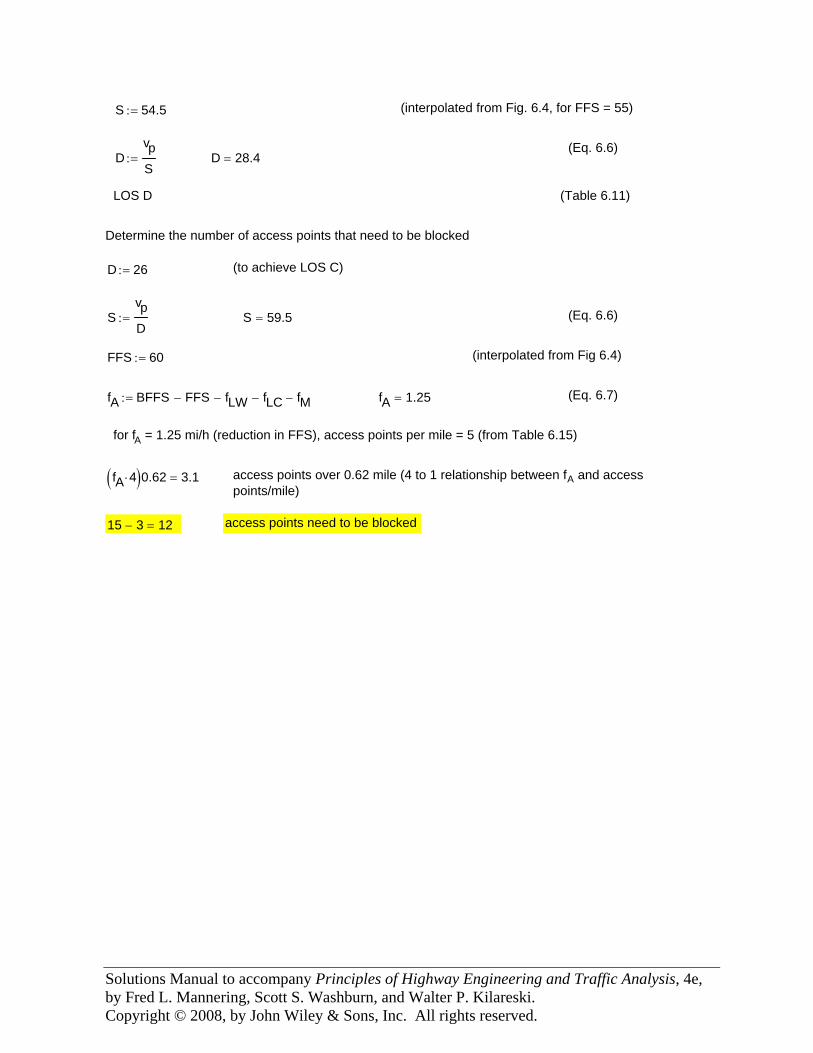
Solutions Manual to accompany Principles of Highway Engineering and Traffic Analysis, 4e, by Fred L. Mannering, Scott S. Washburn, and Walter P. Kilareski. Copyright © 2008, by John Wiley & Sons, Inc. All rights reserved.
access points need to be blocked15 3− 12=
access points over 0.62 mile (4 to 1 relationship between fA and access points/mile)
fA 4⋅( )0.62 3.1=
for fA = 1.25 mi/h (reduction in FFS), access points per mile = 5 (from Table 6.15)
(Eq. 6.7)fA 1.25=fA BFFS FFS− fLW− fLC− fM−:=
(interpolated from Fig 6.4)FFS 60:=
(Eq. 6.6)S 59.5=SvpD
:=
(to achieve LOS C)D 26:=
Determine the number of access points that need to be blocked
(Table 6.11)LOS D
D 28.4=DvpS
:=(Eq. 6.6)
(interpolated from Fig. 6.4, for FFS = 55)S 54.5:=
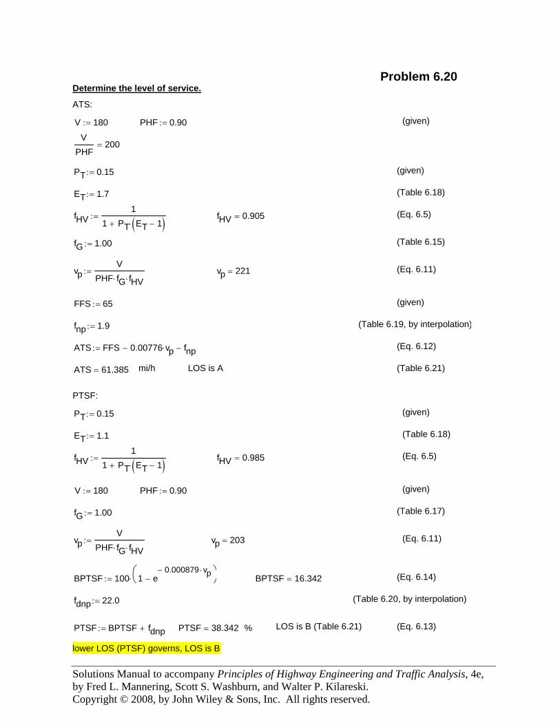
Solutions Manual to accompany Principles of Highway Engineering and Traffic Analysis, 4e, by Fred L. Mannering, Scott S. Washburn, and Walter P. Kilareski. Copyright © 2008, by John Wiley & Sons, Inc. All rights reserved.
(Table 6.21)
PTSF:
PT 0.15:= (given)
ET 1.1:= (Table 6.18)
fHV1
1 PT ET 1−( )⋅+:= fHV 0.985= (Eq. 6.5)
V 180:= PHF 0.90:= (given)
fG 1.00:= (Table 6.17)
vpV
PHF fG⋅ fHV⋅:= vp 203= (Eq. 6.11)
BPTSF 100 1 e0.000879− vp⋅
−⎛⎝
⎞⎠⋅:= BPTSF 16.342= (Eq. 6.14)
fdnp 22.0:= (Table 6.20, by interpolation)
PTSF BPTSF fdnp+:= PTSF 38.342= % LOS is B (Table 6.21) (Eq. 6.13)
lower LOS (PTSF) governs, LOS is B
Problem 6.20 Determine the level of service.
ATS:
V 180:= PHF 0.90:= (given)
VPHF
200=
PT 0.15:= (given)
ET 1.7:= (Table 6.18)
fHV1
1 PT ET 1−( )⋅+:= fHV 0.905= (Eq. 6.5)
fG 1.00:= (Table 6.15)
vpV
PHF fG⋅ fHV⋅:= vp 221= (Eq. 6.11)
FFS 65:= (given)
fnp 1.9:= (Table 6.19, by interpolation)
ATS FFS 0.00776 vp⋅− fnp−:= (Eq. 6.12)
ATS 61.385= mi/h LOS is A
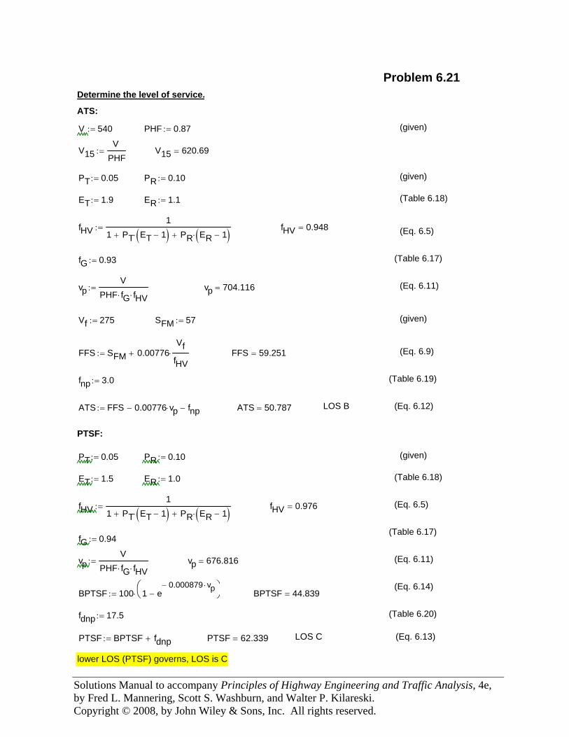
Solutions Manual to accompany Principles of Highway Engineering and Traffic Analysis, 4e, by Fred L. Mannering, Scott S. Washburn, and Walter P. Kilareski. Copyright © 2008, by John Wiley & Sons, Inc. All rights reserved.
Problem 6.21 Determine the level of service.
ATS:
V 540:= PHF 0.87:= (given)
V15V
PHF:= V15 620.69=
PT 0.05:= PR 0.10:= (given)
ET 1.9:= ER 1.1:= (Table 6.18)
fHV1
1 PT ET 1−( )⋅+ PR ER 1−( )⋅+:= fHV 0.948= (Eq. 6.5)
fG 0.93:= (Table 6.17)
vpV
PHF fG⋅ fHV⋅:= vp 704.116= (Eq. 6.11)
Vf 275:= SFM 57:= (given)
FFS SFM 0.00776Vf
fHV⋅+:= FFS 59.251= (Eq. 6.9)
fnp 3.0:= (Table 6.19)
ATS FFS 0.00776 vp⋅− fnp−:= ATS 50.787= LOS B (Eq. 6.12)
PTSF:
PT 0.05:= PR 0.10:= (given)
ET 1.5:= ER 1.0:= (Table 6.18)
fHV1
1 PT ET 1−( )⋅+ PR ER 1−( )⋅+:= fHV 0.976= (Eq. 6.5)
(Table 6.17)fG 0.94:=
vpV
PHF fG⋅ fHV⋅:= vp 676.816= (Eq. 6.11)
(Eq. 6.14)BPTSF 100 1 e
0.000879− vp⋅−
⎛⎝
⎞⎠⋅:= BPTSF 44.839=
fdnp 17.5:= (Table 6.20)
PTSF BPTSF fdnp+:= PTSF 62.339= LOS C (Eq. 6.13)
lower LOS (PTSF) governs, LOS is C
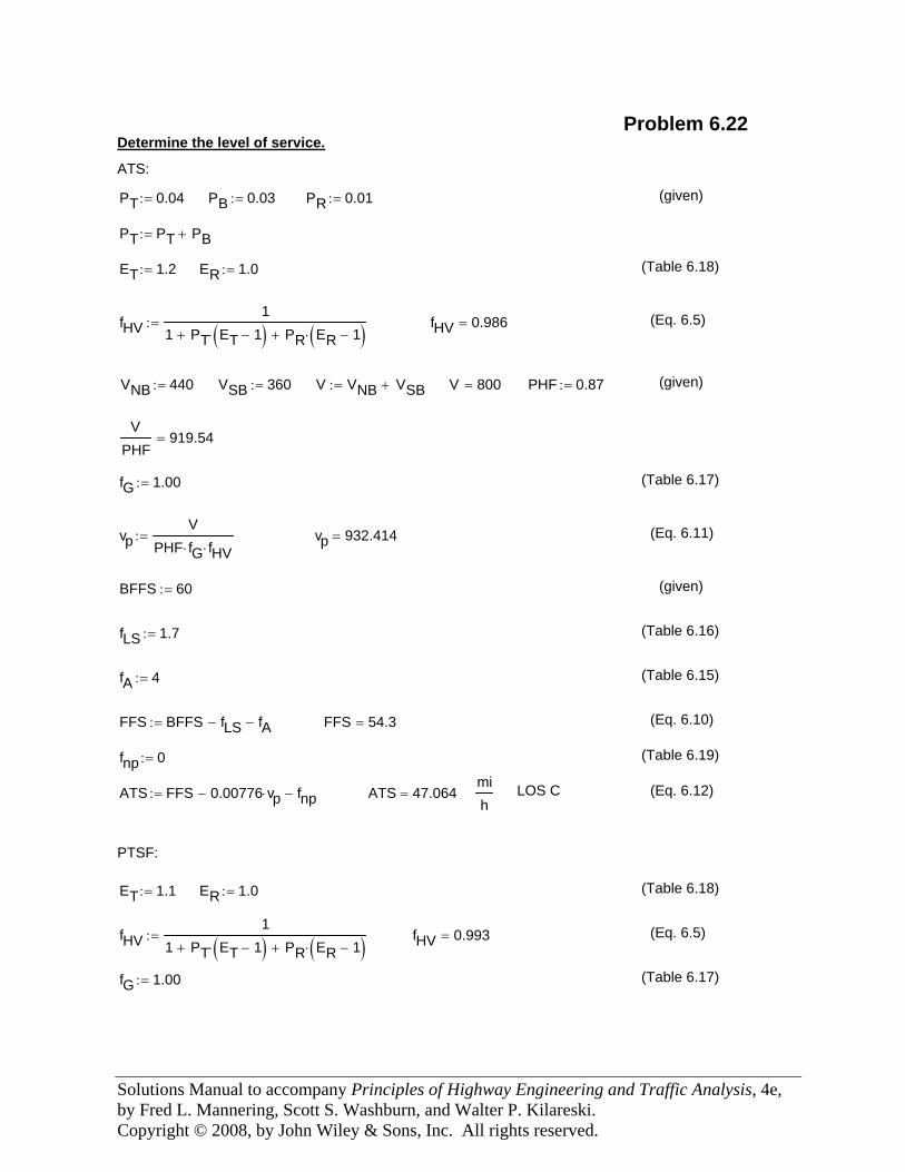
Solutions Manual to accompany Principles of Highway Engineering and Traffic Analysis, 4e, by Fred L. Mannering, Scott S. Washburn, and Walter P. Kilareski. Copyright © 2008, by John Wiley & Sons, Inc. All rights reserved.
BFFS 60:= (given)
fLS 1.7:= (Table 6.16)
fA 4:= (Table 6.15)
FFS BFFS fLS− fA−:= FFS 54.3= (Eq. 6.10)
fnp 0:= (Table 6.19)
ATS FFS 0.00776 vp⋅− fnp−:= ATS 47.064=mih
LOS C (Eq. 6.12)
PTSF:
ET 1.1:= ER 1.0:= (Table 6.18)
fHV1
1 PT ET 1−( )⋅+ PR ER 1−( )⋅+:= fHV 0.993= (Eq. 6.5)
fG 1.00:= (Table 6.17)
Problem 6.22 Determine the level of service.
ATS:
PT 0.04:= PB 0.03:= PR 0.01:= (given)
PT PT PB+:=
ET 1.2:= ER 1.0:= (Table 6.18)
fHV1
1 PT ET 1−( )⋅+ PR ER 1−( )⋅+:= fHV 0.986= (Eq. 6.5)
VNB 440:= VSB 360:= V VNB VSB+:= V 800= PHF 0.87:= (given)
VPHF
919.54=
fG 1.00:= (Table 6.17)
vpV
PHF fG⋅ fHV⋅:= vp 932.414= (Eq. 6.11)
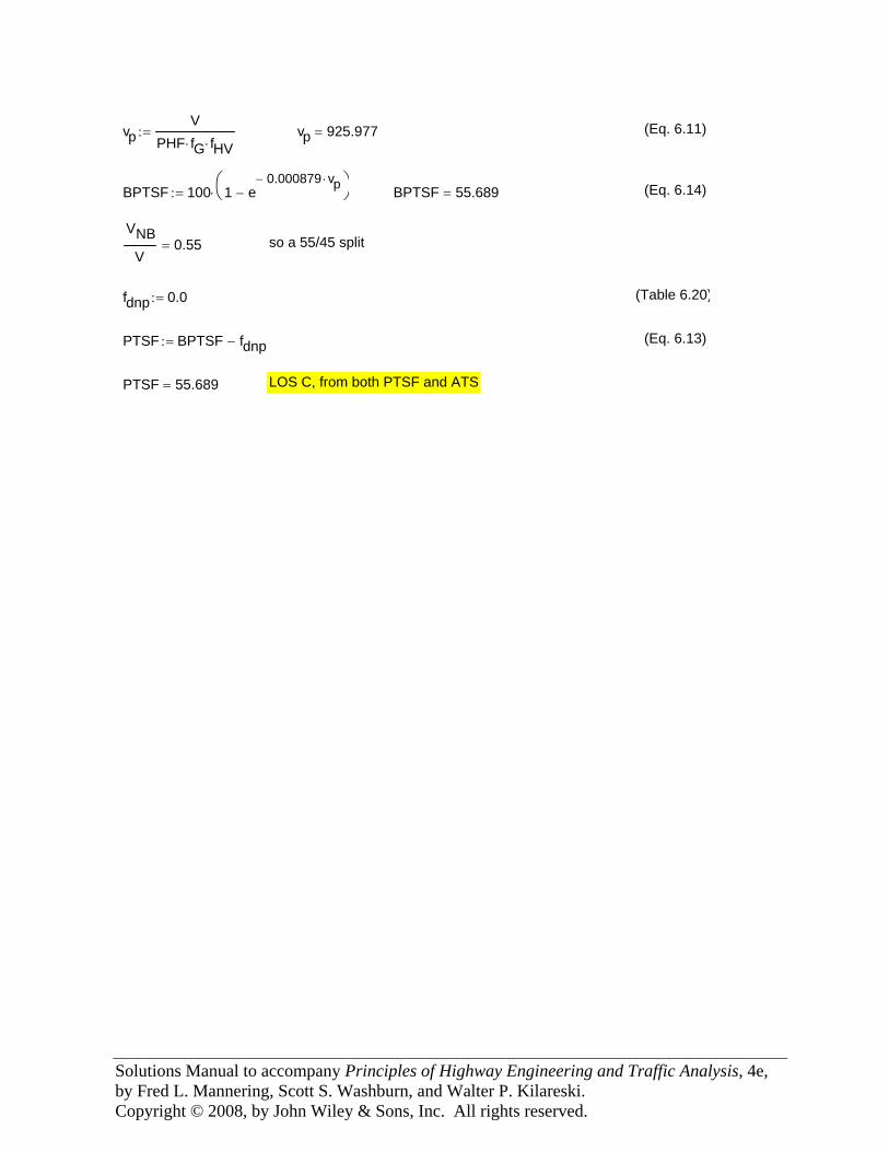
Solutions Manual to accompany Principles of Highway Engineering and Traffic Analysis, 4e, by Fred L. Mannering, Scott S. Washburn, and Walter P. Kilareski. Copyright © 2008, by John Wiley & Sons, Inc. All rights reserved.
vpV
PHF fG⋅ fHV⋅:= vp 925.977= (Eq. 6.11)
BPTSF 100 1 e0.000879− vp⋅
−⎛⎝
⎞⎠⋅:= BPTSF 55.689= (Eq. 6.14)
VNBV
0.55= so a 55/45 split
fdnp 0.0:= (Table 6.20)
PTSF BPTSF fdnp−:= (Eq. 6.13)
PTSF 55.689= LOS C, from both PTSF and ATS
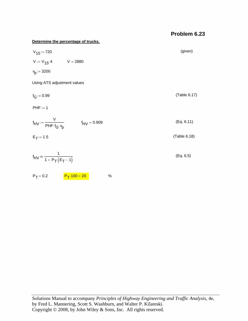
Solutions Manual to accompany Principles of Highway Engineering and Traffic Analysis, 4e, by Fred L. Mannering, Scott S. Washburn, and Walter P. Kilareski. Copyright © 2008, by John Wiley & Sons, Inc. All rights reserved.
%PT 100⋅ 20=PT 0.2=
(Eq. 6.5)fHV1
1 PT ET 1−( )⋅+
(Table 6.18)ET 1.5:=
(Eq. 6.11)fHV 0.909=fHVV
PHF fG⋅ vp⋅:=
PHF 1:=
(Table 6.17)fG 0.99:=
Using ATS adjustment values
vp 3200:=
V 2880=V V15 4⋅:=
(given)V15 720:=
Determine the percentage of trucks.
Problem 6.23
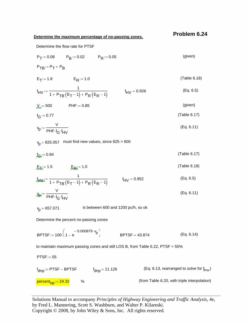
Solutions Manual to accompany Principles of Highway Engineering and Traffic Analysis, 4e, by Fred L. Mannering, Scott S. Washburn, and Walter P. Kilareski. Copyright © 2008, by John Wiley & Sons, Inc. All rights reserved.
Problem 6.24 Determine the maximum percentage of no-passing zones.
Determine the flow rate for PTSF
PT 0.08:= PB 0.02:= PR 0.05:= (given)
PTB PT PB+:=
ET 1.8:= ER 1.0:= (Table 6.18)
fHV1
1 PTB ET 1−( )⋅+ PR ER 1−( )⋅+:= fHV 0.926= (Eq. 6.5)
V 500:= PHF 0.85:= (given)
fG 0.77:= (Table 6.17)
vpV
PHF fG⋅ fHV⋅:= (Eq. 6.11)
vp 825.057= must find new values, since 825 > 600
fG 0.94:= (Table 6.17)
ET 1.5:= ER 1.0:= (Table 6.18)
fHV1
1 PTB ET 1−( )⋅+ PR ER 1−( )⋅+:= fHV 0.952= (Eq. 6.5)
vpV
PHF fG⋅ fHV⋅:= (Eq. 6.11)
vp 657.071= is between 600 and 1200 pc/h, so ok
Determine the percent no-passing zones
BPTSF 100 1 e0.000879− vp⋅
−⎛⎝
⎞⎠⋅:= BPTSF 43.874= (Eq. 6.14)
to maintain maximum passing zones and still LOS B, from Table 6.22, PTSF = 55%
PTSF 55:=
fdnp PTSF BPTSF−:= fdnp 11.126= (Eq. 6.13, rearranged to solve for fd/np )
percentnp 24.32:= % (from Table 6.20, with triple interpolation)
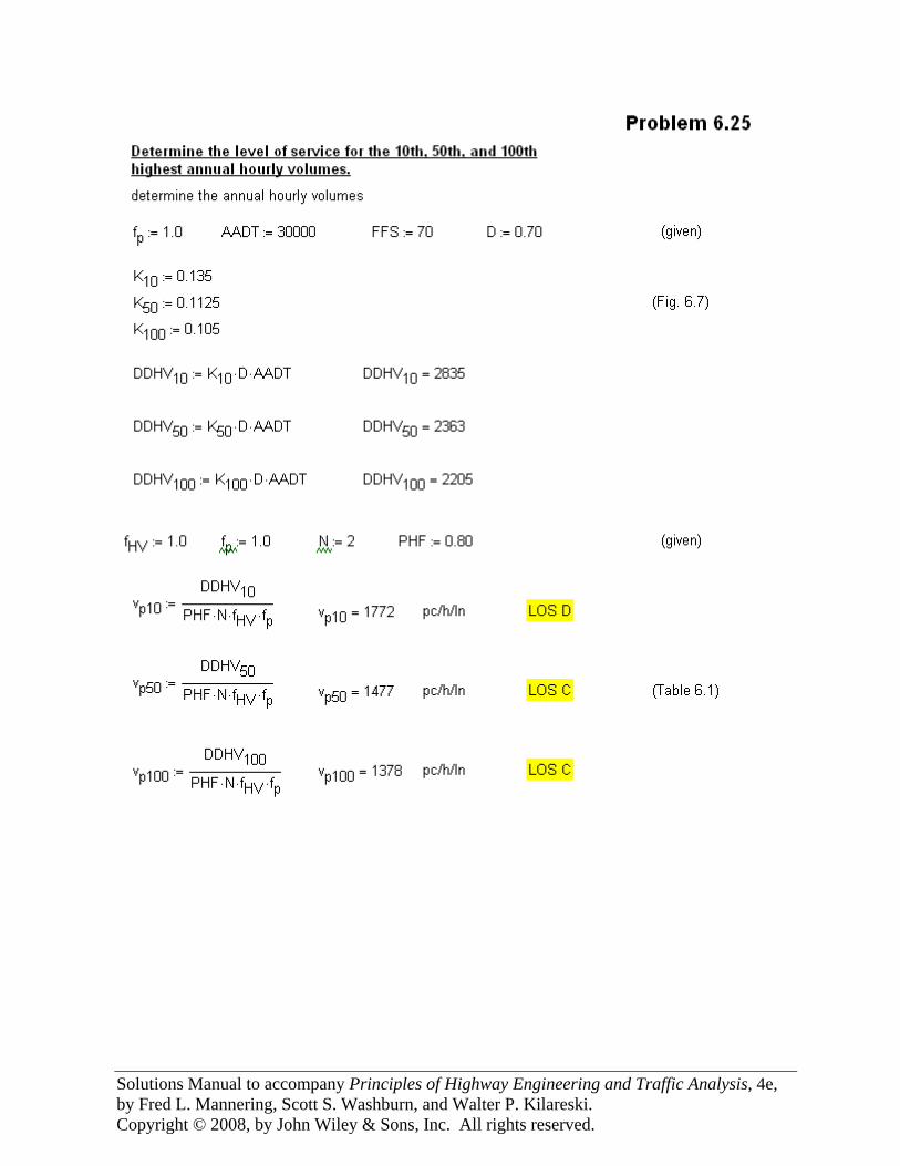
Solutions Manual to accompany Principles of Highway Engineering and Traffic Analysis, 4e, by Fred L. Mannering, Scott S. Washburn, and Walter P. Kilareski. Copyright © 2008, by John Wiley & Sons, Inc. All rights reserved.
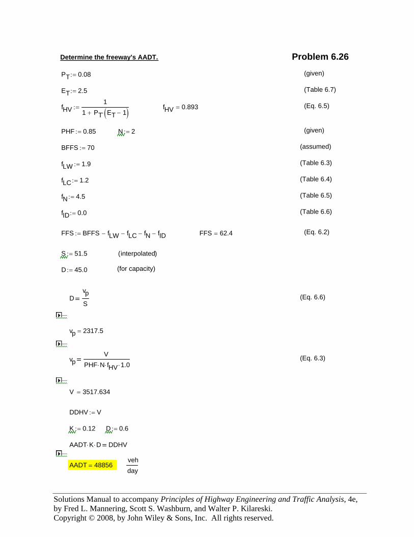
Solutions Manual to accompany Principles of Highway Engineering and Traffic Analysis, 4e, by Fred L. Mannering, Scott S. Washburn, and Walter P. Kilareski. Copyright © 2008, by John Wiley & Sons, Inc. All rights reserved.
Determine the freeway's AADT. Problem 6.26
PT 0.08:= (given)
ET 2.5:= (Table 6.7)
fHV1
1 PT ET 1−( )⋅+:= fHV 0.893= (Eq. 6.5)
PHF 0.85:= N 2:= (given)
BFFS 70:= (assumed)
fLW 1.9:= (Table 6.3)
fLC 1.2:= (Table 6.4)
fN 4.5:= (Table 6.5)
fID 0.0:= (Table 6.6)
FFS BFFS fLW− fLC− fN− fID−:= FFS 62.4= (Eq. 6.2)
S 51.5:= interpolated( )
D 45.0:= (for capacity)
DvpS
(Eq. 6.6)
vp 2317.5=
vpV
PHF N⋅ fHV⋅ 1.0⋅(Eq. 6.3)
V 3517.634=
DDHV V:=
K 0.12:= D 0.6:=
AADT K⋅ D⋅ DDHV
AADT 48856=vehday
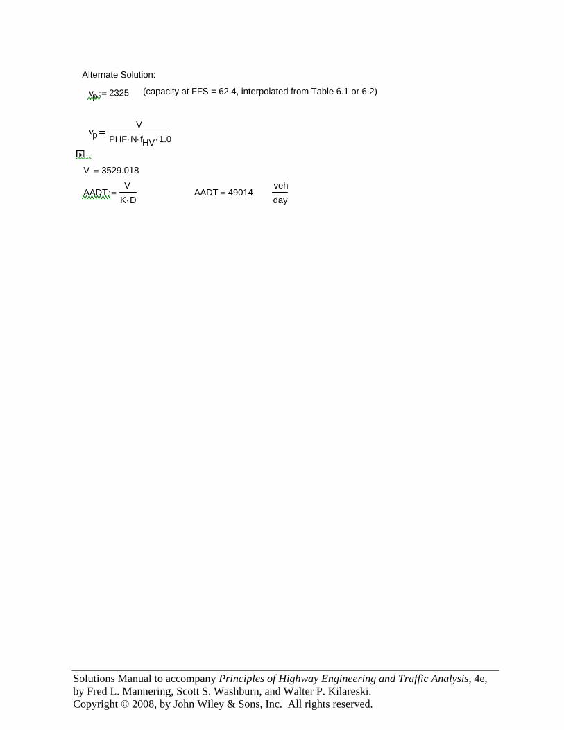
Solutions Manual to accompany Principles of Highway Engineering and Traffic Analysis, 4e, by Fred L. Mannering, Scott S. Washburn, and Walter P. Kilareski. Copyright © 2008, by John Wiley & Sons, Inc. All rights reserved.
Alternate Solution:
vp 2325:= (capacity at FFS = 62.4, interpolated from Table 6.1 or 6.2)
vpV
PHF N⋅ fHV⋅ 1.0⋅
V 3529.018=
AADTV
K D⋅:= AADT 49014=
vehday
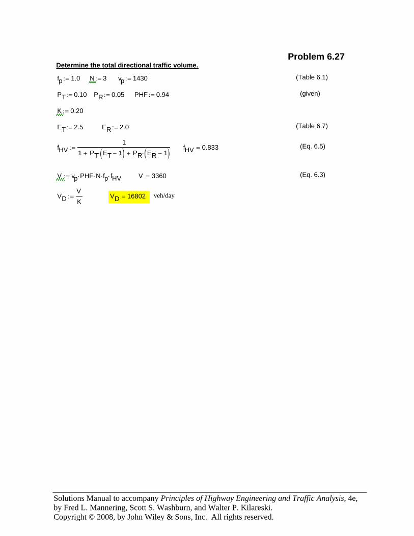
Solutions Manual to accompany Principles of Highway Engineering and Traffic Analysis, 4e, by Fred L. Mannering, Scott S. Washburn, and Walter P. Kilareski. Copyright © 2008, by John Wiley & Sons, Inc. All rights reserved.
Problem 6.27 Determine the total directional traffic volume.
fp 1.0:= N 3:= vp 1430:= (Table 6.1)
PT 0.10:= PR 0.05:= PHF 0.94:= (given)
K 0.20:=
ET 2.5:= ER 2.0:= (Table 6.7)
fHV1
1 PT ET 1−( )⋅+ PR ER 1−( )⋅+:= fHV 0.833= (Eq. 6.5)
V vp PHF⋅ N⋅ fp⋅ fHV⋅:= V 3360= (Eq. 6.3)
VDVK
:= VD 16802= veh/day
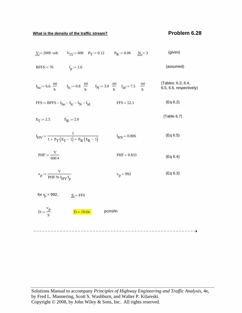
Solutions Manual to accompany Principles of Highway Engineering and Traffic Analysis, 4e, by Fred L. Mannering, Scott S. Washburn, and Walter P. Kilareski. Copyright © 2008, by John Wiley & Sons, Inc. All rights reserved.
What is the density of the traffic stream? Problem 6.28
V 2000:= veh V15 600:= PT 0.12:= PR 0.06:= N 3:= (given)
BFFS 70:= fp 1.0:= (assumed)
(Tables: 6.3, 6.4,6.5, 6.6, respectively)flw 6.6:=
mih
flc 0.8:=mih
fN 3.0:=mih
fid 7.5:=mih
FFS BFFS flw− flc− fN− fid−:= FFS 52.1= (Eq 6.2)
(Table 6.7)ET 2.5:= ER 2.0:=
fHV1
1 PT ET 1−( )⋅+ PR ER 1−( )⋅+:= fHV 0.806= (Eq 6.5)
PHFV
600 4⋅:= PHF 0.833= (Eq 6.4)
vpV
PHF N⋅ fHV⋅ fp⋅:= vp 992= (Eq 6.3)
for vp = 992, S FFS:=
DvpS
:= D 19.04= pc/mi/ln
−−−−−−−−−−−−−−−−−−−−−−−−−−−−−−−−−−−−−−−−−−−−−−−−−−−−−−−
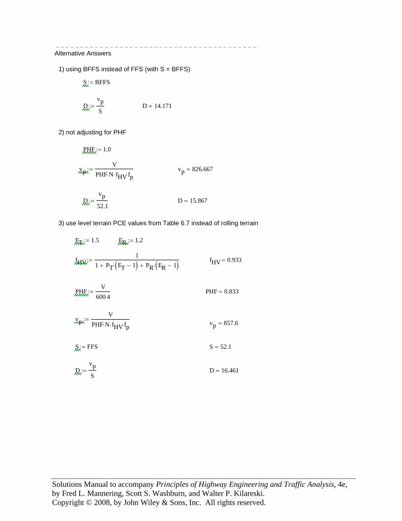
Solutions Manual to accompany Principles of Highway Engineering and Traffic Analysis, 4e, by Fred L. Mannering, Scott S. Washburn, and Walter P. Kilareski. Copyright © 2008, by John Wiley & Sons, Inc. All rights reserved.
−−−−−−−−−−−−−−−−−−−−−−−−−−−−−−−−−−−−−−−−−−Alternative Answers
1) using BFFS instead of FFS (with S = BFFS)
S BFFS:=
DvpS
:= D 14.171=
2) not adjusting for PHF
PHF 1.0:=
vpV
PHF N⋅ fHV⋅ fp⋅:= vp 826.667=
Dvp52.1
:= D 15.867=
3) use level terrain PCE values from Table 6.7 instead of rolling terrain
ET 1.5:= ER 1.2:=
fHV1
1 PT ET 1−( )⋅+ PR ER 1−( )⋅+:= fHV 0.933=
PHFV
600 4⋅:= PHF 0.833=
vpV
PHF N⋅ fHV⋅ fp⋅:= vp 857.6=
S FFS:= S 52.1=
DvpS
:= D 16.461=
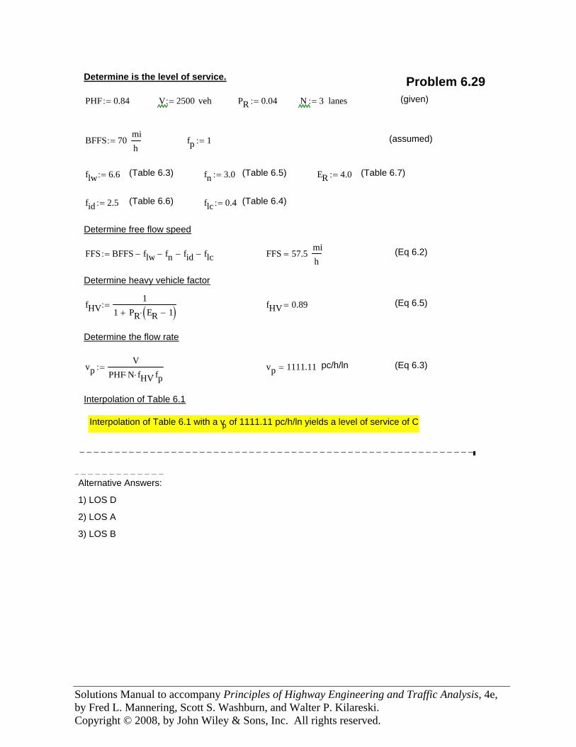
Solutions Manual to accompany Principles of Highway Engineering and Traffic Analysis, 4e, by Fred L. Mannering, Scott S. Washburn, and Walter P. Kilareski. Copyright © 2008, by John Wiley & Sons, Inc. All rights reserved.
Determine is the level of service. Problem 6.29PHF 0.84:= V 2500:= veh PR 0.04:= N 3:= lanes (given)
BFFS 70:=mih
fp 1:= (assumed)
flw 6.6:= (Table 6.3) fn 3.0:= (Table 6.5) ER 4.0:= (Table 6.7)
fid 2.5:= (Table 6.6) flc 0.4:= (Table 6.4)
Determine free flow speed
FFS BFFS flw− fn− fid− flc−:= FFS 57.5=mih
(Eq 6.2)
Determine heavy vehicle factor
fHV1
1 PR ER 1−( )⋅+:= fHV 0.89= (Eq 6.5)
Determine the flow rate
vpV
PHF N⋅ fHV⋅ fp⋅:= vp 1111.11= pc/h/ln (Eq 6.3)
Interpolation of Table 6.1
Interpolation of Table 6.1 with a vp of 1111.11 pc/h/ln yields a level of service of C
−−−−−−−−−−−−−−−−−−−−−−−−−−−−−−−−−−−−−−−−−−−−−−−−−−−−−−−− −−−−−−−−−−−−−Alternative Answers:
1) LOS D
2) LOS A
3) LOS B
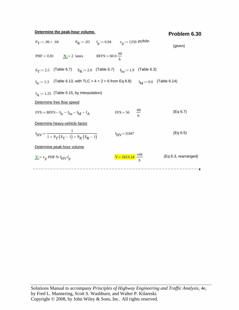
Solutions Manual to accompany Principles of Highway Engineering and Traffic Analysis, 4e, by Fred L. Mannering, Scott S. Washburn, and Walter P. Kilareski. Copyright © 2008, by John Wiley & Sons, Inc. All rights reserved.
Determine the peak-hour volume. Problem 6.30PT .06 .04+:= PR .03:= fp 0.94:= vp 1250:= pc/h/ln
(given)
PHF 0.81:= N 2:= lanes BFFS 60.0:=mih
ET 2.5:= (Table 6.7) ER 2.0:= (Table 6.7) flw 1.9:= (Table 6.3)
flc 1.3:= (Table 6.13, with TLC = 4 + 2 = 6 from Eq 6.8) fM 0.0:= (Table 6.14)
fA 1.25:= (Table 6.15, by interpolation)
Determine free flow speed
FFS BFFS flc− flw− fM− fA−:= FFS 56=mih
(Eq 6.7)
Determine heavy-vehicle factor
fHV1
1 PT ET 1−( )⋅+ PR ER 1−( )⋅+:= fHV 0.847= (Eq 6.5)
Determine peak-hour volume
V vp PHF⋅ N⋅ fHV⋅ fp⋅:= V 1613.14=vehh
(Eq 6.3, rearranged)
−−−−−−−−−−−−−−−−−−−−−−−−−−−−−−−−−−−−−−−−−−−−−−−−−−−−−−−−−
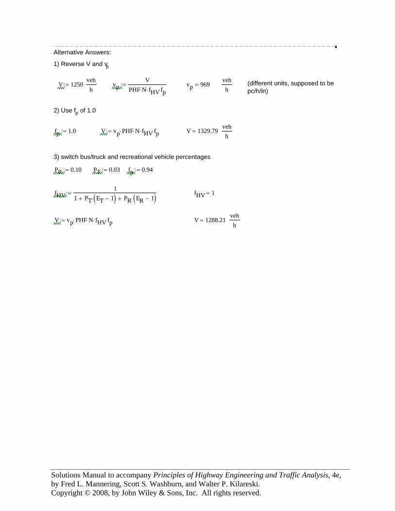
Solutions Manual to accompany Principles of Highway Engineering and Traffic Analysis, 4e, by Fred L. Mannering, Scott S. Washburn, and Walter P. Kilareski. Copyright © 2008, by John Wiley & Sons, Inc. All rights reserved.
−−−−−−−−−−−−−−−−−−−−−−−−−−−−−−−−−−−−−−−−−−−−−−−−−−−−−−−−−−−Alternative Answers:
1) Reverse V and vp
V 1250:=vehh
vpV
PHF N⋅ fHV⋅ fp⋅:= vp 969=
vehh
(different units, supposed to bepc/h/ln)
2) Use fp of 1.0
fp 1.0:= V vp PHF⋅ N⋅ fHV⋅ fp⋅:= V 1329.79=vehh
3) switch bus/truck and recreational vehicle percentages
PR 0.10:= PT 0.03:= fp 0.94:=
fHV1
1 PT ET 1−( )⋅+ PR ER 1−( )⋅+:= fHV 1=
V vp PHF⋅ N⋅ fHV⋅ fp⋅:= V 1288.21=vehh
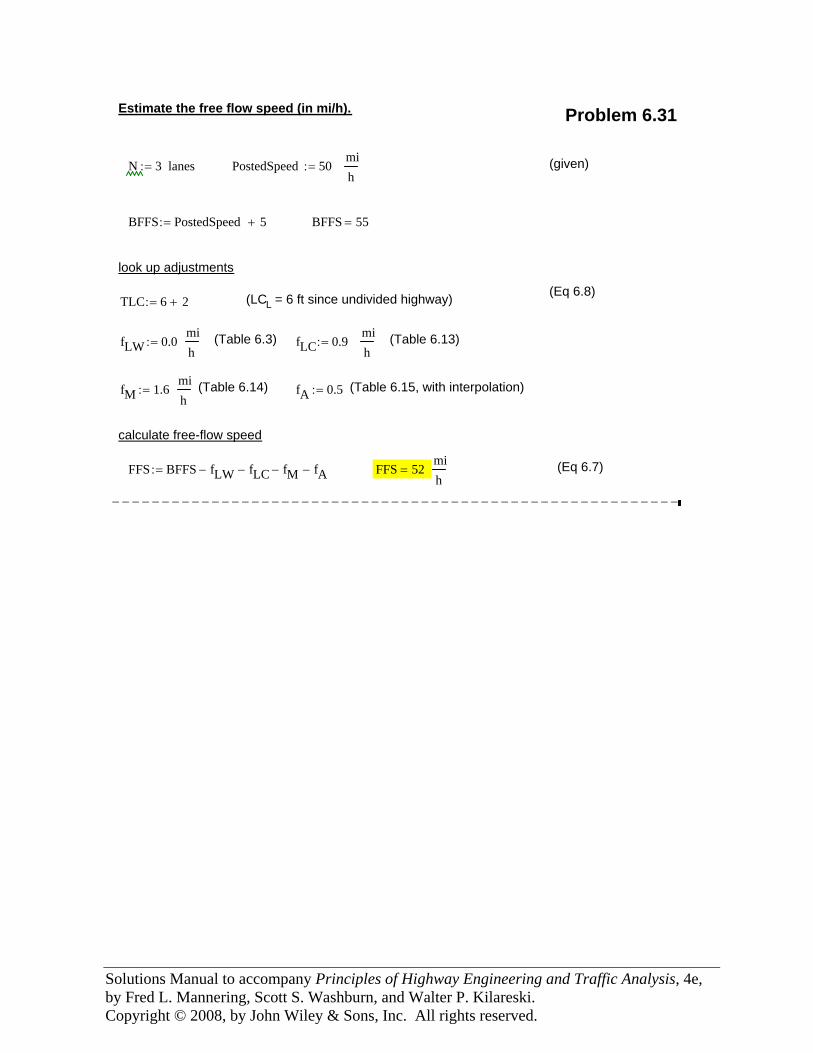
Solutions Manual to accompany Principles of Highway Engineering and Traffic Analysis, 4e, by Fred L. Mannering, Scott S. Washburn, and Walter P. Kilareski. Copyright © 2008, by John Wiley & Sons, Inc. All rights reserved.
Estimate the free flow speed (in mi/h). Problem 6.31
N 3:= lanes PostedSpeed 50:=mih
(given)
BFFS PostedSpeed 5+:= BFFS 55=
look up adjustments
(Eq 6.8)TLC 6 2+:= (LCL = 6 ft since undivided highway)
fLW 0.0:=mih
(Table 6.3) fLC 0.9:=mih
(Table 6.13)
fM 1.6:=mih
(Table 6.14) fA 0.5:= (Table 6.15, with interpolation)
calculate free-flow speed
FFS BFFS fLW− fLC− fM− fA−:= FFS 52=mih
(Eq 6.7)
−−−−−−−−−−−−−−−−−−−−−−−−−−−−−−−−−−−−−−−−−−−−−−−−−−−−−−−−−
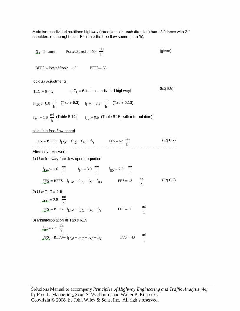
Solutions Manual to accompany Principles of Highway Engineering and Traffic Analysis, 4e, by Fred L. Mannering, Scott S. Washburn, and Walter P. Kilareski. Copyright © 2008, by John Wiley & Sons, Inc. All rights reserved.
A six-lane undivided multilane highway (three lanes in each direction) has 12-ft lanes with 2-ftshoulders on the right side. Estimate the free flow speed (in mi/h).
N 3:= lanes PostedSpeed 50:=mih
(given)
BFFS PostedSpeed 5+:= BFFS 55=
look up adjustments
(Eq 6.8)TLC 6 2+:= (LCL = 6 ft since undivided highway)
fLW 0.0:=mih
(Table 6.3) fLC 0.9:=mih
(Table 6.13)
fM 1.6:=mih
(Table 6.14) fA 0.5:= (Table 6.15, with interpolation)
calculate free-flow speed
FFS BFFS fLW− fLC− fM− fA−:= FFS 52=mih
(Eq 6.7)
−−−−−−−−−−−−−−−−−−−−−−−−−−−−−−−−−−−−−−−−−−−−−−−−−−Alternative Answers
1) Use freeway free-flow speed equation
fLC 1.6:=mih
fN 3.0:=mih
fID 7.5:=mih
FFS BFFS fLW− fLC− fN− fID−:= FFS 43=mih
(Eq 6.2)
2) Use TLC = 2-ft
fLC 2.8:=mih
FFS BFFS fLW− fLC− fM− fA−:= FFS 50=mih
3) Misinterpolation of Table 6.15
fA 2.5:=mih
FFS BFFS fLW− fLC− fM− fA−:= FFS 48=mih
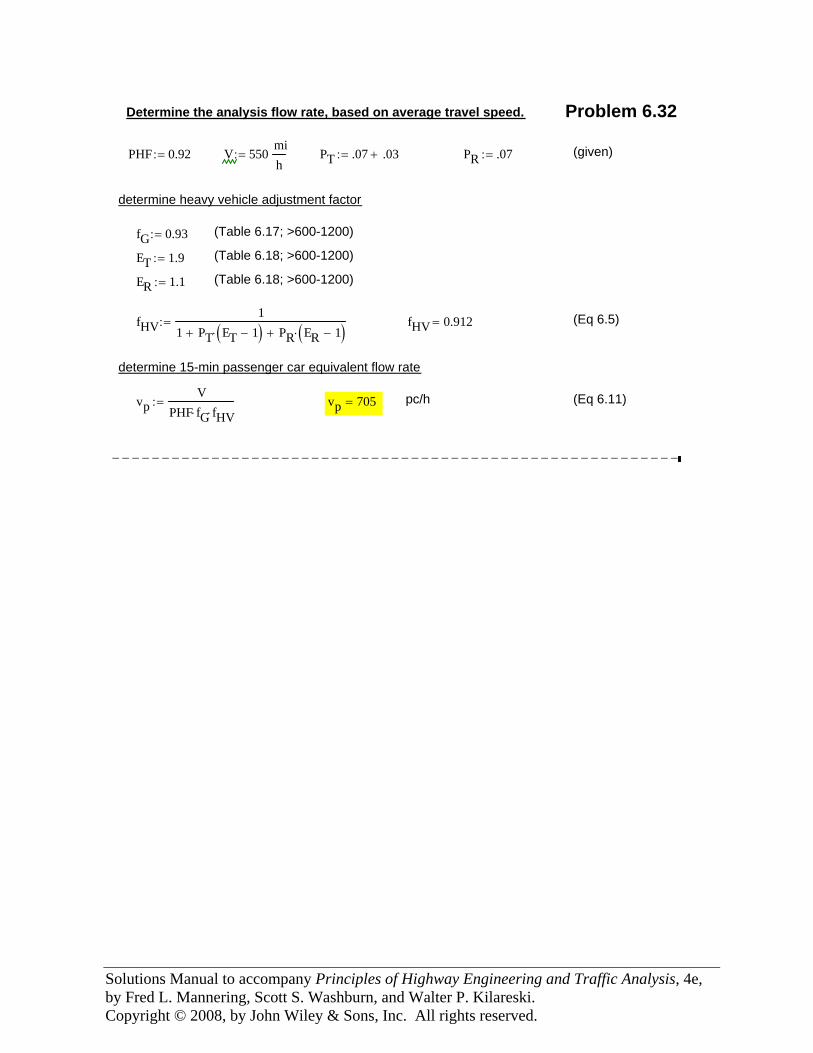
Solutions Manual to accompany Principles of Highway Engineering and Traffic Analysis, 4e, by Fred L. Mannering, Scott S. Washburn, and Walter P. Kilareski. Copyright © 2008, by John Wiley & Sons, Inc. All rights reserved.
Determine the analysis flow rate, based on average travel speed. Problem 6.32
PHF 0.92:= V 550:=mih
PT .07 .03+:= PR .07:= (given)
determine heavy vehicle adjustment factor
fG 0.93:= (Table 6.17; >600-1200)
ET 1.9:= (Table 6.18; >600-1200)
ER 1.1:= (Table 6.18; >600-1200)
fHV1
1 PT ET 1−( )⋅+ PR ER 1−( )⋅+:= fHV 0.912= (Eq 6.5)
determine 15-min passenger car equivalent flow rate
vpV
PHF fG⋅ fHV⋅:= vp 705= pc/h (Eq 6.11)
−−−−−−−−−−−−−−−−−−−−−−−−−−−−−−−−−−−−−−−−−−−−−−−−−−−−−−−−−
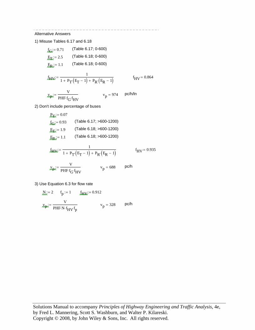
Solutions Manual to accompany Principles of Highway Engineering and Traffic Analysis, 4e, by Fred L. Mannering, Scott S. Washburn, and Walter P. Kilareski. Copyright © 2008, by John Wiley & Sons, Inc. All rights reserved.
−−−−−−−−−−−−−−−−−−−−−−−−−−−−−−−−−−−−−−−−−Alternative Answers
1) Misuse Tables 6.17 and 6.18
fG 0.71:= (Table 6.17; 0-600)
ET 2.5:= (Table 6.18; 0-600)
ER 1.1:= (Table 6.18; 0-600)
fHV1
1 PT ET 1−( )⋅+ PR ER 1−( )⋅+:= fHV 0.864=
vpV
PHF fG⋅ fHV⋅:= vp 974= pc/h/ln
2) Don't include percentage of buses
PT 0.07:=
fG 0.93:= (Table 6.17; >600-1200)
ET 1.9:= (Table 6.18; >600-1200)
ER 1.1:= (Table 6.18; >600-1200)
fHV1
1 PT ET 1−( )⋅+ PR ER 1−( )⋅+:= fHV 0.935=
vpV
PHF fG⋅ fHV⋅:= vp 688= pc/h
3) Use Equation 6.3 for flow rate
N 2:= fp 1:= fHV 0.912:=
vpV
PHF N⋅ fHV⋅ fp⋅:= vp 328= pc/h
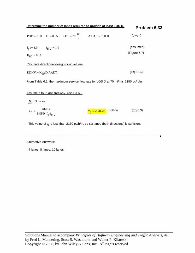
Solutions Manual to accompany Principles of Highway Engineering and Traffic Analysis, 4e, by Fred L. Mannering, Scott S. Washburn, and Walter P. Kilareski. Copyright © 2008, by John Wiley & Sons, Inc. All rights reserved.
Determine the number of lanes required to provide at least LOS D. Problem 6.33
PHF 0.88:= D 0.65:= FFS 70:=mih
AADT 75000:= (given)
fp 1.0:= fHV 1.0:= (assumed)
(Figure 6.7)K60 0.11:=
Calculate directional design-hour volume
DDHV K60 D⋅ AADT⋅:= (Eq 6.16)
From Table 6.1, the maximum service flow rate for LOS D at 70 mi/h is 2150 pc/h/ln.
Assume a four-lane freeway. Use Eq 6.3
N 3:= lanes
vpDDHV
PHF N⋅ fp⋅ fHV⋅:= vp 2031.25= pc/h/ln (Eq 6.3)
This value of vp is less than 2150 pc/h/ln, so six lanes (both directions) is sufficient.
−−−−−−−−−−−−−−−−−−−−−−−−−−−−−−−−−−−−−−−−−−−−−−−−−−−−−−−−−−−−−−−−−−−−−−−−−
Alternative Answers:
4 lanes, 8 lanes, 10 lanes
Solutions Manual to accompany
Principles of Highway Engineering and Traffic Analysis, 4e
By Fred L. Mannering, Scott S. Washburn, and Walter P. Kilareski
Chapter 7 Traffic Control and Analysis at
Signalized Intersections
U.S. Customary Units
Copyright © 2008, by John Wiley & Sons, Inc. All rights reserved.

Solutions Manual to accompany Principles of Highway Engineering and Traffic Analysis, 4e, by Fred L. Mannering, Scott S. Washburn, and Walter P. Kilareski. Copyright © 2008, by John Wiley & Sons, Inc. All rights reserved.
Preface The solutions to the fourth edition of Principles of Highway Engineering and Traffic Analysis were prepared with the Mathcad1 software program. You will notice several notation conventions that you may not be familiar with if you are not a Mathcad user. Most of these notation conventions are self-explanatory or easily understood. The most common Mathcad specific notations in these solutions relate to the equals sign. You will notice the equals sign being used in three different contexts, and Mathcad uses three different notations to distinguish between each of these contexts. The differences between these equals sign notations are explained as follows.
• The ‘:=’ (colon-equals) is an assignment operator, that is, the value of the variable or expression on the left side of ‘:=’is set equal to the value of the expression on the right side. For example, in the statement, L := 1234, the variable ‘L’ is assigned (i.e., set equal to) the value of 1234. Another example is x := y + z. In this case, x is assigned the value of y + z.
• The ‘==’ (bold equals) is used when the Mathcad function solver was used to find the value of a variable in the equation. For example, in the equation
, the == is used to tell Mathcad that the value of the expression on the left side needs to equal the value of the expression on the right side. Thus, the Mathcad solver can be employed to find a value for the variable ‘t’ that satisfies this relationship. This particular example is from a problem where the function for arrivals at some time ‘t’ is set equal to the function for departures at some time ‘t’ to find the time to queue clearance.
• The ‘=’ (standard equals) is used for a simple numeric evaluation. For example, referring to the x := y + z assignment used previously, if the value of y was 10 [either by assignment (with :=), or the result of an equation solution (through the use of ==) and the value of z was 15, then the expression ‘x =’ would yield 25. Another example would be as follows: s := 1800/3600, with s = 0.5. That is, ‘s’ was assigned the value of 1800 divided by 3600 (using :=), which equals 0.5 (as given by using =).
Another symbol you will see frequently is ‘→’. In these solutions, it is used to perform an evaluation of an assignment expression in a single statement. For example, in the following
statement, , Q(t) is assigned the value of Arrivals(t) – Departures(t), and this evaluates to 2.2t – 0.10t2. Finally, to assist in quickly identifying the final answer, or answers, for what is being asked in the problem statement, yellow highlighting has been used (which will print as light gray). 1 www.mathcad.com
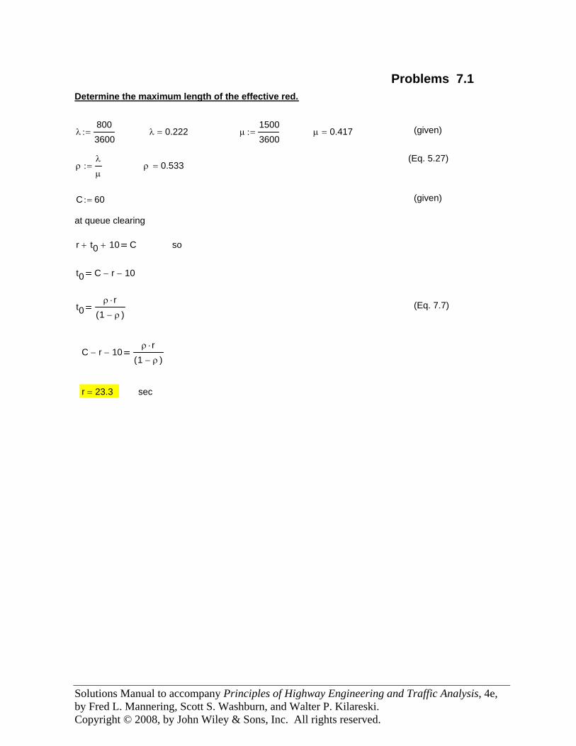
Solutions Manual to accompany Principles of Highway Engineering and Traffic Analysis, 4e, by Fred L. Mannering, Scott S. Washburn, and Walter P. Kilareski. Copyright © 2008, by John Wiley & Sons, Inc. All rights reserved.
secr 23.3=
C r− 10−ρ r⋅
1 ρ−( )
(Eq. 7.7)t0ρ r⋅
1 ρ−( )
t0 C r− 10−
sor t0+ 10+ C
at queue clearing
(given)C 60:=
ρ 0.533=ρλ
μ:=
(Eq. 5.27)
(given)μ 0.417=μ15003600
:=λ 0.222=λ8003600
:=
Determine the maximum length of the effective red.
Problems 7.1
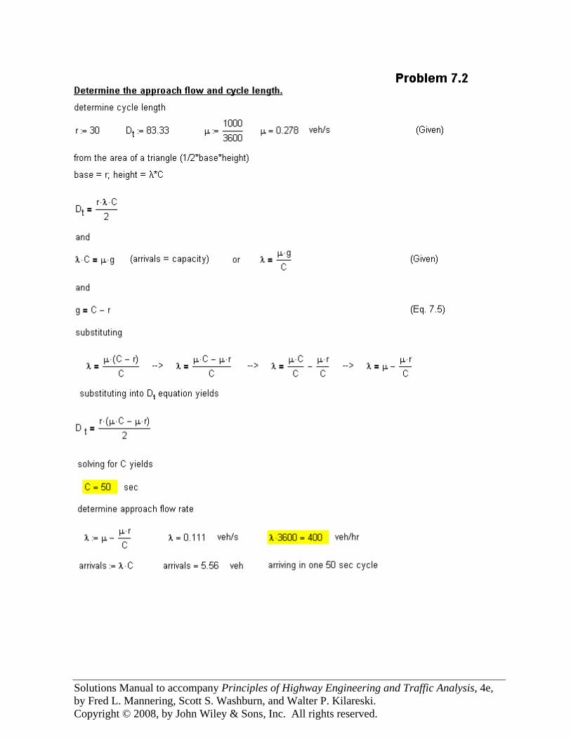
Solutions Manual to accompany Principles of Highway Engineering and Traffic Analysis, 4e, by Fred L. Mannering, Scott S. Washburn, and Walter P. Kilareski. Copyright © 2008, by John Wiley & Sons, Inc. All rights reserved.
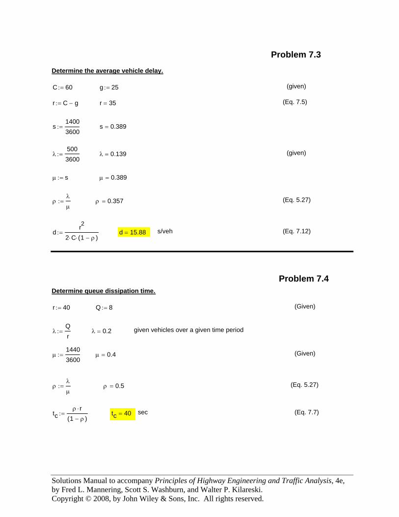
Solutions Manual to accompany Principles of Highway Engineering and Traffic Analysis, 4e, by Fred L. Mannering, Scott S. Washburn, and Walter P. Kilareski. Copyright © 2008, by John Wiley & Sons, Inc. All rights reserved.
(Eq. 7.12)s/vehd 15.88=dr2
2 C⋅ 1 ρ−( )⋅:=
(Eq. 5.27)ρ 0.357=ρλ
μ:=
μ 0.389=μ s:=
(given)λ 0.139=λ5003600
:=
s 0.389=s14003600
:=
(Eq. 7.5)r 35=r C g−:=
(given)g 25:=C 60:=
Determine the average vehicle delay.
Problem 7.3
(Eq. 7.7)sectc 40=tcρ r⋅
1 ρ−( ):=
(Eq. 5.27)ρ 0.5=ρλ
μ:=
(Given)μ 0.4=μ14403600
:=
given vehicles over a given time periodλ 0.2=λQr
:=
(Given)Q 8:=r 40:=
Determine queue dissipation time.
Problem 7.4
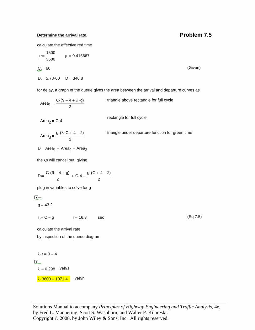
Solutions Manual to accompany Principles of Highway Engineering and Traffic Analysis, 4e, by Fred L. Mannering, Scott S. Washburn, and Walter P. Kilareski. Copyright © 2008, by John Wiley & Sons, Inc. All rights reserved.
Determine the arrival rate. Problem 7.5calculate the effective red time
μ15003600
:= μ 0.416667=
C 60:= (Given)
D 5.78 60⋅:= D 346.8=
for delay, a graph of the queue gives the area between the arrival and departure curves as
triangle above rectangle for full cycleArea1
C 9 4− λ g⋅+( )⋅
2
rectangle for full cycleArea2 C 4⋅
triangle under departure function for green timeArea3
g λ C⋅ 4+ 2−( )⋅
2
D Area1 Area2+ Area3+
the λs will cancel out, giving
DC 9 4− g+( )⋅
2C 4⋅+
g C 4+ 2−( )⋅
2−
plug in variables to solve for g
g 43.2=
r C g−:= r 16.8= sec (Eq 7.5)
calculate the arrival rate
by inspection of the queue diagram
λ r⋅ 9 4−
λ 0.298= veh/s
λ 3600⋅ 1071.4= veh/h
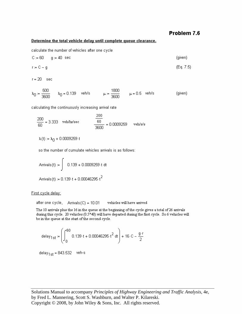
Solutions Manual to accompany Principles of Highway Engineering and Traffic Analysis, 4e, by Fred L. Mannering, Scott S. Washburn, and Walter P. Kilareski. Copyright © 2008, by John Wiley & Sons, Inc. All rights reserved.
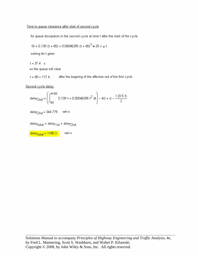
Solutions Manual to accompany Principles of Highway Engineering and Traffic Analysis, 4e, by Fred L. Mannering, Scott S. Washburn, and Walter P. Kilareski. Copyright © 2008, by John Wiley & Sons, Inc. All rights reserved.
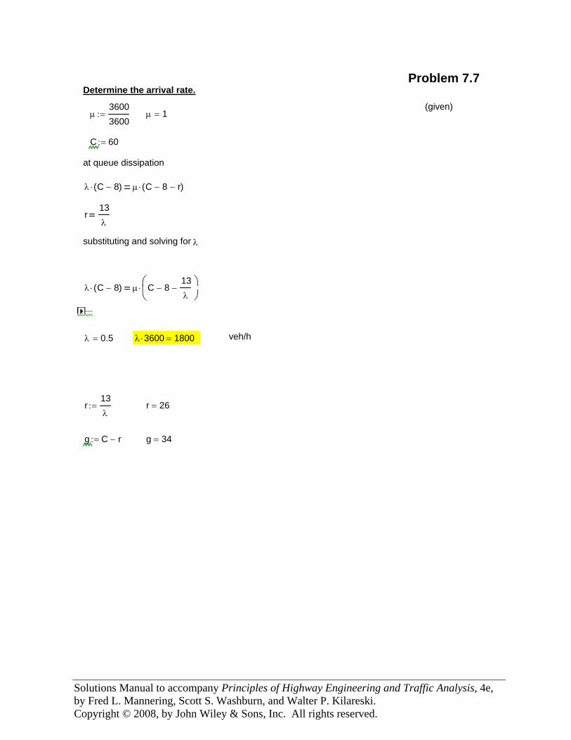
Solutions Manual to accompany Principles of Highway Engineering and Traffic Analysis, 4e, by Fred L. Mannering, Scott S. Washburn, and Walter P. Kilareski. Copyright © 2008, by John Wiley & Sons, Inc. All rights reserved.
Problem 7.7Determine the arrival rate.
(given)μ
36003600
:= μ 1=
C 60:=
at queue dissipation
λ C 8−( )⋅ μ C 8− r−( )⋅
r13λ
substituting and solving for λ
λ C 8−( )⋅ μ C 8−13λ
−⎛⎜⎝
⎞⎟⎠
⋅
λ 0.5= λ 3600⋅ 1800= veh/h
r13λ
:= r 26=
g C r−:= g 34=
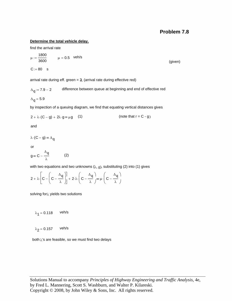
Solutions Manual to accompany Principles of Highway Engineering and Traffic Analysis, 4e, by Fred L. Mannering, Scott S. Washburn, and Walter P. Kilareski. Copyright © 2008, by John Wiley & Sons, Inc. All rights reserved.
both λ's are feasible, so we must find two delays
veh/sλ2 0.157=
veh/sλ1 0.118=
solving for λ yields two solutions
2 λ C CΔqλ
−⎛⎜⎝
⎞⎟⎠
−⎡⎢⎣
⎤⎥⎦
⋅+ 2 λ⋅ CΔqλ
−⎛⎜⎝
⎞⎟⎠
⋅+ μ CΔqλ
−⎛⎜⎝
⎞⎟⎠
⋅
with two equations and two unknowns (λ, g), substituting (2) into (1) gives
(2) g CΔqλ
−
or
λ C g−( )⋅ Δq
and
(note that r = C - g)(1) 2 λ C g−( )⋅+ 2λ g⋅+ μg
by inspection of a queuing diagram, we find that equating vertical distances gives
Δq 5.9=
difference between queue at beginning and end of effective redΔq 7.9 2−:=
arrival rate during eff. green = 2λ (arrival rate during effective red)
sC 80:=
(given)veh/sμ 0.5=μ
18003600
:=
find the arrival rate
Determine the total vehicle delay.
Problem 7.8
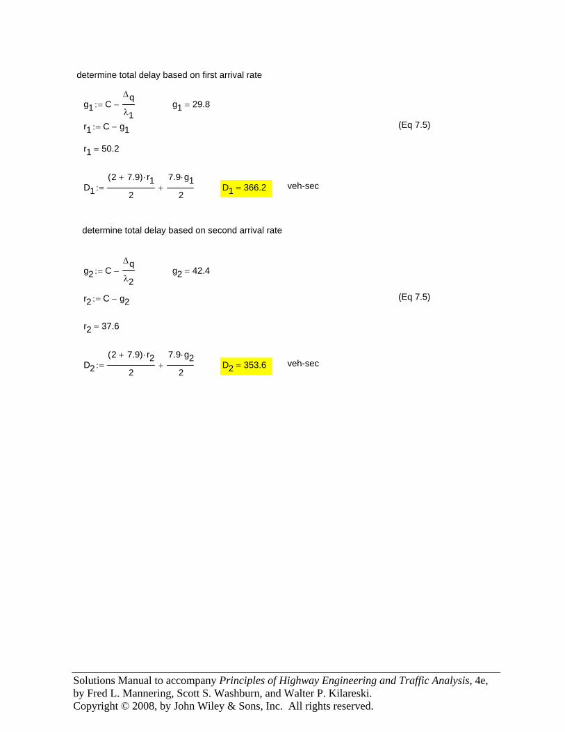
Solutions Manual to accompany Principles of Highway Engineering and Traffic Analysis, 4e, by Fred L. Mannering, Scott S. Washburn, and Walter P. Kilareski. Copyright © 2008, by John Wiley & Sons, Inc. All rights reserved.
veh-secD2 353.6=D22 7.9+( ) r2⋅
2
7.9 g2⋅
2+:=
r2 37.6=
(Eq 7.5)r2 C g2−:=
g2 42.4=g2 CΔqλ2
−:=
determine total delay based on second arrival rate
veh-secD1 366.2=D12 7.9+( ) r1⋅
2
7.9 g1⋅
2+:=
r1 50.2=
(Eq 7.5)r1 C g1−:=
g1 29.8=g1 CΔqλ1
−:=
determine total delay based on first arrival rate
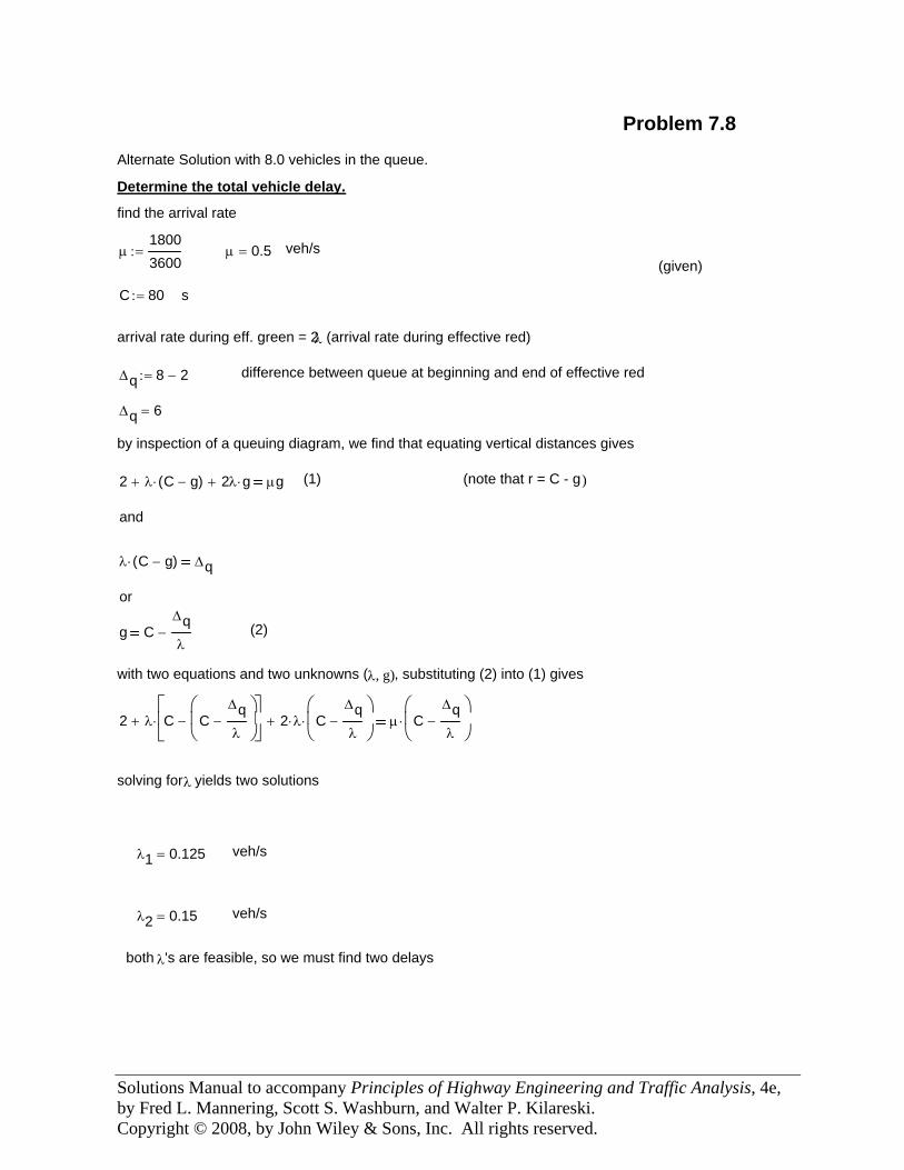
Solutions Manual to accompany Principles of Highway Engineering and Traffic Analysis, 4e, by Fred L. Mannering, Scott S. Washburn, and Walter P. Kilareski. Copyright © 2008, by John Wiley & Sons, Inc. All rights reserved.
both λ's are feasible, so we must find two delays
veh/sλ2 0.15=
veh/sλ1 0.125=
solving for λ yields two solutions
2 λ C CΔqλ
−⎛⎜⎝
⎞⎟⎠
−⎡⎢⎣
⎤⎥⎦
⋅+ 2 λ⋅ CΔqλ
−⎛⎜⎝
⎞⎟⎠
⋅+ μ CΔqλ
−⎛⎜⎝
⎞⎟⎠
⋅
with two equations and two unknowns (λ, g), substituting (2) into (1) gives
(2) g CΔqλ
−
or
λ C g−( )⋅ Δq
and
(note that r = C - g)
Problem 7.8Alternate Solution with 8.0 vehicles in the queue.
Determine the total vehicle delay.
find the arrival rate
μ18003600
:= μ 0.5= veh/s(given)
C 80:= s
arrival rate during eff. green = 2λ (arrival rate during effective red)
Δq 8 2−:= difference between queue at beginning and end of effective red
Δq 6=
by inspection of a queuing diagram, we find that equating vertical distances gives
2 λ C g−( )⋅+ 2λ g⋅+ μg (1)
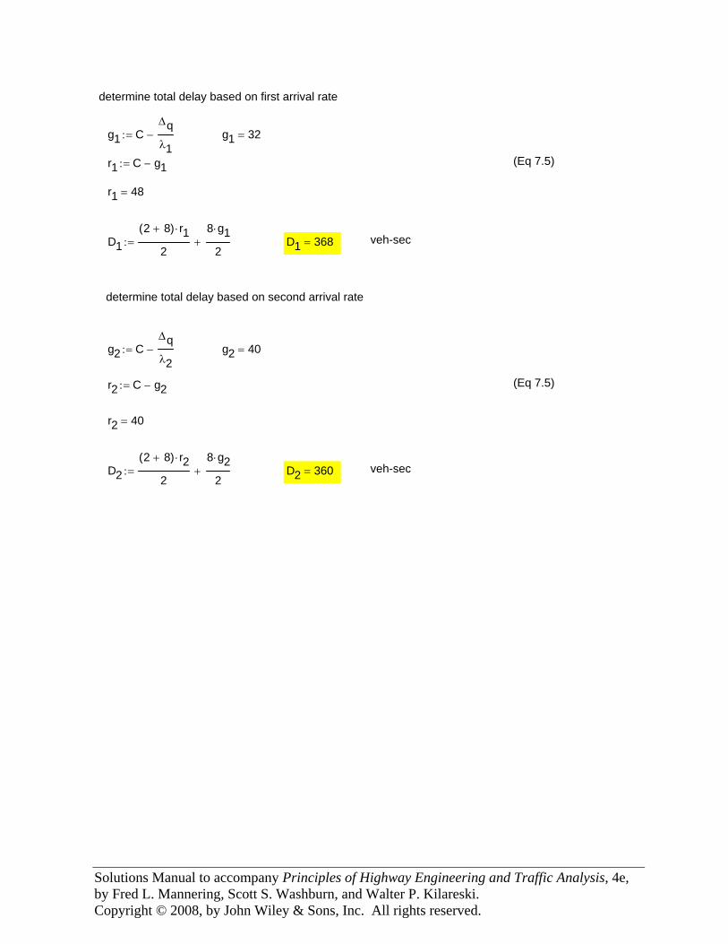
Solutions Manual to accompany Principles of Highway Engineering and Traffic Analysis, 4e, by Fred L. Mannering, Scott S. Washburn, and Walter P. Kilareski. Copyright © 2008, by John Wiley & Sons, Inc. All rights reserved.
veh-secD2 360=D22 8+( ) r2⋅
2
8 g2⋅
2+:=
r2 40=
(Eq 7.5)r2 C g2−:=
g2 40=g2 CΔqλ2
−:=
determine total delay based on second arrival rate
veh-secD1 368=D12 8+( ) r1⋅
2
8 g1⋅
2+:=
r1 48=
(Eq 7.5)r1 C g1−:=
g1 32=g1 CΔqλ1
−:=
determine total delay based on first arrival rate
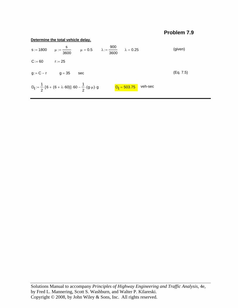
Solutions Manual to accompany Principles of Highway Engineering and Traffic Analysis, 4e, by Fred L. Mannering, Scott S. Washburn, and Walter P. Kilareski. Copyright © 2008, by John Wiley & Sons, Inc. All rights reserved.
veh-secDt 503.75=Dt12
6 6 λ 60⋅+( )+[ ]⋅ 60⋅12
g μ⋅( )⋅ g⋅−:=
(Eq. 7.5)secg 35=g C r−:=
r 25:=C 60:=
(given)λ 0.25=λ9003600
:=μ 0.5=μs
3600:=s 1800:=
Determine the total vehicle delay.
Problem 7.9
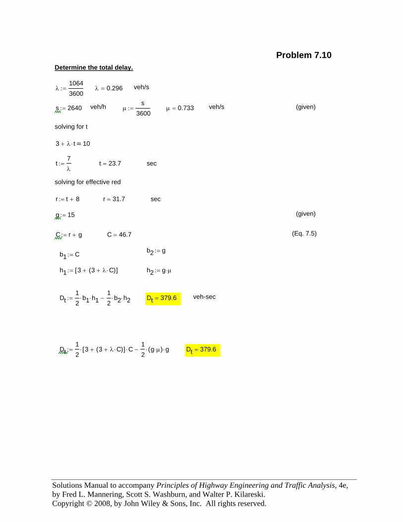
Solutions Manual to accompany Principles of Highway Engineering and Traffic Analysis, 4e, by Fred L. Mannering, Scott S. Washburn, and Walter P. Kilareski. Copyright © 2008, by John Wiley & Sons, Inc. All rights reserved.
Problem 7.10Determine the total delay.
λ10643600
:= λ 0.296= veh/s
s 2640:= veh/h μs
3600:= μ 0.733= veh/s (given)
solving for t
3 λ t⋅+ 10
t7λ
:= t 23.7= sec
solving for effective red
r t 8+:= r 31.7= sec
g 15:= (given)
C r g+:= C 46.7= (Eq. 7.5)
b2 g:=b1 C:=
h1 3 3 λ C⋅+( )+[ ]:= h2 g μ⋅:=
Dt12
b1⋅ h1⋅12
b2⋅ h2⋅−:= Dt 379.6= veh-sec
Dt12
3 3 λ C⋅+( )+[ ]⋅ C⋅12
g μ⋅( )⋅ g⋅−:= Dt 379.6=
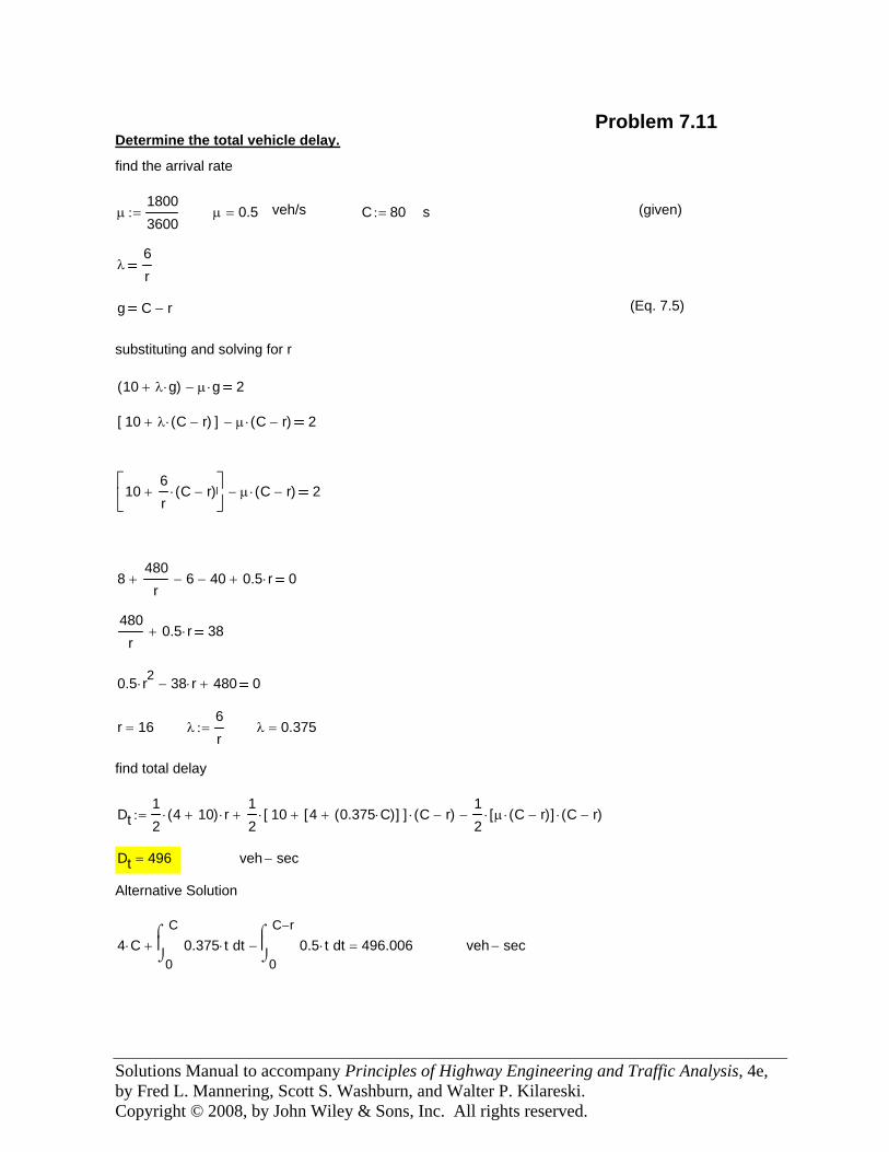
Solutions Manual to accompany Principles of Highway Engineering and Traffic Analysis, 4e, by Fred L. Mannering, Scott S. Washburn, and Walter P. Kilareski. Copyright © 2008, by John Wiley & Sons, Inc. All rights reserved.
veh sec−4 C⋅0
Ct0.375 t⋅
⌠⎮⌡
d+0
C r−t0.5 t⋅
⌠⎮⌡
d− 496.006=
Alternative Solution
veh sec−Dt 496=
Dt12
4 10+( )⋅ r⋅12
10 4 0.375 C⋅( )+[ ]+[ ]⋅ C r−( )⋅+12
μ C r−( )⋅[ ]⋅ C r−( )⋅−:=
find total delay
λ 0.375=λ6r
:=r 16=
0.5 r2⋅ 38 r⋅− 480+ 0
480r
0.5 r⋅+ 38
8480
r+ 6− 40− 0.5 r⋅+ 0
106r
C r−( )⋅+⎡⎢⎣
⎤⎥⎦
μ C r−( )⋅− 2
10 λ C r−( )⋅+[ ] μ C r−( )⋅− 2
10 λ g⋅+( ) μ g⋅− 2
substituting and solving for r
(Eq. 7.5)g C r−
λ6r
(given)sC 80:=veh/sμ 0.5=μ18003600
:=
find the arrival rate
Determine the total vehicle delay.Problem 7.11
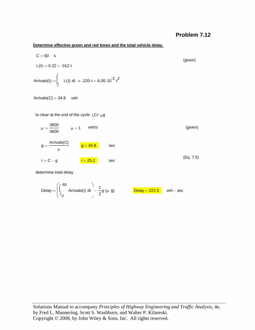
Solutions Manual to accompany Principles of Highway Engineering and Traffic Analysis, 4e, by Fred L. Mannering, Scott S. Washburn, and Walter P. Kilareski. Copyright © 2008, by John Wiley & Sons, Inc. All rights reserved.
veh sec−Delay 222.5=Delay0
60tArrivals t( )
⌠⎮⌡
d⎛⎜⎜⎝
⎞⎟⎟⎠
12
g μ g⋅( )⋅−:=
determine total delay
secr 25.2=r C g−:=(Eq. 7.5)
secg 34.8=gArrivals C( )
μ:=
(given)veh/sμ 1=μ36003600
:=
to clear at the end of the cycle λC= μg
vehArrivals C( ) 34.8=
Arrivals t( ) tλ t( )⌠⎮⎮⌡
d .220 t⋅ 6.00 10-3⋅ t2⋅+→:=
λ t( ) 0.22 .012 t⋅+:=(given)
sC 60:=
Determine effective green and red times and the total vehicle delay.
Problem 7.12
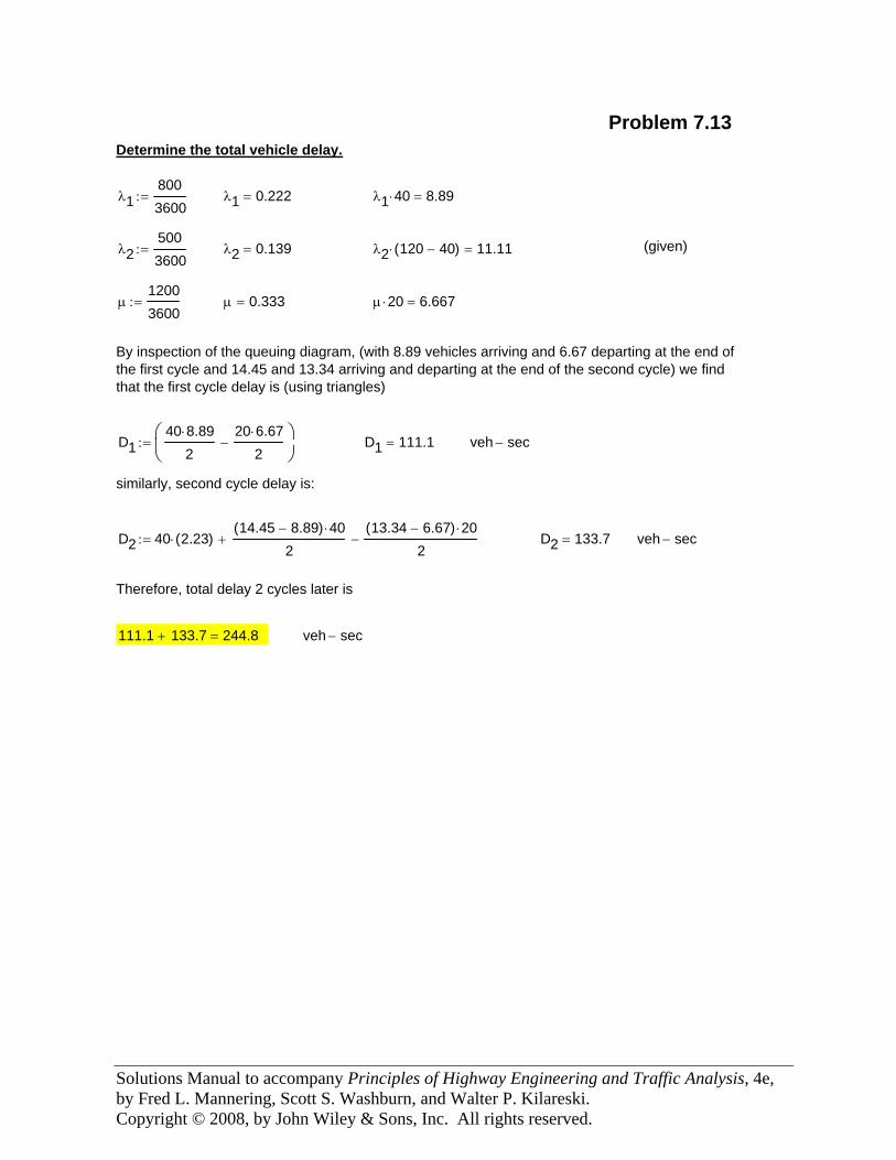
Solutions Manual to accompany Principles of Highway Engineering and Traffic Analysis, 4e, by Fred L. Mannering, Scott S. Washburn, and Walter P. Kilareski. Copyright © 2008, by John Wiley & Sons, Inc. All rights reserved.
veh sec−111.1 133.7+ 244.8=
Therefore, total delay 2 cycles later is
veh sec−D2 133.7=D2 40 2.23( )⋅14.45 8.89−( ) 40⋅
2+
13.34 6.67−( ) 20⋅
2−:=
similarly, second cycle delay is:
veh sec−D1 111.1=D140 8.89⋅
220 6.67⋅
2−
⎛⎜⎝
⎞⎟⎠
:=
By inspection of the queuing diagram, (with 8.89 vehicles arriving and 6.67 departing at the end of the first cycle and 14.45 and 13.34 arriving and departing at the end of the second cycle) we find that the first cycle delay is (using triangles)
μ 20⋅ 6.667=μ 0.333=μ12003600
:=
(given)λ2 120 40−( )⋅ 11.11=λ2 0.139=λ25003600
:=
λ1 40⋅ 8.89=λ1 0.222=λ18003600
:=
Determine the total vehicle delay.
Problem 7.13
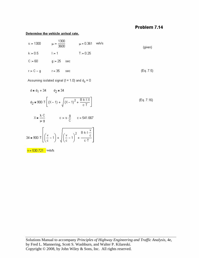
Solutions Manual to accompany Principles of Highway Engineering and Traffic Analysis, 4e, by Fred L. Mannering, Scott S. Washburn, and Walter P. Kilareski. Copyright © 2008, by John Wiley & Sons, Inc. All rights reserved.
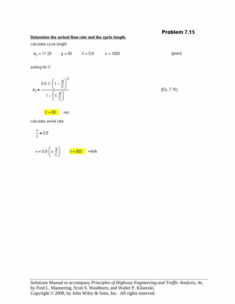
Solutions Manual to accompany Principles of Highway Engineering and Traffic Analysis, 4e, by Fred L. Mannering, Scott S. Washburn, and Walter P. Kilareski. Copyright © 2008, by John Wiley & Sons, Inc. All rights reserved.
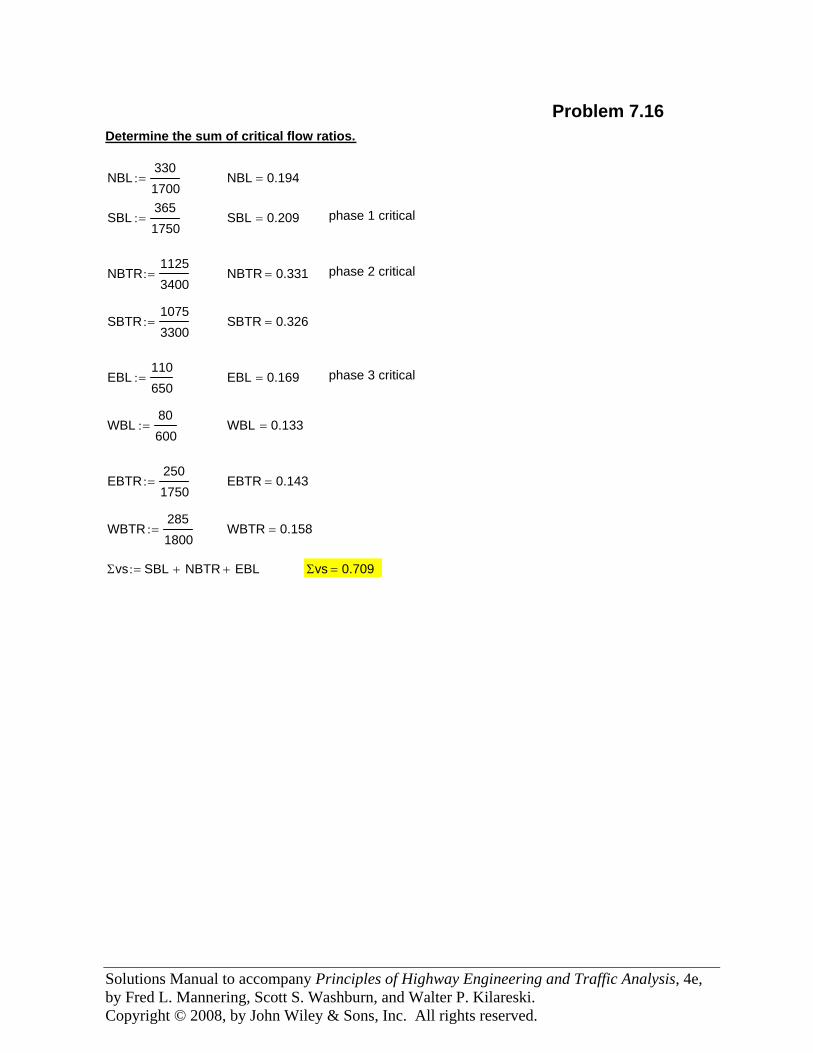
Solutions Manual to accompany Principles of Highway Engineering and Traffic Analysis, 4e, by Fred L. Mannering, Scott S. Washburn, and Walter P. Kilareski. Copyright © 2008, by John Wiley & Sons, Inc. All rights reserved.
Σvs 0.709=Σvs SBL NBTR+ EBL+:=
WBTR 0.158=WBTR2851800
:=
EBTR 0.143=EBTR2501750
:=
WBL 0.133=WBL80600
:=
phase 3 critical EBL 0.169=EBL110650
:=
SBTR 0.326=SBTR10753300
:=
phase 2 critical NBTR 0.331=NBTR11253400
:=
phase 1 critical SBL 0.209=SBL3651750
:=
NBL 0.194=NBL3301700
:=
Determine the sum of critical flow ratios.
Problem 7.16
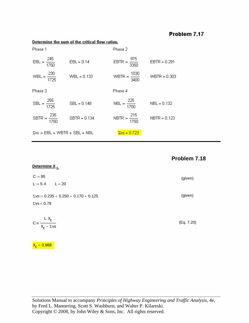
Solutions Manual to accompany Principles of Highway Engineering and Traffic Analysis, 4e, by Fred L. Mannering, Scott S. Washburn, and Walter P. Kilareski. Copyright © 2008, by John Wiley & Sons, Inc. All rights reserved.
Problem 7.18Determine X c.
C 95:= (given)L 5 4⋅:= L 20=
Σvs 0.235 0.250+ 0.170+ 0.125+:= (given)
Σvs 0.78=
CL Xc⋅
Xc Σvs−(Eq. 7.20)
Xc 0.988=
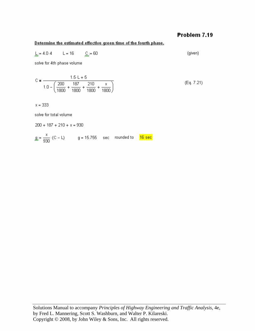
Solutions Manual to accompany Principles of Highway Engineering and Traffic Analysis, 4e, by Fred L. Mannering, Scott S. Washburn, and Walter P. Kilareski. Copyright © 2008, by John Wiley & Sons, Inc. All rights reserved.
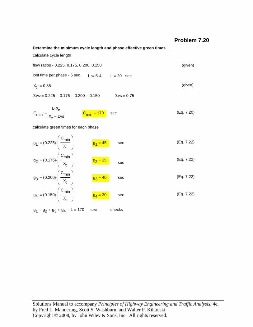
Solutions Manual to accompany Principles of Highway Engineering and Traffic Analysis, 4e, by Fred L. Mannering, Scott S. Washburn, and Walter P. Kilareski. Copyright © 2008, by John Wiley & Sons, Inc. All rights reserved.
g1 45= sec (Eq. 7.22)
g2 0.175( )Cmin
Xc
⎛⎜⎜⎝
⎞⎟⎟⎠
⋅:= g2 35= (Eq. 7.22)sec
g3 0.200( )Cmin
Xc
⎛⎜⎜⎝
⎞⎟⎟⎠
⋅:= g3 40= sec (Eq. 7.22)
g4 0.150( )Cmin
Xc
⎛⎜⎜⎝
⎞⎟⎟⎠
⋅:= g4 30= sec (Eq. 7.22)
g1 g2+ g3+ g4+ L+ 170= sec checks
Problem 7.20Determine the minimum cycle length and phase effective green times.
calculate cycle length
flow ratios - 0.225, 0.175, 0.200, 0.150 (given)
lost time per phase - 5 sec L 5 4⋅:= L 20= sec
Xc 0.85:= (given)
Σvs 0.225 0.175+ 0.200+ 0.150+:= Σvs 0.75=
CminL Xc⋅
Xc Σvs−:= Cmin 170= sec (Eq. 7.20)
calculate green times for each phase
g1 0.225( )Cmin
Xc
⎛⎜⎜⎝
⎞⎟⎟⎠
⋅:=
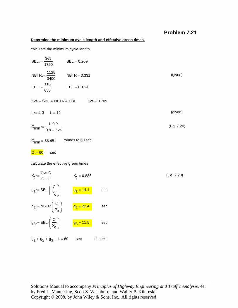
Solutions Manual to accompany Principles of Highway Engineering and Traffic Analysis, 4e, by Fred L. Mannering, Scott S. Washburn, and Walter P. Kilareski. Copyright © 2008, by John Wiley & Sons, Inc. All rights reserved.
C 60:= sec
calculate the effective green times
XcΣvs C⋅C L−
:= Xc 0.886= (Eq. 7.20)
g1 SBLCXc
⎛⎜⎝
⎞⎟⎠
⋅:= g1 14.1= sec
g2 NBTRCXc
⎛⎜⎝
⎞⎟⎠
⋅:= g2 22.4= sec
g3 EBLCXc
⎛⎜⎝
⎞⎟⎠
⋅:= g3 11.5= sec
g1 g2+ g3+ L+ 60= sec checks
Problem 7.21Determine the minimum cycle length and effective green times.
calculate the minimum cycle length
SBL3651750
:= SBL 0.209=
NBTR11253400
:= NBTR 0.331= (given)
EBL110650
:= EBL 0.169=
Σvs SBL NBTR+ EBL+:= Σvs 0.709=
L 4 3⋅:= L 12= (given)
CminL 0.9⋅
0.9 Σvs−:= (Eq. 7.20)
Cmin 56.451= rounds to 60 sec
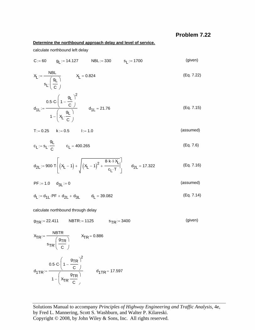
Solutions Manual to accompany Principles of Highway Engineering and Traffic Analysis, 4e, by Fred L. Mannering, Scott S. Washburn, and Walter P. Kilareski. Copyright © 2008, by John Wiley & Sons, Inc. All rights reserved.
(Eq. 7.6)
d2L 900 T⋅ XL 1−( ) XL 1−( )28 k⋅ I⋅ XL⋅
cL T⋅++
⎡⎢⎢⎣
⎤⎥⎥⎦
⋅:= d2L 17.322= (Eq. 7.16)
PF 1.0:= d3L 0:= (assumed)
dL d1L PF⋅ d2L+ d3L+:= dL 39.082= (Eq. 7.14)
calculate northbound through delay
gTR 22.411:= NBTR 1125:= sTR 3400:= (given)
XTRNBTR
sTRgTRC
⎛⎜⎝
⎞⎟⎠
⋅
:= XTR 0.886=
d1TR
0.5 C⋅ 1gTRC
−⎛⎜⎝
⎞⎟⎠
2
⋅
1 XTRgTRC
⋅⎛⎜⎝
⎞⎟⎠
−
:= d1TR 17.597=
Problem 7.22Determine the northbound approach delay and level of service.
calculate northbound left delay
C 60:= gL 14.127:= NBL 330:= sL 1700:= (given)
XLNBL
sLgLC
⎛⎜⎝
⎞⎟⎠
⋅
:= XL 0.824= (Eq. 7.22)
d1L
0.5 C⋅ 1gLC
−⎛⎜⎝
⎞⎟⎠
2
⋅
1 XLgLC
⋅⎛⎜⎝
⎞⎟⎠
−
:= d1L 21.76= (Eq. 7.15)
T 0.25:= k 0.5:= I 1.0:= (assumed)
cL sLgLC
⋅:= cL 400.265=
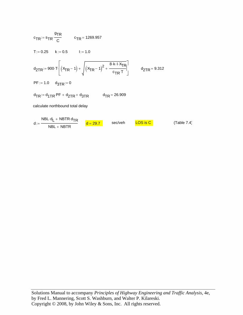
Solutions Manual to accompany Principles of Highway Engineering and Traffic Analysis, 4e, by Fred L. Mannering, Scott S. Washburn, and Walter P. Kilareski. Copyright © 2008, by John Wiley & Sons, Inc. All rights reserved.
(Table 7.4)LOS is C sec/vehd 29.7=dNBL dL⋅ NBTR dTR⋅+
NBL NBTR+:=
calculate northbound total delay
dTR 26.909=dTR d1TR PF⋅ d2TR+ d3TR+:=
d3TR 0:=PF 1.0:=
d2TR 9.312=d2TR 900 T⋅ XTR 1−( ) XTR 1−( )28 k⋅ I⋅ XTR⋅
cTR T⋅++
⎡⎢⎢⎣
⎤⎥⎥⎦
⋅:=
I 1.0:=k 0.5:=T 0.25:=
cTR 1269.957=cTR sTRgTRC
⋅:=

Solutions Manual to accompany Principles of Highway Engineering and Traffic Analysis, 4e, by Fred L. Mannering, Scott S. Washburn, and Walter P. Kilareski. Copyright © 2008, by John Wiley & Sons, Inc. All rights reserved.
(assumed)
d2L 900 T⋅ XL 1−( ) XL 1−( )28 k⋅ I⋅ XL⋅
cL T⋅++
⎡⎢⎢⎣
⎤⎥⎥⎦
⋅:= d2L 23.316= (Eq. 7.16)
PF 1.0:= d3L 0:= (assumed)
dL d1L PF⋅ d2L+ d3L+:= dL 45.474= (Eq. 7.14)
calculate southbound through and right delay
gTR 22.411:= SBTR 1075:= sTR 3300:= (given)
XTRSBTR
sTRgTRC
⎛⎜⎝
⎞⎟⎠
⋅
:= XTR 0.872=
d1TR
0.5 C⋅ 1gTRC
−⎛⎜⎝
⎞⎟⎠
2
⋅
1 XTRgTRC
⋅⎛⎜⎝
⎞⎟⎠
−
:= d1TR 17.463=
Problem 7.23Determine the southbound approach delay and level of service.
calculate southbound left delay
C 60:= gL 14.127:= SBL 365:= sL 1750:= (given)
XLSBL
sLgLC
⎛⎜⎝
⎞⎟⎠
⋅
:= XL 0.886= (Eq. 7.22)
d1L
0.5 C⋅ 1gLC
−⎛⎜⎝
⎞⎟⎠
2
⋅
1 XLgLC
⋅⎛⎜⎝
⎞⎟⎠
−
:= d1L 22.158= (Eq. 7.15)
cL sLgLC
⋅:= cL 412.038= (Eq. 7.6)
T 0.25:= k 0.5:= I 1.0:=
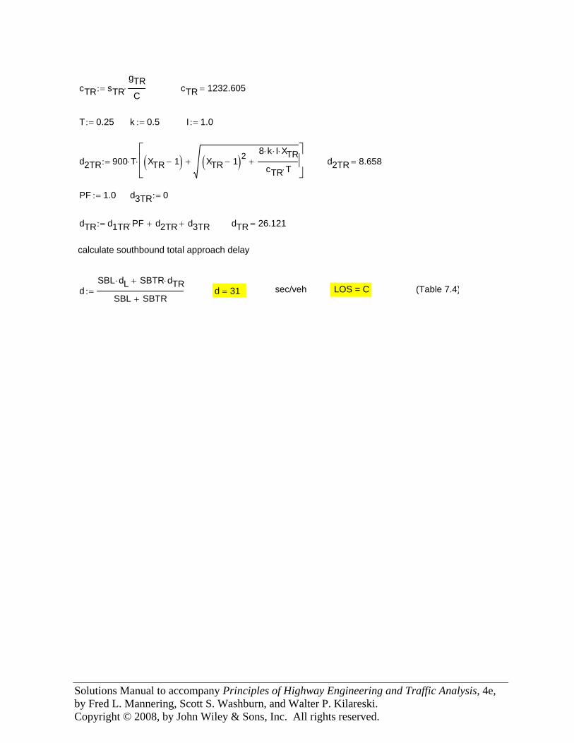
Solutions Manual to accompany Principles of Highway Engineering and Traffic Analysis, 4e, by Fred L. Mannering, Scott S. Washburn, and Walter P. Kilareski. Copyright © 2008, by John Wiley & Sons, Inc. All rights reserved.
(Table 7.4) LOS = Csec/vehd 31=dSBL dL⋅ SBTR dTR⋅+
SBL SBTR+:=
calculate southbound total approach delay
dTR 26.121=dTR d1TR PF⋅ d2TR+ d3TR+:=
d3TR 0:=PF 1.0:=
d2TR 8.658=d2TR 900 T⋅ XTR 1−( ) XTR 1−( )28 k⋅ I⋅ XTR⋅
cTR T⋅++
⎡⎢⎢⎣
⎤⎥⎥⎦
⋅:=
I 1.0:=k 0.5:=T 0.25:=
cTR 1232.605=cTR sTRgTRC
⋅:=
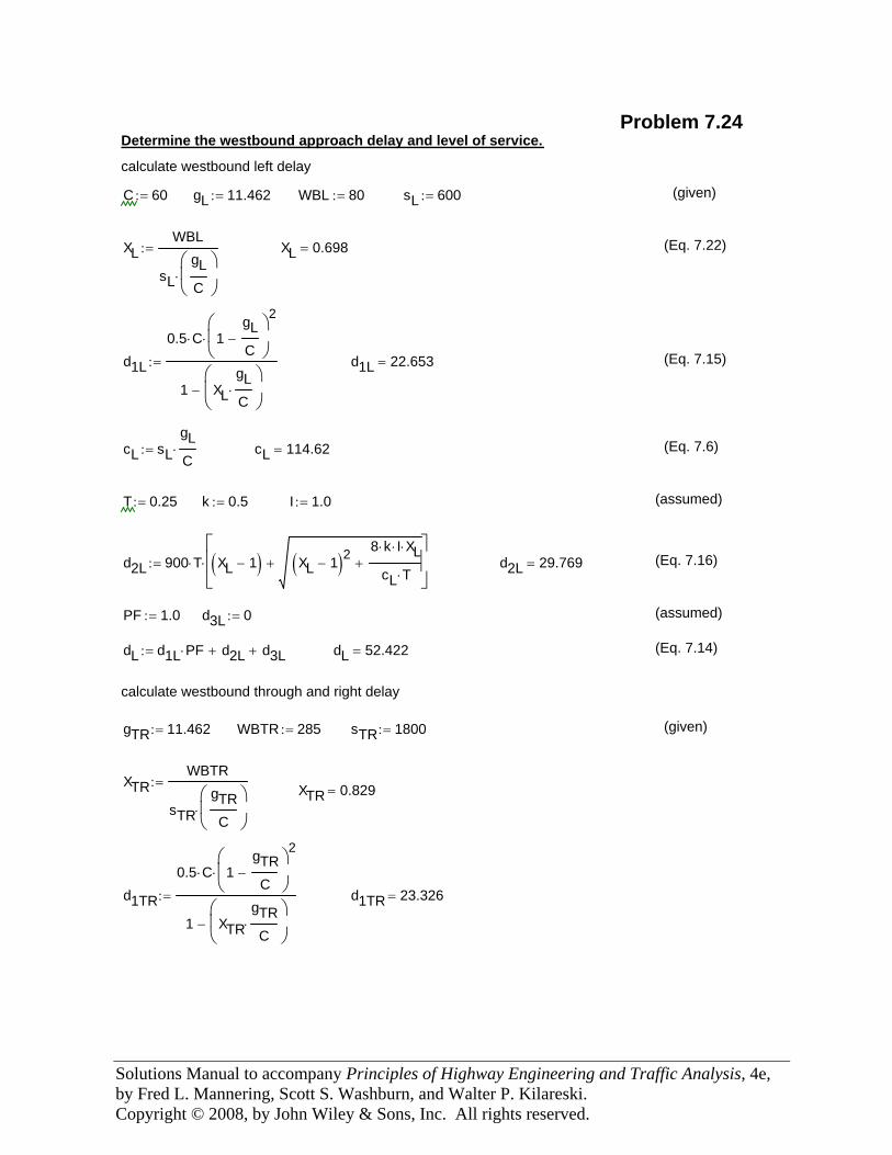
Solutions Manual to accompany Principles of Highway Engineering and Traffic Analysis, 4e, by Fred L. Mannering, Scott S. Washburn, and Walter P. Kilareski. Copyright © 2008, by John Wiley & Sons, Inc. All rights reserved.
Problem 7.24Determine the westbound approach delay and level of service.
calculate westbound left delay
C 60:= gL 11.462:= WBL 80:= sL 600:= (given)
XLWBL
sLgLC
⎛⎜⎝
⎞⎟⎠
⋅
:= XL 0.698= (Eq. 7.22)
d1L
0.5 C⋅ 1gLC
−⎛⎜⎝
⎞⎟⎠
2
⋅
1 XLgLC
⋅⎛⎜⎝
⎞⎟⎠
−
:= d1L 22.653= (Eq. 7.15)
cL sLgLC
⋅:= cL 114.62= (Eq. 7.6)
T 0.25:= k 0.5:= I 1.0:= (assumed)
d2L 900 T⋅ XL 1−( ) XL 1−( )28 k⋅ I⋅ XL⋅
cL T⋅++
⎡⎢⎢⎣
⎤⎥⎥⎦
⋅:= d2L 29.769= (Eq. 7.16)
PF 1.0:= d3L 0:= (assumed)
dL d1L PF⋅ d2L+ d3L+:= dL 52.422= (Eq. 7.14)
calculate westbound through and right delay
gTR 11.462:= WBTR 285:= sTR 1800:= (given)
XTRWBTR
sTRgTRC
⎛⎜⎝
⎞⎟⎠
⋅
:= XTR 0.829=
d1TR
0.5 C⋅ 1gTRC
−⎛⎜⎝
⎞⎟⎠
2
⋅
1 XTRgTRC
⋅⎛⎜⎝
⎞⎟⎠
−
:= d1TR 23.326=
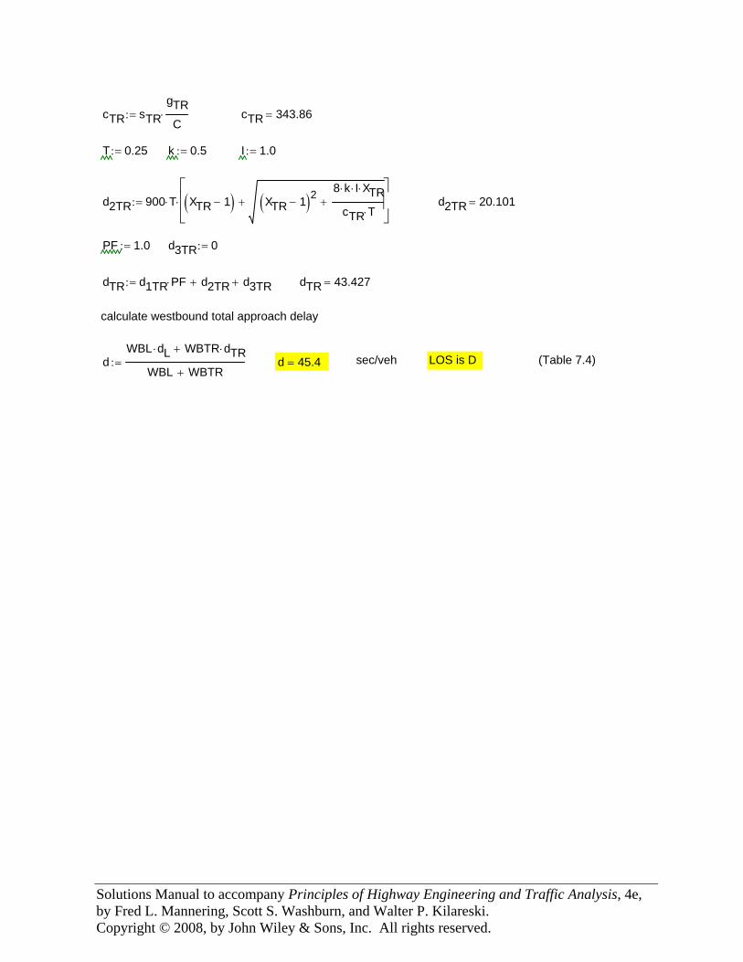
Solutions Manual to accompany Principles of Highway Engineering and Traffic Analysis, 4e, by Fred L. Mannering, Scott S. Washburn, and Walter P. Kilareski. Copyright © 2008, by John Wiley & Sons, Inc. All rights reserved.
cTR sTRgTRC
⋅:= cTR 343.86=
T 0.25:= k 0.5:= I 1.0:=
d2TR 900 T⋅ XTR 1−( ) XTR 1−( )28 k⋅ I⋅ XTR⋅
cTR T⋅++
⎡⎢⎢⎣
⎤⎥⎥⎦
⋅:= d2TR 20.101=
PF 1.0:= d3TR 0:=
dTR d1TR PF⋅ d2TR+ d3TR+:= dTR 43.427=
calculate westbound total approach delay
dWBL dL⋅ WBTR dTR⋅+
WBL WBTR+:= d 45.4= sec/veh LOS is D (Table 7.4)
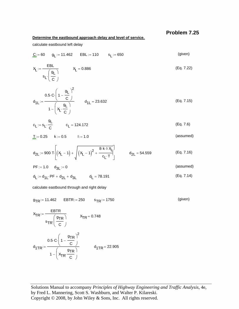
Solutions Manual to accompany Principles of Highway Engineering and Traffic Analysis, 4e, by Fred L. Mannering, Scott S. Washburn, and Walter P. Kilareski. Copyright © 2008, by John Wiley & Sons, Inc. All rights reserved.
Problem 7.25Determine the eastbound approach delay and level of service.
calculate eastbound left delay
C 60:= gL 11.462:= EBL 110:= sL 650:= (given)
XLEBL
sLgLC
⎛⎜⎝
⎞⎟⎠
⋅
:= XL 0.886= (Eq. 7.22)
d1L
0.5 C⋅ 1gLC
−⎛⎜⎝
⎞⎟⎠
2
⋅
1 XLgLC
⋅⎛⎜⎝
⎞⎟⎠
−
:= d1L 23.632= (Eq. 7.15)
cL sLgLC
⋅:= cL 124.172= (Eq. 7.6)
T 0.25:= k 0.5:= I 1.0:= (assumed)
d2L 900 T⋅ XL 1−( ) XL 1−( )28 k⋅ I⋅ XL⋅
cL T⋅++
⎡⎢⎢⎣
⎤⎥⎥⎦
⋅:= d2L 54.559= (Eq. 7.16)
PF 1.0:= d3L 0:= (assumed)
dL d1L PF⋅ d2L+ d3L+:= dL 78.191= (Eq. 7.14)
calculate eastbound through and right delay
gTR 11.462:= EBTR 250:= sTR 1750:= (given)
XTREBTR
sTRgTRC
⎛⎜⎝
⎞⎟⎠
⋅
:= XTR 0.748=
d1TR
0.5 C⋅ 1gTRC
−⎛⎜⎝
⎞⎟⎠
2
⋅
1 XTRgTRC
⋅⎛⎜⎝
⎞⎟⎠
−
:= d1TR 22.905=
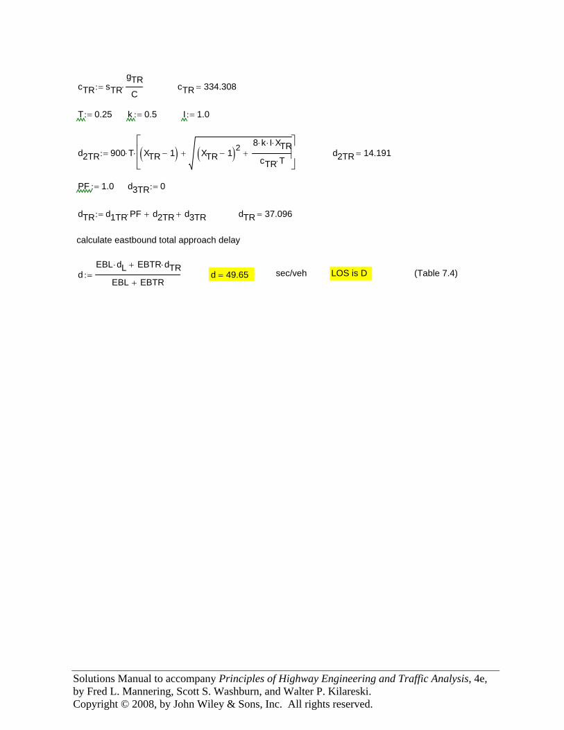
Solutions Manual to accompany Principles of Highway Engineering and Traffic Analysis, 4e, by Fred L. Mannering, Scott S. Washburn, and Walter P. Kilareski. Copyright © 2008, by John Wiley & Sons, Inc. All rights reserved.
cTR sTRgTRC
⋅:= cTR 334.308=
T 0.25:= k 0.5:= I 1.0:=
d2TR 900 T⋅ XTR 1−( ) XTR 1−( )28 k⋅ I⋅ XTR⋅
cTR T⋅++
⎡⎢⎢⎣
⎤⎥⎥⎦
⋅:= d2TR 14.191=
PF 1.0:= d3TR 0:=
dTR d1TR PF⋅ d2TR+ d3TR+:= dTR 37.096=
calculate eastbound total approach delay
dEBL dL⋅ EBTR dTR⋅+
EBL EBTR+:= d 49.65= sec/veh LOS is D (Table 7.4)
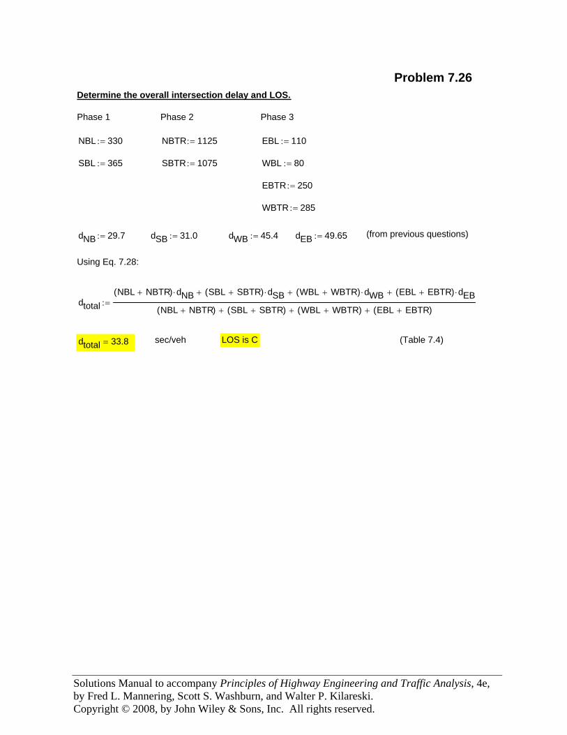
Solutions Manual to accompany Principles of Highway Engineering and Traffic Analysis, 4e, by Fred L. Mannering, Scott S. Washburn, and Walter P. Kilareski. Copyright © 2008, by John Wiley & Sons, Inc. All rights reserved.
Problem 7.26Determine the overall intersection delay and LOS.
Phase 1 Phase 2 Phase 3
NBL 330:= NBTR 1125:= EBL 110:=
SBL 365:= SBTR 1075:= WBL 80:=
EBTR 250:=
WBTR 285:=
dNB 29.7:= dSB 31.0:= dWB 45.4:= dEB 49.65:= (from previous questions)
Using Eq. 7.28:
dtotalNBL NBTR+( ) dNB⋅ SBL SBTR+( ) dSB⋅+ WBL WBTR+( ) dWB⋅+ EBL EBTR+( ) dEB⋅+
NBL NBTR+( ) SBL SBTR+( )+ WBL WBTR+( )+ EBL EBTR+( )+:=
dtotal 33.8= sec/veh LOS is C (Table 7.4)
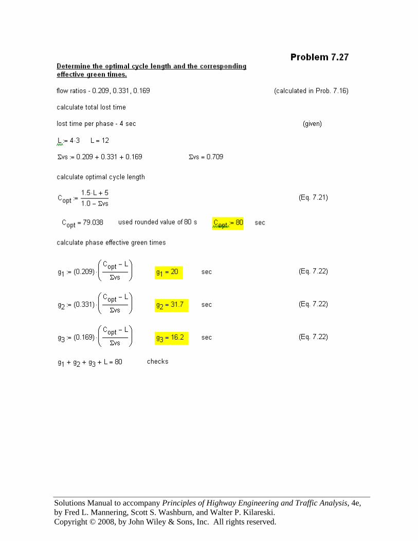
Solutions Manual to accompany Principles of Highway Engineering and Traffic Analysis, 4e, by Fred L. Mannering, Scott S. Washburn, and Walter P. Kilareski. Copyright © 2008, by John Wiley & Sons, Inc. All rights reserved.
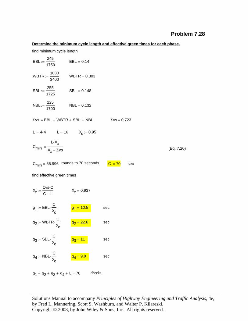
Solutions Manual to accompany Principles of Highway Engineering and Traffic Analysis, 4e, by Fred L. Mannering, Scott S. Washburn, and Walter P. Kilareski. Copyright © 2008, by John Wiley & Sons, Inc. All rights reserved.
C 70:= sec
find effective green times
XcΣvs C⋅C L−
:= Xc 0.937=
g1 EBLCXc⋅:= g1 10.5= sec
g2 WBTRCXc⋅:= g2 22.6= sec
g3 SBLCXc⋅:= g3 11= sec
g4 NBLCXc⋅:= g4 9.9= sec
g1 g2+ g3+ g4+ L+ 70= checks
Problem 7.28
Determine the minimum cycle length and effective green times for each phase.
find minimum cycle length
EBL2451750
:= EBL 0.14=
WBTR10303400
:= WBTR 0.303=
SBL2551725
:= SBL 0.148=
NBL2251700
:= NBL 0.132=
Σvs EBL WBTR+ SBL+ NBL+:= Σvs 0.723=
L 4 4⋅:= L 16= Xc 0.95:=
CminL Xc⋅
Xc Σvs−:= (Eq. 7.20)
Cmin 66.996= rounds to 70 seconds
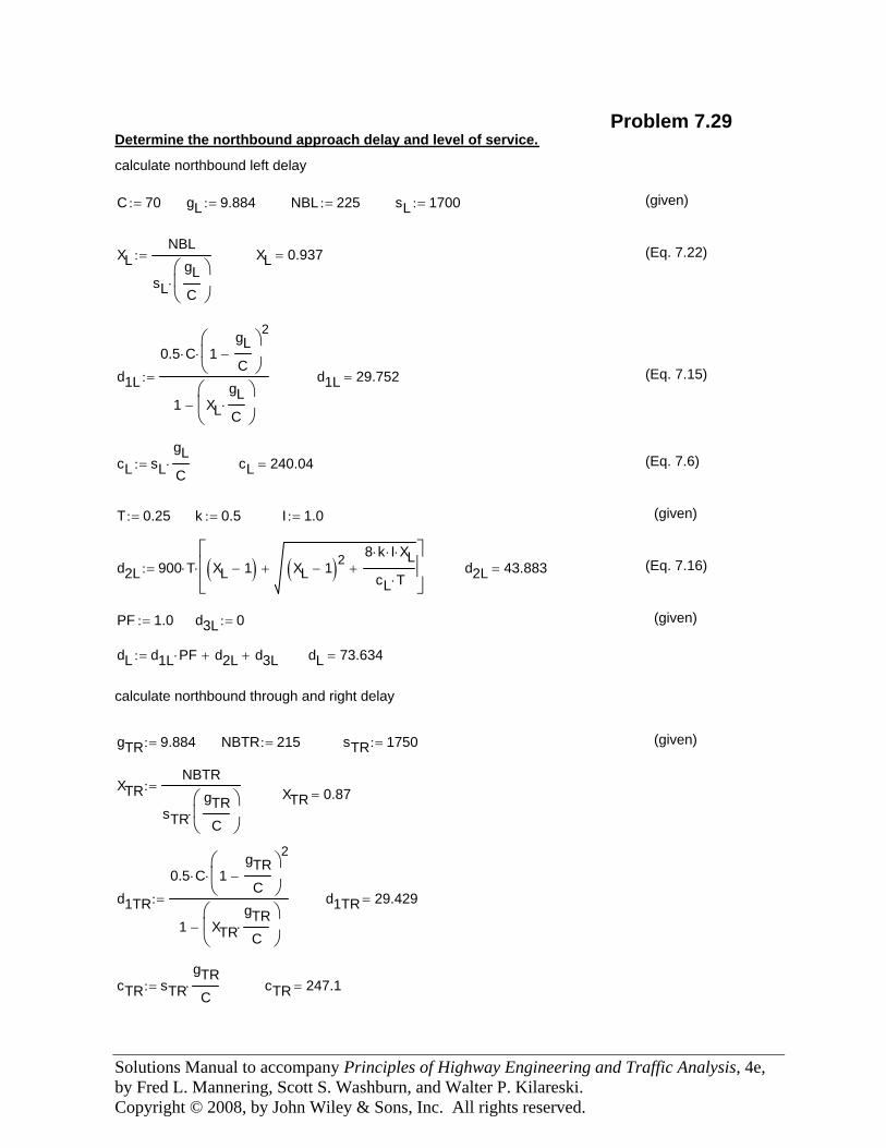
Solutions Manual to accompany Principles of Highway Engineering and Traffic Analysis, 4e, by Fred L. Mannering, Scott S. Washburn, and Walter P. Kilareski. Copyright © 2008, by John Wiley & Sons, Inc. All rights reserved.
(given)
d2L 900 T⋅ XL 1−( ) XL 1−( )28 k⋅ I⋅ XL⋅
cL T⋅++
⎡⎢⎢⎣
⎤⎥⎥⎦
⋅:= d2L 43.883= (Eq. 7.16)
PF 1.0:= d3L 0:= (given)
dL d1L PF⋅ d2L+ d3L+:= dL 73.634=
calculate northbound through and right delay
gTR 9.884:= NBTR 215:= sTR 1750:= (given)
XTRNBTR
sTRgTRC
⎛⎜⎝
⎞⎟⎠
⋅
:= XTR 0.87=
d1TR
0.5 C⋅ 1gTRC
−⎛⎜⎝
⎞⎟⎠
2
⋅
1 XTRgTRC
⋅⎛⎜⎝
⎞⎟⎠
−
:= d1TR 29.429=
cTR sTRgTRC
⋅:= cTR 247.1=
Problem 7.29Determine the northbound approach delay and level of service.
calculate northbound left delay
C 70:= gL 9.884:= NBL 225:= sL 1700:= (given)
XLNBL
sLgLC
⎛⎜⎝
⎞⎟⎠
⋅
:= XL 0.937= (Eq. 7.22)
d1L
0.5 C⋅ 1gLC
−⎛⎜⎝
⎞⎟⎠
2
⋅
1 XLgLC
⋅⎛⎜⎝
⎞⎟⎠
−
:= d1L 29.752= (Eq. 7.15)
cL sLgLC
⋅:= cL 240.04= (Eq. 7.6)
T 0.25:= k 0.5:= I 1.0:=
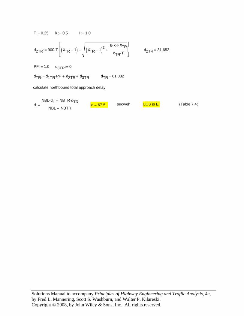
Solutions Manual to accompany Principles of Highway Engineering and Traffic Analysis, 4e, by Fred L. Mannering, Scott S. Washburn, and Walter P. Kilareski. Copyright © 2008, by John Wiley & Sons, Inc. All rights reserved.
T 0.25:= k 0.5:= I 1.0:=
d2TR 900 T⋅ XTR 1−( ) XTR 1−( )28 k⋅ I⋅ XTR⋅
cTR T⋅++
⎡⎢⎢⎣
⎤⎥⎥⎦
⋅:= d2TR 31.652=
PF 1.0:= d3TR 0:=
dTR d1TR PF⋅ d2TR+ d3TR+:= dTR 61.082=
calculate northbound total approach delay
dNBL dL⋅ NBTR dTR⋅+
NBL NBTR+:= d 67.5= sec/veh LOS is E (Table 7.4)
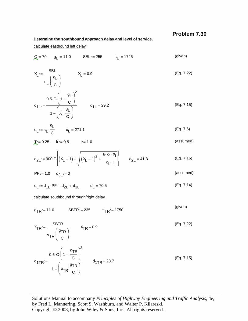
Solutions Manual to accompany Principles of Highway Engineering and Traffic Analysis, 4e, by Fred L. Mannering, Scott S. Washburn, and Walter P. Kilareski. Copyright © 2008, by John Wiley & Sons, Inc. All rights reserved.
Problem 7.30Determine the southbound approach delay and level of service.
calculate eastbound left delay
C 70:= gL 11.0:= SBL 255:= sL 1725:= (given)
XLSBL
sLgLC
⎛⎜⎝
⎞⎟⎠
⋅
:= XL 0.9= (Eq. 7.22)
d1L
0.5 C⋅ 1gLC
−⎛⎜⎝
⎞⎟⎠
2
⋅
1 XLgLC
⋅⎛⎜⎝
⎞⎟⎠
−
:= d1L 29.2= (Eq. 7.15)
cL sLgLC
⋅:= cL 271.1= (Eq. 7.6)
T 0.25:= k 0.5:= I 1.0:= (assumed)
d2L 900 T⋅ XL 1−( ) XL 1−( )28 k⋅ I⋅ XL⋅
cL T⋅++
⎡⎢⎢⎣
⎤⎥⎥⎦
⋅:= d2L 41.3= (Eq. 7.16)
PF 1.0:= d3L 0:= (assumed)
dL d1L PF⋅ d2L+ d3L+:= dL 70.5= (Eq. 7.14)
calculate southbound through/right delay
(given)gTR 11.0:= SBTR 235:= sTR 1750:=
(Eq. 7.22)XTR
SBTR
sTRgTRC
⎛⎜⎝
⎞⎟⎠
⋅
:= XTR 0.9=
(Eq. 7.15)d1TR
0.5 C⋅ 1gTRC
−⎛⎜⎝
⎞⎟⎠
2
⋅
1 XTRgTRC
⋅⎛⎜⎝
⎞⎟⎠
−
:= d1TR 28.7=
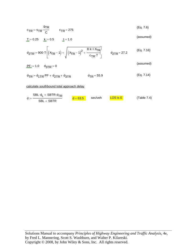
Solutions Manual to accompany Principles of Highway Engineering and Traffic Analysis, 4e, by Fred L. Mannering, Scott S. Washburn, and Walter P. Kilareski. Copyright © 2008, by John Wiley & Sons, Inc. All rights reserved.
(Eq. 7.6)cTR sTR
gTRC
⋅:= cTR 275=
(assumed)T 0.25:= k 0.5:= I 1.0:=
(Eq. 7.16)d2TR 900 T⋅ XTR 1−( ) XTR 1−( )2
8 k⋅ I⋅ XTR⋅
cTR T⋅++
⎡⎢⎢⎣
⎤⎥⎥⎦
⋅:= d2TR 27.2=
(assumed)PF 1.0:= d3TR 0:=
dTR d1TR PF⋅ d2TR+ d3TR+:= dTR 55.9= (Eq. 7.14)
calculate southbound total approach delay
dSBL dL⋅ SBTR dTR⋅+
SBL SBTR+:= d 63.5= sec/veh LOS is E (Table 7.4)
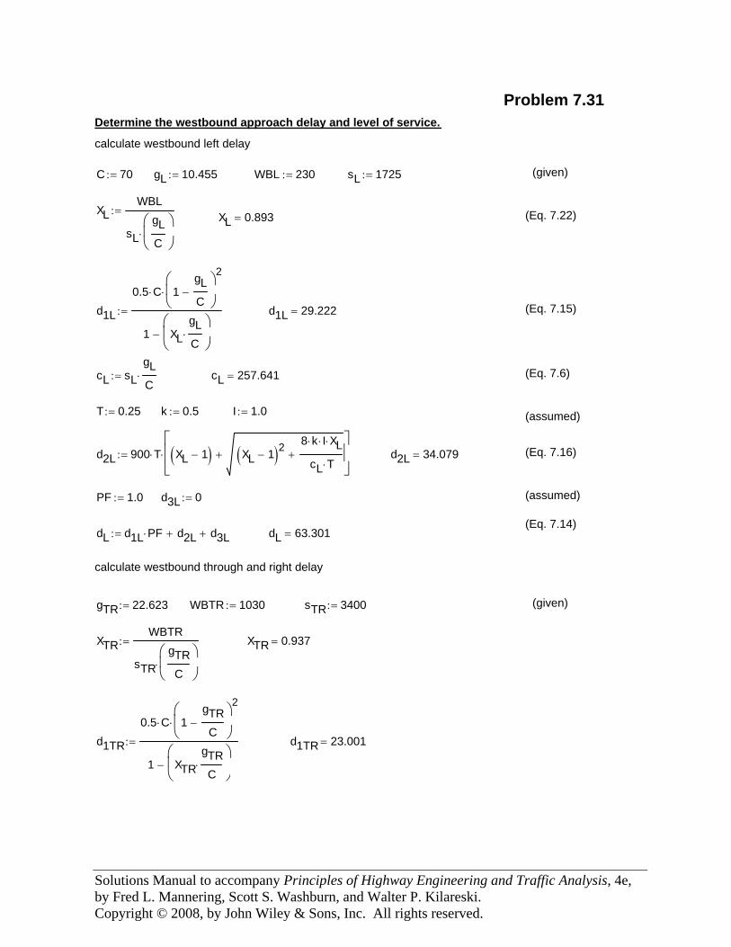
Solutions Manual to accompany Principles of Highway Engineering and Traffic Analysis, 4e, by Fred L. Mannering, Scott S. Washburn, and Walter P. Kilareski. Copyright © 2008, by John Wiley & Sons, Inc. All rights reserved.
(assumed)
d2L 900 T⋅ XL 1−( ) XL 1−( )28 k⋅ I⋅ XL⋅
cL T⋅++
⎡⎢⎢⎣
⎤⎥⎥⎦
⋅:= d2L 34.079= (Eq. 7.16)
PF 1.0:= d3L 0:= (assumed)
(Eq. 7.14)dL d1L PF⋅ d2L+ d3L+:= dL 63.301=
calculate westbound through and right delay
gTR 22.623:= WBTR 1030:= sTR 3400:= (given)
XTRWBTR
sTRgTRC
⎛⎜⎝
⎞⎟⎠
⋅
:= XTR 0.937=
d1TR
0.5 C⋅ 1gTRC
−⎛⎜⎝
⎞⎟⎠
2
⋅
1 XTRgTRC
⋅⎛⎜⎝
⎞⎟⎠
−
:= d1TR 23.001=
Problem 7.31Determine the westbound approach delay and level of service.
calculate westbound left delay
C 70:= gL 10.455:= WBL 230:= sL 1725:= (given)
XLWBL
sLgLC
⎛⎜⎝
⎞⎟⎠
⋅
:= XL 0.893= (Eq. 7.22)
d1L
0.5 C⋅ 1gLC
−⎛⎜⎝
⎞⎟⎠
2
⋅
1 XLgLC
⋅⎛⎜⎝
⎞⎟⎠
−
:= d1L 29.222= (Eq. 7.15)
cL sLgLC
⋅:= cL 257.641= (Eq. 7.6)
T 0.25:= k 0.5:= I 1.0:=
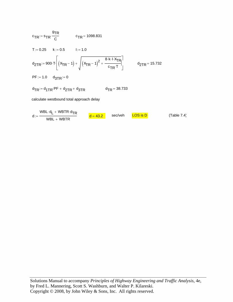
Solutions Manual to accompany Principles of Highway Engineering and Traffic Analysis, 4e, by Fred L. Mannering, Scott S. Washburn, and Walter P. Kilareski. Copyright © 2008, by John Wiley & Sons, Inc. All rights reserved.
(Table 7.4)LOS is Dsec/vehd 43.2=dWBL dL⋅ WBTR dTR⋅+
WBL WBTR+:=
calculate westbound total approach delay
dTR 38.733=dTR d1TR PF⋅ d2TR+ d3TR+:=
d3TR 0:=PF 1.0:=
d2TR 15.732=d2TR 900 T⋅ XTR 1−( ) XTR 1−( )28 k⋅ I⋅ XTR⋅
cTR T⋅++
⎡⎢⎢⎣
⎤⎥⎥⎦
⋅:=
I 1.0:=k 0.5:=T 0.25:=
cTR 1098.831=cTR sTRgTRC
⋅:=
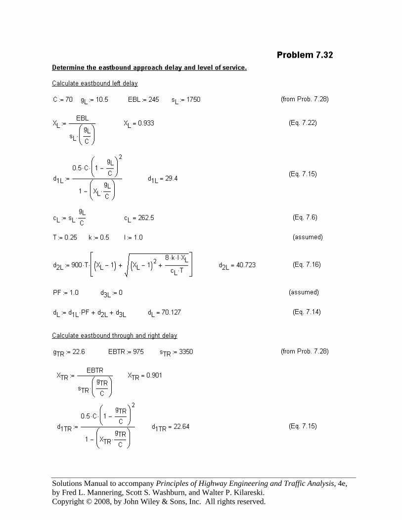
Solutions Manual to accompany Principles of Highway Engineering and Traffic Analysis, 4e, by Fred L. Mannering, Scott S. Washburn, and Walter P. Kilareski. Copyright © 2008, by John Wiley & Sons, Inc. All rights reserved.
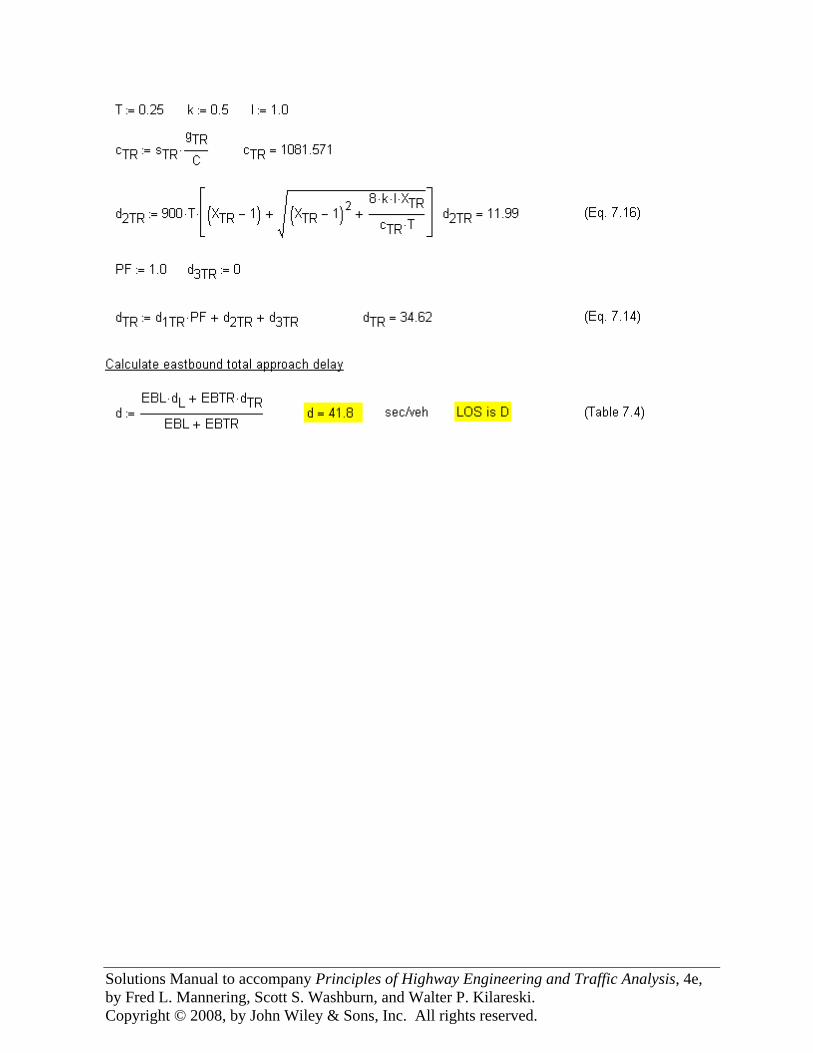
Solutions Manual to accompany Principles of Highway Engineering and Traffic Analysis, 4e, by Fred L. Mannering, Scott S. Washburn, and Walter P. Kilareski. Copyright © 2008, by John Wiley & Sons, Inc. All rights reserved.
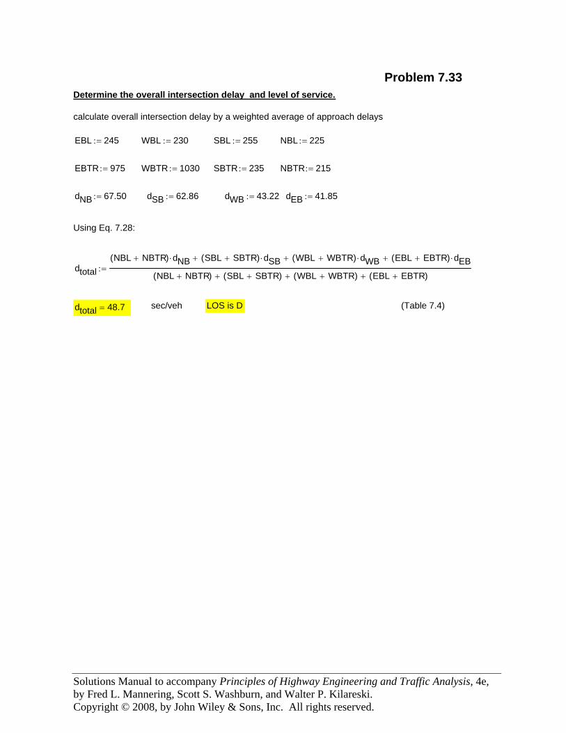
Solutions Manual to accompany Principles of Highway Engineering and Traffic Analysis, 4e, by Fred L. Mannering, Scott S. Washburn, and Walter P. Kilareski. Copyright © 2008, by John Wiley & Sons, Inc. All rights reserved.
(Table 7.4)LOS is Dsec/vehdtotal 48.7=
dtotalNBL NBTR+( ) dNB⋅ SBL SBTR+( ) dSB⋅+ WBL WBTR+( ) dWB⋅+ EBL EBTR+( ) dEB⋅+
NBL NBTR+( ) SBL SBTR+( )+ WBL WBTR+( )+ EBL EBTR+( )+:=
Using Eq. 7.28:
dEB 41.85:=dWB 43.22:=dSB 62.86:=dNB 67.50:=
NBTR 215:=SBTR 235:=WBTR 1030:=EBTR 975:=
NBL 225:=SBL 255:=WBL 230:=EBL 245:=
calculate overall intersection delay by a weighted average of approach delays
Determine the overall intersection delay and level of service.
Problem 7.33
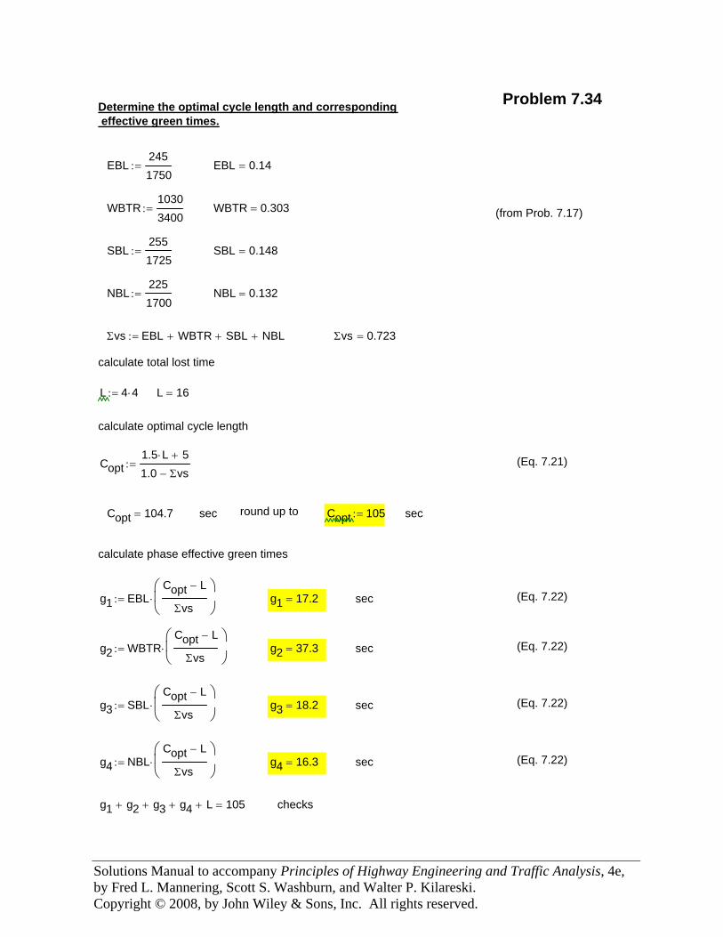
Solutions Manual to accompany Principles of Highway Engineering and Traffic Analysis, 4e, by Fred L. Mannering, Scott S. Washburn, and Walter P. Kilareski. Copyright © 2008, by John Wiley & Sons, Inc. All rights reserved.
Problem 7.34Determine the optimal cycle length and corresponding effective green times.
EBL2451750
:= EBL 0.14=
WBTR10303400
:= WBTR 0.303= (from Prob. 7.17)
SBL2551725
:= SBL 0.148=
NBL2251700
:= NBL 0.132=
Σvs EBL WBTR+ SBL+ NBL+:= Σvs 0.723=
calculate total lost time
L 4 4⋅:= L 16=
calculate optimal cycle length
Copt1.5 L⋅ 5+
1.0 Σvs−:= (Eq. 7.21)
Copt 104.7= sec round up to Copt 105:= sec
calculate phase effective green times
g1 EBLCopt L−
Σvs
⎛⎜⎝
⎞⎟⎠
⋅:= g1 17.2= sec (Eq. 7.22)
g2 WBTRCopt L−
Σvs
⎛⎜⎝
⎞⎟⎠
⋅:= g2 37.3= sec (Eq. 7.22)
g3 SBLCopt L−
Σvs
⎛⎜⎝
⎞⎟⎠
⋅:= g3 18.2= sec (Eq. 7.22)
g4 NBLCopt L−
Σvs
⎛⎜⎝
⎞⎟⎠
⋅:= g4 16.3= sec (Eq. 7.22)
g1 g2+ g3+ g4+ L+ 105= checks
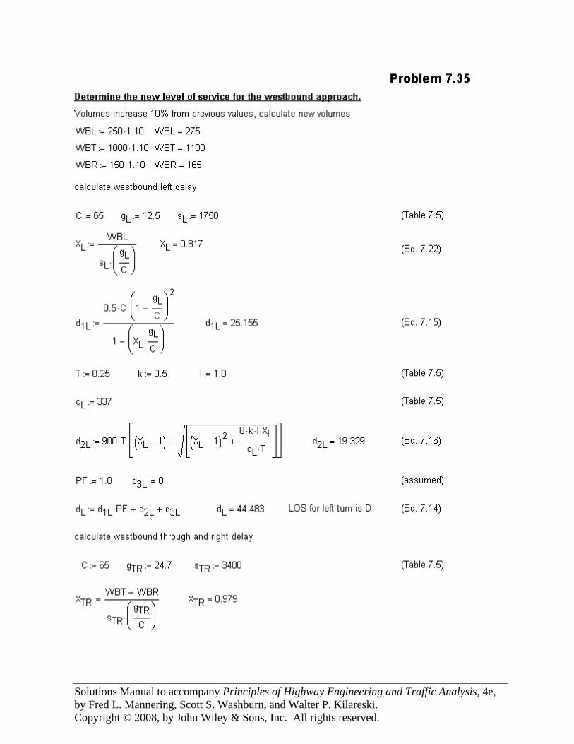
Solutions Manual to accompany Principles of Highway Engineering and Traffic Analysis, 4e, by Fred L. Mannering, Scott S. Washburn, and Walter P. Kilareski. Copyright © 2008, by John Wiley & Sons, Inc. All rights reserved.
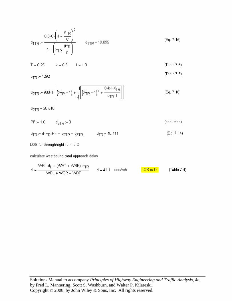
Solutions Manual to accompany Principles of Highway Engineering and Traffic Analysis, 4e, by Fred L. Mannering, Scott S. Washburn, and Walter P. Kilareski. Copyright © 2008, by John Wiley & Sons, Inc. All rights reserved.
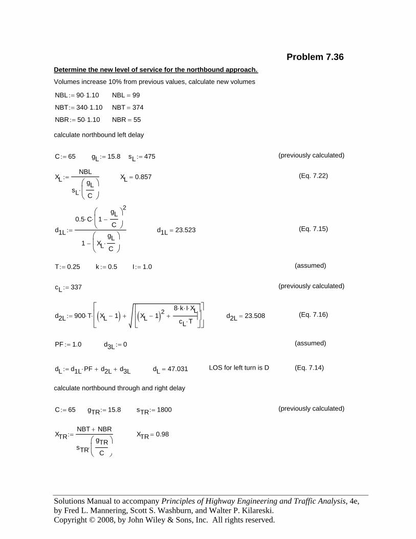
Solutions Manual to accompany Principles of Highway Engineering and Traffic Analysis, 4e, by Fred L. Mannering, Scott S. Washburn, and Walter P. Kilareski. Copyright © 2008, by John Wiley & Sons, Inc. All rights reserved.
I 1.0:= (assumed)
cL 337:= (previously calculated)
d2L 900 T⋅ XL 1−( ) XL 1−( )28 k⋅ I⋅ XL⋅
cL T⋅+
⎡⎢⎢⎣
⎤⎥⎥⎦
+⎡⎢⎢⎣
⎤⎥⎥⎦
⋅:= d2L 23.508= (Eq. 7.16)
PF 1.0:= d3L 0:= (assumed)
dL d1L PF⋅ d2L+ d3L+:= dL 47.031= LOS for left turn is D (Eq. 7.14)
calculate northbound through and right delay
C 65:= gTR 15.8:= sTR 1800:= (previously calculated)
XTRNBT NBR+
sTRgTRC
⎛⎜⎝
⎞⎟⎠
⋅
:= XTR 0.98=
Problem 7.36Determine the new level of service for the northbound approach.
Volumes increase 10% from previous values, calculate new volumes
NBL 90 1.10⋅:= NBL 99=
NBT 340 1.10⋅:= NBT 374=
NBR 50 1.10⋅:= NBR 55=
calculate northbound left delay
C 65:= gL 15.8:= sL 475:= (previously calculated)
XLNBL
sLgLC
⎛⎜⎝
⎞⎟⎠
⋅
:= XL 0.857= (Eq. 7.22)
d1L
0.5 C⋅ 1gLC
−⎛⎜⎝
⎞⎟⎠
2
⋅
1 XLgLC
⋅⎛⎜⎝
⎞⎟⎠
−
:= d1L 23.523= (Eq. 7.15)
T 0.25:= k 0.5:=
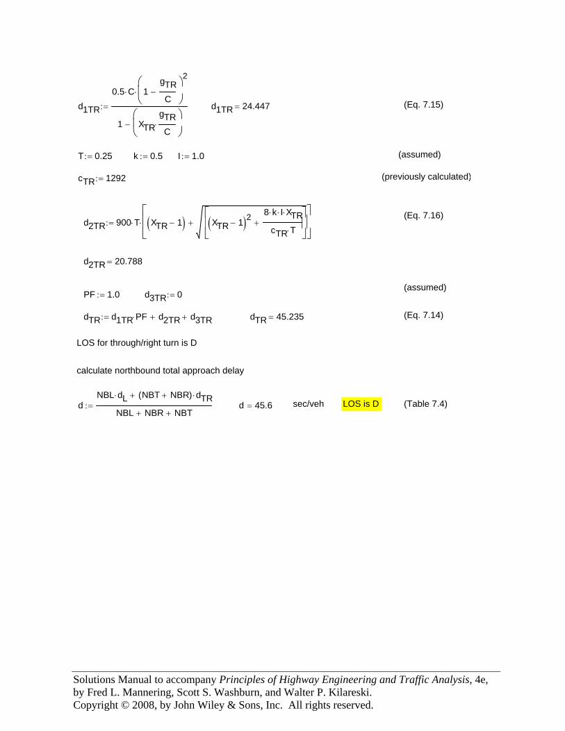
Solutions Manual to accompany Principles of Highway Engineering and Traffic Analysis, 4e, by Fred L. Mannering, Scott S. Washburn, and Walter P. Kilareski. Copyright © 2008, by John Wiley & Sons, Inc. All rights reserved.
(Table 7.4)LOS is Dsec/vehd 45.6=dNBL dL⋅ NBT NBR+( ) dTR⋅+
NBL NBR+ NBT+:=
calculate northbound total approach delay
LOS for through/right turn is D
(Eq. 7.14)dTR 45.235=dTR d1TR PF⋅ d2TR+ d3TR+:=
d3TR 0:=PF 1.0:=(assumed)
d2TR 20.788=
d2TR 900 T⋅ XTR 1−( ) XTR 1−( )28 k⋅ I⋅ XTR⋅
cTR T⋅+
⎡⎢⎢⎣
⎤⎥⎥⎦
+⎡⎢⎢⎣
⎤⎥⎥⎦
⋅:=(Eq. 7.16)
(previously calculated)cTR 1292:=
(assumed) I 1.0:=k 0.5:=T 0.25:=
(Eq. 7.15)d1TR 24.447=d1TR
0.5 C⋅ 1gTRC
−⎛⎜⎝
⎞⎟⎠
2
⋅
1 XTRgTRC
⋅⎛⎜⎝
⎞⎟⎠
−
:=
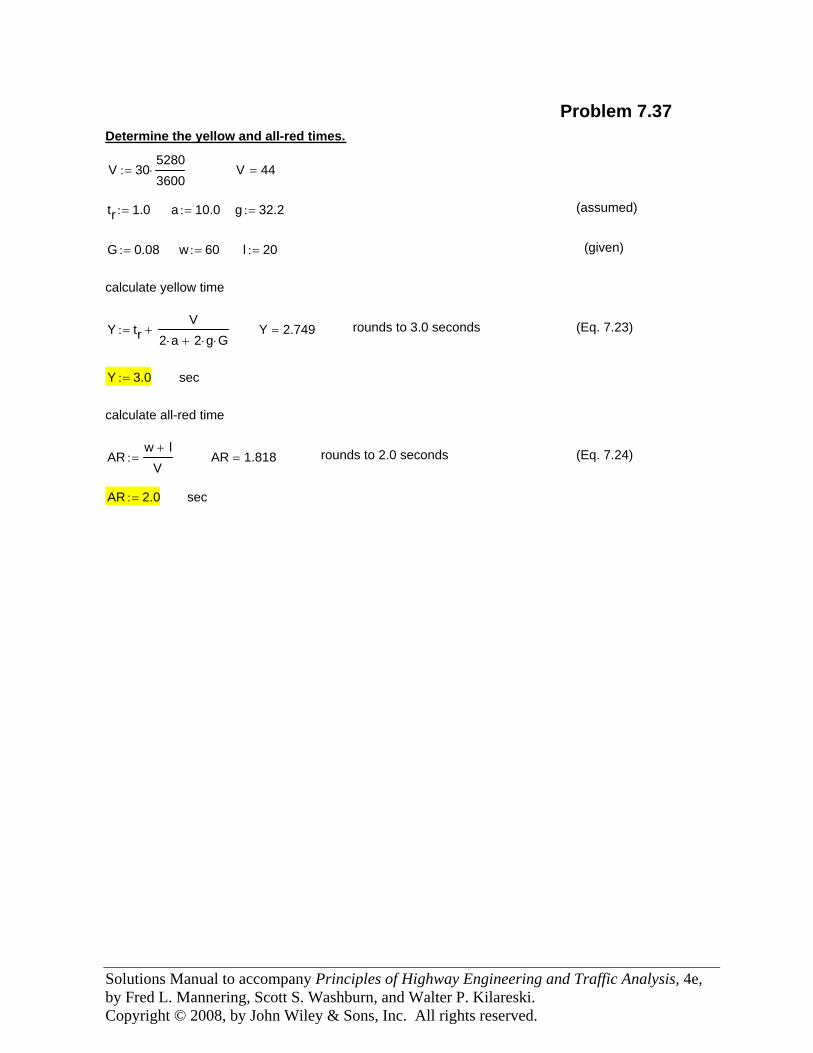
Solutions Manual to accompany Principles of Highway Engineering and Traffic Analysis, 4e, by Fred L. Mannering, Scott S. Washburn, and Walter P. Kilareski. Copyright © 2008, by John Wiley & Sons, Inc. All rights reserved.
secAR 2.0:=
(Eq. 7.24)rounds to 2.0 secondsAR 1.818=ARw l+
V:=
calculate all-red time
secY 3.0:=
(Eq. 7.23)rounds to 3.0 secondsY 2.749=Y trV
2 a⋅ 2 g⋅ G⋅++:=
calculate yellow time
(given) l 20:=w 60:=G 0.08:=
(assumed) g 32.2:=a 10.0:=tr 1.0:=
V 44=V 3052803600⋅:=
Determine the yellow and all-red times.
Problem 7.37
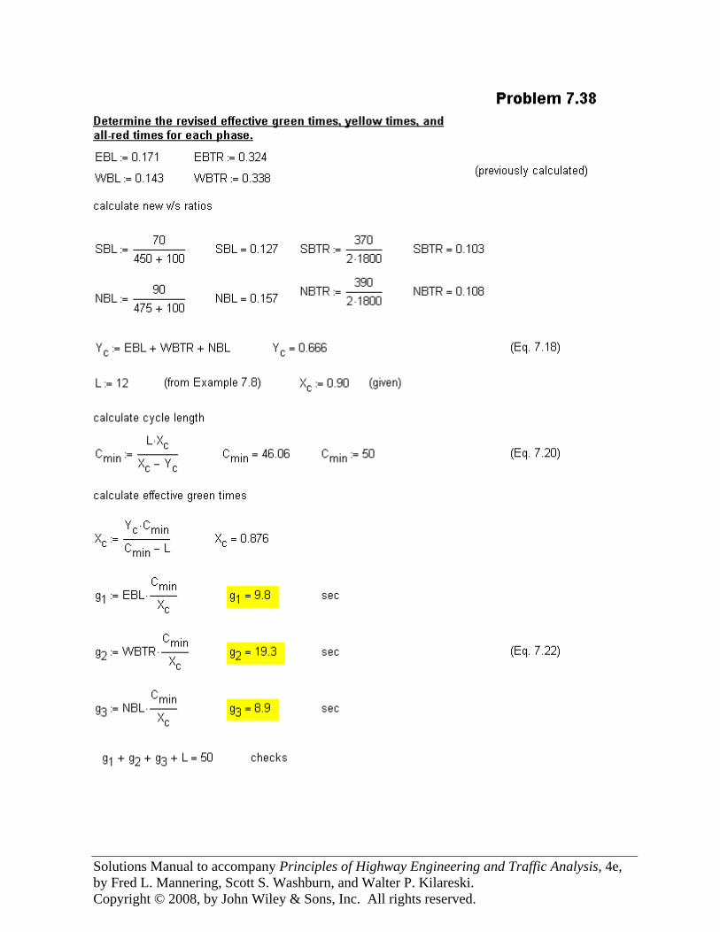
Solutions Manual to accompany Principles of Highway Engineering and Traffic Analysis, 4e, by Fred L. Mannering, Scott S. Washburn, and Walter P. Kilareski. Copyright © 2008, by John Wiley & Sons, Inc. All rights reserved.
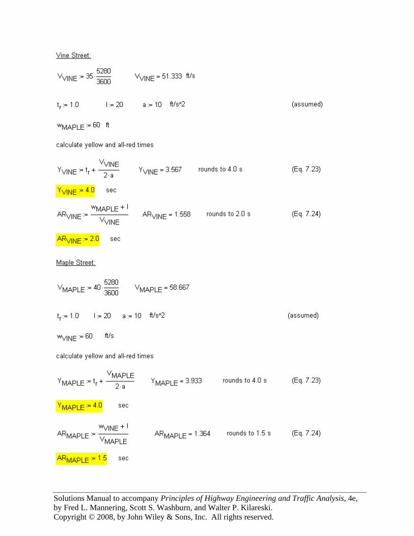
Solutions Manual to accompany Principles of Highway Engineering and Traffic Analysis, 4e, by Fred L. Mannering, Scott S. Washburn, and Walter P. Kilareski. Copyright © 2008, by John Wiley & Sons, Inc. All rights reserved.
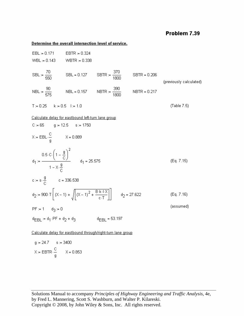
Solutions Manual to accompany Principles of Highway Engineering and Traffic Analysis, 4e, by Fred L. Mannering, Scott S. Washburn, and Walter P. Kilareski. Copyright © 2008, by John Wiley & Sons, Inc. All rights reserved.
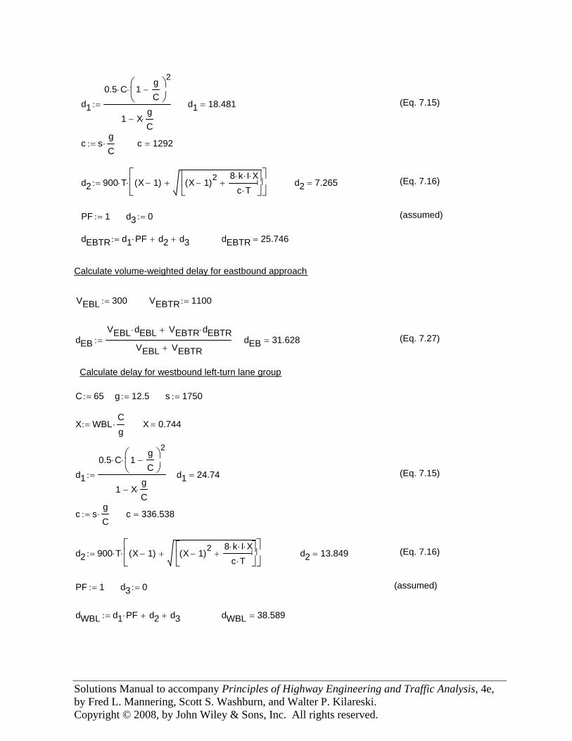
Solutions Manual to accompany Principles of Highway Engineering and Traffic Analysis, 4e, by Fred L. Mannering, Scott S. Washburn, and Walter P. Kilareski. Copyright © 2008, by John Wiley & Sons, Inc. All rights reserved.
Calculate delay for westbound left-turn lane group
C 65:= g 12.5:= s 1750:=
X WBLCg⋅:= X 0.744=
d1
0.5 C⋅ 1gC
−⎛⎜⎝
⎞⎟⎠
2⋅
1 XgC⋅−
:= d1 24.74= (Eq. 7.15)
c sgC⋅:= c 336.538=
d2 900 T⋅ X 1−( ) X 1−( )28 k⋅ I⋅ X⋅
c T⋅+
⎡⎢⎣
⎤⎥⎦
+⎡⎢⎣
⎤⎥⎦
⋅:= d2 13.849= (Eq. 7.16)
PF 1:= d3 0:= (assumed)
dWBL d1 PF⋅ d2+ d3+:= dWBL 38.589=
d1
0.5 C⋅ 1gC
−⎛⎜⎝
⎞⎟⎠
2⋅
1 XgC⋅−
:= d1 18.481= (Eq. 7.15)
c sgC⋅:= c 1292=
d2 900 T⋅ X 1−( ) X 1−( )28 k⋅ I⋅ X⋅
c T⋅+
⎡⎢⎣
⎤⎥⎦
+⎡⎢⎣
⎤⎥⎦
⋅:= d2 7.265= (Eq. 7.16)
PF 1:= d3 0:= (assumed)
dEBTR d1 PF⋅ d2+ d3+:= dEBTR 25.746=
Calculate volume-weighted delay for eastbound approach
VEBL 300:= VEBTR 1100:=
dEBVEBL dEBL⋅ VEBTR dEBTR⋅+
VEBL VEBTR+:= dEB 31.628= (Eq. 7.27)
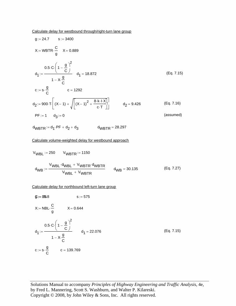
Solutions Manual to accompany Principles of Highway Engineering and Traffic Analysis, 4e, by Fred L. Mannering, Scott S. Washburn, and Walter P. Kilareski. Copyright © 2008, by John Wiley & Sons, Inc. All rights reserved.
Calculate volume-weighted delay for westbound approach
VWBL 250:= VWBTR 1150:=
dWBVWBL dWBL⋅ VWBTR dWBTR⋅+
VWBL VWBTR+:= dWB 30.135= (Eq. 7.27)
Calculate delay for northbound left-turn lane group
g 15.8:=C 65:= s 575:=
X NBLCg⋅:= X 0.644=
d1
0.5 C⋅ 1gC
−⎛⎜⎝
⎞⎟⎠
2⋅
1 XgC⋅−
:= d1 22.076= (Eq. 7.15)
c sgC⋅:= c 139.769=
Calculate delay for westbound through/right-turn lane group
g 24.7:= s 3400:=
X WBTRCg⋅:= X 0.889=
d1
0.5 C⋅ 1gC
−⎛⎜⎝
⎞⎟⎠
2⋅
1 XgC⋅−
:= d1 18.872= (Eq. 7.15)
c sgC⋅:= c 1292=
d2 900 T⋅ X 1−( ) X 1−( )28 k⋅ I⋅ X⋅
c T⋅+
⎡⎢⎣
⎤⎥⎦
+⎡⎢⎣
⎤⎥⎦
⋅:= d2 9.426= (Eq. 7.16)
PF 1:= d3 0:= (assumed)
dWBTR d1 PF⋅ d2+ d3+:= dWBTR 28.297=
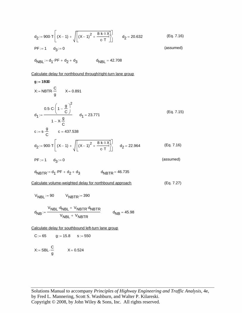
Solutions Manual to accompany Principles of Highway Engineering and Traffic Analysis, 4e, by Fred L. Mannering, Scott S. Washburn, and Walter P. Kilareski. Copyright © 2008, by John Wiley & Sons, Inc. All rights reserved.
d2 22.964= (Eq. 7.16)
PF 1:= d3 0:= (assumed)
dNBTR d1 PF⋅ d2+ d3+:= dNBTR 46.735=
Calculate volume-weighted delay for northbound approach (Eq. 7.27)
VNBL 90:= VNBTR 390:=
dNBVNBL dNBL⋅ VNBTR dNBTR⋅+
VNBL VNBTR+:= dNB 45.98=
Calculate delay for southbound left-turn lane group
C 65:= g 15.8:= s 550:=
X SBLCg⋅:= X 0.524=
d2 900 T⋅ X 1−( ) X 1−( )28 k⋅ I⋅ X⋅
c T⋅+
⎡⎢⎣
⎤⎥⎦
+⎡⎢⎣
⎤⎥⎦
⋅:= d2 20.632= (Eq. 7.16)
PF 1:= d3 0:= (assumed)
dNBL d1 PF⋅ d2+ d3+:= dNBL 42.708=
Calculate delay for northbound through/right-turn lane group
s 1800:=g 15.8:=
X NBTRCg⋅:= X 0.891=
(Eq. 7.15)d1
0.5 C⋅ 1gC
−⎛⎜⎝
⎞⎟⎠
2⋅
1 XgC⋅−
:= d1 23.771=
c sgC⋅:= c 437.538=
d2 900 T⋅ X 1−( ) X 1−( )28 k⋅ I⋅ X⋅
c T⋅+
⎡⎢⎣
⎤⎥⎦
+⎡⎢⎣
⎤⎥⎦
⋅:=
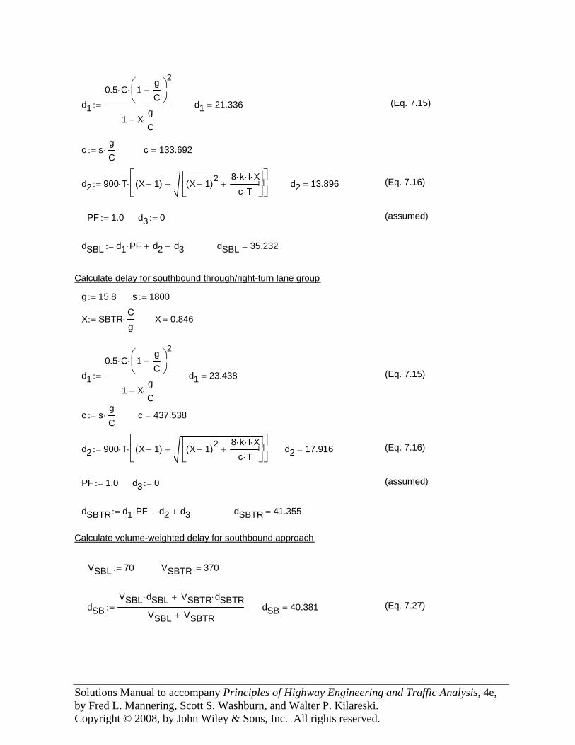
Solutions Manual to accompany Principles of Highway Engineering and Traffic Analysis, 4e, by Fred L. Mannering, Scott S. Washburn, and Walter P. Kilareski. Copyright © 2008, by John Wiley & Sons, Inc. All rights reserved.
d1 23.438= (Eq. 7.15)
c sgC⋅:= c 437.538=
d2 900 T⋅ X 1−( ) X 1−( )28 k⋅ I⋅ X⋅
c T⋅+
⎡⎢⎣
⎤⎥⎦
+⎡⎢⎣
⎤⎥⎦
⋅:= d2 17.916= (Eq. 7.16)
PF 1.0:= d3 0:= (assumed)
dSBTR d1 PF⋅ d2+ d3+:= dSBTR 41.355=
Calculate volume-weighted delay for southbound approach
VSBL 70:= VSBTR 370:=
dSBVSBL dSBL⋅ VSBTR dSBTR⋅+
VSBL VSBTR+:= dSB 40.381= (Eq. 7.27)
d1
0.5 C⋅ 1gC
−⎛⎜⎝
⎞⎟⎠
2⋅
1 XgC⋅−
:= d1 21.336= (Eq. 7.15)
c sgC⋅:= c 133.692=
d2 900 T⋅ X 1−( ) X 1−( )28 k⋅ I⋅ X⋅
c T⋅+
⎡⎢⎣
⎤⎥⎦
+⎡⎢⎣
⎤⎥⎦
⋅:= d2 13.896= (Eq. 7.16)
PF 1.0:= d3 0:= (assumed)
dSBL d1 PF⋅ d2+ d3+:= dSBL 35.232=
Calculate delay for southbound through/right-turn lane group
g 15.8:= s 1800:=
X SBTRCg⋅:= X 0.846=
d1
0.5 C⋅ 1gC
−⎛⎜⎝
⎞⎟⎠
2⋅
1 XgC⋅−
:=

Solutions Manual to accompany Principles of Highway Engineering and Traffic Analysis, 4e, by Fred L. Mannering, Scott S. Washburn, and Walter P. Kilareski. Copyright © 2008, by John Wiley & Sons, Inc. All rights reserved.
Calculate volume-weighted delay for entire intersection
dVEBL VEBTR+( ) dEB⋅ VWBL VWBTR+( ) dWB⋅+ VNBL VNBTR+( ) dNB⋅+ VSBL VSBTR+( ) dSB⋅+
VEBL VEBTR+( ) VWBL VWBTR+( )+ VNBL VNBTR+( )+ VSBL VSBTR+( )+:=
d 34= (Eq. 7.28)
LOS of the intersection is C (Table 7.4)
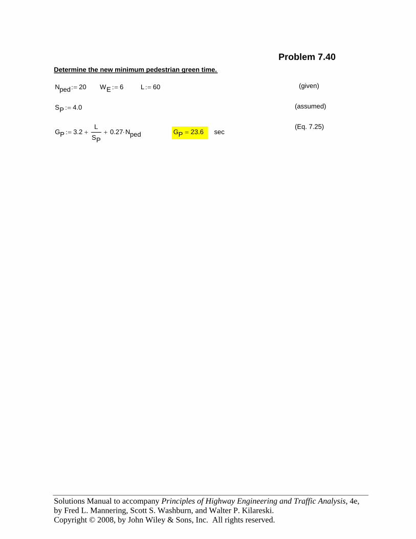
Solutions Manual to accompany Principles of Highway Engineering and Traffic Analysis, 4e, by Fred L. Mannering, Scott S. Washburn, and Walter P. Kilareski. Copyright © 2008, by John Wiley & Sons, Inc. All rights reserved.
Problem 7.40Determine the new minimum pedestrian green time.
Nped 20:= WE 6:= L 60:= (given)
SP 4.0:= (assumed)
(Eq. 7.25)GP 3.2
LSP
+ 0.27 Nped⋅+:= GP 23.6= sec
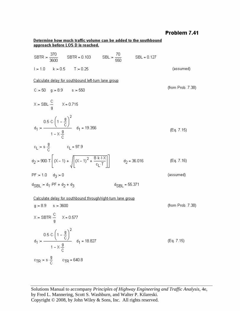
Solutions Manual to accompany Principles of Highway Engineering and Traffic Analysis, 4e, by Fred L. Mannering, Scott S. Washburn, and Walter P. Kilareski. Copyright © 2008, by John Wiley & Sons, Inc. All rights reserved.
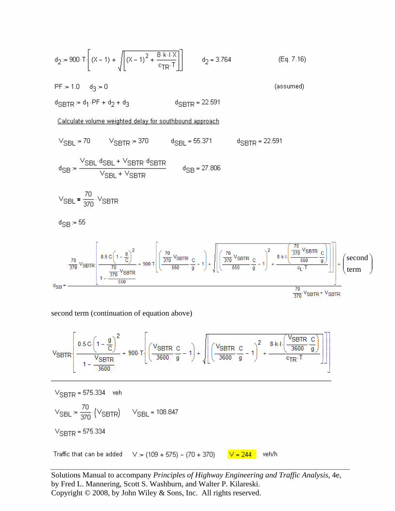
Solutions Manual to accompany Principles of Highway Engineering and Traffic Analysis, 4e, by Fred L. Mannering, Scott S. Washburn, and Walter P. Kilareski. Copyright © 2008, by John Wiley & Sons, Inc. All rights reserved.
second term (continuation of equation above)
⎟⎟⎠
⎞⎜⎜⎝
⎛termsecond
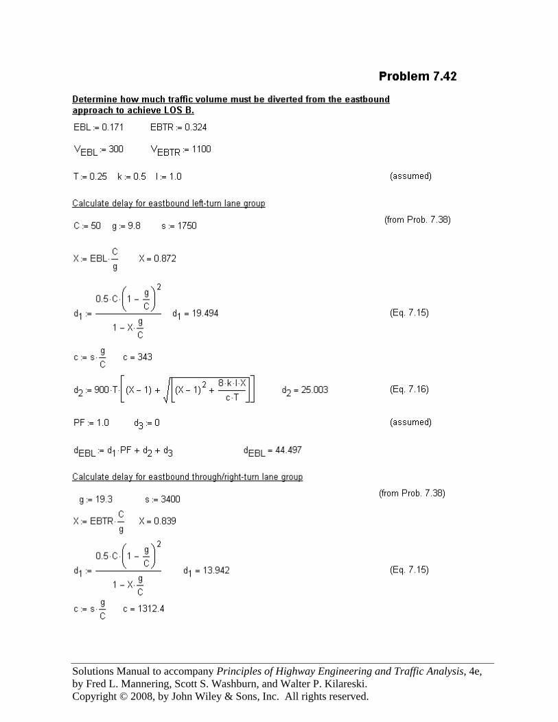
Solutions Manual to accompany Principles of Highway Engineering and Traffic Analysis, 4e, by Fred L. Mannering, Scott S. Washburn, and Walter P. Kilareski. Copyright © 2008, by John Wiley & Sons, Inc. All rights reserved.
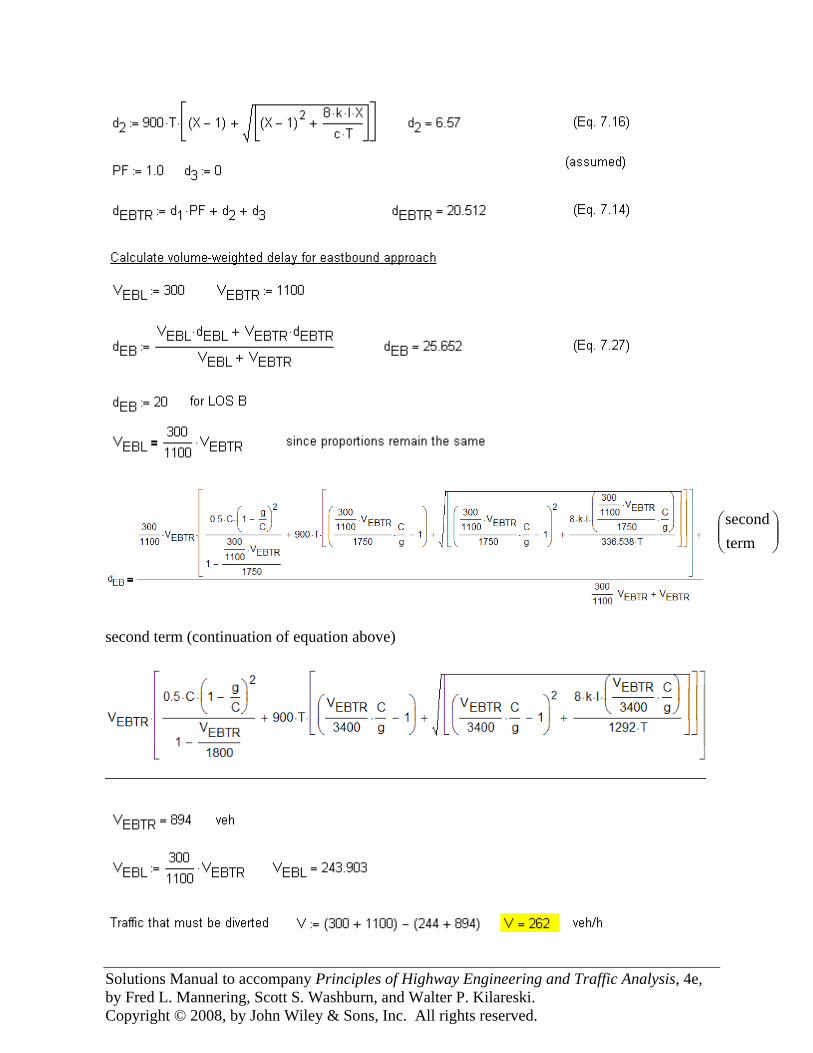
Solutions Manual to accompany Principles of Highway Engineering and Traffic Analysis, 4e, by Fred L. Mannering, Scott S. Washburn, and Walter P. Kilareski. Copyright © 2008, by John Wiley & Sons, Inc. All rights reserved.
second term (continuation of equation above)
⎟⎟⎠
⎞⎜⎜⎝
⎛termsecond
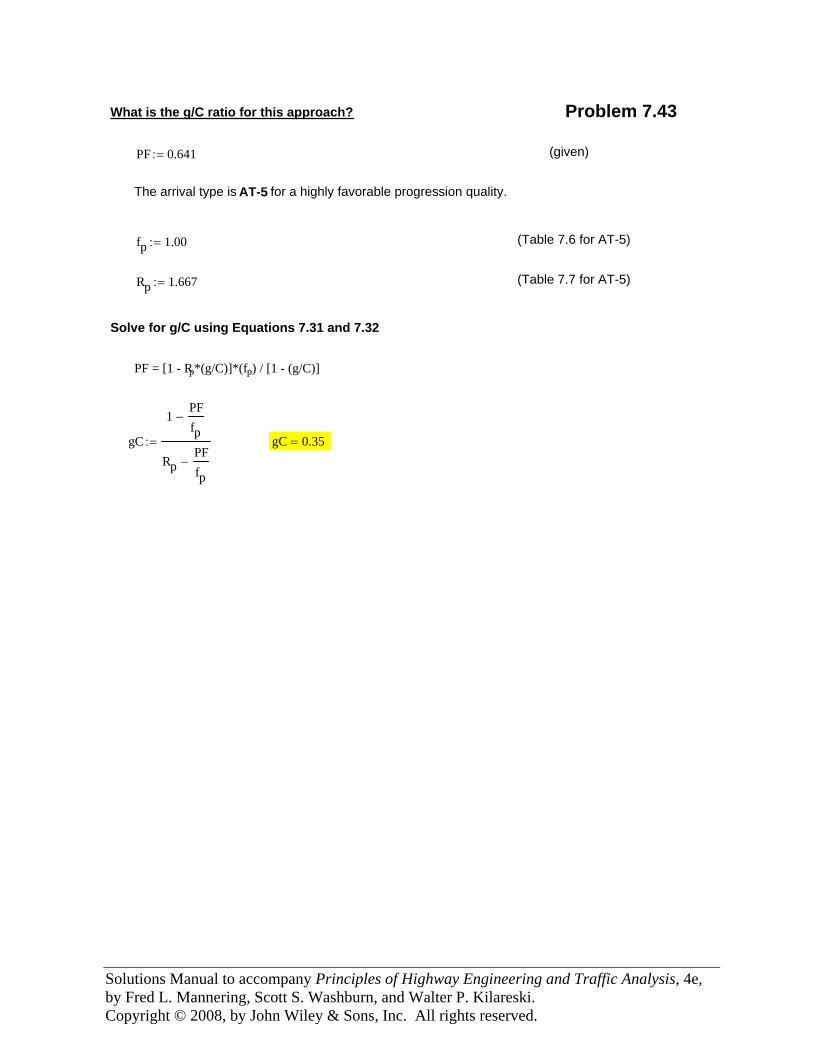
Solutions Manual to accompany Principles of Highway Engineering and Traffic Analysis, 4e, by Fred L. Mannering, Scott S. Washburn, and Walter P. Kilareski. Copyright © 2008, by John Wiley & Sons, Inc. All rights reserved.
What is the g/C ratio for this approach? Problem 7.43
PF 0.641:= (given)
The arrival type is AT-5 for a highly favorable progression quality.
fp 1.00:= (Table 7.6 for AT-5)
Rp 1.667:= (Table 7.7 for AT-5)
Solve for g/C using Equations 7.31 and 7.32
PF = [1 - Rp*(g/C)]*(fp) / [1 - (g/C)]
gC
1PFfp
−
RpPFfp
−
:= gC 0.35=
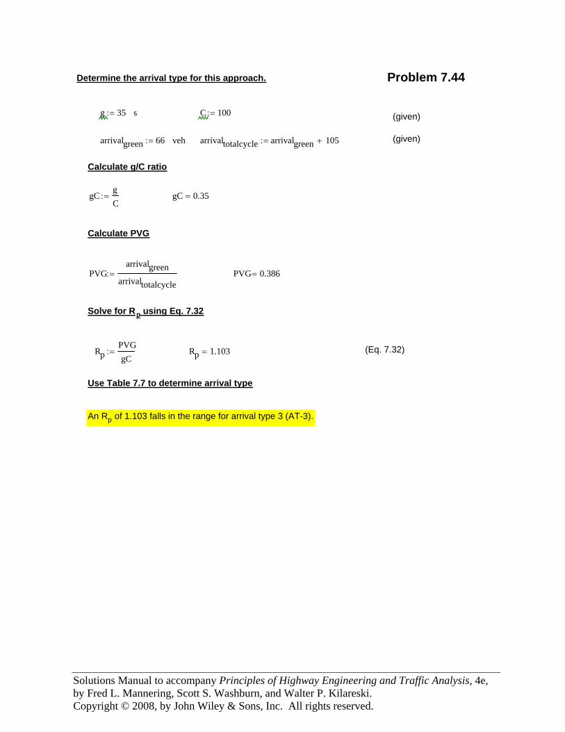
Solutions Manual to accompany Principles of Highway Engineering and Traffic Analysis, 4e, by Fred L. Mannering, Scott S. Washburn, and Walter P. Kilareski. Copyright © 2008, by John Wiley & Sons, Inc. All rights reserved.
Determine the arrival type for this approach. Problem 7.44
g 35:= s C 100:= (given)
arrivalgreen 66:= veh arrivaltotalcycle arrivalgreen 105+:= (given)
Calculate g/C ratio
gCgC
:= gC 0.35=
Calculate PVG
PVGarrivalgreen
arrivaltotalcycle:= PVG 0.386=
Solve for Rp using Eq. 7.32
RpPVGgC
:= Rp 1.103= (Eq. 7.32)
Use Table 7.7 to determine arrival type
An Rp of 1.103 falls in the range for arrival type 3 (AT-3).
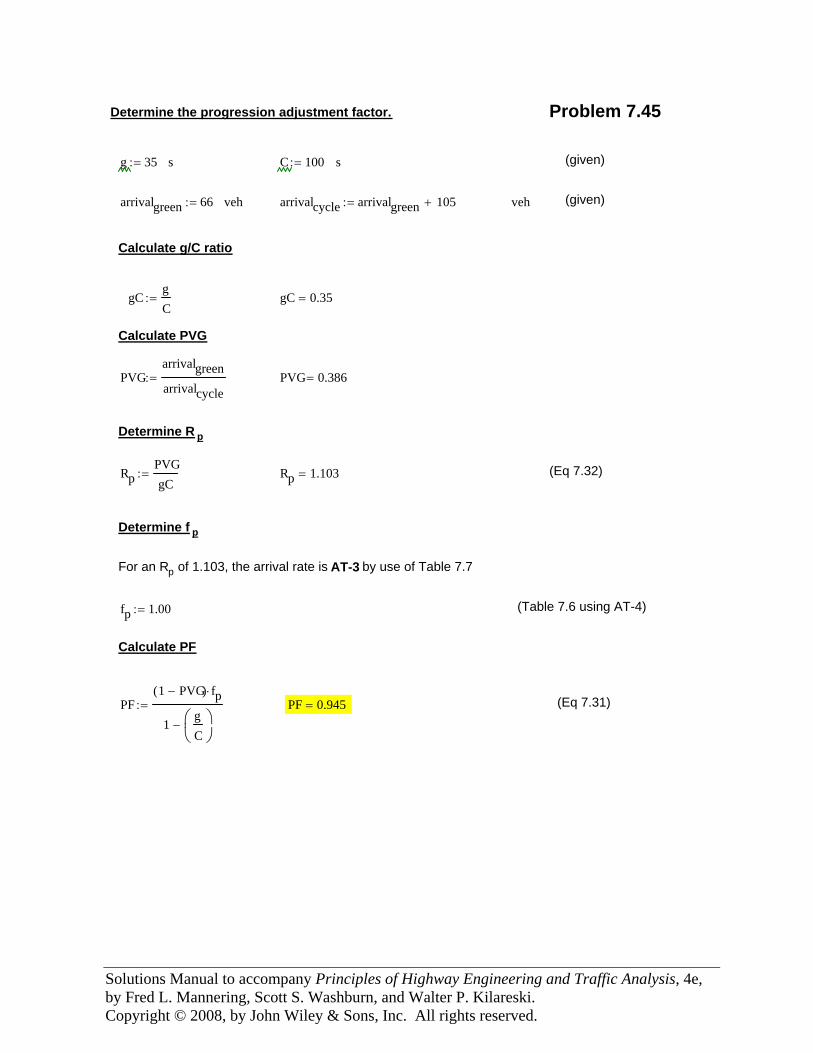
Solutions Manual to accompany Principles of Highway Engineering and Traffic Analysis, 4e, by Fred L. Mannering, Scott S. Washburn, and Walter P. Kilareski. Copyright © 2008, by John Wiley & Sons, Inc. All rights reserved.
Determine the progression adjustment factor. Problem 7.45
g 35:= s C 100:= s (given)
arrivalgreen 66:= veh arrivalcycle arrivalgreen 105+:= veh (given)
Calculate g/C ratio
gCgC
:= gC 0.35=
Calculate PVG
PVGarrivalgreenarrivalcycle
:= PVG 0.386=
Determine R p
RpPVGgC
:= Rp 1.103= (Eq 7.32)
Determine f p
For an Rp of 1.103, the arrival rate is AT-3 by use of Table 7.7
fp 1.00:= (Table 7.6 using AT-4)
Calculate PF
PF1 PVG−( ) fp⋅
1gC
⎛⎜⎝
⎞⎟⎠
−
:= PF 0.945= (Eq 7.31)
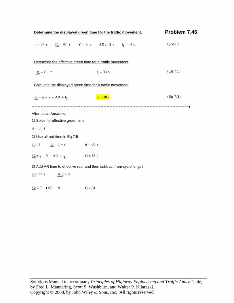
Solutions Manual to accompany Principles of Highway Engineering and Traffic Analysis, 4e, by Fred L. Mannering, Scott S. Washburn, and Walter P. Kilareski. Copyright © 2008, by John Wiley & Sons, Inc. All rights reserved.
Determine the displayed green time for the traffic movement. Problem 7.46
r 37:= s C 70:= s Y 5:= s AR 2:= s tL 4:= s (given)
Determine the effective green time for a traffic movement
g C r−:= g 33= s (Eq 7.5)
Calculate the displayed green time for a traffic movement
G g Y− AR− tL+:= G 30= s (Eq 7.3)
−−−−−−−−−−−−−−−−−−−−−−−−−−−−−−−−−−−−−−−−−−−−−−−−−−−−−−− −−−−−−−−−−−−−−−−−−−−−−−−−−−−−−−−−−−−−−−−Alternative Answers:
1) Solve for effective green time
g 33= s
2) Use all-red time in Eq 7.5
r 2:= g C r−:= g 68= s
G g Y− AR− tL+:= G 65= s
3) Add AR time to effective red, and then subtract from cycle length
r 37:= s AR 2:=
G C AR r+( )−:= G 31=
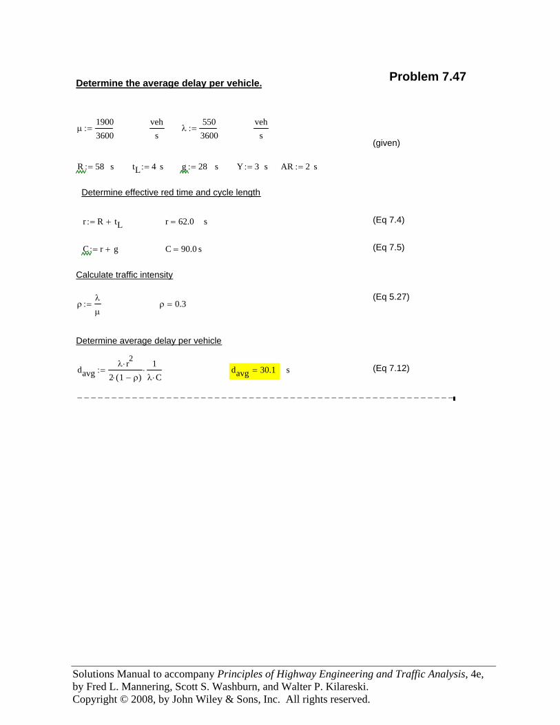
Solutions Manual to accompany Principles of Highway Engineering and Traffic Analysis, 4e, by Fred L. Mannering, Scott S. Washburn, and Walter P. Kilareski. Copyright © 2008, by John Wiley & Sons, Inc. All rights reserved.
Problem 7.47Determine the average delay per vehicle.
μ19003600
:=veh
sλ
5503600
:=veh
s(given)
R 58:= s tL 4:= s g 28:= s Y 3:= s AR 2:= s
Determine effective red time and cycle length
r R tL+:= r 62.0= s (Eq 7.4)
C r g+:= C 90.0= s (Eq 7.5)
Calculate traffic intensity
(Eq 5.27)ρ
λ
μ:= ρ 0.3=
Determine average delay per vehicle
davgλ r2⋅
2 1 ρ−( )⋅
1λ C⋅⋅:= davg 30.1= s (Eq 7.12)
−−−−−−−−−−−−−−−−−−−−−−−−−−−−−−−−−−−−−−−−−−−−−−−−−−−−−−−
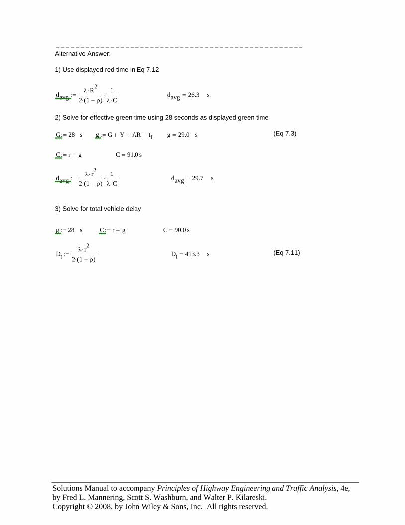
Solutions Manual to accompany Principles of Highway Engineering and Traffic Analysis, 4e, by Fred L. Mannering, Scott S. Washburn, and Walter P. Kilareski. Copyright © 2008, by John Wiley & Sons, Inc. All rights reserved.
−−−−−−−−−−−−−−−−−−−−−−−−−−−−−−−−−−−−−−−−−−−−−−−−−−Alternative Answer:
1) Use displayed red time in Eq 7.12
davgλ R2⋅
2 1 ρ−( )⋅
1λ C⋅⋅:= davg 26.3= s
2) Solve for effective green time using 28 seconds as displayed green time
G 28:= s g G Y+ AR+ tL−:= g 29.0= s (Eq 7.3)
C r g+:= C 91.0= s
davgλ r2⋅
2 1 ρ−( )⋅
1λ C⋅⋅:= davg 29.7= s
3) Solve for total vehicle delay
g 28:= s C r g+:= C 90.0= s
Dtλ r2⋅
2 1 ρ−( )⋅:= Dt 413.3= s (Eq 7.11)
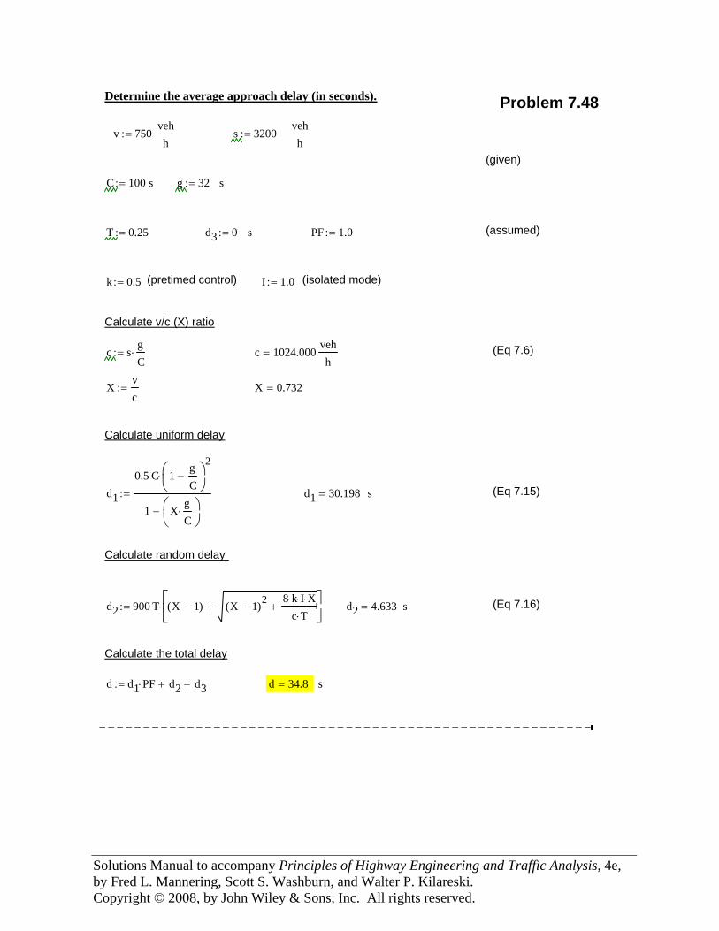
Solutions Manual to accompany Principles of Highway Engineering and Traffic Analysis, 4e, by Fred L. Mannering, Scott S. Washburn, and Walter P. Kilareski. Copyright © 2008, by John Wiley & Sons, Inc. All rights reserved.
Determine the average approach delay (in seconds). Problem 7.48
v 750:=vehh
s 3200:=vehh
(given)
C 100:= s g 32:= s
T 0.25:= d3 0:= s PF 1.0:= (assumed)
k 0.5:= (pretimed control) I 1.0:= (isolated mode)
Calculate v/c (X) ratio
c sgC⋅:= c 1024.000=
vehh
(Eq 7.6)
Xvc
:= X 0.732=
Calculate uniform delay
d1
0.5 C⋅ 1gC
−⎛⎜⎝
⎞⎟⎠
2⋅
1 XgC⋅⎛⎜
⎝⎞⎟⎠
−
:= d1 30.198= s (Eq 7.15)
Calculate random delay
d2 900 T⋅ X 1−( ) X 1−( )2 8 k⋅ I⋅ X⋅c T⋅
++⎡⎢⎣
⎤⎥⎦
⋅:= d2 4.633= s (Eq 7.16)
Calculate the total delay
d d1 PF⋅ d2+ d3+:= d 34.8= s
−−−−−−−−−−−−−−−−−−−−−−−−−−−−−−−−−−−−−−−−−−−−−−−−−−−−−−−−
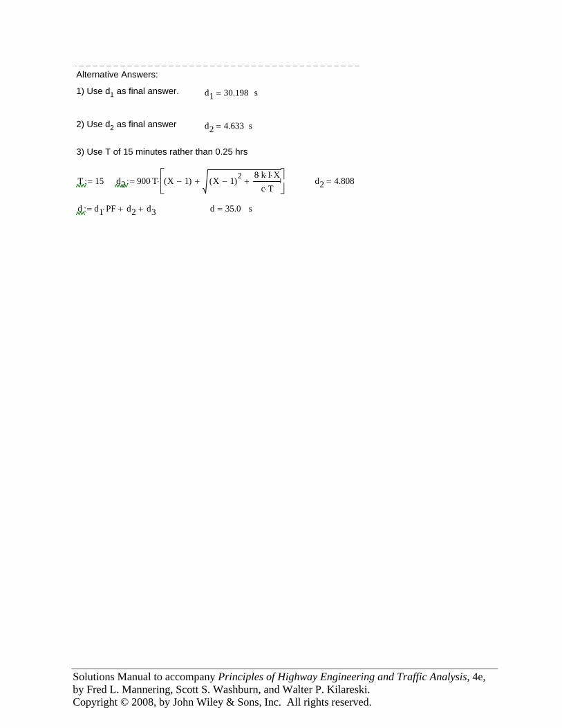
Solutions Manual to accompany Principles of Highway Engineering and Traffic Analysis, 4e, by Fred L. Mannering, Scott S. Washburn, and Walter P. Kilareski. Copyright © 2008, by John Wiley & Sons, Inc. All rights reserved.
−−−−−−−−−−−−−−−−−−−−−−−−−−−−−−−−−−−−−−−−−−Alternative Answers:
1) Use d1 as final answer. d1 30.198= s
2) Use d2 as final answer d2 4.633= s
3) Use T of 15 minutes rather than 0.25 hrs
T 15:= d2 900 T⋅ X 1−( ) X 1−( )2 8 k⋅ I⋅ X⋅c T⋅
++⎡⎢⎣
⎤⎥⎦
⋅:= d2 4.808=
d d1 PF⋅ d2+ d3+:= d 35.0= s
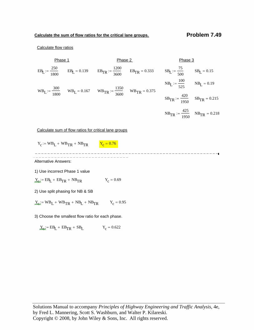
Solutions Manual to accompany Principles of Highway Engineering and Traffic Analysis, 4e, by Fred L. Mannering, Scott S. Washburn, and Walter P. Kilareski. Copyright © 2008, by John Wiley & Sons, Inc. All rights reserved.
Calculate the sum of flow ratios for the critical lane groups.
Problem 7.49
Calculate flow ratios
Phase 1 Phase 2 Phase 3
EBL2501800
:= EBL 0.139= EBTR12003600
:= EBTR 0.333= SBL75500
:= SBL 0.15=
NBL100525
:= NBL 0.19=
WBL3001800
:= WBL 0.167= WBTR13503600
:= WBTR 0.375=
SBTR4201950
:= SBTR 0.215=
NBTR4251950
:= NBTR 0.218=
Calculate sum of flow ratios for critical lane groups
Yc WBL WBTR+ NBTR+:= Yc 0.76=
−−−−−−−−−−−−−−−−−−−−−−−−−−−−−−−−−−−−−−−−−−−−−−−−−−−−−−−−−−− −−−−−−−−−−−−−−−−−−−−−−−−−−−−−−−Alternative Answers:
1) Use incorrect Phase 1 value
Yc EBL EBTR+ NBTR+:= Yc 0.69=
2) Use split phasing for NB & SB
Yc WBL WBTR+ NBL+ NBTR+:= Yc 0.95=
3) Choose the smallest flow ratio for each phase.
Yc EBL EBTR+ SBL+:= Yc 0.622=
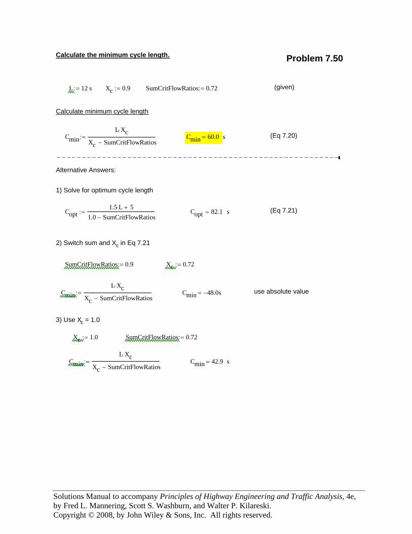
Solutions Manual to accompany Principles of Highway Engineering and Traffic Analysis, 4e, by Fred L. Mannering, Scott S. Washburn, and Walter P. Kilareski. Copyright © 2008, by John Wiley & Sons, Inc. All rights reserved.
Calculate the minimum cycle length. Problem 7.50
L 12:= s Xc 0.9:= SumCritFlowRatios 0.72:= (given)
Calculate minimum cycle length
CminL Xc⋅
Xc SumCritFlowRatios−:= Cmin 60.0= s (Eq 7.20)
−−−−−−−−−−−−−−−−−−−−−−−−−−−−−−−−−−−−−−−−−−−−−−−−−−−−−−−− Alternative Answers:
1) Solve for optimum cycle length
Copt1.5 L⋅ 5+
1.0 SumCritFlowRatios−:= Copt 82.1= s (Eq 7.21)
2) Switch sum and Xc in Eq 7.21
SumCritFlowRatios 0.9:= Xc 0.72:=
CminL Xc⋅
Xc SumCritFlowRatios−:= Cmin 48.0−= s use absolute value
3) Use Xc = 1.0
Xc 1.0:= SumCritFlowRatios 0.72:=
CminL Xc⋅
Xc SumCritFlowRatios−:= Cmin 42.9= s
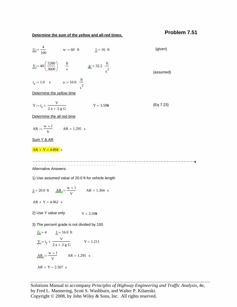
Solutions Manual to accompany Principles of Highway Engineering and Traffic Analysis, 4e, by Fred L. Mannering, Scott S. Washburn, and Walter P. Kilareski. Copyright © 2008, by John Wiley & Sons, Inc. All rights reserved.
Problem 7.51Determine the sum of the yellow and all-red times.
G4
100:= w 60:= ft l 16:= ft (given)
V 4052803600
⎛⎜⎝
⎞⎟⎠
⋅:=fts
g 32.2:=ft
s2(assumed)
tr 1.0:= s a 10.0:=ft
s2
Determine the yellow time
Y trV
2 a⋅ 2 g⋅ G⋅++:= Y 3.599= s (Eq 7.23)
Determine the all red time
ARw l+
V:= AR 1.295= s
Sum Y & AR
AR Y+ 4.894= s
−−−−−−−−−−−−−−−−−−−−−−−−−−−−−−−−−−−−−−−−−−−−−−−−−−−−−−−− −−−−−−−−−−−−−−−−−−−−−−−−−−−−−Alternative Answers:
1) Use assumed value of 20.0 ft for vehicle length
l 20.0:= ft ARw l+
V:= AR 1.364= s
AR Y+ 4.962= s
2) Use Y value only Y 3.599= s
3) The percent grade is not divided by 100
G 4:= l 16.0:= ft
Y trV
2 a⋅ 2 g⋅ G⋅++:= Y 1.211=
ARw l+
V:= AR 1.295= s
AR Y+ 2.507= s
Solutions Manual to accompany
Principles of Highway Engineering and Traffic Analysis, 4e
By Fred L. Mannering, Scott S. Washburn, and Walter P. Kilareski
Chapter 8 Travel Demand and Traffic Forecasting
U.S. Customary Units
Copyright © 2008, by John Wiley & Sons, Inc. All rights reserved.
Solutions Manual to accompany Principles of Highway Engineering and Traffic Analysis, 4e, by Fred L. Mannering, Scott S. Washburn, and Walter P. Kilareski. Copyright © 2008, by John Wiley & Sons, Inc. All rights reserved.
Preface The solutions to the fourth edition of Principles of Highway Engineering and Traffic Analysis were prepared with the Mathcad1 software program. You will notice several notation conventions that you may not be familiar with if you are not a Mathcad user. Most of these notation conventions are self-explanatory or easily understood. The most common Mathcad specific notations in these solutions relate to the equals sign. You will notice the equals sign being used in three different contexts, and Mathcad uses three different notations to distinguish between each of these contexts. The differences between these equals sign notations are explained as follows.
• The ‘:=’ (colon-equals) is an assignment operator, that is, the value of the variable or expression on the left side of ‘:=’is set equal to the value of the expression on the right side. For example, in the statement, L := 1234, the variable ‘L’ is assigned (i.e., set equal to) the value of 1234. Another example is x := y + z. In this case, x is assigned the value of y + z.
• The ‘==’ (bold equals) is used when the Mathcad function solver was used to find the value of a variable in the equation. For example, in the equation
, the == is used to tell Mathcad that the value of the expression on the left side needs to equal the value of the expression on the right side. Thus, the Mathcad solver can be employed to find a value for the variable ‘t’ that satisfies this relationship. This particular example is from a problem where the function for arrivals at some time ‘t’ is set equal to the function for departures at some time ‘t’ to find the time to queue clearance.
• The ‘=’ (standard equals) is used for a simple numeric evaluation. For example, referring to the x := y + z assignment used previously, if the value of y was 10 [either by assignment (with :=), or the result of an equation solution (through the use of ==) and the value of z was 15, then the expression ‘x =’ would yield 25. Another example would be as follows: s := 1800/3600, with s = 0.5. That is, ‘s’ was assigned the value of 1800 divided by 3600 (using :=), which equals 0.5 (as given by using =).
Another symbol you will see frequently is ‘→’. In these solutions, it is used to perform an evaluation of an assignment expression in a single statement. For example, in the following
statement, , Q(t) is assigned the value of Arrivals(t) – Departures(t), and this evaluates to 2.2t – 0.10t2. Finally, to assist in quickly identifying the final answer, or answers, for what is being asked in the problem statement, yellow highlighting has been used (which will print as light gray). 1 www.mathcad.com
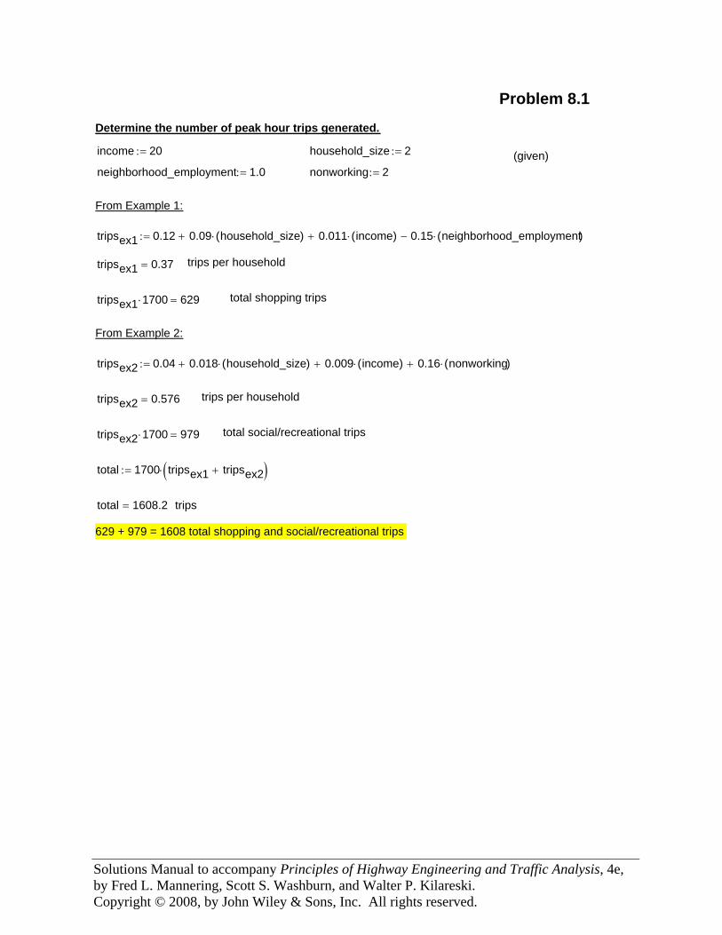
Solutions Manual to accompany Principles of Highway Engineering and Traffic Analysis, 4e, by Fred L. Mannering, Scott S. Washburn, and Walter P. Kilareski. Copyright © 2008, by John Wiley & Sons, Inc. All rights reserved.
629 + 979 = 1608 total shopping and social/recreational trips
tripstotal 1608.2=
total 1700 tripsex1 tripsex2+( )⋅:=
total social/recreational tripstripsex2 1700⋅ 979=
trips per householdtripsex2 0.576=
tripsex2 0.04 0.018 household_size( )⋅+ 0.009 income( )⋅+ 0.16 nonworking( )⋅+:=
From Example 2:
total shopping tripstripsex1 1700⋅ 629=
trips per householdtripsex1 0.37=
tripsex1 0.12 0.09 household_size( )⋅+ 0.011 income( )⋅+ 0.15 neighborhood_employment( )⋅−:=
From Example 1:
nonworking 2:=neighborhood_employment 1.0:=(given)household_size 2:=income 20:=
Determine the number of peak hour trips generated.
Problem 8.1
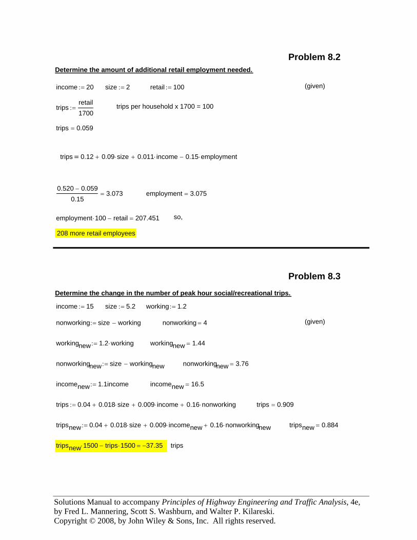
Solutions Manual to accompany Principles of Highway Engineering and Traffic Analysis, 4e, by Fred L. Mannering, Scott S. Washburn, and Walter P. Kilareski. Copyright © 2008, by John Wiley & Sons, Inc. All rights reserved.
208 more retail employees
so,employment 100⋅ retail− 207.451=
employment 3.075=0.520 0.059−
0.153.073=
trips 0.12 0.09 size⋅+ 0.011 income⋅+ 0.15 employment⋅−
trips 0.059=
trips per household x 1700 = 100tripsretail1700
:=
(given)retail 100:=size 2:=income 20:=
Determine the amount of additional retail employment needed.
Problem 8.2
tripstripsnew 1500⋅ trips 1500⋅− 37.35−=
tripsnew 0.884=tripsnew 0.04 0.018 size⋅+ 0.009 incomenew⋅+ 0.16 nonworkingnew⋅+:=
trips 0.909=trips 0.04 0.018 size⋅+ 0.009 income⋅+ 0.16 nonworking⋅+:=
incomenew 16.5=incomenew 1.1income:=
nonworkingnew 3.76=nonworkingnew size workingnew−:=
workingnew 1.44=workingnew 1.2 working⋅:=
(given)nonworking 4=nonworking size working−:=
working 1.2:=size 5.2:=income 15:=
Determine the change in the number of peak hour social/recreational trips.
Problem 8.3
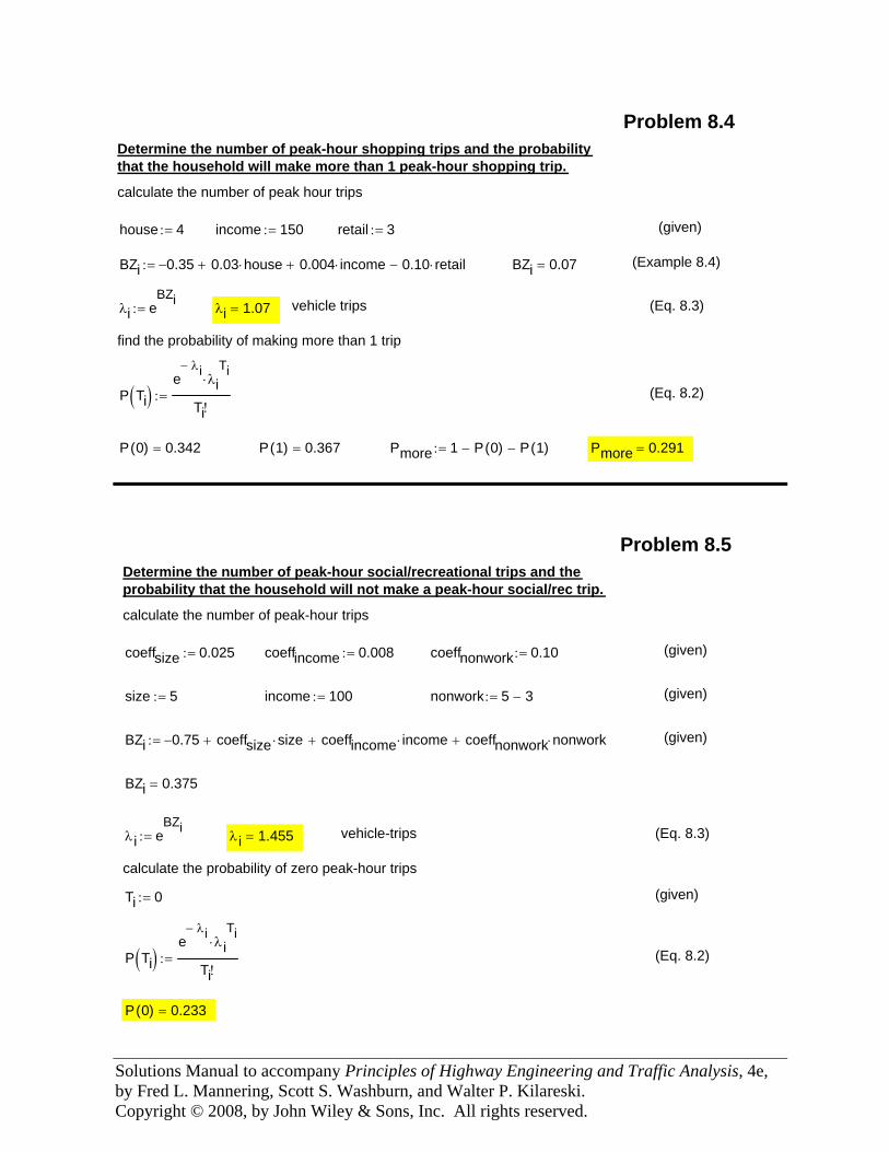
Solutions Manual to accompany Principles of Highway Engineering and Traffic Analysis, 4e, by Fred L. Mannering, Scott S. Washburn, and Walter P. Kilareski. Copyright © 2008, by John Wiley & Sons, Inc. All rights reserved.
Pmore 0.291=Pmore 1 P 0( )− P 1( )−:=P 1( ) 0.367=P 0( ) 0.342=
(Eq. 8.2)P Ti( )e
λi−λi
Ti⋅
Ti!:=
find the probability of making more than 1 trip
(Eq. 8.3)vehicle tripsλi 1.07=λi eBZi
:=
(Example 8.4)BZi 0.07=BZi 0.35− 0.03 house⋅+ 0.004 income⋅+ 0.10 retail⋅−:=
(given)retail 3:=income 150:=house 4:=
calculate the number of peak hour trips
Determine the number of peak-hour shopping trips and the probabilitythat the household will make more than 1 peak-hour shopping trip.
Problem 8.4
Problem 8.5Determine the number of peak-hour social/recreational trips and theprobability that the household will not make a peak-hour social/rec trip.
calculate the number of peak-hour trips
coeffsize 0.025:= coeffincome 0.008:= coeffnonwork 0.10:= (given)
size 5:= income 100:= nonwork 5 3−:= (given)
BZi 0.75− coeffsize size⋅+ coeffincome income⋅+ coeffnonwork nonwork⋅+:= (given)
BZi 0.375=
λi eBZi
:= λi 1.455= vehicle-trips (Eq. 8.3)
calculate the probability of zero peak-hour trips
Ti 0:= (given)
P Ti( )e
λi−λi
Ti⋅
Ti!:= (Eq. 8.2)
P 0( ) 0.233=
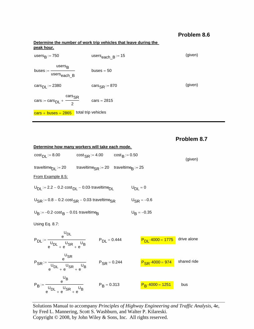
Solutions Manual to accompany Principles of Highway Engineering and Traffic Analysis, 4e, by Fred L. Mannering, Scott S. Washburn, and Walter P. Kilareski. Copyright © 2008, by John Wiley & Sons, Inc. All rights reserved.
Problem 8.6Determine the number of work trip vehicles that leave during the peak hour.
usersB 750:= userseach_B 15:= (given)
busesusersB
userseach_B:= buses 50=
carsDL 2380:= carsSR 870:= (given)
cars carsDLcarsSR
2+:= cars 2815=
cars buses+ 2865= total trip vehicles
busPB 4000⋅ 1251=PB 0.313=PBe
UB
eUDL e
USR+ e
UB+
:=
shared ridePSR 4000⋅ 974=PSR 0.244=PSRe
USR
eUDL e
USR+ e
UB+
:=
drive alonePDL 4000⋅ 1775=PDL 0.444=PDLe
UDL
eUDL e
USR+ e
UB+
:=
Using Eq. 8.7:
UB 0.35−=UB 0.2− costB⋅ 0.01 traveltimeB⋅−:=
USR 0.6−=USR 0.8 0.2 costSR⋅− 0.03 traveltimeSR⋅−:=
UDL 0=UDL 2.2 0.2 costDL⋅− 0.03 traveltimeDL⋅−:=
From Example 8.5:
traveltimeB 25:=traveltimeSR 20:=traveltimeDL 20:=
(given)costB 0.50:=costSR 4.00:=costDL 8.00:=
Determine how many workers will take each mode.
Problem 8.7
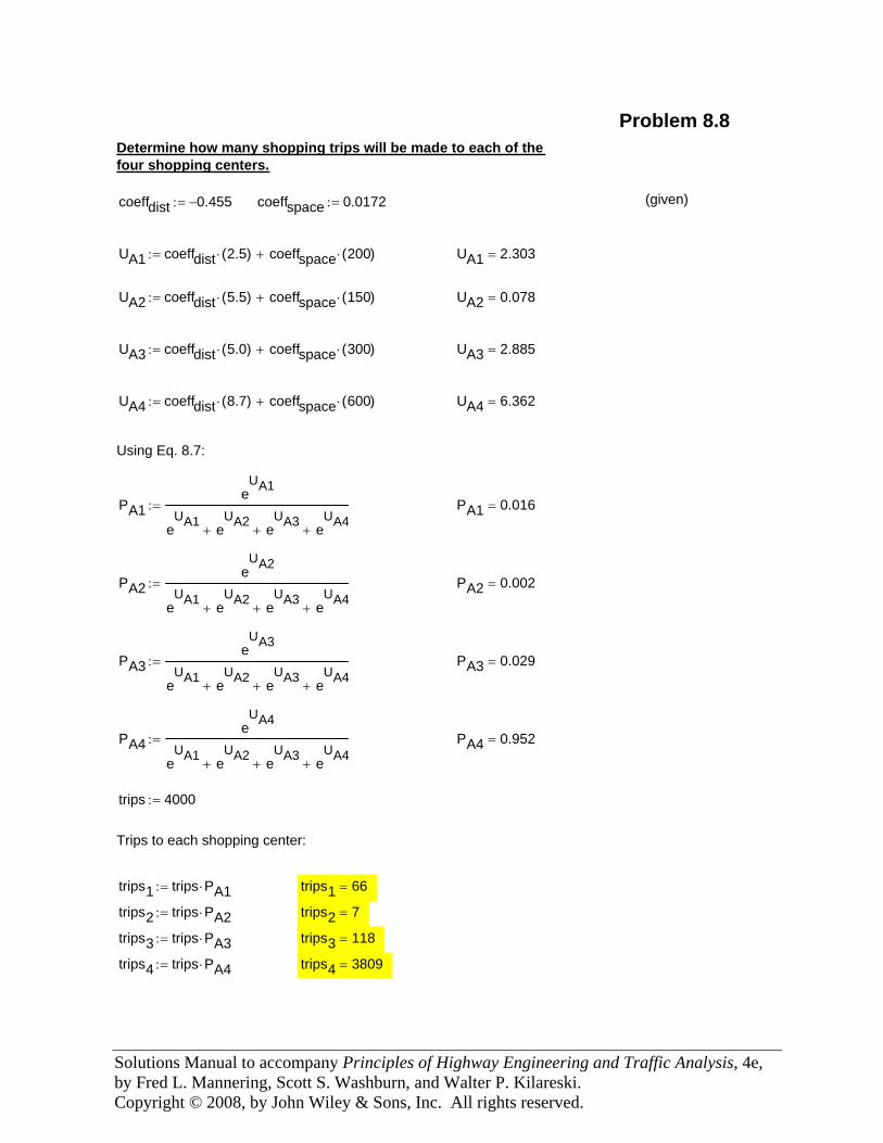
Solutions Manual to accompany Principles of Highway Engineering and Traffic Analysis, 4e, by Fred L. Mannering, Scott S. Washburn, and Walter P. Kilareski. Copyright © 2008, by John Wiley & Sons, Inc. All rights reserved.
trips4 3809=trips4 trips PA4⋅:=
trips3 118=trips3 trips PA3⋅:=
trips2 7=trips2 trips PA2⋅:=
trips1 66=trips1 trips PA1⋅:=
Trips to each shopping center:
trips 4000:=
PA4 0.952=PA4e
UA4
eUA1 e
UA2+ e
UA3+ e
UA4+
:=
PA3 0.029=PA3e
UA3
eUA1 e
UA2+ e
UA3+ e
UA4+
:=
PA2 0.002=PA2e
UA2
eUA1 e
UA2+ e
UA3+ e
UA4+
:=
PA1 0.016=PA1e
UA1
eUA1 e
UA2+ e
UA3+ e
UA4+
:=
Using Eq. 8.7:
UA4 6.362=UA4 coeffdist 8.7( )⋅ coeffspace 600( )⋅+:=
UA3 2.885=UA3 coeffdist 5.0( )⋅ coeffspace 300( )⋅+:=
UA2 0.078=UA2 coeffdist 5.5( )⋅ coeffspace 150( )⋅+:=
UA1 2.303=UA1 coeffdist 2.5( )⋅ coeffspace 200( )⋅+:=
(given)coeffspace 0.0172:=coeffdist 0.455−:=
Determine how many shopping trips will be made to each of thefour shopping centers.
Problem 8.8
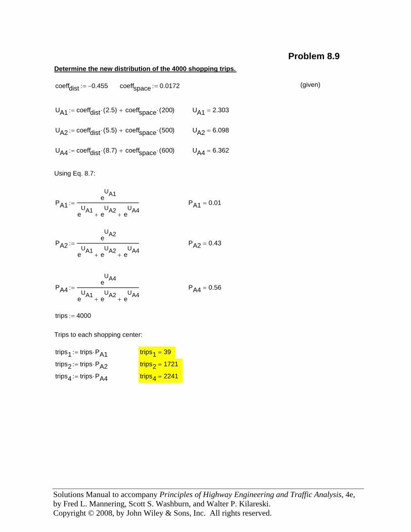
Solutions Manual to accompany Principles of Highway Engineering and Traffic Analysis, 4e, by Fred L. Mannering, Scott S. Washburn, and Walter P. Kilareski. Copyright © 2008, by John Wiley & Sons, Inc. All rights reserved.
trips4 2241=trips4 trips PA4⋅:=
trips2 1721=trips2 trips PA2⋅:=
trips1 39=trips1 trips PA1⋅:=
Trips to each shopping center:
trips 4000:=
PA4 0.56=PA4e
UA4
eUA1 e
UA2+ e
UA4+
:=
PA2 0.43=PA2e
UA2
eUA1 e
UA2+ e
UA4+
:=
PA1 0.01=PA1e
UA1
eUA1 e
UA2+ e
UA4+
:=
Using Eq. 8.7:
UA4 6.362=UA4 coeffdist 8.7( )⋅ coeffspace 600( )⋅+:=
UA2 6.098=UA2 coeffdist 5.5( )⋅ coeffspace 500( )⋅+:=
UA1 2.303=UA1 coeffdist 2.5( )⋅ coeffspace 200( )⋅+:=
(given)coeffspace 0.0172:=coeffdist 0.455−:=
Determine the new distribution of the 4000 shopping trips.
Problem 8.9
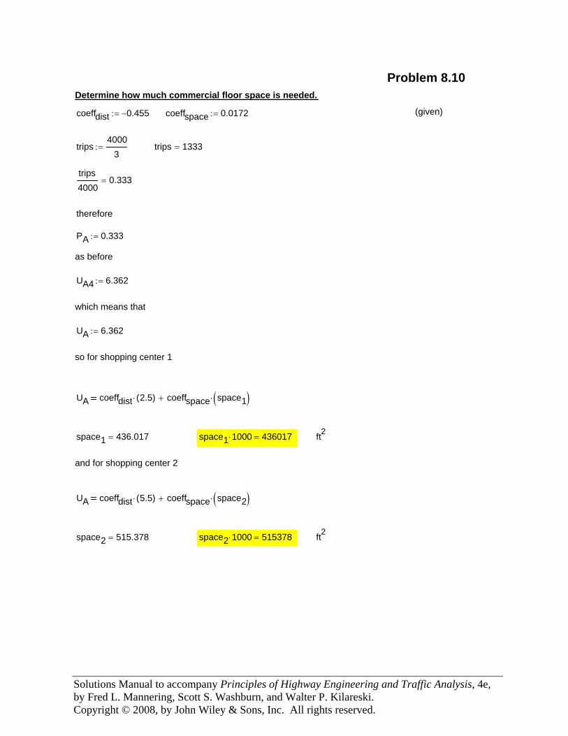
Solutions Manual to accompany Principles of Highway Engineering and Traffic Analysis, 4e, by Fred L. Mannering, Scott S. Washburn, and Walter P. Kilareski. Copyright © 2008, by John Wiley & Sons, Inc. All rights reserved.
ft2space2 1000⋅ 515378=space2 515.378=
UA coeffdist 5.5( )⋅ coeffspace space2( )⋅+
and for shopping center 2
ft2space1 1000⋅ 436017=space1 436.017=
UA coeffdist 2.5( )⋅ coeffspace space1( )⋅+
so for shopping center 1
UA 6.362:=
which means that
UA4 6.362:=
as before
PA 0.333:=
therefore
trips4000
0.333=
trips 1333=trips4000
3:=
(given)coeffspace 0.0172:=coeffdist 0.455−:=
Determine how much commercial floor space is needed.
Problem 8.10
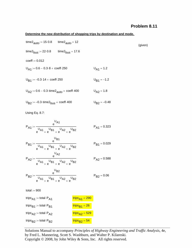
Solutions Manual to accompany Principles of Highway Engineering and Traffic Analysis, 4e, by Fred L. Mannering, Scott S. Washburn, and Walter P. Kilareski. Copyright © 2008, by John Wiley & Sons, Inc. All rights reserved.
PA1e
UA1
eUA1 e
UB1+ e
UA2+ e
UB2+
:= PA1 0.323=
PB1e
UB1
eUA1 e
UB1+ e
UA2+ e
UB2+
:= PB1 0.029=
PA2e
UA2
eUA1 e
UB1+ e
UA2+ e
UB2+
:= PA2 0.588=
PB2e
UB2
eUA1 e
UB1+ e
UA2+ e
UB2+
:= PB2 0.06=
total 900:=
tripsA1 total PA1⋅:= tripsA1 290=
tripsB1 total PB1⋅:= tripsB1 26=
tripsA2 total PA2⋅:= tripsA2 529=
tripsB2 total PB2⋅:= tripsB2 54=
Problem 8.11
Determine the new distribution of shopping trips by destination and mode.
time2auto 15 0.8⋅:= time2auto 12=(given)
time2bus 22 0.8⋅:= time2bus 17.6=
coeff 0.012:=
UA1 0.6 0.3 8⋅− coeff 250⋅+:= UA1 1.2=
UB1 0.3− 14⋅ coeff 250⋅+:= UB1 1.2−=
UA2 0.6 0.3 time2auto⋅− coeff 400⋅+:= UA2 1.8=
UB2 0.3− time2bus⋅ coeff 400⋅+:= UB2 0.48−=
Using Eq. 8.7:
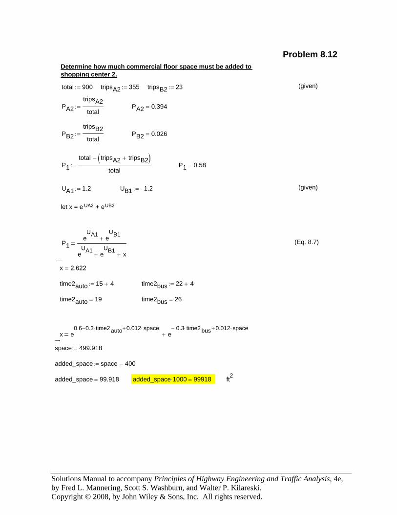
Solutions Manual to accompany Principles of Highway Engineering and Traffic Analysis, 4e, by Fred L. Mannering, Scott S. Washburn, and Walter P. Kilareski. Copyright © 2008, by John Wiley & Sons, Inc. All rights reserved.
Determine how much commercial floor space must be added toshopping center 2.
Problem 8.12
total 900:= tripsA2 355:= tripsB2 23:= (given)
PA2tripsA2
total:= PA2 0.394=
PB2tripsB2
total:= PB2 0.026=
P1total tripsA2 tripsB2+( )−
total:= P1 0.58=
UA1 1.2:= UB1 1.2−:= (given)
let x = e UA2 + eUB2
P1e
UA1 eUB1
+
eUA1 e
UB1+ x+
(Eq. 8.7)
x 2.622=
time2auto 15 4+:= time2bus 22 4+:=
time2auto 19= time2bus 26=
x e0.6 0.3 time2auto⋅− 0.012 space⋅+
e0.3− time2bus⋅ 0.012 space⋅+
+
space 499.918=
added_space space 400−:=
added_space 99.918= added_space 1000⋅ 99918= ft2
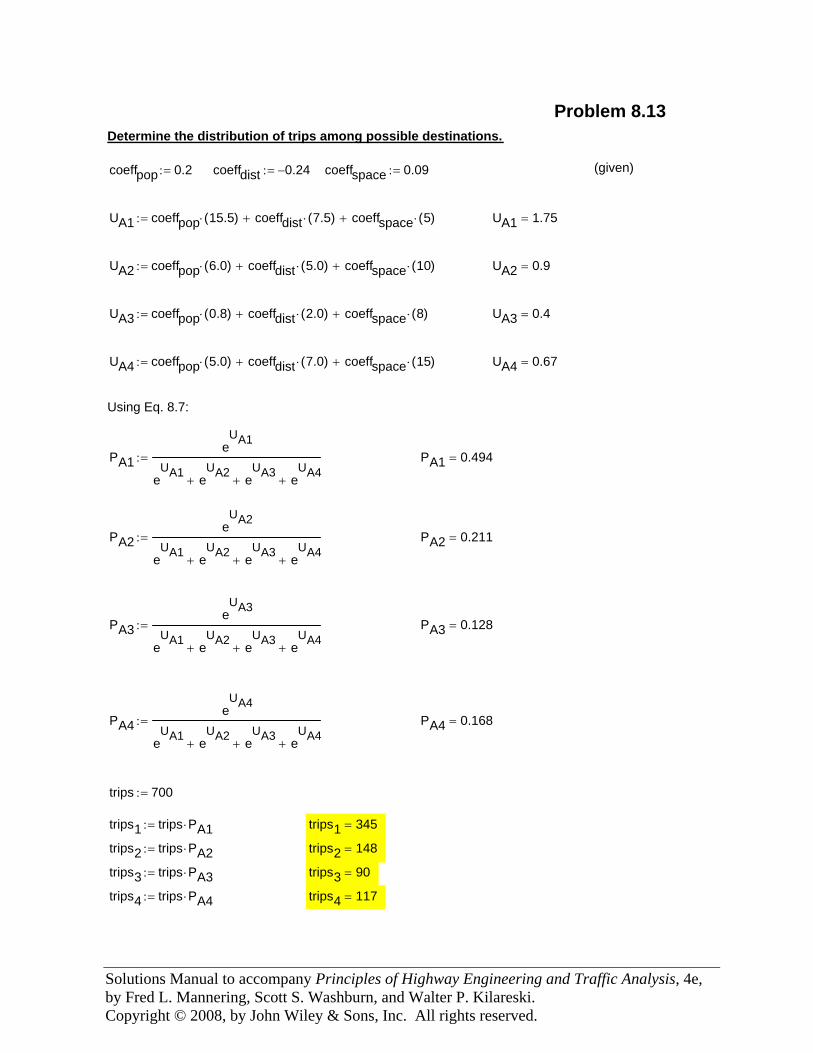
Solutions Manual to accompany Principles of Highway Engineering and Traffic Analysis, 4e, by Fred L. Mannering, Scott S. Washburn, and Walter P. Kilareski. Copyright © 2008, by John Wiley & Sons, Inc. All rights reserved.
trips4 117=trips4 trips PA4⋅:=
trips3 90=trips3 trips PA3⋅:=
trips2 148=trips2 trips PA2⋅:=
trips1 345=trips1 trips PA1⋅:=
trips 700:=
PA4 0.168=PA4e
UA4
eUA1 e
UA2+ e
UA3+ e
UA4+
:=
PA3 0.128=PA3e
UA3
eUA1 e
UA2+ e
UA3+ e
UA4+
:=
PA2 0.211=PA2e
UA2
eUA1 e
UA2+ e
UA3+ e
UA4+
:=
PA1 0.494=PA1e
UA1
eUA1 e
UA2+ e
UA3+ e
UA4+
:=
Using Eq. 8.7:
UA4 0.67=UA4 coeffpop 5.0( )⋅ coeffdist 7.0( )⋅+ coeffspace 15( )⋅+:=
UA3 0.4=UA3 coeffpop 0.8( )⋅ coeffdist 2.0( )⋅+ coeffspace 8( )⋅+:=
UA2 0.9=UA2 coeffpop 6.0( )⋅ coeffdist 5.0( )⋅+ coeffspace 10( )⋅+:=
UA1 1.75=UA1 coeffpop 15.5( )⋅ coeffdist 7.5( )⋅+ coeffspace 5( )⋅+:=
(given)coeffspace 0.09:=coeffdist 0.24−:=coeffpop 0.2:=
Determine the distribution of trips among possible destinations.
Problem 8.13
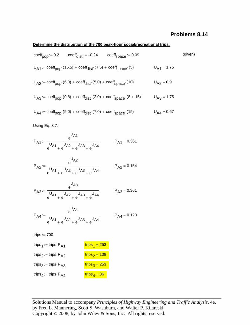
Solutions Manual to accompany Principles of Highway Engineering and Traffic Analysis, 4e, by Fred L. Mannering, Scott S. Washburn, and Walter P. Kilareski. Copyright © 2008, by John Wiley & Sons, Inc. All rights reserved.
trips4 86=trips4 trips PA4⋅:=
trips3 253=trips3 trips PA3⋅:=
trips2 108=trips2 trips PA2⋅:=
trips1 253=trips1 trips PA1⋅:=
trips 700:=
PA4 0.123=PA4e
UA4
eUA1 e
UA2+ e
UA3+ e
UA4+
:=
PA3 0.361=PA3e
UA3
eUA1 e
UA2+ e
UA3+ e
UA4+
:=
PA2 0.154=PA2e
UA2
eUA1 e
UA2+ e
UA3+ e
UA4+
:=
PA1 0.361=PA1e
UA1
eUA1 e
UA2+ e
UA3+ e
UA4+
:=
Using Eq. 8.7:
UA4 0.67=UA4 coeffpop 5.0( )⋅ coeffdist 7.0( )⋅+ coeffspace 15( )⋅+:=
UA3 1.75=UA3 coeffpop 0.8( )⋅ coeffdist 2.0( )⋅+ coeffspace 8 15+( )⋅+:=
UA2 0.9=UA2 coeffpop 6.0( )⋅ coeffdist 5.0( )⋅+ coeffspace 10( )⋅+:=
UA1 1.75=UA1 coeffpop 15.5( )⋅ coeffdist 7.5( )⋅+ coeffspace 5( )⋅+:=
(given)coeffspace 0.09:=coeffdist 0.24−:=coeffpop 0.2:=
Determine the distribution of the 700 peak-hour social/recreational trips.
Problems 8.14

Solutions Manual to accompany Principles of Highway Engineering and Traffic Analysis, 4e, by Fred L. Mannering, Scott S. Washburn, and Walter P. Kilareski. Copyright © 2008, by John Wiley & Sons, Inc. All rights reserved.
ft2added_space 1000⋅ 5523=added_space 5.5=
added_space space 13−:=
space 18.5=
x e 0.9 0.22 14⋅− 0.16 12.4⋅+ .11 space⋅+( ) e 0.22− 17⋅ 0.16 12.4⋅+ .11 space⋅+( )+
x 7.631=
P2and3e
UA2 eUB2
+ eUA3
+ eUB3
+
eUA2 e
UB2+ e
UA3+ e
UB3+ x+
let x = e UA1 + eUB1
(From Ex. 8.8)UB3 2.042−:=UA3 0.178:=UB2 0.564:=UA2 2.124:=
P2and3 0.6=P2and3 1.0 P1−:=
P1 0.40:=
trips1total 200=trips1total 500 0.40⋅:=
Determine how much additional amusement floor space must be added.
Problem 8.15
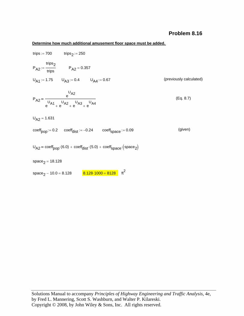
Solutions Manual to accompany Principles of Highway Engineering and Traffic Analysis, 4e, by Fred L. Mannering, Scott S. Washburn, and Walter P. Kilareski. Copyright © 2008, by John Wiley & Sons, Inc. All rights reserved.
ft28.128 1000⋅ 8128=space2 10.0− 8.128=
space2 18.128=
UA2 coeffpop 6.0( )⋅ coeffdist 5.0( )⋅+ coeffspace space2( )⋅+
(given)coeffspace 0.09:=coeffdist 0.24−:=coeffpop 0.2:=
UA2 1.631=
(Eq. 8.7)PA2e
UA2
eUA1 e
UA2+ e
UA3+ e
UA4+
(previously calculated)UA4 0.67:=UA3 0.4:=UA1 1.75:=
PA2 0.357=PA2trips2trips
:=
trips2 250:=trips 700:=
Determine how much additional amusement floor space must be added.
Problem 8.16
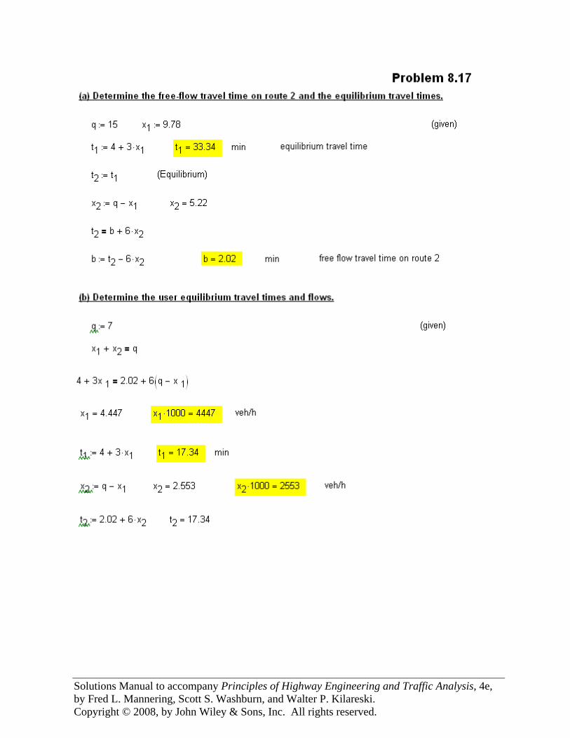
Solutions Manual to accompany Principles of Highway Engineering and Traffic Analysis, 4e, by Fred L. Mannering, Scott S. Washburn, and Walter P. Kilareski. Copyright © 2008, by John Wiley & Sons, Inc. All rights reserved.
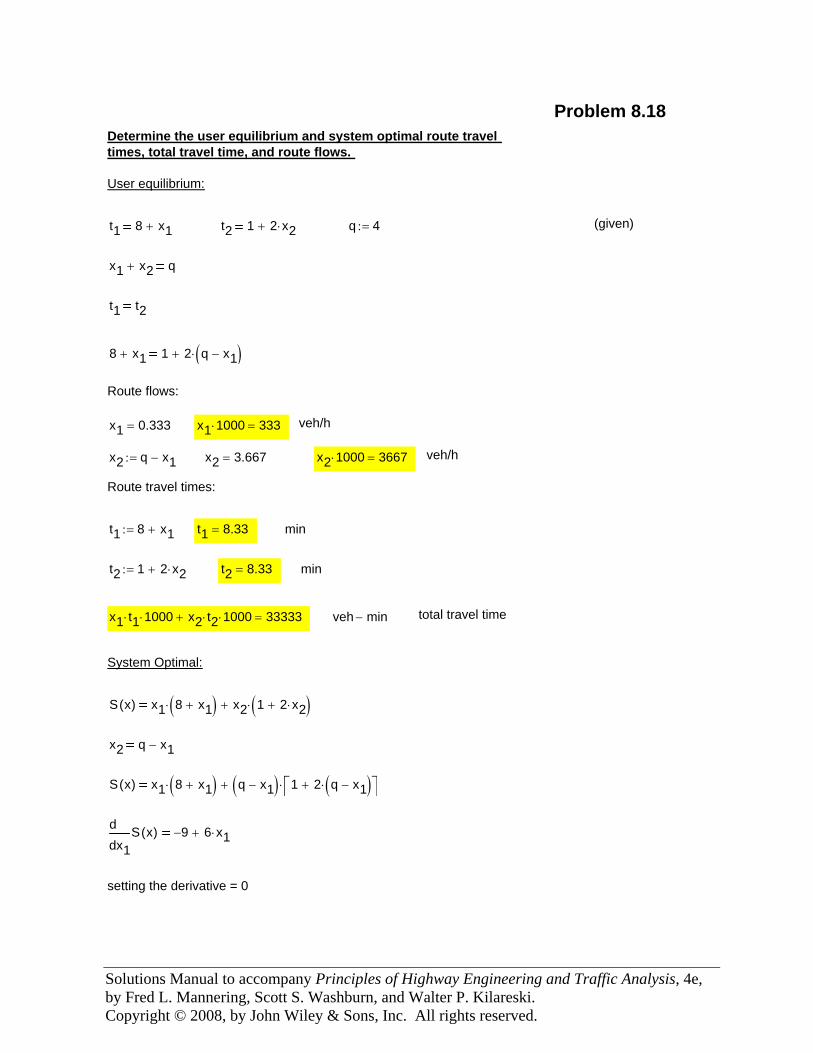
Solutions Manual to accompany Principles of Highway Engineering and Traffic Analysis, 4e, by Fred L. Mannering, Scott S. Washburn, and Walter P. Kilareski. Copyright © 2008, by John Wiley & Sons, Inc. All rights reserved.
x2 1000⋅ 3667= veh/h
Route travel times:
t1 8 x1+:= t1 8.33= min
t2 1 2 x2⋅+:= t2 8.33= min
x1 t1⋅ 1000⋅ x2 t2⋅ 1000⋅+ 33333= veh min− total travel time
System Optimal:
S x( ) x1 8 x1+( )⋅ x2 1 2 x2⋅+( )⋅+
x2 q x1−
S x( ) x1 8 x1+( )⋅ q x1−( ) 1 2 q x1−( )⋅+⎡⎣ ⎤⎦⋅+
x1S x( )d
d9− 6 x1⋅+
setting the derivative = 0
Problem 8.18Determine the user equilibrium and system optimal route travel times, total travel time, and route flows.
User equilibrium:
t1 8 x1+ t2 1 2 x2⋅+ q 4:= (given)
x1 x2+ q
t1 t2
8 x1+ 1 2 q x1−( )⋅+
Route flows:
x1 0.333= x1 1000⋅ 333= veh/h
x2 q x1−:= x2 3.667=
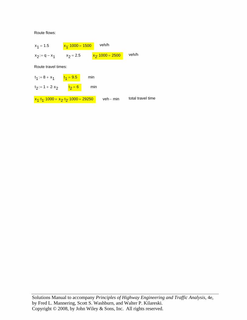
Solutions Manual to accompany Principles of Highway Engineering and Traffic Analysis, 4e, by Fred L. Mannering, Scott S. Washburn, and Walter P. Kilareski. Copyright © 2008, by John Wiley & Sons, Inc. All rights reserved.
total travel timeveh min−x1 t1⋅ 1000⋅ x2 t2⋅ 1000⋅+ 29250=
mint2 6=t2 1 2 x2⋅+:=
mint1 9.5=t1 8 x1+:=
Route travel times:
veh/hx2 1000⋅ 2500=x2 2.5=x2 q x1−:=
veh/hx1 1000⋅ 1500=x1 1.5=
Route flows:
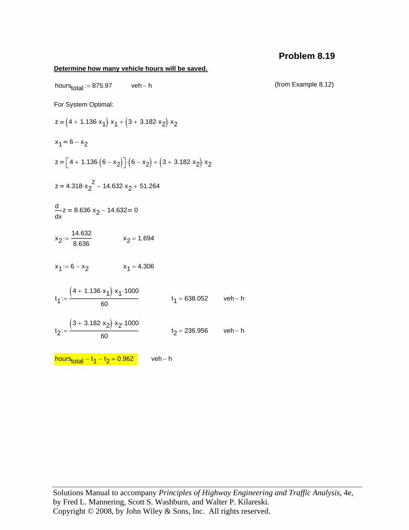
Solutions Manual to accompany Principles of Highway Engineering and Traffic Analysis, 4e, by Fred L. Mannering, Scott S. Washburn, and Walter P. Kilareski. Copyright © 2008, by John Wiley & Sons, Inc. All rights reserved.
veh h−hourstotal t1− t2− 0.962=
veh h−t2 236.956=t23 3.182 x2⋅+( ) x2⋅ 1000⋅
60:=
veh h−t1 638.052=t14 1.136 x1⋅+( ) x1⋅ 1000⋅
60:=
x1 4.306=x1 6 x2−:=
x2 1.694=x214.6328.636
:=
xzd
d8.636 x2⋅ 14.632− 0
z 4.318 x22
⋅ 14.632 x2⋅− 51.264+
z 4 1.136 6 x2−( )⋅+⎡⎣ ⎤⎦ 6 x2−( )⋅ 3 3.182 x2⋅+( ) x2⋅+
x1 6 x2−
z 4 1.136 x1⋅+( ) x1⋅ 3 3.182 x2⋅+( ) x2⋅+
For System Optimal:
(from Example 8.12)veh h−hourstotal 875.97:=
Determine how many vehicle hours will be saved.
Problem 8.19
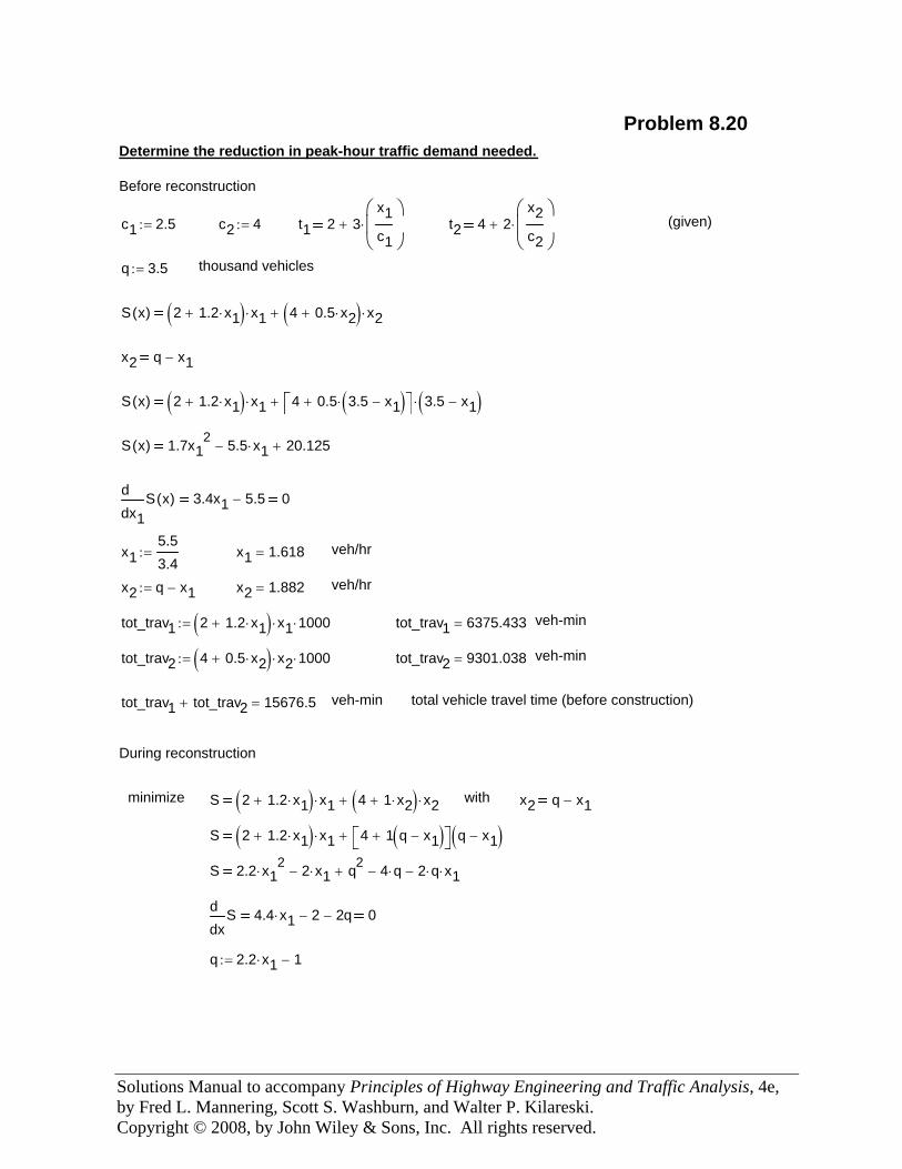
Solutions Manual to accompany Principles of Highway Engineering and Traffic Analysis, 4e, by Fred L. Mannering, Scott S. Washburn, and Walter P. Kilareski. Copyright © 2008, by John Wiley & Sons, Inc. All rights reserved.
veh/hr
tot_trav1 2 1.2 x1⋅+( ) x1⋅ 1000⋅:= tot_trav1 6375.433= veh-min
tot_trav2 4 0.5 x2⋅+( ) x2⋅ 1000⋅:= tot_trav2 9301.038= veh-min
tot_trav1 tot_trav2+ 15676.5= veh-min total vehicle travel time (before construction)
During reconstruction
minimize S 2 1.2 x1⋅+( ) x1⋅ 4 1 x2⋅+( ) x2⋅+ with x2 q x1−
S 2 1.2 x1⋅+( ) x1⋅ 4 1 q x1−( )+⎡⎣ ⎤⎦ q x1−( )+
S 2.2 x12
⋅ 2 x1⋅− q2+ 4 q⋅− 2 q⋅ x1⋅−
xSd
d4.4 x1⋅ 2− 2q− 0
q 2.2 x1⋅ 1−:=
Problem 8.20Determine the reduction in peak-hour traffic demand needed.
Before reconstruction
c1 2.5:= c2 4:= t1 2 3x1c1
⎛⎜⎜⎝
⎞⎟⎟⎠
⋅+ t2 4 2x2c2
⎛⎜⎜⎝
⎞⎟⎟⎠
⋅+ (given)
q 3.5:= thousand vehicles
S x( ) 2 1.2 x1⋅+( ) x1⋅ 4 0.5 x2⋅+( ) x2⋅+
x2 q x1−
S x( ) 2 1.2 x1⋅+( ) x1⋅ 4 0.5 3.5 x1−( )⋅+⎡⎣ ⎤⎦ 3.5 x1−( )⋅+
S x( ) 1.7x12 5.5 x1⋅− 20.125+
x1S x( )d
d3.4x1 5.5− 0
x15.53.4
:= x1 1.618= veh/hr
x2 q x1−:= x2 1.882=
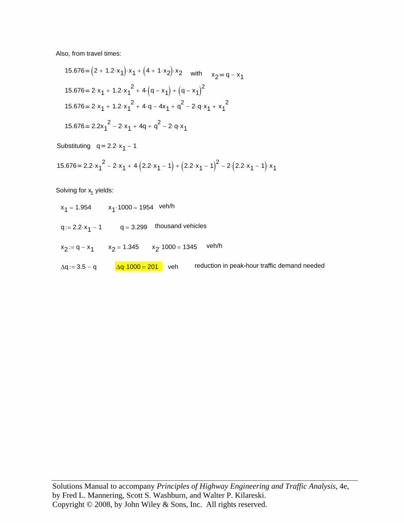
Solutions Manual to accompany Principles of Highway Engineering and Traffic Analysis, 4e, by Fred L. Mannering, Scott S. Washburn, and Walter P. Kilareski. Copyright © 2008, by John Wiley & Sons, Inc. All rights reserved.
reduction in peak-hour traffic demand neededvehΔq 1000⋅ 201=Δq 3.5 q−:=
veh/hx2 1000⋅ 1345=x2 1.345=x2 q x1−:=
thousand vehiclesq 3.299=q 2.2 x1⋅ 1−:=
veh/hx1 1000⋅ 1954=x1 1.954=
Solving for x1 yields:
15.676 2.2 x12
⋅ 2 x1⋅− 4 2.2 x1⋅ 1−( )⋅+ 2.2 x1⋅ 1−( )2+ 2 2.2 x1⋅ 1−( )⋅ x1⋅−
q 2.2 x1⋅ 1−Substituting
15.676 2.2x12 2 x1⋅− 4q+ q2
+ 2 q⋅ x1⋅−
15.676 2 x1⋅ 1.2 x12
⋅+ 4 q⋅+ 4x1− q2+ 2 q⋅ x1⋅− x1
2+
15.676 2 x1⋅ 1.2 x12
⋅+ 4 q x1−( )⋅+ q x1−( )2+
x2 q x1−with15.676 2 1.2 x1⋅+( ) x1⋅ 4 1 x2⋅+( ) x2⋅+
Also, from travel times:
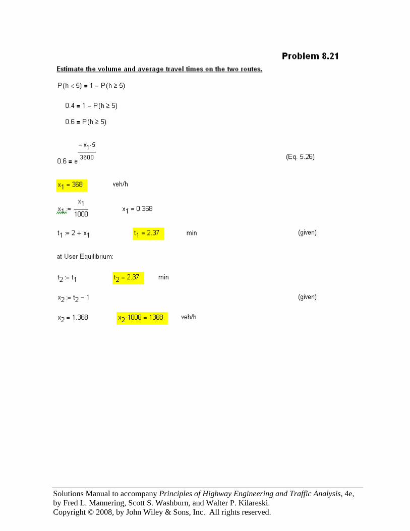
Solutions Manual to accompany Principles of Highway Engineering and Traffic Analysis, 4e, by Fred L. Mannering, Scott S. Washburn, and Walter P. Kilareski. Copyright © 2008, by John Wiley & Sons, Inc. All rights reserved.
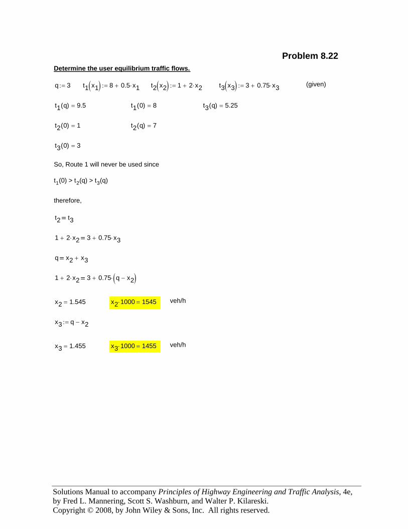
Solutions Manual to accompany Principles of Highway Engineering and Traffic Analysis, 4e, by Fred L. Mannering, Scott S. Washburn, and Walter P. Kilareski. Copyright © 2008, by John Wiley & Sons, Inc. All rights reserved.
veh/hx3 1000⋅ 1455=x3 1.455=
x3 q x2−:=
veh/hx2 1000⋅ 1545=x2 1.545=
1 2 x2⋅+ 3 0.75 q x2−( )⋅+
q x2 x3+
1 2 x2⋅+ 3 0.75 x3⋅+
t2 t3
therefore,
So, Route 1 will never be used since
t1(0) > t2(q) > t3(q)
t3 0( ) 3=
t2 q( ) 7=t2 0( ) 1=
t3 q( ) 5.25=t1 0( ) 8=t1 q( ) 9.5=
(given)t3 x3( ) 3 0.75 x3⋅+:=t2 x2( ) 1 2 x2⋅+:=t1 x1( ) 8 0.5 x1⋅+:=q 3:=
Determine the user equilibrium traffic flows.
Problem 8.22
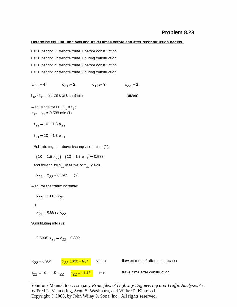
Solutions Manual to accompany Principles of Highway Engineering and Traffic Analysis, 4e, by Fred L. Mannering, Scott S. Washburn, and Walter P. Kilareski. Copyright © 2008, by John Wiley & Sons, Inc. All rights reserved.
x21 x22 0.392− 2( )
Also, for the traffic increase:
x22 1.685 x21⋅
or
x21 0.5935 x22⋅
Substituting into (2):
0.5935 x22⋅ x22 0.392−
x22 0.964= x22 1000⋅ 964= veh/h flow on route 2 after construction
t22 10 1.5 x22⋅+:= t22 11.45= min travel time after construction
Problem 8.23
Determine equilibrium flows and travel times before and after reconstruction begins.
Let subscript 11 denote route 1 before construction
Let subscript 12 denote route 1 during construction
Let subscript 21 denote route 2 before construction
Let subscript 22 denote route 2 during construction
c11 4:= c21 2:= c12 3:= c22 2:=
t12 - t11 = 35.28 s or 0.588 min (given)
Also, since for UE, t 1 = t 2; t22 - t21 = 0.588 min (1)
t22 10 1.5 x22⋅+
t21 10 1.5 x21⋅+
Substituting the above two equations into (1):
10 1.5 x22⋅+( ) 10 1.5 x21⋅+( )− 0.588
and solving for x21 in terms of x22 yields:
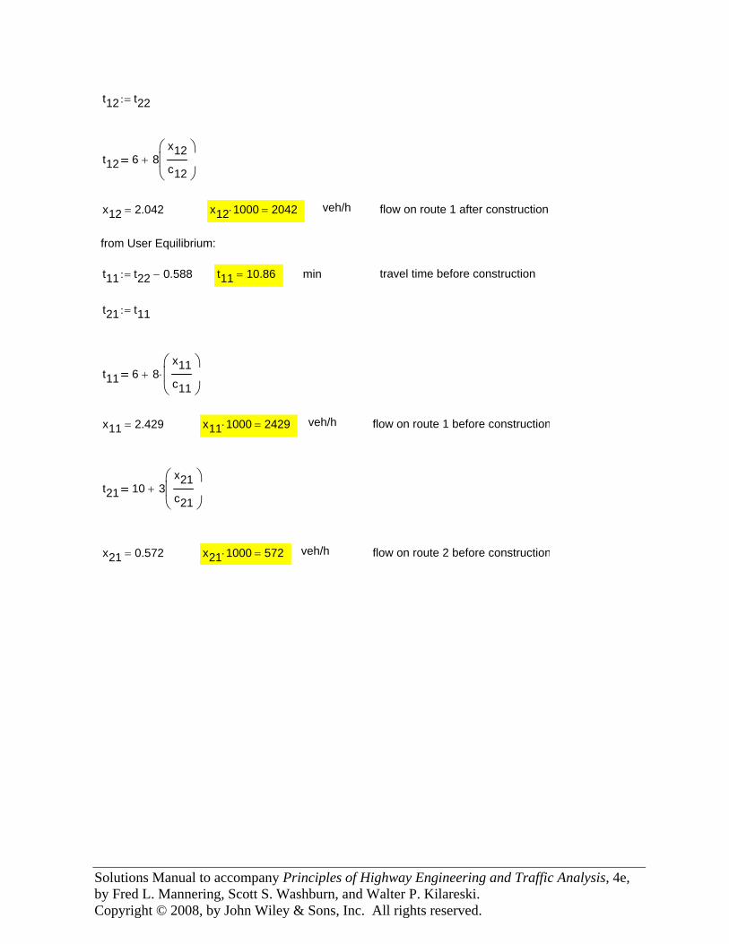
Solutions Manual to accompany Principles of Highway Engineering and Traffic Analysis, 4e, by Fred L. Mannering, Scott S. Washburn, and Walter P. Kilareski. Copyright © 2008, by John Wiley & Sons, Inc. All rights reserved.
flow on route 2 before constructionveh/hx21 1000⋅ 572=x21 0.572=
t21 10 3x21c21
⎛⎜⎜⎝
⎞⎟⎟⎠
+
flow on route 1 before constructionveh/hx11 1000⋅ 2429=x11 2.429=
t11 6 8x11c11
⎛⎜⎜⎝
⎞⎟⎟⎠
⋅+
t21 t11:=
travel time before constructionmint11 10.86=t11 t22 0.588−:=
from User Equilibrium:
flow on route 1 after constructionveh/hx12 1000⋅ 2042=x12 2.042=
t12 6 8x12c12
⎛⎜⎜⎝
⎞⎟⎟⎠
+
t12 t22:=
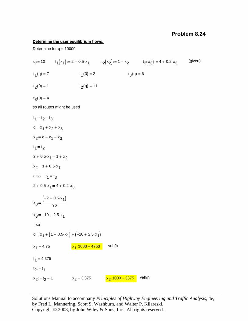
Solutions Manual to accompany Principles of Highway Engineering and Traffic Analysis, 4e, by Fred L. Mannering, Scott S. Washburn, and Walter P. Kilareski. Copyright © 2008, by John Wiley & Sons, Inc. All rights reserved.
x2 1 0.5 x1⋅+
also t1 t3
2 0.5 x1⋅+ 4 0.2 x3⋅+
x32− 0.5 x1⋅+( )
0.2
x3 10− 2.5 x1⋅+
so
q x1 1 0.5 x1⋅+( )+ 10− 2.5 x1⋅+( )+
x1 4.75= x1 1000⋅ 4750= veh/h
t1 4.375=
t2 t1:=
x2 t2 1−:= x2 3.375= x2 1000⋅ 3375= veh/h
Problem 8.24Determine the user equilibrium flows.
Determine for q = 10000
q 10:= t1 x1( ) 2 0.5 x1⋅+:= t2 x2( ) 1 x2+:= t3 x3( ) 4 0.2 x3⋅+:= (given)
t1 q( ) 7= t1 0( ) 2= t3 q( ) 6=
t2 0( ) 1= t2 q( ) 11=
t3 0( ) 4=
so all routes might be used
t1 t2 t3
q x1 x2+ x3+
x2 q x1− x3−
t1 t2
2 0.5 x1⋅+ 1 x2+
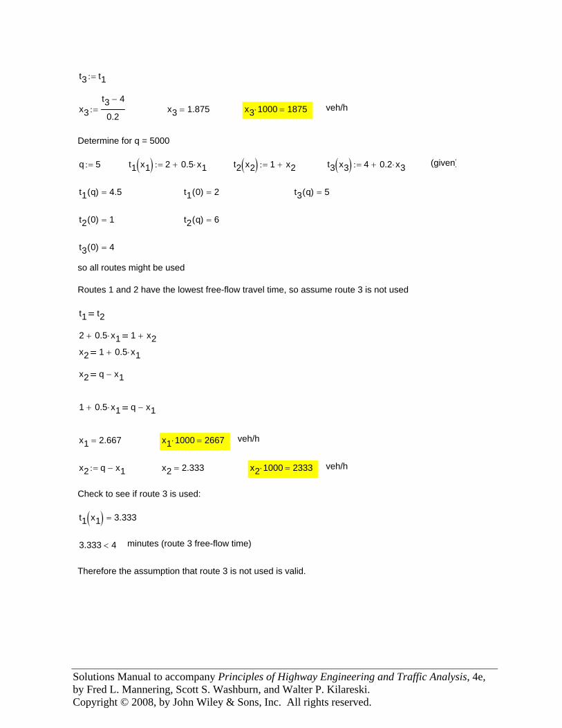
Solutions Manual to accompany Principles of Highway Engineering and Traffic Analysis, 4e, by Fred L. Mannering, Scott S. Washburn, and Walter P. Kilareski. Copyright © 2008, by John Wiley & Sons, Inc. All rights reserved.
t1 t2
2 0.5 x1⋅+ 1 x2+
x2 1 0.5 x1⋅+
x2 q x1−
1 0.5 x1⋅+ q x1−
x1 2.667= x1 1000⋅ 2667= veh/h
x2 q x1−:= x2 2.333= x2 1000⋅ 2333= veh/h
Check to see if route 3 is used:
t1 x1( ) 3.333=
3.333 4< minutes (route 3 free-flow time)
Therefore the assumption that route 3 is not used is valid.
t3 t1:=
x3t3 4−
0.2:= x3 1.875= x3 1000⋅ 1875= veh/h
Determine for q = 5000
q 5:= t1 x1( ) 2 0.5 x1⋅+:= t2 x2( ) 1 x2+:= t3 x3( ) 4 0.2 x3⋅+:= (given)
t1 q( ) 4.5= t1 0( ) 2= t3 q( ) 5=
t2 0( ) 1= t2 q( ) 6=
t3 0( ) 4=
so all routes might be used
Routes 1 and 2 have the lowest free-flow travel time, so assume route 3 is not used
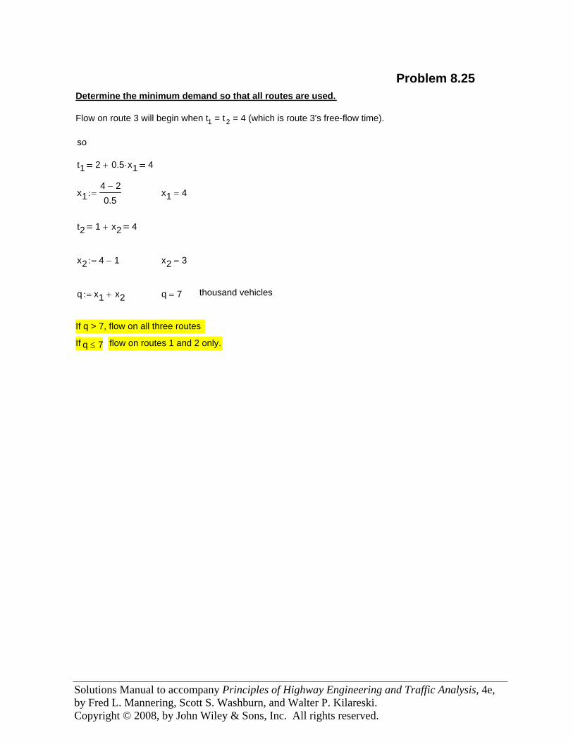
Solutions Manual to accompany Principles of Highway Engineering and Traffic Analysis, 4e, by Fred L. Mannering, Scott S. Washburn, and Walter P. Kilareski. Copyright © 2008, by John Wiley & Sons, Inc. All rights reserved.
flow on routes 1 and 2 only.q 7≤If
If q > 7, flow on all three routes
thousand vehiclesq 7=q x1 x2+:=
x2 3=x2 4 1−:=
t2 1 x2+ 4
x1 4=x14 2−
0.5:=
t1 2 0.5 x1⋅+ 4
so
Flow on route 3 will begin when t1 = t 2 = 4 (which is route 3's free-flow time).
Determine the minimum demand so that all routes are used.
Problem 8.25
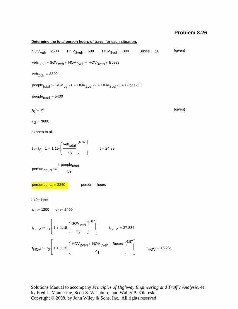
Solutions Manual to accompany Principles of Highway Engineering and Traffic Analysis, 4e, by Fred L. Mannering, Scott S. Washburn, and Walter P. Kilareski. Copyright © 2008, by John Wiley & Sons, Inc. All rights reserved.
Problem 8.26
tHOV 16.261=tHOV t0 1 1.15HOV2veh HOV3veh+ Buses+
c1
⎛⎜⎜⎝
⎞⎟⎟⎠
6.87
⋅+
⎡⎢⎢⎣
⎤⎥⎥⎦
⋅:=
tSOV 37.834=tSOV t0 1 1.15SOVveh
c2
⎛⎜⎜⎝
⎞⎟⎟⎠
6.87
⋅+
⎡⎢⎢⎣
⎤⎥⎥⎦
⋅:=
c2 2400:=c1 1200:=
b) 2+ lane
person hours−personhours 2240=
personhourst peopletotal⋅
60:=
t 24.89=t t0 1 1.15vehtotal
c3
⎛⎜⎜⎝
⎞⎟⎟⎠
6.87
⋅+
⎡⎢⎢⎣
⎤⎥⎥⎦
⋅:=
a) open to all
c3 3600:=
(given)t0 15:=
peopletotal 5400=
peopletotal SOVveh 1⋅ HOV2veh 2⋅+ HOV3veh 3⋅+ Buses 50⋅+:=
vehtotal 3320=
vehtotal SOVveh HOV2veh+ HOV3veh+ Buses+:=
(given)Buses 20:=HOV3veh 300:=HOV2veh 500:=SOVveh 2500:=
Determine the total person hours of travel for each situation.
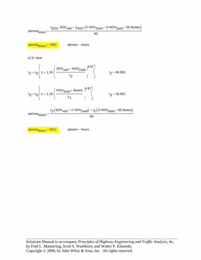
Solutions Manual to accompany Principles of Highway Engineering and Traffic Analysis, 4e, by Fred L. Mannering, Scott S. Washburn, and Walter P. Kilareski. Copyright © 2008, by John Wiley & Sons, Inc. All rights reserved.
personhourstSOV SOVveh⋅ tHOV 2 HOV2veh⋅ 3 HOV3veh⋅+ 50 Buses⋅+( )⋅+
60:=
personhours 2362= person hours−
c) 3+ lane
t2 t0 1 1.15SOVveh HOV2veh+
c2
⎛⎜⎜⎝
⎞⎟⎟⎠
6.87
⋅+
⎡⎢⎢⎣
⎤⎥⎥⎦
⋅:= t2 94.903=
t3 t0 1 1.15HOV3veh Buses+
c1
⎛⎜⎜⎝
⎞⎟⎟⎠
6.87
⋅+
⎡⎢⎢⎣
⎤⎥⎥⎦
⋅:= t3 15.002=
personhourst2 SOVveh 2 HOV2veh⋅+( )⋅ t3 3 HOV3veh⋅ 50 Buses⋅+( )⋅+
60:=
personhours 6011= person hours−
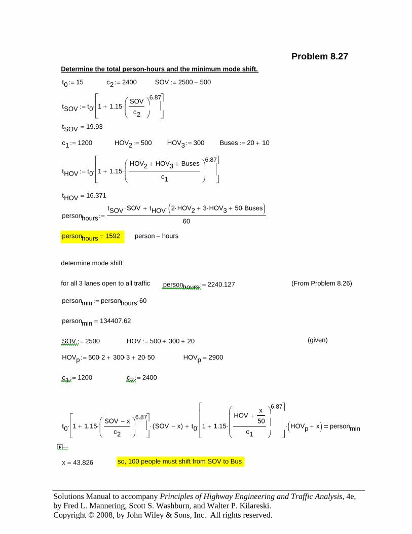
Solutions Manual to accompany Principles of Highway Engineering and Traffic Analysis, 4e, by Fred L. Mannering, Scott S. Washburn, and Walter P. Kilareski. Copyright © 2008, by John Wiley & Sons, Inc. All rights reserved.
Problem 8.27Determine the total person-hours and the minimum mode shift.
t0 15:= c2 2400:= SOV 2500 500−:=
tSOV t0 1 1.15SOVc2
⎛⎜⎝
⎞⎟⎠
6.87⋅+
⎡⎢⎢⎣
⎤⎥⎥⎦
⋅:=
tSOV 19.93=
c1 1200:= HOV2 500:= HOV3 300:= Buses 20 10+:=
tHOV t0 1 1.15HOV2 HOV3+ Buses+
c1
⎛⎜⎜⎝
⎞⎟⎟⎠
6.87
⋅+
⎡⎢⎢⎣
⎤⎥⎥⎦
⋅:=
tHOV 16.371=
personhourstSOV SOV⋅ tHOV 2 HOV2⋅ 3 HOV3⋅+ 50 Buses⋅+( )⋅+
60:=
personhours 1592= person hours−
determine mode shift
for all 3 lanes open to all traffic personhours 2240.127:= (From Problem 8.26)
personmin personhours 60⋅:=
personmin 134407.62=
SOV 2500:= HOV 500 300+ 20+:= (given)
HOVp 500 2⋅ 300 3⋅+ 20 50⋅+:= HOVp 2900=
c1 1200:= c2 2400:=
t0 1 1.15SOV x−
c2
⎛⎜⎝
⎞⎟⎠
6.87⋅+
⎡⎢⎢⎣
⎤⎥⎥⎦
⋅ SOV x−( )⋅ t0 1 1.15HOV
x50
+
c1
⎛⎜⎜⎜⎝
⎞⎟⎟⎟⎠
6.87
⋅+
⎡⎢⎢⎢⎣
⎤⎥⎥⎥⎦
⋅ HOVp x+( )⋅+ personmin
x 43.826= so, 100 people must shift from SOV to Bus
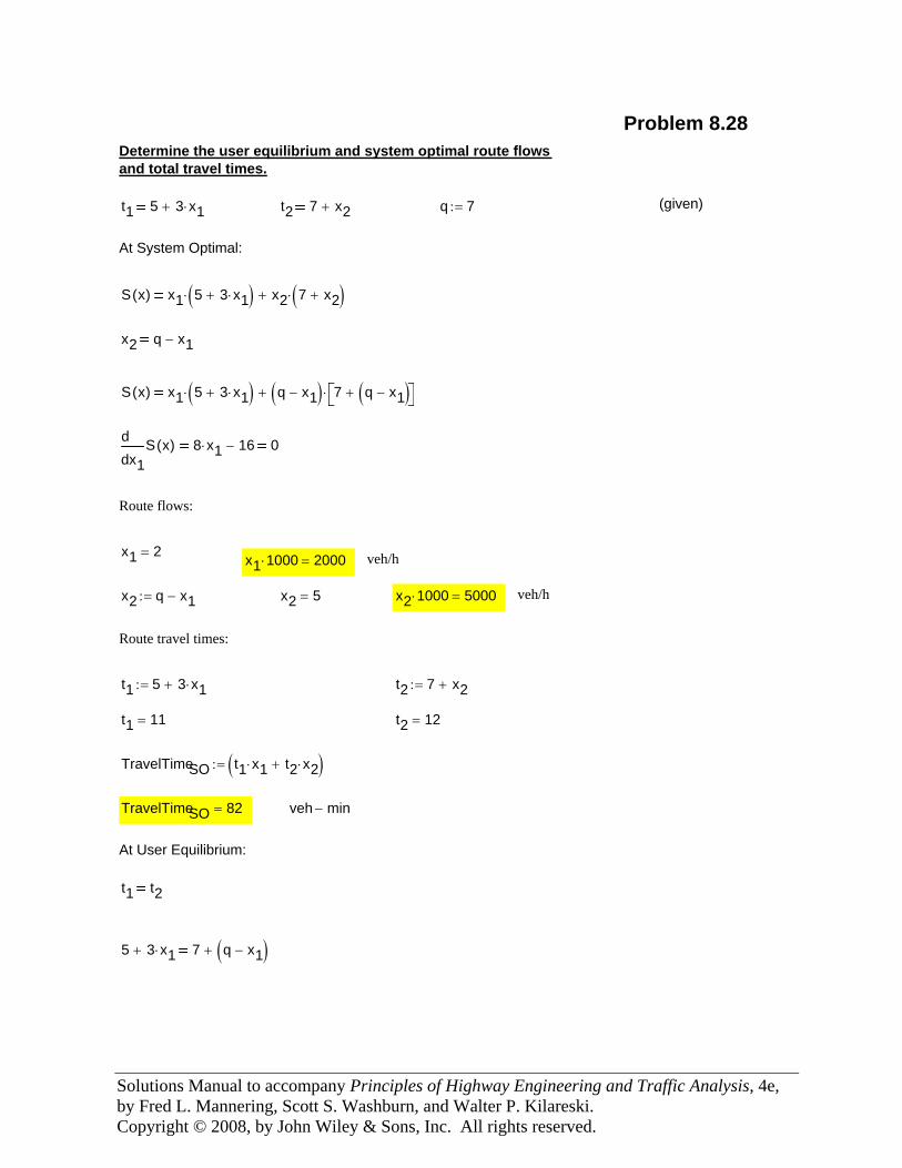
Solutions Manual to accompany Principles of Highway Engineering and Traffic Analysis, 4e, by Fred L. Mannering, Scott S. Washburn, and Walter P. Kilareski. Copyright © 2008, by John Wiley & Sons, Inc. All rights reserved.
5 3 x1⋅+ 7 q x1−( )+
t1 t2
At User Equilibrium:
veh min−TravelTimeSO 82=
TravelTimeSO t1 x1⋅ t2 x2⋅+( ):=
t2 12=t1 11=
t2 7 x2+:=t1 5 3 x1⋅+:=
Route travel times:
veh/hx2 1000⋅ 5000=x2 5=
Problem 8.28Determine the user equilibrium and system optimal route flowsand total travel times.
t1 5 3 x1⋅+ t2 7 x2+ q 7:= (given)
At System Optimal:
S x( ) x1 5 3 x1⋅+( )⋅ x2 7 x2+( )⋅+
x2 q x1−
S x( ) x1 5 3 x1⋅+( )⋅ q x1−( ) 7 q x1−( )+⎡⎣ ⎤⎦⋅+
x1S x( )d
d8 x1⋅ 16− 0
Route flows:
x1 2= x1 1000⋅ 2000= veh/h
x2 q x1−:=
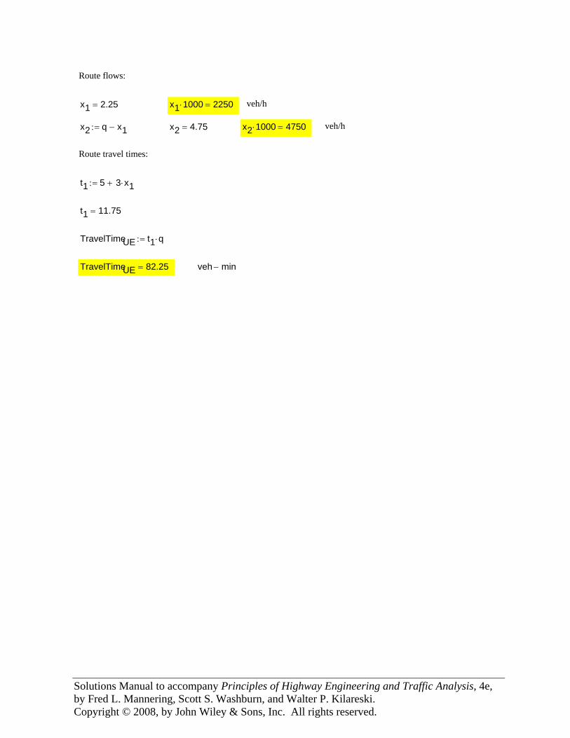
Solutions Manual to accompany Principles of Highway Engineering and Traffic Analysis, 4e, by Fred L. Mannering, Scott S. Washburn, and Walter P. Kilareski. Copyright © 2008, by John Wiley & Sons, Inc. All rights reserved.
Route flows:
x1 2.25= x1 1000⋅ 2250= veh/h
x2 q x1−:= x2 4.75= x2 1000⋅ 4750= veh/h
Route travel times:
t1 5 3 x1⋅+:=
t1 11.75=
TravelTimeUE t1 q⋅:=
TravelTimeUE 82.25= veh min−
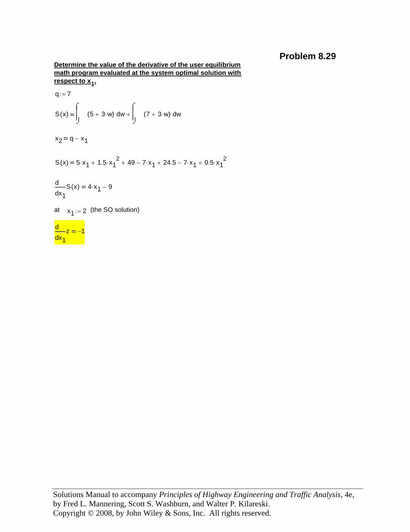
Solutions Manual to accompany Principles of Highway Engineering and Traffic Analysis, 4e, by Fred L. Mannering, Scott S. Washburn, and Walter P. Kilareski. Copyright © 2008, by John Wiley & Sons, Inc. All rights reserved.
Problem 8.29Determine the value of the derivative of the user equilibriummath program evaluated at the system optimal solution withrespect to x1.
q 7:=
S x( ) w5 3 w⋅+( )⌠⎮⎮⌡
d w7 3 w⋅+( )⌠⎮⎮⌡
d+
x2 q x1−
S x( ) 5 x1⋅ 1.5 x12
⋅+ 49+ 7 x1⋅− 24.5+ 7 x1⋅− 0.5 x12
⋅+
x1S x( )d
d4 x1⋅ 9−
at x1 2:= (the SO solution)
x1zd
d1−
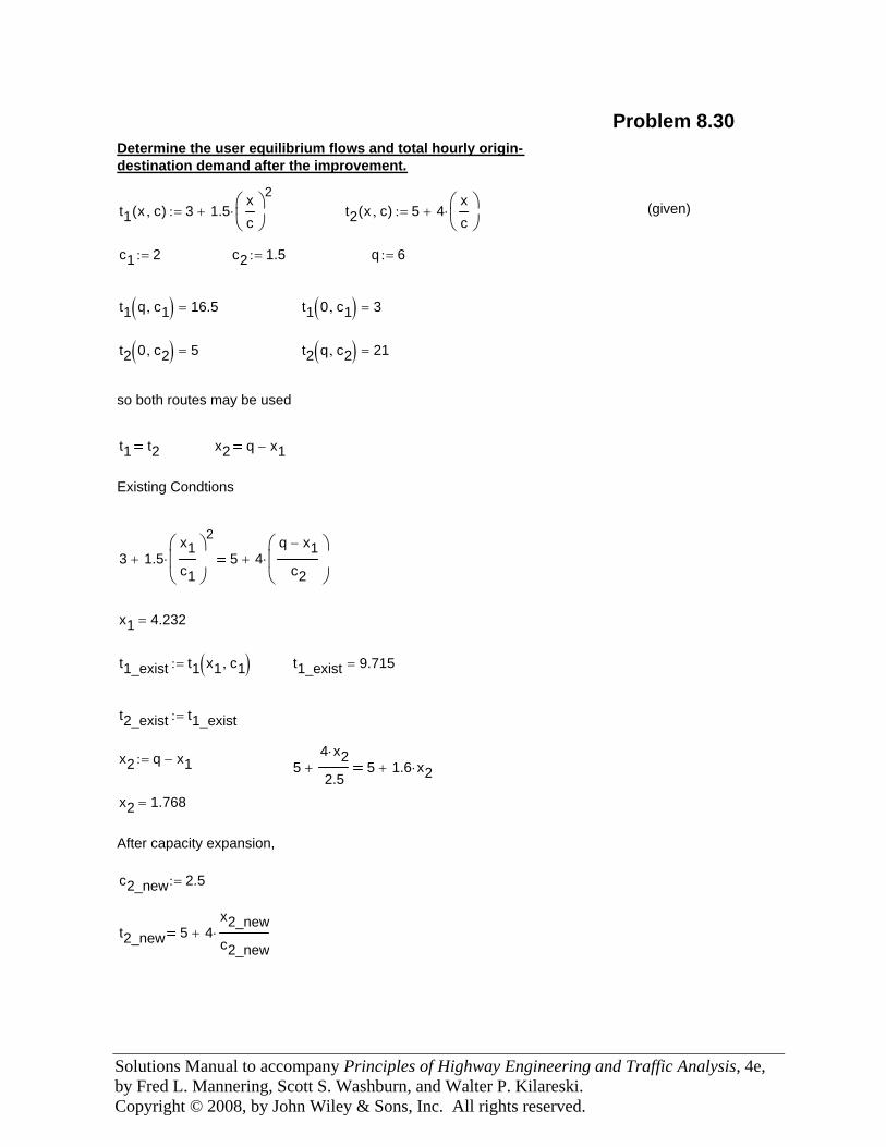
Solutions Manual to accompany Principles of Highway Engineering and Traffic Analysis, 4e, by Fred L. Mannering, Scott S. Washburn, and Walter P. Kilareski. Copyright © 2008, by John Wiley & Sons, Inc. All rights reserved.
t2_new 5 4
x2_newc2_new⋅+
c2_new 2.5:=
After capacity expansion,
x2 1.768=
54 x2⋅
2.5+ 5 1.6 x2⋅+
x2 q x1−:=
t2_exist t1_exist:=
t1_exist 9.715=t1_exist t1 x1 c1,( ):=
x1 4.232=
3 1.5x1c1
⎛⎜⎜⎝
⎞⎟⎟⎠
2
⋅+ 5 4q x1−
c2
⎛⎜⎜⎝
⎞⎟⎟⎠
⋅+
Existing Condtions
x2 q x1−t1 t2
so both routes may be used
t2 q c2,( ) 21=t2 0 c2,( ) 5=
t1 0 c1,( ) 3=t1 q c1,( ) 16.5=
q 6:=c2 1.5:=c1 2:=
(given)t2 x c,( ) 5 4xc
⎛⎜⎝
⎞⎟⎠
⋅+:=t1 x c,( ) 3 1.5xc
⎛⎜⎝
⎞⎟⎠
2⋅+:=
Determine the user equilibrium flows and total hourly origin-destination demand after the improvement.
Problem 8.30
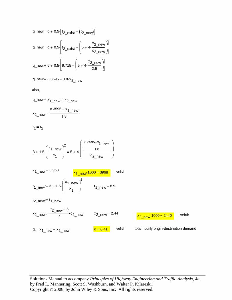
Solutions Manual to accompany Principles of Highway Engineering and Traffic Analysis, 4e, by Fred L. Mannering, Scott S. Washburn, and Walter P. Kilareski. Copyright © 2008, by John Wiley & Sons, Inc. All rights reserved.
total hourly origin-destination demandveh/hq 6.41=q x1_new x2_new+:=
veh/hx2_new 1000⋅ 2440=x2_new 2.44=x2_new
t2_new 5−
4c2_new⋅:=
t2_new t1_new:=
t1_new 8.9=t1_new 3 1.5x1_new
c1
⎛⎜⎜⎝
⎞⎟⎟⎠
2
⋅+:=
veh/hx1_new 1000⋅ 3968=x1_new 3.968=
3 1.5x1_new
c1
⎛⎜⎜⎝
⎞⎟⎟⎠
2
⋅+ 5 4
8.3595 x1_new−
1.8
c2_new
⎛⎜⎜⎜⎝
⎞⎟⎟⎟⎠
⋅+
t1 t2
x2_new8.3595 x1_new−
1.8
q_new x1_new x2_new+
also,
q_new 8.3595 0.8 x2_new⋅−
q_new 6 0.5 9.715 5 4x2_new
2.5⋅+
⎛⎜⎝
⎞⎟⎠
−⎡⎢⎣
⎤⎥⎦
⋅+
q_new q 0.5 t2_exist 5 4x2_newc2_new⋅+
⎛⎜⎜⎝
⎞⎟⎟⎠
−⎡⎢⎢⎣
⎤⎥⎥⎦
⋅+
q_new q 0.5 t2_exist t2_new( )−⎡⎣ ⎤⎦⋅+
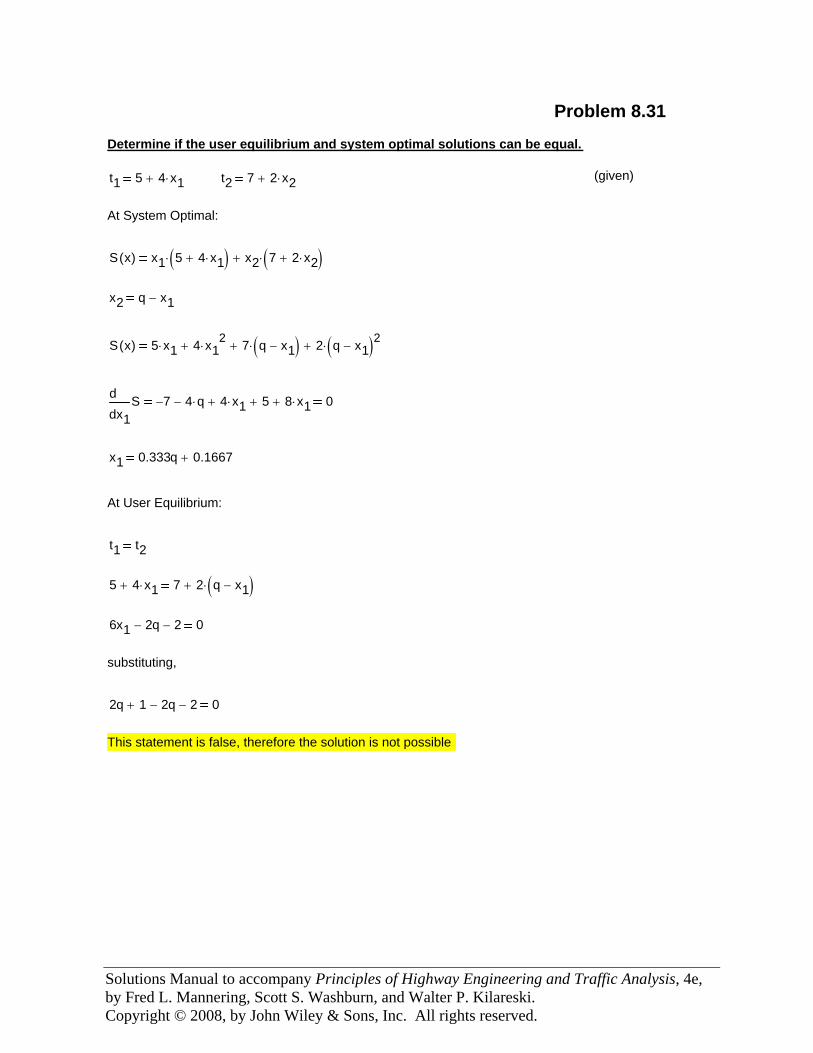
Solutions Manual to accompany Principles of Highway Engineering and Traffic Analysis, 4e, by Fred L. Mannering, Scott S. Washburn, and Walter P. Kilareski. Copyright © 2008, by John Wiley & Sons, Inc. All rights reserved.
This statement is false, therefore the solution is not possible
2q 1+ 2q− 2− 0
substituting,
6x1 2q− 2− 0
5 4 x1⋅+ 7 2 q x1−( )⋅+
t1 t2
At User Equilibrium:
x1 0.333q 0.1667+
x1Sd
d7− 4 q⋅− 4 x1⋅+ 5+ 8 x1⋅+ 0
S x( ) 5 x1⋅ 4 x12
⋅+ 7 q x1−( )⋅+ 2 q x1−( )2⋅+
x2 q x1−
S x( ) x1 5 4 x1⋅+( )⋅ x2 7 2 x2⋅+( )⋅+
At System Optimal:
(given)t2 7 2 x2⋅+t1 5 4 x1⋅+
Determine if the user equilibrium and system optimal solutions can be equal.
Problem 8.31
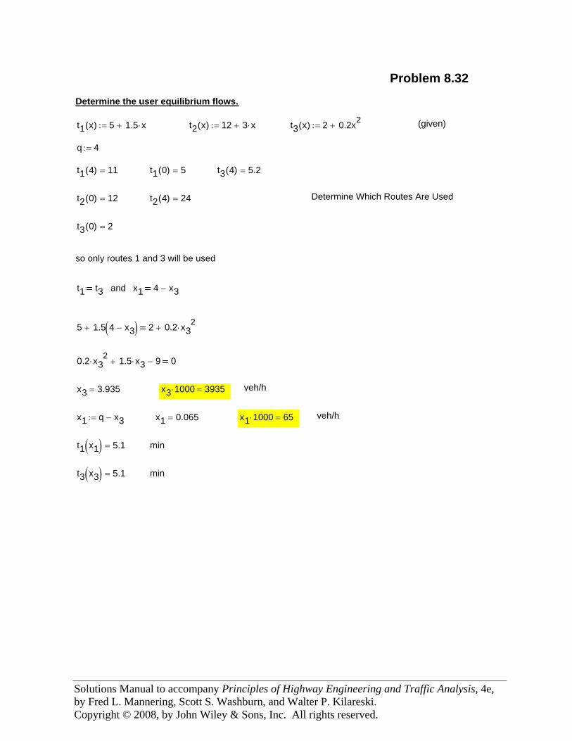
Solutions Manual to accompany Principles of Highway Engineering and Traffic Analysis, 4e, by Fred L. Mannering, Scott S. Washburn, and Walter P. Kilareski. Copyright © 2008, by John Wiley & Sons, Inc. All rights reserved.
mint3 x3( ) 5.1=
mint1 x1( ) 5.1=
veh/hx1 1000⋅ 65=x1 0.065=x1 q x3−:=
veh/hx3 1000⋅ 3935=x3 3.935=
0.2 x32
⋅ 1.5 x3⋅+ 9− 0
5 1.5 4 x3−( )+ 2 0.2 x32
⋅+
x1 4 x3−
Problem 8.32
Determine the user equilibrium flows.
t1 x( ) 5 1.5 x⋅+:= t2 x( ) 12 3 x⋅+:= t3 x( ) 2 0.2x2+:= (given)
q 4:=
t1 4( ) 11= t1 0( ) 5= t3 4( ) 5.2=
t2 0( ) 12= t2 4( ) 24= Determine Which Routes Are Used
t3 0( ) 2=
so only routes 1 and 3 will be used
t1 t3 and
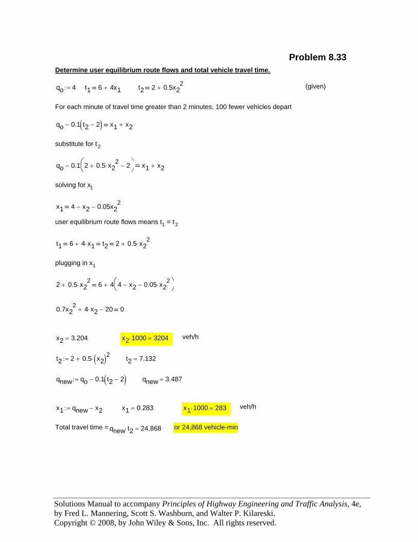
Solutions Manual to accompany Principles of Highway Engineering and Traffic Analysis, 4e, by Fred L. Mannering, Scott S. Washburn, and Walter P. Kilareski. Copyright © 2008, by John Wiley & Sons, Inc. All rights reserved.
or 24,868 vehicle-minqnew t2⋅ 24.868=Total travel time =
veh/hx1 1000⋅ 283=x1 0.283=x1 qnew x2−:=
qnew 3.487=qnew qo 0.1 t2 2−( )−:=
t2 7.132=t2 2 0.5 x2( )2⋅+:=
veh/hx2 1000⋅ 3204=x2 3.204=
0.7x22 4 x2⋅+ 20− 0
Problem 8.33Determine user equilibrium route flows and total vehicle travel time.
qo 4:= t1 6 4x1+ t2 2 0.5x22
+ (given)
For each minute of travel time greater than 2 minutes, 100 fewer vehicles depart
qo 0.1 t2 2−( )− x1 x2+
substitute for t2
qo 0.1 2 0.5 x22
⋅+ 2−⎛⎝
⎞⎠− x1 x2+
solving for x1
x1 4 x2− 0.05x22
−
user equilibrium route flows means t1 = t 2
t1 6 4 x1⋅+ t2 2 0.5 x22
⋅+
plugging in x1
2 0.5 x22
⋅+ 6 4 4 x2− 0.05 x22
⋅−⎛⎝
⎞⎠+
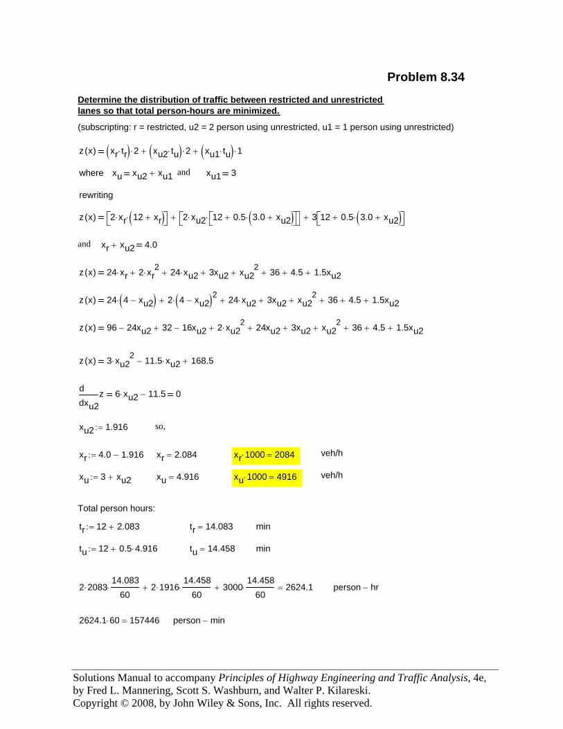
Solutions Manual to accompany Principles of Highway Engineering and Traffic Analysis, 4e, by Fred L. Mannering, Scott S. Washburn, and Walter P. Kilareski. Copyright © 2008, by John Wiley & Sons, Inc. All rights reserved.
Problem 8.34
Determine the distribution of traffic between restricted and unrestrictedlanes so that total person-hours are minimized.
(subscripting: r = restricted, u2 = 2 person using unrestricted, u1 = 1 person using unrestricted)
z x( ) xr tr⋅( ) 2⋅ xu2 tu⋅( ) 2⋅+ xu1 tu⋅( ) 1⋅+
where xu xu2 xu1+ and xu1 3
rewriting
z x( ) 2 xr⋅ 12 xr+( )⋅⎡⎣ ⎤⎦ 2 xu2⋅ 12 0.5 3.0 xu2+( )⋅+⎡⎣ ⎤⎦⋅⎡⎣ ⎤⎦+ 3 12 0.5 3.0 xu2+( )⋅+⎡⎣ ⎤⎦+
and xr xu2+ 4.0
z x( ) 24 xr⋅ 2 xr2
⋅+ 24 xu2⋅+ 3xu2+ xu22
+ 36+ 4.5+ 1.5xu2+
z x( ) 24 4 xu2−( )⋅ 2 4 xu2−( )2⋅+ 24 xu2⋅+ 3xu2+ xu22
+ 36+ 4.5+ 1.5xu2+
z x( ) 96 24xu2− 32+ 16xu2− 2 xu22
⋅+ 24xu2+ 3xu2+ xu22
+ 36+ 4.5+ 1.5xu2+
z x( ) 3 xu22
⋅ 11.5 xu2⋅− 168.5+
xu2zd
d6 xu2⋅ 11.5− 0
xu2 1.916:= so,
xr 4.0 1.916−:= xr 2.084= xr 1000⋅ 2084= veh/h
xu 3 xu2+:= xu 4.916= xu 1000⋅ 4916= veh/h
Total person hours:
tr 12 2.083+:= tr 14.083= min
tu 12 0.5 4.916⋅+:= tu 14.458= min
2 2083⋅14.083
60⋅ 2 1916⋅
14.45860
⋅+ 300014.458
60⋅+ 2624.1= person hr−
2624.1 60⋅ 157446= person min−
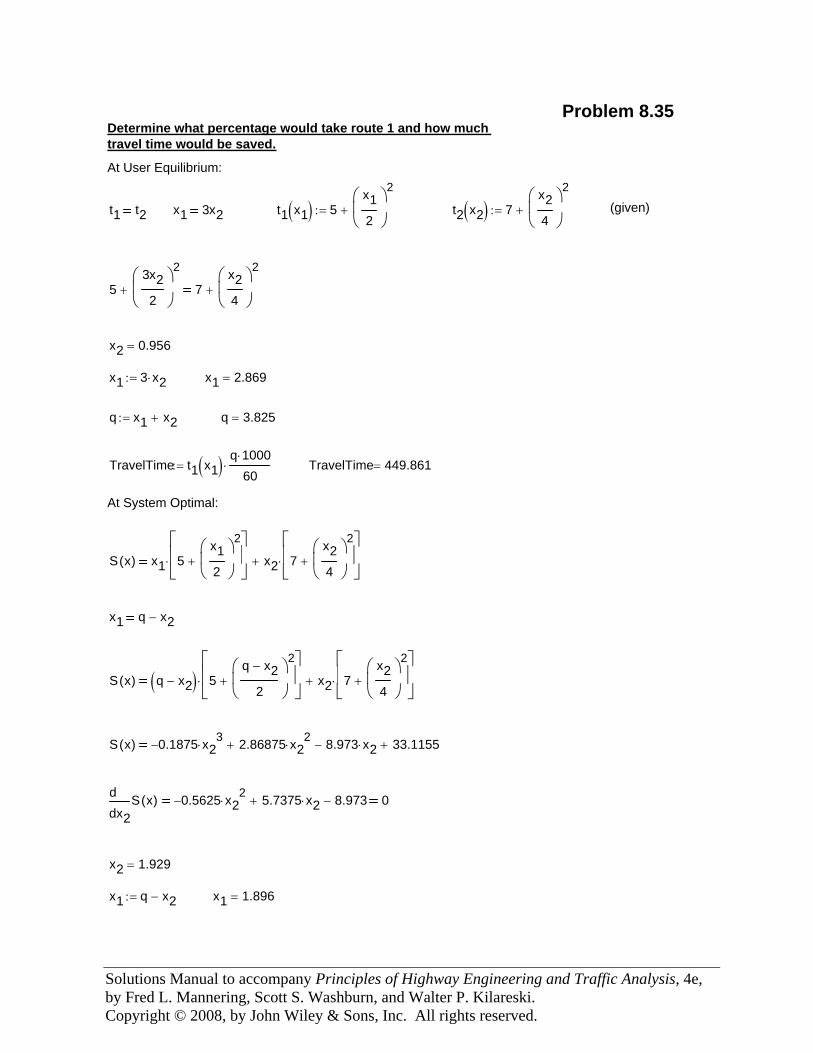
Solutions Manual to accompany Principles of Highway Engineering and Traffic Analysis, 4e, by Fred L. Mannering, Scott S. Washburn, and Walter P. Kilareski. Copyright © 2008, by John Wiley & Sons, Inc. All rights reserved.
x1 1.896=x1 q x2−:=
x2 1.929=
x2S x( )d
d0.5625− x2
2⋅ 5.7375 x2⋅+ 8.973− 0
S x( ) 0.1875− x23
⋅ 2.86875 x22
⋅+ 8.973 x2⋅− 33.1155+
S x( ) q x2−( ) 5q x2−
2
⎛⎜⎝
⎞⎟⎠
2
+
⎡⎢⎢⎣
⎤⎥⎥⎦
⋅ x2 7x24
⎛⎜⎝
⎞⎟⎠
2
+
⎡⎢⎢⎣
⎤⎥⎥⎦
⋅+
x1 q x2−
S x( ) x1 5x12
⎛⎜⎝
⎞⎟⎠
2
+
⎡⎢⎢⎣
⎤⎥⎥⎦
⋅ x2 7x24
⎛⎜⎝
⎞⎟⎠
2
+
⎡⎢⎢⎣
⎤⎥⎥⎦
⋅+
At System Optimal:
TravelTime 449.861=TravelTime t1 x1( ) q 1000⋅
60⋅:=
q 3.825=q x1 x2+:=
x1 2.869=x1 3 x2⋅:=
x2 0.956=
53x22
⎛⎜⎝
⎞⎟⎠
2
+ 7x24
⎛⎜⎝
⎞⎟⎠
2
+
(given)t2 x2( ) 7x24
⎛⎜⎝
⎞⎟⎠
2
+:=t1 x1( ) 5x12
⎛⎜⎝
⎞⎟⎠
2
+:=x1 3x2t1 t2
At User Equilibrium:
Determine what percentage would take route 1 and how muchtravel time would be saved.
Problem 8.35
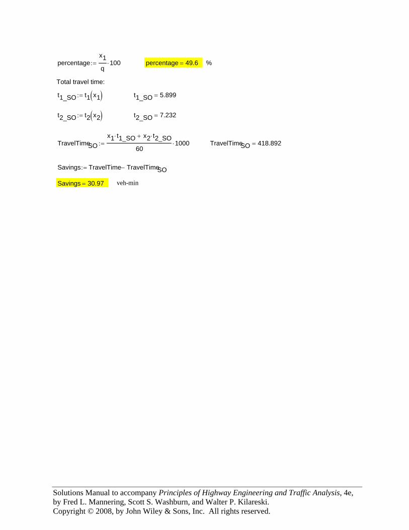
Solutions Manual to accompany Principles of Highway Engineering and Traffic Analysis, 4e, by Fred L. Mannering, Scott S. Washburn, and Walter P. Kilareski. Copyright © 2008, by John Wiley & Sons, Inc. All rights reserved.
percentagex1q
100⋅:= percentage 49.6= %
Total travel time:
t1_SO t1 x1( ):= t1_SO 5.899=
t2_SO t2 x2( ):= t2_SO 7.232=
TravelTimeSOx1 t1_SO⋅ x2 t2_SO⋅+
601000⋅:= TravelTimeSO 418.892=
Savings TravelTime TravelTimeSO−:=
Savings 30.97= veh-min
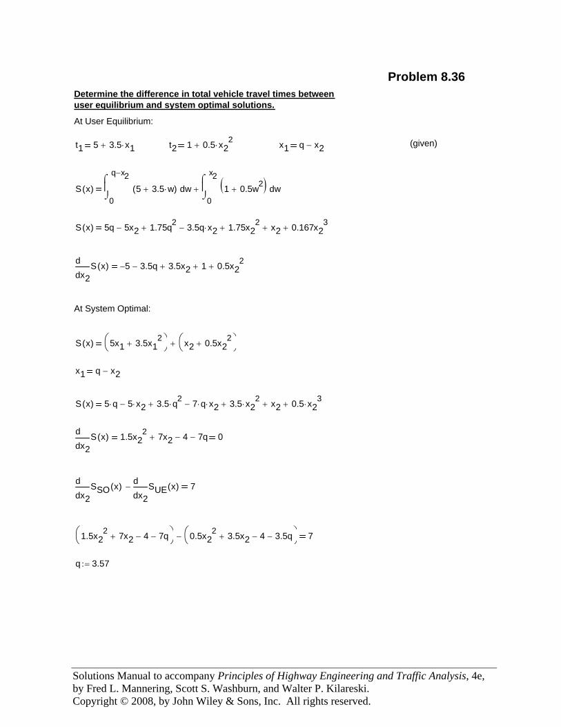
Solutions Manual to accompany Principles of Highway Engineering and Traffic Analysis, 4e, by Fred L. Mannering, Scott S. Washburn, and Walter P. Kilareski. Copyright © 2008, by John Wiley & Sons, Inc. All rights reserved.
q 3.57:=
1.5x22 7x2+ 4− 7q−⎛
⎝⎞⎠ 0.5x2
2 3.5x2+ 4− 3.5q−⎛⎝
⎞⎠− 7
x2SSO x( )d
d x2SUE x( )d
d− 7
x2S x( )d
d1.5x2
2 7x2+ 4− 7q− 0
S x( ) 5 q⋅ 5 x2⋅− 3.5 q2⋅+ 7 q⋅ x2⋅− 3.5 x2
2⋅+ x2+ 0.5 x2
3⋅+
x1 q x2−
S x( ) 5x1 3.5x12
+⎛⎝
⎞⎠ x2 0.5x2
2+⎛
⎝⎞⎠+
At System Optimal:
x2S x( )d
d5− 3.5q− 3.5x2+ 1+ 0.5x2
2+
S x( ) 5q 5x2− 1.75q2+ 3.5q x2⋅− 1.75x2
2+ x2+ 0.167x2
3+
S x( )0
q x2−
w5 3.5 w⋅+( )⌠⎮⌡
d0
x2w1 0.5w2
+( )⌠⎮⌡
d+
(given)x1 q x2−t2 1 0.5 x22
⋅+t1 5 3.5 x1⋅+
At User Equilibrium:
Determine the difference in total vehicle travel times betweenuser equilibrium and system optimal solutions.
Problem 8.36
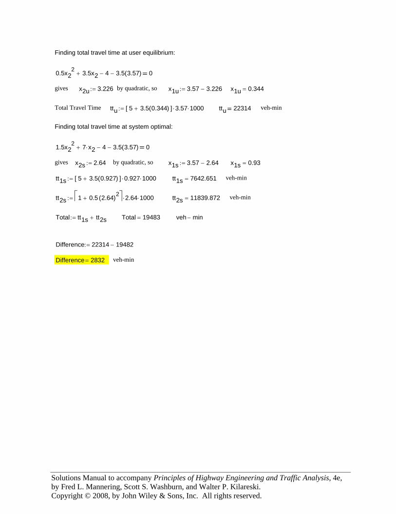
Solutions Manual to accompany Principles of Highway Engineering and Traffic Analysis, 4e, by Fred L. Mannering, Scott S. Washburn, and Walter P. Kilareski. Copyright © 2008, by John Wiley & Sons, Inc. All rights reserved.
veh-min Difference 2832=
Difference 22314 19482−:=
veh min−Total 19483=Total tt1s tt2s+:=
veh-min tt2s 11839.872=tt2s 1 0.5 2.64( )2+⎡⎣ ⎤⎦ 2.64⋅ 1000⋅:=
veh-min tt1s 7642.651=tt1s 5 3.5 0.927( )+[ ] 0.927⋅ 1000⋅:=
x1s 0.93=x1s 3.57 2.64−:=by quadratic, sox2s 2.64:=gives
1.5x22 7 x2⋅+ 4− 3.5 3.57( )− 0
Finding total travel time at system optimal:
veh-min ttu 22314ttu 5 3.5 0.344( )+[ ] 3.57⋅ 1000⋅:=Total Travel Time
x1u 0.344=x1u 3.57 3.226−:=by quadratic, sox2u 3.226:=gives
0.5x22 3.5x2+ 4− 3.5 3.57( )− 0
Finding total travel time at user equilibrium:
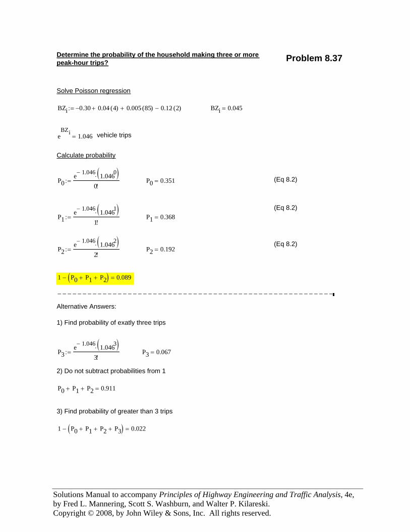
Solutions Manual to accompany Principles of Highway Engineering and Traffic Analysis, 4e, by Fred L. Mannering, Scott S. Washburn, and Walter P. Kilareski. Copyright © 2008, by John Wiley & Sons, Inc. All rights reserved.
Determine the probability of the household making three or morepeak-hour trips? Problem 8.37
Solve Poisson regression
BZi 0.30− 0.04 4( )⋅+ 0.005 85( )⋅+ 0.12 2( )⋅−:= BZi 0.045=
eBZi 1.046= vehicle trips
Calculate probability
P0e 1.046− 1.0460( )⋅
0!:= P0 0.351= (Eq 8.2)
(Eq 8.2)P1
e 1.046− 1.0461( )⋅
1!:= P1 0.368=
(Eq 8.2)P2
e 1.046− 1.0462( )⋅
2!:= P2 0.192=
1 P0 P1+ P2+( )− 0.089=
−−−−−−−−−−−−−−−−−−−−−−−−−−−−−−−−−−−−−−−−−−−−−−−−−−−−−−−
Alternative Answers:
1) Find probability of exatly three trips
P3e 1.046− 1.0463( )⋅
3!:= P3 0.067=
2) Do not subtract probabilities from 1
P0 P1+ P2+ 0.911=
3) Find probability of greater than 3 trips
1 P0 P1+ P2+ P3+( )− 0.022=
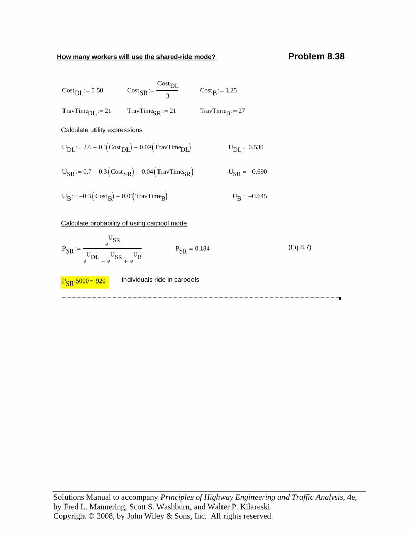
Solutions Manual to accompany Principles of Highway Engineering and Traffic Analysis, 4e, by Fred L. Mannering, Scott S. Washburn, and Walter P. Kilareski. Copyright © 2008, by John Wiley & Sons, Inc. All rights reserved.
How many workers will use the shared-ride mode? Problem 8.38
CostDL 5.50:= CostSRCostDL
3:= CostB 1.25:=
TravTimeDL 21:= TravTimeSR 21:= TravTimeB 27:=
Calculate utility expressions
UDL 2.6 0.3 CostDL( )− 0.02 TravTimeDL( )⋅−:= UDL 0.530=
USR 0.7 0.3 CostSR( )⋅− 0.04 TravTimeSR( )⋅−:= USR 0.690−=
UB 0.3− CostB( )⋅ 0.01 TravTimeB( )−:= UB 0.645−=
Calculate probability of using carpool mode
PSReUSR
eUDL e
USR+ e
UB+
:= PSR 0.184= (Eq 8.7)
PSR 5000⋅ 920= individuals ride in carpools
−−−−−−−−−−−−−−−−−−−−−−−−−−−−−−−−−−−−−−−−−−−−−−−−−−−−−−−
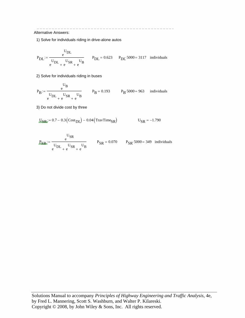
Solutions Manual to accompany Principles of Highway Engineering and Traffic Analysis, 4e, by Fred L. Mannering, Scott S. Washburn, and Walter P. Kilareski. Copyright © 2008, by John Wiley & Sons, Inc. All rights reserved.
−−−−−−−−−−−−−−−−−−−−−−−−−−−−−−−−−−−−−−−−−−−−−−Alternative Answers:
1) Solve for individuals riding in drive-alone autos
PDLeUDL
eUDL e
USR+ e
UB+
:= PDL 0.623= PDL 5000⋅ 3117= individuals
2) Solve for individuals riding in buses
PBeUB
eUDL e
USR+ e
UB+
:= PB 0.193= PB 5000⋅ 963= individuals
3) Do not divide cost by three
USR 0.7 0.3 CostDL( )⋅− 0.04 TravTimeSR( )⋅−:= USR 1.790−=
PSReUSR
eUDL e
USR+ e
UB+
:= PSR 0.070= PSR 5000⋅ 349= individuals
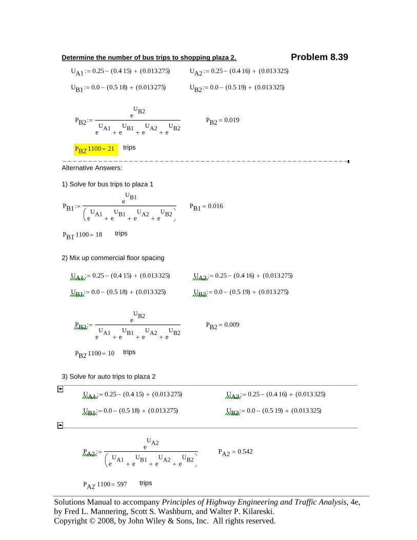
Solutions Manual to accompany Principles of Highway Engineering and Traffic Analysis, 4e, by Fred L. Mannering, Scott S. Washburn, and Walter P. Kilareski. Copyright © 2008, by John Wiley & Sons, Inc. All rights reserved.
Determine the number of bus trips to shopping plaza 2. Problem 8.39UA1 0.25 0.4 15⋅( )− 0.013 275⋅( )+:= UA2 0.25 0.4 16⋅( )− 0.013 325⋅( )+:=
UB1 0.0 0.5 18⋅( )− 0.013 275⋅( )+:= UB2 0.0 0.5 19⋅( )− 0.013 325⋅( )+:=
PB2e
UB2
eUA1 e
UB1+ e
UA2+ e
UB2+
:= PB2 0.019=
PB2 1100⋅ 21= trips
−−−−−−−−−−−−−−−−−−−−−−−−−−−−−−−−−−−−−−−−−−−−−−−−−−−−−−−−Alternative Answers:
1) Solve for bus trips to plaza 1
PB1eUB1
eUA1 e
UB1+ e
UA2+ e
UB2+
⎛⎝
⎞⎠
:= PB1 0.016=
PB1 1100⋅ 18= trips
2) Mix up commercial floor spacing
UA1 0.25 0.4 15⋅( )− 0.013 325⋅( )+:= UA2 0.25 0.4 16⋅( )− 0.013 275⋅( )+:=
UB1 0.0 0.5 18⋅( )− 0.013 325⋅( )+:= UB2 0.0 0.5 19⋅( )− 0.013 275⋅( )+:=
PB2eUB2
eUA1 e
UB1+ e
UA2+ e
UB2+
:= PB2 0.009=
PB2 1100⋅ 10= trips
3) Solve for auto trips to plaza 2
UA1 0.25 0.4 15⋅( )− 0.013 275⋅( )+:= UA2 0.25 0.4 16⋅( )− 0.013 325⋅( )+:=
UB1 0.0 0.5 18⋅( )− 0.013 275⋅( )+:= UB2 0.0 0.5 19⋅( )− 0.013 325⋅( )+:=
PA2eUA2
eUA1 e
UB1+ e
UA2+ e
UB2+
⎛⎝
⎞⎠
:= PA2 0.542=
PA2 1100⋅ 597= trips
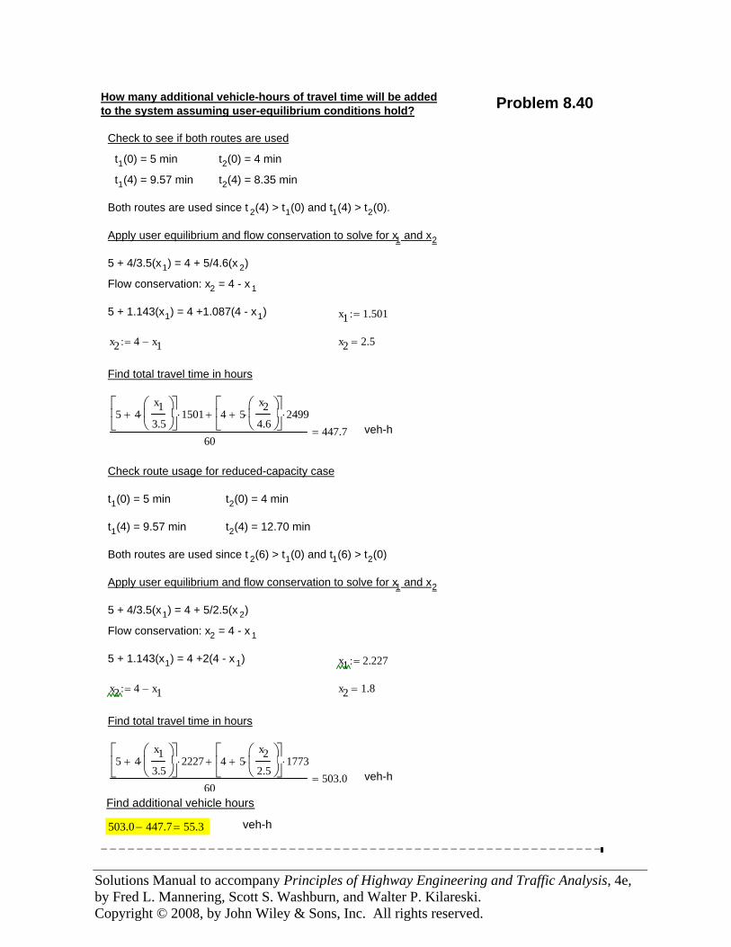
Solutions Manual to accompany Principles of Highway Engineering and Traffic Analysis, 4e, by Fred L. Mannering, Scott S. Washburn, and Walter P. Kilareski. Copyright © 2008, by John Wiley & Sons, Inc. All rights reserved.
How many additional vehicle-hours of travel time will be addedto the system assuming user-equilibrium conditions hold? Problem 8.40
Check to see if both routes are used
t1(0) = 5 min t2(0) = 4 min
t1(4) = 9.57 min t2(4) = 8.35 min
Both routes are used since t 2(4) > t1(0) and t1(4) > t2(0).
Apply user equilibrium and flow conservation to solve for x1 and x2
5 + 4/3.5(x1) = 4 + 5/4.6(x 2)
Flow conservation: x2 = 4 - x 1
5 + 1.143(x1) = 4 +1.087(4 - x1) x1 1.501:=
x2 4 x1−:= x2 2.5=
Find total travel time in hours
5 4x13.5
⎛⎜⎝
⎞⎟⎠
⋅+⎡⎢⎣
⎤⎥⎦
1501⋅ 4 5x24.6
⎛⎜⎝
⎞⎟⎠
⋅+⎡⎢⎣
⎤⎥⎦
2499⋅+
60447.7= veh-h
Check route usage for reduced-capacity case
t1(0) = 5 min t2(0) = 4 min
t1(4) = 9.57 min t2(4) = 12.70 min
Both routes are used since t 2(6) > t1(0) and t1(6) > t2(0)
Apply user equilibrium and flow conservation to solve for x1 and x2
5 + 4/3.5(x1) = 4 + 5/2.5(x 2)
Flow conservation: x2 = 4 - x 1
5 + 1.143(x1) = 4 +2(4 - x 1) x1 2.227:=
x2 4 x1−:= x2 1.8=
Find total travel time in hours
5 4x13.5
⎛⎜⎝
⎞⎟⎠
⋅+⎡⎢⎣
⎤⎥⎦
2227⋅ 4 5x22.5
⎛⎜⎝
⎞⎟⎠
⋅+⎡⎢⎣
⎤⎥⎦
1773⋅+
60503.0= veh-h
Find additional vehicle hours
503.0 447.7− 55.3= veh-h
−−−−−−−−−−−−−−−−−−−−−−−−−−−−−−−−−−−−−−−−−−−−−−−−−−−−−−−−
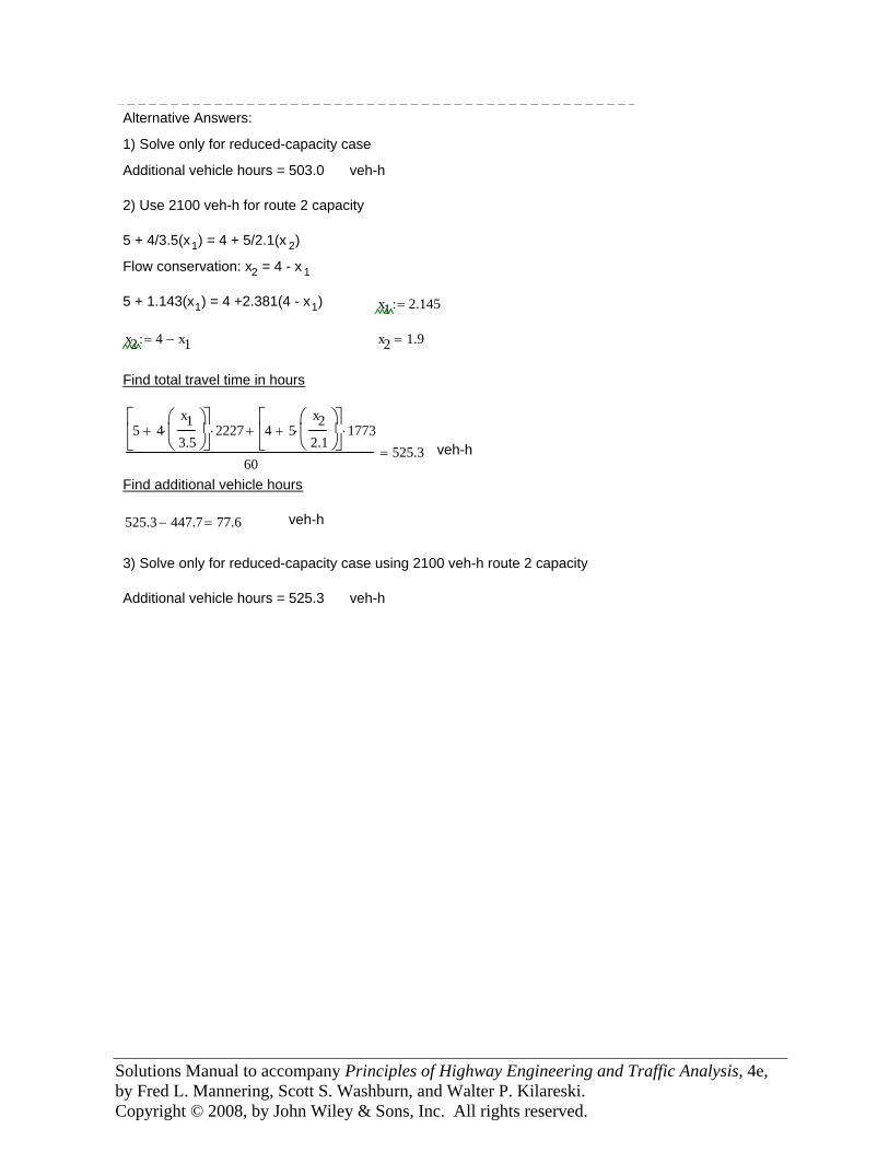
Solutions Manual to accompany Principles of Highway Engineering and Traffic Analysis, 4e, by Fred L. Mannering, Scott S. Washburn, and Walter P. Kilareski. Copyright © 2008, by John Wiley & Sons, Inc. All rights reserved.
−−−−−−−−−−−−−−−−−−−−−−−−−−−−−−−−−−−−−−−−−−−−−−−−Alternative Answers:
1) Solve only for reduced-capacity case
Additional vehicle hours = 503.0 veh-h
2) Use 2100 veh-h for route 2 capacity
5 + 4/3.5(x1) = 4 + 5/2.1(x 2)
Flow conservation: x2 = 4 - x 1
5 + 1.143(x1) = 4 +2.381(4 - x1) x1 2.145:=
x2 4 x1−:= x2 1.9=
Find total travel time in hours
5 4x13.5
⎛⎜⎝
⎞⎟⎠
⋅+⎡⎢⎣
⎤⎥⎦
2227⋅ 4 5x22.1
⎛⎜⎝
⎞⎟⎠
⋅+⎡⎢⎣
⎤⎥⎦
1773⋅+
60525.3= veh-h
Find additional vehicle hours
525.3 447.7− 77.6= veh-h
3) Solve only for reduced-capacity case using 2100 veh-h route 2 capacity
Additional vehicle hours = 525.3 veh-h
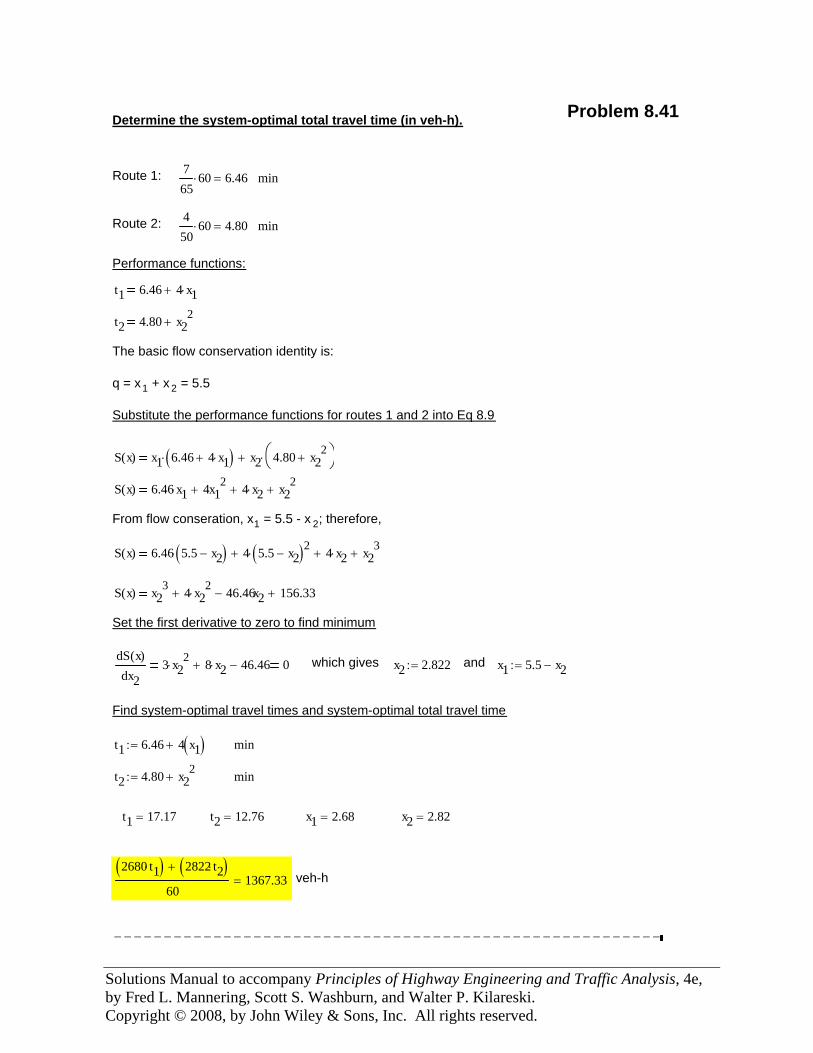
Solutions Manual to accompany Principles of Highway Engineering and Traffic Analysis, 4e, by Fred L. Mannering, Scott S. Washburn, and Walter P. Kilareski. Copyright © 2008, by John Wiley & Sons, Inc. All rights reserved.
Problem 8.41Determine the system-optimal total travel time (in veh-h).
Route 1: 765
60⋅ 6.46= min
Route 2: 450
60⋅ 4.80= min
Performance functions:
t1 6.46 4 x1⋅+
t2 4.80 x22
+
The basic flow conservation identity is:
q = x1 + x 2 = 5.5
Substitute the performance functions for routes 1 and 2 into Eq 8.9
S x( ) x1 6.46 4 x1⋅+( )⋅ x2 4.80 x22
+⎛⎝
⎞⎠⋅+
S x( ) 6.46 x1⋅ 4x12
+ 4 x2⋅+ x22
+
From flow conseration, x1 = 5.5 - x 2; therefore,
S x( ) 6.46 5.5 x2−( )⋅ 4 5.5 x2−( )2⋅+ 4 x2⋅+ x23
+
S x( ) x23 4 x2
2⋅+ 46.46x2− 156.33+
Set the first derivative to zero to find minimum
dS x( )dx2
3 x22
⋅ 8 x2⋅+ 46.46− 0 which gives x2 2.822:= and x1 5.5 x2−:=
Find system-optimal travel times and system-optimal total travel time
t1 6.46 4 x1( )+:= min
t2 4.80 x22
+:= min
t1 17.17= t2 12.76= x1 2.68= x2 2.82=
2680 t1⋅( ) 2822 t2⋅( )+
601367.33= veh-h
−−−−−−−−−−−−−−−−−−−−−−−−−−−−−−−−−−−−−−−−−−−−−−−−−−−−−−−
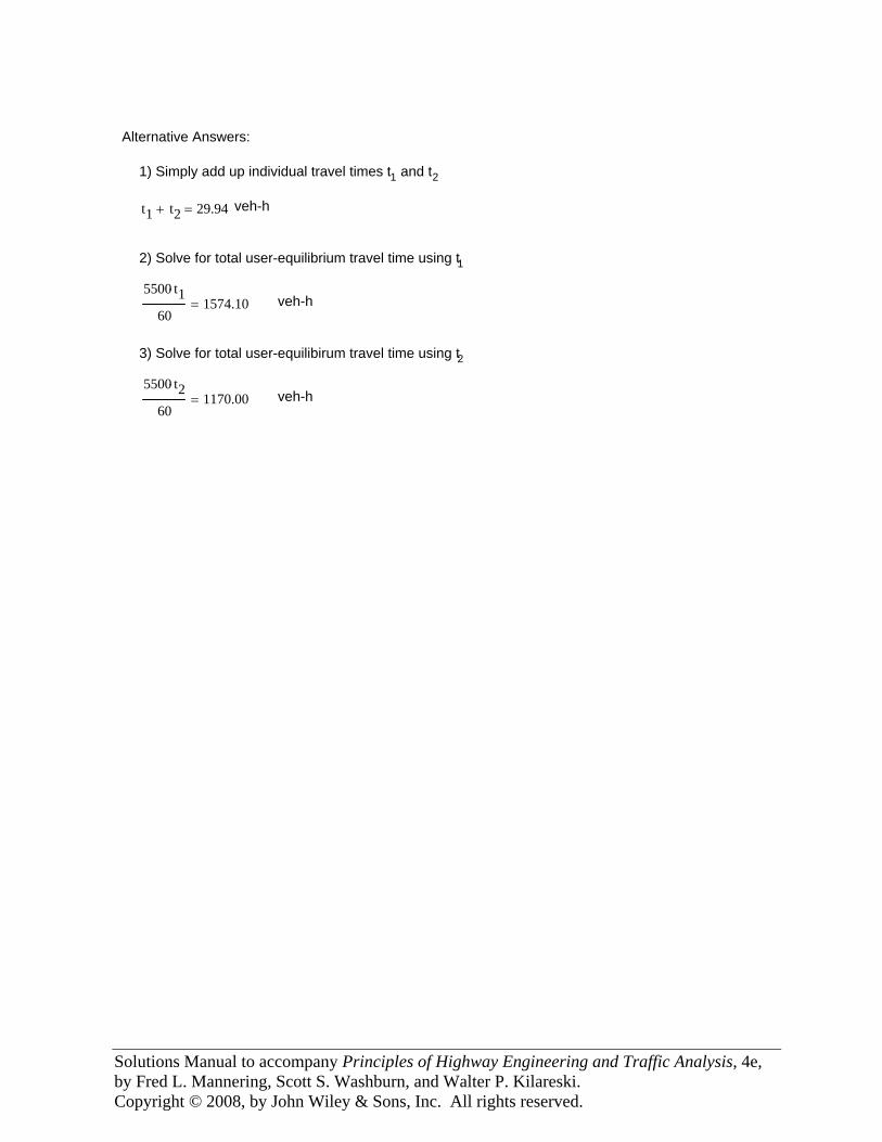
Solutions Manual to accompany Principles of Highway Engineering and Traffic Analysis, 4e, by Fred L. Mannering, Scott S. Washburn, and Walter P. Kilareski. Copyright © 2008, by John Wiley & Sons, Inc. All rights reserved.
−−−−−−−−−−−−−−−−−−−−−−−−−−−−−−−−−Alternative Answers:
1) Simply add up individual travel times t1 and t2
t1 t2+ 29.94= veh-h
2) Solve for total user-equilibrium travel time using t1
5500 t1⋅
601574.10= veh-h
3) Solve for total user-equilibirum travel time using t2
5500 t2⋅
601170.00= veh-h
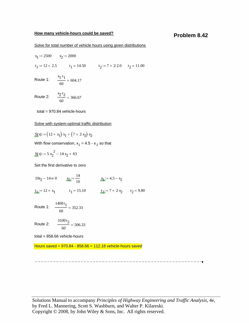
Solutions Manual to accompany Principles of Highway Engineering and Traffic Analysis, 4e, by Fred L. Mannering, Scott S. Washburn, and Walter P. Kilareski. Copyright © 2008, by John Wiley & Sons, Inc. All rights reserved.
How many vehicle-hours could be saved? Problem 8.42Solve for total number of vehicle hours using given distributions
x1 2500:= x2 2000:=
t1 12 2.5+:= t1 14.50= t2 7 2 2.0⋅+:= t2 11.00=
Route 1:x1 t1⋅
60604.17=
Route 2:x2 t2⋅
60366.67=
total = 970.84 vehicle-hours
Solve with system-optimal traffic distribution
S x( ) 12 x1+( ) x1⋅ 7 2 x2⋅+( ) x2⋅+:=
With flow conservation, x1 = 4.5 - x 2 so that
S x( ) 5 x22
⋅ 14 x2⋅− 63+:=
Set the first derivative to zero
10x2 14− 0 x21410
:= x1 4.5 x2−:=
t1 12 x1+:= t1 15.10= t2 7 2 x2⋅+:= t2 9.80=
Route 1:1400 t1⋅
60352.33=
Route 2:3100 t2⋅
60506.33=
total = 858.66 vehicle-hours
Hours saved = 970.84 - 858.66 = 112.18 vehicle-hours saved
−−−−−−−−−−−−−−−−−−−−−−−−−−−−−−−−−−−−−−−−−−−−−−−−−−−−−−−
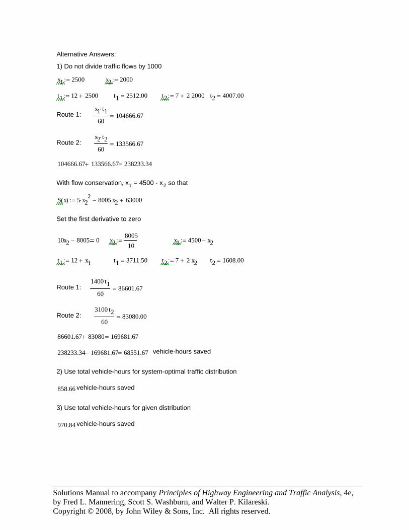
Solutions Manual to accompany Principles of Highway Engineering and Traffic Analysis, 4e, by Fred L. Mannering, Scott S. Washburn, and Walter P. Kilareski. Copyright © 2008, by John Wiley & Sons, Inc. All rights reserved.
Alternative Answers:
1) Do not divide traffic flows by 1000
x1 2500:= x2 2000:=
t1 12 2500+:= t1 2512.00= t2 7 2 2000⋅+:= t2 4007.00=
Route 1:x1 t1⋅
60104666.67=
Route 2:x2 t2⋅
60133566.67=
104666.67 133566.67+ 238233.34=
With flow conservation, x1 = 4500 - x2 so that
S x( ) 5 x22
⋅ 8005 x2⋅− 63000+:=
Set the first derivative to zero
10x2 8005− 0 x2800510
:= x1 4500 x2−:=
t1 12 x1+:= t1 3711.50= t2 7 2 x2⋅+:= t2 1608.00=
Route 1:1400 t1⋅
6086601.67=
Route 2:3100 t2⋅
6083080.00=
86601.67 83080+ 169681.67=
238233.34 169681.67− 68551.67= vehicle-hours saved
2) Use total vehicle-hours for system-optimal traffic distribution
858.66 vehicle-hours saved
3) Use total vehicle-hours for given distribution
970.84 vehicle-hours saved