Principes de choix de portefeuille - Freeboucher.univ.free.fr/publis/cours/2015/CB_CPCh4_2015.pdf · ® 2009 Pearson Education France transparents traduits par Vincent Dropsy Principes

® 2009 Pearson Education France

transparents traduits par Vincent Dropsy

Principes de choix

de portefeuille7e édition

Christophe Boucher

[email protected]

1


transparents traduits par Vincent Dropsy

Chapitre 47e édition

La théorie Moyenne-Variance du choix de portefeuille

2


transparents traduits par Vincent Dropsy Principes de choix de portefeuille –Christophe BOUCHER – 2015/2016

Part 4. Mean-Variance Portfolio Theory

3

4.1 Measuring Risk and Return

4.2 Asset Allocation with 2 Risky Assets

4.3 Introducing a Risk Free Asset and the Tobin’s Separation Theorem

4.4 Asset Allocation with N risky Assets

4.5 Portfolio Diversification



Preamble:

Mean/Variance Analysis Assumptions

4



Mean-variance is simpler

5

• Early researchers in finance, such as Markowitz and Sharpe, used just the mean and the variance of the return rate of an asset to describe it.

• Characterizing the prospects of a gamble with its mean and variance is often easier than using an NM utility function, so it is popular.

• But is it compatible with VNM theory?

• The answer is yes … approximately … under some conditions.



Mean-variance assumptions

6

• Investors maximise expected utility of end-of-perio d wealth

• Can be shown that above implies maximise a function of expected portfolio returns and portfolio variance p roviding

- Either utility is quadratic, or

- Portfolio returns are normally distributed (and utility is concave),

- Consider only small risks (then approximately true)



Mean-variance: quadratic utility

7

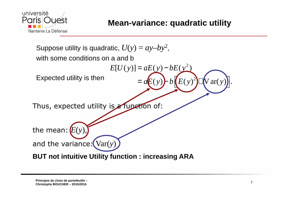
Suppose utility is quadratic, U(y) = ay–by2,

with some conditions on a and b

Expected utility is then

2

2

[ ( )] ( ) ( )

( ) ( ) V ar( ) .

E U y aE y bE y

aE y b E y y

= −

= − +

Thus, expected utility is a function of:

the mean: E(y),

and the variance: Var(y)

BUT not intuitive Utility function : increasing ARA



Mean-variance: joint normals

8

• Suppose all lotteries in the domain have normally distributed prized. (They need not be independent of each other).

• Any combination of such lotteries will also be normally distributed.

• The normal distribution is completely described by its first two moments.

• Therefore, the distribution of any combination of lotteries is also completely described by just the mean and the variance.

• As a result, expected utility can be expressed as a function of just these two numbers as well.



Mean-variance: small risks

9

• The most relevant justification for mean-variance is probably the case of small risks.

• If we consider only small risks, we may use a second order Taylor approximation of the NM utility function.

• A second order Taylor approximation of a concave function is a quadratic function with a negative coefficient on the quadratic term.

• In other words, any risk-averse NM utility function can locally be approximated with a quadratic function.

• But the expectation of a quadratic utility function can be evaluated with the mean and variance. Thus, to evaluate small risks, mean and variance are enough.




10

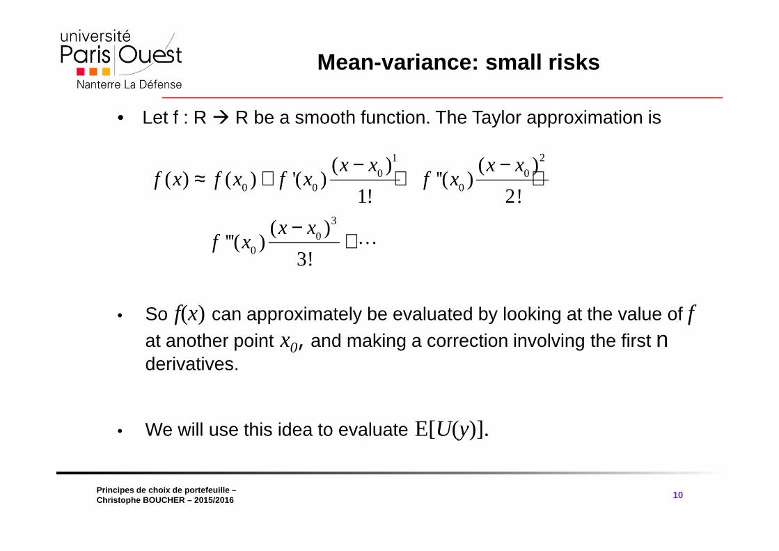
• Let f : R R be a smooth function. The Taylor approximation is

• So f(x) can approximately be evaluated by looking at the value of fat another point x0, and making a correction involving the first nderivatives.

• We will use this idea to evaluate E[U(y)].

1 2

0 00 0 0

3

00

( ) ( )( ) ( ) '( ) ''( )

1! 2!

( )'''( )

3!

x x x xf x f x f x f x

x xf x

− −≈ + + +

−+⋯




11

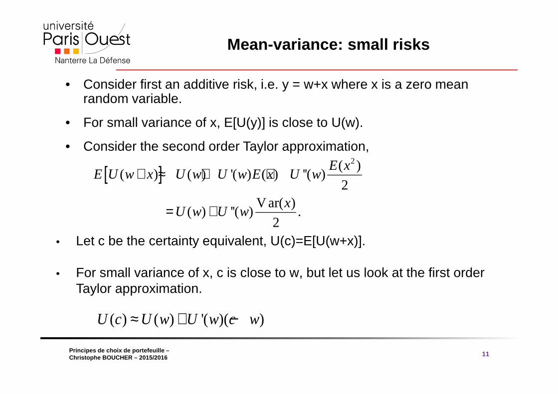
• Consider first an additive risk, i.e. y = w+x where x is a zero mean random variable.

• For small variance of x, E[U(y)] is close to U(w).

• Consider the second order Taylor approximation,

• Let c be the certainty equivalent, U(c)=E[U(w+x)].

• For small variance of x, c is close to w, but let us look at the first order Taylor approximation.

[ ]2( )

( ) ( ) '( ) ( ) ''( )2

Var( )( ) ''( ) .

2

E xE U w x U w U w E x U w

xU w U w

+ ≈ + +

= +

( ) ( ) '( )( )U c U w U w c w≈ + −




12

• Since E[U(w+x)] = U(c), this simplifies to

• w – c is the risk premium.

• The risk premium is approximately a linear function of the variance of the additive risk, with the slope of the effect equal to half the coefficient of absolute risk.

V ar( )( )

2

xw c A w− ≈



Example: Simple mean-variance utility function

13

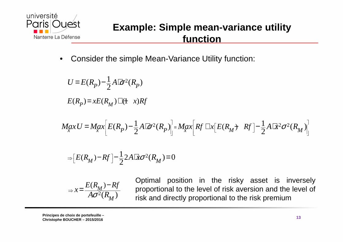
• Consider the simple Mean-Variance Utility function:

21( ) ( )2P PU E R A Rσ= − ⋅

2 2 2)(1 1( ) ( ) ( )2 2Mx x xP P MRf x E R RfMaxU Max E R A R Max A x Rσ σ

=

+ −= − ⋅ − ⋅

( ) ( ) (1 )P ME R xE R x Rf= + −

2)( 21 ( ) 02M ME R Rf A x Rσ ⇒

− − ⋅ =

2

)(( )

M

M

E R Rfx

A Rσ⇒−=

Optimal position in the risky asset is inverselyproportional to the level of risk aversion and the level ofrisk and directly proportional to the risk premium



4.1 Measuring Risk and Return

14



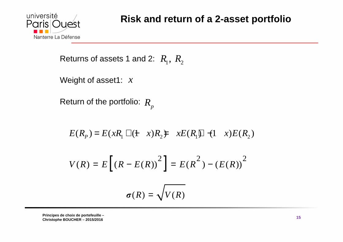
Returns of assets 1 and 2:

Weight of asset1:

Return of the portfolio:

Risk and return of a 2-asset portfolio

15

1 2, R R

x

pR

1 2 1 2( ) ( (1 ) ) ( ) (1 ) ( )PE R E xR x R xE R x E R= + − = + −

[ ]2 2 2( ) ( ( )) ( ) ( ( ))V R E R E R E R E R= − = −

( ) ( )R V Rσ =



Risk and return of a 2-asset portfolio

16

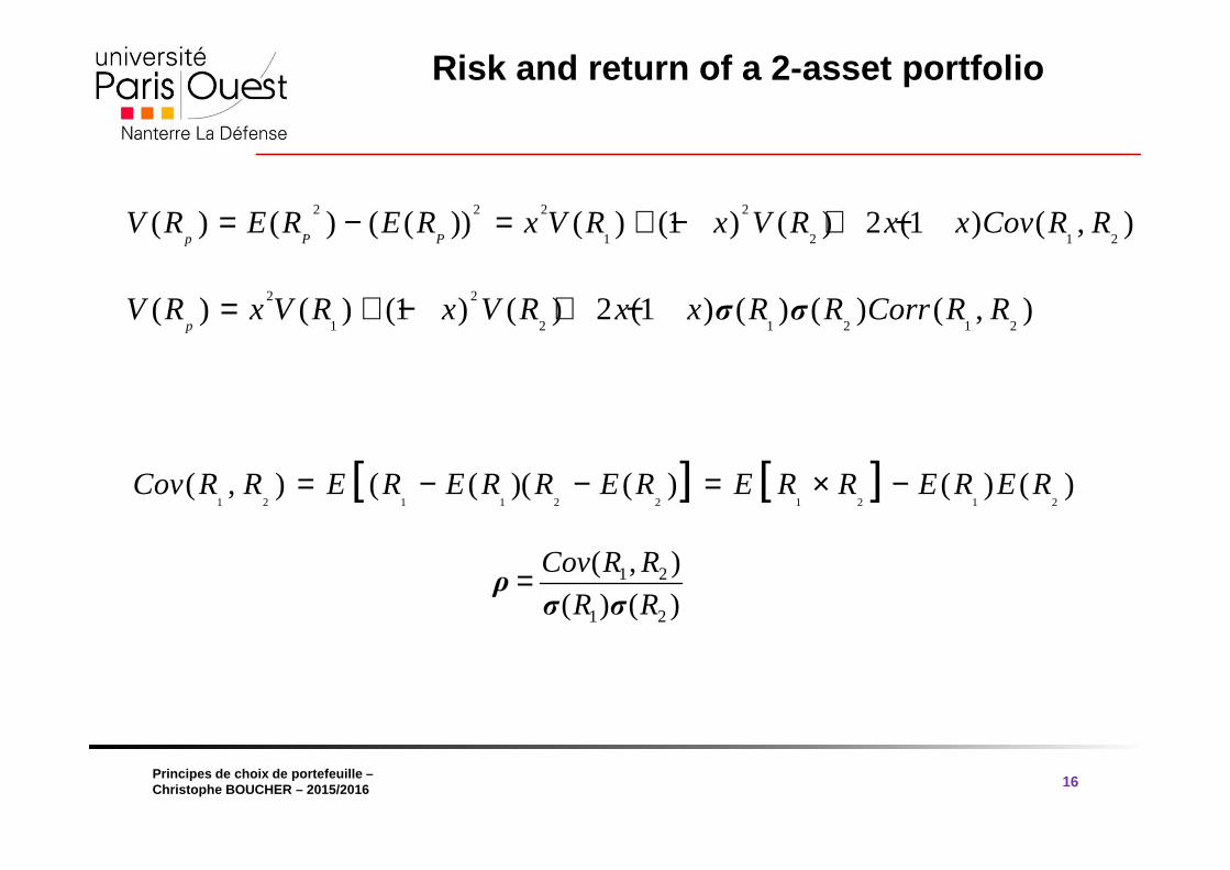
2 2 2 2

1 2 1 2( ) ( ) ( ( )) ( ) (1 ) ( ) 2 (1 ) ( , )

p P PV R E R E R x V R x V R x x Cov R R= − = + − + −

2 2

1 2 1 2 1 2( ) ( ) (1 ) ( ) 2 (1 ) ( ) ( ) ( , )

pV R x V R x V R x x R R Corr R Rσ σ= + − + −

[ ] [ ]1 2 1 1 2 2 1 2 1 2

( , ) ( ( )( ( ) ( ) ( )Cov R R E R E R R E R E R R E R E R= − − = × −

1 2

1 2

( , )

( ) ( )

Cov R R

R R=ρσ σ



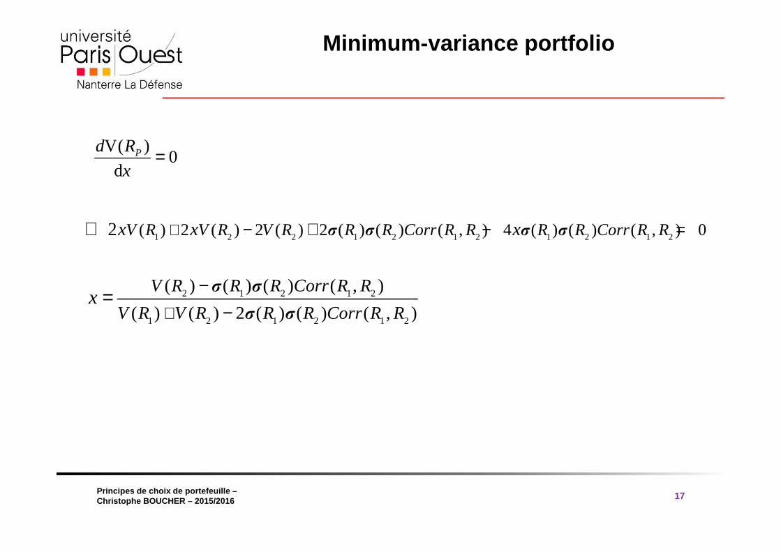
Minimum -variance portfolio

17

V( )0

dPd R

x=

1 2 2 1 2 1 2 1 2 1 2( ) 2 ( ) 2 ( ) 2 ( ) ( ) ( , ) 4 ( ) ( ) ( , ) 02 V R V R V R R R Corr R R R R Corr R Rx x xσ σ σ σ+ − + − =⇔

2 1 2 1 2

1 2 1 2 1 2

( ) ( ) ( ) ( , )

( ) ( ) 2 ( ) ( ) ( , )

V R R R Corr R R

V R V R R R Corr R Rx

σ σ

σ σ+

−−

=



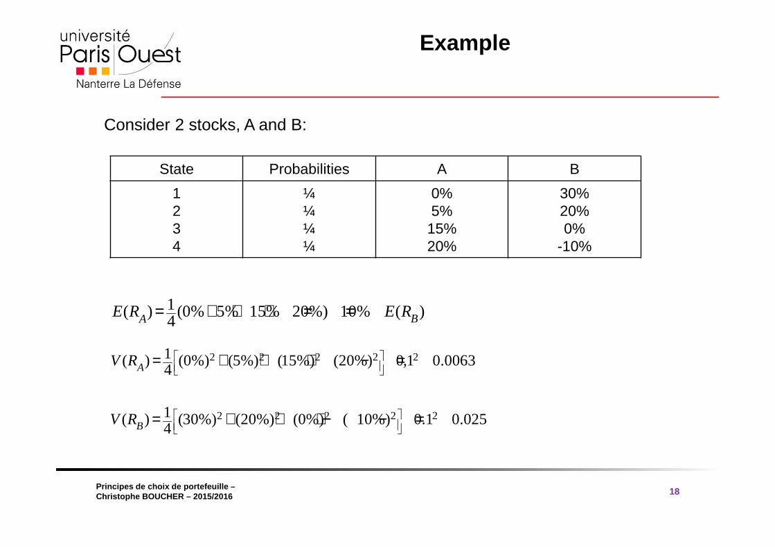
Example

18

Consider 2 stocks, A and B:

State Probabilities A B

1234

¼¼¼¼

0%5%

15%20%

30%20%0%

-10%

1( ) (0% 5% 15% 20%) 10% ( )4 BAE R E R= + + + = =

2 2 2 2 21( ) (0%) (5%) (15%) (20%) 0,1 0.00634AV R

= + + + − =

2 2 2 2 21( ) (30%) (20%) (0%) ( 10%) 0.1 0.0254BV R

= + + + − − =



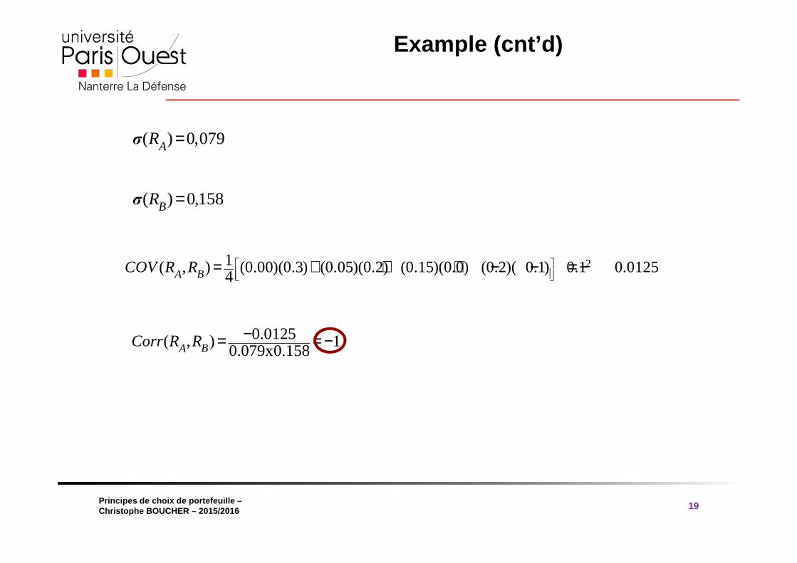
Example (cnt’d)

19

( ) 0,079AR =σ

( ) 0,158BR =σ

21( , ) (0.00)(0.3) (0.05)(0.2) (0.15)(0.0) (0.2)( 0.1) 0.1 0.01254BACOV R R

= + + + − − = −

0.0125( , ) 10.079x0.158BACorr R R −= = −



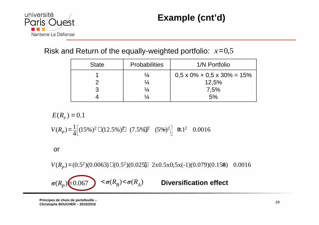
Example (cnt’d)

20

Risk and Return of the equally-weighted portfolio: 0,5x=

State Probabilities 1/N Portfolio

1234

¼¼¼¼

0,5 x 0% + 0,5 x 30% = 15%12,5%7,5%5%

( ) 0.1PE R =

2 2 2 2 21( ) (15%) (12.5%) (7.5%) (5%) 0.1 0.00164PV R

= + + + − =

or

2 2( ) (0.5 )(0.0063) (0.5 )(0.025) 2x0.5x0;5x(-1)(0.079)(0.158) 0.0016PV R = + + =

( ) 0.067PR =σ ( ) ( )B AR R< <σ σ Diversification effect



Example (cnt’d)

21

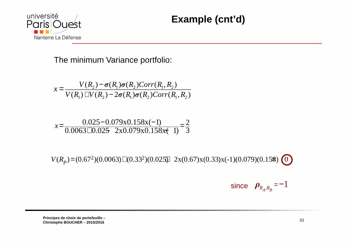
The minimum Variance portfolio:

2 1 2 1 2

1 2 1 2 1 2

( ) ( ) ( ) ( , )( ) ( ) 2 ( ) ( ) ( , )

V R R R Corr R RV R V R R R Corr R R

x+

−−

= σ σ

σ σ

0.025 0.079x0.158x( 1) 230.0063 0.025 2x0.079x0.158x( 1)

x − −= =+ − −

2 2( ) (0.67 )(0.0063) (0.33 )(0.025) 2x(0.67)x(0.33)x(-1)(0.079)(0.158) 0PV R = + + =

since , 1BAR R =−ρ



4.2 Asset Allocation with 2 Risky Assets

22



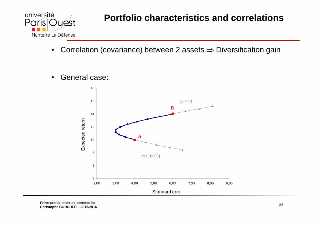
Portfolio characteristics and correlations

23

• Correlation (covariance) between 2 assets ⇒ Diversification gain

• General case:

4

6

8

10

12

14

16

18

2,00 3,00 4,00 5,00 6,00 7,00 8,00 9,00

A

B

(x>100%)

(x < 0)

4

6

8

10

12

14

16

18

2,00 3,00 4,00 5,00 6,00 7,00 8,00 9,004

6

8

10

12

14

16

18

2,00 3,00 4,00 5,00 6,00 7,00 8,00 9,00

A

B

(x>100%)

(x < 0)

Exp

ecte

d re

turn

Standard error



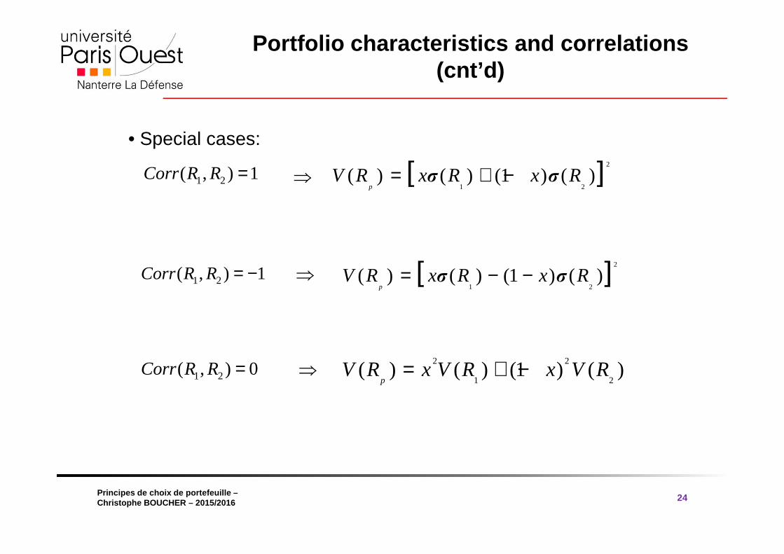
Portfolio characteristics and correlations (cnt’d)

24

• Special cases:

1 2( , ) 1Corr R R =

1 2( , ) 1Corr R R = −

1 2( , ) 0Corr R R =

[ ]2

1 2( ) ( ) (1 ) ( )

pV R x R x R= + −σ σ⇒

[ ]2

1 2( ) ( ) (1 ) ( )

pV R x R x Rσ σ= − −⇒

2 2

1 2( ) ( ) (1 ) ( )

pV R x V R x V R= + −⇒



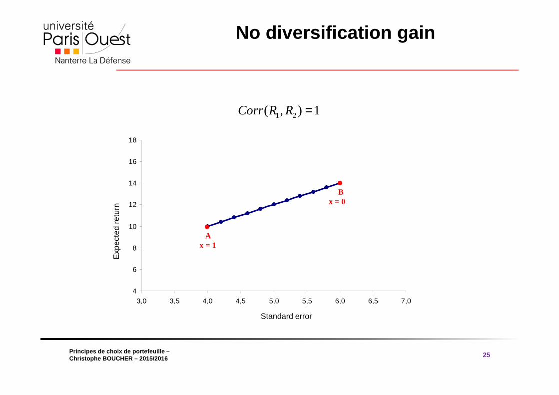
No diversification gain

25

1 2( , ) 1Corr R R =

4

6

8

10

12

14

16

18

3,0 3,5 4,0 4,5 5,0 5,5 6,0 6,5 7,0

Ren

dem

ent e

spér

é du

por

tefe

uille

(%

)

A

B

x = 1

x = 0

Exp

ecte

d re

turn

Standard error



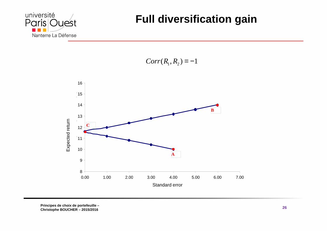
Full diversification gain

26

1 2( , ) 1Corr R R = −E

xpec

ted

retu

rn

Standard error

8

9

10

11

12

13

14

15

16

0,00 1,00 2,00 3,00 4,00 5,00 6,00 7,00Ecart type du portefeuille (%)

Ren

dem

ent e

spér

é du

por

tefe

uille

(%

)

A

B

C



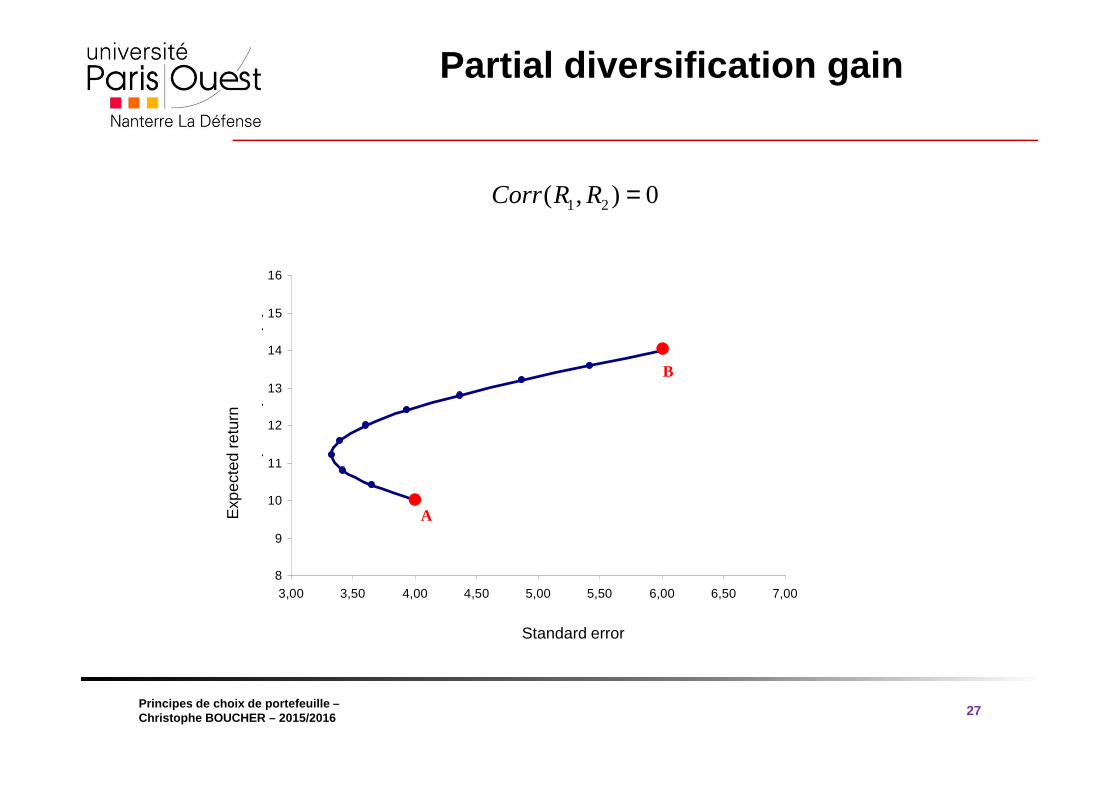
Partial diversification gain

27

1 2( , ) 0Corr R R =E

xpec

ted

retu

rn

Standard error

8

9

10

11

12

13

14

15

16

3,00 3,50 4,00 4,50 5,00 5,50 6,00 6,50 7,00

Ren

dem

ent e

spér

é du

por

tefe

uille

(%

)

A

B



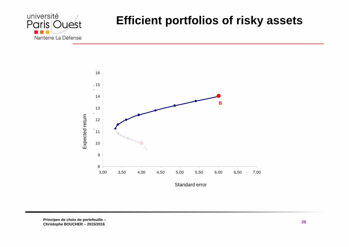
Efficient portfolios of risky assets

28

Exp

ecte

d re

turn

Standard error

8

9

10

11

12

13

14

15

16

3,00 3,50 4,00 4,50 5,00 5,50 6,00 6,50 7,00

Ren

dem

ent e

spér

é du

por

tefe

uille

(%

)

A

B



4.3 Introducing a Risk Free Asset and the Tobin’s Separation Theorem

29



Introducing borrowing and lending:Risk free asset

30

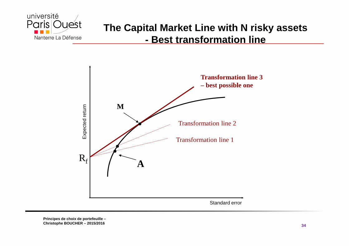
• You are now allowed to borrow and lend at the risk free rate Rf while still investing in any SINGLE ‘risky bundle’ on the efficient frontier.

• For each SINGLE risky bundle, this gives a new set of risk return combination known as the ‘transformation line’.

• The risk-return combination is a straight line (for each single risky bundle) - transformation line.

• You can be anywhere you like on this line.



The risk free asset

31

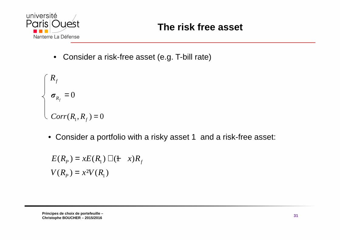
• Consider a risk-free asset (e.g. T-bill rate)

fR

0fRσ =

1( , ) 0fCorr R R =

• Consider a portfolio with a risky asset 1 and a risk-free asset:

1

1

( ) ( ) (1 )

( ) ² ( )P f

P

E R xE R x R

V R x V R

= + −

=



The Capital Market Line

32

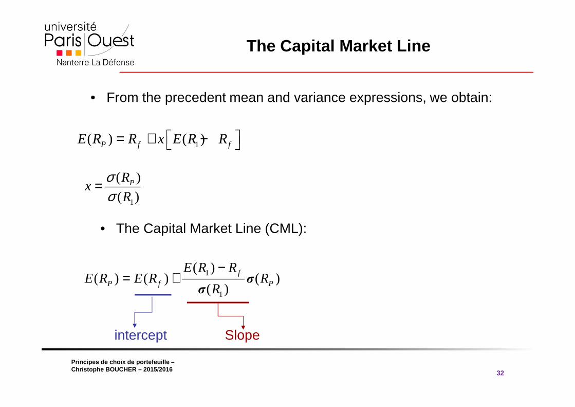
• From the precedent mean and variance expressions, we obtain:

1( ) ( )P f fE R R x E R R = + −

1

( )

( )PR

xR

σσ

=

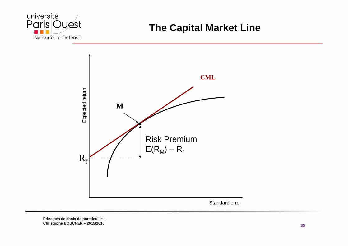
• The Capital Market Line (CML):

1

1

( )( ) ( ) ( )

( )f

P f P

E R RE R E R R

R

−= + σ

σ

Slopeintercept



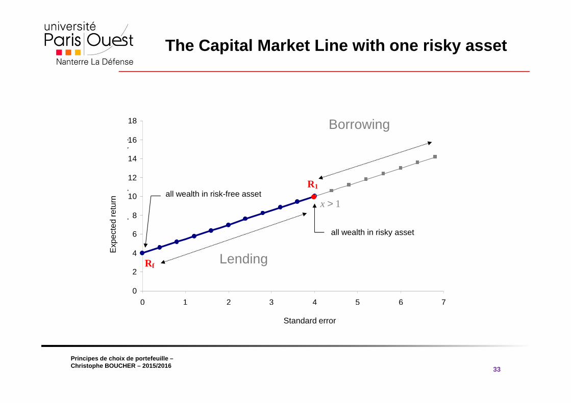
The Capital Market Line with one risky asset

33

0

2

4

6

8

10

12

14

16

18

0 1 2 3 4 5 6 7

Ren

dem

ent e

spér

é du

por

tefe

uille

(%

)

R1

Rf

x > 1

all wealth in risky asset

Exp

ecte

d re

turn

Standard error

all wealth in risk-free asset

Lending

Borrowing



The Capital Market Line with N risky assets- Best transformation line

34

Exp

ecte

d re

turn

Standard error

Transformation line 1

Transformation line 2

Transformation line 3 – best possible one

Rf A

M



The Capital Market Line

35

Exp

ecte

d re

turn

Standard error

CML

Rf

M

Risk PremiumE(RM) – Rf



The CML and the separation theorem

36

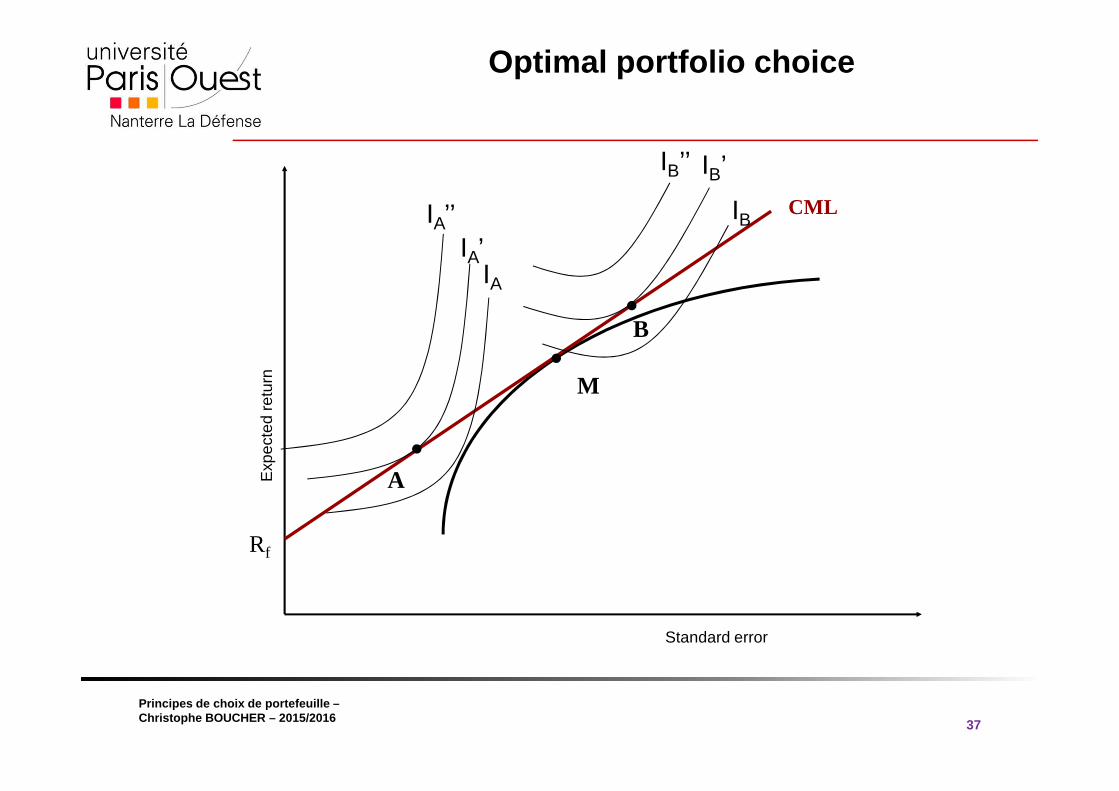
• The CML dominates all other possible portfolios

• An agent invests along the CML (where ? ⇒ risk preferences)

• James Tobin’s separation theorem:

- Invest in a risky portfolio (optimal combination of risky securities)

- Borrow-lend at the risk-free rate

• Depending on your attitude toward risk: how much lend or borrow



Optimal portfolio choice

37

Exp

ecte

d re

turn

CML

Rf

M

Standard error

A

B

IA’IA’’ IB

IA

IB’’ IB’



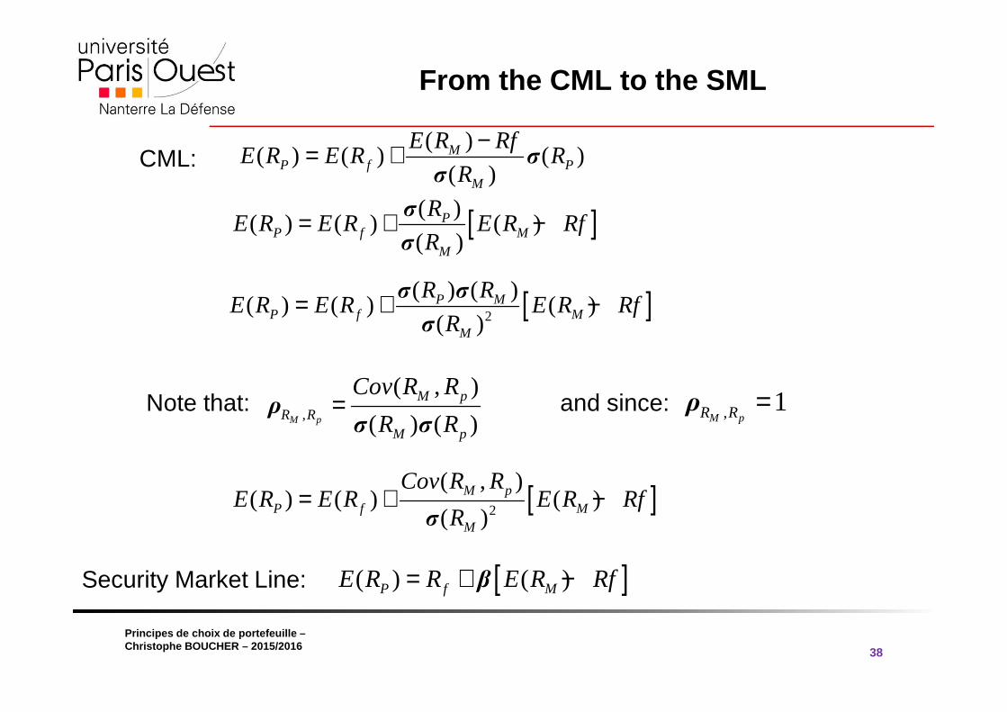
From the CML to the SML

38

( )( ) ( ) ( )

( )M

P f PM

E R RfE R E R R

R

−= + σσ

CML:

[ ]( )( ) ( ) ( )

( )P

P f MM

RE R E R E R Rf

R= + −σ

σ

Note that:,

( , )

( ) ( )M p

M pR R

M p

Cov R R

R R=ρσ σ

and since: , 1M pR R =ρ

[ ]2

( ) ( )( ) ( ) ( )

( )P M

P f MM

R RE R E R E R Rf

R= + −σ σ

σ

[ ]2

( , )( ) ( ) ( )

( )M p

P f MM

Cov R RE R E R E R Rf

R= + −

σ

Security Market Line: [ ]( ) ( )P f ME R R E R Rf= + −β



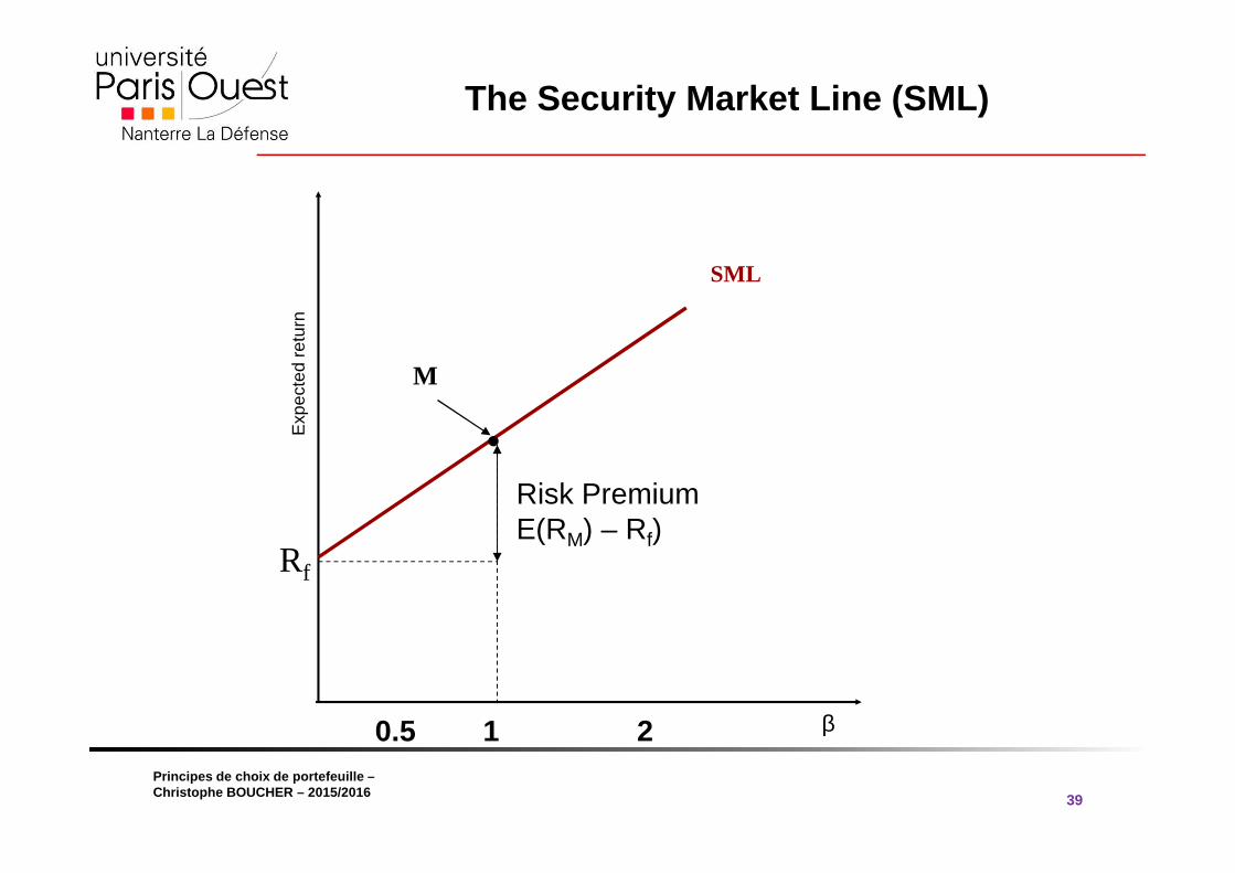
The Security Market Line (SML)

39

Exp

ecte

d re

turn

SML

Rf

M

β10.5 2

Risk PremiumE(RM) – Rf)



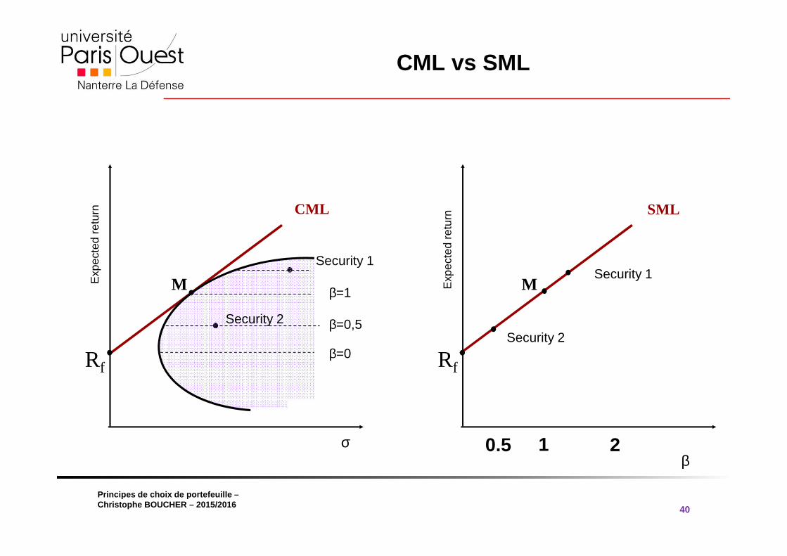
CML vs SML

40

βE

xpec

ted

retu

rn SML

Rf

M

10.5 2

Security 1

Security 2

σ

Exp

ecte

d re

turn CML

Rf

M

Security 2

Security 1

β=0

β=0,5

β=1



CML vs SML

41

• The CML: combination the market portfolio and the riskless asset

• Portfolios on the CML are efficient portfolios

• Any portfolio on the CML has a correlation of 1 with the market portfolio

• CML is applicable only to an investor’s efficient portfolio

• SML is applicable to any security, asset or portfolio (CAPM World)

• In the CML, risk is measured by σ

• In the SML, risk is measured by β



4.4 Asset Allocation with N risky Assets

42



Efficient portfolios

43

• Efficient portfolios are those that maximize the ex pected return for a given level of expected risk

• or minimize the risk for a given level of expected return

• Two kinds of efficient portfolios:

- only risky assets

- both risky assets and a riskless-asset (separation theorem)

• Suppose stable expected-returns and VCV matrix



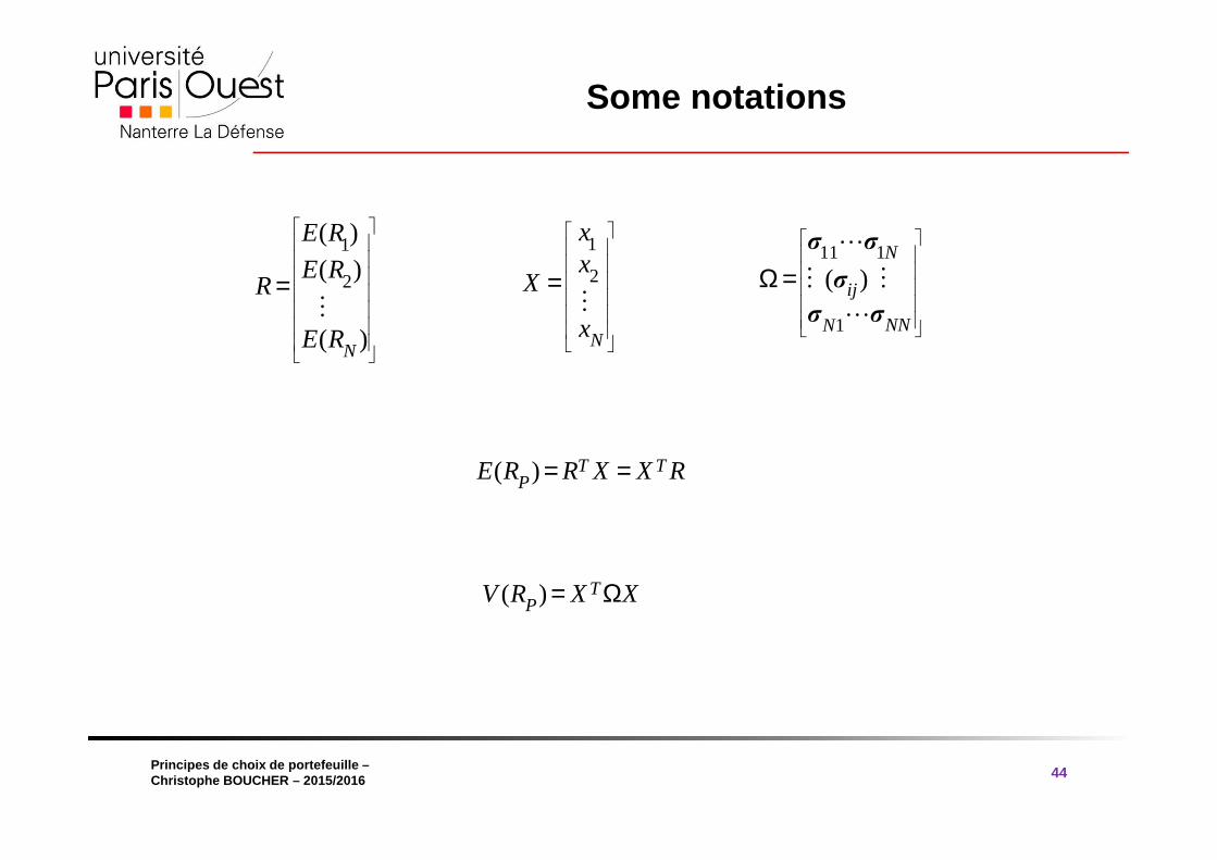
Some notations

44

1

2

( )

( )

( )N

E R

E RR

E R

=⋮

1

2

N

xx

X

x

=⋮

11 1

1

( )N

ij

NNN

Ω =⋯

⋮ ⋮

⋯

σ σ

σ

σ σ

( ) T TPE R R X X R= =

( ) TPV R X X= Ω



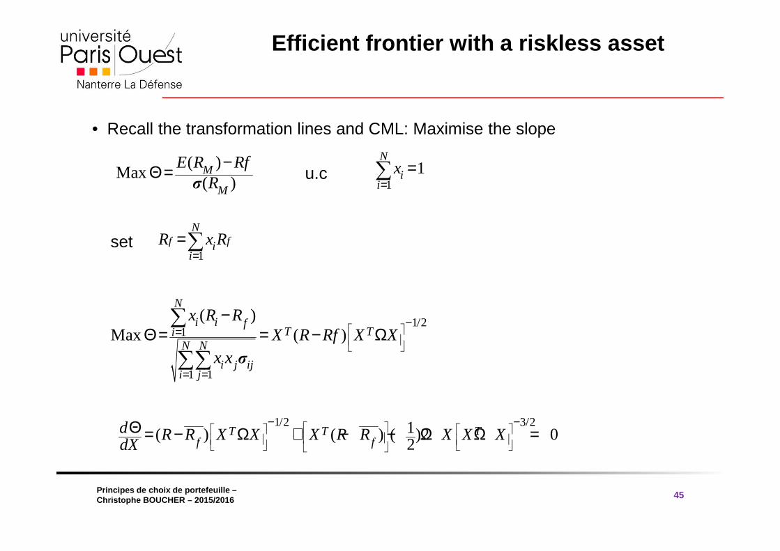
Efficient frontier with a riskless asset

45

( )Max

( )M

M

E R RfR

−Θ =σ

• Recall the transformation lines and CML: Maximise the slope

11

N

ii

x=

=∑u.c

1f f

N

ii

R x R=

=∑set

1/21

1 1

( )Max ( )

N

i i fT Ti

N N

i j iji j

x R RX R Rf X X

x x

−=

= =

−Θ = = − Ω

∑

∑∑ σ

1/2 3/21( ) ( ) ( )2 02

T T Tf f

d R R X X X R R X X XdX

− −Θ = − Ω + − − Ω Ω =



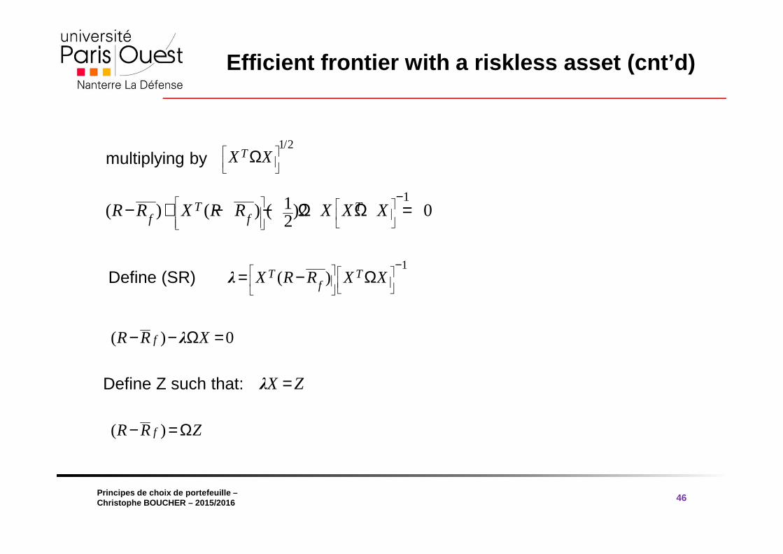
Efficient frontier with a riskless asset (cnt’d)

46

multiplying by1/2

TX X

Ω

11( ) ( ) ( )2 02

T Tf fR R X R R X X X

−− + − − Ω Ω =

1( )T T

fX R R X X

−= − ΩλDefine (SR)

( ) 0fR R X− − Ω =λ

X Z=λ

( )fR R Z− = Ω

Define Z such that:



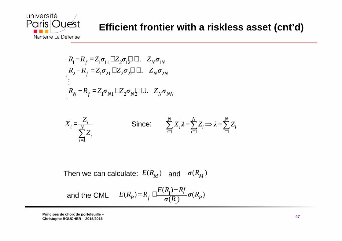
Efficient frontier with a riskless asset (cnt’d)

47

1 1 11 2 12 1

2 1 21 2 22 2

1 1 2 2

...

...

...

N Nf

N Nf

N N NNN Nf

R R Z Z Z

R R Z Z Z

R R Z Z Z

− = + + +− = + + +

− = + + +⋮

σ σ σ

σ σ σ

σ σ σ

1

ii N

ii

ZX

Z=

=∑

Since: 1 1 1

N N N

i i ii i i

X Z Z= = =

= ⇒ =∑ ∑ ∑λ λ

Then we can calculate: ( )ME R ( )MRσand

1

1

( )( ) ( )

( )P Pf

E R RfE R R R

R−= + σ

σand the CML



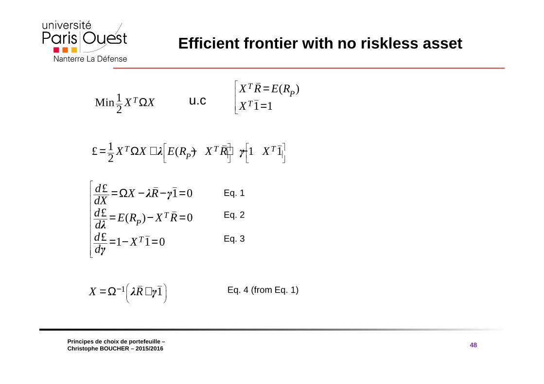
Efficient frontier with no riskless asset

48

1Min2

TX XΩ( )

1 1

TP

T

X R E R

X

==u.c

1£ ( ) 1 12

T T TPX X E R X R X

= Ω + − + −λ γ

£ 1 0

£ ( ) 0

£ 1 1 0

TP

T

d X RdXd E R X Rdd Xd

=Ω − − =

= − =

= − =

λ γ

λ

γ

1 1X R

−= Ω +λ γ

Eq. 1

Eq. 2

Eq. 3

Eq. 4 (from Eq. 1)



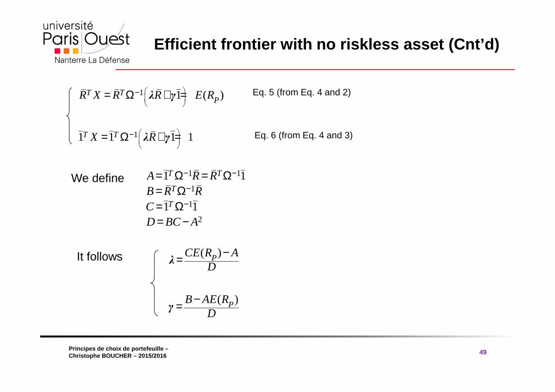
Efficient frontier with no riskless asset (Cnt’d)

49

1 1 ( )T TPR X R R E R

−= Ω + =λ γ

11 1 1 1T TX R

−= Ω + =λ γ

1 1

1

1

2

1 1

1 1

T T

T

T

A R RB R RCD BC A

− −

−

−

= Ω = Ω= Ω= Ω= −

We define

( )PCE R AD

−=λ

( )PB AE RD

−=γ

Eq. 5 (from Eq. 4 and 2)

Eq. 6 (from Eq. 4 and 3)

It follows



Efficient frontier with no riskless asset (Cnt’d)

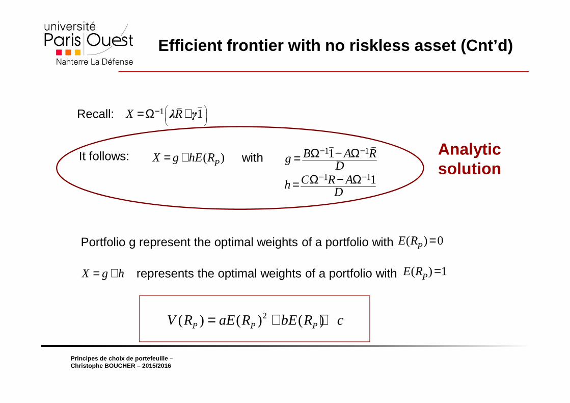
Recall: 1 1X R

−= Ω +λ γ

( )PX g hE R= + 1 1

1 1

1

1

B A RgD

C R AhD

− −

− −

Ω − Ω=

Ω − Ω=

with

Portfolio g represent the optimal weights of a portfolio with ( ) 0PE R =

X g h= + represents the optimal weights of a portfolio with ( ) 1PE R =

2( ) ( ) ( )P P PV R aE R bE R c= + +

It follows: Analytic solution



Characterization of frontier portfolios

51

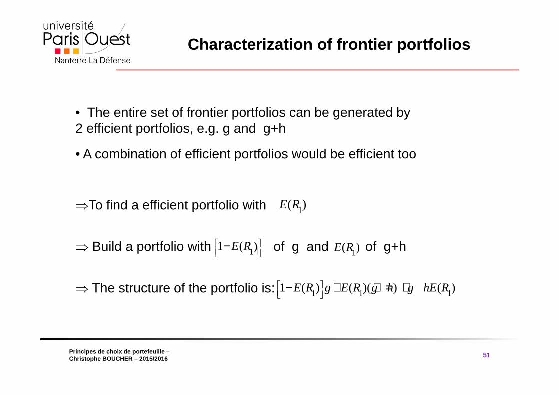
• The entire set of frontier portfolios can be generated by 2 efficient portfolios, e.g. g and g+h

• A combination of efficient portfolios would be efficient too

⇒To find a efficient portfolio with

⇒ Build a portfolio with of g and of g+h

⇒ The structure of the portfolio is:

1( )E R

11 ( )E R

−1( )E R

1 1 11 ( ) ( )( ) ( )E R g E R g h g hE R

− + + = +



3.5 Portfolio Diversification

52



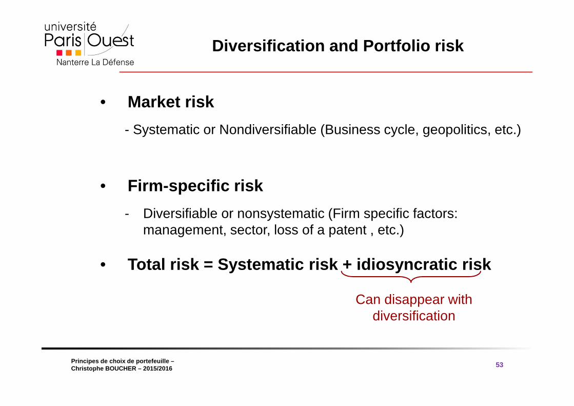
Diversification and Portfolio risk

53

• Market risk

- Systematic or Nondiversifiable (Business cycle, geopolitics, etc.)

• Firm -specific risk

- Diversifiable or nonsystematic (Firm specific factors: management, sector, loss of a patent , etc.)

• Total risk = Systematic risk + idiosyncratic risk

Can disappear with diversification



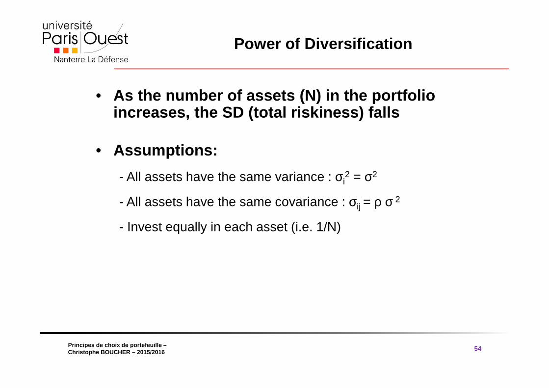
Power of Diversification

54

• As the number of assets (N) in the portfolio increases, the SD (total riskiness) falls

• Assumptions:

- All assets have the same variance : σi2 = σ2

- All assets have the same covariance : σij = ρ σ 2

- Invest equally in each asset (i.e. 1/N)



Power of Diversification

55

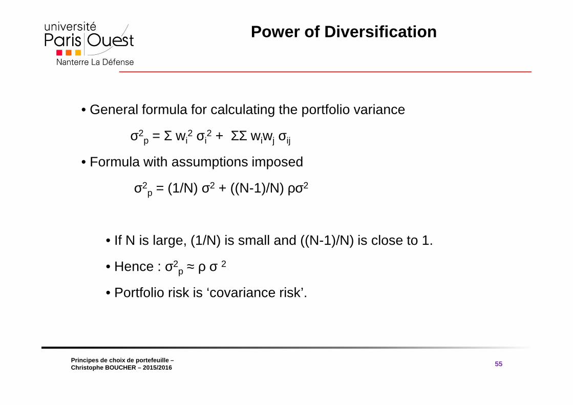
• General formula for calculating the portfolio variance

σ2p = Σ wi

2 σi2 + ΣΣ wiwj σij

• Formula with assumptions imposed

σ2p = (1/N) σ2 + ((N-1)/N) ρσ2

• If N is large, (1/N) is small and ((N-1)/N) is close to 1.

• Hence : σ2p ≈ ρ σ 2

• Portfolio risk is ‘covariance risk’.


transparents traduits par Vincent Dropsy Principes de choix de portefeuille –Christophe BOUCHER – 2015/2016 56

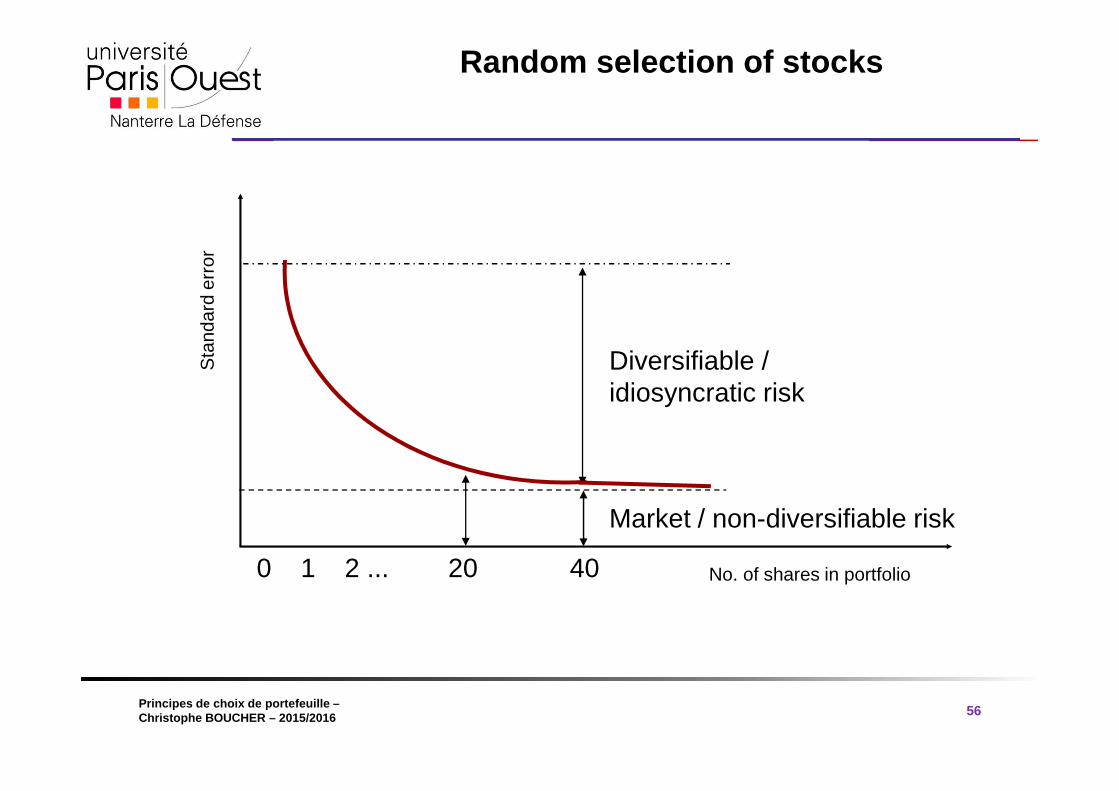
Sta

ndar

d er

ror

No. of shares in portfolio

Diversifiable / idiosyncratic risk

Market / non-diversifiable risk

20 400 1 2 ...

Random selection of stocks



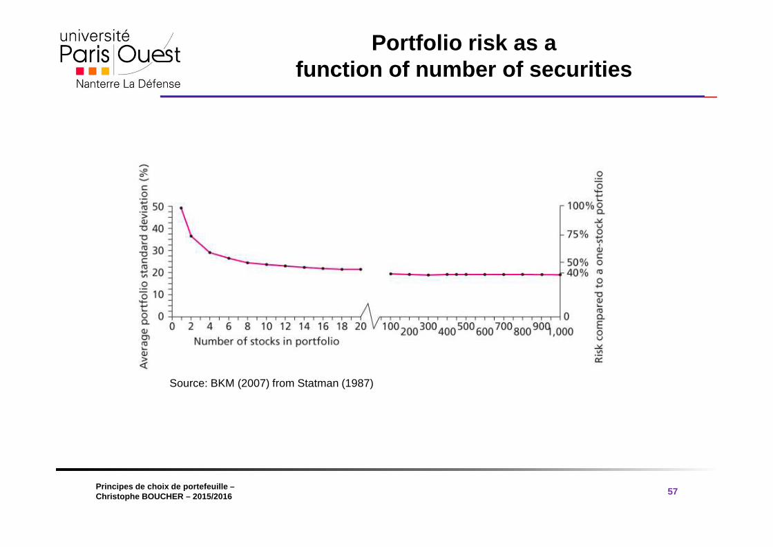
Portfolio risk as a function of number of securities

Source: BKM (2007) from Statman (1987)



Thank you for your attention…

See you next week

Documents

Principes de choix de portefeuille - Freeboucher.univ.free.fr/publis/cours/2015/CB_CPCh4_2015.pdf · ® 2009 Pearson Education France transparents traduits par Vincent Dropsy Principes