Embed Size (px)
Citation preview
Principal Component Analysis & Factor Analysis
Psych 818DeShon

Purpose
● Both are used to reduce the dimensionality of correlated measurements– Can be used in a purely exploratory fashion to
investigate dimensionality– Or, can be used in a quasi-confirmatory fashion to
investigate whether the empirical dimensionality is consistent with the expected or theoretical dimensionality
● Conceptually, very different analyses● Mathematically, there is substantial overlap
Principal Component Analysis
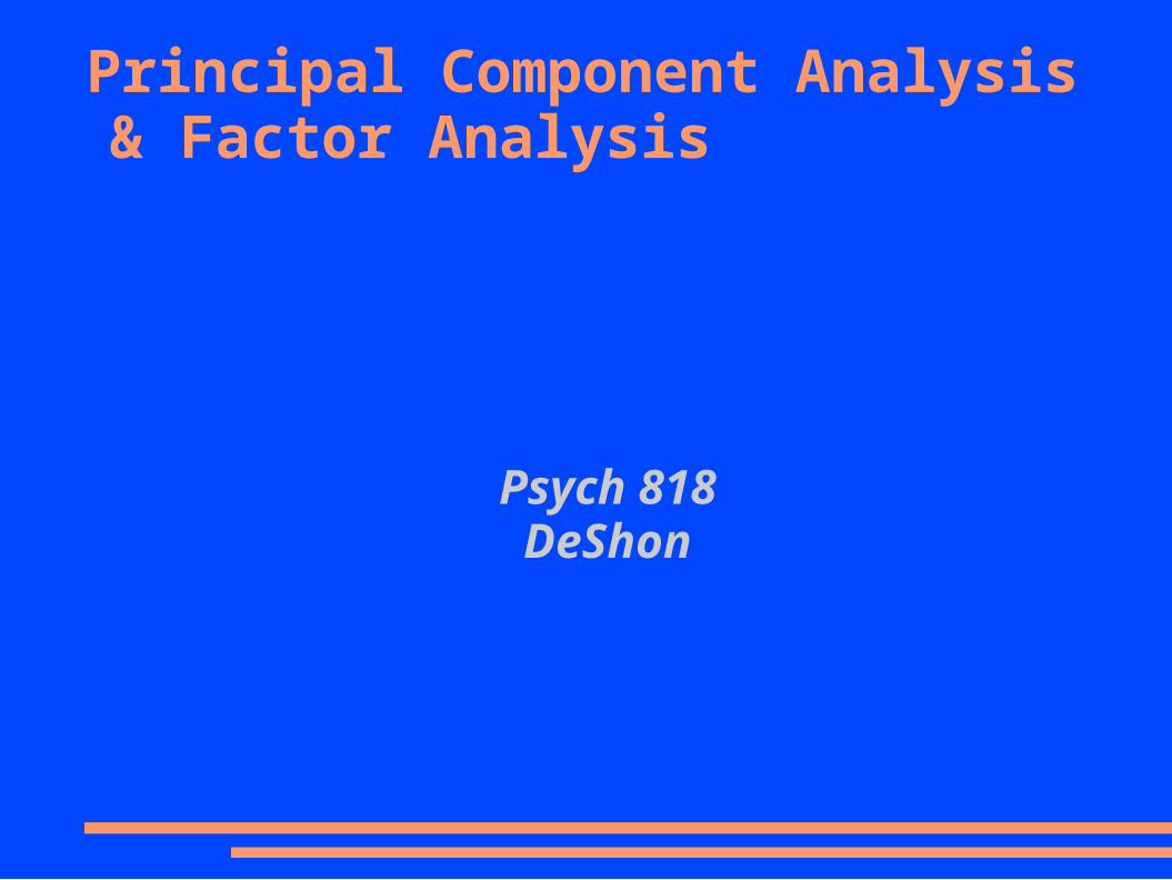
● Principal component analysis is conceptually and mathematically less complex – So, start here...
● First rule...– Don't interpret components as factors or latent
variables.– Components are simply weighted composite variables– They should be interpreted and called components or
composites
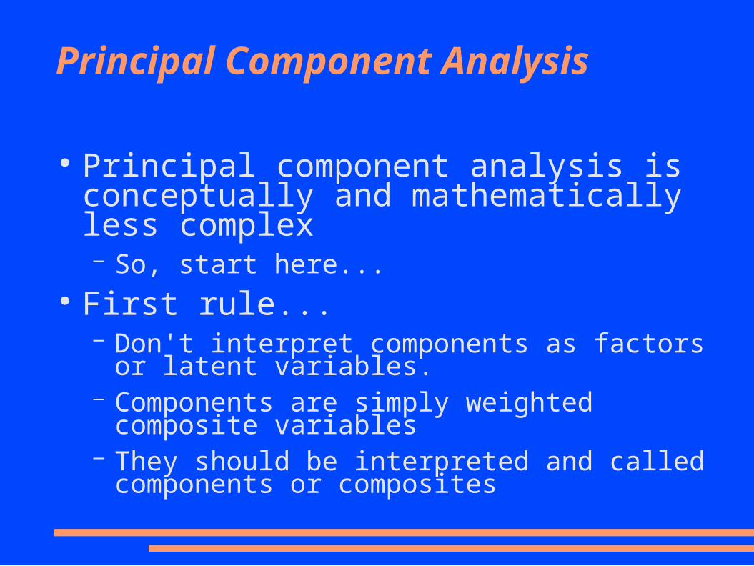
Principal Component Analysis
x1
x2
x3
x4
x5
x6
C1
C2
r = 0.0?
a11
a12
a13
a14
a15
a16
a26
a25
a24
a23
a22
a21
Principal Component Analysis
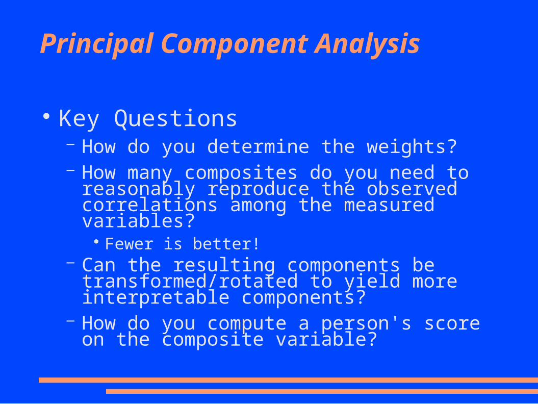
● Key Questions– How do you determine the weights?– How many composites do you need to reasonably
reproduce the observed correlations among the measured variables?
● Fewer is better!– Can the resulting components be transformed/rotated
to yield more interpretable components?– How do you compute a person's score on the
composite variable?
Conceptually...
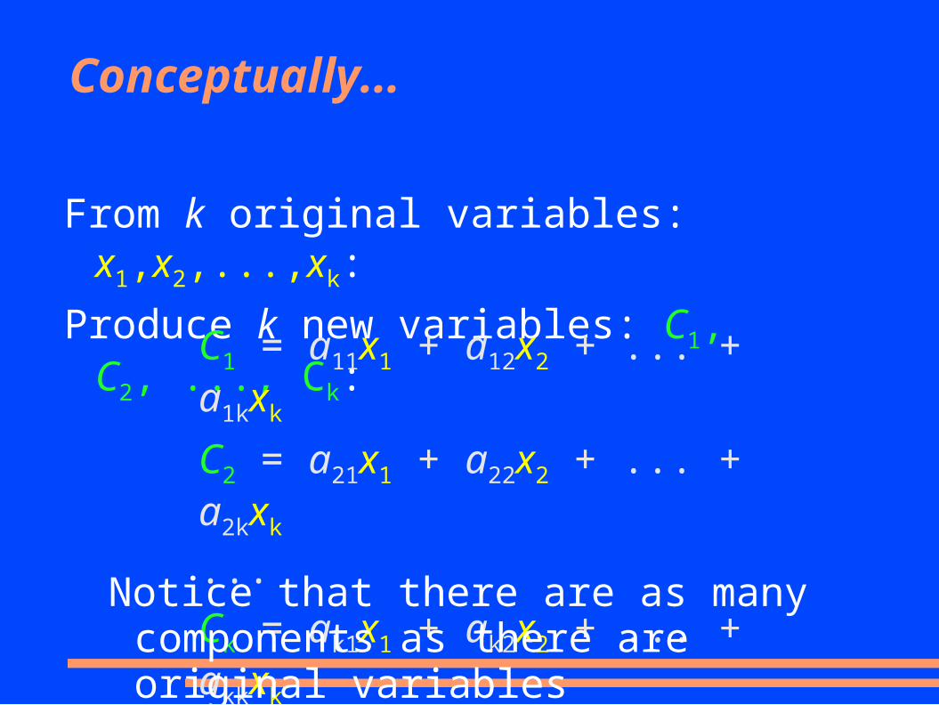
From k original variables: x1,x2,...,xk:
Produce k new variables: C1, C2, ..., Ck:
C1 = a11x1 + a12x2 + ... + a1kxk
C2 = a21x1 + a22x2 + ... + a2kxk
...
Ck = ak1x1 + ak2x2 + ... + akkxk
Notice that there are as many components as there are original variables
Conceptually...
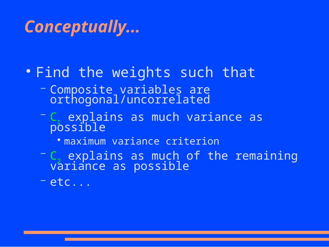
● Find the weights such that – Composite variables are orthogonal/uncorrelated– C
1 explains as much variance as possible
● maximum variance criterion– C
2 explains as much of the remaining variance as
possible– etc...
Conceptually...
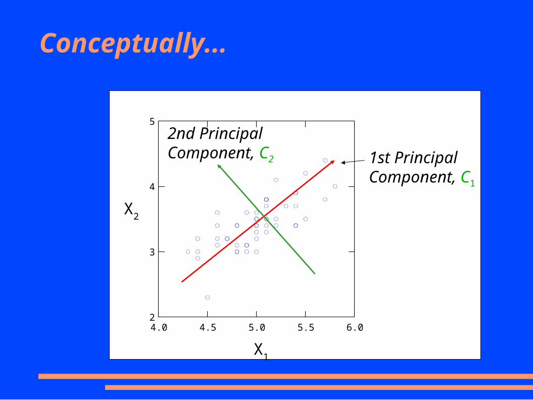
4.0 4.5 5.0 5.5 6.02
3
4
5
1st Principal Component, C1
2nd Principal Component, C2
X1
X2
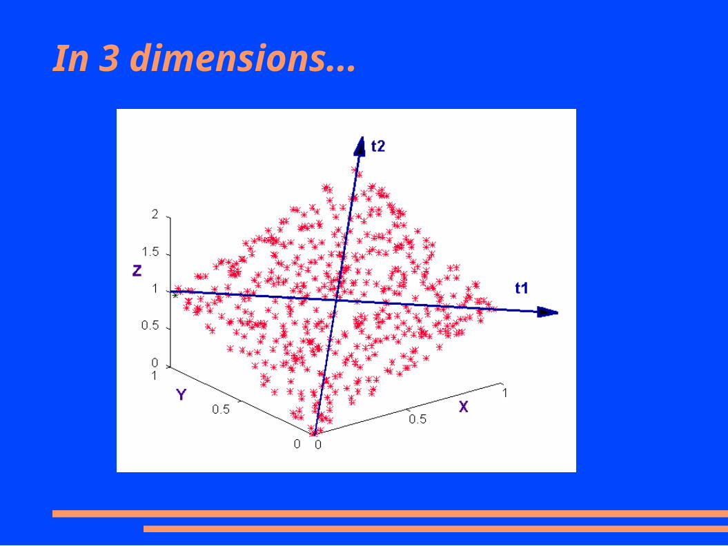
In 3 dimensions...
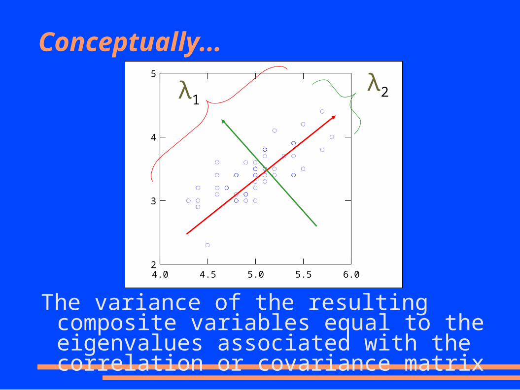
Conceptually...
The variance of the resulting composite variables equal to the eigenvalues associated with the correlation or covariance matrix
4.0 4.5 5.0 5.5 6.02
3
4
5
λ1λ2
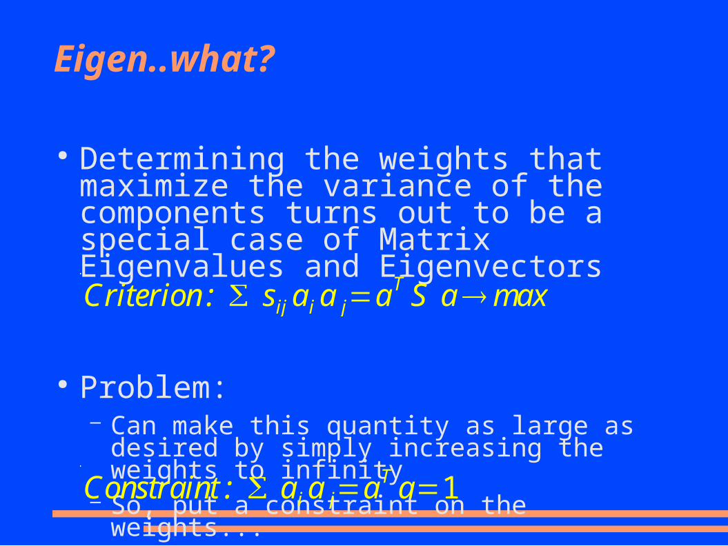
Eigen..what?
● Determining the weights that maximize the variance of the components turns out to be a special case of Matrix Eigenvalues and Eigenvectors
● Problem:– Can make this quantity as large as desired by simply
increasing the weights to infinity– So, put a constraint on the weights...
Criterion : sij a i a j=aT S a max
Constraint : ai a j=aT a=1
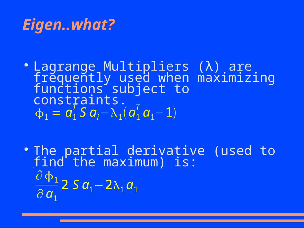
Eigen..what?
● Lagrange Multipliers (λ) are frequently used when maximizing functions subject to constraints.
● The partial derivative (used to find the maximum) is:
1 = a1T S a i−1a1
T a1−1
∂1
∂ a1
2 S a1−21 a1
Eigen..what?
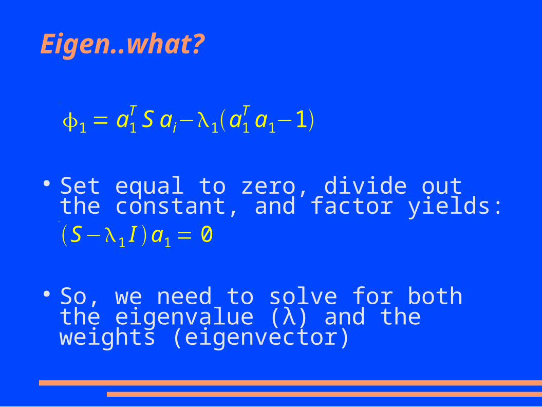
● Set equal to zero, divide out the constant, and factor yields:
● So, we need to solve for both the eigenvalue (λ) and the weights (eigenvector)
1 = a1T S a i−1a1
T a1−1
S−1 I a1 = 0
Eigen..what?
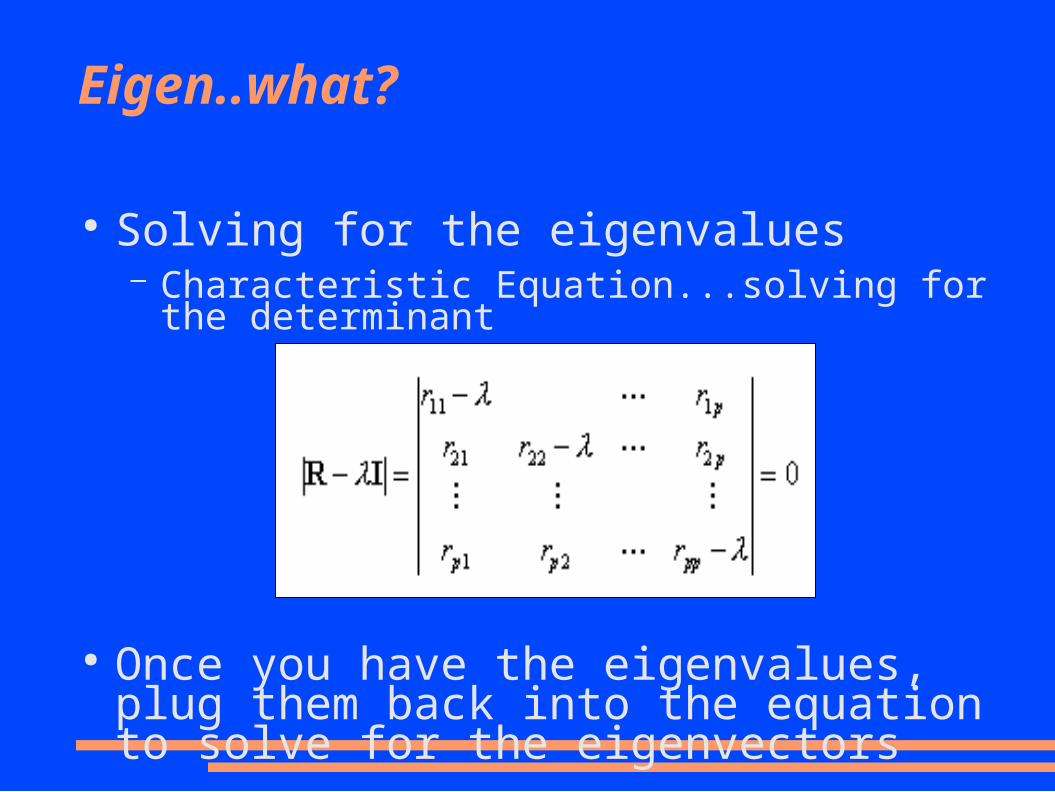
● Solving for the eigenvalues– Characteristic Equation...solving for the determinant
● Once you have the eigenvalues, plug them back into the equation to solve for the eigenvectors
Example (by Hand...)
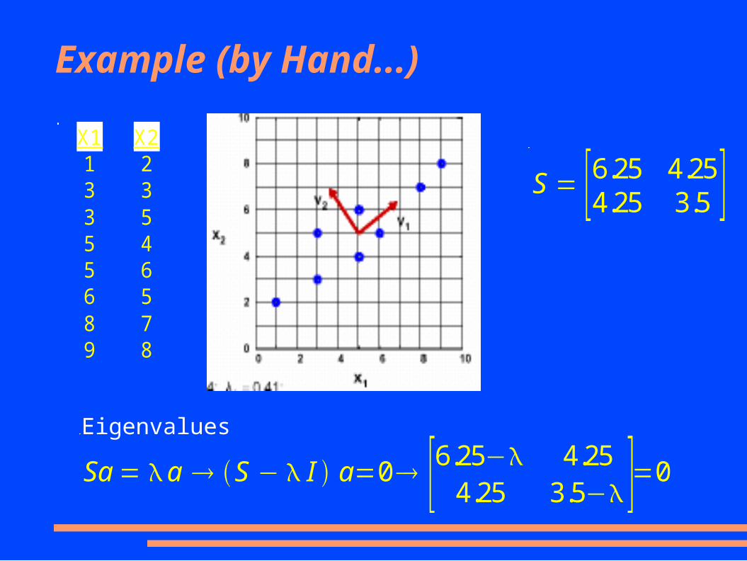
X1 X21 23 33 55 45 66 58 79 8
S = [6.25 4.254.25 3.5 ]
Sa = a S − I a=0 [6.25− 4.254.25 3.5− ]=0
Eigenvalues
Example (by Hand...)
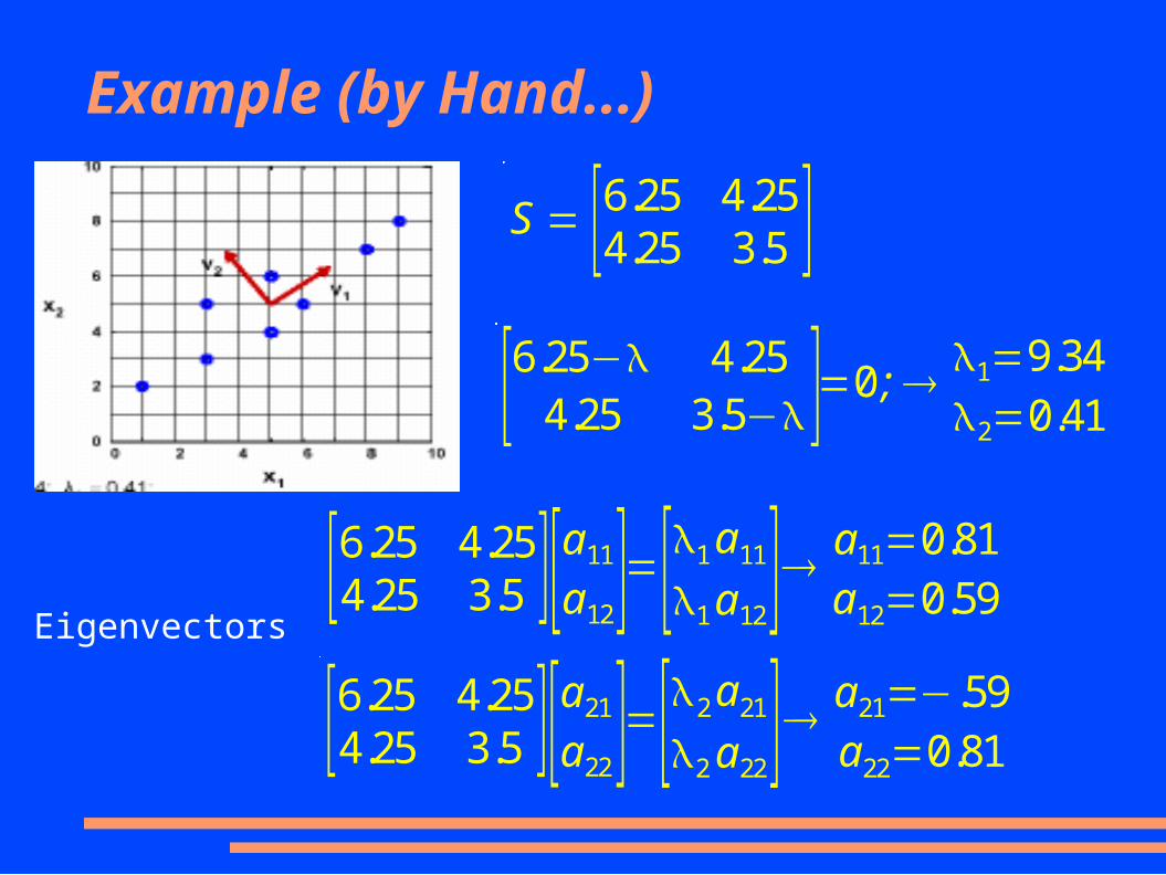
S = [6.25 4.254.25 3.5 ]
[6.25− 4.254.25 3.5− ]=0 ; 1=9.34
2=0.41
[6.25 4.254.25 3.5 ] [a11
a12 ]=[1 a11
1 a12] a11=0.81
a12=0.59
[6.25 4.254.25 3.5 ] [a21
a22 ]=[2 a21
2 a22] a21=−.59
a22=0.81
Eigenvectors
Stopping Rules
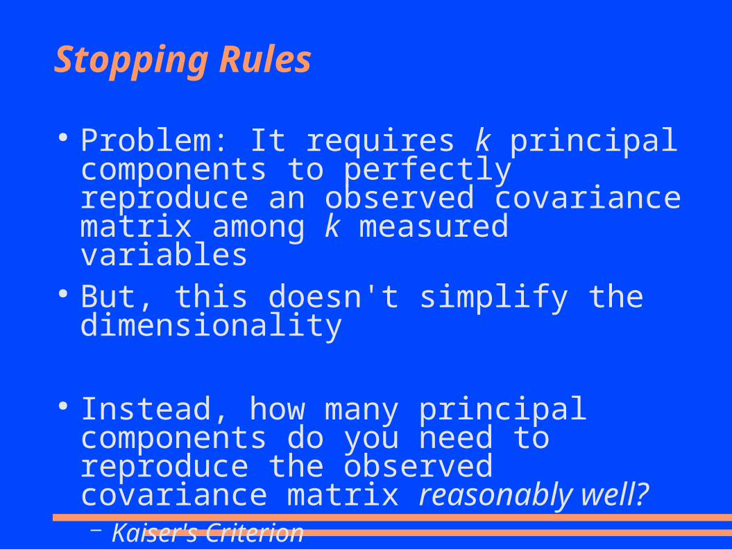
● Problem: It requires k principal components to perfectly reproduce an observed covariance matrix among k measured variables
● But, this doesn't simplify the dimensionality
● Instead, how many principal components do you need to reproduce the observed covariance matrix reasonably well?– Kaiser's Criterion
● If λj < 1 then component explains less variance than original variable (correlation matrix)
– Cattell's Scree Criterion
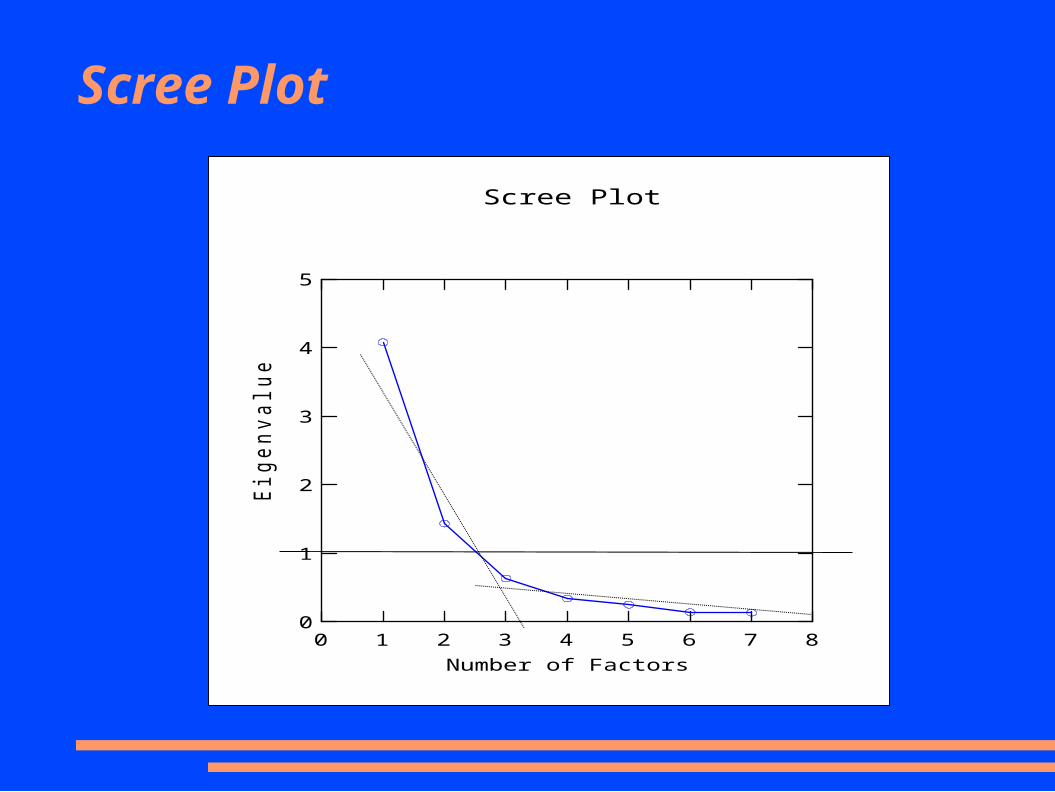
Scree Plot
Scree Plot
0 1 2 3 4 5 6 7 8Number of Factors
0
1
2
3
4
5E
igenvalu
e
Component Rotation
● The components have been achieved using a maximal variance criterion. – Good for prediction using the fewest possible
composites– Bad for understanding
● So, once the number of desired components has been determined, rotate them to a more understandable pattern/criterion– Simple Structure!
Simple Structure
● Thurstone, 1944– Each variable has at least one zero loading– Each factor in a factor matrix with k columns should
have k zero loadings– Each pair of columns in a factor matrix should have
several variables loading on one factor but not the other
– Each pair of columns should have a large proportion of variables with zero loadings in both columns
– Each pair of columns should only have a small proportion of variables with non zero loadings in both columns
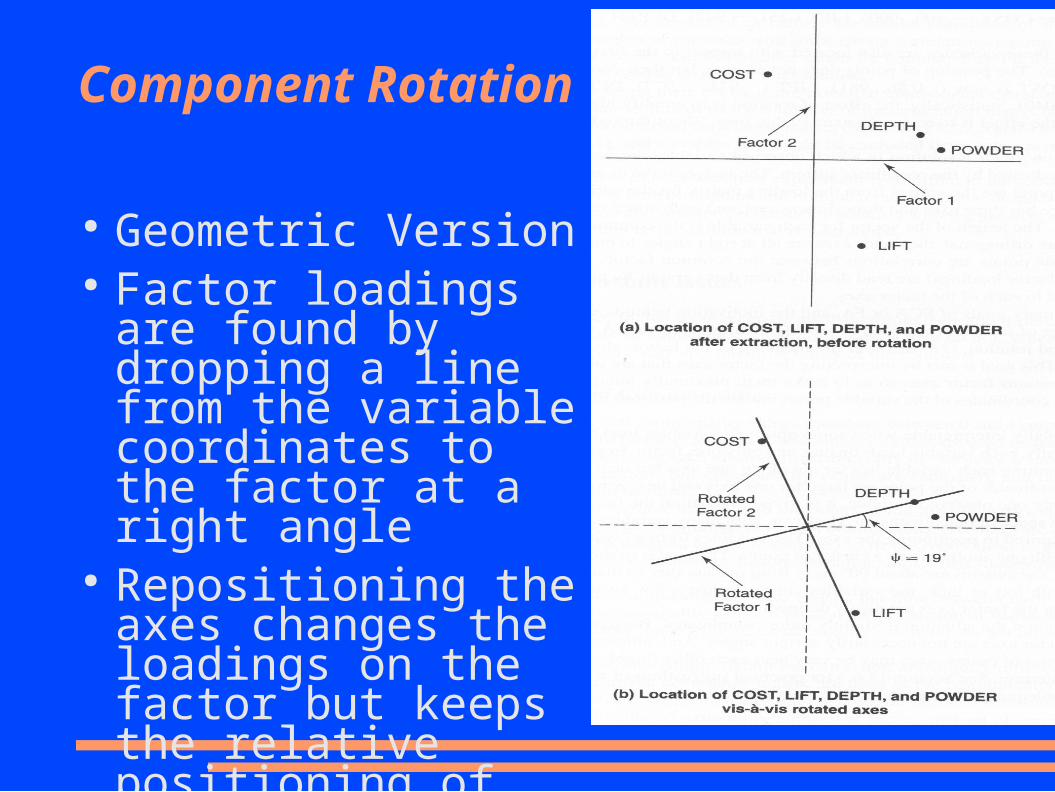
Component Rotation
● Geometric Version● Factor loadings are found
by dropping a line from the variable coordinates to the factor at a right angle
● Repositioning the axes changes the loadings on the factor but keeps the relative positioning of the points the same
Simple Structure Rotations
● Orthogonal vs. Oblique– Orthogonal rotation keeps factors un-correlated while
increasing the meaning of the factors– Oblique rotation allows the factors to correlate leading
to a conceptually clearer picture but a nightmare for explanation
Orthogonal Rotations
● Varimax – most popular– Simple structure by maximizing variance of loadings
within factors across variables– Makes large loading larger and small loadings smaller– Spreads the variance from first (largest) factor to other
smaller factors● Quartimax - Not used as often
– Opposite of Varimax– minimizes the number of factors needed to explain
each variable– often generates a general factor on which most
variables are loaded to a high or medium degree.
Orthogonal Rotations
● Equamax – Not popular– hybrid of the earlier two that tries to simultaneously
simplify factors and variables– compromise between Varimax and Quartimax criteria.
Oblique Rotations
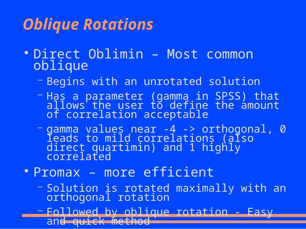
● Direct Oblimin – Most common oblique– Begins with an unrotated solution – Has a parameter (gamma in SPSS) that allows the user
to define the amount of correlation acceptable– gamma values near -4 -> orthogonal, 0 leads to mild
correlations (also direct quartimin) and 1 highly correlated
● Promax – more efficient– Solution is rotated maximally with an orthogonal
rotation– Followed by oblique rotation - Easy and quick method– Orthogonal loadings are raised to powers in order to
drive down small loadings - Simple structure
Component Loadings
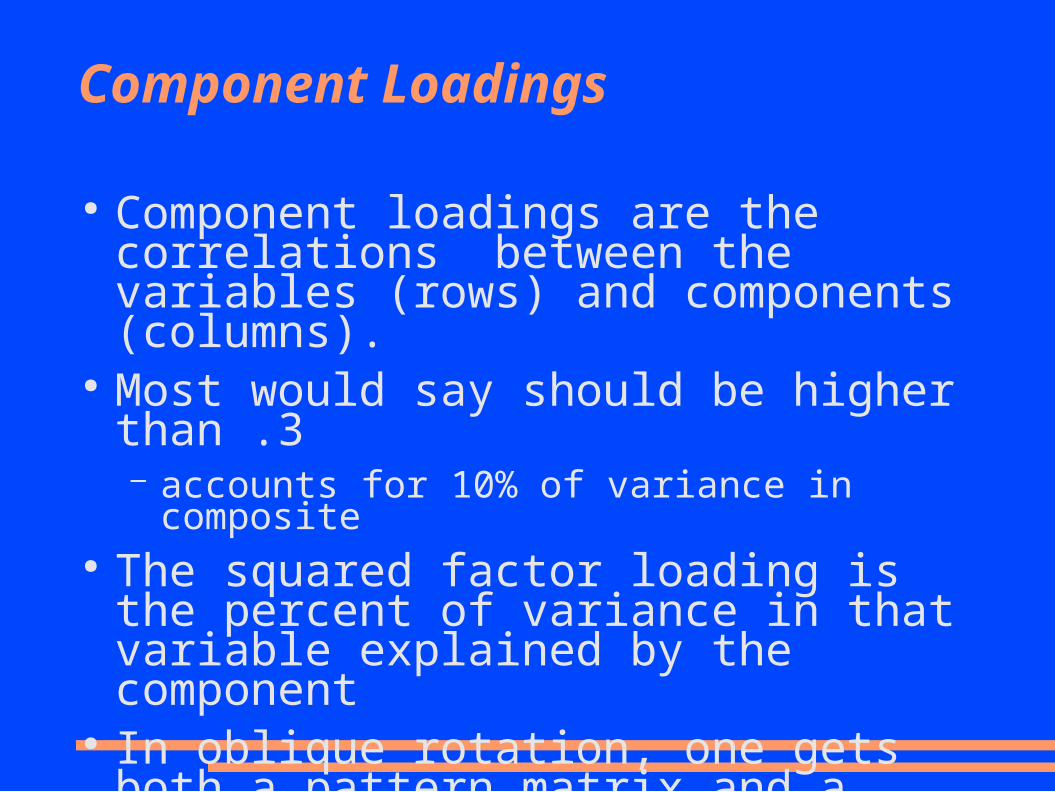
● Component loadings are the correlations between the variables (rows) and components (columns).
● Most would say should be higher than .3– accounts for 10% of variance in composite
● The squared factor loading is the percent of variance in that variable explained by the component
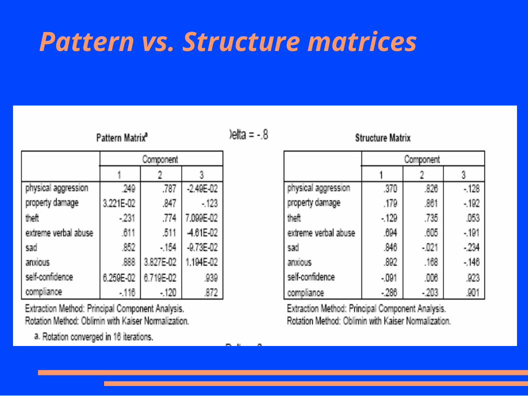
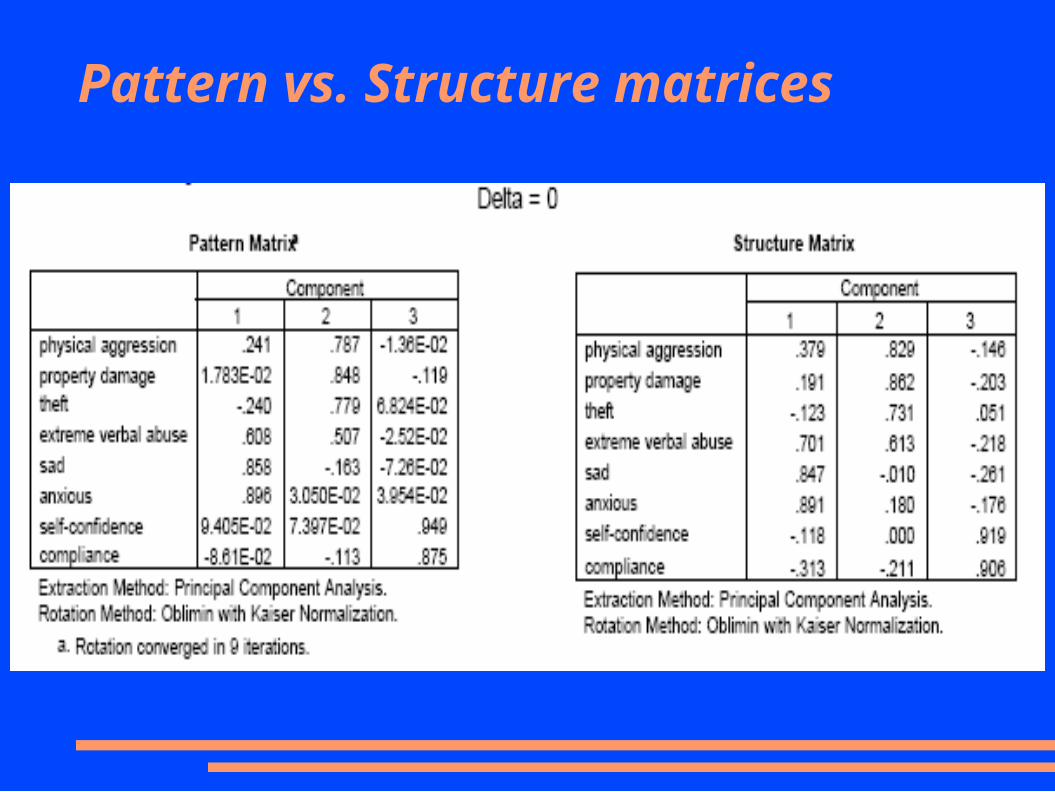
● In oblique rotation, one gets both a pattern matrix and a structure matrix
Component Loadings
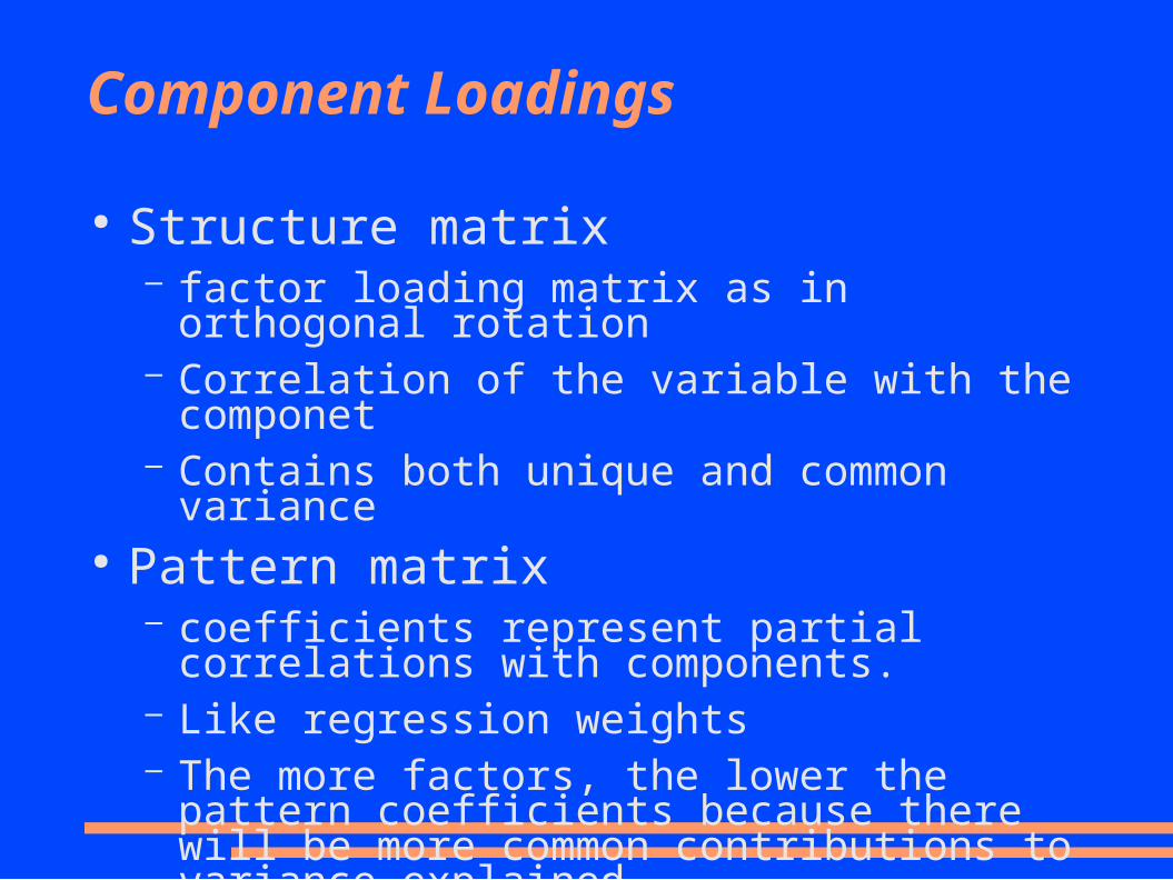
● Structure matrix– factor loading matrix as in orthogonal rotation– Correlation of the variable with the componet– Contains both unique and common variance
● Pattern matrix– coefficients represent partial correlations with
components.– Like regression weights– The more factors, the lower the pattern coefficients
because there will be more common contributions to variance explained
Component Loadings
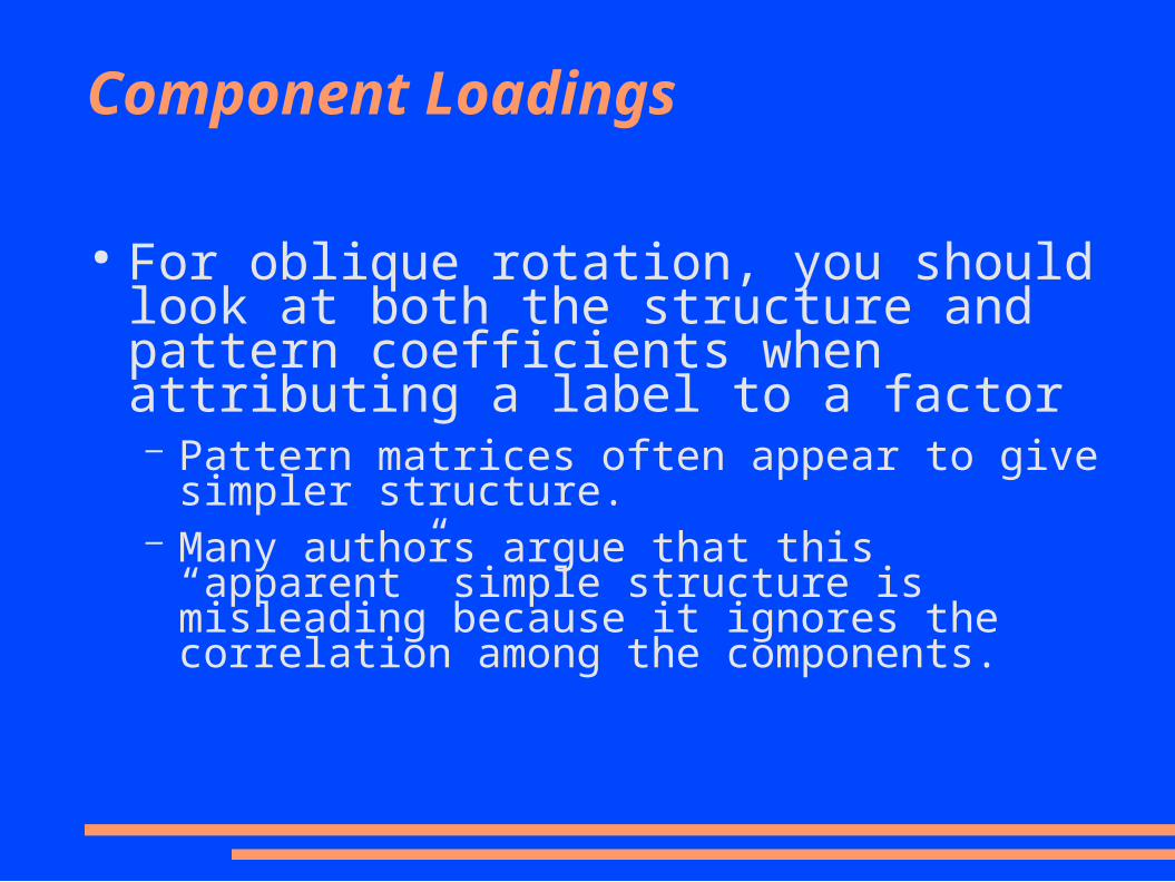
● For oblique rotation, you should look at both the structure and pattern coefficients when attributing a label to a factor– Pattern matrices often appear to give simpler structure.– Many authors argue that this “apparent” simple
structure is misleading because it ignores the correlation among the components.
Pattern vs. Structure matrices
Pattern vs. Structure matrices
Component Scores
● A person's score on a composite is simply the weighted sum of the variable scores
● A component score is a person’s score on that composite variable -- when their variable values are applied as:
PC1 = a11X1 + a 21X2 + … + a k1Xk
– The weights are the eigenvalues.● These scores can be used as variables in further
analyses (e.g., regression)
Covariance or Correlation Matrix?
● Covariance Matrix:– Variables must be in same units– Emphasizes variables with most variance– Mean eigenvalue ≠1.0
● Correlation Matrix:– Variables are standardized (mean 0.0, SD 1.0)– Variables can be in different units– All variables have same impact on analysis– Mean eigenvalue = 1.0
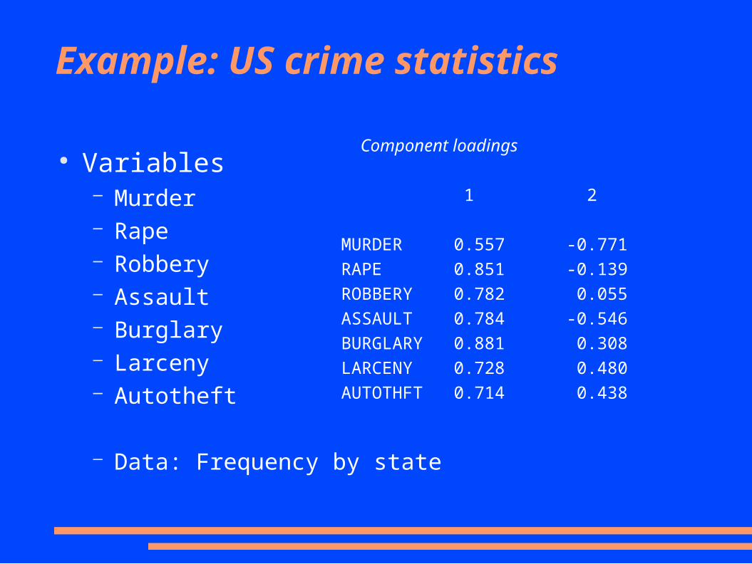
Example: US crime statistics
● Variables– Murder– Rape – Robbery – Assault– Burglary – Larceny – Autotheft
– Data: Frequency by state
Component loadings
1 2
MURDER 0.557 -0.771
RAPE 0.851 -0.139
ROBBERY 0.782 0.055
ASSAULT 0.784 -0.546
BURGLARY 0.881 0.308
LARCENY 0.728 0.480
AUTOTHFT 0.714 0.438
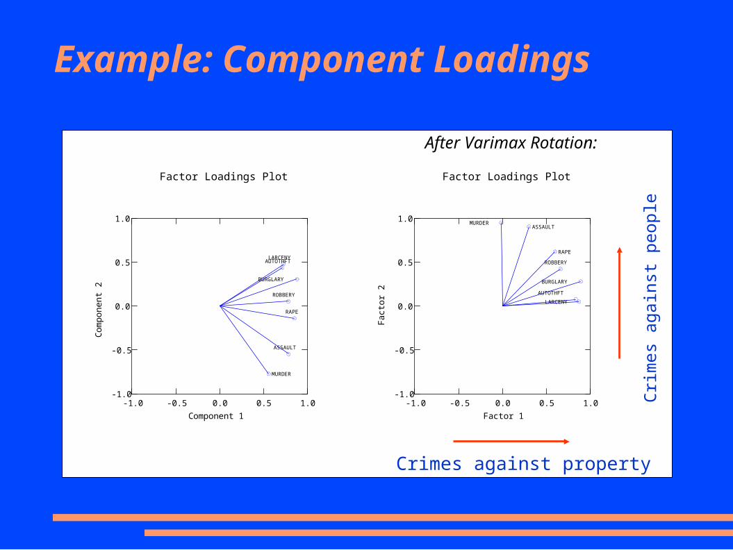
Example: Component Loadings
Factor Loadings Plot
-1.0 -0.5 0.0 0.5 1.0Component 1
-1.0
-0.5
0.0
0.5
1.0
Co
mp
on
en
t 2
MURDER
AUTOTHFTLARCENY
BURGLARY
RAPE
ASSAULT
ROBBERY
Factor Loadings Plot
-1.0 -0.5 0.0 0.5 1.0Factor 1
-1.0
-0.5
0.0
0.5
1.0
Fa
cto
r 2
MURDERASSAULT
RAPE
BURGLARY
LARCENYAUTOTHFT
ROBBERY
After Varimax Rotation:
Crimes against property
Crim
es a
gain
st p
eopl
e
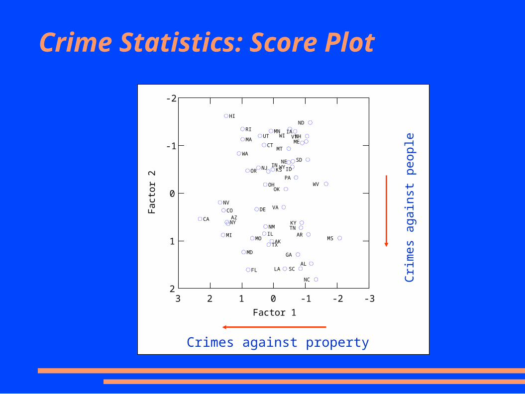
Crime Statistics: Score Plot
-3-2-10123Factor 1
-2
-1
0
1
2
Fa
cto
r 2
MS
WV
NC
AL
ND
AR
SD
NHME
VT
KYTN
SC
GA
PA
IA
NEWY
WI
ID
MT
OK
LA
VA
KS
CA
NV
MI
CO
HI
NYAZ
WA
RI
MA
MD
OR
FL
MO
DE
NJ
UT
CT
IL
OH
NM
IN
TX
MN
AK
Crim
es a
gain
st p
eopl
e
Crimes against property
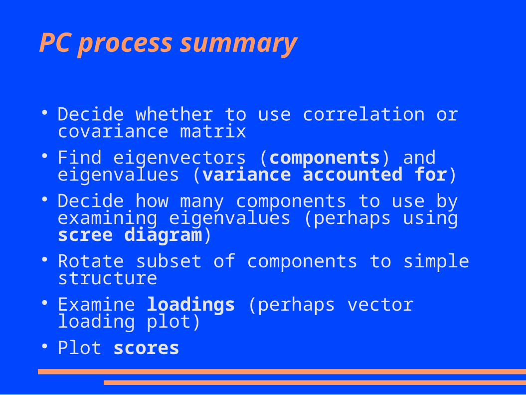
PC process summary
● Decide whether to use correlation or covariance matrix ● Find eigenvectors (components) and eigenvalues
(variance accounted for)● Decide how many components to use by examining
eigenvalues (perhaps using scree diagram)● Rotate subset of components to simple structure● Examine loadings (perhaps vector loading plot)● Plot scores
PCA Terminology & Relations
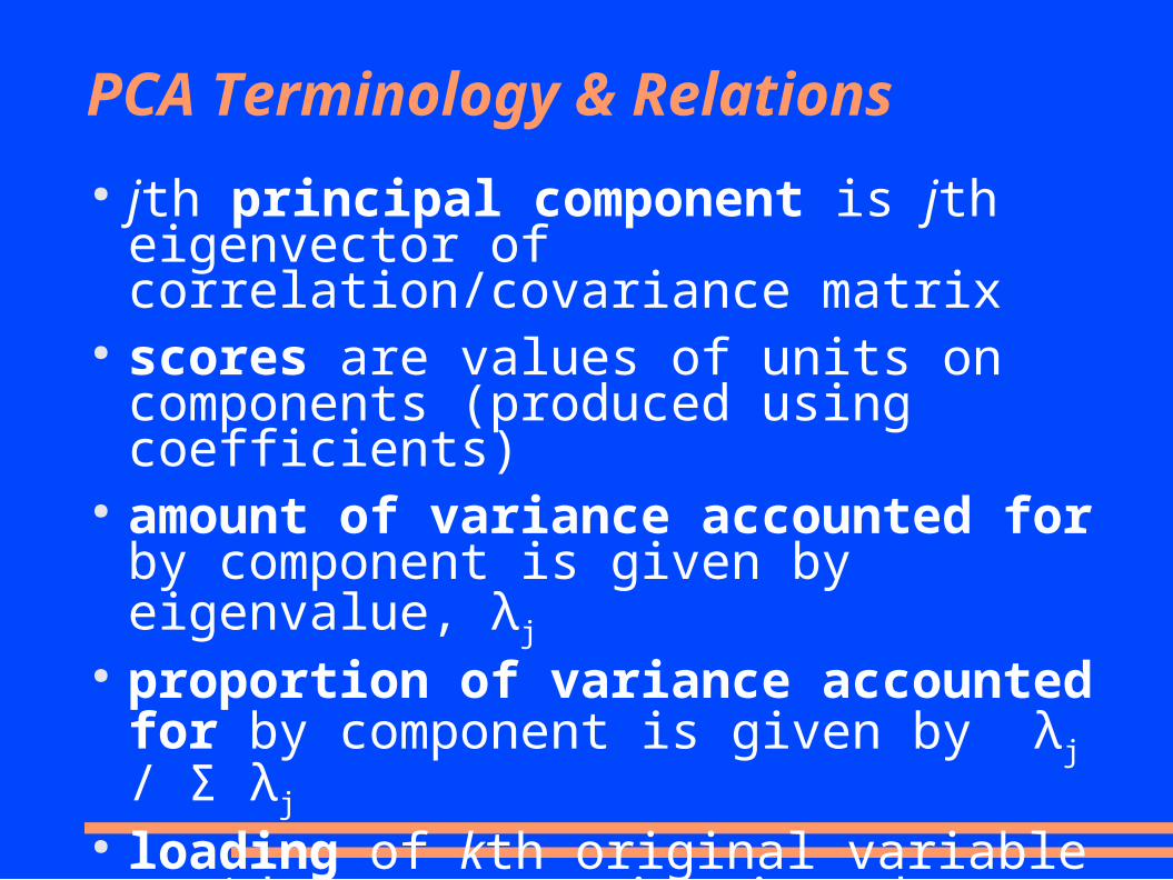
● jth principal component is jth eigenvector ofcorrelation/covariance matrix
● scores are values of units on components (produced using coefficients)
● amount of variance accounted for by component is given by eigenvalue, λj
● proportion of variance accounted for by component is given by λj / Σ λj
● loading of kth original variable on jth component is given by ajk√λj --correlation between variable and component
PCA Relations
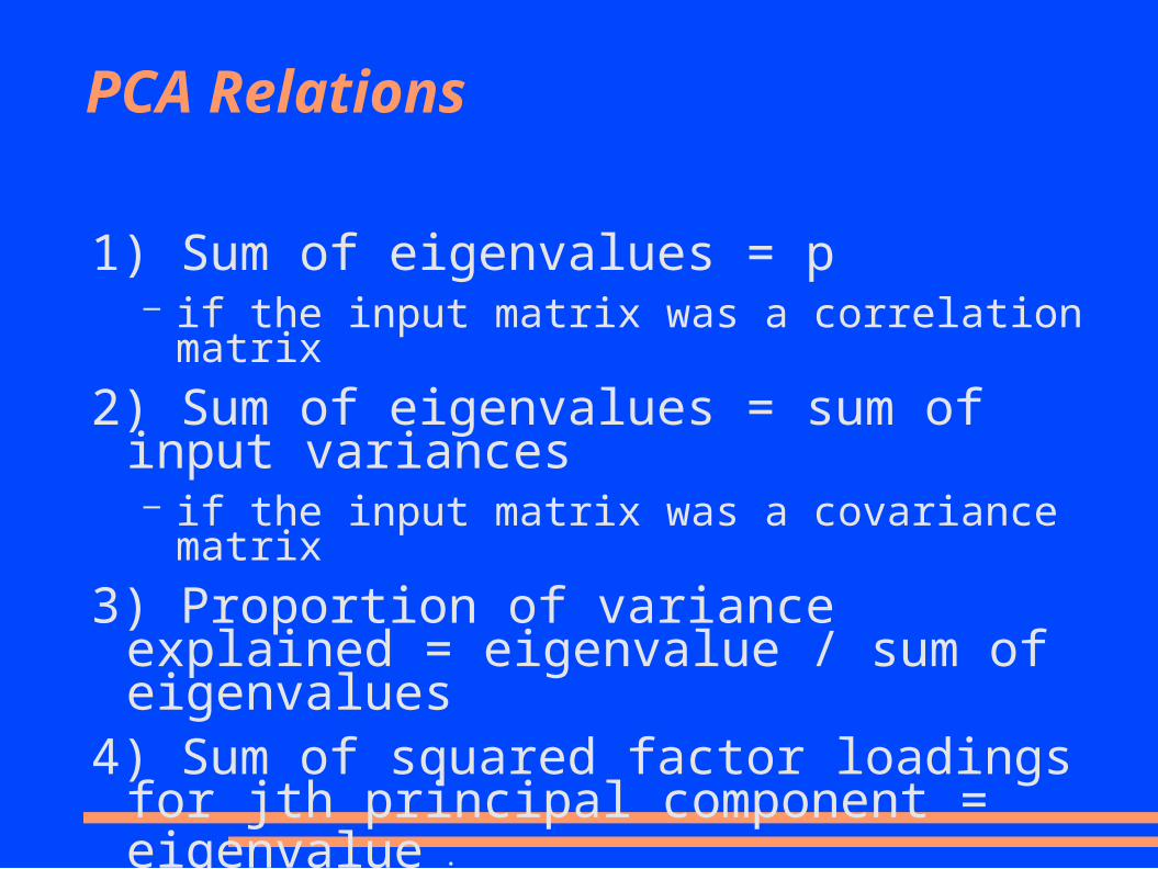
1) Sum of eigenvalues = p– if the input matrix was a correlation matrix
2) Sum of eigenvalues = sum of input variances– if the input matrix was a covariance matrix
3) Proportion of variance explained = eigenvalue / sum of eigenvalues
4) Sum of squared factor loadings for jth principal component = eigenvalue
j
PCA Relations
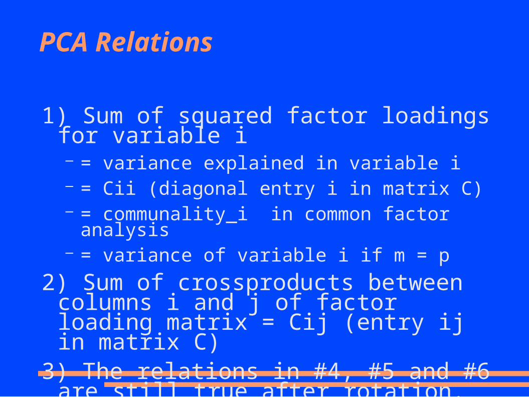
1) Sum of squared factor loadings for variable i– = variance explained in variable i– = Cii (diagonal entry i in matrix C)– = communality_i in common factor analysis– = variance of variable i if m = p
2) Sum of crossproducts between columns i and j of factor loading matrix = Cij (entry ij in matrix C)
3) The relations in #4, #5 and #6 are still true after rotation.
Factor Analysis Model
x1
x2
x3
x4
x5
x6
C1
C2
r = 0.0?
e1
e2
e3
e4
e5
e6
Factor Analysis
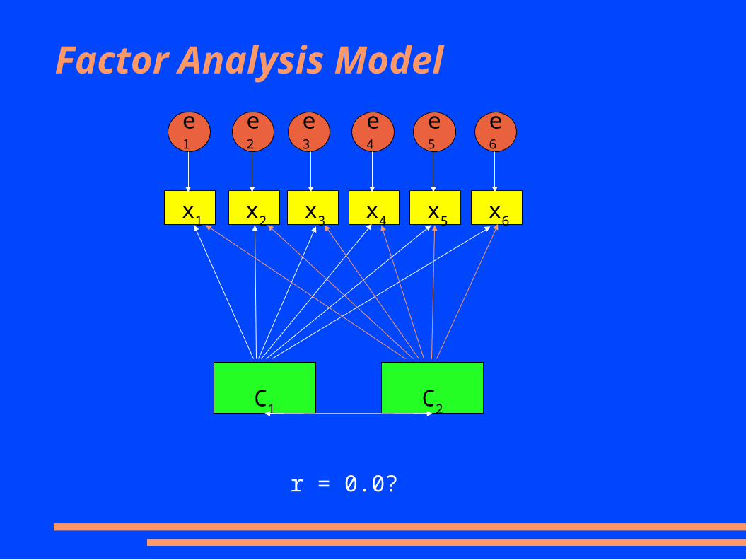
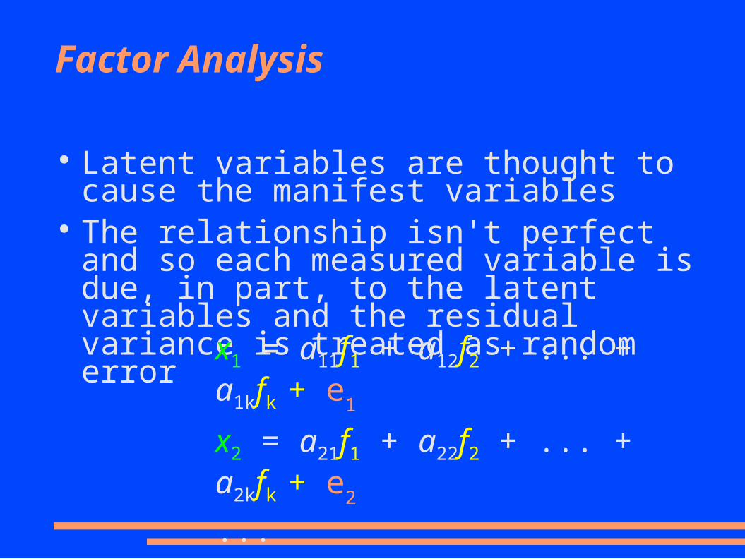
● Latent variables are thought to cause the manifest variables
● The relationship isn't perfect and so each measured variable is due, in part, to the latent variables and the residual variance is treated as random error
x1 = a11f1 + a12f2 + ... + a1kfk + e1
x2 = a21f1 + a22f2 + ... + a2kfk + e2
...
xp = ap1f1 + ap2f2 + ... + apkfk + e3
Model Identification
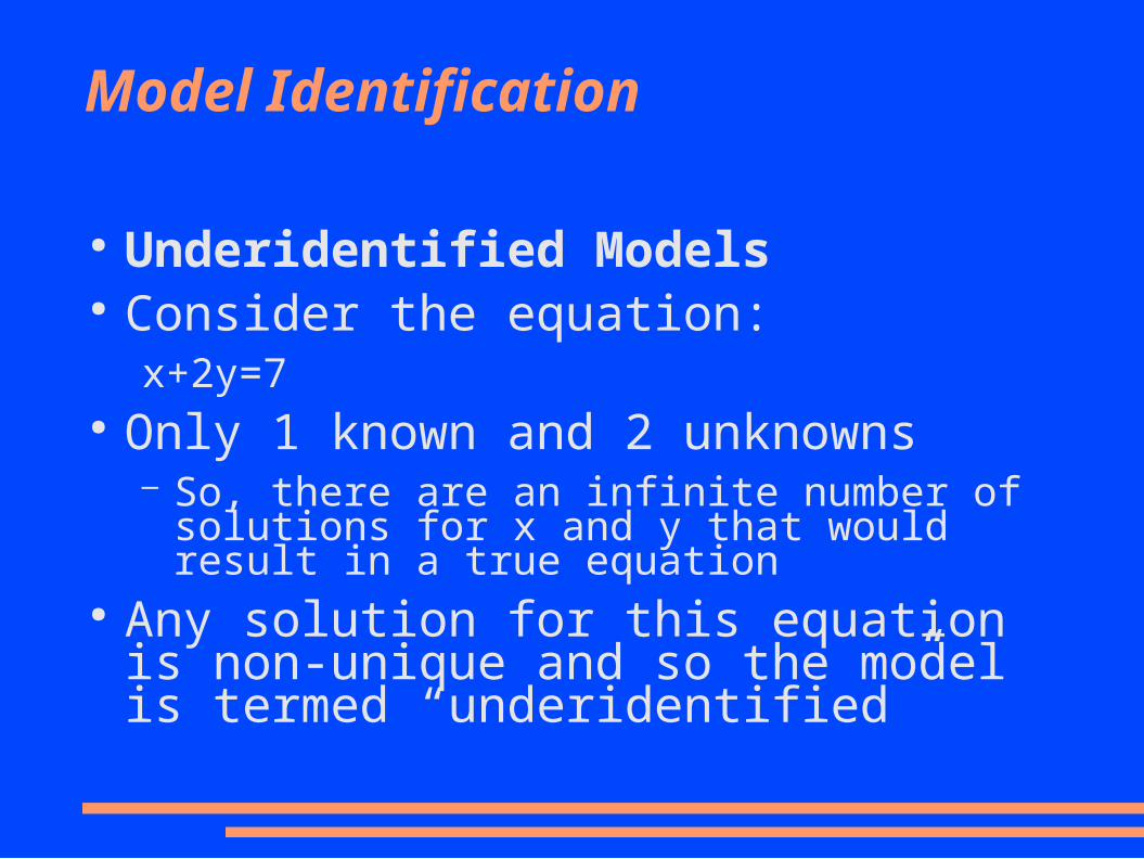
● Underidentified Models● Consider the equation:
x+2y=7● Only 1 known and 2 unknowns
– So, there are an infinite number of solutions for x and y that would result in a true equation
● Any solution for this equation is non-unique and so the model is termed “underidentified”
Model Identification
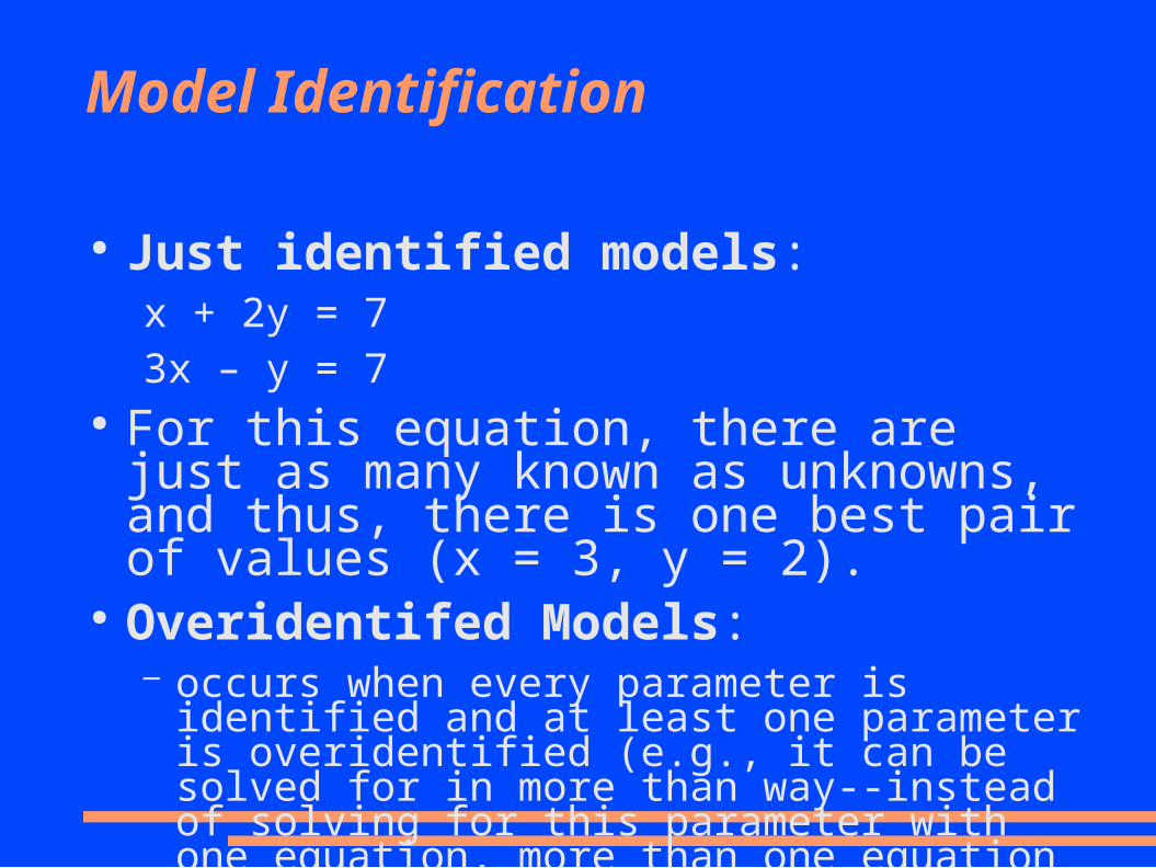
● Just identified models:x + 2y = 73x – y = 7
● For this equation, there are just as many known as unknowns, and thus, there is one best pair of values (x = 3, y = 2).
● Overidentifed Models:– occurs when every parameter is identified and at least
one parameter is overidentified (e.g., it can be solved for in more than way--instead of solving for this parameter with one equation, more than one equation will generate this parameter estimate).
Model Identification
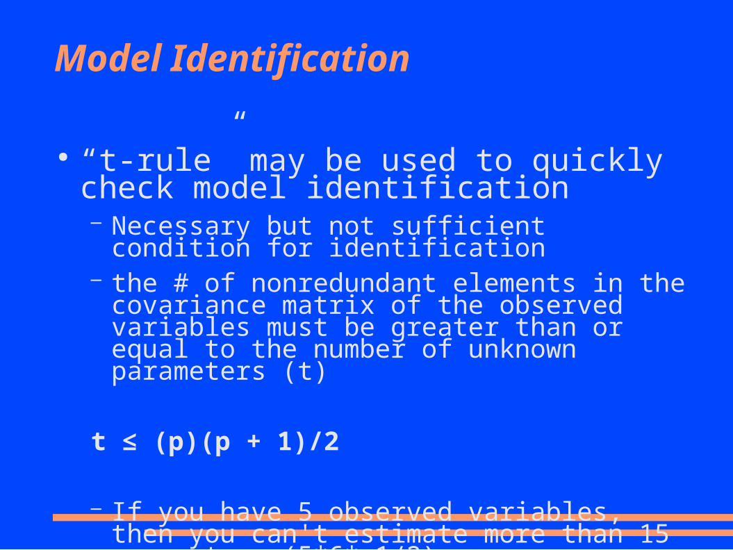
● “t-rule” may be used to quickly check model identification– Necessary but not sufficient condition for identification– the # of nonredundant elements in the covariance
matrix of the observed variables must be greater than or equal to the number of unknown parameters (t)
t ≤ (p)(p + 1)/2
– If you have 5 observed variables, then you can't estimate more than 15 parameters (5*6* 1/2)
Is the Factor model identified?
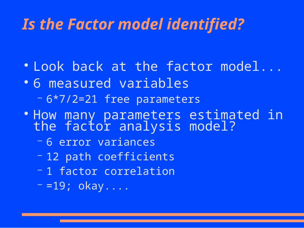
● Look back at the factor model...● 6 measured variables
– 6*7/2=21 free parameters● How many parameters estimated in the factor
analysis model?– 6 error variances– 12 path coefficients– 1 factor correlation– =19; okay....
Is the Factor model identified?
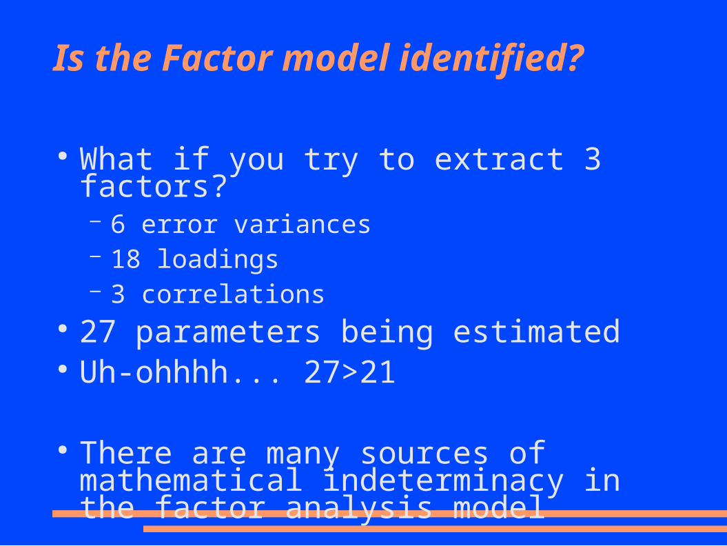
● What if you try to extract 3 factors?– 6 error variances– 18 loadings– 3 correlations
● 27 parameters being estimated● Uh-ohhhh... 27>21
● There are many sources of mathematical indeterminacy in the factor analysis model
A useful dodge...
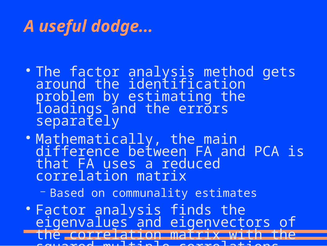
● The factor analysis method gets around the identification problem by estimating the loadings and the errors separately
● Mathematically, the main difference between FA and PCA is that FA uses a reduced correlation matrix– Based on communality estimates
● Factor analysis finds the eigenvalues and eigenvectors of the correlation matrix with the squared multiple correlations each variable with other variables on the main diagonal
Estimating Communality
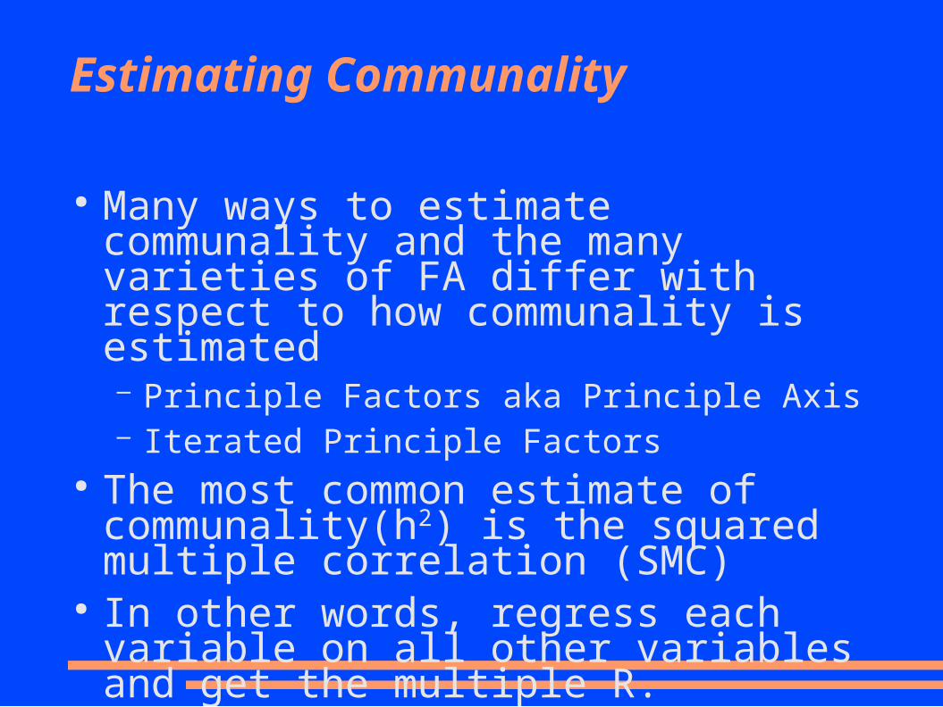
● Many ways to estimate communality and the many varieties of FA differ with respect to how communality is estimated– Principle Factors aka Principle Axis– Iterated Principle Factors
● The most common estimate of communality(h2) is the squared multiple correlation (SMC)
● In other words, regress each variable on all other variables and get the multiple R.x
i2 = b
o + b
1x
i1 + b
2x
i3 + ... + b
px
ip
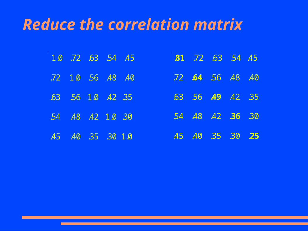
Reduce the correlation matrix
1.0 .72 .63 .54 .45
.72 1.0 .56 .48 .40
.63 .56 1.0 .42 .35
.54 .48 .42 1.0 .30
.45 .40 .35 .30 1.0
.81 .72 .63 .54 .45
.72 .64 .56 .48 .40
.63 .56 .49 .42 .35
.54 .48 .42 .36 .30
.45 .40 .35 .30 .25
FA Analysis
● Now, just perform a PCA on the reduced correlation matrix
● Re-estimate communalities based on the factor solution
Common problems in FA
● The communality estimates are just that...estimates.
● These estimates can often result in impossible results.– Communality estimates greater than 1.0– Error variance estimates less than 0.0
● Collectively referred to as “Heywood Cases”● When encountered, the model does not fit.
– Simplify the model or reduce the number of variables being analyzed.
Factor Scores
● Unlike PCA, a person's score on the latent variable is indeterminant– Two unknowns (latent true score and error) but only
one observed score for each person● Can't compute the factor score as you can in
PCA.● Instead you have to estimate the person's factor
score.
Differences between PCA and FA
● Unless you have lots of error (very low communalities) you will get virtually identical results when you perform these two analyses
● I always do both● I've only seen a discrepancy one or two times
– Change FA model (number of factors extracted) or estimate communality differently or reduce the number of variables being factored
Some Guidelines
● Factors need at least three variables with high loadings or should not be interpreted– Since the vars won't perform as expected you should
probably start out with 6 to 10 variables per factor.● If the loadings are low, you will need more
variables, 10 or 20 per factor may be required. ● The larger the n, the larger the number of vars
per factor, and the larger the loadings, the better– Strength in one of these areas can compensate for
weakness in another – Velicer, W. F., & Fava, J. L. (1998). Effects of
variable and subject sampling on factor pattern recovery. Psychological Methods, 3, 231-251.
Some Guidelines
● Large N, high h2, and high overdetermination (each factor having at least three or four high loadings and simple structure) increase your chances of reproducing the population factor pattern
● When communalities are high (> .6), you should be in good shape even with N well below 100
● With communalities moderate (about .5) and the factors well-determined, you should have 100 to 200 subjects
Some Guidelines
● With communalities low (< .5) but high overdetermination of factors (not many factors, each with 6 or 7 high loadings), you probably need well over 100 subjects.
● With low communalities and only 3 or 4 high loadings on each, you probably need over 300 subjects.
● With low communalities and poorly determined factors, you will need well over 500 subjects.– MacCallum, R. C., Widaman, K. F., Zhang, S., &
Hong, S. (1999). Sample size in factor analysis. Psychological Methods, 4, 84-99.

Example...