Pricing options with VG model using FFT - UCLAitkin/publications/virginia2005.pdf · 2 Pricing European option 6 3 Carr-Madan’s FFT approach and the VG model 6 ... investigate various

Pricing options with VG model using FFT

Andrey Itkin

October 21, 2005

Revision: 1.0

Moscow State Aviation UniversityDepartment of applied mathematics and physics

[email protected]

Summary

We discuss various analytic and numerical methods that have been used to get option priceswithin a framework of the VG model. We show that some popular methods, for instance, Carr-Madan’s FFT method [1] could blow up for certain values of the model parameters even for anEuropean vanilla option. Alternative methods - one originally proposed by Lewis, and Black-Scholes-wise method are considered that seem to work fine for any value of the VG parameters.Test examples are given to demonstrate efficiency of these methods. Convergency of all methodsis also discussed.

1

Contents

1 Introduction 4

2 Pricing European option 6

3 Carr-Madan’s FFT approach and the VG model 6

4 Lewis’s regularization 10

5 Black-Scholes-wise method 12

6 Convergency and performance 16

7 Conclusion 18

List of Figures

1 European option values in VG model at T = 0.02yrs, K = 90, σ = 0.01 obtainedwith FRFT. . . . . . . . . . . . . . . . . . . . . . . . . . . . . . . . . . . . . . . . . 7

2 European option values in VG model at T = 0.02yrs, K = 90, σ = 0.01 obtainedwith the adaptive integration. . . . . . . . . . . . . . . . . . . . . . . . . . . . . . . 7

3 European option values in VG model at T = 0.02yrs, K = 90, σ = 0.01 obtainedwith FFT. . . . . . . . . . . . . . . . . . . . . . . . . . . . . . . . . . . . . . . . . . 8

4 European option values in VG model at T = 1.0yrs, K = 90, σ = 1.0 obtained withthe FFT. . . . . . . . . . . . . . . . . . . . . . . . . . . . . . . . . . . . . . . . . . 8

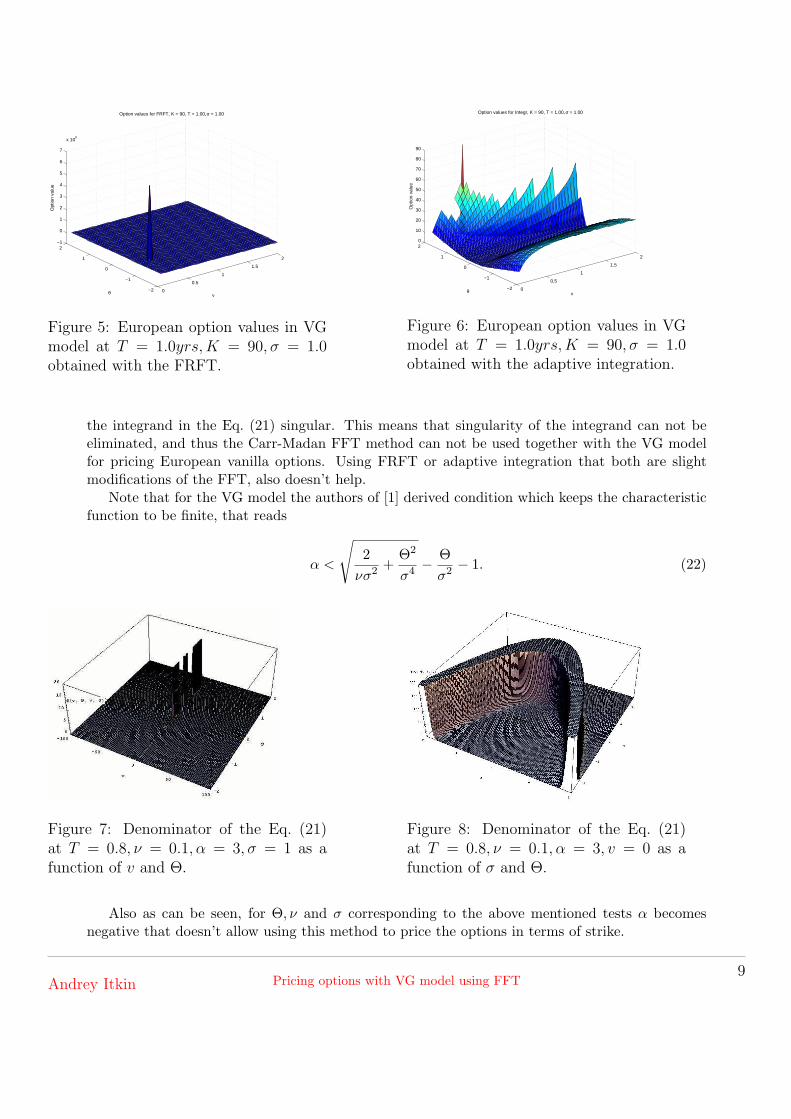
5 European option values in VG model at T = 1.0yrs, K = 90, σ = 1.0 obtained withthe FRFT. . . . . . . . . . . . . . . . . . . . . . . . . . . . . . . . . . . . . . . . . 9

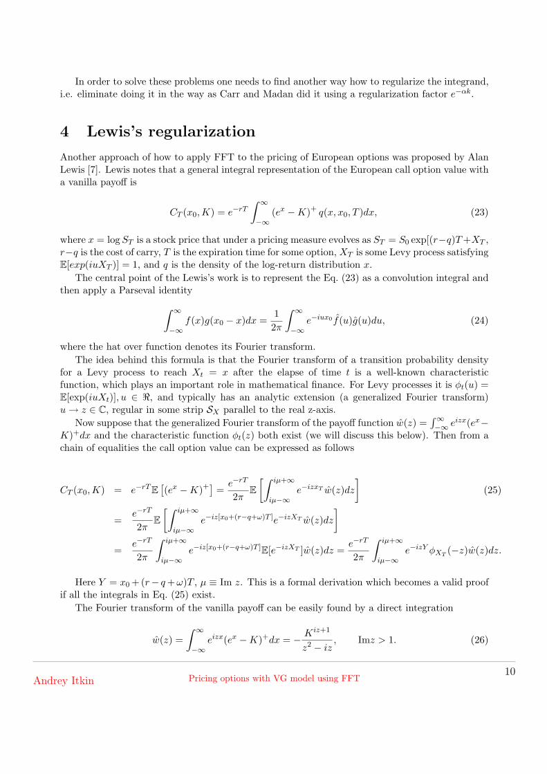
6 European option values in VG model at T = 1.0yrs, K = 90, σ = 1.0 obtained withthe adaptive integration. . . . . . . . . . . . . . . . . . . . . . . . . . . . . . . . . . 9

7 Denominator of the Eq. (21) at T = 0.8, ν = 0.1, α = 3, σ = 1 as a function of v andΘ. . . . . . . . . . . . . . . . . . . . . . . . . . . . . . . . . . . . . . . . . . . . . . 9

8 Denominator of the Eq. (21) at T = 0.8, ν = 0.1, α = 3, v = 0 as a function of σ andΘ. . . . . . . . . . . . . . . . . . . . . . . . . . . . . . . . . . . . . . . . . . . . . . 9

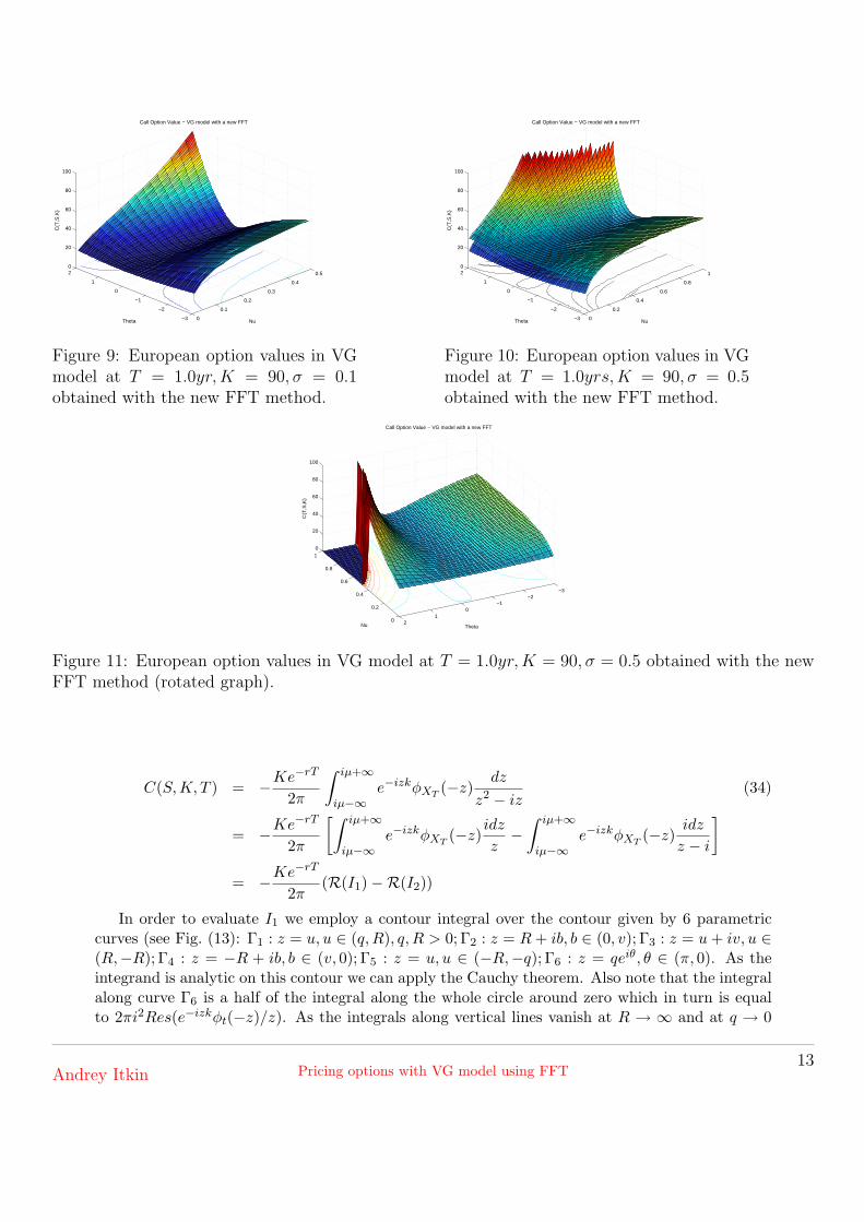
9 European option values in VG model at T = 1.0yr,K = 90, σ = 0.1 obtained withthe new FFT method. . . . . . . . . . . . . . . . . . . . . . . . . . . . . . . . . . . 13

10 European option values in VG model at T = 1.0yrs, K = 90, σ = 0.5 obtained withthe new FFT method. . . . . . . . . . . . . . . . . . . . . . . . . . . . . . . . . . . 13

11 European option values in VG model at T = 1.0yr,K = 90, σ = 0.5 obtained withthe new FFT method (rotated graph). . . . . . . . . . . . . . . . . . . . . . . . . . 13

12 The difference between the European call option values for the VG model obtainedwith Carr-Madan FFT method and the new FFT method. Parameters of the testare: S = 100, T = 0.5yr, σ = 0.2, ν = 0.1,Θ = −0.33, r = q = 0. at various strikes). 14

13 Integration contour for R(I1) . . . . . . . . . . . . . . . . . . . . . . . . . . . . . . 14

Andrey Itkin Pricing options with VG model using FFT2

14 European option values in VG model. Difference between the Carr-Madan solutionand Black-Scholes-wise solution with D1,2(u = 0) at T = 1.0yr, σ = 0.1, θ = 0.1, ν =0.1 . . . . . . . . . . . . . . . . . . . . . . . . . . . . . . . . . . . . . . . . . . . . . 16

15 European option values in VG model. Difference between the Carr-Madan solutionand Black-Scholes-wise solution with D1,2(u = ε) at T = 1.0yr, σ = 0.1, θ = 0.1, ν =0.1 . . . . . . . . . . . . . . . . . . . . . . . . . . . . . . . . . . . . . . . . . . . . . 16

16 Convergency of the Black-Scholes-wise method. Difference between the option priceobtained with N = 8192, and that with N = 4096, 1024, 512, 256 . . . . . . . . . . 17

17 Convergency of the Lewis method. Difference between the option price obtainedwith N = 8192, and that with N = 4096, 1024, 512, 256 . . . . . . . . . . . . . . . . 17

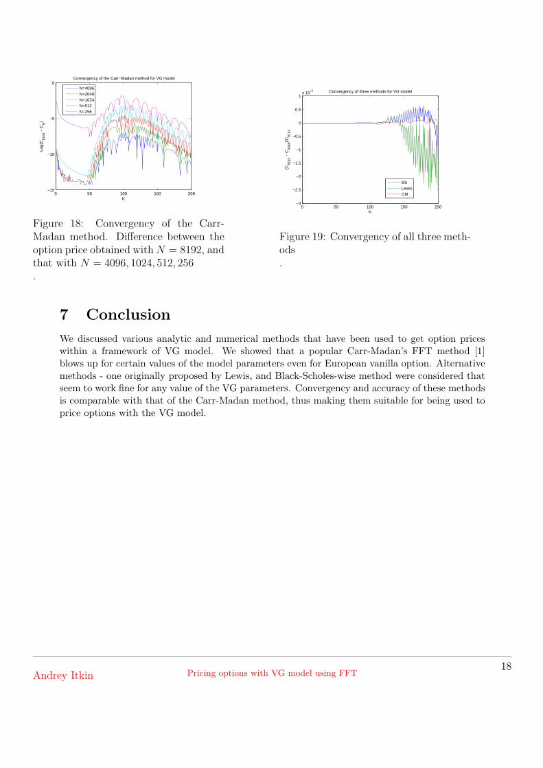
18 Convergency of the Carr-Madan method. Difference between the option price ob-tained with N = 8192, and that with N = 4096, 1024, 512, 256 . . . . . . . . . . . . 18

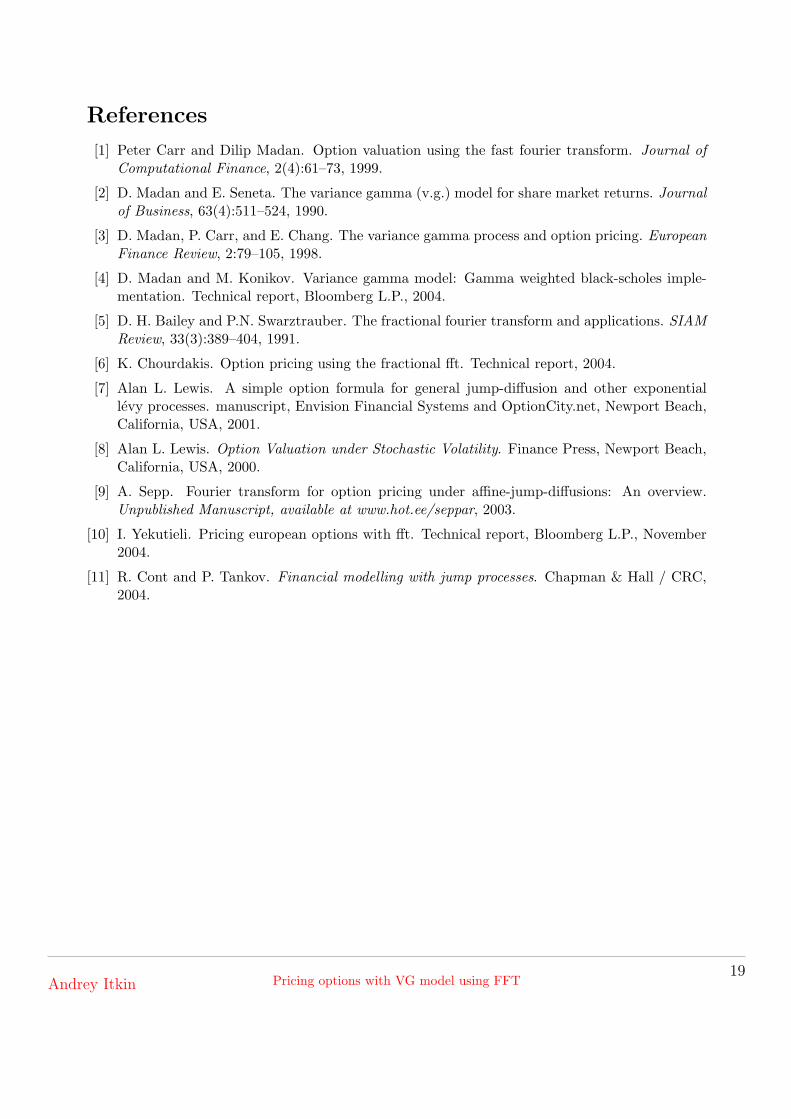
19 Convergency of all three methods . . . . . . . . . . . . . . . . . . . . . . . . . . . . 18


1 Introduction

This paper summarizes some results of work originally initiated by Peter Carr. It supposes toinvestigate various numerical and analytical methods of option pricing using VG model in orderto find out which algorithm is most efficient.

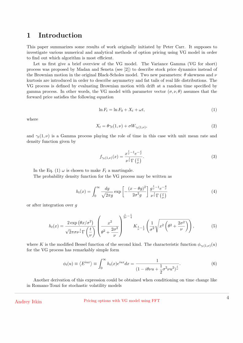
Let us first give a brief overview of the VG model. The Variance Gamma (VG for short)process was proposed by Madan and Seneta (see [2]) to describe stock price dynamics instead ofthe Brownian motion in the original Black-Scholes model. Two new parameters: θ skewness and νkurtosis are introduced in order to describe asymmetry and fat tails of real life distributions. TheVG process is defined by evaluating Brownian motion with drift at a random time specified bygamma process. In other words, the VG model with parameter vector (σ, ν, θ) assumes that theforward price satisfies the following equation

ln Ft = lnF0 + Xt + ωt, (1)

whereXt = θγt(1, ν) + σWγt(1,ν), (2)

and γt(1, ν) is a Gamma process playing the role of time in this case with unit mean rate anddensity function given by

fγt(1,ν)(x) =x

tν−1e−

xν

νtν Γ

(tν

) . (3)

In the Eq. (1) ω is chosen to make Ft a martingale.The probability density function for the VG process may be written as

ht(x) =∫ ∞

0

dg√2πg

exp[−(x− θg)2

2σ2g

]g

tν−1e−

gν

νtν Γ

(tν

) (4)

or after integration over g

ht(x) =2 exp

(θx/σ2

)√

2πσνtν Γ

(t

ν

)

x2

θ2 +2σ2

ν

t2ν− 1

4

K tν− 1

2

(1σ2

√x2

(θ2 +

2σ2

ν

)), (5)

where K is the modified Bessel function of the second kind. The characteristic function φγt(1,ν)(u)for the VG process has remarkably simple form

φt(u) ≡ ⟨Eiux

⟩ ≡∫ ∞

0ht(x)eiuxdx =

1

(1− iθνu +12σ2νu2)

tν

. (6)

Another derivation of this expression could be obtained when conditioning on time change likein Romano-Touzi for stochastic volatility models


φγt(1,ν)(u) = E[eiuγt(1,ν)] =∫ ∞

0eiuxfγt(1,ν)(x)dx =

∫ ∞

0eiux x

tν−1e−

xν

νtν Γ

(tν

) dx

=∫ ∞

0

xtν−1e−

x(1−iuν)ν

νtν Γ

(tν

) dx

= (1− iuν)−tν

∫ ∞

0

(x(1− iuν))tν−1e−

x(1−iuν)ν

νtν Γ

(tν

) d(x(1− iuν))

= (1− iuν)−tν

∫ ∞

0

ytν−1e−

yν

νtν Γ

(tν

) dy = (1− iuν)−tν . (7)

φXt(u) = E[eiuXt ] = E[E[eiuXt | γt(1, ν)]] = E[E[eiu(θγt(1,ν)+σWγt(1,ν)) | γt(1, ν)]]

= E[eiuθγt(1,ν)− 12u2σ2γt(1,ν)] = E[ei(uθ+i 1

2u2σ2)γt(1,ν)]

= φγt(1,ν)(uθ + i12u2σ2) =

(1− iθνu +

12σ2νu2

)− tν

. (8)

Now, to prevent arbitrage, we need Ft be a martingale, and, since Ft is already an independentincrement process, all we need is

E[Ft] = F0, (9)

or

E[F0eXt+ωt] = F0φXt(−i)eωt = F0. (10)

This tells us that

ω = − ln φXt(−i)t

= −−tν ln

(1− θν − 1

2σ2ν)

t=

1ν

ln(

1− θν − 12σ2ν

). (11)

Note that from the definition of ω above, in order to have a risk neutral measure for VG model,its parameters must obey an inequality:

1ν

> θ +σ2

2. (12)

Note that risk neutral parameters θ, ν, σ do not have to be equal to their statistical counterparts.Accordingly, the characteristic function of the xT ≡ log ST VG process is

φ(u) =S0e

(r−q+ω)T

(1− iθνu +

12σ2νu2

)Tν

. (13)

Statistical parameters of VG distribution may be calculated from the historical data on stockprices. In particular we have to find the values of the parameters θ∗, ν∗ and σ∗ such that thefolloiwng expression is maximized:


n∏

j=1

hτj (xj), (14)

where hτj (xj) are given by Eq.5 and xj are observed returns per time τj , i.e. xj = log(Sj/Sj−1).

2 Pricing European option

The value of European option on a stock when the risk neutral dynamics is given by Eq. (1) is

V = exp(−rT )∫ ∞

−∞hT (x− (r − q + ω)T ) W (ex)dx, (15)

where T is time until expiration, q is continuous dividend and W (ex) is payoff function that hasthe following form

W (ex) = (S0ex −K)+ − call, W (ex) = (K − S0e

x)+ − put. (16)

Direct calculation allows us to derive the put-call parity relation identical to Black-Scholes case

C = S0e−qT −Ke−rT + P. (17)

There are several methods to price a European option under the VG model. One method usesthe closed form solution derived in [3]. Although the expression is analytic it requires computationof modified Bessel functions, and hence may not be as fast as we would like our pricing model tobe. Therefore, FFT method has been widely utilized to obtain a more efficient pricer. Few flavorsof the FFT method has been previously discussed with regard to the VG model.

First of all the FFT method of Carr and Madan [1], nowadays almost standard in math finance,was applied to the VG model to price the European vanilla option since the characteristic functionof the log-return process has a very simple form given above. Further we intend to show, thatunfortunately this method blows up at some values of the VG parameters.

Mike Konikov and Dilip Madan [4] proposed another interesting method based on the definitionof the VG process as being a time changed Brownian motion, where the time change is assumedindependent of the Brownian motion. This method was described in detail in [4] while has notbeen implemented yet.

Also Mike Konikov and I independently implemented a modification of the FFT method - theFractional Fourier Transform, which is described in detail in [5, 6]. This method usually allowsacceleration of the pricing function by factor 8-10, while for the VG model it still demonstratessame problem as the original FFT.

Below we discuss why the Carr and Madan FFT approach fails for the VG model. We proposeanother method, which originally has been developed in a general form by Lewis [7], that seemsto be free of such problems.

3 Carr-Madan’s FFT approach and the VG model

Let us start with a short description of the Carr-Madan FFT method. It was worked out formodels where the characteristic function of underlying price process (St) is available. Therefore,


the vanilla options can be priced very efficiently using FFT as described in Carr and Madan [1].The characteristic function of the price process is given by

φ(u, t) = E(eiuXt), (18)

where Xt = log(St). Note that the above representation holds for all models and is not justrestricted to Levy models where the characteristic functions have a time homogeneity constraintthat φ(u, t) = e−tψ(u), where ψ(u) is the Levy characteristic exponent.

Once the characteristic function is available, then the vanilla call option can be priced usingCarr-Madan’s FFT formula:

C(K,T ) =e−α log(K)

π

∫ ∞

0Re

[e−iv log(K)ω(v)

]dv, (19)

where

ω(v) =e−rT φ(v − (α + 1)i, T )

α2 + α− v2 + i(2α + 1)v(20)

The integral in the first equation can be computed using FFT, and as a result we get call optionprices for a variety of strikes. For complete details, see Carr & Madan paper [1].

The put option values can just be constructed from Put-Call symmetry.

0

0.5

1

1.5

2

−2

−1

0

1

2−1

0

1

2

3

4

5

ν

Option values for FRFT, K = 90, T = 0.02, σ = 0.01

θ

Opt

ion

valu

e

Figure 1: European option values in VGmodel at T = 0.02yrs, K = 90, σ = 0.01obtained with FRFT.

0

0.5

1

1.5

2

−2

−1

0

1

20

1

2

3

4

5

ν

Option values for Integr, K = 90, T = 0.02, σ = 0.01

θ

Opt

ion

valu

e

Figure 2: European option values in VGmodel at T = 0.02yrs,K = 90, σ = 0.01obtained with the adaptive integration.

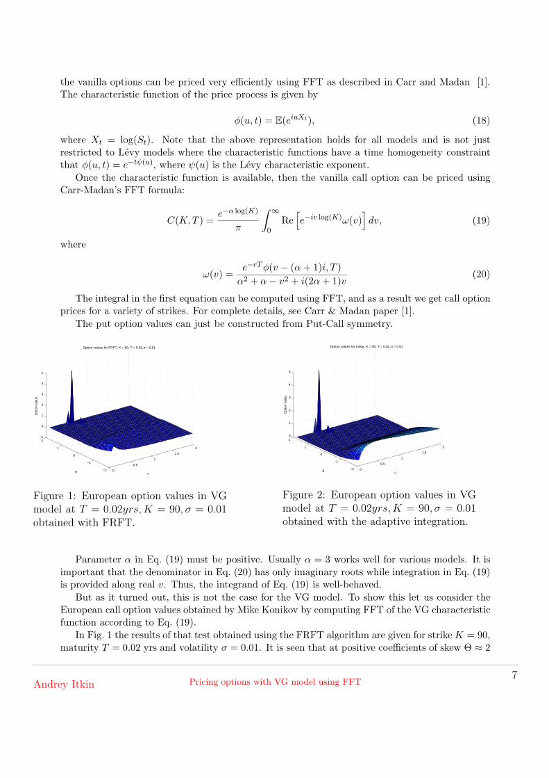
Parameter α in Eq. (19) must be positive. Usually α = 3 works well for various models. It isimportant that the denominator in Eq. (20) has only imaginary roots while integration in Eq. (19)is provided along real v. Thus, the integrand of Eq. (19) is well-behaved.

But as it turned out, this is not the case for the VG model. To show this let us consider theEuropean call option values obtained by Mike Konikov by computing FFT of the VG characteristicfunction according to Eq. (19).

In Fig. 1 the results of that test obtained using the FRFT algorithm are given for strike K = 90,maturity T = 0.02 yrs and volatility σ = 0.01. It is seen that at positive coefficients of skew Θ ≈ 2


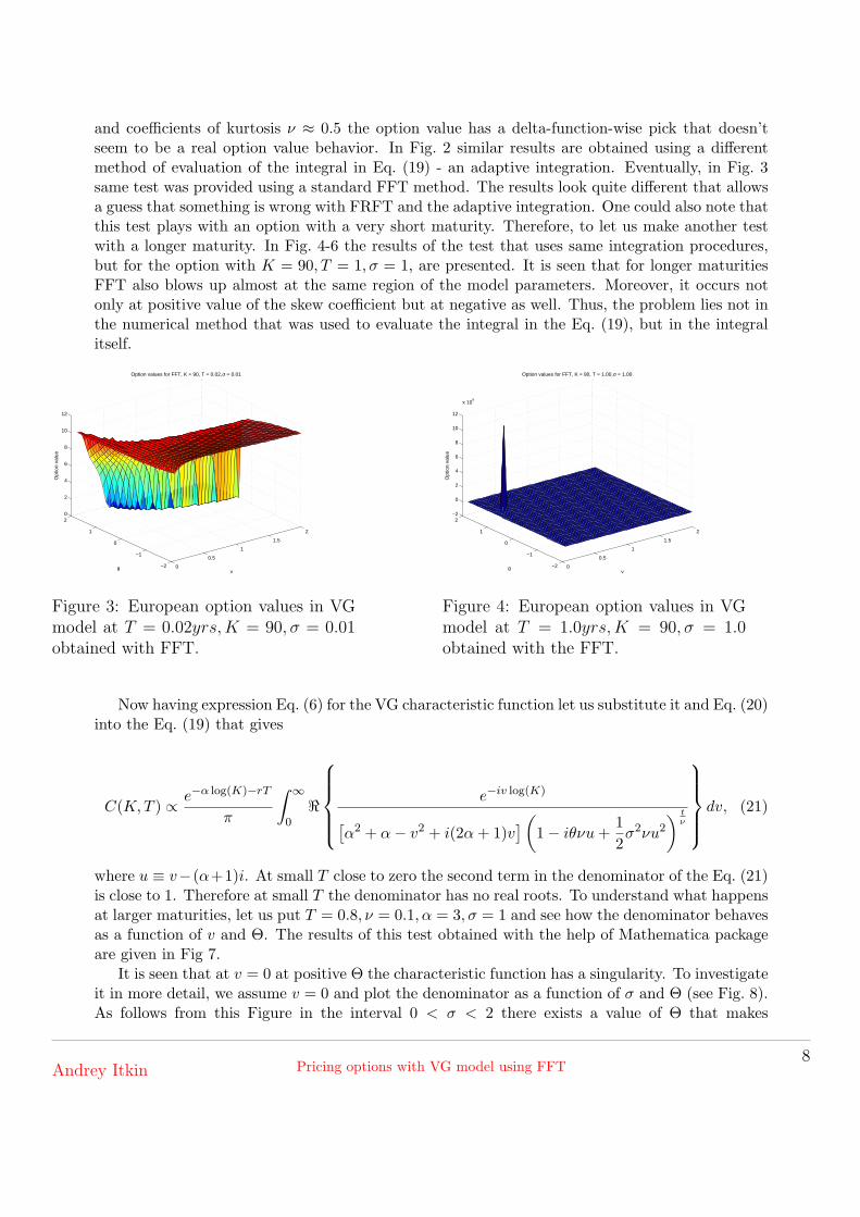
and coefficients of kurtosis ν ≈ 0.5 the option value has a delta-function-wise pick that doesn’tseem to be a real option value behavior. In Fig. 2 similar results are obtained using a differentmethod of evaluation of the integral in Eq. (19) - an adaptive integration. Eventually, in Fig. 3same test was provided using a standard FFT method. The results look quite different that allowsa guess that something is wrong with FRFT and the adaptive integration. One could also note thatthis test plays with an option with a very short maturity. Therefore, to let us make another testwith a longer maturity. In Fig. 4-6 the results of the test that uses same integration procedures,but for the option with K = 90, T = 1, σ = 1, are presented. It is seen that for longer maturitiesFFT also blows up almost at the same region of the model parameters. Moreover, it occurs notonly at positive value of the skew coefficient but at negative as well. Thus, the problem lies not inthe numerical method that was used to evaluate the integral in the Eq. (19), but in the integralitself.

0

0.5

1

1.5

2

−2

−1

0

1

20

2

4

6

8

10

12

ν

Option values for FFT, K = 90, T = 0.02, σ = 0.01

θ

Opt

ion

valu

e

Figure 3: European option values in VGmodel at T = 0.02yrs, K = 90, σ = 0.01obtained with FFT.

0

0.5

1

1.5

2

−2

−1

0

1

2−2

0

2

4

6

8

10

12

x 109

ν

Option values for FFT, K = 90, T = 1.00, σ = 1.00

θ

Opt

ion

valu

e

Figure 4: European option values in VGmodel at T = 1.0yrs, K = 90, σ = 1.0obtained with the FFT.

Now having expression Eq. (6) for the VG characteristic function let us substitute it and Eq. (20)into the Eq. (19) that gives

C(K, T ) ∝ e−α log(K)−rT

π

∫ ∞

0<

e−iv log(K)

[α2 + α− v2 + i(2α + 1)v

](1− iθνu +

12σ2νu2

) tν

dv, (21)

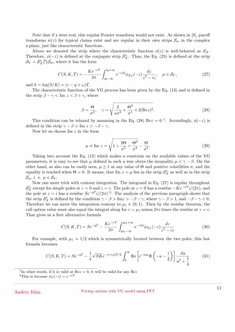
where u ≡ v−(α+1)i. At small T close to zero the second term in the denominator of the Eq. (21)is close to 1. Therefore at small T the denominator has no real roots. To understand what happensat larger maturities, let us put T = 0.8, ν = 0.1, α = 3, σ = 1 and see how the denominator behavesas a function of v and Θ. The results of this test obtained with the help of Mathematica packageare given in Fig 7.

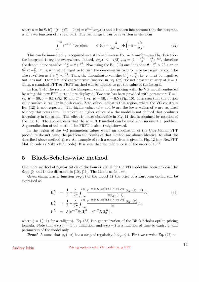
It is seen that at v = 0 at positive Θ the characteristic function has a singularity. To investigateit in more detail, we assume v = 0 and plot the denominator as a function of σ and Θ (see Fig. 8).As follows from this Figure in the interval 0 < σ < 2 there exists a value of Θ that makes


0

0.5

1

1.5

2

−2

−1

0

1

2−1

0

1

2

3

4

5

6

7

x 109

ν

Option values for FRFT, K = 90, T = 1.00, σ = 1.00

θ

Opt

ion

valu

e

Figure 5: European option values in VGmodel at T = 1.0yrs, K = 90, σ = 1.0obtained with the FRFT.

0

0.5

1

1.5

2

−2

−1

0

1

20

10

20

30

40

50

60

70

80

90

ν

Option values for Integr, K = 90, T = 1.00, σ = 1.00

θ

Opt

ion

valu

e

Figure 6: European option values in VGmodel at T = 1.0yrs, K = 90, σ = 1.0obtained with the adaptive integration.

the integrand in the Eq. (21) singular. This means that singularity of the integrand can not beeliminated, and thus the Carr-Madan FFT method can not be used together with the VG modelfor pricing European vanilla options. Using FRFT or adaptive integration that both are slightmodifications of the FFT, also doesn’t help.

Note that for the VG model the authors of [1] derived condition which keeps the characteristicfunction to be finite, that reads

α <

√2

νσ2 +Θ2

σ4 −Θσ2 − 1. (22)

Figure 7: Denominator of the Eq. (21)at T = 0.8, ν = 0.1, α = 3, σ = 1 as afunction of v and Θ.

Figure 8: Denominator of the Eq. (21)at T = 0.8, ν = 0.1, α = 3, v = 0 as afunction of σ and Θ.

Also as can be seen, for Θ, ν and σ corresponding to the above mentioned tests α becomesnegative that doesn’t allow using this method to price the options in terms of strike.


In order to solve these problems one needs to find another way how to regularize the integrand,i.e. eliminate doing it in the way as Carr and Madan did it using a regularization factor e−αk.

4 Lewis’s regularization

Another approach of how to apply FFT to the pricing of European options was proposed by AlanLewis [7]. Lewis notes that a general integral representation of the European call option value witha vanilla payoff is

CT (x0,K) = e−rT

∫ ∞

−∞(ex −K)+ q(x, x0, T )dx, (23)

where x = log ST is a stock price that under a pricing measure evolves as ST = S0 exp[(r−q)T +XT ,r−q is the cost of carry, T is the expiration time for some option, XT is some Levy process satisfyingE[exp(iuXT )] = 1, and q is the density of the log-return distribution x.

The central point of the Lewis’s work is to represent the Eq. (23) as a convolution integral andthen apply a Parseval identity

∫ ∞

−∞f(x)g(x0 − x)dx =

12π

∫ ∞

−∞e−iux0 f(u)g(u)du, (24)

where the hat over function denotes its Fourier transform.The idea behind this formula is that the Fourier transform of a transition probability density

for a Levy process to reach Xt = x after the elapse of time t is a well-known characteristicfunction, which plays an important role in mathematical finance. For Levy processes it is φt(u) =E[exp(iuXt)], u ∈ <, and typically has an analytic extension (a generalized Fourier transform)u → z ∈ C, regular in some strip SX parallel to the real z-axis.

Now suppose that the generalized Fourier transform of the payoff function w(z) =∫∞−∞ eizx(ex−

K)+dx and the characteristic function φt(z) both exist (we will discuss this below). Then from achain of equalities the call option value can be expressed as follows

CT (x0,K) = e−rTE[(ex −K)+

]=

e−rT

2πE

[∫ iµ+∞

iµ−∞e−izxT w(z)dz

](25)

=e−rT

2πE

[∫ iµ+∞

iµ−∞e−iz[x0+(r−q+ω)T ]e−izXT w(z)dz

]

=e−rT

2π

∫ iµ+∞

iµ−∞e−iz[x0+(r−q+ω)T ]E[e−izXT ]w(z)dz =

e−rT

2π

∫ iµ+∞

iµ−∞e−izY φXT

(−z)w(z)dz.

Here Y = x0 +(r− q +ω)T , µ ≡ Im z. This is a formal derivation which becomes a valid proofif all the integrals in Eq. (25) exist.

The Fourier transform of the vanilla payoff can be easily found by a direct integration

w(z) =∫ ∞

−∞eizx(ex −K)+dx = − Kiz+1

z2 − iz, Imz > 1. (26)


Note that if z were real, this regular Fourier transform would not exist. As shown in [8], payofftransforms w(z) for typical claims exist and are regular in their own strips Sw in the complexz-plane, just like characteristic functions.

Above we denoted the strip where the characteristic function φ(z) is well-behaved as SX .Therefore, φ(−z) is defined at the conjugate strip S∗X . Thus, the Eq. (25) is defined at the stripSV = S∗X

⋂Sw, where it has the form

C(S, K, T ) = −Ke−rT

2π

∫ iµ+∞

iµ−∞e−izkφXT

(−z)dz

z2 − iz, µ ∈ SV , (27)

and k = log(S/K) + (r − q + ω)T .The characteristic function of the VG process has been given by the Eq. (13) and is defined in

the strip β − γ < Im z < β + γ, where

β =Θσ2 , γ =

√2

νσ2 +Θ2

σ4 + 2(Rez)2. (28)

This condition can be relaxed by assuming in the Eq. (28) Rez = 0 1. Accordingly, φ(−z) isdefined in the strip γ − β > Im z > −β − γ.

Now let us choose Im z in the form

µ ≡ Im z =

√1 +

2Θσ2 +

Θ2

σ4 −Θσ2 . (29)

Taking into account the Eq. (12) which makes a constrain on the available values of the VGparameters, it is easy to see that µ defined in such a way obeys the inequality µ < γ − β. On theother hand, as also can be easily seen, µ ≥ 1 at any value of Θ and positive volatilities σ, and theequality is reached when Θ = 0. It means, that Im z = µ lies in the strip S∗X as well as in the stripSw, i. e. µ ∈ SV .

Now one more trick with contour integration. The integrand in Eq. (27) is regular throughoutS∗X except for simple poles at z = 0 and z = i. The pole at z = 0 has a residue −Ke−rT i/(2π), andthe pole at z = i has a residue Se−qT i/(2π) 2. The analysis of the previous paragraph shows thatthe strip S∗X is defined by the condition γ − β > Imz > −β − γ, where γ − β > 1, and −β − γ < 0.Therefore we can move the integration contour to µ1 ∈ (0, 1). Then by the residue theorem, thecall option value must also equal the integral along Im z = µ1 minus 2πi times the residue at z = i.That gives us a first alternative formula

C(S,K, T ) = Se−qT − Ke−rT

2π

∫ iµ1+∞

iµ1−∞e−izkφXT

(−z)dz

z2 − iz(30)

For example, with µ1 = 1/2 which is symmetrically located between the two poles, this lastformula becomes

C(S,K, T ) = Se−qT − 1π

√SKe−(r+q)T/2

∫ ∞

0Re

[e−iuκΦ

(−u− i

2

)]du

u2 +14

(31)

1In other words, if it is valid at Rez = 0, it will be valid for any Rez2This is because φT (−i) = e−ωT


where κ = ln(S/K)+(r−q)T, Φ(u) = eiuωT φXT(u) and it is taken into account that the integrand

is an even function of its real part. The last integral can be rewritten in the form

∫ ∞

0e−iu ln κφ1(u)du, φ1(u) =

44u2 + 1

Φ(−u− i

2

). (32)

This can be immediately recognized as a standard inverse Fourier transform, and by derivationthe integrand is regular everywhere. Indeed, φXT

(−u − i/2)|u=0 = (1 − σ2ν8 − νθ

2 )−t/ν , thereforethe denominator vanishes if 2

ν = θ + σ2

4 . Now using the Eq. (12) one finds that θ + σ2

4 > 2h+σ2 orσ2

4 < − θ3 . Thus, θ must be negative to turn the denominator to zero. The last equality could be

also rewritten as θ + σ2

4 < 2θ3 . Thus, the denominator vanishes if 1

ν < 2θ3 , i.e. ν must be negative,

but it is not! Therefore, the characteristic function in Eq. (32) doesn’t have singularity at u = 0.Thus, a standard FFT or FRFT method can be applied to get the value of the integral.

In Fig. 9 -10 the results of the European vanilla option pricing with the VG model conductedby using this new FFT method are displayed. Two test has been provided with parameters T = 1yr, K = 90, σ = 0.1 (Fig. 9) and T = 1 yr, K = 90, σ = 0.5 (Fig. 10). It is seen that the optionvalue surface is regular in both cases. Zero values indicates that region, where the VG constrainEq. (12) is not respected. The higher values of σ and Θ are the lower values of ν are requiredto obey this constraint. Therefore, at higher values of ν the model is not defined that producesirregularity in the graph. This effect is better observable in Fig. 11 that is obtained by rotation ofthe Fig. 10. The above means that the new FFT method can be used with no essential problem.A generalization of this method for FRFT is also straightforward.

In the region of the VG parameters values where an application of the Carr-Madan FFTprocedure doesn’t cause the problem the results of that method are almost identical to what thedescribed above method gives. An example of such a comparison is given in Fig. 12 (my NewFFTMatlab code vs Mike’s FFT code). It is seen that the difference is of the order of 10−7.

5 Black-Scholes-wise method

One more method of regularization of the Fourier kernel for the VG model has been proposed bySepp [9] and is also discussed in [10], [11]. The idea is as follows.

Given characteristic function φXt(z) of the model M the price of a European option can beexpressed as

ΠM1 =

12

+ξ

2π

∫ ∞

−∞

e−iu ln Keiu[ln S+(r−q+ω)T ]φXT(u− i)

iuφXT(−i)

du, (33)

ΠM2 =

12

+ξ

2π

∫ ∞

−∞

e−iu ln Keiu[ln S+(r−q+ω)T ]φXT(u)

iudu,

V M = ξ[e−qT S0ΠM

1 − e−rT KΠM2

],

where ξ = 1(−1) for a call(put). Eq. (33) is a generalization of the Black-Scholes option pricingformula. Note that φXt(0) = 1 by definition, and φXt(−i) is a function of time to expiry T andparameters of the model only.

Proof: Assume that φT (−z) has a strip of regularity 0 ≤ µ ≤ 1. First we rewrite Eq. (27) as


0

0.1

0.2

0.3

0.4

0.5

−3

−2

−1

0

1

20

20

40

60

80

100

Nu

Call Option Value − VG model with a new FFT

Theta

C(T

,S,K

)

Figure 9: European option values in VGmodel at T = 1.0yr,K = 90, σ = 0.1obtained with the new FFT method.

0

0.2

0.4

0.6

0.8

1

−3

−2

−1

0

1

20

20

40

60

80

100

Nu


Theta

C(T

,S,K

)

Figure 10: European option values in VGmodel at T = 1.0yrs, K = 90, σ = 0.5obtained with the new FFT method.

0

0.2

0.4

0.6

0.8

1

−3−2

−10

12

0

20

40

60

80

100

Theta


Nu

C(T

,S,K

)

Figure 11: European option values in VG model at T = 1.0yr,K = 90, σ = 0.5 obtained with the newFFT method (rotated graph).

C(S, K, T ) = −Ke−rT

2π

∫ iµ+∞


(−z)dz

z2 − iz(34)

= −Ke−rT

2π

[∫ iµ+∞


(−z)idz

z−

∫ iµ+∞


(−z)idz

z − i

]

= −Ke−rT

2π(R(I1)−R(I2))

In order to evaluate I1 we employ a contour integral over the contour given by 6 parametriccurves (see Fig. (13): Γ1 : z = u, u ∈ (q,R), q, R > 0; Γ2 : z = R + ib, b ∈ (0, v); Γ3 : z = u + iv, u ∈(R,−R); Γ4 : z = −R + ib, b ∈ (v, 0); Γ5 : z = u, u ∈ (−R,−q); Γ6 : z = qeiθ, θ ∈ (π, 0). As theintegrand is analytic on this contour we can apply the Cauchy theorem. Also note that the integralalong curve Γ6 is a half of the integral along the whole circle around zero which in turn is equalto 2πi2Res(e−izkφt(−z)/z). As the integrals along vertical lines vanish at R → ∞ and at q → 0


80 85 90 95 100 105 110 115 120−2

0

2

4

6

8

10

12

14x 10

−7

Strike

Opt

ion

Cal option value for vgCharFn model

Figure 12: The difference between the European call option values for the VG model obtained withCarr-Madan FFT method and the new FFT method. Parameters of the test are: S = 100, T =0.5yr, σ = 0.2, ν = 0.1, Θ = −0.33, r = q = 0. at various strikes).

Figure 13: Integration contour for R(I1).

the integral along the real axis tends to an integral from −∞ to ∞, eventually changing variableu → −u we obtain

R(I1) = π +∫ ∞

−∞e−iu ln Keiu[ln S+(r−q+ω)T ] φXT

(u)iu

du. (35)

To compute the R(I2) we use a similar contour build around the point z = i, i.e. Γ1 : z =u + i, u ∈ (q,R), q, R > 0; Γ2 : z = R + ib, b ∈ (1, 1 + v); Γ3 : z = u + i(1 + v), u ∈ (R,−R); Γ4 : z =−R + ib, b ∈ (v, 1); Γ5 : z = u + i, u ∈ (−R,−q); Γ6 : z = i + qeiθ, θ ∈ (0, π). Again taking limitsR →∞ and q → 0, changing variable u → u− i, we obtain

R(I2) =S

Ke(r−q)T

(π +

∫ ∞

−∞e−iu ln Keiu[ln S+(r−q+ω)T ] φXT

(u− i)iuφXT

(−i)du

). (36)

Substituting these integrals into the Eq. (34) we obtain the Eq. (33) ¥.The difficulty in using FFT to evaluate the Eqs. (33), as noted by Carr and Madan is the

divergence of the integrands at u = 0. Specifically, let us develop the characteristic functionφXt(z) with z = u + iv as Taylor series in u


φXt(z) = E[e−vXt ] + iuE[xe−vXt ]− 12u2E[x2e−vXt ] + ... (37)

In Eq. (30) we have to chose z = u − i in the first expression, and z = u in the second one.As it is easy to check in both cases that the leading term in the expansion under both integralsis 1/(iu) which is just a source of the divergence.The source of this divergence is a discontinuityof the payoff function at K = ST . Accordingly the Fourier transform of the payoff function haslarge high-frequency terms. The Carr-Madan solution is in fact to dampen the weight of thehigh frequencies by multiplying the payoff by an exponential decay function. This will lower theimportance of the singularity, but at the cost of degradation of the solution accuracy.

As the Eqs. (33) can be used whenever the characteristic function of the given model is known,we can apply it to the Black-Scholes model as well that gives us the Black-Scholes option priceV BS which is a well known analytic expression. Now the idea is to rewrite representation of theoption price in the Eqs. (33) in the form

V M = [V M − V BS ] + V BS . (38)

The term in braces can now be computed with FFT as

ΠM−BS1 =

ξ

2π

∫ ∞

−∞

e−iuκ

[φXt(u− i)ei(u−i)ωT − φBS(u− i)e−

σ2

2T

]

iudu, (39)

ΠM−BS2 =

ξ

2π

∫ ∞

−∞

e−iuκ[φXt(u)eiuωT − φBS(u)

]

iudu,

V M − V BS = ξ[e−qT S0ΠM−BS

1 − e−rT KΠM−BS2

],

where κ = ln(K/S) − (r − q)T , φBS(u) = exp(−σ2T

2 u2)

and φXT(−i) = e−ωT . This is possible

because we have removed the divergence in the integrals. In addition the magnitude of φXt(z) −φBS(z) is smaller than that of φXt(z) that increases accuracy of the solution.

In more detail, first terms of the expansion of φXt(u)eiuωT − φBS(u) and φXt(u− i)ei(u−i)ωT −φBS(u− i)e−

σ2

2T in series at small u are

D1|u=0 ≡ φXt(u)eiuωT − φBS(u) = T (θ + ω +σ2

2)iu + O(u2) (40)

D2|u=0 ≡ φXt(u− i)ei(u−i)ωT − φBS(u− i)e−σ2

2T = −

(σ2 +

θ + σ2

−1 + ν(θ + σ2/2)− ω

)iu + O(u2)

However, an usage of these expressions in the Eq. (39) together with the FFT method producesan error of the order of O(u). That is why it is better to choose a small u = ε, for instance ε = 10−6,then computing integrands in the Eq. (39) exactly and substituting D1,2|u=0 ≈ D1,2|u=ε.

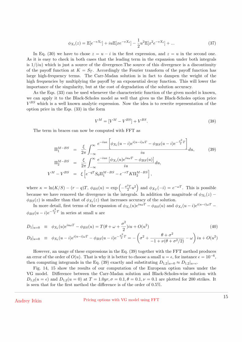
Fig. 14, 15 show the results of our computation of the European option values under theVG model. Difference between the Carr-Madan solution and Black-Scholes-wise solution withD1,2(u = ε) and D1,2(u = 0) at T = 1.0yr, σ = 0.1, θ = 0.1, ν = 0.1 are plotted for 200 strikes. Itis seen that for the first method the difference is of the order of 0.5%.


0 50 100 150 2000

0.005

0.01

0.015

0.02

0.025

K

CC

M −

CB

S, $

Difference between VG prices. "Carr−Madan" − "BS−wise"

Figure 14: European option values inVG model. Difference between the Carr-Madan solution and Black-Scholes-wisesolution with D1,2(u = 0) at T =1.0yr, σ = 0.1, θ = 0.1, ν = 0.1

0 50 100 150 200−5

−4

−3

−2

−1

0

1x 10

−3

K

CC

M −

CB

S, $

Difference between VG prices. "Carr−Madan" − "BS−wise"

Figure 15: European option values inVG model. Difference between the Carr-Madan solution and Black-Scholes-wisesolution with D1,2(u = ε) at T =1.0yr, σ = 0.1, θ = 0.1, ν = 0.1

6 Convergency and performance

Artur Sepp reported in [9] that the convergency of the Black-Scholes-wise method is approximately3 times faster than that of the Lewis method. It could be understood because as we mentionedabove in the limit of small u the difference between the VG solution and the Black-Scholes formulawhich is under the Fourier integral is of the second order in u while in the Lewis method it is of thezero order. In other words using the Black-Scholes-wise formula allows us to remove a part of theFFT error instead substituting it with the exact analytical solution of the Black-Scholes problem.

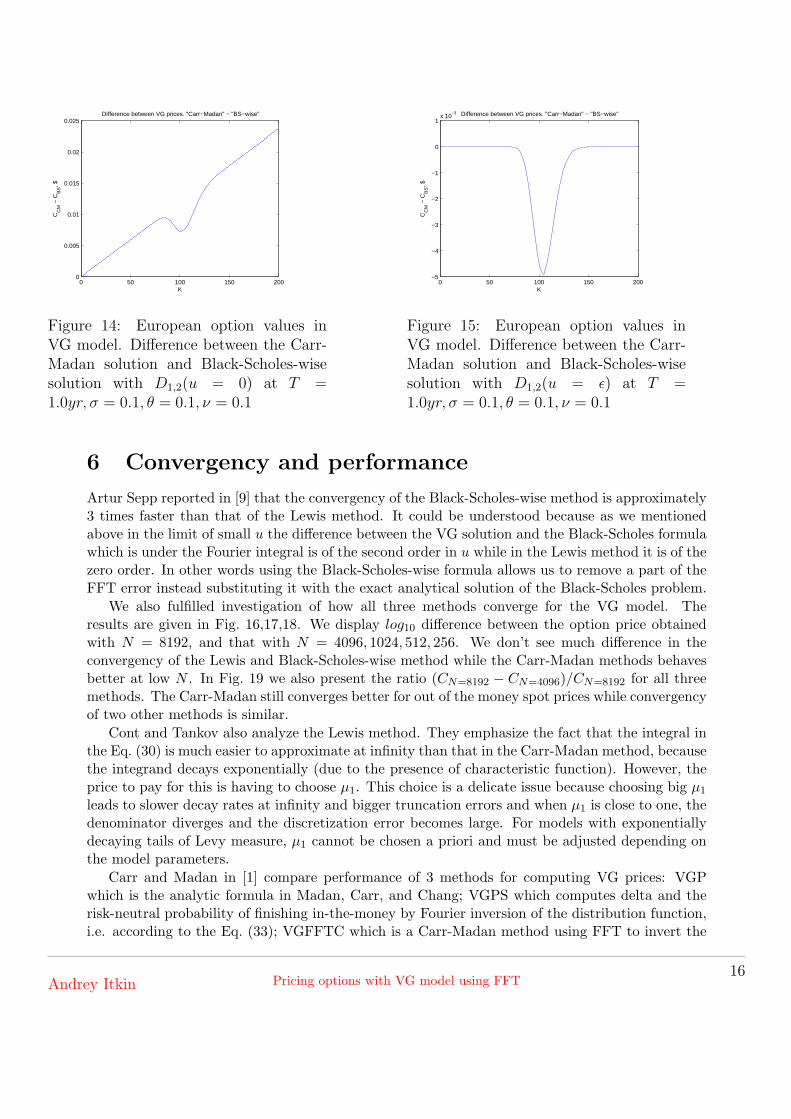
We also fulfilled investigation of how all three methods converge for the VG model. Theresults are given in Fig. 16,17,18. We display log10 difference between the option price obtainedwith N = 8192, and that with N = 4096, 1024, 512, 256. We don’t see much difference in theconvergency of the Lewis and Black-Scholes-wise method while the Carr-Madan methods behavesbetter at low N . In Fig. 19 we also present the ratio (CN=8192 − CN=4096)/CN=8192 for all threemethods. The Carr-Madan still converges better for out of the money spot prices while convergencyof two other methods is similar.

Cont and Tankov also analyze the Lewis method. They emphasize the fact that the integral inthe Eq. (30) is much easier to approximate at infinity than that in the Carr-Madan method, becausethe integrand decays exponentially (due to the presence of characteristic function). However, theprice to pay for this is having to choose µ1. This choice is a delicate issue because choosing big µ1

leads to slower decay rates at infinity and bigger truncation errors and when µ1 is close to one, thedenominator diverges and the discretization error becomes large. For models with exponentiallydecaying tails of Levy measure, µ1 cannot be chosen a priori and must be adjusted depending onthe model parameters.

Carr and Madan in [1] compare performance of 3 methods for computing VG prices: VGPwhich is the analytic formula in Madan, Carr, and Chang; VGPS which computes delta and therisk-neutral probability of finishing in-the-money by Fourier inversion of the distribution function,i.e. according to the Eq. (33); VGFFTC which is a Carr-Madan method using FFT to invert the


0 50 100 150 200−15

−10

−5

0

K

Log(

C81

92 −

CN

)

Convergency of the Black−Scholes−wise method for VG model

N=4096N=2048N=1024N=512N=256

Figure 16: Convergency of the Black-Scholes-wise method. Difference betweenthe option price obtained with N = 8192,and that with N = 4096, 1024, 512, 256.

0 50 100 150 200−14

−12

−10

−8

−6

−4

−2

0

K

Log(

C81

92 −

CN

)

Convergency of the Lewis method for VG model

N=4096N=2048N=1024N=512N=256

Figure 17: Convergency of the Lewismethod. Difference between the optionprice obtained with N = 8192, and thatwith N = 4096, 1024, 512, 256.

dampened call price; VGFFTTV which uses FFT to invert the modified time value. The resultsare given in Tab. (1). The computation times for the first two methods involve 160 strike levels.The first 4 rows of Tab. (1) display 4 combinations of parameter settings, while the last 4 rowsshow computation times in seconds.

case 1 case 2 case 3 case 4σ .12 .25 .12 .25ν .16 2.0 .16 2.0θ -.33 -.10 -.33 -.10T 1 1 .25 .25VGP 22.41 24.81 23.82 24.74VGPS 288.50 191.06 181.62 197.97VGFFTC 6.09 6.48 6.72 6.52VGFFTTV 11.53 11.48 11.57 11.56

Table 1: CPU times for VG pricing. Rep-resented from [1].

case 1 case 2 case 3 case 4σ .12 .25 .12 .25ν .16 2.0 .16 2.0θ -.33 -.10 -.33 -.10T 1 1 .25 .25Lewis 0.031 0.031 0.031 0.031Carr-Madan 0.047 0.047 0.032 0.032BS-wise 0.078 0.078 0.062 0.062

Table 2: CPU times for VG pricing. Ourcalculations.

It is seen that the analytic formula is slow while the slowest (and least accurate in case 4)method inverts for the delta and for the probability of paying off.

However, this is not true if one uses a modified method given in the Eq. (39). Our calculationsshow that the performance of the Lewis method is same as the Carr-Madan method, and theperformance of the Black-Scholes-wise method is only twice worse (because we need 2 FFT tocompute 2 integrals) (see Tab. 2).


0 50 100 150 200−15

−10

−5

0

K

Log(

C81

92 −

CN

)

Convergency of the Carr−Madan method for VG model

N=4096N=2048N=1024N=512N=256

Figure 18: Convergency of the Carr-Madan method. Difference between theoption price obtained with N = 8192, andthat with N = 4096, 1024, 512, 256.

0 50 100 150 200−3

−2.5

−2

−1.5

−1

−0.5

0

0.5

1x 10

−5

K

(C81

92 −

C40

96)/

C81

92

Convergency of three methods for VG model

BSLewisCM

Figure 19: Convergency of all three meth-ods.

7 Conclusion

We discussed various analytic and numerical methods that have been used to get option priceswithin a framework of VG model. We showed that a popular Carr-Madan’s FFT method [1]blows up for certain values of the model parameters even for European vanilla option. Alternativemethods - one originally proposed by Lewis, and Black-Scholes-wise method were considered thatseem to work fine for any value of the VG parameters. Convergency and accuracy of these methodsis comparable with that of the Carr-Madan method, thus making them suitable for being used toprice options with the VG model.


References

[1] Peter Carr and Dilip Madan. Option valuation using the fast fourier transform. Journal ofComputational Finance, 2(4):61–73, 1999.

[2] D. Madan and E. Seneta. The variance gamma (v.g.) model for share market returns. Journalof Business, 63(4):511–524, 1990.

[3] D. Madan, P. Carr, and E. Chang. The variance gamma process and option pricing. EuropeanFinance Review, 2:79–105, 1998.

[4] D. Madan and M. Konikov. Variance gamma model: Gamma weighted black-scholes imple-mentation. Technical report, Bloomberg L.P., 2004.

[5] D. H. Bailey and P.N. Swarztrauber. The fractional fourier transform and applications. SIAMReview, 33(3):389–404, 1991.

[6] K. Chourdakis. Option pricing using the fractional fft. Technical report, 2004.

[7] Alan L. Lewis. A simple option formula for general jump-diffusion and other exponentiallevy processes. manuscript, Envision Financial Systems and OptionCity.net, Newport Beach,California, USA, 2001.

[8] Alan L. Lewis. Option Valuation under Stochastic Volatility. Finance Press, Newport Beach,California, USA, 2000.

[9] A. Sepp. Fourier transform for option pricing under affine-jump-diffusions: An overview.Unpublished Manuscript, available at www.hot.ee/seppar, 2003.

[10] I. Yekutieli. Pricing european options with fft. Technical report, Bloomberg L.P., November2004.

[11] R. Cont and P. Tankov. Financial modelling with jump processes. Chapman & Hall / CRC,2004.


Documents

Pricing options with VG model using FFT - UCLAitkin/publications/virginia2005.pdf · 2 Pricing European option 6 3 Carr-Madan’s FFT approach and the VG model 6 ... investigate various