Embed Size (px)
Citation preview

Pricing options with VG model using FFT
Andrey Itkin
Moscow State Aviation University
Department of applied mathematics and physics
A.Itkin ”Pricing options with VG model using FFT”. The Variance Gamma and Related Financial Models. August 9, 2007 – p. 1/40

The idea of the work
Discuss various analytic and numerical methods that have
been used to price options within a framework of the VG
model
A.Itkin ”Pricing options with VG model using FFT”. The Variance Gamma and Related Financial Models. August 9, 2007 – p. 2/40

The idea of the work
Discuss various analytic and numerical methods that have
been used to price options within a framework of the VG
model
Show that some popular methods, for instance,
Carr-Madan’s FFT method could blow up at certain values of
the model parameters even for an European vanilla option
A.Itkin ”Pricing options with VG model using FFT”. The Variance Gamma and Related Financial Models. August 9, 2007 – p. 2/40
The idea of the work
Discuss various analytic and numerical methods that have
been used to price options within a framework of the VG
model
Show that some popular methods, for instance,
Carr-Madan’s FFT method could blow up at certain values of
the model parameters even for an European vanilla option
Consider alternative methods - Lewis-wise and
Black-Scholes-wise and show that they seem to work fine for
any value of the VG parameters
A.Itkin ”Pricing options with VG model using FFT”. The Variance Gamma and Related Financial Models. August 9, 2007 – p. 2/40

The idea of the work
Discuss various analytic and numerical methods that have
been used to price options within a framework of the VG
model
Show that some popular methods, for instance,
Carr-Madan’s FFT method could blow up at certain values of
the model parameters even for an European vanilla option
Consider alternative methods - Lewis-wise and
Black-Scholes-wise and show that they seem to work fine for
any value of the VG parameters
Give test examples to demonstrate efficiency of these
methods and discuss convergency and accuracy of all
methods
A.Itkin ”Pricing options with VG model using FFT”. The Variance Gamma and Related Financial Models. August 9, 2007 – p. 2/40

Brief overview of the VG model
A.Itkin ”Pricing options with VG model using FFT”. The Variance Gamma and Related Financial Models. August 9, 2007 – p. 3/40

VG model
Proposed by Madan and Seneta (1990) to describe stock
price dynamics instead of the Brownian motion in the original
Black-Scholes model.
Two new parameters: θ skewness and ν kurtosis are
introduced in order to describe asymmetry and fat tails of
real life distributions.
The VG process is defined by evaluating Brownian motion
with drift at a random time specified by gamma process.
lnFt = lnF0 + Xt + ωt, (2)
where
Xt = θγt(1, ν) + σWγt(1,ν), (3)
A.Itkin ”Pricing options with VG model using FFT”. The Variance Gamma and Related Financial Models. August 9, 2007 – p. 4/40

VG model (continue)
and γt(1, ν) is a Gamma process playing the role of time in this
case with unit mean rate and density function given by
fγt(1,ν)(x) =x
tν−1e−
xν
νtν Γ(
tν
) . (4)
The probability density function for the VG process may be written as
ht(x) =
∫
∞
0
dg√
2πgexp
[
− (x − θg)2
2σ2g
]
gtν−1e−
g
ν
νtν Γ(
tν
) (5)
or after integration over g
ht(x) =2eθx/σ2
√2πσν
tν Γ(t/ν)
(
x2
θ2 + 2σ2
ν
)t2ν
−14
K tν−
12
(
1
σ2
√
x2
(
θ2 +2σ2
ν
)
)
,
(6)
A.Itkin ”Pricing options with VG model using FFT”. The Variance Gamma and Related Financial Models. August 9, 2007 – p. 5/40

VG model (continue)
where K is the modified Bessel function of the second kind. The
characteristic function φγt(1,ν)(u) for the VG process has a
remarkably simple form
φt(u) ≡⟨
Eiux⟩
≡∫
∞
0
ht(x)eiuxdx =1
(1 − iθνu +1
2σ2νu2)
tν
. (7)
Now, to prevent arbitrage, we need Ft be a martingale, and, since Ft is
already an independent increment process, all we need is
E[Ft] = F0, (8)
This tells us that
ω = − lnφXt(−i)
t= −− t
ν ln(
1 − θν − 12σ2ν
)
t=
1
νln
(
1 − θν − 1
2σ2ν
)
.
(9)
A.Itkin ”Pricing options with VG model using FFT”. The Variance Gamma and Related Financial Models. August 9, 2007 – p. 6/40
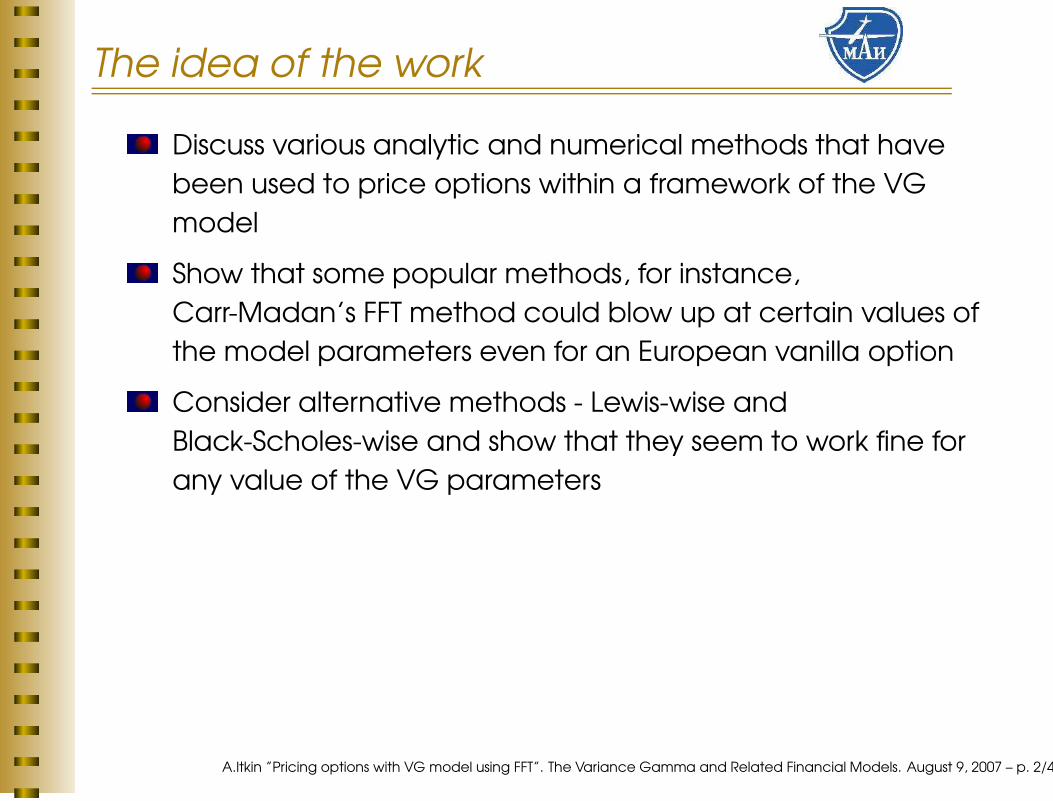
VG model (continue)
From the definition of ω above, in order to have a risk neutral
measure for VG model, its parameters must obey an inequality:
1
ν> θ +
σ2
2. (10)
Accordingly, the characteristic function of the xT ≡ log ST VG process is
φ(u) =
[
S0e(r−q+ω)T
]iu
(
1 − iθνu +1
2σ2νu2
)Tν
. (11)
A.Itkin ”Pricing options with VG model using FFT”. The Variance Gamma and Related Financial Models. August 9, 2007 – p. 7/40

VG model (continue)
Statistical parameters of VG distribution may be calculated
from the historical data on stock prices.
A.Itkin ”Pricing options with VG model using FFT”. The Variance Gamma and Related Financial Models. August 9, 2007 – p. 8/40

VG model (continue)
Statistical parameters of VG distribution may be calculated
from the historical data on stock prices.
In particular we have to find the values of the parameters
θ∗, ν∗ and σ∗ such that the follwing expression is maximized:
n∏
j=1
hτj(xj), (14)
where the PDF hτj(xj) were given above, and xj are observed
returns per time τj , i.e. xj = log(Sj/Sj−1).
A.Itkin ”Pricing options with VG model using FFT”. The Variance Gamma and Related Financial Models. August 9, 2007 – p. 8/40

VG model (continue)
Statistical parameters of VG distribution may be calculated
from the historical data on stock prices.
In particular we have to find the values of the parameters
θ∗, ν∗ and σ∗ such that the follwing expression is maximized:
n∏
j=1
hτj(xj), (15)
where the PDF hτj(xj) were given above, and xj are observed
returns per time τj , i.e. xj = log(Sj/Sj−1).
Note that risk neutral parameters θ, ν, σ do not have to be equal to
their statistical counterparts.
A.Itkin ”Pricing options with VG model using FFT”. The Variance Gamma and Related Financial Models. August 9, 2007 – p. 8/40

Pricing European option
A.Itkin ”Pricing options with VG model using FFT”. The Variance Gamma and Related Financial Models. August 9, 2007 – p. 9/40
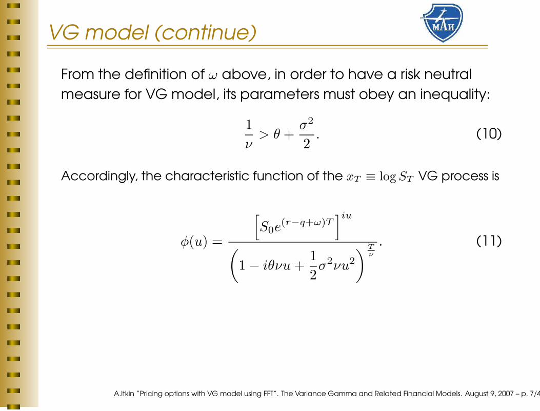
European option value
The value of European option on a stock when the risk neutral
dynamics is given by VG is
V = exp(−rT )
∫
∞
−∞
hT (x − (r − q + ω)T )W (ex)dx, (16)
where T is time until expiration, q is continuous dividend and W (ex) is
payoff function that has the following form
W (ex) = (S0ex − K)+ − call, W (ex) = (K − S0e
x)+ − put. (17)
Direct calculation allows us to derive the put-call parity relation
identical to Black-Scholes case
C = S0e−qT − Ke−rT + P. (18)
A.Itkin ”Pricing options with VG model using FFT”. The Variance Gamma and Related Financial Models. August 9, 2007 – p. 10/40

Existing methods of pricing
Closed form solution derived in D. Madan, P. Carr, and
E. Chang. ”The variance gamma process and option
pricing”. European Finance Review, 2:79–105, 1998. - slow
because it requires computation of modified Bessel
functions.
A.Itkin ”Pricing options with VG model using FFT”. The Variance Gamma and Related Financial Models. August 9, 2007 – p. 11/40

Existing methods of pricing
Closed form solution derived in D. Madan, P. Carr, and
E. Chang. ”The variance gamma process and option
pricing”. European Finance Review, 2:79–105, 1998. - slow
because it requires computation of modified Bessel
functions.
FFT methods. Carr and Madan method (1999) nowadays is
almost standard in math finance. Can be used since the VG
characteristic function has a very simple form given above.
Unfortunately this method blows up at some values of the VG
parameters as we will show below.
A.Itkin ”Pricing options with VG model using FFT”. The Variance Gamma and Related Financial Models. August 9, 2007 – p. 11/40

Existing methods of pricing
Closed form solution derived in D. Madan, P. Carr, and
E. Chang. ”The variance gamma process and option
pricing”. European Finance Review, 2:79–105, 1998. - slow
because it requires computation of modified Bessel
functions.
FFT methods. Carr and Madan method (1999) nowadays is
almost standard in math finance. Can be used since the VG
characteristic function has a very simple form given above.
Unfortunately this method blows up at some values of the VG
parameters as we will show below. FRFT!
Konikov and Madan in (”Variance gamma model: Gamma
weighted Black-Scholes implementation”, Technical report,
Bloomberg L.P., 2004) This method leads to a weighted sum of
the BS formulae while has not been implemented yet.
Monte-Carlo methods - slow.
A.Itkin ”Pricing options with VG model using FFT”. The Variance Gamma and Related Financial Models. August 9, 2007 – p. 11/40

Carr-Madan’s FFT approach and VG
Once the characteristic function φ(u, t) = E(eiuXt), where
Xt = log(St), is available, then the vanilla call option can be
priced using Carr-Madan’s FFT formula:
C(K, T ) =e−α log(K)
π
∫
∞
0
Re[
e−iv log(K)ω(v)]
dv, (19)
where
ω(v) =e−rT φ(v − (α + 1)i, T )
α2 + α − v2 + i(2α + 1)v(20)
The integral in the first equation can be computed using FFT, and as a
result we get call option prices for a variety of strikes. The put option
values can just be constructed from Put-Call parity.
Parameter α must be positive. Usually α = 3 works well for various
models. It is important that the denominator has only imaginary roots
while integration is provided along real v. Thus, the integrand ω(v) is
well-behaved.A.Itkin ”Pricing options with VG model using FFT”. The Variance Gamma and Related Financial Models. August 9, 2007 – p. 12/40

Carr-Madan’s FFT approach and VG
Once the characteristic function φ(u, t) = E(eiuXt), where
Xt = log(St), is available, then the vanilla call option can be
priced using Carr-Madan’s FFT formula:
C(K, T ) =e−α log(K)
π
∫
∞
0
Re[
e−iv log(K)ω(v)]
dv, (21)
where
ω(v) =e−rT φ(v − (α + 1)i, T )
α2 + α − v2 + i(2α + 1)v(22)
The integral in the first equation can be computed using FFT, and as a
result we get call option prices for a variety of strikes. The put option
values can just be constructed from Put-Call parity.
Parameter α must be positive. Usually α = 3 works well for various
models. It is important that the denominator has only imaginary roots
while integration is provided along real v. Thus, the integrand ω(v) is
well-behaved.A.Itkin ”Pricing options with VG model using FFT”. The Variance Gamma and Related Financial Models. August 9, 2007 – p. 12/40

Carr-Madan’s FFT approach and VG
Once the characteristic function φ(u, t) = E(eiuXt), where
Xt = log(St), is available, then the vanilla call option can be
priced using Carr-Madan’s FFT formula:
C(K, T ) =e−α log(K)
π
∫
∞
0
Re[
e−iv log(K)ω(v)]
dv, (23)
where
ω(v) =e−rT φ(v − (α + 1)i, T )
α2 + α − v2 + i(2α + 1)v(24)
The integral in the first equation can be computed using FFT, and as a
result we get call option prices for a variety of strikes. The put option
values can just be constructed from Put-Call parity.
Parameter α must be positive. Usually α = 3 works well for various
models. It is important that the denominator has only imaginary roots
while integration is provided along real v. Thus, the integrand ω(v) is
well-behaved.A.Itkin ”Pricing options with VG model using FFT”. The Variance Gamma and Related Financial Models. August 9, 2007 – p. 12/40

CM FFT results
0
0.5
1
1.5
2
−2
−1
0
1
2−1
0
1
2
3
4
5
ν
Option values for FRFT, K = 90, T = 0.02, σ = 0.01
θ
Opt
ion
valu
e
Figure 2: European option values
in VG model at T = 0.02yrs, K =
90, σ = 0.01 obtained with FRFT.
0
0.5
1
1.5
2
−2
−1
0
1
20
1
2
3
4
5
ν
Option values for Integr, K = 90, T = 0.02, σ = 0.01
θ
Opt
ion
valu
e
Figure 3: European option values
in VG model at T = 0.02yrs, K =
90, σ = 0.01 obtained with the
adaptive integration.
A.Itkin ”Pricing options with VG model using FFT”. The Variance Gamma and Related Financial Models. August 9, 2007 – p. 13/40

CM FFT results (continue)
0
0.5
1
1.5
2
−2
−1
0
1
20
2
4
6
8
10
12
ν
Option values for FFT, K = 90, T = 0.02, σ = 0.01
θ
Opt
ion
valu
e
Figure 4: European option values
in VG model at T = 0.02yrs, K =
90, σ = 0.01 obtained with FFT.
0
0.5
1
1.5
2
−2
−1
0
1
2−2
0
2
4
6
8
10
12
x 109
ν
Option values for FFT, K = 90, T = 1.00, σ = 1.00
θ
Opt
ion
valu
e
Figure 5: European option values
in VG model at T = 1.0yrs, K =
90, σ = 1.0 obtained with the FFT.
A.Itkin ”Pricing options with VG model using FFT”. The Variance Gamma and Related Financial Models. August 9, 2007 – p. 14/40

CM FFT results (continue)
0
0.5
1
1.5
2
−2
−1
0
1
2−1
0
1
2
3
4
5
6
7
x 109
ν
Option values for FRFT, K = 90, T = 1.00, σ = 1.00
θ
Opt
ion
valu
e
Figure 6: European option values
in VG model at T = 1.0yrs, K =
90, σ = 1.0 obtained with the FRFT.
0
0.5
1
1.5
2
−2
−1
0
1
20
10
20
30
40
50
60
70
80
90
ν
Option values for Integr, K = 90, T = 1.00, σ = 1.00
θ
Opt
ion
valu
e
Figure 7: European option values
in VG model at T = 1.0yrs, K =
90, σ = 1.0 obtained with the adap-
tive integration.
A.Itkin ”Pricing options with VG model using FFT”. The Variance Gamma and Related Financial Models. August 9, 2007 – p. 15/40

Investigation
European call option value in the Carr-Madan method
C(K, T ) ∝ e−α log(K)−rT
π
∫
∞
0
<(Ψ(v))dv (25)
Ψ(v) ≡ e−iv log(K)
[
α2 + α − v2 + i(2α + 1)v] (
1 − iθνu + σ2νu2/2)
tν
,
where u ≡ v − (α + 1)i. At small T the denominator has no real roots. To
understand what happens at larger maturities, let us put
T = 0.8, ν = 0.1, α = 3, σ = 1 and see how the denominator behaves as
a function of v and Θ.
A.Itkin ”Pricing options with VG model using FFT”. The Variance Gamma and Related Financial Models. August 9, 2007 – p. 16/40

Investigation
European call option value in the Carr-Madan method
C(K, T ) ∝ e−α log(K)−rT
π
∫
∞
0
<(Ψ(v))dv (27)
Ψ(v) ≡ e−iv log(K)
[
α2 + α − v2 + i(2α + 1)v] (
1 − iθνu + σ2νu2/2)
tν
,
where u ≡ v − (α + 1)i. At small T the denominator has no real roots. To
understand what happens at larger maturities, let us put
T = 0.8, ν = 0.1, α = 3, σ = 1 and see how the denominator behaves as
a function of v and Θ.
Carr and Madan’s condition to keep the characteristic function to be
finite
α <
√
2
νσ2 +Θ2
σ4 − Θ
σ2 − 1. (28)
A.Itkin ”Pricing options with VG model using FFT”. The Variance Gamma and Related Financial Models. August 9, 2007 – p. 16/40

Investigation (continue)
Figure 8: Denominator of Ψ(v) at
T = 0.8, ν = 0.1, α = 3, σ = 1 as a
function of v and Θ.
Figure 9: Denominator of Ψ(v) at
T = 0.8, ν = 0.1, α = 3, v = 0 as a
function of σ and Θ.
A.Itkin ”Pricing options with VG model using FFT”. The Variance Gamma and Related Financial Models. August 9, 2007 – p. 17/40

Lewis regularization
A.Itkin ”Pricing options with VG model using FFT”. The Variance Gamma and Related Financial Models. August 9, 2007 – p. 18/40

Lewis method
Alan Lewis (2001) notes that a general integral representation of
the European call option value with a vanilla payoff is
CT (x0, K) = e−rT
∫
∞
−∞
(ex − K)+
Q(x, x0, T )dx, (29)
where x = log ST is a stock price that under a pricing measure evolves
as ST = S0 exp[(r − q)T + XT ], and XT is some Levy process satisfying
E[exp(iuXT )] = 1, and Q is the density of the log-return distribution x.
The central point of the Lewis’s work is to represent this equation as a
convolution integral and then apply a Parseval identity
∫
∞
−∞
f(x)g(x0 − x)dx =1
2π
∫
∞
−∞
e−iux0 f(u)g(u)du, (30)
where the hat over function denotes its Fourier transform.
A.Itkin ”Pricing options with VG model using FFT”. The Variance Gamma and Related Financial Models. August 9, 2007 – p. 19/40

Lewis method (continue)
The idea behind this formula is that the Fourier transform of a transition
probability density for a Levy process to reach Xt = x after the elapse of
time t is a well-known characteristic function. For Levy processes it is
φt(u) = E[exp(iuXt)], u ∈ <, and typically has an analytic extension (a
generalized Fourier transform) u → z ∈ C, regular in some strip SX
parallel to the real z-axis.
A.Itkin ”Pricing options with VG model using FFT”. The Variance Gamma and Related Financial Models. August 9, 2007 – p. 20/40

Lewis method (continue)
The idea behind this formula is that the Fourier transform of a transition
probability density for a Levy process to reach Xt = x after the elapse of
time t is a well-known characteristic function. For Levy processes it is
φt(u) = E[exp(iuXt)], u ∈ <, and typically has an analytic extension (a
generalized Fourier transform) u → z ∈ C, regular in some strip SX
parallel to the real z-axis.
Suppose that the generalized Fourier transform of the payoff function
w(z) =R
∞
−∞eizx(ex − K)+dx and φt(z) both exist, the call option value is
CT (x0, K) = e−rTE
[
(ex − K)+]
=e−rT
2πE
[∫ iµ+∞
iµ−∞
e−izxT w(z)dz
]
=e−rT
2πE
[∫ iµ+∞
iµ−∞
e−iz[x0+(r−q+ω)T ]e−izXT w(z)dz
]
=e−rT
2π
∫ iµ+∞
iµ−∞
e−izY φXT(−z)w(z)dz.
Here Y = x0 + (r − q + ω)T , µ ≡ Im z. This is a formal derivation which
becomes a valid proof if all the integrals exist.
A.Itkin ”Pricing options with VG model using FFT”. The Variance Gamma and Related Financial Models. August 9, 2007 – p. 20/40

Lewis method (continue)
The Fourier transform of the vanilla payoff can be easily found by a
direct integration
w(z) =
∫
∞
−∞
eizx(ex − K)+dx = − Kiz+1
z2 − iz, Imz > 1. (33)
A.Itkin ”Pricing options with VG model using FFT”. The Variance Gamma and Related Financial Models. August 9, 2007 – p. 21/40

Lewis method (continue)
The Fourier transform of the vanilla payoff can be easily found by a
direct integration
w(z) =
∫
∞
−∞
eizx(ex − K)+dx = − Kiz+1
z2 − iz, Imz > 1. (35)
Note that if z were real, this regular Fourier transform would not exist. As
shown by Lewis, payoff transforms w(z) for typical claims exist and are
regular in their own strips Sw in the complex z-plane, just like
characteristic functions.
A.Itkin ”Pricing options with VG model using FFT”. The Variance Gamma and Related Financial Models. August 9, 2007 – p. 21/40
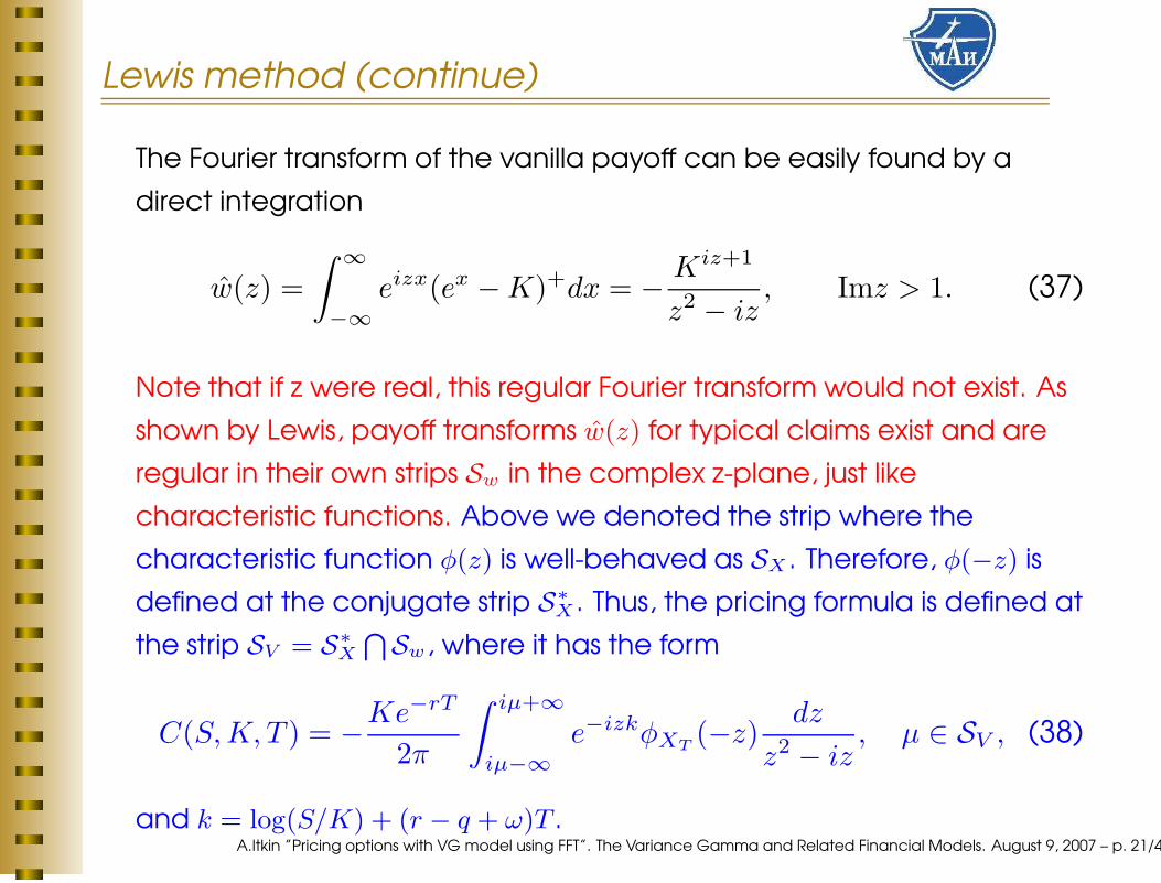
Lewis method (continue)
The Fourier transform of the vanilla payoff can be easily found by a
direct integration
w(z) =
∫
∞
−∞
eizx(ex − K)+dx = − Kiz+1
z2 − iz, Imz > 1. (37)
Note that if z were real, this regular Fourier transform would not exist. As
shown by Lewis, payoff transforms w(z) for typical claims exist and are
regular in their own strips Sw in the complex z-plane, just like
characteristic functions. Above we denoted the strip where the
characteristic function φ(z) is well-behaved as SX . Therefore, φ(−z) is
defined at the conjugate strip S∗
X . Thus, the pricing formula is defined at
the strip SV = S∗
X
T
Sw, where it has the form
C(S, K, T ) = −Ke−rT
2π
∫ iµ+∞
iµ−∞
e−izkφXT(−z)
dz
z2 − iz, µ ∈ SV , (38)
and k = log(S/K) + (r − q + ω)T .A.Itkin ”Pricing options with VG model using FFT”. The Variance Gamma and Related Financial Models. August 9, 2007 – p. 21/40

Lewis method (continue)
The Fourier transform of the vanilla payoff can be easily found by a
direct integration
w(z) =
∫
∞
−∞
eizx(ex − K)+dx = − Kiz+1
z2 − iz, Imz > 1. (39)
Note that if z were real, this regular Fourier transform would not exist. As
shown by Lewis, payoff transforms w(z) for typical claims exist and are
regular in their own strips Sw in the complex z-plane, just like
characteristic functions. Above we denoted the strip where the
characteristic function φ(z) is well-behaved as SX . Therefore, φ(−z) is
defined at the conjugate strip S∗
X . Thus, the pricing formula is defined at
the strip SV = S∗
X
T
Sw, where it has the form
C(S, K, T ) = −Ke−rT
2π
∫ iµ+∞
iµ−∞
e−izkφXT(−z)
dz
z2 − iz, µ ∈ SV , (40)
and k = log(S/K) + (r − q + ω)T .A.Itkin ”Pricing options with VG model using FFT”. The Variance Gamma and Related Financial Models. August 9, 2007 – p. 21/40
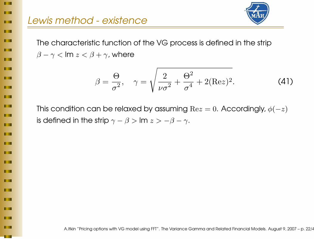
Lewis method - existence
The characteristic function of the VG process is defined in the strip
β − γ < Im z < β + γ, where
β =Θ
σ2 , γ =
√
2
νσ2 +Θ2
σ4 + 2(Rez)2. (41)
This condition can be relaxed by assuming Rez = 0. Accordingly, φ(−z)
is defined in the strip γ − β > Im z > −β − γ.
A.Itkin ”Pricing options with VG model using FFT”. The Variance Gamma and Related Financial Models. August 9, 2007 – p. 22/40

Lewis method - existence
The characteristic function of the VG process is defined in the strip
β − γ < Im z < β + γ, where
β =Θ
σ2 , γ =
√
2
νσ2 +Θ2
σ4 + 2(Rez)2. (43)
This condition can be relaxed by assuming Rez = 0. Accordingly, φ(−z)
is defined in the strip γ − β > Im z > −β − γ. Choose Im z in the form
µ ≡ Im z =
√
1 +2Θ
σ2 +Θ2
σ4 − Θ
σ2 . (44)
It is easy to see that µ defined in such a way obeys the inequality
µ < γ − β. On the other hand, µ ≥ 1 at any value of Θ and positive
volatilities σ, and the equality is reached when Θ = 0. It means, that Im
z = µ lies in the strip S∗
X as well as in the strip Sw, i. e. µ ∈ SV = S∗
X
T
Sw.
A.Itkin ”Pricing options with VG model using FFT”. The Variance Gamma and Related Financial Models. August 9, 2007 – p. 22/40
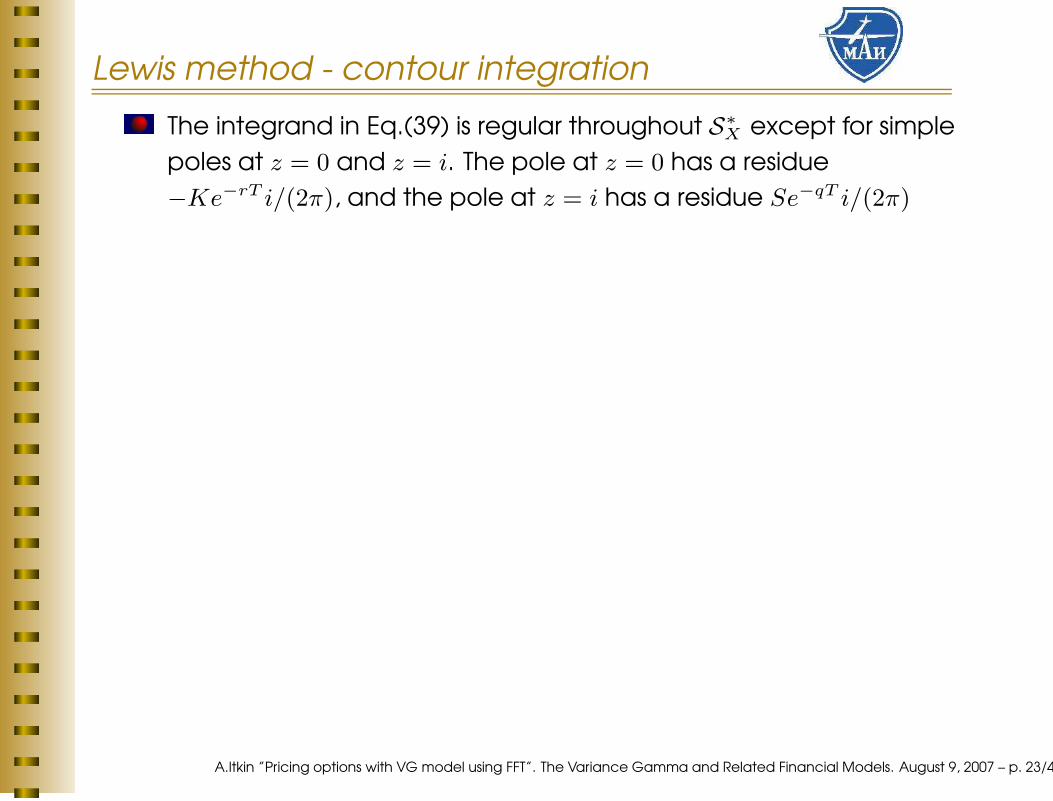
Lewis method - contour integration
The integrand in Eq.(39) is regular throughout S∗
X except for simple
poles at z = 0 and z = i. The pole at z = 0 has a residue
−Ke−rT i/(2π), and the pole at z = i has a residue Se−qT i/(2π)
A.Itkin ”Pricing options with VG model using FFT”. The Variance Gamma and Related Financial Models. August 9, 2007 – p. 23/40

Lewis method - contour integration
The integrand in Eq.(39) is regular throughout S∗
X except for simple
poles at z = 0 and z = i. The pole at z = 0 has a residue
−Ke−rT i/(2π), and the pole at z = i has a residue Se−qT i/(2π)
Strip S∗
X is defined by the condition γ − β > Imz > −β − γ, where
γ − β > 1, and −β − γ < 0. We can move the integration contour to
µ1 ∈ (0, 1) and use the residue theorem.
First alternative formula
C(S, K, T ) = Se−qT − Ke−rT
2π
∫ iµ1+∞
iµ1−∞
e−izkφXT(−z)
dz
z2 − iz(47)
A.Itkin ”Pricing options with VG model using FFT”. The Variance Gamma and Related Financial Models. August 9, 2007 – p. 23/40

Lewis method - contour integration
The integrand in Eq.(39) is regular throughout S∗
X except for simple
poles at z = 0 and z = i. The pole at z = 0 has a residue
−Ke−rT i/(2π), and the pole at z = i has a residue Se−qT i/(2π)
Strip S∗
X is defined by the condition γ − β > Imz > −β − γ, where
γ − β > 1, and −β − γ < 0. We can move the integration contour to
µ1 ∈ (0, 1) and use the residue theorem.
First alternative formula
C(S, K, T ) = Se−qT − Ke−rT
2π
∫ iµ1+∞
iµ1−∞
e−izkφXT(−z)
dz
z2 − iz(48)
Example: µ1 = 1/2
C(S, K, T ) = Se−qT −√
SK
πe−
(r+q)T
2
∫
∞
0
Re
[
e−iuκΦ
(
−u − i
2
)]
du
u2 + 1/4
where κ = ln(S/K) + (r − q)T, Φ(u) = eiuωT φXT(u) and it is taken into
account that the integrand is an even function of its real part.
A.Itkin ”Pricing options with VG model using FFT”. The Variance Gamma and Related Financial Models. August 9, 2007 – p. 23/40

Lewis method - contour integration
The integrand in Eq.(39) is regular throughout S∗
X except for simple
poles at z = 0 and z = i. The pole at z = 0 has a residue
−Ke−rT i/(2π), and the pole at z = i has a residue Se−qT i/(2π)
Strip S∗
X is defined by the condition γ − β > Imz > −β − γ, where
γ − β > 1, and −β − γ < 0. We can move the integration contour to
µ1 ∈ (0, 1) and use the residue theorem.
First alternative formula
C(S, K, T ) = Se−qT − Ke−rT
2π
∫ iµ1+∞
iµ1−∞
e−izkφXT(−z)
dz
z2 − iz(50)
Example: µ1 = 1/2
C(S, K, T ) = Se−qT −√
SK
πe−
(r+q)T
2
∫
∞
0
Re[
e−iuκ Φ(
−u − i2
)]
duu2 + 1/4
where κ = ln(S/K) + (r − q)T, Φ(u) = eiuωT φXT(u) and it is taken into
account that the integrand is an even function of its real part.
A.Itkin ”Pricing options with VG model using FFT”. The Variance Gamma and Related Financial Models. August 9, 2007 – p. 23/40

Lewis method - results
0
0.1
0.2
0.3
0.4
0.5
−3
−2
−1
0
1
20
20
40
60
80
100
Nu
Call Option Value − VG model with a new FFT
Theta
C(T
,S,K
)
Figure 10: European option values in
VG model at T = 1.0yr, K = 90, σ = 0.1
obtained with the new FFT method.
0
0.2
0.4
0.6
0.8
1
−3
−2
−1
0
1
20
20
40
60
80
100
Nu
Call Option Value − VG model with a new FFT
Theta
C(T
,S,K
)
Figure 11: European option values in
VG model at T = 1.0yrs, K = 90, σ =
0.5 obtained with the new FFT method.
A.Itkin ”Pricing options with VG model using FFT”. The Variance Gamma and Related Financial Models. August 9, 2007 – p. 24/40

Lewis method - comparison
0
0.2
0.4
0.6
0.8
1
−3−2
−10
12
0
20
40
60
80
100
Theta
Call Option Value − VG model with a new FFT
Nu
C(T
,S,K
)
Figure 12: European option values in
VG model at T = 1.0yr, K = 90, σ = 0.5
obtained with the new FFT method (rotated
graph).
80 85 90 95 100 105 110 115 120−2
0
2
4
6
8
10
12
14x 10
−7
Strike
Opt
ion
Cal option value for vgCharFn model
Figure 13: The difference between
the European call option values for the
VG model obtained with Carr-Madan FFT
method and the new FFT method. Pa-
rameters of the test are: S = 100, T =
0.5yr, σ = 0.2, ν = 0.1, Θ = −0.33, r =
q = 0. at various strikes).
A.Itkin ”Pricing options with VG model using FFT”. The Variance Gamma and Related Financial Models. August 9, 2007 – p. 25/40

Black-Scholes-wise method
A.Itkin ”Pricing options with VG model using FFT”. The Variance Gamma and Related Financial Models. August 9, 2007 – p. 26/40

Generalization of the Black-Scholes formula
General idea is discussed by A. Sepp (”Fourier transform for option
pricing under affine-jump-diffusions: An overview”, Unpublished
Manuscript, available at www.hot.ee/seppar, 2003.), I. Yekutieli
(”Pricing European options with FFT”, Technical report, Bloomberg
L.P., November 2004), and R. Cont and P. Tankov (Financial modelling
with jump processes. Chapman & Hall / CRC, 2004.).
A.Itkin ”Pricing options with VG model using FFT”. The Variance Gamma and Related Financial Models. August 9, 2007 – p. 27/40

Generalization of the Black-Scholes formula
General idea is discussed by A. Sepp (”Fourier transform for option
pricing under affine-jump-diffusions: An overview”, Unpublished
Manuscript, available at www.hot.ee/seppar, 2003.), I. Yekutieli
(”Pricing European options with FFT”, Technical report, Bloomberg
L.P., November 2004), and R. Cont and P. Tankov (Financial modelling
with jump processes. Chapman & Hall / CRC, 2004.).
Theorem: Given φXt(z) of the model M , price of an European
option is
ΠM1 =
1
2+
ξ
2π
∫
∞
−∞
e−iu ln Keiu[ln S+(r−q+ω)T ]φXT(u − i)
iuφXT(−i)
du,
ΠM2 =
1
2+
ξ
2π
∫
∞
−∞
e−iu ln Keiu[ln S+(r−q+ω)T ]φXT(u)
iudu,
V M = ξ[
e−qT S0ΠM1 − e−rT KΠM
2
]
,
ξ = 1(−1) for a call(put). By definition φXt(0) = 1, and φXt(−i) is a
function of T and parameters of the model only.A.Itkin ”Pricing options with VG model using FFT”. The Variance Gamma and Related Financial Models. August 9, 2007 – p. 27/40

Proof
Assume that φT (−z) has a strip of regularity 0 ≤ µ ≤ 1. Rewrite the Lewis
formula as
C(S, K, T ) = −Ke−rT
2π
∫ iµ+∞
iµ−∞
e−izkφXT(−z)
dz
z2 − iz= −Ke−rT
2π
[
Z iµ+∞
iµ−∞
e−izkφXT(−z)
idz
z−
Z iµ+∞
iµ−∞
e−izkφXT(−z)
idz
z − i
i
= −Ke−rT
2π(R(I1) −R(I2))
A.Itkin ”Pricing options with VG model using FFT”. The Variance Gamma and Related Financial Models. August 9, 2007 – p. 28/40

Proof
Assume that φT (−z) has a strip of regularity 0 ≤ µ ≤ 1. Rewrite the Lewis
formula as
C(S, K, T ) = −Ke−rT
2π
∫ iµ+∞
iµ−∞
e−izkφXT(−z)
dz
z2 − iz= −Ke−rT
2π
[
Z iµ+∞
iµ−∞
e−izkφXT(−z)
idz
z−
Z iµ+∞
iµ−∞
e−izkφXT(−z)
idz
z − i
i
= −Ke−rT
2π(R(I1) −R(I2))
Contour integration and Cauchy theorem
Figure 15: Integration contour for R(I1)
.A.Itkin ”Pricing options with VG model using FFT”. The Variance Gamma and Related Financial Models. August 9, 2007 – p. 28/40

Proof - continue
R(I1) = π +
Z
∞
−∞
e−iu ln Keiu[ln S+(r−q+ω)T ] φXT(u)
iudu.
R(I2) =S
Ke(r−q)T
„
π +
Z
∞
−∞
e−iu ln Keiu[ln S+(r−q+ω)T ] φXT(u − i)
iuφXT(−i)
du
«
.
The difficulty in using FFT to evaluate these integrals, as noted by Carr and
Madan is the divergence of the integrands at u = 0. Specifically, let us develop
the characteristic function φXt(z) with z = u + iv as Taylor series in u
φXt(z) = E[e−vXt ] + iuE[xe−vXt ] − 1
2u2
E[x2e−vXt ] + ... (56)
We have to chose z = u − i for the first expression, and z = u in the second one.
As it is easy to check in both cases that the leading term in the expansion under
both integrals is 1/(iu) which is just a source of the divergence.The source of this
divergence is a discontinuity of the payoff function at K = ST . Accordingly the
Fourier transform of the payoff function has large high-frequency terms. The
Carr-Madan solution is in fact to dampen the weight of the high frequencies by
multiplying the payoff by an exponential decay function. This will lower the
importance of the singularity, but at the cost of degradation of the solution
accuracy.A.Itkin ”Pricing options with VG model using FFT”. The Variance Gamma and Related Financial Models. August 9, 2007 – p. 29/40

New Idea - I. Yekutieli, Cont & Tankov
As the generalized BS can be used whenever the characteristic function of
the given model is known, we can apply it to the Black-Scholes model as well
that gives us the Black-Scholes option price V BS which is a well known
analytic expression.
A.Itkin ”Pricing options with VG model using FFT”. The Variance Gamma and Related Financial Models. August 9, 2007 – p. 30/40

New Idea - I. Yekutieli, Cont & Tankov
As the generalized BS can be used whenever the characteristic function of
the given model is known, we can apply it to the Black-Scholes model as well
that gives us the Black-Scholes option price V BS which is a well known
analytic expression.
Now the idea is to rewrite representation of the option price in in the form
V M = [V M − V BS ] + V BS . (58)
A.Itkin ”Pricing options with VG model using FFT”. The Variance Gamma and Related Financial Models. August 9, 2007 – p. 30/40

New Idea - I. Yekutieli, Cont & Tankov
As the generalized BS can be used whenever the characteristic function of
the given model is known, we can apply it to the Black-Scholes model as well
that gives us the Black-Scholes option price V BS which is a well known
analytic expression.
Now the idea is to rewrite representation of the option price in in the form
V M = [V M − V BS ] + V BS . (59)
The term in braces can now be computed with FFT as
ΠM−BS1 =
ξ
2π
∫
∞
−∞
e−iuκ[
φXt(u − i)ei(u−i)ωT − φBS(u − i)e−
σ2
2 T]
iudu,
ΠM−BS2 =
ξ
2π
∫
∞
−∞
e−iuκ[
φXt(u)eiuωT − φBS(u)
]
iudu,
V M − V BS = ξ[
e−qT S0ΠM−BS1 − e−rT KΠM−BS
2
]
,
where κ = ln(K/S) − (r − q)T , φBS(u) = e−σ2T
2u2
and φXT(−i) = e−ωT . This
is possible because we have removed the divergence in the integrals.A.Itkin ”Pricing options with VG model using FFT”. The Variance Gamma and Related Financial Models. August 9, 2007 – p. 30/40

BS - results
In more detail, first terms of the nominator expansion in series on small u are
D1|u=0 ≡ φXt(u)eiuωT − φBS(u) = T (θ + ω +
σ2
2)iu + O(u2)
D2|u=0 ≡ φXt(u − i)ei(u−i)ωT − φBS(u − i)e−
σ2
2 T
= −(
σ2 +θ + σ2
−1 + ν(θ + σ2/2)− ω
)
iu + O(u2)
A.Itkin ”Pricing options with VG model using FFT”. The Variance Gamma and Related Financial Models. August 9, 2007 – p. 31/40

BS - results
0 50 100 150 2000
0.005
0.01
0.015
0.02
0.025
K
CC
M −
CB
S, $
Difference between VG prices. "Carr−Madan" − "BS−wise"
Figure 18: European option values in VG
model. Difference between the CM and
BS-wise solution with D1,2(u = 0) at T =
1.0yr, σ = 0.1, θ = 0.1, ν = 0.1, r =
5%, q = 2%
0 50 100 150 200−5
−4
−3
−2
−1
0
1x 10
−3
K
CC
M −
CB
S, $
Difference between VG prices. "Carr−Madan" − "BS−wise"
Figure 19: European option values in VG
model. Difference between the CM and
BS-wise solution with D1,2(u = ε) at T =
1.0yr, σ = 0.1, θ = 0.1, ν = 0.1, r =
5%, q = 2%
A.Itkin ”Pricing options with VG model using FFT”. The Variance Gamma and Related Financial Models. August 9, 2007 – p. 31/40

Convergency andperformance
A.Itkin ”Pricing options with VG model using FFT”. The Variance Gamma and Related Financial Models. August 9, 2007 – p. 32/40

Convergency
A. Sepp reported that convergency of the Black-Scholes-wise method is
approximately 3 times faster than that of the Lewis method. It could be
understood since usage of the Black-Scholes-wise formula allows us to
remove a part of the FFT error instead substituting it with the exact analytical
solution of the Black-Scholes problem.
A.Itkin ”Pricing options with VG model using FFT”. The Variance Gamma and Related Financial Models. August 9, 2007 – p. 33/40

Convergency
A. Sepp reported that convergency of the Black-Scholes-wise method is
approximately 3 times faster than that of the Lewis method. It could be
understood since usage of the Black-Scholes-wise formula allows us to
remove a part of the FFT error instead substituting it with the exact analytical
solution of the Black-Scholes problem.
Cont and Tankov also analyze the Lewis method. They emphasize the fact
that the Lewis integral is much easier to approximate at infinity than that in
the Carr-Madan method, because the integrand decays exponentially (due
to the presence of characteristic function). However, the price to pay for this
is having to choose µ1. This choice is a delicate issue because choosing big
µ1 leads to slower decay rates at infinity and bigger truncation errors and
when µ1 is close to one, the denominator diverges and the discretization
error becomes large. For models with exponentially decaying tails of Levy
measure, µ1 cannot be chosen a priori and must be adjusted depending on
the model parameters.
A.Itkin ”Pricing options with VG model using FFT”. The Variance Gamma and Related Financial Models. August 9, 2007 – p. 33/40

Convergency - results
0 50 100 150 200−15
−10
−5
0
K
Log(
C81
92 −
CN
)
Convergency of the Black−Scholes−wise method for VG model
N=4096N=2048N=1024N=512N=256
Figure 20: Convergency of the
Black-Scholes-wise method. Differ-
ence between the option price ob-
tained with N = 8192, and that with
N = 4096, 1024, 512, 256
.
0 50 100 150 200−14
−12
−10
−8
−6
−4
−2
0
K
Log(
C81
92 −
CN
)
Convergency of the Lewis method for VG model
N=4096N=2048N=1024N=512N=256
Figure 21: Convergency of
the Lewis method. Difference be-
tween the option price obtained with
N = 8192, and that with N =
4096, 1024, 512, 256
.
A.Itkin ”Pricing options with VG model using FFT”. The Variance Gamma and Related Financial Models. August 9, 2007 – p. 34/40

Convergency - results
0 50 100 150 200−15
−10
−5
0
K
Log(
C81
92 −
CN
)
Convergency of the Carr−Madan method for VG model
N=4096N=2048N=1024N=512N=256
Figure 22: Convergency of the
Carr-Madan method. Difference be-
tween the option price obtained with
N = 8192, and that with N =
4096, 1024, 512, 256
.
0 50 100 150 200−3
−2.5
−2
−1.5
−1
−0.5
0
0.5
1x 10
−5
K
(C81
92 −
C40
96)/
C81
92
Convergency of three methods for VG model
BSLewisCM
Figure 23: Convergency of all
three methods
.
A.Itkin ”Pricing options with VG model using FFT”. The Variance Gamma and Related Financial Models. August 9, 2007 – p. 35/40

Performance
Carr and Madan compare performance of 3 methods for computing VG prices
fro 160 strikes: VGP which is the analytic formula in Madan, Carr, and Chang;
VGPS which computes delta and the risk-neutral probability of finishing
in-the-money by Fourier inversion of the distribution function; VGFFTC which is a
Carr-Madan method using FFT to invert the dampened call price; VGFFTTV which
uses FFT to invert the modified time value.
case 1 case 2 case 3 case 4
σ .12 .25 .12 .25
ν .16 2.0 .16 2.0
θ -.33 -.10 -.33 -.10
T 1 1 .25 .25
VGP 22.41 24.81 23.82 24.74
VGPS 288.50 191.06 181.62 197.97
VGFFTC 6.09 6.48 6.72 6.52
VGFFTTV 11.53 11.48 11.57 11.56
Table 2: CPU times for VG pricing (Carr-Madan 1999).
A.Itkin ”Pricing options with VG model using FFT”. The Variance Gamma and Related Financial Models. August 9, 2007 – p. 36/40

Performance - continue
Our calculations show that the performance of the Lewis method is same as the
Carr-Madan method, and the performance of the Black-Scholes-wise method is
only twice worse (because we need 2 FFT to compute 2 integrals).
case 1 case 2 case 3 case 4
σ .12 .25 .12 .25
ν .16 2.0 .16 2.0
θ -.33 -.10 -.33 -.10
T 1 1 .25 .25
Lewis 0.031 0.031 0.031 0.031
Carr-Madan 0.047 0.047 0.032 0.032
BS-wise 0.078 0.078 0.062 0.062
Table 3: CPU times for VG pricing. Our calculations.
A.Itkin ”Pricing options with VG model using FFT”. The Variance Gamma and Related Financial Models. August 9, 2007 – p. 37/40

Conclusions
A.Itkin ”Pricing options with VG model using FFT”. The Variance Gamma and Related Financial Models. August 9, 2007 – p. 38/40

Conclusions
We discussed various analytic and numerical methods that
have been used to get option prices within a framework of
VG model.
A.Itkin ”Pricing options with VG model using FFT”. The Variance Gamma and Related Financial Models. August 9, 2007 – p. 39/40

Conclusions
We discussed various analytic and numerical methods that
have been used to get option prices within a framework of
VG model.
We showed that a popular Carr-Madan’s FFT method blows
up for certain values of the model parameters even for
European vanilla option.
Alternative methods - one originally proposed by Lewis, and
Black-Scholes-wise method were considered that seem to
work fine for any value of the VG parameters.
Convergency and accuracy of these methods is
comparable with that of the Carr-Madan method, thus
making them suitable for being used to price options with
the VG model.
A.Itkin ”Pricing options with VG model using FFT”. The Variance Gamma and Related Financial Models. August 9, 2007 – p. 39/40

Thanks to Eugene and Dilip forVG!
A.Itkin ”Pricing options with VG model using FFT”. The Variance Gamma and Related Financial Models. August 9, 2007 – p. 40/40


![N VG [ U{FZJ VG]EJLV[ KLV[P - Gujarat · N VG [ U{FZJ VG]EJLV[ KLV[P - Gujarat ... s], - - - - 5](https://img.pdfslide.us/doc/110x75/5e13200df3ca9032df67634a/n-vg-ufzj-vgejlv-klvp-gujarat-n-vg-ufzj-vgejlv-klvp-gujarat-.jpg)