Embed Size (px)
Citation preview

This PDF is a selection from an out-of-print volume from the National Bureauof Economic Research
Volume Title: Medical Care Output and Productivity
Volume Author/Editor: David M. Cutler and Ernst R. Berndt, editors
Volume Publisher: University of Chicago Press
Volume ISBN: 0-226-13226-9
Volume URL: http://www.nber.org/books/cutl01-1
Publication Date: January 2001
Chapter Title: Pricing Heart Attack Treatments
Chapter Author: David M. Cutler, Mark B. McClellan, Joseph P. Newhouse,Dahlia K. Remler
Chapter URL: http://www.nber.org/chapters/c7634
Chapter pages in book: (p. 305 - 362)

David M. Cutler, Mark McClellan, Joseph P. Newhouse, and Dahlia Remler
Price index measurement, traditionally perceived as a relatively narrow and dry topic, has reached such a level of policy interest as to be men- tioned regularly in New York Times articles and Federal Reserve Board Chairmen’s speeches. Indeed, there was a special blue-ribbon commission devoted just to evaluating the Consumer Price Index (Advisory Commis- sion on the Consumer Price Index 1996).
Price index measurement is central to appropriate public and private decision making. One common use of price indexes, for example, is to update payments for inflation. By law, Social Security benefits move in line with the overall Consumer Price Index, and cash wages in the private sec- tor generally do informally. Price indexes are also a key item in setting monetary and fiscal policy. Finally, price indexes are used to make produc- tivity estimates. For many goods, the most accurate measurement of real output is found by dividing increases in nominal output by increases in in- flation.
For all of these reasons, it is important that price indexes be measured accurately. A substantial literature suggests that they frequently are not.
David M. Cutler is professor of economics at Harvard University and a research associate of the National Bureau of Economic Research. Mark McClellan is associate professor of economics and medicine at Stanford University and a research associate of the National Bureau of Economic Research. Joseph P. Newhouse is the John D. MacArthur Professor of Health Policy and Management and is on the faculties of the Kennedy School of Govern- ment, the Harvard Medical School, the Harvard School of Public Health, and the Faculty of Arts and Sciences at Harvard University, and a research associate of the National Bureau of Economic Research. Dahlia Remler is assistant professor in the Division of Health Policy and Management of the Joseph L. Mailman School of Public Health at Columbia University.
The authors are grateful to the Bureau of Economic Analysis, the Bureau of Labor Statis- tics, Eli Lilly and Company, the National Institute on Aging, and the Alfred P. Sloan Founda- tion for research support.
305
306 D. M. Cutler, M. McClellan, J. P. Newhouse, and D. Remler
This is especially true about price indexes for services, and in particular, price indexes for medical care (Armknecht and Ginsburg 1992; Griliches 1992; Newhouse 1989; Ford and Sturm 1988). In its recent review of the Consumer Price Index (CPI), for example, the Advisory Commission to Study the Consumer Price Index concluded that “The medical care cate- gory may be the location of substantial quality change bias at a rate as rapid or more rapid than in [other goods]” (1996, 57) and suggested that the medical care price index could be overstated by 3 percentage points annually. In a response to the Advisory Commission Report, Brent Moul- ton and Karin Moses (1997) agreed that there are problems in measuring the medical care CPI: “Without necessarily endorsing the advisory com- mission’s estimate of bias, we agree that BLS methods are not likely to capture fully the quality improvements that have occurred in medical ser- vices. Adjusting for quality change in this component is the most challeng- ing in the index” (321).
In this chapter, we estimate price indexes for medical care, demonstra- ting the techniques that are currently used in medical care price index measurement and some alternatives that might be used. We begin by de- scribing several conceptual issues related to medical care price indexes. We then treat formally two types of medical care price indexes, a service price index (SPI) and a cost-of-living (COL) index. A key practical prob- lem in estimating both types of indexes is measurement: List prices (“charges”) and harder-to-measure transaction prices have diverged in- creasingly, the development of new or modified medical treatments com- plicates the comparison of “like” goods over time, and determining the effects of medical treatment on important health outcomes is confounded by many intervening factors. We describe methods to address these ob- stacles.
Our presentation builds on our prior work on heart attacks (Cutler et al. 1998), which showed that carefully accounting for the development of new medical services substantially reduces an SPI, and that a COL index for heart attacks has increased more slowly than the economy-wide GDP deflator in recent years. However, the only health outcome examined in that study was mortality, and our study included inpatient expenditure data only through 1991. Mortality is an important outcome for heart at- tack care, and it is also relatively easy to measure. But much medical treat- ment, including that of heart attacks, is directed at the quality of life, rather than simply life itself. In this paper, we review the results for heart attack price indexes and extend them to include quality of life and more recent time periods.
8.1 Inflation Rates and Benefit Payment Updates
Before presenting estimates of price indexes, we remark on an important issue: As we noted, benefit payments are typically updated at the rate of

Pricing Heart Attack Treatments 307
inflation, but there is no reason why this need be the case. Indeed, the medical care context provides a particular example of why this might not be good policy.
Consider a relatively common medical care example: Suppose that as a result of technological advances in medical treatments, medical costs in- crease but survival increases even more. What happens to medical care inflation? Economics has a very specific view of inflation: The inflation rate is the increase in the amount of money consumers need to be just as well off as they were previously. Because people value living longer more than living less long, people may be better off than they used to be (assum- ing the increase in longevity is great enough), and thus inflation might fall.
But this does not imply that Social Security benefits should fall. After all, the elderly will live longer; don’t they need more total resources? And aren’t their out-of-pocket payments for medical care likely to rise? In this situation, one may want to index benefit programs at a rate separate from the overall inflation rate. If the elderly did not have a chance to save for the increased lifespan, perhaps society should insure them against unforeseen reductions in material resources (even if they involve overall increases in utility).
Indeed, politically sensitive distributional issues become central to this question. For example, many people think that medical care is a “right,” not a “good,” and therefore the government should make sure that people can afford the current “technological standard” at the same out-of-pocket cost over time. In this case, the medical care inflation rate will be irrelevant for updating Social Security benefits or the government contribution to- ward Medicare; rather, the update factor might be the actual rate of in- crease in private medical care spending adjusted for any age-specific items. Others (e.g., supporters of “voucher”-like programs for Medicare) think that the government contribution toward Medicare should rise at a rela- tively fixed rate. In this case, beneficiaries are not fully insured against increases in Medicare costs, on the argument that sharing some of the growth in costs as well as benefits of medical care will improve the effi- ciency of the health care system.
Thus, while we focus in this chapter on measuring medical care inflation, we are not answering the broader question about how social programs should be indexed to changes in medical costs.
8.2 Medical Care Price Indexes: Conceptual Issues
Constructing medical care price indexes poses several difficult chal- lenges. The first problem is measuring the industry’s product. The goods produced by medical providers are a complex array of personal interac- tions and diagnostic tests, which lead to insights about the nature of a patient’s health problem and are typically followed by a range of treat- ments including drugs, procedures, devices, and counseling that may or

308 D. M. Cutler, M. McClellan, J. P. Newhouse, and D. Remler
may not affect the course of a particular individual’s illness. These goods are not only difficult to measure precisely, they often differ from case to case. For example, physician time spent chatting with a mildly ill patient is different from time spent diagnosing problems in a more severely ill patient. Ideally, a price index should find some way to differentiate among these different goods.
The measurement of the industry’s products is complicated by the fact that multiple bases of payment exist in the market. In traditional fee-for- service billing, prices exist for over seven thousand particular physician services, such as brief hospital visit or interpretation of an x-ray. But today transaction prices are frequently based on a more aggregated bundle of services, such as an all-inclusive payment for a bypass surgery operation, or even a single capitated payment for all treatments for all medical prob- lems during a period of time.
Second, those services are not only difficult to measure, but they change rapidly over time as new goods appear and old goods change rapidly in quality and nature. For example, the features of a cardiac catheter, such as size and maneuverability, may change over time, so that catheter use in the base period and catheter use in the current period are different procedures.
Third, even when comparable goods can be found, their mix in a typical bundle changes rapidly. Consequently, price indexes are very sensitive to sampling frequency and reweighting, as in any market in which the goods consumed change rapidly.
Fourth, consumers rarely pay the entire cost of medical care out of pocket. Most of the payment is typically made by an insurer, public or pri- vate. Ultimately, however, consumers must bear the cost of medical care, through higher individually paid premiums, lower wages, higher product prices, or increased taxes. Therefore, while the official CPI only measures out-of-pocket expenses, we choose to allocate all of the costs of medical care to consumers in forming price indexes.’
The most fundamental measurement problem in constructing a medical care price index, however, is that to a first approximation consumers value the expected effect of medical care services on their health and not the medical care services themselves. Ideally, therefore, the output of medical care would be measured in units of expected health improvement. This is true for the consumption value of any product-consumers do not value an orange per se, but value the visual, taste, and nutritional consequences of its consumption. Medical care is a particularly difficult case, however, because the expected health output is difficult to measure and may change dramatically over time as medical technology advances, whereas the vis- ual, taste, and nutritional aspects of an orange are reasonably stable.
We illustrate these issues through the development of two price indexes
1. Nordhaus (1996) discusses the need to consider indirect costs for nonmarket goods.

Pricing Heart Attack Treatments 309
for medical care. The first index is a service price index, which prices the physical output of the medical sector. The current Consumer Price Index and Producer Price Index for medical care are conceptually most similar to the service price index, but the similarity is not exact. The second index is a cost-of-living index, which prices the health improvement that con- sumers receive from medical care. The cost-of-living index is a more radi- cal departure from current medical care price indexes.
8.2.1 Service Price Indexes
Frequently, price indexes are not derived from a welfare-based concept, but rather come from calculating the amount of money required to pur- chase a particular bundle of goods at different points in time (Getzen 1992). In the medical care context this kind of index, which we term a service price index (SPI), is the price of a representative bundle of medical services (and/or goods) over time. We use the term service price index to reflect the focus on medical care services rather than patient welfare and use the term cost-of-living index to refer to the latter.
To form an SPI, we consider a vector of all possible medical treatments, denoted m. A typical set of treatments in period t, is denoted m(t,). The Laspeyres SPI is the relative cost of this fixed set of treatments over time:
wherep(t) is the vector of prices for all the medical treatments in period t and 01 is the vector of the share of each service in total costs in the base period.
There are many potential SPIs, depending on the bundle of services chosen as the market basket (i.e., the specific values of rn(t,)) and the fre- quency with which the basket of goods is resampled (i.e., how frequently 01 is updated). In particular, the goods and services in the market basket that is priced may differ, and a given bundle of goods and services may be priced more or less frequently (e.g., annually, monthly).
A key question in forming a price index for medical care or anything else is the definition of the market basket being priced-what are the possible elements of m(t,)? In most cases the unit in which the good is usually priced will dictate the degree of aggregation that is used in the different elements; for example, one would normally price one man's haircut.
As already noted, however, medical care presents numerous examples in which the same service has multiple bases of price. In the case of heart attack treatment, which we review extensively below, the pricing may be at a very disaggregated service level, for example, a charge for each day in the hospital, time in the operating room, and even each aspirin tablet. Or the price may be at a more aggregated level, for example, one price for the entire hospital stay.

310 D. M. Cutler, M. McClellan, J. P. Newhouse, and D. Remler
Disaggregated Service Price Index
Traditionally the official medical care price indexes were highly disag- gregated; they priced, for example, the daily cost of a semiprivate room and the cost of operating room time. Price indexes were formed in this way because this is how payment worked; essentially all payers paid on a fee- for-service (or discounted fee-for-service) basis. Although this had the ap- pearance, at least, of a constant market basket, if there was a change in the methods of treating a given medical problem-for example, a substitu- tion of home care for hospital days-the resulting price index could be misleading as an indicator of the cost of treating the illness.
Aggregated Service Price Index
The aggregated service price index is analogous to the disaggregated index except that the goods being priced, m(t,), are more aggregated. In the heart attack example, instead of pricing each day and each tablet of aspirin, the market basket consists of various treatment regimens, such as a bypass operation. We will describe these treatments in greater detail be- low. For now, we remark that the aggregate price index is more like pricing the automobile rather than the tires, brakes, headlights, engine, wind- shield, and so on.
8.2.2 Cost-of-Living Index
Although service price indexes are the method used by the official price indexes in the United States and elsewhere, they do not have an obvious utility interpretation. In particular, if the quality of a good increases-that is, if the same number of units of the good produces greater utility-the SPI will not make any adjustment for this.* We suggest a second index to account for this, which we term the cost-of-living index.
To derive the cost-of-living index, suppose that consumers may have a series of diseases, indexed by d (one disease can consist of not being sick). Having disease d results in the receipt of medical care m,(t), a vector of constant-quality treatments. If a new procedure is developed or the ability to perform a given procedure gets better over time, this would be repre- sented as an addition to the set of md. For the moment, we want to ignore the issue of how the magnitude of the elements of md are determined; it may be through markets, through an administrative mechanism, through the beliefs of doctors, or a combination of all of these factors. We return to this below. The expected welfare of a representative consumer i in any period t is
2. Although, as we discuss in section 8.6.2, the Consumer Price Index and Producer Price Index do attempt to capture changes in quality.
Pricing Heart Attack Treatments 311
D
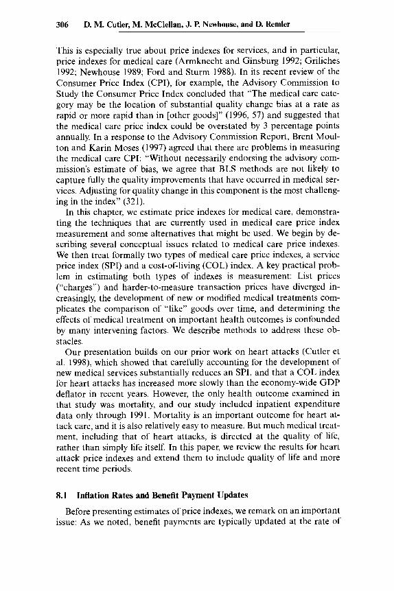
(2) U , ( t ) = C..d(t>.u,(H,[d,rn,(t)l,I: - p , ( t ) . m , ( t ) - T(t>)> d=l
where nd(t) is the probability that the person has disease d at time t; I/ is the consumer’s expected utility; H is the health of the person, which de- pends on the disease and the expected effects of medical care received; Y, is income (assumed to be constant over time); p,(t) is the vector of effective prices to person i of medical care at time t ; and T,(t) is lump-sum payments (insurance premiums or taxes) for medical services. The expression p . rn + T denotes spending on medical care, so that the second argument of the utility function is just the consumption of nonhealth goods.
We assume that medical services do not have independent consumption value, beyond their effect on health, and therefore do not include them directly in the utility function. While this assumption neglects the con- sumption value of medical care for nonhealth reasons, such as hotel-like features of hospitals and the “caring” role of the medical care process (Newhouse 1977; Fuchs 1993), it captures the predominant value of medi- cal care.
For simplicity, our specification does not capture some interactions be- tween current medical services and future utility. For example, elderly people whose life is prolonged but who are left partially disabled may suffer increased risk of future uninsured nursing home expense. The utility cost of this risk should be counted as a cost of current medical care con- sumption, just as the longer life is a benefit. However, we do discount fu- ture health benefits and costs to current dollars.
We wish to focus on the effects of changing technology and prices over time and not on the effects of individuals’ aging. Therefore, we abstract from the medical and economic effects of aging and implicitly analyze consumers with a constant age and income over time. Thus, we compare 65-year-olds in 1980 with 65-year-olds in 1990.
Consumer welfare may also change over time due to changes in disease incidence (Barzel 1968). Entirely new diseases such as AIDS may be added to the set of possible illnesses, and other diseases such as smallpox may be eliminated. Changes in lifestyles may change the incidence of a given set of diseases. For example, better diet, reduced smoking, and increased exer- cise have lowered the incidence of heart disease over time. We also abstract from these effects by estimating price indexes for a single disease. It is conceptually straightforward to apply similar methods to other diseases, and to reconstruct an aggregate price index from the specific illnesses. With a single disease, welfare is given by
(2‘) U ( t > = U W b ( t > l , Y - p ( t > . m ( t ) - T ( t ) )
With these assumptions, welfare changes are only a function of changes in medical treatments, their expected health effects, and payment over

312 D. M. Cutler, M. McClellan, J. P. Newhouse, and D. Remler
time. The question we pose is, How do these practice and payment changes affect the price of the medical services industry's product?
Following the literature on true cost of living indexes (Fisher and Shell 1972), we define the cost-of living index as the amount consumers would be willing to pay (or would have to be compensated) to have today's medi- cal care and today's prices, when the alternative is base period medical care and base period prices. The change in the COL index between to and t , , denoted C, is the amount of compensation required to equalize utility in those two states. It is implicitly defined from3
Taking a Taylor series expansion around sumption, and rearranging terms, we obtain
using x to represent con-
(4)
The first term on the right-hand side of equation (4) is the health benefit of changes in medical care, expressed in dollars, exactly the same concept as the benefit in a cost-benefit analysis. The second term is the change in the cost of medical care, the same concept as the cost in a cost-benefit analysis. If C is positive, the consumer is better off in period t , than he was in period to and conversely.
The Laspeyres COL index between period to and period t , is just the index of changes in C scaled by initial income5
3 . Fisher and Shell (1972) define the cost-of-living index in terms of expenditure functions. The income required to reach utility Uover time is COL = e(U,p,)/e(U,p,). This formulation is based on optimizing behavior. As discussed, medical care may not be chosen at the optimal level; excessive resources may be devoted to medical care due-to insurance and market fail- ures. When the level of medical care is chosen optimally, COL = 1 - [e( U, p,) - e( ?, p J e( U, p,) = 1 - C/Y,, and the two forms are equivalent. When the level of medical care IS not chosen optimally, equation (3) still represents a valid definition for the COL index, although its interpretation is somewhat different. In this case, the COL index still represents the change in income needed to keep people equally well off but under the constraint that medical care is allocated in the manner that it is actually allocated. Intuitively, we cannot use the machin- ery of optimization, such as expenditure functions. However, we can measure the extent to which people are better or worse off. 4. This is a first-order expansion which neglects the higher-order terms. For major techno-
logical innovations involving major changes in health outcomes and medical care expendi- tures, higher-order terms could be important. Qualitatively, such higher-order terms depend on various curvatures of the utility function and the health production function. Nonethe- less, the first-order terms capture the direct important welfare effects of medical care: the improvement in health and the loss of other goods.
5. The cost-of-living index can be formed using chain weights or other intertemporal aggre- gation methods.
Pricing Heart Attack Treatments 313
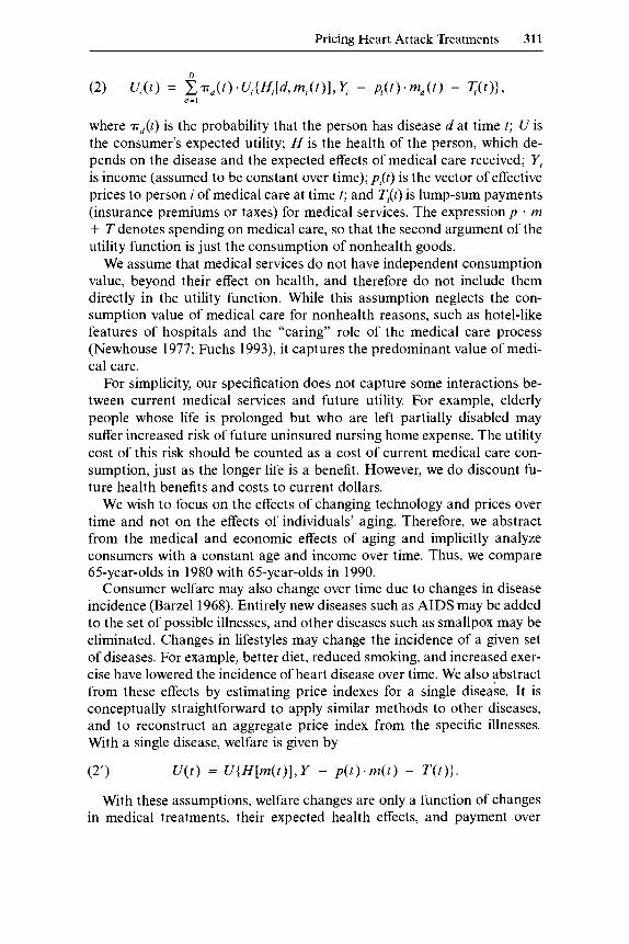
C coL ,o , r , = 1 - -.
r, It is important to note that the cost portion of the COL index is the change in the total cost of care, not the change in an SPI (i.e., p - m + T, not p ) . If consumers care only about health output, it is the total cost of treatment and its expected consequences for health that matter.
Because the COL index is a utility-based concept, the key question in implementing a COL index is what to assume about the relation between value and cost. In most markets, a reasonable assumption is that the mar- ginal consumer’s marginal valuation of the good equals its cost. Thus, we can link costs and value by observing how much consumers are willing to pay for the particular components in a bundled product. Indeed, this is the foundation of hedonic analysis (Griliches 197 1). In medical care markets, however, this is not a tenable assumption. When medical care decisions are made by patients who are insured at the margin or by health care providers whose interests may not coincide with those of the patient, there is no presumption that the marginal value of care equals its social cost. Thus, we cannot a priori use hedonic analysis to measure changes in the COL index.
A second approach is to specify a model for how consumption decisions are made. Then, using the observed path of consumption and spending, one could infer the change in the COL index. Fisher and Griliches (1995) and Griliches and Cockburn (1994) take this approach for generic drugs. However, many complex medical treatment decisions may be involved even in the treatment of a single health problem, and there is no generally accepted model for how such decisions are made. Therefore, we do not pursue this approach.
A third approach is to use direct evidence on the expected value of medical care in improving health. Then the COL index can be calculated using the measured cost and value differences directly. This is the approach we pursue here.
8.3 Heart Attacks: Brief Medical Background
A heart attack (acute myocardial infarction or AMI) is a sudden death of the heart muscle, which impairs the heart’s function in pumping blood through the body. The attack may be caused by lack of blood supply to the heart because of a blockage (occlusion) of the coronary arteries sup- plying blood to the heart. The location of the occlusion, as well as of other narrowings in the coronary arteries that create an elevated risk of further heart damage, can be determined by a diagnostic imaging procedure, car- diac catheterization. This procedure shows the degree of impairment of flow in the various coronary arteries supplying blood to the heart.

314 D. M. Cutler, M. McClellan, J. P. Newhouse, and D. Remler
Bypass
Cardiac Angioplasty Catheterization
Nothing Further
Medical Management
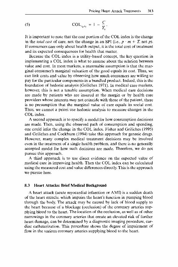
Fig. 8.1 Treatment of patients with a heart attack
If the catheterization shows that the blood supply is sufficiently im- paired, and if the expected clinical benefits are high enough, one of two revascularization procedures may be performed to improve the blood supply to the heart and prevent further damage (i.e., subsequent AMIs): coronary artery bypass graft (CABG) or percutaneous transluminal coro- nary angioplasty (PTCA). A CABG splices a piece of vein or artery taken from some other part of the body around the portion of the artery that is blocked. An angioplasty threads a balloon-like material into the artery and expands it, thereby opening the artery for the flow of blood.
If revascularization is not performed, the patient will be managed with drugs, counseling, and further monitoring, which we term medical man- agement. These options are diagrammed in figure 8.1. Although there are many other critical decisions in the treatment of AMI, we focus on the four treatment paths shown in figure 8.1: medical management and no catheterization, catheterization and no revascularization, a bypass opera- tion, and angioplasty.
8.4 The Data
Data to analyze medical care prices are particularly difficult to acquire, because one cannot just ask patients what procedures they had and how much they cost. The prevalence of insurance means that patients often do not know this information. Thus, medical care price data must come from providers, insurers, or both, each of which has particular complications. Added to this is the reticence of many providers (and insurers) to indicate how much they are receiving (or paying) for particular types of care. Fur- ther, the cost-of-living index requires data on medical outcomes, which are also difficult to obtain.
We use two sources of data in our empirical work. The first is a complete set of billable services, list prices (charges), demographic information, and

Pricing Heart Attack Treatments 315
discharge abstracts for all heart attack patients admitted to a major teach- ing hospital (MTH) between 1983 and 1994. The hospital that provided the data asked not to be named explicitly. The second data source is na- tional data on everyone in the Medicare population with a heart attack between 1984 and 1994.6 Because Medicare covers essentially all of the elderly, and since two-thirds of heart attacks occur in the elderly, Medicare data can provide a relatively comprehensive picture of the cost and out- comes of heart attacks in the elderly population.
Each of the data sets has advantages and disadvantages. The advantage of the MTH data is that we have the complete records from the hospital admissions; we know all the particular items that were given to the patient (often numbering in the hundreds). Because Medicare does not pay on a fee-for-service basis, the details of many services provided are not recorded by Medicare. All that is known reliably is the major treatments provided (catheterization, bypass surgery, and angioplasty). The advantages of the Medicare data are that the samples are larger, and they contain reimburse- ment information. For confidentiality reasons, MTH would not give us data on transactions prices for each patient-only list prices. In addition, the Medicare data can be linked to Social Security death records, which we have done, allowing us to record this important outcome for the Medi- care population. We do not have information on out-of-hospital outcomes for patients at MTH.
We created the sample of all patients with a new heart attack by identi- fying all claims with a primary diagnosis of heart attack (ICD-9 code 410), other than rule-out Heart attacks are a severe diagnosis, and essen- tially everyone with a heart attack who survives the immediate attack and thus receives any treatment will be admitted to a hospital; it is thus natural to start with the initial hospitalization. We also exclude readmissions for a previous heart attack in each data set. In the MTH data, we restrict the sample to those patients for whom the observed heart attack was their first treated at this hospital. In the Medicare sample, we choose patients who had not been hospitalized with a heart attack in the year preceding the admission of interest,
Treatments for a heart attack may extend over several weeks or months. For example, physicians may delay a cardiac catheterization or revascu- larization procedure to see if the patient’s heart muscle improves without these interventions. Indeed, there have been changes in the timing of these
6. In our earlier paper, we were only able to extend the data through 1991. This paper thus offers substantially more evidence on the price of heart attack care.
7. Some patients are admitted to a hospital to rule out a heart attack. Generally, these patients do not have a diagnosis of acute myocardial infarction (instead, unstable angina is the typical diagnosis). However, we also excluded patients admitted with a diagnosis of AM1 for less than three days, counting transfers, who were discharged alive, as such short lengths of stay would be extraordinary for a true elderly AM1 patient.

316 D. M. Cutler, M. McClellan, J. P. Newhouse, and D. Remler
procedures over time in the United States, with more of them being per- formed sooner after the heart attack occurs. To adjust for this, we define the “heart attack treatment episode” as all medical care provided in the ninety days beginning with the initial heart attack admission. We choose a ninety-day window because past analyses have suggested that this time period is adequate to capture essentially all of the initial treatments with- out including a large share of treatments for heart attack complications (McClellan, McNeil, and Newhouse 1994).
The Medicare data are available for the fee-for-service program only. Managed care organizations participating in Medicare have generally not submitted reliable utilization information to the government, and thus we exclude these people. For most of our time period, managed care enroll- ment was a small part of Medicare (less than 10 percent), so this omission is unlikely to have important effects on our results. In future years, how- ever, this problem could become increasingly important if steps are not taken to improve data reporting by managed care plans.8
Table 8.1 shows the sample sizes for the two data sets. The MTH data have about 300 heart attacks ann~al ly .~ The Medicare data have about 225,000 heart attacks annually. This number is relatively stable, even with the nearly 2 percent growth in Medicare enrollees annually, implying that heart attack incidence rates are falling.
The next columns of the table show the age and sex mix of people with a heart attack. The heart attack population is increasingly older over time. In 1984, 49 percent of heart attacks were in people aged 65-74; by 1994, this was down to 45 percent. The increased age of heart attack sufferers re- flects both the increased age of Medicare enrollees in general and the fact that younger people are taking better care of themselves over time (better diet and exercise) so that heart attack rates are falling in the younger el- derly. Slightly over half the heart attack population is male.
Medicare records indicate the amount of money Medicare paid the hos- pital for the care. We add up reimbursement in the year after the heart at- tack to form transactions prices. We use a one-year period to capture any related heart attack spending not picked up in the ninety-day period.
Measuring prices in the MTH data is more difficult. To facilitate expo- sition, a discussion of hospital accounting may be helpful. All hospitals have list prices or “charges” for very disaggregated services, such as minutes of operating room time or specific drugs. Until recently, the official price indexes for medical care, including hospital care, were based entirely on
8. The Balanced Budget Act requires Medicare managed care plans to submit complete encounter data in future years. However, it is not yet clear how soon this requirement will be implemented effectively.
9. We do not know if the patient had an earlier heart attack elsewhere. However, we do know if they were transferred to MTH from another hospital. We have experimented with restricting the sample to nontransfers, without important effect on the results.

Pricing Heart Attack Treatments 317
Table 8.1 Characteristics of the Medicare Population with Heart Attacks
MTH Data Medicare Data (1984-94) (1983-94)
Age Distribution (“YO) Number of Number of Percent
Year Heart Attacks Heart Attacks 65-74 75-84 85+ Male
1983 I984 1985 1986 1987 1988 1989 1990 1991 1992 1993 1994
156 209 205 222 242 214 206 309 365 47 1 566 477
-
233,284 233,886 223,573 227,894 223,178 218,052 220,643 235,827 240,573 175,985 238,480
-
49 48 48 47 46 46 46 46 46 46 45
-
39 39 39 39 39 40 40 39 39 39 39
-
12 13 14 14 14 15 15 15 15 15 16
-
51 51 51 50 50 50 50 51 51 52 51
Source: Data are from MTH and the Medicare program.
these charges. At MTH, these are the data we were provided, and we use them to mimic the historical Bureau of Labor Statistics (BLS) methods.’O But increasingly many payers do not pay list price. For example, Medicare and Medicaid pay hospitals an administered price; many Blue Cross plans receive discounts off charges, and managed care organizations often nego- tiate prices for broader groups of care, such as an all-inclusive per diem amount or an amount per admission. To approximate actual transactions prices, we use more accounting information. Profits for most hospitals- particularly not-for-profit major teaching hospitals, of which MTH is one-are close to zero (Prospective Payment Assessment Commission 1996). Thus, average accounting costs will roughly equal average reim- bursement. We therefore form a measure of average treatment “costs” for heart attack patients, which we use as a proxy for average transactions prices. Average treatment costs are formed by multiplying charges by the hospital- and department-specific “cost-to-charge’’ ratios. These ratios, provided to Medicare by the hospital, are used for certain Medicare billing purposes and are believed to be accurate.”
10. Transaction prices are not available for private payers for privacy reasons. Partly for this reason the BLS historically used list prices in the actual CPI.
1 1 . For ancillary departments such as laboratory or pharmacy the method multiplies charges that arise from that department (such as blood chemistry) by an overall department cost-to-charge ratio. Costs of room and board services (mainly nurses’ salaries) are computed directly and converted to an average daily rate. Overhead costs are allocated in a prescribed fashion for each department. Our method of deflating charges is fairly common in the litera- ture (Newhouse, Cretin, and Witsberger 1989).
318 D. M. Cutler, M. McClellan, J. P. Newhouse, and D. Remler
Throughout the paper all medical care inflation figures are the excess over general inflation. To measure general inflation we chose the GDP deflator, rather than the personal consumption expenditure deflator, in or- der to reflect opportunity cost in the overall economy. Use of another gen- eral inflation measure would, however, not substantively affect our results. All dollar figures are in 1991 dollars.
8.5 Changes in the Treatment of AM1
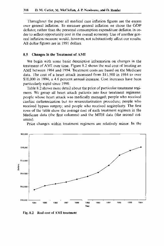
We begin with some basic descriptive information on changes in the treatment of AM1 over time. Figure 8.2 shows the real cost of treating an AM1 between 1984 and 1994. Treatment costs are based on the Medicare data. The cost of a heart attack increased from $11,500 in 1984 to over $18,000 in 1994, a 4.6 percent annual increase. Cost increases have been particularly rapid since 1990.
Table 8.2 shows more detail about the price of particular treatment regi- mens. We group all heart attack patients into four treatment regimens: people whose heart attack was medically managed; people who received cardiac catheterization but no revascularization procedure; people who received bypass surgery; and people who received angioplasty. The first rows of the table show the average cost of each treatment regimen in the Medicare data (the first columns) and the MTH data (the second col- umns).
Price changes within treatment regimens are relatively minor. In the
I 1984 1985 1986 1987 1988 1989 1990 1991 1992 1993 1994
Year
Fig. 8.2 Real cost of AM1 treatment

Table 8.2 Share of Patients and Expenditures for Treatment Regimens
Medicare Sample MTH Sample
Treatment Regimen 1984 ($) 1994 ($) Change” (%) 1983-85 ($) 1992-94 ($) Change” (%)
Medical management Catheterization only Angioplasty Bypass surgery
Medical management Catheterization only Angioplasty Bypass surgery
10,155 15,881 26,661 29.116
89 6 1 5
Average cost of treatment regimen 13,190 2.6 13,900 15,613 -0.1 15,290 19,309 -3.2 16,124 36,564 2.3 31,431
Share of patients receiving treatment regimen (%) 53 -3.6 65 16 1.0 20 11 1.6 3 15 1 .o 11
1 1,769 15,105 18,441 50.874
23 21 30 21
-1.8 -0.1
1.5 3.4
-4.1 0.1 3.0 1.8
Note: Costs are in 1991 dollars, adjusted using the GDP deflator. Thange is annual percentage points for treatment shares and annual percent for costs.

320 D. M. Cutler, M. McClellan, J. P. Newhouse, and D. Remler
Medicare data, prices for medical management and bypass surgery rose in real terms, but the annual increases are small. The price of catheteriza- tion and angioplasty fell substantially-by 0.2 to 3.6 percent, respectively. In each case, the reduction in reimbursement was by design. In 1984, angioplasty was new and was perceived to be expensive. It was thus placed in a relatively highly reimbursed category. As the procedure spread and Medicare officials learned that it was less expensive than previously thought, angioplasty was moved to a less expensive reimbursement cate- gory. Payments for cardiac catheterization only fell as more catheteriza- tions were done in the initial hospital visit or on the same admission as more expensive revascularization procedures. In the MTH data, costs of medical management and cardiac catheterization fell in real terms, while angioplasty and bypass surgery rose. Only the bypass surgery increase was large, however, and we suspect that some of this reflects changing patient demographics into and out of MTH over time. It is clear from both the Medicare and MTH data, however, that price increases do not explain the growth of heart attack spending.
The next rows show the change in the utilization of these procedures over time. AM1 treatment changed markedly during the period of our study. In both samples, the use of the two invasive procedures rose sub- stantially. In the mid-1980s only about 10 percent of elderly heart attack patients received at least one of the three major procedures (35 percent at MTH, including nonelderly). By the mid-l990s, nearly half of elderly heart attack patients received one (75 percent at MTH). MTH is more intensive than the average hospital (as expected), but the trends at MTH are similar to those for the nation as a whole.
As an accounting matter, the increase in treatment intensity is the pre- dominant factor in explaining the growth of medical spending. We make this formal with an accounting identity. The average cost of treating a heart attack is the sum over treatment regimens of the share of patients receiving each treatment times the average cost of that treatment, or
To a first approximation, then, the change in treatment costs” is given by
(7)
Table 8.3 shows the amount of the increase in treatment costs that can be explained by price changes and quantity changes. The table shows that a large share of the increase in spending is a result of changes in the type of treatments patients are receiving; a much smaller share is a result of
12. This is an approximation because it ignores the covariance term.

Pricing Hear t Attack Treatments 321
Table 8.3 Decomposition of the Growth of Heart Attack Spending
Measure Medicare MTH
Increase in average cost ($) 6,515 8,452 Increase resulting from price changes ($) 2,977 125
Increase resulting from quantity changes ($) 5,109 4,658 [46%] [2%]
[780/0] [55?'0]
Note: Based on table 8.2. Numbers in brackets are the share of the total increase that can be explained by that factor. Percents do not add to 100 percent because of covariance term.
increases in the cost of a given treatment regimen. In the Medicare data, for example, 78 percent of cost increases result from increasing intensity of treatments. The price component is relatively large as well (46 percent), but this is somewhat deceptive; angioplasty, which was essentially nonexis- tent in 1984, fell in price substantially over this period while bypass sur- gery, which was much more common, rose in price. If we use 1991 quantity weights instead of 1984 quantity weights, the component of cost increases resulting from price increases would be less than half as large.
The MTH data suggest that only 2 percent of spending increases result from cost increases. Increases in the intensity of treatment, in contrast, explain over half of the increased cost of heart attack care.
These results presage our later result that if conventional price indexes used the treatment regimen approach they would not find a substantial increase in medical spending over time. This finding also highlights the importance of quality adjustment. Doctors are providing these additional high-tech services at least in part because they believe them to be valu- able-they increase survival or reduce morbidity. To form an accurate price index, we need to value these changes in quality.
8.6 Service Price Indexes
8.6.1 Disaggregated Service Price Indexes
Prior to 1997, the official CPI for medical care was based on disaggre- gated service prices (Cardenas 1996).13 The goods priced and the hospitals in the sample were kept constant, if possible, for five years, at which time both hospitals and goods were resampled. Figure 8.3 shows the real med- ical care CPI from 1983 to 1994 (when this method was followed), and table 8.4 shows mean growth rates. Over this time period the real medical care CPI rose 3.4 percent annually. The real hospital component of the CPI increased even more rapidly, 6.2 percent annually.
13. The PPI for medical care used aggregated service prices beginning in 1993.

1.5
1.4
1.3
- r
A - b 1.2
:: c -
1.1
1 .o
0.9 1983 1984 1985 1986 1987 1988 1989 1990 1991 1992 1993 1994
Year
Fig. 8.3 Real consumer price indexes
Table 8.4 Summary of Price Indexes
+Synthetic CPI -Charges
Index Real Annual Change (“A)
Service price indexes Disaggregated service price indexes
Official medical care CPI 3.4 Hospital component 6.2
Room 6.0 Other inpatient services 5.7
Synthetic CPI for MTH-charges 3.3 Synthetic CPI for MTH-costs 2.4
Fixed basket index 2.8
Annual chain index 0.7
Fixed basket index 2.31- 1.3 Annual chain index 1.710.4
Heart attack episode-disaggregated price index
Five-year chain index 2.1
Aggregated service price indexes (Medicare/MTH)
Cost of living index Years of life -1.5
[-0.2, -13.71
[-0.3, -16.81 Quality of life -1.7
Nores: Service price indexes for the 1983-94 period, with the exception of other inpatient services, which begins in 1986. Aggregated SPIs for Medicare data and cost-of-living index are for 1984-94. The values in brackets for the cost-of-living index are based on higher and lower estimates of the net value of a life year. Real changes are estimated using the GDP de- flator.

Pricing Heart Attack Treatments 323
Although the CPI resamples goods every five years, it traditionally did not price the goods used by an average patient. For example, it always priced a one-day stay, independent of trends in actual length of stay. When actual care changed (for example, shorter stays), no adjustment was made to the index. An alternative methodology is to choose the average patient in each year and price the services used by that average patient over time. If we resample patients frequently enough, changes in the care provided would be incorporated in the index (Scitovsky 1967).
The difficulty with sampling patient bills over time is that the set of goods provided changes; some goods disappear and others newly appear. The detailed MTH data permit the extent of market basket change to be quantified. In consecutive years, we can match services for 98 percent of charges. But over five years, we match only 42 percent of charges, and over 11 years (the maximum span of our data), we match only 27 percent of charges. Many of the changes are straightforward (e.g., a different code for an additional intensive care unit); when we allow for this, our ability to match charges increases substantially. Over the eleven-year period 78 per- cent rather than 27 percent of expenditures can be matched.I4
Truly new goods pose a more difficult problem. For example, intra- aortic balloon pumps-small pumps inserted near the heart that can tem- porarily help the heart pump blood-did not exist in 1987 but had grown to almost 1 percent of heart attack spending by 1994. Like the BLS we link such new goods as we are able, but make no adjustment for potential quality change (U.S. Department of Labor 1992).15
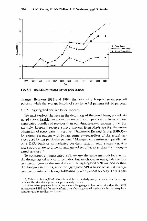
The upper line in figure 8.4 and the next row of table 8.4 show the disaggregated SPI calculated using the market basket for the average pa- tient in the initial year. This index increases 2.8 percent annually in real terms, close to the increase in the cost-based synthetic CPI, as we would expect. The next rows of the table examine the effects of resampling pa- tients more frequently. Using a Laspeyres index that resamples patients every five years the annual increase in real prices is only 2.1 percent, and a chain-weighted Laspeyres index (annual resampling) increases only 0.7 percent. The bias from fixed weights is thus substantial. The difference in these indexes results almost entirely from the weight placed on room
14. Over five years the figure is 85 percent; the one-year figure remains 98 percent. 15. The BLS treats new and obsolete goods using three possible methods. In some cases,
a new good is considered to be a direct and fully equivalent replacement for an old good (termed direct comparability). In other cases, quality adjustments are made for the shift from an old to a new good (termed direct quality adjustment), although this method is rarely used in practice due to the difficulties in quantifying quality improvements. Other new goods are linked into the old index, which is equivalent to assuming that the quality-adjusted price change in the substitution period is exactly equal to the price change of the other goods in the category. For our longer indexes, linking underweights the kinds of goods that appear and disappear frequently, such as pharmaceuticals, and overweights the kinds of goods that exist over long periods, such as intensive care unit rooms. The BLS is trying to integrate quality changes into the new PPI, as we discuss in the conclusion.
324 D. M. Cutler, M. McClellan, J. P. Newhouse, and D. Remler
1 3 -
- 1.2
4 = B
1.1 -
1.0
0.9 7
--
t 5 Year Chain Weight
charges. Between 1983 and 1994, the price of a hospital room rose 60 percent, while the average length of stay for AM1 patients fell 36 percent.
8.6.2 Aggregated Service Price Indexes
We next explore changes in the definition of the good being priced. As noted above, health care providers are frequently paid on the basis of more aggregated bundles of services than our disaggregated indexes price. For example, hospitals receive a fixed amount from Medicare for the entire admission of every patient in a given Diagnostic Related Group (DRG)- for example a patient with bypass surgery-regardless of the actual ser- vices used by the particular patient.I6 Managed care insurers typically pay on a DRG basis or an inclusive per diem rate. In such a situation, it is more appropriate to price an aggregated set of services than the disaggre- gated services.”
To construct an aggregated SPI, we use the same methodology as for the disaggregated service price index, but we choose as our goods the four treatment regimens discussed above. The aggregated SPIs are noisier than the disaggregated SPIs, since the aggregated SPI is based on actual average treatment costs, which vary substantially with patient severity. This is par-
16. This is a bit simplified. More is paid for particularly costly patients than for average patients. But this description is approximately correct.
17. Even when payment is based on a more disaggregated level of service than the DRG, an aggregated SPI may be more informative if the aggregated service is a better proxy for a constant-quality medical care good.

Pricing Heart Attack Treatments 325
1.5
1 4
1.3
- r
f - e 1.2 x
1.1
1 .o
0.9 ~~
1983 1984 1985 1986 1987 1988 1989 1990 1991 1992 1993 1994
Year
Fig. 8.5 Real aggregated service price indexes
ticularly true for the MTH data, where the sample sizes are smaller.'* We thus focus predominantly on the aggregated SPIs for Medicare.
Using both fixed basket and annual chain-weighted Laspeyres price in- dexes, aggregated SPIs grow less rapidly than most of the disaggregated SPIs (fig. 8.5 and table 8.4). The fixed basket index increased 2.3 percent per year in the Medicare data, and the annual chain-weighted index in- creased 1.7 percent per year. The changes at MTH are smaller. Our pre- ferred estimate of real price increases using an aggregated SPI is therefore about 1.5 percent annually. This is approximately 1.0 to 2.0 percentage points below a price index reflecting historical BLS methods.
The increase in the aggregated SPI for Medicare in the 1984-94 period is greater than the increase in the 1984-91 period reported in our earlier paper (Cutler et al. 1998). In that paper, we reported a growth of the aggre- gate SPI using Medicare data of 1.1 percent (the fixed weighted index) and 0.6 percent (the chain-weighted index). The higher inflation rates reported here reflect the much more rapid growth of Medicare spending after 1991 than prior to 1991. Figure 8.5 shows the growth of the aggregated price index over time. In 1992, the inflation rate with the Medicare data was nearly 8 percent, followed by 3 percent in 1993 and 2 percent in 1994. As
18. The MTH index is particularly variable because annual fluctuations in the average severity of admissions affect the average cost in each category and therefore this index. To eliminate some of these fluctuations, we formed an alternative price index using a three-year moving average of costs for each treatment regimen and the share of patients receiving each treatment regimen. The resulting chain-weighted index fell 0.1 percent annually.

326 D. M. Cutler, M. McClellan, J. P. Newhouse, and D. Rernler
with any series, cumulative inflation rates will be more variable over shorter time periods than over longer time periods.
8.7 Cost-of-Living Index
Forming a cost-of-living index is more complicated than forming an SPI because one must price improvements in health rather than just specific medical services. Thus, we have to measure and price health improvements after a heart attack. Since outcome data are most readily available for the Medicare sample, we use only the Medicare data to form the cost-of- living index.
As noted above, the demographics of the heart attack population are changing somewhat over time. To account for this, we adjust all of our estimates for changes in the age and sex mix of the population. We group the population into five age groups (65-69,70-74,75-79,80-84, and 8 5 - t ) and two sex groups, for a total of ten demographic cells. The data are adjusted to the average demographic mix of the heart attack population over the eleven-year period.I9 We would like to adjust for clinical charac- teristics of the heart attack as well (the extent of blood flow, other compli- cations and/or comorbidities), but such data are either not present on the discharge abstract (e.g., the extent of blood flow) or are not coded reliably (e.g., complications may be recorded less often for patients who die during the hospitalization). We thus adjust for demographics only. Other clinical reviews (e.g., McGovern et al. 1996) suggest that the severity of heart at- tack patients has not changed much since the mid-1980s.
8.7. I Length of Life
We begin with data on the length of life after a heart attack. Figure 8.6 shows survival rates over time (adjusted for demographics), based on the year of the heart attack. We show cumulative mortality rates on the day of the heart attack, by ninety days, one year, two years, three years, four years, and five years after the heart attack. We show survival for people with heart attacks in 1984, 1987, 1991, and 1994. Because the Social Secu- rity data are only available through 1995, we cannot compute some of the mortality rates; for example, five-year mortality rates for people with a heart attack in 1994 would require death records through 1999, which did not yet exist when we carried out this work. Still, we can assemble a time series of long-term changes in mortality for many years.
Mortality rates after a heart attack have declined substantially over time. In the first day after the heart attack, for example, mortality rates
19. In our earlier paper (Cutler et al. 1998), the data were adjusted to the demographic mix between 1984 and 1991. Thus, the data are not strictly comparable in the two analyses, although all of the trends are exactly the same.

Pricing Heart Attack Treatments 327
0.7
0.6
0.5 - c
t!
8
1 0.3
0.4 - 2
e B
0.0 1 1 Day 90 Days 1 Year 2 Years 3 Yean 4 Yean 5 Yean
Time Atter Heart Attack
Fig. 8.6 Cumulative mortality rates after a heart attack
4-1987 -A- 1991
were 9.0 percent in 1984, 8.2 percent in 1987, 6.6 percent in 1991, and 5.7 percent in 1994. Mortality rates at one year after the heart attack have fallen by 9 percentage points. As figure 8.6 shows, the decline was particu- larly pronounced in the mid-l980s, but mortality rates fell in all years.
Determinants of Mortality Improvement
The central question about the improvement in the length of life is whether it results from improved medical care or other factors. Heiden- reich and McClellan (chap. 9 in this volume) look at this issue in some detail. They find considerable evidence that medical innovations are an important contributor to improved survival, and in particular that they explain the bulk of survival during the acute treatment period. We summa- rize their results briefly.
Heidenreich and McClellan first document the reduction in AM1 mor- tality over time. Between 1975 and 1995, acute heart attack mortality (in the first thirty days after the AMI) fell from 27.0 percent to 17.4 percent, a decline of nearly 2 percent per year. To analyze why heart attack mortal- ity fell so rapidly, Heidenreich and McClellan review the (literally) hun- dreds of published studies and meta-analyses of heart attack treatments and their effectiveness.
Table 8.5 summarizes the evidence on the effect of acute treatments on AM1 mortality. The first column reports the mortality odds ratio of the technologies, using results from clinical trials and meta-analyses. Many of the technologies have quite substantial health impacts (values below 1) although some of the technologies are now believed to be harmful, such

328 D. M. Cutler, M. McClellan, J. P. Newhouse, and D. Remler
Table 8.5 Estimated Acute Mortality Benefits of Changes in Acute Treatment of AM1
Therapy Change in Use, Share of Total
Odds Ratio 1995-75 (YO) Improvementd (0%)
Pharmaceuticals Beta blockersb Aspirinb Nitrates Heparin/anticoagulants Calcium-channel blockers Lidocaine Magnesium ACE inhibitorsb Thrombolyticsb
Procedures Primary PTCAb CABG
TotalLMajor treatments only All treatments
0.88 0.77 0.94 0.78 1.12 1.38 1.02 0.94 0.75
0.50 0.94
29.0 60.0 30.0 4.0
31.0 -15.0
8.5 24.0 31.0
9.1 6.7
6.1 27.5
-5 .5 -0.5 -7.3 10.7
-0.3 2.7
16.1
9.8 0.6
62 60
Note: Based on data analysis in Heidenreich and McClellan (chap. 9 in this volume). “Percentage of 1995-75 decrease in AM1 case fatality rates explained by changes in use of each treatment. bMajor treatment.
as calcium-channel blockers and lidocaine. Heidenreich and McClellan define as “major technologies” those treatments where the clinical trial evidence is particularly advanced-beta blockers, aspirin, ACE inhibitors, thrombolytics, and primary PTCA.
The second column shows the change in the share of patients receiving these treatments over time. Treatment changes have been substantial. Thrombolytics, for example, were not used in heart attack care in 1980, but were used in almost one-third of heart attacks by 1995. The use of aspirin, beta blockers, and heparin also increased. Calcium-channel blocker use increased rapidly in the early 1980s and then fell, following the publication of studies documenting potentially harmful effects of their use in acute management. Use of lidocaine and other antiarrhythmic agents also fell over the time period, in conjunction with new information on their potential harmfulness for typical AM1 patients. And as noted above, both PTCA and bypass surgery increased in use by a substantial amount.
The third column shows the share of the total mortality change between 1975 and 1995 attributable to these treatments. Two summary estimates are presented in the last rows of the table. The first estimate uses evidence on the major treatments only. By this estimate, 62 percent of the reduction in AM1 mortality in the past twenty years is attributed to changes in acute

Pricing Heart Attack Treatments 329
treatments. The second estimate uses all of the technologies; the attribut- able share is very similar, 60 percent.
Three drug therapies in particular account for the largest improvements in heart attack mortality-aspirin, thrombolytics, and beta blockers. In- deed, beta blocker use alone accounts for over one-quarter of the mortality decline and use of thrombolytics accounts for an additional 15 percent. The development and spread of PTCA explains nearly 10 percent of the mortality decline.*O
Heidenreich and McClellan also review the more limited evidence on other sources of improvement in acute mortality over time. Though changes in monitoring methods were important sources of mortality im- provements in the 1960s and early 1970s (Goldman and Cook 1984), they have been less important recently. Coronary care units, for example, had largely diffused by the mid- 1970s, and right-heart (pulmonary artery) cath- eterization for functional assessment, which has spread rapidly, does not result in clear survival improvements.
Changes in prehospital care may be more important. Emergency 91 1 systems and (recently) enhanced 91 1 systems have become more widely available, and the content of ACLS procedures has evolved. Several stud- ies have failed to document improvements in mortality following activation or enhancement of 91 1 systems, however. Similarly, time between hospital arrival and the delivery of key AM1 treatments (thrombolytics, primary angioplasty) appears to have declined, although again the evidence on how important this is in increasing survival is limited. It is likely that improve- ments in prehospital care and reductions in time to treatment have led to a modest improvement in AM1 mortality, perhaps 5-10 percent, but this conclusion is speculative.
Changes in the type of AMIs admitted to hospitals might also explain about 10 to 20 percent of improved survival over this period, particularly between 1975 and 1985. The average age of AM1 patients in the Minnesota and Worcester registries, and the proportions of male and female patients were essentially constant. Data on specific measures of heart attack sever- ity (such as anterior MIS, non-Q-wave infarcts, and high blood pressure at admission) suggest a modest improvement in severity of heart attacks.
Altogether, changes in acute treatment, prehospital care, and patient characteristics may explain as much as 80 percent of the total improve- ment in acute mortality for heart attacks. The remaining 20 percent likely
20. The finding that pharmaceutical use explains a larger share of mortality declines than intensive surgical procedures may understate the role of these technologies in contributing to mortality reductions, since it does not account for learning by doing, which will be more important in surgical procedures than in pharmaceuticals. On the other hand, much of the improvement in learning by doing involves reducing the risk of complications from the proce- dure-so that patients expected to have relatively modest benefits become better candidates as experience improves.

330 D. M. Cutler, M. McClellan, J. P. Newhouse, and D. Remler
results from other technologies that we have not studied in detail, improve- ments in physician acumen in applying technologies, differential diffusion in subgroups of heart attack patients (with differential effects), and miscel- laneous other factors.
Long-term survival rates are also influenced by postacute care. As figure 8.6 shows, postacute mortality for heart attack patients is substantial. Many innovations have occurred in postacute treatment of heart attack patients, including expanded cardiac rehabilitation programs as well as drug therapies such as ACE inhibitors and anticoagulation therapy. How- ever, few studies exist that quantify the effects of long-term therapies for heart failure patients. The best evidence exists for ACE inhibitors, but lim- ited quantitative data on the changes in heart failure prevalence after heart attacks makes it difficult to quantify these important effects. The same is true about secondary prevention of AM1 through diagnostic procedures for risk stratification, risk factor counseling, pharmacologic therapies, and invasive procedures. Once again, studies show that many of these tech- niques result in significant reductions in long-term mortality after heart at- tacks, but data on changes in utilization or efficacy of these therapies are lacking.
Taken together, the factors discussed here suggest that innovations in each of primary prevention, acute and postacute management, and sec- ondary prevention have led to substantial reductions in acute and long- term AM1 mortality. We cannot quantify each of the components of im- proved long-term health, but medical interventions appear to be particu- larly important.
In light of this evidence, we assume that the mortality improvements shown in figure 8.6 are the outcome of medical treatments. This assump- tion is essentially correct for mortality improvements since 1985, and is largely correct over the entire 1975-95 period. As we show in other work (Cutler et al. 1998), assuming that only a relatively small share of the mor- tality improvement results from medical interventions does not apprecia- bly affect our results about cost of living indexes.
Cost-qf Living Price Indexes
To estimate the price index for heart attack care, we need to turn these mortality improvements into changes in the value of remaining life. We start with some notation. Denote the share of people who die in period s after a heart attack occurring in year t as d,(t). The values of s correspond to our intervals above: one day after a heart attack, ninety days after a heart attack, and so on. We assume that people who died in each interval died exactly halfway through that interval. Thus, people who died between one day and ninety days after a heart attack lived exactly 1.5 months, people who died between ninety days and 365 days after a heart attack died after 7.5 months, and so on. Denote the length of life for people who

Pricing Heart Attack Treatments 331
died in each interval as I, and the value of a year of life as IZ For the moment, we assume that V is constant over time and across people; we discuss this assumption in more detail below.
The present value of remaining life is given by
where r is the real discount rate. In our analysis, we assume a real discount rate of 3 percent; the results are not particularly sensitive to this assump- tion.
To estimate equation (8) empirically, we need to determine the share of people dying in each interval after a heart attack. Our data give us much of this information. If the cumulative mortality rate after a heart attack is CM,(t), the share of people dying in interval s is just CMs(t) - CM,-,(t). But we do not know the cumulative mortality rate for every interval s in every year-for example, five years after a heart attack that occurred in 1994. To estimate these cumulative mortality rates, we begin by forming the annual mortality hazard. For example, the hazard rate between years 2 and 3 is the share of people alive at the end of year 2 who die in year 3. We form the mortality hazard rate for as long a time as we are able. For example, in 1994, we are able to form the mortality hazard rate between ninety days and one year for every calendar year, the mortality hazard rate between one year and two years for each calendar year through 1993, the mortality hazard rate between two years and three years for each calendar year through 1992, and so on.
Consistent with the reduction in cumulative mortality rates, the mortal- ity hazard rates are declining over time. For example, the hazard rate be- tween one year and two years after an AM1 was 13.1 percent in 1984 and 10.7 percent in 1993. We need to forecast this hazard rate through 1994. To be conservative, we assume that the mortality hazard rate in 1993 (10.7 percent) continued through 1994. Since the mortality hazard rate was fall- ing up through 1993, and mortality hazard rates at durations shorter than two years were falling between 1993 and 1994 as well, this assumption almost surely understates the reductions in mortality hazard rates in 1994. By understating the reduction in the mortality hazard rate, we understate life expectancy in later years of the sample and thus overstate the change in the cost-of-living index. We use the constant mortality hazard rate as- sumption to forecast all of the unknown mortality hazard rates through five years after a heart attack.
We then need to determine life expectancy for a person surviving five years after a heart attack. Our data provide no evidence on this. We again make a conservative assumption. We start with national data on survival in 1984, matched by age and sex to the demographic mix of the heart

332 D. M. Cutler, M. McClellan, J. P. Newhouse, and D. Remler
attack population. For this population, we first find the mortality hazard rate between four and five years after the age at which they match the heart attack population. This mortality rate is 8.6 percent. We then compare this to the mortality hazard rate between four and five years after the heart attack for people with a heart attack in 1984. This mortality rate is 10.4 percent, or 21.5 percent above the mortality hazard rate for the population as a whole. We assume that for every subsequent year after a heart attack, people who have had a heart attack have a 21.5 percent greater mortality hazard rate than people who have not had a heart attack. We can then simulate future survival rates for people who have survived five years after a heart attack. These calculations suggest that people who have lived five years after a heart attack can expect to live another seven years on average.
We assume that this seven-year additional survival is the same for a person with a heart attack in every year. This is a conservative assumption, since mortality hazard rates up to five years are declining over time, and there is no reason to think that mortality reductions would cease after five years. By making this assumption, we likely understate gains in survival over time and thus likely overstate the cost-of-living index.
The first column of table 8.6 shows life expectancy after a heart attack. Life expectancy rose from five years in 1984 to six years in 1994. The increase in life expectancy was particularly concentrated in the 1987-1 990 period. In those three years, life expectancy rose by six months, compared to two months before and four months after.
To determine the value of this life extension, we need to know the worth of a year of life. This is a venerable question in the health economics litera- ture (Viscusi 1993; Tolley, Kenkel, and Fabian 1994). There are three ap- proaches that have been used to estimate the value of life. The first ap-
Table 8.6 Cost-of-Living Index for Heart Attacks, 1984-94
Value of Additional Life for Dollar Value of a Life Year of:
Medicare Spending ($1
Year Life Expectancy $10,000 $25,000 $100,000 Cost Change
I984 1985 1986 1987 1988 1989 1990 1991 1992 1993 1994
5 yrs 0 mnths 5 yrs 0 mnths 5 yrs 1 mnth 5 yrs 2 mnths 5 yrs 4 mnths 5 yrs 6 mnths 5 yrs 8 mnths 5 yrs 9 mnths 5 yrs 10 mnths 6 yrs 0 mnths 6 yrs 0 mnths
-
625 978
1,939 3,200 4,751 5,690 6,847 7,650 8,648 8,639
~~
1,564 2,445 4,847 8,001
11,877 14,226 17,116 19,124 2 1,620 21,597
6,254 9,780
19,390 32,003 47,510 56,903 68,465 76,495 86,482 86,388
1 1,483 12,066 12,395 12,673 13,123 13,588 14,186 15,293 16,867 17,581 18,165
583 912
1,190 1,640 2,105 2,703 3.810 5,385 6,098 6,682
Source: Data are from the Medicare population

Pricing Heart Attack Treatments 333
proach is contingent valuation-asking people the value they are willing to pay for increased length of life. This approach suffers from the usual drawbacks of surveys, however, including the fact that people have fre- quently not thought about the question in advance. The second approach is the compensating differentials approach. In many situations, people have to make job choices where risk of injury or death varies across jobs. On average, people get paid more to work in riskier jobs than in safer jobs. The risk premium that people need to be compensated to work in riskier jobs is an estimate of the value of life. The third approach is to use data on individual purchases of safety devices (for example, airbags in cars). By knowing the probability that an airbag will save one’s life, researchers can back out the implicit value people place on their life.
A rough consensus from this literature (Tolley, Kenkel, and Fabian 1994) is that life for a prime-age person is worth about $3 million to $7 million, or about $75,000 to $150,000 per year. Cutler and Richardson (1997, 1998) suggest a value for the population as a whole of $100,000 per year of life.
It is not immediately apparent whether we should use this estimate in our research. We are evaluating life years for the elderly, while most stud- ies look at life years for prime-age people as well as the elderly. One might value a life year more when one has young children, for example, than when one does not. Indeed, surveys conducted by Murray and Lopez (1996) show that people value years of life for middle-aged people the most, relative to years of life for the young or the old. Similarly, the life years that we are evaluating are after a heart attack, and their quality might be lower than years of life without a heart attack (a topic we return to below). For these reasons, we make a benchmark assumption that a year of additional life is worth $25,000. To evaluate the sensitivity of these results, we alternately assume a year of life is worth $10,000 and $100,000.
The next three columns of table 8.6 show the implied change in the value of life. Under our benchmark assumption, the additional years of life added between 1984 and 1994 are worth over $20,000. This varies between $9,000 when we assume a life year is worth $10,000 and $86,000 when we assume a life year is worth $100,000.
Cost-BeneJit Analysis und the Cost-oflLiving Index
To form the cost-of-living index, we need to compare this additional value of life with the cost of producing those additional years. To deter- mine these costs, we use the data on Medicare spending in the year after a heart attack. The next column of table 8.6 shows average Medicare costs of treating a heart attack, in 1991 dollars.*’ Medicare spending on heart
21. Costs should be put in the same dollars as the value of a life. It is not clear what year’s dollars the $25,000 assumption applies to. Since 1991 is about the middle of our data (and is the year we used in our previous research), we assume the $25,000 is the value of a life in 199 1 dollars.

334 D. M. Cutler, M. McClellan, J. P. Newhouse, and D. Remler
attacks is substantial-nearly $20,000 by 1994. And as noted above, spending has increased over time, by $6,682 between 1984 and 1994. The increase in Medicare spending is shown in the last column of the table.
Comparing the increase in the value of life with the increase in Medicare spending yields a clear conclusion: The value of increased longevity is greater than the increase in spending required to produce that additional life. Using our benchmark estimates, the net value of additional life be- tween 1984 and 1994 is $14,915 ($21,597 - $6,682). Under the low and high assumptions for the value of a life year, the net gains are $1,957 and $79,706, respectively.
The fact that the estimated value of improvements in heart attack mor- tality is greater than the total increased expenditures has a direct implica- tion for price index measurement: it implies that the cost of living for heart attacks is falling. To turn these estimates into a price index, we need to scale them by the cost of reaching the baseline level of utility in 1984. On net, the elderly consume roughly $25,000 per person per year (including medical care expenses). Thus, we assume that baseline resources involved in providing for the elderly is $25,000 per year, times the five years of expected survival for an elderly person with a heart attack, or $107,000 in present value.
Figure 8.7 shows the implied cost-of-living index. Under our benchmark assumption, the cost-of-living index falls by 1.5 percent per year. Using the conservative estimate of the value of a year of life, the decline is 0.2 percent, and using the higher value yields a decline of 13.7 percent. Thus.
1 0 ~
0 8 ~
- r f
0.6 -
0.4 -
0.2
00 1984 1985 1986 1987 1988 1989 1990 1991 1992 1993 1994
Year
Fig. 8.7 Cost-of-living index

Pricing Heart Attack Treatments 335
in each case the cost-of-living index is falling. This is in marked contrast to conventional medical care price indexes, which have been rising rapidly in real terms over this period.
8.7.2 Quality of Life
In addition to the length of life, people also care about its quality. Qual- ity of life was mentioned implicitly in the previous section; in this section, we discuss it explicitly. There are several dimensions to quality of life. Phys- ical health is one of them-can the individual ambulate independently? Can they manage tasks of daily living? Do they need specialized nursing care? Mental health is also important: Depression is a commonly reported complication after heart attack, and a few recent studies have even found an association between antidepressant treatment and heart attack sur- vival.
To make sense of these differing components to quality of life, we think of quality of life on a 0 to 1 scale, where 0 is death and 1 is living in perfect health. If we can estimate quality of life after a heart attack, we can then form the expected number of quality-adjusted life years for a person, rather than just the expected number of years remaining.22
To do this, we need to be more precise in our definitions. We denote the quality of life in any year as Q, which ranges from 0 to 1. For data reasons (discussed below), we assume Q is the same in each year after a heart at- tack. We define V as the value of a year in perfect health. Then, the present value of remaining quality-adjusted life years is
(9) VQdJ
I (1 + r).T PV[quality-adjusted life years] = C
To measure quality of life for heart attack patients, and quantify how it has changed over time, we examine a number of different measures. One aspect of quality of life is the need for additional medical care. Heart at- tack patients who fare poorly may need to be readmitted to the hospital for one of several reasons. The person may have a subsequent AM1 or develop serious ischemic heart disease (IHD) symptoms (including severe chest pains, palpitations, and other symptoms that resemble those of a heart attack) or they may develop congestive heart failure (insufficient pumping function by the heart, causing a reduced exercise tolerance and even severe difficulty breathing if fluid “backs up” into the lungs).
Table 8.7 and figures 8.8 to 8.11 show trends in readmission for these
22. Other approaches also exist for assessing the value of survival years in less than perfect health. For example, Murray and Lopez (1996) favor the use of disability-adjusted life years (DALYs), and other cost-effectiveness experts have favored healthy-year equivalents (HYEs). For purposes of the expected utility calculations underlying the COL index, however, quality- adjusted life years are the most natural index.
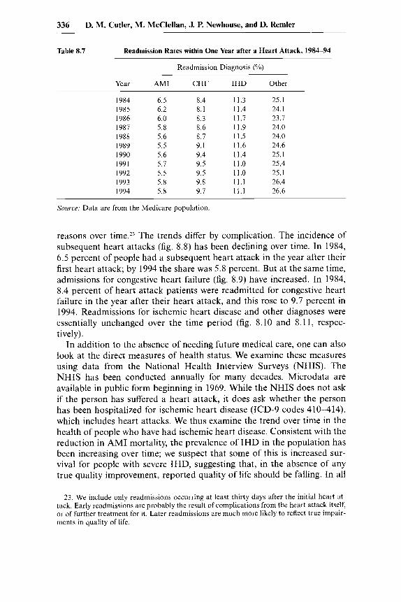
336 D. M. Cutler, M. McClellan, J. P. Newhouse, and D. Remler
Table 8.7 Readmission Rates within One Year after a Heart Attack, 1984-94
Readmission Diagnosis (YO)
Year IHD Other
1984 1985 I986 1987 1988 1989 1990 1991 1992 1993 1994
6.5 8.4 6.2 8.1 6.0 8.3 5.8 8.6 5.6 8.7 5.5 9.1 5.6 9.4 5.7 9.5 5.5 9.5 5.8 9.8 5.8 9.7
11.3 25.1 11.4 24.1 11.7 23.7 11.9 24.0 11.5 24.0 11.6 24.6 11.4 25.1 11.0 25.4 11.0 25.1 11.1 26.4 1 1 . 1 26.6
Source: Data are from the Medicare population
reasons over time.23 The trends differ by complication. The incidence of subsequent heart attacks (fig. 8.8) has been declining over time. in 1984, 6.5 percent of people had a subsequent heart attack in the year after their first heart attack; by 1994 the share was 5.8 percent. But at the same time, admissions for congestive heart failure (fig. 8.9) have increased. In 1984, 8.4 percent of heart attack patients were readmitted for congestive heart failure in the year after their heart attack, and this rose to 9.7 percent in 1994. Readmissions for ischemic heart disease and other diagnoses were essentially unchanged over the time period (fig. 8.10 and 8.11, respec- t ively) .
In addition to the absence of needing future medical care, one can also look at the direct measures of health status. We examine these measures using data from the National Health interview Surveys (NHIS). The NHIS has been conducted annually for many decades. Microdata are available in public form beginning in 1969. While the NHIS does not ask if the person has suffered a heart attack, it does ask whether the person has been hospitalized for ischemic heart disease (ICD-9 codes 410-414), which includes heart attacks. We thus examine the trend over time in the health of people who have had ischemic heart disease. Consistent with the reduction in AMi mortality, the prevalence of IHD in the population has been increasing over time; we suspect that some of this is increased sur- vival for people with severe IHD, suggesting that, in the absence of any true quality improvement, reported quality of life should be falling. In all
23. We include only readmissions occurring at least thirty days after the initial heart at- tack. Early readmissions are probably the result of complications from the heart attack itself, or of further treatment for it. Later readmissions are much more likely to reflect true impair- ments in quality of life.

0.14
0.12
0.10
L
0 : 0.08
0.06
0.04 1 Year 2 Years 3 Years 4 Years 5 Years
Time After AMI
Fig. 8.8 Readmission rate for subsequent AM1
0.18
0.16
0.14
- g 0.12 L
0.10
0.08
0.06 1 Year 2 Years 3 Years 4 Years 5 Years
Time After AM1
f 1987 -A-1991
4 1984 t 1987 -A- 1991
Fig. 8.9 Readmission rate for subsequent CHF

0.22
0.20
0.18
- $ 0.16 2
0.14
0.12
0.10
1 Year 2 Years 3 Years 4 Years 5 Years
Time Afler AM1
Fig. 8.10 Readmission rate for subsequent IHD
0.50
0.45
0.40
.. 0.35
a
0.30
0.25
0.20 1 Year 2 Years 3 Years 4 Years 5 Years
Time After AM1
Fig. 8.1 1 Readmission rate for other diagnoses
+i984 t 1 9 8 7 +i991 4 1 9 9 4
t 1 9 8 7
+1991

Pricing Heart Attack Treatments 339
Table 8.8 Characteristics of the Population with Ischemic Heart Disease, 1972-94 (Yo)
Limitation 1972 1981 1982 1994
Activity limitation” Can’t perform usual activity Can perform usual activity, but limited
in amount/kind Can perform usual activity, but limited
in outside Not limited
Work limitationh Unable to work Limited in kind/amount of work Limited in other activities Not limited
All the time Often/once in a while Never Don’t know
Frequency of bother
17.4 15.8
28.4 21.2
6.7 5.1 41.5 57.9
22.6 15.5 53.5 49.6 23.1 29.0
1.9 6.5
15.1
12.3
8.4 64.3
18.0 13.0 6.1
62.9
1.2
8.6
6.1 17.5
8.6 9.2
12.4 69.7
Source: Data are from the National Health Interview Survey. .‘In 1982, this was changed to “Unable to perform major activity,” “Limited in kind/amount of major activity,” “Limited in other activities,” “Not limited.” hData are for 1984 instead of 1982.
cases, we adjust the data to the demographic mix of the population with ischemic heart disease in 1982.
Table 8.8 shows measures of functional status for people with IHD. The first rows indicate the share of people reporting activity limitations. Be- tween 1972 and 198 1, there was a marked reduction in the extent of activ- ity limitations. Forty-six percent of people in 1972 could not perform their usual activities or were limited in the kind or amount of usual activities they could undertake. By 1981, that share fell by 9 percentage points, to 37 percent. Although the question changed in 1982 (to ask about major activities rather than usual activities), the trend in responses is similar. Twenty-seven percent of people reported being substantially limited in their major activities in 1982, compared to 16 percent in 1994.
The next rows report questions about work limitations. The share of population that was unable to work or limited in the kind and amount of work they could undertake fell from 31 percent in 1984 to 18 percent in 1994. And as the last rows show, the frequency with which people are bothered by IHD fell over the 1970s.
Table 8.9 shows data on a related, but broader, measure of health status. We tabulate answers to an NHIS question asking people to self-report their health: excellent, very good, good, fair, or poor (very good was added

340 D. M. Cutler, M. McClellan, J. P. Newhouse, and D. Rernler
Table 8.9 Self-Reported Health Status of the Elderly with and without IHD, 1972-94 (%)
~~~~ ~ ~ ~~
Self-Reported Health Status 1972 1981 1982 1994
People with IHD Excellent 9.5 12.9 4.5 5.6 Very good 12.2 13.6 Good 32.8 32.6 26.5 33.6 Fair 36.3 28.9 28.2 26.0 Poor 20.9 24.8 28.0 21.1
Excellent 30. I 28.6 14.9 15.8 Very good 19.1 23.0 Good 38.1 40.7 30.4 33.1 Fair 22.4 21.5 22.8 18.1 Poor 8.5 8.6 11.7 9.4
Overall elderly population
Source: Data are from the National Health Interview Survey.
in 1982). The upper part of the table shows the tabulation for people with IHD; the lower part shows the tabulation for the elderly population as a whole.
Self-reported health for people with IHD has improved over time. In the 1980s, the share of people with IHD reporting their health to be fair or poor fell from 57 to 53 percent; in the 1980s the decline was even more dramatic-from 56 to 41 percent. Some of this trend is mirrored in the elderly population as a whole, but to a lesser extent. In the 1970s, self- reported health status of the elderly was largely unchanged. Self-reported health status improved in the 1980s but by a smaller amount.
Self-reported health status can be used to construct an overall quality of life for people with IHD (see Cutler and Richardson 1997 and 1998 for details). Suppose we assume that quality of life can be scaled on a 0 to 1 basis. We denote a person’s underlying health status as h*. We assume that health status is related to the person’s demographics and their underlying medical conditions as
(10)
where demographics are proxied by age and sex and we include as many medical conditions as the NHIS asks about. We do not have good informa- tion on when the person was admitted with IHD, however, so we assume that quality of life is the same for everyone alive, independent of when the heart attack was suffered. Quality of life can change over time, however.
If people respond to questions about self-reported health with an esti- mate of h*, we can estimate the coefficients p by relating self-reported health to people’s demographic characteristics and the set of diseases they report. In particular, if E is normally distributed, equation (10) can be es- timated as an ordered probit model for self-reported health.
h* = xp + E .

Pricing Heart Attack Treatments 341
Estimates of the effect of having been in a hospital for IHD on self- reported health show that IHD has a negative and statistically significant effect on self-reported health status. The magnitude of this health effect falls over time, however, indicating that it is less bad to have had IHD now than it was in the past. The implication is that the quality of life for people with IHD is rising. Indeed, when we evaluate the quality of life disutility for IHD (see Cutler and Richardson 1997 and 1998 for details), the disutil- ity is .36 in 1980 and .29 in 1990, on the scale where 1 is death compared to perfect health.
We can use these quality of life weights to form a more accurate cost- of-living index for heart attacks. Table 8.10 shows the calculations. The first column reports expected longevity, as above. The second column is the quality of life weight. We assume that in the absence of IHD, the per- son would have a quality of life of 1. The values reported subtract from 1 the imputed disutility from IHD in each year. The product of the length of life and the quality of life is the number of quality-adjusted life years remaining in expectation.
We now need to know the value of a year in perfect health. This should be greater than the average value of a year of life people report in surveys, since people answering the surveys are not in perfect health. Available evidence has not attempted to distinguish between the value of a year of life and the quality of those years, however. For simplicity, and for compar- ison with our earlier results, we assume that $25,000 is actually the value of a year in perfect health.
The next three columns show the increase in the value of quality- adjusted life over time. In our benchmark case, we find a greater increase in the value of additional life after we account for changes in morbidity.
Table 8.10 Cost-of-Living Index for Heart Attacks, Including Quality of Life, 1984-94
Value of Additional Life in Dollars for Dollar Value of a Year
Medicare Spending in
in Perfect Health of: Dollars Life Quality
Year Expectancy of Life $10,000 $25,000 $100,000 Cost Change
1984 1985 1986 1987 1988 1989 I990 1991 1992 1993 I994
5 yrs 0 mnths 5 yrs 0 mnths 5 yrs 1 mnth 5 yrs 2 mnths 5 yrs 4 mnths 5 yrs 6 mnths 5 yrs 8 mnths 5 yrs 9 mnths 5 yrs 10 mnths 6 yrs 0 mnths 6 yrs 0 mnths
.67
.68
.68
.69
.70
.70
.71
.72
.72
.73
.I4
~
722 1,266 2,235 3,426 4,839 5,839 7,007 7,936 9,019 9,373
~
1,805 3,166 5,588 8,566
12,096 14,596 17,518 19,840 22,548 23,43 1
~
7,219 12,664 22,352 34,263 48,386 58,385 70,070 79,360 90,193 93,727
11,483 12,066 12,395 12,673 13,123 13,588 14,186 15,293 16,867 17,581 18,165
$583 912
1,190 1.640 2,105 2,703 3,810 5,385 6,098 6,682
Soirrc.e; Data are from the Medicare population

342 D. M. Cutler, M. McClellan, J. P. Newhouse, and D. Remler
Using our benchmark estimate of $25,000 for the value of a year of life, the increase in the value of life is $21,597 accounting for only mortality, and $23,431 accounting for morbidity as well.
Relative to the change in costs, the change in the net value of life again suggests reductions in the cost of living over time. Indeed, the magnitudes are about the same: a 1.7 percent decline in the cost of living in the bench- mark case, with a range from 0.3 percent to 16.7 percent using the lower and higher value of an additional year of life in perfect health.
Thus, we find substantial reductions in the cost of living for people with a heart attack. While the specific calculations relied on one measure of quality of life, a broad range of quality of life indexes suggest that quality of life after heart attack has improved, or at worst remained the same. We therefore suspect that our qualitative conclusion-that the quality- adjusted cost-of-living index has declined-is robust. This finding about cost-of-living indexes is in marked contrast to service price indexes, which increase from 1.5 to 3.5 percent annually, depending on the particular in- dex employed.
8.8 Implications
Our detailed illustrations of medical price indexes suggest, at least for the case of heart attacks, that medical prices are not rising very much and may well be declining. These results have several implications, which we draw out in this section.
8.8.1 A “Nonmedical Consumption” index
At first look, our results may seem counterintuitive to the general pub- lic. Substantial real increases in the “price” of their medical care have, with only a few recent exceptions, been an accepted fact of life for the past forty years. Why is the public so wrong about this? There are two compo- nents to the answer. First, the public is using data about spending to proxy for data about prices. As we have shown, however, spending increases are mostly driven by changes in the quantity and type of services provided, not changes in the price of a given service. Thus, consumers are implicitly drawing implications from the wrong variable. Our analysis of the conse- quences of these changes in quality suggests that, with reasonable valua- tions of health outcomes, the increase in AM1 costs may well have been worthwhile.
The distinction between our results and conventional wisdom relates to our earlier discussion about what rate should be used to index benefit payments over time. We have presented an inflation rate for AM1 treat- ment; that is different from presenting an optimal rate by which to increase Social Security payments or Medicare payments.
Indeed, in deciding on the appropriate update factor for public pro- grams, policymakers may want to answer the question, As medical care
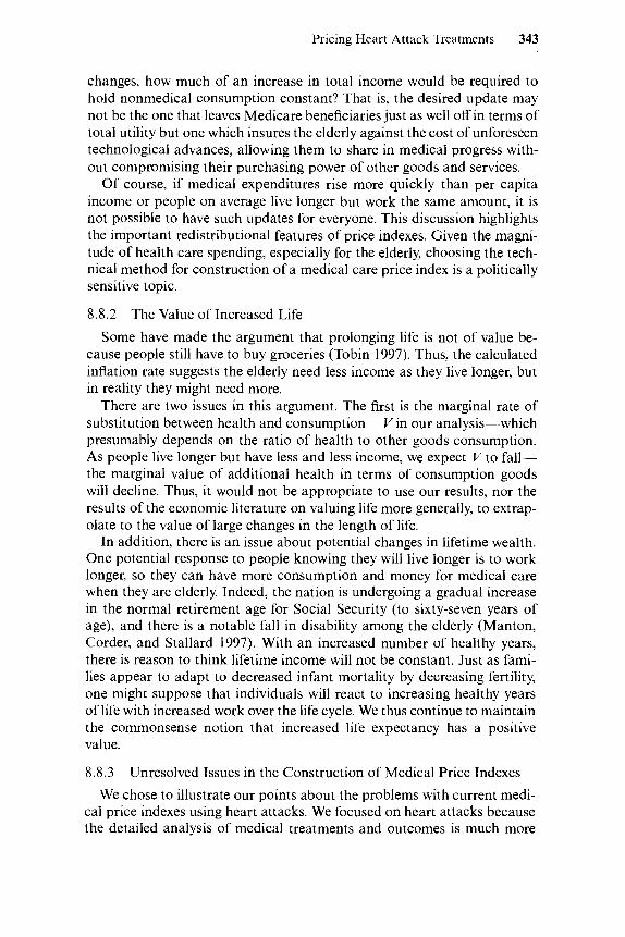
Pricing Heart Attack Treatments 343
changes, how much of an increase in total income would be required to hold nonmedical consumption constant? That is, the desired update may not be the one that leaves Medicare beneficiaries just as well off in terms of total utility but one which insures the elderly against the cost of unforeseen technological advances, allowing them to share in medical progress with- out compromising their purchasing power of other goods and services.
Of course, if medical expenditures rise more quickly than per capita income or people on average live longer but work the same amount, it is not possible to have such updates for everyone. This discussion highlights the important redistributional features of price indexes. Given the magni- tude of health care spending, especially for the elderly, choosing the tech- nical method for construction of a medical care price index is a politically sensitive topic.
8.8.2 The Value of Increased Life
Some have made the argument that prolonging life is not of value be- cause people still have to buy groceries (Tobin 1997). Thus, the calculated inflation rate suggests the elderly need less income as they live longer, but in reality they might need more.
There are two issues in this argument. The first is the marginal rate of substitution between health and consumption- V in our analysis-which presumably depends on the ratio of health to other goods consumption. As people live longer but have less and less income, we expect V to fall- the marginal value of additional health in terms of consumption goods will decline. Thus, it would not be appropriate to use our results, nor the results of the economic literature on valuing life more generally, to extrap- olate to the value of large changes in the length of life.
In addition, there is an issue about potential changes in lifetime wealth. One potential response to people knowing they will live longer is to work longer, so they can have more consumption and money for medical care when they are elderly. Indeed, the nation is undergoing a gradual increase in the normal retirement age for Social Security (to sixty-seven years of age), and there is a notable fall in disability among the elderly (Manton, Corder, and Stallard 1997). With an increased number of healthy years, there is reason to think lifetime income will not be constant. Just as fami- lies appear to adapt to decreased infant mortality by decreasing fertility, one might suppose that individuals will react to increasing healthy years of life with increased work over the life cycle. We thus continue to maintain the commonsense notion that increased life expectancy has a positive value.
8.8.3
We chose to illustrate our points about the problems with current medi- cal price indexes using heart attacks. We focused on heart attacks because the detailed analysis of medical treatments and outcomes is much more
Unresolved Issues in the Construction of Medical Price Indexes

344 D. M. Cutler, M. McClellan, J. P. Newhouse, and D. Remler
straightforward at the level of a particular disease. Heart attacks provide a particularly useful illustration because of the relative ease of measuring relevant outcomes and the substantial previous research on this condition. Nonetheless, one can ask where future work on heart attacks should go, and even more importantly how representative the findings for heart at- tacks are.
One issue is that one person’s heart attack is different from another’s and thus treatments of different individuals’ heart attacks are effectively different goods. If we are only interested in pricing an “average” heart attack and the mix was constant, this would not be a problem. However, the mix does vary. For example, if people get better at preventing heart attacks, the heart attacks actually suffered may become different in na- ture-on average a somewhat different disease. In principle, to account for changes in the mix, one could construct a “market basket” of different types of heart attacks, apply the methods presented above, and obtain an overall heart attack price index by using an appropriate set of index weights for the different types of heart attacks. But this would require even more clinically detailed analysis, and the evidence that the nature of heart attacks has not changed much in recent years suggests that such adjust- ments would not affect our conclusions very much.
A more difficult question is the extent to which our results for heart attacks are representative of price indexes for a broader range of illnesses. The representativeness of the heart attack example can be asked at two levels. One is whether the conclusion that the price increase is less than the general price index in recent years holds for other diseases. Work on the treatment of depression in the 1990s arrived at a similar conclusion (Berndt, Busch, and Frank, chap. 12 in this volume), but at present such evidence exists for few diseases.
Will it be as easy to make progress with other diseases as it was with heart attacks? There are several factors that make heart attacks a relatively easy case to study. First, they are an acute event, so that initiation of care can be dated, and a reasonable approximation to termination is also pos- sible. Second, the major procedures performed will be documented in ad- ministrative databases. Finally, mortality is a relevant outcome, though of course not the only relevant outcome.
Indeed, it is with the valuation of outcomes that the most difficult prob- lems probably lie. For example, Berndt, Busch, and Frank (chap. 12 in this volume), in estimating a price index for treating depression, considered those treatments that were therapeutically equivalent in a clinical trial to be on the same isoquant. But a substantial portion of actual treatment was off the frontier. The off-the-frontier treatment may have had no value or may have even had negative value. A full assessment of outcomes would pick up the effects of these treatments, but without studies specifically designed to do that, we are not likely to have reliable answers. Such studies

Pricing Heart Attack Treatments 345
would have to begin with a sample of patients with the disease and knowl- edge of relevant outcomes. The various dimensions of outcomes would have to be valued.
Even if heart attacks are not representative of medical care in general, forming price indexes for heart attacks highlights two issues that will be common to any medical care price index. First, our results suggest that a price index should price the treatment of a medical condition, not aparticu- Iar medical procedure. The medical procedures that are used-the number of hospital days, tests, and so on-vary over time quite dramatically. The way to integrate these changes is to look at them in the context of treating particular conditions.
Second, our results highlight the fundamental role of measuring quality in forming medical care price indexes. Incorporating quality change into the AM1 price index has a dramatic effect on our results. Because medical technology is changing so rapidly in so many areas, we suspect that mea- suring quality change in the treatment of other conditions is equally im- portant.
The Bureau of Labor Statistics has recently been improving its measure- ment of quality in medical care prices. Recently revised BLS methods at- tempt to include a quality adjustment by asking hospitals to report when major changes occurred in the treatment for the indicated condition, but we think there is a better method.24 Both the rapidity of advance in health care and the spread of managed care argue for trying to value outcomes explicitly and develop COL indexes, as we have done here. While many types of uncertainty surround outcome-based indexes, they can still pro- vide useful guidance for policy.
References
Advisory Commission to Study the Consumer Price Index. 1996. Toward a more accurate measure of the cost of living: Final report to the Senate Finance Com- mittee. Available at www.ssa.gov/history/reports/boskinrpt.html.
Armknecht, Paul A,, and Daniel H. Ginsburg. 1992. Improvements in measuring price changes in consumer services: Past, present, and future. In Output mea- surement in the service sectors, ed. Zvi Griliches. Chicago: University of Chi- cago Press.
24. Hospitals are asked to report to the BLS when treatment for the patient has materially changed, so that quality adjustments can be made. In practice, however, few hospitals do so. This may be because treatment changes are less obvious when they occur gradually as op- posed to all at once. In the case of AMI, for example, large changes in treatment over a five- or ten-year period are the cumulative effect of many modest changes in treatment; it is not obvious that hospitals could easily identify these changes as “material” and report them in any given year.

346 D. M. Cutler, M. McClellan, J. P. Newhouse, and D. Remler
Barzel, Yoram. 1968. Cost of medical treatment: Comment. American Economic Review 58 (September): 937-38.
Cardenas, Elaine M. 1996. Revision of the CPI hospital services component. Monthly Labor Review 209 (December): 40-48.
Cutler, David M., Mark McClellan, Joseph P. Newhouse, and Dahlia K. Remler. 1998. Are medical prices declining? Evidence from heart attack treatments. Quarterly Journal of Economics 113 (November): 991-1024.
Cutler. David M.. and Elizabeth Richardson. 1997. Measuring the health of the United States population. Brookings Papers on Economic A c t h y , Microeconom- ics. 217-70.
. 1998. The value of health: 1970-1990. American Economic Review 88 (2):
Fisher, Franklin M., and Zvi Griliches. 1995. Aggregate price indices, new goods, and generics. Quarterly Journal of Economics 110 (February): 229-44.
Fisher, Franklin M., and Karl Shell. 1972. The economic theory of price indices. New York: Academic Press.
Ford, Ina Kay, and Philip Sturm. 1988. CPI revision provides more accuracy in the medical care services component. Monthly Labor Review 11 1 (4): 17-26.
Fuchs, Victor. 1993. The future of health policy. Cambridge, Mass.: Harvard Uni- versity Press.
Getzen, Thomas E. 1992. Medical care price indexes: Theory, construction, and empirical analysis of the U.S. series, 1927-1990. In Advances in health economics and health services research, ed. R. M. Scheffler and L. F. Rossiter. Greenwich, Conn.: JAI Press.
Goldman, L., and E. F. Cook. 1984. The decline in ischemic heart disease mortal- ity rates: An analysis of the comparative effects of medical interventions and changes in lifestyle. Annals of Internal Medicine 101 (6): 825-36.
Griliches, Zvi, ed. 1971. Price indexes and quality change. Cambridge, Mass.: Har- vard University Press.
, ed. 1992. Output measurement in the service sectors. Chicago: University of Chicago Press.
Griliches, Zvi, and Iain Cockburn. 1994. Generics and new goods in pharmaceuti- cal price indexes. American Economic Review 84 (December): 1213-32.
Manton, Kenneth G., Larry Corder, and Eric Stallard. 1997. Chronic disability trends in the elderly United States populations: 1982-1994. Proceedings of the National Academy of Sciences 94 (6): 2593-98.
McClellan, Mark, Barbara J. McNeil, and Joseph P. Newhouse. 1994. Does more intensive treatment of acute myocardial infarction reduce mortality? Journal of the American Medical Association 272 (September): 859-66.
McGovern, P. G., J. S. Pankow, E. Shahar, K. M. Doliszny, A. R. Folsom, H. Blackburn, and R. V. Luepker. 1991. Recent trends in acute coronary heart dis- ease-Mortality, morbidity, medical care, and risk factors: The Minnesota Heart Survey Investigators. New England Journal of Medicine 334 (14): 844-90.
Moulton, Brent R., and Karin E. Moses. 1997. Addressing the quality change issue in the Consumer Price Index. Brookings Papers on Economic Activity, no. 1,
Murray, Christopher J. L., and Alan D. Lopez, eds. 1996. The global burden of disease: A comprehensive assessment of mortality and disability from diseases, in- juries, and riskfactors in 1990 andprojected to 2020. Cambridge, Mass.: Harvard University Press.
Newhouse, Joseph P. 1977. Medical care expenditures: A cross national survey. Journal of Human Resources 12 (winter): 115-25.
. 1989. Measuring medical prices and understanding their effects--the Bax-
97-100.
305-49.

Pricing Heart Attack Treatments 347
ter Prize address. Journal of Health Administration Education 7 (winter): 19-26. Newhouse, Joseph P., Shan Cretin, and Christina J. Witsberger. 1989. Predicting
hospital accounting costs. Health Care Financing Review 11 (fall): 25-33. Nordhaus, William D. 1996. Beyond the CPI: An augmented cost of living index.
Yale University, manuscript. Prospective Payment Assessment Commission. 1996. Medicare and the American
health care system: Report to the Congress. Washington, D.C.: The Commission. Scitovsky, Anne A. 1967. Changes in the costs of treatment of selected illness,
1951-67. American Economic Review 57:1182. Tobin, James. 1997. Thoughts on indexing the elderly. Public Interest Report (Fed-
eration of American Scientists) 50 (2): 13-20. Available at www.fas.org/faspir/ pir9607.html.
Tolley, George, Donald Kenkel, and Robert Fabian, eds. 1994. Valuing health for policy: An economic approach. Chicago: University of Chicago Press.
U.S. Department of Labor. Bureau of Labor Statistics. 1992. The Consumer Price Index. In BLS handbook of methods, chap. 19. Bulletin no. 2414. Washington, D.C.: Government Printing Office.
Viscusi, W. Kip. 1993. The value of risks to life and health. Journal of Economic Literuture 3 1 : 191 2-46.
Comment Frank C. Wykoff
Ever since Congress passed Medicaid and Medicare in 1965, many econo- mists and commentators have held the view that the medical treatment sector of the economy has acted like a n economic version of a physics black hole.’ The health care sector, broadly defined, seems to suck in more and more resources over time without yielding increases in output; in other words, despite huge and sustained increases in expenditures on health care over the last thirty-some years, societal indicators of health have not been improving-infant death rates, male life expectancy, proportion of citizens who have no health insurance, and the like have shown little or no im- provement. That the medical care industry is a black hole has, I believe, become conventional wisdom.
I too hold roughly this view. In fact, when asked to speak to medical groups or to the press, I have been telling them that the real crisis in Amer- ican health care is a financial problem, not a coverage problem-the prob- lem is how to prevent this sector from consuming ever larger shares of GDP without hampering the sector’s performance.2 The U.S. economy has
Frank C. Wykoff is the Eldon Smith Professor of Economics at Pomona College. 1. The black hole analogy comes from Milton Friedman (1992). Friedman freely acknowl-
edges difficulties in output measurement, but at the time, only one of the usual social indica- tors showed measurable improvement-the life expectancy of women had increased.
2. The need for federal health care reform was recognized of course in the first year of the Clinton administration. Thus President Clinton’s first term was consumed by an attempt to radically reform the financing, delivery, and provision of medical care. Unfortunately, an error in diagnosis by the Clinton team doomed their reform effort from the start. They

348 D. M. Cutler, M. McClellan, J. P. Newhouse, and D. Remler
grown at remarkable rates during the last fifty years-the 1948 U.S. econ- omy was the largest in the world in both absolute terms and in terms of the income at the median. That 1948 economy has since been multiplied about sixfold. This has not been rapid enough, though, to support growth at a constant GDP share of the medical treatment industry. The share of GDP has grown from around 7 percent to about 14 percent of GDP.3
No matter how you slice and dice the data, medical care has been a long-range fiscal disaster. Nothing else Americans spend money on- food, defense, Social Security-has grown as much as medical care.4 This problem is not unique to the United States, because while financial prob- lems are most acute in the United States, they also characterize other in- dustrial societies’ medical treatment systems, from Japan to Canada to Ge~rnany.~ All suffer the same problem-growth of medical care threatens to outstrip growth in sources of funding.
For federal government budget policy, health care is an even bigger problem. Practically nonexistent in the 1950s (less than $0.5 billion in 1955), less than a decade after Medicare passed, in 1975 total federal health care spending reached $32 billion per year. By 1995 total federal outlays for medical and health care had reached $280 billion, larger than defense, interest on the debt, and income security, an amount exceeded only by Social Security. Projections by the Congressional Budget Office based on current law, standard growth projections, and demographic trends are even scarier. By 2005, the federal government expects to spend $876 billion on health and medical care. By 2010 Medicare and Medicaid
thought the key problem was inadequate coverage of health care insurance, especially for the poor and children, when the real problem was fiscal-health care financing by the federal government was threatening to destroy the long-range federal budget equilibrium. Instead of trying to solve this fiscal problem, the Clinton reformers tried to opt for universal coverage with the same level of treatment for all recipients. This not only would have failed to solve the fiscal problem, but might have made it worse. The Clinton reform also would have re- quired radical surgery of the entire health care sector. This was a radical surgery that those in the sector fought to avoid.
Finance was the key problem, not universal coverage, because the only incremental aspect of the system was its prospective financial insolvency as a result of actuarially impossible legislative intentions written into current law, given demographic trends and the technologi- cal, diffusion, and growth dynamics of the industry. America has never had universal medical care. In fact, throughout human history, very few people have even had modern medical care, so the absence of universal care or insurance could not have been a crisis.
3. U.S. National Institutes of Health, Heulth Afuirs, fall 1994. Most of the data on federal budgets and health care spending as a portion of G D P come from the Congressional Budget Office on-line web site.
4. There is nothing inherently wrong with the medical care share of a growing G D P grow- ing, but it certainly suggests we should be getting a good deal of social gains from this sector, and the question we are raising is, Do the increases in social welfare from health care spend- ing reflect this rapid growth in medical care expenditures? Or would society be better off were we to reallocate resources away from medical care toward something else, say, child care, criminal deterrence, housing, education, or another area?
5 . Heulth Afuirs, fall 1994 contains growth rates by country that suggest all of the indus- trial societies are struggling to get a grip on medical (especially government financed) spending.

Pricing Heart Attack Treatments 349
will have surpassed Social Security in the budget. From 4 percent of GDP in 1995, federal health care spending will rise to 10 percent of GDP in 2035. Bluntly put, these medical cost growth rates, expected to run up at twice the rate of GDP, will not be sustained.
The immediate reasons, if not underlying causes, of this explosive growth of medical care expenditures are well known-an aging popula- tion; more health care per person; new, more costly technologies; and espe- cially rapid diffusion of these new technologies into standard practice. My view is that a major cause of growth in medical costs has to do with gov- ernment insurance and tax policy distortions since 1967. The argument frequently given, that technological change is a cause of rising costs, is odd.h Most industries adopt new technologies only if they raise demand or lower costs. If it is true that technology is raising costs without better products and that this, in turn, is causing medical expenditures to rise, then this signals an unhealthy industry-seriously noncompetitive and possibly a black hole.
In short, I thought the medical care industry was fiscally sick and out of control. Now along come Cutler, McClellan, Newhouse, and Remler (Cutler et al.) to tell us that the prices of heart attack treatments have not been rising but falling, that the quantity of treatments has increased and that the quality of these treatments has improved. Similar results are an- nounced for cataract surgeries and for depression treatments in other pa- pers. The theme of this conference volume seems to be that, with excep- tions like rheumatoid arthritis, medical treatments are getting much better-faster, less invasive, safer, and with better outcomes, in terms of longer life expectancy and especially in terms of improvements in post- treatment quality of life. It looks like public perceptions, or at least mine, have been wrong.
Instead of sucking up resources and releasing no improvements, medi- cal care has gotten so much better that, once properly measured, output and quality can be seen to have been rising and prices falling. Instead of carping about increased costs, budget problems, and black holes, it turns out we should be thanking the medical profession for making us so much better off. How can we (me, the public, and the statistical agencies) have been so wrong yet again?
Economists, myself included, used to worry about the productivity growth slowdown with the consequent wage stagnation grinding the econ- omy down since the early seventies. Then along came the Boskin Com- mission to tell us that statistical agencies had chronically overstated price increases, consequently understating output and productivity growth. Rather than lamenting the productivity growth slowdown, we should have been patting our leaders on the back while basking in the glory of the
6. I wish to thank Thomas Hazlett who suggested to me the possibly noneconomic impact of technology on health care efficiency.

350 D. M. Cutler, M. McClellan, J. P. Newhouse, and D. Remler
highest living standards in history. We were not falling behind the rest of the world (i.e., Japan). We were kicking some serious economic butt. Also, I was thin until a new National Institute of Health study told me I was fat. The question all these new research announcements raise is, Are the new experts right? How does one explain this evident disconnection be- tween common perceptions buttressed by previous research and official statistical indicators on the one hand and evident reality revealed by new research on the other?
Summary of the Paper
Basically, Cutler et al. argue that the traditional BLS producer and con- sumer price indexes misinterpret quantity of service increases and quality of service improvements as price increases. Thus, the official medical price indexes are biased upward. As a critique of the traditional approach, the story Cutler et al. tell is credible. Based on heart attack treatment episode cost data compiled from a (not to be identified) major teaching hospital, the authors give two reasons why medical PPI and CPI indexes are biased upward. Traditional medical price indexes indicate, as cost increases, shifts toward more expensive treatments (such as bypass surgery) and away from less expensive treatments (such as medical management). This measure- ment error is classic substitution bias resulting from fixed-weight index procedures. Correctly measured, these shifts represent increases in the quantity of treatments, thus the official indexes incorrectly partition heart attack expenditures biasing prices upward and quantities downward.
The second reason official statistics overstate increases is that insuffi- cient allowance is made for quality improvements in treatments. New treatments are better-the quality of health care has improved-because both procedures (such as angioplasty and bypass surgeries) and outcomes are better for patients. Procedures are better because downtime during treatment is less, procedures are more reliable, and pain and suffering is lower. Outcomes are better because patients live longer, and the quality of these incremental years is better because people are more ambulatory, more active, and more satisfied with the quality of their lives.
As Cutler et al. show, when proper allowance is made for shifts to better procedures, the price of heart attack treatments has been falling, not ris- ing. They conclude, “Our detailed illustrations of medical price indexes suggests, at least for the case of heart attacks, medical prices are not rising very much and may well be declining.” They aptly note that their results seem counterintuitive and ask, “Why is the public so wrong about this?” They attribute the public misperception to the above measurement error.
Critique of the Paper
As discussant, my job is to ask a different question: “Are the authors right?” And, in addition, 1 ask, “Even if they’re right, does this research
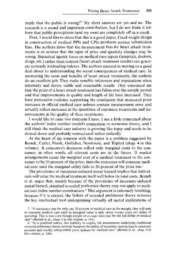
Pricing Heart Attack Treatments 351
imply that the public is wrong?” My short answers are yes and no. The research is a sound and important contribution, but I do not think it fol- lows that public perceptions (and my own) are completely off as a result.
First, I would like to stress that this is a good paper. Fixed-weight design in construction of medical PPIs and CPIs produces serious substitution bias. The authors show that the measurement bias for heart attack treat- ments is so serious that the signs of price and quantity changes may be wrong. Statistical agency focus on medical care inputs (hospitals, doctors, drugs, etc.) rather than outputs (heart attack treatment results) can gener- ate seriously misleading indexes. The authors succeed in moving us a good deal closer to understanding the social consequences of medical care. In measuring the costs and benefits of heart attack treatments, the authors do an excellent job. They make sensible inferences and imputations when necessary and derive viable and reasonable results. They convinced me that the price of a heart attack treatment has fallen over the sample period and that improvements in quality and length of life have increased. They have persuasive evidence supporting the conclusion that measured price increases in official medical care indexes contain measurement error and actually reflect increases in the quantities of expensive treatments and im- provements in the quality of these treatments.
I would like to raise two concerns I have. I am a little concerned about the authors’ index number model’s connection to economic theory, and I still think the medical care industry is growing like topsy and needs to be slowed down and probably restructured rather radically.
At the heart of my concern with the paper is a problem suggested by Berndt, Cutler, Frank, Griliches, Newhouse, and Triplett (chap. 4 in this volume). A consumer’s decisions reflect only marginal costs to the con- sumer; in other words, all relevant costs are in the future. If market arrangements cause the marginal cost of a medical treatment to the con- sumer to be 20 percent of the price, then the consumer will consume medi- cal care until the marginal utility falls to 20 percent of the price too.’
The prevalence of insurance-induced moral hazard implies that individ- uals will value the medical treatment itself well below its total costs. Berndt et al. argue that, mainly because of the prevalence of insurance-induced moral hazard, standard revealed preference theory may not apply to medi- cal care index number construction.* This argument is extremely troubling, because if it is correct, the failure of revealed preference theory removes the key intellectual tool underpinning virtually all useful implications of
7. “If consumers pay for only, say, 20 percent of medical care at the margin, they will seek to consume medical care until its marginal value is only about twenty cents per dollar of spending. This is true even though people on average must pay for the full dollar of medical care” (Berndt et al., chap. 4 in this volume, p. 145).
8. “As a practical matter, this inability to employ the assumptions underlying traditional revealed preference theory severely hampers the ability of economic statisticians to construct accurate and readily interpretable price indexes for medical care” (Berndt et al., chap. 4 in this volume, p. 146).

352 D. M. Cutler, M. McClellan, J. P. Newhouse, and D. Remler
consumer price indexes. This in turn vitiates all price and quantity parti- tions of expenditure flows related to medical care which, in turn, dimin- ishes their policy effectiveness.
Unless revealed preference theory can be employed or at least the prob- lems its absence presents finessed in some way, the economic statistician, as Berndt et al. point out, has no firm theoretical basis for contributing to the social implications of medical care. After all, without revealed prefer- ence theory, economists have very little to contribute to meaningfully mea- suring output and productivity in this sector. This charge, then, of the failure of revealed preference theory, is very damaging and needs to be addressed directly.
Cutler et al. are certainly aware of the difficulties of applying standard revealed preference theory to medical care. They argue that one cannot simply place medical services in the consumer utility function and then optimize this function subject to a budget constraint and derive price in- dexes in the usual way-that is, in their own and in Berndt et al.’s terms, they spurn revealed preference theory. I was so dismayed on being told that statistics could not be built on standard consumer optimization meth- ods that I felt economists had to abandon the field. The authors, however, moved forward and produced index numbers evidently without having to rely on consumer utility maximization (as they criticize hedonic and other approaches for doing).
How do Cutler et al. finesse the problem of constructing an index with- out any underlying utility optimization in which medical treatments ap- pear in the utility function? Well, it turns out they do this very cleverly. The problem is, I don’t think their procedure is entirely on the up-and-up.y They do build their model of treatment cost differences over time from a utility model, but the role of health care in the model is unusual and per- haps not quite kosher.
Equation (2) of Berndt et a]. and equation ( 3 ) of Cutler et al. both ex- press differences in utility between the base period without treatment and the period with treatment for the same type of utility function and for the same type of change. In particular, paring away irrelevancies, utility is derived from health which in turn depends on a medical treatment and from total expenditures on “everything else” in the consumer budget. Equating utility without treatment to utility with treatment and with less income for everything else, the authors are, in fact, imposing a first differ- ence version of a standard utility maximization exercise. Health care ex- penses and insurance costs enter the function indirectly through their effect on the ability of consumers to obtain utility from everything else.
9. My critique of the theoretical model is based on the discussion in Berndt et al. as well as on Cutler et al. From the point of view of my critique, they use the same model, even though there are some differences in details.

Pricing Heart Attack Treatments 353
The problem is that “everything else” enters the function as a value term, not a quantity, so that strictly speaking this is not a utility function, but a function in which it is already implicitly assumed that the consumer has obtained the quantity of “everything else” versus medical care treat- ment that optimizes utility. All those partial derivatives reflect someone’s margin. They do not just appear. The authors invoke Fisher and Shell (1972), but Fisher and Shell’s index number theorizing is based on con- sumer optimization. Unless the change in cost of living between utility with and without treatment, is optimal, it has no utility interpretation and is arbitrary measurement without theory. I do not see how utility or wel- fare conclusions can be derived from this model without an optimi- zation going on somewhere. Thus, I am not entirely convinced that the authors, or anyone else for that matter, can draw welfare implications from models in which no one is making rational decisions. Perhaps the eco- nomic statisticians abandon standard “revealed preference theory” at their peril.
Implications of Marginal Analysis
Actually, standard revealed preference theoryl0 can be used to analyze medical care and to partition expenditures into price and quantity compo- nents, so that one can draw social implications from price indexes, output measures, and productivity indicators. However, revealed preference the- ory does need to be applied correctly, and that is tricky for all the reasons Berndt et al. indicate. One thought for a solution is to recognize that rele- vant costs from a consumer choice, and thus a social welfare, point of view reflect only the future costs-that is, marginal costs only, not total costs incurred at the decisive moment.
Berndt et al. make this point themselves when they note that, within their model, consumption of medical care services will be valued, at the margin, by the consumer, by the marginal cost of the product. Consider the implications of this point in the following example. Utility depends on three goods, x, y, and z. The first two, x and y, are medical care treatments (cataract surgery and angioplasty) and good z is bananas. Because there
10. The authors use the phrase “standard revealed preference theory.” In my lexicon they mean standard consumer utility theory, of which revealed preference theory is one example. In equations (1) and (2) in this comment, I use marginal utility analysis. It is easy to extrapo- late from this to marginal rates of substitution by computing ratios of marginal utilities, i.e., U,lU, = MRS,, . To me, the phrase! “revealed preference theory” refers to a small piece of consumer utility theory developed by Paul Samuelson in his Foundations of Economic Anal- ysis (1963). Samuelson showed by successive experiments in which a representative consumer is faced with income-compensated alternative budget constraints that his behavior reveals his preference ordering. This is an econometric model of consumer theory. The discussions in the papers here are questioning the use of consumer theory itself, not simply Samuelson’s revealed preference version.
Despite my view that “revealed preference theory” is not “consumer utility theory,” I adopt the authors’ use of the term in this comment.
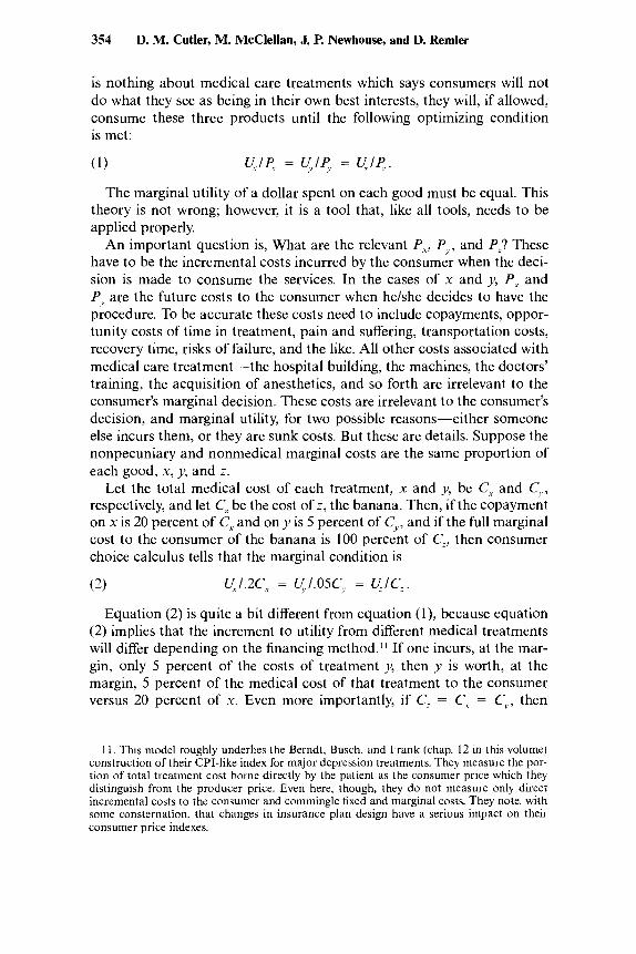
354 D. M. Cutler, M. McClellan, J. P. Newhouse, and D. Remler
is nothing about medical care treatments which says consumers will not do what they see as being in their own best interests, they will, if allowed, consume these three products until the following optimizing condition is met:
The marginal utility of a dollar spent on each good must be equal. This theory is not wrong; however, it is a tool that, like all tools, needs to be applied properly.
An important question is, What are the relevant Px, P,, and P_? These have to be the incremental costs incurred by the consumer when the deci- sion is made to consume the services. In the cases of x and y, P, and Py are the future costs to the consumer when helshe decides to have the procedure. To be accurate these costs need to include copayments, oppor- tunity costs of time in treatment, pain and suffering, transportation costs, recovery time, risks of failure, and the like. All other costs associated with medical care treatment-the hospital building, the machines, the doctors’ training, the acquisition of anesthetics, and so forth are irrelevant to the consumer’s marginal decision. These costs are irrelevant to the consumer’s decision, and marginal utility, for two possible reasons-either someone else incurs them, or they are sunk costs. But these are details. Suppose the nonpecuniary and nonmedical marginal costs are the same proportion of each good, x, y, and z .
Let the total medical cost of each treatment, x and y, be C, and Cy, respectively, and let Cz be the cost of z , the banana. Then, if the copayment on x is 20 percent of C, and on y is 5 percent of C,, and if the full marginal cost to the consumer of the banana is 100 percent of Cz, then consumer choice calculus tells that the marginal condition is
(2) ql.2C.y = V,/.05C, = YIC,
Equation (2) is quite a bit different from equation (l), because equation (2) implies that the increment to utility from different medical treatments will differ depending on the financing method.” If one incurs, at the mar- gin, only 5 percent of the costs of treatment y, then y is worth, at the margin, 5 percent of the medical cost of that treatment to the consumer versus 20 percent of x. Even more importantly, if C, = C, = C,,, then
1 1 . This model roughly underlies the Berndt, Busch, and Frank (chap. 12 in this volume) construction of their CPI-like index for major depression treatments. They measure the por- tion of total treatment cost borne directly by the patient as the consumer price which they distinguish from the producer price. Even here, though, they do not measure only direct incremental costs to the consumer and commingle fixed and marginal costs. They note, with some consternation, that changes in insurance plan design have a serious impact on their consumer price indexes.

Pricing Heart Attack Treatments 355
consumers value some medical treatments at 5 percent and some medical treatments at 20 percent of a banana! Suppose further that the total costs of these three items, x, y, and z reflect social costs, then this analysis sug- gests that very large social costs, in the form of valuable resources, are being used up by the medical treatment sector for which consumers are getting back very little utility.’* This sure sounds like an economic version of a black hole to me!
An Enigma Suggests a New Perspective
There remains an enigma with marginal analysis of the industry which suggests that something is missing. If consumers only value medical care at the margin equal to the copayment, then how does society justify all these fixed costs associated with the treatment? The utility, at least in some sense, of medical care must exceed the marginal cost of the treatment. Otherwise, society chronically spends way too much on medical care. Put another way, if the only social welfare from medical care is based on the marginal utility to the patient from the treatments, then why does society persist in spending so much more for medical care than can be justified by these 10 percent or 30 percent copayments? Is such a major nonmarket (government or nonprofit sector) failure likely? Should we cut medical care sector spending back to 10 to 30 percent of its current size? Would refi- nancing techniques, like medical IRAs, designed to shift more costs in- curred by the patient to the future, cause a radical decline in the social costs of medical care? In short, do we need to neutralize this black hole before it sucks us financially dry?
Maybe, but maybe not. Obviously, this policy issue has something to do with insurance and its resultant moral hazard and principal agent prob- lems noted by Berndt et al. and with the role of the government and non- profit organizations. Is this a case of poor policy design based on poor policy analysis of the nonprofit and public sectors, which has ignored mod- ern public choice theory, and in so doing has allowed this industry to grow like topsy? All of this may be true, but is it?
One possible out can be found in Philipson and Lakdawalla (chap. 3 in this volume) on nonprofit sector conduct. The Philipson and Lakdawalla model suggests that utility from medical care services is enjoyed by eco- nomic agents other than the patient. The authors argue that donors to nonprofits obtain utility from both medical care output and from medical care input. If so, then society, in some large sense, may be providing wel- fare from medical care beyond that enjoyed by the patient. This model is suggestive, but, according to Richard Frank’s critique, still has some way to go before we can accept it as viable.
12. All of this analysis can be done with marginal rates of substitution or with Samuelson’s revealed preference model, but the above approach makes the points more clearly.

356 D. M. Cutler, M. McClellan, J. P. Newhouse, and D. Remler
I would like to suggest a different way of looking at the problem. I sug- gest a model which regrounds medical price indexes on standard economic theory, partially reconciles this evident social failure, and suggests some different directions for new research. Let us take a tip from Jack Triplett’s notion that human bodies, like cars or other machines, require mainte- nance and repair, and that there are many parallels between the two indus- tries. Like Triplett, I am not so crass as to suggest humans are machines, but, also like Triplett, I believe one can gain insight into medical care by looking at how economic statisticians price automobile repair. * ?
I shall build on Triplett by beginning with Zvi Griliches’s critique of the Triplett paper, in which Griliches points out that economic statisticians evidently do not construct very good indexes of car repair either.I4 Produc- tivity growth figures for the automobile repair industry, compiled by Gril- iches from official statistics, imply negative average annual productivity growth. Negative productivity growth, in Griliches’s judgment, is not cred- ible. It fails what Chuck Hulten (1990) calls the “interocular test”-the error is so large that it hits you right between the eyes. While Griliches’s point that car repair indexes are seriously flawed is persuasive, rather than answering a question it begs one-Why do we construct such poor auto- mobile repair indexes? Just as we might learn about medical care by seeing what we do right elsewhere, perhaps errors we make in measuring car re- pair index design can tip us off to what is wrong with health care mea- surement.
I think we need to apply capital theory carefully to both car repair and to health care. One way to do this in the health care case is to reinterpret insurance policies as acquisition of capital assets by the insured. The capi- tal asset purchased can be viewed as an ownership right in a medical-care- industry (mc) asset. This mc asset is capable of generating various services, treatments, diagnostic tests, service inspections, tune-ups, and so forth. In other words, suppose consumers view an insurance contract as purchasing ownership rights to an asset with known properties. These known proper- ties consist of reasonable access in the future to medical care (under the terms of the insurance contract).
While, from an insurance company’s point of view, an insurance con- tract may be a contingent contract for a service that may or may not be
13. Triplett points out, in chapter 1 of this volume, that many of the problems analysts normally think are unique to medical care are also encountered in the automobile repair industry. Asymmetric information, stochastic demands, principal agent problems, and moral hazard under insurance all occur in the automobile industry as well. The only real difference seems to be that one can trade in old cars for new models, but the old body has to last until death. With organ transplants and genetic engineering, even this distinction may soon dis- appear.
14. Griliches, in his comment to chapter 1 in this volume, shows that the productivity growth figures for medical care and for automobile repair have both been negative in recent years. Do we really think that with all the new diagnostic methods available in both areas efficiency and economic performance have declined?

Pricing Heart Attack Treatments 357
needed at some future time, with the resultant moral hazard problem of overconsumption, this view may not represent the consumer’s perspective, and after all we certainly ought to take the consumer’s perspective in de- signing a consumer price index. Building on capital theory, assume that the consumer views his insurance premiums as buying ownership rights to an mc asset. This mc asset can be thought of as ownership in a “firm” that produces a flow of medical services available to the owner when he or she chooses to use them.15 The service flow that derives from the asset is analogous to the service flow from any other asset or, if you will, machine (or, a la Triplett, car).
From Jorgenson’s model of capital theory,I6 competitive equilibrium im- plies that the acquisition price of a new asset in period t , q(0, t ) , equals the present discounted value of the future flow of user costs of capital on the asset over the life of the asset. so that
(3)
where s indexes time and where L is the life of the asset.” Note that the cost of using the asset in period t + s is c(s, t + s), the cost of the period t + s flow of services, not q(0, t ) nor q(0, t + s). At acquisition, given either perfect foresight or rational expectations, the asset price paid for the insurance, the present discounted value of the premium stream, must equal q(0, t ) and therefore this asset price represents the marginal utility to the consumer of buying that asset in period t .
Now one may argue that because health care is financed through work, the market is noncompetitive. This may be partly so. Certainly, we all know that the tax system biases these prices. One may also argue, as Phil- ipson and Lakdawalla do, that since the industry is nonprofit, normal com- petitive conditions do not explain production. But beyond these distor- tions, the assumption that competitive forces work on health insurance packages available to and acquired by workers seems pretty good. After all, workers can change jobs; they can change health plans; they do have periodic choices. Thus, I, for one, am comfortable with the assumption that after allowing for tax policy distortions, the cost of insurance repre- sents the utility the payer associates with the present value of access to the future flow of medical care services.’*
15. The owner here is a producer who uses the asset to produce health; or, more precisely, uses the flow of services from the mc asset to maintain his human capital asset producing at some optimal level. This producer is, of course, the same person as the consumerlworkerl humanhnsured.
16. See, for example, Jorgenson (1 973), Hulten (1 990), and Wykoff (1998). 17. Strictly speaking s indexes age and t + s date, because with machines age of the asset
matters. We discuss the meaning of s in the case of an mc asset below. 18. The utility and welfare implications of Medicare insurance and other government pro-
grams are different. One may want to build a model directly on a societal welfare function rathcr than from a consumer utility model. 1 ignore this issue in this comment.

358 D. M. Cutler, M. McCiellan, J. P. Newhouse, and D. Remler
Leaving aside copayments for the moment, suppose the entire cost of medical care is covered by insurance companies (from premiums) with whom the members of the HMO (or health plan) are insured. If we com- pute the asset price q(0, t ) of the insurance contracts, then the marginal utility to the representative health care consumer of period t + s health care, in equilibrium, must equal the user cost of capital c(s, t + s) from equation (3).19 If this were not so, then the consumer/worker would change assets; in other words, he would sell this contract and buy another one.
Put another way, optimizing economic agents, on the buyer’s side of the medical care industry, purchase assets at prices that reflect the marginal utility they associate with the assets. This means that the “marginal utility” of medical care, when the insurance is purchased, is the product of the price of the insurance asset times the number of consumers who purchase these assets. The sum over the patient population of these expenditures covers the cost of producing medical care, including the cost of financing it. Thus, the relevant price index, from the consumer’s point of view, for any one period, is simply that period’s user cost of the mc asset.
All that remains to be done is compute the user cost. That is, one needs to spread the acquisition cost of the asset over its life into period-by-period components. This has been done with machines and human capital by Jorgenson and Associates (see, e.g., Lau 2000) by defining the efficiency function, +(s), which indicates the in-use productive efficiency of an asset age s relative to the efficiency of a new asset. The meaning of age-based efficiency for an ownership right in a medical care asset is different from efficiency by age of machines. In general, though, the + function can take many possible forms anyway. It need not even be a function, but can be a sequence. One can normalize +(s) on a new asset, so that +(0) = 1. For machines, which depreciate, + is then a nonincreasing function like
s = 1 2 3 4 . . .
+(s) = 1 .9 .8 .6 . . . .
The efficiency function of an mc asset need not be nonincreasing. In fact, with health care, it is important to note that efficiency will change with technological change, and this suggests an important research topic for the future. In the absence of technological change, though, perhaps the mc asset +(s) is the same for all s. Such a machine is called a one-horse- shay asset in the capital theory literature.
19. I am assuming away here problems associated with coercion in forcing workers to choose from a limited list of possible health care plans, so that the market for choice is thick enough that the representative health care consumer can buy what he or she wants. In fact, this model suggests why disputes occur over the packages offered by various employers-- these disputes may simply reflect consumer demands to include their optimal asset package in their set of options.

Pricing Heart Attack Treatments 359
Using the concept of an efficiency function here for this medical care asset, and, assuming competitiveness in the asset market, we can simplify equation (3):
s=L +( s)c(O, t ) s=o (1 + r ) S
4 i Q t ) = c Now allocating insurance costs over the life of the plan member or pa-
tient boils down to determining acquisition cost of the insurance contract and the form of the efficiency function. As a first approximation, this ap- proach will produce a more accurate measure of the price/quantity parti- tion of medical costs than either pricing hospitals, which is current official practice, or treatments, which is suggested by the paper under review as well as by others in this volume.
A natural objection to this asset approach is that it does not account for the stochastic use of the health care asset or what is the same thing for differences in use patterns over the life of the asset. However, that is exactly the point of this exercise. Measuring the cost of specific treatment events or the cost of hospitals and medical personnel both miss the main point of the medical care product from the consumer’s point of view. This be- comes clear when one considers the machine analogue. Suppose a con- sumer buys a telephone, and economic statisticians want to know the utility derived from the phone by the consumer. Economic statisticians usually do one of two things. They price phones and construct indexes on phone production. Or they allocate this asset acquisition price over the life of the phone and build an index on the user cost. The latter approach is clearly more accurate for measuring consumption of phone services per period than the former, and this point is the essence of the Jorgenson user- cost contribution to production theory and measurement.2o
But neither approach tries to dig into the issue of when exactly owners are using the phone. Do you only use your phone when you talk on it? Do you only use it when you get a call? No. That asset is providing you a flow of services, just like your desk, chair, and car, all the time. It makes little sense to only place utility on your phone or chair when you are talking or sitting. In fact, ownership of assets generally provides two types of ser- vice flows: a “passive flow” by being there when and if needed-to re- ceive calls, to be sat in, to be ready for workers to employ-and an “active flow”-driving it, drilling with it, sitting on it.*l
This is not to say that the question of when you actually consume or
20. Copayments may be integrated into the model, but will require distinguishing between those one expects to incur and those that come as surprises. This distinction is discussed below.
21. The idea that service flows from assets may consist of more than active use comes from Charles R. Hulten (1990), though he bears no fault for my use of the idea here.

360 D. M. Cutler, M. McClellan, J. P. Newhouse, and D. Remler
produce “active services” with an asset, whether it be health care or cars or phones, is uninteresting. It is to say that this is not the only use one gets from the asset. Furthermore, this suggests to me that approaching the problem of measuring social valuations of health care by trying to measure these “active services” or treatment costs alone is going to give the wrong answer.22 The economic statistician will accurately value the phone only if utility from the phone derives solely from actual calls.
This capital theory focus suggests a line of research that needs to be developed both for understanding asset use and for understanding issues like maintenance and repair of cars and provision of health care. How do we disentangle the value of the asset and its future flow of user costs for the entire asset including the “passive services” from the “active services” measures, such as treatment costs and their marginal valuations? This will not be easy to do, which is probably why it has not yet been done.
To begin thinking about what it means to use an asset, and to maintain and repair it, requires, I think, modeling expected and unexpected uses of the active service. No one buys a machine or car expecting it to be an infinitely lived one-horse-shay and no one expects an infinite life span with perfect health. (We may pray for this, but we do not expect it.) Owners of both machines and humans (ourselves) expect these assets to incur down- times, to require maintenance and repair, and to have finite lives. The lengths of these lives also are uncertain in both cases.
This approach suggests that rational economic agents fully expect a sto- chastic stream of care in order to maintain the output service flow from capital assets, whether human or not. In each case, then, one can acquire an a priori contract to provide, under predictable cost conditions, the nec- essary maintenance and repairs. Owners in both cases also can (usually) decide they would rather not pay to acquire the contracts or insurance policies to cover future stochastic maintenance and repair events, and simply pay as they From an indexing point of view, of course, the lat- ter financing option is easy for the economic statistician to deal with. The former is what is giving us fits. But the former is easier if one simply views the contract insurance policy to cover the utility to the consumer of access to the medical care asset when needed, knowing that it will be needed, but not exactly when. In other words, the full price of the contract for the patient groups under private insurance covers the entire expected future flow of medical care services. Only unexpected events need to be ac- counted for in addition.
Measurement problems occur when reality diverges from expectations, even if both are stochastic. In general, though, I would argue that most
22. See Berndt and Fuss (1986) for an interesting perspective on capital utilization. 23. Under perfect foresight or rational expectations, copayments as well as premiums can
be integrated into q(0, t ) by appropriately discounting these expenses to time t .

Pricing Heart Attack Treatments 361
insurance costs cover expected treatment flows. Two kinds of unanticipat- able deviations present problems. These would be events that are so rare that economic agents cannot be expected to form probabilities of their o c c ~ r r e n c e . ~ ~ One type of unexpected change is environmental shocks and surprising changes in the demographic composition of the patient group- climate warming and depletion of the ozone layer or hard-to-predict in- creases in life spans and changes in conduct while living can all radically alter health care costs.25 Earthquakes, hurricanes, tornadoes, and the like can be expected to occur with some probability, so they are covered. Nor- mal population growth, though not war-related baby booms, can be ex- pected. Normal day-to-day activities and accidents can be expected. It is only inexplicable deviations from normal that cannot easily be subsumed under some probabilistic contractual basis.
The other true surprises are unexpected jumps in technology which alter the relationship between the present value of premiums and the present value of the costs of supplying the medical care asset. As in the cases of environment and demographics, some stream of technological change can be expected, but not sudden large jumps-such a sudden jump might be the discovery of Viagra, a unexpected new impotence treatment that is na- turally very much in demand.26 More typical, in recent years, is that new expensive treatments become available and are rapidly diffused into popu- lar use. HMO insurance contracts tend to promise “standard practice” treatment. As a practical matter, standard practice changes over the course of the insurance ~ontract .~’ Does the promise of standard practice care mean that HMOs and patients are willing to accommodate any and all technological shocks? No.
In recent years, the notion of standard practice treatment may have got- ten both buyers and sellers into trouble, because very expensive treatments are rapidly diffused into becoming standard practice, even though both sides of the market may want to avoid new costly procedures.2s Thus, in- surance contracts are being regularly renegotiated to reflect the very rap- idly changing technology. This recontracting and rapid technological change issues can be integrated into the capital theory approach, but that is another subject for future research.
24. Keynes (1935) draws this distinction in his analysis of liquidity preference. 25. Food supplement advertisements targeted at aged populations suggest that older
people take up scuba diving and other risky activities. If older people undertake risky activi- ties, then the accident rate and incidence of active service flow from the medical care asset could rise.
26. Kaiser Permanente, a major HMO, announced in June 1998, as this is being written, that if it were to cover Viagra, it would become insolvent.
27. HMOs will provide new treatments to avoid litigation and negative press. They do not want to deny care, because they fear adverse reputation effects which lower the value of the firm.
28. This problem is especially acute when new discoveries result in very expensive treat- ments that are then used for patients whose conditions are not medically suitable.

362 D. M. Cutler, M. McClellan, J. P. Newhouse, and D. Rernler
I want to repeat that the paper by Cutler et al. is a very exciting piece of research into a problem of major social concern. The authors have taken on a difficult task and succeeded in stimulating a good deal of think- ing about this very important issue.
References
Berndt, Ernst R., and Melvyn A. Fuss. 1986. Productivity measurement with ad- justments for variations in capacity utilization, and other forms of temporary equilibrium. Journal of Econometrics 33:7-29.
Fisher, Franklin M., and Karl Shell. 1972. The economic theory of price indexes. New York: Academic.
Friedman, Milton. 1992. Input and output in medical care. Stanford, Calif.: Hoover Institution, Stanford University.
Hulten, Charles R. 1990. The measurement of capital. In Fifty years of economic measurement: The jubilee of the Conjerence on Research in Income and Wealth, ed. Ernst R. Berndt and Jack E. Triplett. NBER Studies in Income and Wealth, vol. 54. Chicago: University of Chicago Press.
Jorgenson, Dale W. 1973. The economic theory of replacement and depreciation. In Econometrics and economic theory: Essays in honor of W Sellykraerts. New York: Macmillan.
Keynes, John Maynard. 1935. The general theory of employment, interest, and money. New York: Harcourt, Brace and World.
Lau, Lawrence J., ed. 2000. Econometrics and the cost of capital: Essays in honor of Dale W Jorgenson. Econometrics, vol. 2. Cambridge, Mass.: MIT Press.
Samuelson, Paul A. 1963. Foundations of economic analysis. Cambridge, Mass.: Harvard University Press.
US. National Institutes of Health. 1994. Health Afsairs, fall. Wykoff, Frank C. 1998. Comment on Barbara Fraumeni, “Expanding economic
accounts for productivity analysis: A nonmarket and human capital perspec- tive.” Paper presented at NBER CRIW conference on New Directions in Pro- ductivity Research, Silver Spring, Md., April.