Pricing Derivatives with Barriers

in a Stochastic Interest Rate Environment

Carole Bernard (University of Waterloo)

Olivier Le Courtois (E.M. Lyon)

François Quittard-Pinon (University of Lyon)

1

Introduction

Our aim : pricing barrier products

when interest rates are stochastic.

In order to illustrate our methodology,

we study a particular barrier option : the Shark Option.

Yet, our approach is very general,

and has applications in lots of other fields.

2

Relevance

26% of Equity Linked Products currently traded on the

American Stock Exchange are Barrier Products.

Applications : Extension of Rubinstein and Reiner (1991)

Formulas for Barrier Options, Defaultable Bonds,

Structured Products, Index Linked Derivatives,

Real Options, Stock Options, Portfolio Allocation

Market Value of Life Insurance Contracts.

Maturity of traded barrier products can be quite long,

up to 5 years (among Index Linked Notes).

⇒ Stochastic Interest Rates.

3

Outline of the Talk

➠ Description of the Shark Option

➠ Underlying and Interest Rate Model

➠ Two Types of Barriers :

1. Constant Barrier

2. Stochastic Barrier

⇒ Two Valuation Methods

➠ Numerical Analysis

4

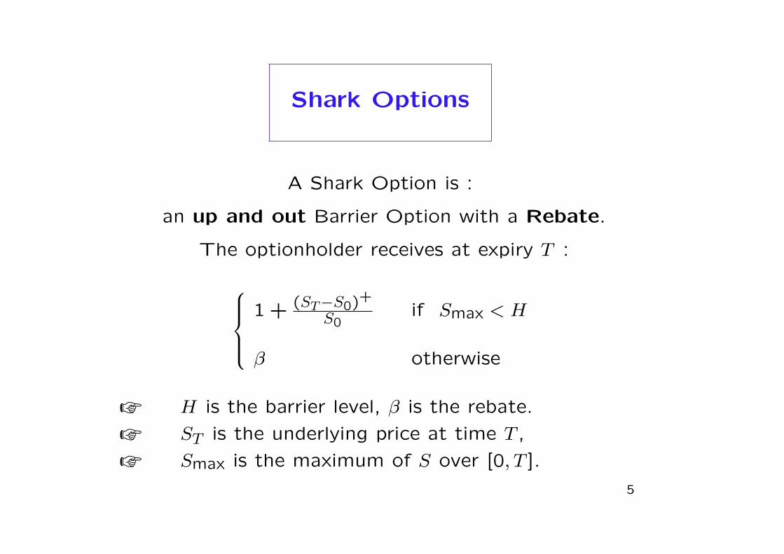
Shark Options

A Shark Option is :

an up and out Barrier Option with a Rebate.

The optionholder receives at expiry T :

1 + (ST−S0)+

S0if Smax < H

β otherwise

☞ H is the barrier level, β is the rebate.

☞ ST is the underlying price at time T ,

☞ Smax is the maximum of S over [0, T ].

5

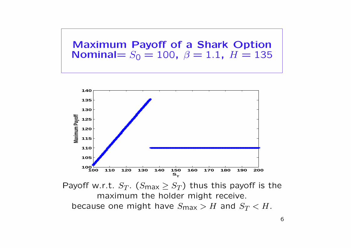
Maximum Payoff of a Shark OptionNominal= S0 = 100, β = 1.1, H = 135

100 110 120 130 140 150 160 170 180 190 200100

105

110

115

120

125

130

135

140

ST

Maxim

um Pa

yoff

Payoff w.r.t. ST . (Smax ≥ ST ) thus this payoff is the

maximum the holder might receive.

because one might have Smax > H and ST < H.

6

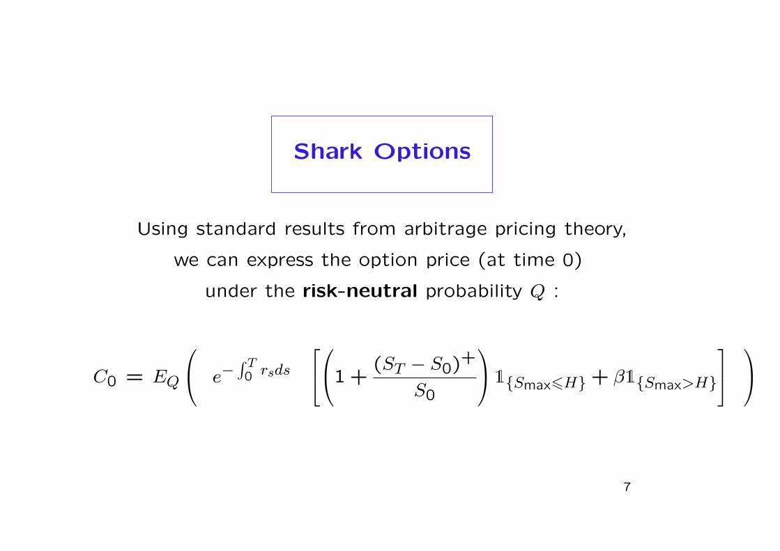
Shark Options

Using standard results from arbitrage pricing theory,

we can express the option price (at time 0)

under the risk-neutral probability Q :

C0 = EQ

e−∫ T0 rsds

1 +(ST − S0)

+

S0

1{Smax6H} + β1{Smax>H}

7

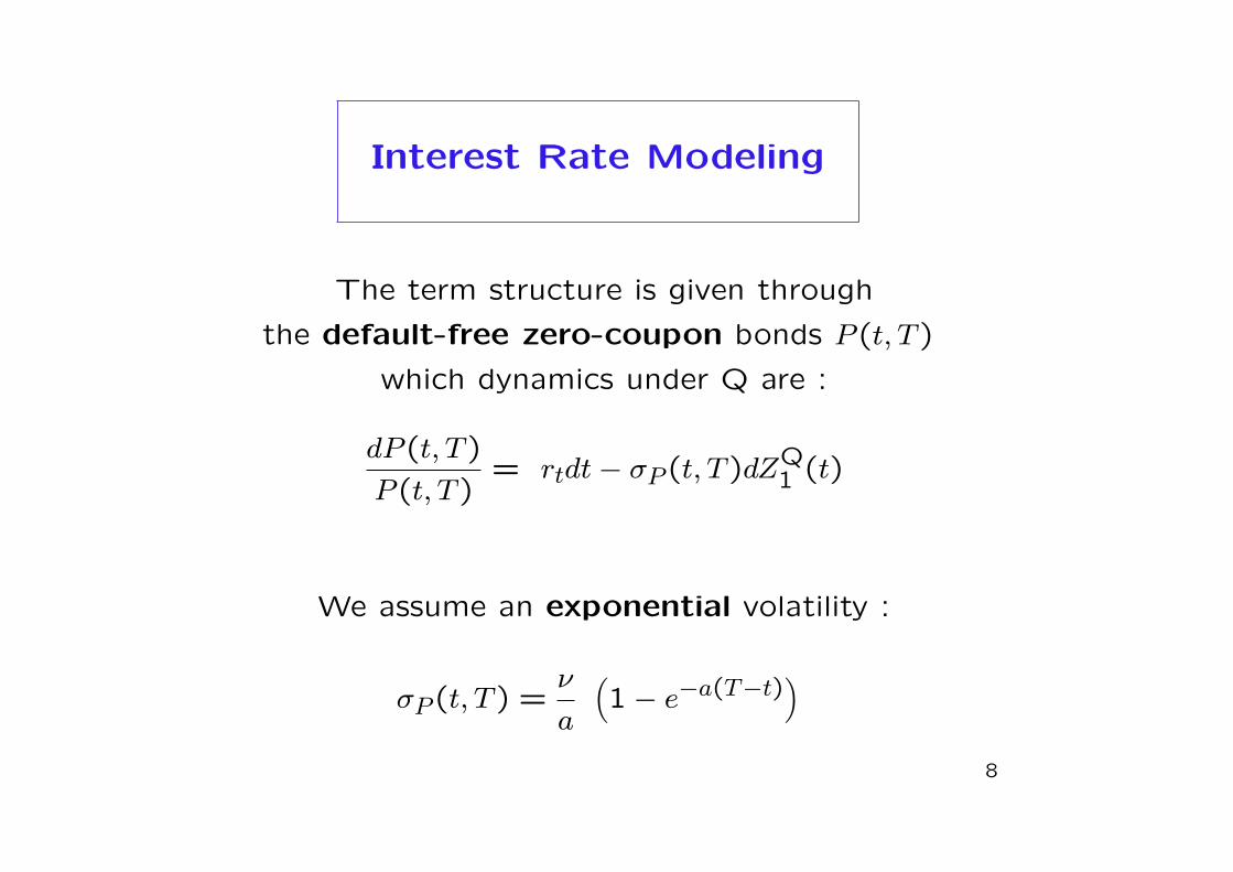
Interest Rate Modeling

The term structure is given through

the default-free zero-coupon bonds P (t, T )

which dynamics under Q are :

dP (t, T )

P (t, T )= rtdt − σP (t, T )dZQ

1 (t)

We assume an exponential volatility :

σP (t, T ) =ν

a

(1 − e−a(T−t)

)

8

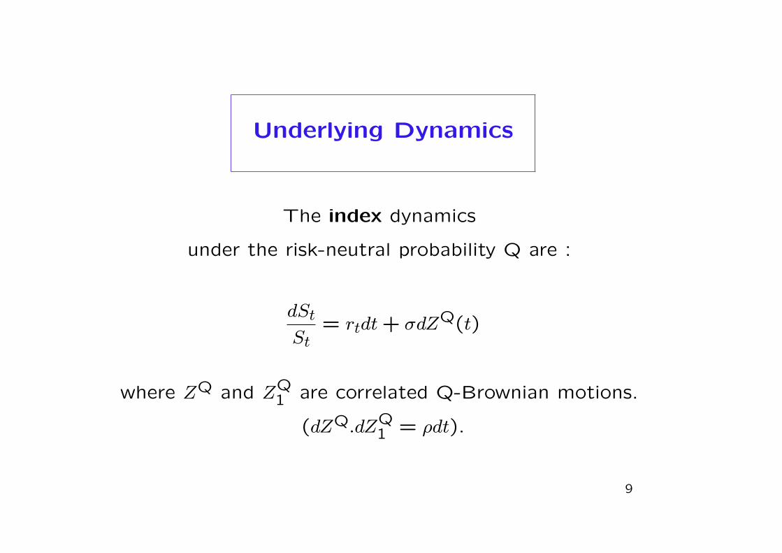
Underlying Dynamics

The index dynamics

under the risk-neutral probability Q are :

dSt

St= rtdt + σdZQ(t)

where ZQ and ZQ1 are correlated Q-Brownian motions.

(dZQ.dZQ1 = ρdt).

9

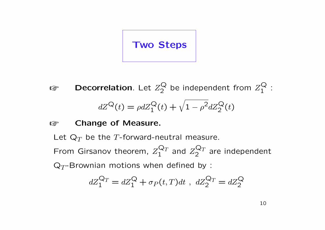
Two Steps

☞ Decorrelation. Let ZQ2 be independent from ZQ

1 :

dZQ(t) = ρdZQ1 (t) +

√1 − ρ2dZQ

2 (t)

☞ Change of Measure.

Let QT be the T -forward-neutral measure.

From Girsanov theorem, ZQT1 and Z

QT2 are independent

QT -Brownian motions when defined by :

dZQT1 = dZQ

1 + σP (t, T )dt , dZQT2 = dZQ

2

10

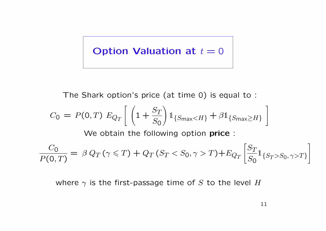
Option Valuation at t = 0

The Shark option’s price (at time 0) is equal to :

C0 = P (0, T ) EQT

[ (

1 +ST

S0

)

1{Smax<H} + β1{Smax≥H}

]

We obtain the following option price :

C0

P (0, T )= β QT (γ 6 T ) + QT (ST < S0, γ > T )+EQT

[ST

S01{ST>S0, γ>T}

]

where γ is the first-passage time of S to the level H

11

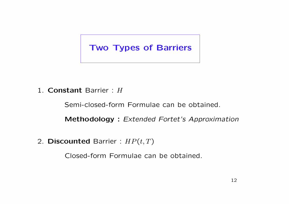
Two Types of Barriers

1. Constant Barrier : H

Semi-closed-form Formulae can be obtained.

Methodology : Extended Fortet’s Approximation

2. Discounted Barrier : HP (t, T )

Closed-form Formulae can be obtained.

12

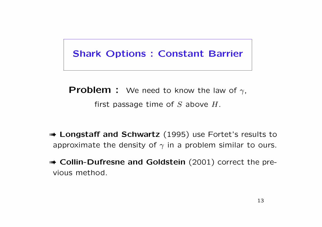
Shark Options : Constant Barrier

Problem : We need to know the law of γ,

first passage time of S above H.

➠ Longstaff and Schwartz (1995) use Fortet’s results to

approximate the density of γ in a problem similar to ours.

➠ Collin-Dufresne and Goldstein (2001) correct the pre-

vious method.

13

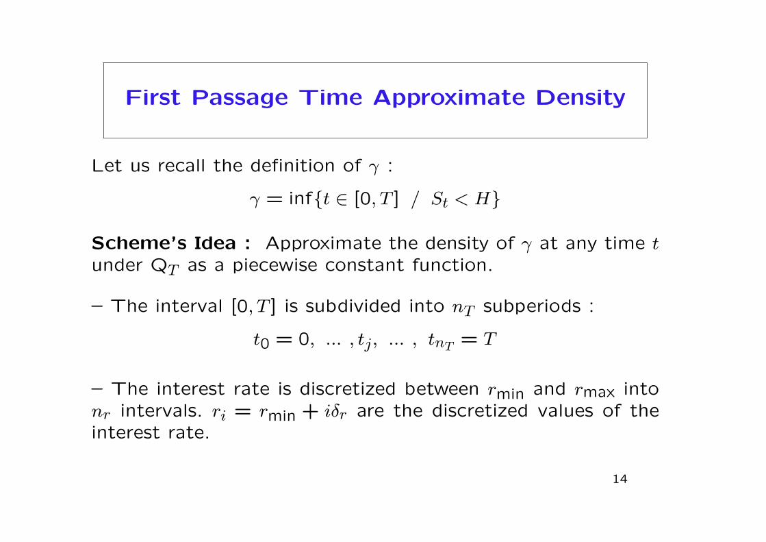
First Passage Time Approximate Density

Let us recall the definition of γ :

γ = inf{t ∈ [0, T ] / St < H}

Scheme’s Idea : Approximate the density of γ at any time tunder QT as a piecewise constant function.

– The interval [0, T ] is subdivided into nT subperiods :

t0 = 0, ... , tj, ... , tnT = T

– The interest rate is discretized between rmin and rmax intonr intervals. ri = rmin + iδr are the discretized values of theinterest rate.

14

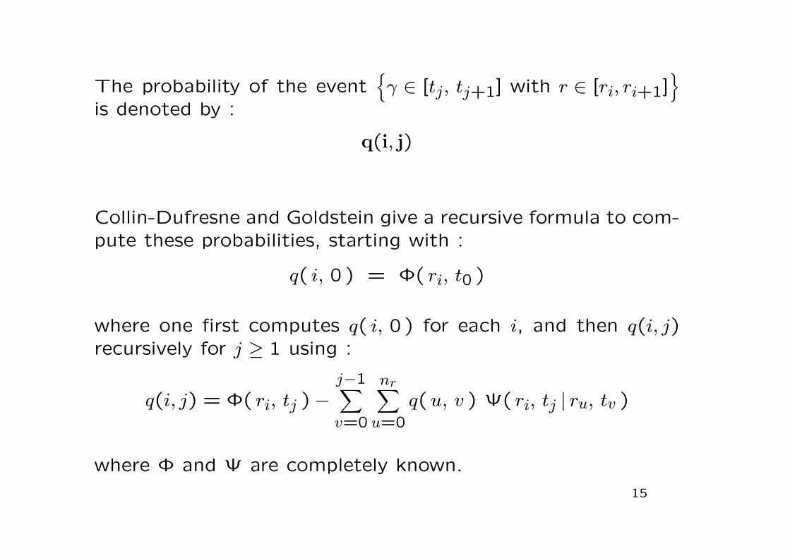
The probability of the event{γ ∈ [tj, tj+1] with r ∈ [ri, ri+1]

}

is denoted by :

q(i, j)

Collin-Dufresne and Goldstein give a recursive formula to com-

pute these probabilities, starting with :

q( i, 0 ) = Φ( ri, t0 )

where one first computes q( i, 0 ) for each i, and then q(i, j)recursively for j ≥ 1 using :

q(i, j) = Φ( ri, tj ) −j−1∑

v=0

nr∑

u=0

q(u, v ) Ψ( ri, tj | ru, tv )

where Φ and Ψ are completely known.

15

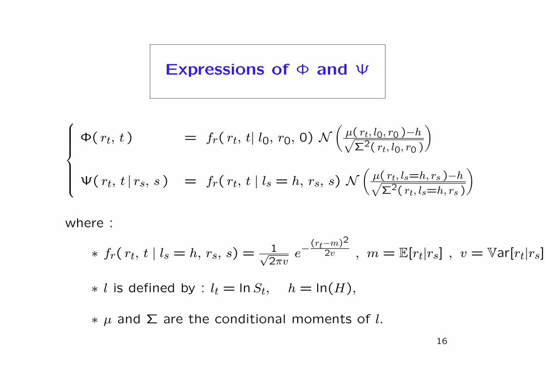
Expressions of Φ and Ψ

Φ( rt, t ) = fr( rt, t| l0, r0, 0) N(

µ( rt, l0, r0 )−h√Σ2( rt, l0, r0 )

)

Ψ( rt, t | rs, s ) = fr( rt, t | ls = h, rs, s) N(

µ( rt, ls=h, rs )−h√Σ2( rt, ls=h, rs )

)

where :

∗ fr( rt, t | ls = h, rs, s) = 1√2πv

e−(rt−m)2

2v , m = E[rt|rs] , v = Var[rt|rs]

∗ l is defined by : lt = lnSt, h = ln(H),

∗ µ and Σ are the conditional moments of l.

16

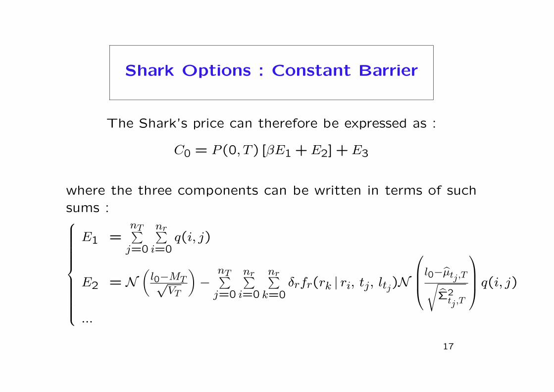
Shark Options : Constant Barrier

The Shark’s price can therefore be expressed as :

C0 = P (0, T ) [βE1 + E2] + E3

where the three components can be written in terms of such

sums :

E1 =nT∑

j=0

nr∑

i=0q(i, j)

E2 = N(

l0−MT√VT

)−

nT∑

j=0

nr∑

i=0

nr∑

k=0δrfr(rk | ri, tj, ltj)N

l0−µ̂tj,T√

Σ̂2tj,T

q(i, j)

...

17

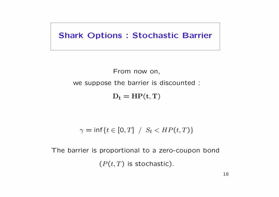
Shark Options : Stochastic Barrier

From now on,

we suppose the barrier is discounted :

Dt = HP(t,T)

γ = inf{t ∈ [0, T ] / St < HP (t, T )}

The barrier is proportional to a zero-coupon bond

(P (t, T ) is stochastic).

18

Shark Options : Discounted Barrier

We use time change techniques

in a similar way as Briys and de Varenne [1997]

who extended the Black and Cox model [1976]

by considering a stochastic default barrier.

and the following well-known Tools :

- Girsanov Theorem

- Dubins-Schwarz Theorem

19

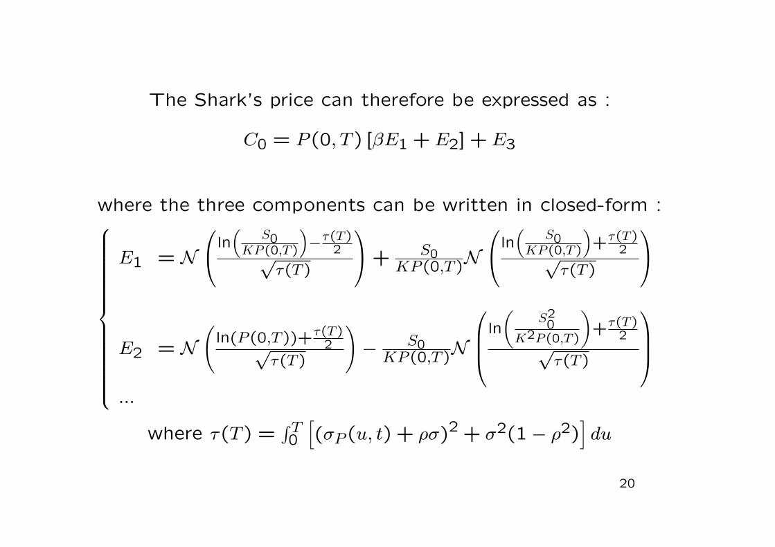
The Shark’s price can therefore be expressed as :

C0 = P (0, T ) [βE1 + E2] + E3

where the three components can be written in closed-form :

E1 = N

ln(

S0KP (0,T )

)−τ(T )

2√τ(T )

+ S0KP (0,T )

N

ln(

S0KP (0,T )

)+

τ(T )2√

τ(T )

E2 = N(

ln(P (0,T ))+τ(T )

2√τ(T )

)

− S0KP (0,T )

N

ln

(S20

K2P (0,T )

)+τ(T )

2√τ(T )

...

where τ(T ) =∫ T0

[(σP (u, t) + ρσ)2 + σ2(1 − ρ2)

]du

20

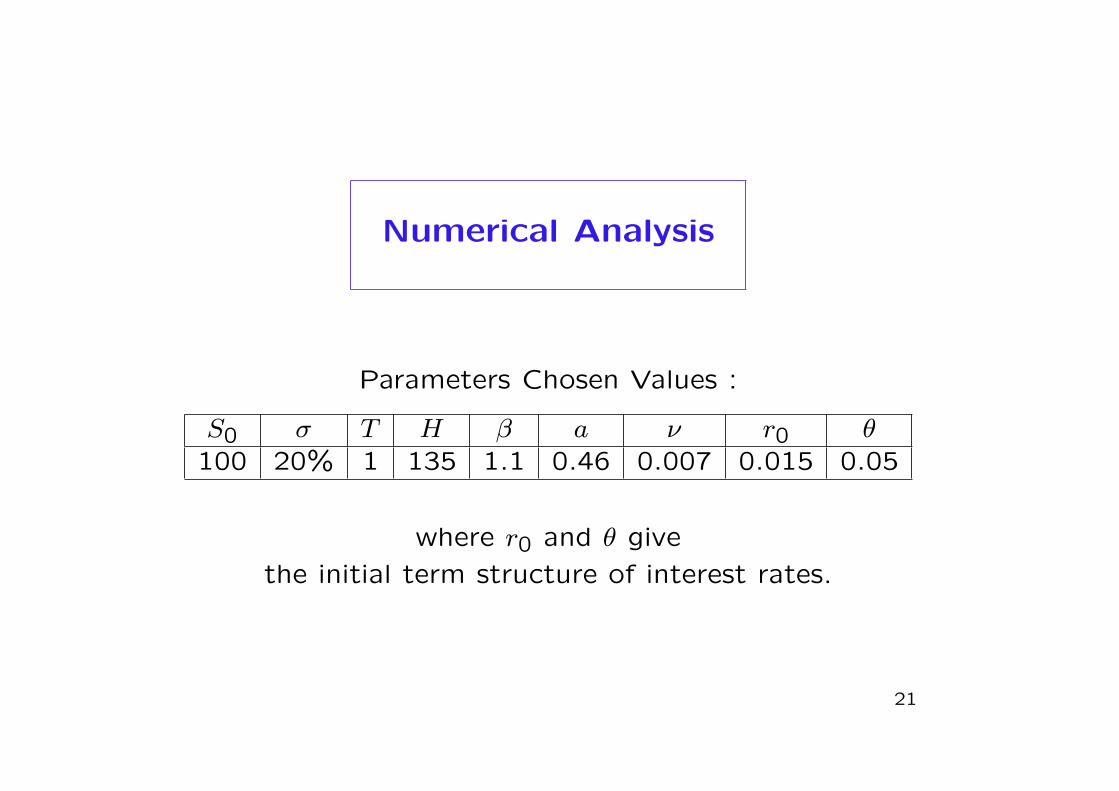
Numerical Analysis

Parameters Chosen Values :

S0 σ T H β a ν r0 θ100 20% 1 135 1.1 0.46 0.007 0.015 0.05

where r0 and θ give

the initial term structure of interest rates.

21

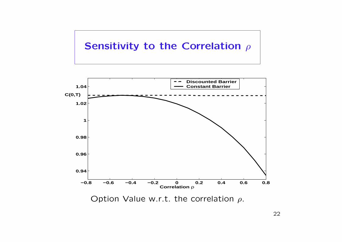
Sensitivity to the Correlation ρ

−0.8 −0.6 −0.4 −0.2 0 0.2 0.4 0.6 0.8

0.94

0.96

0.98

1

1.02

1.04

Correlation ρ

C(0,T)

Discounted BarrierConstant Barrier

Option Value w.r.t. the correlation ρ.

22

Conclusion

The aim is to develop a methodology for the

pricing of barrier options in closed form

and with stochastic interest rates.

When the barrier is constant, quasi-closed-form formulae

can be found thanks to an Extended Fortet Methodology.

When the derivative’s barrier is a discounted one, using time

change techniques we obtain closed-form formulae.

23

Conclusion

-> Beyond the chosen example, our article shows how we

can price barrier options and compute all their Greeks,

under stochastic interest rates.

-> The method yields accurate results (for the prices and

Greeks) much more quickly than Monte-Carlo simulations

24