1

Securitization and Tranching Longevity and

House Price Risk for Reverse Mortgages

Sharon S. Yang1

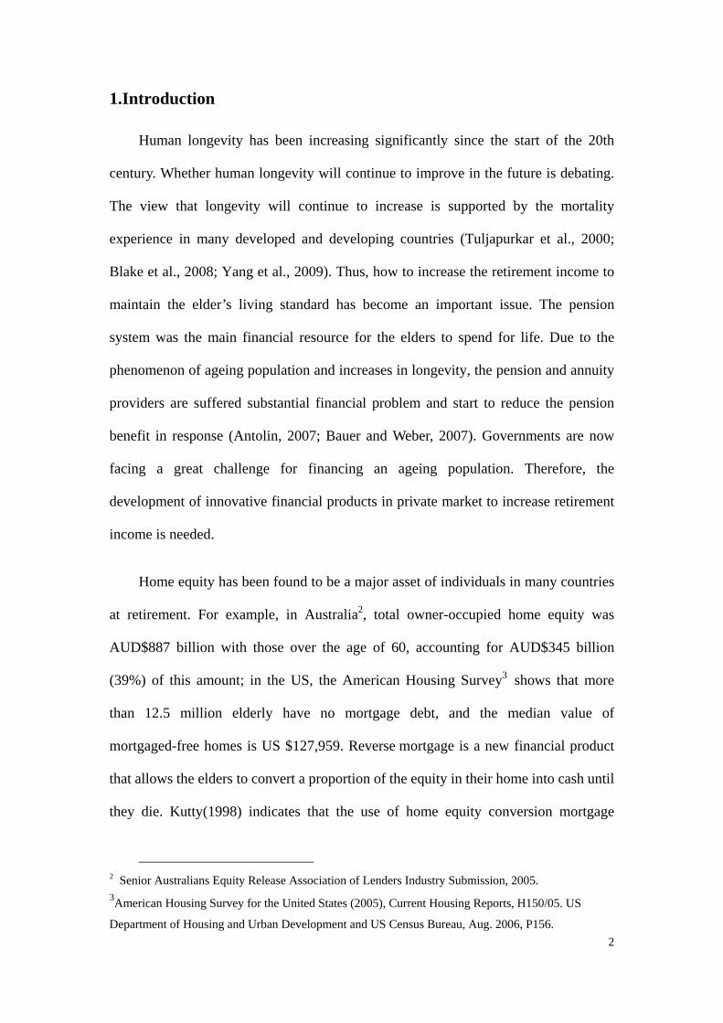
Abstract

Reverse mortgages are new financial products that allow the elders to convert their

home equity into cash until they die. From the provider’s perspective, longevity risk

and house price risk are the major risks involved with reverse mortgages. This paper

proposes a securitization method to transfer the risks associated with reverse

mortgages and focuses on tranching longevity and house price risks for different

investors. The structure of securitization for reverse mortgages is similar to that for

collateralized debt obligation(CDO). Different to price CDO, we model the dynamics

of future mortality and house price instead of default rate. Thus, we model the house

price index using ARMA-GARCH process. To deal with longevity risk for elders, we

use the CBD model (Cairns et al, 2006) to project future mortality. We propose a risk

neutral valuation framework and employ the conditional Esscher transform to price

the fair spreads for different tranche investors. The problems of using static mortality

table and model risk on pricing fair spread are investigated numerically.

Keywords: Reverse mortgage; GARCH Process; Esscher transform

1 Department of Finance, National Central University, Taoyuan, Taiwan. E-mail: syang@ncu.edu.tw.

2

1.Introduction

Human longevity has been increasing significantly since the start of the 20th

century. Whether human longevity will continue to improve in the future is debating.

The view that longevity will continue to increase is supported by the mortality

experience in many developed and developing countries (Tuljapurkar et al., 2000;

Blake et al., 2008; Yang et al., 2009). Thus, how to increase the retirement income to

maintain the elder’s living standard has become an important issue. The pension

system was the main financial resource for the elders to spend for life. Due to the

phenomenon of ageing population and increases in longevity, the pension and annuity

providers are suffered substantial financial problem and start to reduce the pension

benefit in response (Antolin, 2007; Bauer and Weber, 2007). Governments are now

facing a great challenge for financing an ageing population. Therefore, the

development of innovative financial products in private market to increase retirement

income is needed.

Home equity has been found to be a major asset of individuals in many countries

at retirement. For example, in Australia2, total owner-occupied home equity was

AUD$887 billion with those over the age of 60, accounting for AUD$345 billion

(39%) of this amount; in the US, the American Housing Survey3 shows that more

than 12.5 million elderly have no mortgage debt, and the median value of

mortgaged-free homes is US $127,959. Reverse mortgage is a new financial product

that allows the elders to convert a proportion of the equity in their home into cash until

they die. Kutty(1998) indicates that the use of home equity conversion mortgage

2 Senior Australians Equity Release Association of Lenders Industry Submission, 2005. 3American Housing Survey for the United States (2005), Current Housing Reports, H150/05. US

Department of Housing and Urban Development and US Census Bureau, Aug. 2006, P156.

3

products could possibly raise about 29% of the poor elderly homeowners in the U.S.

above the poverty line. In the United States, the department of Housing and Urban

Development (HUD) first introduced the Home Equity Conversion Mortgage (HECM)

program in 1989. In addition to the U.S. market, reverse mortgage products are also

found in the U.K., Australia and in Asian countries of Singapore and Japan.

Reverse mortgages differ from traditional mortgages in the way that the loans

and accrued interests are repaid once when the borrower dies or leave the house.

Unlike traditional mortgage pools, the credit risk in reverse mortgage pools is not

driven by potential default of the loans. The main risk factors are the mortality,

interest rate and the value of the underlying property. If a borrower lives longer than

expected or the decrease in house price, the principal advances and interest accruals

may drive the loan balance above the proceeds of sale the property. Thus, reverse

mortgage is considered to be longevity dependent asset. To develop reverse mortgage

products, risk management has become important for the RM provider to control and

manage the risk. Traditional methods for dealing with the risks associated with

reverse mortgages are using insurance or writing no-negative guarantee. For example,

the HECM program in the United States. The borrower pays a front fee of 2% of the

initial property value as the initial property value. The lenders under this program are

protected against the losses arising when the loan balance exceeds the equity value at

time of settlement. In Britain, most of roll-up mortgages are sold with a

no-negative-equity-guarantee (NNEG) that protects the borrower by capping the

redemption amount of the mortgage at the lesser of the face amount of the loan and

the sale proceeds of the home. The NNEG can be viewed as a European put option on

the mortgaged property. Li et al.(2009) develop a framework for pricing and

managing the risks for the NNEG.

4

Securitization is a new financial innovation to hedge longevity risk. Blake and

Burrows (2001) were the first to advocate the use of mortality-linked securities to

transfer longevity risk to capital markets. The EIB/BNP longevity bond was the first

securitization instrument designed to transfer longevity risk but was not issued finally

and remained theoretical. Survivor swaps, survivor futures and survivor options have

been studied by both academics and practitioners (Blake et al., 2006; Dowd et al.,

2006, Biffis and Blake, 2009; Blake et al. 2010). The first derivative transaction, a

q-forward contract, was issued in January 2008 between Lucida4 and JPMorgan

(Coughlan et al., 2007); the first survivor swap executed in the capital markets

between Canada life and a group of ILS and other investors in July 2008. In this

context, the valuation of mortality-linked securities represents an important research

topic for the development of capital market solutions for longevity risk.

Securitization of longevity risk for annuity business and pension plans have been

widely discussed (Macminn et al., 2006; Michael and Wills, 2007 ). Securitization of

reverse mortgage is still in the early developing stage (Zhai, 2000). Wang et al.(2007)

illustrate a securitization method to hedge the longevity risk inherent in reverse

mortgage products. They study both of survivor bonds and a survivor swap and

demonstrate that securitization can provide an efficient and economical way to hedge

the longevity risk in reverse mortgages. Sherris and Wills(2007) point out that

structuring of longevity risk through a special purpose vehicle requires consideration

of how best to tranche the risk in order to meet different market demands. The

existing literature illustrates the structure and pricing longevity bond for annuity

business(Liao et al. 2007; Wills and Sherris, 2010) not for reverse mortgages. This

article attempts to fill this gap. We further consider the tranche design of longevity

4 A UK-based pension buyout insurer.

5

security for a portfolio of reverse mortgages and illustrate the pricing of fair spreads

for different tranche investors. The structure of the securitization for longevity risk is

similar to the collateralized debt obligation (CDO) for credit risk. Thus, we call it as a

collateralized reverse mortgage obligation (CRMO) in this research. Different to the

survivor swap, the design of CRMO consists on tranching and selling the risk of the

underlying portfolio of reverse mortgages. The lender of reverse mortgages,

investment bank or insurance company, decides to buy protection against the possible

losses due to the longevity risk of the underlying borrower (homeowner). The special

purpose company designs the security with the payoff depending on the uncertainty of

future losses on the underlying reverse mortgage and tranche the risks to different

investors.

To price the fair spread of CRMO for different tranches, we assume a pool of

reverse mortgages. Among the reverse mortgage product in the US market, the home

equity conversion mortgage(HECM) program is considered the most popular one,

which accounts for 95% of the market (Ma and Deng, 2006). Thus, we assume the

pools of loans are under the HECM program. To model the loss for HECM program,

we need to consider both longevity risk and house price risk. The CBD model (Cairns

et al., 2006) is used to capture the dynamic of future mortality for borrowers. To

capture the properties of autocorrelation and volatility clustering that are found in the

literature(Crawford and Fratantoni, 2003; Miller and Peng, 2006; Chen et al., 2010),

we employ ARMA-GARCH process to model the house price dynamic. The risk

neutral pricing framework for the CRMO is derived using conditional Esscher

transform. Since mortality modeling plays an important role in pricing longevity

securities, we also study the impact of mortality modeling on pricing the fair spread

for CRMO. We consider the Lee-carter model(1992) to calculate the result. In

6

addition, the earlier HECM program uses static mortality tables to calculate the loan

value. We also investigate the effect of failing to capture the dynamics of mortality on

securitization of longevity risk for reverse mortgages,

The structure of this paper is organized as follows:

2. Modeling the Risks for HECM Program

2.1 HECM Program

In the US market, HECM program, Fannie Mae's Home Keeper program, and

Financial Freedom's Cash Account Advantage are three major reverse mortgage

programs. HECM Program was authorized by Department of Housing and Urban

Development (HUD) in the Housing and Community Development Act of 1987.

Because the HECM program is insured by the US federal government, it is the most

popular reverse mortgage program and accounts for 95% of the market (Ma and Deng,

2006).

Under the HECM program, the borrower must be at least 62 years age, living in

a single family property that meets HUD’s minimum property standard. The loan can

be taken as four common repayment forms including lump-sum, line of credit, tenure,

and term. The initial loan amount that can be borrowed depends on the initial loan

principal limit (IPL), which is decided according to the borrower’s age, property value

and interest rate.

From the lender’s perspective, the loss occurs when the borrower lives longer

than expected or the decrease in house price, the principal advances and interest

accruals may drive the loan balance above the proceeds of sale the property. To

7

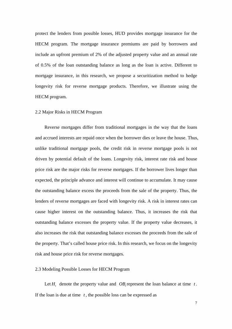
protect the lenders from possible losses, HUD provides mortgage insurance for the

HECM program. The mortgage insurance premiums are paid by borrowers and

include an upfront premium of 2% of the adjusted property value and an annual rate

of 0.5% of the loan outstanding balance as long as the loan is active. Different to

mortgage insurance, in this research, we propose a securitization method to hedge

longevity risk for reverse mortgage products. Therefore, we illustrate using the

HECM program.

2.2 Major Risks in HECM Program

Reverse mortgages differ from traditional mortgages in the way that the loans

and accrued interests are repaid once when the borrower dies or leave the house. Thus,

unlike traditional mortgage pools, the credit risk in reverse mortgage pools is not

driven by potential default of the loans. Longevity risk, interest rate risk and house

price risk are the major risks for reverse mortgages. If the borrower lives longer than

expected, the principle advance and interest will continue to accumulate. It may cause

the outstanding balance excess the proceeds from the sale of the property. Thus, the

lenders of reverse mortgages are faced with longevity risk. A risk in interest rates can

cause higher interest on the outstanding balance. Thus, it increases the risk that

outstanding balance excesses the property value. If the property value decreases, it

also increases the risk that outstanding balance excesses the proceeds from the sale of

the property. That’s called house price risk. In this research, we focus on the longevity

risk and house price risk for reverse mortgages.

2.3 Modeling Possible Losses for HECM Program

Let tH denote the property value and tOB represent the loan balance at time t .

If the loan is due at time t , the possible loss can be expressed as

8

( ) max ,0 , for 1 ~t t tL OB H t xω= − = − (2-1)

where ω is maximal survival age.

We consider the loan is due only when the borrower dies in that year. Thus, the

present value of expected total loss at time 0 is then calculated as

1 11(0) [ ]x rt

t x x t ttTL E e p q Lω− −

− + −== ⋅∑

(2-2)

where 1t xp− denote the survival probability that the borrower aged x and survives to

age x+t-1, 1x tq + − is the probability that the borrower dies in year t.

To transfer the longevity and house price risks for HECM program, we need to

consider both mortality dynamic and house price dynamic, which are described

below.

3. Modeling longevity risk

To examine the effect of longevity risk for reverse mortgages, we need a

stochastic mortality model to capture future mortality dynamics properly. Various

mortality models exist; for example, early developments of stochastic mortality

modeling rely on the age-period effect and pioneering work by Lee and Carter (1992)

and Renshaw and Haberman (2003) offer further analyses of the Lee-Carter model.

Cairns et al. (2006a) instead consider their CBD model of functional relationships,

which deals with mortality rates across ages and thus offers better performance for

older persons. The CBD model also has been adapted to efforts to price longevity

bonds or other mortality-linked securities. In line with the most recent literature on

mortality modeling, we employ CBD stochastic mortality to model longevity risk for

reverse mortgage and calculate the fair spread for the proposed security.

9

3.1 The CBD model

The CBD mortality model we used was proposed in Cairns, Blake, and Down

(2006). They suggest a two-factor model for modeling initial mortality rates instead of

central mortality rate. The mortality rate for a person aged x in year t ( ( , )q t x ) is

modeled as follows:

1 2logit ( , ) ( )t tq t x k k x x= + − (3-1)

where parameter 1tk represents the marginal effect with times on mortality rates and

parameter 2tk portrays the old age effect on mortality rates and x is the mean age.

The future mortality can be projected

3.2 Parameter estimates

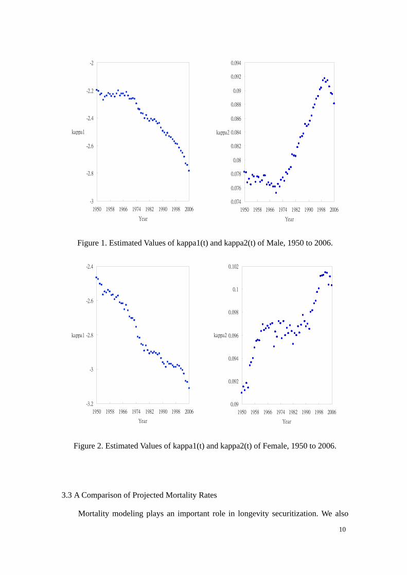
We estimate the parameters in the CBD model by fitting historical U.S. mortality

data from 1950–2006 with the HMD data. The estimated parameters of 1tk and 2

tk

for males and females are depicted in Figure 1 and 2. 1tk shows a down trend and

2tk appear a upward trend. To project future mortality rates, we model 1

tk and 2tk as

follows.

( )

( )

( )

( )

1 1 (1)11

(2)2 22 1

= +t t t

tt t

mu emu e

κ κ

κ κ−

−

⎡ ⎤ ⎡ ⎤ ⎡ ⎤⎡ ⎤+⎢ ⎥ ⎢ ⎥ ⎢ ⎥⎢ ⎥

⎣ ⎦⎢ ⎥ ⎢ ⎥ ⎣ ⎦⎣ ⎦ ⎣ ⎦ (3-2)

10

-3

-2.8

-2.6

-2.4

-2.2

-2

1950 1958 1966 1974 1982 1990 1998 2006

Year

kappa1

0.074

0.076

0.078

0.08

0.082

0.084

0.086

0.088

0.09

0.092

0.094

1950 1958 1966 1974 1982 1990 1998 2006

Year

kappa2

Figure 1. Estimated Values of kappa1(t) and kappa2(t) of Male, 1950 to 2006.

-3.2

-3

-2.8

-2.6

-2.4

1950 1958 1966 1974 1982 1990 1998 2006

Year

kappa1

0.09

0.092

0.094

0.096

0.098

0.1

0.102

1950 1958 1966 1974 1982 1990 1998 2006

Year

kappa2

Figure 2. Estimated Values of kappa1(t) and kappa2(t) of Female, 1950 to 2006.

3.3 A Comparison of Projected Mortality Rates

Mortality modeling plays an important role in longevity securitization. We also

11

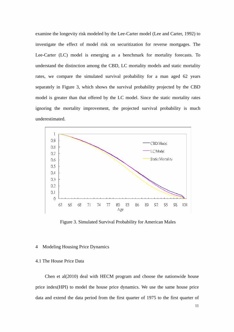
examine the longevity risk modeled by the Lee-Carter model (Lee and Carter, 1992) to

investigate the effect of model risk on securitization for reverse mortgages. The

Lee-Carter (LC) model is emerging as a benchmark for mortality forecasts. To

understand the distinction among the CBD, LC mortality models and static mortality

rates, we compare the simulated survival probability for a man aged 62 years

separately in Figure 3, which shows the survival probability projected by the CBD

model is greater than that offered by the LC model. Since the static mortality rates

ignoring the mortality improvement, the projected survival probability is much

underestimated.

Figure 3. Simulated Survival Probability for American Males

4 Modeling Housing Price Dynamics

4.1 The House Price Data

Chen et al(2010) deal with HECM program and choose the nationwide house

price index(HPI) to model the house price dynamics. We use the same house price

data and extend the data period from the first quarter of 1975 to the first quarter of

12

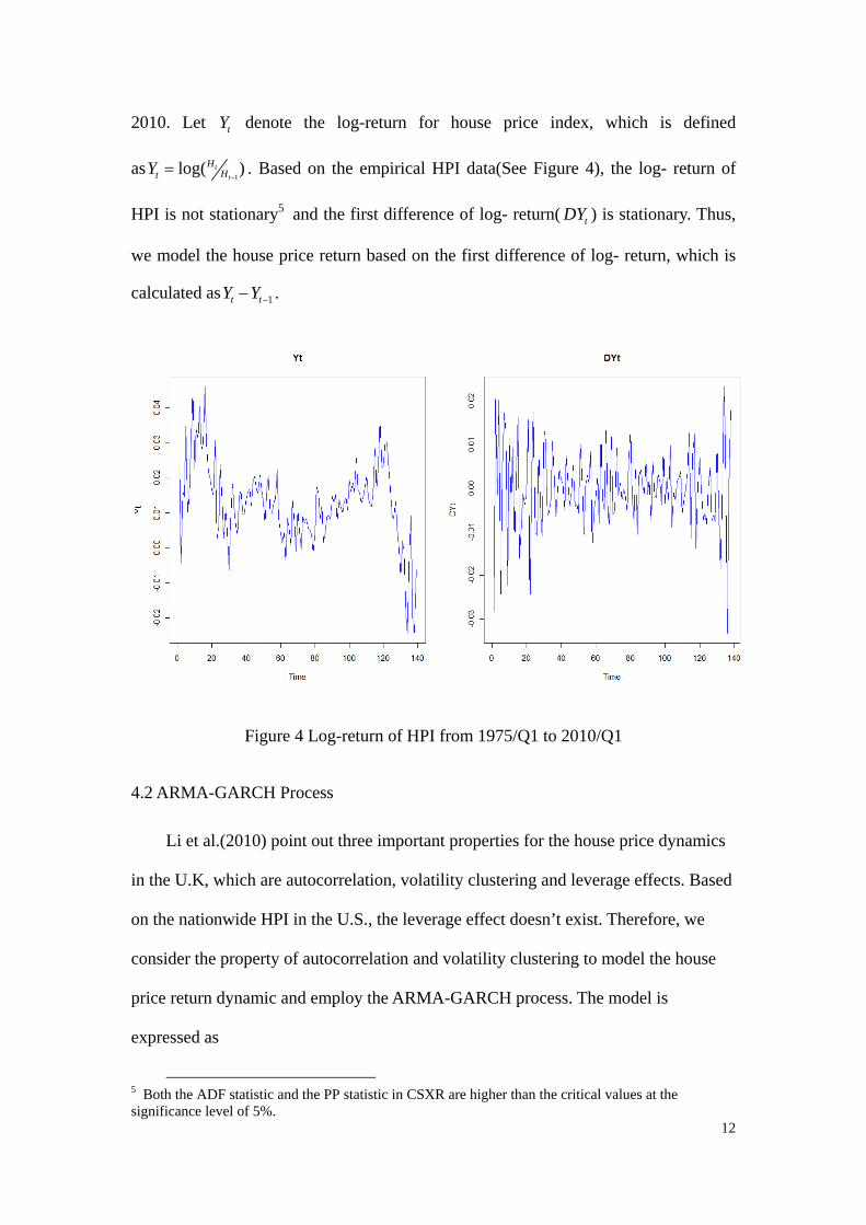
2010. Let tY denote the log-return for house price index, which is defined

as1

log( )tt

HHtY

−= . Based on the empirical HPI data(See Figure 4), the log- return of

HPI is not stationary5 and the first difference of log- return( tDY ) is stationary. Thus,

we model the house price return based on the first difference of log- return, which is

calculated as 1t tY Y −− .

Figure 4 Log-return of HPI from 1975/Q1 to 2010/Q1

4.2 ARMA-GARCH Process

Li et al.(2010) point out three important properties for the house price dynamics

in the U.K, which are autocorrelation, volatility clustering and leverage effects. Based

on the nationwide HPI in the U.S., the leverage effect doesn’t exist. Therefore, we

consider the property of autocorrelation and volatility clustering to model the house

price return dynamic and employ the ARMA-GARCH process. The model is

expressed as

5 Both the ADF statistic and the PP statistic in CSXR are higher than the critical values at the significance level of 5%.

13

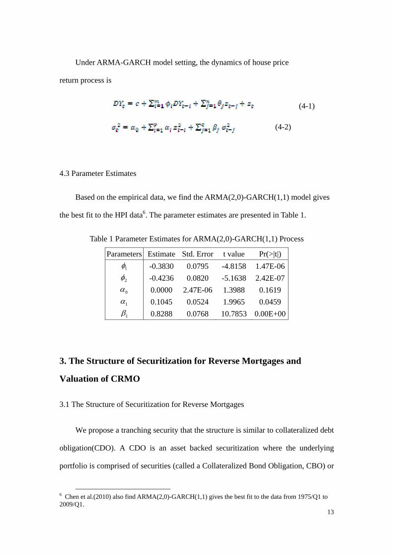
Under ARMA-GARCH model setting, the dynamics of house price

return process is

(4-2)

(4-1)

4.3 Parameter Estimates

Based on the empirical data, we find the ARMA(2,0)-GARCH(1,1) model gives

the best fit to the HPI data6. The parameter estimates are presented in Table 1.

Table 1 Parameter Estimates for ARMA(2,0)-GARCH(1,1) Process

Parameters Estimate Std. Error t value Pr(>|t|)

1φ -0.3830 0.0795 -4.8158 1.47E-06

2φ -0.4236 0.0820 -5.1638 2.42E-07

0α 0.0000 2.47E-06 1.3988 0.1619

1α 0.1045 0.0524 1.9965 0.0459

1β 0.8288 0.0768 10.7853 0.00E+00

3. The Structure of Securitization for Reverse Mortgages and

Valuation of CRMO

3.1 The Structure of Securitization for Reverse Mortgages

We propose a tranching security that the structure is similar to collateralized debt

obligation(CDO). A CDO is an asset backed securitization where the underlying

portfolio is comprised of securities (called a Collateralized Bond Obligation, CBO) or

6 Chen et al.(2010) also find ARMA(2,0)-GARCH(1,1) gives the best fit to the data from 1975/Q1 to 2009/Q1.

14

loans ( called a Collateralized Loan Obligation, CLO) or possibly a mixture of

securities and loans. A CDO consists on tranching and selling the credit risk of the

underlying portfolio. We design a securitization where the underlying portfolio is a

pool of RM products, that is called collateralized reverse mortgage

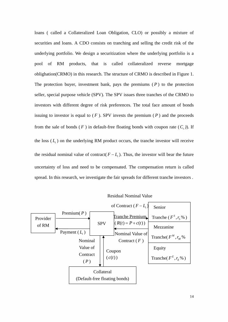
oblighation(CRMO) in this research. The structure of CRMO is described in Figure 1.

The protection buyer, investment bank, pays the premiums ( P ) to the protection

seller, special purpose vehicle (SPV). The SPV issues three tranches of the CRMO to

investors with different degree of risk preferences. The total face amount of bonds

issuing to investor is equal to ( F ). SPV invests the premium ( P ) and the proceeds

from the sale of bonds ( F ) in default-free floating bonds with coupon rate ( tC )). If

the loss ( tL ) on the underlying RM product occurs, the tranche investor will receive

the residual nominal value of contract( tF L− ). Thus, the investor will bear the future

uncertainty of loss and need to be compensated. The compensation return is called

spread. In this research, we investigate the fair spreads for different tranche investors .

SPV

Premium( P )

Payment ( tL )

Senior

Tranche ( , %SSF r )

Mezzanine

Tranche( , %MMF r

Equity

Tranche( , %EEF r )

Collateral (Default-free floating bonds)

Nominal Value of Contract

( P )

Coupon ( ( )c t )

Nominal Value of Contract ( F )

Provider of RM

Residual Nominal Value

of Contract ( tF L− )

Tranche Premium ( ( ) ( )R t P c t= + )

15

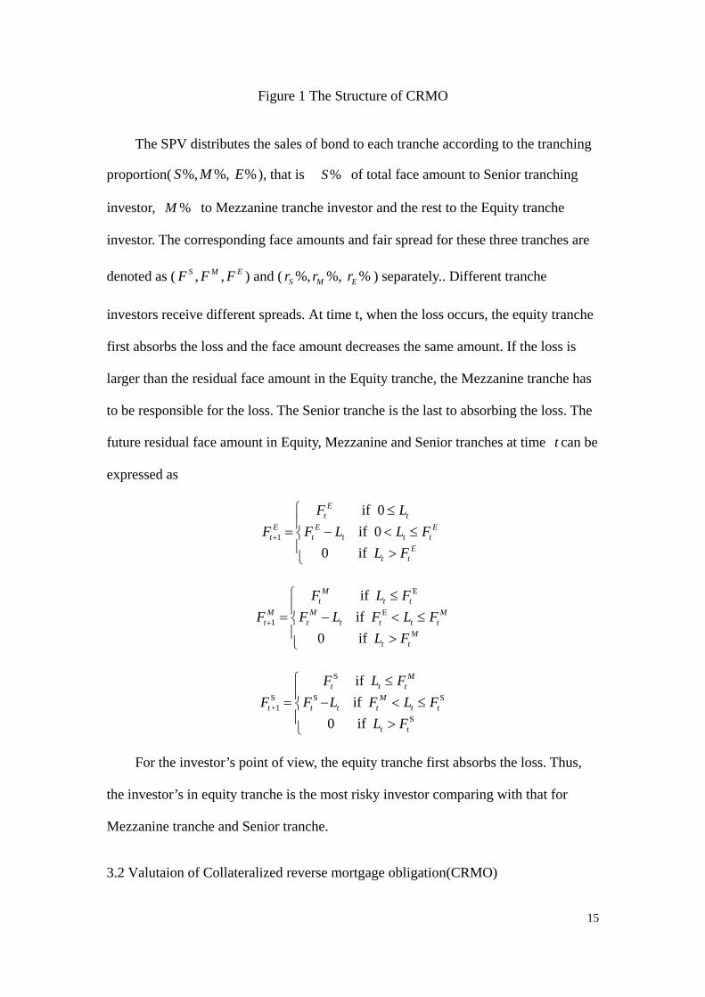
Figure 1 The Structure of CRMO

The SPV distributes the sales of bond to each tranche according to the tranching

proportion( %, %, %S M E ), that is %S of total face amount to Senior tranching

investor, %M to Mezzanine tranche investor and the rest to the Equity tranche

investor. The corresponding face amounts and fair spread for these three tranches are

denoted as ( , ,S M EF F F ) and ( %, %, %S M Er r r ) separately.. Different tranche

investors receive different spreads. At time t, when the loss occurs, the equity tranche

first absorbs the loss and the face amount decreases the same amount. If the loss is

larger than the residual face amount in the Equity tranche, the Mezzanine tranche has

to be responsible for the loss. The Senior tranche is the last to absorbing the loss. The

future residual face amount in Equity, Mezzanine and Senior tranches at time t can be

expressed as

1

if 0 if 0

0 if

Et t

E E Et t t t t

Et t

F LF F L L F

L F+

⎧ ≤⎪= − < ≤⎨⎪ >⎩

E

E1

if if

0 if

Mt t t

M M Mt t t t t t

Mt t

F L FF F L F L F

L F+

⎧ ≤⎪= − < ≤⎨⎪ >⎩

S

S S S+1

S

if if

0 if

Mt t t

Mt t t t t t

t t

F L FF F L F L F

L F

⎧ ≤⎪= − < ≤⎨⎪ >⎩

For the investor’s point of view, the equity tranche first absorbs the loss. Thus,

the investor’s in equity tranche is the most risky investor comparing with that for

Mezzanine tranche and Senior tranche.

3.2 Valutaion of Collateralized reverse mortgage obligation(CRMO)

16

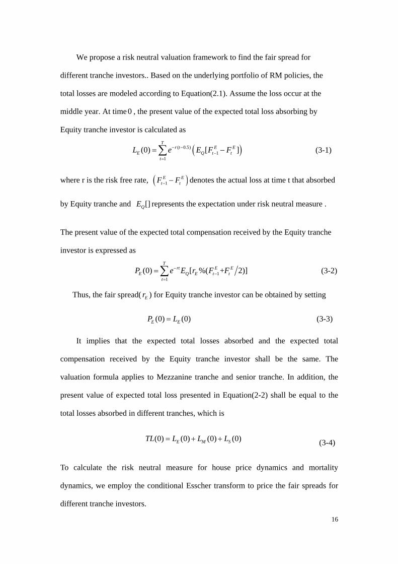
We propose a risk neutral valuation framework to find the fair spread for

different tranche investors.. Based on the underlying portfolio of RM policies, the

total losses are modeled according to Equation(2.1). Assume the loss occur at the

middle year. At time 0 , the present value of the expected total loss absorbing by

Equity tranche investor is calculated as

( )( 0.5)

11

(0) [ ]T

r t E EE Q t t

t

L e E F F− −−

=

= −∑

(3-1)

where r is the risk free rate, ( )1

E Et tF F− − denotes the actual loss at time t that absorbed

by Equity tranche and []QE represents the expectation under risk neutral measure .

The present value of the expected total compensation received by the Equity tranche

investor is expressed as

11

(0) [ %( + 2)]T

rt E EE Q E t t

t

P e E r F F−−

=

=∑

(3-2)

Thus, the fair spread( Er ) for Equity tranche investor can be obtained by setting

(0) (0)E EP L= (3-3)

It implies that the expected total losses absorbed and the expected total

compensation received by the Equity tranche investor shall be the same. The

valuation formula applies to Mezzanine tranche and senior tranche. In addition, the

present value of expected total loss presented in Equation(2-2) shall be equal to the

total losses absorbed in different tranches, which is

(0) (0) (0) (0)E M STL L L L= + + (3-4)

To calculate the risk neutral measure for house price dynamics and mortality

dynamics, we employ the conditional Esscher transform to price the fair spreads for

different tranche investors.

17

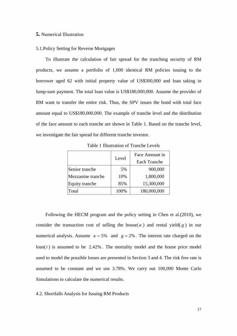
5. Numerical Illustration

5.1.Policy Setting for Reverse Mortgages

To illustrate the calculation of fair spread for the tranching security of RM

products, we assume a portfolio of 1,000 identical RM policies issuing to the

borrower aged 62 with initial property value of US$300,000 and loan taking in

lump-sum payment. The total loan value is US$180,000,000. Assume the provider of

RM want to transfer the entire risk. Thus, the SPV issues the bond with total face

amount equal to US$180,000,000. The example of tranche level and the distribution

of the face amount to each tranche are shown in Table 1. Based on the tranche level,

we investigate the fair spread for different tranche investor.

Table 1 Illustration of Tranche Levels

Level Face Amount in Each Tranche

Senior tranche 5% 900,000 Mezzanine tranche 10% 1,800,000 Equity tranche 85% 15,300,000 Total 100% 180,000,000

Following the HECM program and the policy setting in Chen et al.(2010), we

consider the transaction cost of selling the house(κ ) and rental yield( g ) in our

numerical analysis. Assume 5%κ = and 2%g = . The interest rate charged on the

loan( i ) is assumed to be 2.42% . The mortality model and the house price model

used to model the possible losses are presented in Section 3 and 4. The risk free rate is

assumed to be constant and we use 3.78%. We carry out 100,000 Monte Carlo

Simulations to calculate the numerical results.

4.2. Shortfalls Analysis for Issuing RM Products

18

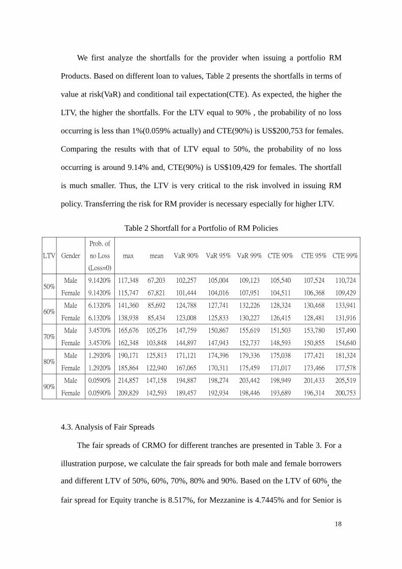
We first analyze the shortfalls for the provider when issuing a portfolio RM

Products. Based on different loan to values, Table 2 presents the shortfalls in terms of

value at risk(VaR) and conditional tail expectation(CTE). As expected, the higher the

LTV, the higher the shortfalls. For the LTV equal to 90% , the probability of no loss

occurring is less than 1%(0.059% actually) and CTE(90%) is US$200,753 for females.

Comparing the results with that of LTV equal to 50%, the probability of no loss

occurring is around 9.14% and, CTE(90%) is US$109,429 for females. The shortfall

is much smaller. Thus, the LTV is very critical to the risk involved in issuing RM

policy. Transferring the risk for RM provider is necessary especially for higher LTV.

Table 2 Shortfall for a Portfolio of RM Policies

LTV Gender

Prob. of

no Loss

(Loss=0)

max mean VaR 90% VaR 95% VaR 99% CTE 90% CTE 95% CTE 99%

50% Male 9.1420% 117,348 67,203 102,257 105,004 109,123 105,540 107,524 110,724

Female 9.1420% 115,747 67,821 101,444 104,016 107,951 104,511 106,368 109,429

60% Male 6.1320% 141,360 85,692 124,788 127,741 132,226 128,324 130,468 133,941

Female 6.1320% 138,938 85,434 123,008 125,833 130,227 126,415 128,481 131,916

70% Male 3.4570% 165,676 105,276 147,759 150,867 155,619 151,503 153,780 157,490

Female 3.4570% 162,348 103,848 144,897 147,943 152,737 148,593 150,855 154,640

80% Male 1.2920% 190,171 125,813 171,121 174,396 179,336 175,038 177,421 181,324

Female 1.2920% 185,864 122,940 167,065 170,311 175,459 171,017 173,466 177,578

90% Male 0.0590% 214,857 147,158 194,887 198,274 203,442 198,949 201,433 205,519

Female 0.0590% 209,829 142,593 189,457 192,934 198,446 193,689 196,314 200,753

4.3. Analysis of Fair Spreads

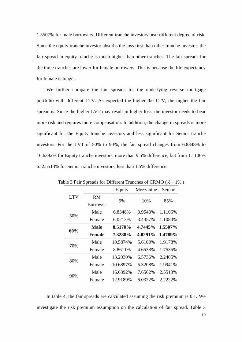
The fair spreads of CRMO for different tranches are presented in Table 3. For a

illustration purpose, we calculate the fair spreads for both male and female borrowers

and different LTV of 50%, 60%, 70%, 80% and 90%. Based on the LTV of 60%, the

fair spread for Equity tranche is 8.517%, for Mezzanine is 4.7445% and for Senior is

19

1.5507% for male borrowers. Different tranche investors bear different degree of risk.

Since the equity tranche investor absorbs the loss first than other tranche investor, the

fair spread in equity tranche is much higher than other tranches. The fair spreads for

the three tranches are lower for female borrowers. This is because the life expectancy

for female is longer.

We further compare the fair spreads for the underlying reverse mortgage

portfolio with different LTV. As expected the higher the LTV, the higher the fair

spread is. Since the higher LVT may result in higher loss, the investor needs to bear

more risk and requires more compensation. In addition, the change in spreads is more

significant for the Equity tranche investors and less significant for Senior tranche

investors. For the LVT of 50% to 90%, the fair spread changes from 6.8348% to

16.6392% for Equity tranche investors, more than 9.5% difference; but from 1.1106%

to 2.5513% for Senior tranche investors, less than 1.5% difference.

Table 3 Fair Spreads for Different Tranches of CRMO ( 1%λ = )

LTV Equity Mezzanine Senior

RM Borrower

5% 10% 85%

50% Male 6.8348% 3.9543% 1.1106%

Female 6.0213% 3.4357% 1.1083%

60% Male 8.5170% 4.7445% 1.5507%

Female 7.3288% 4.0291% 1.4789%

70% Male 10.5874% 5.6100% 1.9178%

Female 8.8611% 4.6538% 1.7535%

80% Male 13.2030% 6.5736% 2.2405%

Female 10.6897% 5.3208% 1.9941%

90% Male 16.6392% 7.6562% 2.5513%

Female 12.9189% 6.0372% 2.2222%

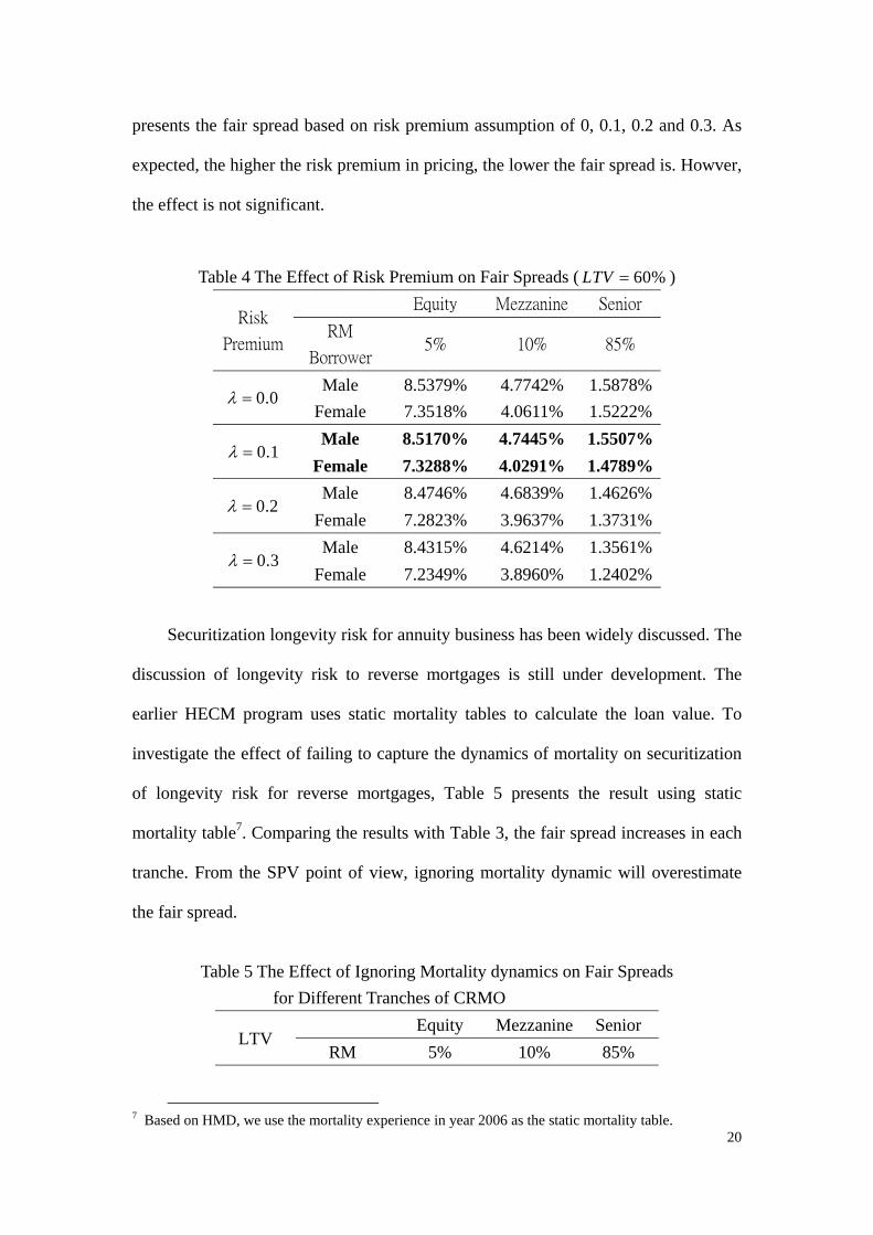
In table 4, the fair spreads are calculated assuming the risk premium is 0.1. We

investigate the risk premium assumption on the calculation of fair spread. Table 3

20

presents the fair spread based on risk premium assumption of 0, 0.1, 0.2 and 0.3. As

expected, the higher the risk premium in pricing, the lower the fair spread is. Howver,

the effect is not significant.

Table 4 The Effect of Risk Premium on Fair Spreads ( 60%LTV = )

Risk

Premium

Equity Mezzanine Senior

RM

Borrower 5% 10% 85%

0.0λ = Male 8.5379% 4.7742% 1.5878%

Female 7.3518% 4.0611% 1.5222%

0.1λ = Male 8.5170% 4.7445% 1.5507%

Female 7.3288% 4.0291% 1.4789%

0.2λ = Male 8.4746% 4.6839% 1.4626%

Female 7.2823% 3.9637% 1.3731%

0.3λ = Male 8.4315% 4.6214% 1.3561%

Female 7.2349% 3.8960% 1.2402%

Securitization longevity risk for annuity business has been widely discussed. The

discussion of longevity risk to reverse mortgages is still under development. The

earlier HECM program uses static mortality tables to calculate the loan value. To

investigate the effect of failing to capture the dynamics of mortality on securitization

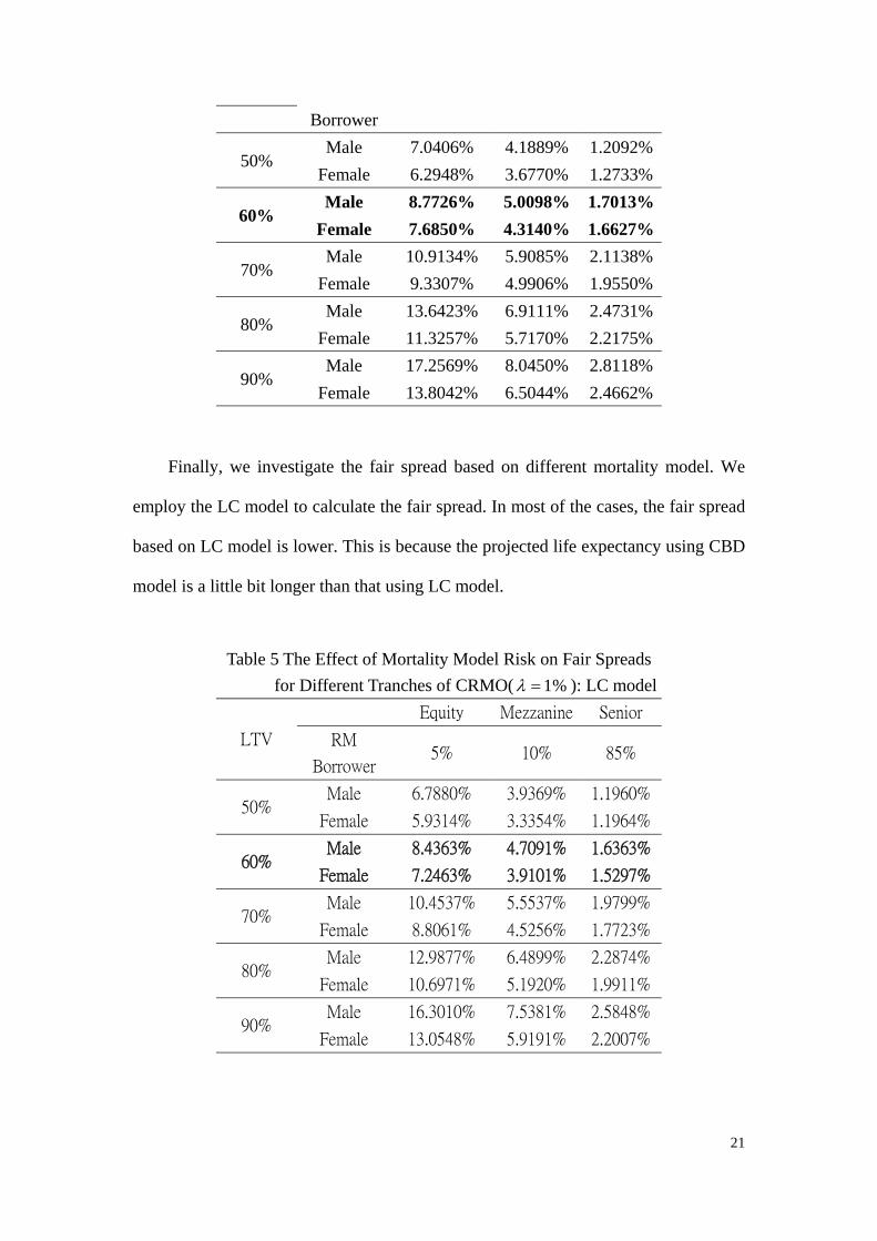
of longevity risk for reverse mortgages, Table 5 presents the result using static

mortality table7. Comparing the results with Table 3, the fair spread increases in each

tranche. From the SPV point of view, ignoring mortality dynamic will overestimate

the fair spread.

Table 5 The Effect of Ignoring Mortality dynamics on Fair Spreads

for Different Tranches of CRMO

LTV Equity Mezzanine Senior

RM 5% 10% 85%

7 Based on HMD, we use the mortality experience in year 2006 as the static mortality table.

21

Borrower

50% Male 7.0406% 4.1889% 1.2092%

Female 6.2948% 3.6770% 1.2733%

60% Male 8.7726% 5.0098% 1.7013%

Female 7.6850% 4.3140% 1.6627%

70% Male 10.9134% 5.9085% 2.1138%

Female 9.3307% 4.9906% 1.9550%

80% Male 13.6423% 6.9111% 2.4731%

Female 11.3257% 5.7170% 2.2175%

90% Male 17.2569% 8.0450% 2.8118%

Female 13.8042% 6.5044% 2.4662%

Finally, we investigate the fair spread based on different mortality model. We

employ the LC model to calculate the fair spread. In most of the cases, the fair spread

based on LC model is lower. This is because the projected life expectancy using CBD

model is a little bit longer than that using LC model.

Table 5 The Effect of Mortality Model Risk on Fair Spreads for Different Tranches of CRMO( 1%λ = ): LC model

LTV

Equity Mezzanine Senior

RM

Borrower 5% 10% 85%

50% Male 6.7880% 3.9369% 1.1960%

Female 5.9314% 3.3354% 1.1964%

60% Male 8.4363% 4.7091% 1.6363%

Female 7.2463% 3.9101% 1.5297%

70% Male 10.4537% 5.5537% 1.9799%

Female 8.8061% 4.5256% 1.7723%

80% Male 12.9877% 6.4899% 2.2874%

Female 10.6971% 5.1920% 1.9911%

90% Male 16.3010% 7.5381% 2.5848%

Female 13.0548% 5.9191% 2.2007%

22

5. Conclusion

In recent years, reverse mortgages are getting more popular in many countries.

To transfer the risk inherent in reverse mortgage products, we propose a securitization

method. The proposed securitization structure differs from existing literature by

introducing the tranche longevity and house price risks for reverse mortgages. The

structure of securitization for reverse mortgages is similar to that for collateralized

debt obligation (CDO). Different to price CDO, we model the dynamics of future

mortality and house price instead of default rate. Thus, we model the house price

index using ARMA-GARCH process. To deal with longevity risk for elders, we use

the CBD model (Cairns et al, 2006) to project future mortality. We propose a risk

neutral valuation framework and employ the conditional Esscher transform to price

the fair spreads for different tranche investors. The problems of using static mortality

table and model risk on pricing fair spread are investigated numerically.

In our numerical analysis, we first analyze the shortfalls for the provider when

issuing a portfolio RM Products. We calculate the fair spreads for both male and

female borrowers and different LTV of 50%, 60%, 70%, 80% and 90%. Since the

equity tranche investor absorbs the loss first than other tranche investor, the fair

spread in equity tranche is much higher than other tranches. The fair spreads for the

three tranches are lower for female borrowers. This is because the life expectancy for

female is longer. We further compare the fair spreads for the underlying reverse

mortgage portfolio with different LTV. As expected the higher the LTV, the higher

the fair spread is. Since the higher LVT may result in higher loss, the investor needs

to bear more risk and requires more compensation. In addition, the change in spreads

is more significant for the Equity tranche investors and less significant for Senior

tranche investors.

23

The earlier HECM program uses static mortality tables to calculate the loan

value. We also investigate the effect of failing to capture the dynamics of mortality on

securitization of longevity risk for reverse mortgages. From the SPV point of view,

ignoring mortality dynamic will overestimate the fair spread. In addition, we employ

the LC model to calculate the fair spread. In most of the cases, the fair spread based

on LC model is lower. This is because the projected life expectancy using CBD model

is a little bit longer than that using LC model. Thus, it implies the use of LC model

will underestimate the fair spread to the investors.

In the light of our analysis in this paper, we also highlight some areas for further

research. First, we do not investigate the issue of jump effect with house price

dynamic and mortality rates. Second, we ignore stochastic interest rate in the

valuation framework. Third, we only consider the reverse mortgages in the form of

lump-sum payment. These three areas would be valuable and interesting extensions

for additional research to tackle.

24

Reference

1. Cairns, Andrew J.G., David Blake and Kevin Dowd (2006). A Two-factor Model

for Stochastic Mortality with Parameter Uncertainty: Theory and Calibration,

Journal of Risk and Insurance, 73: 687-718.

2. Chen, Hua, Samuel H. Cox, Shaun S. Wang(2010).Is the Home Equity

Conversion Mortgage in the United States sustainable? Evidence from pricing

mortgage insurance premiums and non-recourse provisions using the conditional

Esscher transform. Insurance: Mathematics and Economics 46:, 173-185.

3. David Blake, Anja De Waegenaere, Richard MacMinn, Theo Nijman, 2009,

Longevity Risk and Capital Markets: The 2008-2009 Update.

4. Lee, R. D. and L.R. Carter (1992). Modeling and Forecasting U. S. Mortality,

Journal of the American Statistical Association, 87: 659-671.

5. Li, J. S. H., M. R. Hardy and K. S. Tan(2010). On Pricing and Hedging the

No-Negative-Equity Guarantee in Equity Release Mechanisms, Journal of Risk

and Insurance, 77: 449-522.

6. Liao, H.H., S.S. Yang and I.H. Huang(2007). The Design of Securitization for

Longevity Risk: Pricing under Stochastic Mortality Model with Tranche

Technique. Presented at the Third International Longevity Risk and Capital

Market Solutions Symposium, Taipei.

7. Wills, S, and M. Sherris(2010). Securitization, Structuring and Pricing of

Longevity risk, Insurance: Mathematics and Economics, 46 (1), 173-185.

8. Sherris, M. and S. Wills (2007). Financial innovation and the hedging of

longevity risk. Asia Pacific Journal of Risk and Insurance 3(1), 52-64.

9. Zhai, David H.(2000), Reverse Mortgage Securitizations: Understanding and

Gauging the Risks, Special Report, Moody’s Investors Service.