Mortgage Finance and Climate Change:Securitization Dynamics in the Aftermath of

Natural Disasters

Amine Ouazad, HEC Montreal

Matthew E. Kahn, Johns Hopkins University

NYU Stern Climate Finance, Dec 4, 2020

Big Questions: Climate Risk in Financial Markets

I Who bears climate risk?I Houses mostly purchased using mortgage credit. Mortgages

are traded, securitized.I Risk sharing between borrowers and: commercial banks,

non-bank lenders, Government Sponsored Enterprises (GSEs),Private Label Securitizers.

I Questions of optimal risk-sharing

I Who is more informed?I Asymmetric observability of current local climate risk.I Ambiguity of future climate risk probability distributions.

I Is climate risk priced in?

I Who adapts to climate risk?I Political economy of climate risk sharing.I Large amount of policy intervention in the mortgage market.I Design of institutions to make the economy resilient?

A Securitization Chain

BorrowerInterest Rate−−−−−−−→ Lender

Guarantee Fee−−−−−−−−→ Securitizer

I A `Market for Lemons' in local natural disaster risk?

I Observing such selection at the conforming loan limit:I Government Sponsored Enterprises, Fannie and Freddie use

FHFA-set observable rules for purchasing mortgages andpricing securitization.

I Sharp discontinuity in lenders' ability to securitize theiroriginated mortgages at the conforming limit.

I Natural experiment: Conforming limits varying across

counties and across time `biting' at di�erent arbitrary points.

Questions:

1. Do local natural disasters lead to more origination and

securitization of conforming loans?

2. Are conforming loans better or worse risk?

3. How can the GSEs adapt?

Findings

1. Do local natural disasters lead to more securitization of

conforming loans relative to jumbo loans?

↑ in volume and securitization of conforming loans relative to jumbo

loans.

Increasing adverse selection after disaster.

Impact increases for 3 years after the event.Greater increase in securitization & bunching with disaster �new news�.

2. Are conforming loans better or worse risk?Higher rates of delinquency and default.

3. How can the GSEs adapt? An asymmetric information

structural model for counterfactuals.

→ adjust guarantee fees and securitization standards.

Billion Dollar Events

Source: Estimates from Weinkle et al (2018).

Climate data: Hurricanes, Elevation, Wetland

1. High Resolution Storm Surge Predictions: NOAA's

hurricane model: Sea, Lake, and Overland Surges from

Hurricanes (SLOSH).

2. HUD Inspections of housing units.

3. NOAA's Atlantic Hurricane Data Set �HURDAT2�1851-2018.

3.1 Geocoded Hurricane path with wind speed and time-varyingradius.

3.2 64kt wind radius: Sa�r Simpson Scale.

4. USGS's Elevation data: Shuttle Radar TopographyMission.

4.1 Satellite measurements of elevation by 30m x 30m cell.

5. USGS's National Land Cover data base.

5.1 Open water, Woody wetlands, Emergent wetlands.

Treatment Area Geography: the Example of Sandy

Financial data: Three Key Data Sources

1. McDash data set from Black Knight Financial.I Data from servicers, covers about 65% of the market, since

1989.I FICO scores, monthly payment history, loan amortization

structure (interest rate; IO, fully amortizing, balloon payment;ARM, FRM).

I First and second mortgage: combined LTVI 5-digit ZIP code data.

2. The FFIEC's Home Mortgage Disclosure Act data setI Larger coverage, more granular (census tract), but no payment

history.I Matched to lenders' balance sheets (Transmittal Sheets).

3. Banks' Balance SheetsI Quarterly Reports of Income and Condition (Bank-Level) →

balance sheet liquidity, regulator, bank type.

Baseline Discontinuities:Applications and Credit Score

I Home Mortgage Disclosure Act data.

Baseline Discontinuities:Securitization Rates, Lender Liquidity

I Home Mortgage Disclosure. Reports of Income and Condition.

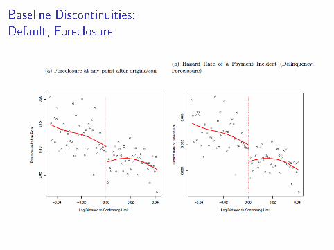
Baseline Discontinuities:Default, Foreclosure

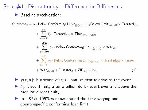
Spec #1: Discontinuity � Di�erence-in-Di�erences

I Baseline speci�cation:

Outcomeit = α · BelowConforming Limitijy(t,d) + γBelowLimitijy(t,d) × Treatedj(i)

++T∑

t=−T

ξt · Treatedj(i) × Timet=y−y0(d)

+2016∑

y=1995

ζy · BelowConforming Limitijy(t,d) × Yeary(t)

++T∑

t=−T

δt · BelowConforming Limitijy(t,d) × Treatedj(i) × Timet

+ Yeary(t,d) + Disasterd + ZIPj(i) + εit , (1)

I y(t, d): hurricane year; i : loan, t: year relative to the event.

I δt : discontinuity after a billion dollar event over and above the

baseline discontinuity.

I In a 95%�105% window around the time-varying and

county-speci�c conforming loan limit.

Two Sources of Identifying Variation

I Idiosyncratic extent of hurricane impacts conditional on the

satured set of local f.e.s

NOAA's Seasonal outlook [...] predicts the number ofnamed tropical storms, hurricanes, and major hurricanes[...] But that's where the reliable long-range sci-

ence stops. The ability to forecast the location and

strength of a landfalling hurricane is based on a va-

riety of factors, details that present themselves days,

not months, ahead of the storm.

I Conforming loan limits and guarantee fees are set nationally

every year.

The Federal Housing Finance Agency (FHFA) publishes an-nual conforming loan limits that apply to all conventionalmortgages delivered to Fannie Mae.

Spec #2: Bunching � Di�erence-in-Di�erences

#Below Limitjt −#Above Limitjt#Below Limitjt + #Above Limitjt

= γvTreatedj ++T∑

t=−T

ξvt · Treatedj × Timet

+ Yearvolumey(t,d) + Disastervolume

d + ZIPvolumej + εvjt , (2)

I #Below Limitjt (#Above Limitjt): number of mortgages with

loan amounts in the 10% segment below (above) the

conforming limit.I Coe�cients of interest are the ξvt , t ≥ 0, the impact of the

natural of the disaster for each postdisaster year

t = y − y0(d). t = −5, . . . ,+4.I Coe�cients ξvt , t < 0: pre-trends in the discontinuity prior to

the disaster.I Coe�cient γv : the average di�erence in the size of the

discontinuity between the treated and untreated zip codes.

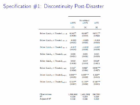
Speci�cation #1: Discontinuity Post-Disaster

Speci�cation #1: Adverse Selection

Speci�cation #1: Adverse Selection

Speci�cation #2: Bunching Post Disaster

Counterfactual Approach: Simulating an Increase in DisasterRisk without the GSEs' Securitization Activity

I Estimating counterfactuals requires a model.

I Second-degree price discrimination: lenders o�er a menu ofchoices.I Households self-select based on their default driver ε.I → reproduce the observed discontinuity.

I Simulate the impact of an increase in disaster risk π on

the equilibrium of the mortgage market.

I Disaster risk ↑ lead to little change in origination volumes in

the conforming segment when the GSEs securitize, yet very

large sensitivity to �ood risk when we withdraw the GSE

securitization option.

Introducing Disaster Risk (1%)

New equilibrium in red.

Counterfactual Simulation. Shutting down GSEsecuritization

Response of approval rates to the introduction of a 1% disaster risk.

New equilibrium in orange.

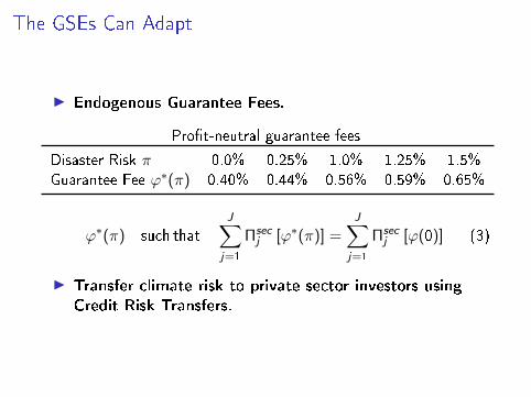
The GSEs Can Adapt

I Endogenous Guarantee Fees.

Pro�t-neutral guarantee fees

Disaster Risk π 0.0% 0.25% 1.0% 1.25% 1.5%

Guarantee Fee ϕ∗(π) 0.40% 0.44% 0.56% 0.59% 0.65%

ϕ∗(π) such that

J∑j=1

Πsecj [ϕ∗(π)] =

J∑j=1

Πsecj [ϕ(0)] (3)

I Transfer climate risk to private sector investors using

Credit Risk Transfers.

A Research Agenda

Questions:

I Can �nancial products diversify climate risk?I Does the packaging of climate-exposed assets reduce risk or

rather lead to Fault Lines that endanger the stability of themortgage market?

I Do private counterparties adapt to the rising default risk?I by charging higher fees, pricing in the risk of climate shocks?

I Is climate a Weitzman type tail risk or rather part ofconventional volatility?I A �climate� equity premium puzzle?

I How do agents behave in the face of ambiguous risk?

→ Exploring each part of a general equilibrium asset pricing model.

→ Does climate risk a�ect the fundamental theorems of asset

pricing?