Embed Size (px)
Citation preview

PRICING AND DYNAMIC HEDGING OF SEGREGATED
FUND GUARANTEES
by
Qipin He
B.Econ., Nankai University, 2006
a Project submitted in partial fulfillment
of the requirements for the degree of
Master of Science
in the Department
of
Statistics and Actuarial Science
c© Qipin He 2010
SIMON FRASER UNIVERSITY
Fall 2010
All rights reserved. However, in accordance with the Copyright Act of Canada,
this work may be reproduced, without authorization, under the conditions for
Fair Dealing. Therefore, limited reproduction of this work for the purposes of
private study, research, criticism, review and news reporting is likely to be
in accordance with the law, particularly if cited appropriately.

APPROVAL
Name: Qipin He
Degree: Master of Science
Title of Project: Pricing and Dynamic Hedging of Segregated Fund Guarantees
Examining Committee: Dr. Derek Bingham
Chair
Dr. Cary Chi-Liang Tsai
Senior Supervisor
Simon Fraser University
Dr. Gary Parker
Supervisor
Simon Fraser University
Dr. Yi Lu
External Examiner
Simon Fraser University
Date Approved:
ii

Abstract
Guaranteed minimum maturity benefit and guaranteed minimum death benefit offered by
a single premium segregated fund contract are priced. A dynamic hedging approach is used
to determine the value of these guarantees. Cash flow projections are used to analyze the
loss or profit to the insurance company. Optimally exercised reset options are priced by the
Crank-Nicolson method. Reset options, assuming they are exercised only when the funds
exceed a given threshold, are priced using simulations. Finally, we study the distribution of
the loss or profit for segregated funds with reset option under a dynamic hedging strategy
with an allowance for transaction costs.
Keywords: Guaranteed Minimum Maturity Benefit, Guaranteed Minimum Death Benefit,
Charge Rate, Black-Scholes European Put Option, Dynamic Hedging, Hedge Error, Trans-
action Cost, Transaction Costs Adjusted Hedge Volatility, Reset Option, Crank-Nicolson
iii

Acknowledgments
I would like to thank my supervisor Dr. Cary Chi-Liang Tsai, who chose such an interesting
thesis topic for me and helped me conquer many technical problems. Working with him, I
have learnt a lot about actuarial science. I would also like to give my special thanks to Dr.
Gary Parker for his guidance during the last a few months of my project writing. Every time
talking with him, I was always inspired by his intuitive ideas and suggestions. In addition,
I would like to thank Dr. Yi Lu for her time and patience spent on my project.
At last, I want to give my gratitude to all of my friends at Simon Fraser University.
With them, I had a fun and productive two-year time of my graduate study.
iv

Contents
Approval ii
Abstract iii
Acknowledgments iv
Contents v
List of Tables vii
List of Figures viii
1 Introduction 1
2 The model 4
2.1 The model for the asset . . . . . . . . . . . . . . . . . . . . . . . . . . . . . . 4
2.2 Pricing the segregated fund guarantees . . . . . . . . . . . . . . . . . . . . . . 6
3 Dynamic hedging approach 9
3.1 Discrete time hedging strategy . . . . . . . . . . . . . . . . . . . . . . . . . . 9
3.2 Transaction costs adjusted hedge volatility . . . . . . . . . . . . . . . . . . . . 11
3.3 Hedging for the segregated fund contract . . . . . . . . . . . . . . . . . . . . . 15
3.3.1 The initial hedge cost . . . . . . . . . . . . . . . . . . . . . . . . . . . 15
3.3.2 Re-balancing the hedging portfolio . . . . . . . . . . . . . . . . . . . . 19
3.4 The cash flows . . . . . . . . . . . . . . . . . . . . . . . . . . . . . . . . . . . 26
v

4 Valuation of the reset option 38
4.1 Introduction of Crank-Nicolson method . . . . . . . . . . . . . . . . . . . . . 38
4.1.1 Discretization techniques . . . . . . . . . . . . . . . . . . . . . . . . . 38
4.1.2 Solving the PDE . . . . . . . . . . . . . . . . . . . . . . . . . . . . . . 40
4.2 Pricing the segregated fund with reset option . . . . . . . . . . . . . . . . . . 42
4.2.1 Optimality statement . . . . . . . . . . . . . . . . . . . . . . . . . . . 42
4.2.2 Boundary values . . . . . . . . . . . . . . . . . . . . . . . . . . . . . . 43
4.2.3 Implementation . . . . . . . . . . . . . . . . . . . . . . . . . . . . . . . 43
4.2.4 The solution of the charge rate . . . . . . . . . . . . . . . . . . . . . . 45
4.2.5 Further analysis of the charge rate . . . . . . . . . . . . . . . . . . . . 47
4.3 Hedging the segregated fund with reset option . . . . . . . . . . . . . . . . . . 54
5 Conclusion 57
A Some proofs 59
A.1 The proof of Equation (3.3) . . . . . . . . . . . . . . . . . . . . . . . . . . . . 60
A.2 The proof of Equation (3.4) . . . . . . . . . . . . . . . . . . . . . . . . . . . . 61
Bibliography 63
vi

List of Tables
3.1 The hedge costs with σ . . . . . . . . . . . . . . . . . . . . . . . . . . . . . . 13
3.2 The hedge costs with σ . . . . . . . . . . . . . . . . . . . . . . . . . . . . . . 13
3.3 The hedge errors net of the transaction costs with σ. The annual charge is
deducted . . . . . . . . . . . . . . . . . . . . . . . . . . . . . . . . . . . . . . . 13
3.4 The hedge errors net of the transaction costs with σ. The annual charge is
deducted . . . . . . . . . . . . . . . . . . . . . . . . . . . . . . . . . . . . . . . 14
3.5 The cash flows in the mid-years . . . . . . . . . . . . . . . . . . . . . . . . . . 27
4.1 Solving for European put options with 1000 time grids . . . . . . . . . . . . . 41
4.2 Instantaneous charge rates of Type I contracts . . . . . . . . . . . . . . . . . 45
4.3 Instantaneous charge rates of Type II contracts . . . . . . . . . . . . . . . . . 45
4.4 The sample mean and standard deviation of the fund value and GMMB payoff
at maturity . . . . . . . . . . . . . . . . . . . . . . . . . . . . . . . . . . . . . 49
4.5 The sample mean and standard deviation of the duration and maturity guar-
antee . . . . . . . . . . . . . . . . . . . . . . . . . . . . . . . . . . . . . . . . . 50
4.6 The sample mean and standard deviation of the total payment and yield at
maturity . . . . . . . . . . . . . . . . . . . . . . . . . . . . . . . . . . . . . . . 51
4.7 The sample mean and standard deviation of the NPV of the cash flows . . . . 53
4.8 The mean and standard deviation of the NPV of the cash flows . . . . . . . . 54
4.9 The mean and standard deviation of the NPV of the cash flows with and
without hedging . . . . . . . . . . . . . . . . . . . . . . . . . . . . . . . . . . 55
vii

List of Figures
2.1 Examples of asset price processes . . . . . . . . . . . . . . . . . . . . . . . . . 5
2.2 The instantaneous charge rates . . . . . . . . . . . . . . . . . . . . . . . . . . 5
2.3 The composition of the instantaneous charge rates . . . . . . . . . . . . . . . 6
3.1 The hedge errors net of the transaction costs at each hedge time . . . . . . . 14
3.2 The initial hedge costs for the annually hedging strategy . . . . . . . . . . . . 16
3.3 The initial hedge costs for the monthly hedging strategy . . . . . . . . . . . . 17
3.4 The initial hedge costs for the weekly hedging strategy . . . . . . . . . . . . . 18
3.5 Type I, Age 30, $100 single premium . . . . . . . . . . . . . . . . . . . . . . . 20
3.6 Type I, Age 60, $100 single premium . . . . . . . . . . . . . . . . . . . . . . . 21
3.7 Type I, Age 80, $100 single premium . . . . . . . . . . . . . . . . . . . . . . . 22
3.8 Type II, Age 30, $100 single premium . . . . . . . . . . . . . . . . . . . . . . 23
3.9 Type II, Age 60, $100 single premium . . . . . . . . . . . . . . . . . . . . . . 24
3.10 Type II, Age 80, $100 single premium . . . . . . . . . . . . . . . . . . . . . . 25
3.11 Net Cash flows of Type I contract, Age 30 . . . . . . . . . . . . . . . . . . . . 29
3.12 Net Cash flows of Type I contract, Age 60 . . . . . . . . . . . . . . . . . . . . 30
3.13 Net Cash flows of Type I contract, Age 80 . . . . . . . . . . . . . . . . . . . . 31
3.14 Net Cash flows of Type II contract, Age 30 . . . . . . . . . . . . . . . . . . . 32
3.15 Net Cash flows of Type II contract, Age 60 . . . . . . . . . . . . . . . . . . . 33
3.16 Net Cash flows of Type II contract, Age 80 . . . . . . . . . . . . . . . . . . . 34
3.17 The mean and standard deviation of the NPV of the cash flows. Type I, Age
30 and $100 single premium contract is used . . . . . . . . . . . . . . . . . . . 36
3.18 Comparison of the distributions of the NPV of the cash flows . . . . . . . . . 37
3.19 Comparison of the percentiles of the NPV of the cash flows . . . . . . . . . . 37
viii

4.1 Discretization of the Black-Scholes pde . . . . . . . . . . . . . . . . . . . . . . 41
4.2 The solution of instantaneous charge rate . . . . . . . . . . . . . . . . . . . . 46
4.3 The simulated density distributions of the fund value and GMMB payoff at
maturity . . . . . . . . . . . . . . . . . . . . . . . . . . . . . . . . . . . . . . . 49
4.4 The simulated density distributions of the duration and maturity guarantee . 50
4.5 The simulated density distributions of the total payment and yield at maturity 52
4.6 The simulated density distributions of the NPV of the cash flows . . . . . . . 53
4.7 The density distributions and percentiles of the NPV of the cash flows . . . . 55
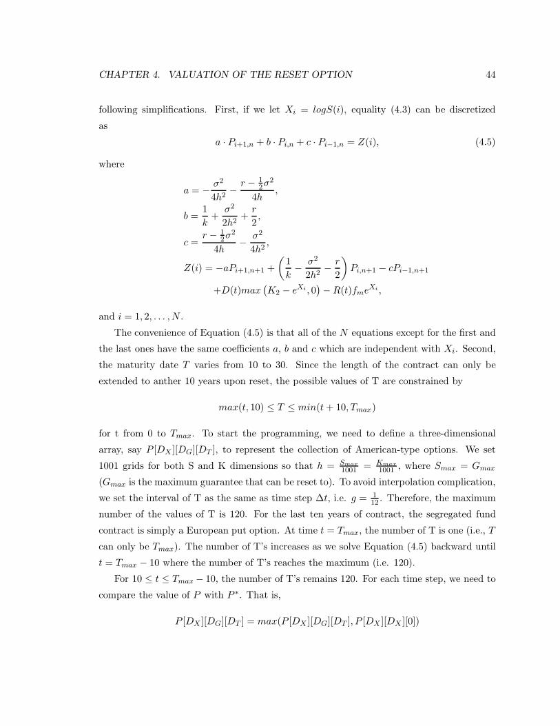
4.8 The density distributions and percentiles of the NPV of the cash flows with
and without hedging . . . . . . . . . . . . . . . . . . . . . . . . . . . . . . . . 56
ix

Chapter 1
Introduction
A segregated fund is a type of equity-linked insurance contract commonly sold in Canada.
Policyholders are usually offered a broad selection of investment choices and these funds are
fully separated from the company’s general investment funds (Wikipedia, http://en.wikiped-
ia.org/wiki/Segregated fund). The segregated fund normally provides a guaranteed mini-
mum maturity benefit (GMMB) and a guaranteed minimum death benefit (GMDB). The
benefit guarantee is 75% or higher percentage of the initial fund value (Moodys Looks At
Guaranteed Segregated Funds In Canada & Their Risks, August 2001). In case of death
within the term of the contract or at maturity, the benefit amount is the maximum of the
accumulated fund value and the guarantee.
Segregated fund guarantees are financial guarantees. In most cases the payoffs of the
benefits are zero, while due to some poor investment a considerable amount of additional
money is needed to compensate the gap between the fund value and the guarantee level.
The risk arisen by the highly skewed payoff distribution cannot be diversified by pooling
segregated fund contracts with the same maturity date.
One approach commonly used in practice is called dynamic hedging which considers the
segregated fund as a special type of European put option (Great-West Life Segregated Fund
Policies Information Folder, May 2010). Many issues of this approach have been discussed
in mathematical finance such as Leland (1985) and Toft (1996), and was applied to the
segregated fund by Boyle and Hardy (1997) and Hardy (2000, 2001, 2002). A hedging
portfolio consisting of some risk-free bond and risky asset is held at the beginning of the
contract term and the segregated fund is several times before it matures. Leland (1985)
introduced the transaction costs adjusted hedge volatility (Leland ’s volatility) with which
1
CHAPTER 1. INTRODUCTION 2
the hedge errors net of transaction costs tends to zero as the hedge interval decreases. Toft
(1996) derived expressions for the mean and variance of the hedge error and transaction cost.
In Boyle and Hardy (1997) and Hardy (2000, 2002) dynamic hedging was used to hedge
a segregated fund contract. The results derived were based on simulation and Leland ’s
volatility was not adopted.
Segregated fund contract lasts for at least 10 years (Moodys Looks At Guaranteed Seg-
regated Funds In Canada & Their Risks, August 2001). Within the contract term, policy-
holders are given the option to reset the contract several times within some period (usually
one or two times per year). Upon reset, the GMMB and GMDB would be reset to the
guarantee levels of the current fund value, and the contract lasts for another 10 years from
the time of reset. This feature adds more complexity to the valuation of the segregated fund.
In Armstrong (2001) some techniques for the optimal reset decisions to a simplified segre-
gated fund contract were discussed. Windcliff, Forsyth and Vetzal (2001a, 2001b and 2002)
discussed the valuation of segregated funds with reset options by employing finite difference
methods; one of which, commonly used by financial engineers, is call the Crank-Nicolson
method. This method requires some discretization techniques and optimality assumptions
to approximately solve a collection of partial differential equations (PDE) backwards for the
price of the contract. The uncertainties of the contract duration and the guarantee benefits
add more volatility to the risks of the segregated fund.
The main focus of this project is to discuss some risk issues arisen by the features of
the segregated fund and apply dynamic hedging approach to both no-reset-allowed (stan-
dard) and reset-allowed (extendable) segregated fund contracts. For simplicity, no lapse is
assumed. Two types of the segregated fund contracts are considered. Type I offers 100%
GMMB level and 75% GMDB level and Type II offers 75% GMMB level and 100% GMDB
level. We use the traditional geometric Brownian motion to model the risky asset value
that the premium of the segregated fund is invested into. We also assume that the capital
set by dynamic hedging approach is put into a zero-coupon bond which offers a constant
risk-free interest rate. Note that all the analysis in this project do not consider either model
risk or parameter risk. In different time period or other situations, the model employed and
the parameters estimated in this project might not be accurate. The idea is to provide a
convenient way to focus on the main purpose of this project.
The remainder of the project is organized as follows: in Chapter 2, the model is intro-
duced and the standard segregated fund is priced. Chapter 3 discusses dynamic hedging

CHAPTER 1. INTRODUCTION 3
approach and the corresponding cash flows. In the following chapter, the reset option is
priced and discussed, and the distribution of the loss or profit for segregated funds with
reset option under a dynamic hedging strategy is studied.

Chapter 2
The model
2.1 The model for the asset
We assume that the market price of the asset in which the segregated fund is invested follows
a geometric Brownian motion. That is, if St is the asset price at time t, then
dSt = µStdt + σStdBt, (2.1)
where µ is the drift rate, σ is the volatility and Bt stands for a standard Brownian motion.
This implies that the return on asset over discrete time intervals follows an independent
normal distribution. That is,
logSt2
St1
∼ N
((µ − 1
2σ2)(t2 − t1), σ
2(t2 − t1)
),
where t2 > t1 ≥ 0 and N(a, b) stands for a normal distribution with mean a and variance b.
We also assume that the fund premium is invested in S&P/TSX Composite Index (the
name was TSE 300 before May 1, 2002). Based on the monthly data from 2000 to 2009 (Data
source: Yahoo! Finance, http://finance.yahoo.com), the estimated values of the parameters
in Equation (2.1) are µ = 0.04 and σ = 0.16.
Figure 2.1 shows four types of asset price sample paths for 10 years based on the esti-
mated parameters. The dashed and dotted parallel lines represent the 100% and 75% levels
of the initial asset value. Figure 2.1 (a) and (b) give two opposite price path trends, while
Figure 2.1 (c) and (d) show the price paths that fluctuate around the 100% guarantee level,
the difference being that (c) ends up at the safe zone (above both parallel lines) and (d) is
subject to the 100% guarantee risk.
4

CHAPTER 2. THE MODEL 5
0 2 4 6 8 10
0.51.0
1.52.0
2.5(a)
Time
Stoc
k pric
e
0 2 4 6 8 10
0.51.0
1.52.0
2.5
(b)
Time
Stoc
k pric
e
0 2 4 6 8 10
0.51.0
1.52.0
2.5
(c)
Time
Stoc
k pric
e
0 2 4 6 8 10
0.51.0
1.52.0
2.5
(d)
Time
Stoc
k pric
e
Figure 2.1: Examples of asset price processes
0 20 40 60 80
0.000
0.005
0.010
0.015
0.020
0.025
0.030
0.035
Under actuarial method
Age
Charg
e rate
Type I
Type II
0 20 40 60 80
0.000
0.005
0.010
0.015
0.020
0.025
0.030
0.035
Under risk−neutral method
Age
Charg
e rate
Type I
Type II
Figure 2.2: The instantaneous charge rates

CHAPTER 2. THE MODEL 6
0 20 40 60 80
0.000
0.010
0.020
0.030
Type I under actuarial methodAge
Charg
e rate
0 20 40 60 80
0.000
0.010
0.020
0.030
Type II under actuarial methodAge
Charg
e rate
0 20 40 60 80
0.000
0.010
0.020
0.030
Type I under risk−neutral methodAge
Charg
e rate
0 20 40 60 80
0.000
0.010
0.020
0.030
Type II under risk−neutral methodAge
Charg
e rate
Figure 2.3: The composition of the instantaneous charge rates
2.2 Pricing the segregated fund guarantees
The fees are charged periodically from policyholders and made up of two components. The
first includes surplus margins, management charge to cover operation cost of the fund, etc.
The second is the insurance charge to cover the benefit protection in the guarantees. In this
project, the first charge is assumed to be zero and we assume the fees are deducted from
the fund annually. For further analysis, we define the loss function of the segregated fund
at the payoff time t as
L(G, t) = max(G − St(1 − m)t, 0)
or
L(G, t) = max(G − Ste−fmt, 0)
for a given guarantee G , the annual charge rate m (or the equivalent instantaneous charge
rate fm) and t = 0, 1, . . . , T . This definition shows that the loss occurs when the performance
of the asset is so poor that the asset amount after charge deductions is below the guarantee.
In this project we follow the indifference principle which suggests that the expected total

CHAPTER 2. THE MODEL 7
insurance charges should at least cover the expected future costs. Then in traditional
actuarial notations we have∫ T
0fmE[St]e
−t(fm+r)tpxdt
= T pxE[L(Gm, T )]e−Tr +
∫ T
0E[L(Gd, t)]e
−trµ(x + t)tpxdt, (2.2)
where T is the term of the segregated fund contract (for the standard segregated fund
contracts, T is 10 years), x is the age of the policyholder when the policy is written, Gd
and Gm are the GMDB and GMMB guarantees respectively, and r, the risk-free force of
interest, is assumed to be 2.25% (Data source: TD Canada Trust prime rate effective on
April 22, 2009, http://www.tdcanadatrust.com) in this project. The two terms of the right
hand side of Equation (2.2) can be viewed as the expected costs for GMMB and GMDB
respectively. The left hand side can be considered as the total expected charges during T
years. Assuming a constant force of mortality µx for the mortality decrements in fraction
year x (Bowers, Gerber and etc 1997) and under the actuarial method which states that
the asset price accumulates with drift µ, Equation (2.2) becomes
T−1∑
k=0
∫ 1
0fmS0e
−(k+s)(fm+r−µ)kpxe
−sµx+kds
= T pxE[L(Gm, T )]e−Tr +T−1∑
k=0
∫ 1
0E[L(Gd, k + s)]e−(k+s)r
kpxµx+ke−sµx+kds,
where
E[L(G, t)] = GΦ
(log( G
S0) − (µ − fm − 1
2σ2)t
σ√
t
)
−S0e(µ−fm)tΦ
(log( G
S0) − (µ − fm + 1
2σ2)t
σ√
t
).
with a normal cumulative density function Φ(·). Under the risk-neutral method which
replaces drift µ with r, Equation (2.2) becomes
T−1∑
k=0
∫ 1
0fmS0e
−(k+s)fmkpxe
−sµx+kds
= T pxP (S0e−Tfm , Gm, 0, T ) +
T−1∑
k=0
∫ 1
0P (S0e
−(k+s)fm , Gd, 0, k + s)kpxµx+ke−sµx+kds,

CHAPTER 2. THE MODEL 8
where P (·, ·, ·, ·) represents the Black-Scholes European put option formula which is defined
as
P (St0 ,K, t0, T ) = Ke−r(T−t0)Φ (−d2(t0)) − St0Φ (−d1(t0)) , (2.3)
where St0 is the asset price at time t0, K is the strike, T is the maturity date,
d1(t0) =log
St0
K + (r + 12σ2)(T − t0)
σ√
T − t0,
and
d2(t0) = d1(t0) − σ√
T − t0.
Figure 2.2 shows the instantaneous charge rates with respect to different ages under both
actuarial and risk-neutral approaches (The mortality data is from Complete Life Table,
Canada, 2000 to 2002: males, Statistics Canada.). We can see that the charge rates are
relatively insensitive to ages unless the policyholder gets relatively old (e.g. age 60). It
shows that Type I contract requires higher charge rates than Type II contract when the
policyholder is aged below 78 since GMMB dominates the cost. On the other hand, however,
the Type II contract seems more sensitive to mortality risk when the policyholder gets older.
It should be also noted that the charge rates under the actuarial method are in general lower
than those under risk-neutral method. This is due to the higher asset drift than risk-free
force of interest rate, which would in turn affect the expected values of asset price.
Figure 2.3 helps us understand the evolution of the charge rate with age. The shaded
areas represent the parts to cover the GMMB. And the areas between upper line and the
shaded areas represent the charges for the GMDB. As we can see, the charge for the GMMB
dominates the total charge for the segregated fund when the policyholder is relatively young
while the GMDB part of the cost would increase with age. On the other hand, the GMDB
charge increment with age is greater for Type II contract than Type I contract, which
explains sharper changes of the charge rate for Type II contract.

Chapter 3
Dynamic hedging approach
3.1 Discrete time hedging strategy
The spirit of the Black-Scholes model is the possibility to set up a portfolio consisting of
risky asset and risk-free bond that replicates the payoff of the derivative. The market is free
of friction and the portfolio is assumed to be continuously adjusted. Leland (1985) showed
that the change of the derivative price and the change of the value of replicating portfolio
during some time interval are different. The difference is called hedge error.
Dynamic hedging is a strategy that adjusts the hedging portfolio several times before
maturity. Suppose we intend to hedge a European put option. The value of the hedging
portfolio is given by Equation (2.3). The Black-Scholes formula indicates that the initial
hedging portfolio should consist of Φ (−d2(t0)) units of risk-free bond and a short position
of Φ (−d1(t0)) shares of risky asset.
Suppose at the first hedge time t1, The required hedging portfolio, H+, is given by
H+ = Ke−r(T−t1)Φ (−d2(t1)) − St1Φ (−d1(t1)) .
On the other hand, the holding position of the hedging portfolio cannot be self-adjusted.
The accumulated hedging portfolio from t0 to t1, H−, is given by
H− = Ke−r(T−t1)Φ (−d2(t0)) − St1Φ (−d1(t0)) .
9

CHAPTER 3. DYNAMIC HEDGING APPROACH 10
The hedge error at time t1, N(t1) is then shown as
H(t1) = H− − H+
= Ke−r(T−t1) [Φ (−d2(t0)) − Φ (−d2(t1))]
−St1 [Φ (−d1(t0)) − Φ (−d1(t1))] . (3.1)
The transaction cost is defined as the fees to trade the risky asset. Let TC(t1) denote the
transaction cost at t1, then
TC(t1) = kSt1 |Φ (−d1(t1)) − Φ (−d1(t0))| , (3.2)
where k is the one-way transaction cost rate. Toft (1996) derived the expressions for the
means of the hedge errors and transaction costs if the price of the asset follows Equation
(2.1). In general, let tj−1 and tj denote the two consecutive hedge times before maturity,
where T ≥ tj−1 > tj ≥ t0. The hedge interval ∆t is equal to tj − tj−1. Following Toft ’s
derivation and assuming that the hedge errors and transaction costs are discounted at the
risk-free rate r, the respective expected present values of the hedge error and transaction
cost at time tj , given St0 , are
E[H(tj, T )|St0 ] = Ke−r(T−t0) [Φ (−d∗2(t0, tj−1)) − Φ (−d∗2(t0, tj))]
−S0e(µ−r)(tj−t0) [Φ (−d∗1(t0, tj−1)) − Φ (−d∗1(t0, tj))] , (3.3)
and
E[TC(tj, T )|St0 ] = kS0e(µ−r)(tj−t0) {2Φ (Υ,−d∗1(t0, tj), κ1) − Φ (−d∗1(t0, tj))
+Φ (−d∗1(t0, tj−1)) − 2Φ (−d∗1(t0, tj−1),Υ, κ2) } , (3.4)

CHAPTER 3. DYNAMIC HEDGING APPROACH 11
where
d∗1(tj−1, tj) =log
Stj−1
K + (r + 12σ2)(T − tj) + (µ + 1
2σ2)∆t
σ√
T − tj−1
,
d∗2(tj−1, tj) = d∗1(tj−1, tj) − σ√
T − tj−1,
Υ = d∗1(t0, tj−1)
√(T − t0)(T − tj)
t∗− d∗1(t0, tj)
√(T − t0)(T − tj−1)
t∗,
κ1 =(tj − t0)
√T − tj−1 − (tj−1 − t0)
√T − tj√
(T − t0)t∗,
κ2 =(tj−1 − t0)
√T − tj−1 − (tj−1 − t0)
√T − tj√
(T − t0)t∗,
t∗ = (T − tj−1)(tj − t0) + (T − tj)(tj−1 − t0)
−2(tj−1 − t0)√
(T − tj)(T − tj−1),
and Φ(·, ·, ρ) denotes the bivariate standard normal distribution with correlation coefficient
ρ. The derivation of Equations (3.3) and (3.4) are shown in Appendix A. Further, the
expected present value of total hedge errors net of transaction costs during the lifetime of
the option is denoted by Ψ(t0, T ), where
Ψ(t0, T ) =
$∑
j=1
{E[H(tj , T )|St0 ] − E[TC(tj, T )|St0 ]} (3.5)
and $ stands for the total hedge times during T − t0. Note that in this project we only con-
sider the time-based hedging strategy, i.e., ∆t is constant during the term of the derivative.
3.2 Transaction costs adjusted hedge volatility
The value of the hedge errors net of transaction costs depends on the hedge interval. If
the interval is too large, the transaction costs are small but the hedge errors are large.
On the other hand, if the interval gets relatively small, the hedge errors decrease but the
transaction costs tend to be high. Leland (1985) introduced a modified hedge volatility
for which the modified hedge errors, net of transaction costs, are almost surely zero as the
hedge interval width tends to zero. If we let σ2 denote Leland ’s volatility, then with the
one-way transaction cost rate k,
σ2 = σ2
1 +
2k√
2π
σ√
∆t
.

CHAPTER 3. DYNAMIC HEDGING APPROACH 12
With Leland ’s volatility we can get the expected present values of hedge error and transac-
tion cost similar to Equations (3.3) and (3.4), that is
E[H(tj, T )|St0 ] = Ke−r(T−t0)[Φ(−d2
∗(t0, tj−1)
)− Φ
(−d2
∗(t0, tj)
)]
−S0e(µ−r)(tj−t0)
[Φ(−d1
∗(t0, tj−1)
)− Φ
(−d1
∗(t0, tj)
)], (3.6)
E[TC(tj , T )|St0 ] = kS0e(µ−r)(tj−t0)
{2Φ(Υ,−d1
∗(t0, tj), κ1
)− Φ
(−d1
∗(t0, tj)
)
+Φ(−d1
∗(t0, tj−1)
)− 2Φ
(−d1
∗(t0, tj−1), Υ, κ2
)}, (3.7)
where
d1∗(tj−1, tj) =
logStj−1
K + (r + 12 σ2)(T − tj) + (µ + 1
2σ2)∆t√σ2(T − tj) + σ2(tj − tj−1)
,
d2∗(tj−1, tj) = d1
∗(tj−1, tj) −
√σ2(T − tj) + σ2(tj − tj−1),
Υ = d1∗(t0, tj−1)
√(T − tj)(σ2(T − tj−1) + σ2(tj−1 − t0))
σ√
t∗
−d1∗(t0, tj)
√(T − tj−1)(σ2(T − tj) + σ2(tj − t0))
t∗,
κ1 =σ((tj − t0)
√T − tj−1 − (tj−1 − t0)
√T − tj)√
(σ2(T − tj) + σ2(tj − t0))t∗,
κ2 =σ((tj−1 − t0)
√T − tj−1 − (tj−1 − t0)
√T − tj)√
(σ2(T − tj−1) + σ2(tj−1 − t0))t∗,
and the expected present value of total hedge errors net of transaction costs can be written
as
Ψ(t0, T ) =
$∑
j=1
{E[H(tm, T )|St0 ] − E[TC(tm, T )|St0 ]
}. (3.8)
In the following part of the project k is assumed to be 0.005. Tables 3.1 and 3.2 show
the hedge costs based on different hedge strategies. We assume a 10-year at-the-money
European put option with S0 = $100. As expected, the initial costs with Leland ’s volatility
are higher than those in Table 3.1 as long as the positive transaction costs are charged. The
hedge errors in Table 3.2 which turn out to be positive (negative values of the hedge errors
(net of the transaction costs) mean extra asset should be bought, while positive ones mean
the selling of the asset), along with the transaction costs, make the hedge errors net of the

CHAPTER 3. DYNAMIC HEDGING APPROACH 13
Table 3.1: The hedge costs with σ
Put price Hedge Transaction Hedge errors net of Totalerrors costs transaction costs costs
Annually 13.5872 -0.0803 0.4268 -0.5071 14.0943Monthly 13.5872 -0.0066 1.3778 -1.3844 14.9716Weekly 13.5872 -0.0015 2.8485 -2.8501 16.4373
Daily 13.5872 -0.0002 7.5312 -7.5314 21.1186
Table 3.2: The hedge costs with σ
Put price Hedge Transaction Hedge errors net of Totalerrors costs transaction costs costs
Annually 13.9850 0.3101 0.4242 -0.1141 14.0991Monthly 14.9340 1.3180 1.3387 -0.0208 14.9548Weekly 16.3015 2.6740 2.6842 -0.0102 16.3117
Daily 20.1631 6.5188 6.5240 -0.0052 20.1683
transaction costs relatively small. Specifically, under daily hedge strategy, the hedge errors
net of the transaction costs are almost zero using Leland ’s volatility, while the costs reach
a relatively high level with σ.
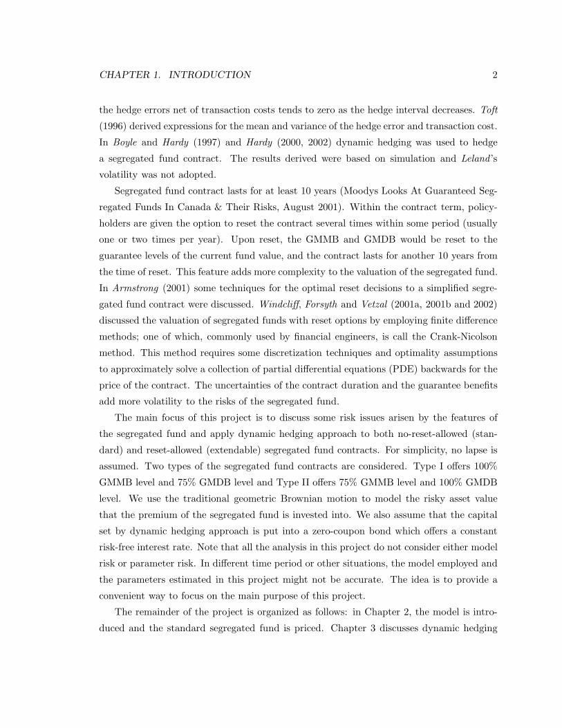
Figure 3.1 shows the hedge errors net of the transaction costs at each hedge time based
on annual, monthly, weekly and daily hedge strategies, respectively. The solid lines represent
the costs based on σ and the dotted lines correspond with Leland ’s volatility. The same put
option as above is assumed. The costs are lower for Leland ’s volatility and are almost zero
for the monthly hedge. The sharp changes at the end of the term reflect the relatively large
amount of the traded asset shares.
Note that for a segregated fund contract, annual charges may make the total hedge errors
net of transaction costs not strictly decreasing as the hedge frequency increases. However,
Table 3.3: The hedge errors net of the transaction costs with σ. The annual charge isdeducted
Annual charge rate Annually Monthly Weekly Daily
1% -0.5726 -1.5372 -3.1628 -8.35712% -0.6310 -1.7188 -3.5372 -9.34613% -0.6708 -1.8519 -3.8120 -10.0721
CHAPTER 3. DYNAMIC HEDGING APPROACH 14
Table 3.4: The hedge errors net of the transaction costs with σ. The annual charge isdeducted
Annual charge rate Annually Monthly Weekly Daily
1% -0.1776 -0.1637 -0.2917 -0.67802% -0.2300 -0.3237 -0.6081 -1.42573% -0.2789 -0.4875 -0.9335 -2.1970
2 4 6 8 10
−0.0
8−0
.06
−0.0
4−0
.02
0.00
Annually
Time
Cos
ts
0 2 4 6 8 10
−0.0
8−0
.06
−0.0
4−0
.02
0.00
Monthly
Time
Cos
ts
0 2 4 6 8 10
−0.0
8−0
.06
−0.0
4−0
.02
0.00
Weekly
Time
Cos
ts
0 2 4 6 8 10
−0.0
8−0
.06
−0.0
4−0
.02
0.00
Daily
Time
Cos
ts
Figure 3.1: The hedge errors net of the transaction costs at each hedge time

CHAPTER 3. DYNAMIC HEDGING APPROACH 15
Leland ’s volatility still has a positive effect on the hedge costs. As shown in Tables 3.3 and
3.4, from annual to daily hedge, the total hedge errors net of the transaction costs with σ
increase up to about fifteen times, while they only increase by three times for 1% of the
annual charge rate and seven times for 3% of the annual charge rate under the effect of
Leland ’s volatility.
3.3 Hedging for the segregated fund contract
3.3.1 The initial hedge cost
The hedge cost for the segregated fund contract includes two parts: the cost to set up the
hedging portfolio (HP cost) and the hedge error net of the transaction cost (H&T) reserve.
The HP cost is determined by the modified Black-Scholes European put option formula
incorporating Leland ’s volatility. Assuming deaths can only occur at the end of the year,
the formula for the HP cost is
MP =
T−1∑
j=0
P (S0(1 − m)T , Gd, 0, j + 1) · j|qx
+P (S0(1 − m)T , Gm, 0, T ) · T px, (3.9)
where Gm and Gd represent the GMMB and GMDB guarantees, respectively, and MP de-
notes the initial hedge cost for the $Gm GMMB and $Gd GMDB contract for a policyholder
aged x at time 0 with asset price S0. Equation (3.9) states that the HP cost for the seg-
regated fund contract consists of a collection of hedging portfolios whose initial values are
defined in Equation (2.3) incorporating Leland ’s volatility with different durations. There-
fore, to fund the H&T reserve, we should calculate the expected present value of total hedge
errors net of the transaction costs for each of those hedge portfolios. Let 0V(H&T )T denote
the H&T reserve for a T-year contract at time 0, then
0V(H&T )T =
T−1∑
j=0
Ψ(0, j + 1) · j|qx + Ψ(0, T ) · T px. (3.10)
When applying Equation (3.10) the charges should be taken into account. That is, the
annual charge should be deducted from the segregated fund before the hedging portfolio is
modified at each integer year. Figures 3.2, 3.3 and 3.4 show some numerical results based
on annual, monthly and weekly hedge strategies, respectively, for a ten-year contract with a

CHAPTER 3. DYNAMIC HEDGING APPROACH 16
Age
20
40
60
80
Cha
rge
0.000
0.005
0.010
0.015
0.020
0.025
0.030
Hedge cost for G
MM
B
0
5
10
15
20
25
Age
20
40
60
80
Cha
rge
0.000
0.005
0.010
0.015
0.020
0.025
0.030H
edge cost for GM
MB
0
5
10
15
20
25
Age
20
40
60
80
Cha
rge
0.000
0.005
0.010
0.015
0.020
0.025
0.030
Hedge cost for G
MD
B
0
5
10
15
20
25
Age
20
40
60
80
Cha
rge
0.000
0.005
0.010
0.015
0.020
0.025
0.030
Hedge cost for G
MD
B
0
5
10
15
20
25
Age
20
40
60
80
Cha
rge
0.000
0.005
0.010
0.015
0.020
0.025
0.030
Total hedge cost
0
5
10
15
20
25
Age
20
40
60
80
Cha
rge
0.000
0.005
0.010
0.015
0.020
0.025
0.030
Total hedge cost
0
5
10
15
20
25
Figure 3.2: The initial hedge costs for the annually hedging strategy

CHAPTER 3. DYNAMIC HEDGING APPROACH 17
Age
20
40
60
80
Cha
rge
0.000
0.005
0.010
0.015
0.020
0.025
0.030
Hedge cost for G
MM
B
0
5
10
15
20
25
Age
20
40
60
80
Cha
rge
0.000
0.005
0.010
0.015
0.020
0.025
0.030H
edge cost for GM
MB
0
5
10
15
20
25
Age
20
40
60
80
Cha
rge
0.000
0.005
0.010
0.015
0.020
0.025
0.030
Hedge cost for G
MD
B
0
5
10
15
20
25
Age
20
40
60
80
Cha
rge
0.000
0.005
0.010
0.015
0.020
0.025
0.030
Hedge cost for G
MD
B
0
5
10
15
20
25
Age
20
40
60
80
Cha
rge
0.000
0.005
0.010
0.015
0.020
0.025
0.030
Total hedge cost
0
5
10
15
20
25
Age
20
40
60
80
Cha
rge
0.000
0.005
0.010
0.015
0.020
0.025
0.030
Total hedge cost
0
5
10
15
20
25
Figure 3.3: The initial hedge costs for the monthly hedging strategy

CHAPTER 3. DYNAMIC HEDGING APPROACH 18
Age
20
40
60
80
Cha
rge
0.000
0.005
0.010
0.015
0.020
0.025
0.030
Hedge cost for G
MM
B
0
5
10
15
20
25
Age
20
40
60
80
Cha
rge
0.000
0.005
0.010
0.015
0.020
0.025
0.030H
edge cost for GM
MB
0
5
10
15
20
25
Age
20
40
60
80
Cha
rge
0.000
0.005
0.010
0.015
0.020
0.025
0.030
Hedge cost for G
MD
B
0
5
10
15
20
25
Age
20
40
60
80
Cha
rge
0.000
0.005
0.010
0.015
0.020
0.025
0.030
Hedge cost for G
MD
B
0
5
10
15
20
25
Age
20
40
60
80
Cha
rge
0.000
0.005
0.010
0.015
0.020
0.025
0.030
Total hedge cost
0
5
10
15
20
25
Age
20
40
60
80
Cha
rge
0.000
0.005
0.010
0.015
0.020
0.025
0.030
Total hedge cost
0
5
10
15
20
25
Figure 3.4: The initial hedge costs for the weekly hedging strategy

CHAPTER 3. DYNAMIC HEDGING APPROACH 19
single premium $100. The graphs on the left hand side are for Type I contracts and those on
the right hand side for Type II contracts. We first note that for Type I contracts the initial
hedge costs for the GMMB dominate the total hedge costs for relatively young policyholders.
In the case of Type II contracts the initial hedge costs for the GMDB dominate the total
hedge costs when the policyholder is relatively old, which leads to relatively high total hedge
costs for the contracts. Second, for Type I contracts the change of the charges has much
effect on the total hedge cost for relatively young policyholders. This is mainly because of
the 100% GMMB offered by Type I contracts. The charge deduction could be considered
as a negative return on the segregated fund. As the charge increases, it is more likely that
the fund at maturity stays below the initial deposit. The increasing chance of the positive
payoff calls for higher hedge costs from the insurance company.
3.3.2 Re-balancing the hedging portfolio
As we mentioned earlier, after the initial hedge cost is calculated, periodical re-balancing
of the hedging portfolio is needed until the contract matures. The balancing frequency
depends on the hedge strategy. Given a hedge time tj, where T ≥ tj > 0, based on newly
gathered information at time tj , denoted by Itj (i.e. the asset price Stj and policyholders
who are still alive lx+tj ), the revised HP cost and H&T reserve for the revised portfolio at
time t1 are
MP |Itj =
T−tj−1∑
J=0
P (Stj (1 − m)T , Gd, tj, tj + J + 1) · J |qx+tj · lx+tj
+P (Stj (1 − m)T , Gm, tj , T ) · T−tjpx+tj · lx+tj (3.11)
and
tjV(H&T )T |Itj =
T−tj−1∑
J=0
Ψ(tj , tj + J + 1) · J |qx+tj · lx+t1
+Ψ(tj , T ) · T−tjpx+tj · lx+tj . (3.12)
respectively.
Results of the hedge cost movement during the lifetime of the contracts from Equations
(3.11) and (3.12) are shown From Figures 3.5 to 3.10. The simulated asset prices used are
from four types of asset price paths in Figure 2.1. We assume that the annual charge rate
m = 1% and a pool of 100 insureds whose ages are all 30, 60 and 80 respectively with $1 put

CHAPTER 3. DYNAMIC HEDGING APPROACH 20
0 2 4 6 8 10
010
2030
4050
6070
Age 30Time
Hed
ge c
ost
0 2 4 6 8 10
010
2030
4050
6070
Age 30Time
Hed
ge c
ost
0 2 4 6 8 10
010
2030
4050
6070
Age 30Time
Hed
ge c
ost
0 2 4 6 8 10
010
2030
4050
6070
Age 30Time
Hed
ge c
ost
Figure 3.5: Type I, Age 30, $100 single premium

CHAPTER 3. DYNAMIC HEDGING APPROACH 21
0 2 4 6 8 10
010
2030
4050
6070
Age 60Time
Hed
ge c
ost
0 2 4 6 8 10
010
2030
4050
6070
Age 60Time
Hed
ge c
ost
0 2 4 6 8 10
010
2030
4050
6070
Age 60Time
Hed
ge c
ost
0 2 4 6 8 10
010
2030
4050
6070
Age 60Time
Hed
ge c
ost
Figure 3.6: Type I, Age 60, $100 single premium

CHAPTER 3. DYNAMIC HEDGING APPROACH 22
0 2 4 6 8 10
010
2030
4050
6070
Age 80Time
Hed
ge c
ost
0 2 4 6 8 10
010
2030
4050
6070
Age 80Time
Hed
ge c
ost
0 2 4 6 8 10
010
2030
4050
6070
Age 80Time
Hed
ge c
ost
0 2 4 6 8 10
010
2030
4050
6070
Age 80Time
Hed
ge c
ost
Figure 3.7: Type I, Age 80, $100 single premium

CHAPTER 3. DYNAMIC HEDGING APPROACH 23
0 2 4 6 8 10
010
2030
4050
6070
Age 30Time
Hed
ge c
ost
0 2 4 6 8 10
010
2030
4050
6070
Age 30Time
Hed
ge c
ost
0 2 4 6 8 10
010
2030
4050
6070
Age 30Time
Hed
ge c
ost
0 2 4 6 8 10
010
2030
4050
6070
Age 30Time
Hed
ge c
ost
Figure 3.8: Type II, Age 30, $100 single premium

CHAPTER 3. DYNAMIC HEDGING APPROACH 24
0 2 4 6 8 10
010
2030
4050
6070
Age 60Time
Hed
ge c
ost
0 2 4 6 8 10
010
2030
4050
6070
Age 60Time
Hed
ge c
ost
0 2 4 6 8 10
010
2030
4050
6070
Age 60Time
Hed
ge c
ost
0 2 4 6 8 10
010
2030
4050
6070
Age 60Time
Hed
ge c
ost
Figure 3.9: Type II, Age 60, $100 single premium

CHAPTER 3. DYNAMIC HEDGING APPROACH 25
0 2 4 6 8 10
010
2030
4050
6070
Age 80Time
Hed
ge c
ost
0 2 4 6 8 10
010
2030
4050
6070
Age 80Time
Hed
ge c
ost
0 2 4 6 8 10
010
2030
4050
6070
Age 80Time
Hed
ge c
ost
0 2 4 6 8 10
010
2030
4050
6070
Age 80Time
Hed
ge c
ost
Figure 3.10: Type II, Age 80, $100 single premium

CHAPTER 3. DYNAMIC HEDGING APPROACH 26
into Type I or Type II segregated fund contracts. The solid lines represent the results from
monthly hedge strategy; the dashed lines represent weekly hedge results and the dotted lines
are for the annual ones. In general, The hedge cost is reduce when the asset price raises and
increased for the drop of the asset price. For example, in graphs at the top left, the asset
price increases to a relatively high level after year 6. As a result, the hedge cost is gradually
reduced to zero. For another example, the poor investment in the top right graphs makes
the segregated fund deep in the money. In turn, a relatively high hedge cost is required. It
should also be noted that under the annual hedge strategy the hedge portfolio is adjusted
only at the end of each year. It ignores many details of the asset price fluctuation within
each year. As a result, we would expect relatively large cash flow volatility.
3.4 The cash flows
To analyze the effect of the dynamic hedging approach on the segregated, the loss or profit
of the insurance company needs to be studied. cash flows are projected based on the incomes
and outgoes from the company. For the segregated fund, the cash flows include the charge
incomes and benefit payments. Under the dynamic hedging approach, it also involves cost
for the hedge errors and transaction costs. Assuming that each policyholder puts $1 into
the segregated fund, at the beginning of the 10-year contract, the net cash flow is the initial
hedge cost net of the initial charge. Let CFt denote the net cash flow at time t, then,
CF0 = lx
(m − MP − 0V
(H&T )10
).
During the lifetime of the contract, the net cash flows are a bit complicated. The composition
of the cash flows for year t = 1, 2, . . . , 9 can be seen in Table 3.5. For further analysis, we
decompose the cash flows into four parts for year t = 1, 2, . . . , 9. The first part is the annual
charge applicable to policyholders who are still alive at the beginning of year t+1. The
income of the second part is the projection of the initial hedge cost from year t-1 to t,
denoted by
MP (p)|It−1 =
10−t∑
j=0
H−(Gd, t − 1, t + j) · j|qx+t−1 · lx+t−1
+H−(Gm, 11 − t, T ) · 11−tpx+t−1 · lx+t−1,
where
H−(G, τ1, τ2) = Ge−r(τ2−τ1−1)Φ(−d2(G, τ1, τ2)) − Sτ1+1Φ(−d1(G, τ1, τ2))

CHAPTER 3. DYNAMIC HEDGING APPROACH 27
Table 3.5: The cash flows in the mid-years
Part Income Outgo Net cash flow
A lx+tSt · (1 − m)t · m lx+tSt · (1 − m)t · m
B MP (p)|It−1 MP |It
(lx+t−1 − lx+t)L(Gd, t) HE(act)t
C HT (act)t −HT (act)
t
D(
t−1V(H&T )10 |It−1
)er
tV(H&T )10 |It RE t
d1(G, τ1, τ2) =log
Sj(1−m)τ2
G + (r + 12 σ2)(τ2 − τ1)
σ√
τ2 − τ1,
and
d2(G, τ1, τ2) = d1(G, τ1, τ2) − σ√
τ2 − τ1
for τ2 = τ1 + 1, . . . , 10. The outgoes of the second part consist of two components: one is
the revised initial hedge cost based on the information at year t, MP |It; the other is the
payoff of the GMDB from the actually terminated contracts at the end of year t. Then the
net cash flow (defined as the actual hedge error) occurring at the end of year t is denoted
by
HE(act)t = MP (p)|It−1 − MP |It − (lx+t−1 − lx+t)L(Gd, t).
For the third part, we recognize the hedging transaction costs for both terminated and valid
contracts at the end of year t as
HT (act)t = 0.005 × St
{|Φ(−d1(Gd, t, t)) − Φ(−d1(Gd, t − 1, t))| · (lx+t−1 − lx+t)
+9−t∑
j=0
|Φ(−d1(Gd, t, t + j + 1)) − Φ(−d1(Gd, t − 1, t + j + 1))| · j|qx+t · lx+t
+ |Φ(−d1(Gm, t, 10)) − Φ(−d1(Gm, t − 1, 10))| · 10−tpx+t · lx+t
}.
The last part is defined as H&T reserve error at year t, RE t. It is the difference between the
projection of H&T reserve from year t-1 to t,(
t−1V(H&T )10 |It−1
)er, and the H&T reserve

CHAPTER 3. DYNAMIC HEDGING APPROACH 28
needed at year t, tV(H&T )10 |It.
To sum up, we write the net cash flow at the end of year t (t = 1, 2, . . . , 9) as
CFt = lx+tSt · (1 − m)t · m + HE(act)t −HT (act)
t + RE t.
Similarly, the cash flow at the end of the last year is
CF10 = MP (p)|I9 − (lx+t−1 − lx+t)L(Gd, 10) − lx+tL(Gm, 10) −HT (act)10 .
It should be noted for the monthly and weekly hedging strategies, net cash flows at fraction
year need to be considered. They are similar to those at integer year. The difference is:
Part A in Table 3.5 is zero since charge is deducted at the beginning of each year; based on
the assumption of GMDB is payable at the end of the year, there is no GMDB payoff or
transaction costs for GMDB payoff.
Figures 3.11 to 3.16 show the net cash flows generated by the dynamic hedging ap-
proach, corresponding to the asset price paths in Figure 2.1. For monthly and weekly hedge
strategies those outstanding positive cash flows at the integer years are partially or mostly
attributed to the annual charges. Under the annual hedge strategy, the hedging portfolio is
adjusted only at the end of each year, which general relatively large net cash flows at each
hedge time. On the other hand, portfolio adjustments are also needed within each year.
This leads to relatively smooth cash flows. Specifically, look at the third column in Figure
3.11 which corresponds to graph (c) in Figure 2.1 and the bottom left one in Figure 3.5.
From year 7 to year 8, there is a relatively large return on the fund investment. In turn, the
cash for the hedge cost is released at the end of year 7. However, the large hedging portfolio
adjustment also causes relatively high transaction costs. As a result, a relatively large loss
is generated at the end of year 7 under the annual hedge strategy. On the other hand,
the segregated fund is gradually hedged from year 7 to year 8 under monthly or weekly
strategy. The outstanding loss at the end of year 7 under annual hedge strategy is replaced
with monthly or weekly cash flows within year 7.
The amount of the net cash flow in each year is an important issue. The speed at which
the cash is being released back to the company is another critical issue. The net present
value (NPV) of the cash flows provides a good basis for the analysis of the dynamic hedging
approach. Under the dynamic hedging approach, the NPV of the cash flows can be expressed
as
NPV =
T/∆t∑
j=0
CFj(1 + id)−j∆t,

CHAPTER 3. DYNAMIC HEDGING APPROACH 29
0 2 4 6 8 10
−1
5−
10
−5
0
AnnuallyTime
Ne
t ca
sh flo
w
0 2 4 6 8 10
−1
5−
10
−5
0
AnnuallyTime
Ne
t ca
sh flo
w
0 2 4 6 8 10
−1
5−
10
−5
0
AnnuallyTime
Ne
t ca
sh flo
w
0 2 4 6 8 10
−1
5−
10
−5
0
AnnuallyTime
Ne
t ca
sh flo
w0 2 4 6 8 10
−1
5−
10
−5
0
MonthlyTime
Ne
t ca
sh flo
w
0 2 4 6 8 10
−1
5−
10
−5
0
MonthlyTime
Ne
t ca
sh flo
w
0 2 4 6 8 10
−1
5−
10
−5
0
MonthlyTime
Ne
t ca
sh flo
w
0 2 4 6 8 10
−1
5−
10
−5
0Monthly
Time
Ne
t ca
sh flo
w
0 2 4 6 8 10
−1
5−
10
−5
0
WeeklyTime
Ne
t ca
sh flo
w
0 2 4 6 8 10
−1
5−
10
−5
0
WeeklyTime
Ne
t ca
sh flo
w
0 2 4 6 8 10
−1
5−
10
−5
0
WeeklyTime
Ne
t ca
sh flo
w
0 2 4 6 8 10
−1
5−
10
−5
0
WeeklyTime
Ne
t ca
sh flo
w
Figure 3.11: Net Cash flows of Type I contract, Age 30

CHAPTER 3. DYNAMIC HEDGING APPROACH 30
0 2 4 6 8 10
−1
5−
10
−5
0
AnnuallyTime
Ne
t ca
sh flo
w
0 2 4 6 8 10
−1
5−
10
−5
0
AnnuallyTime
Ne
t ca
sh flo
w
0 2 4 6 8 10
−1
5−
10
−5
0
AnnuallyTime
Ne
t ca
sh flo
w
0 2 4 6 8 10
−1
5−
10
−5
0
AnnuallyTime
Ne
t ca
sh flo
w0 2 4 6 8 10
−1
5−
10
−5
0
MonthlyTime
Ne
t ca
sh flo
w
0 2 4 6 8 10
−1
5−
10
−5
0
MonthlyTime
Ne
t ca
sh flo
w
0 2 4 6 8 10
−1
5−
10
−5
0
MonthlyTime
Ne
t ca
sh flo
w
0 2 4 6 8 10
−1
5−
10
−5
0Monthly
Time
Ne
t ca
sh flo
w
0 2 4 6 8 10
−1
5−
10
−5
0
WeeklyTime
Ne
t ca
sh flo
w
0 2 4 6 8 10
−1
5−
10
−5
0
WeeklyTime
Ne
t ca
sh flo
w
0 2 4 6 8 10
−1
5−
10
−5
0
WeeklyTime
Ne
t ca
sh flo
w
0 2 4 6 8 10
−1
5−
10
−5
0
WeeklyTime
Ne
t ca
sh flo
w
Figure 3.12: Net Cash flows of Type I contract, Age 60

CHAPTER 3. DYNAMIC HEDGING APPROACH 31
0 2 4 6 8 10
−1
5−
10
−5
0
AnnuallyTime
Ne
t ca
sh flo
w
0 2 4 6 8 10
−1
5−
10
−5
0
AnnuallyTime
Ne
t ca
sh flo
w
0 2 4 6 8 10
−1
5−
10
−5
0
AnnuallyTime
Ne
t ca
sh flo
w
0 2 4 6 8 10
−1
5−
10
−5
0
AnnuallyTime
Ne
t ca
sh flo
w0 2 4 6 8 10
−1
5−
10
−5
0
MonthlyTime
Ne
t ca
sh flo
w
0 2 4 6 8 10
−1
5−
10
−5
0
MonthlyTime
Ne
t ca
sh flo
w
0 2 4 6 8 10
−1
5−
10
−5
0
MonthlyTime
Ne
t ca
sh flo
w
0 2 4 6 8 10
−1
5−
10
−5
0Monthly
Time
Ne
t ca
sh flo
w
0 2 4 6 8 10
−1
5−
10
−5
0
WeeklyTime
Ne
t ca
sh flo
w
0 2 4 6 8 10
−1
5−
10
−5
0
WeeklyTime
Ne
t ca
sh flo
w
0 2 4 6 8 10
−1
5−
10
−5
0
WeeklyTime
Ne
t ca
sh flo
w
0 2 4 6 8 10
−1
5−
10
−5
0
WeeklyTime
Ne
t ca
sh flo
w
Figure 3.13: Net Cash flows of Type I contract, Age 80

CHAPTER 3. DYNAMIC HEDGING APPROACH 32
0 2 4 6 8 10
−1
5−
10
−5
0
AnnuallyTime
Ne
t ca
sh flo
w
0 2 4 6 8 10
−1
5−
10
−5
0
AnnuallyTime
Ne
t ca
sh flo
w
0 2 4 6 8 10
−1
5−
10
−5
0
AnnuallyTime
Ne
t ca
sh flo
w
0 2 4 6 8 10
−1
5−
10
−5
0
AnnuallyTime
Ne
t ca
sh flo
w0 2 4 6 8 10
−1
5−
10
−5
0
MonthlyTime
Ne
t ca
sh flo
w
0 2 4 6 8 10
−1
5−
10
−5
0
MonthlyTime
Ne
t ca
sh flo
w
0 2 4 6 8 10
−1
5−
10
−5
0
MonthlyTime
Ne
t ca
sh flo
w
0 2 4 6 8 10
−1
5−
10
−5
0Monthly
Time
Ne
t ca
sh flo
w
0 2 4 6 8 10
−1
5−
10
−5
0
WeeklyTime
Ne
t ca
sh flo
w
0 2 4 6 8 10
−1
5−
10
−5
0
WeeklyTime
Ne
t ca
sh flo
w
0 2 4 6 8 10
−1
5−
10
−5
0
WeeklyTime
Ne
t ca
sh flo
w
0 2 4 6 8 10
−1
5−
10
−5
0
WeeklyTime
Ne
t ca
sh flo
w
Figure 3.14: Net Cash flows of Type II contract, Age 30

CHAPTER 3. DYNAMIC HEDGING APPROACH 33
0 2 4 6 8 10
−1
5−
10
−5
0
AnnuallyTime
Ne
t ca
sh flo
w
0 2 4 6 8 10
−1
5−
10
−5
0
AnnuallyTime
Ne
t ca
sh flo
w
0 2 4 6 8 10
−1
5−
10
−5
0
AnnuallyTime
Ne
t ca
sh flo
w
0 2 4 6 8 10
−1
5−
10
−5
0
AnnuallyTime
Ne
t ca
sh flo
w0 2 4 6 8 10
−1
5−
10
−5
0
MonthlyTime
Ne
t ca
sh flo
w
0 2 4 6 8 10
−1
5−
10
−5
0
MonthlyTime
Ne
t ca
sh flo
w
0 2 4 6 8 10
−1
5−
10
−5
0
MonthlyTime
Ne
t ca
sh flo
w
0 2 4 6 8 10
−1
5−
10
−5
0Monthly
Time
Ne
t ca
sh flo
w
0 2 4 6 8 10
−1
5−
10
−5
0
WeeklyTime
Ne
t ca
sh flo
w
0 2 4 6 8 10
−1
5−
10
−5
0
WeeklyTime
Ne
t ca
sh flo
w
0 2 4 6 8 10
−1
5−
10
−5
0
WeeklyTime
Ne
t ca
sh flo
w
0 2 4 6 8 10
−1
5−
10
−5
0
WeeklyTime
Ne
t ca
sh flo
w
Figure 3.15: Net Cash flows of Type II contract, Age 60

CHAPTER 3. DYNAMIC HEDGING APPROACH 34
0 2 4 6 8 10
−1
5−
10
−5
0
AnnuallyTime
Ne
t ca
sh flo
w
0 2 4 6 8 10
−1
5−
10
−5
0
AnnuallyTime
Ne
t ca
sh flo
w
0 2 4 6 8 10
−1
5−
10
−5
0
AnnuallyTime
Ne
t ca
sh flo
w
0 2 4 6 8 10
−1
5−
10
−5
0
AnnuallyTime
Ne
t ca
sh flo
w0 2 4 6 8 10
−1
5−
10
−5
0
MonthlyTime
Ne
t ca
sh flo
w
0 2 4 6 8 10
−1
5−
10
−5
0
MonthlyTime
Ne
t ca
sh flo
w
0 2 4 6 8 10
−1
5−
10
−5
0
MonthlyTime
Ne
t ca
sh flo
w
0 2 4 6 8 10
−1
5−
10
−5
0Monthly
Time
Ne
t ca
sh flo
w
0 2 4 6 8 10
−1
5−
10
−5
0
WeeklyTime
Ne
t ca
sh flo
w
0 2 4 6 8 10
−1
5−
10
−5
0
WeeklyTime
Ne
t ca
sh flo
w
0 2 4 6 8 10
−1
5−
10
−5
0
WeeklyTime
Ne
t ca
sh flo
w
0 2 4 6 8 10
−1
5−
10
−5
0
WeeklyTime
Ne
t ca
sh flo
w
Figure 3.16: Net Cash flows of Type II contract, Age 80

CHAPTER 3. DYNAMIC HEDGING APPROACH 35
where id is the annual interest rate to discount the cash flows.
The mean and standard deviation of the simulated NPV of the cash flows are shown in
Figure 3.17. A Policyholder aged 30 with $100 single premium Type I contract is chosen.
Under the dynamic hedging approach, the NPV of the cash flows with higher annual charge
and lower discount rate are subject to greater mean and standard deviation. On the other
hand, however, with the help of the dynamic hedging, the NPV of the cash flows is rela-
tively insensitive to both interest rate and charge rate. Specifically, monthly hedge strategy
generates relatively small standard deviation, which indicates better effect on controlling
the risk volatility as more asset price details are captured.
To help further analyze the dynamic hedging approach, the simulated distribution and
the percentiles of the NPV of the cash flows are shown in Figures 3.18 and 3.19. Type I
contract is chosen. Annual charge rate and interest rate for discount are assumed to be 1%
and r respectively. The solid line represents the one without dynamic hedging which has a
long left tail. The segregated fund has a positive mean (1.9922) and a standard deviation
of 15.4465. As derived in Chapter Two, the actuarial solution of the annual charge is about
0.75%. The 0.25% surcharge in our example may be attributed to the average surplus of
the segregated fund. The curve for the dynamic hedging approach, on the other hand, is
more concentrated. The mean and standard deviation are -3.7828 and 3.2641 respectively.
In Figure 3.19, we can see that without a dynamic hedging approach, there is a 20% chance
of generating quite poor NPV of the cash flows, while for most of the time the NPV of the
cash flows ends up within the range from 0 to -20 under monthly hedging strategy. For
the dynamic hedge approach, both figures do not indicate a high chance of getting positive
NPV since transaction costs are involved in the hedge strategy and 1% per year may be
not sufficient enough to cover both guarantees and transaction costs. However, they reveal
that dynamic hedging approach is in favor of reducing the left tail and volatility of the
distribution.

CHAPTER 3. DYNAMIC HEDGING APPROACH 36
Interest rate
0.00
0.05
0.10
0.15
Cha
rge
0.000
0.005
0.010
0.015
0.0200.025
0.030
Mean
−30
−20
−10
0
10
20
Annual hedge
Interest rate
0.00
0.05
0.10
0.15
Cha
rge
0.000
0.005
0.010
0.015
0.0200.025
0.030
Mean
−30
−20
−10
0
10
20
Monthly hedge
Interest rate
0.00
0.05
0.10
0.15
Cha
rge
0.000
0.005
0.010
0.015
0.0200.025
0.030
Sandard deviation
0
5
10
15
20
Annual hedge
Interest rate
0.00
0.05
0.10
0.15
Cha
rge
0.000
0.005
0.010
0.015
0.0200.025
0.030
Sandard deviation
0
5
10
15
20
Monthly hedge
Figure 3.17: The mean and standard deviation of the NPV of the cash flows. Type I, Age30 and $100 single premium contract is used

CHAPTER 3. DYNAMIC HEDGING APPROACH 37
−60 −40 −20 0 20
0.00
0.02
0.04
0.06
0.08
0.10
0.12
NPV of the cash flows
Den
sity
Segregated fund
Monthly hedging
Figure 3.18: Comparison of the distributions of the NPV of the cash flows
0.0 0.2 0.4 0.6 0.8 1.0
−60
−40
−20
020
Percentile
Qua
ntile
Segregated fund
Monthly hedge
Figure 3.19: Comparison of the percentiles of the NPV of the cash flows

Chapter 4
Valuation of the reset option
Segregated funds may have reset options allowing the policyholders to lock in the investment
gains several times per year (http://www.segfundscanada.ca). Once the contract gets reset,
the guarantee levels are based on the current fund level and the term of the contract is
extended to another 10 years. The reset option adds some complications to the valuation
of the segregated fund since both the guarantees and the maturity date are uncertain.
Windcliff, Forsyth and Vetzal (2001a, 2001b) discussed a approach to price extendable
segregated fund by employing some finite difference methods. In this project, we do not go
that far since it needs both a large amount of time and some high speed computer. We only
borrow the spirit of this approach and use a simplified case to demonstrate the main idea
and further price the added value of the reset option.
4.1 Introduction of Crank-Nicolson method
4.1.1 Discretization techniques
Crank-Nicolson method is one of the implicit finite difference methods solving Black-Scholes
PDE numerically for the price of the derivative securities (Back (2005)). For simplicity, we
use short notations S and P to represent the asset price at time t and the European put
price at time t with asset price S, respectively. The PDE is shown by
∂P
∂t+
1
2σ2S2 ∂2P
∂S2+ rS
∂P
∂S− rP = 0, (4.1)
where 0 ≤ t ≤ T and 0 ≤ S ≤ ∞. The price of the European put option P is a continuous
function of t and S, denoted by V (S, t) (i.e. P = V (S, t)). If ∂t ≈ ∆t and ∂S ≈ ∆S for
38

CHAPTER 4. VALUATION OF THE RESET OPTION 39
some infinitesimal values of ∆t and ∆S as shown in Figure 4.1, the approximate value of P
is denoted by
Vi,n = V (i∆S, n∆t) .
Crank-Nicolson method assumes the existence of the value of P between two grid points
(n∆t, i∆S) and ((n + 1)∆t, i∆S) (Back (2005)). Let V ′i,n denote the Crank-Nicolson value
of P , then
P ≈ V ′i,n =
Vi,n + Vi,n+1
2.
The derivatives in Equation (4.1) are approximately written as
∂P
∂S≈
V ′i+1,n − V ′
i−1,n
2∆S
=Vi+1,n − Vi−1,n + Vi+1,n+1 − Vi−1,n+1
4∆S,
∂2P
∂S2≈
(V ′
i+1,n − V ′i,n
)−(V ′
i,n − V ′i−1,n
)
(∆S)2
=Vi+1,n − 2Vi,n + Vi−1,n + Vi+1,n+1 − 2Vi,n+1 + Vi−1,n
2(∆S)2
and
Pt ≈Pi,n+1 − Pi,n
∆t.
If we let g = ∆t and h = ∆S, Equation (4.1) can be approximately written as
a(i)Pi+1,n + b(i)Pi,n + c(i)Pi−1,n = d(i), (4.2)
where
a(i) = −σ2S(i)2
4h2− rS(i)
4h,
b(i) =1
g+
σ2S(i)2
2h2+
r
2,
c(i) =rS(i)
4h− σ2S(i)2
4h2,
d(i) = −a(i)Pi+1,n+1 +
(1
g− σ2S(i)2
2h2− r
2
)Pi,n+1 − c(i)Pi−1,n+1,
and S(i) denotes the value of S at point i∆S.

CHAPTER 4. VALUATION OF THE RESET OPTION 40
4.1.2 Solving the PDE
As long as we know the values of Pi+1,n+1, Pi,n+1 and Pi−1,n+1, the value of Pi+1,n, Pi,n and
Pi−1,n can be implicitly derived. As shown in Figure 4.1, assuming a relatively large value
Smax to represent the case S → ∞, we discretize S from 0 to Smax to get N intervals such
that Smax = N∆S. Similarly, we disretize t to M intervals such that T = M∆t. At each
time step, N + 1 equations similar to Equation (4.2) (with N + 1 discretized asset price
from 0 to Smax) could be used to solve backward for a collection of P values at those grid
points (i.e., P0,n, P1,n, . . . , PN,n). Repeating this algorithm M times gives the price of the
European put option at time 0 with the desirable asset price, say S∗.
To make this recursive algorithm work, firstly, we need to set the initial values of P ’s at
maturity time T at which the payoffs of the options are made. That is
Pi,M = max (K − S(i), 0) ,
where K is the strike and i = 0, 1, . . . , N .
Secondly, The first and the last of the N +1 equations approximately represent the cases
S → 0 and S → ∞. Plugging the boundary values of S into equation (4.1), we get
Pt =
{rP, if S → 0;
0, if S → ∞.
This gives us the frist equation
(1
k+
r
2
)Pi,n =
(1
k− r
2
)Pi,n+1
with S = 0, and
Pi,n = Pi,n+1
with S = Smax.
The value of ∆S and ∆t are quite critical. It also matters to choose the value Smax to be
far away enough from the desirable asset price. As shown in Table 4.1, for the at-the-money
European put option with the strike equal to $100, setting Smax four times as large as the
strike, together with at least 3000 asset grids, the values derived via the Crank-Nicolson
method converge quite well.

CHAPTER 4. VALUATION OF THE RESET OPTION 41
dsd
sd
sd
sd
sd
aa
nd
d
ad
afa
d
∆ tt=0 t=TS=0
∆S
S*
Pi+1,n+1
Pi,n+1
Pi−1,n+1
Pi+1,n
Pi,n
Pi−1,n
S=∞
Figure 4.1: Discretization of the Black-Scholes pde
Table 4.1: Solving for European put options with 1000 time grids
S gridsBlack-Scholes 1000 3000 3500
Smax = 400 10.05832 10.05818 10.05830 10.05831Smax = 300 10.05832 10.07221 10.05822 10.08268Smax = 200 10.05832 10.01914 10.01897 10.01870

CHAPTER 4. VALUATION OF THE RESET OPTION 42
4.2 Pricing the segregated fund with reset option
As mentioned in Chapter 2, the present value of future charges can be modeled via an
indifference principle. However, reset option makes this approach inapplicable due to the
uncertainties of the benefit amount and maturity date. Following the Black-Scholes PDE,
a more flexible method can be employed. First we make the following assumptions:
• The value of segregated fund is assumed to follows the stochastic differential equation
dSt = (µ − fm)Stdt + σStdBt;
• The value of the segregated fund is a function of the asset price S at time t, guarantee
G, maturity date T and current time t, i.e., P (St, G, t, T );
• The values of G and T upon reset are denoted by G∗ and T ∗, respectively, where
G∗ = αS
and
T ∗ = min(T + 10, Tmax).
α is either 100% or 75%, and Tmax is the maximum maturity date of the segregated
fund. No reset is allowed in the last ten years of Tmax. For simplicity, we only consider
the case that only one reset is allowed per year;
• Upon reset, the value of the segregated fund is denoted by P ∗(St, G, t, T ), where
P ∗(St, G, t, T ) =
{P (St, G
∗, t, T ∗), if reset is allowed;
−∞, otherwise.
4.2.1 Optimality statement
When we solve the equations for the value of the segregated fund with certain value of fm,
we need to compare P with P ∗ at each grid point. From this point of view, the segregated
fund can be considered as a collection of American-type options with different strikes and
maturity dates. Following the standard statements in Wilmott, Dewynne and Howison
(1993), the value of the segregated fund must satisfy
Pt + (r − fm)SPS +1
2σ2S2PSS − rP + D(t)max(Gd − S, 0) − R(t)fmS ≤ 0, (4.3)

CHAPTER 4. VALUATION OF THE RESET OPTION 43
and
P ∗ ≤ P, (4.4)
where one of inequalities (4.3) and (4.4) holds with equality and Gd is the GMDB guarantee.
These two inequalities assume that the policyholders exercise the reset options optimally
without arbitrage and P ∗ can be viewed as the lower bound of P ((4.3) states that the return
from the segregated fund is not greater than the return on the investment to the risk-free
bound. If reset is optimal, (4.4) holds with equality and (4.3) holds with inequality, or vice
versa.). D(t) is defined such that the proportion of the policyholders who die between t and
t + dt is denoted as D(t)dt. R(t) is the proportion of the policyholders who are still alive
at time t, i.e. R(t) = 1 −∫ t0 D(t)dt. In the following, we use a constant force of mortality
in fraction year.
At the end of each year, the number of the used reset is set to zero. The non-arbitrage
statement requires the jump condition
P (St−i, G, t−i , T ) = P (St+i
, G, t+i , T ),
where t−i and t+i represent the moment immediately at the end of the ith year and the
beginning of the i + 1th year, respectively.
4.2.2 Boundary values
The terminal values representing the intrinsic values at time T are
Pi,M = R(T )max (Gm − S(i), 0) , i = 0, 1, . . . , N
where Gm is the GMMB guarantee. The asymptotic condition which reflects the fact that
the asset price goes to 0 or ∞ can be written as
Pt =
{rP − D(t)max(Gd − S, 0), if S → 0;
−D(t)max(Gd − S, 0), if S → ∞.
4.2.3 Implementation
The inequalities (4.3) and (4.4) are three-dimensional (i.e., S, K and T) and time-dependent,
which need very complex computational work. To further programming, we make the
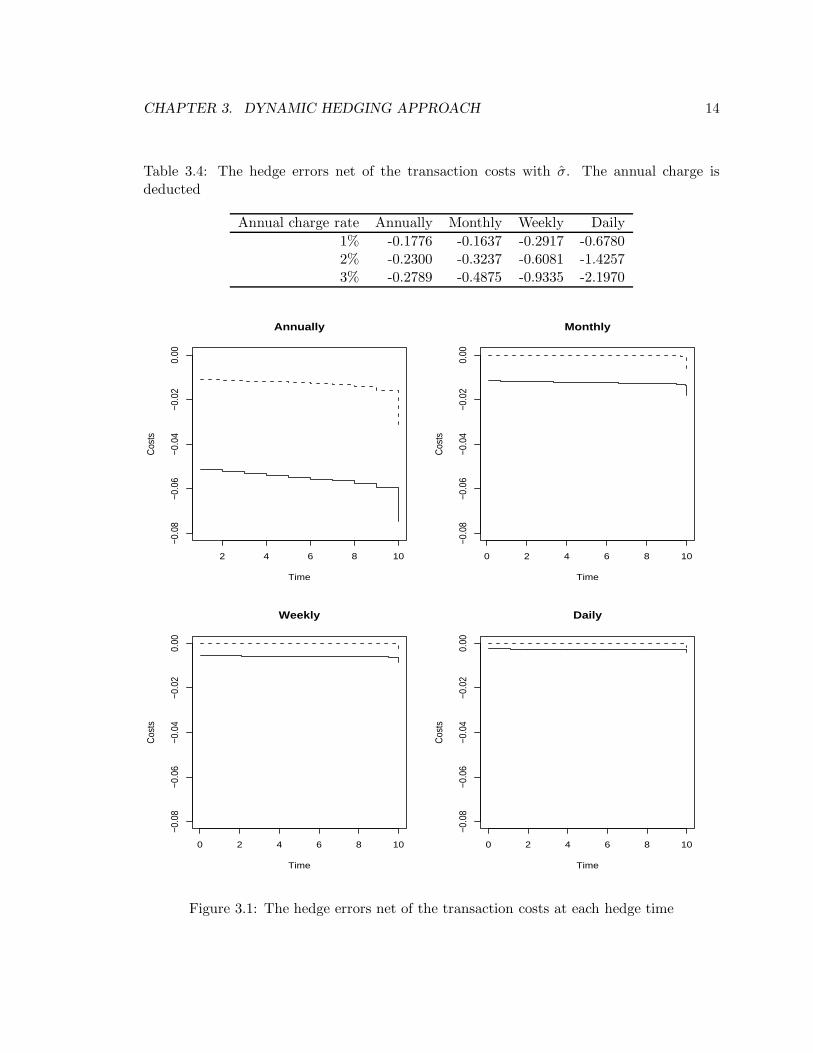
CHAPTER 4. VALUATION OF THE RESET OPTION 44
following simplifications. First, if we let Xi = logS(i), equality (4.3) can be discretized
as
a · Pi+1,n + b · Pi,n + c · Pi−1,n = Z(i), (4.5)
where
a = − σ2
4h2− r − 1
2σ2
4h,
b =1
k+
σ2
2h2+
r
2,
c =r − 1
2σ2
4h− σ2
4h2,
Z(i) = −aPi+1,n+1 +
(1
k− σ2
2h2− r
2
)Pi,n+1 − cPi−1,n+1
+D(t)max(K2 − eXi , 0
)− R(t)fmeXi ,
and i = 1, 2, . . . , N .
The convenience of Equation (4.5) is that all of the N equations except for the first and
the last ones have the same coefficients a, b and c which are independent with Xi. Second,
the maturity date T varies from 10 to 30. Since the length of the contract can only be
extended to anther 10 years upon reset, the possible values of T are constrained by
max(t, 10) ≤ T ≤ min(t + 10, Tmax)
for t from 0 to Tmax. To start the programming, we need to define a three-dimensional
array, say P [DX ][DG][DT ], to represent the collection of American-type options. We set
1001 grids for both S and K dimensions so that h = Smax
1001 = Kmax
1001 , where Smax = Gmax
(Gmax is the maximum guarantee that can be reset to). To avoid interpolation complication,
we set the interval of T as the same as time step ∆t, i.e. g = 112 . Therefore, the maximum
number of the values of T is 120. For the last ten years of contract, the segregated fund
contract is simply a European put option. At time t = Tmax, the number of T is one (i.e., T
can only be Tmax). The number of T’s increases as we solve Equation (4.5) backward until
t = Tmax − 10 where the number of T’s reaches the maximum (i.e. 120).
For 10 ≤ t ≤ Tmax − 10, the number of T’s remains 120. For each time step, we need to
compare the value of P with P ∗. That is,
P [DX ][DG][DT ] = max(P [DX ][DG][DT ], P [DX ][DX ][0])

CHAPTER 4. VALUATION OF THE RESET OPTION 45
for DX = 0, 1, . . . , 1000, DK = 0, 1, . . . , 1000 and DT = 0, 1, . . . , 119. DG = DX means that
GMMB is reset to the current fund value. DT = 0 represents T = 10, DT = 1 represents
T = 10+ 12 and so on. For the first 10 years of the contract, the number of T’s decreases by
one at each time step until t = 0 where the value of T is equal to one which represents the
case that T = 10. At this point, we get the present value of the segregated fund contract
with desirable initial fund value, initial guarantee and initial term of 10 years.
4.2.4 The solution of the charge rate
We choose certain value of fm to solve inequality (4.3) for P at time 0 with initial guarantee
and desirable premium. We can try different fm’s to solve Inequality (4.3) until P approaches
zero so that the instantaneous charge rate fm is obtained. However since the computation
is quite time-consuming, we can alternatively use the linear interpolation method which is
illustrated in Figure 4.2. Some numerical results are displayed in Tables 4.2 and 4.3.
Table 4.2: Instantaneous charge rates of Type I contracts
Equation (2.2) Crank-NicolsonActuarial Risk-neutral Standard Extendable
Age 30 0.7400% 1.5400% 1.5231% 4.4751%Age 60 0.6900% 1.4100% 1.3876% 3.5356%
Table 4.3: Instantaneous charge rates of Type II contracts
Equation (2.2) Crank-NicolsonActuarial Risk-neutral Standard Extendable
Age 30 0.2000% 0.4100% 0.3993% 1.1255%Age 60 0.2800% 0.5400% 0.5280% 2.7609%
From the second and the third columns of those two tables, we can see that the analyt-
ical solutions of instantaneous charge rates based on Equation (2.2) are close to the numer-
ical ones based on Crank-Nicolson method, which confirms the feasibility of this numerical
method. The slight differences may be due to the convergence errors and the interpolation
errors. Comparing the values in the last two columns, we can see that segregated fund
contracts with the reset options are more than twice as valuable as those without the re-
set options. Particularly, more dramatic increase occurs to Type II policyholders aged 60.

CHAPTER 4. VALUATION OF THE RESET OPTION 46
50 100 150 200 250
010
2030
40
Asset value
Pric
e
fm=4%
fm=5%
Figure 4.2: The solution of instantaneous charge rate

CHAPTER 4. VALUATION OF THE RESET OPTION 47
As been pointed out in Chapter 2, Type II contracts are very sensitive to the mortality
risk. The reset options call for longer duration of the contracts, which in turn increase the
mortality risk and make this type of contracts relatively expensive.
4.2.5 Further analysis of the charge rate
One of the assumptions the approach above made is that the policyholders optimally exercise
their reset options. In practice, however, this situation barely happens. In general, the
chance that the rest option is exercised is more or less correlated to the premium level
(With higher premium level, the rest options are more frequently used). But the exercise
of the reset option is also affected by other factors such as investment preferences (One
may only want to hold a segregated fund contract for 10 years so that reset option will
not be used) and time issue (When the investment return hits a historical high level, a
position at year one is more likely to trigger a reset than that at year nine). The charge
rates for the extendable segregated fund contracts in Table 4.2 and 4.3 could be considered
as extreme values (Since in reality people do not reset as frequently as they do in optimal
case, reset option may not be as valuable as those considered above). In the following we
use simulation to further analyze the charge rate for the reset option. In practice a lot
of factors and strategies are involved to consider the exercise of the reset option. In this
project, however, for simplicity we introduce a constant return threshold to trigger the reset
options. Once the return on the premium net of the annual charges goes above the threshold
since the beginning of the contracts or last time the reset option is executed, the reset option
will be exercised if it is still applicable during that period. For the purpose of illustration,
we arbitrarily choose 10% annually compounding (or 0.09531 continuously compounding)
as the threshold and only Type I contracts with reset option are considered. Some more
assumptions are addressed below:
• The instantaneous returns on the premium are simulated monthly by a normal gener-
ator under risk-neutral world (This is to be consistent with the risk-neutral analysis
above). If we let log( Sm
Sm−1) denote the monthly return, then
log
(Sm
Sm−1
)∼ N
(1
12
(r − 1
2σ2
),
1
12σ2
).
• The maximum duration of the contract is 30 years with no rest option allowed during
the last ten years. Only one rest option could be exercised during each year.

CHAPTER 4. VALUATION OF THE RESET OPTION 48
• To take mortality effect into account, a pool of 100 30-year-old policyholders with $1
single premium is considered so that the portfolio is worth $100 before the charge
deduction. The force of interest rate for discount is equal to r. GMDB is payable only
at the end of each month. Mortality decrement in faction year is uniformly distributed.
Three cases with annual charge rates 1.5%, 3.0% and 4.5% respectively are tested based
on a 10,000-run simulation. In Figure 4.3 and Table 4.4 the fund value and GMMB payoff at
the time when the contract matures are examined. The fund value represents the segregated
fund investment performance (net of the charges). Since the annual charge rate could
be considered as the negative annual return rate, increasing the charge rate pulls down
the segregated fund level, which in turn thins the right tail of the distribution and shifts
the distribution leftwards. The GMMB payoff is the cost of the insurance company to
compensate the difference between the fund value and the guarantee if the fund value is
less than the guarantee. The high frequency at value 0 corresponds to the part of the fund
distribution where the fund value is beyond 100. It is consistent with the evolution of the
fund value. With increasing the charge rate, the chance that the fund value ends up less than
100 is increased and the chance that no GMMB payoff is needed is reduced. In Table 4.4
both the mean and standard deviation of the fund value decrease with charge rate from 1.5%
to 4.5%. The mean of the GMMB payoff is around 51 for all three cases. On the other hand,
however, there is a significant drop of the standard deviation, which is due to the exercise
of the reset option. The GMMB payoff varies between 0 and the guarantee. Without reset
option, it is capped with 100. But for the extendable segregated fund contract, the cap is
increased every time upon reset. For the large charge rate like 4.5%, the fund return (net of
the charges) is less likely hit the 10% threshold and the fund is less frequently reset, which
explains the decreasing trend of the standard deviation of the GMMB payoff.
Figure 4.4 and Table 4.5 give further proof that the chance of resetting the fund reduces
with charge rate increasing. The duration stands for the time that the contract matures
and the maturity guarantee is the accumulative GMMB guarantee at the maturity of the
contract. The frequency of the 10-year duration goes up with charge rate increasing. This
corresponds with the frequency of the $100 maturity guarantee. With charge rate 4.5%, it
suggests that the about 38% of the contracts do not reset the fund while the proportion drops
to about 24% if 1.5% is charged annually. Additionally, the distribution of the duration with
charge rate 1.5% displays that some contracts might last up to 30 years while for the 4.5%

CHAPTER 4. VALUATION OF THE RESET OPTION 49
m= 1.5%
Fund
Freq
uenc
y
0 100 200 300 400 500
050
100
150
200
m= 3%
Fund
Freq
uenc
y0 100 200 300 400 500
050
100
150
200
m= 4.5%
Fund
Freq
uenc
y
0 100 200 300 400 500
050
100
150
200
m= 1.5%
GMMB payoff
Freq
uenc
y
0 200 400 600 800
020
040
060
080
010
00
m= 3%
GMMB payoff
Freq
uenc
y
0 200 400 600 800
020
040
060
080
010
00
m= 4.5%
GMMB payoff
Freq
uenc
y
0 200 400 600 800
020
040
060
080
010
00
Figure 4.3: The simulated density distributions of the fund value and GMMB payoff atmaturity
Table 4.4: The sample mean and standard deviation of the fund value and GMMB payoffat maturity
m=1.5% Fund GMMB payoff
Mean 112.4231 51.7606Standard deviation 105.6241 43.7160
m=3.0% Fund GMMB payoff
Mean 87.2771 50.1704Standard deviation 67.3597 34.5005
m=4.5% Fund GMMB payoff
Mean 71.6099 51.5752Standard deviation 45.7719 29.3519

CHAPTER 4. VALUATION OF THE RESET OPTION 50
m= 1.5%
Duration
Freq
uenc
y
10 15 20 25 30
010
0020
0030
0040
00m= 3%
Duration
Freq
uenc
y
10 15 20 25 300
1000
2000
3000
4000
m= 4.5%
Duration
Freq
uenc
y
10 15 20 25 30
010
0020
0030
0040
00
m= 1.5%
Maturity guarantee
Freq
uenc
y
200 400 600 800 1000
010
0020
0030
0040
00
m= 3%
Maturity guarantee
Freq
uenc
y
200 400 600 800 1000
010
0020
0030
0040
00
m= 4.5%
Maturity guarantee
Freq
uenc
y
200 400 600 800 1000
010
0020
0030
0040
00
Figure 4.4: The simulated density distributions of the duration and maturity guarantee
Table 4.5: The sample mean and standard deviation of the duration and maturity guarantee
m=1.5% Duration Maturity guarantee
Mean 14.9766 159.6207Standard deviation 5.3272 95.7484
m=3.0% Duration Maturity guarantee
Mean 13.4161 135.9271Standard deviation 4.1863 60.1120
m=4.5% Duration Maturity guarantee
Mean 12.3631 122.8358Standard deviation 3.2954 40.2140

CHAPTER 4. VALUATION OF THE RESET OPTION 51
case most of the contracts last around 10 to 15 years. This means that the charge rate 4.5%
leads to a less frequency of reset comparing to the case with charge rate 1.5%. Even for
those contracts which are reset, a large proportion only gets reset at early times within the
first 10 years.
In Figure 4.5 and Table 4.6, The maturity payment is the summation of the fund value
and GMMB payoff, and the yield is given by
Yield =
(Maturity payment
100
) 1
Duration
− 1.
The higher the charge rate is, the more likely the fund value is below the guarantee, and
the less likely the reset option is used, which leads to a high chance that the fund matures
with $100 and 0% yield. With a threshold 10%, the illustration above shows that when
the charge rate 1.5%, the fund value ends up with $12 higher than GMMB guarantee in
average. The average payment at maturity is $64 larger than the initial fund value. And the
average yield indicates a annual return of 2.14%. When the charge rate increases to 4.5%, in
average, the fund value at maturity goes below GMMB guarantee by $30 and the maturity
payment drops to $123, which yields an average annual return 1.18%. The result is that
large charge rate sharply offsets the positive return of the fund investment and deteriorates
the fund value when the return is negative. With annual charge deduction of 1.5%, the reset
option might be valuable. However, an annual charge rate of 4.5% significantly pulls down
the fund value and the value of the reset option is decreased.
Table 4.6: The sample mean and standard deviation of the total payment and yield atmaturity
m=1.5% Maturity payement Yield at maturity
Mean 164.1838 0.0214Standard deviation 111.8120 0.0193
m=3.0% Maturity payement Yield at maturity
Mean 137.4475 0.0160Standard deviation 67.4705 0.0166
m=4.5% Maturity payement Yield at maturity
Mean 123.1850 0.0118Standard deviation 43.2121 0.0143

CHAPTER 4. VALUATION OF THE RESET OPTION 52
m= 1.5%
Maturity Payment
Freq
uenc
y
100 200 300 400 500
050
010
0015
00
m= 3%
Maturity Payment
Freq
uenc
y
100 200 300 400 500
050
010
0015
00
m= 4.5%
Maturity Payment
Freq
uenc
y
100 200 300 400 500
050
010
0015
00
m= 1.5%
Yield
Freq
uenc
y
0.00 0.05 0.10 0.15
050
010
0015
00
m= 3%
Yield
Freq
uenc
y
0.00 0.05 0.10 0.15
050
010
0015
00
m= 4.5%
Yield
Freq
uenc
y
0.00 0.05 0.10 0.15
050
010
0015
00
Figure 4.5: The simulated density distributions of the total payment and yield at maturity

CHAPTER 4. VALUATION OF THE RESET OPTION 53
m= 1.5%
NPV of the cash flow
Freque
ncy
−200 0 200 400 600
050
100150
200
m= 3%
NPV of the cash flow
Freque
ncy
−200 0 200 400 600
050
100150
200
m= 4.5%
NPV of the cash flow
Freque
ncy
−200 0 200 400 600
050
100150
200
Figure 4.6: The simulated density distributions of the NPV of the cash flows
Figure 4.6 and Table 4.7 show some statistics of the NPV of the cash flows with different
charge rates. In the sense of pricing, a negative NPV of the cash flow suggests that 1.5%
might not be sufficient while the fund with 4.5% annual charge rate might be deducted
(4.5% might be a reasonable charge rate in the case that reset option is treated optimally
since the segregated fund is frequently reset). The linear interpolation between 2.9% and
3% gives a charge rate of 2.941% which approximately generates a 0 NPV of the cash flows.
In the optimality case that reset frequently occurs, a large charge of 4.5% from the
segregated fund is annually deducted. In the 10%-threshold case, the charge rate is lower,
but the reset strategy is still aggressive and the policy is still expensive. Situations in our
example might not happen in practice. Nevertheless, for the following illustration, 2.94%
is considered as a proper annual charge rate for the segregated fund contract with reset
option.
Table 4.7: The sample mean and standard deviation of the NPV of the cash flows
m=1.5% m=3.0% m=4.5%
Mean -13.0757 0.4222 7.608783Standard deviation 29.8358 33.4193 34.46849

CHAPTER 4. VALUATION OF THE RESET OPTION 54
4.3 Hedging the segregated fund with reset option
Reset option may increase the variation of the benefit payoff and add more risk on the
segregated fund. Due to the uncertainty of the length of the contract and the guarantees,
the GMMB and GMDB payoffs may be significantly increased. Based on the simulation
assumption above, Figure 4.7 displays the distributions and percentiles of both standard and
extendable segregated fund contracts, and their means and standard deviations are shown
in Table 4.8. For the segregated fund without reset option, we use the same assumption
as in Figure 3.18 except we generate the asset price using r instead of µ. From Figure 2.2
the proper charge rate is about 1.5% under risk-neutral method. And the negative mean is
due to the insufficiency of 1% of the annual deduction. For the segregated fund with reset
option, the slightly positive mean may stem from the interpolation and sample error (since
we expect a zero mean).
From the distributions of those two types of contracts, the two side tails from the stan-
dard contract are fatter and longer than those from the extendable contract. Specifically, the
extreme loss of the extendable contract could be up to $200. Along with the larger standard
deviation from the extendable contract, it is evident that reset option adds considerable risk
to the segregated fund.
Table 4.8: The mean and standard deviation of the NPV of the cash flows
Standard extendable
Mean -3.3226 0.0658Standard deviation 18.3270 33.3381
In the following we will illustrate the risk diversification effect of the dynamic hedging
approach. The monthly hedging strategy is employed. At the beginning of the contract, the
hedging strategy is set assuming a standard 10-year segregated fund contract. The hedging
re-balancing mentioned in Chapters Three is used. Every time upon reset, the previous
hedging strategy is terminated. At that point of time, the new capital is established to
support another assumed 10-year hedging processes. Note that we do not hedge the reset
option. The consideration of hedging the reset option is beyond the scope of this project.
Figure 4.8 gives the simulated results of the extendable segregated fund contracts with
or without hedging. The solid lines represent the distribution of the segregated fund without
hedging and the dashed lines represent the distribution of the segregated fund under monthly

CHAPTER 4. VALUATION OF THE RESET OPTION 55
−100 −50 0 50 100
0.00
0.02
0.04
0.06
0.08
NPV of the cash flows
Densi
ty
standard
extendable
0.0 0.2 0.4 0.6 0.8 1.0
−200
020
040
0
Percentile
Quan
tile
standard
extendable
Figure 4.7: The density distributions and percentiles of the NPV of the cash flows
Table 4.9: The mean and standard deviation of the NPV of the cash flows with and withouthedging
Segregated fund Monthly hedging
Mean 0.0658 15.7677Standard deviation 33.3381 23.2407
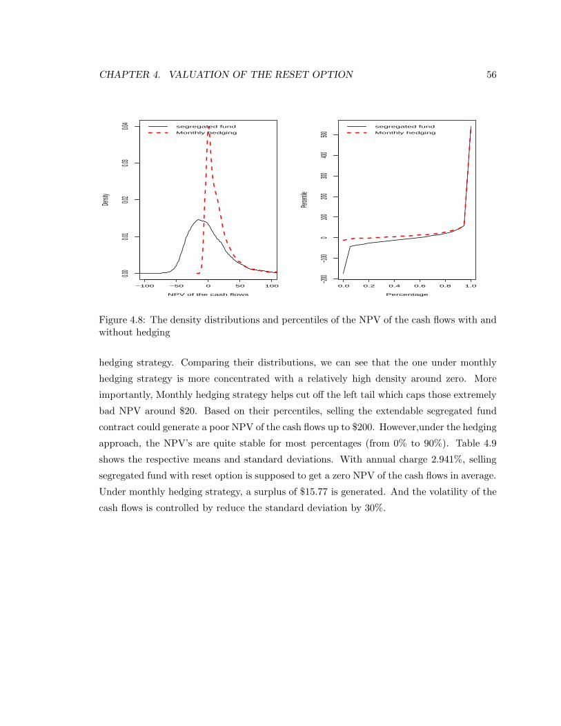
CHAPTER 4. VALUATION OF THE RESET OPTION 56
−100 −50 0 50 100
0.00
0.01
0.02
0.03
0.04
NPV of the cash flows
Density
segregated fund
Monthly hedging
0.0 0.2 0.4 0.6 0.8 1.0
−200
−100
0100
200300
400500
Percentage
Percen
tile
segregated fund
Monthly hedging
Figure 4.8: The density distributions and percentiles of the NPV of the cash flows with andwithout hedging
hedging strategy. Comparing their distributions, we can see that the one under monthly
hedging strategy is more concentrated with a relatively high density around zero. More
importantly, Monthly hedging strategy helps cut off the left tail which caps those extremely
bad NPV around $20. Based on their percentiles, selling the extendable segregated fund
contract could generate a poor NPV of the cash flows up to $200. However,under the hedging
approach, the NPV’s are quite stable for most percentages (from 0% to 90%). Table 4.9
shows the respective means and standard deviations. With annual charge 2.941%, selling
segregated fund with reset option is supposed to get a zero NPV of the cash flows in average.
Under monthly hedging strategy, a surplus of $15.77 is generated. And the volatility of the
cash flows is controlled by reduce the standard deviation by 30%.

Chapter 5
Conclusion
Segregated fund is a type of equity-linked insurance contract which offers some financial
guarantees. Compared to GMDB, GMMB dominates the risk while the situation might
reverse for the relatively old policyholders.
Dynamic hedging approach with an allowance for transaction costs utilizes the Black-
Scholes formula to replicate the value of the segregated fund. The H&T reserve is hold to
cover the hedge errors net of transaction costs and is assumed to be invested into the zero-
coupon bond which provides risk-free interest rate. The hedge errors net of the transaction
costs is reduced by incorporating Leland ’s volatility. Three hedging strategies with their
respective re-balancing costs were examined. Under annually hedging strategy the hedging
cost is re-balanced only at end of each year, while monthly and weekly hedging strategies
capture the details of the asset price movement. Along with the cash flow comparison, it
indicated that the NPV of the cash flows under annually hedging approach had greater
volatility than the one under monthly hedging approach. Dynamic hedging approach is
in favor of risk diversification. In our simulation illustration, Applying monthly hedging
approach to the standard segregated fund shortened the left tail of the distribution of the
NVP of the cash flows and reduced the cash flow variation.
Extendable segregated fund contracts offer reset options. The reset option adds more
complexity to the valuation of the segregated fund due to the uncertainties of the guarantees
and maturity date. A simplified form of an finite difference method was used to illustrate the
considerable value added by the reset option. The simulation was used to further analyze
the value of the reset option. Reset options bring more volatility to the cash flows of the
segregated fund. Our example showed that dynamic hedging still had positive effect on
57

CHAPTER 5. CONCLUSION 58
controlling the risk.
For the sake of convenience this project made some assumptions to illustrate our points,
which leaves much room for future study. For example, we used the Black-Scholes formula
to model the asset price. The parameters and interest rate are constant, which is unrealistic
for the segregated fund, the term of which is up to ten years or more. Stochastic models such
as regime-switching could be employed. Additionally, different approaches could be used to
model the reset option. Determining a more realistic reset strategy is another interest of
research.

Appendix A
Some proofs
To prove Equations (3.3) and (3.4), a couple of lemmas will be employs. The proofs of those
lemmas can be found in Toft (1996). To simplify the proofs, some notations are introduced
as
µ(t1, t2) = (µ − 1
2σ2)(t2 − t1),
µ(t1, t2) = (r − 1
2σ2)(t2 − t1),
and
σ(t1, t2) = σ√
t2 − t1.
There are some lemmas which will be used:
LEMMA 1 for some constants A, B, C, D and E,
∫ ∞
−∞exp
(−1
2
(Ax2 + Bx + C
))Φ (Dx + E) dx
=
√2π√A
exp
(−1
2
(C − B2
4A
))Φ
(√A
A + D2
(E − BD
2A
)).
LEMMA 2 for some constants A, B, C, D and E,
59

APPENDIX A. SOME PROOFS 60
∫ x
−∞exp
(−1
2
(Ax2 + Bx + C
))Φ (Dx + E) dx
=
√2π√A
exp
(−1
2
(C − B2
4A
))Φ
(x√
A +B
2√
A,
√A
A + D2
(E − BD
2A
),− D√
A + D2
).
LEMMA 3 for some constants A, B, C, D, E, F , G and ρ,
∫ ∞
−∞exp
(−1
2
(Ax2 + Bx + C
))Φ (Dx + E,Fx + G, ρ) dx
=
√2π√A
exp
(−1
2
(C − B2
4A
))
×Φ
(√A
A + D2
(E − BD
2A
),
√A
A + F 2
(G − BF
2A
)),
DF + Aρ√(A + D2)(A + F 2)
).
A.1 The proof of Equation (3.3)
We begin with taking the conditional expectation on Equation (3.1),
E[H(t2)|St1 ] = Ke−r(T−t2)Φ (−d2(t1))
−Ke−r(T−t2)E[Φ (−d2(t2)) |St1 ]
−E[St2 |St1 ]Φ (−d1(t1))
−E[St2Φ (−d1(t2)) |St1 ]. (A.1)
First,
E[St2 |St1 ] = St1eµ(t2−t1). (A.2)
Second, using Lemma 1 and taking some transformation,

APPENDIX A. SOME PROOFS 61
E[Φ (−d2(t2)) |St1 ]
=
∫ ∞
−∞
1
xσ(t1, t2)√
2πexp
−
(log x
St1− µ(t1, t2)
)2
2σ(t1, t2)2
Φ
(− log x
K + µ(t2, T )
σ(t2, T )
)dx
=1
σ(t1, t2)√
2π
∫ ∞
−∞exp
(z2 − 2µ(t1, t2) + µ(t1, t2)
2
σ(t1, t2)2
)Φ
(−z − logK + µ(t2, T )
2σ(t2, T )
)dz
= Φ
(− log
St1
K + µ(t2, T ) + µ(t1, t2)
σ(t1, T )
), (A.3)
and
E[St2Φ (−d1(t2)) |St1 ]
=1
σ(t1, t2)√
2π
∫ ∞
−∞exp
(−z2 − 2(µ(t1, t2) + σ(t1, t2)
2)z + µ(t1, t2)2
2σ(t1, t2)2
)
×Φ
(−z − logK + µ(t2, T )
σ(t2, T )
)dz
= St1eµ(t2−t1)Φ
(− log
St1
K + µ(t1, t2) + µ(t2, T )
σ(t1, T )
). (A.4)
Then substituting (A.2) (A.3) and (A.4) into (A.1) gives
E[H(t2)|St1 ] = Ke−r(T−t2) [Φ(−d2(t1)) − Φ(−d∗2(t1, t2))]
−St1eµ(t2−t1) [Φ(−d1(t1)) − Φ(−d∗1(t1, t2))] . (A.5)
Taking the conditional expectation on (A.5) given St0 and discounting it back to t0 reaches
Equation (3.3).
A.2 The proof of Equation (3.4)
Taking the conditional expectation on Equation (3.2), we get

APPENDIX A. SOME PROOFS 62
E[TC(t2)|St1 ] =
∫ ∞
0
k
σ(t1, t2)√
2πexp
−
(log x
St1− µ(t1, t2)
)2
2σ(t1, t2)2
×|Φ(−d1(t2)) − Φ(−d1(t1))|dx
=
∫ ∞
−∞
k
σ(t1, t2)√
2πexp
(z − (z − µ(t1, t2))
2
2σ(t1, t2)2
)
×|Φ(−d1(t2)) − Φ(−d1(t1))|dz
=
∫ z
−∞
k
σ(t1, t2)√
2πexp
(z − (z − µ(t1, t2))
2
2σ(t1, t2)2
)
×|Φ(−d1(t2)) − Φ(−d1(t1))|dz
+
∫ ∞
z
k
σ(t1, t2)√
2πexp
(z − (z − µ(t1, t2))
2
2σ(t1, t2)2
)
×|Φ(−d1(t1)) − Φ(−d1(t2))|dz, (A.6)
where
z = σ(t2, T )d1(t1) − µ(t2, T ) − σ(t2, T )2 + logK.
Using Lemma 2, we get a closed form of the solution to Equation (A.6). Now taking the
expectation on Equation (A.6) given St0 and discounting it back to t0, and with the help of
Lemma 3, Equation (3.2) is proved.

Bibliography
[1] M. J. Armstrong. The reset decision for segregated fund maturity guarantees. Insur-
ance: Mathematics and Economics, 29:257–269, 2001.
[2] K. Back. A Course in Derivative Securities: Introduction to Theory and Computation.1st. ed. New York: Springer, 2005.
[3] N. L. Bowers, H. U. Gerber, J. C. Hickman, D. A. Jones, and C. J. Nesbitt. Actuarial
Mathematics. 2nd. ed. Schaumburg, Illinois : The Society of Actuaries, 1997.
[4] P. P. Boyle and M. R. Hardy. Reserving for maturity guarantees: Two approaches.Insurance: Mathematics and Economics, 21:113–127, 1997.
[5] M. R. Hardy. Hedging and reserving for single-premium segregated fund contracts.North American Actuarial Journal, 4:63–74, 2000.
[6] M. R. Hardy. A regime-switching model of long-term stock returns. North American
Actuarial Journal, 5:41–53, 2001.
[7] M. R. Hardy. Bayesian risk management for equity-linked insurance. Scandinavian
Actuarial Journal, 2002:185–211, 2002.
[8] H. E. Leland. Option pricing and replication with transaction costs. Journal of Finance,40:1283–1301, 1985.
[9] K. B. Toft. On the mean-variance tradeoff in option replication with transactions costs.Journal of Financial and Quantitative Analysis, 31:233–263, 1996.
[10] P. Wilmott, J. Dewynn, and S. Howison. Option Pricing: Mathematical Models and
Computation. Reprinted. Oxford: Oxford Financial Press, 1993.
[11] H. Windcliff, P. A. Forsyth, and K. R. Vetzal. Valuation of segregated funds: Shoutoptions with maturity extensions. Insurance: Mathematics and Economics, 29:1–21,2001a.
[12] H. Windcliff, P. A. Forsyth, and K. R. Vetzal. Shout options: A framework for pricingcontracts which can be modified by the investor. Journal of Computational and Applied
Mathematics, 134:213–241, 2001b.
63

BIBLIOGRAPHY 64
[13] H. Windcliff, M.K. Le Roux, P. A. Forsyth, and K. R. Vetzal. Understanding thebehavior and hedging of segregated funds offering the reset feature. North American
Actuarial Journal, 6:107–124, 2002.