Embed Size (px)
Citation preview
Pricing and Hedging of Portfolio Credit Derivativeswith Interacting Default Intensities
Rudiger Frey and Jochen Backhaus 1
Department of Mathematics, University of LeipzigSeptember 29, 2008
Abstract
We consider reduced-form models for portfolio credit risk with interacting default in-tensities. In this class of models default intensities are modelled as functions of time andof the default state of the entire portfolio, so that phenomena such as default contagion orcounterparty risk can be modelled explicitly. In the present paper this class of models isanalyzed by Markov process techniques. We study in detail the pricing and the hedgingof portfolio-related credit derivatives such as basket default swaps and collaterized debtobligations (CDOs) and discuss the calibration to market data.
Keywords: Credit derivatives, CDOs, Hedging, Markov chains.
1 Introduction
With rapidly growing markets for portfolio credit derivatives such as collaterized debt obliga-tions (CDOs) the development of suitable models for pricing these products has become anissue of high concern. The key element in any such model is the mechanism generating thedependence between default times. Here three major approaches falling within the broad cat-egory of reduced-form models can be distinguished: models with dependent default intensitiesbut conditionally independent default times such as Duffie & Garleanu (2001); factor copulamodels such as Li (2001), Laurent & Gregory (2005), Hull & White (2004); models with directinteraction between default intensities such as Jarrow & Yu (2001), Avellaneda & Wu (2001),Davis & Lo (2001), Yu (2007), Bielecki & Vidozzi (2006) or the present paper. A detaileddescription of these model classes is given in McNeil, Frey & Embrechts (2005), Chapter 9.
At present factor-copula models are the market standard for pricing portfolio credit deriva-tives. In a nutshell, in these models one starts from assumptions on the risk-neutral distributionfunction of the default times under consideration. This distribution function can be decom-posed into marginal distributions and copula (dependence structure) of the default times. Themarginal distributions are determined by calibrating the model to defaultable-term-structuredata, the copula is specified by the modeller. Usually the copula has a factor structure as inthe case of the popular one-factor Gauss copula model, hence the name factor-copula models.The separation into marginal distribution and dependence structure facilitates the calibrationof the model; this is the main reason for the popularity of this model class. On the downside,factor copula models are usually presented and used in a static fashion, i.e. with a focus on the
1 Department of Mathematics, University of Leipzig, 04009 Leipzig, Germany. Email:
[email protected], [email protected].
Financial support within the German BMBF-Forderschwerpunkt “Mathematik fur Industrie und Dienst-
leistungen”, Forderkennzeichen 03FRNHVF, is gratefully acknowledged. The final version of the paper has
appeared in IJTAF, vol11 (6), 2008.
1
distribution function of the default times. This makes it hard to to gain intuition for dynamicaspects of the model and in particular to derive model-based hedging strategies.
In models with interacting intensities on the other hand one adopts the standard modellingpractice in mathematical finance: start from assumptions on the dynamics of asset pricesand state variables and derive distributional properties. Hence in this class of models defaultintensities are taken as model primitives; in particular, the modeller specifies explicitly theimpact of the default of one firm on the default intensities of surviving firms. This approachallows for a very intuitive parameterization of default contagion and default dependence ingeneral. Moreover, the dynamic formulation permits the derivation of model-based hedgingstrategies. These are clearly attractive features of this model class. However, the calibration ofthe model to defaultable-term-structure data can be more involved than for copula models, asmarginal distributions are typically not available in closed form.
In the present paper we study the pricing and the hedging of credit derivatives in modelswith interacting intensities. In Section 2 we give a rigorous construction of the model as finite-state Markov chain on the set of all default configurations. Particular emphasis is put onthe case where the portfolio consists of several homogenous groups. In Section 3 we studythe pricing of basket default swaps and CDOs. In particular, we show that appropriatelyparameterized versions of our model are capable to explain the so-called implied correlationskew of synthetic CDO tranches in an intuitive way. In Section 4 we derive dynamic hedgingstrategies for (basket) credit derivatives and analyze the impact of default contagion on theform of the hedging strategies.
2 The Model
2.1 General Setup
Notation. We consider a portfolio of m firms, indexed by i ∈ 1, . . . ,m. The evolution of thedefault state of the portfolio is described by a default indicator process Y=
(Yt,1, . . . , Yt,m)t≥0,
defined on some probability space (Ω,F , P ). We set Yt,i = 1 if firm i has defaulted by time tand Yt,i = 0 else, so that Yt ∈ SY := 0, 1m. The corresponding default times are denotedby τi := inft ≥ 0: Yt,i = 1. Since we consider only models without simultaneous defaults,we can define the ordered default times T0 < T1 < . . . < Tm recursively by T0 = 0 andTn = minτi : 1 ≤ i ≤ m, τi > Tn−1, 1 ≤ n ≤ m. By ξn ∈ 1, . . . ,m we denote the identityof the firm defaulting at time Tn, i.e. ξn = i if Tn = τi. The internal filtration of the process Y(the default history) is denoted by (Ht), i.e. Ht = σ(Ys : s ≤ t). We use the following notationfor flipping the ith coordinate of a default state: given y ∈ SY we define yi ∈ SY by
yii := 1− yi and yi
j := yj , j ∈ 1, . . . ,m \ i . (1)
Dynamics of Y. We assume that the default intensity of a non-defaulted firm i at time t isgiven by a function λi(t,Yt) of time and of the current default state Yt.2 Hence the defaultintensity of a firm may change if there is a change in the default state of other firms in theportfolio; in this way default contagion and counterparty risk can be modelled explicitly. We
2It is possible to extend the model to stochastic default intensities of the form λi(Ψt,Yt) where Ψ represents
some economic factor process; see for instance Frey & Backhaus (2007) for details.
2

model the default indicator process by a time-inhomogeneous Markov chain with state spaceSY. The next assumption summarizes the mathematical properties of Y.
Assumption 2.1 (Markov family). Consider bounded and measurable functions λi : [0,∞)×SY→ R+, 1 ≤ i ≤ m. There is a family P(t,y), (t,y) ∈ [0,∞)× S, of probability measures on(Ω,F , (Ht)) such that P(t,y)(Yt = y) = 1 and such that (Ys)s≥t is a finite-state Markov chainwith state space SY and transition rates λ(s,y1,y2) given by
λ(s,y1,y2) =
(1− y1,i)λi(s,y1), if y2 = yi
1 for some i ∈ 1 . . . ,m,0 else.
(2)
Unless explicitly stated otherwise, P = P(0,0), i.e. we consider the chain Y starting at time 0in the state 0 ∈ SY. Relation (2) has the following interpretation: In t the chain can jumponly to the set of neighbors of the current state Yt that differ from Yt by exactly one default;in particular there are no joint defaults. The probability that firm i defaults in the small timeinterval [t, t + h) thus corresponds to the probability that the chain jumps to the neighboringstate (Yt)i in this time period. Since such a transition occurs with rate λi(t,Yt), it is intuitivelyobvious that λi(t,Yt) is the default intensity of firm i at time t; a formal argument is givenbelow. The generator of Y at time t equals
G[t]f (y) =m∑
i=1
(1− yi)λi(t,y)(f(yi)− f(y)
), y ∈ SY. (3)
It is well-known that for any f : SY → R the process f(Yt) −∫ t0 G[s]f (Ys) ds, t ≥ 0, is a
martingale. Let in particular fi(y) := yi and observe that G[t]fi (y) = (1 − yi)λi(t,y). Itfollows that Yt,i −
∫ t∧τi
0 λi(s,Ys) ds is a martingale, establishing formally that λi(t,Yt) is thedefault intensity of firm i. The transition probabilities of the chain Y are given by
p(t, s,y1,y2) := P(t,y1)(Ys = y2) = P (Ys = y2 | Yt = y1), 0 ≤ t ≤ s <∞. (4)
The numerical treatment of the model can be based on Monte Carlo simulation or on theKolmogorov forward and backward equation for the transition probabilities; see Appendix Afor further information.
Note that the model outlined in Assumption 2.1 is similar to interacting particle systemsstudied in statistical mechanics. In particular the flip rate (default intensity) of a particle(firm) depends on the current configuration (default-state) Yt of the system. The link betweenportfolio credit risk and interacting particle systems is explored further in (Frey 2003) (Giesecke& Weber 2006) or (Horst 2006), among others.
Conditional expectations and densities. In the next proposition we derive analyticalexpressions for the density of the default time τi0 of a given firm and compute certain relatedconditional expectations. These will come in handy in the pricing of (basket) default swapslater in the paper.
Proposition 2.2. For i0 ∈ 1, . . . ,m, 0 ≤ s ≤ t and y ∈ SY with yi0 = 0, the density of τi0with respect to P(s,y) equals
P(s,y)(τi0 ∈ dt) =∑
y∈SY: yi0=0
λi0(t,y) p(s, t, y,y) . (5)
3

Moreover, we have for y ∈ SY
P(s,y)
(Yt = y | τi0 = t
)= yi0P(s,y)(τi0 ∈ dt)−1λi0(t,y
i0) p(s, t, y,yi0). (6)
Proof. It suffices to consider the case (s, y) = (0,0). We first show that for y ∈ SY with yi0 = 1we have
limε→0+
1εP
(Yt = y, τi0 ∈ (t− ε, t]
)= λi0(t,y
i0)P(Yt = yi0
). (7)
To verify (7) we argue as follows. The probability to have more than one default in (t− ε, t] isof order o(ε). Thus we have P
(Yt = y, τi0 ∈ (t− ε, t]
)= P
(Yt−ε = yi0 , τi0 ∈ (t− ε, t]
)+ o(ε).
Now we get, using the Markov property of Y,
P(Yt−ε = yi0 , τi0 ∈ (t− ε, t]
)= E
(E
(1Yt−ε=yi01τi0
∈(t−ε,t] | Ht−ε
))= E
(1Yt−ε=yi01τi0
>t−εP(t−ε,Yt−ε)(τi0 ≤ ε)). (8)
Moreover, P(t−ε,yi0 )(τi0 ≤ ε) = ελi0(t − ε,yi0) + o(ε), and τi0 > t − ε on Yt−ε = yi0. Hence
(8) equals εE(1Yt−ε=yi0λi0(t− ε,yi0)
)+ o(ε), and (7) follows.
The proof of the proposition is now straightforward. Relation (5) follows from (7) and thefact that P
(τi0 ∈ (t−ε, t]) =
∑y∈SY: yi0
=1 P(Yt = y, τi0 ∈ (t−ε, t]
); relation (6) follows from
(7), the definition of the elementary conditional expectation and a standard limit argument.
2.2 Models with Homogeneous-Group Structure
If the portfolio sizem is large it is natural to assume that the portfolio has a homogeneous-groupstructure. This assumption gives rise to intuitive parameterizations for the default intensities;moreover, the homogeneous-group structure leads to a substantial reduction in the size of thestate space of the model.
Homogeneous-group structure. Assume that we can divide our portfolio of m firms intok groups (typically k m) within which risks are exchangeable. A group might corre-spond to firms with identical credit rating or to firms from the same industrial sector. Letκ(i) ∈ 1, . . . , k give the group membership of firm i and denote by mκ :=
∑mi=1 1κ(i)=κ the
number of firms in group κ. Define functions M, Mκ : SY→ 1, . . . ,m by M(y) :=∑m
i=1 yi
respectively Mκ(y) :=∑m
i=1 1κ(i)=κyi , and put Mt := M(Yt) respectively Mt,κ := Mκ(Yt),so that Mt and Mt,κ give the number of firms which have defaulted by time t in the entireportfolio respectively in group κ. Define the vector process M = (Mt,1, . . . ,Mt,k)t≥0. Notethat M takes values in the set SM :=
l = (l1, . . . , lk
): lκ ∈ 0, . . . ,mκ, 1 ≤ κ ≤ k
.
Assumption 2.3 (Homogeneous-group structure). The default intensities of firms be-longing to the same group are identical and of the form λi (t,Yt) = hκ(i)
(t,M t
)for bounded
and measurable functions hκ : [0,∞)× SM → [0,∞), 1 ≤ κ ≤ k.
Assumption 2.3 implies that for all κ the default indicator processes (Yt,i)t≥0 : 1 ≤ i ≤m, κ(i) = κ of firms belonging to the same group are exchangeable. Conversely, consider anarbitrary portfolio of m firms with default indicators satisfying Assumption 2.1, and supposethat the portfolio can be split in k < m homogeneous groups. Homogeneity implies that a) the
4
default intensities are invariant under permutations π of 1, . . . ,m leaving the group structureinvariant (λi(t,y) = λi(t, π(y)) for all i and all permutations π with κ(π(j)) = κ(j) for all j, andb) that default intensities of different firms from the same group are identical. Condition a) im-mediately yields that λi(t,y) = hi(t,M1(y), . . . ,Mk(y)) for functions hi : [0,∞)×SM → [0,∞);together with b) this implies that the default intensities necessarily satisfy Assumption 2.3.
Examples. For later use we introduce several parameterizations for default intensities sat-isfying Assumption 2.3. We begin with exchangeable models where the entire portfolio formsa single homogeneous group; these form a very useful benchmark case. As just discussed, inexchangeable models default intensities are necessarily of the form λi(t,Yt) = h(t,Mt) for someh : [0,∞)× 0, . . . ,m → R+, and the process M is a standard pure death process. Note thatthe assumption that default intensities depend on Yt via the overall number of defaulted firmsM(Yt) makes sense also from an economic viewpoint, as unusually many defaults might havea negative impact on the liquidity of credit markets or on the business climate in general.
The simplest exchangeable model is the linear counterparty-risk model. Here
h(t, l) = λ0 + λ1l , λ0 > 0, λ1 ≥ 0. (9)
The interpretation of (9) is straightforward: upon default of some firm the default intensity ofthe surviving firms increases by the constant amount λ1 so that default dependence increaseswith λ1; for λ1 = 0 defaults are independent. Model (9) is the homogeneous version of theso-called looping-defaults model of Jarrow & Yu (2001).
The next model generalizes the linear counterparty-risk model in two important ways: first,we introduce time-dependence and assume that a default event at time t increases the defaultintensity of surviving firms only if Mt exceeds some deterministic threshold µ(t) measuringthe expected number of defaulted firms up to time t; second, we assume that on l > µ(t)the function h(t, ·) is strictly convex. Convexity of h implies that large values of Mt lead tovery high values of default intensities, thus triggering a cascade of further defaults. This willbe important in explaining properties of observed CDO prices in Section 3.3. The followingspecific model with the above features will be particularly useful:
h(t, l) = λ0 +λ1
λ2
(exp
(λ2
(l − µ(t))+
m
)− 1
), λ0 > 0, λ1 ≥ 0, λ2 ≥ 0 ; (10)
in the sequel we call (10) convex counterparty-risk model. In (10) λ0 is a level parameterthat mainly influences credit quality. The parameter λ1 gives the slope of h(t, l) at µ(t);intuitively this parameter models the strength of default interaction for “normal” realisationsof Mt. Finally, λ2 controls the degree of convexity of h and hence the tendency of the modelto generate default cascades; note that for λ2 → 0 (and µ(t) ≡ 0) equation (10) reduces to thelinear model (9).
In order to illustrate the modelling possibilities under Assumption 2.3, we finally introducea model which might be suitable for firms from k different industry groups. It is well-knownthat defaults of firms from the same industry exhibit stronger dependence than defaults of firmsfrom different industries. To mimic this effect the default intensity of firms from group κ ismodelled by the function
hκ(t, l) = λκ,0 +λ1
λ2
exp
(λ2γ
(lκ − µκ(t)
)+ + λ2(1− γ)( k∑
i=1
li − µ(t))+)
− 1, (11)
5

with parameters λκ,0 > 0, λ1 ≥ 0, λ2 ≥ 0 and γ ∈ [0, 1]. The first term in the argument ofthe exponential function in (11) reflects the interaction between firms from the same industrygroup; the second term captures the global interaction between defaults in the entire portfolio.The relative strength of these effects is governed by the parameter γ.
Now we turn to certain mathematical properties of the homogeneous-group model.
Lemma 2.4 (Markov property of M). Assume that the default intensities satisfy Assump-tion 2.3. Then under P(t,y) the process (M s)s≥t follows a time-inhomogeneous Markov chainwith state space SM , initial value M t = (M1(y), . . . ,Mk(y)), and generator
GM[s]f (l) =
k∑κ=1
(mκ − lκ)hκ(s, l)(f(l + eκ)− f(l)
), eκ the κth unit vector in Rk. (12)
Proof. Suppose that M s = (l1, . . . , lk). Since there are no joint defaults, M s can only jump tothe points M s + eκ : 1 ≤ κ ≤ k, Ms,κ < mκ. Now M s jumps to M s + eκ if and only if thenext defaulting firm belongs to group κ. Hence the transition rate from M s to M s +eκ equals
m∑i=1
1κ(i)=κ (1− Ys,i) λi(s,Ys) = hκ(s,M s)(mκ −Ms,κ
).
The Markovianity of M follows, as this transition-rate depends on Ys only via M s. The formof the generator GM
[s] is obvious.
The law of the chain (M s)s≥t starting at time t in the point l ∈ SM will be denoted by P(t,l).Lemma 2.4 is useful for the numerical analysis of the model: note that the cardinality of thestate space of M is |SM | = (m1 + 1) · · · (mk + 1), so that for k fixed |SM | grows in m atmost at rate (m/k)k (polynomial growth) whereas
∣∣SY∣∣ = 2m grows exponentially. Hence for
k small the distribution of M t can be inferred via the Kolmogorov equations for M even form relatively large. Moreover, under Assumption 2.3 the random variables YT,i : κ(i) = κare exchangeable, so that the probability function of YT can be expressed in terms of theprobability function of MT . Consider y ∈ SY and put l := (M1(y), . . .Mk(y)). We have
P (YT = y) =P (MT = l)
|x ∈ SY : M1(x) = l1, . . . ,Mk(x) = lk|=P (MT = l)∏k
κ=1
(mκ
lκ
) . (13)
Default probabilities can therefore be inferred from the probability function of MT . We getP
(YT,i = 1 |MT,κ(i)
)= MT,κ(i)/mκ(i), and hence
P (YT,i = 1) = E(P (YT,i = 1 |MT,κ(i))
)= m−1
κ(i)E(MT,κ(i)).
In the homogeneous-group case Proposition 2.2 can be refined as well:
Corollary 2.5. Consider a model that satisfies Assumption 2.3. We have for 1 ≤ i ≤ m
P (τi ∈ dt) =∑
l:lκ(i)>0
mκ(i) − lκ(i) + 1mκ(i)
hκ(i)(t, l− eκ(i))P (M t = l− eκ(i)) (14)
and for l ∈ SM fixed,
P(M t = l | τi = t
)=
(mκ(i) − lκ(i) + 1)hκ(i)(t, l− eκ(i))P (M t = l− eκ(i))∑l:lκ(i)>0
(mκ(i) − lκ(i) + 1)hκ(i)(t, l− eκ(i))P (M t = l− eκ(i))
. (15)
The result follows from Proposition 2.2 via combinatoric arguments; we omit the details.
6

3 Pricing of Credit Derivatives
3.1 Our Setup
We consider a fixed portfolio of m firms with default indicator process Y. The followingassumptions on the structure of the market will be in force in the remainder of the paper.
Assumption 3.1 (Market structure).
(i) The investor-information at time t is given by the default history Ht = σ(Ys : s ≤ t).
(ii) The default-free interest rate is deterministic and equal to r(t) ≥ 0; p0(t, T ) = e−∫ T
t r(s)ds
denotes the default-free zero-coupon bond with maturity T ≥ t.
(iii) (Martingale modelling.) There is a risk neutral pricing measure, denoted P , such that theprice in t of any HT -measurable claim H is given by Ht := p0(t, T )E(H | Ht) . Moreover,Y satisfies Assumption 2.1 under P .
Comments. (i) The choice of (Ht) as underlying filtration is natural in view of the structureof our model (see Assumption 2.1); it is moreover in line with the literature on the dynamicstructure of factor copula models such as Schonbucher (2004).(ii) The assumption of deterministic interest rates is routinely made in the literature on portfoliocredit derivatives, as the additional complexity of stochastic interest rates is not warranted giventhe huge degree of uncertainty in the modelling of the dependence structure of default times.(iii) Martingale modelling is standard practice in the literature, because credit derivatives areusually priced relative to traded credit products such as corporate bonds or single-name creditdefault swaps (CDSs). Note however that from a methodological point of view, the choice of Pas pricing measure is unambiguously justified only if there are enough traded credit productsso that the market for credit derivatives can be considered complete. We come back to thisissue in Section 4.
Single-name credit derivatives. Throughout, we calibrate the model to observed prices ofsingle-name credit derivatives (defaultable bonds or single-name CDSs). In the spirit of Lando(1998), we reduce the pricing of these claims to the analysis of two building blocks, survivalclaims and default payments. A survival claim (zero-recovery defaultable zero-coupon bond)with maturity T on firm i has payoff 1− YT,i. By the Markov-property of Y, the price of thisclaim in t < T is given by
pi(t, T ) = p0(t, T )E(t,Yt)
((1− YT,i)
)=: vi(t,Yt) . (16)
The function vi(t,Yt) can be computed using the Kolmogorov backward equation for Y, or,under Assumption 2.3, the backward equation for M ; see the discussion following (13). Adefault payment with deterministic payoff δ and maturity T on firm i is a claim which pays δat the default time τi if τi ≤ T ; otherwise there is no payment. On τi > t the price equals
Ht = δE(exp
(−
∫ τi
tr(s) ds
)YT,i | Ht
)= δ
∫ T
tp0(t, s)P(t,Yt)(τi ∈ ds) ds ; (17)
7
this expression can be evaluated numerically using (5) or, in the homogeneous-group model,(14). Of course, (16) or (17) can alternatively be computed via Monte Carlo simulation; seeAppendix A. Assuming a deterministic loss given default δ, the price of a defaultable zero-coupon bonds under various recovery models as well as the fair swap spread of a plain vanillasingle-name CDS is easily computed from the pricing formulas for survival claims and defaultpayments; see for instance Section 9.4 of McNeil et al. (2005) for details.
3.2 Pricing of kth-to-default swaps
Payoff description. We consider a portfolio of m names with nominal Ni and deterministicloss given default (LGD)i = δiNi, 1 ≤ i ≤ m, δi ∈ (0, 1). We start with a description of thedefault payment leg of the structure. If the kth default time Tk is smaller than the maturityT of the swap, the protection buyer receives at time Tk the loss of the portfolio incurred atthe kth default given by (LGD)ξk
. Note that the size of this payment is typically unknown attime 0, as it depends on the identity ξk of the kth defaulting firm. The premium payment legconsists of regular premium payments of size xkth(tn − tn−1) at fixed dates t1, t2, . . . , tN = T ,provided tn ≤ Tk; after Tk the regular premium payments stop. The quantity xkth is the swapspread of the kth-to-default swap. Moreover, if Tk ∈ (tn−1, tn), the protection seller is entitledto an accrued premium payment at Tk of size xkth(Tk − tn−1). This structure can be pricedusing Proposition 2.2:
Default payment leg. Under the above assumptions the value of the default payment legat t = 0 can be written as
V def :=m∑
j=1
(LGD)j E(
exp(−
∫ τj
0r(s) ds
)1τj≤T1Mτj =k
).
Now we obtain by conditioning on τj
E(
exp(−
∫ τj
0r(s) ds
)1τj≤T1Mτj =k
)=
∫ T
0p0(0, t)P
(Mt = k
∣∣τj = t)P (τj ∈ dt) dt. (18)
Defining for l, j ∈ 1, . . . ,m the set A1(l, j) := y ∈ SY : M(y) = l, yj = 1, we haveP
(Mt = k | τj = t
)=
∑y∈A1(k,j) P (Yt = y | τj = t). Hence we get from (6) and (18)
V def =m∑
j=1
(LGD)j
∑y∈A1(k,j)
∫ T
0p0(0, t)λj(t,yj)P (Yt = yj) dt ; (19)
for m small this expression can be computed using the forward equation for Y and numericalintegration. Under Assumption 2.3, Corollary 2.5 and the forward equation for M can beused to evaluate (18). For instance, we get in an exchangeable model with only one group therelation
V def =∫ T
0p0(0, t)
m− k + 1m
h(t, k − 1)P (Mt = k − 1) dt( m∑
j=1
(LGD)j
). (20)
8
Premium payment leg. The premium payment leg consists of the sum of the value of theregular premium payments and the accrued premium payment; since Tk ≤ t = Mt ≥ k,given a generic swap spread x, its value in t = 0 can be written as
V prem(x) =xN∑
n=1
(tn − tn−1)p0(0, tn)P
(Mtn < k
)+ E
(e−
∫ Tk0 r(s)ds(Tk − tn−1)1tn−1<Tk≤tn
).
(21)
Using partial integration we get for the second term
E(e−
∫ Tk0 r(s)ds(Tk − tn−1)1tn−1<Tk≤tn
)=
∫ tn
tn−1
p0(0, t)(t− tn−1)P (Tk ∈ dt) dt
= p0(0, tn)(tn − tn−1)P (Mtn ≥ k)−∫ tn
tn−1
p0(0, t)(1− r(t)(t− tn−1)
)P (Mt ≥ k)dt .
Hence we get from (21)
V prem(x) = xN∑
n=1
p0(0, tn)(tn− tn−1)−
∫ tn
tn−1
p0(0, t)(1− r(t)(t− tn−1)
)P (Mt ≥ k) dt
, (22)
which is easily computed given the distribution of M . The fair spread xkth is finally obtainedby solving the equation V def = V prem(xkth).
Example 3.2. We consider a portfolio of m = 5 firms with corresponding 5-year CDS spreadsof 80bp, 90bp, 100bp, 110bp and 120bp (1bp =0.01%). Exposure N and loss given default δare identical across firms and given by N ≡ 1 and δ = 0.6. For simplicity we set r(t) ≡ 0.Default intensities are given by a variant of the convex counterparty-risk model:
λi(t,Yt) = λ0,i +λ1
λ2
(eλ2
((M(Yt)−µ(t))+
m∧0.37
)− 1
); (23)
the cap at 0.37 has been introduced in order to avoid an “explosion” of the intensity forhigh values of λ2. Since the average CDS spread of the portfolio is 0.01 (100bp) we takeµ(t) := 5
(1− exp(−0.01
0.6 t))
as approximation for the expected number of defaulted firms. It isinteresting to compare the results of the Markov model with the industry standard one-factorGauss copula model, as this reveals the impact of the convexity parameter λ2 on swap spreads.For this we first computed the fair kth-to default spreads in the one-dimensional Gauss copulamodel. Then the basket swap was priced in the Markov model for varying values of λ2; λ0,i andλ1 were calibrated to the single-name CDS spreads and the first-to-default spread x1st obtainedin the copula model. The results are contained in Table 1: as we increase λ2 the higher orderspreads x3rd, . . . , x5th increase even for x1st fixed. This shows that higher values of λ2 leadto a fatter right tail of the portfolio loss distribution even if the left tail and the mean of thedistribution are kept fixed.
3.3 Synthetic CDO-Tranches
In this section we turn to an analysis of synthetic CDO tranches; in particular, we are interestedin modelling the well-known implied correlation skew.
9

kth-to-default spreads in bp k = 1 k = 2 k = 3 k = 4 k = 5
Gauss copula with ρ = 10% 469.73 81.18 11.32 1.07 0.05Markov model with λ2 = 0 469.73 80.34 11.62 0.94 0.03Markov model with λ2 = 5 469.73 77.47 13.76 1.51 0.07Markov model with λ2 = 10 469.73 73.11 16.63 2.74 0.19
Table 1: Fair spread of kth-to-default swaps in Gauss copula model and Markov model for varyingconvexity parameter λ2. Details are given in the text.
Payoff description. A synthetic CDO tranche is based on a portfolio of m single-nameCDSs on m different reference entities. Let Ni denote the nominal exposure of the ith swap,δi the percentage loss given default of company i and N :=
∑mi=1Ni the overall exposure.
The cumulative loss of the portfolio up to time t due to default events is then given by Lt =∑mi=1 δiNiYt,i . A synthetic CDO tranche is characterized by a maturity date T and fixed
percentage lower and upper attachment points 0 ≤ l ≤ u ≤ 1. The tranche consists of a defaultpayment leg and a premium payment leg. In order to describe the corresponding payments wedefine the cumulative loss of the tranche by
L[l,u]t := v[l,u](Lt) := (Lt − lN)+ − (Lt − uN)+; (24)
note that L[l,u]t gives the part of the cumulative loss falling in the layer [lN, uN ]. The notional
of the tranche at time t is defined as n[l,u](Lt) := (u− l)N −v[l,u](Lt). At a default time Tk ≤ T
there is a default payment of size ∆L[l,u]Tk
:= L[l,u]Tk
− L[l,u]Tk−.
The premium payment leg consists of regular premium payments, to be made at fixed dates0 = t0 < t1 < · · · < tN = T , and of accrued premium payments, to be made at the default timesTk with Tk ≤ T . The regular premium payment at date tn is given by x[l,u](tn−tn−1)n[l,u](Ltn),where x[l,u] is the fair annualized tranche spread. At a default time Tk ∈ (tn, tn+1] there is anaccrued payment of size x[l,u](Tk − tn)∆L[l,u]
Tk. If there are no initial payments (the market-
standard except for the equity tranche), the fair tranche spread x[l,u] is computed by equatingthe value of default- and premium payment leg of the structure.
Computation of tranche spreads. Given a generic tranche spread x, the value of theregular payments equals
V prem,1[l,u] (x) := x
N∑n=1
p0(0, tn)(tn − tn−1)E(n[l,u](Ltn)
). (25)
The value of the default payments in t = 0 is given by
V def[l,u] := E
(∫ T
0exp
(−
∫ t
0r(s)ds
)dL
[l,u]t
). (26)
Theses expressions can be computed via standard Monte Carlo using Algorithm A.1. For mostsynthetic CDO tranches it is assumed thatNi ≡ N and δi ≡ δ for some δ ∈ (0, 1]. If we moreoverassume that default intensities have the homogeneous group structure of Assumption 2.3, we canalternatively use a semi-analytic pricing approach based on the Kolmogorov forward equation
10
for M . For this we first transform the Stieltjes integral in (26) using partial integration; sinceL
[l,u]0 = 0 and since L[l,u]
t = v[l,u](Lt) we get
V def[l,u] = p0(0, T )E
(v[l,u](LT )
)+
∫ T
0r(t)p0(0, t)E
(v[l,u](Lt)
)dt. (27)
The right hand side can be computed by numerical integration if we are able to evaluate thedistribution of Lt at the premium payment dates, say. Under our homogeneity assumptions,Lt = δNMt = δN
∑Kκ=1Mt,κ; moreover, the distribution of M t can be determined via the Kol-
mogorov forward equation (38) for M .3 The value of the accrued premium payment V prem,2[l,u] (x)
can be evaluated by similar arguments; we omit the details.
Implied correlation skews. By now there exists a liquid market for synthetic CDO trancheson major CDS indices, and the properties of the corresponding tranche-spreads serve as refer-ence point for many academic studies. In these markets spreads of synthetic CDO tranches areusually expressed in terms of implied correlation in an exchangeable Gauss copula model withExp(γ)-distributed margins and exchangeable Gauss copula with correlation parameter ρ. Theparameter γ is calibrated to the CDS-index level, and the correlation parameter ρ is calibratedto the observed tranche spread. Here two different notions of implied correlation are beingused: implied tranche correlation is the value of ρ that leads to the observed tranche spread;implied base correlation is the implied tranche correlation corresponding to a hypothetical setof tranche spreads for equity tranches [0, uk]; see for instance McGinty, Beinstein, Ahluwalia &Watts (2004) for details.
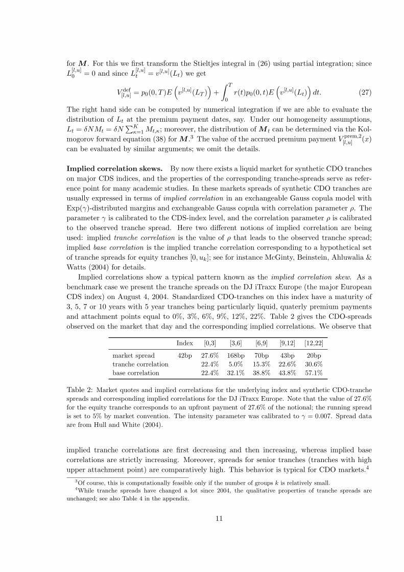
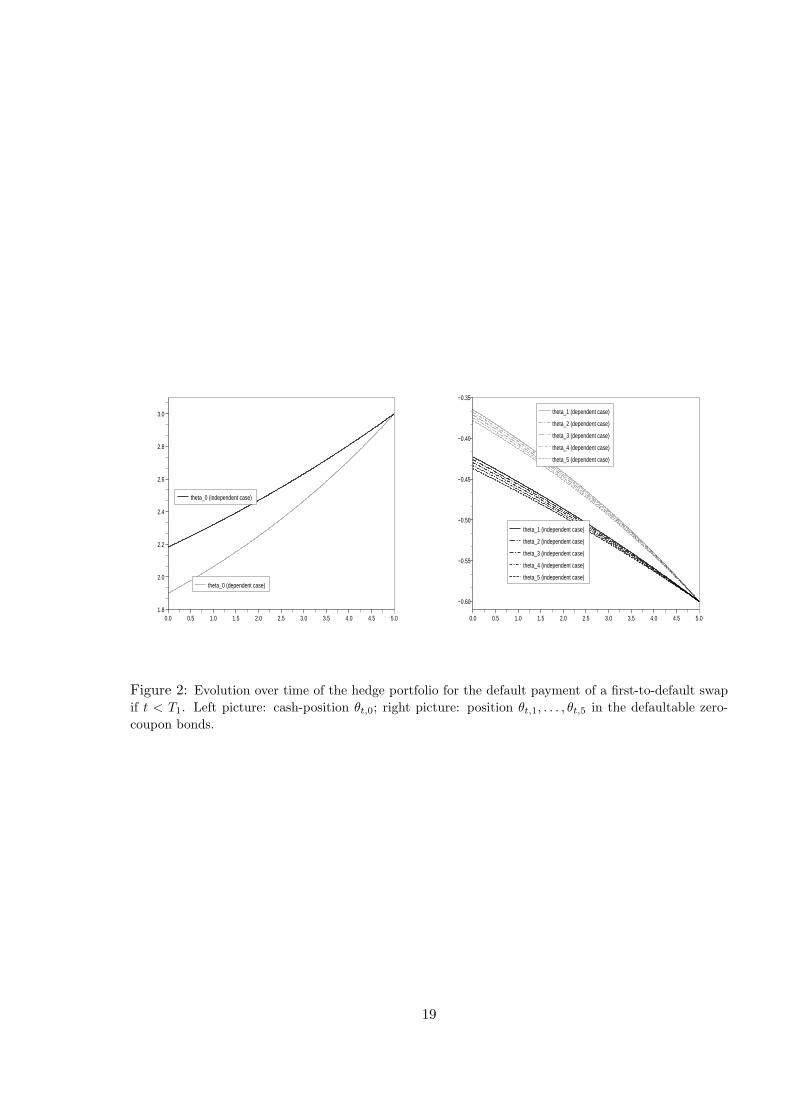
Implied correlations show a typical pattern known as the implied correlation skew. As abenchmark case we present the tranche spreads on the DJ iTraxx Europe (the major EuropeanCDS index) on August 4, 2004. Standardized CDO-tranches on this index have a maturity of3, 5, 7 or 10 years with 5 year tranches being particularly liquid, quaterly premium paymentsand attachment points equal to 0%, 3%, 6%, 9%, 12%, 22%. Table 2 gives the CDO-spreadsobserved on the market that day and the corresponding implied correlations. We observe that
Index [0,3] [3,6] [6,9] [9,12] [12,22]
market spread 42bp 27.6% 168bp 70bp 43bp 20bptranche correlation 22.4% 5.0% 15.3% 22.6% 30.6%base correlation 22.4% 32.1% 38.8% 43.8% 57.1%
Table 2: Market quotes and implied correlations for the underlying index and synthetic CDO-tranchespreads and corresponding implied correlations for the DJ iTraxx Europe. Note that the value of 27.6%for the equity tranche corresponds to an upfront payment of 27.6% of the notional; the running spreadis set to 5% by market convention. The intensity parameter was calibrated to γ = 0.007. Spread dataare from Hull and White (2004).
implied tranche correlations are first decreasing and then increasing, whereas implied basecorrelations are strictly increasing. Moreover, spreads for senior tranches (tranches with highupper attachment point) are comparatively high. This behavior is typical for CDO markets.4
3Of course, this is computationally feasible only if the number of groups k is relatively small.4While tranche spreads have changed a lot since 2004, the qualitative properties of tranche spreads are
unchanged; see also Table 4 in the appendix.
11

Explaining Correlation Skews Implied correlation skews reflect deficiencies of the ex-changeable Gauss copula model. In particular, the high implied correlations for the seniortranches show that market participants expect large clusters of defaults to occur more fre-quently than is consistent with a Gauss copula model. Most attempts to explain correlationskews start from this observation. For instance Hull & White (2004), Kalemanova, Schmid &Werner (2005), Guegan & Houdain (2005) or Elouerkhaoui (2006) consider models based onalternative copulas leading to more frequently occurring default clusters. Graziano & Rogers(2006) use a model with conditionally independent defaults driven by a Markov-chain; jumpsof the chain may moreover cause simultaneous defaults of several names.
We show next that is possible to generate correlation skews in the convex counterpartyrisk model (10) respectively (23). The basic idea is simple: by increasing λ2 we can generateoccasional large clusters of defaults without affecting the left tail of the distribution of Lt toomuch; in this way we can reproduce the high spread of the CDO tranches in a way which isconsistent with the observed spread of the equity tranche. To confirm this intuition we considerthe market data introduced in Table 2. In Table 3 we give the CDO spreads if the convexityparameter λ2 is varied; λ0 and λ1 were calibrated to the index level and the observed marketquote of the equity tranche. The results show that for appropriate values of λ2 the model canreproduce the qualitative behavior of the observed tranche spreads in a very satisfactory way.This observation is interesting as it provides an explanation of correlation skews of CDOs interms of the dynamics of the default indicator process.5 Similarly as in Andersen & Sidenius(2004), the model fit can be improved further by considering a state-dependent loss given defaultof the form δt = δ0 + δ1Mt for δ0 and δ1 > 0; see again Table 3 for details.
tranches [0,3] [3,6] [6,9] [9,12] [12,22]
market spreads 27.6% 168.0bp 70.0bp 43.0bp 20.0bp
model spreads∑
abs. err.
λ2 = 0 27.60% 223.1bp 114.5bp 61.1bp 16.9bp 120.8bpλ2 = 5 27.60% 194.2bp 95.7bp 54.9bp 23.3bp 67.1bpλ2 = 8 27.60% 172.1bp 80.0bp 46.7bp 23.7bp 21.5bpλ2 = 8.54 27.60% 168.0bp 77.1bp 45.1bp 23.5bp 12.7bpλ2 = 10 27.60% 156.9bp 69.4bp 40.7bp 22.7bp 16.7bpstate-dependent LGDδ0 = 0.5; δ1 = 7.5
27.60% 168.0bp 71.2bp 39.3bp 19.6bp 5.3bp
Table 3: CDO-spreads in the convex counterparty risk model (23) for varying λ2. λ0 and λ1 werecalibrated to the index level of 42bp and the market quote for the equity tranche, assuming δ = 0.6.For λ2 ∈ [8, 10] the qualitative properties of the model-generated CDO-spreads resemble closely thebehaviour of the market spreads; with state-dependent LGD the fit is almost perfect.
Implied correlations for CDO tranches on the iTraxx Europe have changed substantiallysince August 2004. More importantly, the analysis presented in Table 3 presents only a “snap-shot” of the CDO market at a single day. For these reasons we recalibrated the convex coun-terparty risk model 23 to 6 months of observed 5-year tranche spreads on the iTraxx Europe inthe period 23.9.2005–03.03.2006. In order to assess the issue of parameter-stability over time
5Qualitatively similar results were recently obtained in the related paper Herbertsson (2007).
12
we compared two different calibration approaches: first we did a full calibration where at agiven day λ0, λ1andλ2 were calibrated to the index level and the tranche spread of equity andjunior mezzanine tranche observed at that day; second, we did a partial calibration where at agiven day λ0 was calibrated to the index level observed at that day whereas for λ1 and λ2 weused the values obtained by full calibration on Sept, 23 2005 (the first day of the sample). Themotivation for this distinction is as follows: λ0 is a level parameter which is mainly influencedby the randomly fluctuating index spread so that one expects a lot of variability in this param-eter; λ1 and λ2 on the other hand are structure parameters which should be reasonably stableover time The results are contained in Table 4 in the appendix. A comparison of the tranchespreads obtained via full and partial calibration shows that partial calibration performs quitegood, indicating that the model does indeed give a reasonable description of the dynamics ofCDO markets.
4 Hedging Credit Derivatives
In this section we study the hedging of credit derivatives under Assumption 3.1. In particular,we give conditions ensuring that every HT -measurable claim can be replicated by dynamictrading in a portfolio of defaultable zero-coupon bonds and cash. Not surprisingly, it turnsout that our results depend strongly on the dynamic structure of the model, in particularon the choice of (Ht) as underlying filtration. This highlights a point made already in theintroduction: starting directly with assumptions on the joint distribution of τ1, . . . , τm andneglecting the dynamic aspects of the model - as it is done in most of the literature on factorcopula models - might be bad modelling practice. The hedging of credit risky securities is alsostudied in (Bielecki, Jeanblanc & Rutkowski 2004) and (Elouerkhaoui 2006), among others.
The hedging problem. We use the setup introduced in Assumption 3.1. The set of hedginginstruments consists of defaultable zero-coupon bonds issued by the m firms in the portfolio;for simplicity the bonds are assumed to have a zero recovery rate and fixed common maturityT . Recall that the price of the bond issued by firm j is vj(t,Yt) := p0(t, T )E(t,Yt)
((1− YT,j)
).
In the sequel we will work with discounted quantities using the default-free zero coupon bondp0(·, T ) as numeraire; the discounted price of the bond issued by firm j is then
vj(t,Yt) = E(t,Yt)
((1− YT,j)
). (28)
We are aware that this choice of hedging instruments is not in line with market practice -most practitioners regard single-name CDSs as natural hedging instruments for portfolio creditderivatives - but it is a useful first step. In principle, our arguments apply also to the prob-lem of hedging with CDSs. However, the gain process of these instruments takes on a quitecumbersome form, thus complicating the analysis considerably6.
We consider the problem of hedging a claim with maturity T , HT -measurable payoff H
and discounted price process Ht = E(H | Ht); since Y is Markov, in most cases of interest Ht
is in fact of the form vH(t,Yt) for some function vH : [0, T ] × SY → R. We are looking fora selffinancing portfolio strategy θH = (θH
t,0, . . . , θHt,m)0≤t≤T in the savings account and in the
defaultable zero-coupon bonds pj(·, T ), 1 ≤ j ≤ m, that replicates the claim H. By standard
6 The hedging with CDSs and CDS-indices is discussed in Frey & Backhaus (2007).
13

results on numeraire-invariance, this is equivalent to finding a representation of the martingaleH of the form
Ht = H0 +m∑
j=1
∫ t
0θHs,j dpj(s, T ) , 0 ≤ t ≤ T . (29)
We will approach this problem in two steps. First, we derive a martingale representationof H in terms of the compensated default indicator processes Nt,i := Yt,i −
∫ t∧τi
0 λi(s,Ys)ds,1 ≤ i ≤ m; in Step 2 we use this representation to give conditions for the existence of amartingale representation of H in terms of the discounted bond price processes pj(·, T ).
Step 1. Since there are no joint defaults in our model, the mark space of the marked pointprocess (Tn, ξn)1≤n≤m, is given by the set 1, . . . ,m. By standard results from stochasticcalculus - see for instance Jacod (1975) - every (Ht)-martingale can therefore be representedas stochastic integral with respect to the m martingales Nt,i, . . . , Nt,m, i.e. there are predicableprocesses φH
t,1, . . . , φHt,m such that
Ht = H0 +m∑
i=1
∫ t
0φH
s,idNs,i. (30)
The process φH is in fact easily determined: denote by At := 1 ≤ i ≤ m : Yt,i = 0 the set ofsurviving firms at time t. Since ∆Ht =
∑mi=1 φ
Ht,i∆Yt,i we get that
φHt,i0 =
m−1∑n=0
1]]Tn Tn+1]](t)1ATn(i0)
(E
(HT | HTn , Tn+1 = t, ξn+1 = i0
)− Ht
); (31)
if Ht = vH(t,Yt), (31) reduces to φHt,i0
= 1At(i0)(vH(t,Yi0
t ) − vH(t,Yt)). Note that φH is by
definition left-continuous.
Step 2. In analogy with (30), there are predictable vector-valued processes φj such that
pj(t, T ) = pj(0, T ) +m∑
i=1
∫ t
0φj
s,idNs,i, 1 ≤ j ≤ m. (32)
Hence the desired representation (29) can be written in the form
Ht = H0 +m∑
j=1
∫ t
0θHs,j d
( m∑i=1
∫ s
0φj
u,i dNu,i
)= H0 +
m∑i=1
∫ t
0
( m∑j=1
θHs,jφ
js,i
)dNs,i . (33)
Comparing (30) and (33), we obtain the following equations for the random variables θHt,j ,
j ∈ At, ∑j∈At
φjt,i θ
Ht,j = φH
t,i, i ∈ At , 0 ≤ t ≤ T ; (34)
for j /∈ At we let θHt,j = 0. Note that (34) is a linear system of |At| equations for |At| unknowns
with coefficient matrix Φt :=(φj
t,i
)i,j∈At
. Summing up, we therefore have
14
Proposition 4.1. Suppose that almost surely the matrix Φt has full rank for all t ∈ [0, T ].Then every HT -measurable claim can be replicated by dynamic trading in the savings accountand the defaultable zero-coupon bonds pj(·, T ), 1 ≤ j ≤ m. The trading strategy (θH
t,1, . . . , θHt,m)
is given as solution to the linear system (34) with coefficients φjt,i determined in (32) and right
hand side φHt,i determined in (30); θH
0 is determined by the selffinancing-condition.
Comments. 1. The system (34) can be simplified in the homogeneous-group case. In thatcase φj
t,i = ηκ(j)t,κ(i) and φH
t,i = ηHκ(i) for stochastic processes ηκ
t,ν , ηHt,ν , 1 ≤ ν, κ ≤ k. Hence also
θHt,j = ψH
t,κ(j) and the stochastic processes ψHt,κ, 1 ≤ κ ≤ k are determined by the following
system of k equations:
k∑κ=1
(mκ −Mt,κ)ηκt,νψ
Ht,κ = ηH
t,ν , 1 ≤ ν ≤ k. (35)
2. The same argument applies to other hedging instruments such as single-name CDSs; theonly thing that changes is the form of the integrands in the martingale representation of thecorresponding discounted gains-from-trade process with respect to Nt,1, . . . , Nt,m.3. The assumption that asset price processes are (Ht)-adapted is crucial for our analysis;without this assumption the martingale representations (30) and (32) break down. This as-sumption is not as innocent as it may seem: it implies that prices or spreads evolve determin-istically between defaults and react in a predictable way to default events in the portfolio. Inmarket-language, in our model there is event risk but between default times there is no spread-or market risk. This is admittedly unrealistic. However, the extension of the present hedgingframework to models with spread risk is a major undertaking and is therefore deferred to futurework.7.
The full-rank condition on Φt. For a given model and a given set of hedging instrumentsthe full rank condition is straightforward to verify. In the case of zero-recovery zero couponbonds as hedging instruments we can expect the full-rank condition to hold if the interactionbetween defaults is not too strong or if the time-to maturity is not too large, as we now show.By a similar reasoning as in (31), we obtain for i, j ∈ At
φjt,i = vj(t,Yi
t)− vj(t,Yt) . (36)
Note that for j ∈ At the element φjt,j = −vj(t,Yt) corresponds to the change in the value of
the bond due to default of the issuing firm j, whereas the off-diagonal elements φjt,i, i 6= j,
reflect the change in the value of the bond caused by the impact of the default of firm i on theconditional survival probability of the issuer j. In particular, with independent defaults φj
t,i = 0for i 6= j and φj
t,j < 0 for all j ∈ At. Hence Φt is a diagonal matrix with non-vanishing diagonalelements, and the full-rank condition is obviously satisfied. Now recall the following simpleresult from linear algebra: a generic matrix (aij)1≤i,j≤n is non-singular if it has a dominantdiagonal, i.e. if |aii| >
∑i6=j |aij | for all i ∈ 1, . . . , n. Since with independent defaults Φt is
diagonal, we expect that Φt has a dominant diagonal and therefore full rank, if the interaction7For hedging results in models with spread- and default risk we refer the reader to Frey & Backhaus (2007).
15

between default intensities is not to strong. A similar qualitative statement applies in the caseof a small time to maturity: Since vj(T,y) = p0(0, T )(1− yj), we get that
ΦT = diag(−p0(0, T ), . . . ,−p0(0, T )
).
Hence Φt has a dominant diagonal for t close to T (note that v is continuous in t).
Example 4.2 (Hedging of a survival claim and a first-to-default swap). We considera portfolio of m = 5 firms with intensity function λi(t,Yt) = λ0,i + λ1
(M(Yt)m ∧ 0.37
). Model
parameters are calibrated to the spread data of Example 3.2; for simplicity we take r(t) ≡ 0.Throughout we use zero-coupon bonds with zero recovery rate and a maturity of T = 5 yearsas hedging instruments.
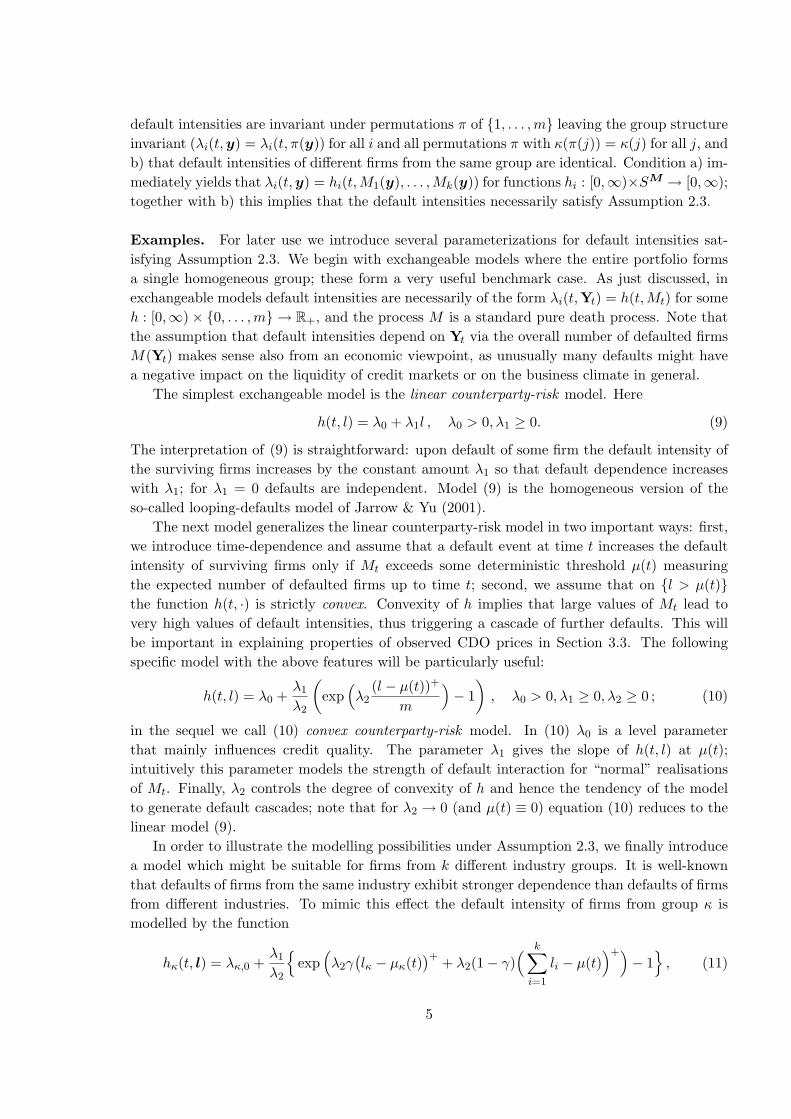
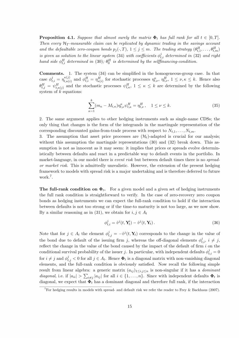
We start with the replication of a zero-coupon bond issued by Firm 1 with a maturity ofT0 = 0.5. With independent defaults (λ1 = 0), the hedge portfolio is constant and given byθt,1 ≡ p1(0, T0)/p1(0, T ); the cash position and the position in the bonds issued by Firm 2–5 (the firms not underlying the transaction) are identically zero. For λ1 > 0 the situationchanges. In that case the default of, say, Firm 2 leads to an increase in the default intensityof Firm 1, reducing the value of zero coupon bonds issued by Firm 1. This effect becomesstronger with increasing time to maturity, so that |∆p1(τ2, T0)| < |∆p1(τ2, T )|. To make upfor the ensuing loss, the hedger has to take a short position in p2(·, T ). A similar argumentapplies to Firm 3, 4 and 5. Numerical values for the position in the risky zero-coupon bonds areplotted in Figure 1. The example shows that in the presence of default contagion the replicatingportfolio of a single-name credit derivative may contain defaultable securities issued by firmsnot directly underlying the transaction.
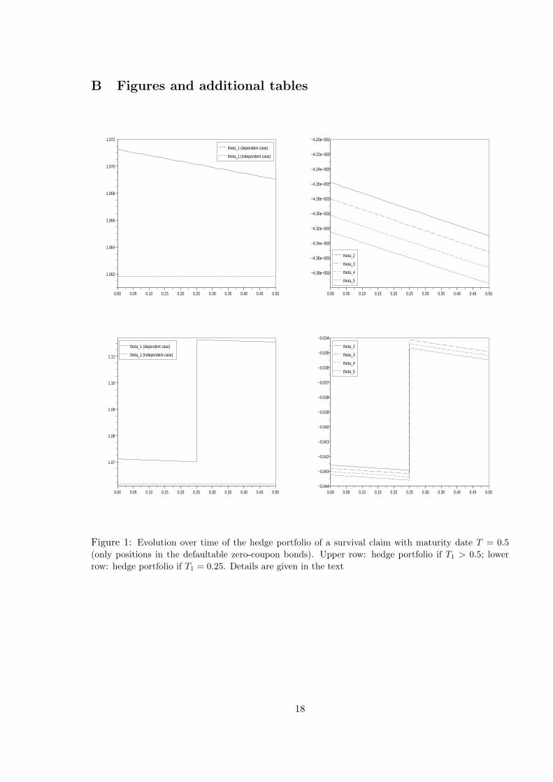
Next we consider the default payment of a first-to-default swap. The corresponding hedgingstrategy is illustrated numerically in Figure 2. The portfolio consists of a short position in allthe defaultable bonds underlying the transaction; in this way the portfolio produces a gain atT1 which compensates the default payment. For λ1 > 0 the absolute size of this short-positionis reduced compared to the case of independent defaults. Intuitively, this is due to the fact thatwith default contagion ∆pi(T1, T ) < 0 also for the surviving firms i ∈ AT1 . Since θT1,i < 0 thisleads to a an additional increase in the value of the hedge portfolio at T1 which contributes tofinancing the payoff of the claim.
A Numerical tools for the Markov model
We present standard approaches for the numerical treatment of (time-inhomogeneous) finite-state markov chains; see for instance Norris (1997) for the theoretical foundations.
A.1 Monte Carlo
For the convenience of the reader we recall the standard algorithm for generating trajectoriesof Y (or equivalently realisations of the sequence (Tn, ξn)1≤n≤m).
Algorithm A.1. 1. Generate independent random variables Z1, . . . , Zm, U1, . . . , Um withZi ∼ Exp(1), Ui ∼ U(0, 1). Put T0 = 0, y(0) = 0, n = 1, and define λ(1)
t :=∑m
i=1(1 −y
(0)i )λi(t,y(0)).
16

2. Given Tn−1, y(n−1), (λ(n)t )t≥Tn−1 , let Tn := inf
t ≥ Tn−1 :
∫ tTn−1
λ(n)s ds ≥ Zn
and let
ξn := i if∑i−1
j=1(1− y(n−1)j )λj(Tn,y
(n−1)) ≤ λ(n)TnUn <
∑ij=1(1− y
(n−1)j )λj(Tn,y
(n−1)).
3. If n = m stop. Else, set y(n) :=(y
(n−1)1 , . . . , 1 − y
(n−1)ξn
, . . . , y(n−1)m
), define for t ≥ Tn
λ(n+1)t :=
∑mi=1(1− y
(n)i )λi(t,y(n)), replace n with n+ 1 and continue with Step 2.
A.2 Kolmogorov equations
The backward equation is an ODE system for the function (t,y1) → p(t, s,y1,y2), 0 ≤ t ≤ s;s and y2 are considered as parameters. The equation has the form
∂
∂tp(t, s,y1,y2) +G[t]p(t, s,y1,y2) = 0 for 0 ≤ t < s, p(s, s,y1,y2) = 1y2(y1). (37)
The forward-equation is an ODE-System for the function (s,y2) → p(t, s,y1,y2), s ≥ t,which is governed by the adjoint operator G∗[s]. In its general form the forward equation reads∂∂sp(t, s,y1,y2) = G∗[s]p(t, s,y1,y2) with initial condition p(t, t,y1,y2) = 1y1(y2). This leadsto the following system of ODEs:
∂p(t, s,y1,y2)∂s
=∑
j : y1,j=1
λj(s,yj2)p(t, s,y1,y
j2) −
∑j : y2,j=0
λj(s,y2)p(t, s,y1,y2); (38)
for a formal proof see Appendix A.2 of Frey & Backhaus (2004). Note that the first term onthe right in (38) gives the instantaneous increase in the probability p(t, s,y1,y2) due to jumpsfrom neighboring states yj
2 into the state y2; the second term gives the instantaneous decreasedue to jumps from y2 to the neighboring states yj
2, 1 ≤ j ≤ m.Of course, it is also possible to derive the Kolmogorov equations for the transition proba-
bilities of M . The exact form of the ODE-system for the backward equation is obvious. Forthe forward equation we obtain the following ODE-system
∂pM (t, s, l1, l2)∂s
=k∑
κ=1
1l2κ>0(mκ − l2κ) + 1
)hκ
(s, l2 − eκ
)pM
(t, s, l1, l2 − eκ
)−
k∑κ=1
mκ − l2κhκ(s, l2)pM (t, s, l1, l2)
with initial condition pM (t, t, l1, l2) = 1l1(l2).
17
B Figures and additional tables
0.00 0.05 0.10 0.15 0.20 0.25 0.30 0.35 0.40 0.45 0.50
1.062
1.064
1.066
1.068
1.070
1.072
theta_1 (dependent case)
theta_1 (independent case)
0.00 0.05 0.10 0.15 0.20 0.25 0.30 0.35 0.40 0.45 0.50
−4.38e−002
−4.36e−002
−4.34e−002
−4.32e−002
−4.30e−002
−4.28e−002
−4.26e−002
−4.24e−002
−4.22e−002
−4.20e−002
theta_2
theta_3
theta_4
theta_5
0.00 0.05 0.10 0.15 0.20 0.25 0.30 0.35 0.40 0.45 0.50
1.07
1.08
1.09
1.10
1.11
theta_1 (dependent case)
theta_1 (independent case)
0.00 0.05 0.10 0.15 0.20 0.25 0.30 0.35 0.40 0.45 0.50−0.044
−0.043
−0.042
−0.041
−0.040
−0.039
−0.038
−0.037
−0.036
−0.035
−0.034
theta_2
theta_3
theta_4
theta_5
Figure 1: Evolution over time of the hedge portfolio of a survival claim with maturity date T = 0.5(only positions in the defaultable zero-coupon bonds). Upper row: hedge portfolio if T1 > 0.5; lowerrow: hedge portfolio if T1 = 0.25. Details are given in the text
18
0.0 0.5 1.0 1.5 2.0 2.5 3.0 3.5 4.0 4.5 5.01.8
2.0
2.2
2.4
2.6
2.8
3.0
theta_0 (dependent case)
theta_0 (independent case)
0.0 0.5 1.0 1.5 2.0 2.5 3.0 3.5 4.0 4.5 5.0
−0.60
−0.55
−0.50
−0.45
−0.40
−0.35
theta_1 (dependent case)
theta_2 (dependent case)
theta_3 (dependent case)
theta_4 (dependent case)
theta_5 (dependent case)
theta_1 (independent case)
theta_2 (independent case)
theta_3 (independent case)
theta_4 (independent case)
theta_5 (independent case)
Figure 2: Evolution over time of the hedge portfolio for the default payment of a first-to-default swapif t < T1. Left picture: cash-position θt,0; right picture: position θt,1, . . . , θt,5 in the defaultable zero-coupon bonds.
19
[0,3
]tr
anch
e[3
,6]tr
anch
e[6
,9]tr
anch
e[9
,12]
tran
che
[12,
22]tr
anch
e
Spre
adSp
read
Spre
adSp
read
Spre
adTr.
Cor
r.Tr.
Cor
r.Tr.
Cor
r.Tr.
Cor
r.Tr.
Cor
r.
Dat
e
Indexspread
market
full
partial
market
full
partial
market
full
partial
market
full
partial
market
full
partial
λ0
23.0
9.20
0539
3131
3110
310
310
336
2929
1617
179
1212
0.00
4668
15.7
15.7
15.7
2.2
2.2
2.2
10.4
9.1
9.1
14.6
14.8
14.8
23.4
26.2
26.2
30.0
9.20
0536
.328
2827
9292
9227
2526
1214
157
1011
0.00
4318
15.9
15.9
16.3
3.0
3.0
3.0
10.0
9.7
9.7
14.2
15.3
15.4
22.9
26.4
26.6
07.1
0.20
0537
.530
3029
9898
9728
2627
1314
166
1012
0.00
4481
14.9
14.9
16.3
2.8
2.8
2.7
9.6
9.3
9.5
14.1
14.8
15.2
21.2
25.6
26.6
04.1
1.20
0537
2929
2893
9394
2325
2612
1415
610
110.
0044
4514
.914
.916
.23.
03.
03.
09.
09.
49.
714
.114
.915
.421
.625
.926
.602
.12.
2005
3526
2626
7575
8522
2024
1112
136
1010
0.00
4218
15.9
15.9
16.6
2.0
2.0
3.8
9.9
9.4
10.3
14.7
15.2
15.9
22.3
26.8
27.0
06.0
1.20
0636
2626
2783
8389
2823
2413
1413
611
100.
0043
8816
.916
.915
.83.
33.
33.
711
.09.
910
.115
.415
.815
.622
.522
.826
.403
.02.
2006
3627
2727
7676
8826
1923
1111
135
99
0.00
4423
15.1
15.1
15.4
3.0
3.0
3.9
10.8
9.1
10.1
14.7
14.9
15.5
21.5
26.3
26.1
03.0
3.20
0635
.527
2726
6767
8522
1622
1210
125
89
0.00
4391
13.9
13.9
15.2
2.8
2.8
4.2
10.3
8.6
10.2
15.6
14.4
15.5
21.9
25.8
26.0
Tab
le4:
Cal
ibra
tion
ofth
em
odel
(23)
toiT
raxx
Eur
ope
inde
xan
dtr
anch
esp
read
sus
ing
full
and
part
ialc
alib
rati
on.
The
para
met
ers
used
for
part
ial
calib
rati
onar
eλ
1=
0.19
21an
dλ
2=
20.7
3.A
com
pari
son
ofth
etr
anch
esp
read
sob
tain
edvi
afu
llan
dpa
rtia
lcal
ibra
tion
show
sth
atpa
rtia
lcal
ibra
tion
perf
orm
squ
ite
good
;de
tails
are
give
nin
the
text
.
20

References
Andersen, L. & Sidenius, J. (2004), ‘Extensions to the Gaussian copula: Random recovery and randomfactor loadings’, Journal of Credit Risk 1, 29–70.
Avellaneda, M. & Wu, L. (2001), ‘Credit contagion: pricing cross country risk in the Brady bond market’,International Journal of Theoretical and Applied Finance 4, 921–939.
Bielecki, T., Jeanblanc, M. & Rutkowski, M. (2004), Hedging of defaultable claims, in ‘Paris-PrincetonLectures on Mathematical Finance’, Vol. 1847 of Springer Lecture Notes in Mathematics, Springer.
Bielecki, T. Vidozzi, A. & Vidozzi, L. (2006), ‘An efficient approach to valuation of credit basket productsand rating-triggered step-up bonds’, working paper, Illinois Institute of Technology.
Davis, M. & Lo, V. (2001), ‘Infectious defaults’, Quant. Finance 1, 382–387.
Duffie, D. & Garleanu, N. (2001), ‘Risk and valuation of collateralized debt obligations’, FinancialAnalyst’s Journal 57(1), 41–59.
Elouerkhaoui, Y. (2006), Etude des Problemes de Correlation et d’Incompletude dans les Marches deCredit, PhD thesis, Universite Paris IX Dauphine. in English.
Frey, R. (2003), ‘A mean-field model for interacting defaults and counterparty risk’, Bulletin of theInternational Statistical Institute.
Frey, R. & Backhaus, J. (2004), ‘Portfolio credit risk models with interacting default intensities: a Marko-vian approach’, Preprint, Universitat Leipzig. available from www.math.uni-leipzig.de/~frey.
Frey, R. & Backhaus, J. (2007), ‘Dynamic hedging of synthetic CDO-tranches with spread- andcontagion risk’, preprint, department of mathematics, Universitat Leipzig. available fromhttp://www.math.uni-leipzig.de/ frey/publications-frey.html.
Giesecke, K. & Weber, S. (2006), ‘Credit contagion and aggregate losses’, J. Econom. Dynam. Control30, 741–767.
Graziano, G. & Rogers, C. (2006), ‘A dynamic approach to the modelling of correlation credit derivativesusing Markov chains’, working paper, Statistical Laboratory, University of Cambridge.
Guegan, D. & Houdain, J. (2005), ‘Collateralized debt obligations pricing and factor models: A newmethodology using normal inverse gaussian distributions’, working paper, ENS, Cachan.
Herbertsson, A. (2007), ‘Pricing synthetic CDO tranches in a model with default contagion using thematrix-analytic approach’, working paper, Goteborg University.
Horst, U. (2006), ‘Stochastic cascades, credit contagion and large portfolio losses’, Journal of EconomicBehavior and Organization . to appear.
Hull, J. & White, A. (2004), ‘Valuation of a CDO and a nth to default CDS without Monte Carlosimulation’, Journal of Derivatives 12, 8–23.
Jacod, J. (1975), ‘Multivariate point processes: predictable projection, Radon-Nikodym derivatives,representation of martingales’, Z. Wahrscheinlichkeitstheorie verw. Gebiete 31, 235–253.
Jarrow, R. & Yu, F. (2001), ‘Counterparty risk and the pricing of defaultable securities’, J. Finance56, 1765–1799.
Kalemanova, A., Schmid, B. & Werner, R. (2005), ‘The normal inverse gaussian distribution for syntheticCDO pricing’, working paper, Risklab Germany.
Lando, D. (1998), ‘Cox processes and credit risky securities’, Rev. Derivatives Res. 2, 99–120.
21

Laurent, J. & Gregory, J. (2005), ‘Basket default swaps, CDOs and factor copulas’, Journal of Risk7, 103–122.
Li, D. (2001), ‘On default correlation: a copula function approach’, J. of Fixed Income 9, 43–54.
McGinty, L., Beinstein, E., Ahluwalia, R. & Watts, M. (2004), ‘Introducing base correlation’, Preprint,JP Morgan.
McNeil, A., Frey, R. & Embrechts, P. (2005), Quantitative Risk Management: Concepts, Techniques andTools, Princeton University Press, Princeton, New Jersey.
Norris, J. (1997), Markov Chains, Cambridge University Press.
Schonbucher, P. (2004), ‘Information-driven default contagion’, Preprint, Department of Mathematics,ETH Zurich.
Yu, F. (2007), ‘Correlated defaults in intensity-based models’, Math. Finance 17, 155–173.
22