Price dispersion, information and learningaraujolu/Price Dispersion, Information and... · Price dispersion, information and learning$ Luis Araujoa,b, ... actual quantity of goods

ARTICLE IN PRESS

Journal of Monetary Economics 53 (2006) 1197–1223

0304-3932/$ -

doi:10.1016/j

$We wish

thank semin

Thanksgiving�CorrespoE-mail ad

www.elsevier.com/locate/jme

Price dispersion, information and learning$

Luis Araujoa,b, Andrei Shevchenkoa,�

aDepartment of Economics, Michigan State University, 101 Marshall Hall, East Lansing, MI 48824-1038, USAbFucape Business School, Brazil

Received 14 October 2004; received in revised form 5 April 2005; accepted 11 April 2005

Available online 8 May 2006

Abstract

We consider an economy where trade is decentralized and agents have incomplete information

with respect to the value of money. Agents’ learning evolves from private experiences and we explore

how the formation of prices interacts with learning. We show that multiple equilibria arise, and

equilibria with price dispersion entail more learning than equilibria with one price. Price dispersion

increases communication about private histories, which in turn increases the overall amount of

information in the economy. We also compare ex ante welfare under price dispersion and one price.

Our results show that, despite the existence of some meetings where no trade takes place, ex ante

welfare under price dispersion may be higher than under one price.

r 2006 Elsevier B.V. All rights reserved.

JEL classification: E40; D82; D83

Keywords: Search; Money; Price dispersion; Learning

1. Introduction

We use a random-matching model of money to study the interaction between learningand the real effects of monetary uncertainty in the short-run. It has become an agreementpoint in the literature that in order to get output fluctuations from monetary shocks onehas to assume some type of uncertainty and decentralized markets (see Lucas, 1996). The

see front matter r 2006 Elsevier B.V. All rights reserved.

.jmoneco.2005.04.007

to thank Gabriele Camera, Neil Wallace and Randall Wright for very helpful comments. We also

ar participants at Indiana, Michigan State University, Federal Reserve Bank of Cleveland,

Conference at Penn State University and the 2004 SED Meetings.

nding author. Tel.: +1517 353 5007; fax: +1 517 432 1068.

dress: [email protected] (A. Shevchenko).

www.elsevier.com/locate/jme

dx.doi.org/10.1016/j.jmoneco.2005.04.007

mailto:[email protected]

ARTICLE IN PRESSL. Araujo, A. Shevchenko / Journal of Monetary Economics 53 (2006) 1197–12231198

search-theoretic framework, although stylized, is very useful in studying this type ofquestion. It provides a deep theory of money as a medium of exchange and at the sametime it allows us to introduce an environment with imperfectly informed agents anddecentralized trade. The same frictions that generate an essential role for money makelearning very interesting but still tractable.Since Lucas (1972) there has been a significant number of papers developing models

consistent with the observed short-run and long-run relationship between changes in thesupply of money and fluctuations in output and prices. The underlying argument in thosepapers implicitly assumes that it takes time for agents to learn the true state of theeconomy. However, the informational structure of these models usually does not leavemuch space for learning. Moreover, it exogenously assumes a particular form of one-sidedasymmetric information where consumers are informed but producers are uninformedabout the actual value of money. Barro and King (1984) point out that the actualdistribution of information can be of crucial importance in the determination of the effectsof money on output.More recently, the original environment of Lucas (1972) has been enriched through the

use of more sophisticated informational structures. Examples are Jones and Manuelli(2001) and Katzman et al. (2003). Each one of these papers develops a model with pairwisetrade and one-sided asymmetric information. As an important novelty, they allow for aseparation between informed–uninformed status and consumer–producer status. Katzmanet al. (2003) assume an exogenous informational asymmetry: some agents observemonetary shocks as they occur and others observe them only with a one-period lag. Jonesand Manuelli (2001) allow for costly information acquisition and as a result anendogenously chosen information structure arises.We depart from the previous literature by considering an economy with two-sided

asymmetric information. More precisely, instead of assuming informational asymmetryfrom the beginning, we introduce homogeneous agents with an access to the sameinformation technology. Agents learn from their private experiences in the market and weassume that each agent receives the same amount of information. A result of this learningprocess is the emergence of two-sided informational asymmetries and correlation of privateexperiences. These features are not present in models with one-sided asymmetricinformation and they have important short-run implications in the economy.In this paper, we explore the interaction between learning and the formation of prices.

We obtain that, in addition to equilibria with one price, equilibria with price dispersion canarise. The intuition for this result runs as follows. In a decentralized environment, distinctprivate experiences lead to distinct beliefs about the state of the economy. This implies thatan agent’s behavior in a trade meeting can be contingent on his history. Moreover, sinceprivate histories are correlated, buyers with a belief that money has a high value have moreincentives to ask for a low price since they believe that there is a higher probability thatsuch an offer is going to be accepted. As a result, prices convey information about the stateof the economy.In what follows, we provide a region of parameters where both one price and price

dispersion arises and we show that, despite the existence of trade meetings where no tradetakes place, price dispersion equilibrium may entail higher production and higher ex antewelfare than the one-price equilibrium. Positive aspects of price dispersion have not beenemphasized in the literature. Usually, price dispersion is Pareto dominated by a single-price equilibrium. This has been suggested either explicitly by Stigler (1961) (see also Rob,

ARTICLE IN PRESSL. Araujo, A. Shevchenko / Journal of Monetary Economics 53 (2006) 1197–1223 1199

1985) or implicitly (see Burdett and Judd, 1983) by equilibrium price dispersion theory. Inthis theory, price dispersion arises as a result of costly or noisy search and differentialinformation. The essence of the theory is that a distribution of prices for a homogeneousgood causes confusion about the true value of money: ‘‘Price dispersion is amanifestation—and, indeed, it is the measure—of ignorance in the market’’ (Stigler,1961, p. 214). In our environment exactly the opposite is true: price dispersion providesagents with additional information that helps them learn the true state of the economy.

The rest of the paper proceeds as follows. The next section describes the model,strategies and the equilibrium concept. The section after that characterizes an equilibriumwhere prices reveal no information. In Section 4, we describe an equilibrium where pricesconvey information about the actual value of money. Section 5 characterizes the parameterregion where both the equilibrium with one price and with price dispersion exist. In Section6, we derive the welfare results. Section 7 discusses the robustness of the model and Section8 concludes. Proofs are in the Appendix.

2. The model

We adopt a version of the environment similar to the one studied by Trejos and Wright(1995), Shi (1995) and Wallace (1997). Consider an economy with a continuum of agentsand K divisible and perishable goods. Time is discrete and indexed by t. Agents can be of K

distinct types. A type i agent derives utility from the consumption of good i and is able toproduce good i þ 1 (modulo K) and there is a uniform distribution of agents across types.Utility in every period is given by uðxÞ � y, where x is the amount consumed and y is theamount produced. The function u is defined on ½0;1Þ and uð:Þ is increasing, twicedifferentiable, uð0Þ ¼ 0, u00o0 and u0ð0Þ ¼ 1. Agents maximize expected discounted utilitywith a discount factor b 2 ð0; 1Þ. In the economy there is also a storable, indivisible andintrinsically useless object, which we denote as fiat money. We assume that an agent canhold at most one unit of money at a time.

A key feature of the environment is that trade is decentralized and agents face frictionsin the exchange process. We formalize this idea by assuming that there are K distinctsectors, each one specialized in the exchange of one good. Agents can identify the sectorsbut inside each sector they are anonymously and pairwise matched under a uniformrandom matching technology. Each agent faces one meeting per period. Moreover,meetings are independent across agents and independent over time. Therefore, if an agentwants money he goes to the sector which trades his endowment and searches for an agentwith money. If he has money he goes to the sector that trades the good he likes andsearches for an agent with the good. Since there is an upper bound on money holdings, atransaction can happen only when an agent with money (buyer) meets an agent withoutmoney (seller). We denote meetings of this sort as trade meetings. We assume a very simpleexchange protocol in a trade meeting, namely, take it or leave it offers by the buyer. Inparticular, we assume that an offer consists of a demand for an amount of production. Ifthe offer is accepted, trade happens. Otherwise, there is no trade.

At date 0, money is randomly distributed in the economy. We assume that all features ofthe environment are common knowledge across agents with the exception of the amount ofmoney in the economy. In particular, the fraction of agents that receive money is equal tom, where m can be either mH or mL, with mH4mL. If mH (mLÞ is realized, we say that the


economy is in the high (low) state. Before money is distributed agents have a commonprior y, indicating the probability that m ¼ mH .The economy is divided in a short-run period and a long-run period. In the short-run

agents face incomplete information with respect to the value of m. In the long-run theactual state of the economy (mH or mL) is revealed to all agents. Wallace (1997) assumesthat the short-run lasts for one period. However, he states that: ‘‘. . .the natural assumptionis that it (the quantity of money) is never revealed.’’ He continues: ‘‘I see two difficulties inworking with that specification or even one that lengthens the lag beyond one period. First,priors get revised in accord with experiences. Since experience is diverse, one would have tokeep track of groups that are diverse in terms of their posteriors over the realized change inthe amount of money. Second, the bargaining would then occur between two people whodo not know each other’s posteriors’’ ((1997), pp. 1304 and 1305).1

In what follows we add one more period to the short-run. As Wallace anticipates, bydoing this we need to keep track of groups of agents with distinct posteriors and we alsoneed to deal with a bargaining process where agents in a match do not know with certaintyeach other’s posteriors. The benefit of this modification is that it delivers a natural way inwhich prices and learning interact in decentralized economies.Finally, note that in random matching models with an upper bound on money holdings,

changes in the amount of money have two different margins, extensive and intensive. Theextensive margin is related to the rate at which trade meetings take place, which dependson the distribution of money in the economy. The intensive margin corresponds to theactual quantity of goods produced in trade meetings. Our primary objective is to analyzethe relation between learning and the formation of prices. Hence, in what follows werestrict attention to the intensive margin effects by assuming that mH þmL ¼ 1. Thisassumption is meant as a way to control for the extensive margin effects since it impliesthat the number of trade meetings is independent of the state of the economy. Itsrobustness is discussed in more detail in Section 7.

2.1. Benchmark

We consider first a simple version of the model where the short-run has only one period(date 1). The purpose is to provide a framework that can be more easily compared withprevious models. First, consider the economy at date t (t41), after the state (high or low)be revealed to all agents. Let V 0ðmÞ be the value function of an agent without money andlet V1ðmÞ be the corresponding value function for an agent with money, when the amountof money is m. We have

V 0ðmÞ ¼ mð�yþ bV1ðmÞÞ þ ð1�mÞbV 0ðmÞ,

V 1ðmÞ ¼ mbV1ðmÞ þ ð1�mÞðuðyÞ þ bV 0ðmÞÞ.

For example, if an agent has money he goes to the sector that trades the good he likes. Inthis sector, there is a probability m that he meets another agent with money and no tradehappens. There is also a probability ð1�mÞ that he meets an agent without money. In thiscase they trade, the agent obtains utility uðyÞ, where y is the amount produced by the seller,

1Among others, Wolinsky (1990) and Araujo and Camargo (2005) analyze a decentralized economy where

information is never revealed. However, both papers assume exogenous prices.


and moves to the next period without money. A similar reasoning holds for an agentwithout money.

At each date t41, a seller is going to accept an offer from the buyer as long as the valueof becoming an agent with money tomorrow minus the production cost today is greaterthan the value of going to the next period without money, i.e., as long as

bV 1ðmÞ � yXbV 0ðmÞ.

Let Dðy;mÞ ¼ V1ðmÞ � V 0ðmÞ. Note that

Dðy;mÞ ¼ ð1�mÞuðyÞ þmy.

The assumption that buyers make a take it or leave it offer implies

y ¼ bDðy;mÞ. (1)

Condition ð1Þ can be rewritten as

y ¼bð1�mÞuðyÞ

1� bm.

It is easy to see that, as the amount of money in the economy increases, the value of y

decreases. The intuition is simple. If a seller anticipates that a large fraction of agents isholding money, the probability of meeting an agent that has the good he likes goes down.Therefore, he is going to produce less today in exchange for money.

Now, consider the economy at date 1. Let y1ð1Þ (y1ð0Þ) indicates the belief that theeconomy is in the high state for an agent starting with (without) money. Bayesian updatingimplies

y1ð1Þ ¼mHy

mHyþmLð1� yÞ

and

y1ð0Þ ¼ð1�mH Þy

ð1�mH Þyþ ð1�mLÞð1� yÞ.

Agents meet in pairs under a uniform random matching technology. These meetings giveadditional information about the state of the economy and, based on this information,buyers make take it or leave it offers to sellers.

In a trade meeting in the short-run, the information of the buyer can be summarized bythe pair ð1; 0Þ, where 1 indicates that he had money and 0 indicates that he met an agentwithout money. Analogously, the information of the seller corresponds to the pair ð0; 1Þ.Since meetings are random and the probability of meeting an agent with money is the sameprobability of starting with money in the economy, we obtain that both the buyer and theseller form the same posterior with respect to the state of the economy. This posterior isequal to

y2ð1Þ ¼mH ð1�mH Þy

mHð1�mHÞyþmLð1�mLÞð1� yÞ,

where y2ð1Þ indicates a private history with a length 2 and a cardinality equal to 1. Moregenerally, the belief after a history of length i and cardinality j will be denoted as yiðjÞ. LetV 2

tðyÞ be the value function at the beginning of date 2, i.e., before the state of the economybe revealed to all agents, for an agent with t units of money (t ¼ 0; 1) and a posterior y. We


obtain

V 20ðy2ð1ÞÞ ¼ y2ð1ÞV0ðmH Þ þ ð1� y2ð1ÞÞV 0ðmLÞ

and

V 21ðy2ð1ÞÞ ¼ y2ð1ÞV1ðmH Þ þ ð1� y2ð1ÞÞV 1ðmLÞ.

In the short-run, a take it or leave it offer y by the buyer implies

y ¼ b½V21ðy2ð1ÞÞ � V 2

0ðy2ð1ÞÞ� ¼ y2ð1ÞyH þ ð1� y2ð1ÞÞyL,

where yH ðyLÞ is the amount produced in the high (low) state under complete information,with yL4yH .We observe that, in the short-run, despite the actual realization of the state, the price

level ð1=yÞ does not change. In the long-run prices reflect the actual state. If the state is mH ,the price is equal to 1=yH . If it is mL, price is equal to 1=yL. Since mH4mL, we have thatprices in the high state are higher than in the low state. The result that prices in the short-run are independent of the state of the economy is a consequence of the informationalstructure. Since all agents in trade meetings in the short-run have a common belief, it isnatural that only one price arises.2

2.2. Strategies and equilibrium concept

We now consider an economy where the short-run has two periods (date 0 and date 1).Assume that agents start at date 0 with a common prior y. Over time beliefs are updatedaccording to private experiences and this updating process goes on until date 2, when theinformation about the state of the economy is then revealed. An agent’s strategy specifiesan action at every information set. At any date t, where tX2, since the state of the economyis revealed to all agents in the economy, information sets are fHg and fLg, indicatingwhether the high or the low state is realized. At dates 0 and 1, an agent’s information setcorresponds to his private history. A private history is a complete record of the agent’sinitial money holdings, the money holdings of all his partners and the outcome of all hispast meetings.At dates tX2 the buyer’s behavior is given by

stB : fH;Lg ! Rþ for all tX2

and the seller’s behavior is given by

stS : fH;Lg � Rþ ! fA;Rg for all tX2,

where A indicates that the offer is accepted and R indicates that it is rejected. At date 0,since buyers and sellers face private histories which are equivalent from an informationalpoint of view (see previous section), a buyer’s behavior is given by

s0B 2 Rþ

2Despite some differences in the environment, these results are very similar to the ones obtained by Wallace

(1997). The main objective in Wallace is to show how a random matching model can generate short-run effects of

changes in the quantity of money which are mainly real, and long-run effects which are mainly nominal.


and a seller’s behavior is given by

s0S : Rþ ! fA;Rg.

Now consider the economy at date 1. At this date, an agent’s private history is only therecord of his money holdings and the money holdings of his partner at dates 0 and 1.Clearly, the price observed at date 0 does not add any new information. As a result, the setof private histories of a seller at date 1 are

OS3ð1Þ ¼ ð0; 0; 1Þ and OS

3ð2Þ ¼ ð1; 0; 1Þ.

Similarly, the buyer’s private histories at date 1 are

OB3 ð1Þ ¼ ð0; 1; 0Þ and OB

3 ð2Þ ¼ ð1; 1; 0Þ.

Hence, buyer’s behavior at date 1 is given by

s1B : fOB3 ð1Þ;O

B3 ð2Þg ! Rþ

and the seller’s behavior is

s1S : fOS3ð1Þ;O

S3ð2Þg � Rþ ! fA;Rg.

Consider the collection s ¼ fstB;s

tSg1t¼0 and a belief function for the seller at date 1,

m : Rþ ! ½0; 1�, where mðyÞ indicates the probability that the buyer has a history OB3 ð1Þ

when the seller observes a demand equal to y. We restrict attention to symmetric strategies,i.e., agents choose the same action if they face the same private history. A perfect Bayesianequilibrium is a pair fs;mg such that an agent’s behavior at any information set is optimalgiven the behavior specified at all other information sets, and beliefs are calculated fromBayes rule whenever possible.

3. An equilibrium where prices are non-informative

We describe the conditions under which in every period only one price emerges in theshort-run and all sellers accept this price, irrespective of the state of the economy. We firstinformally discuss our main result. Proposition 1 provides a formal proof.

First, note that in trade meetings from date 2 onwards, the amount of output is equal toyH (yL) depending on the state of the economy being high (low). This fact allows us towork backwards and describe the agent’s optimal decision at dates 0 and 1.

3.1. Date 1

Consider a trade meeting at date 1. In this meeting, depending on his belief about thestate of the economy, a buyer makes a take it or leave it offer to the seller. The seller, alsoas a function of his belief, accepts or rejects the offer. We first describe the possibleposteriors of buyers and sellers.

Consider the problem faced by a seller in a trade meeting at date 1. Moreover, assumethat his private history is OS

3ð1Þ. This history leads to a posterior

y3ð1Þ ¼mH ð1�mH Þ

2y

mHð1�mHÞ2yþmLð1�mLÞ

2ð1� yÞ

.


Analogously, a history OS3ð2Þ leads to a posterior

y3ð2Þ ¼m2

H ð1�mH Þym2

H ð1�mH Þyþm2Lð1�mLÞð1� yÞ

.

Now assume that there is an equilibrium at date 1 where only one price is asked in allmeetings and all agents accept this price. This implies that, on the equilibrium path, when abuyer makes a take it or leave it offer to a seller, this offer does not modify the seller’sinformation set and, as a consequence, does not affect the seller’s posterior. Consider, first,a seller with a history OS

3ð1Þ. If all buyers ask for y, a seller accepts the offer as long as

ypb½V21ðy3ð1ÞÞ � V2

0ðy3ð1ÞÞ� � yl ¼ y3ð1ÞyH þ ð1� y3ð1ÞÞyL.

Alternatively, if all buyers ask for y and the seller has a history OS3ð2Þ, he accepts the offer

as long as

ypb½V21ðy3ð2ÞÞ � V2

0ðy3ð2ÞÞ� � yh ¼ y3ð2ÞyH þ ð1� y3ð2ÞÞyL.

Note that, since y3ð2Þ4y3ð1Þ, we have

yhoyl .

Therefore, if we want all buyers to make an offer which is accepted by all sellers, theyshould ask for yh. The intuition for this result is simple. The seller’s expected gain fromaccepting an offer is decreasing in his posterior about the state of the economy. As hebecomes more pessimistic (that is, as his expectation that the economy is in the high stateincreases), he is less willing to produce. Therefore, a buyer needs to ask for a productionamount which is accepted by the most pessimistic seller. In what follows we say that abuyer (seller) is optimistic if he has a history OB

3 ð1Þ (OS3ð1Þ) and pessimistic otherwise.

We also need to check the incentives of a buyer to demand a production consistent withall sellers accepting it. In principle, a buyer could ask for a higher production with the hopethat an optimistic seller would accept it. First, note that if there is a buyer willing to ask fora higher production it has to be an optimistic buyer. The reason is clear. The success of ademand for high production depends upon the buyer meeting an optimistic seller. Sinceoptimistic sellers are more frequent when the state of the economy is low, an agent with alow value of the posterior has more incentives to ask for a high demand.Therefore, we only need to check deviations from the one-price rule that come from an

optimistic buyer. If this buyer follows the proposed equilibrium and asks for yh, he obtainsuðyhÞ. In this case, he gives the money to the seller and moves to the next period withoutmoney. His overall payoff is equal to

uðyhÞ þ bV 20ðy3ð1ÞÞ.

However, he can deviate and ask for a higher amount. His expected payoff depends on thetype of the seller and on the belief that the seller attaches to the buyer’s possible types. Wecould assume, for example, that all sellers give equal weight to each of the buyer’s typeafter seeing any deviation from yh. These beliefs are consistent with the definition of aperfect Bayesian equilibrium.3 For now, we fix the seller’s belief and assume that the

3However, they may not pass the intuitive criterion of Cho and Kreps (1987), which imposes further constraints

on beliefs out of the equilibrium path. In the proof of Proposition 1, we analyze this issue in detail.


maximum demand of output consistent with partial acceptance (i.e., only optimistic sellersaccept the offer) is equal to y, where y4yh.

Define P00 as the probability that an optimistic buyer meets an optimistic seller.Formally, we have

P00 ¼ y3ð1Þð1�mH Þ þ ð1� y3ð1ÞÞð1�mLÞ.

After some algebraic manipulation we obtain that an optimistic buyer is not going todeviate from the proposed one-price equilibrium as long as

uðyhÞXP00uðyÞ þ ð1� P00Þym,

ym ¼ y4ð2ÞyH þ ð1� y4ð2ÞÞyL. (2)

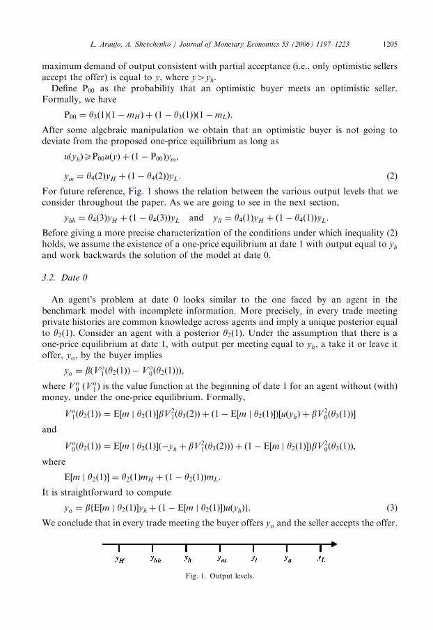
For future reference, Fig. 1 shows the relation between the various output levels that weconsider throughout the paper. As we are going to see in the next section,

yhh ¼ y4ð3ÞyH þ ð1� y4ð3ÞÞyL and yll ¼ y4ð1ÞyH þ ð1� y4ð1ÞÞyL.

Before giving a more precise characterization of the conditions under which inequality ð2Þholds, we assume the existence of a one-price equilibrium at date 1 with output equal to yh

and work backwards the solution of the model at date 0.

3.2. Date 0

An agent’s problem at date 0 looks similar to the one faced by an agent in thebenchmark model with incomplete information. More precisely, in every trade meetingprivate histories are common knowledge across agents and imply a unique posterior equalto y2ð1Þ. Consider an agent with a posterior y2ð1Þ. Under the assumption that there is aone-price equilibrium at date 1, with output per meeting equal to yh, a take it or leave itoffer, yo, by the buyer implies

yo ¼ bðVo1ðy2ð1ÞÞ � Vo

0ðy2ð1ÞÞÞ,

where Vo0 (Vo

1) is the value function at the beginning of date 1 for an agent without (with)money, under the one-price equilibrium. Formally,

Vo1ðy2ð1ÞÞ ¼ E½m j y2ð1Þ�bV 2

1ðy3ð2ÞÞ þ ð1� E½m j y2ð1Þ�Þ½uðyhÞ þ bV 20ðy3ð1ÞÞ�

and

Vo0ðy2ð1ÞÞ ¼ E½m j y2ð1Þ�ð�yh þ bV2

1ðy3ð2ÞÞÞ þ ð1� E½m j y2ð1Þ�ÞbV20ðy3ð1ÞÞ,

where

E½m j y2ð1Þ� ¼ y2ð1ÞmH þ ð1� y2ð1ÞÞmL.

It is straightforward to compute

yo ¼ bfE½m j y2ð1Þ�yh þ ð1� E½m j y2ð1Þ�ÞuðyhÞg. (3)

We conclude that in every trade meeting the buyer offers yo and the seller accepts the offer.

Fig. 1. Output levels.


Proposition 1 provides a formal characterization of the one-price equilibrium (where pt isprice at date t).

Proposition 1. There exists Zo40 such that for all mH , mL with mH �mLoZo, there exists

an equilibrium with the following features:

(i)

4W

from

In every trade meeting at date 0 po ¼ 1=yo, where yo is given by (3).
(ii) In every trade meeting at date 1 p1 ¼ 1=yh, where
yh ¼ y3ð2ÞyH þ ð1� y3ð2ÞÞyL.

(iii)
In every trade meeting at date t ðtX2Þ pt ¼ 1=yH if the economy is in the high state and
pt ¼ 1=yL if the economy is in the low state.

Proof. See Appendix A.

In the class of equilibria where transaction takes place in all trade meetings at date 1, theabove equilibrium induces the highest production. The reason is that there can be no one-price equilibrium with y above yh consistent with all sellers accepting y.Note that the price level at date 1 is higher than the price level at date 0 as long as

uðyhÞ

yh

41� bE½m j y2ð1Þ�bð1� E½m j y2ð1Þ�Þ

.

We do not have the analytical solution for the conditions under which this inequality holdsbut we analyzed its validity for a wide range of values of b and y within the interval ð0; 1Þ,given the function uðyÞ ¼ y1=2.4 In all cases we obtained that the price level at date 1 ishigher than the price level at date 0. The main intuition for this result is that, while in date0 the most pessimistic seller has a posterior y2ð1Þ, at date 1 his belief increases to y3ð2Þ. As aresult, for trade to take place in all trade meetings at dates 0 and 1, the seller must be askeda smaller amount (a higher price) at date 1.An equilibrium with only one price at date 1 exists whenever the difference between mH

and mL is not very large. Note that there are two distinct effects here. First, when mH andmL are close to each other, posteriors are not going to be very different across distinctprivate histories. This implies that, after experiencing a history OB

3 ð1Þ and forming aposterior y3ð1Þ, a buyer does not attach a very high probability that the seller faces ahistory that leads to a similar posterior. Therefore, he has less incentives to deviate and askfor a higher amount of output. This is the informational effect. Second, when mH is closeto mL, the distance between yH and yL and, as a consequence, the distance between yh andy is small (see formula 1). This effect also reduces the buyer’s incentive to deviate.In Section 5, we show that there exists a region of parameters where both equilibrium

with one price and equilibrium with price dispersion exist. As we show in the followingsections, this multiple equilibrium result emphasizes the role that the informational effectplays in our economy.

e look at the following values of the parameters: b; y 2 f0:01; 0:1; 0:5; 0:9; 0:99g. The simulations are available

the authors upon request.


4. An equilibrium where prices are informative

In what follows we describe a region of parameters where an equilibrium with pricedispersion exists. As in Section 3, we first informally discuss our main result andProposition 2 provides a formal proof.

Since information about the state of the economy is revealed at date 2, in every trademeeting from date 2 onwards the amount of output equals yH (yL) if the state of theeconomy is high (low). We now consider the formation of prices at date 1.

4.1. Date 1

An agent’s decision at date 1 depends on his private history. As in the one-price case, aprivate history includes the agent’s money holdings and the money holdings of hispartner.5 Our objective is to describe an equilibrium where the choice of the buyer dependson his private history. In particular, we expect that a buyer asks for a higher output(smaller price) if he faces the more optimistic history (OB

3 ð1Þ) and for a smaller output(higher price) if he faces the history OB

3 ð2Þ. More formally, the buyer’s strategy at date 1implies

s1BðOB3 ð1ÞÞ4s1BðO

B3 ð2ÞÞ.

Before the buyer makes an offer the only part of his private history which is not commonknowledge in the economy is the value of the first entry (just note that for both OB

3 ð1Þ andOB

3 ð2Þ the last two entries are the same). If the seller believes that the buyer follows astrategy which is history-contingent, he can use the buyer’s offer as an additional piece ofinformation which reveals his entire private history. Suppose, for example, that a sellerwith a history OS

3ð1Þ meets a buyer and the buyer asks for s1BðOB3 ð1ÞÞ. The seller knows that

a buyer only asks for s1BðOB3 ð1ÞÞ if his private history is OB

3 ð1Þ. Therefore, instead of havinga posterior y3ð1Þ, he includes the buyer’s offer into his information set and updates hisbelief to y4ð1Þ. Analogously, if a seller has a history OS

3ð2Þ and meets a buyer who asks fors1BðO

B3 ð1ÞÞ, he updates his belief from y3ð2Þ to y4ð2Þ.

Consider the problem of a buyer with a history OB3 ð1Þ who asks for s1BðO

B3 ð1ÞÞ. Moreover,

assume that he wants to target only optimistic sellers. Since he knows that these sellers aregoing to have a posterior equal to y4ð1Þ after receiving the offer, the buyer’s optimaldecision is to set

s1BðOB3 ð1ÞÞ ¼ bðV 2

1ðy4ð1ÞÞ � V 20ðy4ð1ÞÞÞ � yll ¼ y4ð1ÞyH þ ð1� y4ð1ÞÞyL.

A similar reasoning applies for a buyer that asks for s1BðOB3 ð2ÞÞ after a history OB

3 ð2Þ. Inthis case, a seller with history OS

3ð1Þ updates his belief from y3ð1Þ to y4ð2Þ. Alternatively, aseller with history OS

3ð2Þ updates his belief from y3ð2Þ to y4ð3Þ. Now assume that a buyerwith a history OB

3 ð2Þ targets all sellers and makes an offer that is always accepted. Underthe proposed strategy, the best offer he can make is to ask for

s1BðOB3 ð2ÞÞ ¼ bðV 2

1ðy4ð3ÞÞ � V 20ðy4ð3ÞÞÞ � yhh ¼ y4ð3ÞyH þ ð1� y4ð3ÞÞyL.

5Note that prices at date 0 are the same across trade meetings. Therefore, we can apply the same reasoning as

before and conclude that the only relevant piece of information an agent carries from date 0 to date 1 is his money

holdings and the money holdings of the agent he met. This implies that the set of agents’ private histories at the

beginning of date 1 are the same as in the one-price case.


The next step is to check the buyer’s incentive to follow the prescribed strategy.Consider, first, a buyer with a history OB

3 ð1Þ. If he asks for yll , his expected payoff is

P00½uðyllÞ þ bV20ðy4ð1ÞÞ� þ ð1� P00ÞbV2

1ðy4ð2ÞÞ.

There is a probability P00 that he meets a seller with a history OS3ð1Þ, in which case the latter

accepts the offer and the buyer moves to date 2 without money. There is also a probabilitythat the seller has a history OS

3ð2Þ. In this case, he rejects the offer, there is no trade and thebuyer moves to date 2 with money.If a buyer deviates from the prescribed strategy and, for example, asks for y, his payoff

depends on the seller’s belief after observing y. A necessary condition for our proposedstrategy to be an equilibrium is that, for any value of y such that yhhoypyll , onlyoptimistic sellers accept the offer. As we show in the proof of Proposition 2, this conditionis satisfied as long as the seller’s belief after observing y gives a sufficiently smallprobability to the optimistic buyer.6 Hence, the best possible deviation for an optimisticbuyer is to ask for yhh. In this case, he obtains

uðyhhÞ þ bV20ðy3ð1ÞÞ.

Note that, since all sellers accept the offer, a buyer does not gain any additionalinformation and moves to date 2 with a posterior y3ð1Þ. Hence, a buyer with a historyOB

3 ð1Þ follows the prescribed strategy as long as

P00ðuðyllÞ þ bV0ðy4ð1ÞÞÞ þ ð1� P00ÞbV1ðy4ð2ÞÞXuðyhhÞ þ bV0ðy3ð1ÞÞ.

We can rewrite this expression as

P00uðyllÞ þ ð1� P00ÞymXuðyhhÞ. (4)

Now, consider the incentive constraint faced by a buyer with history OB3 ð2Þ. A computation

similar to the one above shows that a pessimistic buyer does not deviate from theprescribed strategy and asks for yhh as long as

uðyhhÞXP01uðyllÞ þ ð1� P01Þyhh. (5)

Before providing a formal characterization of the conditions under which theinequalities in ð4Þ and ð5Þ hold, we assume that the equilibrium with price dispersion atdate 1 exists and work backwards the solution to the model at date 0.

4.2. Date 0

In every trade meeting at date 0, private histories are common knowledge and lead to theposterior y2ð1Þ. Under the assumption that the equilibrium at date 1 exhibits pricedispersion, a take it or leave it offer yd by the buyer implies

yd ¼ bðVd1ðy2ð1ÞÞ � Vd

0ðy2ð1ÞÞÞ,

where Vd0 (Vd

1) is the value function at the beginning of date 1 for an agent without (with)money, under the price dispersion equilibrium. Formally,

Vd1ðy2ð1ÞÞ ¼ E½m j y2ð1Þ�bV 2

1ðy3ð2ÞÞ þ ð1� E½m j y2ð1Þ�ÞfP00½uðyllÞ þ bV20ðy4ð1ÞÞ�

þ ð1� P00ÞbV20ðy4ð2ÞÞg

6We also prove in the Appendix that this constraint on beliefs satisfies the intuitive criterion.


and

Vd0ðy2ð1ÞÞ ¼ E½m j y2ð1Þ�fð1� P01Þ½�yhh þ bV 2

1ðy4ð3ÞÞ� þ P01bV 20ðy4ð2ÞÞg

þ ð1� E½m j y2ð1Þ�ÞbV 20ðy3ð1ÞÞ.

It is straightforward to compute

yd ¼ bfE½m j y2ð1Þ�ðð1� P01Þyhh þ P01ymÞ þ ð1� E½m j y2ð1Þ�ÞðP00uðyllÞ

þ ð1� P00ÞymÞg. ð6Þ

Therefore, if there is price dispersion at date 1, in every trade meeting at date 0 a buyeroffers yd and a seller accepts the offer. We now provide a formal characterization of theequilibrium with price dispersion (where pt is price at date t).

Proposition 2. There exists Zd4n40 such that for all mH , mL with nomH �mLoZd, there

exists an equilibrium with the following features:

(i)

7P

mH yl

optim

In every trade meeting at date 0 p0 ¼ 1=yd, where yd is given by ð6Þ.
(ii) At date 1 price dispersion arises. The distribution of prices across trade meetings is
phh ¼1

yhh

with probability mi,

where yhh ¼ y4ð3ÞyH þ ð1� y4ð3ÞÞyL.

pll ¼1

yll

with probability ð1�miÞ2,

where yll ¼ y4ð1ÞyH þ ð1� y4ð1ÞÞyL.Moreover, there is no trade with probability mið1�miÞ

i ¼ H;L.

(iii)
In every trade meeting at date t ðtX2Þ pt ¼ 1=yH if the economy is in the high state and
pt ¼ 1=yL if the economy is in the low state.


Note that, in the class of equilibria where buyers condition their behavior on privateexperiences, the above equilibrium induces the highest production. The reason is that aseller does not accept an offer y4yll , and a pessimistic seller does not accept an offery4yhh if he believes that such an offer comes from a pessimistic buyer.

As in the previous section, we can also compare output at date 0 with output at date 1.For example, if the low state of the economy is realized, we can compute the averageoutput across trade meetings at date 1 as7

mHyll þmLyhh.

recisely, we have ðð1�mLÞ2=ðð1�mLÞ

2þmLð1�mLÞÞÞyll þ ðmLð1�mLÞ=ðð1�mLÞ

2þmLð1�mLÞÞÞyhh �

l þmLyhh. For example, ð1�mLÞ2=ðð1�mLÞ

2þmLð1�mLÞÞ is the probability of a meeting between an

istic buyer and an optimistic seller given that a trade meeting is realized and the economy is in the low state.


We did not find the analytical solution for these comparisons. However, for all numericalspecifications that we considered8 we obtained that, if there is an equilibrium with pricedispersion and the low state is realized, the average level of output at date 1 is alwaysgreater than the output at date 0. Intuitively, in the low state there is a high probability oftrade meetings with output yll . If the high state is realized output at date 0 is usually largerthan the average output at date 1, which reflects low probability of trade meetings withoutput yll and high probability of trade meetings with no trade or with output yhh.

9

An equilibrium that exhibits price dispersion arises whenever the difference between mH

and mL is sufficiently large. As in the one-price case, there are two effects in action. First,when mH and mL are distant from each other, posteriors can be very different acrossdistinct private histories. This implies that, after experiencing a history OB

3 ð1Þ and forminga posterior y3ð1Þ, a buyer attaches high probability that the seller is facing a history leadingto a similar posterior. Therefore, he has an incentive to ask for a higher amount of output.Alternatively, if the buyer faces a history leading to a posterior that attaches highprobability to the high state, he prefers to be more cautious and asks for a smaller amountof output. This is the informational effect. Second, when mH is distant from mL, thedifference between yH and yL is large. As a consequence, the distance between yhh and yll isalso large. This increases the incentives for a buyer to demand a higher amount of output.

5. Price dispersion and learning

In the previous sections, we described the interaction between the informational contentof an agent’s private history and the determination of prices. In our discussion the valuesof the parameters mH and mL are important in the characterization of the regions whereone price and price dispersion arise. Histories are more or less informative depending onthe distance between these parameters. However, as we pointed out, mH and mL have notonly informational impact on the economy but also additional impact, which is due to ourassumption that money is indivisible. In what follows, we want to control for thisindivisibility effect. More precisely, we show that even for fixed values of parameters, aprivate history can become more informative as long as agents believe that prices are usedas a way to convey information about private experiences. When it happens, pricedispersion arises. The following proposition can be proved:

Proposition 3. There exists Z40 and n40 such that, for all nomH �mLoZ, both the

equilibrium with one price and the equilibrium with price dispersion exist. Moreover, prices in

these equilibria are the same as the ones described in Propositions 1 and 2.


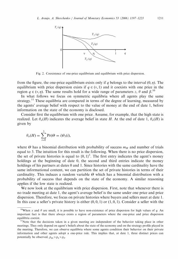
Fig. 2 illustrates the results of Proposition 3. We plot functions T1ðqÞ, T2ðqÞ and T3ðqÞ,where q ¼ mH �mL and functions TiðqÞ are defined in Appendix A. These functionsrepresent the incentive constraints for one-price and price dispersion equilibria. Inparticular, we consider uðyÞ ¼ y1=z, where z41, a functional form which satisfies ourgeneral assumptions. For Fig. 2, we assume that z ¼ 2, b ¼ 0:9 and y ¼ 0:5. As one can see

8We look at the following values of the parameters: b; y 2 f0:01; 0:1; 0:5; 0:9; 0:99g and uðyÞ ¼ y1=2. The

simulations are available from the authors upon request.9However, as the difference between mH �mL decreases, output at date 1 can become larger than output

at date 0.

ARTICLE IN PRESS

10

q

Ti (q)

T2 (q)

T1(q)

T3 (q)

ν η

Fig. 2. Coexistence of one-price equilibrium and equilibrium with price dispersion.

L. Araujo, A. Shevchenko / Journal of Monetary Economics 53 (2006) 1197–1223 1211

from the figure, the one-price equilibrium exists only if q belongs to the interval ð0; ZÞ. Theequilibrium with price dispersion exists if q 2 ðn; 1Þ and it coexists with one price in theregion q 2 ðn; ZÞ. The same results hold for a wide range of parameters z, y and b.10

In what follows we focus on symmetric equilibria where all agents play the samestrategy.11 These equilibria are compared in terms of the degree of learning, measured bythe agents’ average belief with respect to the value of money at the end of date 1, beforeinformation on the state of the economy is disclosed.

Consider first the equilibrium with one price. Assume, for example, that the high state isrealized. Let yoðHÞ indicates the average belief in state H. At the end of date 1, yoðHÞ isgiven by

yoðHÞ ¼X3i¼0

PrðY ¼ iÞy3ðiÞ,

where Y has a binomial distribution with probability of success mH and number of trialsequal to 3. The intuition for this result is the following. When there is no price dispersion,the set of private histories is equal to f0; 1g3. The first entry indicates the agent’s moneyholdings at the beginning of date 0, the second and third entries indicate the moneyholdings of his partners at dates 0 and 1. Since histories with the same cardinality have thesame informational content, we can partition the set of private histories in terms of theircardinality. This induces a random variable Y which has a binomial distribution with aprobability of success that depends on the state of the economy. A similar reasoningapplies if the low state is realized.

We now look at the equilibrium with price dispersion. First, note that whenever there isno trade meeting at date 1, the agent’s average belief is the same under one price and pricedispersion. Therefore, we focus on private histories where buyers and sellers meet at date 1.In this case a seller’s private history is either ð0; 0; 1Þ or ð1; 0; 1Þ. Consider a seller with the

10When x and y are small, it is possible to have non-existence of price dispersion for high values of q. An

important fact is that there always exists a region of parameters where the one-price and price dispersion

equilibria coexist.11Note that the decisions taken in a given meeting are independent of the behavior taking place in other

meetings. They only depend on agent’s beliefs about the state of the economy and on the strategy profile played in

the meeting. Therefore, we can observe equilibria where some agents condition their behavior on their private

information and other agents adopt a one-price rule. This implies that, at date 1, three distinct prices can

potentially be observed, phh4ph4pll .


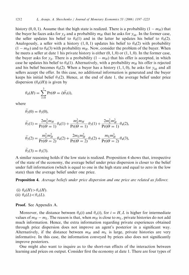
history ð0; 0; 1Þ. Assume that the high state is realized. There is a probability ð1�mH Þ thatthe buyer he faces asks for yll and a probability mH that he asks for yhh. In the former case,the seller updates his belief to y4ð1Þ and in the latter he updates his belief to y4ð2Þ.Analogously, a seller with a history ð1; 0; 1Þ updates his belief to y4ð2Þ with probabilityð1�mH Þ and to y4ð3Þ with probability mH . Now, consider the problem of the buyer. Whenhe meets a seller at date 1 his private history is either ð0; 1; 0Þ or ð1; 1; 0Þ. In the former case,the buyer asks for yll . There is a probability ð1�mH Þ that his offer is accepted, in whichcase he updates his belief to y4ð1Þ. Alternatively, with a probability mH his offer is rejectedand his belief becomes y4ð2Þ. When a buyer has a history ð1; 1; 0Þ, he asks for yhh and allsellers accept the offer. In this case, no additional information is generated and the buyerkeeps his initial belief y3ð2Þ. Hence, at the end of date 1, the average belief under pricedispersion ðydðHÞÞ is given by

ydðHÞ ¼X3i¼0

PrðY ¼ iÞ ey3ðiÞ,whereey3ð0Þ ¼ y3ð0Þ,

ey3ð1Þ ¼ 2m3LmH

PrðY ¼ 1Þy4ð1Þ þ

m2LmH


2m2Lm2

H

PrðY ¼ 1Þy4ð2Þ,

ey3ð2Þ ¼ m2Lm2

H


2mLm2H


mLm3H


ey3ð3Þ ¼ y3ð3Þ.

A similar reasoning holds if the low state is realized. Proposition 4 shows that, irrespectiveof the state of the economy, the average belief under price dispersion is closer to the beliefunder full information (which is equal to one in the high state and equal to zero in the lowstate) than the average belief under one price.

Proposition 4. Average beliefs under price dispersion and one price are related as follows:

(i)
ydðHÞ4yoðHÞ. (ii) ydðLÞoyoðLÞ.

Moreover, the distance between ydðiÞ and yoðiÞ, for i ¼ H;L is higher for intermediatevalues of mH �mL. The reason is that, when mH is close to mL, private histories do not addmuch information. Hence, the extra information regarding private experiences obtainedthrough price dispersion does not improve an agent’s posterior in a significant way.Alternatively, if the distance between mH and mL is large, private histories are veryinformative. In this case, the information conveyed by prices also does not significantlyimprove posteriors.One might also want to inquire as to the short-run effects of the interaction between

learning and prices on output. Consider first the economy at date 1. There are four types of


trade meetings, depending on the private histories of buyers and sellers. Under the one-price equilibrium, these histories are not relevant and all trade meetings generate outputequal to yh. However, under the price dispersion equilibrium, the following result arises. Ifa buyer faces the pessimistic history OB

3 ð2Þ, he asks for yhh and his offer is accepted. Ifinstead he faces the optimistic history OB

3 ð1Þ and asks for yll , his offer is accepted if theseller faced a similar history and it is rejected if the seller faced the pessimistic history. Sinceyll4yh4yhh, there are meetings in which production is higher under one price andmeetings where price dispersion is characterized by higher production.

The aggregate effect on output depends on the distribution of trade meetings acrossprivate histories, which in turn depends on the actual state of the economy. Formally, if y1

oi

ðy1diÞ is the aggregate output at date 1 under one price (price dispersion) when the state of

the economy is i ¼ H ;L, we obtain

y1oi ¼ mið1�miÞyh,

y1di ¼ mið1�miÞ½ð1�miÞ

2yll þmiyhh�,

i ¼ H ;L.

If the economy is in the high state, aggregate output under one price is greater thanoutput under price dispersion. The reason is that, under price dispersion, meetings with notrade and meetings with low production ðyhhÞ occur with high probability. However, if theeconomy is in the low state, the aggregate effect on output is ambiguous. For example, forz ¼ 2, b ¼ 0:9 and y ¼ 0:5 the one-price equilibrium dominates the price dispersionequilibrium: y1

dioy1oi. But if we assume z ¼ 2, b ¼ 0:9 and y ¼ 0:75, then we get the

opposite result. In general, output under price dispersion is higher as long as the utilityfunction is sufficiently concave and/or the prior y is sufficiently high. The reason is that, ifone of these two conditions holds, one price and price dispersion coexist at intermediatevalues of mH �mL. In this case, the extra information regarding private experiencesobtained through price dispersion significantly improves the accuracy of an agent’sposterior (see the discussion right after Proposition 4). As a result, output produced in ameeting between two optimistic agents ðyllÞ also increases. Since these meetings occur witha relatively high probability when the economy is in the low state, aggregate output ishigh.12

It is important to emphasize that price dispersion can generate more production eventhough it involves trade meetings where no trade takes place. The idea is that thepossibility of no trade acts as a punishment device against buyers who demand an outputinconsistent with their posteriors. In turn, this punishment allows optimistic buyers to askfor (and receive) a relatively high level of output. This result contrasts, for example, withJones and Manuelli (2001). They analyze an environment with asymmetric informationwith respect to the value of money and describe how a lemon’s problem arises leading tothe possibility of no trade. However, they do not consider how the possibility of no trade ina given meeting can have a positive external effect by allowing higher production in othermeetings.

12For completeness, we also considered numerically the behavior of the economy at date 0, in the region where

both one price and price dispersion equilibrium exist. For all values of b; y 2 f0:01; 0:1; 0:5; 0:9; 0:99g and for

uðyÞ ¼ y1=2 we obtain that output under the one-price equilibrium is always greater than output under price

dispersion.


Finally, one could ask whether there exists another equilibrium where prices areinformative, besides the price dispersion equilibrium. It turns out that, if the agents’ prior yis sufficiently small, there may exist another equilibrium of this form. In this equilibrium,buyers target only optimistic sellers, and ask for yl . We define and discuss this equilibriumin Appendix B. We also compare the beliefs under one price and full acceptability to thatunder one price and partial acceptability and show that in the latter the average belief iscloser to the one under full information.

6. Welfare

In this section we compare equilibrium with one price and equilibrium with pricedispersion in terms of their ex ante welfare, calculated as the agent’s expected payoff beforemoney is distributed at date 0.13 As a benchmark, let W indicates welfare in the presence ofcomplete information. We have

W ¼mð1�mÞ½uðyÞ � y�

1� b.

Welfare is maximized when the production in every trade meeting equates the marginalutility to the marginal cost (u0ðy�Þ ¼ 1). In environments with indivisible money and anupper bound on money holdings, a well-known result is that welfare in equilibrium usuallydiffers from the optimal value: both underproduction and overproduction are possible.However, as argued in Trejos and Wright (1995), it is natural to expect that y is less than y�

in a monetary economy. In our environment output in equilibrium increases with thediscount factor b and decreases with the amount of money m. As a result, when thediscount factor is high and/or the amount of money in the economy is small, output can beabove the optimal value y�. While the possibility of overproduction is not important forany of the results obtained in the previous sections, one should be careful studying thewelfare implications of the model.One way to rule out overproduction is to introduce lotteries over money, as shown in

Berentsen et al. (2002). The intuition is that a buyer can improve his expected payoff byasking for the efficient production and offering a lottery with a probability t that moneychanges hands. Berentsen et al. (2002) also show that lotteries do not eliminateunderproduction. In this case, money is always transferred with probability 1 andproduction is determined by Eq. (1). Our strategy is instead to focus on the case of theparameter values that guarantee underproduction in the region where one-priceequilibrium and price dispersion equilibrium coexist. In this case, money always changeshands with probability 1 and the results are the same as if lotteries were not present. Thisstrategy is used by Katzman et al. (2003). From Eq. (1), for any value of mH , there exists b0

such that, for all bob0, yLoy�.Let ex ante welfare be given by

W aj ¼ yW jH þ ð1� yÞW jL,

13As in the previous section, we restrict attention to efficient symmetric equilibria.


where W jH (W jL) indicates welfare in the high (low) state under the one-price ðj ¼ oÞ andprice dispersion ðj ¼ dÞ equilibrium. One can show that

Woi ¼ mið1�miÞ UðyoÞ þ bUðyhÞ þb2

1� bUðyiÞ

� �and

Wdi ¼ mið1�miÞ UðydÞ þ b½ð1�miÞ2UðyllÞ þmiUðyhhÞ� þ

b2

1� bUðyiÞ

� �,

where

UðyÞ ¼ uðyÞ � y.

Welfare is equal to the product between the number of trade meetings in every period(mið1�miÞ) and the present value of the average surplus across those meetings. Forexample, consider the average surplus at date 1 under the price dispersion equilibrium. It isequal to the probability of a meeting between an optimistic buyer and an optimistic seller(ð1�miÞ

2) times the surplus uðyllÞ � yll , plus the probability of a meeting between apessimistic buyer and a seller (mi) times the surplus uðyhhÞ � yhh. Note that, sinceinformation about the state of the economy is revealed at date 2, Woi and Wdi, only differat dates 0 and 1. Moreover, due to our assumption that mH þmL ¼ 1, the number of trademeetings does not depend on the actual state of the economy. This implies that Woi4Wdi

if and only if

UðyoÞ �UðydÞ4b½ð1�miÞ2UðyllÞ þmiUðyhhÞ �UðyhÞ�.

Since yLoy�,

UðyllÞ4UðyhÞ4UðyhhÞ.

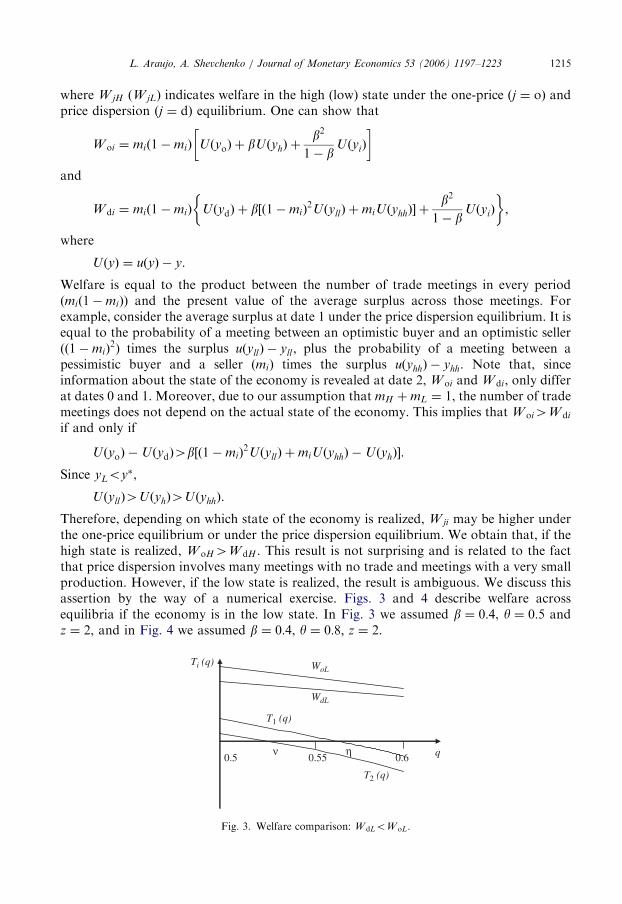
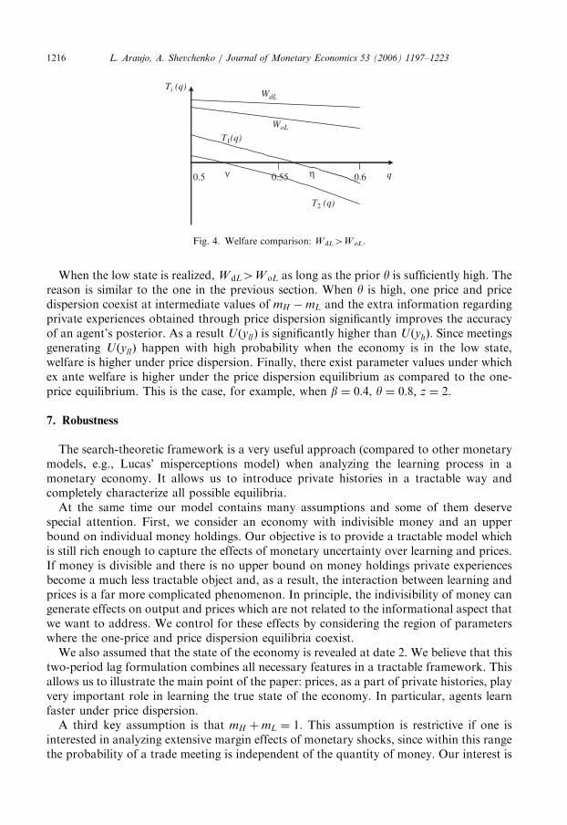
Therefore, depending on which state of the economy is realized, W ji may be higher underthe one-price equilibrium or under the price dispersion equilibrium. We obtain that, if thehigh state is realized, WoH4WdH . This result is not surprising and is related to the factthat price dispersion involves many meetings with no trade and meetings with a very smallproduction. However, if the low state is realized, the result is ambiguous. We discuss thisassertion by the way of a numerical exercise. Figs. 3 and 4 describe welfare acrossequilibria if the economy is in the low state. In Fig. 3 we assumed b ¼ 0:4, y ¼ 0:5 andz ¼ 2, and in Fig. 4 we assumed b ¼ 0:4, y ¼ 0:8; z ¼ 2.

Ti (q)

q

WoL

WdL

T1 (q)

0.550.5

T2 (q)

0.6 ην

Fig. 3. Welfare comparison: WdLoWoL.

ARTICLE IN PRESS

q

Ti (q)WdL

WoL

T1(q)

0.5 0.55 0.6

T2 (q)

ην

Fig. 4. Welfare comparison: WdL4WoL.

L. Araujo, A. Shevchenko / Journal of Monetary Economics 53 (2006) 1197–12231216

When the low state is realized, WdL4WoL as long as the prior y is sufficiently high. Thereason is similar to the one in the previous section. When y is high, one price and pricedispersion coexist at intermediate values of mH �mL and the extra information regardingprivate experiences obtained through price dispersion significantly improves the accuracyof an agent’s posterior. As a result UðyllÞ is significantly higher than UðyhÞ. Since meetingsgenerating UðyllÞ happen with high probability when the economy is in the low state,welfare is higher under price dispersion. Finally, there exist parameter values under whichex ante welfare is higher under the price dispersion equilibrium as compared to the one-price equilibrium. This is the case, for example, when b ¼ 0:4, y ¼ 0:8; z ¼ 2.

7. Robustness

The search-theoretic framework is a very useful approach (compared to other monetarymodels, e.g., Lucas’ misperceptions model) when analyzing the learning process in amonetary economy. It allows us to introduce private histories in a tractable way andcompletely characterize all possible equilibria.At the same time our model contains many assumptions and some of them deserve

special attention. First, we consider an economy with indivisible money and an upperbound on individual money holdings. Our objective is to provide a tractable model whichis still rich enough to capture the effects of monetary uncertainty over learning and prices.If money is divisible and there is no upper bound on money holdings private experiencesbecome a much less tractable object and, as a result, the interaction between learning andprices is a far more complicated phenomenon. In principle, the indivisibility of money cangenerate effects on output and prices which are not related to the informational aspect thatwe want to address. We control for these effects by considering the region of parameterswhere the one-price and price dispersion equilibria coexist.We also assumed that the state of the economy is revealed at date 2. We believe that this

two-period lag formulation combines all necessary features in a tractable framework. Thisallows us to illustrate the main point of the paper: prices, as a part of private histories, playvery important role in learning the true state of the economy. In particular, agents learnfaster under price dispersion.A third key assumption is that mH þmL ¼ 1. This assumption is restrictive if one is

interested in analyzing extensive margin effects of monetary shocks, since within this rangethe probability of a trade meeting is independent of the quantity of money. Our interest is


instead on the intensive margin effects of the interaction between prices and learning.Another advantage of the specification where mH þmL ¼ 1 is that it delivers a natural wayin which private histories reveal information about the state of the economy. Precisely, weobtain that, as private histories become more informative, i.e., as the difference mH �mL

increases, an optimistic agent increases his belief that the economy is in the low state and apessimistic agent increases his belief that the economy is in the high state. Underalternative specifications, where mH þmLa1, it can happen that optimistic agents becomemore pessimistic as the distance between mH and mL increases. We conjecture that thediscrepancy between the results under mH þmL ¼ 1 and mH þmLa1 can be eliminated ifwe consider a more general model where the short-run lasts for more than two periods andprivate histories become longer and more informative.

Finally, the main experiment in our model involves analyzing the short- and long-runeffects of varying the initial endowment of money stock. This approach may sound toostylized since what we observe in the real world are changes in the quantity of moneythrough monetary injections. In what follows we discuss some differences between thesetwo approaches and claim that our main results are robust to either specification.

First, note that the introduction of monetary injections14 implies that at date 0 all sellersstill form the same posterior regarding the state of the economy. This is so since they allfaced the same history, i.e., they started with no money, received no money through amonetary injection and met an agent with money. As a result, the take it or leave it offerassumption implies that in all trade meetings at date 0 trade occurs at the same price.Hence, this price has no informational content, as in the current framework. At date 1analysis becomes a bit harder. In particular, if there are two possible monetary injections(mH and mL) the set of private histories for the buyer (seller) becomes fOB

4 ð1Þ; OB4 ð2Þ; O

B3 ð2Þg

(fOS4ð1Þ; O

S4ð2Þ, O

S3ð2Þg). Clearly, in the environment with monetary injections, a one-price

equilibrium with full acceptability still exists at a price consistent with acceptance by themost pessimistic sellers, i.e., the ones with a belief y3ð2Þ. This happens as long as thedistance mH �mL is not too large and the intuition is the same as the one presented inSection 3. It also seems reasonable to expect that equilibria with price dispersion existunder the new specification. Since the set of private histories is larger, we believe that theremay be more than one such equilibrium. However, the main intuition from these resultsshould be the same, i.e., price dispersion increases communication and improves theprecision of the agents’ average beliefs. We also expect that, as long as the low state isrealized, there will be regions of the parameter space where price dispersion will entail ahigher ex ante welfare than the one-price equilibrium.

8. Concluding remarks

The literature on the misperceptions theory of money has always emphasized learning asa mechanism through which an economy reaches the long-run. But the modeling of alearning process has been missing in this literature, mostly because of the technicaldifficulties that arise in a dynamic framework. The main objective of this article has been tocharacterize equilibria in a dynamic monetary economy with uncertainty where agents usetheir private experiences to update their knowledge about the actual state of the economy.

14This can be done in the same way as in Wallace (1997) with a restriction to only two possible levels of

monetary injection, high (mH ) and low (mL).


Several results have been found. First, we have shown the impact of the volatility ofmonetary policy on prices. Given mL is close to mH , only the one-price equilibriumemerges in the short-run. Otherwise, price dispersion may arise. Second, we havecharacterized a region of parameters where the one-price equilibrium and the equilibriumwith price dispersion coexist. The most interesting finding is that in this region pricedispersion provides a mechanism through which agents obtain more precise informationabout the purchasing power of money. The intuition is that price dispersion allows agentsto indirectly communicate their private experiences, which increases the overall amount ofinformation. Despite the loss of output in some of the trade meetings, the aggregate outputin the economy with price dispersion may be closer to the one under complete information.As a result the price dispersion equilibrium can entail higher ex ante welfare than the one-price equilibrium. A common perception, that volatile monetary regimes may cause pricedispersion and as a result confusion about the value of money, can be misleading. Exactlythe opposite may happen. If one price emerges as an equilibrium outcome there is no wayfor agents to communicate their private histories while they trade with each other.Therefore, it may take much longer for the actual state of the economy to be revealed.

Appendix A

Proof of Proposition 1. First, since the state of the economy is revealed at date 2, we musthave

stBðjÞ ¼ yj where j ¼ H ;L; for all tX2,

stSðj; yÞ ¼

A if ypyj ;

R otherwise

�for all tX2.

Now consider the economy at date 1. Consider the following pair of functions:

s1BðOB3 ð1ÞÞ ¼ s1BðO

B3 ð2ÞÞ ¼ yh and

s1SðOS3ð1Þ; yÞ ¼

A if ypyll ;

R otherwise;

(s1SðO

S3ð2Þ; yÞ ¼

A if ypyh;

R otherwise

(and the following belief function

mðyÞ ¼1 if y4ym;12

if ypym:

(Given ðst

B;stSÞ and mðyÞ, an equilibrium with one price exists as long as

uðyhÞXP00uðyllÞ þ ð1� P00Þym, (A)

uðyhÞXP01uðyllÞ þ ð1� P01Þyhh. (B)

Since the right-hand side of (A) is bigger than the right-hand side of (B), it suffices toconsider inequality (A). First, notice that in any one-price equilibrium where tradehappens in all meetings, yh is the maximum output consistent with acceptance by all sellers.For any y above yh, acceptance by a seller with a history OS

3ð2Þ implies that this seller has aposterior below y3ð2Þ. However, in an equilibrium where all buyers ask for the same price,


prices do not affect posteriors. Hence, on the equilibrium path, a posterior of a seller withhistory OS

3ð2Þ must be equal to y3ð2Þ. Moreover, notice that yll is the maximum output thata seller with a history OS

3ð1Þ is willing to accept. This output can be reached if sellers, afterseeing a deviation to yll , attach a probability 1 that such a deviation is coming from a buyerwith a history OB

3 ð1Þ. Therefore, yll is the best possible gain that a buyer can get bydeviating from the equilibrium path. Clearly, by attaching the value 1 to the belief that theoptimistic buyer deviated when yXym, we automatically satisfy the intuitive criterion.

First, we define a function T1ðqÞ:

T1ðqÞ ¼ uðyhÞ � P00uðyllÞ � ð1� P00Þym,

where q � mH �mL. Simple calculations show that at q ¼ 0,yh ¼ yll ¼ ym ¼ yH ¼ yL ¼ y0, where y0 is the solution to the following equation:

uðyÞ ¼2� bb

y.

Then, T1ð0Þ ¼12½uðy0Þ � y0�, and as a result T1ð0Þ40 is satisfied iff uðy0Þ4y0, which is

always true. Next, notice that T1ðqÞ ! ½� uðy1Þ�o0 as q! 1, where y1 is the solution tobuðyÞ ¼ y. It means that the one-price equilibrium exists if qoZoo1, where

Zo ¼ minfq s.t. T1ðqÞ ¼ 0;T 01ðqÞo0g.

Finally, since buyers and sellers share the same posterior in a trade meeting at date 0, onlyone price can emerge in equilibrium. We have

s0BðOB2 ð1ÞÞ ¼ yo and s0SðO

S2ð1Þ; yÞ ¼

A if ypyo;

R otherwise;

(where

yo ¼ bfE½m j y2ð1Þ�yh þ ð1� E½m j y2ð1Þ�ÞuðyhÞg.

This concludes our proof. &

Proof of Proposition 2. First, since the state of the economy is revealed at date 2, we musthave

stBðjÞ ¼ yj where j ¼ H;L; for all tX2 and

stSðj; yÞ ¼

A if ypyj ;

R otherwise

(for all tX2.

Now consider the economy at date 1. We need to show that the pair of functions

s1BðOB3 ð1ÞÞ ¼ yll ,

s1BðOB3 ð2ÞÞ ¼ yhh,

sSðOS3ð1Þ; yÞ ¼

A if ypyll ;

R otherwise;

(sSðOS

3ð2Þ; yÞ ¼A if ypyhh;

R otherwise

�


and the belief function

mðyÞ ¼1 if y4ym;

0 if ypym:

(These beliefs guarantee that a seller with a history OS

3ð2Þ does not accept any offer aboveyhh. Note again that, by attaching the value 1 to the belief that the optimistic buyerdeviated when yXym, we automatically satisfy the intuitive criterion. As a result, anequilibrium with price dispersion exists if the following two inequalities are satisfied:

uðyhhÞpP00uðyllÞ þ ð1� P00Þym,

uðyhhÞXP01uðyllÞ þ ð1� P01Þyhh.

To prove the statement we define functions T2ðqÞ and T3ðqÞ:

T2ðqÞ ¼ uðyhhÞ � P00uðyllÞ � ð1� P00Þym,

T3ðqÞ ¼ uðyhhÞ � P01uðyllÞ � ð1� P01Þyhh,

where q � mH �mL. Similar to the proof of Proposition 1, at q ¼ 0,yhh ¼ yll ¼ ym ¼ yH ¼ yL ¼ y0. Then, T2ð0Þ ¼ T3ð0Þ ¼

12½uðy0Þ � y0�40 since uðy0Þ4y0.

Moreover, T2ðqÞ ! ½�uðy1Þ�o0, and T3ðqÞ ! 0 as q! 1. Notice that T3ðqÞ �

T2ðqÞ4ðP00 � P01Þ½uðyllÞ � yhh�40 for q 2 ð0; 1�. It means that equilibrium with pricedispersion exists if noqoZd, where

n ¼ minfq s.t. T2ðqÞ ¼ 0;T 02ðqÞo0g

and

Zd ¼ min

q s.t. T2ðqÞ ¼ 0;T 02ðqÞ40;

q s.t. T3ðqÞ ¼ 0;T 03ðqÞo0;

1:

8><>:Finally, since buyers and sellers share the same posterior in a trade meeting at date 0, onlyone price can emerge in equilibrium. We have

s0BðH0Þ ¼ yd and s0SðH

0; yÞ ¼A if ypyd;

R otherwise;

(where

yd ¼ bfE½m j y2ð1Þ�ðð1� P01Þyhh þ P01ymÞ þ ð1� E½m j y2ð1Þ�ÞðP00uðyllÞ

þ ð1� P00ÞymÞg.


Proof of Proposition 3. The result follows immediately after observing that T1ðqÞ �

T2ðqÞ ¼ ½uðyhÞ � uðyhhÞ�40 for all q 2 ð0; 1Þ, T1ð0Þ ¼ T2ð0Þ and T1ð1Þ ¼ T2ð1Þ. We knowfrom the proof of Proposition 2 that T3ðqÞ4T2ðqÞ, while the relationship between T3ðqÞ

and T1ðqÞ is ambiguous. Therefore, equilibria with one price and equilibria with pricedispersion coexist if noqoZ, where Z ¼ min½Zo; Zd�.This concludes our proof. &


Proof of Proposition 4. (i) We need to show thatX3i¼0

PrðYH ¼ iÞ ey3ðxÞ �X3i¼0

PrðYH ¼ iÞy3ðxÞ40.

Applying the definition of ey3ðxÞ, we obtain that this expression is equivalent to

2ð1�mH Þ½ð1�mH Þy4ð1Þ þmHy4ð2Þ � y3ð1Þ� þmH ½ð1�mH Þy4ð2Þ

þmHy4ð3Þ � y3ð2Þ�40.

After simple algebraic manipulations one can show that

ð1�mH Þy4ð1Þ þmHy4ð2Þ � y3ð1Þ40,

ð1�mH Þy4ð2Þ þmHy4ð3Þ � y3ð2Þ40

as long as

ðmH �mLÞ240.

(ii) We need to show thatX3i¼0

PrðYL ¼ iÞ ey3ðxÞ �X3i¼0

PrðYL ¼ iÞy3ðxÞo0.

Applying the definition of ey3ðxÞ, we obtain that this expression is equivalent to

2ð1�mLÞ½ð1�mLÞy4ð1Þ þmLy4ð2Þ � y3ð1Þ� þmH ½ð1�mH Þy4ð2Þ

þmHy4ð3Þ � y3ð2Þ�o0.

Again, it is straightforward to show that

ð1�mLÞy4ð1Þ þmLy4ð2Þ � y3ð1Þo0,

ð1�mLÞy4ð2Þ þmLy4ð3Þ � y3ð2Þo0

as long as

ðmH �mLÞ240.


Appendix B

In this appendix, we provide the conditions under which there exists an equilibrium withone price and partial acceptability by sellers. First, from date 2 on, price in equilibriumequals 1=yH ð1=yLÞ depending on whether the high (low) state is realized. Now consider theeconomy at date 1. We need to show that the pair of functions

s1BðOB3 ð1ÞÞ ¼ s1BðO

B3 ð2ÞÞ ¼ yl ; sSðOS

3ð1Þ; yÞ ¼A if ypyl ;

R otherwise;

(

sSðOS3ð2Þ; yÞ ¼

A if ypyh;

R otherwise

(


together with the belief function

mðyÞ ¼12 if yXyl ;

0 otherwise

(are part of an equilibrium. Notice that, according to m, after seeing a deviation y below yl ,sellers attach probability 1 that the deviant buyer has history OB

3 ð2Þ. Since pessimisticbuyers have more incentive to deviate and ask for yoyl , the proposed beliefs are consistentwith the intuitive criterion. We obtain the pair fs1B;s

1Sg and the belief function m are part of

an equilibrium iff

P01uðylÞ þ ð1� P01ÞyhhXuðyhhÞ and P00uðylÞ þ ð1� P00ÞymXuðyhhÞ.

Finally, since buyers and sellers share the same posterior in a trade meeting at date 0,only one price can emerge in equilibrium. Notice that the above equilibrium induces thehighest production in the class of equilibria involving one price and partial acceptability bysellers. Moreover, it can be easily shown that the equilibrium with one price and partialacceptability cannot coexist with the equilibrium with price dispersion. Formally, in theequilibrium with price dispersion the following inequality must hold:

uðyhhÞXP01uðyllÞ þ ð1� P01Þyhh.

However, since

P01uðyllÞ þ ð1� P01Þyhh4P01uðylÞ þ ð1� P01Þyhh

and an equilibrium with one price and partial acceptability implies

P01uðylÞ þ ð1� P01ÞyhhXuðyhhÞ

we have

uðyhhÞ4uðyhhÞ,

a contradiction. We conclude that there exists a region where both the equilibrium withprice dispersion and the equilibrium with one price and full acceptability coexist, but theequilibrium with one price and partial acceptability does not exist.We can also compute the average belief under one price and partial acceptability. We

proceed in a way similar to the analysis for the equilibrium under price dispersion. Assumethat the high state is realized. First, we can focus on private histories where buyers andsellers meet at date 1. In this case a buyer’s private history is either ð0; 1; 0Þ or ð1; 1; 0Þ.Consider a buyer with the history ð0; 1; 0Þ, hence a belief y3ð1Þ. Assume that the high state isrealized. There is a probability ð1�mH Þ that the seller he faces accepts the offer yl and aprobability mH that the seller rejects the offer. In the former case, the buyer updates hisbelief to y4ð1Þ and in the latter case he updates his belief to y4ð2Þ. A similar analysis impliesthat a buyer with a history ð1; 1; 0Þ updates his belief to y4ð2Þ upon meeting a seller thataccepts the offer yl . Moreover, he updates his belief to y4ð3Þ after meeting a seller thatrejects the offer yl . Hence, at the end of date 1, the average belief under one price andpartial acceptability ðypðHÞÞ is given by

ypðHÞ ¼X3i¼0

PrðY ¼ iÞ by3ðiÞ,


whereby3ð0Þ ¼ y3ð0Þ,

by3ð1Þ ¼ m3LmH


2m2LmH


m2Lm2

H


by3ð2Þ ¼ m2Lm2

H


2mLm2H


mLm3H


by3ð3Þ ¼ y3ð3Þ.

A similar reasoning applies if the low state is realized. It is straightforward to show that,irrespective of the state of the economy, the average belief under one price and partialacceptability is closer to the belief under full information than the average belief under oneprice and full acceptability. The proof is essentially the same as the proof of Proposition 4,replacing ey3ð1Þ with by3ð1Þ and ey3ð2Þ with by3ð2Þ.References

Araujo, L., Camargo, B., 2005. Monetary equilibrium with decentralized trade and learning. Department of

Economics Research Report #2005-1, The University of Western Ontario.

Barro, R., King, R., 1984. Time-separable preferences and intertemporal substitution models of business cycles.

Quarterly Journal of Economics 99, 817–839.

Berentsen, A., Molico, M., Wright, R., 2002. Indivisibilities, lotteries and monetary exchange. Journal of

Economic Theory 107, 70–94.

Burdett, K., Judd, K., 1983. Equilibrium price dispersion. Econometrica 51 (4), 955–970.

Cho, I., Kreps, D., 1987. Signaling games and stable equilibria. Quarterly Journal of Economics 102, 179–221.

Jones, L.E., Manuelli, R.E., 2001. Volatile policy and private information: the case of monetary shocks. Journal

of Economic Theory 99, 265–296.

Katzman, B., Kennan, J., Wallace, N., 2003. Output and price level effects of monetary uncertainty in a matching

model. Journal of Economic Theory 108, 217–255.

Lucas Jr., R.E., 1972. Expectations and the neutrality of money. Journal of Economic Theory 4, 103–124.

Lucas Jr., R.E., 1996. Nobel lecture: money neutrality. Journal of Political Economy 104 (4), 661–682.

Rob, R., 1985. Equilibrium price distributions. Review of Economic Studies 52, 487–504.

Shi, S., 1995. Money and prices: a model of search and bargaining. Journal of Economic Theory 67, 467–496.

Stigler, G., 1961. The economics of information. Journal of Political Economy 69, 213–225.

Trejos, A., Wright, R., 1995. Search, bargaining, money, and prices. Journal of Political Economy 103 (1),

118–141.

Wallace, N., 1997. Short-run and long-run effects of changes in money in a random-matching model. Journal of

Political Economy 105 (6), 1293–1307.

Wolinsky, A., 1990. Information revelation in a market with pairwise meetings. Econometrica 58 (1), 1–23.

Documents

Price dispersion, information and learningaraujolu/Price Dispersion, Information and... · Price dispersion, information and learning$ Luis Araujoa,b, ... actual quantity of goods