Embed Size (px)
Citation preview
Number of Sellers, Average Prices, and Price Dispersion
John M. Barron†
Department of Economics Purdue University
W. Lafayette, IN 47907-1310 [email protected]
Beck A. Taylor Department of Economics
Baylor University Waco, TX 76798-8003 [email protected]
John R. Umbeck Department of Economics
Purdue University W. Lafayette, IN 47907-1310 [email protected]
Forthcoming, International Journal of Industrial Organization Abstract: A variety of models provide differing predictions regarding the effect of an increase in the number of competitors in a market (seller density) on prices and price dispersion. We review different approaches to generating equilibrium price dispersion and then empirically estimate the relationship between seller density, average product price, and price dispersion in the retail gasoline industry using four unique gasoline price data sets. Controlling for station-level characteristics, we find that an increase in station density consistently decreases both price levels and price dispersion across four geographical areas. JEL Codes: L13, D43, D83 Key Words: search costs; price dispersion; retail gasoline
† Corresponding author is John M. Barron. Ph. 765-494-4451; Fax 765-494-9658.
1
Number of Sellers, Average Prices, and Price Dispersion
I. Introduction
It has been shown theoretically that price dispersion can result under a variety of different
circumstances. Some suggest that dispersion arises as a simple extension of standard
monopolistic competition. Others adopt a search-theoretic framework that suggests price
dispersion is generated when some consumers do not know the location of a low price. Both
approaches are widely accepted, yet their predictions sometimes diverge concerning the
correlation between the number of sellers in a market and the moments of the resulting
equilibrium distribution of prices.
Intuition might suggest that in markets more densely populated with buyers, the resulting
higher number of sellers would be associated with a “more competitive” market, characterized
by lower prices and less price dispersion. These associations do appear in modifications of the
standard models of monopolistic competition that allow for price variation across sellers.
However, this is not necessarily the case for models that adopt the search-theoretic approach to
price dispersion. For instance, Rosenthal (1980) finds conditions under which “increasing the
number of sellers … induces [an increase] in the sellers’ … equilibrium [price] distribution”
(p.1579). If markets with fewer sellers have higher search costs, then Samuelson and Zhang
(1992) develop a model in which “as search costs increase, prices and price dispersion may
decrease” (p.55). Lest one thinks that such models are isolated and special cases, consider the
well-known paper by Stiglitz (1987) whose very title “Are Duopolies More Competitive than
Atomistic Markets?” highlights the potential for “counter-intuitive” results, namely that markets
2
with a larger number of competitors may have higher prices, with the result depending on
assumptions regarding search costs.1
Given this theoretical ambiguity, the purpose of this paper is two-fold. First, we highlight
the sources of the conflicting theoretical predictions. Section II reviews the approaches to
generating an equilibrium price distribution based on monopolistic competition and on search-
theoretic models. For the monopolistic competition approach, we develop two alternative
modifications of the classic model presented by Perloff and Salop (1985). For the search-
theoretic approach, we consider a variant of Carlson and McAfee (1983), a model based on
optimal sequential search by consumers with heterogeneous search costs, and Varian’s (1980)
model of sales that generates a mixed-strategy pricing equilibrium. In each model, the number
of sellers in the market is determined by a zero-profit condition, and a change in the number of
sellers occurs if there is a change in market size (in terms of the number of consumers) or a
change in the fixed costs of production. For each of the four models considered, we derive the
predicted correlation between a change in the number of sellers (seller density) and the first two
moments of the equilibrium price distribution, namely the average price in the market and the
level of price dispersion.
The second purpose of this paper, presented in Section III, is to use four unique and
comprehensive firm-level data sets from the retail gasoline industry to estimate the relationships
between seller density and the level and dispersion of gasoline prices. The empirical literature
that addresses associations between seller density, average prices, and price dispersion is
relatively small when compared to the vast theoretical work on the subject, in part because of
problems related to market definition, access to firm-level data that could be used to distinguish
1 The intuition behind Stiglitz’s seemingly odd result is that, given the common search-model assumption that
searchers know the distribution of prices but not the location of specific prices, an increase in the number of
competitors makes it more costly for searchers to find a low-cost seller.
3
differences in product characteristics, and a researcher’s ability to survey all of the relevant
prices and market conditions at a single point in time. Fortunately, our empirical work relies on
four data sets that contain information on the location and characteristics of the over 3,000
gasoline stations in the San Diego, San Francisco, Phoenix, and Tucson areas. Further, the
prices contained in each of the data sets were collected on a single day, so that we have four
complete “census” price surveys. Our data provide us with a rare opportunity to examine the
relationships between the number of competitors, average product prices, and price dispersion
for a frequently-purchased, homogeneous product.
Controlling for station-level differences, we find convincing evidence across all four
geographic areas that in markets with a higher number of sellers, there is a statistically
significant, albeit modest, decrease in both the mean price and price dispersion for regular
unleaded gasoline. This evidence is consistent with variants of the standard models of
monopolistic competition, but is at odds with some of the predictions of widely cited search-
based price dispersion models. In the conclusion, we suggest some features that could be added
to often-used search-theoretic approaches to improve their ability to explain what we observe.
II. Models of Equilibrium Price Dispersion
In this section, we contrast the predicted relationship between the number of sellers (seller
density) and moments of the equilibrium price distribution, namely the average price and the
extent of price dispersion, for a variety of models that generate an equilibrium price distribution.
Our goal is to identify and provide insight regarding the potentially conflicting predictions of
these models, and thus set the stage for our subsequent empirical analysis. Although there are
substantive differences in the key assumptions of the various models considered, there are
common elements as well, so we begin by introducing these common features.
4
A. Common Elements of the Models
Let ≥N be the total number of sellers in the market. For seller i, production of units
of output involves a common fixed cost component k, and a constant marginal cost component
2 iq
iα . That is,
( )i i iC q k qiα= + , (1)
where and 0>k 0>iα , i = 1, …, N. Let there be L buyers in the market, each purchasing one
unit of the good. Let consumer j’s value of the good offered by seller i, jiθ , equal a common
reservation value, r, minus a “visiting” or “search” cost, , such that jiv ji r v= − jiθ .2 For
consumer j, the gain to purchasing the product from seller i at price is then ip
ji ji iu r v p= − − . (2)
If prices are known and consumers consider the good to be differentiated across sellers, then
consumer j’s visiting cost for seller i can be viewed as being drawn from the non-degenerate
distribution . This is the setting of monopolistic competition models. Note that we follow
Anderson and de Palma’s (2001) generalization of Perloff and Salop (1985) in allowing
consumer j’s realized value of the good offered by seller i,
( )iF v
ji ijr vθ = − , to be drawn from a
2 This specific form is chosen so that we can use common notation to represent both the monopolistic competition
and the search-theoretic models. Although subsequent discussions attribute variations in value to variations in
“visiting” costs, such variations in value could easily be more broadly interpreted to reflect a variety of factors that
might influence individuals’ preferences. For simplicity, we assume the upper bound of the distribution of such
visiting costs is sufficiently low that all consumers in the market will purchase one unit of the good from one of the
sellers in the market at equilibrium prices.
5
distribution that can vary across sellers.3 Section B below considers the emergence of an
equilibrium price distribution in this setting.
If prices are not known until the consumer visits a seller, and consumers consider the good
to be homogenous across sellers, then consumer j’s common cost of visiting any seller is a single
draw from the distribution . This is the setting of many search-theoretic models. Section C
below considers the emergence of an equilibrium price distribution in this alternative framework.
The models described in Sections B and C have in common a zero-profit condition to determine
the equilibrium number of sellers in the market.
( )F v
B. Monopolistic Competition and Equilibrium Price Dispersion
Monopolistic competition arises when consumers perceive differentiated products across
sellers. The standard monopolistic competition model assumes all sellers have the same realized
marginal cost ( ) and that there is a common distribution across sellers from which each
consumer draws the visiting cost for the good offered by each seller ( ). As Perloff
and Salop (1985) have shown, such symmetry assumptions can result in a single equilibrium
price with expected sales by each seller equal to L/N. The zero-profit condition then determines
the number of sellers, with the resulting equilibrium characterized by an identical price at all
αα =i
( ) ( )iF v F v=
3 There is, however, a difference in how we characterize seller heterogeneity from Anderson and de Palma (2001).
Anderson and de Palma define the value of seller i’s good to consumer j by ji iq jiθ ε= + , where is a measure of
product quality and
iq
jiε is a random variable i.i.d. across sellers. Thus, in terms of our notation, Anderson and de
Palma focus on differences across sellers in the mean of the distribution of visiting costs, ( )iF v . Our more general
notation allows us to also consider differences across sellers in terms of the variance of the visiting cost distribution,
and in fact we focus on this latter source of seller heterogeneity. In other words, in Anderson and de Palma, seller
heterogeneity reflects quality differences, while our seller heterogeneity reflects differences in consumer value
heterogeneity across different types of sellers.
6
sellers equal to the common marginal cost, α , plus average fixed cost, k/(L/N). Thus,
equilibrium price dispersion in the standard monopolistic competition model will require the
introduction of asymmetry across firms.
Two types of asymmetry are suggested for generating equilibrium price dispersion in a
monopolistic competition model. One method of introducing asymmetry is to assume
heterogeneity in the distribution of visiting costs across sellers that can result in differences in
sellers’ price elasticities of demand if all sellers were to charge the same price. Walsh and
Whelan (1999), among others, have adopted the assumption of heterogeneous demand elasticity
as a key source of price dispersion. A second method of introducing asymmetry is to assume
heterogeneity across sellers in their realized marginal production cost. We consider below the
implications of these two types of asymmetry for the relationship between seller density and
moments of the price distribution.
1. Monopolistic competition: Heterogeneous seller demand
Consider a monopolistic competition model in which the prices charged by different sellers
are known to all consumers, the realized marginal production costs are identical across sellers,
but the distribution of “visiting costs” is not symmetric across sellers. In particular, sellers can
be divided into groups, and for any two sellers who are in different groups, say sellers i and k,
. Under these conditions, differences in price elasticity across sellers means that
identical prices for all sellers will not satisfy the standard profit-maximizing conditions
)()( vFvF ki ≠
iii mp α= , i = 1, …, N, (3)
where ( ) 11 >−= iii eem , and e )/)(/( iiiii qppq ∂∂−= is seller i’s price elasticity of demand.
The implication is that the equilibrium will be characterized by the non-degenerate price
distribution, G . )( p
7
With heterogeneous demand, some sellers will make more profit than others. We assume
that upon entering the market, sellers are assigned one of D demand-influencing distributions of
visiting costs for potential customers. The number of sellers who participate in the market each
period, N, is then determined such that sellers with fixed cost k and marginal cost α expect zero
profit if one of the D distributions is randomly assigned, and then the N sellers solve for the Nash
equilibrium prices as given by (3).4 Note that we assume D, the number of different types of
visiting cost distributions attached to sellers in the market, is fixed such that changes in the
number of sellers will not alter the set of visiting cost distributions across sellers.
Now consider the potential change in the average price and price dispersion, as measured by
the price variance, associated with an increase in the number of sellers that can arise either due
to an increase in the number of consumers, L, or a reduction in the fixed cost, k. Perloff and
Salop (1985) show that for the symmetric-demand case, such an increase in the number of sellers
tends to increase the price elasticity of demand, decrease the markup, and thus lower the
equilibrium price.5 For the asymmetric-demand case, holding constant the number of different
seller types, D, a reasonable extension of the analysis suggests that the increase in the number of
sellers of each type will also tend to increase the price elasticity across sellers, and thus reduce
markups and prices. This reduction in markups for sellers toward zero suggests, given a
4 Our assumption that a firm’s entry decision is made prior to the realization of specific demand characteristics from
one of D potential demand-influencing distributions of visiting costs for potential customers, while admittedly
somewhat artificial, is one way to assure markets of different sizes have similar demand characteristics.
5 Perloff and Salop (1985) provide specific conditions for the limiting result that price approaches marginal cost as
the number of firms becomes very large. Anderson, de Palma, and Nesterov (1995) demonstrate the importance of
log-concavity of the density of visiting costs to ensure that the equilibrium price does not increase with the number
of firms.
8
common marginal cost, that the variance in markups would decrease with an increase in the
number of sellers, and thus there would be reduced price dispersion.6
There is also a potential indirect effect of a change in seller density that can arise if we
assume that each consumer in the market considers visiting a fixed subset of sellers C N< . In
this case, an increase in the number of sellers within a specific geographic region can lower the
range of costs to a consumer “visiting” the C closest sellers. If the original costs for consumer j
of visiting one of the C closest sellers are , i = 1. … , C, then a higher density of sellers
suggests new visiting costs , with 1
ojiv
ojiji vv β= 0>> β . This change can be interpreted as a
reduction in consumers’ preference intensity for particular sellers. Perloff and Salop show for
the symmetric case, and we would expect it to hold for the asymmetric case as well, that such a
reduction in consumers’ preference intensity implies, other things equal, a larger price elasticity
of demand for sellers, and thus a reduced markup for sellers. If this is the case, then an increase
in the number of sellers can also be linked to a reduction in the average price in the market as
well as to a reduction in price dispersion through a reduction in consumers’ preference intensity.
2. Monopolistic competition: Heterogeneous seller costs
Now consider a monopolistic competition model in which prices charged by different sellers
are known to consumers, the distribution of “visiting costs” is symmetric across consumers and
sellers ( for firms i = 1, … , N), but sellers’ marginal costs are drawn from the non-
degenerate distribution
( ) ( )iF v F v=
)(αM , such that realized marginal costs differ across firms. Given the
6 Factoring in the zero-profit constraint, if the increase in the number of sellers is due to an increase in market size,
then the lower equilibrium price implies an increase in the number of consumers per seller. On the other hand, if
the increase in the number of sellers is due to lower fixed costs, then the increase in the number of sellers will be
accompanied by a reduction in the number of consumers per seller. Recall that we assume the purchase of one unit
of the good by each consumer, and that visiting costs are such that all consumers purchase the good from one of the
sellers.
9
symmetry assumption with respect to sellers’ visiting cost distributions, we know that if all
sellers charged the same price, then price elasticities and markups would be identical across
firms. However, the realized production cost asymmetry implies that the optimal price-setting
condition in (3) would not hold for all sellers. Thus, in equilibrium, there will be differences in
prices across sellers.
As before, an increase in the number of sellers can be induced either by an increase in
market size (as measured by the number of consumers, L) or by a decrease in the fixed cost, k.
The resulting increase in the price elasticity of demand for each seller will result in a decrease in
the average markup, and thus a reduction in the average price in the market. A reduction in price
dispersion is also suggested, as the increase in price elasticity forces prices of all sellers toward
their respective marginal costs. In the limit, price dispersion will tend toward the underlying
dispersion in marginal cost, with sales increasingly skewed toward sellers with relatively low
marginal costs.
C. Search and Equilibrium Price Dispersion
A second approach to generating equilibrium price dispersion adopts a search-theoretic
framework. We consider two types of search models that generate price dispersion. The first, a
close variant of the model developed by Carlson and McAfee (1983), adopts the often-used
search paradigm that consumers know sellers’ pricing strategies and the resulting distribution of
prices, but not the location of specific prices. For a finite number of sellers, Carlson and McAfee
then rely on heterogeneity in visiting costs across consumers and heterogeneity in production
costs across firms to generate an equilibrium price distribution.7
7 Hogan (1991) is an example of a paper that adopts the Carlson and McAfee (1983) approach. There are, of
course, other assumptions that can give rise to an equilibrium price dispersion in a search-based model. For
instance, Reinganum (1979) replaces heterogeneity in consumer search costs with heterogeneity in ex post
10
The second type of search model we consider was introduced by Varian (1980) and further
developed by Stahl (1989, 1996), Guimãraes (1996), and others. Again, consumers know
sellers’ pricing strategies and the resulting distribution of prices charged. A specific form of
heterogeneity in visiting costs across consumers is assumed, namely that some consumers face
very low costs to visit additional sellers while other consumers incur very high search costs to
visiting more than one seller. If one picks appropriate search cost levels for the two groups, the
result is that consumers are divided into two groups: the “informed” who have sufficiently low
search costs such that they search all firms, learn the prices at the N sellers, and purchase from
the lowest-priced seller, and the “uninformed” who have sufficiently high search costs that they
find it too costly to visit more than one seller. Given that sellers have identical production costs,
the resulting price distribution reflects a Nash mixed-strategy pricing equilibrium.
1. Search-theoretic: Heterogeneous seller costs and heterogeneous visiting costs
Search-theoretic models like that developed by Carlson and McAfee (1983), hereafter
referred to as C&M, assume a non-degenerate distribution of producers’ marginal costs, )(αM ,
and consumers that differ in their common visiting or “search” cost to discover the price charged
by each seller. C&M characterize these differential search costs across consumers by assuming
that the distribution of visiting costs, , is uniform over the support [ . In this context,
C&M show that the price elasticity of demand is higher, and thus the markup is lower, for
higher-cost (price) firms in the market.8 The higher elasticity at high cost (price) firms follows
)(vF ],0 T
consumer purchases arising from differences in realized prices through search to generate a price distribution.
Taking a different tack, Burdett and Judd (1983) introduce the possibility for a consumer to sample more than one
price at a time, resulting in heterogeneity across consumers who visit a particular firm in terms of the number of
other prices sampled. Coupled with declining average costs, these conditions can generate an equilibrium price
distribution with several prices generating identical profits.
8 For more details, see Carlson and McAfee (1982, 1983).
11
from the fact that the change in quantity for a given price change is identical across firms, but the
ratio of price to quantity is higher at higher-cost (price) firms.
In determining the number of sellers in the market, C&M assume zero fixed costs and order
sellers by marginal cost. Sellers are ordered by production costs, and the equilibrium number of
sellers in a market is determined by those sellers who can generate a non-negative profit in the
market. The marginal seller earns a profit, but the next highest-cost seller, if it were to enter,
would not earn positive profits. If we were to adopt C&M’s entry condition, then the cost
distribution of the sellers in the market would differ with market size, with a larger market
having, on average, higher-cost sellers. One way to avoid this issue is to introduce a fixed cost
component and an entry condition that involves zero expected profit given the subsequent,
random assignment of marginal costs drawn from the distribution )(αM . As a result, an
increase in the number of sellers will not alter the equilibrium price distribution through a
change in the underlying distribution of marginal production costs.
Now consider the change in the price distribution when the number of sellers increases, due
either to an increase in the number of buyers, L, or a decrease in fixed cost, k. The analysis of
C&M indicates that with the increase in sellers, there will be reduced markups and thus a lower
average price.9 For the case of a larger market size, similar results are also found by Stiglitz
(1987), who notes that although a change in price induces a smaller proportion of consumers to
alter their search if the number of firms in the market is larger, this is more than offset by the fact
that there are relatively more consumers potentially affected. So, what does the analysis predict
9 For the case of an increase in market size, we know from the zero-profit condition that the increase in the number
of firms will be proportionately less than the increase in the number of customers, such that the lower average price
is offset by an increase in expected sales. However, this does not alter the prediction that markets with a larger
number of sellers will have lower prices. For the case of an increase in the number of firms due to lower fixed
costs, the average number of customers decreases across firms.
12
concerning the relationship between the number of sellers and price variance? In C&M’s words,
“somewhat surprisingly, the answer is that [the price variance] increases” (p. 490). They note,
however, that there is an upper bound in the price variance determined by the variance in the
underlying distribution of marginal production costs.
As in our discussion of monopolistic competition models, there is also a potential indirect
effect of a change in seller density that can arise if each consumer in the market considers
visiting only a fixed subset of sellers C N< . In this case, a lower range of “visiting” or search
costs can accompany an increase in the number of sellers within a specific geographic region. In
C&M’s model, such a decrease in the range of search costs alone increases the price elasticity of
demand faced by individual sellers, and thus leads to lower markups and a reduction in the
average price.10 However, such a reduction in search costs implies no change in price variance.
2. Search theoretic: Heterogeneous visiting costs and some informed consumers
10 Carlson and McAfee is but one example of the common finding in the search literature that a reduction in search
costs across consumers results in an increase in the responsiveness of quantity demanded to a change in price. For
instance, see Stiglitz (1987), Samuelson and Zhang (1992), Rosenthal (1980), and Varian (1980). However, this
finding is not universal. Samuelson and Zhang (1992) construct a model in which heterogeneous consumers have
differing valuations for the products of different firms and must search for both price information and information
concerning the characteristics of firms’ goods which affect their valuations. Firms are assumed to have asymmetric
costs of production. Like the Carlson and McAfee model, a reduction in search costs leads to increased sensitivity
of consumers to price changes. However, Samuelson and Zhang claim that a more “competitive” market, as
measured by lower search costs, can lead to higher prices and increased price dispersion. Samuelson and Zhang
have lower search costs inducing increased participation in the market as well. This introduces the potential for a
decrease in search costs to reduce the price elasticity of demand as it increases the number of consumers visiting
each firm, and thus increases the pool of consumers from whom the firm can potentially extract surplus. In their
example, they show that this scale effect can dominate, such that lower search costs lead to higher prices and
increased price dispersion.
13
In contrast to C&M’s assumption of a range of search costs across buyers, the model
proposed by Varian (1980) can be interpreted as assuming a distribution of visiting or search
costs that divides potential consumers into only two groups: those with low search costs who
canvass all sellers and buy only from the lowest-priced seller (the “informed” buyers) and those
with search costs sufficiently high that they purchase from the first seller encountered, with any
seller equally likely to be contacted by one of these “uninformed” buyers. Letting I and U
respectively denote the number of informed and uninformed buyers, we have L = I + U.
A second difference from C&M is that Varian assumes that all sellers have identical
marginal costs. The result is an equilibrium characterized by randomized pricing strategies.
Each seller determines price by drawing from the distribution of potential prices, G(p).
Naturally, all prices offer the same expected profit; a lower price reduces the returns from sales
to the uninformed, but this is exactly offset by the increase in expected returns arising from the
increased likelihood that the seller will be the lowest-priced seller, and thus sell to all of the
informed consumers.
In the Varian approach, unlike C&M, a higher number of sellers, due either to a higher
number of buyers (with no change in the proportion of informed buyers) or lower fixed costs, is
linked to a higher average price. The explanation for this seemingly odd result is that an increase
in the number of sellers reduces the likelihood that a given price captures the informed
consumers. Given sellers’ tendency to discriminate in pricing and charge either a low price to
attract the informed buyers or a higher price to exploit the uninformed, the relative reduction in
the potential success of the former strategy leads to an overall increase in the average price.11
11 Stahl (1989) explicitly highlights this result for the Varian-type model. Stiglitz (1987) also recognized this
possibility, noting that in the case of non-linear search costs, one may obtain the counterintuitive result that prices
rise as a result of entry.
14
Simulations of Varian’s model also indicate an increase in variance can accompany the increase
in the number of sellers.12
With respect to the potential indirect effect of a higher number of sellers on search costs, our
first step is to interpret such a change in search costs in the context of the Varian-type model,
one in which we have informed and uninformed buyers. In this context, a decrease in the range
of search costs can be viewed as increasing the proportion of buyers who are “informed.” Such a
change will clearly reduce the average price. However, simulations indicate that the effect on
price variance is ambiguous, as the variance tends to fall for very low and very high proportions
of buyers who are informed. 13
Interestingly, Rosenthal (1980), in a model similar to that of Varian, also arrives at the result
that a more “competitive” market can result in an increase in the average price, where more
competitive is defined in terms of an increase in the number of sellers. However, Rosenthal’s
result differs from our discussion above in that Rosenthal assumes an increase in the number of
sellers to mean that, on average, a seller’s customers are less likely to be drawn from the pool of
low-search-cost consumers. Thus, Rosenthal’s analysis implicitly reduces the proportion of
buyers who are informed with an increase in the number of sellers. As we have seen, the result
of such a change in “search costs” can affect prices independent of a change in the number of
sellers in the market.
III. An Empirical Analysis of Retail Gasoline Markets
We are now able to motivate the empirical work to follow. We start by assuming that the
reason markets differ in the density of sellers is related to differences either in market size, in
12 Our simulations parallel simulations provided in Varian (1980), and the results appear to be robust to various
parameter values.
13 Varian also noted this ambiguous effect in simulations provided in his paper.
15
terms of the number of consumers L, or in the fixed production cost, k. Table 1 summarizes our
previous discussion regarding the suggested correlations between seller density and the moments
of the price distribution, and between the range of search costs and the moments of the price
distribution.14
According to either of the two monopolistic competition (product differentiation) models of
price dispersion considered above, the suggested correlations between seller density and
moments of the price distribution are identical: in markets with higher seller density, there will
be a lower average price and decreased price dispersion. This relationship is reinforced if we
link higher seller density to a lower range of visiting costs.
In contrast, the search-theoretic approach of Carlson and McAfee (1983) indicates that with
a higher seller density, there will be a lower average price but a higher price variance. If we link
higher seller density to lower search costs, this reinforces the negative correlation between seller
density and the average price, but the variance relationship remains intact, as changes in search
costs per se have no effect on variance.
The Varian-type search-theoretic model of price dispersion suggests that a larger number of
sellers will be associated not only with a higher price variance, but also with a higher average
price. If the reduction in search costs that can accompany an increase in seller density is
interpreted as an increase in the proportion of informed individuals, then this provides an
offsetting result with respect to the seller density/average price relationship, as an increase in the
proportion of informed consumers reduces the average price. However, the potential offset from
the indirect effect for the seller density/price variance relationship is less clear, as an increase in
the proportion of informed consumers can lead to either a higher or lower variance in prices,
depending on the model’s parameters.
14 Recall that for the Varian-type model, a reduced range of search costs is interpreted as an increase in the
proportion of consumers that are informed.
16
Thus, the predicted correlation between the number of sellers (seller density) and either the
average price or price variance depends on the model we choose and the importance we attach to
the idea that higher seller density reduces search costs. With this in mind, we now turn to the
empirical analysis to determine if a clear relationship can be established in real markets, namely
retail gasoline markets. We start with a review of the empirical literature, and then present our
empirical analysis.
Three previous studies have examined price dispersion in the retail gasoline market. Using
city-level data, Marvel (1976) finds support for increased frequency of search (proxied by a
larger volume of purchases) and lower search costs (measured by greater correlation of
successive prices in the price distribution) to reduce prices and price dispersion. Png and
Reitman (1994), using Shepard’s (1991) station-level data from Massachusetts, find evidence
that stations differentiate themselves on the basis of consumers’ willingness to wait in line to buy
gasoline. Contrary to Marvel’s results, however, they find that prices are more dispersed in
markets with a greater number of competitors, supporting their service-time differentiation
hypothesis. Finally, Adams (1997), using a sample of 20 convenience stores that sell gasoline,
finds that grocery items sold in the convenience stores have a higher degree of price dispersion
than gasoline. Adams attributes this difference to the higher search costs associated with
purchasing convenience store items relative to those search costs incurred when shopping for
gasoline.
Several empirical studies in other industries have investigated the link between search costs
or market structure and the resulting price distribution.15 Sorensen (2000) examines price-cost
margins and price dispersion for prescription drugs that vary in their frequency of purchase.
Sorensen finds that drugs purchased with more regularity have lower margins and a smaller
15 See, for example, Pratt, Wise, and Zeckhauser (1979); Agarwal and Deacon (1985); Van Hoomissen (1988);
Abbott (1994); Villas-Boas (1995); Hayes and Ross (1998); and Cohen (1998).
17
degree of price dispersion. Walsh and Whelan (1999) find that brand price dispersion in the
Irish grocery market increases with competition. Giulietti and Waterson (1997) find support for
decreased dispersion in the Italian grocery market, noting that lower consumer switching costs
are associated with lower levels of dispersion. In deregulated rail freight markets, Schmidt
(2001) finds support for the claim that an increase in the number of competitors reduces average
prices, although the study by Schmidt is silent on the effect of number of sellers on price
dispersion.
Evidence from the airline and automobile insurance industries is also mixed. Borenstein and
Rose (1994) find that dispersion among airfares increases on routes with more competition or
lower flight density, consistent with discrimination based on consumers’ willingness to switch to
alternative airlines or flights. On the other hand, Dahlby and West (1986) find that the variance
in real automobile insurance premiums decreases with the number of firms in the market.
Thus, a survey of the empirical literature on price dispersion reveals that, not unlike the
theoretical literature, there is no consistent finding concerning the role of the number of sellers
and search costs in determining price distributions. We now turn to an examination of the link
between the number of sellers in a market and moments of the price distribution relying on data
from the retail gasoline industry. What we have referred to as sellers in the theoretical
discussion are individual gasoline stations. The models outlined in the previous section assume
that the good being sold is identical across sellers in the market with the exception of visiting
costs, and in this respect gasoline markets appear to be nearly ideal for testing the theories
because the physical attributes of regular unleaded gasoline are essentially identical across
spatially-differentiated sellers. This does not mean, however, that all sellers will be viewed by
all potential consumers as perfect substitutes if we abstract from visiting costs.
For instance, with respect to brands, there is a perception by some that the quality of
gasoline sold by major-brand stations may be higher. Further, major-brand sellers offer the
18
potential for financing purchases using oil company credit cards. In addition, the purchase of
gasoline is sometimes linked to purchases of other goods, such as items from a convenience
store, repair services, or the availability of a full-service attendant. Finally, stations of varying
sizes may differ in the “waiting time” required to make the gasoline purchase during periods of
peak demand.
To control for the effects of these potential sources of heterogeneity, real or perceived, on
the gasoline prices offered across sellers in a market, our empirical model includes a vector of
station-specific characteristics. In particular, to test the relationship between the expected price
and the number of firms in a market, we estimate the equation
( ) ( ) iiii uDensityp +++= Xφβα lnln , (4)
where pi is the self-service, regular unleaded price of gasoline at station i in cents per gallon;
Densityi is the number of stations within a 1.5-mile radius around station i;16 Xi is a vector of
station-specific characteristics; and ui is an error term. The vector Xi includes brand identifiers,
variables indicating whether the primary image of the station is a convenience store or a repair
station, a variable indicating whether full-service gasoline is sold at the station, and, finally, a
variable reflecting the number of fueling positions.
It is important to recognize the limitations of our empirical analysis at this stage. Our
estimation of (4) does not provide a coefficient on the market density variable that indicates the
effect of an increase in the number of sellers in the market on the expected price, other things
equal. The reason for this is simple: other things are not equal. As we saw in each of the models
discussed, both price and the number of sellers in a market are endogenous variables; a change in
seller density and prices occur due to an underlying change in fixed costs and/or the number of
consumers in the market. Seller density adjusts to these underlying changes in order to maintain
16 For studies that also use the circular approach to defining markets for gasoline stations, see Barron, Taylor, and
Umbeck (2000), and Shepard (1991).
19
a zero expected profit condition. Accompanying this adjustment is a change in the number of
consumers per seller. Since the price setting behavior of sellers depends not only on seller
density but also on the number of consumers per seller, the observed relationship between a
change in market density and the expected price cannot accurately capture sellers’ pricing
responses to an increase in the number of sellers in the market alone. What the observed
relationship can reveal, however, is whether the correlation between seller density and expected
price is as predicted by the particular model in question. As Table 1 indicates, the theories we
have examined do differ in the implied direction of correlation between station density and
average price.17
We have obtained data on every gasoline station in four different geographical market areas:
Phoenix, Tucson, San Diego, and San Francisco. For each area, we possess the results of a one-
day price survey of self-service, regular unleaded gasoline that encompassed every gasoline
station in each of the areas.18 Descriptive statistics for each variable across each market area
surveyed are provided in Table 2. Comparing the descriptive statistics, we see that stations tend
to be less densely distributed in the Tucson market, with an average of just over 8 stations in a
1.5-mile radius around each station, compared to an average of 8.6 stations in the San Diego
area, 9.4 stations in the Phoenix market, and 10.6 stations in the San Francisco area.
17 As noted in Table 1, there are also differences in predictions regarding price dispersion. As with the correlation
between station density and average price, the correlation between station density and dispersion occurs due to
underlying differences in market size or fixed costs .
18 These one-day price surveys, collected by Lundberg Surveys, Inc., were taken on 10/23/97 for the Phoenix and
Tucson areas, 6/18/97 for the San Diego area, and 6/19/97 for the San Francisco area. Locations are given in
latitude and longitude and this information is used to calculate the distances between stations.
20
Estimated coefficients of equation (4) for each of the four market areas are reported in the
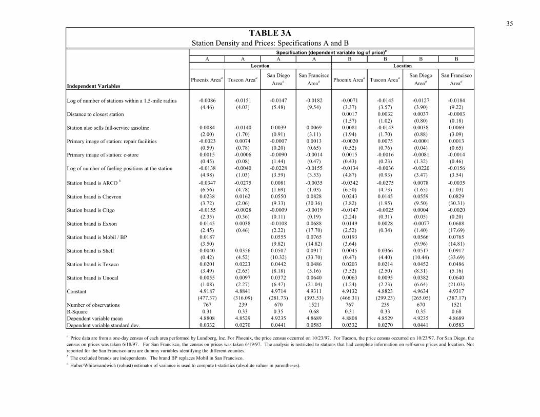
first four columns of Table 3A, denoted Specification A.19 The results provide consistent
findings regarding the relationship between seller density and average price: stations with a
greater number of competitors within a 1.5-mile radius have lower average prices. Specifically,
a 50% increase in the number of stations within a 1.5-mile radius is associated with a decrease in
the average price of approximately 0.3% in Phoenix, 0.5% in Tucson, 0.5% in San Diego, and
0.6% in San Francisco. These findings, although small in magnitude, are important in that they
provide a clear pattern in terms of the direction of change in average price accompanying a
change in seller density. In the context of the monopolistic competition models with product
differentiation, one reason why the differences are small in magnitude may be small differences
in consumers’ perceptions of variation in the desirability of gasoline from different sellers,
especially in light of the fact that we have controlled for brand differences as well as other
characteristics of the seller, such as availability of a convenience store or repair facilities. In the
context of the search models, one reason for the modest effect of market size could be low
overall search costs.
The analysis up to this point has adopted the restrictive assumption that stations are
uniformly distributed across the market. Doing so allows us to provide a simple empirical
characterization of a “market” solely by calculating the number of stations within a fixed radius.
However, Pinkse, Slade, and Brett (2002) have shown that if this were not the case, then a
second variable that could improve the characterization of the market would be the proximity of
each station’s closest competitor.20 In columns 5 through 8 of Table 3A, we provide an
19 The reported t statistics are robust to heteroscedasticity. In a supplement available at
http://www.people.virginia.edu/~sa9w/ijio/eosup.htm, we provide alternative estimates that adopt the feasible
generalized least squares (FGLS) approach. These results are similar to those reported in Table 3A.
20 Their analysis is in the context of a product differentiation model.
21
estimation of equation (4) that includes this additional variable, namely the distance to each
station's closest competitor. We refer to the modified specification of equation (4) as
specification B. Interestingly, we find no consistent, statistically significant influence of the
distance to each station’s closest competitor, although in all cases the sign of this variable's
coefficient is positive, indicating a lower expected price as the distance to a station’s closest rival
decreases, holding constant the total number of sellers in the market.
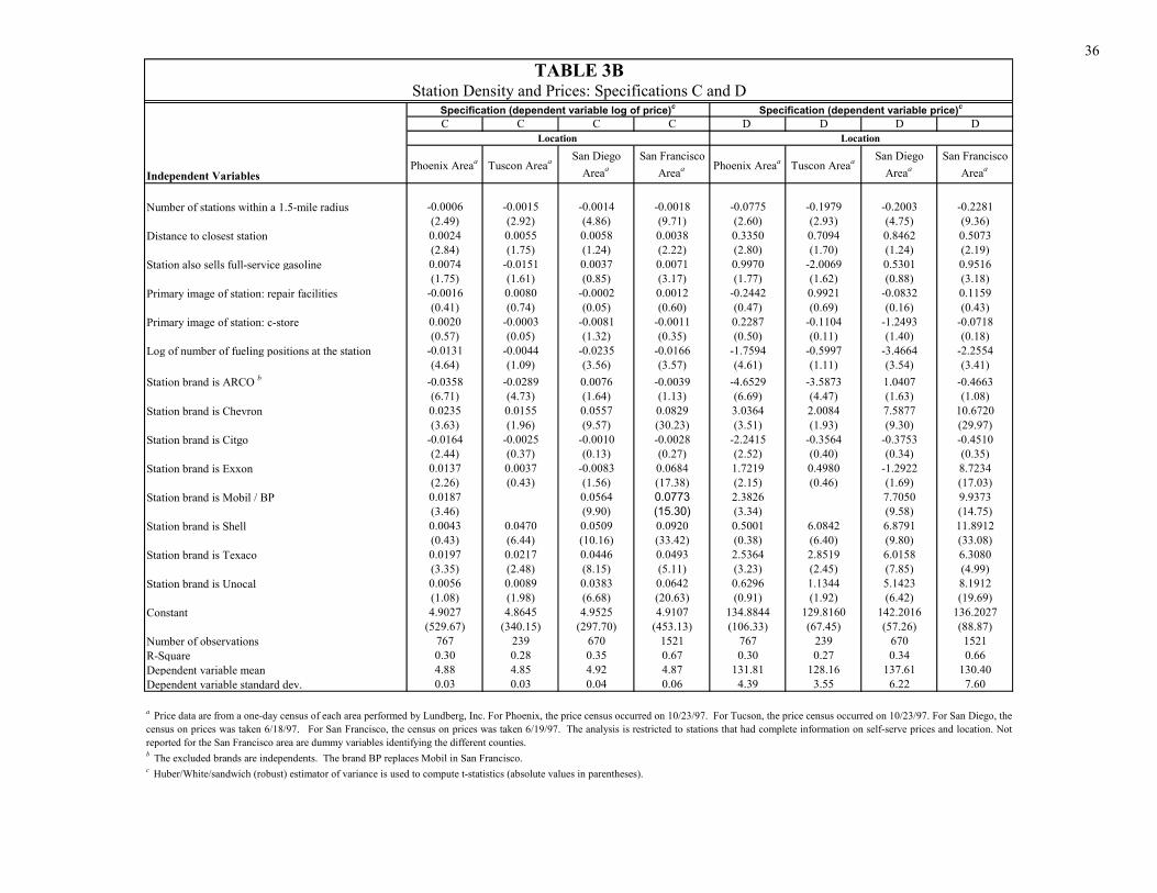
As the functional form for the predicted correlation between price and density in equation
(4) is not dictated by the theory, Table 3B presents alternative specifications to the log-log form
reported in Table 3A, specification B. In Table 3B, we refer to a new specification that uses the
number of stations within a 1.5 mile radius in levels as specification C. A new specification that
adopts measures for both the dependent variable and the number of stations within a 1.5 mile
radius in levels is denoted specification D. Two findings of interest emerge. First, our main
result of the negative effect of market density on average price holds for these alternative
specifications, suggesting that this is a robust finding. Second, for these specifications there is
evidence in three of the four market areas of a statistically significant (at the 10-percent level)
and direct relationship between price and the distance to the closest competitor station. This
result is suggested by either of the two theoretical approaches under consideration. Specifically,
for the monopolistic competition models, one expects the degree of product differentiation to be
less as competing stations are closer in distance. For the search-theoretic models, one expects a
lower search cost for consumers when competing stations are closer. Both changes suggest
lower prices as consumers become more sensitive to price changes under such circumstances.
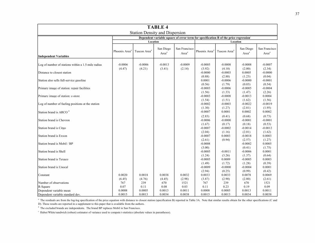
To determine the relationship between seller density and price dispersion, we estimate the
equation
( ) iii vDensityu ++= ln2 γδ , (5)
22
where are the squared residuals obtained from equation (4), and therefore measure the
unexplained variance in prices across markets. Note that this measure of price variance controls
for differences in prices that might arise due to differences in station-specific characteristics.
Equation (5) does imply that heteroscedasticity exists with respect to the estimation of (4). Thus,
in estimating (4), we adopt the Huber/White/sandwich (robust) estimator of variance to produce
consistent standard errors even when the residuals in (4) are not identically distributed.
2iu
The estimated coefficients of (5) for each of the four geographical areas is reported in the
first four columns of Table 4. The results indicate that in all four areas, an increase in the
number of stations is associated with a reduction in price dispersion as measured by the
unexplained variation in prices after controlling for station and brand attributes. These price
dispersion results are not consistent with the direct effect of an increase in the number of sellers
for either of the search-theoretic approaches discussed in Section II. As indicated by the results
in columns 5 through 8, this negative correlation between the number of stations and price
dispersion for the four markets is robust to an expanded specification of equation (5) that
includes the distance to each station’s closest competitor as well as other control variables.21
In the framework of the theoretical models presented in the previous section, an increase in
the number of sellers can be due to either an increase in market size or lower fixed costs. If it is
the former, then an increase in the number of sellers would not only be associated with lower
average prices, but also with an increase in the number of consumers per seller, as each seller
must be compensated for the lower price by an increase in total sales. Although we cannot
observe station-specific sales in our data, it is relatively easy to collect reliable information on
21 The findings reported in Table 4 are also robust to using as the dependent variable the squared error term
generated by the two alternative specifications of the price regression equation (specifications C and D) provided in
Table 3B. These findings are reported in a supplement to this paper that is available at
http://www.people.virginia.edu/~sa9w/ijio/eosup.htm.
23
the hours a station is open for business, and sellers’ weekly hours of operation have been
collected in the census surveys of stations in all four market areas.22 The increase in demand that
is predicted to accompany larger markets can increase the potential gain to a station from staying
open additional hours. We therefore expect that stations in markets with a greater number of
competitors will be open more hours. The results reported in Table 5 support this prediction. In
all four areas, the average weekly hours of operation is higher in markets with a higher density of
stations, other things equal.
At this stage, several caveats to our results are warranted. First, our results concerning
stations’ hours of operation appear consistent with the view that differences in the number of
sellers in a market reflect differences in the size of the market. However, in some instances it
may be the case that more densely populated markets are those with lower entry (fixed) costs,
suggesting that potential barriers to entry in sparsely populated markets, such as zoning
constraints, may also play a role in determining the number of sellers (station density). Note,
however, that this alternative view does not bias our predictions regarding the correlation
between station density and average price as long as barriers to entry can be interpreted in terms
of higher fixed costs and not in terms of higher marginal costs.
A second issue concerns a potential bias in our estimate of price dispersion. A key
assumption in our empirical analysis is that the underlying source of heterogeneity in prices is
invariant to the number of sellers. This means, for instance, that if we adopt the monopolistic
competition model with heterogeneous seller costs, the variance in seller costs is not related to
22 The hours of operation information was not collected during the one-day price surveys, but is taken from annual
surveys of stations performed for each area. As the status of stations can change over time, the hours data for some
stations that we have price information for are not available. In the case of the San Francisco area, the census
survey for hours covered a smaller number of counties as well. Specifically, Napa and Sonoma counties were not
included in the survey that collected information on hours.
24
market size. For the search models, this assumption implies a distribution of search costs across
consumers that is not related to market size.
IV. Discussion and Potential Extensions
The results presented in the previous section provide convincing evidence that the number
of competitors is indeed consistently linked to both price levels and price dispersion. Using
station-level data collected from every gasoline station in four large metropolitan areas, our
results indicate that a higher number of stations within a particular geographic market area is
associated with both a lower average price and a lower level of price dispersion. These results
are consistent with standard models of monopolistic competition.23 With regard to average price
levels, these findings are also consistent with the sequential-search-across-heterogeneous-sellers
approach of Carlson and McAfee (1983), but not the approach of Varian (1980) that divides the
market into informed and uninformed buyers. However, with regard to price dispersion, the
finding that an increase in the number of sellers is associated with a reduction in the variance in
prices is at odds with both search-theoretic approaches.24
The fact that our empirical findings are more in line with the monopolistic competition
models than with well-known search-theoretic models is disconcerting given that gasoline
markets appear to satisfy the key search-theoretic assumption that not all consumers know the
prices charged by all sellers. Further, in related work examining the prices of different drugs,
Sorensen (2000) finds strong support for the proposition that more frequently purchased
23 Note that with regard to the price dispersion result, our findings are at odds with the equilibrium price distribution
results for imperfectly competitive markets obtained by Dana (1999). However, the setting of the model developed
by Dana assumes capacity constraints and uncertain demand.
24 On the other hand, in support of the Varian model, Lach (2002) does find significant distribution mobility for
various food products, a finding consistent with Varian’s mixed-strategy characterization of the equilibrium price
distribution.
25
prescription drugs exhibit lower markups and less dispersion, and Sorensen attributes this
finding to the effect of lower search costs (or equivalently greater gains to search). However,
Sorensen does not formally model these predictions, and our discussion suggests that existing
search-theoretic models’ predicted effects of lower search costs on the average price and price
dispersion are not fully consistent with either our results or those of Sorensen.25 Thus,
theoretical work that modifies existing search models appears fruitful.
One example of such a modification is Anderson and Renault (1999, 2000). These authors
combine elements of search with the standard monopolistic competition model of product
differentiation. A second promising approach that retains the homogenous flavor of search-
theoretic models is suggested by Anderson and de Palma (2002). This paper is attractive in that
it relaxes the strong assumption made by standard search-theoretic models that consumers know
the distribution of prices, an assumption that requires a seller, in setting its price, to anticipate
consumers’ reservation price reactions to a price change. Instead, Anderson and de Palma
introduce a given distribution of reservation prices among consumers. They then show that one
can generate equilibrium price dispersion in such a model without adopting Carlson and
McAfee’s assumption of heterogeneity in sellers’ costs. Further, Anderson and de Palma obtain
the result that an increase in the number of sellers can reduce the average price, although these
results are partial in nature as their analysis takes the number of sellers to be exogenous.
Anderson and de Palma (2002) take an important step toward relaxing the strong assumption
of standard sequential search models that buyers have full knowledge of the distribution of prices
but no knowledge of the location of individual prices across sellers. Another approach that
25 Recall that while both the Carlson and McAfee or the Varian-type models predict reduced search costs will lower
the average price, lower search costs are predicted to either increase the variance of prices or to have an ambiguous
effect on the variance.
26
would directly address this issue of the appropriate information set for buyers would be to
consider each buyer as acquiring imperfect signals regarding the prices at each seller i given by
ηαεα )1()( −++−+= ppps ii , (6)
where ε and η are random variables with mean zero, respective finite variances and ,
and uncorrelated across buyers and sellers. In the standard search-theoretic model, α = 0, is
the variance of the price distribution, and the signal is not informative. But in many markets,
gasoline and prescription drugs being two examples, the idea that individuals may have some
information on the prices charged by different sellers either from past purchases or from seller
advertising is appealing.
2εσ
2ησ
2ησ
Consider the case when α = 1. In such a setting, each buyer would initially visit the seller
that, according to the signals received, is thought to have the lowest price. Buyers would then
have the option of incurring a search cost, c, to visit another seller if the actual price turned out
to be sufficiently high to create a gain to further search. In this context, there are three
parameters that can affect the responsiveness of demand to a change in price. The first is the
quality of information customers have concerning alternatives, which is measured by the
precision of price signals, εσ/1 . The second is the cost to consumers of seeking out an
alternative seller, which is measured by the search cost parameter, c. The third is the number of
sellers, as this determines the likelihood that a buyer will perceive a gain to visiting another
seller.
In such a model, one can show that if prices were identical across sellers, then more precise
signals, lower search costs, or a larger number of sellers increases the responsiveness of quantity
demanded to a change in price for each seller. Further, if one were to assume that firms also
obtain imperfect signals each period as to the prices charged by other sellers in the market, one
can generate not only an equilibrium distribution of prices, but also the comparative static result
27
that lower search costs or an increase in the number of sellers reduces the mean price and the
variance in prices, a result consistent with our empirical findings.
28
Acknowledgements
A portion of Beck Taylor’s work was completed while a visiting scholar at Harvard University.
The authors thank Simon Anderson, two anonymous referees, and seminar participants at
University of Oregon for very helpful comments on earlier drafts. Of course, we retain
responsibility for any errors.
29
References
Abbott III, Thomas A., 1994, Observed price dispersion: Product heterogeneity, regional
markets, or local market power? Journal of Economics and Business 46, 21-37.
Adams III, A.F., 1997, Search costs and price dispersion in a localized, homogeneous product
market: Some empirical evidence, Review of Industrial Organization 12, 801-808.
Agarwal, V.B. and R.T. Deacon, 1985, Price controls, price dispersion and the supply of refined
petroleum products, Energy Economics 7, 210-219.
Anderson, S.P. and A. de Palma, 2001, Product diversity in asymmetric oligopoly: Is the quality
of consumer goods too low? The Journal of Industrial Economics 49, 113-135.
_____, 2002, Price dispersion, working paper.
Anderson, S.P., A. de Palma, and Y. Nesterov, 1995, Oligopolistic competition and the optimal
provision of products, Econometrica 63, 1281-1301.
Anderson, S.P. and R. Renault, 1999, Pricing, product diversity, and search costs: A Bertrand-
Chamberlin-Diamond model, RAND Journal of Economics 30, 719-735.
_____, 2000, Consumer information and pricing: Negative externalities from improved
information, International Economic Review 41, 721-742.
Barron, J.M., B.A. Taylor, and J.R. Umbeck, 2000, A theory of quality-related differences in
retail margins: Why there is a ‘premium’ on premium gasoline, Economic Inquiry 38,
550-569.
Borenstein, S. and N.L. Rose, 1994, Competition and price dispersion in the US airline industry,
Journal of Political Economy 102, 653-683.
Burdett, K. and K.L. Judd, 1983, Equilibrium price dispersion, Econometrica 51, 955-969.
Carlson, J.A. and R.P. McAfee, 1982, Discrete equilibrium price dispersion: Extensions and
technical details, Institute Paper no. 812, Purdue University.
30
_____, 1983, Discrete equilibrium price dispersion, Journal of Political Economy 91, 480-493.
Cohen, M., 1998, Linking price dispersion to product differentiation – Incorporating aspects of
consumer involvement, Applied Economics 30, 829-835.
Dahlby, B. and D.S. West, 1986, Price dispersion in an automobile insurance market, Journal of
Political Economy 94, 418-438.
Dana, J.D., 1999, Equilibrium price dispersion under demand uncertainty: The roles of costly
capacity and market structure, RAND Journal of Economics 30, 632-660.
Giulietti, M. and M. Waterson, 1997, Multiproduct firms’ pricing behaviour in the Italian
grocery trade, Review of Industrial Organization 12, 817-832.
Guimãraes, P., 1996, Search intensity in oligopoly, Journal of Industrial Economics 44, 415-
426.
Hayes, K.J. and L.B. Ross, 1998, Is airline price dispersion the result of careful planning or
competitive forces? Review of Industrial Organization 13, 523-541.
Hogan, S.D., 1991, The inefficiency of arbitrage in an equilibrium-search model, Review of
Economic Studies 58, 755-775.
Lach, S., 2002, Existence and persistence of price dispersion: An empirical analysis, Review of
Economics and Statistics 84, 433-444.
Marvel, H.P., 1976, The economics of information and retail gasoline price behavior: An
empirical analysis, Journal of Political Economy 84, 1033-1060.
Perloff, J.M. and S.C. Salop, 1985, Equilibrium with product differentiation, The Review of
Economic Studies 52, 107-120.
Pinkse, J., M.E. Slade, and C. Brett, 2002, Spatial price competition: A semiparametic approach,
Econometrica 70, 1111-1153.
Pratt, J.W., D.A. Wise, and R.J. Zeckhauser, 1979, Price differences in almost competitive
markets, Quarterly Journal of Economics 92, 189-211.
31
Png, I.P.L. and D. Reitman, 1994, Service time competition, RAND Journal of Economics 25,
619-634.
Reinganum, J., 1979, A simple model of equilibrium price dispersion, Journal of Political
Economy 87, 851-858.
Rosenthal, R.W., 1980, A model in which an increase in the number of sellers leads to a higher
price, Econometrica 48, 1575-1579.
Samuelson, L. and J. Zhang, 1992, Search costs and prices, Economics Letters 38, 55-60.
Schmidt, S., 2001, Market structure and market outcomes in deregulated rail freight markets,
International Journal of Industrial Organization 19, 99-131.
Shepard, A., 1991, Price discrimination and retail configuration, Journal of Political Economy
99, 30-53.
Sorensen, A.T., 2000, Equilibrium price dispersion in retail markets for prescription drugs,
Journal of Political Economy 108, 833-850.
Stahl, D.O., 1989, Oligopolistic pricing with sequential consumer search, American Economic
Review 79, 700-712.
______, 1996, Oligopolistic pricing with heterogeneous consumer search, International Journal
of Industrial Organization 14, 243-268.
Stiglitz, J.E., 1987, Competition and the number of firms in a market: Are duopolies more
competitive than atomistic markets, Journal of Political Economy 95, 1041-1061.
Van Hoomissen, T., 1988, Price dispersion and inflation: Evidence from Israel, Journal of
Political Economy 96, 1303-1314.
Varian, H.R., 1980, A model of sales, American Economic Review 70, 651-659.
Villas-Boas, J.M., 1995, Models of competitive price promotions: Some empirical evidence from
the coffee and saltine crackers markets, Journal of Economics and Management Strategy
4, 85-107.
32
Walsh, P.R. and C. Whelan, 1999, Modeling price dispersion as an outcome of competition in
the Irish grocery market, Journal of Industrial Economics 47, 325-343.
33
Number of sellers and
average price
Number of sellers and price
dispersion
Range of visiting or search costs
and average price
Range of visiting or search costs
and price dispersion
Product-differentiation model with heterogeneity in sellers' demands or heterogeneity in sellers' costs
negative negative positive positive
Search-theoretic model with heterogeneity in consumers' search costs and sellers' costs (Carlson and McAfee, 1983)
negative positive positive uncorrelated
Search-theoretic model with heterogeneity in consumers' search costs (Varian, 1980)
positive positive positive ambiguous
Predicted Correlations Between:
TABLE 1Summary of Predicted Correlations*
Model of equilibrium price distribution:
*Recall that for the Varian-type model, a reduced range of search costs is interpreted as an increase in the proportion of consumers that are informed. The results reported above reflect the correlations suggested by changes in market size or entry costs that alter both the number of sellers in a market and the equilibrium prices in the context of different search models. The results for the product differentition models are reasonable extensions of results for the homogeneous case. The results for Carlson and McAfee are reported in their paper, and reflect, among other factors, a specific distributional assumption on search costs. The Varian results are generated using a specific example provided by Varian.
34
Phoenix Areaa Tuscon Areaa San Diego Areaa San Francisco Areaa
Price at station (regular unleaded self-serve) 131.9 128.2 137.7 130.4(4.39) (3.56) (6.22) (7.61)
Weekly hours of operation 154.84 155 150.14 144.75(32.93) (27.71) (31.23) (28.3)
Number of stations within a 1.5-mile radius 9.38 8.34 8.59 10.58(5.16) (4.47) (5.86) (5.84)
Distance to closest station 0.48 0.33 0.36 0.28(1.66) (0.57) (0.92) (0.62)
Station also sells full-service gasoline 0.11 0.14 0.15 0.17(0.31) (0.35) (0.35) (0.38)
Primary image of station: repair facilities 0.18 0.18 0.34 0.44(0.38) (0.38) (0.48) (0.5)
Primary image of station: c-store 0.54 0.61 0.3 0.17(0.5) (0.49) (0.46) (0.37)
Number of fueling positions at the station 7.88 6.8 7.41 7.56(3.96) (3.44) (2.98) (2.64)
Station brand is ARCO b 0.1 0.06 0.15 0.09(0.3) (0.23) (0.36) (0.28)
Station brand is Chevron 0.07 0.13 0.12 0.18(0.26) (0.34) (0.32) (0.39)
Station brand is Citgo 0.05 0.03 0.1 0.01(0.21) (0.17) (0.3) (0.1)
Station brand is Exxon 0.09 0.08 0.01 0.07(0.28) (0.26) (0.04) (0.26)
Station brand is Mobil / BP 0.15 0.1 0.04(0.36) (0.3) (0.19)
Station brand is Shell 0.03 0.01 0.14 0.2(0.15) (0.07) (0.35) (0.4)
Station brand is Texaco 0.13 0.16 0.11 0.02(0.34) (0.36) (0.31) (0.11)
Station brand is Unocal 0.31 0.39 0.1 0.17(0.47) (0.49) (0.3) (0.38)
Number of observations 767 239 670 1521
TABLE 2Descriptive Statistics for Four Areas
Descriptive Statistics: Mean (standard error)
b The excluded brands are independents. The brand BP replaces Mobil in San Francisco.
Variables
a Price data are from a one-day census of each area performed by Lundberg, Inc. For Phoenix, the price census occurred on 10/23/97. For Tucson, the price censusoccurred on 10/23/97. For San Diego, the census on prices was taken 6/18/97. For San Francisco, the census on prices was taken 6/19/97. The analysis is restrictedto stations that had complete information on self-serve prices, hours, and location.
35
A A A A B B B B
Phoenix Areaa Tuscon Areaa San Diego Areaa
San Francisco Areaa Phoenix Areaa Tuscon Areaa San Diego
AreaaSan Francisco
Areaa
Log of number of stations within a 1.5-mile radius -0.0086 -0.0151 -0.0147 -0.0182 -0.0071 -0.0145 -0.0127 -0.0184(4.46) (4.03) (5.48) (9.54) (3.37) (3.57) (3.90) (9.22)
Distance to closest station 0.0017 0.0032 0.0037 -0.0003(1.57) (1.02) (0.80) (0.18)
Station also sells full-service gasoline 0.0084 -0.0140 0.0039 0.0069 0.0081 -0.0143 0.0038 0.0069(2.00) (1.70) (0.91) (3.11) (1.94) (1.70) (0.88) (3.09)
Primary image of station: repair facilities -0.0023 0.0074 -0.0007 0.0013 -0.0020 0.0075 -0.0001 0.0013(0.59) (0.78) (0.20) (0.65) (0.52) (0.76) (0.04) (0.65)
Primary image of station: c-store 0.0015 -0.0006 -0.0090 -0.0014 0.0015 -0.0016 -0.0081 -0.0014(0.45) (0.08) (1.44) (0.47) (0.43) (0.23) (1.32) (0.46)
Log of number of fueling positions at the station -0.0138 -0.0040 -0.0228 -0.0155 -0.0134 -0.0036 -0.0220 -0.0156(4.98) (1.03) (3.59) (3.53) (4.87) (0.93) (3.47) (3.54)
Station brand is ARCO b -0.0347 -0.0275 0.0081 -0.0035 -0.0342 -0.0275 0.0078 -0.0035(6.56) (4.78) (1.69) (1.03) (6.50) (4.73) (1.65) (1.03)
Station brand is Chevron 0.0238 0.0162 0.0550 0.0828 0.0243 0.0145 0.0559 0.0829(3.72) (2.06) (9.33) (30.36) (3.82) (1.95) (9.50) (30.31)
Station brand is Citgo -0.0155 -0.0028 -0.0009 -0.0019 -0.0147 -0.0025 0.0004 -0.0020(2.35) (0.36) (0.11) (0.19) (2.24) (0.31) (0.05) (0.20)
Station brand is Exxon 0.0145 0.0038 -0.0108 0.0688 0.0149 0.0028 -0.0077 0.0688(2.45) (0.46) (2.22) (17.70) (2.52) (0.34) (1.40) (17.69)
Station brand is Mobil / BP 0.0187 0.0555 0.0765 0.0193 0.0566 0.0765(3.50) (9.82) (14.82) (3.64) (9.96) (14.81)
Station brand is Shell 0.0040 0.0356 0.0507 0.0917 0.0045 0.0366 0.0517 0.0917(0.42) (4.52) (10.32) (33.70) (0.47) (4.40) (10.44) (33.69)
Station brand is Texaco 0.0201 0.0223 0.0442 0.0486 0.0203 0.0214 0.0452 0.0486(3.49) (2.65) (8.18) (5.16) (3.52) (2.50) (8.31) (5.16)
Station brand is Unocal 0.0055 0.0097 0.0372 0.0640 0.0063 0.0095 0.0382 0.0640(1.08) (2.27) (6.47) (21.04) (1.24) (2.23) (6.64) (21.03)
Constant 4.9187 4.8841 4.9714 4.9311 4.9132 4.8823 4.9634 4.9317(477.37) (316.09) (281.73) (393.53) (466.31) (299.23) (265.05) (387.17)
Number of observations 767 239 670 1521 767 239 670 1521R-Square 0.31 0.33 0.35 0.68 0.31 0.33 0.35 0.68Dependent variable mean 4.8808 4.8529 4.9235 4.8689 4.8808 4.8529 4.9235 4.8689Dependent variable standard dev. 0.0332 0.0270 0.0441 0.0583 0.0332 0.0270 0.0441 0.0583
c Huber/White/sandwich (robust) estimator of variance is used to compute t-statistics (absolute values in parentheses).
a Price data are from a one-day census of each area performed by Lundberg, Inc. For Phoenix, the price census occurred on 10/23/97. For Tucson, the price census occurred on 10/23/97. For San Diego, thecensus on prices was taken 6/18/97. For San Francisco, the census on prices was taken 6/19/97. The analysis is restricted to stations that had complete information on self-serve prices and location. Notreported for the San Francisco area are dummy variables identifying the different counties. b The excluded brands are independents. The brand BP replaces Mobil in San Francisco.
TABLE 3AStation Density and Prices: Specifications A and B
Independent Variables
Location Location
Specification (dependent variable log of price)c
36
C C C C D D D D
Phoenix Areaa Tuscon Areaa San Diego Areaa
San Francisco Areaa Phoenix Areaa Tuscon Areaa San Diego
AreaaSan Francisco
Areaa
Number of stations within a 1.5-mile radius -0.0006 -0.0015 -0.0014 -0.0018 -0.0775 -0.1979 -0.2003 -0.2281(2.49) (2.92) (4.86) (9.71) (2.60) (2.93) (4.75) (9.36)
Distance to closest station 0.0024 0.0055 0.0058 0.0038 0.3350 0.7094 0.8462 0.5073(2.84) (1.75) (1.24) (2.22) (2.80) (1.70) (1.24) (2.19)
Station also sells full-service gasoline 0.0074 -0.0151 0.0037 0.0071 0.9970 -2.0069 0.5301 0.9516(1.75) (1.61) (0.85) (3.17) (1.77) (1.62) (0.88) (3.18)
Primary image of station: repair facilities -0.0016 0.0080 -0.0002 0.0012 -0.2442 0.9921 -0.0832 0.1159(0.41) (0.74) (0.05) (0.60) (0.47) (0.69) (0.16) (0.43)
Primary image of station: c-store 0.0020 -0.0003 -0.0081 -0.0011 0.2287 -0.1104 -1.2493 -0.0718(0.57) (0.05) (1.32) (0.35) (0.50) (0.11) (1.40) (0.18)
Log of number of fueling positions at the station -0.0131 -0.0044 -0.0235 -0.0166 -1.7594 -0.5997 -3.4664 -2.2554(4.64) (1.09) (3.56) (3.57) (4.61) (1.11) (3.54) (3.41)
Station brand is ARCO b -0.0358 -0.0289 0.0076 -0.0039 -4.6529 -3.5873 1.0407 -0.4663(6.71) (4.73) (1.64) (1.13) (6.69) (4.47) (1.63) (1.08)
Station brand is Chevron 0.0235 0.0155 0.0557 0.0829 3.0364 2.0084 7.5877 10.6720(3.63) (1.96) (9.57) (30.23) (3.51) (1.93) (9.30) (29.97)
Station brand is Citgo -0.0164 -0.0025 -0.0010 -0.0028 -2.2415 -0.3564 -0.3753 -0.4510(2.44) (0.37) (0.13) (0.27) (2.52) (0.40) (0.34) (0.35)
Station brand is Exxon 0.0137 0.0037 -0.0083 0.0684 1.7219 0.4980 -1.2922 8.7234(2.26) (0.43) (1.56) (17.38) (2.15) (0.46) (1.69) (17.03)
Station brand is Mobil / BP 0.0187 0.0564 0.0773 2.3826 7.7050 9.9373(3.46) (9.90) (15.30) (3.34) (9.58) (14.75)
Station brand is Shell 0.0043 0.0470 0.0509 0.0920 0.5001 6.0842 6.8791 11.8912(0.43) (6.44) (10.16) (33.42) (0.38) (6.40) (9.80) (33.08)
Station brand is Texaco 0.0197 0.0217 0.0446 0.0493 2.5364 2.8519 6.0158 6.3080(3.35) (2.48) (8.15) (5.11) (3.23) (2.45) (7.85) (4.99)
Station brand is Unocal 0.0056 0.0089 0.0383 0.0642 0.6296 1.1344 5.1423 8.1912(1.08) (1.98) (6.68) (20.63) (0.91) (1.92) (6.42) (19.69)
Constant 4.9027 4.8645 4.9525 4.9107 134.8844 129.8160 142.2016 136.2027(529.67) (340.15) (297.70) (453.13) (106.33) (67.45) (57.26) (88.87)
Number of observations 767 239 670 1521 767 239 670 1521R-Square 0.30 0.28 0.35 0.67 0.30 0.27 0.34 0.66Dependent variable mean 4.88 4.85 4.92 4.87 131.81 128.16 137.61 130.40Dependent variable standard dev. 0.03 0.03 0.04 0.06 4.39 3.55 6.22 7.60
Independent Variables
Specification (dependent variable price)cSpecification (dependent variable log of price)c
TABLE 3BStation Density and Prices: Specifications C and D
Location Location
c Huber/White/sandwich (robust) estimator of variance is used to compute t-statistics (absolute values in parentheses).
a Price data are from a one-day census of each area performed by Lundberg, Inc. For Phoenix, the price census occurred on 10/23/97. For Tucson, the price census occurred on 10/23/97. For San Diego, thecensus on prices was taken 6/18/97. For San Francisco, the census on prices was taken 6/19/97. The analysis is restricted to stations that had complete information on self-serve prices and location. Notreported for the San Francisco area are dummy variables identifying the different counties. b The excluded brands are independents. The brand BP replaces Mobil in San Francisco.
37
Phoenix Areaa Tuscon Areaa San Diego Areaa
San Francisco Areaa Phoenix Areaa Tuscon Areaa San Diego
AreaaSan Francisco
Areaa
Log of number of stations within a 1.5-mile radius -0.0006 -0.0006 -0.0013 -0.0009 -0.0005 -0.0008 -0.0008 -0.0007(4.47) (4.21) (3.41) (2.14) (3.92) (4.10) (2.00) (2.34)
Distance to closest station -0.0000 -0.0003 0.0005 -0.0000(0.88) (2.88) (1.23) (0.04)
Station also sells full-service gasoline 0.0001 -0.0006 -0.0000 -0.0001(0.56) (1.79) (0.03) (0.54)
Primary image of station: repair facilities -0.0003 -0.0006 -0.0005 -0.0004(1.56) (1.33) (1.47) (2.26)
Primary image of station: c-store -0.0003 -0.0008 -0.0013 0.0004(1.54) (1.51) (1.62) (1.56)
Log of number of fueling positions at the station -0.0002 -0.0003 -0.0022 -0.0019(1.30) (1.27) (2.81) (1.95)
Station brand is ARCO b -0.0007 0.0001 0.0002 0.0002(2.83) (0.41) (0.68) (0.73)
Station brand is Chevron -0.0006 -0.0000 -0.0001 -0.0001(1.67) (0.17) (0.18) (0.53)
Station brand is Citgo -0.0007 -0.0002 -0.0014 -0.0012(2.04) (1.16) (2.01) (1.62)
Station brand is Exxon -0.0007 0.0003 -0.0018 0.0003(2.61) (0.94) (2.57) (1.27)
Station brand is Mobil / BP -0.0008 -0.0002 0.0005(3.00) (0.41) (1.75)
Station brand is Shell -0.0005 -0.0011 -0.0006 0.0001(1.24) (3.26) (1.37) (0.64)
Station brand is Texaco -0.0005 0.0009 -0.0005 0.0003(1.49) (1.72) (1.28) (0.39)
Station brand is Unocal -0.0009 -0.0000 -0.0004 0.0001(2.94) (0.25) (0.99) (0.42)
Constant 0.0020 0.0018 0.0038 0.0032 0.0033 0.0033 0.0078 0.0069(6.45) (4.76) (4.45) (2.98) (3.87) (2.90) (2.80) (2.61)
Number of observations 767 239 670 1521 767 239 670 1521R-Square 0.07 0.11 0.08 0.03 0.11 0.23 0.19 0.09Dependent variable mean 0.0008 0.0005 0.0013 0.0011 0.0008 0.0005 0.0013 0.0011Dependent variable standard dev. 0.0015 0.0013 0.0034 0.0038 0.0015 0.0013 0.0034 0.0038
Location
TABLE 4Station Density and Dispersion
Dependent variable square of error term for specification B of the price regressionc
Independent Variables
Location
a The residuals are from the log-log specification of the price equation with distance to closest station (specification B) reported in Table 3A. Note that similar results obtain for the other specifications (C andD). These results are reported in a supplement to this paper that is available from the authors.b The excluded brands are independents. The brand BP replaces Mobil in San Francisco.c Huber/White/sandwich (robust) estimator of variance used to compute t-statistics (absolute values in parentheses).
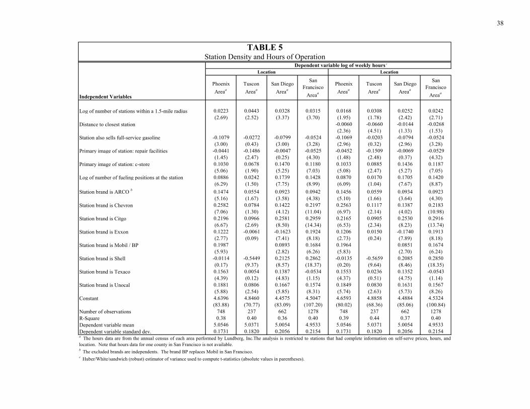
38
Phoenix Areaa
Tuscon Areaa
San Diego Areaa
San Francisco
Areaa
Phoenix Areaa
Tuscon Areaa
San Diego Areaa
San Francisco
Areaa
Log of number of stations within a 1.5-mile radius 0.0223 0.0443 0.0328 0.0315 0.0168 0.0308 0.0252 0.0242(2.69) (2.52) (3.37) (3.70) (1.95) (1.78) (2.42) (2.71)
Distance to closest station -0.0060 -0.0660 -0.0144 -0.0268(2.36) (4.51) (1.33) (1.53)
Station also sells full-service gasoline -0.1079 -0.0272 -0.0799 -0.0524 -0.1069 -0.0203 -0.0794 -0.0524(3.00) (0.43) (3.00) (3.28) (2.96) (0.32) (2.96) (3.28)
Primary image of station: repair facilities -0.0441 -0.1486 -0.0047 -0.0525 -0.0452 -0.1509 -0.0069 -0.0529(1.45) (2.47) (0.25) (4.30) (1.48) (2.48) (0.37) (4.32)
Primary image of station: c-store 0.1030 0.0678 0.1470 0.1180 0.1033 0.0885 0.1436 0.1187(5.06) (1.90) (5.25) (7.03) (5.08) (2.47) (5.27) (7.05)
Log of number of fueling positions at the station 0.0886 0.0242 0.1739 0.1428 0.0870 0.0170 0.1705 0.1420(6.29) (1.50) (7.75) (8.99) (6.09) (1.04) (7.67) (8.87)
Station brand is ARCO b 0.1474 0.0554 0.0923 0.0942 0.1456 0.0559 0.0934 0.0923(5.16) (1.67) (3.58) (4.38) (5.10) (1.66) (3.64) (4.30)
Station brand is Chevron 0.2582 0.0784 0.1422 0.2197 0.2563 0.1117 0.1387 0.2183(7.06) (1.30) (4.12) (11.04) (6.97) (2.14) (4.02) (10.98)
Station brand is Citgo 0.2196 0.0966 0.2581 0.2959 0.2165 0.0905 0.2530 0.2916(6.67) (2.69) (8.50) (14.34) (6.53) (2.34) (8.23) (13.74)
Station brand is Exxon 0.1222 -0.0061 -0.1623 0.1924 0.1206 0.0150 -0.1740 0.1913(2.77) (0.09) (7.41) (8.18) (2.73) (0.24) (7.89) (8.18)
Station brand is Mobil / BP 0.1987 0.0893 0.1684 0.1964 0.0851 0.1674(5.93) (2.82) (6.26) (5.83) (2.70) (6.24)
Station brand is Shell -0.0114 -0.5449 0.2125 0.2862 -0.0135 -0.5659 0.2085 0.2850(0.17) (9.37) (8.57) (18.37) (0.20) (9.64) (8.46) (18.35)
Station brand is Texaco 0.1563 0.0054 0.1387 -0.0534 0.1553 0.0236 0.1352 -0.0543(4.39) (0.12) (4.83) (1.15) (4.37) (0.51) (4.75) (1.14)
Station brand is Unocal 0.1881 0.0806 0.1667 0.1574 0.1849 0.0830 0.1631 0.1567(5.88) (2.54) (5.85) (8.31) (5.74) (2.63) (5.73) (8.26)
Constant 4.6396 4.8460 4.4575 4.5047 4.6593 4.8858 4.4884 4.5324(83.88) (70.77) (83.09) (107.20) (80.02) (68.36) (85.06) (100.84)
Number of observations 748 237 662 1278 748 237 662 1278R-Square 0.38 0.40 0.36 0.40 0.39 0.44 0.37 0.40Dependent variable mean 5.0546 5.0371 5.0054 4.9533 5.0546 5.0371 5.0054 4.9533Dependent variable standard dev. 0.1731 0.1820 0.2056 0.2154 0.1731 0.1820 0.2056 0.2154
Dependent variable log of weekly hours c
Independent Variables
TABLE 5Station Density and Hours of Operation
c Huber/White/sandwich (robust) estimator of variance used to compute t-statistics (absolute values in parentheses).
a The hours data are from the annual census of each area performed by Lundberg, Inc.The analysis is restricted to stations that had complete information on self-serve prices, hours, andlocation. Note that hours data for one county in San Francisco is not available.b The excluded brands are independents. The brand BP replaces Mobil in San Francisco.
Location Location