P R E V I O U S L Y I S S U E D N U M B E R S O F B R U E L & K J / E R T E C H N I C A L R E V I E W

1 1975 Problems in Telephone Measurements. Proposals for the Measurement of Loudness Ratings of Operators' Headsets. Comparison of Results obtained by Subjective Measuring Methods. Repeatabilities in Electro-Acoustic Measurements on Telephone Capsules. Stable Subset Measurements with the 73 D Vibration Testing of Telephone Equipment.

4 1974 Underwater Impulse Measurements, A Comparison of ISO and OSHA Noise Dose Measurements. Sound Radiation from Loudspeaker System with the Symmetry of the Platonic Solids.

3 1974 Acoustical Investigation of an Impact Drill. Measurement of the Dynamic Mass of the Hand-arm System.

2-1974 On Signal/Noise Ratio of Tape Recorders. On the Operating Performance of the Tape Recorder Type 7003 in a Vibrating Environment.

1-1974 Measurements of averaging times of Levet Recorders Types 2305 and 2307, A simple Equipment for direct Measurement of Reverbe­ration Time using Level Recorder Type 2305. Influence of Sunbeams striking the Diaphragms of Mea­suring Microphones.

4 1973 Laboratory tests of the Dynamic Performance of a Turbocharger Rotor-Bearing System, Measurements on the Resonance Frequencies of a Turbocharger Rotor.

3 1973 Sources of Error in Noise Dose Measurements. Infrasonic Measurements. Determination of Resonance Frequencies of Blades and Disc of a Compressor Impeller.

2 1973 High Speed Narrow Band Analysis using the Digital Event Recorder Type 7502. Calibration Problems in Bone Vibration with reference to IEC R373 and ANSI S3. 13-1972. An Investigation of the Near Field Screen Efficiency for Noise Attenuation.

(Continued on cover page 3)

TECHNICAL REVIEW

No. 2 — 1975

Contents

On the Averaging Time of RMS Measurements by C. G. Wahrmann and J . T. Broch 3

Averaging Time of Level Recorder Type 2 3 0 6 and " F a s t " and " S l o w " Response of Level Recorders 2 3 0 5 / 0 6 / 0 7

by K. Zaveri 22

N ews f rom the Factory 39

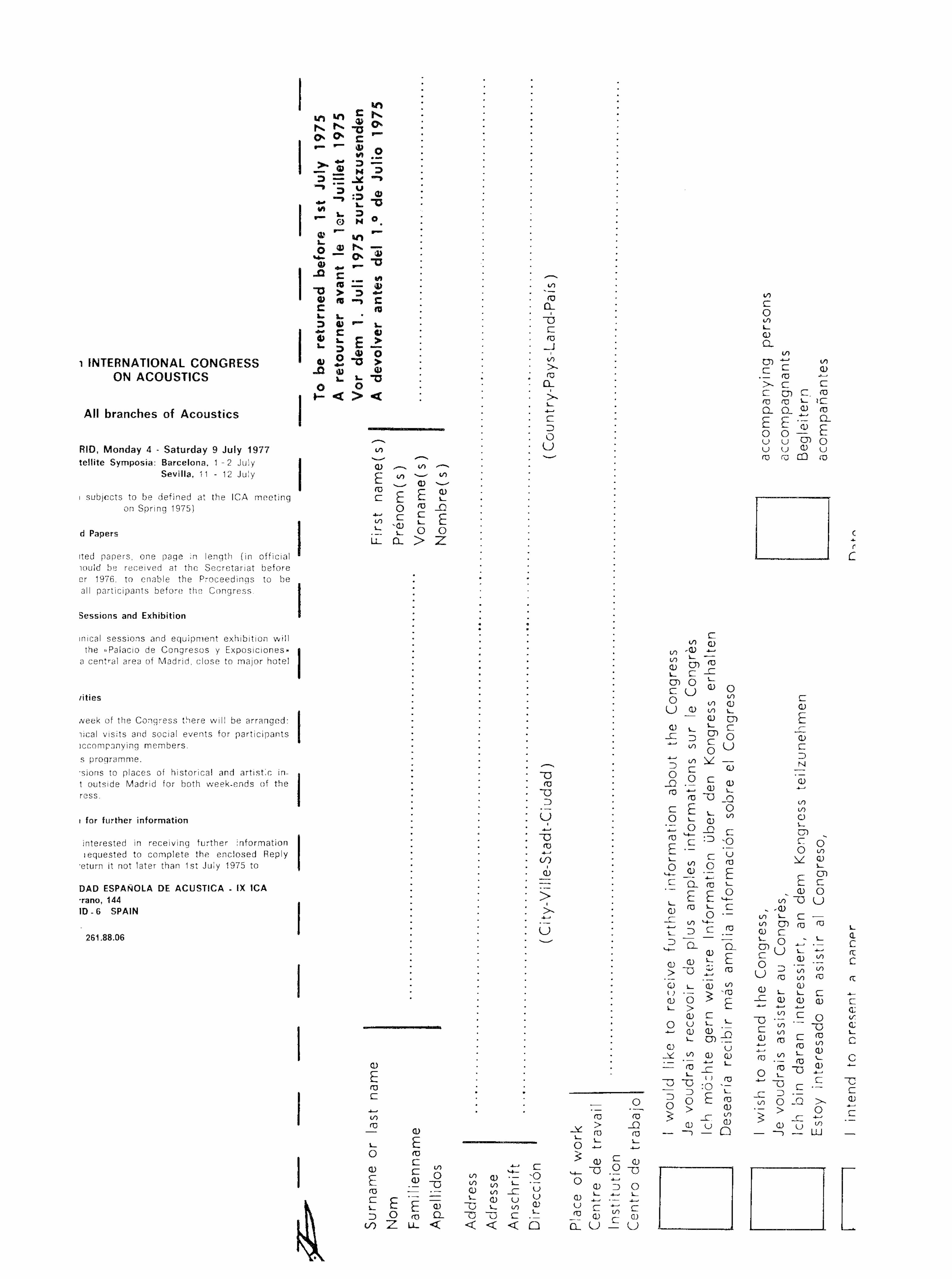
Announcement for the 9th International Congress on Acoust ics 43

On the Averaging Time of RMS Measurements

by

C. G. Wahrmann and J. T. Broch

ABSTRACT

Time averaging and /o r weight ing are some of the most important processes in data reduc­t ion measurement systems. This paper deals w i th these processes as applied to RMS (Or MS) measurements. After intro­ducing various kinds of t ime averaging techniques, the t ime and frequency domain descrip­tions of averaging processes are briefly out l ined, part icularly w i th regard to the most import­ant practical averaging systems: The running integration technique and the RC-weight ing technique. Comparing the use of these two techniques in the measurement of stationary random signals the important "equivalence cr i te r ion" T = 2 RC is derived. This result is then applied to the measurement of stationary periodic signals, and it is shown that also in these cases T = 2 RC is a satisfactory practical "equivalence cr i te r ion" .

The paper wi l l be extended in the next issue of the B & K Technical Review, where the differ­ent kinds of integrat ion/averaging techniques are applied to transient and impulsive sig­nals, and some general conclusions are formulated.

SOMMAIRE L'integration et (ou) la ponderation temporelles sont parmi les processus les plus importants pour la reduction des resultats dans les systemes de mesure.

Cet article traite de ces processus appliques aux mesures de valeur efficace (ou de moyenne quadratique). Apres I n t r oduc t i on de differentes techniques d' integrat ion temporel le, les des­cript ions, dans les domaines du temps et des frequences, des procedures d' integrat ion sont rapidements etudiees, en prenant part icul ierement en consideration les plus importants des systemes pratiques: l ' integration cont inue et la ponderation RC. En comparant I'emploi de ces deux techniques pour les mesures sur des signaux aleatoires stat ionnaires, on abouti a I ' important "cr i tere d 'equivalence" T - 2 RC.

Ce resuitat est ensuite applique a la mesure de signaux periodiques stat ionnaires, et Ton montre que, dans ce cas, la relation T ~ 2 RC est aussi un "cr i tere d 'equivalence" pratique satisfaisant.

Cet article sera complete dans la prochaine edit ion de la Revue Technique B & K, ou les diffe­rentes techniques d' integrat ion et de ponderation seront appliquees aux signaux transitoires et impulsionnels et ou certaines conclusions generaies seront t irees.

3

ZUSAMMENFASSUNG Die zeitl iche Mi t te lung mit und ohne zeitabhangige Bewertung ist einer der wicht igsten Pro-zesse in datenreduzierenden Mef tsystemen.

Dieser Beitrag beschreibt solche Prozesse, angewandt auf den Effektivwert (oder quadrat i -schen Mi t te lwert ) . Nach einer Einfuhrung in verschiedene Arten von Zeitmit t lungs — Techni-ken w i rd die Darstel lung von Mitt lungsprozessen im Zeit — wie im Frequenzraum kurz aufge-zeigt, insbesondere im Hinblick auf die praktisch bedeutsamsten Mit t lungsarten: die Technik der gleitenden Integration und der RC-Mit t !ung. Durch Vergleich dieser beiden Techniken in

j ■

Anwendung auf die Messung stationarer stochastischer Signale w i rd das wicht ige "Aquiva-lenskr i ter ium" T = 2 RC hergeleitet.

Dies Ergebnis w i rd dann angewandt auf die Messung stationarer periodischer Signale, und es zeigt sich, daft auch in diesem Fall T = 2 RC ein fur die Praxis zufr iedenstel lendes Krite-r ium darstellt.

Der Art ikel w i rd in der nachsten Ausgabe der B & K Technical Review fortgesetzt, wobei die verschiedenen Arten von In tegrat ionsVMi t t lungstechniken auf f lucht ige und impulsart ige Si­gnale angewandt und einige al lgemeine Schluf t fo lgerungen formul iert werden.

1 . Introduction The most complete description of a signal is obtained by recording its entire time history. This is, however, not only impractical and t ime-consuming but very often also unnecessary, as only certain typical characteristics of the signal are normally important to the practicing engineer. One such characteristic is the so-called RMS (root mean square) value of the signal, defined mathematically as:

XRMs= I f rx2(0 dt N * Jo

The particular importance of the /?MS-value may be found in the facts that it is "d i rec t l y " related to the signal energy content, and that it does, to a certain extent, take the signal time history into account.

As can be seen from the mathematical definition of the /?MS-vaIue, its determination requires time averaging, and it is the intention in this paper to discuss, in some details, the practical implications involved in the averaging process.

There are, basically, several ways in which the time averaging can be performed experimentally:

1. Long-time integration/averaging. 2. Step-wise integration/averaging. 3. Running integration/averaging. 4. Weighted integration/averaging.

4

In the case of long-time integration /averaging the averaging time T is chosen to equal the total time of observation of the signal.

A more practical method of integration/averaging is the step-wise integration mentioned above. Here the signal is integrated and averaged over a time Tf whereafter a new averaging takes place over another period of time T starting at the end of the first period, etc. The result of the averaging is indicated at the end of each period T.

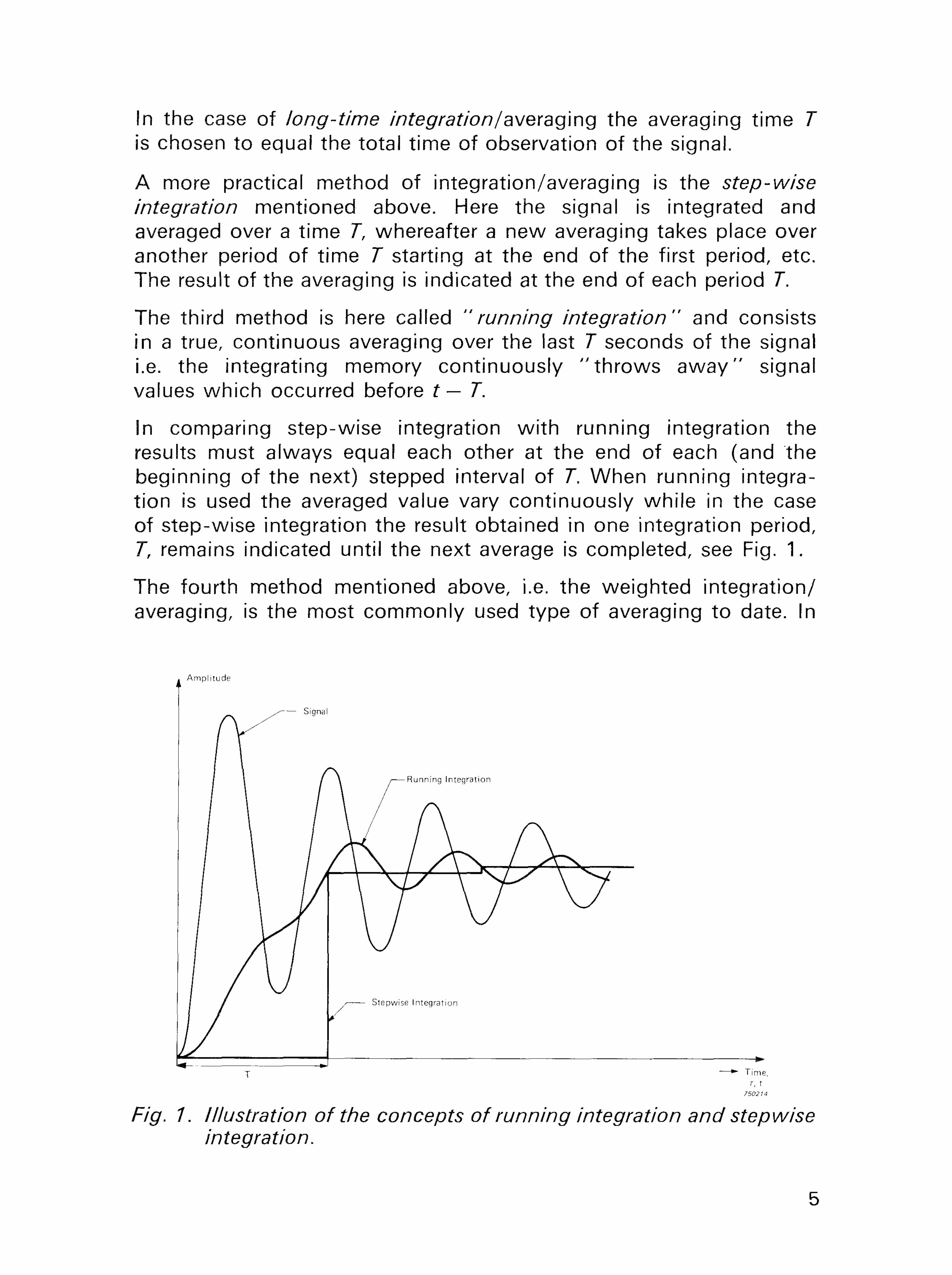
The third method is here called "running integration" and consists in a true, continuous averaging over the last T seconds of the signal i.e. the integrating memory continuously " th rows a w a y " signal values which occurred before t — T.

In comparing step-wise integration with running integration the results must always equal each other at the end of each (and the beginning of the next) stepped interval of 7". When running integra­tion is used the averaged value vary continuously while in the case of step-wise integration the result obtained in one integration period, T, remains indicated until the next average is completed, see Fig. 1.

The fourth method mentioned above, i.e. the weighted integration/ averaging, is the most commonly used type of averaging to date. In

Fig. 1. Illustration of the concepts of running integration and stepwise integration.

5

analog type measuring instruments the weighting is normally exponen­tial and is derived from R-C averaging circuits.

While the running integration/averaging weight each instantaneous value of the signal within T equally, the weighted averaging may give greater weight to signal values occurring at the instant of mea­surement than to signal values occurring, say T seconds earlier.

The main purpose of this article is, under different measurement conditions, to compare the different types of averaging techniques. Such a comparison should then enable the practicing engineer to better judge the limitations imposed upon the measurement by the averaging system, and to choose the parameters involved so as to obtain optimum results. This is of particular importance when the measured results are to be converted into digital form for further data processing.

2. T i m e and Frequency D o m a i n Desc r i p t i ons o f t h e A v e r a g i n g Process

As time and frequency are dual quantities, it is possible to study the time averaging process either in the time domain or in the frequency domain. Conversion from one domain to the other is, in this case, based on the so-called Fourier-transformation and the principle of superposition.

The Fourier transformation theorem states that :

F(u) = f(t)exp(-jut) dt

and

f(t)= ! F(u)exp(jut) df J — oo

where co = 2n/ , whi le the principle of superposition states tha t : In linear systems the effect of simultaneously superimposed actions is equal to the sum of the effects of each individual action.

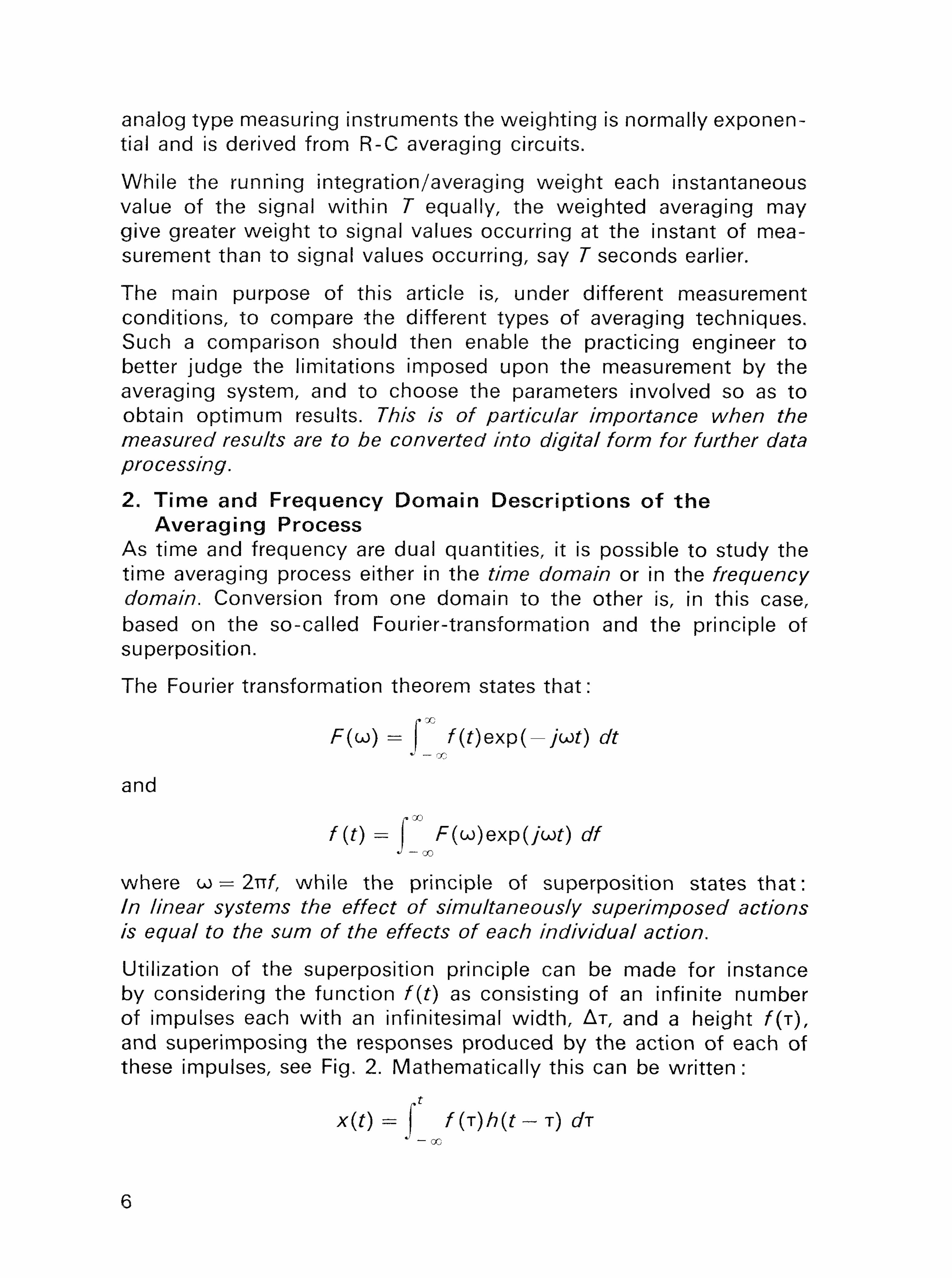
Utilization of the superposition principle can be made for instance by considering the function f(t) as consisting of an infinite number of impulses each with an infinitesimal width, AT , and a height f(r), and superimposing the responses produced by the action of each of these impulses, see Fig. 2. Mathematically this can be wr i t ten:

x(t) = f(T)h(t-T) dr J - o c

6

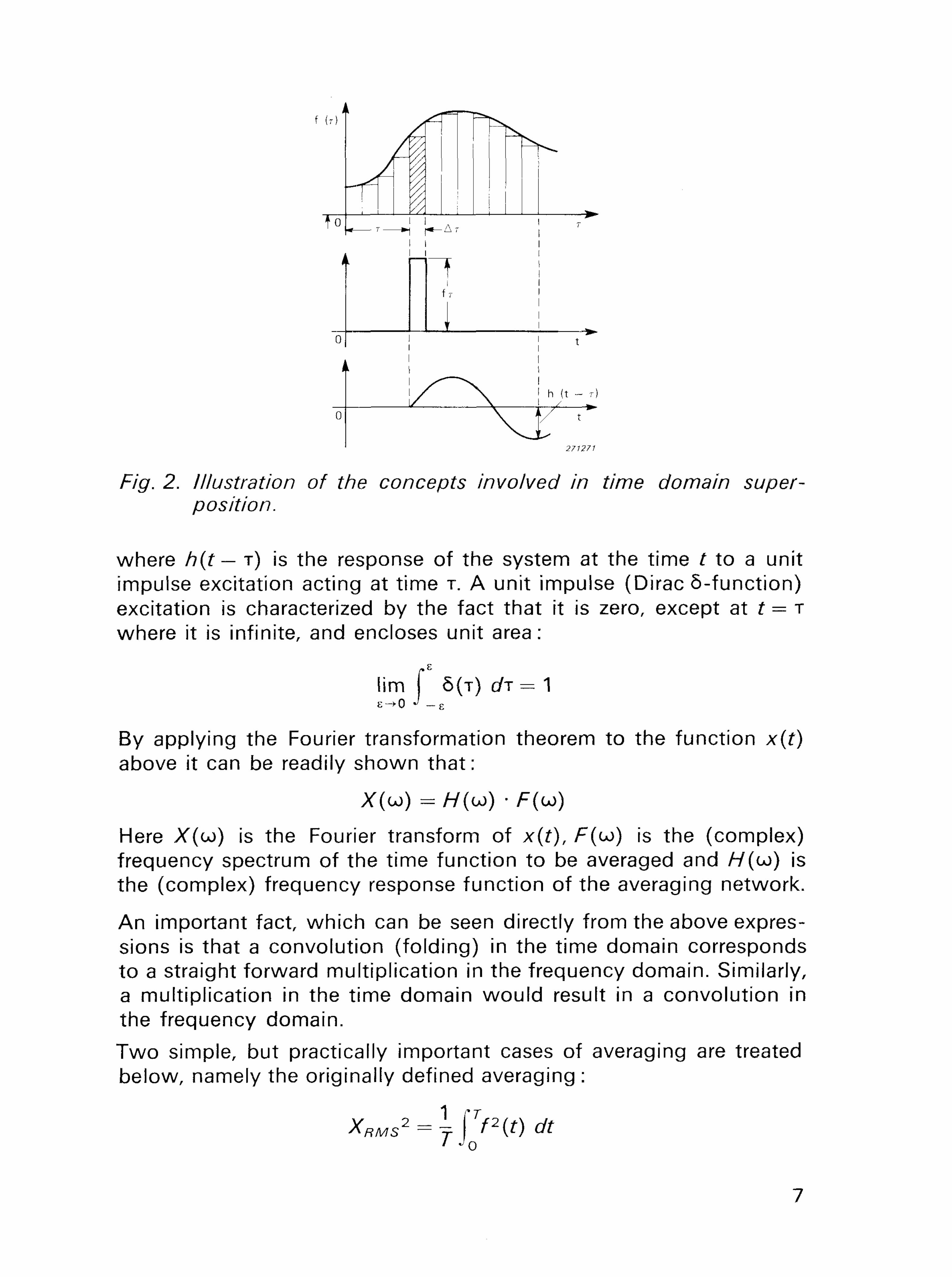
Fig. 2. Illustration of the concepts involved in time domain super­position.

where h(t — T) is the response of the system at the time M o a unit impulse excitation acting at time T. A unit impulse (Dirac 5-function) excitation is characterized by the fact that it is zero, except at t = r where it is infinite, and encloses unit area:

lim 5 ( T ) dr = 1 £->0 J - e

By applying the Fourier transformation theorem to the function x(t) above it can be readily shown that :

X (w ) = / / ( C J ) -F(u>)

Here X(co) is the Fourier transform of x(t), F(^) is the (complex) frequency spectrum of the time function to be averaged and H(LO) is the (complex) frequency response function of the averaging network.

An important fact, which can be seen directly from the above expres­sions is that a convolution (folding) in the time domain corresponds to a straight forward multiplication in the frequency domain. Similarly, a multiplication in the time domain would result in a convolution in the frequency domain. Two simple, but practically important cases of averaging are treated below, namely the originally defined averaging :

/ J0

7

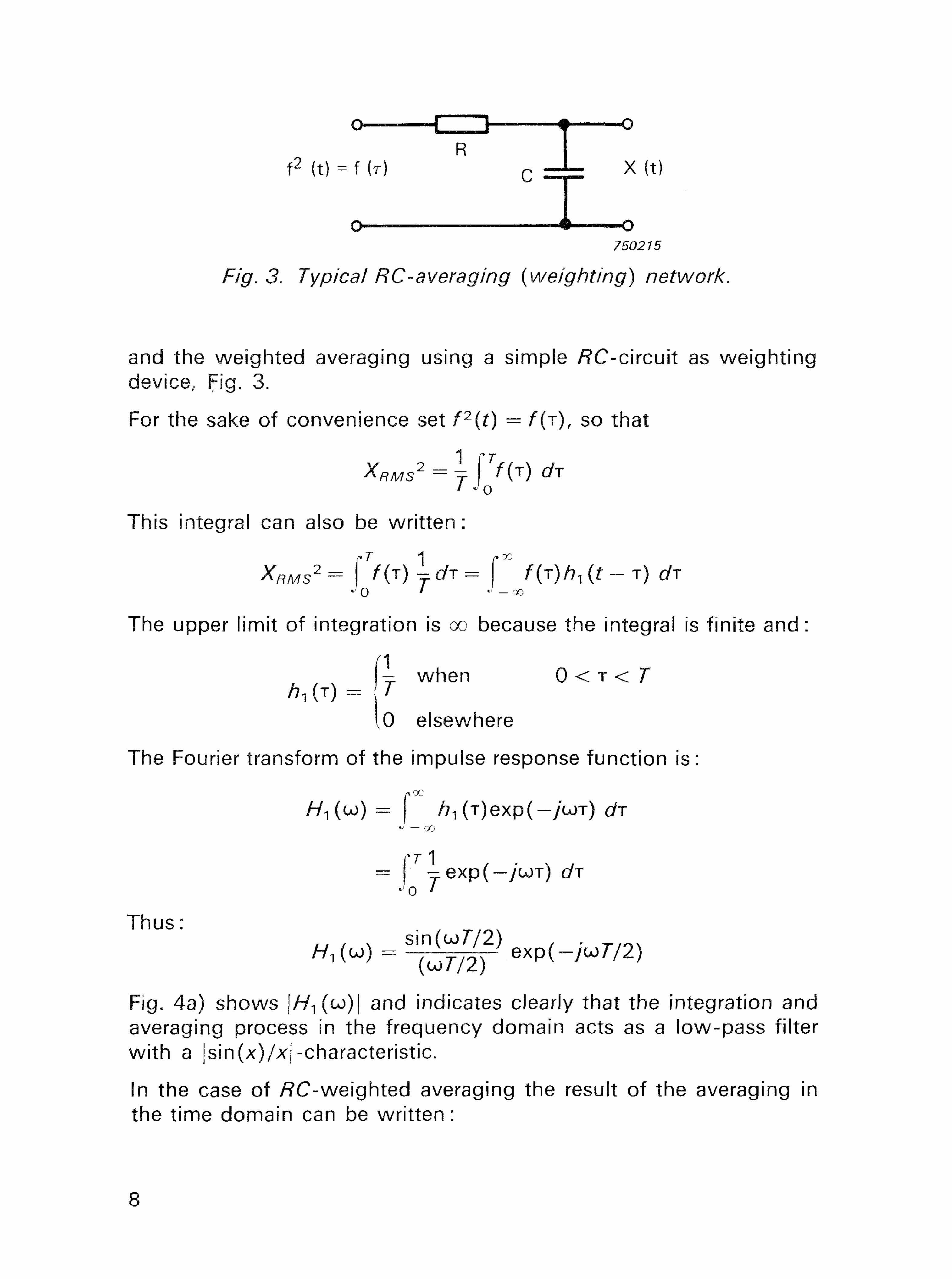
Fig. 3. Typical RC-averaging (weighting) network.

and the weighted averaging using a simple /?C-circuit as weighting device, Fig. 3.

For the sake of convenience set f2(t) = f(r), SO that

XRMS2 = l\Tf(T)dT

I J0

This integral can also be wri t ten: * * M S 2 = I f (T) y </T = / ( T ) / ^ (t - T) t/T

The upper limit of integration is GO because the integral is finite and:

- when 0 < x < 7

0 elsewhere

The Fourier transform of the impulse response function is:

H^(^) = /?1 (T)exp(—/OJT) tfr J — CO

= - e x p ( - y u ) T ) GTT

• 0 '

T h U S : ■ / T/OX . . sin(ojf/2) .

Fig. 4a) shows |/-/ i(w)| and indicates clearly that the integration and averaging process in the frequency domain acts as a low-pass filter with a |sin(x)/x|-characteristic.

In the case of /?C-weighted averaging the result of the averaging in the time domain can be written :

8

Fig. 4. Response characteristics in the frequency domain for a) True integration/averaging h) RC-weighted integration/averaging

XRMS2(t)= f f (T)h2(t ~ T) C/T J — 00

as the impulse response function for the /?C-weighting is: r

h2(r) = ~exp(-T/RC) T > 0

Here the Fourier transform of the impulse response function is:

H2(u) = KT^ e x p ( - T//?C)exp(-/'wT) ah-

The function |/y2(0J)i is plotted in Fig. 4b) and shows the well known frequency response of an /?-C-network.

3- Averaging of Random Signals When statistically fluctuating signals such as narrow band random

9

noise are measured the output signal from the detector wil l also fluctuate. These output signal fluctuations are then reduced by means of the averaging process.

One method of comparing different types of averaging processes is, consequently, to choose the averaging parameters in such a manner that the relative energy fluctuations in the averaged signal are the same, independently of the type of averaging system used. This method has been utilized by the authors in some earlier work, see Ref. (1), and is therefore only briefly outlined below.

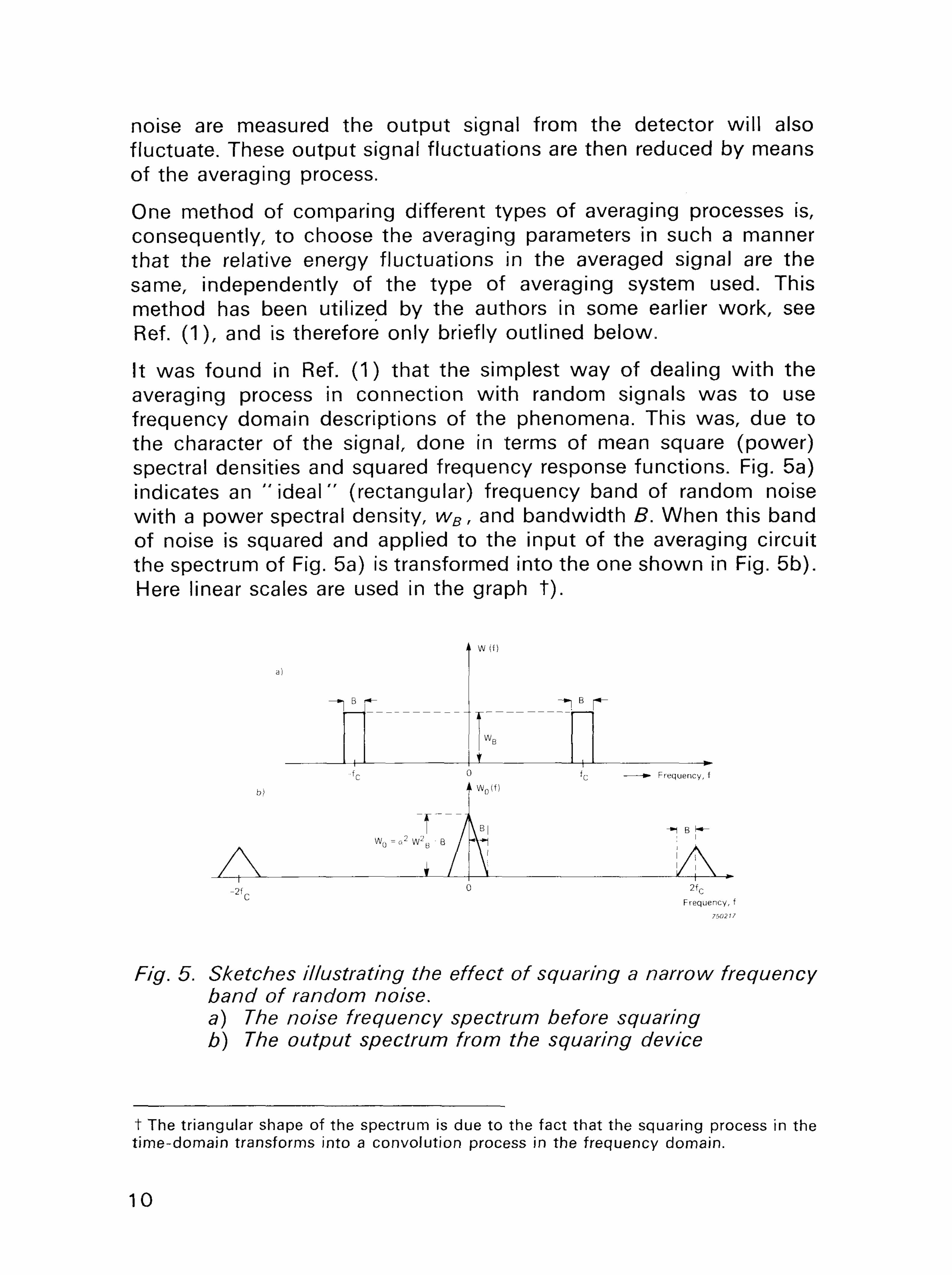
It was found in Ref. (1) that the simplest way of dealing with the averaging process in connection with random signals was to use frequency domain descriptions of the phenomena. This was, due to the character of the signal, done in terms of mean square (power) spectral densities and squared frequency response functions. Fig. 5a) indicates an " i d e a l " (rectangular) frequency band of random noise with a power spectral density, wBr and bandwidth B. When this band of noise is squared and applied to the input of the averaging circuit the spectrum of Fig. 5a) is transformed into the one shown in Fig. 5b). Here linear scales are used in the graph t ) .

Fig. 5. Sketches illustrating the effect of squaring a narrow frequency band of random noise. a) The noise frequency spectrum before squaring b) The output spectrum from the squaring device

t The triangular shape of the spectrum is due to the fact that the squaring process in the t ime-domain transforms into a convolut ion process in the frequency domain.

10

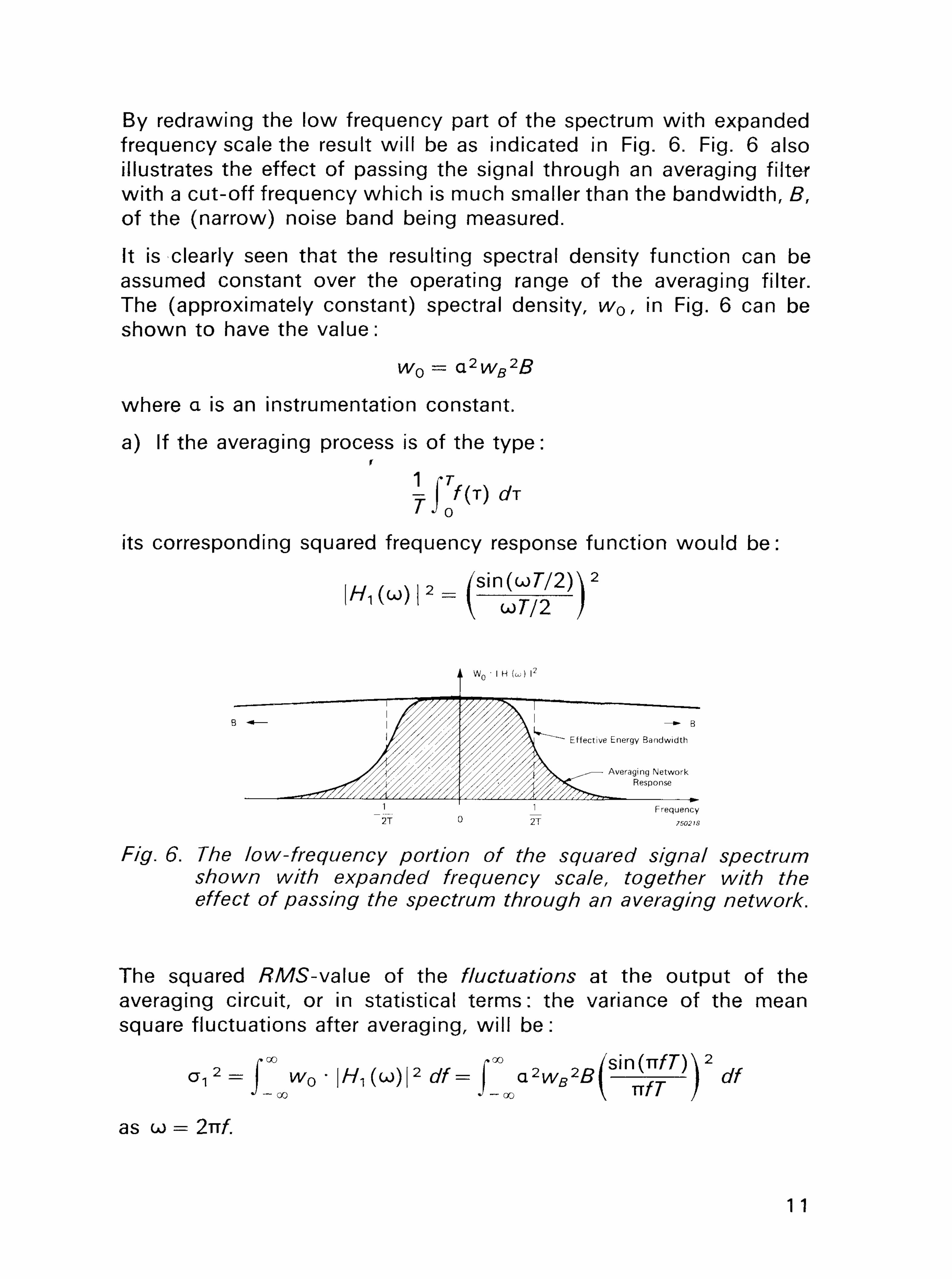
By redrawing the low frequency part of the spectrum with expanded frequency scale the result wil l be as indicated in Fig. 6. Fig. 6 also illustrates the effect of passing the signal through an averaging filter with a cut-off frequency which is much smaller than the bandwidth, B, of the (narrow) noise band being measured.

It is clearly seen that the resulting spectral density function can be assumed constant over the operating range of the averaging filter. The (approximately constant) spectral density, w0, in Fig. 6 can be shown to have the value:

w0 = a2wB2B

where a is an instrumentation constant.

a) If the averaging process is of the type:

its corresponding squared frequency response function would be:

i"i<«>i"pi$F)a

Fig. 6. The low-frequency portion of the squared signal spectrum shown with expanded frequency scale, together with the effect of passing the spectrum through an averaging network.

The squared /?MS-value of the fluctuations at the output of the averaging circuit, or in statistical terms: the variance of the mean square fluctuations after averaging, wil l be:

O, 2 = f w 0 ' \H, (U))|2 df= J ^ Q 2 W s 2 f l ^ 5 ! ! 1 ^ 3 ^ 2 df

as u> = 2TTA

11

Thus

R Q l

2 = a2wB2j

or:

a, = *wB J^ Now, the mean square value of an " i d e a l " band of random noise with constant spectral density is:

E' =wBB

and, taking the instrumentation constant, a, into account:

E = awB B

The relative energy fluctuations at the output of the averager is thus:

a-! _ awfl VB/t E awB B

or:

a., 1

b) If the averaging process is of the /?C-weighted type then the squared frequency response function would be:

1 1

W h e r e / ° = 2 ^ C "

Substituting this kind of averaging for the one treated above results in a variance of the mean square fluctuations after averaging of:

r00 df o2

2 = a2wB2B = a2wB

2Bnf0 J-oo I + \tl*0)

and :

a 2 = awByfBTyf0

whereby the relative energy fluctuations at the output of the averager becomes:

12

a 2 __ awBVBr\'f0

E awBB

or:

E V £ ^/2B~RC ■ ^ - ^ ^ ■■ ■ M L — _ ■ _ _

Equating the relative energy fluctuations at the output of the two kinds of averagers one obtains:

1 / r r / 0 _ 1 JBT N B J2BRC

or: I

T= ~ = 2RC TXf0

I . I

where f0 is the 3 dB upper limiting frequency of the /?C-network (Fig. 4b). Another fact which is worth noting in connection with the above derivations is that because the comparison has been based on energy considerations also the energy (or noise) bandwidths of the two averagers are the same.

4. Averaging of Periodic Signals Two important types of periodic signals are considered in the fol lowing because they represent " limiting " cases. The first type of signal is the simple (harmonic) sine-wave, while the second type consists of an " i n f i n i t e " train of periodically repeated S-functions.

In the case of the simple sine wave signal'the use of frequency domain descriptions may again prove to be the most straight forward method of dealing with the problem.

Considering the signal to be measured to be given by:

x(t) = X0 sin (oof)

where CJ = 2rrf, the "ene rgy " signal at the input to the averager would be:

f(T) = ax2(t) = aX02 sin2(oox) = ^ ~ (1 - COS(2CJT))

where, once again, a is an instrumentation constant. Fig. 7 shows this signal both in the time domain and in the frequency domain, and it is readily seen that it consists of a DC-component, (a /2 )X 0

2 ,

13

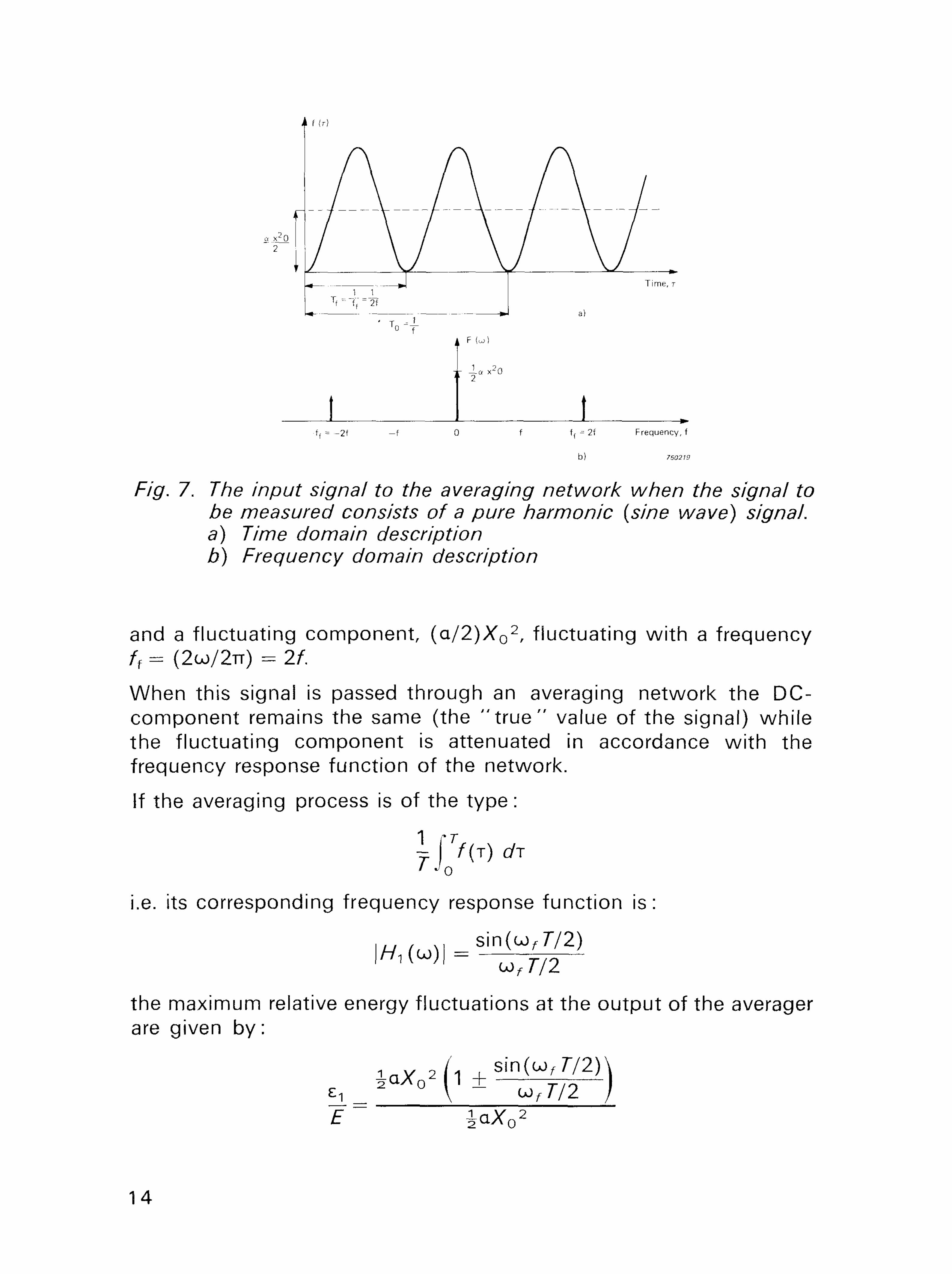
Fig. 7. The input signal to the averaging network when the signal to be measured consists of a pure harmonic (sine wave) signal. a) Time domain description b) Frequency domain description

and a fluctuating component, ( a /2 )X 02 , f luctuating wi th a frequency

ff - (2CO/2TT) - 2f.

When this signal is passed through an averaging network the DC-component remains the same (the " t r u e " value of the signal) whi le the fluctuating component is attenuated in accordance with the frequency response function of the network.

If the averaging process is of the type:

7.I?(T) dT

i.e. its corresponding frequency response function is:

sin(u,772)

the maximum relative energy fluctuations at the output of the averager are given by :

£i ^ (i ± ^p)

14

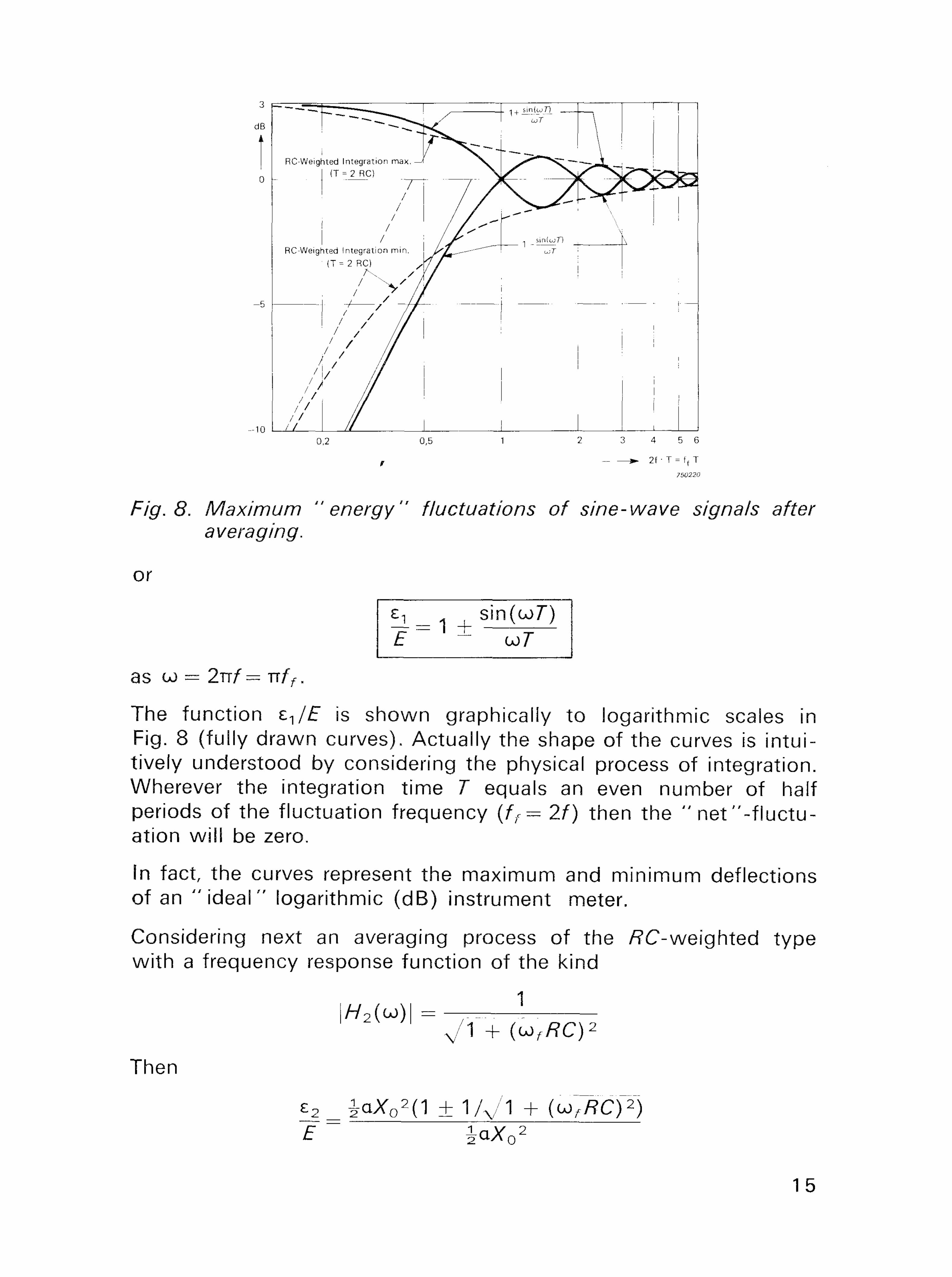
Fig. 8. Maximum "energy" fluctuations of sine-wave signals after averaging.

or

Zj_ s'm(uT) E " ' - oor

as u) = 2TT/= rr/f,

The function £-,/£ is shown graphically to logarithmic scales in Fig. 8 (fully drawn curves). Actually the shape of the curves is intui­tively understood by considering the physical process of integration. Wherever the integration time T equals an even number of half periods of the fluctuation frequency (ff= 2f) then the " net " - f luc tu­ation wil l be zero.

in fact, the curves represent the maximum and minimum deflections of an " i d e a l " logarithmic (dB) instrument meter.

Considering next an averaging process of the /?C-weighted type with a frequency response function of the kind

\H2{u)\= ..... \ V / 1 +(U), /?C)2

Then

£2 = ^aX 02(1 + 1 / V 1 + (u^C)" 2 " ) E iaX 0

2

15

or:

- | = 1 +— ._. E V / 1 + (2co/?C)2

as again GO = 2uf = TT/> = co f/2.

Setting T = 2/?C gives: £ 2 " " 1

^ ~ ±Vl+(^7=)"2

The function £ 2 /£ is also plotted in Fig. 8 (dotted curves) and shows that when T is chosen to equal 2 RC, as postulated for narrow band random noise, then, in the case of harmonic signals, the maximum fluctuations at the output of the averager are the same for the two kinds of averagerst.

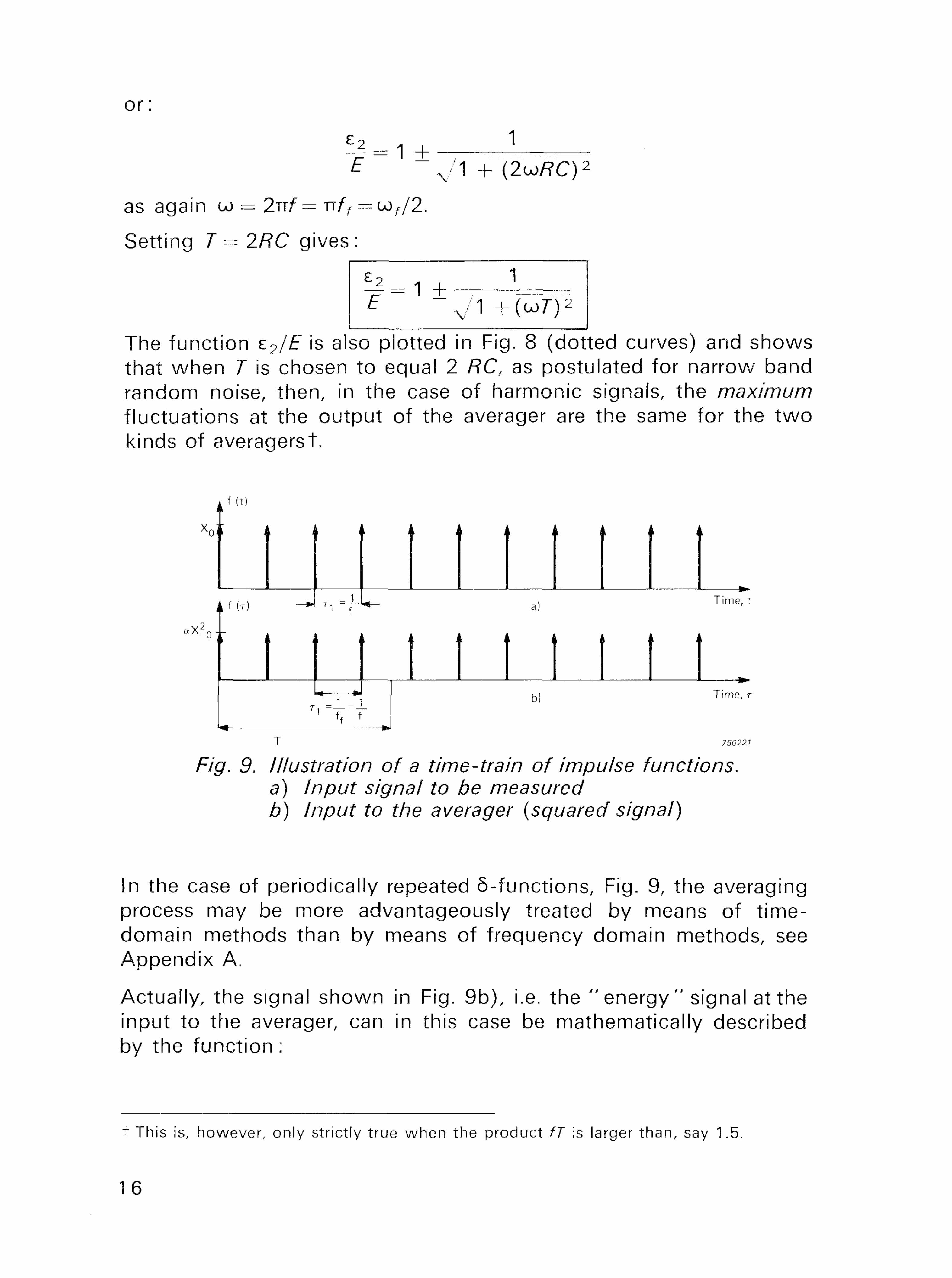
Fig. 9. Illustration of a time-train of impulse functions. a) Input signal to he measured b) Input to the averager {squared signal)

In the case of periodically repeated S-functions, Fig. 9, the averaging process may be more advantageously treated by means of t ime-domain methods than by means of frequency domain methods, see Appendix A.

Actually, the signal shown in Fig. 9b), i.e. the " energy " signal at the input to the averager, can in this case be mathematically described by the function :

f This is, however, only strictly true when the product fj is larger than, say 1.5.

16

f(T) = a X 02 I 5 ( T - A 7 T l )

n

where T V is the repetition period, and 5 ( T — nr^) describes 5-functions (unit impulse functions) occurring at times T = nr^.

If the averager is the type

j \ f(T) Cfj

the relative " energy "-f luctuations, r\JEf can be expressed as:

where f= 1 / T V and T = nr^ + TX (Fig. 9b)) . /? = 0, 1, 2, 3, etc.

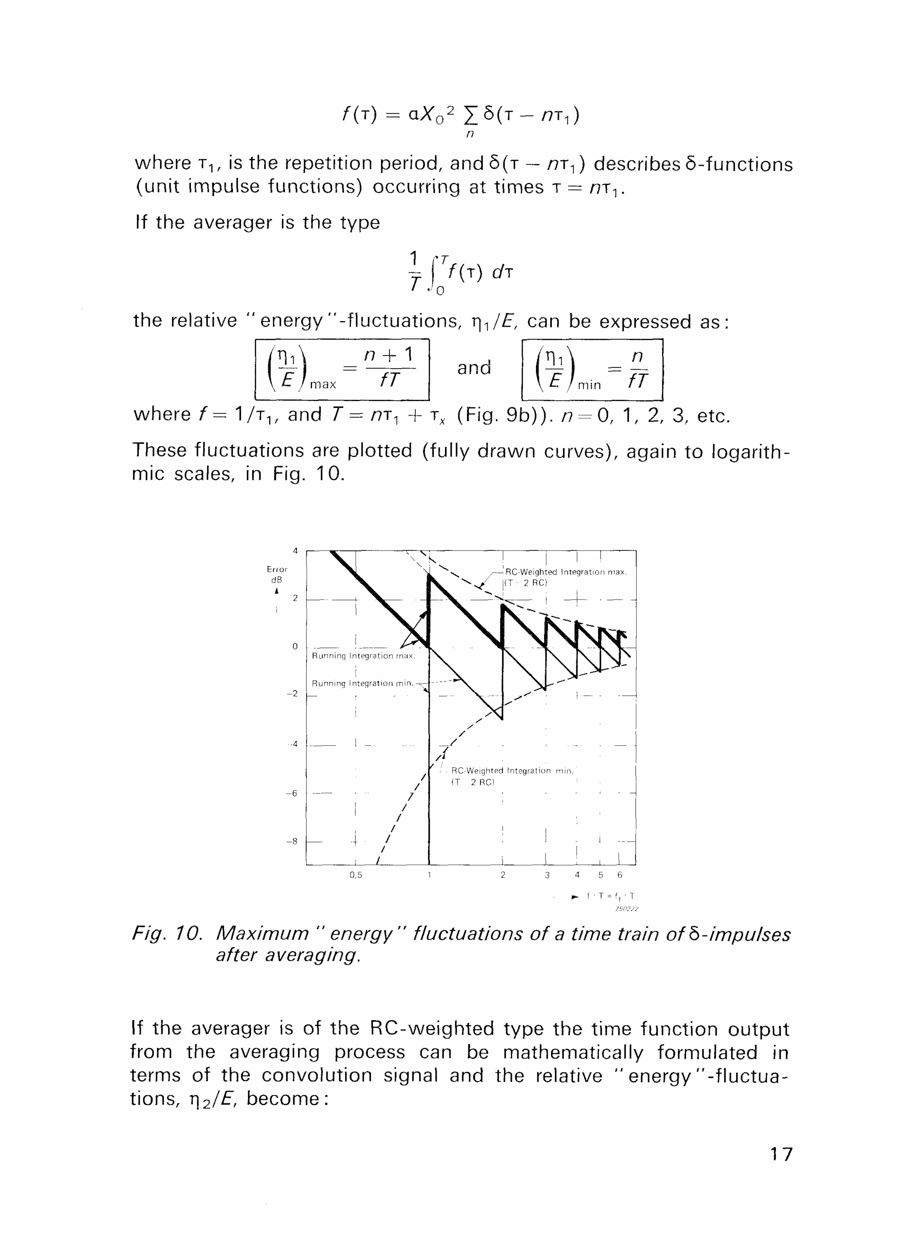
These fluctuations are plotted (fully drawn curves), again to logarith­mic scales, in Fig. 10.

Fig. 70. Max/mum " energy" fluctuations of a time train ofb-impulses after averaging.

If the averager is of the RC-weighted type the time function output from the averaging process can be mathematically formulated in terms of the convolution signal and the relative " energy "- f luctua­tions, n 2 /£ , become:

17

m = ? \ £ / m a x fTQ - e x p ( - 2 / / 7 - ) )

and

\ £ / m i n fT(exp{2/fT) --\)

Also these functions are plotted in Fig. 10 (dotted curves), and again / = 1/-T, and 7"= 2 /?C.

Note that even in this case the relative fluctuations in the /?C-weighted averaging practically envelopes the fluctuations in the running inte­gration type of averaging.

References

1. BROCH, J . T. and W A H R M A N , C. G.: Effective Averaging Time of Level Recorders. Bruel & Kjaer Technical Review No. 1-1961.

2. W A H R M A N , C. G.: ATrue RMS Instrument. Bruel & Kjaer Technical Review No. 3-1958.

3. W A H R M A N , C. G.: Methods of Checking the RMS Properties of RMS Instruments. Bruel & Kjaer Technical Review No. 1-1963.

4. W A H R M A N , C. G.: Impulse Noise Measurements. Bruel & Kjaer Technical Review No. 1-1969.

5. RICE, S. 0 . : Mathematical Analysis of Random Noise. Bell System. Techn. Journal 23 (1944) and 24 (1945). Also contained in N. Wax.: " Selected Papers on Noise and Stochastic Processes". Dover Publications, Inc. New York 1954.

APPENDIX A

Averaging of Periodically Repeated b-Functions As stated in the main text of this paper the averaging of periodically repeated 6-function is best studied in terms of t ime-domain methods.

Considering first the case of running integration the output from the averager would have the fo rm:

aX02 "T v ~, x ,

T]i = - y ^ I & ( T - m,) dr 1 J 0 n

or

O.XQ2 V c / \ / T]1 = - ^ -1 5 ( T - ^ ) dJ

1 n J0

18

The evaluation of this expression depends upon the relationship between T, T and A?TV and may be best understood by the fol lowing reasoning :

The summation of the 5-function integral, i.e.:

X 5 ( T — PT^) dr n - 0

actually expresses how many unit impulses are within the integration interval T. I t for instance, 0 ^ T <̂ T V only one impulse (or none) is inside the integration interval. The output from the averager wi l l therefore fluctuate between 0 and a maximum value of a - (X0

2/T). It is readily seen that this maximum value decreases hyperbolically as T increases.

When T becomes larger than T V then either one or two impulses are included in the averaging process. In general, therefore, when T is larger than T., the maximum value of the fluctuations can be mathe­matically described in the fo rm:

(Ti1)max = ^ -=^- I \T&(T- PTi) C/T

_ a X 02 ( / 7 + 1 ) .

m, + TX

where/7T1 + TX = T and 0 ^ TX <L T.,

Similarly the minimum value of the fluctuations is given by :

( n ) . _ aXo2n

The " t r u e " average of the signal is:

and introducing / = 1 / T 1 / the relative " e n e r g y " fluctuations, T ^ / E become:

\E)ma, = rLfr a n d \Ejmm = ^

In the case of /?C-weighted averaging the output from the averager is again obtained by means of time domain convolution and takes the form :

19

or

n2 = -Sp- I I 6(T-A7Tl)exp[-(f-T)//?C] dr nc n J0

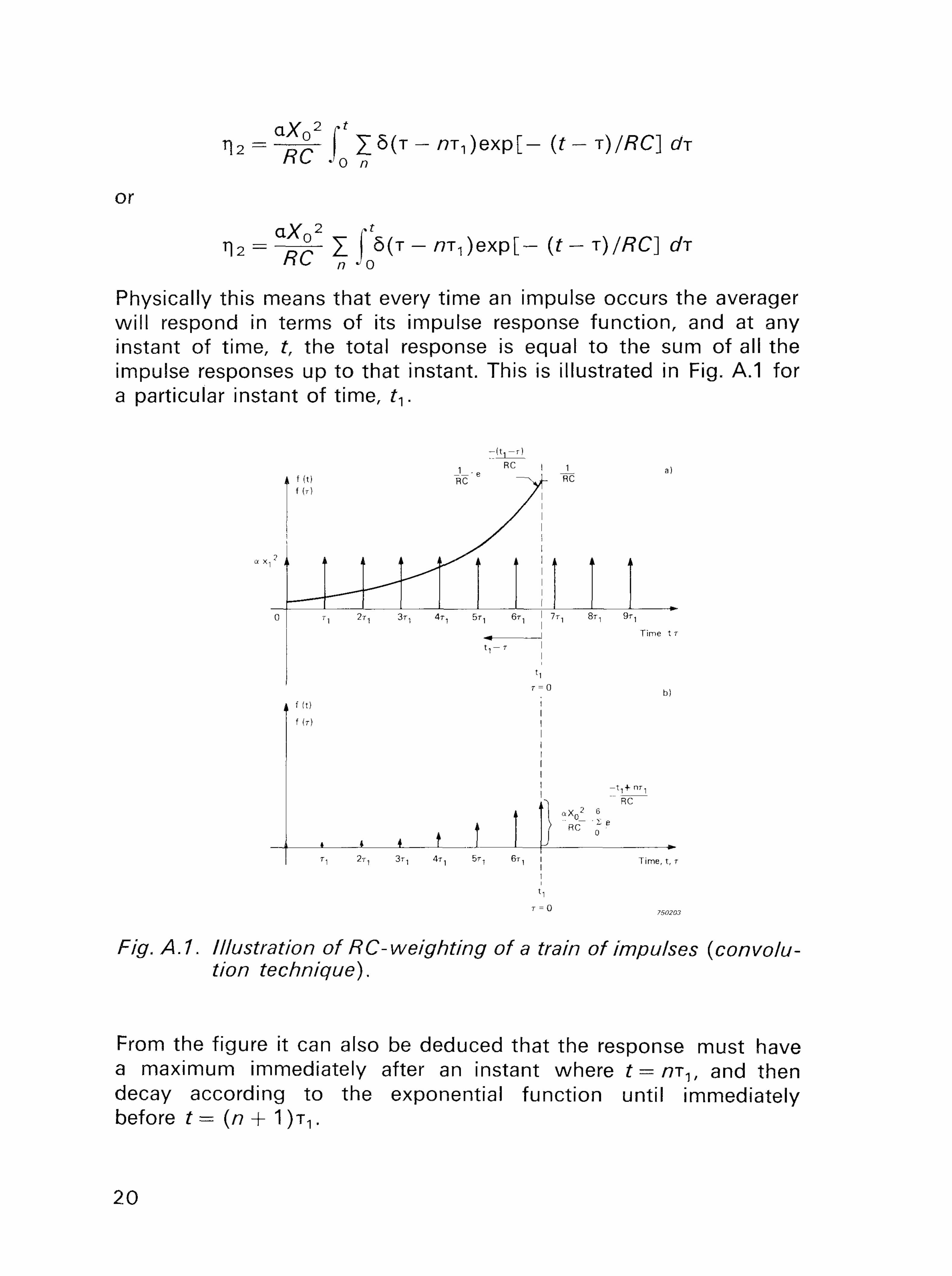
Physically this means that every time an impulse occurs the averager wil l respond in terms of its impulse response function, and at any instant of time, t, the total response is equal to the sum of all the impulse responses up to that instant. This is illustrated in Fig. A.1 for a particular instant of time, f v

Fig. A.I. Illustration of RC-weighting of a train of impulses {convolu­tion technique).

From the figure it can also be deduced that the response must have a maximum immediately after an instant where t=m^, and then decay according to the exponential function until immediately before t= (n + 1 ) T V

20

The maximum value is obviously

aX 2 n

(n2)max = -£~- I e x p ( - mJRC)

and the minimum value:

aX 2 n

(n2)min = - 5 ^ - I e x p ( - (/?+ 1)T1//?C)= (r)2)max eXP ( - Tl//?C)

The absolute maximum is (theoretically) reached when n -> oo and the sum then represents an infinite geometric progression:

CO

K e x p f - V f l C ) ) "

and as exp(— T^/RC) < 1 then:

„ l , ( a X p ( - T l / / ? C »" = 1 -exp( 1 - T < / / ? C ) Again the " t r u e " average of the signal is:

£ = o Y o f Ti

whereby

/Tb\ (Ti//?C) U/max 1 -expC-T./ZTC)

The minimum value of the relative fluctuations can now be obtained from:

Introducing 7"= 2/?C and / = 1 / T V the results can be written :

m = ? \f/max /7(1 -exp(-2//7))

and

\£ /m in fT(exp(2/fT) - 1)

21

Averaging Time of Level Recorder Type 2306 and "Fast" and "S low" Response of Level Recorders 2 3 0 5 / 0 6 / 0 7

by

K. Zaveri, M. Phil.

ABSTRACT The averaging time of Level Recorder Type 2 3 0 6 was determined for its various wri t ing speeds. Investigations were also carried out to determine the most suitable wr i t ing speeds that would simulate pen fluctuations of a Level Recorder w i th the meter needle deflections of a Sound Level Meter. For small pen f luctuations wri t ing speeds of Level Recorders Types 2 3 0 5 / 0 6 / 0 7 are suggested for AC and DC recording that w i l l yield the best correlation.

S O M M A I R E Le temps d'integration de I'Enregistreur de Niveau Type 2 3 0 6 a ete determine pour les dif-ferentes vitesses d'ecriture de I'appareil. On a egalement cherche a determiner les vitesses d'ecriture qui permettent d'obtenir des f luctuations du systeme d'ecriture simulant les deflex­ions de I'aiguille d'un sonometre. Pour de petites f luctuations, on suggere les vitesses d'ecri­ture des Enregistreurs de Niveau Types 2 3 0 5 / 0 6 / 0 7 donnant, pour les enregistrements en alternatif et en cont inu, la meilleure correlation.

Z U S A M M E N F A S S U N G Die Mittlungszeit des Pegelschreibers Typ 2 3 0 6 wurde in Abhangigkeit von der einstellba-ren Schreibgeschwindtgkeit bestimmt. Auch wurden Untersuchungen angestellt, urn diejeni-gen Schreibgeschwindigkeiten herauszufinden, bei denen die Schreibstiftschwankungen ei-nes Pegelschreibers mit den Zeigerausschiagen eines Schallpegelmessers bestmoglich korre-spondieren. Fur Gleich- und Wechselspannungsaufzeichnung mit den Pegelschreibern 2 3 0 5 / 0 6 / 0 7 werden Einstellungen vorgeschlagen, fur die bei kleinen Ausschiagen die be-ste Ubereinstimmung erzielt w i rd .

Introduction Since the publication of Technical Review No. 1 1974 , describing the measurement of Averaging Times of Level Recorders Types 2 3 0 5 and 2 3 0 7 , Bruel & Kjaer have developed a transportable Level Recorder Type 2 3 0 6 . The Averaging Time of this Level Recorder is determined and the results presented as a function of its wr i t ing speed in Part I of this article.

22

Furthermore, the desire to try to correlate the meter response of con­ventional Sound Level Meters w i th level recorder pen f luctuat ions, has lead to the investigations described in Part II of this article. However, the task of simulation of meter needle deflections w i th pen f luctuations on the Level Recorder paper is not as simple and direct as one might ex­pect at first sight. The main reason for this is that the modes of opera­tion and thus the dynamics of the Sound Level Meter and the Level Re­corder are basically different. Whi le the definit ion of "Fast" and " S l o w " response, primarily intended for Sound Level Meter, is based on tone burst response, such a def ini t ion, as wi l l be shown by the results, is not suitable for a Level Recorder as its response is dependent on the amplitude levels of tone bursts.

The fol lowing three types of experiments were carried out:

a) Direct comparison of Meter Needle deflections of a Sound Level Me­ter w i th pen f luctuations of a Level Recorder at different wr i t ing speeds for a narrow band random noise input.

b) Measuring the frequency response characteristic of the Sound Level Meter and the Level Recorder for a 10 kHz carrier frequency signal input, amplitude modulated by a low frequency sinusoid.

c) Determining Level Recorder response to tone burst signals (cfr. IEC 179).

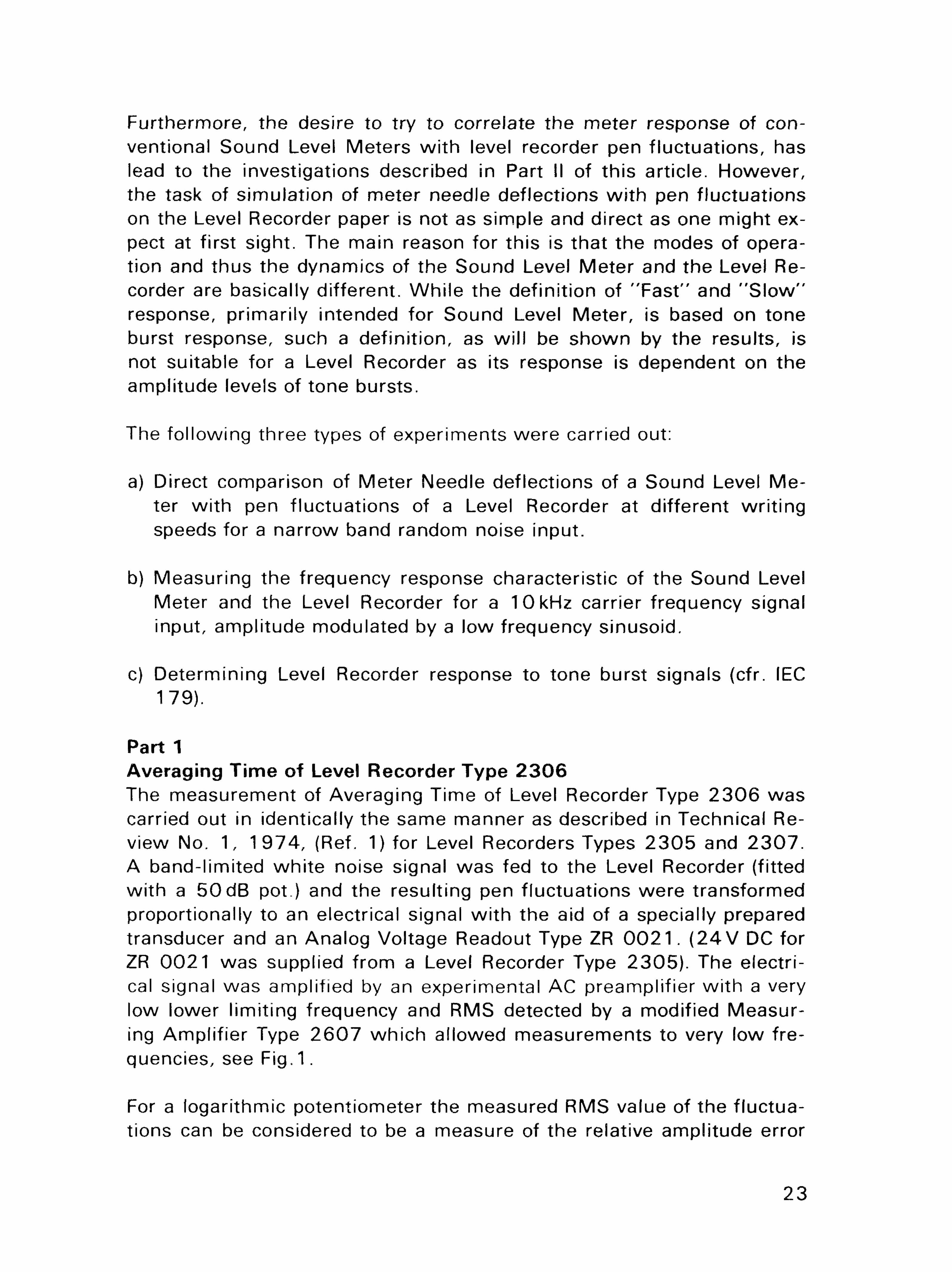
Part 1 Averaging Time of Level Recorder Type 2 3 0 6 The measurement of Averaging Time of Level Recorder Type 2 3 0 6 was carried out in identically the same manner as described in Technical Re­view No. 1 , 1 9 7 4 , (Ref. 1) for Level Recorders Types 2 3 0 5 and 2 3 0 7 . A band-limited whi te noise signal was fed to the Level Recorder (fitted w i th a 5 0 d B pot.) and the resulting pen f luctuations were transformed proportionally to an electrical signal w i th the aid of a specially prepared transducer and an Analog Voltage Readout Type ZR 0 0 2 1 . ( 2 4 V DC for ZR 0 0 2 1 was supplied from a Level Recorder Type 2305) . The electri­cal signal was amplified by an experimental AC preamplifier w i th a very low lower l imiting frequency and RMS detected by a modified Measur­ing Amplif ier Type 2 6 0 7 which allowed measurements to very low fre­quencies, see Fig. 1.

For a logarithmic potentiometer the measured RMS value of the f luctua­tions can be considered to be a measure of the relative amplitude error

23

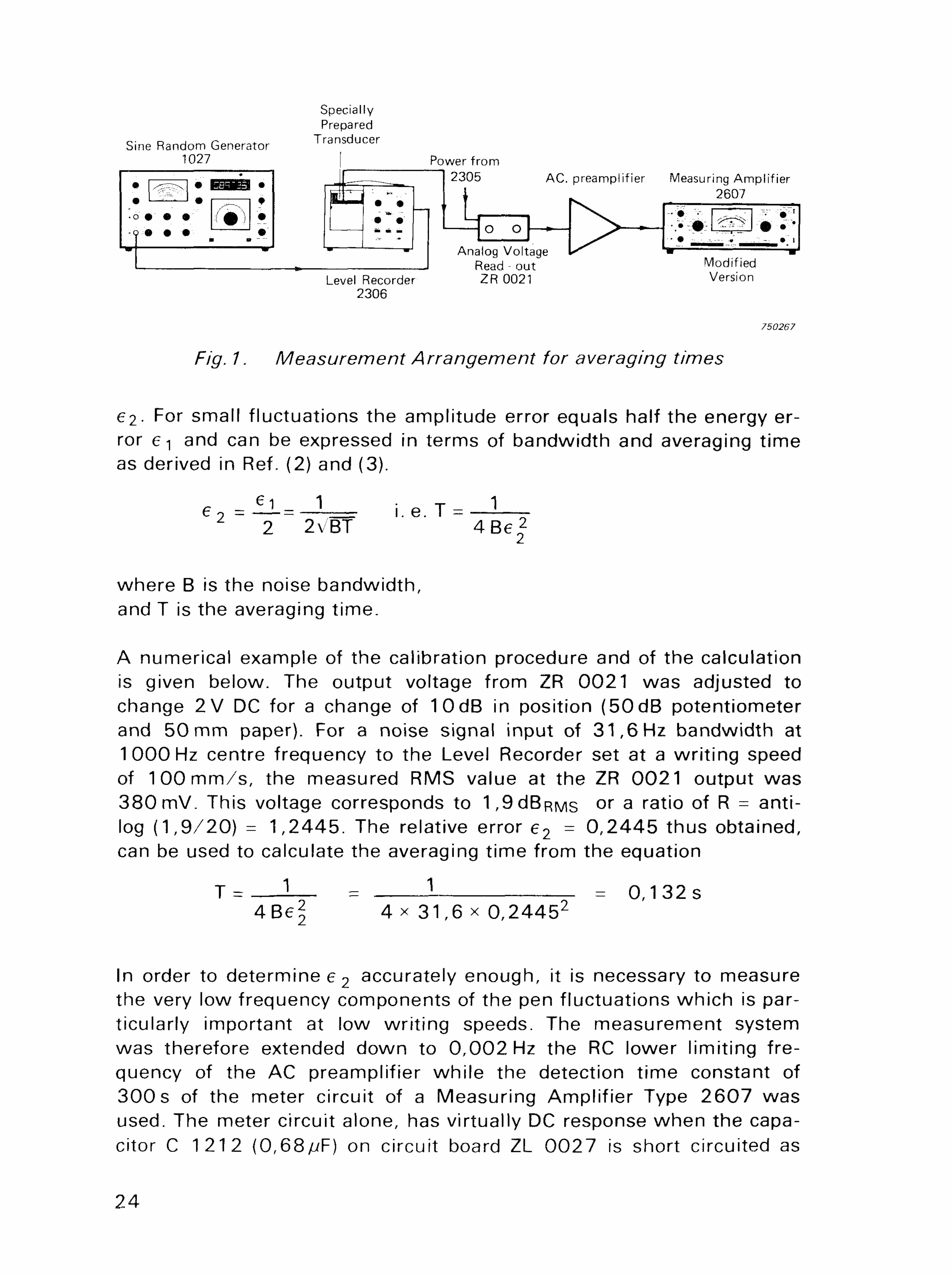
Fig. 7. Measurement Arrangement for averaging times

62- For small f luctuations the amplitude error equals half the energy er­ror e-| and can be expressed in terms of bandwidth and averaging t ime as derived in Ref. (2) and (3).

e 2 = i l = - l = i . e . T ^ - I — 1 2 2VBT 4 B e |

where B is the noise bandwidth, and T is the averaging t ime.

A numerical example of the calibration procedure and of the calculation is given below. The output voltage from ZR 0 0 2 1 was adjusted to change 2 V DC for a change of 10dB in position (50dB potentiometer and 50 mm paper). For a noise signal input of 31 ,6 Hz bandwidth at 1000 Hz centre frequency to the Level Recorder set at a wr i t ing speed of 1 0 0 m m / s , the measured RMS value at the ZR 0 0 2 1 output was 3 8 0 mV. This voltage corresponds to 1,9dBRMs o r a r a t i ° of R = anti-log ( 1 , 9 / 2 0 ) = 1,2445. The relative error e 2 = 0 ,2445 thus obtained, can be used to calculate the averaging t ime from the equation

T = ] — = J = 0 , 1 3 2 s 4 B e ^ 4 x 31 ,6 x 0 , 2 4 4 5 2

In order to determine e 2 accurately enough, it is necessary to measure the very low frequency components of the pen fluctuations which is par­ticularly important at low wr i t ing speeds. The measurement system was therefore extended down to 0 ,002 Hz the RC lower l imiting fre­quency of the AC preamplifier whi le the detection t ime constant of 3 0 0 s of the meter circuit of a Measuring Amplif ier Type 2 6 0 7 was used. The meter circuit alone, has virtually DC response when the capa­citor C 1212 (0,68yuF) on circuit board ZL 0 0 2 7 is short circuited as

24

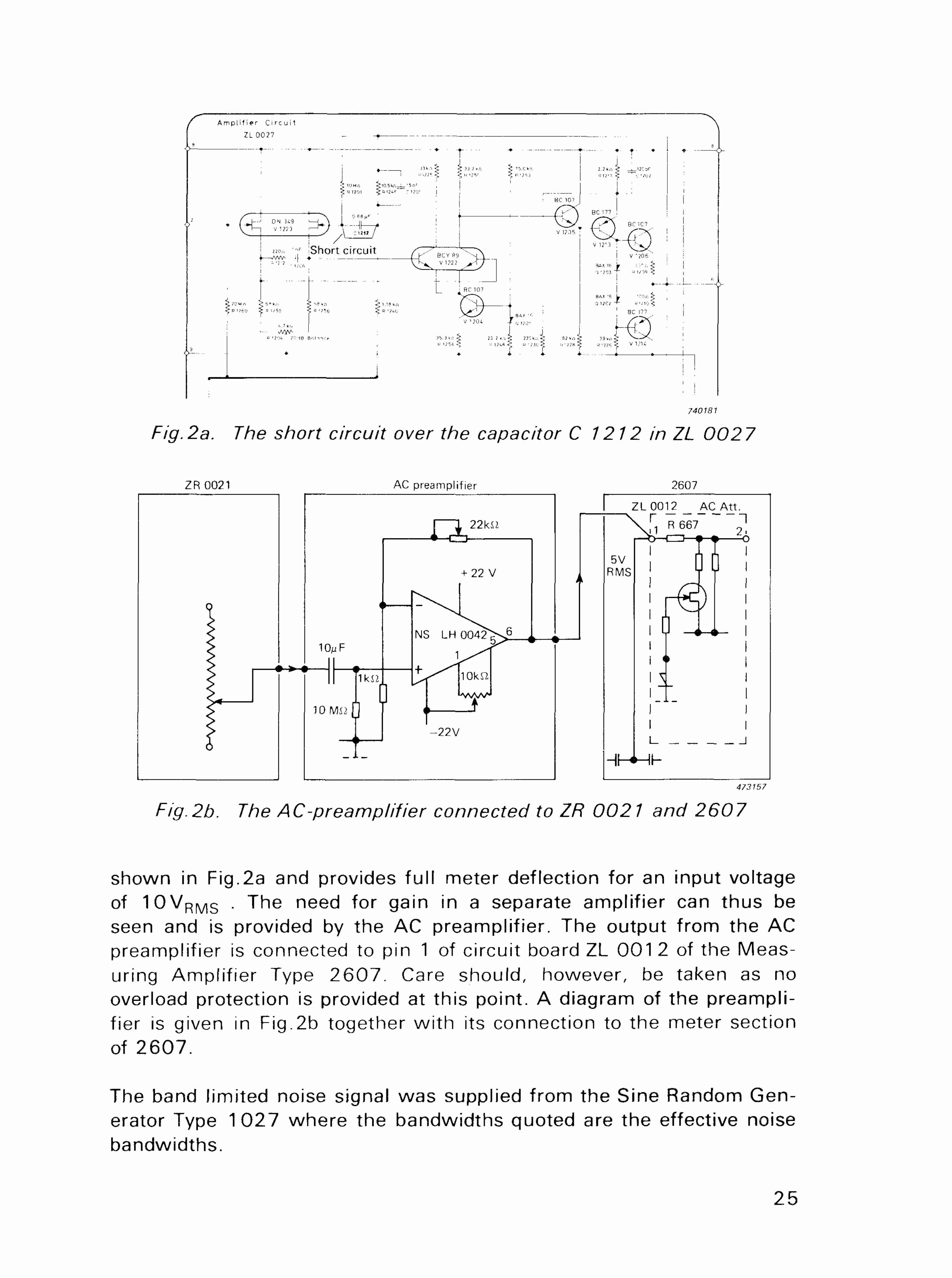
Fig.2a. The short circuit over the capacitor C 1212 in ZL 0027

Fig.2b. The AC-preamplifier connected to ZR 0027 and 2607

shown in Fig.2a and provides fu l l meter deflection for an input voltage of 1 0 V R M S . The need for gain in a separate amplif ier can thus be seen and is provided by the AC preamplif ier. The output f rom the AC preamplifier is connected to pin 1 of circuit board ZL 001 2 of the Meas­uring Ampl i f ier Type 2 6 0 7 . Care should, however, be taken as no overload protection is provided at this point. A diagram of the preampli­fier is given in Fig.2b together w i th its connection to the meter section of 2 6 0 7 .

The band l imited noise signal was supplied f rom the Sine Random Gen­erator Type 1 0 2 7 where the bandwidths quoted are the effective noise bandwidths.

25

T3

&

to

CO

I

CD

26

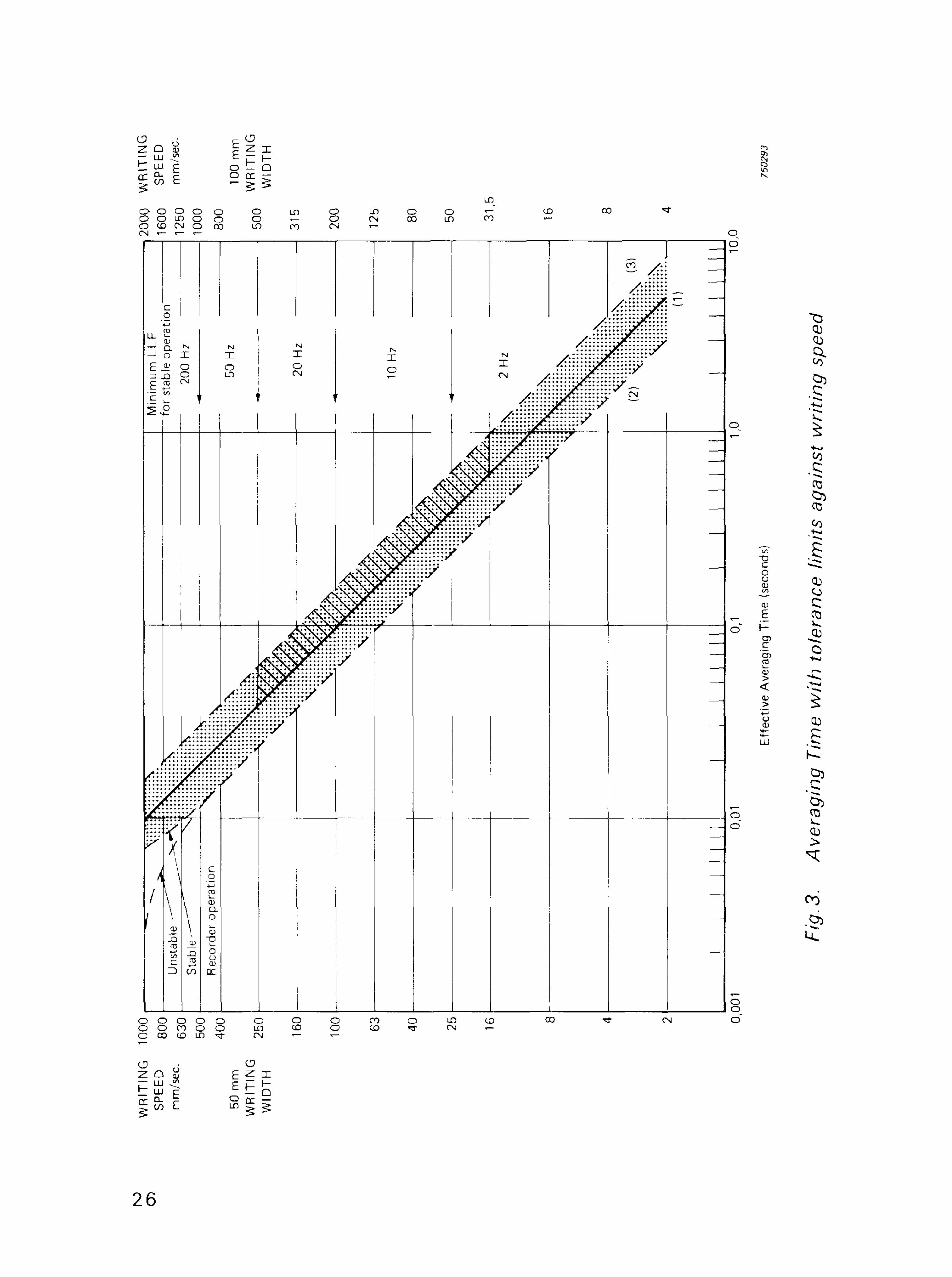
Measurement Results Experiments were carried out by applying different noise bandwidths to the Level Recorder and measuring the resultant various levels of pen f luctuat ions. Fig.3 shows a plot of averaging t ime against wr i t ing speed where the spread of results obtained for the Level Recorder Type 2 3 0 6 is shown by the double shaded area lying between curves 1 and 3 for the four wr i t ing speeds of 16, 4 0 , 1 0 0 and 2 5 0 m m / s . Curves 1 , 2 and 3, reproduced from Ref. (1), refer to the averaging t imes for Level Recorders Types 2 3 0 5 and 2 3 0 7 . Curve 2 also given in Ref. (2), gives the l imit ing curve for zero pen f luctuat ions; curve 1 represents the aver­aging t ime of Level Recorders 2 3 0 5 and 2 3 0 7 for normal Recorder Set­tings (described in Ref. 1), wh i le curve 3 is considered as the l imit ing curve for maximum al lowed pen f luctuat ions. As can be seen, the aver­aging t ime of Level Recorder Type 2 3 0 6 agrees reasonably wel l w i th those of Level Recorders 2 3 0 5 and 2 3 0 7 and curve 1 is suggested to be the nominal curve also for Level Recorder Type 2 3 0 6 .

Part 2 Simulation of "Fast" and " S l o w " Meter Time Constants on Level Recorders Fluctuating sound pressure levels when measured w i th sound level me­ters are averaged on the Meter according to Internationally accepted Time Constants "Fast " or " S l o w " . However, the frequent desire to ob­tain permanent records on Level Recorder paper of the sound pressure level requires determinat ion of the most suitable wr i t ing speed that s i ­mulates meter needle deflections as closely as possible. In the fol low­ing, three methods are described for determining appropriate wr i t ing speeds.

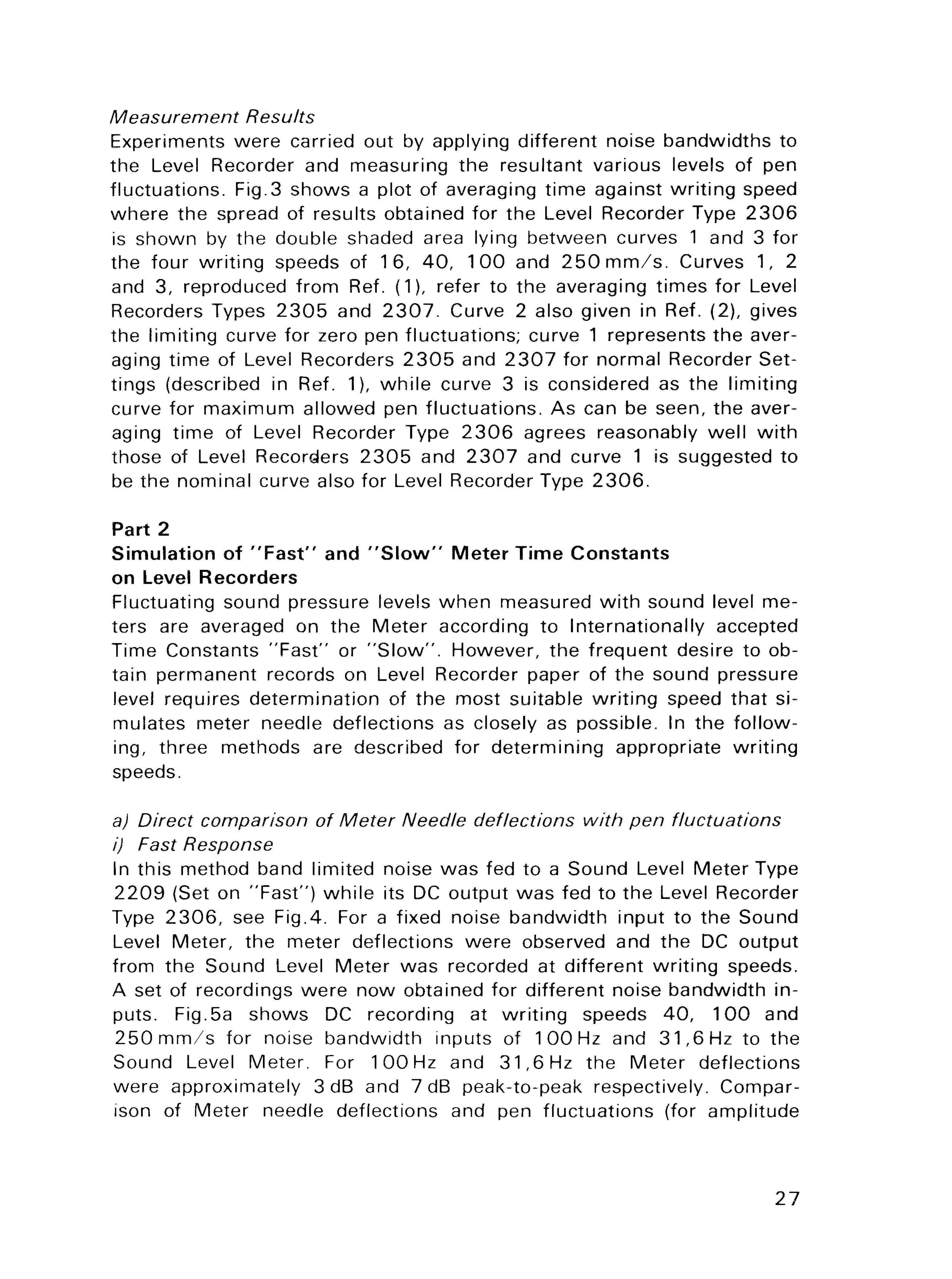
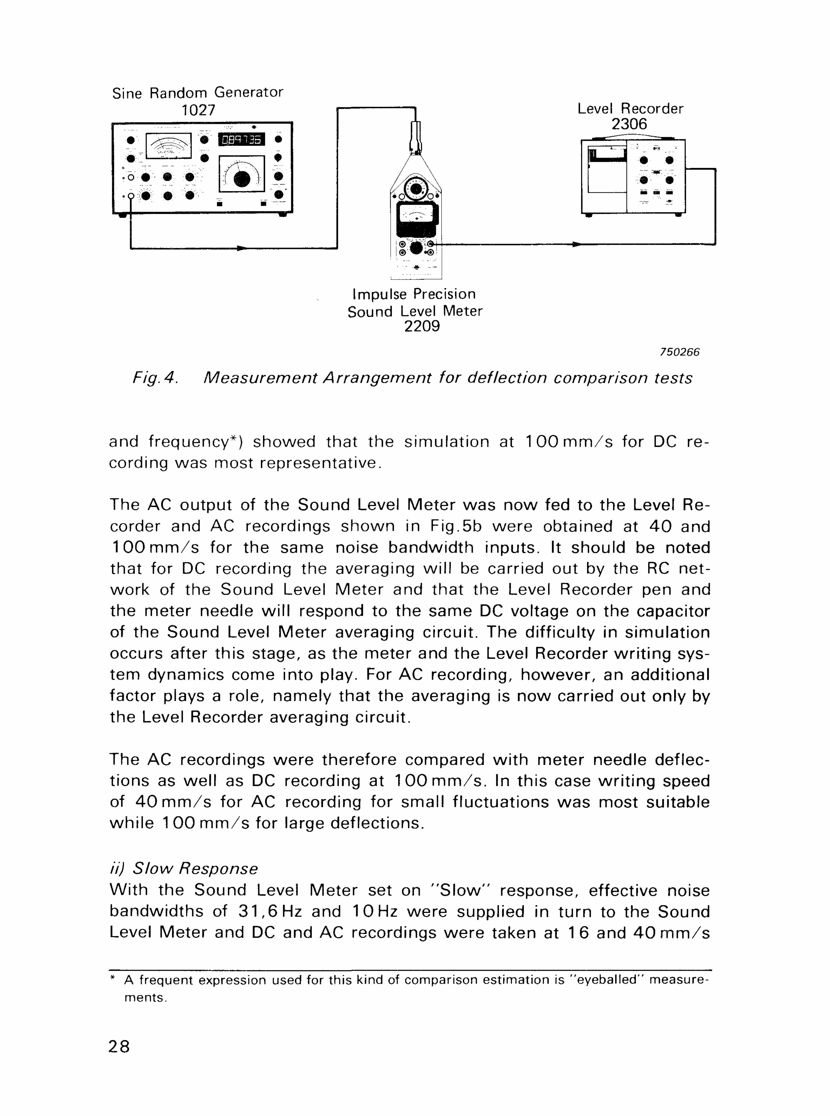
a) Direct comparison of Meter Needle deflections with pen fluctuations i) Fast Response In this method band l imited noise was fed to a Sound Level Meter Type 2 2 0 9 (Set on "Fast") wh i le its DC output was fed to the Level Recorder Type 2 3 0 6 , see Fig.4. For a fixed noise bandwidth input to the Sound Level Meter, the meter deflections were observed and the DC output from the Sound Level Meter was recorded at different wr i t ing speeds. A set of recordings were now obtained for different noise bandwidth in­puts. Fig.5a shows DC recording at wr i t ing speeds 4 0 , 100 and 2 5 0 m m / s for noise bandwidth inputs of 100 Hz and 31 ,6 Hz to the Sound Level Meter. For 100 Hz and 31 ,6 Hz the Meter deflections were approximately 3 dB and 7 dB peak-to-peak respectively. Compar­ison of Meter needle deflections and pen f luctuat ions (for amplitude

27

* * ^ \^ A^ ^_^ v ^

Fig. 4. Measurement Arrangement for deflection comparison tests

and frequency*) showed that the simulation at 1 0 0 m m / s for DC re­cording was most representative.

The AC output of the Sound Level Meter was now fed to the Level Re­corder and AC recordings shown in Fig.5b were obtained at 4 0 and 1 0 0 m m / s for the same noise bandwidth inputs. It should be noted that for DC recording the averaging wi l l be carried out by the RC net­work of the Sound Level Meter and that the Level Recorder pen and the meter needle wi l l respond to the same DC voltage on the capacitor of the Sound Level Meter averaging circuit. The difficulty in simulation occurs after this stage, as the meter and the Level Recorder wr i t ing sys­tem dynamics come into play. For AC recording, however, an additional factor plays a role, namely that the averaging is now carried out only by the Level Recorder averaging circuit.

The AC recordings were therefore compared wi th meter needle deflec­tions as wel l as DC recording at 1 0 0 m m / s . In this case wr i t ing speed of 4 0 m m / s for AC recording for small f luctuations was most suitable whi le 1 00 m m / s for large deflections.

ii) Slow Response With the Sound Level Meter set on " S l o w " response, effective noise bandwidths of 31 ,6 Hz and 10 Hz were supplied in turn to the Sound Level Meter and DC and AC recordings were taken at 16 and 4 0 m m / s

* A frequent expression used for this kind of comparison estimation is "eyebal led" measure­ments.

28

co C O

co

CO CD

v

O

C o

CO

CD CO

o C

c CD

I

CD

O

CO Co

o to CD

CO o CM

-ci

29

29

03 CO

o to

cb

"to CD

O

.O ■5?

CO

cb

CD

I

O

CD

o

CO

O

Q

O

CD

- —

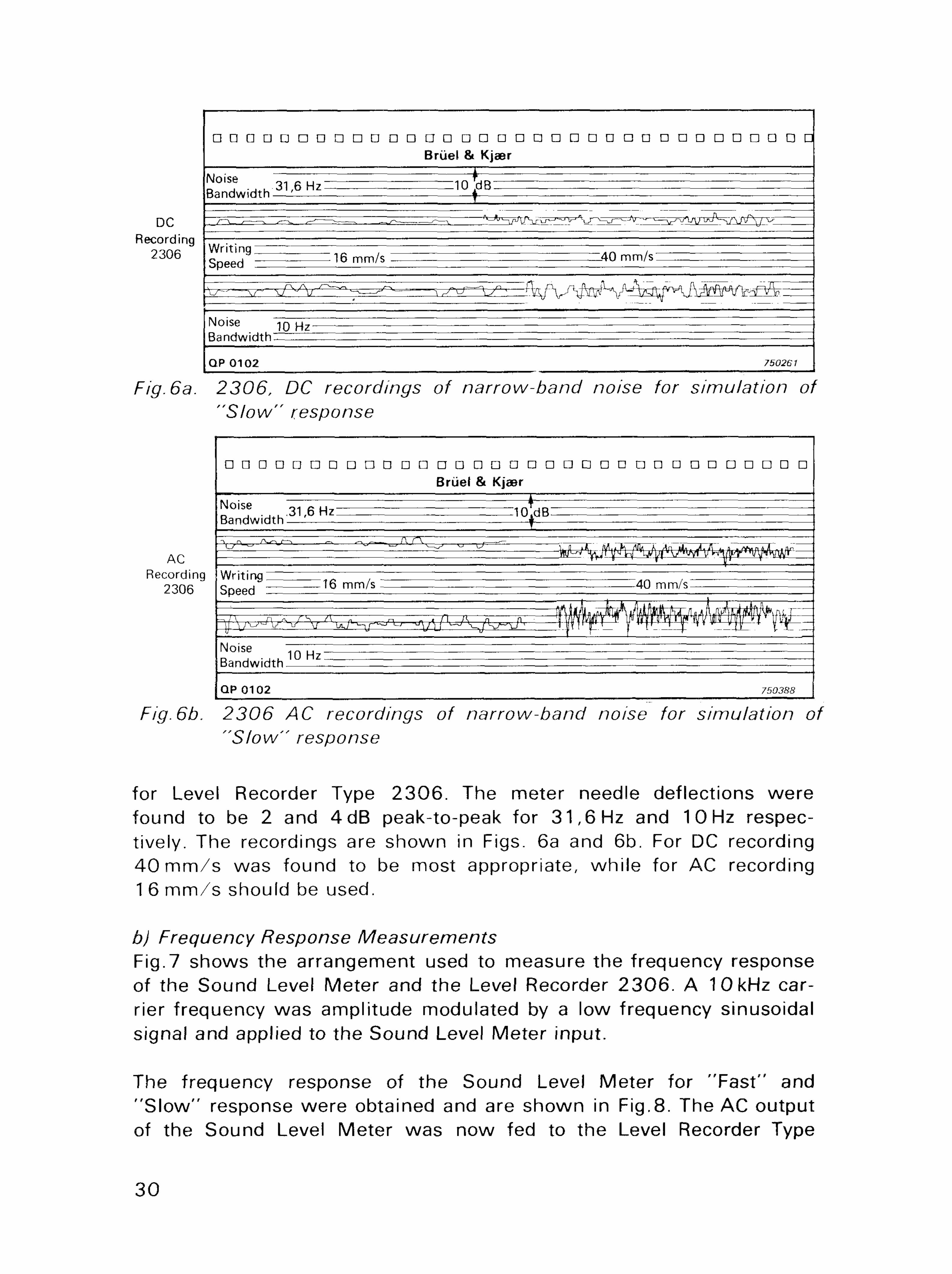
Fig.6a. 2306, DC recordings of narrow-band noise for simulation of "Slow" response

n n n D D n n D n D n a n a n D n D a a n n n n n D n n D n D D D Bruel & Kjaer

Bandwidth ———————- _ — -*— — — — — —

Recording Writing ^ ^ 7 ~ — -7^ 7 2 3 0 6 Speed = = = = ^ L 6 m m / s — — - - 40 mm/s _ — _ -

Noise 1 f 1 ■_. ~ " — ~ Bandwidth - — — ^ =

QP0102 750388 _ J

Fig.6b. 2306 AC recordings of narrow-band noise for simulation of "Slow" response

for Level Recorder Type 2 3 0 6 . The meter needle deflections were found to be 2 and 4 d B peak-to-peak for 31 ,6 Hz and 10 Hz respec­tively. The recordings are shown in Figs. 6a and 6b. For DC recording 4 0 m m / s was found to be most appropriate, wh i le for AC recording 1 6 m m / s should be used.

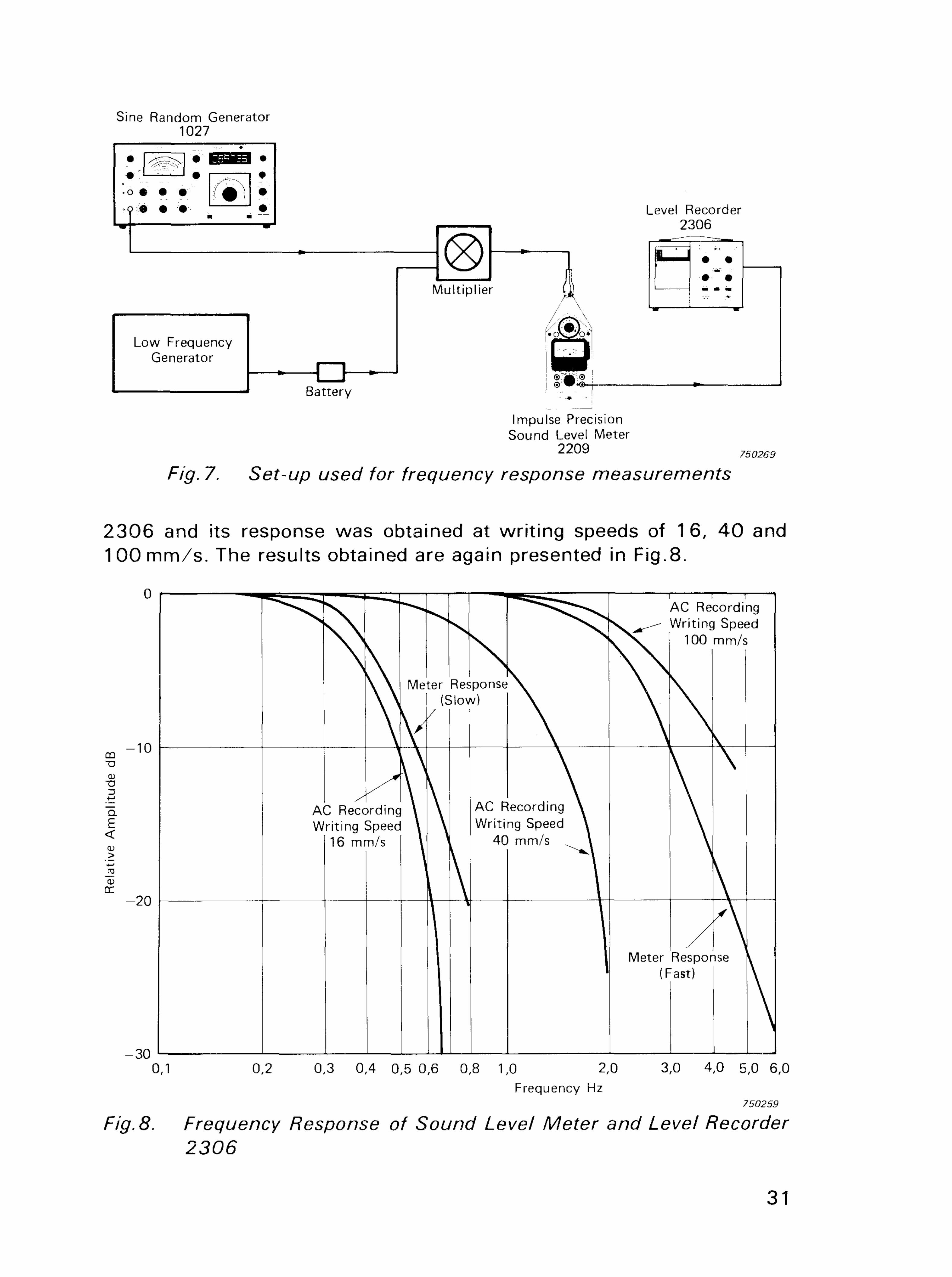
b) Frequency Response Measurements Fig.7 shows the arrangement used to measure the frequency response of the Sound Level Meter and the Level Recorder 2 3 0 6 . A 10 kHz car­rier frequency was ampli tude modulated by a low frequency sinusoidal signal and applied to the Sound Level Meter input.

The frequency response of the Sound Level Meter for "Fast " and " S l o w " response were obtained and are shown in Fig.8. The AC output of the Sound Level Meter was now fed to the Level Recorder Type

30

2209 750269

Fig. 7. Set-up used for frequency response measurements

2 3 0 6 and its response was obtained at wr i t ing speeds of 16, 4 0 and 1 00 m m / s . The results obtained are again presented in Fig.8.

^ ^ ^ ^ ^ ^ v - - - ^ ^ ^ ^ ^ ^ ^ ^ * ^ w AC Recording \ . \ ^ \ ^^^w t \ J * ^ - ~ Writing Speed

\ \ \ \ \ 10° mm/s

\ \ Meter Response \ \ \ \ \ I (Slow) \ \ \

€ AC Recording \ \ A C Recording \ \ J Writing Speed \ \ Writing Speed \ \ ^ 16 mm/s \ \ 4 0 m m / s -Oi \ 4 «■■■ B • ■ ^k

I 1 Meter Response y ' (Fast) \

-30 I ■ 1—■ 1 ' 1—LJJ—I 1 ■ 1 1—■—I L— 0,1 0,2 0,3 0,4 0,5 0,6 0,8 1,0 2,0 3,0 4,0 5,0 6,0

Frequency Hz 750259

Fig. 5. Frequency Response of Sound Level Meter and Level Recorder 2306

31

It can be seen that the Meter Response for "Fast" lies in-between the response for 4 0 m m / s and 1 00 m m / s for AC recordings. Therefore for "Fast" response it is suggested that for small deflections 4 0 m m / s should be used whi le 100 m m / s should be used for large deflections. For "S low" response 1 6 m m / s should be used.

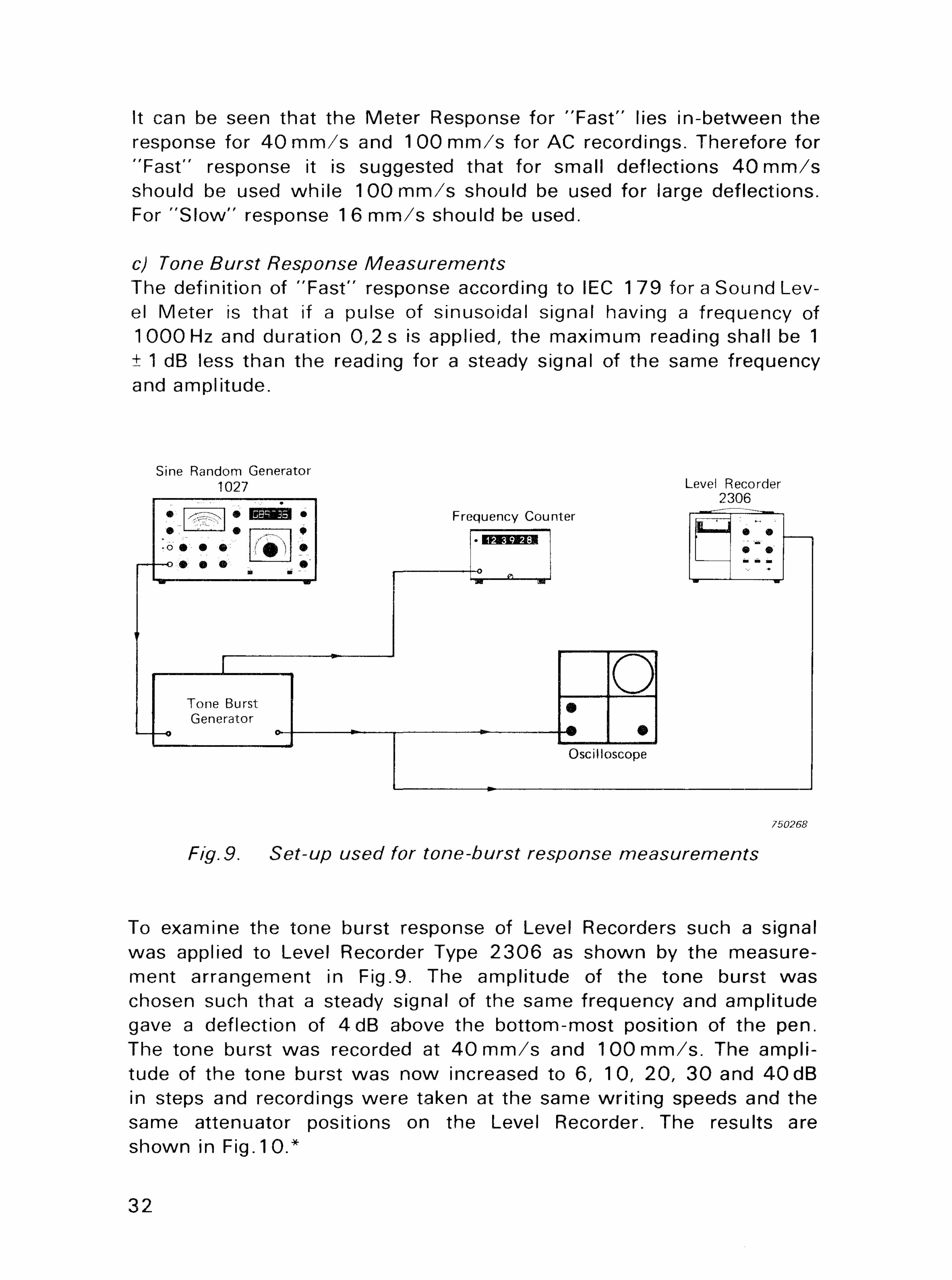
c) Tone Burst Response Measurements The definit ion of "Fast" response according to IEC 179 for a Sound Lev­el Meter is that if a pulse of sinusoidal signal having a frequency of 1000 Hz and duration 0,2 s is applied, the maximum reading shall be 1 ± 1 dB less than the reading for a steady signal of the same frequency and amplitude.

Fig. 9. Set-up used for tone-burst response measurements

To examine the tone burst response of Level Recorders such a signal was applied to Level Recorder Type 2 3 0 6 as shown by the measure­ment arrangement in Fig.9. The amplitude of the tone burst was chosen such that a steady signal of the same frequency and amplitude gave a deflection of 4dB above the bottom-most position of the pen. The tone burst was recorded at 4 0 m m / s and 100 m m / s . The ampli­tude of the tone burst was now increased to 6, 10, 20 , 30 and 4 0 dB in steps and recordings were taken at the same wr i t ing speeds and the same attenuator positions on the Level Recorder. The results are shown in Fig. 1 0.*

32

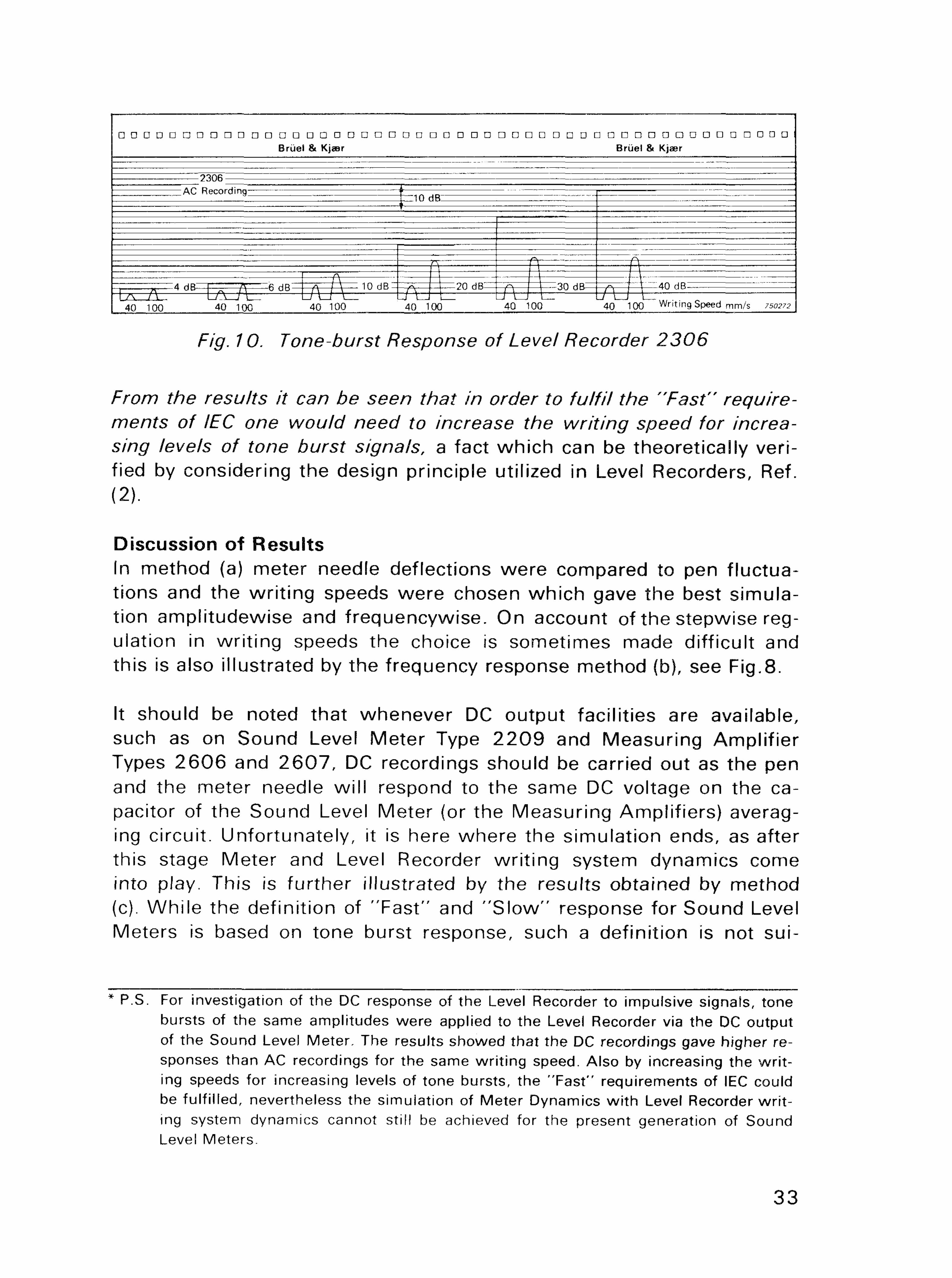
Fig. 10. Tone-burst Response of Level Recorder 2306

From the results it can be seen that in order to fulfil the "Fast" require­ments of IEC one would need to increase the writing speed for increa­sing levels of tone burst signals, a fact which can be theoretically veri­fied by considering the design principle utilized in Level Recorders, Ref. (2).

Discussion of Results In method (a) meter needle deflections were compared to pen f luctua­tions and the wr i t ing speeds were chosen which gave the best simula­tion amplitudewise and frequencywise. On account of the stepwise reg­ulation in wri t ing speeds the choice is sometimes made difficult and this is also il lustrated by the frequency response method (b), see Fig.8.

It should be noted that whenever DC output facilit ies are available, such as on Sound Level Meter Type 2 2 0 9 and Measuring Amplif ier Types 2 6 0 6 and 2 6 0 7 , DC recordings should be carried out as the pen and the meter needle wi l l respond to the same DC voltage on the ca­pacitor of the Sound Level Meter (or the Measuring Amplif iers) averag­ing circuit. Unfortunately, it is here where the simulation ends, as after this stage Meter and Level Recorder wri t ing system dynamics come into play. This is further il lustrated by the results obtained by method (c). Whi le the definit ion of "Fast" and " S l o w " response for Sound Level Meters is based on tone burst response, such a definit ion is not sui-

* P.S. For investigation of the DC response of the Level Recorder to impulsive signals, tone bursts of the same amplitudes were applied to the Level Recorder via the DC output of the Sound Level Meter. The results showed that the DC recordings gave higher re­sponses than AC recordings for the same wr i t ing speed. Also by increasing the wr i t ­ing speeds for increasing levels of tone bursts, the "Fast" requirements of IEC could be ful f i l led, nevertheless the simulation of Meter Dynamics wi th Level Recorder wr i t ­ing system dynamics cannot still be achieved for the present generation of Sound Level Meters.

33

34

CD co

CD

CO

o

■52

. |

CO

CD

c CO

I

O

CO

c: o CO

O

o Q

O CN

CO

CO

CD

CO

CO

z o ■■S

CO

.52

CO

I

O

CO

c:

o CO

t̂o­co" <o

to

oo

.5

to

O

CO

o CO

s ! CO

<*> Co

.1

O

co OS

. $

s ! CO

^ Co

35

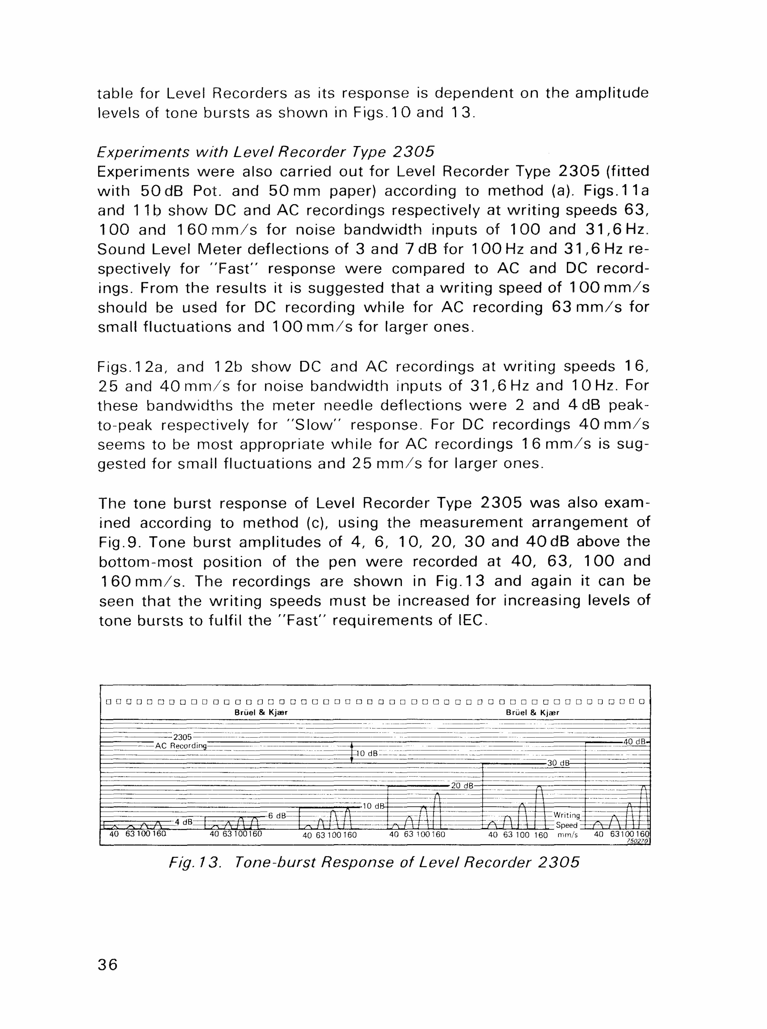
table for Level Recorders as its response is dependent on the amplitude levels of tone bursts as shown in Figs. 1 0 and 1 3.

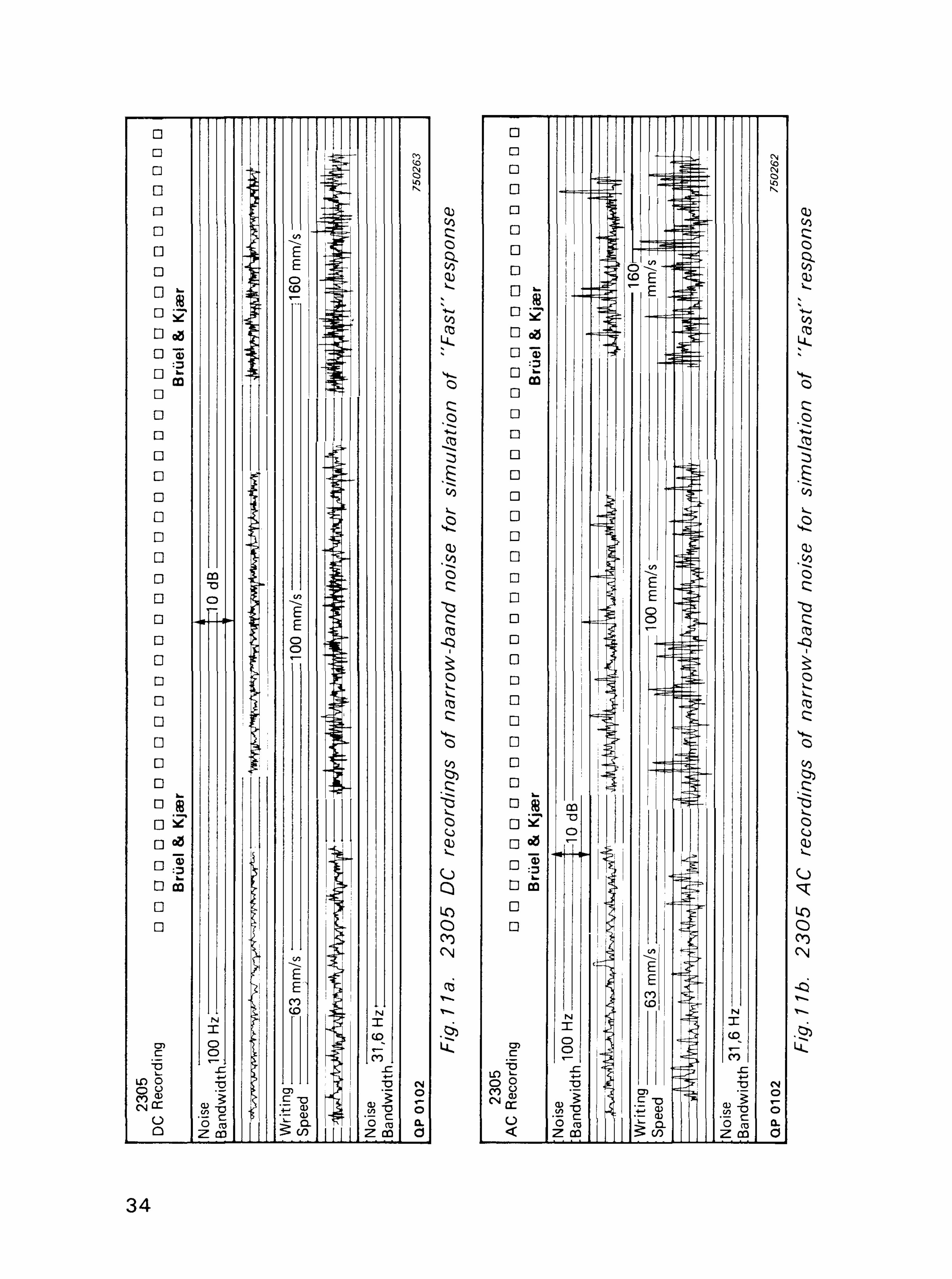
Experiments with Level Recorder Type 2305 Experiments were also carried out for Level Recorder Type 2 3 0 5 (fitted w i th 50dB Pot. and 50 mm paper) according to method (a). Figs. 11a and 1 1b show DC and AC recordings respectively at wr i t ing speeds 63 , 100 and 1 6 0 m m / s for noise bandwidth inputs of 100 and 31 ,6 Hz. Sound Level Meter deflections of 3 and 7 dB for 100 Hz and 31 ,6 Hz re­spectively for "Fast" response were compared to AC and DC record­ings. From the results it is suggested that a wr i t ing speed of 1 0 0 m m / s should be used for DC recording whi le for AC recording 63 m m / s for small f luctuations and 1 0 0 m m / s for larger ones.

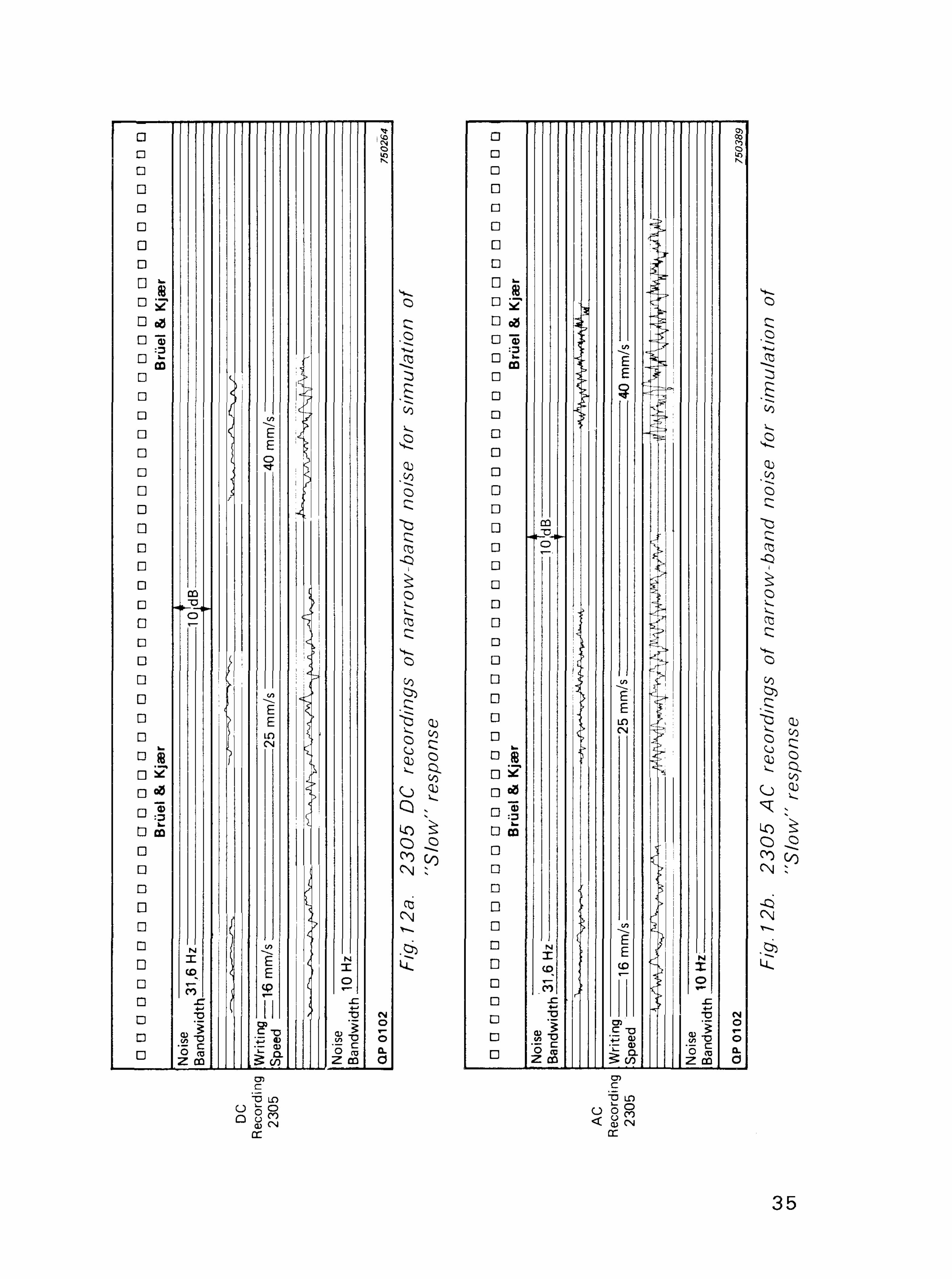
Figs. 12a, and 12b show DC and AC recordings at wr i t ing speeds 16, 25 and 40 m m / s for noise bandwidth inputs of 31 ,6 Hz and 10 Hz. For these bandwidths the meter needle deflections were 2 and 4 dB peak-to-peak respectively for " S l o w " response. For DC recordings 4 0 m m / s seems to be most appropriate whi le for AC recordings 1 6 m m / s is sug­gested for small f luctuations and 25 m m / s for larger ones.

The tone burst response of Level Recorder Type 2 3 0 5 was also exam­ined according to method (c), using the measurement arrangement of Fig.9. Tone burst amplitudes of 4, 6, 10, 20 , 30 and 4 0 d B above the bottom-most position of the pen were recorded at 4 0 , 63 , 100 and 1 60 m m / s . The recordings are shown in Fig. 13 and again it can be seen that the wr i t ing speeds must be increased for increasing levels of tone bursts to fulf i l the "Fast" requirements of IEC.

Fig. 13. Tone-burst Response of Level Recorder 2305

36

Conclusions The averaging times of Level Recorder Type 2 3 0 6 agree reasonably wel l w i th those of Level Recorders 2 3 0 5 and 2 3 0 7 , and curve 1 in Fig.3 is suggested to be the nominal curve also for Level Recorder Type 2306 .

For stationary random signals w i th small f luc tuat ions equivalent wr i t ­ing speeds on Level Recorders can be found that would simulate pen fluctuations w i th meter needle deflections of the present generation of Sound Level Meters both amplitudewise and frequencywise.

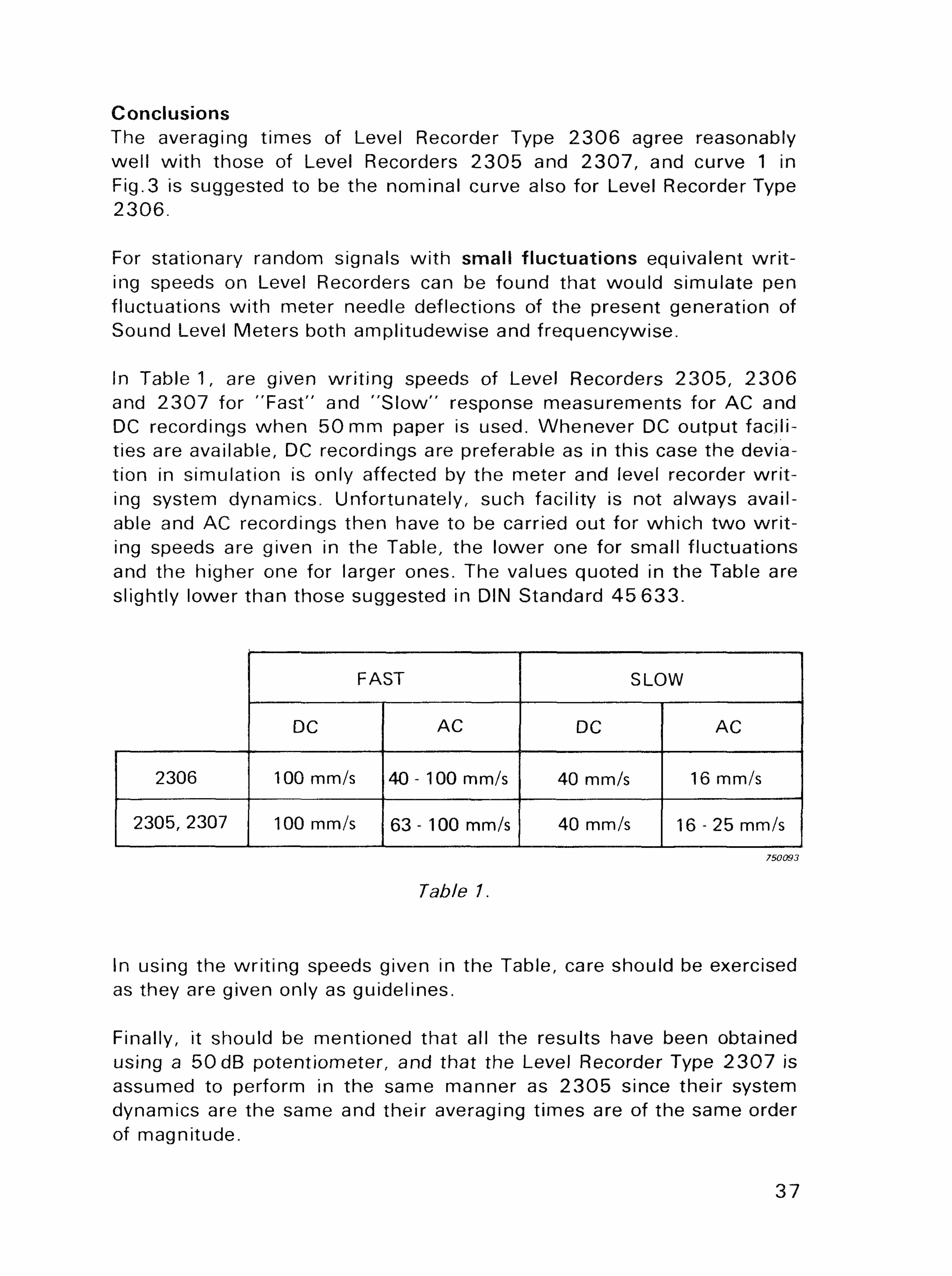
In Table 1 , are given wr i t ing speeds of Level Recorders 2 3 0 5 , 2 3 0 6 and 2 3 0 7 for "Fast" and " S l o w " response measurements for AC and DC recordings when 50 mm paper is used. Whenever DC output facji i-ties are available, DC recordings are preferable as in this case the devia­tion in simulation is only affected by the meter and level recorder wr i t ­ing system dynamics. Unfortunately, such facility is not always avail­able and AC recordings then have to be carried out for which two wr i t ­ing speeds are given in the Table, the lower one for small f luctuations and the higher one for larger ones. The values quoted in the Table are slightly lower than those suggested in DIN Standard 45 633 .

FAST SLOW

DC AC DC AC

2306 100 mm/s 40 - 100 mm/s 40 mm/s 16 mm/s

2305,2307 100 mm/s 63-100 mm/s 40 mm/s 16-25 mm/s

750093

Table 7.

In using the wr i t ing speeds given in the Table, care should be exercised as they are given only as guidelines.

Finally, it should be mentioned that all the results have been obtained using a 5 0 d B potentiometer, and that the Level Recorder Type 2 3 0 7 is assumed to perform in the same manner as 2 3 0 5 since their system dynamics are the same and their averaging times are of the same order of magnitude.

37

FAST SLOW

DC AC DC AC

2306 100 mm/s 40-100 mm/s 40 mm/s 16 mm/s

2305, 2307 100 mm/s 63- 100 mm/s 40 mm/s 16 -25 mm/s

Table 7.

750O93

References 1. H. P. OLESEN and Measurements of Averaging Times of

K. ZAVERI Level Recorders Types 2 3 0 5 and 2 3 0 7 . Bruel & Kjaer Technical Review No. 1 — 1974 .

2. JENS T. BROCH and Effective Averaging Time of the Level Re-CARL G. WAHRMANN corder Type 2 3 0 5 . Bruel & Kjser Techni­

cal Review No. 1 — 1 9 6 1 .

3. JULIUS S. BENDAT and Random Data: Analysis and Measure-ALLAN G. PIERSOL ment Procedures, Wiley-lnterscience

1 9 7 1 .

38

News from the Factory

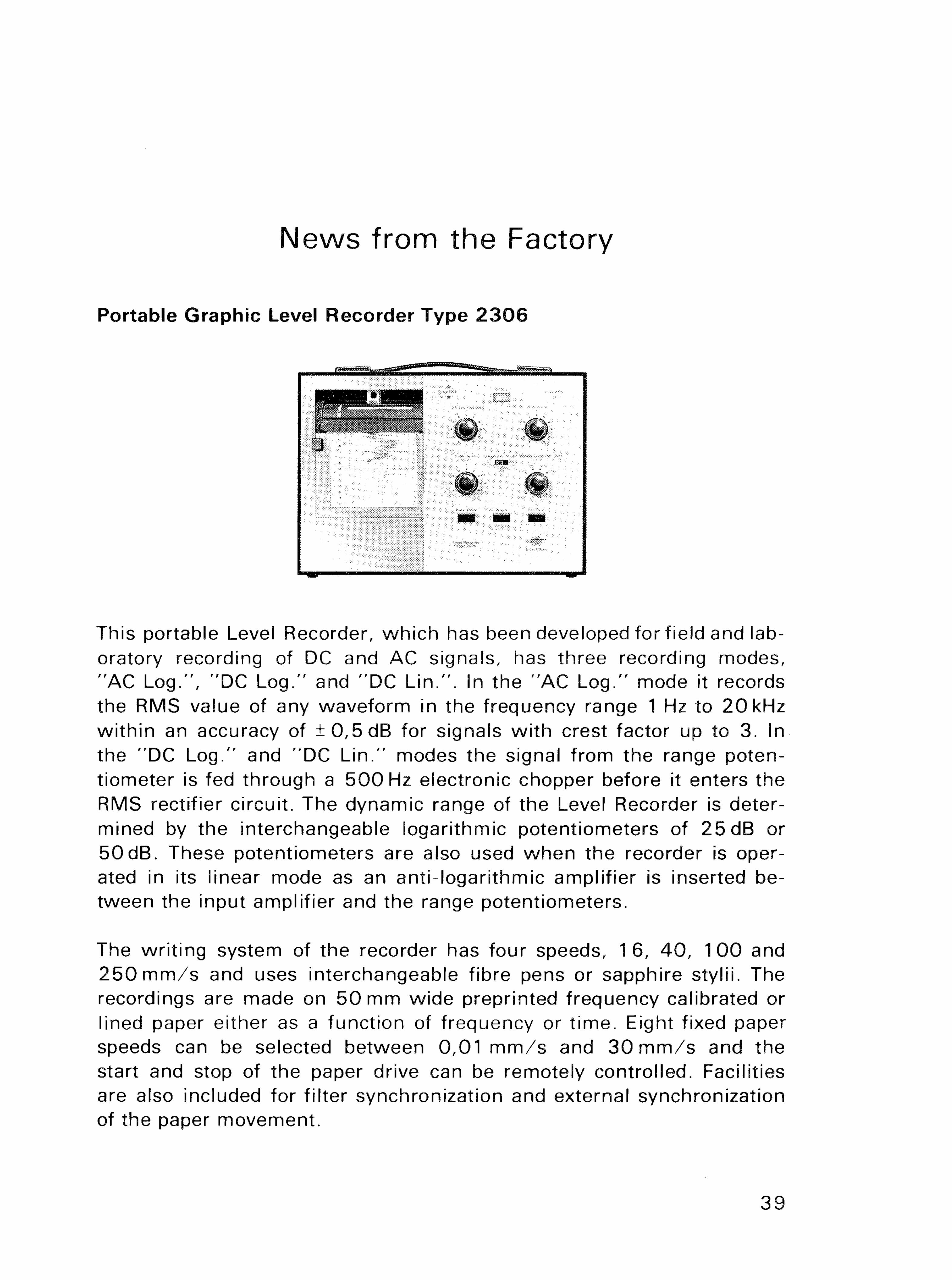
Portable Graphic Level Recorder Type 2 3 0 6

This portable Level Recorder, which has been developed for field and lab­oratory recording of DC and AC signals, has three recording modes, "AC Log." , "DC Log." and "DC L in . " . In the "AC Log." mode it records the RMS value of any waveform in the frequency range 1 Hz to 20 kHz wi th in an accuracy of ± 0 , 5 d B for signals w i th crest factor up to 3. In the "DC Log." and "DC L in . " modes the signal from the range poten­tiometer is fed through a 5 0 0 Hz electronic chopper before it enters the RMS rectifier circuit. The dynamic range of the Level Recorder is deter­mined by the interchangeable logarithmic potentiometers of 25 dB or 5 0 d B . These potentiometers are also used when the recorder is oper­ated in its linear mode as an anti- logarithmic amplifier is inserted be­tween the input amplifier and the range potentiometers.

The wri t ing system of the recorder has four speeds, 16, 4 0 , 100 and 2 5 0 m m / s and uses interchangeable fibre pens or sapphire styli i . The recordings are made on 50 mm wide preprinted frequency calibrated or lined paper either as a function of frequency or t ime. Eight fixed paper speeds can be selected between 0,01 m m / s and 3 0 m m / s and the start and stop of the paper drive can be remotely controlled. Facilities are also included for filter synchronization and external synchronization of the paper movement.

39

The power for driving the recorder can be supplied either from dry cells, rechargeable NiCd-batteries, from the mains via the plug-in Power Supply Type 2 8 0 8 or from an ordinary 1 2 V automobile battery. A built- in miniature meter on the front panel is also provided for moni­toring the supply voltage.

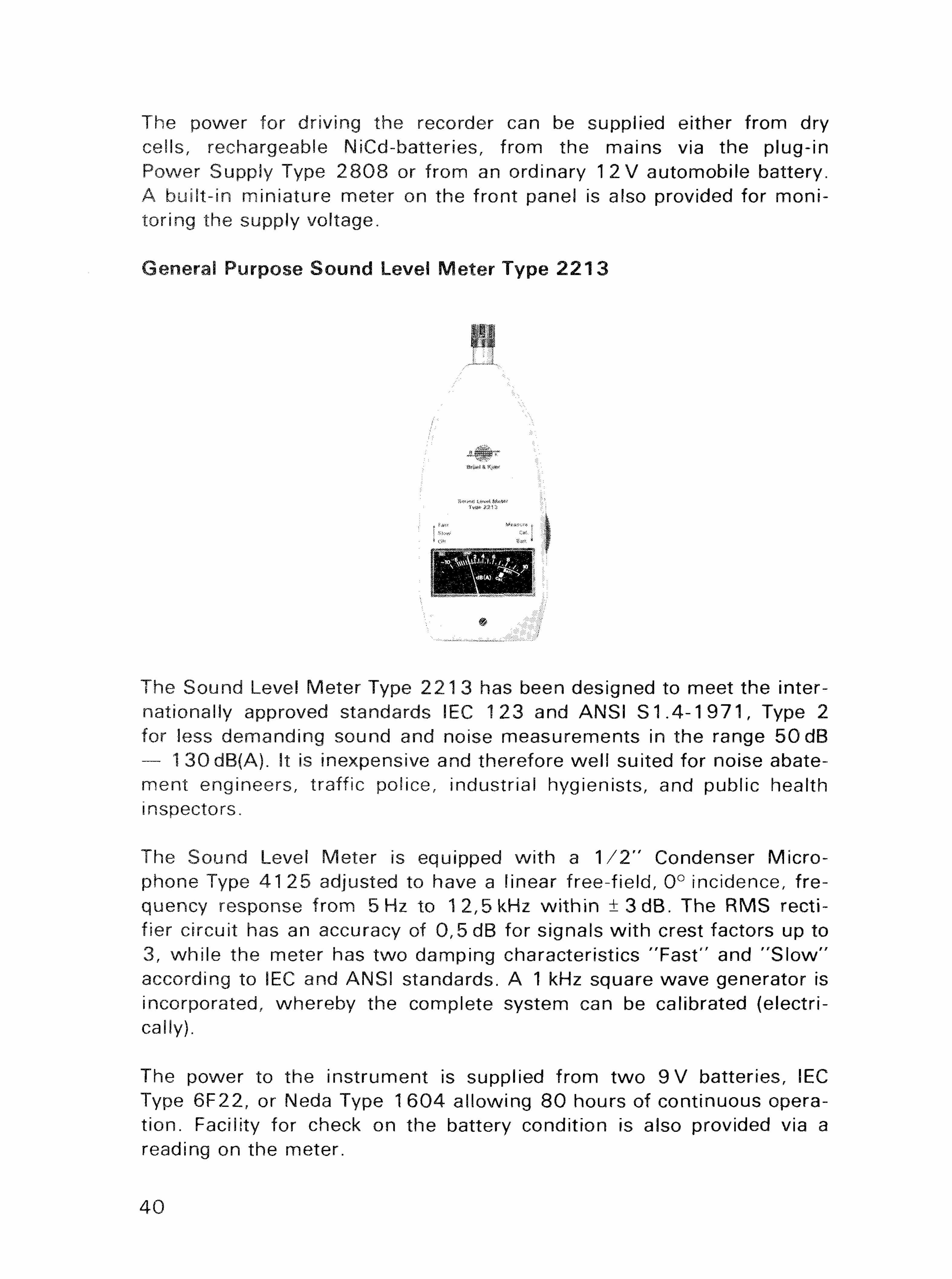
General Purpose Sound Level Meter Type 2 2 1 3

The Sound Level Meter Type 221 3 has been designed to meet the inter­nationally approved standards IEC 123 and ANSI S1.4-1 9 7 1 , Type 2 for less demanding sound and noise measurements in the range 50 dB — 1 30dB(A)„ It is inexpensive and therefore wel l suited for noise abate­ment engineers, traffic police, industrial hygienists, and public health inspectors.

The Sound Level Meter is equipped wi th a 1 / 2 " Condenser Micro­phone Type 4 1 2 5 adjusted to have a linear free-field, 0° incidence, fre­quency response from 5 Hz to 12,5 kHz wi th in ± 3 d B . The RMS recti­fier circuit has an accuracy of 0 ,5dB for signals w i th crest factors up to 3, whi le the meter has two damping characteristics "Fast" and " S l o w " according to IEC and ANSI standards. A 1 kHz square wave generator is incorporated, whereby the complete system can be calibrated (electri­cally),

The power to the instrument is supplied from two 9 V batteries, IEC Type 6F22, or Neda Type 1 6 0 4 al lowing 8 0 hours of continuous opera­t ion. Facility for check on the battery condition is also provided via a reading on the meter.

40

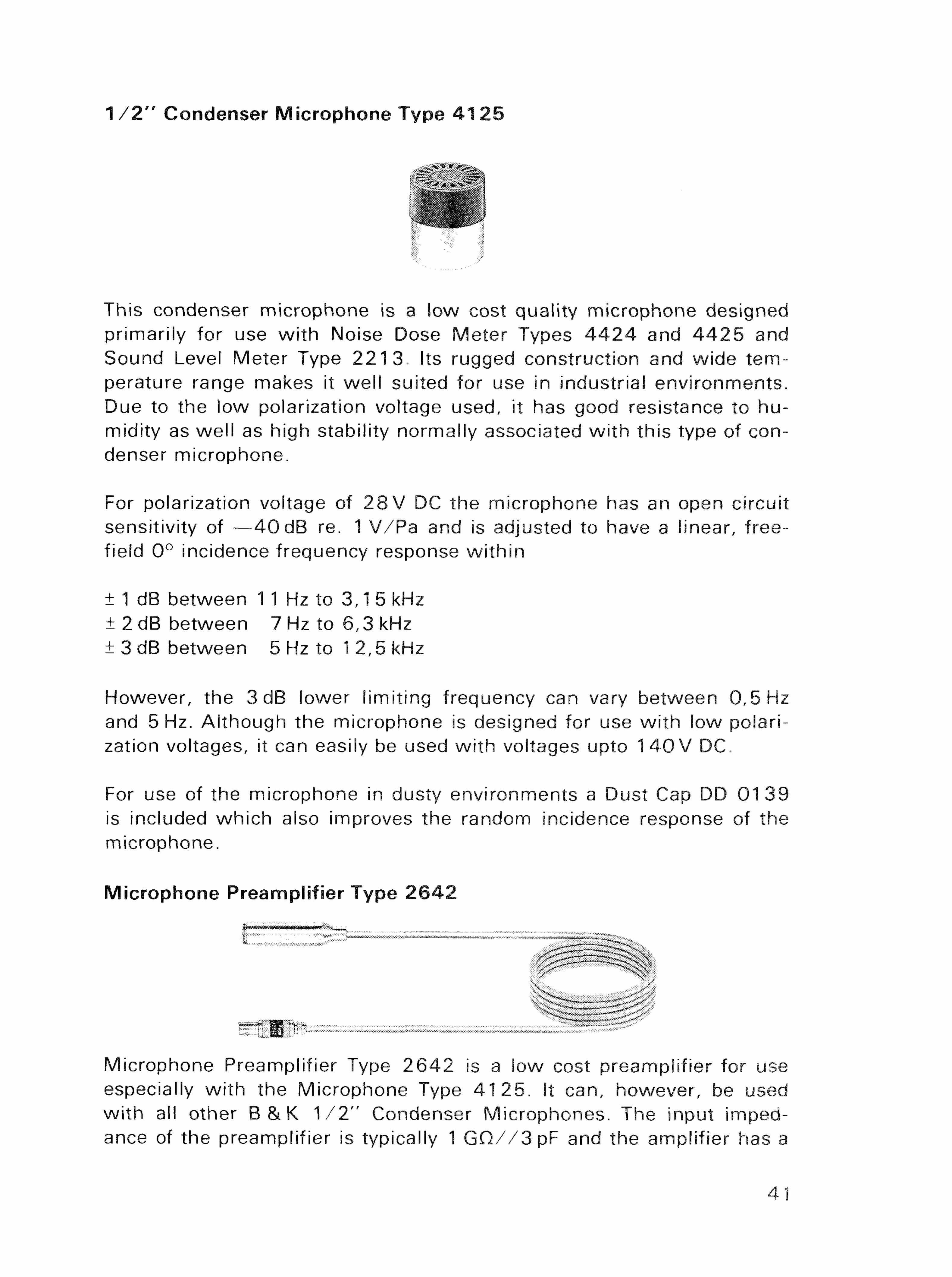
1 / 2 " Condenser Microphone Type 41 25

This condenser microphone is a low cost quality microphone designed primarily for use w i th Noise Dose Meter Types 4 4 2 4 and 4 4 2 5 and Sound Level Meter Type 2213= Its rugged construction and wide tem­perature range makes it wel l suited for use in industrial environments. Due to the low polarization voltage used, it has good resistance to hu­midity as wel l as high stability normally associated w i th this type of con­denser microphone.

For polarization voltage of 2 8 V DC the microphone has an open circuit sensitivity of — 4 0 dB re. 1 V /Pa and is adjusted to have a linear, free-field 0° incidence frequency response wi th in

± 1 dB between 1 1 Hz to 3,1 5 kHz ± 2 dB between 7 Hz to 6,3 kHz ± 3 dB between 5 Hz to 1 2,5 kHz

However, the 3 dB lower l imit ing frequency can vary between 0,5 Hz and 5 Hz. Although the microphone is designed for use w i th low polari­zation voltages, it can easily be used wi th voltages upto 1 40 V DC.

For use of the microphone in dusty environments a Dust Cap DD 0 1 3 9 is included which also improves the random incidence response of the microphone.

Microphone Preamplif ier Type 2 6 4 2

Microphone Preamplifier Type 2 6 4 2 is a low cost preamplifier for use especially wi th the Microphone Type 4 1 2 5 . It can, however, be used wi th all other B & K 1 / 2 " Condenser Microphones. The input imped­ance of the preamplifier is typically 1 G O / / 3 p F and the amplifier has a

41

linear frequency response from 20 Hz to 20 kHz wi th in ± 1 dB wi th a transducer capacitance of 1 5 pF connected to the input.

The power for the preamplifier and polarization voltage for the micro­phone can be supplied either from a Microphone Power Supply Type 2 8 1 0 or from B & K Spectrometers, Analyzers, and Measuring Ampl i f i ­ers via the adaptor JP 0 7 0 8 .

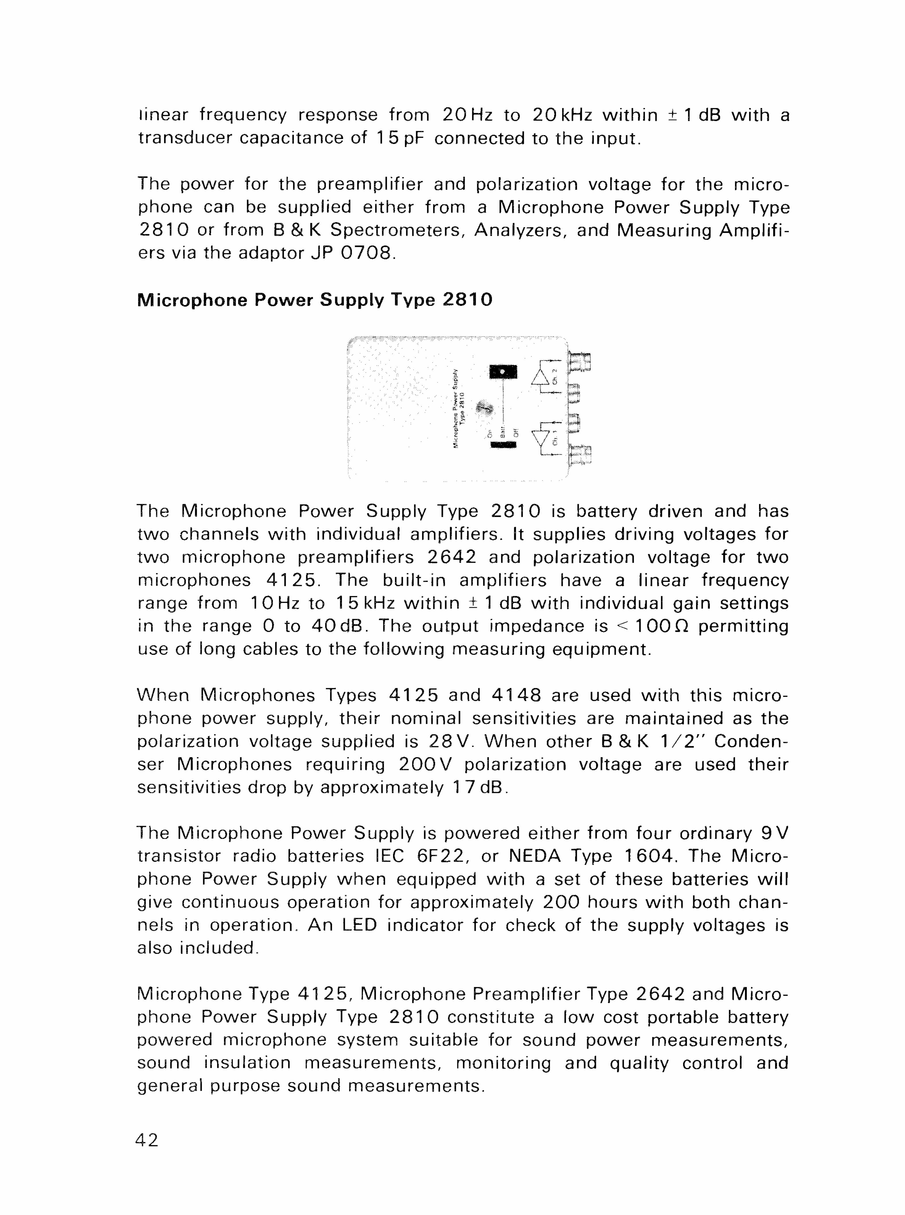
Microphone Power Supply Type 2 8 1 0

The Microphone Power Supply Type 2 8 1 0 is battery driven and has two channels wi th individual amplif iers. It supplies driving voltages for two microphone preamplifiers 2 6 4 2 and polarization voltage for two microphones 4 1 2 5 . The built- in amplifiers have a linear frequency range from 1 0 Hz to 15 kHz wi th in ± 1 dB wi th individual gain settings in the range 0 to 4 0 d B . The output impedance is < 1 0 0 O permitt ing use of long cables to the fol lowing measuring equipment.

When Microphones Types 4 1 2 5 and 4 1 4 8 are used wi th this micro­phone power supply, their nominal sensitivities are maintained as the polarization voltage supplied is 2 8 V . When other B & K 1 / 2 " Conden­ser Microphones requiring 2 0 0 V polarization voltage are used their sensitivities drop by approximately 1 7 dB.

The Microphone Power Supply is powered either from four ordinary 9 V transistor radio batteries IEC 6F22, or NEDA Type 1604 . The Micro­phone Power Supply when equipped wi th a set of these batteries will give continuous operation for approximately 2 0 0 hours wi th both chan­nels in operation. An LED indicator for check of the supply voltages is also included.

Microphone Type 41 25 , Microphone Preamplifier Type 2 6 4 2 and Micro­phone Power Supply Type 2 8 1 0 constitute a low cost portable battery powered microphone system suitable for sound power measurements, sound insulation measurements, monitoring and quality control and general purpose sound measurements.

42

P R E V I O U S L Y I S S U E D N U M B E R S O F B R U E L & K J / E R T E C H N I C A L R E V I E W

(Continued from cover page 2)

1 1973 Calibration of Hydrophones. The Measurement of Reverberation Characteristics. Adaptation of Frequency Analyzer Type 2107 to Automated 1/12 Octave Spectrum Analysis in Musical Acoustics. Bekesy Audiometry with Standard Equipment.

4 1972 Measurement of Elastic Modulus and Loss Factor of Asphalt. The Digital Event Recorder Type 7502. Determination of the Radii of Nodal Circles on a Circular Metal Plate, New Protractor for Reverberation Time Measurements.

3-1972 Thermal Noise in Microphones and Preamplifiers, High Frequency Response of Force Transducers. Measurement of Low Level Vibrations in Buildings. Measurement of Damping Factor Using the Resonance Method.

2-1972 RMS-Rectifiers. Scandiavian Efforts to Standardize Acoustic. Response in Theaters and Dubbing Rooms. Noise Dose Measurements.

1-1972 Loudness Evaluation of Acoustic Impulses. Computer Programming Requirements for Acoustic Measurements. Computer Interface and Software for On-Line Evaluation of Noise Data. Evaluation of Noise Measurements in Algol-60.

S P E C I A L T E C H N I C A L L I T E R A T U R E

As shown on the back cover page Bruel & Kjaer publish a variety of technical literature which can be obtained free of charge, The following literature is presently available:

Mechanical Vibration and Shock Measurements (English, German, Russian) Acoustic Noise Measurements (English, Russian), 2. edifon Architectural Acoustics (English) Power Spectral Density Measurements and Frequency Analysis (English) Standards, formulae and charts (English) Catalogs (several languages) Product Data Sheets (English, German, French, Russian)

Furthermore, back copies of the Technical Review can be supplied as shown in the list above. Older issues may be obtained provided they are still in stock.

PRINTED IN OFNMARr < LAR5FN &■ S0N A /S 0K-28A0 S0BORG