Pretrial Negotiations Under Optimism

Shoshana Vasserman

Harvard Economics Department

svasserman@fas.harvard.edu

Muhamet Yildiz

MIT Economics Department

myildiz@mit.edu ∗

August 8, 2018

Abstract

We develop a tractable and versatile model of pretrial negotiation in which the

negotiating parties are optimistic about the judge’s decision and anticipate the possible

arrival of public information about the case prior to the trial date. The parties will

settle immediately upon the arrival of information. However, they may agree to settle

prior to an arrival as well. We derive the settlement dynamics prior to an arrival and

show that negotiations result in either immediate agreement, a weak deadline effect

— settling at a particular date before the deadline, a strong deadline effect — settling

at the deadline, or impasse, depending on the level of optimism. We show that the

distribution of settlement times has a U-shaped frequency and a convexly increasing

hazard rate with a sharp increase at the deadline, replicating stylized facts about such

negotiations.

∗We thank Kathryn Spier and our anonymous referees for their detailed comments. We also thank Jim

An for his assistance in connecting our model to existing legal precedent and common legal practice. Finally,

we thank the participants of the Harvard Law and Economics Seminar and the ALEA 2016 annual meeting

for their comments.

1 Introduction

Costly settlement delays and impasse are common in pretrial negotiations. Whereas only

about 5% of the cases in the United States go to trial, the parties settle only after long, costly

delays.1 Excessive optimism has been recognized as a major cause of delay and impasse in

pretrial negotiations, especially when the optimistic parties learn about the strength of their

cases over time. In this article, we develop a tractable model of pretrial negotiations in which

optimistic negotiators may receive public information relating to the outcomes of their cases

as negotiations progress. We determine the dates at which a settlement is possible and

obtain sharp characterizations of patterns of behavior as outputs of our model. Our analysis

predicts some well-known stylized facts and also makes a few novel predictions.

Optimism and self-serving biases are commonly observed, even among highly experienced

litigators. In an empirical study of lawyers’ aptitude in accurately predicting the outcomes

of their cases, Goodman-Delahunty et al. (2010) surveyed a cross section of lawyers across

the United States, asking for their assessments of the probability that they would meet a

self-identified minimum goal for a case set for trial.2 Comparing the surveyed responses with

realized case outcomes, the authors found that even highly experienced lawyers (with 10+

years of experience) overestimated their probability of success by 9% on average.3

Moreover, although the probability of success reported to Goodman-Delahunty, et al. var-

ied between optimism and pessimism, there was not a strong relationship between optimism

and success. Whereas reported confidence levels (interpreted as subjective probabilities of

success) varied from around 20% to around 90%, the actualized success rates were around

50% for most confidence levels. This suggests that the lawyers’ confidence was, at least

in large part, independent of superior knowledge or understanding. Note that this finding

1Average settlement delay in malpractice insurance cases is reported to be 1.7 years (Watanabe (2006)).

The legal cost of settlement delays in high-stake cases are sometimes on the order of tens of millions of

dollars. In the well-known case of Pennzoil v. Texaco, the legal expenses were several hundreds of millions

of dollars, and the case was settled for 3 billion dollars after a long litigation process (see Mnookin and

Wilson (1989) and Lloyd (2004)). In commercial litigation, ongoing litigation also have indirect costs due to

uncertainty, delayed decisions, missed business opportunities, and suppressed market valuation, and these

costs may dwarf the legal expenses above.2See Loftus and Wagenaar (1988) and Malsch (1990) for earlier, similar analyses and Babcock and Loewen-

stein (1997) for a review of the literature on the empirical evidence for excessive optimism among negotiators.3Highly experienced lawyers reported a 63% probability of success on average, but only 55% achieved

their goals. Furthermore there was almost no difference between lawyers who were highly experienced (with

10+ years of experience) and the rest of the sample, which predicted 64% probability of success on average,

but had a 54% rate of goal achievement.

1

is inconsistent with a model of asymmetric information with a common prior, as such a

model would predict that confidence rates are consistent estimators of the rate of success on

average.

A number of experimental studies investigating self-serving biases in negotiations have

found persistent evidence of overconfidence across contexts and treatments. In a classic

experiment on optimism in final offer arbitration, Neale and Bazerman (1983) found that

subjects reported a probability of 68%, on average, when asked the likelihood with which

they believed that their offer would be accepted. This finding suggests that the subjects

did not have a common prior, as a common prior would imply the subjects should report a

probability of 50% on average—even after counting for selection bias.4

In this article, we build on the canonical pretrial negotiation framework to construct a

tractable model of pretrial negotiations in the presence of optimism. A plaintiff has filed a

case against a defendant, and they negotiate over an out-of-court settlement. At each date,

one party is randomly selected as a proposer; the proposer proposes a settlement amount

and the other party accepts or rejects. If the parties cannot settle by a given deadline, a

judge decides whether the defendant is liable. If the judge determines that the defendant

is liable, then the defendant pays a fixed amount J to the plaintiff; otherwise, he does not

pay anything. Delays are costly, in that each party pays a daily fee until the case is closed

and pays an additional cost if the case goes to trial. Unlike in the standard model, we

assume that the plaintiff assigns a higher probability to the defendant’s being found liable

in court than the defendant does; the difference between the two probabilities is the level of

optimism, denoted by y. For example, in Neale and Bazerman experiment, we would have

y = 2× 0.68− 1 = 0.36.

In our baseline model, we further assume that as time passes, the negotiating parties may

learn the strength of their respective cases by observing the arrival of new public information:

a single decisive piece of evidence that arrives with a fixed probability at each date, revealing

what the judge will decide. For example, in a securities fraud case, the negotiating parties

might anticipate evidence in the form of a contested internal memorandum that conclusively

sheds light on the corporate directives in question. Note that, for consistency, the probability

that the evidence would reveal a verdict in favor of the plaintiff (that is, a verdict that finds

the defendant liable) upon arrival is equal to the probability that the court would find in

favor of the plaintiff at the trial date, and hence the level of optimism about the nature of the

4To put this in context, if both the plaintiff and defendant believe that they will win with 68% probability,

then the divergence between the parties’ expectations is 2× 0.68− 1 = 0.36: the defendant believes that the

plaintiff overestimates her chances of success with 36% and vice versa.

2

information is also y. It is also worthwhile to emphasize that our baseline model assumes the

American Rule: each party incurs its own legal costs regardless of the outcome. Accordingly,

the plaintiff can withdraw her case at any time, and she cannot commit to continue pursuing

her case once it is revealed that the court will find in favor of the defendant.

The basic dynamics and the logic of delay in our model are as follows. After the arrival of

information, our model is identical to the standard bilateral bargaining model as in Bebchuk

(1996), and the parties agree immediately. The settlement amount depends on the nature

of the information. If the information reveals a verdict in favor of the plaintiff, a settlement

amount S is determined by splitting the savings from negotiation and litigation costs accord-

ing to the probability of making an offer for each party, which reflects that party’s bargaining

power in the standard model. If the information reveals a verdict in favor of the defendant,

then the settlement amount is zero. As S is non-negative, the players are optimistic about

the settlement amount after an arrival of information in equilibrium, and so, the difference

between the expected settlements after an information arrival is yS. Such optimism turns

out to be the main force towards a delay. In equilibrium, the parties strategically settle at

a given date without an information arrival if and only if the expected benefit from waiting

for yS through a future arrival of information is lower than the total cost of waiting. Hence,

we can determine the dynamics of strategic settlement by simply analyzing the settlement

amount S in the standard model.

The resulting pattern of behavior relies heavily on which party has the stronger bargaining

position. When the plaintiff has more bargaining power, S is an increasing function of the

remaining time until the court date, as the plaintiff gets some of the defendant’s cost savings

in the settlement. Hence, the incentive for delay increases as negotiations get farther from

the deadline. This results in a sharp prediction for the timing of the settlement. For high

values of optimism y, the players never settle strategically. They go to trial if information

does not arrive, no matter how far the trial date is. We call such an outcome impasse. For

intermediate values of optimism y, the players wait for an information arrival until the last

possible day for settlement, and strategically settle at the deadline. Such an agreement on

the steps of the courthouse is commonly observed in real-world negotiations and is referred

to as the deadline effect in the literature, as we discuss below. For low values of optimism,

equilibrium is characterized by a weaker version of the deadline effect: the parties wait until

a fixed number of days before the deadline to settle strategically. We define this as a weak

deadline effect.

If the defendant has stronger bargaining power than the plaintiff, then S is a decreasing

3

function of the time remaining until the deadline. In this case, the incentive to delay decreases

the farther away that the deadline is. In equilibrium, the parties strategically settle either

at the beginning or at the deadline, but never in between. Then, except for a settlement

due to information arrival, the only possible outcomes are: immediate agreement (for low

values of y or long deadlines), the deadline effect (for intermediate values of optimism) and

impasse (for high values of optimism).

Our model leads to sharp empirical predictions on the distribution of settlement times,

which is a combination of settlement due to an information arrival and strategic settlement.

There are point masses at the beginning and at the deadline—due to immediate agreement

and the deadline effect, respectively. In between, the overall frequency of settlements is

decreasing, yielding a U-shaped pattern. This is in line with empirical regularities. The

frequency of settlements decreases in the duration of negotiations (e.g. see Kessler (1996)),

but a significant number of cases settle at the deadline in studies that keep track of the

trial date. For example, Williams (1983) reports that 70% of civil cases in Arizona were

settled within 30 days of the trial date and 13% were settled on the trial date itself. A

U-shaped distribution of settlements also arises in some bargaining models with incomplete

information (Spier (1992) and Fanning (2016)). A more subtle parameter that is considered

in the empirical literature is the hazard rate of settlement, which measures the frequency

of settlements among cases that are ongoing. The hazard rate in our model is increasing

and convex—with a point mass at each end. The empirical studies that we are aware of are

mixed: Fournier and Zuehlke (1996) estimates a convexly increasing hazard rate as in here,

whereas Kessler (1996) reports a mildly decreasing hazard rate.

Our model is highly versatile and can be adapted to a variety of different environments.

To illustrate this, we study the reform of switching from the American Rule to the English

Rule. As in our baseline model, the American Rule, which is used in most of the United

States, requires each party to pay its own legal costs regardless of the outcome of the trial.

The English Rule, which is used in most of England and Canada, requires that the loser of

the trial pay all of the legal fees incurred in relation to the case if a case reaches trial. As

each rule has widespread use, the merits of imposing one over the other in different situations

is widely debated among policy makers. For example, whereas federal law provides for fee

shifting – typically to benefit plaintiffs in civil cases relating to civil rights5 – courts may

exercise discretion to allow defendants to recover costs under certain fee-shifting statutes

if the plaintiff’s claim was ”frivolous, unreasonable, or groundless.”6 Furthermore, recent

5See, for example, 42 U.S.C. § 1981, 28 U.S.C. § 2412, 42 U.S.C. § 6104(e)(1).6CRST Van Expedited, Inc. v. E.E.O.C., 136 S. Ct. 1642, 1652 (2016) (citing Christiansburg Garment

4

supreme court rulings have lowered the threshold for substantiating fee-shifting under the

Patent Act, making it easier for the winning party to sue to recover costs from the loser, as

would be the case under the English Rule.7

We show that under the English Rule, there is more disagreement and there are longer

delays among the cases that do settle. Thus, litigation is longer and costlier overall. The

logic of our result is straightforward. In our model, switching from the American Rule to the

English Rule is mathematically equivalent to adding to the judgment amount J , the total

costs C incurred—both to be paid by the loser under the English Rule. Such an increase in J

unambiguously increases the incentive to delay under optimism. This is because the increase

in stakes translates directly to an increase in optimism about the future. The reform adds

the costs C to the settlement S, increasing the level of optimism about a future settlement to

y (S + C) from yS, and consequently, increasing the incentive to wait. There is one caveat to

this description. If plaintiffs are able to drop the case during negotiations, then the English

Rule encourages plaintiffs with a low probability of success to settle at the deadline, rather

than go to trial. Our result is consistent with the existing results from static models, which

show that the English Rule causes a higher fraction of cases to go to trial (see, for example,

Shavell (1982) for a static model of heterogeneous beliefs and Bebchuk (1984) for a static

model of asymmetric information). Our model adds a dynamic dimension to this analysis,

and shows that in addition to more trials, the English Rule also causes longer delays in

settlement for the cases that do not make it to trial.

Although empirical comparisons across countries are difficult due to endogenous differ-

ences, evidence from the Florida and Alaska experiments provides some support for our

predictions. Snyder and Hughes (1990) and (1995) find that medical malpractice suits that

were not dropped were more likely to go to trial rather than be settled prior to trial under

the English Rule than under the American Rule, whereas Rennie (2012) finds no statistically

significant difference in lawsuits pursued between district courts that use the English Rule

and those that use the American Rule.

We also extend our model by allowing the cost of delay and the rate of information arrival

to vary over time. As an application, we study the impact that the timing of a period of

discovery, in which information arrives at a higher rate, might have on the frequency of

agreement. A forthcoming discovery period increases the incentive for the bargaining parties

to wait for information, potentially causing delays in settling. Taking the case that the

Co. v. E.E.O.C., 434 U.S. 412, 422 (1978)).7See, for example, Octane Fitness, LLC v. Icon Health & Fitness, Inc., 134 S. Ct. 1749 (2014) and

Highmark Inc. v. Allcare Health Management System, Inc., 134 S. Ct. 1744 (2014).

5

plaintiff has a stronger position in bargaining as an example, we illustrate why discovery

periods should be scheduled early in negotiations in order to avoid additional delays in

agreement and induce early settlement due to uncovered information.

There is a large literature on bargaining with optimism (see Yildiz (2011) for a review).

Seminal studies by Landes (1971), Posner (1972), Farber and Katz (1979), Shavell (1982),

and Priest and Klein (1984) investigate the role of optimism in bargaining, showing when

it can lead to an impasse. Our article is more closely related to the recent literature on

the dynamics of bargaining under optimism. Yildiz (2003) introduces a dynamic model of

bargaining under optimism in which the parties are optimistic about their probability of

making offers in the future—the main source of bargaining power in such models. Yildiz

(2003) shows that optimism alone cannot explain the bargaining delays: there is immediate

agreement whenever the parties remain sufficiently optimistic for sufficiently long. Within

the framework of Yildiz (2003), Yildiz (2004) shows that optimism causes substantial delays

when the parties expect the arrival of new information in the future. They wait without

settling in the hope that they will persuade the other party as new information arrives. A

persuasion motive for bargaining delays such as this is also central in our article. Our key

difference is that we study a more descriptive model of pretrial negotiations in which the

optimism is about the judge’s decision, rather than the probability of making an offer as an

abstract measure of bargaining power.

More closely to our article, Watanabe (2006) develops a detailed model of pretrial nego-

tiations, in which the parties are optimistic about the judge’s decision. Watanabe’s model is

more general than ours: multiple partially informative pieces of evidence arrive according to

a Poisson process (whereas we have a single decisive piece of evidence), and the timing of the

plaintiff’s submission of her case and thereby the court date, is endogenous (whereas both

are exogenously fixed in our article). By focusing on a less general and more tractable model,

we are able to analytically derive the agreement dynamics, finding simple explicit formulas

for the timing of the settlements and the cutoffs on the level of optimism that determine

whether there is immediate agreement, a weak deadline effect, a strong deadline effect, or an

impasse. This further allows us to derive the distribution of settlement times analytically. In

contrast, Watanabe (2006) mainly focuses on structurally estimating his more general model

on his dataset.

Finally, Simsek and Yildiz (2015) show that optimism about the future probability of

making an offer leads to a deadline effect. However, the logic of the two results are quite

different. In the Simsek-Yildiz model, the impact of bargaining power is largest at the

6

deadline because the cost of delay is highest there. Hence, parties that are optimistic about

their bargaining power wait until the deadline in order to realize the large gain there. In our

model, what entices the players to wait, instead, is optimism about the information that may

arrive within the next moment. They wait as long as the impact of such information, which

is measured by S, is sufficiently large. In the case of a strong plaintiff, S actually decreases

as the deadline approaches, and this is what causes the deadline effect. Our players wait

until S becomes sufficiently small or they hit the deadline, where the cost-benefit analysis is

different because of the different costs and information revelation mechanism at trial.

In the next section we present our baseline model. We present the agreement dynamics

for our baseline model in Sections 3-4. In Section 5, we present several key extensions of our

model. We derive the distribution of settlement times and resulting empirical predictions

of our model in Section 6. We study the impact of adopting the English Rule in Section 7.

Section 8 concludes. The proofs are relegated to the appendix.

2 Model

We consider the canonical pretrial negotiation model, but assume that the bargaining parties

have optimistic views about the case and that they receive public information about the

outcome of the case during the period of negotiations. In applications, optimism may refer

to many different aspects of the legal process, and the arrival of public information in our

model will correspond to the resolution of uncertainty about these aspects. For example,

in a securities fraud case, the discovery of an internal memorandum may provide conclusive

evidence to determine the outcome of the case. The parties may have different beliefs over

which conclusion the memorandum would precipitate prior to its discovery. However, once

the memorandum is found and read, the uncertainty about the corporate directives detailed

is resolved, and so the discovery serves as an arrival of information in our model. Similarly,

in an insurance claim or hit-and-run case, the discovery of a surveillance tape or eye-witness

may provide conclusive evidence to resolve the uncertainty about the defendant’s disputed

liability.

In each case, negotiations ensue between the legal teams of the plaintiff and defendant as

new information is collected. The decisive piece of evidence – whether a memorandum or an

eye-witness – may be found at some point during the negotiation period, but it is unknown

exactly when it will be found, or indeed if it will be discovered.

We will also assume that delay in settling is costly. The plaintiff and defendant incur

7

continuing costs that may include legal expenses paid directly to counsel, as well as any other

costs associated with having an ongoing open case. In a commercial dispute, the latter may

include suppressed market valuation, lost business, and the cost of uncertainty in decision

making. In a personal injury case, the plaintiff may be time or credit-constrained and the

cost of a delayed settlement payment due to interest may be higher than the prospective

benefit of delaying settlement in anticipation of a higher payout. The difference between

the cost and the benefit of delaying settlement will be the total cost of delay for each party.

Of course, the cost of delay need not be constant over time; periods of high activity may

be much more expensive than periods of low activity. Nevertheless, we assume that some

period-by-period cost is incurred while the case remains open, and focus on the case in which

time periods are demarcated such that costs are comparable for our main discussion. In the

extensions, we demonstrate how our results extend to a general model of time-varying costs.

Formally, in our model, we fix a time interval T = [0, t] for some t > 0 and consider

a plaintiff and a defendant, both risk neutral. The plaintiff has sued the defendant for

damages, and a judge is set to decide whether the defendant is liable at t. The two parties

negotiate over an out-of-court settlement in order to avoid the litigation costs that would be

incurred prior to and during a court trial. The limited time interval T can be thought of as

the time-frame during which negotiations for settlement are most active, and during which

informative announcements are anticipated.

There are two states of the world: one in which the defendant is liable, denoted by L,

and one in which the defendant is not liable, denoted by NL. At the start of negotiations,

neither party knows the true state, and each has a differing subjective belief about the state:

the plaintiff assigns probability qP to state L, whereas the defendant assigns probability qD

to it. We assume that the parties are optimistic in the sense that each believes it is more

likely to win, i.e., qP > qD, and write

y = qP − qD

for the initial level of optimism.

As time passes, the bargaining parties may learn the state by observing public informa-

tion. In particular, we assume that a decisive piece of evidence that reveals the true state

arrives according to a Poisson process with positive arrival rate λ > 0 throughout T . This

assumption has two parts. First, if the defendant is liable, then an arrival proves his liability;

similarly, if the defendant is not liable, an arrival extricates him from liability. Second, it

arrives according to a Poisson process. That is, for any given date t, information arrives by

date t with probability 1− exp (−λt). If information has not arrived by some date t0, then it

8

arrives between t0 and t1 with probability 1− exp (−λ (t1 − t0)) for any t1 > t0. The arrival

rate λ is assumed to be independent of the state. If information does not arrive before the

trial date, and if the parties do not settle out of court, the true state will be revealed at the

trial.

We consider the following standard random-proposal bargaining model. The parties

can strike a deal only on discrete dates t ∈ T ∗ ≡ {0,∆, 2∆, . . . , t} for some fixed positive

∆ = t/n where n is a positive integer. At each t ∈ T ∗, one of the parties is randomly selected

to make an offer where the plaintiff is selected with probability α ∈ [0, 1] and the defendant

is selected with probability 1−α. The selected party makes a settlement offer St, which is to

be transferred from the defendant to the plaintiff, and the other party accepts or rejects the

offer. If the offer is accepted, then the game ends with the enforcement of the settlement.

If the offer is rejected, the plaintiff decides whether to remain in the game or drop the case,

in which case there will not be any payment. If the offer is rejected and the plaintiff does

not drop the case, we proceed to the the next date t + ∆. At date t, if the parties do not

reach an agreement, then they go to trial, and the judge orders the defendant to pay a fixed

judgment amount J > 0 to the plaintiff if he is found liable and to pay nothing if he is found

not liable. Throughout the article, we will refer to the date t as the deadline.

Both negotiation and litigation are costly. If the parties settle at some t < t, then the

plaintiff and the defendant incur costs cP t and cDt, respectively, yielding the ex-ante payoffs

uP = St − cP t and uD = −St − cDt

for the plaintiff and the defendant.8 If they go to trial, the plaintiff and the defendant

pay additional litigation costs kP and kD, respectively. We will write c ≡ cP + cD and

k ≡ kP + kD for the total costs of negotiation and litigation, respectively. Note that if

a settlement is not reached and the matter is settled in court, then the payoff vector is

(uP , uD) = (J − cP t− kP ,−J − cD t− kD) at state L and (uP , uD) = (−cP t− kP ,−cD t− kD)

at state NL.9 In this article, we will analyze the subgame-perfect Nash equilibrium of the

complete information game in which everything described above is common knowledge.

8Note that these payoffs are from the ex-ante perspective, and include all costs incurred from the start

of negotiations until t. At any given period, the costs already incurred are ‘sunk’, and do not play a role in

ongoing negotiations—which depend only on the parties’ continuation values.9For simplicity, we do not explicitly model time discounting in the baseline version of our model. However,

in Section 5.1, we discuss how our model extends to allow for time-varying costs. Interpreting all costs as

expressed at net present value as in Bebchuk (1996), our results therefore hold for all standard models of

time discounting. (Let the present value of a dollar at time t be δ (t) at time 0; δ (t) = δt in typical models.

One can then write all monetary transactions and costs in constant dollars as St = δ (t) St, J = δ (t) J ,

9

In our model, a key determinant of the delay in settlement will be what we call the

cost-benefit ratio of waiting for information. Here, the cost of waiting for information for

one more period is c∆. The benefit of waiting is the expected amount of information that

will arrive in this time. In our setting with a single piece of decisive evidence, this is given

by the probability of evidence arriving during that period, given by10

Λ ≡ 1− e−λ∆.

We define the cost-benefit ratio (of waiting for information) as

R =c∆

Λ=

c∆

1− e−λ∆. (1)

The parties will wait for information when the optimism about the settlement next period

exceeds the cost benefit ratio; they will settle otherwise. When the parties negotiate fre-

quently, in the limiting case ∆ → 0, the cost-benefit ratio, R, approaches c/λ. In this case,

we will refer to c/λ as the cost-benefit ratio.

Throughout the baseline model, we will assume that the cost benefit ratio of waiting for

information is substantially smaller than the cost k of going to trial. In particular, we will

assume that

R ≤ kJ + αk − kP

J. (2)

When the judgment J is large with respect to the cost k of going to trial, the right-hand

side is approximately the cost k of going to trial itself. Thus, we are assuming that the cost-

benefit ratio of waiting for information is lower than the cost of going to trial. We make this

assumption for the sake of exposition, as it ensures that the threshold for agreement prior to

the deadline is lower than the threshold for agreement at the deadline. This leads to a three-

part categorization of agreement dynamics: the parties wait until the beginning of a window

of ‘agreement periods’ prior to the deadline to settle (namely, the weak deadline effect) when

optimism is low, wait until the deadline to settle (namely, the strong deadline effect) when

optimism is moderate, and go to trial when optimism is extreme. If this assumption fails,

the middle region disappears, leading to a weak deadline effect for low optimism and impasse

for high optimism. In the online appendix, we present the agreement dynamics implied by

our model in this case.

ki = δ (t) ki, and ci (t) = δ (t) c, where the symbols with ˜ correspond to the nominal values. One can then

apply our model to the model with constant dollars as though there is no time discounting.)10In a more general setting in which multiple pieces of partially informative evidence can arrive, the benefit

of waiting will be equal to the expected amount of information that will arrive in this time.

10

Furthermore, we restrict ourselves to cases in which the plaintiff can credibly threaten to

go to trial at the deadline. Thus, we will additionally assume that

J ≥ max{kP/qP , kP − αk + cP∆}. (3)

The condition that J ≥ kP/qP ensures that the plaintiff expects to profit from the trial

outcome, and so, that she will not drop the case at date t. The condition that J ≥ kP −αk + cP∆ ensures that the settlement amount at the deadline is at least cP∆, so that the

plaintiff will not drop the case at date (t − ∆). Combined, the two conditions allow us to

focus on cases in which bargaining is not expected to end unless there is either an arrival of

information or a settlement agreement.

As the bargaining game has an end date at the deadline, backward induction leads to a

unique subgame-perfect equilibrium—up to multiple best responses in the knife-edge cases in

which the parties are indifferent between agreeing and delaying the agreement. In these knife-

edge cases, we stipulate that the parties agree, for simplicity. The equilibrium is Markovian

in that the equilibrium behavior at a given date does not depend on the actions in previous

dates, but rather depends only on whether information has arrived and on the content of

the information. Hence, we will divide histories into three groups:

(L) the true state revealed to be L;

(NL) the true state revealed to be NL;

(∅) no information has arrived.

We will write L, NL, or ∅ as the arguments of the equilibrium actions depending on the

preceding history. In addition, as the probability of arrival before time t is 1− e−λt, we will

write P (t|t0) = e−λ(t−∆−t0) − e−λ(t−t0) for the probability of arrival within the time interval

(t−∆, t] conditional on not having had an arrival by t0.

Remark 1. Here the assumption that the arrival rate is independent of the state is made

only for the sake of simplicity of exposition. If the arrival rate were to depend on the state,

then the parties’ beliefs would change as they await information. For example, if the only

possible type of evidence is proof of liability and information arrives only in state L, then

the non-arrival of information is evidence for state NL. Thus, as they wait for information,

the probability that the true state is NL increases for both players and the level of optimism

drops with time. One can, of course, still use backward induction to solve for equilibrium in

this case, but the analysis would be more complicated, due to the changing of beliefs over

11

time. For a model of optimism in which information is available only at one of the states,

see Thanassoulis (2010), who analyzes a bilateral trade model with optimism about market

conditions.

Remark 2. In the main body of our article, we make a number of simplifying assumptions to

facilitate the clearest exposition possible. In particular, we assume that the evidence arriving

is decisive, that the flow cost of delay and the rate of information arrival are both constant

across time and that the costs of going to trial are sufficiently low that the plaintiff will not

drop the case at the deadline. We present extensions of our model beyond these assumptions

in Section 5 of the article, and in the online appendix.

3 Agreement and Disagreement Regimes

In this section, we derive the subgame-perfect equilibrium of the pre-trial negotiations game

and explore the dates at which the parties reach an agreement, and the dates at which they

disagree.11 After an arrival of information, there is no difference of opinions between the

negotiating parties, and the analysis is standard, as in Bebchuk (1996): in equilibrium, there

is an agreement at each date after the arrival. Using standard arguments, one can easily

show that there will not be any payment if the defendant is revealed not to be liable:

St (NL) = 0 (4)

for all t. It is crucial for this observation that the plaintiff has the option to drop the case.

When this option is available, the plaintiff cannot commit to pursuing a costly negotiations

process, knowing that there will not be any payment at the end. After an arrival of infor-

mation that indicates that the defendant is liable, the settlement amount depends on which

party is chosen to make an offer. During negotiations, the parties consider the expected value

of the settlement amount that would be chosen at every future date. The following result

gives a simple formula for the expected settlement amount, excluding cases in which the

expected settlement is near zero.12 We denote the expected settlement amount at time t

after the state is revealed to be L by St(L).

11Readers are invited to visualize how agreement and disagreement regimes change with differ-

ent parameters in the model using the interactive application, linked on Vasserman’s webpage:

www.shoshanavasserman.com.12Lemma 1 excludes cases where St (L) < cP∆, so that the expected settlement amount is very small. We

omit a full discussion of these edge cases as they are not relevant to our analysis.

12

Lemma 1. When the true state is revealed to be L, the expected settlement amount is

St (L) = J + α (c (t− t) + k)− (cP (t− t) + kP ) , (5)

whenever St (L) ≥ cP∆.

That is, in settlement, the plaintiff gets the present value of her disagreement payoff,

which is J − (cP (t− t) + kP ), plus the α fraction of the total cost of disagreement, which is

c (t− t) + k. Note that the settlement amount depends on which of the parties is selected to

make an offer. If the plaintiff is chosen to make an offer, the settlement is St+∆ (L) + cD∆,

at which the defendant is indifferent between accepting the offer and continuing negotiations

in the next period. If the defendant is chosen to make an offer and St+∆ ≥ cP∆, then

the settlement is St+∆ (L) − cP∆, at which the plaintiff is indifferent between accepting

and rejecting. As the plaintiff is chosen to make an offer with probability α, the expected

settlement amount is:

St(L) = St+∆(L) + (αcD∆− (1− α)cP∆).

The solution to this difference equation is the expected settlement amount in equation (5).

In equilibrium, players consider the expected value of settlement for the purpose of back-

ward induction, and so we refer to this expected value as the (effective) settlement amount

throughout our discussion. If this present value is negative, then the plaintiff gets 0 because

she has the option to drop the case. In the rest of the article, we will focus on histories in

which no arrival has occurred.

In the absence of evidence, the parties may or may not settle depending on their expecta-

tions of the future. We will write Vt,P (∅) and Vt,D (∅) for the respective continuation values

of the plaintiff and the defendant if the parties do not reach an agreement at or before t and

no evidence has arrived. The continuation values ignore the costs incurred prior to t as sunk

costs, and represent the prospective costs/gains that would be incurred if negotiations were

to continue.

When Vt,P (∅)+Vt,D (∅) < 0, there is a strictly positive gain from trade: aside from sunk

costs, the total payoff from a settlement is zero whereas the total payment from delaying

agreement further is Vt,P (∅) + Vt,D (∅). In this case, the players reach an agreement in

equilibrium at t, when the settlement amount is −Vt,D (∅) if the plaintiff is chosen to make

an offer, and Vt,P (∅) if the defendant is chosen to make an offer.13 On the other hand,

when Vt,P (∅) + Vt,D (∅) > 0, there cannot be any settlement that satisfies both parties’

13The expected settlement is then St (∅) = −αVt,D (∅) + (1− α)Vt,P (∅).

13

expectations, and they disagree in equilibrium. In the knife-edge case in which Vt,P (∅) +

Vt,D (∅) = 0, both agreement and disagreement are possible in equilibrium, and we default

to focusing on the equilibrium with agreement as all equilibria are payoff equivalent.

Definition 1. There is an agreement regime at t if and only if Vt,P (∅)+Vt,D (∅) ≤ 0. There

is a disagreement regime at t otherwise.

Next we formally define the earliest date at which the parties reach a settlement in the

case that evidence has not arrived.

Definition 2. The earliest date with an agreement regime t∗ is called the settlement date

without information. The (stochastic) date of arrival of information is denoted by τA. The

settlement date is

τ ∗ = min {t∗, τA} .

Note that there are two reasons for a settlement: the arrival of information, and the reaching

of a date with an agreement regime. The parties agree in equilibrium at whichever date comes

first. Note, also, that t∗ is a function of the parameters of the model, as we discuss in detail

in the following section. In contrast, τA and τ ∗ are random variables.

Whether there is an agreement regime at a given date depends on the parties’ optimism,

at that date, about a future settlement due to the possibility of an arrival and the expected

cost of waiting. When the parties’ optimism exceeds the cost of waiting, they wait for

information to settle. Otherwise, they reach an agreement.14 To see the main rationale for

this, suppose that there is an agreement regime at t+∆. Now, with probability Λ = 1−e−λ∆,

a decisive piece of information will arrive by t + ∆ and reveal whether the defendant is

liable. If the information indicates that the defendant is liable, then the defendant will pay

St+∆ (L) to the plaintiff in expectation. The plaintiff assigns probability qPΛ to this event,

as she believes that the defendant is liable with probability qP . She also thinks that, with

probability (1− qP ) Λ, it will be revealed that the defendant is not liable, in which case the

parties will settle with no payment St+∆ (NL) = 0. With probability 1− Λ, they will settle

at t + ∆ for St+∆ (∅), which is known in equilibrium. Waiting one more period also costs

the plaintiff cP∆, and so, her value of waiting one more period is

qPΛSt+∆ (L) + (1− Λ)St+∆ (∅)− cP∆.

14In the appendix, we provide an explicit characterization of dates with agreement and disagreement

regimes, showing that they disagree if and only if the optimism about the future settlement after an infor-

mation arrival exceeds the cost of waiting for information.

14

The defendant makes analogous calculations, but believes that he will pay St+∆ (L) with

only probability qDΛ, as he assigns probability qD to being liable. Hence, for the defendant,

the value of waiting one more period is

−qDΛSt+∆ (L)− (1− Λ)St+∆ (∅)− cD∆.

Note that the parties have identical expectations about the case that information does not

arrive because they know what each will settle for in this case, in equilibrium. They will

reach an agreement if the sum of their continuation values is zero or less:

(qP − qD) ΛSt+∆ (L)− c∆ ≤ 0.

That is, they reach an agreement without information if the optimism about settlement at

t+ ∆ does not exceed the cost of waiting:

yΛSt+∆ (L) ≤ c∆.

As the optimism about settlement is proportional to the settlement amount, the parties

reach an agreement if

St+∆ (L) ≤ R

y≡ s∗.

If the anticipated state L settlement for the next period, St+∆ (L), exceeds the critical level

s∗, the negotiating parties disagree in hopes that they will get a better deal due to an

information arrival in the next period. This assumes that there is an agreement regime at

t+∆. What if there is a disagreement regime at t+∆? Now, as the parties disagree, the sum

of their expected payoffs in the case that information does not arrive by t + ∆ is positive,

increasing the total value of waiting at t above, and consequently, increasing their incentive

to wait. Therefore, if St+∆ (L) exceeds the critical level s∗, there is a disagreement regime

at t in this case, too. The next lemma states this formally.

Lemma 2. For any t ∈ T ∗, there is a disagreement regime at t whenever

St+∆ (L) >R

y≡ s∗. (6)

Conversely, there is an agreement regime at t whenever St+∆ (L) ≤ s∗ and there is an

agreement regime at t+ ∆.

Lemma 2 provides a simple cutoff s∗ = R/y for St+∆ (L) that determines whether there

is an agreement regime at t. If St+∆ (L) > s∗, then the parties disagree at t, waiting for an

15

arrival of information, in hopes that information will yield a more advantageous settlement.

On the other hand, if St+∆ (L) ≤ s∗, the optimism for waiting for information for one more

period does not justify the cost of delaying agreement one more period, to t + ∆. If, in

addition, the parties are not so optimistic at t + ∆ that they would rather wait for further

information, then their overall optimism at t is so low that they reach an agreement. Using

Lemma 2, we will next characterize the settlement date in equilibrium. The cutoff s∗ will

play a central role in our analysis. Note that s∗ is simply the cost-benefit ratio of waiting

for information for one period R = c∆Λ

, divided by the level of optimism y, and so it is

independent of the bargaining horizon and trial fees. As ∆ goes to 0 (so that negotiation

time is continuous), s∗ becomes cλy

.

4 Agreement Dynamics

In this section, we derive the dates at which there is an agreement regime, so that the parties

are willing to reach a settlement. The dynamics of when agreement dates occur crucially

rely on which party has higher bargaining power in negotiation (unless the decisive evidence

arrives at some point prior to the trial, in which case the parties would settle immediately).

We show that when the plaintiff is stronger and optimism levels are moderate, the parties

continue to disagree until just before the deadline and reach an agreement at the ‘steps of

the courthouse’. This is emblematic of the well-known empirical phenomenon called the

deadline effect. Under a low level of optimism, a weaker form of the deadline effect emerges:

the parties wait for the beginning of a window of ‘agreement periods’ prior to the deadline to

settle, regardless of how far the deadline is, initially. When the bargaining parties are each

extremely optimistic, they will never settle and will instead adjudicate the case in court,

leaving the decision to the judge. In contrast, when the defendant is stronger, the settlement

date (absent an arrival of information) does depend on distance from the deadline. If the

deadline is far away, the parties reach an agreement immediately. Otherwise, depending on

the level of optimism, they either wait until the deadline to settle, exhibiting a strong form

of the deadline effect, or they go to trial and let the judge make a decision.15

15Note that the case of a strong plaintiff is not symmetric to the case of a strong defendant. This is because

although the plaintiff is free to drop her case if she deems it unprofitable to continue, the defendant cannot

generally exit a case until either a settlement or a verdict is reached. Therefore, the plaintiff has an outside

option value of 0 at every period of bargaining, whereas the defendant has only his continuation value from

negotiating and anticipating new information.

16

4.1 Agreement Dynamics and Bargaining Power

Before presenting our main results, we discuss the role that relative bargaining power plays

in determining settlement dynamics. As Lemma 2 shows, the dynamics of agreement and

disagreement regimes are determined by the size of St (L), the settlement that would be

reached upon the arrival of evidence that indicates liability. A bargaining advantage is

therefore determined by whether St (L) increases or decreases, the farther away that the

trial deadline is. When St (L) increases in (t − t), we say that the plaintiff is powerful (in

the sense of having a strong negotiating position). From equation (5), this occurs when the

plaintiff’s relative bargaining power is higher than her share of the negotiation cost, i.e.,16

α >cPc≡ α∗. (7)

That is, in equilibrium, the plaintiff expects to capture a larger share of the total cost

savings from early settlement (i.e. αc∆) than her contribution to those costs (i.e. cP∆). In

other words, a powerful plaintiff extracts some of the defendant’s cost savings from settling.

Alternatively, we say that the defendant is powerful if α < α∗, and we refer to the case

α = α∗ as balanced bargaining power.

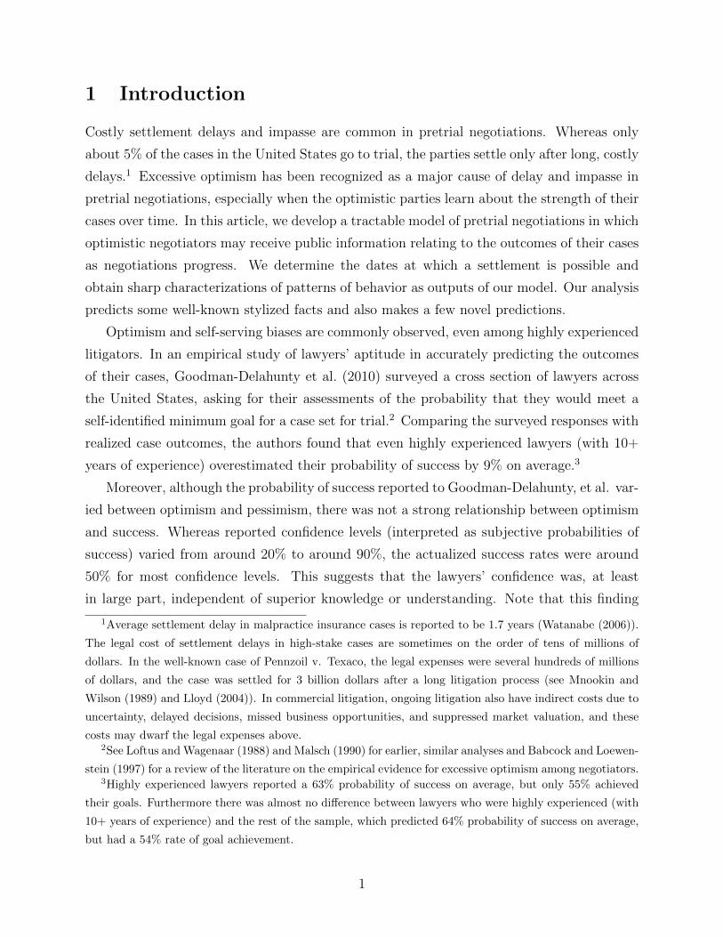
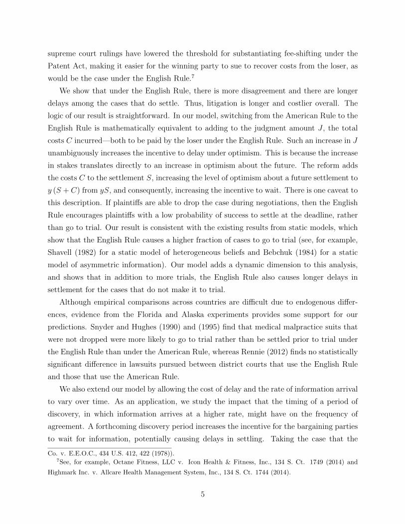
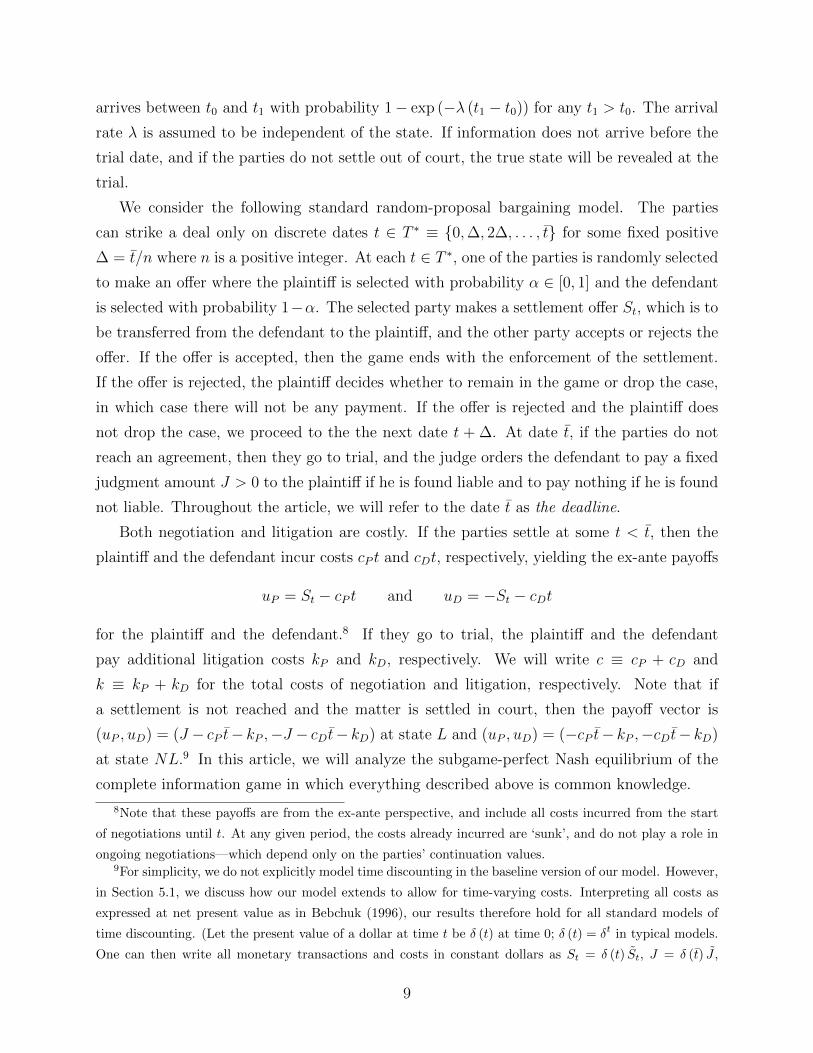
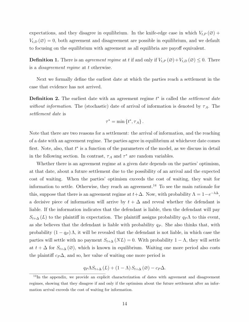
We illustrate examples of St (L) under a powerful plaintiff, balanced bargaining power,

and a powerful defendant, respectively, in Figure 1. Under a powerful plaintiff, the slope of

St (L) is negative in t (positive in −t). The farther away that the deadline is, the larger the

total of the potential costs anticipated (and consequently, the expected settlement amount),

if negotiations continue. Similarly, when the defendant is powerful, the slope of St (L) is

positive in t (negative in −t) and the farther away that the deadline is, the smaller the

expected settlement amount if negotiations ensue. When bargaining power is balanced,

St (L) does not change with time.17

16The relative bargaining power parameter α is classically interpreted as the proportion of time that each

party is able to propose a take-it-or-leave-it offer in the game theory literature. In practice, this might

be interpreted as the ease with which a proposal is made, due to economies of scale in legal paperwork,

for example. Note that we could, instead, measure bargaining power with costs, so that the plaintiff has

stronger bargaining power when her cost cP is low: cP < α1−αcD. When the parties make offers with equal

probabilities, this reduces to cP < cD. Mathematically these are equivalent and so the criterion for which

party has the stronger bargaining power and the consequent analyses would hold.17Note that the mechanism by which the balance of bargaining power impacts agreement dynamics here

is driven by the asymmetry between the plaintiff and defendant that stems from the plaintiff’s ability to

drop the case at any moment. We discuss an extension of the model in which the plaintiff must “commit”

to seeing a case through once it is initiated in section 5.2 and an online appendix.

17

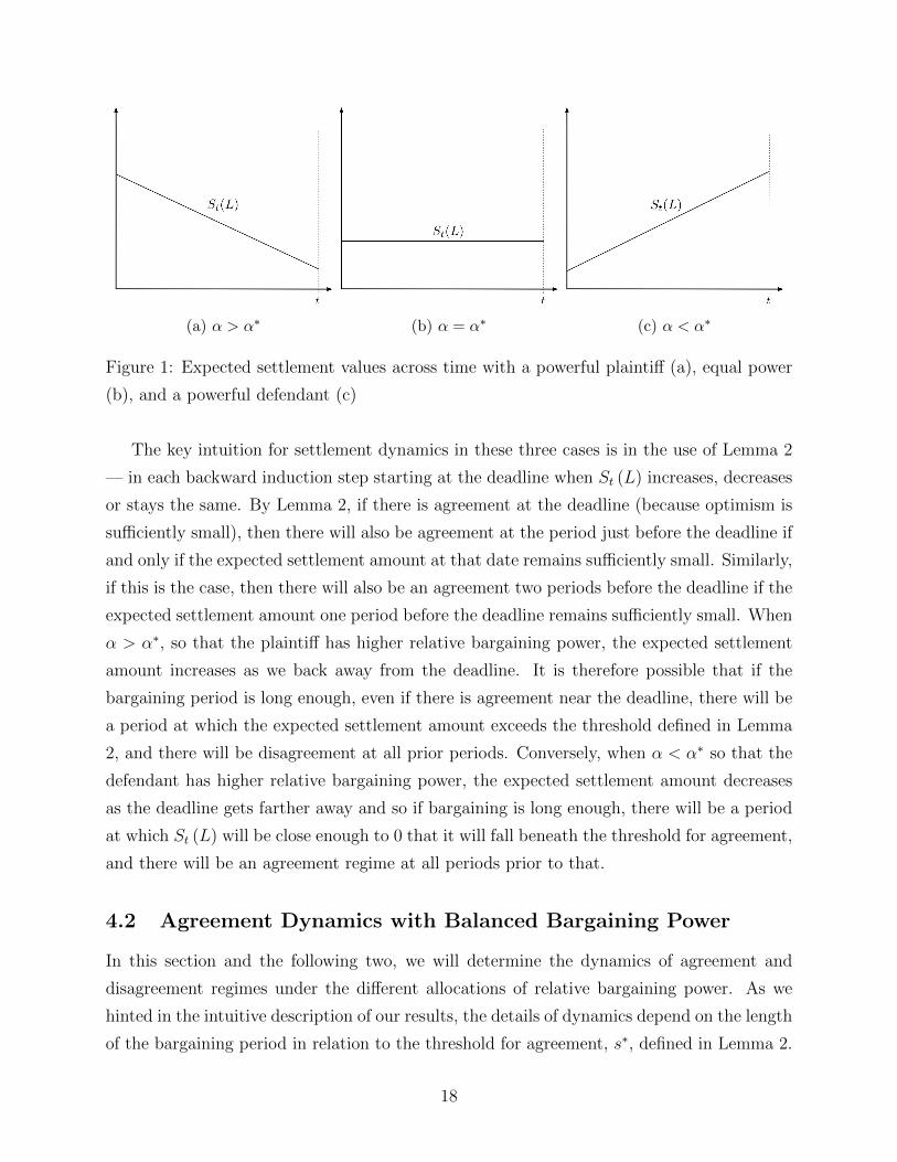
(a) α > α∗ (b) α = α∗ (c) α < α∗

Figure 1: Expected settlement values across time with a powerful plaintiff (a), equal power

(b), and a powerful defendant (c)

The key intuition for settlement dynamics in these three cases is in the use of Lemma 2

— in each backward induction step starting at the deadline when St (L) increases, decreases

or stays the same. By Lemma 2, if there is agreement at the deadline (because optimism is

sufficiently small), then there will also be agreement at the period just before the deadline if

and only if the expected settlement amount at that date remains sufficiently small. Similarly,

if this is the case, then there will also be an agreement two periods before the deadline if the

expected settlement amount one period before the deadline remains sufficiently small. When

α > α∗, so that the plaintiff has higher relative bargaining power, the expected settlement

amount increases as we back away from the deadline. It is therefore possible that if the

bargaining period is long enough, even if there is agreement near the deadline, there will be

a period at which the expected settlement amount exceeds the threshold defined in Lemma

2, and there will be disagreement at all prior periods. Conversely, when α < α∗ so that the

defendant has higher relative bargaining power, the expected settlement amount decreases

as the deadline gets farther away and so if bargaining is long enough, there will be a period

at which St (L) will be close enough to 0 that it will fall beneath the threshold for agreement,

and there will be an agreement regime at all periods prior to that.

4.2 Agreement Dynamics with Balanced Bargaining Power

In this section and the following two, we will determine the dynamics of agreement and

disagreement regimes under the different allocations of relative bargaining power. As we

hinted in the intuitive description of our results, the details of dynamics depend on the length

of the bargaining period in relation to the threshold for agreement, s∗, defined in Lemma 2.

18

As s∗ is itself a function of the level of optimism y, there is a one-to-one relationship between

how long bargaining is and how high the level of optimism needs to be for different agreement

dynamics to emerge. Throughout the remainder of this article, we will therefore frame our

results as a delineation of thresholds for the level of optimism, under a fixed maximum time

frame for negotiations, T ∗, at which bargaining lends itself to agreement and disagreement

regimes at different points in time.

When α = α∗, all time periods prior to the deadline are equivalent from the perspective

of bargaining, as St (L) does not change with t. As such, it is sufficient to check whether

the parties are willing to settle at two points: at the deadline t itself, and at the period just

before the deadline. The deadline is a special period because there cannot be any arrivals

of information that can be used for negotiation after it (or indeed, any further negotiation).

The question of agreement at the deadline, which parallels the classical static models of

pretrial bargaining with optimism, therefore depends on whether the parties’ expectations

of the outcome of a trial at court outweigh the cost of going to trial.

Specifically, the respective expected values of the plaintiff and the defendant from con-

tinuing on to trial are Vt,P (∅) = qPJ − kP and Vt,D (∅) = −qDJ − kD. There is agreement

at the deadline when there is no surplus value to continuing, i.e. Vt,P (∅) + Vt,D (∅) < 0.

Writing this conditioning in terms of optimism y = qP − qD and rearranging, we obtain a

cutoff y for agreement at the deadline. There is agreement regime at t if an only if18

y ≤ k

J≡ y.

We next derive a threshold for optimism that determines whether an agreement regime

at the deadline implies an agreement at t−∆ as well. By Lemma 2, if there is an agreement

at t, then there is an agreement regime at t−∆ if and only if St (L) ≤ s∗, where the cutoff s∗

is defined as R/y. Rearranging this condition in terms of optimism, we define the threshold

y∗ so that there is an agreement regime at t−∆ whenever there is agreement at t and

y ≤ y∗ ≡ R

St (L)=

R

J + αk − kP.

We will refer to optimism levels y > y as excessive optimism, optimism levels y ∈ [y∗, y] as

moderate optimism, and optimism levels y ≤ y∗ as low optimism.19 When y ≤ y∗ ≤ y, there

18Note, also, that there is only a settlement if the plaintiff will credibly go to trial in the absence of

settlement, as the plaintiff cannot commit not to drop the case. This is true when Vt,P (∅) ≥ 0 or qp ≥(kP + cP∆)/J .

19The cost assumption described in equation (2) ensures that y∗ ≤ y. We present the agreement dynamics

when equation (2) does not hold and y∗ > y in Proposition 8 in the online appendix.

19

is agreement both at the deadline t and in the period just before. As St (L) is invariant to

t under balanced bargaining power, this implies that St−2∆ (L) ≤ s∗ as well and so there is

an agreement regime two periods before the deadline as well. Propagating this argument

backward, there is an agreement regime at all periods, and so the parties settle right at the

start of negotiations. If y ≤ y but y > y∗, then there is agreement at the deadline, but not

at any point before then, and so the parties settle at t. If y > y and y > y∗, then the parties

do not agree at all, and the matter is decided at trial. The next result states this formally:

Proposition 1. Under balanced bargaining power (i.e. α = α∗), the parties settle immedi-

ately if optimism is low (i.e., y ≤ y∗), wait for information until the deadline t and settle at

the deadline if optimism is moderate (i.e., y∗ < y ≤ y), and wait for information until they

go to trial if optimism is excessive (i.e. y > y).

4.3 Agreement Dynamics with Powerful Plaintiff

We now assume that the plaintiff has high bargaining power, by assuming that α > α∗. In

this case, the expected settlement amount at every date t is:20

St (L) = J + α (c (t− t) + k)− (cP (t− t) + kP ) ,

which is downward sloping. The parties will continue to wait for an arrival of information

until St (L) falls below s∗ – or the deadline t – whichever comes first. Consequently, regardless

of how far off the deadline is, the parties either wait until the beginning of a window of

agreement periods prior to the deadline to settle, or they go all the way to trial, as established

in the following result.21

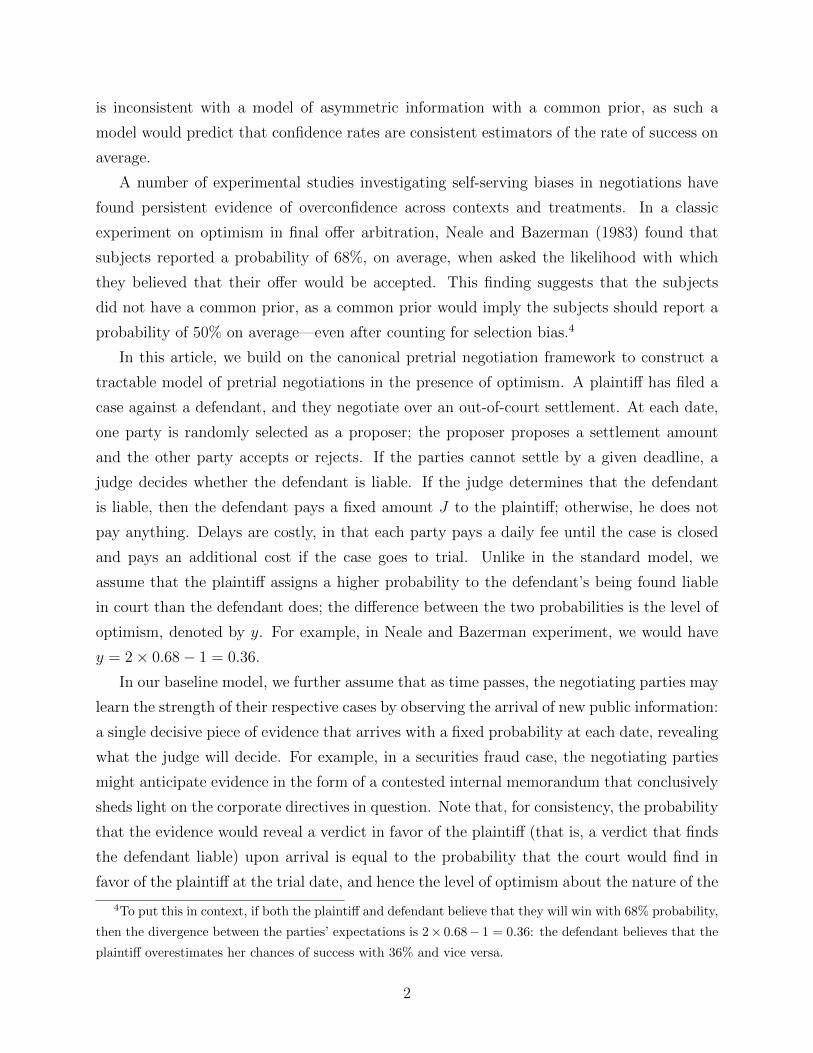
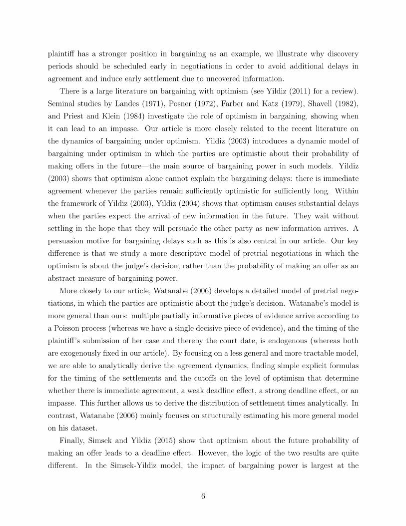
Proposition 2. Assume that the plaintiff is powerful (i.e. α > α∗). If optimism is excessive,

the parties wait for information without settling until they go to trial; otherwise, they wait

for information until some date t∗ and settle there. More specifically, if y > y, there is

a disagreement regime at every t ∈ T ∗; otherwise, there is a disagreement regime at every

t < t∗ and an agreement regime at every t ≥ t∗ where

t∗ = max {t ∈ T ∗|St (L) > s∗} .

In particular, under moderate optimism (i.e. y∗ ≤ y ≤ y), as long as they do not receive an

information, the parties wait until the deadline t and settle there in equilibrium.

20This follows from Lemma 1 and inequality (3).21In the proposition we use the convention that max of empty set is −∞.

20

Proof. First, consider the case that y > y ≥ y∗. As y > y∗, it follows that St (L) > s∗.

Moreover, as α > α∗, St (L) is decreasing in t. Hence, St (L) > s∗ for every t ≤ t. Therefore,

by Lemma 2, there is a disagreement regime at each t < t. Moreover, as y > y, there is

also a disagreement regime at t. Now consider the case y ≤ y, so that there is an agreement

regime at t. By inductive application of the second part of Lemma 2, there is an agreement

regime at each t ≥ t∗ because St+∆ (L) ≤ s∗. Moreover, by the first part of Lemma 2, there

is a disagreement regime at each t < t∗ because St+∆ (L) > s∗.

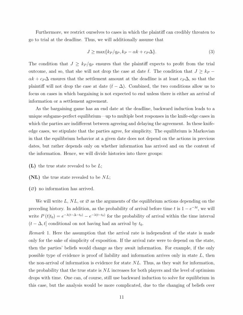
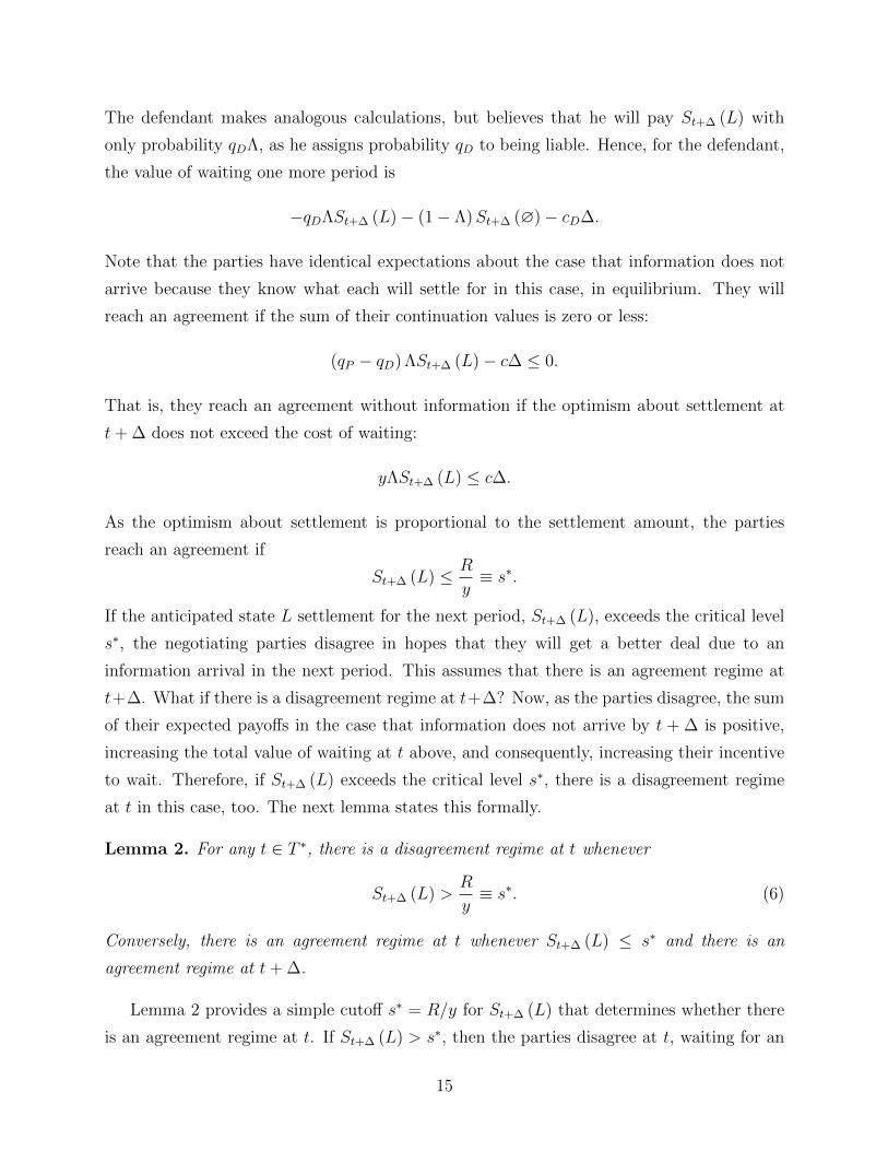
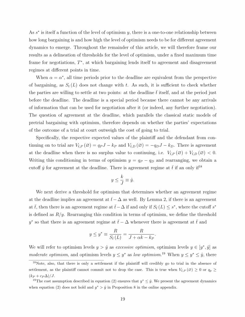
(a) α > α∗ and y ≤ y∗ (b) α > α∗ and y∗ ≤ y ≤ y (c) α > α∗ and y > y

Figure 2: Agreement dynamics under a strong plaintiff

As we have discussed before, the parties settle when there is an arrival, which eliminates

any difference of opinion. For contingencies without an arrival, Proposition 2 presents an

intuitive pattern of behavior, depending on the level of optimism, as summarized in Figure

2. When the parties are excessively optimistic, i.e., when y > y, the negotiations result in

an impasse, and a judge determines whether or not the defendant is liable after a costly

litigation process. This case is illustrated in panel (c) of Figure 2. Even at t = t, St (L) > s∗

and there is no agreement at the deadline. As we consider earlier dates, St (L) increases,

and so we cannot have an agreement regime at any of these dates either. When the parties

are moderately optimistic, i.e., when y∗ ≤ y ≤ y, a strong form of the deadline effect is

exhibited in equilibrium: the parties wait for information until the deadline, t, and reach an

agreement at the steps of the courthouse if information does not arrive by then. This case is

illustrated in panel (b) of Figure 2. As y < y, there is an agreement regime at the deadline.

However, St (L) > s∗ and so there is a disagreement regime at t = t−∆, and as we consider

earlier dates, St (L) increases, so that there is no other date with an agreement regime.

Finally, when the optimism level is low, i.e., when y < y∗, a weak form of the deadline effect

is exhibited in equilibrium: the parties wait for information until a date t∗ that begins a

21

window of agreement periods prior to the deadline, and settle at t∗ if information does not

arrive by then. They would have agreed at any date in the window between t∗ and the

deadline, as well. This case is illustrated in panel (a) of Figure 2. As y < y, there is again

an agreement regime at the deadline. As y < y∗, St (L) ≤ s∗, and so as we consider earlier

dates, there is also an agreement regime at every date until t∗. As St (L) is increasing as we

consider earlier dates, St (L) > s∗ for every date t before t∗, and so there is no agreement

regime at any such date. It is crucial to observe that neither the cutoffs y∗ and y nor the

length t − t∗ of the interval of agreement regimes is a function of t. No matter how far the

deadline is, the parties wait for a fixed neighborhood of the deadline to reach an agreement.

4.4 Agreement Dynamics with Powerful Defendant

We now assume that the defendant has a stronger position in bargaining by assuming that

α < α∗. We then determine whether there is an agreement or a disagreement regime at

any given t. In particular, we establish that there is either an immediate agreement, or the

strong form of the deadline effect (in which the parties wait until the deadline to settle) or

an impasse.

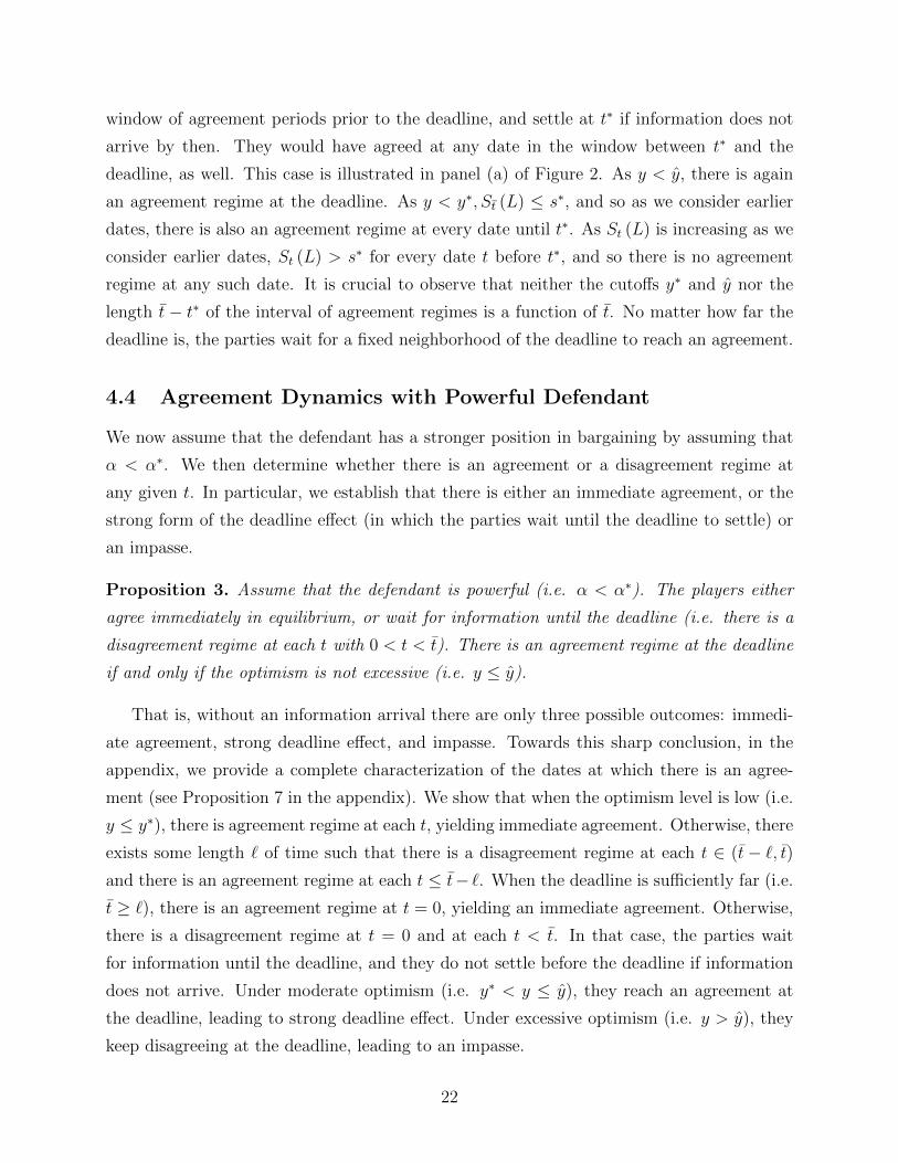
Proposition 3. Assume that the defendant is powerful (i.e. α < α∗). The players either

agree immediately in equilibrium, or wait for information until the deadline (i.e. there is a

disagreement regime at each t with 0 < t < t). There is an agreement regime at the deadline

if and only if the optimism is not excessive (i.e. y ≤ y).

That is, without an information arrival there are only three possible outcomes: immedi-

ate agreement, strong deadline effect, and impasse. Towards this sharp conclusion, in the

appendix, we provide a complete characterization of the dates at which there is an agree-

ment (see Proposition 7 in the appendix). We show that when the optimism level is low (i.e.

y ≤ y∗), there is agreement regime at each t, yielding immediate agreement. Otherwise, there

exists some length ` of time such that there is a disagreement regime at each t ∈ (t− `, t)and there is an agreement regime at each t ≤ t− `. When the deadline is sufficiently far (i.e.

t ≥ `), there is an agreement regime at t = 0, yielding an immediate agreement. Otherwise,

there is a disagreement regime at t = 0 and at each t < t. In that case, the parties wait

for information until the deadline, and they do not settle before the deadline if information

does not arrive. Under moderate optimism (i.e. y∗ < y ≤ y), they reach an agreement at

the deadline, leading to strong deadline effect. Under excessive optimism (i.e. y > y), they

keep disagreeing at the deadline, leading to an impasse.

22

Under a powerful plaintiff, because of a decreasing settlement St (L), the partial charac-

terization in Lemma 2 was sufficient to pin down the agreement dynamics. Whether there

was an agreement regime at t depended on whether the settlement St+∆ (L) in the next

period was above the cutoff s∗. Under a powerful defendant, the settlement St (L) and thus

the incentive to wait are increasing over time, and hence there can be an agreement at t

while there is a disagreement at t + ∆. The task of determining whether that occurs at a

given period is more complex, and the result depends on the conditional expectation of St (L)

over upcoming dates of disagreement, rather than St+∆ (L).

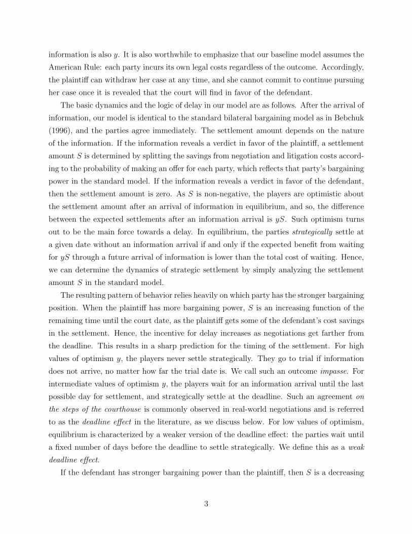
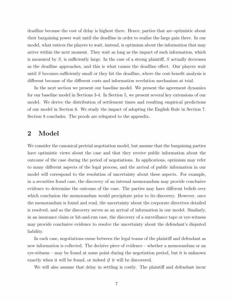
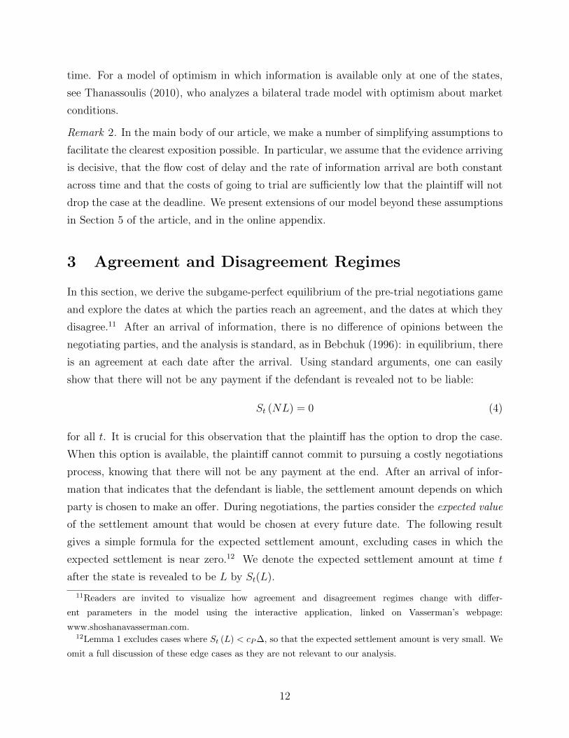
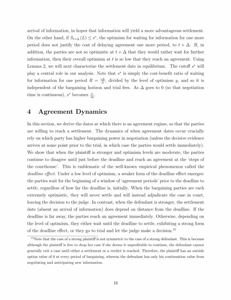
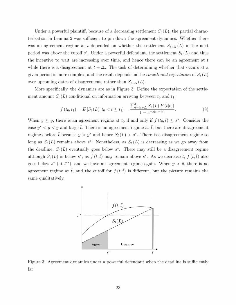
More specifically, the dynamics are as in Figure 3. Define the expectation of the settle-

ment amount St (L) conditional on information arriving between t0 and t1:

f (t0, t1) = E [St (L) |t0 < t ≤ t1] =

∑t1t=t0+∆ St (L)P (t|t0)

1− e−λ(t1−t0). (8)

When y ≤ y, there is an agreement regime at t0 if and only if f (t0, t) ≤ s∗. Consider the

case y∗ < y < y and large t. There is an agreement regime at t, but there are disagreement

regimes before t because y > y∗ and hence St (L) > s∗. There is a disagreement regime so

long as St (L) remains above s∗. Nonetheless, as St (L) is decreasing as we go away from

the deadline, St (L) eventually goes below s∗. There may still be a disagreement regime

although St (L) is below s∗, as f (t, t) may remain above s∗. As we decrease t, f (t, t) also

goes below s∗ (at t∗∗), and we have an agreement regime again. When y > y, there is no

agreement regime at t, and the cutoff for f (t, t) is different, but the picture remains the

same qualitatively.

Figure 3: Agreement dynamics under a powerful defendant when the deadline is sufficiently

far

23

4.5 Agreement Dynamics in Continuous Time–A Discussion

In the main body of our article, we considered a model in which bargaining occurs across

discrete time periods. Our results become even simpler in the continuous-time limit ∆→ 0.

In this section we discuss the equilibrium behavior in greater detail for the continuous-time

limit. We focus on the case that α > α∗ for ease of exposition. The case that α < α∗ follows

similarly and is fully worked out in the online appendix.

In the continuous-time limit, the relevant values in equilibrium (namely y, y∗, s∗, and

(t− t∗)) take very simple intuitive form. The cutoff y for impasse is already simple:

y ≡ k/J,

i.e., the ratio of the trial cost k to the judgment amount J . As in static models, when the

optimism level exceeds this ratio, bargaining results in an impasse, and the parties settle

otherwise. The cutoff y∗ for the strong and the weak forms of the deadline effect becomes

y∗ ≡ c

λ· 1

J + αk − kP.

Here, c/λ is the cost-benefit ratio of waiting for information, and J+αk−kP is the settlement

at the deadline if information arrives at the deadline and shows that the defendant is liable.

As stated in Proposition 2, if the evidence does not arrive, then in equilibrium, for

moderate values y ∈ [y∗, y] of optimism, the parties exhibit a strong form of the deadline

effect by waiting exactly until the deadline to settle. For lower values y < y∗ of optimism,

the parties exhibit a weak form of the deadline effect by waiting for a window of agreement

periods prior to the deadline to settle. For extreme values y > y of optimism, the negotiations

result in impasse.

We will next illustrate the agreement dynamics and derive an explicit simple formula for

the strategic settlement date t∗.22 As shown in Figure 2, t∗ is determined by the intersection

of St (L) with s∗, which simply becomes

s∗ ≡ c

λ· 1

y, (9)

the cost-benefit ratio c/λ, divided by the level y of optimism, in the continuous-time limit.

By Lemma 2, an agreement regime at t carries over to a previous date if and only if St (L) is

lower than this ratio. Moreover, under low optimism, the settlement date without an arrival

of information is simply given by

St∗ (L) = s∗,

22Recall that the realized settlement date is the minimum of t∗ and the date of information arrival, which

is stochastic.

24

provided that S0 (L) ≥ s∗. By substituting (5) and (9) in the above equality, we obtain

t∗ = t−cλy− (J + αk − kP )

(α− α∗) c, (10)

which can also be written as

t∗ = t− (y∗ − y) /y

(α− α∗) cSt (L) . (11)

Note that the difference between the strategic settlement date t∗ and the deadline t is in-

dependent of the deadline. No matter how far off the deadline is, the parties wait for

information until they reach a fixed neighborhood of the deadline and settle there regardless

of the arrival of information.

How close will they come to the deadline? This depends on several factors. First, the

more optimistic the negotiating parties are, the closer they get to the deadline: t − t∗ is

proportional to (y∗ − y) /y. As the level of optimism approaches to the cutoff, the length

t− t∗ shrinks to zero, and the parties exhibit nearly strong form of deadline effect. On the

other hand, for arbitrary small values of optimism, they can settle arbitrarily far away from

the deadline: t− t∗ →∞ as y → 0. In particular, they reach an immediate agreement when

y < ymin ≡c/λ

(α− a∗) ct+ (J + αk − kP ).

Here, ymin is the smallest level of optimism under which there is delay in equilibrium. Inter-

estingly, ymin is decreasing in t and approaches zero as t→∞. That is, no matter how small

the optimism is, there will be some amount of delay due to the weak form of deadline effect

when the deadline is sufficiently far. A similar delay occurs when the cost-benefit ratio c/λ

is small. The other two factors that determine the length t − t∗ of agreement regimes are

St (L) = J + αk− kP and the strength α− α∗ of the bargaining position of the plaintiff. By

(10), t− t∗ is decreasing in St (L) and shrinks to zero as St (L) approach the ratio cλy≡ s∗.

Similarly, t−t∗ is decreasing in α−α∗. In summary, the deadline effect gets stronger with the

level of optimism y, the bargaining power of the plaintiff (α− α∗) and St (L) = J +αk−kP .

5 Extensions

In our main model, we made several restrictive assumptions for the sake of exposition. We

assumed that the arrival rate is fixed over time, that the plaintiff can drop her lawsuit

and that evidence, should it arrive, is decisive. Despite the seeming restrictiveness of these

25

simplifying assumptions, the main intuitions of our results hold even when these assumptions

are relaxed. In this section, we present an extension of our model in which litigation costs

and arrival rates can vary with time. This extension is of particular interest as negotiations

often span intermittent periods of high and low activity. For example, there will be higher

activity in periods of discovery and jury selection. These periods are anticipated, and, as may

be expected, they affect the timing of agreement/disagreement regimes. For this reason, we

detail how our model can account for this case below. In addition, we briefly discuss further

extensions of our model to cover the other major assumptions made toward our baseline

results. We defer the details of these further extensions to the online appendix.

5.1 Time-Varying Arrival Rates

In our baseline model, we assume that the cost of litigation and the arrival rate of evidence

are static throughout the bargaining process. In reality, the rate of evidence might vary

across time. For example, the probability of evidence might be higher during periods of

discovery or jury selection. The litigation costs could also be higher in these periods. In this

section, we show that our framework for determining periods of agreement and disagreement

can be naturally extended to cover this case. In particular, we extend our baseline model

to allow the costs and the rate of arrival to be arbitrarily time varying, according to any

well-behaved functions c(t) and λ(t).

For any time varying arrival rate that can be described as an integrable function λ(t),

write Λ(t) = 1− e−∫ t+∆t λ(t′)dt′ for the probability of an arrival at period t. Similarly, let the

litigation costs cP and cD be functions of time, so that the cost of waiting one more period

at t is cP (t)∆ and cD(t)∆ for the plaintiff and the defendant, respectively. We write c(t)∆

for the total cost of delay at time t, where c (t) = cP (t) + cD (t). We therefore write the cost

benefit ratio in this case as a function of t, R(t) = c(t)∆Λ(t)

. We extend Lemma 2 as follows:

Lemma 3. For any t ∈ T ∗, there is a disagreement regime at t whenever

St+∆ (L) >1

y

c (t) ∆

Λ(t)≡ s∗(t). (12)

Conversely, there is an agreement regime at t whenever St+∆ (L) ≤ s∗(t) and there is an

agreement regime at t+ ∆.

Lemma 3 extends the characterization for agreement by making the cutoff for agreement

time-dependent. The only change is that c (t) and Λ(t) are now time-dependent, rather

than fixed parameters, whereas all the other parameters such as St(L) and y, which are

26

independent of λ(t), remain as in the static case. Note that as in the static case, the cutoff

s∗(t) becomes

s∗(t) =c(t)

λ(t)y

in the continuous-time limit. That is, the same formula applies, except that the particular

value of the cost-benefit ratio c/λ depends on the time t at which it is being considered.

Note also that the cutoff s∗(t) is proportional to the cost-benefit ratio c (t) /λ(t).

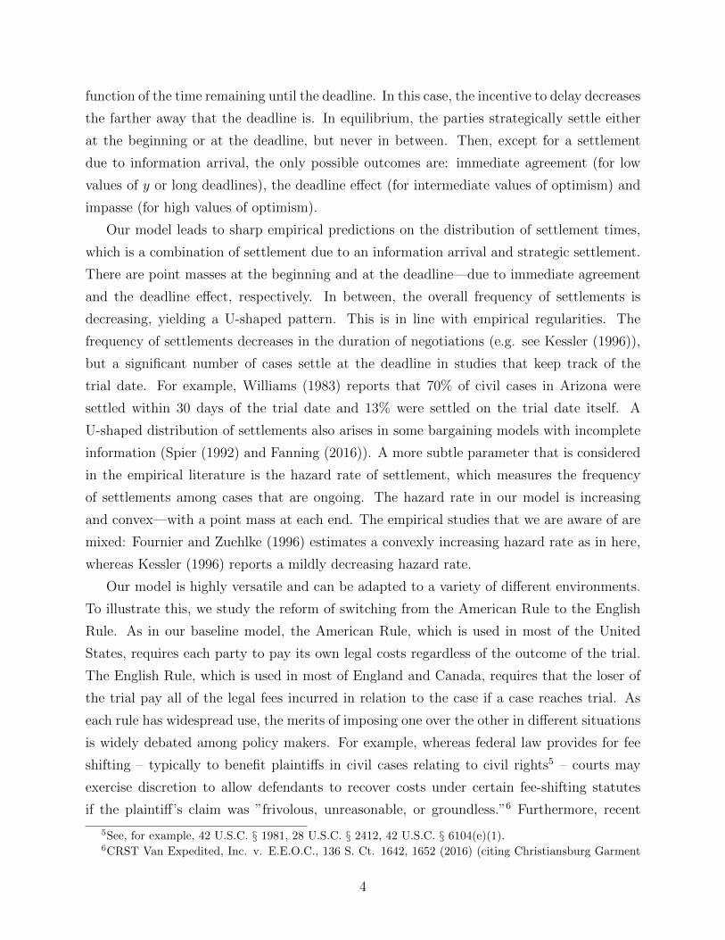
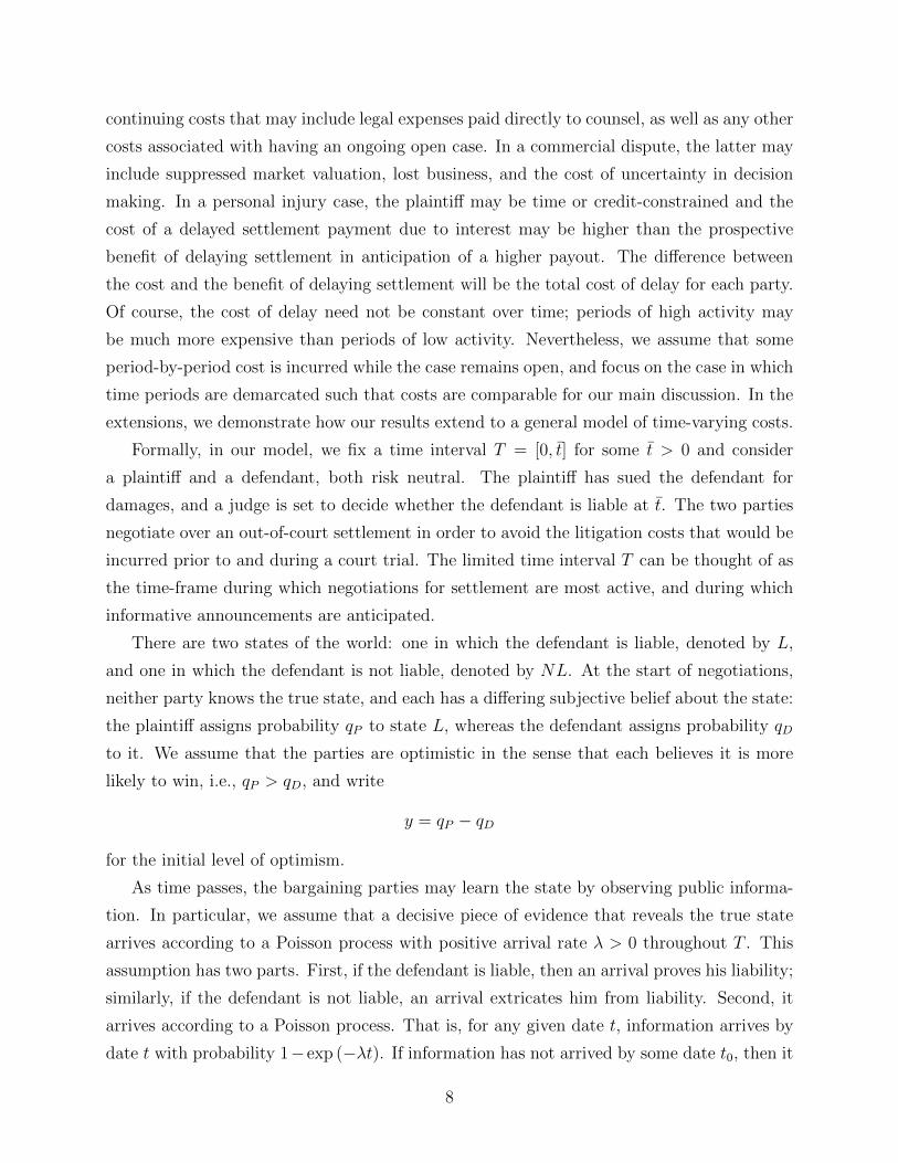
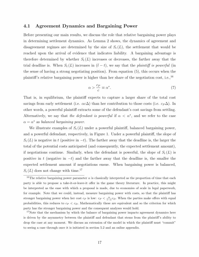
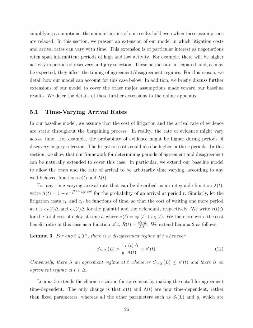
Figure 4: Agreement dynamics under a powerful plaintiff with a time-varying rate of arrival

As in previous sections, one can use Lemma 3 to determine the agreement dynamics

in specific situations by comparing the expected settlement amount St (L) to s∗(t). As an

illustrative example, consider the case of a powerful plaintiff as in Section 4.3 and suppose

that y < y so that there is agreement at the deadline. Suppose, further, that c (t) /λ(t) is

some function such that s∗(t) is given by the dashed curve in Figure 4. As there is agreement

at the deadline, and s∗(t) is greater than St(L), there is also agreement at the interval of

periods t3 < t < t where t3 is the first period before the deadline at which s∗(t) = St(L). By

Lemma 3, there is disagreement during the periods between dates 0 and t1, and between t2

and t3. However, our lemma is silent on the periods between dates t1 and t2.

To determine whether there is agreement at a given date t0, we would need to compare

s∗(t0) against E[St(L)|t0 ≤ t ≤ t3] where the expectation of St(L) is calculated analogously

to the static case, as given in equation (8). That is, there is an agreement at t0 if f(t0, t3) <

s∗(t0) where

f(t0, t3) = E[St(L)|t0 ≤ t ≤ t3] =

∑t3t=t0+∆ St(L)P (t|t0)

1− e−∫ t3t0λ(t)dt

,

27

and the probability P (t|t0) = e−

∫ t−∆t0

λ(t)dtΛ(t − ∆) is computed using the time varying

function λ(t).

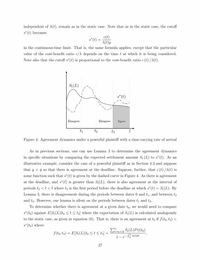
Figure 5: Plot of cost-benefit ratio c(t)/λ(t) given by a baseline cost to arrival rate ratio

c∗B/λ∗B and a discovery ratio c∗D/λ

∗D, under different schedules for the discovery period TD

This might have direct implications for scheduling periods of discovery, during which λ(t)

is particularly high—and during which, legal teams are more active so that the per-period

litigation fees may be higher as well. As a simple case, imagine that λ(t)/c(t) can take two

values: a baseline rate λB/cB and a discovery rate λD/cD where λD � λB, and that discovery

takes place over some fixed interval of periods TD. Our model shows that the choice of when

TD will take place can influence the settlement dynamics.

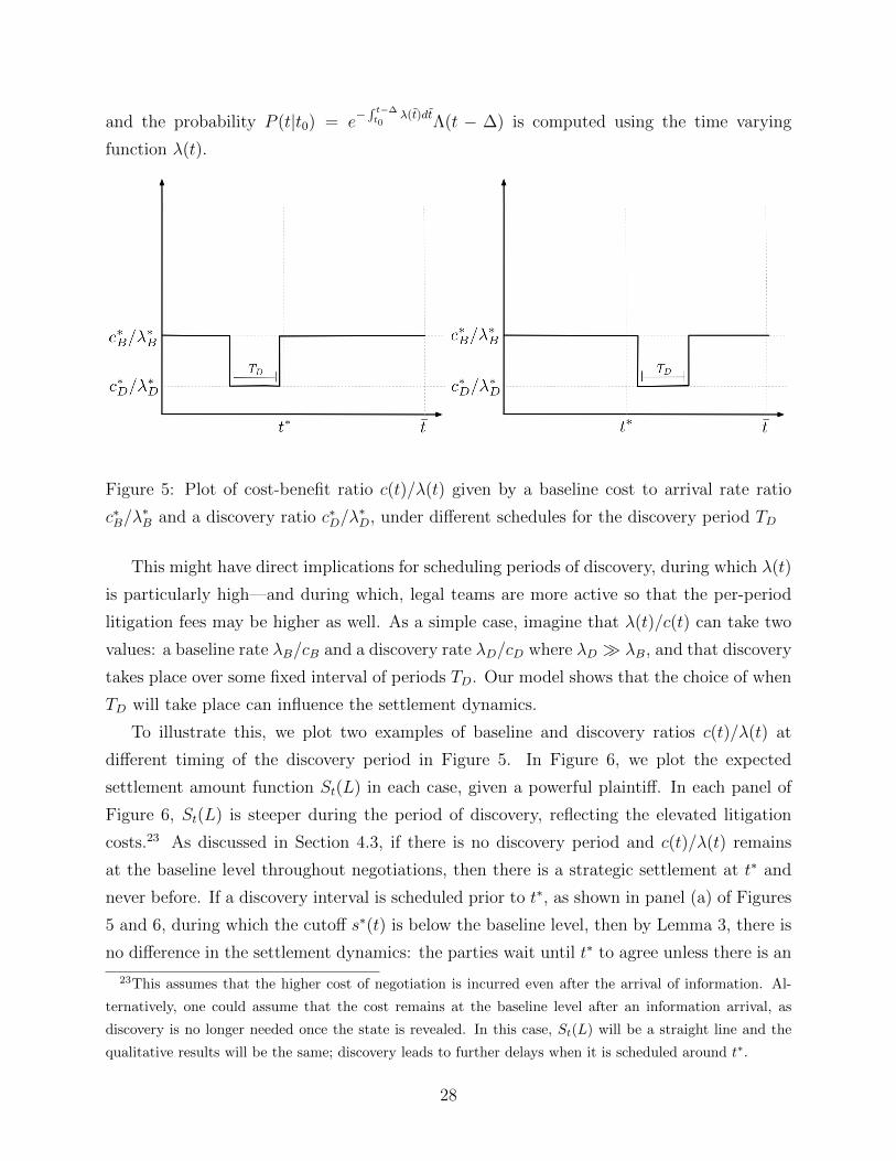
To illustrate this, we plot two examples of baseline and discovery ratios c(t)/λ(t) at

different timing of the discovery period in Figure 5. In Figure 6, we plot the expected

settlement amount function St(L) in each case, given a powerful plaintiff. In each panel of

Figure 6, St(L) is steeper during the period of discovery, reflecting the elevated litigation

costs.23 As discussed in Section 4.3, if there is no discovery period and c(t)/λ(t) remains

at the baseline level throughout negotiations, then there is a strategic settlement at t∗ and

never before. If a discovery interval is scheduled prior to t∗, as shown in panel (a) of Figures

5 and 6, during which the cutoff s∗(t) is below the baseline level, then by Lemma 3, there is

no difference in the settlement dynamics: the parties wait until t∗ to agree unless there is an

23This assumes that the higher cost of negotiation is incurred even after the arrival of information. Al-

ternatively, one could assume that the cost remains at the baseline level after an information arrival, as

discovery is no longer needed once the state is revealed. In this case, St(L) will be a straight line and the

qualitative results will be the same; discovery leads to further delays when it is scheduled around t∗.

28

Figure 6: Agreement dynamics in an extension of the left-most panel of Figure 2, in which a

discovery period TD with higher cost to arrival rate ratio c∗D/λ∗D is scheduled as in Figure 5

arrival of information. However, as the rate of arrival is higher during TD, the probability of

an arrival of information – and therefore, of agreement due to information arriving – is higher

during this period. Thus, scheduling TD to be as early as possible increases the aggregate

probability of early settlement.

In contrast, if TD begins after t∗, as in panel (b) of Figures 5 and 6, then there is

disagreement prior to t∗ as before, but now there is disagreement during TD as well. Moreover,

the higher rate of arrival during discovery will entice the parties to wait for TD, creating

further incentive for disagreement prior to TD. Depending on when TD is placed, this may

postpone the first strategic settlement date to the end of the discovery period all together.

5.2 Commitment

In our main model, we have assumed that the plaintiff can drop her lawsuit at any point

in the negotiations up to the trial date. This assumption, which we made in the spirit of

modeling reality more closely, provides an inherent asymmetry in the bargaining power of

the plaintiff and the defendant. In particular, it implies that St(NL) = 0. That is, upon

discovery that the defendant is not liable, neither the plaintiff nor the defendant are liable

for any further costs. In the online appendix, we explore the consequences of a rule by

which once a plaintiff has initiated a lawsuit, she must commit to the case and cannot leave

it without either a settlement or a court decision. With this alternative assumption, the

balance of bargaining power between the plaintiff and the defendant does not play a role in

29

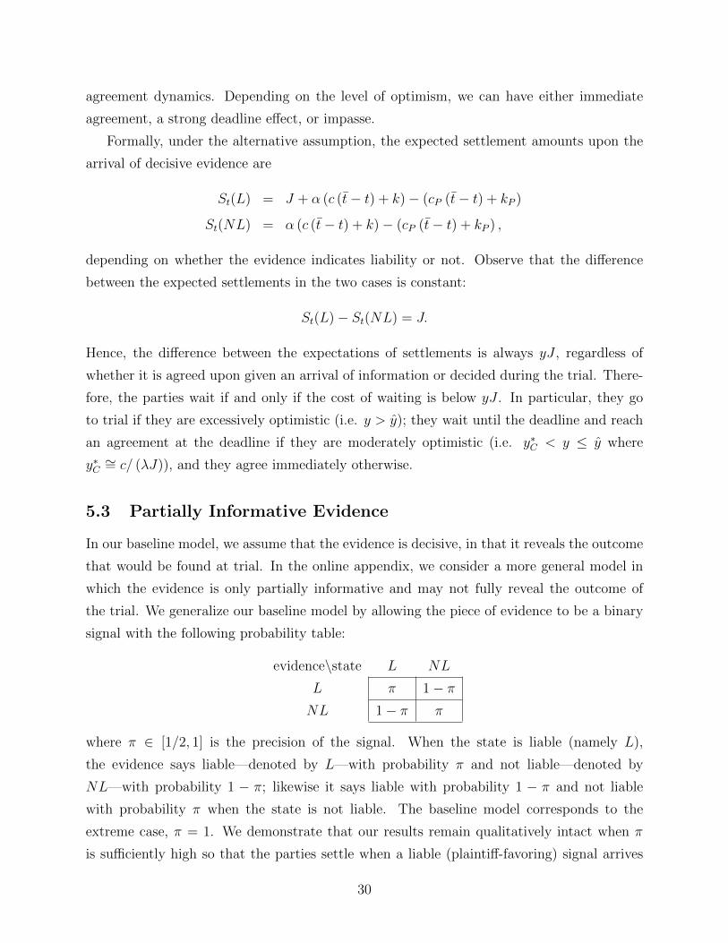
agreement dynamics. Depending on the level of optimism, we can have either immediate

agreement, a strong deadline effect, or impasse.

Formally, under the alternative assumption, the expected settlement amounts upon the

arrival of decisive evidence are

St(L) = J + α (c (t− t) + k)− (cP (t− t) + kP )

St(NL) = α (c (t− t) + k)− (cP (t− t) + kP ) ,

depending on whether the evidence indicates liability or not. Observe that the difference

between the expected settlements in the two cases is constant:

St(L)− St(NL) = J.

Hence, the difference between the expectations of settlements is always yJ , regardless of

whether it is agreed upon given an arrival of information or decided during the trial. There-

fore, the parties wait if and only if the cost of waiting is below yJ . In particular, they go

to trial if they are excessively optimistic (i.e. y > y); they wait until the deadline and reach

an agreement at the deadline if they are moderately optimistic (i.e. y∗C < y ≤ y where

y∗C∼= c/ (λJ)), and they agree immediately otherwise.

5.3 Partially Informative Evidence

In our baseline model, we assume that the evidence is decisive, in that it reveals the outcome

that would be found at trial. In the online appendix, we consider a more general model in

which the evidence is only partially informative and may not fully reveal the outcome of

the trial. We generalize our baseline model by allowing the piece of evidence to be a binary

signal with the following probability table:

evidence\state L NL

L π 1− πNL 1− π π

where π ∈ [1/2, 1] is the precision of the signal. When the state is liable (namely L),

the evidence says liable—denoted by L—with probability π and not liable—denoted by

NL—with probability 1 − π; likewise it says liable with probability 1 − π and not liable

with probability π when the state is not liable. The baseline model corresponds to the

extreme case, π = 1. We demonstrate that our results remain qualitatively intact when π

is sufficiently high so that the parties settle when a liable (plaintiff-favoring) signal arrives

30

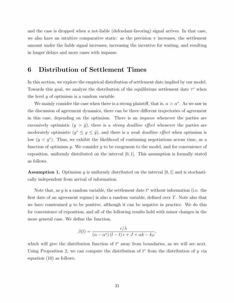
and the case is dropped when a not-liable (defendant-favoring) signal arrives. In that case,

we also have an intuitive comparative static: as the precision π increases, the settlement

amount under the liable signal increases, increasing the incentive for waiting, and resulting

in longer delays and more cases with impasse.

6 Distribution of Settlement Times

In this section, we explore the empirical distribution of settlement date implied by our model.

Towards this goal, we analyze the distribution of the equilibrium settlement date τ ∗ when

the level y of optimism is a random variable.

We mainly consider the case when there is a strong plaintiff, that is, α > α∗. As we saw in

the discussion of agreement dynamics, there can be three different trajectories of agreement

in this case, depending on the optimism. There is an impasse whenever the parties are

excessively optimistic (y > y), there is a strong deadline effect whenever the parties are

moderately optimistic (y∗ ≤ y ≤ y), and there is a weak deadline effect when optimism is

low (y < y∗). Thus, we exhibit the likelihood of continuing negotiations across time, as a

function of optimism y. We consider y to be exogenous to the model, and for convenience of

exposition, uniformly distributed on the interval [0, 1]. This assumption is formally stated

as follows.

Assumption 1. Optimism y is uniformly distributed on the interval [0, 1] and is stochasti-

cally independent from arrival of information.

Note that, as y is a random variable, the settlement date t∗ without information (i.e. the

first date of an agreement regime) is also a random variable, defined over T . Note also that

we have constrained y to be positive, although it can be negative in practice. We do this

for convenience of exposition, and all of the following results hold with minor changes in the

more general case. We define the function,

β(t) =c/λ

(α− α∗) (t− t) c+ J + αk − kP,

which will give the distribution function of t∗ away from boundaries, as we will see next.

Using Proposition 2, we can compute the distribution of t∗ from the distribution of y via

equation (10) as follows.

31

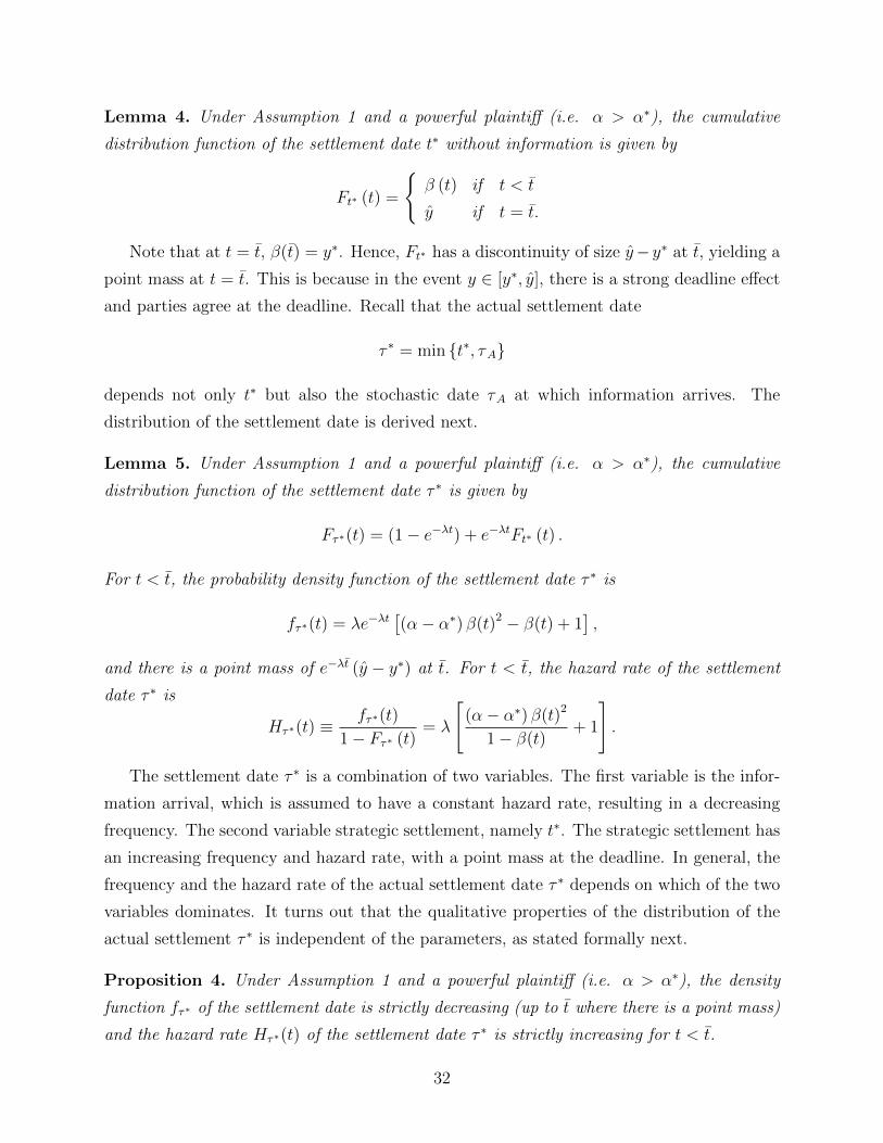
Lemma 4. Under Assumption 1 and a powerful plaintiff (i.e. α > α∗), the cumulative

distribution function of the settlement date t∗ without information is given by

Ft∗ (t) =

{β (t) if t < t

y if t = t.

Note that at t = t, β(t) = y∗. Hence, Ft∗ has a discontinuity of size y− y∗ at t, yielding a

point mass at t = t. This is because in the event y ∈ [y∗, y], there is a strong deadline effect

and parties agree at the deadline. Recall that the actual settlement date

τ ∗ = min {t∗, τA}

depends not only t∗ but also the stochastic date τA at which information arrives. The

distribution of the settlement date is derived next.

Lemma 5. Under Assumption 1 and a powerful plaintiff (i.e. α > α∗), the cumulative

distribution function of the settlement date τ ∗ is given by

Fτ∗(t) = (1− e−λt) + e−λtFt∗ (t) .

For t < t, the probability density function of the settlement date τ ∗ is

fτ∗(t) = λe−λt[(α− α∗) β(t)2 − β(t) + 1

],

and there is a point mass of e−λt (y − y∗) at t. For t < t, the hazard rate of the settlement

date τ ∗ is

Hτ∗(t) ≡fτ∗(t)

1− Fτ∗ (t)= λ

[(α− α∗) β(t)2

1− β(t)+ 1

].

The settlement date τ ∗ is a combination of two variables. The first variable is the infor-

mation arrival, which is assumed to have a constant hazard rate, resulting in a decreasing

frequency. The second variable strategic settlement, namely t∗. The strategic settlement has

an increasing frequency and hazard rate, with a point mass at the deadline. In general, the

frequency and the hazard rate of the actual settlement date τ ∗ depends on which of the two

variables dominates. It turns out that the qualitative properties of the distribution of the

actual settlement τ ∗ is independent of the parameters, as stated formally next.

Proposition 4. Under Assumption 1 and a powerful plaintiff (i.e. α > α∗), the density

function fτ∗ of the settlement date is strictly decreasing (up to t where there is a point mass)

and the hazard rate Hτ∗(t) of the settlement date τ ∗ is strictly increasing for t < t.

32

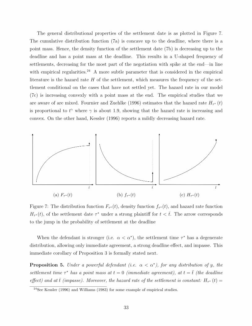
The general distributional properties of the settlement date is as plotted in Figure 7.

The cumulative distribution function (7a) is concave up to the deadline, where there is a

point mass. Hence, the density function of the settlement date (7b) is decreasing up to the

deadline and has a point mass at the deadline. This results in a U-shaped frequency of

settlements, decreasing for the most part of the negotiation with spike at the end—in line

with empirical regularities.24 A more subtle parameter that is considered in the empirical

literature is the hazard rate H of the settlement, which measures the frequency of the set-

tlement conditional on the cases that have not settled yet. The hazard rate in our model

(7c) is increasing convexly with a point mass at the end. The empirical studies that we

are aware of are mixed. Fournier and Zuehlke (1996) estimates that the hazard rate Hτ∗ (t)

is proportional to tγ where γ is about 1.9, showing that the hazard rate is increasing and

convex. On the other hand, Kessler (1996) reports a mildly decreasing hazard rate.

(a) Fτ∗(t) (b) fτ∗(t) (c) Hτ∗(t)

Figure 7: The distribution function Fτ∗(t), density function fτ∗(t), and hazard rate function

Hτ∗(t), of the settlement date τ ∗ under a strong plaintiff for t < t. The arrow corresponds

to the jump in the probability of settlement at the deadline

When the defendant is stronger (i.e. α < α∗), the settlement time τ ∗ has a degenerate

distribution, allowing only immediate agreement, a strong deadline effect, and impasse. This

immediate corollary of Proposition 3 is formally stated next.

Proposition 5. Under a powerful defendant (i.e. α < α∗), for any distribution of y, the

settlement time τ ∗ has a point mass at t = 0 (immediate agreement), at t = t (the deadline

effect) and at t (impasse). Moreover, the hazard rate of the settlement is constant: Hτ∗ (t) =

24See Kessler (1996) and Williams (1983) for some example of empirical studies.

33

λ for all t ∈ (0, t). The probability of immediate agreement is increasing in t and decreasing

in α.

The qualitative properties of the settlement distribution under a powerful defendant

mirror the case of a powerful plaintiff with the following exceptions. First, although the

frequency of settlement has still a U shape, there is now a point mass at the beginning.25

That is, a significant portion of cases settle immediately, and the portion of such cases

gets larger when the deadline is pushed away (perhaps because of the backlog of cases in

the court) or when the defendant gets a stronger bargaining position (e.g. if the cost cD

of negotiation for the defendant decreases or the cost for the plaintiff increases). Second,

the hazard rate in the interior is constant, rather than convexly increasing. This is simply

because any such settlement must be due to an information arrival, which is assumed to

have a constant hazard rate.

If the data-set includes both cases with powerful defendants and with powerful plaintiffs,

then the settlement date τ ∗ still has a point mass at the beginning (t = 0), at the deadline

(t = t) and at the impasse (t = t). For t ∈ (0, t), the hazard rate is convexly increasing and

the frequency fτ∗ of the settlements is decreasing. We formally state this below.

Proposition 6. Under Assumption 1, when α is randomly chosen from the full support

[0, 1], the density function fτ∗ of the settlement date is strictly decreasing from t = 0 up to

t, and has point masses at t = 0, t = t and t = t. The hazard rate Hτ∗(t) of the settlement

date τ ∗ is strictly increasing for t < t.

When there is a possibility of having either a powerful plaintiff or a powerful defendant,

the density of settlements is a weighted combination of the settlement densities in each case.

The density, and therefore the frequency, of settlement is decreasing for t ∈ (0, t), as it is

driven by the density of settlements with powerful plaintiffs with zero density among settle-

ments with powerful defendants. At the points t = 0, t = t and t = t, there are point masses

stemming from both cases, so that the point masses generated by the settlement densities

in cases of powerful defendants are amplified by those from the densities of powerful plain-

tiffs. The resulting average density is qualitatively identical to that of a powerful plaintiff.

Thus, the prediction of a U-shaped frequency of settlements is robust to assumptions about

a particular party being more powerful. Similarly, the aggregate hazard rate is convexly

increasing as in the case of a powerful plaintiff, so that the prediction of a convex hazard

rate is also robust to assumptions about the relative bargaining power distribution.

25Such a point mass occurs even under a powerful plaintiff when the probability Pr(y < 0) of pessimism

is positive.

34

All in all, the empirical implications of our model are similar to those of bargaining with

incomplete information. For example, Spier (1992) establishes a U shaped distribution as

in the case of powerful defendant above. The main difference is that the relative bargaining

power of the parties play an important role in our model, and the qualitative implications

depend on which party has a stronger bargaining position.

7 Policy Exercise: American vs. English Rule

A common application for the study of pretrial negotiations is its use in evaluating different

payment shifting rules. In the literature two main payment systems have been studied. The

first one, known as the American Rule as it is used in most of the United States, requires

each party to pay its own legal costs regardless of the outcome of the trial. The second one,

known as the English Rule, which is used in most of England and Canada, requires that the

loser of the trial must pay all of the legal fees incurred in relation to the case if a case reaches

trial. In our main model we have focused on the American Rule. In this section, we present

the analysis under the English Rule, and show that there is more disagreement and longer

delays under the English Rule than under the American Rule.

The effect of the English Rule depends on two key facets of the legal code in which it

is implemented. First, whereas the English Rule stipulates that the winner’s legal fees be

reimbursed by the loser, not all of the costs incurred during negotiations can be shifted.

For example, although attorney fees can be easily reported for reimbursement, non-tangible

costs, such as the losses from stock price volatility due to uncertainty regarding the case,

cannot easily be compensated. Legal doctrine may also stipulate that attorney costs be

only partially shifted. For example, in cases for which there is no monetary judgment, the

Alaska Rule of Civil Procedure 82(b) awards the prevailing party 30% of her reasonable and

necessary attorney’s fees if the case goes to trial and only 20% of the fees if it is resolved

without a trial. To account for this, we will now divide the litigation costs in our model

into shiftable and non-shiftable parts. For each party i, we will write ci = ci,S + ci,NS and

ki = ki,S + ki,NS where ci,S and ki,S are the shiftable parts of the costs incurred by player i,

whereas ci,NS and ki,NS are the non-shiftable parts. Similarly, we will write cS = cP,S + cD,S,

cNS = cP,NS + cD,NS, and so on. The American rule corresponds to the special case that all

of the shiftable components are zero: cS = kS = 0. If the judge rules in favor of the plaintiff

in court, then the defendant pays

J = J + cP,S t+ kP,S (13)

35

to the plaintiff; if the judge rules in favor of the defendant, then the plaintiff pays cD,S +kD,S

to the defendant.

The second key facet of implementing the English Rule determines whether the defendant

can sue the plaintiff for his shiftable costs when there is decisive evidence that he is not liable.

In the United States, if the evidence is in the form of a court ruling, some of the defendant’s

legal fees may be shifted to the plaintiff under a number of statues.26 In general, a law can

stipulate whether a part of the legal fees can be shifted even if the case is resolved without

a trial as in Alaska Rule of Civil Procedure above. In this section, we focus on the case in

which the defendant cannot sue the plaintiff if she drops the case. We present the analysis

for the alternative case, which follows similarly, in the appendix.

It is useful to first present the analysis of the last possible period of negotiations before

the trial date. This setting corresponds to the static model, as in Shavell (1982). The English

Rule increases the amount staked in court from J to J + cS t+ kS and moves the baseline as

much as cD,S t+ kD,S, the shiftable costs of the defendant. Accordingly, the expected payoffs

from going to trial are

uP,E = qP (J + cS t+ kS)− (cP t+ kP )− (cD,S t+ kD,S)

uD,E = −qD (J + cS t+ kS)− (cD t+ kD) + (cD,S t+ kD,S)

for the plaintiff and the defendant, respectively. The increased stakes consequently increase

the players’ incentives not to settle. The players’ total payoff in court is higher than the

total payoff from agreement at the deadline (i.e., uP,E + uD,E > −ct) if and only if

y > yE =k

J + cS t+ kS.

Note that the cutoff yE for excessive optimism under the English Rule is lower than the

cutoff y = k/J under the American Rule, and it is a decreasing function of cS t + kS, the

total costs that can be shifted to the other party.

Under the American Rule, the cutoff y is also the cutoff for impasse. Under the English

Rule, however, a party that believes that its probability of prevailing is low may drop the case

if negotiations do not cede an agreement, forcing a settlement at the deadline despite having

excessive optimism. In particular, the plaintiff drops the case at the deadline if uP,E < −cP t,i.e., if

qP ≤ qP,E =kP + cD,S t+ kD,SJ + cS t+ kS

.

26The statutes are split on whether the defendant must prevail on merit. If the evidence that shows non-

liability is in the form of soft information (i.e. not evidence that is admissible in court), then the defendant

may not be able to shift the costs to the plaintiff if the plaintiff drops the case.

36

The plaintiff drops the case at the deadline whenever qP < qP,E, forcing a settlement with no

payment at the deadline. Thus, there is disagreement at the deadline if and only if y > yE

and qP > qP,E. Under the American Rule, the latter condition becomes qP > kP/J . When

y > y and kP/J < qP < qP,E, there is disagreement under the American Rule, but agreement

under the English Rule.

The equilibrium dynamics under the English Rule are analogous to those under the

American Rule, only with a larger judgment amount. That is, the English Rule implies

longer delays in settlement and more disagreement. The only qualitative difference between

the two models is that there is agreement at the deadline when qP < qP,E even if there is

excessive optimism.

At any given t, as in the case of the American Rule, if a decisive piece of evidence shows

no liability, the parties settle with zero payment,

SEt (NL) = 0,

anticipating that the plaintiff will drop the case. When it is known that the defendant is

liable, the difference between the American Rule and the English rule is simply the difference

in the payment: under the English Rule, the defendant pays J = J + cP,S t+ kP,S instead of

J . In particular, the expected settlement amount upon the arrival of evidence of liability is

SEt (L) = J + α(c (t− t) + k)− cP (t− t)− k

whenever SEt (L) > cP∆, where we replace J with J in the definition of St(L). Whenever

St(L) > cP∆, we have

SEt (L)− St(L) = kP,S + cP,S t.

That is, the English Rule merely shifts the settlement amount under the American Rule by

some constant positive amount.

Before the arrival of evidence, settlement behavior is similar to behavior under the Amer-

ican Rule with a higher judgment amount J . Consider the case that there is no excessive

optimism (i.e. y < yE) or that the plaintiff believes that her probability of winning the

case is very low (i.e. qP < qP,E). In this case, there is agreement at the deadline t. Conse-

quently, the agreement dynamics are precisely as under the American Rule with judgment

amount J . If the plaintiff has stronger bargaining power (i.e. α > α∗), the dynamics are as

in Proposition 2. For moderate levels of optimism (with yE > y > y∗E = RSEt

(L)), there is a

strong deadline effect and the players wait for information until the deadline and settle there.

For low levels of optimism y < y∗E, there is a weak deadline effect, and the parties wait for

37

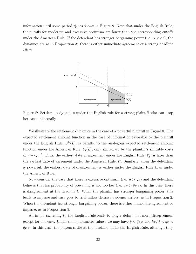
information until some period t∗E, as shown in Figure 8. Note that under the English Rule,

the cutoffs for moderate and excessive optimism are lower than the corresponding cutoffs

under the American Rule. If the defendant has stronger bargaining power (i.e. α < α∗), the

dynamics are as in Proposition 3: there is either immediate agreement or a strong deadline

effect.

Figure 8: Settlement dynamics under the English rule for a strong plaintiff who can drop

her case unilaterally

We illustrate the settlement dynamics in the case of a powerful plaintiff in Figure 8. The

expected settlement amount function in the case of information favorable to the plaintiff

under the English Rule, SEt (L), is parallel to the analogous expected settlement amount

function under the American Rule, St(L), only shifted up by the plaintiff’s shiftable costs

kP,S + cP,S t. Thus, the earliest date of agreement under the English Rule, t∗E, is later than

the earliest date of agreement under the American Rule, t∗. Similarly, when the defendant

is powerful, the earliest date of disagreement is earlier under the English Rule than under

the American Rule.

Now consider the case that there is excessive optimism (i.e. y > yE) and the defendant

believes that his probability of prevailing is not too low (i.e. qP > qP,E). In this case, there

is disagreement at the deadline t. When the plaintiff has stronger bargaining power, this

leads to impasse and case goes to trial unless decisive evidence arrives, as in Proposition 2.

When the defendant has stronger bargaining power, there is either immediate agreement or

impasse, as in Proposition 3.

All in all, switching to the English Rule leads to longer delays and more disagreement

except for one case. Under some parameter values, we may have y < qP,E and kP/J < qP <

qP,E. In this case, the players settle at the deadline under the English Rule, although they

38

would have disagreed under the American Rule. For example, if the plaintiff has stronger

bargaining power, there will be an impasse under the American Rule, but a strong deadline

effect under the English Rule.

8 Conclusion

Costly settlement delays and impasse are common in pretrial negotiations. A prominent

explanation for these delays is excessive optimism about the outcome of the trial. This has

been well established for the case of impasse in traditional static models of negotiation. In

this article, we develop a tractable dynamic model of negotiations in which the parties can

learn about the strength of their respective cases as negotiations go on. With our model, we

are able to analytically derive whether and when the parties reach an agreement, and how

the dynamics of such an agreement are affected by a variety of factors, such as the balance

of bargaining power between the two parties, the parties’ ability to commit, and the extent

of each party’s liability.

The underlying rationale for delay is as follows: the parties’ optimism about the trial

translates into optimism about the settlement amount that would be agreed upon if infor-

mation in their favor were to arrive. The parties wait without settling if and only if their

optimism about a future settlement exceeds their costs of waiting an additional day, and they

settle as soon as the cost of waiting outweighs their prospects for future gains. Therefore, the

dynamics of such strategic settlements are driven by the dynamics of the expected settlement

amount when the outcome of the trial is known. When optimism about a settlement that

would come due to an arrival of information, i.e. y(St(L)−St(NL)), exceeds the cost-benefit

ratio of waiting an additional period for information, R(t) ≈ c(t)λ(t)

, the parties choose to wait

rather than settle. By analyzing the effect of the various factors of the expected settlement

amount, we are able to understand the effects of different policies under consideration in

public discourse, in the presence of optimism. It is well known in the literature how different

factors may affect St(L). Thus, our model enables an analysis of how these factors may

affect agreement dynamics as well.

For example, under the baseline model with the “American Rule”, the difference in the

expected settlement amount St(L) − St(NL) increases as we go away from the deadline,

when the plaintiff has more bargaining power. In this case, the incentive to wait under

optimism also increases as we go away from the deadline, yielding straight-forward agreement

dynamics. If the level of optimism y is so excessive that the parties would not agree at the

39

deadline, then they will never agree prior to the deadline either and the negotiations will

end in impasse, unless decisive evidence arrives. This happens when the level of optimism

y exceeds the cutoff y, which equates the optimism about the trial outcome, Jy, with the

cost of going to trial, k. On the other hand, if the level of optimism is moderate so that y is

between y∗ and y, then the parties settle strategically at the deadline, but not before that.

This is because the level of optimism ySt(L) exceeds the effective cost of delaying negotiations

an additional day c(t)/λ(t). This deadline effect is a well known empirical regularity. If the

level of optimism is low, so that y < y∗, then the parties wait until the date t∗, at which

the effective cost of optimism is equal to the effective cost of waiting. By contrast, if the

defendant has more bargaining power, the settlement amount decreases as we go away from

the deadline, decreasing the incentive for the delay. This leads to a qualitatively different

set of agreement dynamics in which the parties either agree immediately, or they wait until

the deadline.

By the same token, we have shown how a policy change from the American Rule to

the English Rule would affect settlement delays. Such a reform is equivalent to adding the

plaintiff’s effective trial cost to the judgment amount. This causes the difference in expected

settlement amounts St(L)− St(NL) to be higher, thereby increasing the incentive for both

parties to delay. Consequently, such a reform would result in longer delays and higher rates

of impasse.

A Omitted Proofs and Technical Details

Proof of Lemma 1. We will use backward induction assuming that it has been revealed that

the defendant is liable. At any t, the defendant accepts a settlement offer S if and only if

S ≤ St+∆ (L) + cD∆. Then, if selected, the plaintiff offers the settlement amount St,P =

St+∆ (L) + cD∆. On the other hand, in responding to an offer S, the plaintiff accepts it if

S ≥ max {St+∆ (L)− cP∆, 0} ≡ St,D, rejects it and continues the negotiation if S < St,D

and St+∆ (L) ≥ cP∆, rejects and drop the case otherwise. Hence, if selected, the defendant

offers St,D. Thus, the settlement amount is

St (L) = αSt,P + (1− α)St,D =

{St+∆ (L) + αc∆− cP∆ if St+∆ (L) ≥ cP∆

αSt+∆ (L) + αcD∆ otherwise.

Now, if α ≥ α∗, as St (L) ≥ cP∆, we have that St (L) ≥ St+∆ (L) ≥ cP∆ for each t, and

thus we have St (L) = St+∆ (L) +αc∆− cP∆ throughout, for which the solution is as in (5).

Now assume α < α∗. Then, whenever St+∆ (L) ≥ cP∆, we have St (L) < St+∆ (L), and the

40

solution in (5) is decreasing in (t− t). The solution remains as in (5) provided that St+∆ (L)

remains above cP∆—until some t at which St+∆ (L) ≤ cP∆. But whenever St+∆ (L) ≤ cP∆,

we have

St (L) = α (St+∆ (L) + cD∆) ≤ αc∆ < α∗c∆ = cP∆.

Thus, for all t ≤ t, we have St+∆ (L) ≤ cP∆—and this case is excluded in the lemma.

We next present a simple general formula that determines when there is an agreement regime.

Fix an arbitrary date t0 and suppose that t1 is the earliest date with an agreement regime after

t0. If there is an arrival at some t ∈ (t0, t1], the parties reach an agreement. The expected value

of such a settlement for the plaintiff and the defendant is qPSt (L) and qDSt (L), respectively, as

the settlement value is zero when the information indicates no liability. Hence, the players have

optimistic beliefs about such a settlement, and the level of optimism is ySt (L). On the other hand,

if they agree at t1 without an arrival, there is no optimism or pessimism about such a settlement

because the value St1 (∅) of a settlement is known in equilibrium and the parties have identical

expectations about such a contingency. Hence, the total optimism about the future settlements is

Y (t0, t1) =∑

t∈T ∗,t0<t≤t1

P (t|t0)ySt (L) . (14)

This is the expected value of a settlement due to an arrival of information, multiplied by the

optimism level y. On the other hand, the expected total cost of waiting is

C (t0, t1) = e−λ(t1−t0)c (t1 − t0) +∑

t∈T ∗,t0<t≤t1

P (t|t0)c (t− t0) . (15)

Here, the first term is the cost c (t1 − t0) paid for waiting until t1 to settle, multiplied by the

probability that information does not arrive before t1, and the second term is the expected cost of

waiting if there is an arrival at a date in the interval between t0 and t1. Because of the constant

arrival rate, the cost adds up to

C (t0, t1) = R ·(1− e−λ(t1−t0)

), (16)

the cost-benefit ratio R = ∆c/(1− e−λ∆

)of waiting for information, normalized by the proba-

bility 1− e−λ(t1−t0) of arrival before the parties give up on waiting.

If there is no agreement regime after t0, we take t1 = t. In this case, we simply add e−λ(t−t0)yJ

to the optimism from future settlements to incorporate the optimism about the judge’s decision:

Y (t0, t) = e−λ(t−t0)yJ +∑

t∈T ∗,t0<t≤t1

P (t|t0)ySt (L) . (17)

41

We also include the litigation costs in the expected total cost:

C (t0, t) = e−λ(t−t0) [c (t− t0) + k] +∑

t∈T ∗,t0<t≤t1

P (t|t0)c (t− t0) . (18)

The next result states that there is an agreement regime at a given date if and only if the total

amount of optimism about future settlements does not exceed the expected total cost of waiting.

Lemma 6. There is an agreement regime at t0 if and only if

Y (t0, t1) ≤ C (t0, t1) (19)

where t1 is the earliest date with an agreement regime after t0 when there is such a date and it is

t otherwise.

Proof. Consider the case that there is an agreement regime at t1 (the other case is proved similarly).

The continuation value of the plaintiff is

Vt,P (∅) =∑

t∈T ∗,t0<t≤t1

P (t|t0)(qPSt (L)− cP (t− t0)) + e−λ(t1−t0) (St1 (∅)− cP (t1 − t0)) .

To see this note that, if there is an arrival at t, the parties reach an agreement where the settlement

is St (L) if the information indicates liability and 0 otherwise, yielding expected settlement payment

of qPSt (L) to the plaintiff. She also pays costs depending on the settlement date. Similarly,

Vt,D (∅) =∑

t∈T ∗,t0<t≤t1

P (t|t0)(−qDSt (L)− cD(t− t0)) + e−λ(t1−t0) (−St1 (∅)− cD (t1 − t0)) ,

where he expects to pay only qDSt (L) if there is an arrival at t. Adding up the two equations, we

obtain that Vt,P (∅) + Vt,D (∅) ≤ 0 if and only if∑t∈T ∗,t0<t≤t1

P (t|t0) [(ySt (L)− (cP + cD) (t− t0))] ≤ e−λ(t1−t0)(cP + cD) (t1 − t0) ,

as in the lemma.

Lemma 6 provides a simple cost-benefit analysis for determining the agreement regimes. In

particular, whether there is an agreement regime at a given date is independent of the settle-

ment amounts without an arrival. Using this fact, we can identify the dates with agreement and

disagreement regimes in a straightforward fashion, without computing the equilibrium settlements.

Our next result establishes the agreement dynamics for the powerful defendant case and im-

mediately implies Proposition 3. The function f (t0, t1) = E [St (L) |t0 < t ≤ t1] plays an impor-

tant role in this result. Note that f (t0, t1) is a convex combination of St0 (L) and f (t0 + ∆, t1).

Hence, f (t0, t1) is increasing in t0 when f (t0, t1) ≥ cP∆—because St (L) is increasing in t when

St+∆ (L) ≥ cP∆.

42

Proposition 7. Assume α < α∗. When y ≤ y, there is an agreement regime at every t ∈{0,∆, . . . , t∗∗, t} and a disagreement regime at every t with t∗∗ < t < t where

t∗∗ ≡ max {t ∈ T ∗|f (t, t) ≤ s∗} . (20)

When y > y, there is there is an agreement regime at every t ≤ t∗∗∗ and a disagreement regime at

every t with t > t∗∗∗ where

t∗∗∗ ≡ max{t ∈ T ∗|f(t, t) ≤ s∗∗(t)} (21)

and

s∗∗(t) = s∗ − e−λ(t−t)

1− e−λ(t−t) (J − k/y)

Proof. Lemma 2 directly implies that in equilibrium, either the players agree immediately or they

wait for the deadline. If there is a date t < t with an agreement regime, then by Lemma 2,

St+∆ (L) ≤ s∗. As α < α∗and s∗ > cP∆, this further implies that St+∆ (L) ≤ s∗ for each t ≤ t. As

there is an agreement regime at t, together with Lemma 2, this implies that there is an agreement

regime at each t ≤ t. In particular, there is an agreement regime at t = 0, and the players reach

an agreement immediately in equilibrium.

To prove the second statement, assume that y ≤ y, so that there is an agreement regime at t.

Then, one can show that, for any t0 ≥ t∗∗,

Y (t0, t) = yf (t0, t)(

1− e−λ(t−t0))

and

C (t0, t) = ys∗(

1− e−λ(t−t0)).

Hence, by Lemma 6, there is an agreement regime at t0 if and only if f (t0, t) ≤ s∗. In particular,

there is a disagreement regime at each t0 with t∗∗ < t0 < t, and there is an agreement regime at

t∗∗. The previous paragraph also implies then that there is an agreement regime at each t ≤ t∗∗.Finally, when y > y, there is a disagreement regime at t, and for each t0 ≥ t∗∗,

Y (t0, t) = yf (t0, t)(

1− e−λ(t−t0))

+ e−λ(t−t0)yJ

and

C (t0, t) = ys∗(

1− e−λ(t−t0))

+ e−λ(t−t0) [(c (t− t) + k)] .

Note that Y (t0, t) > C (t0, t) if and only if the inequality in (21) holds. Moreover, at any t > t∗∗∗,

we have f(t, t) > s∗∗(t), and there is disagreement. Similarly, there is an agreement regime at every

t ≤ t∗∗∗.

Proof of Lemma 2. This lemma was proved in the text and follows from Lemma 3.

43

Proof of Lemma 3. Consider any t. Without any information arrival, the continuation values of

the Plaintiff and the Defendant at t are

Vt,P (∅) = pΛ (t)St+∆ (L) + (1− Λ (t))Vt+∆,P (∅)− cP∆

Vt,D (∅) = −qΛ (t)St+∆ (L) + (1− Λ (t))Vt+∆,D (∅)− cD∆,

respectively. To see this, observe that there will be an arrival with probability Λ (t) until the next

period. According to the Plaintiff, with probability p the information will point to liability, leading

to settlement St+∆ (L); the settlement will be zero with the remaining probability 1 − p. With

probability 1 − Λ (t), there is no information arrival, and the continuation values are as at t + ∆,

minus the cost of waiting. By adding up these equalities, we obtain

Vt,P (∅) + Vt,D (∅) = yΛ (t)St+∆ (L) + (1− Λ (t)) (Vt+∆,P (∅) + Vt+∆,D (∅))− c∆.

Observe also that the sum of continuation values is always non-negative:

Vt+∆,P (∅) + Vt+∆,D (∅) ≥ 0;

it is positive if there is disagreement at t+ ∆ and zero if there is agreement at t+ ∆. Hence,

Vt,P (∅) + Vt,D (∅) ≥ yΛ (t)St+∆ (L)− c∆.

Now, if St+∆ (L) > c∆yΛ(t) , then yΛ (t)St+∆ (L) − c∆ > 0, showing that Vt,P (∅) + Vt,D (∅) > 0.

There is a disagreement regime at t in that case, proving the first part. To prove the second part,

observe that if there is agreement at t+ ∆, then Vt+∆,P (∅) + Vt+∆,D (∅) = 0, yielding

Vt,P (∅) + Vt,D (∅) = yΛ (t)St+∆ (L)− c∆.

If in addition St+∆ (L) ≤ c∆yΛ(t) , then yΛ (t)St+∆ (L)− c∆ ≤ 0, showing that there is an agreement

regime at t.

Proof of Lemma 4. As y is uniformly distributed on [0, 1], we can compute the distribution of t∗

from (10) as follows. By (10), for any t < t,

Ft∗ (t) = Pr{t∗ ≤ t} = Pr{y ≤ c/λ

(t− t)(α− α∗)c+ (J + αk − kP )} = β(t),

where the last equality is by substituting the values of A and B and by the fact that y is uniformly

distributed. At the deadline t, by Proposition 2, there is an agreement regime if y ≤ y, and there

is impasse otherwise. Therefore, Ft∗ (t) = y.

Proof of Lemma 5. As y and τA are independent, by definition,

Fτ∗(t) = Pr {min {t∗, τA} ≤ t}

= Pr {τA ≤ t}+ Pr {t∗ ≤ t}Pr {τA > t}

44

yielding the expression for Fτ∗(t) in the proposition. It is straightforward to obtain the expressions

for the density and the hazard rate from Fτ∗(t).

Proof of Proposition 4. Take any t < t. From Lemma 5,

∂fτ∗(t)

∂t= λ

(−λe−λt

[(α− α∗)β(t)2 − β(t) + 1

]+ e−λt

[2 (α− α∗)β(t)β′(t)− β′(t)

]).

Hence fτ∗(t) is decreasing if and only if the above expression is negative:

−λ[(α− α∗)β(t)2 − β(t) + 1

]+[2 (α− α∗)β(t)β′(t)− β′(t)

]< 0.

This further simplifies to

λ[2 (α− α∗)2 β(t)3 − 2 (α− α∗)β(t)2 + β(t)− 1

]< 0.

This is indeed the case when (α− α∗) is positive and β(t) ∈ [0, 1]. Indeed, varying β ∈ [0, 1]

and α − α∗ ≥ 0, the only root of λ[2 (α− α∗)2 β3 − 2 (α− α∗)β2 + β − 1

]is given by β = 1 and

α − α∗ = 0. As the above expression is −λ for β = 0, this shows that it is negative at all feasible

values of α− α∗ and β.

Now, consider the hazard rate, Hτ∗(t). One can compute that

∂Hτ∗(t)

∂t=λ2 (α− α∗)2 β(t)3

(1− β(t))2 +λ2 (α− α∗)2 β(t)3

(1− β(t))> 0.

(Both terms are positive because β > 0 and α− α∗ > 0. )

45

References

S Nageeb M Ali. Waiting to Settle: Multilateral Bargaining with Subjective Biases. Journal of

Economic Theory, 130:109–137, 2006.

Linda Babcock and George Loewenstein. Explaining Bargaining Impasse : The Role of Self-Serving

Biases. The Journal of Economic Perspectives, 11(1):109–126, 1997.

Linda Babcock, George Loewenstein, Samuel Issacharoff, and Colin Camerer. Biased judgments of

fairness in bargaining. The American Economic Review, 85(5):1337–1343, 1995.

Linda Babcock, Xianghong Wang, and George Loewenstein. Choosing the wrong pond: Social

comparisons in negotiations that reflect a self-serving bias. The Quarterly Journal of Economics,

111(1):1–19, 1996.

Lucian Arye Bebchuk. Litigation and Settlement under Imperfect Information. The RAND Journal

of Economics, 15(3):404, 1984.

Lucian Arye Bebchuk. A New Theory concerning the Credibility and Success of Threats to. The

Journal of Legal Studies, 25(1):1–25, 1996.

Jack Fanning. Reputational bargaining and deadlines. Econometrica, 84(3):1131–1180, 2016.

Henry S Farber and Harry C Katz. Interest Arbitration , Outcomes , and the Incentive to Bargain.

ILR Review, 33(1):55–63, 1979.

Gary M Fournier and Thomas W Zuehlke. The Timing of Out-of-Court Settlements. RAND

Journal of Economics, 27(2):310–321, 1996.

Jane Goodman-Delahunty, Maria Hartwig, and Elizabeth F Loftus. Insightful or Wishful : Lawyers’

Ability to Predict Case Outcomes. Psychology, Public Policy, and Law, 16(2):133–157, 2010.

James W Hughes and Edward A Snyder. Litigation and Settlement under the English and American

Rules: Theory and Evidence, 1995.

Daniel Kessler. Institutional Causes of Delay in the Settlement of Legal Disputes. Journal of Law,

Economics, & Organization, 12(2):29, 1996.

William M Landes. An Economic Analysis of the Courts. Journal of Law and Economics, 14(1):

61–107, 1971.

Robert M Lloyd. Pennzoil v. texaco, twenty years after: Lessons for business lawyers. Transactions:

Tenn. J. Bus. L., 6:321, 2004.

46

George Loewenstein, Samuel Issacharoff, Colin Camerer, and Linda Babcock. Self-serving assess-

ments of fairness and pretrial bargaining. The Journal of Legal Studies, 22(1):135–159, 1993.

Elizabeth F Loftus and Willem A Wagenaar. Lawyers’ Predictions Of Success. Jurimetrics, 28(4):

437–453, 1988.

Ching-to Albert Ma and Michael Manove. Bargaining with Deadlines and Imperfect Agent Control.

Econometrica, 61:1313–1339, 1993.

Marijke Malsch. Advocaten voorspellen de uitkomst van hun zaken. Swets & Zeitlinger, Amsterdam,

1990.

Robert Mnookin and Robert Wilson. Rational Bargaining and Market Efficiency: Understanding

Pennzoil v. Texaco. Virginia Law Review, 75(2):295–334, 1989.

Margaret A Neale and Max H Bazerman. The Role of Perspective-Taking Ability in Negotiating

under Different Forms of Arbitration. Industrial and Labor Relations Review, 36(3), 1983.

Richard A Posner. The Behavior of Administrative Agencies. The Journal of Legal Studies, 1(2):

305–347, 1972.

George L. Priest and Benjamin Klein. The Selection of Disputes for Litigation. The Journal of

Legal Studies, 13(1):1–55, 1984.

Jennifer F Reinganum and Louis L Wilde. Settlement, litigation, and the allocation of litigation

costs. RAND Journal of Economics, 17(4):557–566, 1986.

Douglas Rennie. Rule 82 & Tort Reform: an Empirical Study of the Impact of Alaska’s English

Rule on Federal Civil Case Filings. Alaska Law Review, pages 1–34, 2012.

Ae Roth, Jk Murnighan, and Francoise Schoumaker. The deadline effect in bargaining: Some

experimental evidence. The American Economic Review, 78(4):806–823, 1988.

Alvin Roth and Axel Ockenfels. Last-Minute Bidding and the Rules for Ending Second-Price

Auctions: Evidence from eBay and Amazon Auctions on the Internet. American Economic

Review, 92:1093–1103, 2002.

Steven Shavell. Suit, Settlement, and Trial: A Theoretical Analysis under Alternative Methods for

the Allocation of Legal Costs. Journal of Legal Studies, 11(1):55–81, 1982.

Alp Simsek and Muhamet Yildiz. Durability, Deadline, and Election Effects in Bargaining. Working

Paper, 2015.

47

E A Snyder and J W Hughes. The English Rule for Allocating Legal Costs: Evidence Confronts

Theory. Journal of Law, Economics, and Organization, 6(2):345–380, 1990.

Kathryn E Spier. The dynamics of pretrial negotiation. The Review of Economic Studies, 59(1):

93–108, 1992.

John Thanassoulis. Optimal stalling when bargaining. Journal of Economic Dynamics and Control,

34(2):101–120, 2010.

Yasutora Watanabe. Learning and Bargaining in Dispute Resolution: Theory and Evidence from

Medical Malpractice Litigation. Working Paper, 2006.

G R Williams. Legal Negotiations and Settlement. West Publishing, St. Paul, MN., 1983.

Muhamet Yildiz. Bargaining without a Common Prior — An Agreement Theorem. Econometrica,

71:793–811, 2003.

Muhamet Yildiz. Waiting to persuade. Quarterly Journal of Economics, 119(1):223–249, 2004.

Muhamet Yildiz. Bargaining with Optimism. Annual Review of Economics, 3:451–478, 2011.

48

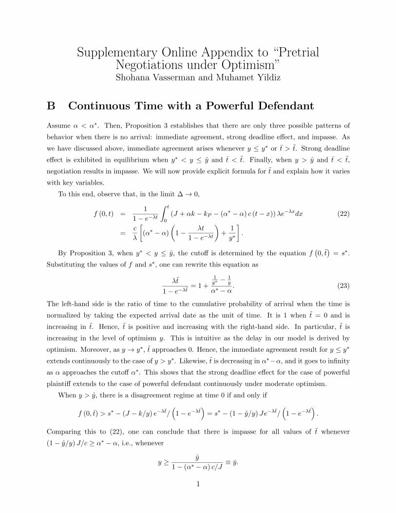
Supplementary Online Appendix to “PretrialNegotiations under Optimism”Shohana Vasserman and Muhamet Yildiz

B Continuous Time with a Powerful Defendant

Assume α < α∗. Then, Proposition 3 establishes that there are only three possible patterns of

behavior when there is no arrival: immediate agreement, strong deadline effect, and impasse. As

we have discussed above, immediate agreement arises whenever y ≤ y∗ or t > t. Strong deadline

effect is exhibited in equilibrium when y∗ < y ≤ y and t < t. Finally, when y > y and t < t,

negotiation results in impasse. We will now provide explicit formula for t and explain how it varies

with key variables.

To this end, observe that, in the limit ∆→ 0,

f (0, t) =1

1− e−λt

∫ t

0(J + αk − kP − (α∗ − α) c (t− x))λe−λxdx (22)

=c

λ

[(α∗ − α)

(1− λt

1− e−λt

)+

1

y∗

].

By Proposition 3, when y∗ < y ≤ y, the cutoff is determined by the equation f(0, t)

= s∗.

Substituting the values of f and s∗, one can rewrite this equation as

λt

1− e−λt= 1 +

1y∗ −

1y

α∗ − α. (23)

The left-hand side is the ratio of time to the cumulative probability of arrival when the time is

normalized by taking the expected arrival date as the unit of time. It is 1 when t = 0 and is

increasing in t. Hence, t is positive and increasing with the right-hand side. In particular, t is

increasing in the level of optimism y. This is intuitive as the delay in our model is derived by

optimism. Moreover, as y → y∗, t approaches 0. Hence, the immediate agreement result for y ≤ y∗

extends continuously to the case of y > y∗. Likewise, t is decreasing in α∗−α, and it goes to infinity

as α approaches the cutoff α∗. This shows that the strong deadline effect for the case of powerful

plaintiff extends to the case of powerful defendant continuously under moderate optimism.

When y > y, there is a disagreement regime at time 0 if and only if

f (0, t) > s∗ − (J − k/y) e−λt/(

1− e−λt)

= s∗ − (1− y/y) Je−λt/(

1− e−λt).

Comparing this to (22), one can conclude that there is impasse for all values of t whenever

(1− y/y) J/c ≥ α∗ − α, i.e., whenever

y ≥ y

1− (α∗ − α) c/J≡ y.

1

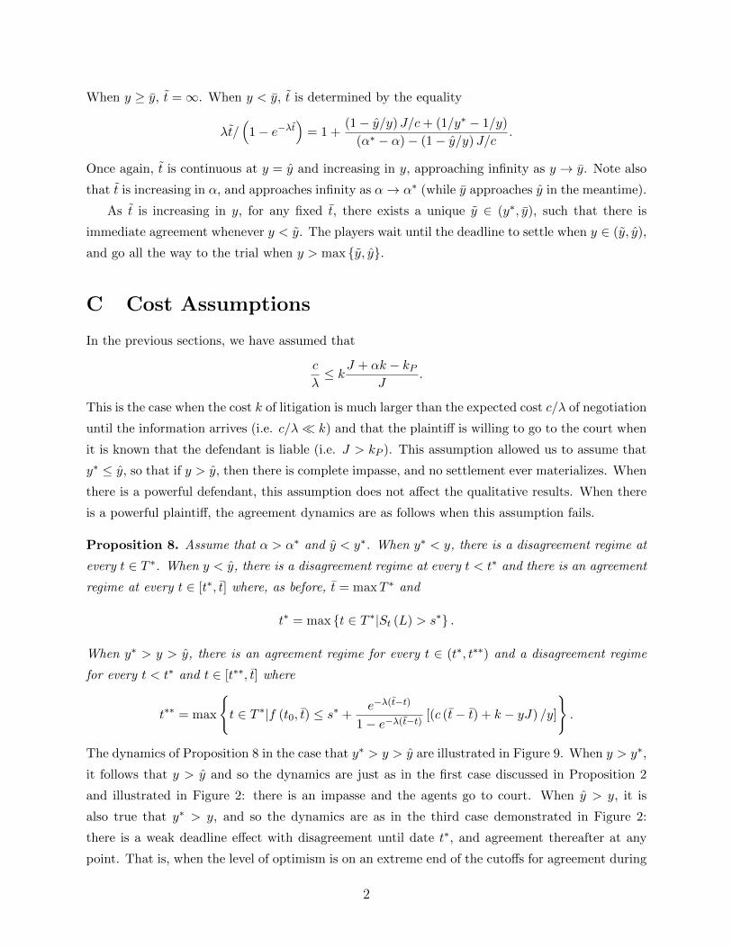
When y ≥ y, t =∞. When y < y, t is determined by the equality

λt/(

1− e−λt)

= 1 +(1− y/y) J/c+ (1/y∗ − 1/y)

(α∗ − α)− (1− y/y) J/c.

Once again, t is continuous at y = y and increasing in y, approaching infinity as y → y. Note also

that t is increasing in α, and approaches infinity as α→ α∗ (while y approaches y in the meantime).

As t is increasing in y, for any fixed t, there exists a unique y ∈ (y∗, y), such that there is

immediate agreement whenever y < y. The players wait until the deadline to settle when y ∈ (y, y),

and go all the way to the trial when y > max {y, y}.

C Cost Assumptions

In the previous sections, we have assumed that

c

λ≤ kJ + αk − kP

J.

This is the case when the cost k of litigation is much larger than the expected cost c/λ of negotiation

until the information arrives (i.e. c/λ� k) and that the plaintiff is willing to go to the court when

it is known that the defendant is liable (i.e. J > kP ). This assumption allowed us to assume that

y∗ ≤ y, so that if y > y, then there is complete impasse, and no settlement ever materializes. When

there is a powerful defendant, this assumption does not affect the qualitative results. When there

is a powerful plaintiff, the agreement dynamics are as follows when this assumption fails.

Proposition 8. Assume that α > α∗ and y < y∗. When y∗ < y, there is a disagreement regime at

every t ∈ T ∗. When y < y, there is a disagreement regime at every t < t∗ and there is an agreement

regime at every t ∈ [t∗, t] where, as before, t = maxT ∗ and

t∗ = max {t ∈ T ∗|St (L) > s∗} .

When y∗ > y > y, there is an agreement regime for every t ∈ (t∗, t∗∗) and a disagreement regime

for every t < t∗ and t ∈ [t∗∗, t] where

t∗∗ = max

{t ∈ T ∗|f (t0, t) ≤ s∗ +

e−λ(t−t)

1− e−λ(t−t) [(c (t− t) + k − yJ) /y]

}.

The dynamics of Proposition 8 in the case that y∗ > y > y are illustrated in Figure 9. When y > y∗,

it follows that y > y and so the dynamics are just as in the first case discussed in Proposition 2

and illustrated in Figure 2: there is an impasse and the agents go to court. When y > y, it is

also true that y∗ > y, and so the dynamics are as in the third case demonstrated in Figure 2:

there is a weak deadline effect with disagreement until date t∗, and agreement thereafter at any

point. That is, when the level of optimism is on an extreme end of the cutoffs for agreement during

2

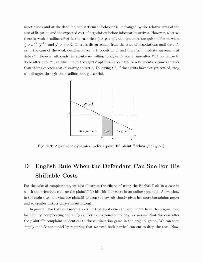
negotiations and at the deadline, the settlement behavior is unchanged by the relative sizes of the

cost of litigation and the expected cost of negotiation before information arrives. However, whereas

there is weak deadline effect in the case that y > y > y∗, the dynamics are quite different whencλ > k J+αk−kP

J and y∗ > y > y. There is disagreement from the start of negotiations until date t∗,

as in the case of the weak deadline effect in Proposition 2, and there is immediate agreement at

date t∗. However, although the agents are willing to agree for some time after t∗, they refuse to

do so after date t∗∗, at which point the agents’ optimism about future settlements becomes smaller

than their expected cost of waiting to settle. Following t∗∗, if the agents have not yet settled, they

will disagree through the deadline, and go to trial.

Figure 9: Agreement dynamics under a powerful plaintiff when y∗ > y > y.

D English Rule When the Defendant Can Sue For His

Shiftable Costs

For the sake of completeness, we also illustrate the effects of using the English Rule in a case in

which the defendant can sue the plaintiff for his shiftable costs in an online appendix. As we show

in the main text, allowing the plaintiff to drop the lawsuit simply gives her more bargaining power

and so creates further delays in settlement.

In general, the trial and negotiations for that legal case can be different from the original case

for liability, complicating the analysis. For expositional simplicity, we assume that the case after

the plaintiff’s complaint is identical to the continuation game in the original game. We can then

simply modify our model by requiring that we need both parties’ consent to drop the case. Now,

3

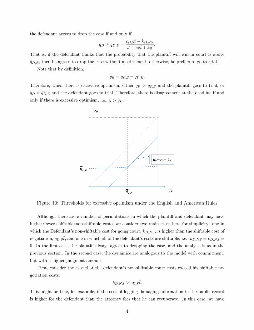
the defendant agrees to drop the case if and only if

qD ≥ qD,E =cD,S t− kD,NSJ + cS t+ kS

.

That is, if the defendant thinks that the probability that the plaintiff will win in court is above

qD,E , then he agrees to drop the case without a settlement; otherwise, he prefers to go to trial.

Note that by definition,

yE = qP,E − qD,E .

Therefore, when there is excessive optimism, either qP > qP,E and the plaintiff goes to trial, or

qD < qD,E and the defendant goes to trial. Therefore, there is disagreement at the deadline if and

only if there is excessive optimism, i.e., y > yE .

Figure 10: Thresholds for excessive optimism under the English and American Rules

Although there are a number of permutations in which the plaintiff and defendant may have

higher/lower shiftable/non-shiftable costs, we consider two main cases here for simplicity: one in

which the Defendant’s non-shiftable cost for going court, kD,NS , is higher than the shiftable cost of

negotiation, cD,S t, and one in which all of the defendant’s costs are shiftable, i.e., kD,NS = cD,NS =

0. In the first case, the plaintiff always agrees to dropping the case, and the analysis is as in the

previous section. In the second case, the dynamics are analogous to the model with commitment,

but with a higher judgment amount.

First, consider the case that the defendant’s non-shiftable court costs exceed his shiftable ne-

gotiation costs:

kD,NS > cD,S t.

This might be true, for example, if the cost of logging damaging information in the public record

is higher for the defendant than the attorney fees that he can recuperate. In this case, we have

4

qD,E < 0, and the defendant does not sue if the plaintiff decides to drop the case. Moreover,

we have qP,E = yE − qD,E > yE , and hence there is disagreement at the deadline if and only if

y > yE , mirroring the dynamics under the American Rule. When the case involves a powerful

plaintiff (with α > α∗), there is impasse when optimism is excessive (i.e., y > yE), there is a strong

deadline effect when optimism is moderate (i.e., y∗E < y < yE), and there is weak deadline effect

otherwise. When the case involves a powerful defendant, there is either immediate agreement, a

strong deadline effect, or impasse, depending on the level of optimism and t.

Now assume that all costs are shiftable: k = kS and c = cS . In this case, one of the parties will

always want to go to trial, and thus the case will not dropped once it is filed—as is the case under

the American Rule with commitment. If there is an arrival of decisive evidence that the defendant

is not liable, then the parties settle with settlement amount27

SE,Ct (NL) = α (k + c (t− t))− (k + ct) + cP t.

This amount reflects the fact that the plaintiff is responsible for paying all of the costs of negotiations

– both the costs that have already incurred at the time of settlement and the costs averted by

discontinuing negotiations – and that she has already incurred the cost cP t. Similarly, if there is

decisive evidence that the defendant is liable, then the parties settle with settlement amount

SE,Ct (L) = α (k + c (t− t)) + J + kP + cP t− (kP + cP (t− t)) .

As in the analysis under the American Rule with commitment, the difference between the two

settlement amounts in this case is equal to the amount contested in the court:

SE,Ct (L)− SE,Ct (NL) = J + k + ct.

Under the American Rule, the contested amount was only J . As under the American Rule with

commitment, there is either immediate agreement, or strong deadline effect, or impasse, depending

on whether optimism is low (i.e. y ≤ y∗E,C), moderate (i.e. y∗EC < y ≤ yE), or excessive (i.e.,

y ≤ yE), where the lower cutoff for moderate optimism y∗EC is determined by equating the difference

SE,Ct (L)− SE,Ct (NL) to the critical level s∗ in the baseline model:

y∗EC =c∆

Λ (J + kS + cS t).

The corresponding cutoff was c∆ΛJ under the American rule with commitment. All in all, when

all costs are shiftable, the English rule is equivalent to the American Rule with commitment and

increased judgment amount J + k + ct, leading to more delay and disagreement.

27Note that the plaintiff might wish to drop the case when this happens, but the defendant will not agree.

5