Preston, T. C., & Reid, J. P. (2015). Angular scattering of light by ahomogeneous spherical particle in a zeroth-order Bessel beam and itsrelationship to plane wave scattering. Journal of the Optical Society ofAmerica, A: Optics, Image Science and Vision, 32(6), 1053-1062. DOI:10.1364/JOSAA.32.001053

Peer reviewed version

Link to published version (if available):10.1364/JOSAA.32.001053

Link to publication record in Explore Bristol ResearchPDF-document

University of Bristol - Explore Bristol ResearchGeneral rights

This document is made available in accordance with publisher policies. Please cite only the publishedversion using the reference above. Full terms of use are available:http://www.bristol.ac.uk/pure/about/ebr-terms

Angular scattering of light by a homogeneous spherical

particle in a zeroth-order Bessel beam and its relationship

to plane wave scattering

April 11, 2015

Thomas C. Preston*a and Jonathan P. Reidb

aDepartment of Atmospheric and Oceanic Sciences

and Department of Chemistry, McGill University,

805 Sherbrooke Street West, Montreal, QC, Canada H3A 0B9

bSchool of Chemistry, University of Bristol,

Cantock’s Close, Bristol, UK, BS8 1TS

submitted to the Journal of the Optical Society of America A

7 Figures, 1 Table and 18 manuscript pages

* Thomas C. Preston

e-mail: thomas.preston@mcgill.com

Abstract

The angular scattering of light from a homogeneous spherical particle in a zeroth-order Bessel

beam is calculated using generalized Lorenz-Mie theory. We investigate the dependence of the

angular scattering on the semi-apex angle of the Bessel beam and discuss the major features of

the resulting scattering plots. We also compare Bessel beam scattering to plane wave scattering

and provide criterion for when the difference between the two cases can be considered negligible.

Finally, we discuss a method for characterizing spherical particles using angular light scattering.

This work is useful to researchers who are interested in characterizing particles trapped in optical

beams using angular dependent light scattering measurements.

OCIS Codes: (010.1110) Aerosols; (290.3030) Index measurements; (290.4020) Mie theory

1

1 Introduction

An accurate understanding of elastic light scattering by particles is important in many scientific

fields. For over a hundred years, Lorenz-Mie theory (LMT)1,2 has provided the foundation for

qualitative and quantitative insight into a wide range of optical phenomena involving spherical

particles,3–7 among which the angular scattering of light has been one of the most important.8,9

Computer code implementing LMT has been around for many decades (e.g. see Ref. 9, p. 477)

and researchers can now calculate Mie coefficients in a computationally efficient manner.

However, even when restricted to the scattering of light by a spherical particle, calculations

performed using the classical LMT may not accurately model experimental measurements. One

of the most the common deficiencies of LMT is that the plane wave used in its formulation may

not be suitable in describing the incident beam for the system of interest. This problem has been

studied extensively, in particular for light scattering involving spherical particles in a Gaussian

beam, and has led to the development of two popular theories which extend LMT to the case

of an arbitrarily shaped beam.10–17 These theories are mathematically equivalent and in both

cases beam-shape coefficients are used to decompose the incident beam into partial waves.14

Generalized Lorenz-Mie theory (GLMT)11,14–17 will be used throughout this work, although

many of the calculations were also verified using the theory of Barton et al.10,12,13 (as expected,

results from both theories were identical).

Optical Bessel beams have several properties that make their use in the manipulation and

control of micron and sub-micron particles attractive: pseudo-nondiffracting, strong confine-

ment forces in the transverse plane, and self-reconstruction.18–22 In the field of aerosol science,

Bessel beams are very appealing for the study of single aerosol particles and instrumentation

2

incorporating such beams has been recently demonstrated.23–29 However, there remains the

need for an approach to accurately characterize a particle once it has been trapped in such a

beam. For a homogeneous spherical particle the radius and refractive index must be accurately

determined. Whispering gallery modes that appear in cavity enhanced spectra are well-suited

for this task,30,31 but for sub-micron particles the spacing of these modes is often so large that

the number of observable modes may be insufficient to simultaneously fit the refractive index

and radius. While cavity enhanced Raman scattering has the requirement that the Raman

bands are spectrally broad enough to contain an adequate number of whispering gallery modes,

cavity enhanced fluorescence also has the limitation that particles will typically need to be

doped with a dye and are susceptible to photobleaching.

In contrast, angular dependent measurements of elastic light scattering are not restricted

in the above ways and can readily be made to determine the size of a sub-micron particle in

an optical Bessel trap.23–29 Such scattering will depend not only on radius and refractive index

but also, in general, on the shape of the Bessel beam. Therefore, using LMT to model the

scattering may not satisfactorily reproduce experimental results. Several groups have provided

expressions for the beam-shape coefficients for a Bessel beam20,32–34 and, in particular, the

work of Taylor and Love should be highlighted. These authors derived analytical expressions

for the beam-shape coefficients that do not contain any integrals and are valid outside of the

paraxial approximation.32 However, actual scattering calculations for a homogeneous sphere in

a Bessel beam have been limited. Mitri published reports on light scattering of both zeroth-

and higher-order Bessel beams35,36 and, more recently, Li et al. used a non-paraxial description

of a zeroth-order Bessel beam to study light scattering by a homogeneous sphere.34 None of this

work, though, considered systems that are relevant to the aerosol optical trapping discussed

3

above. Beyond the work on homogeneous spheres, elastic scattering of a zeroth-order optical

Bessel beam from particles with anisotropic optical properties37 and particles with a core-shell

structure38 have also recently been investigated.

Here, we focus on the angular dependent scattering of light by a homogeneous sphere in

an optical zeroth-order Bessel beam. First, we give an overview of the angular dependent

scattering as a function of the semi-apex angle of the Bessel beam (Section 3.1). Following that,

we discuss systems of experimental interest to aerosol science and how the angular dependent

scattering of a Bessel beam compares to that of a plane wave (Section 3.2). Finally, the

suitability of approximating Bessel beam scattering with plane wave scattering for the purpose

of characterizing spherical particles is examined (Section 3.3) and a new method for fitting both

the radius and refractive index of a spherical particle is presented (Section 3.4).

4

2 Theory

In the non-paraxial (vectorial) description of a zeroth-order Bessel beam, the electric and mag-

netic fields (E and H) of the incident beam can be written as20–22,39

E(r) = E0e−ikzz

[J0(k⊥ρ) + β2J2(k⊥ρ)cos 2φ]x

β2J2(k⊥ρ)sin 2φ y

i2βJ1(k⊥ρ)cosφ z

, (1)

H(r) = H0e−ikzz

β2J2(k⊥ρ)sin 2φ x

[J0(k⊥ρ)− β2J2(k⊥ρ)cos 2φ]y

i2βJ1(k⊥ρ)sinφ z

. (2)

For a Bessel beam of wavenumber k and semi-apex angle θ0, the longitudinal and transverse

wavenumbers are kz = k cos θ0 and k⊥ = k sin θ0, respectively (Fig. 1). Additionally, β =

sin θ0/(1 + cos θ0), ρ =√x2 + y2, and φ = arctan (y/x). The relationship between the field

amplitudes E0 and H0 is E0/H0 =√µ/ε where ε is the permittivity and µ is the permeability

of the medium. The time dependent factor of eiωt associated with the fields is omitted in this

work. Finally, x, y, and z are unit vectors in the cartesian coordinate system.

Scattering calculations were performed using GLMT.11,14–17 The transverse electric (gml )TE

and transverse magnetic (gml )TM beam-shape coefficients can be defined as two-dimensional

integrals:14

(gml )TE =−1

4π(il−1)

kr

jl(kr)

(l − |m|)!(l + |m|)!

∫ 2π

0

∫ π

0

(Hrad(r, θ, φ)/H0)P|m|l (cos θ)e−imφsin θdθdφ, (3)

(gml )TM =−1

4π(il−1)

kr

jl(kr)

(l − |m|)!(l + |m|)!

∫ 2π

0

∫ π

0

(Erad(r, θ, φ)/E0)P|m|l (cos θ)e−imφsin θdθdφ, (4)

where Erad and Hrad are the radial components of the incident fields, jl are spherical Bessel

functions, P|m|l are associated Legendre polynomials, and r is the radius at which integrals are

evaluated. Eqs. 3 and 4 were evaluated numerically using r = (l + 1/2)/k.33

5

In GLMT, the scattering amplitudes S1 and S2 can be written as11,14

S1(θ, φ) =∞∑l=1

l∑m=−l

2l + 1

l(l + 1)[(gml )TMalmπ

|m|l (θ) + i(gml )TEblτ

|m|l (θ)]eimφ, (5)

S2(θ, φ) =∞∑l=1

l∑m=−l

2l + 1

l(l + 1)[i(gml )TEblmπ

|m|l (θ) + (gml )TMalτ

|m|l (θ)]eimφ, (6)

where al and bl are the Mie scattering coefficients (Ref. 9, p. 101)

al =nψl(nα)ψ′l(α)− ψl(α)ψ′l(nα)

nψl(nα)ξ′l(α)− ξl(α)ψ′l(nα), (7)

bl =ψl(nα)ψ′l(α)− nψl(α)ψ′l(nα)

ψl(nα)ξ′l(α)− nξl(α)ψ′l(nα), (8)

and π|m|l and τ

|m|l are the angular functions14

π|m|l (θ) =

P|m|l (cos θ)

sin θ, (9)

τ|m|l (θ) =

d

dθP|m|l (cos θ). (10)

In Eqs. 7 and 8, the relative refractive index is n = ns/n0 where ns is the, in general, complex

refractive index of the sphere and n0 is the refractive index of the medium, the size parameter

is α = ka where a is the radius of the sphere, and the functions ξl = ψl − iχl, ψl, and χl

are Ricatti-Bessel functions. The infinite series in Eqs. 5 and 6 were truncated at the integer

closest to α + 4α1/3 + 2 during all calculations (Ref. 9, p. 477).

Following Bohren and Huffman (Ref. 9, p. 113), parallel (i‖) and perpendicular (i⊥) func-

tions of the scattered irradiance per unit incidence irradiance (a dimensionless quantity) are

defined using the scattering amplitudes (Eqs. 5 and 6) and a consideration of the polarization

of the incident Bessel beam (Eqs. 1 and 2)

i‖(θ) = |S2(θ, φ = 0◦)|2, (11)

6

i⊥(θ) = |S1(θ, φ = 90◦)|2. (12)

In these equations the angle φ has been chosen so that the Bessel beam described by Eqs. 1 and

2 will be polarized either parallel (Eq. 11) or perpendicular (Eq. 12) to the scattering plane.

The scattering planes associated with i‖ and i⊥ are shown in Fig. 2a and b, respectively.

7

3 Results and Discussion

3.1 General features of Bessel beam scattering

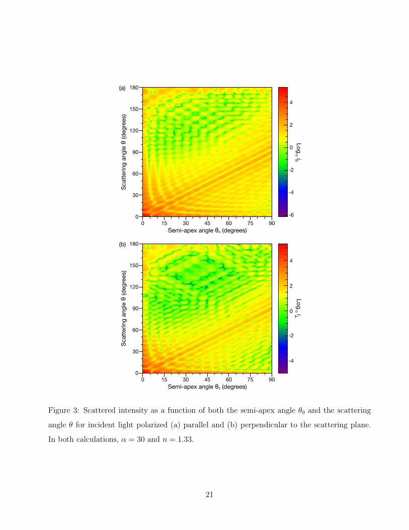
Fig. 3 shows the angular scattered irradiance, the parallel and perpendicular scattering com-

ponents, for a sphere with α = 30 and n = 1.33 in a Bessel beam. The scattering is plotted

as a function of both θ and θ0. In all cases here, spheres were centred on the propagation axis

of a Bessel beam. The justification for this choice is that this is where the potential energy of

the sphere in a zeroth-order Bessel beam will be at its global minimum19,22,26,40 and it should

therefore be the most relevant position for practical applications.

The most distinctive feature of both the parallel and perpendicular polarization plots is

the intense ridge of scattering that begins at θ = θ0 = 0◦, cuts across the plots in a nearly

straight line, and ends at θ = θ0 = 90◦. To explore these ridges further, vertical slices of Fig.

3a and b were taken at a constant θ0, generating multiple plots that were only a function of θ.

Examining the angles of maxima in these slices, a peak always occurred at θ ≈ θ0 except for

small θ0. This peak is always one of the most intense maxima in a vertical slice and is often

a global maximum at large θ0. In the classical LMT, one would not expect a peak other than

at θ = 0◦, the forward scattering direction, to be the strongest in an angular scattering plot.

This is because the scattering of a plane wave by a sphere will be by far the most intense in the

forward direction, particularly for large size parameters (see Ref. 9, p. 115). While we are not

dealing with plane wave illumination here, this result from LMT can provide an intuitive basis

for understanding the Bessel beam scattering. A common description of a Bessel beam is that

of a superposition of plane waves propagating on a cone with a semi-apex angle θ0 (Fig. 1).41

Thus, the forward direction for such plane waves is not θ = 0◦ but rather θ = θ0. With this

8

description and a consideration of scattering results from LMT, it therefore seems reasonable

to expect that the scattering of a sphere by a Bessel beam would be very intense at θ ≈ θ0.

The above results are not consistent with results recently presented by Li et al.34 There,

a similar trend was observed, but only for calculations where θ0 < 42◦. At higher angles, the

ridge was no longer located at θ ≈ θ0 and instead was found at θ < θ0. The origin of the

discrepancy between our results and those of Li et al. is the manner in which the calculations

were performed. Li et al. derived an analytical formula for the beam-shape coefficients by

solving Eqs. 3 and 4 with the fields in Eqs. 1 and 2 using the integral localized approximation.

Here, such an approximation was not used and Eqs. 3 and 4 were instead integrated numerically.

During testing we found that the beam-shape coefficients of Li et al. did not agree with the

beam-shape coefficients found through numerical integration for cases outside of the paraxial

limit. Therefore, there is most likely a problem with the beam-shape coefficients presented in

Ref. 34 and we recommend that their use be avoided.

A second feature of Fig. 3 is the undulation in scattered irradiance that occurs throughout

both plots. For instance, these intensity variations lead to a checkerboard type pattern in the

rectangular region of θ0 = 25 to 50◦ and θ = 130 to 155◦ in Fig. 3a. Intensity undulations

with similar periodicities are seen at all angles in both plots although they do not always form

such visually distinct patterns. A vertical slice at any θ0 always generates a scattering plot in θ

that contains maxima and minima. Therefore, regardless of θ0, it should always be possible to

determine the size of a particle using angular scattering. It is also interesting to note that taking

a horizontal slice at a fixed θ and generating a scattering plot as a function of θ0 would contain

intensity undulations with similar periodicities to those of the vertical slices. As a result, it

should also be possible to determine particle size by measuring the scattering at a fixed θ while

9

θ0 is varied. Such a measurement would be impractical with current instrumentation and it is

much easier to take measurements over a wide range of θ at a fixed θ0. These measurements as

a function of θ0 will not be discussed any further here.

3.2 Comparison between plane wave and Bessel beam scattering

Angular scattering plots are shown in Fig. 4 for spheres with n = 1.33 and at several different

size parameters α in Bessel beams with various θ0. These calculations were performed for

polarizations both parallel and perpendicular to the scattering plane. Of the five different θ0

chosen in Fig. 4, one gives results that are identical to plane wave scattering (θ0 = 0◦) while

the others cover the range typically used in aerosol optical Bessel traps (except θ0 = 30◦, which

is considerably larger than the maximum θ0 that has been used).23–29

Our analysis will focus on the conditions under which the scattering in a Bessel beam

deviates significantly from that of a plane wave. For small θ0, the first intensity minimum

of the non-paraxial zeroth-order Bessel beam will occur approximately at the dimensionless

parameter

r0 =2.40483

sin θ0, (13)

which corresponds to the first root of the zeroth-order Bessel function. The parameter r0 = kρ0

where ρ0 is the radial distance between the centre of the beam and the first intensity minimum,

which is commonly referred to as the central core size of a zeroth-order Bessel beam.19,42 The

parameter r0 is used here to define a scaled size γ = α/r0. As γ increases from zero to one, the

size parameter of the sphere approaches the first intensity minimum of the Bessel beam and it

is expected that the associated angular scattering will deviate significantly from that of a plane

wave.

10

Pearson’s correlation coefficients c were calculated between the angular scattering of a plane

wave (θ0 = 0◦) and the angular scattering of Bessel beams with various θ0. For a data set

containing N pairs (xi, yi) the correlation coefficient is

c =N

∑xiyi −

∑xi

∑yi√

N∑x2i − (

∑xi)2

√N

∑y2i − (

∑yi)2

. (14)

In the analysis here, each (xi, yi) consists of the scattered intensity of the plane wave and the

Bessel beam at the same angle. The set (x1, y1), (x2, y2), . . . , (xN , yN) spans the angular range

of interest.

Table 1 lists the correlations for all of the θ0 6= 0◦ plots shown in Fig. 4 with their cor-

responding θ0 = 0◦ (plane wave) plot. In the following discussion, a value of c = 0.99900 is

chosen to be the lower limit at which angular scattering for the Bessel system is no longer well

described by plane wave scattering. In Fig. 4, pairs of curves whose c is below this limit have

shapes that are easy to distinguish visually from that of a plane wave as they contain shifts in

extrema that are greater than 1◦. Notably, the parallel scattering component from a particle

of α = 1 that is illuminated by a Bessel beam with θ0 = 30◦ has a value of c = 0.99899, just

below this threshold. The location of the intensity minimum in that plot is shifted by about

1.5◦ from the α = 1 plane wave curve for the same polarization. In comparison, the perpendic-

ular scattering component from a particle of α = 1 that is illuminated by a Bessel beam with

θ0 = 30◦ has a value of c = 0.99987, above the chosen threshold value of c. The reason for

this is that, unlike other curves in Fig. 4 that fall below the threshold value of c, there are no

shifts in extrema for this curve. These two examples serve to qualitatively illustrate the level

of divergence or agreement between plane wave and Bessel beam illumination expected for the

chosen threshold value of c.

11

For θ0 < 10◦, it was found through additional calculations that c typically falls below 0.999

once γ increases to within the range of 0.4 to 0.6. Indeed, the intensity profile across a sphere

is far from uniform when γ is between 0.4 and 0.6. As an example of this non-uniformity, we

compare the intensity of the Bessel beam at ρ = a (the surface of the sphere) when z = 0 to

the intensity of the Bessel beam at ρ = 0 (the center of the sphere). The relative intensities are

∼ 0.61 when γ = 0.4 and ∼ 0.30 when γ = 0.6. Therefore, it is somewhat surprising that the

scattering from systems with large values of γ can still correlate strongly with illumination by a

plane wave. Regardless, this result is fortuitous for certain practical applications. Specifically,

the assumption of plane wave scattering can be used for particles whose size is less than (and

even approaches) the core size when attempting to determine the size and refractive index of

a spherical particle in a Bessel beam by fitting the angular scattered light intensity. This will

greatly reduce the computational time as beam-shape coefficients do not need to be solved

numerically in such cases.

3.3 Fitting angular scattering using plane waves

The correlation between plane wave and Bessel beam scattering was investigated further by

preparing a series of simulated angular scattering plots for a homogeneous sphere in a Bessel

beam. Several sets of data were generated at θ0 = 5 and 10◦ for three different angular scattering

ranges. Fig. 5 shows the relationship between the actual value of γ for the sphere in the Bessel

beam versus the fitted value of γ found. The fitted value of γ was found by first maximizing c

between the Bessel beam and plane wave scattering by varying a in the plane wave scattering

calculation (n was fixed at 1.33), then dividing this value of a by the core size of the Bessel

beam, ρ0 (so technically a is fitted and γ is calculated from that result). For the angular range

12

of θ = 0 and 180◦ it can be seen that the fitting using plane wave scattering will be satisfactory

up to γ ' 0.4 (for both values of θ0 and either polarization). Beyond that point, though, the

calculated values of γ begin to deviate from a straight line with a slope of one (the grey curves

in Fig. 5). Thus, at least in these two examples, fitting the angular scattering from a particle

in a Bessel beam with λ = 532 nm using plane wave scattering would be satisfactory if a was

known to be less than ∼ 935 nm if θ0 = 5◦ (ρ0 = 2336 nm) or less than ∼ 469 nm if θ0 = 10◦

(ρ0 = 1173 nm). It can also be seen in Fig. 5 for the angular range of θ = 0 and 180◦ that

for γ up to ∼ 0.75, estimating the droplet size through a comparison of the simulated data to

angular scattering calculations using a plane wave can provide a rough estimate of size. Again,

with λ = 532 nm this value of γ corresponds to an upper limit on a of ∼ 1752 nm if θ0 = 5◦

or ∼ 879 nm if θ0 = 10◦. For γ > 0.75, fitting angular scattering with a plane wave should be

avoided. The fitting process described here was also repeated for n = 1.4, 1.5, and 1.6 (not

shown here). For these systems, plane wave fitting was also found to be satisfactory for γ up

to ∼ 0.4 when θ = 0 to 180◦.

In practice, it is not possible to measure light scattering over the full range of θ = 0 to 180◦.

To investigate the effect of limiting the angular range, two additional cases are considered in Fig.

5: θ = 70 to 110◦ and θ = 80 to 100◦. The angular range of θ = 70 to 110◦ is a fair representation

of what is typically possible to measure in current Bessel beam experiments.23–28 Surprisingly,

for θ0 = 5◦, the fits for θ = 70 to 110◦ are overall more accurate than their counterparts found

using θ = 0 to 180◦ when γ < 0.75. However, the same statement is not true for θ0 = 10◦, as

the parallel polarization in the θ = 70 to 110◦ case contains several regions where the best-fit

is significantly worse than the fit obtained using θ = 0 and 180◦. The other angular range

considered in Fig. 5 is θ = 80 to 100◦. The fitting results are similar to those in the θ = 70

13

to 110◦ plots, however they do contain more scatter. Overall, if n is known and the angular

scattering is measured over a range that is typically used in Bessel beam trapping (e.g. θ = 70

to 110◦), plane wave fitting can be used even for fairly high values of γ provided that θ0 is not

too large (e.g. θ0 = 5◦ is satisfactory but θ0 = 10◦ is not).

3.4 The mean correlation method for fitting radius and refractive

index from angular scattering

The analysis performed in Fig. 5 was limited to cases where n is known during the fitting.

In many experimental situations, this information is not known and it will be desirable to

simultaneously characterize both a and n using light scattering. The effect of θ0 on such a

fitting process is shown in Fig. 6 (for θ = 70 to 110◦). Here, γ and n were found by maximizing

c between the Bessel beam and plane wave scattering by simultaneously varying both a and

n. This was accomplished by constructing a c hypersurface as a function of a and n across the

parameter ranges of a from 1 to 3000 nm and n from 1.25 to 1.40. For each angular scattering

plot, the values of a and n that maximized c could then be found by searching this surface. The

outcome of the fitting process for γ is similar to what was seen in the θ = 70 to 110◦ results in

Fig. 5. While there is more scatter in Fig. 6 for both θ0 = 5 and 10◦, the fitting procedure is

still able to provide a rough assessment of γ. However, this is not the case for the fitted values

of n. The accuracy of the n fits is very poor across the entire range of γ used here. In fact, the

accuracy would actually be worse if the search space for n had not been restricted from 1.25 to

1.40. It is also problematic that many of the best-fits that contain inaccurate values n also have

c that are very close to one, so there is no simple way to disregard these values. Note that this

result is not unique to the situation studied here (i.e. fitting Bessel beam scattering using plane

14

wave scattering) and similar difficulties are often encountered in a variety of situations when

trying to characterize particles using angular light scattering. Consider an example where the

incident beam is well-described as being a plane wave and the sphere has values of α and n that

are similar to those studied here. If the scattering is fitted using LMT, under ideal conditions

it is expected that there should be no difficulty in determining n. However, if the angular range

used in the fitting contains a small systematic error (e.g. scattering is collected over θ = 69 to

109◦ but is fitted using θ = 70 to 110◦), then best-fits similar to those seen in Fig. 6 may be

obtained. Therefore, even when fitting plane wave scattering using plane waves, it may not be

possible to accurately determine n if there is a small error in parameters used to describe the

system.

Here, we propose a different method to more accurately determine a and n. In a typical

single particle experiment, multiple angular scattering plots (henceforth referred to as ‘frames’)

will be collected over time as the particle size and composition evolves. We define ci(ai, n)

to be the maximized correlation between the observed and calculated angular scattering for

frame i. The radius ai is the value of a that maximizes the correlation for frame i at a fixed

n. When the same n is used across all N frames, the set of maximized correlations will be

c1(a1, n), c2(a2, n), . . . , cN(aN , n). The mean of this set of maximized correlations is then

c(n) =1

N

N∑i=1

ci(ai, n). (15)

The refractive index of best-fit can then be found by maximizing c(n) with respect to n. Note

that for each value of n, an entirely new set of c1(a1, n), c2(a2, n), . . . , cN(aN , n) must be calcu-

lated.

To investigate the accuracy of Eq. 15, angular scattering by a sphere in a Bessel beam was

15

simulated for systems where n = 1.33 and λ = 532 nm. Four sets of frames were generated at

θ0 = 5 and 10◦ across an angular range of θ = 70 to 110◦ for both parallel and perpendicular

polarizations. For the two sets of frames where θ0 = 5◦, the range of a was 500 to 1500 nm and,

for the two sets of frames where θ0 = 10◦, the range of a was 250 to 750 nm. In all sets, frames

were generated across their respective ranges of a in steps of 1 nm. Fig. 7 shows c(n) for these

simulated sets of frames when they are fitted using plane wave scattering. For θ0 = 5◦, the

values of n that maximize c(n) are 1.3308 and 1.3408 for the parallel and perpendicular polar-

izations, respectively, and, for θ0 = 10◦, 1.3486 and 1.3206 for the parallel and perpendicular

polarizations, respectively.

In contrast to the method of maximizing c(n), the fitting method in Section 3.3 determines

the a and n of best-fit in each frame independently of the other frames. As was shown in

Fig. 6, this leads to significant scatter in the best-fits for n. However, it may be possible that

if averaging is then performed across all frames results similar to maximizing Eq. 15 will be

obtained. To investigate this, the same sets of frames were fitted using the method described

in Section 3.3. When the n of best-fit from each frame are averaged, the following results

are obtained: for θ0 = 5◦, the average n of best-fit is 1.3290 for the parallel polarization and

1.3454 for the perpendicular polarizations and, for θ0 = 10◦, the average n of best-fit is 1.4573

for the parallel polarization and 1.3590 for the perpendicular polarization. Therefore, when

determining the n of best-fit from multiple angular scattering plots, maximizing Eq. 15 does

offer improvements to accuracy over the method described in Section 3.3.

Thus far we have restricted our discussion to spheres where n is independent of volume. For

many systems this will not be true (e.g. a hygroscopic droplet that varies in a and n as the

relative humidity changes). To treat such cases, it necessary to first express n as a function of

16

a,

n(a) = n0 +n1

a3+n2

a6+ · · ·+ nj

a3j. (16)

Then, the maximized mean correlation will be a function of the parameters n0, n1, n2, . . . , nj:

c(n0, n1, n2, . . . , nj) =1

N

N∑i=1

ci(ai, n0, n1, n2, . . . , nj). (17)

In order to maximize c(n0, n1, n2, . . . , nj) a j-dimensional search must be performed. We are

currently implementing such fitting methods for studies involving the hygroscopic behaviour of

inorganic aerosols.

4 Conclusion

Elastic light scattering for a homogeneous sphere in an optical Bessel beam was investigated

using GLMT. It was found that angular scattering was always very intense at θ ≈ θ0. Undu-

lations in scattered intensity occurred as both a function of θ and θ0. Correlation coefficients

between the angular scattering of a Bessel beam and a plane wave were also calculated for

several systems. A key conclusion is that when the ratio of the sphere size to the core size

of the Bessel beam is less than ∼ 0.75, the angular scattering of the Bessel beam correlated

strongly to that of a plane wave provided that (i) θ0 is not too large, (ii) light is collected over an

angular range found in typical experiments, and (iii) the relative refractive index of the particle

is known. Finally, the characterization of spherical particles (determination of both radius and

relative refractive index) using angular light scattering was discussed and a mean correlation

method was proposed. This fitting method was shown to provide increased accuracy in the

determination of the relative refractive index over a simpler method where angular scattering

plots in a set of collected data are analyzed independently of each other.

17

Acknowledgements

JPR acknowledges financial support from the Engineering and Physical Sciences Research Coun-

cil (EPSRC) through the support of a Leadership Fellowship (EP/G007713/1).

18

θ0

k

zx

y

Figure 1: Illustration of a plane wave with a wavevector k propagating on the surface of a cone

with a semi-apex angle θ0. When such plane waves are evenly distributed over the surface of the

cone (across all azimuthal angles), their superposition forms a Bessel beam. The relationship

between k and the wavenumbers used in Section 2 is |k|2 = k2 = k2z + k2⊥.

19

(a) Parallel (b) Perpendicular

Scattering Plane

θ

Scattering Plane

θ

Figure 2: Illustration of light polarized (a) parallel and (b) perpendicular to the scattering

plane and the definition of the scattering angle θ relative to the incident and scattered light.

The dimensionless quantities i‖ and i⊥ correspond to light in (a) and (b), respectively.

20

Scat

terin

g an

gle θ

(deg

rees

)

180

150

120

90

60

30

0

Semi-apex angle θ0 (degrees)0 15 30 45 60 75 90

-4

-2

0

2

4

Scat

terin

g an

gle θ

(deg

rees

)

180

150

120

90

60

30

0

Semi-apex angle θ0 (degrees)0 15 30 45 60 75 90

-4

-2

0

2

4

-6

(a)

(b)

Log10 i

Log10 i

Figure 3: Scattered intensity as a function of both the semi-apex angle θ0 and the scattering

angle θ for incident light polarized (a) parallel and (b) perpendicular to the scattering plane.

In both calculations, α = 30 and n = 1.33.

21

1.7

1.6

1.5

1.4

1.3

1

0

1

2

2

0

2

4

Scattering angle θ (degrees)

4

2

0

2

4

6

0 30 60 90 120 150 180

7

6

5

4

3

2

1

1

0

1

2

2

0

2

4

4

2

0

2

4

6

Scattering angle θ (degrees)0 30 60 90 120 150 180

Parallel Polarization Perpendicular Polarization

α = 1 α = 1

α = 3 α = 3

α = 10 α = 10

α = 30 α = 30

θ0 = 0˚θ0 = 1˚θ0 = 5˚θ0 = 10˚θ0 = 30˚

Log 1

0 iLo

g 10 i

orLo

g 10 i

Log 1

0 ior

Log 1

0 iLo

g 10 i

orLo

g 10 i

Log 1

0 ior

Figure 4: Scattered intensity as a function of θ for several different α and θ0. In all cases,n = 1.33. For plots in the left column, incident light is polarized parallel to the scatteringplane. For plots in the right column, incident light is polarized perpendicular to the scatteringplane.

22

0.2

0.4

0.6

0.8

1.0

ParallelPerpendicular

θ = 0 to 180˚ θ = 0 to 180˚

0

0

0.2

0.4

0.6

0.8

1.0θ = 70 to 110˚ θ = 70 to 110˚

0

0.2

0.4

0.6

0.8

1.0

0 0.2 0.4 0.6 0.8 1.0

θ = 80 to 100˚

0 0.2 0.4 0.6 0.8 1.0

θ = 80 to 100˚

Actual γ Actual γ

Fitte

d γ

Fitte

d γ

Fitte

d γ

θ0 = 5˚ θ0 = 10˚

Figure 5: Best fits for angular scattering from a sphere in a Bessel beam with θ0 = 5◦ and

θ0 = 10◦ using plane wave scattering. The range of θ used during calculations was either 0 to

180◦, 70 to 110◦, or 80 to 100◦. In all cases, n was 1.33. In order to generate and fit the angular

scattering plots, the wavelength of the incident beam was fixed at λ = 532 nm. Then, angular

scattering from the sphere in a Bessel beam was calculated across the range of θ for a from

either 1 to 2336 nm in 1 nm steps for θ0 = 5◦ or from 1 to 1173 nm in 1 nm steps for θ0 = 10◦.

Best-fits were then found using plane wave scattering and by varying a until c was maximized.

For presentation here, all a are converted to γ. Fittings were performed for both parallel and

perpendicular polarization. Grey lines are drawn to guide the eye to where the points should

fall if the fitted γ matches the actual γ.

23

0

0.2

0.4

0.6

0.8

1.0Fi

tted

n

1.25

1.30

1.35

1.40

Cor

rela

tion

0

0.2

0.4

0.6

0.8

1.0

0 0.2 0.4 0.6 0.8 1.0 0 0.2 0.4 0.6 0.8 1.0

θ0 = 5˚ θ0 = 10˚

ParallelPerpendicular

Actual γ Actual γ

Fitte

d γ

Figure 6: Best fits for angular scattering from a sphere in a Bessel beam with θ0 = 5◦ and

θ0 = 10◦ using plane wave scattering. The range of θ used during calculations was 70 to 110◦.

The method for generating angular scattering plots is identical to that which is described in

the caption of Fig. 5. Best-fits were found using plane wave scattering and by varying a and n

until c was maximized. For presentation here, all a are converted to γ. Fittings were performed

for both parallel and perpendicular polarization. The search space for n was restricted between

1.25 and 1.40. Grey lines are drawn to guide the eye to where the points should fall if the fitted

values match the actual values.

24

0.85

0.90

0.95

1.00

0.96

0.97

0.98

0.99

1.00

n1.1 1.2 1.3 1.4 1.5

θ0 = 5˚

θ0 = 10˚

ParallelPerpendicular

c (n)

c (n)

Figure 7: Mean maximized correlation c(n) between Bessel beam scattering (θ0 = 5◦ and

θ0 = 10◦) and plane wave scattering. The range of θ used during calculations was 70 to 110◦.

The Bessel beam angular scattering plots were generated using λ = 532 nm and n = 1.33 over

a range of a = 500 to 1500 nm for θ0 = 5◦ and a = 250 to 750 nm for θ0 = 10◦ (in both cases

using a step size of 1 nm). Calculations were performed for both parallel and perpendicular

polarization. Grey lines are added to both plots to indicate the location of the actual n.

25

Table 1: Correlation coefficients c between the angular scattering of a plane wave (θ0 = 0◦) and

the corresponding angular scattering in a Bessel beam (θ0 6= 0◦) for the plots in Fig. 4.

i‖ i⊥

α θ0 = 1◦ 5◦ 10◦ 30◦ 1◦ 5◦ 10◦ 30◦

1 1.00000 1.00000 0.99999 0.99899 1.00000 1.00000 1.00000 0.99987

3 1.00000 1.00000 0.99992 0.99108 1.00000 1.00000 0.99996 0.99535

10 1.00000 0.99996 0.99881 0.99712 1.00000 0.99994 0.99824 0.99389

30 0.99999 0.95448 0.98849 0.96246 0.99999 0.95425 0.98869 0.96907

26

References

1. L. Lorenz, Oeuvres Scientifiques de L. Lorenz, Revues et Annotees par H. Valentiner (Li-brairie Lehmann & Stage, 1898), p. 405.

2. G. Mie, “Beitrage zur optik truber medien, speziell kolloidaler metallosungen,” Ann. Phys.330, 377-445 (1908).

3. R. Fuchs and K. L. Kliewer, “Optical modes of vibration in an ionic crystal sphere,” J.Opt. Soc. Am. 58, 319-330 (1968).

4. A. Ashkin and J. M. Dziedzic, “Observation of resonances in the radiation pressure ondielectric spheres,” Phys. Rev. Lett. 38, 1351-1354 (1977).

5. S. Underwood and P. Mulvaney, “Effect of the solution refractive index on the color of goldcolloids,” Langmuir 10, 3427-3430 (1994).

6. T. Klar, M. Perner, S. Grosse, G. von Plessen, W. Spirkl, and J. Feldmann, “Surface-plasmon resonances in single metallic nanoparticles,” Phys. Rev. Lett. 80, 4249-4252 (1998).

7. M. S. Wheeler, J. S. Aitchison, and M. Mojahedi, “Three-dimensional array of dielectricspheres with an isotropic negative permeability at infrared frequencies,” Phys. Rev. B 72,193103 (2005).

8. H. C. van de Hulst, Light Scattering by Small Particles (Wiley, 1957).

9. C. F. Bohren and D. R. Huffman, Absorption and Scattering of Light by Small Particles(John Wiley and Sons, 1983).

10. J. P. Barton, D. R. Alexander, and S. A. Schaub, “Internal and near-surface electromagneticfields for a spherical particle irradiated by a focused laser beam,” J. Appl. Phys. 64, 1632-1639 (1988).

11. G. Gouesbet, B. Maheu, and G. Grehan, “Light scattering from a sphere arbitrarily locatedin a Gaussian beam, using a Bromwich formulation,” J. Opt. Soc. Am. A 5, 1427-1443(1988).

12. J. P. Barton, D. R. Alexander, and S. A. Schaub, “Internal fields of a spherical particleilluminated by a tightly focused laser beam: focal point positioning effects at resonance,”J. Appl. Phys. 65, 2900-2906 (1989).

13. J. P. Barton, D. R. Alexander, and S. A. Schaub, “Theoretical determination of net radia-tion force and torque for a spherical particle illuminated by a focused laser beam,” J. Appl.Phys. 66, 4594-4602 (1989).

14. J. A. Lock and G. Gouesbet, “Rigorous justification of the localized approximation to thebeam-shape coefficients in generalized Lorenz-Mie theory. I. On-axis beams,” J. Opt. Soc.Am. A 11, 2503-2515 (1994).

27

15. G. Gouesbet and J. A. Lock, “Rigorous justification of the localized approximation to thebeam-shape coefficients in generalized Lorenz-Mie theory. II. Off-axis beams,” J. Opt. Soc.Am. A 11, 2516-2525 (1994).

16. J. A. Lock and G. Gouesbet, “Generalized Lorenz-Mie theory and applications,” J. Quant.Spectrosc. Radiat. Transfer 110, 800-807 (2009).

17. G. Gouesbet, J. A. Lock, and G. Grehan, “Generalized Lorenz-Mie theories and descriptionof electromagnetic arbitrary shaped beams: Localized approximations and localized beammodels, a review,” J. Quant. Spectrosc. Radiat. Transfer 112, 1-27 (2011).

18. J. Durnin, J. J. Miceli, and J. H. Eberly, “Diffraction-free beams,” Phys. Rev. Lett. 58,1499-1501 (1987).

19. D. Mcgloin and K. Dholakia, “Bessel beams: Diffraction in a new light,” Contemp. Phys.46, 15-28 (2005).

20. T. Cizmar, V. Kollarova, Z. Bouchal, and P. Zemanek, “Sub-micron particle organizationby self-imaging of non-diffracting beams,” New J. Phys. 8, 43 (2006).

21. T. Cizmar, M. Siler, and P. Zemanek, “An optical nanotrap array movable over a milimetrerange,” Appl. Phys. B 84, 197-203 (2006).

22. G. Milne, K. Dholakia, D. McGloin, K. Volke-Sepulveda, and P. Zemanek, “Transverseparticle dynamics in a Bessel beam,” Opt. Express 15, 13972-13987 (2007).

23. H. Meresman, J. B. Wills, M. Summers, D. McGloin, and J. P. Reid, “Manipulation andcharacterisation of accumulation and coarse mode aerosol particles using a Bessel beamtrap,” Phys. Chem. Chem. Phys. 11, 11333-11339 (2009).

24. A. E. Carruthers, J. P. Reid, and A. J. Orr-Ewing, “Longitudinal optical trapping andsizing of aerosol droplets,” Opt. Express 18, 14238-14244 (2010).

25. A. E. Carruthers, J. S. Walker, A. Casey, A. J. Orr-Ewing, and J. P. Reid, “Selection andcharacterization of aerosol particle size using a Bessel beam optical trap for single particleanalysis,” Phys. Chem. Chem. Phys. 14, 6741-6748 (2012).

26. T. C. Preston, B. J. Mason, J. P. Reid, D. Luckhaus, and R. Signorell, “Size-dependentposition of a single aerosol droplet in a Bessel beam trap,” J. Opt. 16, 025702 (2014).

27. M. I. Cotterell, B. J. Mason, A. E. Carruthers, J. S. Walker, A. J. Orr-Ewing, and J.P. Reid, “Measurements of the evaporation and hygroscopic response of single fine-modeaerosol particles using a Bessel beam optical trap,” Phys. Chem. Chem. Phys. 16, 2118-2128(2014).

28. J. W. Lu, A. M. J. Rickards, J. S. Walker, K. J. Knox, R. E. H. Miles, J. P. Reid, and R.Signorell, “Timescales of water transport in viscous aerosol: measurements on sub-micronparticles and dependence on conditioning history,” Phys. Chem. Chem. Phys. 16, 9819-9830(2014).

28

29. B. J. Mason, J. S. Walker, J. P. Reid, and A. J. Orr-Ewing, “Deviations from plane-waveMie scattering and precise retrieval of refractive index for a single spherical particle in anoptical cavity,” J. Phys. Chem. A 118, 2083-2088 (2014).

30. J. D. Eversole, H. B. Lin, A. L. Huston, A. J. Campillo, P. T. Leung, S. Y. Liu, andK. Young, “High-precision identification of morphology-dependent resonances in opticalprocesses in microdroplets,” J. Opt. Soc. Am. B 10, 1955-1968 (1993).

31. T. C. Preston and J. P. Reid, “Accurate and efficient determination of the radius, refrac-tive index, and dispersion of weakly absorbing spherical particle using whispering gallerymodes,” J. Opt. Soc. Am. B, 30, 2113-2122 (2013).

32. J. M. Taylor and G. D. Love, “Multipole expansion of Bessel and Gaussian beams for Miescattering calculations,” J. Opt. Soc. Am. A, 26, 278-282 (2009).

33. L. A. Ambrosio and H. E. Hernandez-Figueroa, “Integral localized approximation descrip-tion of ordinary Bessel beams and application to optical trapping forces,” Biomed. Opt.Express 2, 1893-1906 (2011).

34. R. Li, L. Guo, C. Ding, and Z. Wu, “Scattering of an axicon-generated Bessel beam by asphere,” Opt. Commun. 307, 25-31 (2013).

35. F. G. Mitri, “Arbitrary scattering of an electromagnetic zero-order Bessel beam by a di-electric sphere,” Opt. Lett. 36, 766-768 (2011).

36. F. G. Mitri, “Electromagnetic Wave Scattering of a High-Order Bessel Vortex Beam by aDielectric Sphere,” IEEE Trans. Antennas Propag. 59, 4375-4379 (2011).

37. T. Qu, Z.-S. Wu, Q.-C. Shang, Z.-J. Li, and L. Bai, “Electromagnetic scattering by auniaxial anisotropic sphere located in an off-axis Bessel beam,” J. Opt. Soc. Am. A 30,1661-1669 (2013).

38. Z. Cui, Y. Han, Z. Chen, and L. Han, “Scattering of Bessel beam by arbitrarily shapedcomposite particles with core-shell structure,” J. Quant. Spectrosc. Radiat. Transfer 144,108-116 (2014).

39. T. Cizmar,“Optical traps generated by non-traditional beams,” Ph.D. thesis, Masaryk Uni-versity in Brno (2006). URL http://www.isibrno.cz/omitec/download.php?Cizmar-PhD-thesis.pdf.

40. S. Tatarkova, W. Sibbett, and K. Dholakia, “Brownian particle in an optical potential ofthe washboard type,” Phys. Rev. Lett. 91, 038101 (2003).

41. J. Durnin, “Exact solutions for nondiffracting beams. I. The scalar theory,” J. Opt. Soc.Am. A 4, 651-654 (1987).

42. O. Brzobohaty, T. Cizmar, and P. Zemanek, “High quality quasi-Bessel beam generatedby round-tip axicon,” Opt. Express 16, 12688-12700 (2008).

29