Embed Size (px)
Citation preview

1
Pressure gradient and phase inversion correlations analysis for oil-water flow in
horizontal pipes
Laura Prieto Saavedra
Chemical Engineering Department, Universidad de los Andes, Bogotá, Colombia. 2016.
Abstract
Many authors have developed models and specific correlations for the calculation of pressure
gradient and phase inversion, but in practice the most useful, accurate and no so complex
form of predicting properties is urgently needed. Therefore, a statistical and physical analysis
of correlations involved in pressure gradient and phase inversion calculation is presented,
using a literature experimental dataset of 2287 points. Two pressure gradient models for
stratified flow, one for dispersed flow and one for core-annular flow, are evaluated, with
thirty-seven friction factor and twenty-one mixture viscosity correlations. The results
showed, combinations with average errors between twenty-five and seventy-one percent,
depending on flow pattern. Furthermore, the relation between pressure gradient and phase
inversion was studied using twenty-six phase inversion point correlations, the calculated
pressure gradient and the experimental data of four authors. Depending on oil viscosity
different correlations were found to be better than others. The relation between pressure
gradient and phase inversion point calculations, was found only for intermediate mixture
velocities.
Keywords: oil-water flow, pressure gradient, phase inversion, friction factor, mixture
viscosity.
1. Introduction
Liquid-liquid flow is defined as the simultaneous flow of two immiscible liquids in pipes [1].
According to Park (2016) [2], this flow is frequently seen in different applications such as
transport in the petroleum industry, emulsification and two-phase reactions and separation in
process industries. However, the study of this flow system has been increasing with the years,
as a consequence of its importance during oil extraction from oil wells. Usually during the
process of extraction, a significant amount of water comes with the oil in pipelines or in some
cases water is introduced for easier transportation [3]; this has important consequences in
profit and is specifically related with the changes in flow characteristics that are yet not fully
understood.
Oil-water flow is characterized by large momentum transfer capacity, small buoyancy
effects, low free energy at interface and small dispersed phase droplet size [4]. Since oil
properties can be diverse, the viscosity ratio can vary on many orders of magnitude, but
usually a low difference between densities is observed [1]. In addition, the main difference
between single phase flow and two phase flow is the presence of flow regimes (i.e. how the
two phases are distributed), oil-water flow patterns are determined by different properties
such as input flow velocities, how they are introduced, fluid properties, interfacial tension,
pipe material (i.e. Roughness), pipe inclination, among others [5].

2
Flow patterns have been widely studied and authors have given them a huge number of
different names. However, the most common flow patterns identified for horizontal flow are
the ones specified by Trallero (1997) and showed in Figure 1 [4].
Figure 1. Horizontal flow patterns defined by Trallero (1997) [4].
When the superficial velocities of both, oil and water, are low, the flow is dominated by
gravity and the phases are segregated with a smooth interface; this pattern is known as
stratified flow (ST) [4]. An increase in superficial velocities causes the appearance of
interfacial waves with possible entrainment of drops at one side or both sides of the interface,
leading to the stratified flow with mixture at the interface (ST&MI) [6]. When the forces
associated with the motion are not enough to maintain all the droplets suspended and some
of them eventually settle a dispersion of oil in water and water (Do/w & w) can be obtained.
In addition, at sufficiently high water velocity, the entire oil phase becomes discontinuous in
a continuous water phase resulting in an oil in water (Do/w) emulsion; although, when the
oil is the phase with high velocity the water phase is completely disperse in the oil phase
resulting in a water in oil (Dw/o) emulsion. These two emulsions may coexist obtaining a
dispersion of water in oil and oil in water (Dw/o & Do/w) [6].
Another pattern that can be obtained under some specific conditions is the annular-core
configuration also known as core-annular flow (CAF) shown in Figure 2. In this pattern, the
viscous liquid, forms the core phase which is then surrounded and lubricated by an
immiscible low viscosity liquid, as the annular phase [6]. Both, water and oil can be the
annular phase, but commonly water as annular phase is encountered. This pattern is common
when the two phases have equal densities or when one of the phases has a very high viscosity
[5]. In addition, it is of special interest, since, if stable core flow can be maintained, the
pressure drop is almost independent of oil viscosity and only higher than for flow of water
alone at the mixture flow rate [6]. These are the seven flow patterns used in the present work.

3
Figure 2. Core-annular flow described by Brauner (2002) [6].
Since each of the flow patterns named are the result of different flow characteristics, the
understanding of the liquid-liquid behavior is essential in order to make a proper design of
separation facilities, pumps, pipes and in general all methods related to oil extraction [1, 4].
Through experimental studies, authors have determined how changes in the spatial
distribution of the phases can have a significant impact on pressure drop; this makes
determination of flow regimes and consequently, quantification of pressure drop across the
pipe very important tasks.
Usually, flow pattern determination is made experimentally through visual observations and
lastly, new equipment technologies have been also developed [7]; in the case of pressure
drop, it has been measured by experimental methods. Trying to make a non-experimental
way of specifying these two factors, many authors created flow pattern maps based on their
experimental studies and for pressure gradient, a few correlations have been developed
according to flow pattern type.
In order to understand better the behavior of both things, a special phenomenon was
encountered in a specific flow pattern and with very punctual changes in pressure gradient;
this was defined as phase inversion. According to Ismail (2015) [3], phase inversion occurs
when the mixture of fluids changes their continuity and it happens in a dispersed flow type,
bringing important changes in pressure gradient through the pipeline. Most experimental
studies in this topic have been carried in stirred tanks and just a few in pipes. Arirachakaran
et al (1989) [8], Nädler and Mewes (1997) [9] and De et al (2010) [10], have noticed that the
maximum pressure gradient takes place at the inversion point, i.e. phase fraction at which
change of continuous phase takes place [5].
The occurrence of phase inversion, can be either beneficial or not, depending on the
application where the two liquid-liquid flow is given [5]. In a pipeline, significant changes
on pressure gradient and rheological properties are given, making it difficult to improve pipe
design and operating conditions on the transportation of these kind of mixtures. A few models
have been developed in order to predict the inversion point or at least the ambivalent region,
i.e. a range of phase fractions over which either phase can be continuous, but a wide error
between the prediction and experimental results was obtained [5].

4
In view of that, this work presents a statistical analysis of correlations developed for the
prediction of pressure gradient and phase inversion using experimental data from literature;
an analysis of pressure gradient results and their relation to phase inversion is also performed.
2. Prediction of pressure gradient and phase inversion
The understanding of oil-water flow in pipes is crucial, and the prediction of properties and
phenomena such as pressure gradient and phase inversion, is necessary. Keeping in mind the
objective of the present work, in the following sections, pressure gradient and phase inversion
existing studies and correlations are discussed in detail. Furthermore, the relation of pressure
gradient with flow patterns and phase inversion is presented.
2.1. Pressure gradient
As mentioned before, pressure gradient in pipes depends on flow patterns and flow rates;
although some authors as Atmaca et al (2008) [1] and Sridhar et al (2011) [11], have stated
that pressure drop is mainly influenced by oil viscosity [3]. In general, oil-water pressure
drop has a greater magnitude than single-phase pressure gradient of water alone [12]. Many
authors have studied pressure gradient in horizontal and inclined pipelines with different
conditions, fluids and experimental sections, and all have agreed that changes in pressure
gradient are greatly related to the phase inversion phenomena and to flow pattern transitions
[3].
A few methods have been introduced in order to accurately predict pressure gradient; for
some of them the results were satisfactory for certain flow pattern and failed to work with
others. From stratified flow, dispersed flow to core-annular flow has been studied. This is
mainly because of the relation between pressure loss in an oil-water pipeline and the shear
between the fluid and the pipe wall that is clearly affected by the distribution of the phases
[5, 13]. Other elements that contribute to pressure gradient are pipe wettability and
roughness, which means material of the pipe is also an important factor that must be taken
into account. Pipe roughness restricts a liquid from moving smoothly and because of that, a
pressure gradient is obtained during liquid-liquid flow [3].
For the calculation of pressure gradient, many factors should be taken into account. Usually,
densities, viscosities and velocities of the fluid are needed; a friction factor is also taken into
account, which includes Reynolds numbers and pipe roughness. For some models, mixture
viscosity is also another variable that must be calculated.
Friction factor correlations have been widely studied since 1840 with Hagen and Poiseuille
[14] and a great amount of modifications and new approximations have been presented.
Similarly, for the calculation of mixture viscosity many correlations have been developed
since Einstein’s first equation in 1906 [15]. A review of all of these equations can be found
in Table A.1 and Table A.2 in Appendix A.
Moreover, a review of the pressure gradient prediction equations is presented in Table 1. As
it can be seen, the friction factor correlations and in some cases the mixture viscosity
calculation are needed. The statistical analysis made in the present work takes into account

5
all possible combinations between the correlations without forgetting the principal objective:
pressure gradient calculation.
Table 1. Pressure gradient existing correlations.
Author Correlation Developed for
(Used for)
Arirachakaran
et al.
(1989)
[3, 8]
dp
dz=
Po
Pc
(dp
dz)
fo+
Pw
Pc
(dp
dz)
fw (Eq. 1)
(dp
dz)
f=
fρv2
2gcD
(Eq. 2)
Stratified flow (ST,
ST&MI)
Brauner
(2002)
[6]
dP
dz= 2fm
ρmJm2
D− ρmgsinβ (Eq. 3)
Dispersed flow
(Do/w, Dw/o,
Do/w & w, Dw/o
& Do/w)
Brauner
(2002)
[6]
−Ac (dP
dz) ∓ τiSi + ρcAcg sin β = 0 (Eq. 4)
−Aa (dP
dz) − τaSa ± τiSi + ρaAag sin β = 0 (Eq. 5)
Core annular
flow
(CAF)
Elseth
(2001)
[16]
−A0 (dp
dz) − τOSO + τOWSOW + ρOAOgsinθ = 0 (Eq. 6)
−Aw (dp
dz) − τWSW − τOWSOW + ρWAWgsinθ = 0 (Eq. 7)
Stratified flow
(ST, ST&MI)
In the Arirachakaran et al. (1989) model, the pressure gradient is calculated for each phase
separately and a correlation is proposed. The assumptions used in this model are: smooth
interface, not relative motion, no mass transfer between the phases and no net shear force at
interface [8]. For the dispersed flow Brauner (2002) model, the pressure gradient is calculated
using mixture properties, which imply the use of mixture viscosity correlations. This model
neglects a possible difference between the in situ velocities of the two liquid phases, making
the calculation of the water holdup easier [6]. In the case of the other two models, Brauner
(2002) for CAF flow and Elseth (2001) for stratified flow, the calculation of the pressure
gradient is made based on a momentum balance for the core and the annulus, or for the oil
and water phase, respectively. In both cases, the holdup must be solved iteratively and the
interfacial shear stress is taken into account. The geometry plays a very important role in this
models [6, 16].
2.2. Phase inversion
A large number of authors have studied and tried to define the phase inversion phenomena.
This phenomenon is commonly observed in dispersed liquid-liquid mixtures and in pipe flow
or stirred vessels. According to the flow patterns already described, there are two type of
dispersions: oil in water dispersion and water in oil dispersion; these are defined according
to phase fraction and initial conditions [5]. According to Ngan (2010) [5], this special
phenomenon is found when the mixture undergoes changes in phase distribution as phase
fraction reaches certain critical values. This phase fraction is defined as phase inversion point.

6
In Figure 3, the mechanism of phase inversion can be graphically seen. As the flow rate
increases, one of the phases may be broken up into dispersed droplets in the continuum of
the other phase. If the concentration of this phase is gradually increased, the phase will
become closely packed and at some point (phase inversion point) the drops will coalesce and
the phase continuity will switch [5].
Figure 3. Phase inversion mechanism of oil-water flow by Ismail (2015) [3].
As the phase inversion is achieved, a complete change of properties and behavior of the
mixture occurs. That is the reason why, a deeper knowledge and an exact prediction of phase
inversion point is not an easy task but is absolutely important in the industry. A good
understanding could lead to better control and prediction of pump power required to trasnport
the fluids across the pipe, increasing productivity and minimizing economic losses [3].
Even though, the prediction of phase inversion referred most of the times to a single point,
some results have indicated the existence of an ambivalent region or a range of fractions over
which either phase can be continuous. This is supported by various authors, whose
measurements have indicated that inversion may not occur simultaneously across the whole
pipe cross section, leading to a transitional region where phase inversion begins and
completes [3, 17, 18, 19].
The effect of different parameters such as, viscosity, pressure gradient, velocity, phase
distribution, pipe diameter and material, wettability, drop size and interfacial tension in phase
inversion has been studied for liquid-liquid pipe flow [5]. Many authors as, Martinez et al
(1988) [20], Angeli (1996) [21], Nädler and Mewes (1997) [9] and Soleimani et al. (1997),
have found that significant changes in pressure gradient are caused by phase inversion, but
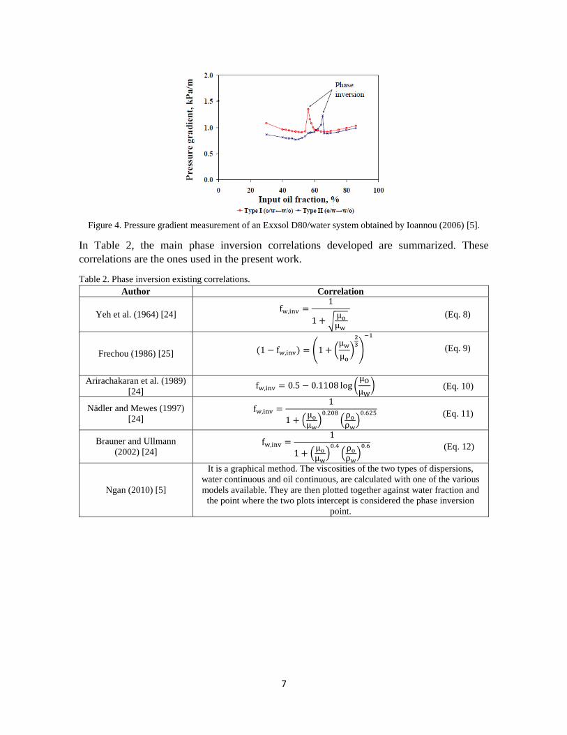
the changes are still not accurately described. An example of this can be seen in Ioannou
(2006) experimental studies; he found, using Exxsol D80 and water, that phase inversion
occurs at the peak of the pressure gradient as seen in Figure 4 [23]. Although, as already said,
this result has not always been obtained.
7
Figure 4. Pressure gradient measurement of an Exxsol D80/water system obtained by Ioannou (2006) [5].
In Table 2, the main phase inversion correlations developed are summarized. These
correlations are the ones used in the present work.
Table 2. Phase inversion existing correlations.
Author Correlation
Yeh et al. (1964) [24] fw,inv =
1
1 + √μo
μw
(Eq. 8)
Frechou (1986) [25] (1 − fw,inv) = (1 + (μw
μo
)
23
)
−1
(Eq. 9)
Arirachakaran et al. (1989)
[24] fw,inv = 0.5 − 0.1108 log (
μO
μW
) (Eq. 10)
Nädler and Mewes (1997)
[24] fw,inv =
1
1 + (μo
μw)
0.208
(ρo
ρw)
0.625 (Eq. 11)
Brauner and Ullmann
(2002) [24] fw,inv =
1
1 + (μo
μw)
0.4
(ρo
ρw)
0.6 (Eq. 12)
Ngan (2010) [5]
It is a graphical method. The viscosities of the two types of dispersions,
water continuous and oil continuous, are calculated with one of the various
models available. They are then plotted together against water fraction and
the point where the two plots intercept is considered the phase inversion
point.

8
3. Dataset
The experimental dataset used, consists of 2287 registers from 27 experimental studies of
different authors in horizontal pipes, as shown in Table 3 .These authors used different fluids,
superficial velocities, pipe lengths, diameters and materials.
Table 3. Experimental data used in the present study.
Author Data Fluids Vsw [m/s] Vso [m/s]
Wall
roughness
[m]
D [m] L [m] L/D
Abubakar
(2015)
[26]
86
Water-Mineral Oil
(Shell Tellus S2
V15)
0.02-1.35 0.02-1.35 1.00E-04 0.0306 12 392.2
Al-Yaari
(2009)
[27]
85 Water-Kerosene
(SAFRA D60) 0.1-2.78 0.1-2.79 1.00E-04 0.0254 10 393.7
Angeli
(2000)
[28]
66 Water-Kerosene
(EXXSOL D80) 0.11-2.65 0.43-2.65
1.00E-
05/7.00E-05 0.024/0.0243 9.5/9.7
395.8/
399.1
Castro
(2011)
[29]
6 Water-Oil 0.015 0.03-0.15 1.00E-07 0.026 12 461.5
Dasari
(2014)
[30]
77 Water - Lubricating
Oil 0.19-1.06 0.11-1.19 1.00E-04 0.0254 1 39.4
Elseth
(2001)
[16]
159 Water-Oil (Exxsol
D-60) 0-2.99 0-3 4.50E-05 0.0563 10.2 181.3
Kathibi
(2015)
[31]
9 Tap water- Mineral
Oil 0.02-0.7 0.01-0.9 5.00E-05 0.06 16 266.7
Kumara
(2009)
[32]
69 Water-Oil
(EXXSOL D60) 0.001-1.51 0.001-1.49 4.60E-05 0.056 15 267.9
Kurban
(1997)
[33]
75 Water-Oil
(EXXSOL D80) 0.11-2.62 0.43-2.62
1.00E-
04/4.50E-05 0.024/0.0243 9.5/9.7
395.8/
399.1
Laflin
(1976)
[34]
44 Water-N° 2 Diesel
fuel 0.2-0.9 0.5-1.09 1.00E-04 0.0381 5.7 152
Liu
(2008)
[35]
41 Water-Diesel Oil 0.028-0.514 0.05-0.63 4.50E-05 0.026 11,1 429.4
Lovick
(2004)
[36]
96 Water-Oil
(EXXSOL D140) 0.001-3 0.001-3 4.50E-05 0.038 8 210.5
Mukhaimer
(2015)
[12] [37]
22
Water/Salty water-
Kerosene (Safrasol
80)
0.005-2.384 0.005-2.384 5.00E-06 0.0225 8 355.6
Nadler
(1997)
[9]
401 Water-Mineral Oil
(Shell Ondina 17) 0.001-1.5 0-1.494 1.00E-04 0.059 48 813.6
Oglesby
(1979)
[38]
238 Water-Oil 0.07-2.71 0.19-3.19 5.00E-05 0.0411 5.7 140.9
Rodriguez
(2011)
[39]
33 Water-Oil 1-3 0.2-1 1.00E-07 0.026 12 461.5

9
Schümann
(2016)
[40]
53
Tap Eater- Oil
(Exxsol D80/Primol
352)
0.04-0.90 0.05-0.9 5.00E-06 0.1 25 250.0
Shi
(2015)
[41]
32 Water- Oil (CYL
680/CYL 1000) 0.01-1 0.06-0.57 1.00E-04 0.026 1.7 66.5
Soleimani
(1999)
[42]
101 Water-Oil
(EXXSOL D80) 0-3 0-3 4.50E-05 0.0243 9.7 399.2
Souza
(2013)
[43]
150 Water-Heavy Oil 0.02-2.99 0.02-1 1.00E-07 0.026 6.1 234.6
Tan
(2015)
[44]
29 Water-Mineral
White Oil 0.05-0.66 0.39-0.79 4.60E-05 0.05 2 40.0
Trallero
(1995)
[13]
24 Water-Oil (Crystex
Af-M) 0.01-1.82 0.01-1.59 1.00E-04 0.0501 15.5 310.2
Valencia
(2003)
[45]
42 Tap Water-Oil
(Purolube 150) 0.13-1.13 0.19-1.26 5.00E-06 0.253 4 16.0
Vielma
(2008)
[46]
90 Water-Refined
mineral Oil 0.02-1.80 0.05-1.75 1.00E-04 0.0508 21.1 415.9
Wang
(2010)
[47]
85 Water-Mineral Oil 0.01-0.8 0.01-0.39 4.60E-05 0.0254 2 78.7
Yao
(2009)
[48]
59 Water-Crude Oil 0.05-0.792 0.068-0.901 4.60E-05 0.026 4 153.8
Yusuf
(2012)
[49]
115 Water-Mineral Oil 0.15-2.56 0.14-2.27 1.00E-04 0.0254 6.5 255.9
Total 2287
Since a variety of flow patterns names are found in literature, in order to homogenize the data
and classify it in the seven flow patterns already described, the tool developed by Urbano
(2015) “The probabilistic flow pattern map generator” is used [50]. The distribution of
experimental data over different parameters is shown in Figure 5 and Table 4.

10
a.) b.)
c.)
d.)
e.) f.)
Figure 5. Data distribution. a.) Flow pattern b.) Pipe inner diameter c.) Oil viscosity d.) Oil density e.)
Interfacial Tension f.) Pipe Material.
24,4%
28,6%
3,7%
7,6%
10,7%
22,1%
3,1%
Do/w
Do/w&Dw/o
Do/w&w
Dw/o
ST
ST&MI
A
0
200
400
600
800
1000
1200
0.024 0.025 0.04 0.06 0.1 Greater
No
. o
f D
ata
Po
ints
Inner diameter [m]
0
200
400
600
800
1000
1200
0,01 0,1 0,5 2
No
. o
f D
ata
Po
ints
Oil Viscosity [Pa*s]
0
100
200
300
400
500
600
700
800
900
1000
805 831 857 883 909 935 961
No
. o
f D
ata
Po
ints
Oil Density [kg/m^3]
0
100
200
300
400
500
600
700
800
900
0,02 0,03 0,04 0,05
No
. o
f D
ata
Po
ints
Interfacial Tension [N/m]
8,3%
5,1%
20,6%
10,6%
55,4%
Glass
PVC
Stainless Steel
Carbon Steel
Acrylic
11
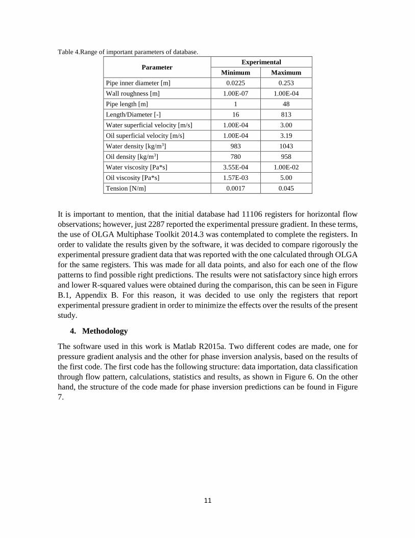
Table 4.Range of important parameters of database.
Parameter Experimental
Minimum Maximum
Pipe inner diameter [m] 0.0225 0.253
Wall roughness [m] 1.00E-07 1.00E-04
Pipe length [m] 1 48
Length/Diameter [-] 16 813
Water superficial velocity [m/s] 1.00E-04 3.00
Oil superficial velocity [m/s] 1.00E-04 3.19
Water density [kg/m3] 983 1043
Oil density [kg/m3] 780 958
Water viscosity [Pa*s] 3.55E-04 1.00E-02
Oil viscosity [Pa*s] 1.57E-03 5.00
Tension [N/m] 0.0017 0.045
It is important to mention, that the initial database had 11106 registers for horizontal flow
observations; however, just 2287 reported the experimental pressure gradient. In these terms,
the use of OLGA Multiphase Toolkit 2014.3 was contemplated to complete the registers. In
order to validate the results given by the software, it was decided to compare rigorously the
experimental pressure gradient data that was reported with the one calculated through OLGA
for the same registers. This was made for all data points, and also for each one of the flow
patterns to find possible right predictions. The results were not satisfactory since high errors
and lower R-squared values were obtained during the comparison, this can be seen in Figure
B.1, Appendix B. For this reason, it was decided to use only the registers that report
experimental pressure gradient in order to minimize the effects over the results of the present
study.
4. Methodology
The software used in this work is Matlab R2015a. Two different codes are made, one for
pressure gradient analysis and the other for phase inversion analysis, based on the results of
the first code. The first code has the following structure: data importation, data classification
through flow pattern, calculations, statistics and results, as shown in Figure 6. On the other
hand, the structure of the code made for phase inversion predictions can be found in Figure
7.

12
Figure 6. Structure of Matlab code for pressure gradient calculations.
The pressure gradient calculation part is divided by model. Each model has different inputs,
which means not all the combinations of friction correlations, mixture viscosity correlations
and pressure gradient models are evaluated. The number of combinations depend on the
model definition. As an example, the Arirachakaran correlation calculates a friction factor
for each one of the phases separately, which means no mixture viscosity correlation is used
in that case. On the other hand, for Brauner correlation, mixture viscosity correlations are
used as well as friction factor correlations, obtaining more different combinations to evaluate.
Taking this into account, all possible combinations within these limitations are evaluated.
Figure 7. Structure of Matlab code for phase inversion point predictions.
For the phase inversion point predictions, only the experimental data that report phase
inversion points for specific systems is used. This, in order to compare the phase inversion
correlations results, with the experimental phase inversion point. This part also uses the
pressure gradient results, since the relation between pressure gradient and phase inversion is
evaluated.
4.1. Statistics
Since the principal objective is to find the most practical, accurate and non-complex
correlation combination, descriptive statistic and specific model comparison criteria are used.
Here, the experimental data reported in the database and the one calculated for each pattern,
as described before, are compared and analyzed.
Data flow pattern
classification
Data import from Excel to
Matlab
ST
ST&MI
Do/w
Dw/o
Do/w & w
Do/w & Dw/o
CAF
Pressure gradient calculation: all
possible combinations
depending on the model (friction factor and mixture viscosity
correlations)
Statistical criterions
and validation
of the results
Results: graphics
and tables
Classification of data
depending on author and
mixture velocity
Data import with
calculated pressure gradient
Phase inversion
point calculation
through different
correlations
Graphic of calculated pressure
gradient data against water
cut
Graphic with predicted
phase inversion
points

13
Table 5. Statistical parameters used in the present work.
Statistical parameter Equation
Average Percent Error (%)
[51]
ei =dPdzcalc − dPdzexp
dPdzexp
(Eq. 13)
E1, % =1
n ∑ ei
n
i=1
∗ 100 (Eq. 14)
Absolute Average Percent Error (%)
[51] E2, % =
1
n ∑|ei|
n
i=1
∗ 100 (Eq. 15)
Percent Standard Deviation (%)
[51] E3, % = ∑ √(ei ∗ 100 − E1)2
n − 1
n
i=1
(Eq. 16)
Average Error (Pa/m)
[51]
eii = dPdzcalc − dPdzexp (Eq. 17)
E4 =1
n ∑ eii
n
ii=1
(Eq. 18)
Absolute Average Error (Pa/m)
[51] E5 =
1
n ∑|eii|
n
ii=1
(Eq. 19)
Standard Deviation (Pa/m)
[51] E6 = ∑ √(eii − E4)2
n − 1
n
ii=1
(Eq. 20)
Relative Performance Factor (-)
[52] FRP = ∑
|Ei| − |Ei,min|
|Ei,max| − |Ei,min|
6
i=1
(Eq. 21)
R-squared [53]
a = ∑ dPdzexp ∗ dPdzcalc
n
i=1
(Eq. 22)
b =1
n ∑ dPdzexp
n
i=1
∑ dPdzcalc
n
i=1
(Eq. 23)
c = ∑ dPdzexp2
n
i=1
−1
n(∑ dPdzexp
n
i=1
)
2
(Eq. 24)
d = ∑ dPdzcalc2
n
i=1
−1
n(∑ dPdzcalc
n
i=1
)
2
(Eq. 25)
R2 =(a − b)2
(c ∗ d) (Eq. 26)
Akaike Information Criterion [14] AIC = n ln (∑ eii2
n
i=0
) + 2K (Eq. 27)
The average percentage error (E1) and the average error (E4) indicate the agreement between
calculated and measured data. Positive values imply overprediction and negative values
underprediction. The absolute average percentage error (E2) and the absolute average error
(E5), represent the general percentage error of the calculations. The percent standard
deviation (E3) and standard deviation (E6) indicate the scatter of the error in respect to their
corresponding average error. The three first terms are based on percentage error rather than
relative pressure error, which means relative small pressure error that experience a small
pressure gradient may give a large percentage error even though the pressure error itself is

14
not that far from the actual measurements. In order to make the statistics independent of the
magnitude of pressure gradient the other three identical statistical parameters are defined [51,
52].
In addition, the relative performance factor (FRP) created by Ansari et al (1994) [52] is a
composite error factor with descriptive statistic criteria in it. The minimum and maximum
possible values of FRP are 0 and 6, corresponding to the best and worst prediction
performance. The value of R-squared is a statistical measure of how close the data are to the
real values and in general, the higher the value, the better the model fits the data. On the other
hand, the Akaike Information Criterion for a given data set has no meaning by itself, although
the value can be interpreted if it is compared with the AICs of a series of models based on
the same data set (observations) with the same dependent variables. Since this criterion takes
into account the variables used by the model, a complexity comparison is being made, the
lower the AIC most appropriate the model [54].
5. Results and analysis
In this section results are presented in order. First pressure gradient model analysis, followed
by phase inversion results.
5.1. Pressure gradient
Since each pressure gradient model was defined for a specific flow pattern, only the possible
combinations within these models are evaluated. Since statistical analysis was made to
evaluate the performance of each combination, trying to find the most practical, accurate and
non-complex model, only the five best combinations with their statistics and graphical results
are presented.
Stratified flow (ST)
For this pattern, 40 possible combinations were found to be valid for the 244 experimental
data points. The graphical and statistical results of the best five combinations are presented
in Table 6 and Figure 8.
Table 6. Statistical results for ST.
Pressure
Gradient
Model
Friction
Factor
Correlation
E1
(%)
E2
(%)
E3
(%)
E4
(Pa/m)
E5
(Pa/m)
E6
(Pa/m) FRP R2 AIC
Elseth
(2001) (Eq. 6)
Danish et al.
(2011) (Eq. 84)
-40.89 42.83 69.26 -66.53 68.15 186.89 0.011 0.64 202.20
Elseth
(2001) (Eq. 6)
Drew et al.
(1936) (Eq. 32)
-42.96 44.70 67.73 -69.13 70.59 189.99 0.013 0.67 202.90
Arirachakaran
(1989)
(Eq. 1)
Churchill
(1977)
(Eq. 43)
-9.35 64.09 931.55 -1043.89 1807.90 39244.85 2.86 E-07
0.16 5563.17
Arirachakaran
(1989)
(Eq. 1)
Morrison (2013)
(Eq. 90)
-10.62 64.60 930.30 -1044.34 1808.20 39243.28 3.01 E-07
0.16 5563.17
Arirachakaran (1989)
(Eq. 1)
Wood (1966)
(Eq. 37)
-64.28 67.30 362.45 -2036.54 2044.74 49070.68 7.88
E-07 0.20 5610.93

15
Based on the statistical parameters results, there is a tendency to underestimate the pressure
gradient value in all combinations. As it can be seen, the average error is between 42 and
45% for combinations using Elseth (2001) model and between 64 and 69% for models using
the Arirachakaran (1989) model. The main difference between these two models is that the
first one takes into account the interfacial shear stress between the phases, while the second
one is a correlation that calculates pressure gradient for each phase separately. The statistic
parameters are better for the first two combinations. The standard deviation is lower and the
R-squared showed a better response of the data. The relative performance factor (FRP) and
the AIC, agreed that the two first combinations are much better than the other ones in terms
of parameters and basic statistics.
a.) b.)
c.) d.)
e.)
Figure 8. Graphical results for the best combinations in ST within ±40% error. a.) Elseth and Danish et al.
b.) Elseth and Drew et al. c.) Arirachakaran and Churchill d.) Arirachakaran and Morrison e.) Arirachakaran
and Wood.

16
The graphical results presented, confirm the underestimation of the pressure gradient in all
cases agreeing to the statistical results presented. In addition, a very similar behavior between
the two first options can be seen. The two friction factor correlations were developed for
either turbulent or laminar regime, although the one developed by Drew et al. (1936) is not
an explicit equation as the one developed by Danish et al. (2011). This made the use of the
first correlation slightly more complicated than the second one. It is important to mention,
that this pattern is not characterized by a higher-pressure gradient, which affects the
calculation of a few combinations due to the fact, that some friction factor correlations were
developed specifically for turbulent flow, i.e. higher Reynolds numbers. In addition, this
pattern was defined as with a smooth interface which agreed with the assumptions made by
the Elseth (2011) model. The error encountered for the first combination, is still significant,
but it represents a good first approach to the calculation of pressure gradient for stratified
flow regimes.
Stratified flow with mixture at the interface (ST&MI)
For this pattern 505 experimental data points, 44 possible combinations were evaluated using
the two models for stratified flow. The summary of the results of the best five combinations
can be seen in Table 7 and Figure 9.
Table 7.Statistical results for ST&MI.
Pressure
Gradient
Model
Friction
Factor
Correlation
E1
(%)
E2
(%)
E3
(%)
E4
(Pa/m)
E5
(Pa/m)
E6
(Pa/m)
FRP
*10-4 R2 AIC
Elseth (2001)
(Eq. 6)
Drew et al. (1936)
(Eq. 32)
-2.88 57.29 1279.57 -2209.68 2330.42 80459.71 5.85 0.10 11980.34
Arirachakaran
(1989) (Eq. 1)
Brkic b
(2011) (Eq. 83)
-59.53 65.16 555.50 -2357.88 2405.77 80236.09 6.92 0.05 11990.03
Arirachakaran
(1989) (Eq. 1)
Brkic a
(2011) (Eq. 81)
-61.30 66.06 530.60 -2372.44 2413.58 80406.89 7.00 0.05 11991.65
Arirachakaran
(1989)
(Eq. 1)
Avci &
Karagoz
(2009)
(Eq. 79)
-59.61 66.54 568.51 -2348.48 2421.15 80332.14 6.96 0.03 11994.55
Arirachakaran (1989)
(Eq. 1)
Wood (1966)
(Eq. 37)
-58.84 67.64 603.91 -2336.62 2403.74 79512.84 6.86 0.07 11982.31
In this case, the average error according to the results lies between 57 and 68%. The pressure
gradient values are being underpredicted in all combinations. It is found that the best
combination uses Elseth (2001) model, based on momentum balance equations, while the
other four use the Arirachakaran (1989) model. The characteristic of this pattern, which can
have a possible mixing at the interface complicates the calculation taking into account that
both models assumed a smooth flat interface and take it as a straight line for the geometry
parameters needed. Although the first model gives a lower value of average error, it gives a
very high standard deviation which can significantly affect the pressure gradient results.

17
However, this combination is classified by the FRP, R-squared and the AIC as the best one
in terms of parameters and precision.
All the friction factor correlations obtained for the Arirachakaran (1989) combinations are
explicit simple equations, which make them none so complex to use. However, the Drew et
al. (1936) correlation combined with the Elseth (2001) model gives better results. This
correlation is not explicit but with the pressure gradient model used, is found to be the best
one in terms of parameters.
a.) b.)
c.) d.)
e.)
Figure 9. Graphical results for the best combinations in ST&MI within ±50% error. a.) Elseth and Drew et al.
b.) Arirachakaran and Brkic b c.) Arirachakaran and Brkic a d.) Arirachakaran and Avci & Karagoz e.)
Arirachakaran and Wood.

18
The graphical results presented, confirm the underestimation of the pressure gradient in all
cases agreeing to the statistical results presented, but the first combination shows a lower
tendency to underestimate the value compared to the others. This pattern is characterized by
lower pressure gradient values but already higher than those for stratified flow regime. It is
clearly seen, that the mixing at the interface which is not being taken into account in the
models affects the results. As a first approach a good result is obtained, however the
evaluation of dispersed flow models combined with stratified ones could be a reasonable next
step.
Dispersion of oil in water and water (Do/w & w)
In this case, for the 84 experimental data points 777 combinations were found to be valid for
this pattern; the five best combinations according to statistical parameters are summarized in
Table 8 and Figure 10.
Table 8.Statistical results for Do/w & w.
Pressure
Gradient
Model
Mixture
Viscosity
Correlation
Friction
Factor
Correlation
E1
(%)
E2
(%)
E3
(%)
E4
(Pa/m)
E5
(Pa/m)
E6
(Pa/m)
FRP
*10-5 R2 AIC
Brauner (2002)
(Eq. 3)
Taylor (1932)
(Eq. 94)
Drew &
Generaux
(1936) (Eq. 32)
-5.27 25.38 234.06 -256.97 323.83 4197.93 2.09 0.024 1506.66
Brauner
(2002)
(Eq. 3)
Barnea &
Mizrahi (1975)
(Eq. 110)
Drew &
Generaux (1936)
(Eq. 37)
-6.66 25.38 231.64 -260.73 324.88 4195.63 2.16 0.024 1506.86
Brauner
(2002)
(Eq. 3)
Einstein
(1906)
(Eq. 93)
Drew &
Generaux (1936)
(Eq. 37)
-4.80 25.50 235.70 -255.60 324.19 4200.95 2.08 0.024 1506.65
Brauner
(2002) (Eq. 3)
Yaron & Gal-Or
(1972)
(Eq. 107)
Drew & Generaux
(1936)
(Eq. 37)
-4.37 25.60 237.56 -255.14 325.07 4208.29 2.07 0.024 1506.79
Brauner
(2002) (Eq. 3)
Pal 1
(2001) (Eq. 114)
Drew & Generaux
(1936)
(Eq. 37)
-4.38 25.71 237.16 -252.64 324.12 4197.36 2.06 0.023 1506.48
Based on the statistical results, the best five combinations obtain a very good result with an
average error between 25 and 26%. It can be seen that all the combinations tend to
underestimate the pressure gradient; although, all have the same R-squared and a similar
value for the AIC and FRP criterions.
For all combinations, the Brauner (2002) model developed for dispersed flow is the best
option in this case; this taking the oil as the dispersed phase in water. In the case of the friction
factor correlations, the Drew & Generaux (1936) one is found to be the best one among all
the other ones. This correlation is an implicit and simple equation for the calculation of the
friction factor, and it happens to be very similar to the ones proposed by Prandtl (1935) and
Colebrook (1939), which are commonly used. In the case of the mixture viscosity calculation,
simple equations as the ones by Taylor (1932) and Einstein (1906) are found in the best five

19
combinations. Even if the other ones tend to be slightly more complex to solve they also
show a good result combining them with the pressure gradient model and respective friction
factor correlation.
a.) b.)
c.) d.)
e.)
Figure 10. Graphical results for the best combinations in Do/w & w within ±25% error. a.) Brauner, Taylor
and Drew et al. b.) Brauner, Barnea et al. and Drew et al. c.) Brauner, Einstein and Drew et al. d.) Brauner,
Yaron et al. and Drew et al. e.) Brauner, Pal and Drew et al.
In the graphical results, is clearly seen that for lower pressure gradient values the fit of the
combination of model and correlations is better. The five combinations evaluated, tend to
have the same prediction with some points with high values of pressure gradient, which could
be a mistake during data classification. Is interesting how this pattern can be modeled as an

20
oil in water dispersion, since no specific model has being developed for it and it is not a total
dispersion one phase in the continuum of the other. However, the fact that is a dispersion is
being reflected in the calculation of mixture properties, which takes into account the mixture
of the continuous and dispersed phase, but also the volume fraction of the dispersed phase.
A really good approach of the values is obtained, but it is also important, to note that this is
the dispersed flow pattern with less number of data points, which affect the statistical results.
Dispersion of oil in water (Do/w)
For this pattern, the total number of valid combinations was of 765 for the 557 experimental
data points. The results of the best five combinations according to statistic criteria are
presented in Table 9 and Figure 11.
Table 9.Statistical results for Do/w.
Pressure
Gradient
Model
Mixture
Viscosity
Correlation
Friction
Factor
Correlation
E1
(%)
E2
(%)
E3
(%)
E4
(Pa/m)
E5
(Pa/m)
E6
(Pa/m)
FRP
*10-9 R2 AIC
Brauner
(2002) (Eq. 3)
Eiler
(1962) (Eq. 103)
Danish et al
(2011) (Eq. 84)
4.97 27.29 656.78 -117.61 618.62 15126.10 5.31 0.65 11209.42
Brauner
(2002)
(Eq. 3)
Taylor
(1932)
(Eq. 94)
Danish et al
(2011)
(Eq. 84)
3.94 27.94 673.58 -131.44 633.60 15419.61 5.67 0.64 11233.60
Brauner
(2002)
(Eq. 3)
Einstein
(1906)
(Eq. 93)
Danish et al
(2011)
(Eq. 84)
5.44 28.69 692.79 -93.19 646.10 15582.00 6.31 0.63 11248.15
Brauner
(2002) (Eq. 3)
Dougherty & Krieger
(1959)
(Eq. 102)
Drew & Generaux
(1936)
(Eq. 37)
-13.29 28.77 613.27 -576.39 763.63 18298.74 1.53 0.60 11420.85
Brauner
(2002)
(Eq. 3)
Pal 1
(2001)
(Eq. 114)
Danish et al
(2011)
(Eq. 84)
8.32 30.15 733.68 -31.96 661.02 15705.09 7.57 0.63 11264.76
Based on the statistical parameters results the best five combinations of correlations have average
errors lower than 30%. Fourth combinations out of five, tend to overestimate the pressure
gradient similarly. In general, a similar standard deviation, FRP values, R-squared and AIC
values are encountered.
According to the results, there is no doubt that the best pressure gradient model for this pattern
is the one proposed by Brauner (2002), which was specially developed for this pattern and was
applied using oil as the dispersed phase and water as the continuous phase. For the friction factor
correlation, is Danish et al. (2011) explicit equation the best in four cases. This result is consistent
with the fact that as this correlation was proposed it was found that it works for all practical
ranges, in laminar and turbulent flow [55], this is not a characteristic of all the friction factor
correlations studied. On the other hand, the implicit correlation from Drew et al. (1936) appears
again within the best results. In terms of mixture viscosity correlations, the ones obtained to be
the best in this case, are characterized by their simplicity in calculation; again, Taylor (1962),
Eiler (1962) and Einstein (1906), correlations obtained the best results calculating this mixture
property.

21
a.) b.)
c.) d.)
e.)
Figure 11. Graphical results for the best combinations in Do/w within ±25% error. a.) Brauner, Eiler and
Danish et al. b.) Brauner, Taylor and Danish et al. c.) Brauner, Einstein and Danish et al. d.) Brauner,
Dougherty & Krieger and Drew et al. e.) Brauner, Pal and Danish et al.
As it can be seen in the graphical results, the fourth combination has a tendency to
underestimate the value, which agrees with the statistical result. However, in the other four
cases the overprediction is not evident since this pattern has a significant amount of data
points. The results were expected since the Brauner (2002) model was specially developed
for this pattern and mixture viscosity correlations can be clearly defined with oil as the
dispersed phase and water as the continuous one.

22
Dispersion of water in oil (Dw/o)
In the case of this pattern, for the 173 experimental data points, 774 possible combinations
were encountered. The statistical and graphical results of the best five combinations are
presented in Table 10 and Figure 12.
Table 10.Statistical results for Dw/o.
Pressure
Gradient
Model
Mixture
Viscosity
Correlation
Friction
Factor
Correlation
E1
(%)
E2
(%)
E3
(%)
E4
(Pa/m)
E5
(Pa/m)
E6
(Pa/m)
FRP
*10-5 R2 AIC
Brauner
(2002)
(Eq. 3)
Dougherty &
Krieger (1959)
(Eq. 102)
Danish et al.
(2011)
(Eq. 84)
29.18 46.23 667.37 -83.27 951.69 12913.46 0.10 0.11 3631.67
Brauner
(2002) (Eq. 3)
Barnea & Mizrahi
(1975)
(Eq. 110)
Danish et al.
(2011) (Eq. 84)
34.93 50.37 741.47 58.07 1004.81 13216.68 0.53 0.11 3635.96
Brauner (2002)
(Eq. 3)
Dougherty &
Krieger
(1959) (Eq. 102)
Drew &
Generaux
(1936) (Eq. 32)
43.73 54.08 701.55 180.01 1022.87 12965.33 1.30 0.10 3638.83
Brauner (2002)
(Eq. 3)
Barnea &
Mizrahi
(1975) (Eq. 110)
Drew &
Generaux
(1936) (Eq. 32)
49.45 59.04 776.95 321.47 112.21 14056.60 2.70 0.10 3646.52
Brauner
(2002) (Eq. 3)
Taylor
(1932) (Eq. 94)
Danish et al.
(2011) (Eq. 84)
50.26 60.64 858.52 296.30 1099.22 14356.68 2.72 0.11 3641.69
Taking into account the statistical results presented, almost the same mixture viscosity and
friction factor correlations as in the previous pattern are found. However, the statistical results
are different, obtaining an error between 56 and 61%. On one hand, the five combinations
showed a similar deviation and a tendency to overestimate the value. On the other hand, the
R-squared does not really vary between the options. In terms of the AIC criterion and the
FRP, the best combination is found to be the first one.

23
a.) b.)
c.) d.)
e.)
Figure 12. Graphical results for the best combinations in Dw/o within ±40% error. a.) Brauner, Dougherty et
al and Danish et al. b.) Brauner, Barnea et al and Danish et al. c.) Brauner, Dougherty et al. and Drew et al.
d.) Brauner, Barnea et al and Drew et al. e.) Brauner, Taylor and Danish et al.
The graphical results reflect the statistical results discussed, the overestimation and error. It
is interesting how almost the same combinations were encountered for the two dispersion
patterns; however, the results are clearly better when the dispersed phase is water and not the
oil. This could be attributed to the mixture viscosity correlations, which in this case work
better when the continuous phase has a lower viscosity than the dispersed one. The prediction
of pressure gradient for this pattern is not as expected, but it is the best approach until now.

24
For the reason of phase inversion, this pressure gradient model should be studied and
improved.
Dispersion of water in oil and oil in water (Dw/o & Do/w)
In this case, 669 combinations were found possible for the 653 experimental data points of
this pattern. The best five combinations are presented in Table 11and Figure 13.
Table 11.Statistical results for Do/w & Dw/o.
Pressure
Gradient
Model
Mixture
Viscosity
Correlation
Friction
Factor
Correlation
E1
(%)
E2
(%)
E3
(%)
E4
(Pa/m)
E5
(Pa/m)
E6
(Pa/m)
FRP
*10-8 R2 AIC
Brauner
(2002) (Eq. 3)
Dougherty & Krieger
(1959)
(Eq. 102)
Danish et al
(2011) (Eq. 84)
5.82 48.43 1264.17 -503.87 937.74 28919.17 0.48 0.03 14693.82
Brauner (2002)
(Eq. 3)
Dougherty &
Krieger
(1959) (Eq. 102)
Drew &
Generaux
(1936) (Eq. 32)
18.04 51.97 1359.26 -404.11 946.45 29003.22 0.58 0.02 14696.20
Brauner (2002)
(Eq. 3)
Barnea &
Mizrahi
(1975) (Eq. 110)
Danish et al (2011)
(Eq. 84)
66.17 90.64 2423.14 71.14 1240.14 31369.05 1.81 0.01 14761.52
Brauner
(2002)
(Eq. 3)
Barnea &
Mizrahi (1975)
(Eq. 110)
Drew &
Generaux (1936)
(Eq. 32)
73.12 95.06 2353.74 108.22 1251.10 31120.66 1.97 0.01 14752.50
Brauner
(2002) (Eq. 3)
Taylor
(1932) (Eq. 94)
Danish et al
(2011) (Eq. 84)
74.74 95.46 2457.39 170.33 1279.98 31859.02 2.14 0.02 14755.82
Since this pattern does not really have a specific model for itself, but it is clear that it is a
dispersion, the Brauner (2002) model was evaluated. In this case, the best five combinations
were encountered using the model with the dispersed phase as water and the continuous one
as oil. The average error for the two best combinations is between 48 and 52%; while the
other combinations have a significant error above 90%. According to the results, there is a
tendency to overpredict the values. A really high standard deviation value is found, however,
the first and the second combinations are really similar according to the FRP, R-squared and
AIC values. Again, the two friction correlations found to be the best ones, are the ones
developed by Danish et al. (2011) and Drew & Generaux (1936).

25
a.) b.)
c.) d.)
e.)
Figure 13. Graphical results for the best combinations in Do/w & Dw/o within ±45% error. a.) Brauner,
Dougherty et al. and Danish et al. b.) Brauner, Dougherty et al. and Drew et al. c.) Brauner, Barnea et al. and
Danish et al. d.) Brauner, Barnea et al. and Drew et al. e.) Brauner, Taylor and Danish et al.
In the plots, the overestimation can be easily identified. It is interesting how the best result is
found as a dispersion of water in oil, however, this pattern need a model for itself since it is
not entirely true that the regime is oil dominant. The results obtained are a good first
approach, but a better model or way to include both dispersions in the calculations is needed.
Core-annular flow (CAF)
For this pattern, 38 possible combinations were evaluated for the 71 experimental data points.
The statistical and graphical results of the five best combinations can be found in Table 12
and Figure 14.

26
Table 12.Statistical results for CAF.
Pressure
Gradient
Model
Mixture
Viscosity
Correlation
Friction Factor
Correlation
E1
(%)
E2
(%)
E3
(%)
E4
(Pa/m)
E5
(Pa/m)
E6
(Pa/m)
FRP
*10-8
R2
*10-3 AIC
Brauner CAF
(2002) (Eq. 4)
-
Morrison
(2013) (Eq. 90)
25.94 71.33 580.37 -1076.39 2340.00 23239.33 0.96 4.48 1540.83
Brauner CAF
(2002) (Eq. 4)
-
Blausius
(1913) (Eq. 29)
26.29 74.72 597.30 -1065.52 2403.25 24212.35 1.06 2.84 1541.37
Brauner CAF (2002)
(Eq. 4)
-
Hagen &
Poiseuille
(1840)
(Eq. 28)
-76.11 76.11 107.98 -2677.84 2677.84 20294.91 2.26 1.34 1545.25
Brauner CAF
(2002) (Eq. 4)
-
Wood
(1966) (Eq. 37)
30.74 78.07 654.83 -1091.99 2325.55 23510.65 1.03 3.18 1540.27
Brauner CAF
(2002)
(Eq. 4)
-
Brkic a
(2011)
(Eq. 81)
35.15 82.16 673.32 -1009.87 2412.27 24042.41 1.10 3.39 1540.91
It is evident, that the amount of data for this pattern is significantly lower as for the other
patterns, the average error of the evaluated combinations was between 70 and 90%. This
results were obtained taking the oil phase as the core and the water phase as the annulus,
which is the most common result due to viscosities.
Four out of the five combinations overestimate the pressure gradient value, while the others
underestimate it. However, the third one obtained the lowest standard deviation. The R-
squared is really low for all the combinations which shows that it does not really fit the data.
Even though, the FRP and AIC criterion show a similar result for all combinations. The
friction factor correlations obtained are simple explicit equations, such as the one by Wood,
Blausius and Hagen & Poiseuille, which were almost the first approaches for the prediction
of the friction factors.

27
a.) b.)
c.) d.)
e.)
Figure 14. Graphical results for the best combinations in CAF within ±70% error. a.) Brauner CAF and
Morrison. b.) Brauner CAF and Blausius. c.) Brauner CAF and Hagen & Poiseuille. d.) Brauner CAF and
Wood. e.) Brauner CAF and Brkic a.
The graphical results agree to the statistical results already discussed. The underestimation
of the value by the third combination is evident. It is important to mention, that the
probabilistic tool used to classify the data does not have this pattern include; therefore, the
classification was made taking into account the pattern reported by the authors which can
affect the results encountered. It is necessary to extend the database for this pattern in order
to make a stronger analysis.

28
5.2. Phase Inversion
For this analysis, just the data of a few authors was used. The data was chosen, according to
viscosities, densities, number of data points and wide range of mixture viscosity data. All this
in order, to analyze how the phase inversion prediction changes, depending on fluid
properties and mixture velocities. The other determining criteria, was that the author reported
the experimental value or range of phase inversion obtained during their experiments.
All the correlations, showed in Table 2 were used. In the case of the last method, the one
proposed by Ngan (2010), the 21 mixture viscosity correlations listed on Table A.1.2 in
Appendix A, were evaluated, and just the five best results among them are showed with the
other five first correlations results. In the following sections, the results for the data of each
author is presented.
5.2.1. Al-Yaari (2009)
For this experimental set up, the author used water, with a density of 998 kg/m3 and a
viscosity of 0.001 Pa*s, and Kerosene (Safra D60) with a density of 780 kg/m3 and a viscosity
of 0.0015 Pa*s [27].
Figure 15. Predicted phase inversion points with each correlation for Al-Yaari (2009) data. The lines represent
the experimental range for phase inversion reported by the author.
According to the results obtained, just two of the models obtained a phase inversion point in
the experimental range reported. The other ones, tend to overestimate the point. It is
interesting how simple mixture viscosity models, as the ones by Taylor (1932) and Einstein
(1906), are in this case the best models predicting the phase inversion point. It is also evident,
that the method proposed by Ngan (2010), used with the five best chosen correlations in this
case, give better results than the other literature correlations, as concluded by Ngan (2010)
[5]. The third best result was obtained using the Pal (2001) correlation, which according to
Ngan (2010) [5] it usually obtains a really close value to the range for oils around this
viscosity.

29
Figure 16. Calculated pressure gradient for different mixture velocities for Al-Yaari (2009) data. The lines
represent the experimental range for phase inversion reported by the author.
Since the study of the relation between pressure gradient and phase inversion is also of
interest, the results of calculated pressure gradient versus water fraction were also plotted.
As it can be seen, pressure is higher with higher mixture velocity, as expected. However,
there is a different point for each of them, for the reason of the different degree of mixing for
each mixture velocity [27], where a significant change on pressure gradient can be seen. For
lower mixture velocities, this point tends to be at higher values of water fraction, as it can be
seen for the mixture velocities 1.5 and 2 m/s. This result does not really agree with the
experimental data obtained by Al-Yaari (2009) [27], because the change of pressure gradient
for this velocities, where the pattern is usually stratified or stratified with mixing at the
interface, is not from that magnitude. However, for the highest velocities, 3 and 3.5 m/s, the
greatest change of pressure gradient measurement occur at a water fraction of 0.3
approximately. According to Al-Yaari (2009) [27], the phase inversion is assumed to happen
at or after a peak of the pressure, which in this case does not exist, since pressure gradient
increases until almost a water fraction of 0.6. For the mixture viscosities studied in this case,
a clear relation between calculated pressure gradient and phase inversion cannot be
established.
5.2.2. Elseth (2001)
In this case, the experimental data was obtained using water with density of 1000 kg/m3 and
viscosity of 0.001 Pa*s, and oil (Exxsol D-60), with a density of 790 kg/m3 and a viscosity
of 0.016 Pa*s [16]. Very similar properties with the fluids used by Al-Yaari (2009).

30
Figure 17. Predicted phase inversion points with each correlation for Elseth (2001) data. The lines represent
the experimental range for phase inversion reported by the author.
In this case, the best five mixture viscosities correlations found to be the best ones for the
prediction of phase inversion point through Ngan (2010) method, are again the ones obtained
before for Al-Yaari (2009). The simplest ones, from Taylor (1932) and Einstein (1906),
obtain again a predicted value within the experimental range and the other three close values.
The literature correlations, overestimate again the phase inversion point and obtain close
values to the upper limit of the experimental range reported.
Figure 18. Calculated pressure gradient for different mixture velocities for Elseth (2001) data. The lines
represent the experimental range for phase inversion reported by the author.
As showed, in Figure 18, the pressure gradient increases as mixture velocity increases. For
the velocities lower than 1 m/s there is not a specific peak of pressure that can be identified.
Although, an increase of pressure is found at high water fractions. For velocities higher than
1 m/s the author reported a water fraction of 0.27 for phase inversion. As it can be seen, for
velocities 1.34, 1.5 and 2 m/s, the peak of pressure gradient is found in a higher water fraction,
which agrees some results of calculated points through correlations. While for 2.5 and 2.67
m/s the peak is found within the experimental range reported and very close to two best
results of correlations. According to these results, it can be concluded that for intermediate

31
mixture velocities, the pressure gradient calculation tend to be more accurate and tend to
meet the predictions of phase inversion points better. Also, a relation described by Abubakar
(2015) [26] is also seen, which affirms that as mixture velocity increases the phase inversion
point decreases.
5.2.3. Nadler (1997)
This author did his experiments using water and mineral white oil (Shell Ondina 17) varying
the temperature of the experiments between 18 and 30°C, obtaining different fluid properties,
showed and classified as follows:
Low viscosity oil: density 846.26 kg/m3 and viscosity 0.022 Pa*s. Water: density 995.6
kg/m3 and viscosity 0.00078 Pa*s.
Figure 19. Predicted phase inversion points with each correlation for Nadler (1997) low viscosity oil data. The
lines represent the experimental range for phase inversion reported by the author.
In this case, only four of the predicted points fall out of the experimental range, which tend
to slightly overestimate the point. However, really good results were obtained with mixture
viscosities correlations and in the case of literature correlations, with the one proposed by
Yeh et al. (1964) and Frechou (1986). It is important to mention, then even though this is the
low viscosity oil used in Nadler (1977) experiments, this oil has already a higher viscosity
comparing it with all the other studies taken into account; which can be reflected in the way
that different mixture viscosity correlations are obtained. The previously obtained
correlations, are now replaced by slightly more complex and complete correlations as the
ones by Vand (1948), Brinkman & Roscoe (1952), Furuse (1972) and Phan Thien & Pham
(1997).

32
Figure 20. Calculated pressure gradient for different mixture velocities for Nadler (1997) low viscosity oil
data. The lines represent the experimental range for phase inversion reported by the author.
According to the pressure gradient versus water fraction plot showed, for the mixture velocity
of 1.5 m/s, there is no peak of pressure gradient within the experimental range, however, a
fall in the pressure gradient is presented as the water fraction increases. In the case of 0.3 and
0.6 m/s velocities, a peak in pressure can be seen when the water fraction is too low and also
when it is too high. In the case of the 0.9 m/s velocity, the peak of pressure gradient is also
seen for very low water fractions. These results do not agree with the experimental range of
phase inversion identified by the author. In this case, almost for all mixture velocities a
stratified pattern is encountered, which make the prediction of pressure gradient difficult and
it can be reflected since peaks of pressure gradient calculations should be related to the phase
inversion point of dispersed patterns.
Medium viscosity oil: density 847.45 kg/m3 and viscosity 0.0267 Pa*s. Water: density
997 kg/m3 and viscosity 0.00089 Pa*s.
Figure 21. Predicted phase inversion points with each correlation for Nadler (1997) medium viscosity oil data.
The lines represent the experimental range for phase inversion reported by the author.

33
For this oil properties, all the ten predictions obtained a very good result. However, the same
three literature correlations, by Arirachakaran et al. (1989), Nädler and Mewes (1997) and
Brauner und Ullman (2002) do overestimate the value, while the one by Frechou (1986) tends
to underestimate it. In addition, again the same mixture viscosity correlations obtained for
the low viscosity oil of this study, are obtained with a good prediction within the experimental
range.
Figure 22. Calculated pressure gradient for different mixture velocities for Nadler (1997) medium viscosity
oil data. The lines represent the experimental range for phase inversion reported by the author.
Since oil viscosity increases, it is expected that the calculated pressure gradient increases too.
This result is obtained; however the peak of pressure gradient for high mixture viscosity is
again near high water fractions. In the case of the lowest velocities, 0.3 and 0.6 m/s, a peak
of pressure gradient is found also towards highest water fractions. The pressure gradient
results, do not meet the phase inversion predictions nor experimental values.
High viscosity oil: density 848.81 kg/m3 and viscosity 0.035 Pa*s. Water: density 998.6
kg/m3 and viscosity 0.001 Pa*s.
Figure 23. Predicted phase inversion points with each correlation for Nadler (1997) high viscosity oil data.
The lines represent the experimental range reported by the author.

34
For the high viscosity oil of this data, the same result in terms of literature correlations and
mixture viscosity correlations was encountered. However, it can be seen that as oil viscosity
increases the predictions by the mixture viscosity correlations, the Yeh et al. (1964) and
Frechou (1966) correlations, are moved slightly to the left, to lower water fractions.
According to this result, as the viscosity increases the predicted phase inversion point
decreases.
Figure 24. Calculated pressure gradient for different mixture velocities for Nadler (1997) high viscosity oil
data. The lines represent the experimental range reported by the author.
In this case, the pressure gradient values do not show a clear relation with phase inversion
ones. However, the calculated pressure gradients values do increase with the increase of the
oil viscosity.
5.2.4. Soleimani (1999)
In this case for the experiments, water with a density of 997 kg/m3 and a viscosity of 0.001
Pa*s and an oil (Exxsol D80), with density of 801 kg/m3 and a viscosity of 0.0016 Pa*s were
used [42].
Figure 25. Predicted phase inversion points with each correlation for Soleimani (1999) data. The lines
represent the experimental range reported by the author.
For this case, all the best ten correlations predict a really close value of phase inversion point.
In the case of mixture viscosity correlations, the correlation of Guth & Simha (1936),

35
Vermuelen et al. (1955) and Pal (2001) appear again. In this case the correlation that best
predict the point is the one developed by Pal (2001). The mixture viscosity method tends to
have better results than the other literature correlations, however, as said before, the results
are very close. The phase inversion experimental range reported is between 0.3 and 0.4, and
almost all the models, overestimate the point near to the upper limit of the range.
Figure 26. Calculated pressure gradient for different mixture velocities for Soleimani (1999) data. The lines
represent the experimental range reported by the author.
In this case the data was taken experimentally for three different mixture velocities. For this
study the oil properties, are very similar to the ones for the oil in the case of Al-Yaari (2009)
and Elseth (2001). Again, the intermediate mixture velocity does have a peak of pressure
gradient within the experimental range while the other ones, in the case of the lowest mixture
velocity tend to be for a higher water fraction and in the case of the highest mixture velocity
for a lower water fraction. The peak for the velocity of 2.5 m/s is the one closest to the
correlations predictions. Again, a relation between pressure gradient and phase inversion is
seen just for intermediate velocities. The fact that phase inversion point decreases as mixture
velocity increases can be seen in this case too.
6. Conclusions and future work
Pressure gradient
A statistical and physical analysis was made for each combination possible of: pressure
gradient models, mixture viscosity correlations and friction factor models. As a result, the
best combination for calculating pressure gradient for liquid-liquid flow in each pattern is:
For ST: Elseth model and Danish et al. friction factor correlation with an average
error of 42.8%.
For ST&MI: Elseth model and Drew et al. friction factor correlation with an average
error of 57.2%.
For Do/w & w: Brauner model, Taylor mixture viscosity correlation and Drew et al.
friction factor correlation with an average error of 25.3%.
For Do/w: Brauner model, Eiler mixture viscosity correlation and Danish et al.
friction factor correlation with an average error of 27.2%.

36
For Dw/o: Brauner model, Dougherty & Krieger mixture viscosity correlation and
Danish et al. friction factor correlation with an average error of 46.2%.
For Do/w & Dw/o: Brauner model, Dougherty & Krieger mixture viscosity
correlation and Danish et al. friction factor correlation with an average error of
48.4%.
For CAF: Brauner CAF model and Morrison friction factor correlation with an
average error of 71.3%.
It is important to mention, that the combinations were chosen based on the results presented
previously; these correlations are the ones with less average error, variability and according
to the AIC criterion of less complexity, in terms of parameters, in comparison with the other
ones. The codes developed in Matlab R2015a, along with the statistical criterions used, were
essential in this analysis; the calculation of pressure gradient through so many possible
combinations requires a specialized software and an adequate way of classifying the results.
The Elseth (2001) model for stratified flow, appears to be the best one since it takes into
account the interfacial properties; however, for the stratified flow with mixing at the
interface, a better model that takes into account the possible entrainment of drops at one or
both side of the interface could be developed. The Brauner (2002) dispersed flow model work
better for dispersion of oil in water than for dispersions of water in oil; this model was also
used for the dispersion of oil in water and water, obtaining very good statistical results. There
is also a lack of models to calculate pressure gradient when two type of dispersions coexist.
The results obtained using the model for core annular flow were not the best, but an analysis
with more data and with a better classification could be made.
Even if the best model for each pattern was identified, to obtain more precise results, the
database could be extended. This taking into account, that all data must be experimental data
reporting pressure gradients. Also, the use of high viscosity oils in the experiments, will be
recommended, since this analysis would be nearer to the reality in the industry, where higher
viscosity oils are used. In this terms, the analysis that was made just for horizontal pipes,
should also be extended to inclined pipes. For the reason that in the industry oil-water flow
transport pipes often have an inclination different from 0 or 90 (vertical pipes) degree [16].
The next logical step for this study, could be making a fitting of the best combinations of
models for each pattern with the experimental data, in order to obtain one new simpler model
for the practice. Moreover, separating data in real oils and synthetic oils, could also be
interesting since all of the pressure gradient models evaluated, assume perfect drops; a better
response of the models will be expected for the synthetic ones.
Phase inversion
The prediction of phase inversion point was evaluated through 26 different correlations. Five
of them, were literature correlations and the others, were mixture viscosity correlations used
to calculate the phase inversion point through the method of Ngan (2010).

37
From the results, for oils with approximate viscosity of 0.01 Pa*s, as the ones used by Al-
Yaari (2009), Elseth (2011) and Soleimani (1999), a good prediction of phase inversion point
was encountered using Ngan (2010) mixture viscosity method, with correlations as simple as
the ones by Taylor and Einstein or with more appropriate ones such as the one developed by
Pal (2001). In addition, a relation between pressure gradient calculations and phase inversion
point, was only found for intermediate velocities between 2 and 3 m/s for this kind of oils.
In the case of higher oil viscosities, such as the ones used by Nadler (1997), between 0.02
and 0.04 Pa*s, the phase inversion point predictions were more accurate. The best literature
correlation was found to be the one by Yeh et al. (1946) and the mixture viscosity correlations
developed by Vand (1948), Brinkman & Roscoe (1952), Furuse (1972) and Phan Thien &
Pham (1997). The relation between pressure gradient values and phase inversion was not
clearly identified. Even though the pressure gradient value increases as oil viscosity
increases, the peaks of pressure gradient calculations are not found within the experimental
range of phase inversion reported.
According to the results, the correlations and methods used for the phase inversion point
predictions worked better for intermediate mixture velocities. A tendency of overestimating
the value for viscosity oils of 0.01 Pa*s was observed and also a tendency to underestimate
the values for higher viscosity oils. A better relation between pressure gradient and phase
inversion could be obtained if the database has more experimental data with higher mixture
viscosities and a wide range of oil viscosities, since phase inversion phenomena can be better
identified through pressure gradient under this conditions where dispersion patterns are
found.

38
7. References
[1] S. Atmaca, C. Sarica, H.-Q. Zhang and A. S. Al-Sarkhi, "Characterization of Oil/Water
Flows in Inclined Pipes," SPE Projects Facilities & Construction, vol. 4, no. 02, pp.
41-46, 2009.
[2] K. Park, M. Chinaud and P. Angeli, "Transition form stratified to non-stratified oil-
water flows using a bluff body," Experimental Thermal and Fluid Science, vol. 76, pp.
175-184, 2016.
[3] A. S. Izwan Ismail, I. Ismail, M. Zoveidavianpoor, R. Mohsin, A. Piroozian, M. S.
Misnan and M. Z. Sariman, "Review of Oil-Water through pipes," Flow Measurement
and Instrumentation, vol. 45, pp. 357-374, 2015.
[4] J. Trallero, C. Sarica and J. Brill, "A Study of Oil-Water Flow Patterns in Horizontal
Pipes," SPE Production & Facilities, vol. 12, no. 3, pp. 165-172, 1997.
[5] K. H. Ngan, "Phase inversion in dispersed liquid-liquid pipe flow," University College
London, London, 2010.
[6] N. Brauner, "Modelling and Control of Two-Phase Phenomena: Liquid-Liquid Two-
Phase Flow Systems," School of Engineering Tel-Aviv University, Tel-Aviv, 2002.
[7] K. E. Kee, S. Richter, M. Babic and S. Nesic, "Flow Patterns and Water Wetting in Oil-
Water Two Phase Flow-A Flow Loop Study," in Corrosion 2014, San Antonio, 2014.
[8] S. Arirachakaran, K. Oglesby, M. Malinowsky, O. Shoham and J. Brill, "An Analysis
of Oil/Water Flow Phenomena in Horizontal Pipes," in SPE Production Operations
Symposium, Oklahoma, 1989.
[9] M. Nädler and D. Mewes, "Flow induced emulsification in the flow of two immsicible
liquids in horizontal pipes," International Journal of Multiphase Flow, vol. 23, no. 1,
pp. 55-68, 1997.
[10] B. De, T. Mandal and G. Das, "Experimental studies on phase inversion in a small
diameter horizontal pipe," Chemical Engineering Research and Design, vol. 88, no. 7,
pp. 819-826, 2010.
[11] S. Sridhar, H.-q. Zhang, C. Sarica and E. Pereyra, "Experiments and Model Assessment
on High-Viscosity Oil/Water Inclined Pipe Flows," in SPE Annual Technical
Conference and Exhibition , Denver, 2011.

39
[12] A. Mukhaimer, A. Al-Sarkhi, M. El Nakla, W. Ahmed and L. Al-Hadhrami, "Effect of
water salinity on flow pattern and pressure drop in oil-water flow," Journal of
Petroleum Science and Engineering, vol. 128, pp. 145-149, 2015.
[13] J. L. Trallero, "Oil-Water Flow Patterns in Horizontal Pipes," University of Tulsa,
Tulsa, 1995.
[14] K. Assefa and D. Kaushal, "A comparative study of friction factor correlations for high
concentrate slurry flow in smooth pipes," Journal of Hydrology and Hydromechanics,
vol. 63, no. 1, pp. 13-20, 2015.
[15] E. Barnea and J. Mizrahi, "A generalized approach to the fluid dynamics of particulate
systems: Part 1. General correlation for fluidization and sedimentation in solid
multiparticle systems," The Chemical Engineering Journal, vol. 5, no. 2, pp. 171-189,
1973.
[16] G. Elseth, "An Experimental Study of Oil/Water Flow in Horizontal Pipes," The
Norwegian University of Science and Technology, Porsgrunn, 2001.
[17] A. Soleimani, C. Lawrence and G. Hewitt, "Spatial Distribution of Oil and Water in
Horizontal Pipe Flow," SPE Journal, vol. 5, no. 4, pp. 394-401, 2000.
[18] L. Liu, O. Matar, C. Lawrence and G. Hewitt, "Laser-induces fluorescence (LIF)
studies of liquid-liquid flows. Part 1: Flow structures and phase inversion," Chemical
Engineering Science , no. 61, pp. 4007-4021, 2006.
[19] K. Piela, R. Delfos, G. Ooms, J. Westerweel, R. Oliemans and R. Mudde,
"Experimental investigation of phase inversion in an oil-water flow through a
horizontal pipe loop," International Journal of Multiphase Flow, no. 32, pp. 1087-
1099, 2006.
[20] A. Martinez, S. Arirachakaran, O. Shoham and J. Brill, "Prediction of Dispersion
Viscosity of Oil/Water Mixture Flow in Horizontal Pipes," in 63rd Annual Technical
Conference and Exhibition of the Society of Petroleum Engineers, Houston, 1988.
[21] P. Angeli, "Liquid-liquid dispersed flows in horizontal pipes," British Library, London
University, London, 1996.
[22] A. Soleimani, C. Lawrence and G. Hewitt, "Effect of mixers on flow pattern and
pressure drop in horizontal oil-water pipe flow," London, 1997.
[23] K. Ioannou, "Phase Inversion Phenomenon in Horizontal Dispersed Oil/Water Pipeline
Flows," University of London, London, 2006.
[24] J. Hapanowicz, "Phase inversion in liquid-liquid pipe flow," Flow Measurement and
Instrumentation, vol. 21, pp. 284-291, 2010.

40
[25] S. Decarre and J. Fabre, "Étude sur la prédiction del'inversion de phase," Revue de
l'institut francais du pétrol, vol. 52, no. 4, pp. 415-424, 1997.
[26] A. Abubakar, Y. Al.Wahaibi, A. Al-Hashmi and A. Al-Ajmi, "Effect of low interfacial
tension on flow patterns, pressure gradients and holdups of medium viscosity oil/water
flow in horizontal pipe," Experimental Thermal and Fluid Science, vol. 68, pp. 58-67,
2015.
[27] M. Al-Yaari, B. Abu-Sharkh, U. Al-Mubaiyedh and A. Al-Sarkhi, "Effect of drag
reducing polymers on oil-water flow in horizontal pipe," International Journal of
Multiphase Flow, vol. 35, pp. 516-524, 2009.
[28] P. Angeli and G. Hewitt, "Flow structure in horizontal oil-water flow," International
Journal of Multiphase Flow, vol. 26, pp. 1117-1140, 2000.
[29] M. S. Castro, C. C. Pereira, F. A. A. Mendes and O. M. H. Rodriguez, "Holdup,
pressure drop and objective classification of inclined oil-water stratified flow," BHR
Group Multhiphase, vol. 15, pp. 277-291, 2011.
[30] A. Dasari, A. Desamala, U. Ghosh, A. Dasmahapatra and T. Mandal, "Correlations for
Prediction of Liquid-Liquid flow Through a Circular Horizontal Pipe," Journal of
Fluids Engineering, vol. 136, pp. 1-12, 2014.
[31] M. Kahtibi, H. Schümann, O. J. Nydal, Z. Yang and R. W. Time, "Inclination effect on
stratified oil-water pipe flow," BHR Group Multiphase, vol. 17, pp. 75-89, 2015.
[32] W. A. S. Kumara, B. M. Halvorsen and M. C. Melaaen, "Pressure drop, flow pattern
and local water volume fraction measurements of oil-water flow in pipes,"
Measurement Science and Technology, vol. 20, pp. 1-18, 2009.
[33] A. P. A. Kurban, "Stratified Liquid-Liquid Flow," University of London, London,
1997.
[34] G. C. Laflin and K. D. Oglesby, "An Experimental Study on the Effects of Flow Rate,
Water Fraction and Gas-liquid Ratio on air-oil-water flow in horizontal pipes,"
University of Tulsa, Tulsa, 1976.
[35] Y. Liu, H. Zhang, S. Wang and J. Wang, "Prediction of Pressure Gradient and Holdup
in Small Eötvös Number Liquid- Liquid Segregated Flow," Chinese Journal of
Chemical Engineering, vol. 16, no. 2, pp. 184-191, 2008.
[36] J. Lovick and P. Angeli, "Experimental Studies on the dual continuous flow pattern in
oil-water flows," International Journal of Multiphase Flow, no. 30, pp. 139-157, 2004.

41
[37] A. Mukhaimer, A. Al-Sarkhi, M. El Nakla, W. Ahmed and L. Al-Hadhrami, "Pressure
drop and flow pattern of oil-water flow for low viscosity oils: Role of mixture
viscosity," International Journal of Multiphase Flow, no. 73, pp. 90-96, 2015.
[38] K. D. Oglesby, "An Experimental Study on the Effects of Oil Viscosity, Mixture
Velocity and Water fraction on horizontal oil-water flow," University of Tulsa, Tulsa,
1979.
[39] I. Rodriguez, H. Yamaguti and M. Castro, "Drag reduction phenomenon in viscous oil-
water dispersed pipe flow: Experimental Investigation and phenomenological
modeling," AIChE Journal, pp. 1-11, 2011.
[40] H. Schümann, M. Tutkun, Z. Yang and O. J. Nydal, "Experimental study of dispersed
oil-water flow in a horizontal pipe with enhanced inlet mixing, Par 1: Flow patterns,
phase distributions and pressure gradients," Journal of Petroleum Science and
Engineering, 2016.
[41] J. Shi, "A Study on High-Viscosity Oil-Water Two-Phase flow in horizontal pipes,"
Cranfield University, Cranfield, 2015.
[42] A. Soleimani, "Phase Distribution and Associated Phenomena in Oil-Water Flows in
Horizontal Tubes," University of London, London, 1999.
[43] M. Souza and O. Rodriguez, "Transition from wavy stratified to drops in horizontal
heavy oil-water flow: a spatial phenomenon," in 8th International Conference on
Multiphase Flow, Jeju, Korea, 2013.
[44] C. Tan, P. Li, W. Dai and F. Dong, "Characterization of oil-water two-phase pipe flow
with a combined conductivity/capacitance sensor and wavelet analysis," Chemical
Engineering Science, no. 134, pp. 153-168, 2015.
[45] L. G. Valencia, "Estudio Teórico/Experimental de Flujo Bifásico Agua-Aceite en
Tuberías Horizontales," Universidad Simón Bolivar, Sartenejas, 2003.
[46] M. Vielma, S. Atmaca, C. Sarica and H. Zhang, "Characterization of Oil/Water Flows
in Horizontal Pipes," SPE: Projects, Facilities and Construction, Tulsa, 2008.
[47] W. Wang and J. Gong, "Flow Regimes and Transition Characters of the High Viscosity
oil-water two phase flow," in SPE International Oil & Gas conference and exhibition,
Beijing, 2010.
[48] H. Y. Yao, Q. P. Li and T. Wang, "An Experimetnal Investigation on Pressure
Gradients in Horizontal Heavy Oil-Water Pipe Flows," in Proceedings of the
Nineteenth International Offshore and Polar Engineering Conference, Osaka, 2009.

42
[49] N. Yusuf, Y. Al-Wahaibi, A. Al-Ajmi, A. Olawale and I. Mohammed, "Effect of oil
viscosity on the flow structure and pressure gradient in horizontal oil-water flow,"
Chemical Engineering Research and Design, vol. 90, pp. 1019-1030, 2012.
[50] D. Urbano, "Probabilistic approach of an oil-water flow pattern map for pipelines from
-90° to 90° inclination," Universidad de los Andes, Bogotá, 2015.
[51] O. Shoham, "Mechanistic Modeling of Gas-Liquid Two-Phase Flow in Pipes," The
Society of Petroleum Engineers (SPE), Tulsa, 2005.
[52] A. Ansari, N. Sylvester, C. Sarica, O. Shohan and J. Brill, "A Comprehensive
Mechanistic Model for Upward Two-Phase Flow in Wellbores," SPE Production &
Facilities, vol. 9, no. 02, pp. 143-151, 1994.
[53] S. Samadianfard, "Gene expression programming analysis of implicit Colebrook-White
equation in turbulent flow friction factor calculation," Journal of Petroleum Science
and Engineering, Vols. 92-93, pp. 48-55, 2015.
[54] K. Burnham and D. Anderson, Model Selection and Multimodel Inference: A practical
information theoretic approach, Colorado: Springer, 2002.
[55] M. Danish, S. Kumar and S. Kumar, "Approximate explicit analytical expressions of
friction factor for flow of Bingham fluids in smooth pipes using Adomian
decomposition method," Commun Nonlinear Sci Numer Simulat, vol. 16, pp. 239-251,
2011.
[56] G. Round, "An Explicit Approximation for the Friction Factor-Reynolds Number
Relation for Rough And Smooth Pipes," The Canadian Journal of Chemical
Engineering, vol. 58, pp. 122-123, 1980.
[57] D. Brkic, "Review of explicit approximations to the Colebrook relation for flow
friction," Journal of Petroleum Science and Engineering, vol. 77, pp. 34-48, 2011.
[58] M. Asker, O. Turgut and M. Turhan, "A review of non iterative friction factor
correlations for the calculation of pressure drop in pipes," Journal Science &
Technology , vol. 4, no. 1, pp. 1-8, 2014.
[59] P. Li, J. Seem and Y. Li, "A new explicit equation for accurate friction factor
calculation of smooth pipes," International Journal of Refrigeration, vol. 34, pp. 1535-
1541, 2011.
[60] M. Shaikh, S.-u.-R. Massan and A. I. Wagan, "A new explicit approximation to
Colebrook's friction factor in rough pipes under highly turbulent cases," International
Journal of Heat and Mass Transfer, vol. 88, pp. 538-543, 2015.

43
[61] A. Barnea and J. Mizrahi, "A Generalised Approach to the Fluid Dynamics of
Particulate Systems. Part 2: Sedimentation and Fluidisation of Clouds of Spherical
Liquid Drops," The Canadian Journal of Chemical Engineering, vol. 53, pp. 461-468,
1975.
[62] E. E. Johnsen and H. P. Ronningsen, "Viscosity of 'live' water-in-crude-oil emulsions:
experimental work and validation of correlations," Journal of Petroleum Science and
Engineering, vol. 38, pp. 23-36, 2003.
[63] P. Angeli and G. Hewitt, "Pressure gradient in horizontal liquid-liquid flows,"
International Journal of Multiphase Flow, vol. 24, pp. 1183-1203, 1998.
[64] T. Guilinger, A. Grislingas and O. Erga, "Phase Inversion Behavior of Water-Kerosene
Dispersions," Industrial & Engineering Chemistry Research, vol. 27, pp. 978-982,
1988.
[65] R. Pal, "Single-Parameter and Two-Parameter Rheological Equations of State for
Nondilute EMulsions," Industrial & Engineering Chemistry Research, vol. 40, pp.
5666-5674, 2001.
[66] R. Pal, "EMULSIONS: Pipeline Flow Behaviour, Viscosity Equations and Flow
Measurement VOL 1," University of Waterloo, Waterloo, 1987.
[67] R. Pal, "Viscosity- Concentration Equation for Emulsions of Nearly Spherical
Droplets," Journal of Colloid and Interface Science, vol. 231, pp. 168-175, 2000.
[68] J. Tengesdal, C. Sarica, Z. Schmidt and D. Doty, "A Mechanistic Model for Predicting
Pressure Drop in Vertical Upward Two-Phase Flow," Journal of Energy Resources
Technology, vol. 121, no. 01, pp. 1-8, 1999.
[69] K. Ioannou, "Phase Inversion Phenomenon in Horizontal Dispersed Oil/Water Pipeline
Flows," University of London, London, 2006.
8. Nomenclature
AO Area occupied by oil (m2)
AW Area occupied by water (m2)
Ac Area occupied by the core fluid (m2)
Aa Area occupied by the annulus fluid (m2)
AIC Akaike Information Criterion
Cf Fanning friction factor
D Internal diameter (m)
(dP/dz) Pressure gradient (Pa/m)
dPdzcalc Calculated pressure gradient (Pa/m)
dPdzexp Experimental pressure gradient (Pa/m)
E1 Average percent error (%)

44
E2 Absolute average percent error (%)
E3 Percent standard deviation (%)
E4 Average error (Pa/m)
E5 Absolute average error (Pa/m)
E6 Standard deviation (Pa/m)
fm Mixture friction factor (-)
f Friction factor (-)
fw,inv Water cut at the inversion point (-)
FRP Relative performance factor (-)
g Gravity acceleration (m/s2)
Jm Mixture velocity (m/s)
J Velocity (m/s)
K Number of parameters of the model (-)
L Length of the pipe (m)
n Number of data points
PO Pipe diameter occupied by oil (m)
PW Pipe diameter occupied by water (m)
PC Pipe diameter circumference (m)
Re Reynolds number (-)
R2 R-s
SOW Interfacial perimeter (m)
SO Perimeter occupied by oil (m)
SW Perimeter occupied by water (m)
v Average velocity of the liquid liquid system (m/s)
Vsw Superficial velocity of water (m/s)
Vso Superficial velocity of oil (m/s)
z Distance (m)
Auxiliary terms
a, b, c, d Auxiliary terms in R-squared calculation
ei, eii Auxiliary terms in statistics
m Auxiliary term in Wood equation
C1, C2 Auxiliary terms in Churchill equation
m1 Auxiliary term in Chen equation
A1 Auxiliary term in Zigrang & Sylvester equation
S1, S2, S3 Auxiliary terms in Serghides equation
C Auxiliary term in Tsal equation
D1, D2 Auxiliary terms in Romeo et al. equation
G Auxiliary term in Sonnad-Goudar equation
ϕ(Re) Auxiliary term in Rao-Kumar equation
B1, B2 Auxiliary terms in Buzzelli equation
a, b, d, s, q, g, z,δLA,δCFA Auxiliary terms in Goudar-Sonnad equation
β Auxiliary term in Brkic equations
C0 Auxiliary term in Danish et al. equation
α Auxiliary term in Shaikh et al. equation
Greek letters
β,θ Inclination angle (deg)
ρW Density of water (kg/m3)
ρo Density of oil (kg/m3)

45
ρc Density of core (kg/m3)
ρa Density of annulus fluid (kg/m3)
ρm Mixture density (kg/m3)
μo Oil viscosity (Pa*s)
μw Water viscosity (Pa*s)
μd Dispersed phase viscosity (Pa*s)
μc Continuous phase viscosity (Pa*s)
ϵ Absolute roughness (m)
ϕ Dispersed phase volume fraction
τ0 Wall shear stress in oil phase (kg/m*s2)
τw Wall shear stress in water phase (kg/m*s2)
τa Wall shear stress in annular phase (kg/m*s2)
τc Wall shear stress in core phase (kg/m*s2)
τow,τi Interfacial shear stress (kg/m*s2)
σ Superficial tension
9. Appendices
9.1. Appendix A
Table A.1. Friction correlations review.
Author Correlation
Hagen & Poiseuille
(1840) [14] f =
64
Re (Eq. 28)
Blausius
(1913) [14, 56]
f = 0.3164 Re−0.25 (Eq. 29)
f = 0.184 Re−15 (Eq. 30)
Prandtl
(1935) [57]
1
√f= 2 log10(Re √f) − 0.8 (Eq. 31)
Drew & Generaux
(1936) [56]
1
√f= 3.2 log10(Re √f) + 1.2 (Eq. 32)
Colebrook (1939)
[56, 57]
1
√f= −2.0 log10 (
1
3.71
ϵ
D+
2.51
Re √f ) (Eq. 33)
Konakov (1946)
[56] f =
1
(1.8 log10 Re − 1.5)2 (Eq. 34)
Moody (1947) [57] f = 0.0055 ∗ (1 + (2 ∗ 104 ∗ϵ
D+
106
Re)
13
) (Eq. 35)
Altshul (1952 ) [58] f = 0.11 (68
Re+ (
ϵ
D))
0.25
(Eq. 36)
Wood (1966) [57]
f = 0.094 (ϵ
D)
0.225
+ 0.53 (ϵ
D) + 88 (
ϵ
D)
0.44
Re−m (Eq. 37)
m = 1.62 (ϵ
D)
0.134
(Eq. 38)
Churchill (1973)
[57]
1
√f= −2 log10 (
ϵ
3.71 D+ (
7
Re)
0.9
) (Eq. 39)
Eck (1973) [57] 1
√f= −2 log10 (
ϵ
3.715 D+
15
Re ) (Eq. 40)
Jain (1976) [57] 1
√f= −2 log10 (
ϵ
3.715 D+ (
6.943
Re)
0.9
) (Eq. 41)
Swamee & Jain
(1976) [57]
1
√f= −2 log10 (
ϵ
3.7 D+
5.74
Re0.9 ) (Eq. 42)
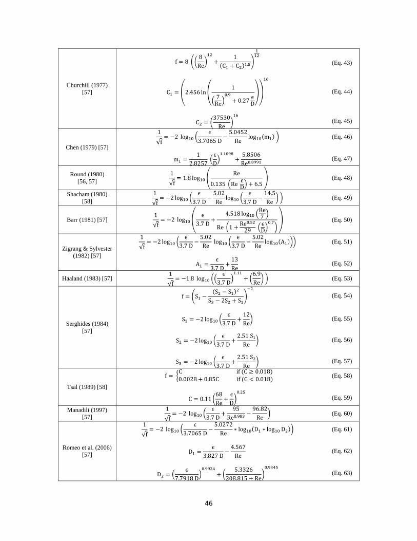
46
Churchill (1977)
[57]
f = 8 ((8
Re)
12
+1
(C1 + C2)1.5)
112
(Eq. 43)
C1 = (2.456 ln (1
(7
Re)
0.9
+ 0.27ϵD
))
16
(Eq. 44)
C2 = (37530
Re)
16
(Eq. 45)
Chen (1979) [57]
1
√f= −2 log10 (
ϵ
3.7065 D−
5.0452
Relog10(m1) ) (Eq. 46)
m1 =1
2.8257 (
ϵ
D)
1.1098
+5.8506
Re0.8991 (Eq. 47)
Round (1980)
[56, 57]
1
√f= 1.8 log10 (
Re
0.135 (Re ϵD
) + 6.5 ) (Eq. 48)
Shacham (1980)
[58]
1
√f= −2 log10 (
ϵ
3.7 D−
5.02
Relog10 (
ϵ
3.7 D−
14.5
Re) ) (Eq. 49)
Barr (1981) [57] 1
√f= −2 log10 (
ϵ
3.7 D+
4.518 log10 (Re7
)
Re (1 +Re0.52
29 (
ϵD
)0.7
) ) (Eq. 50)
Zigrang & Sylvester
(1982) [57]
1
√f= −2 log10 (
ϵ
3.7 D−
5.02
Re log10 (
ϵ
3.7 D−
5.02
Relog10(A1))) (Eq. 51)
A1 =ϵ
3.7 D+
13
Re (Eq. 52)
Haaland (1983) [57] 1
√f= −1.8 log10 ((
ϵ
3.7 D)
1.11
+ (6.9
Re) ) (Eq. 53)
Serghides (1984)
[57]
f = (S1 −(S2 − S1)2
S3 − 2S2 + S1)
−2
(Eq. 54)
S1 = −2 log10 (ϵ
3.7 D+
12
Re) (Eq. 55)
S2 = −2 log10 (ϵ
3.7 D+
2.51 S1
Re) (Eq. 56)
S3 = −2 log10 (ϵ
3.7 D+
2.51 S2
Re) (Eq. 57)
Tsal (1989) [58]
f = {C if (C ≥ 0.018)0.0028 + 0.85C if (C < 0.018)
(Eq. 58)
C = 0.11 (68
Re+
ϵ
D)
0.25
(Eq. 59)
Manadili (1997)
[57]
1
√f= −2 log10 (
ϵ
3.7 D+
95
Re0.983 −96.82
Re) (Eq. 60)
Romeo et al. (2006)
[57]
1
√f= −2 log10 (
ϵ
3.7065 D−
5.0272
Re∗ log10(D1 ∗ log10 D2)) (Eq. 61)
D1 =ϵ
3.827 D−
4.567
Re (Eq. 62)
D2 = (ϵ
7.7918 D)
0.9924
+ (5.3326
208.815 + Re)
0.9345
(Eq. 63)

47
Sonnad-Goudar
(2006) [57]
1
√f= 0.8686 ln (
0.4587 Re
GG
G+1
) (Eq. 64)
G = 0.124 Reϵ
D+ ln (0.4587 Re) (Eq. 65)
Buzelli (2008) [57]
1
√f= B1 − (
B1 + 2 log10 (B2Re
)
1 +2.18B2
) (Eq. 66)
B1 =(0.744 ln(Re)) − 1.41
(1 + 1.32 √ϵD
)
(Eq. 67)
B2 =ϵ
3.7 D Re + 2.51 B1 (Eq. 68)
Goudar-Sonnad
(2008) [58]
1
√f= a [ln (
d
q) + δCFA] (Eq. 69)
a =2
ln(10 ) (Eq. 70)
b =ϵ
3.7 D (Eq. 71)
d =ln(10)
5.02 Re (Eq. 72)
s = bd + ln (d) (Eq. 73)
q = ss
s+1 (Eq. 74)
g = bd + ln (d
q) (Eq. 75)
z =q
g (Eq. 76)
δLA =g
g + 1 z (Eq. 77)
δCFA = δLA (1 +
z2
(g + 1)2 + (z3
) (2g − 1)) (Eq. 78)
Avci & Karagoz
(2009) [57]
f =6.4
(ln(Re) − ln (1 + 0.01 ReϵD
(1 + 10 √ϵD
)))
2.4 (Eq. 79)
Papaevangelou et
al. (2010) [57] f =
0.2479 − 0.0000947 (7 − log10 Re)4
(log10 (ϵ
3.615 D+
7.366Re0.9142))
2 (Eq. 80)
Brkic a (2011) [57]
1
√f= −2 log10 (10−0.4343 β +
ϵ
3.71 D) (Eq. 81)
β = lnRe
1.816 ln (1.1 Re
ln(1 + 1.1 Re))
(Eq. 82)
Brkic b (2011) [57] 1
√f= −2 log10 (
2.18 β
Re+
ϵ
3.71 D) (Eq. 83)

48
𝛽 is (Eq. 82)
Danish et al (2011)
[55]
1
√f= C0 −
1.73718 C0 ln(C0)
1.73718 + C0+
2.62122 C0[ln(C0)]2
(1.73718 + C0)3
+3.03568 C0 [ln(C0)]3
(1.73718 + C0)4
(Eq. 84)
C0 = 4 log10(Re) − 0.4 (Eq. 85)
Fang (2011) [58] f = 1.613 [ln (0.234 (ϵ
D)
1.1007
−60.525
Re1.1105 +56.291
Re1.0712)]−2
(Eq. 86)
Ghanbari et al.
(2011) [57] f = [−1.52 log10 ((
ϵD
7.21)
1.042
+ (2.731
Re)
0.9152
)]
−2.169
(Eq. 87)
Li et al. (2011) [59]
f = 4Cf (Eq. 88)
Cf = −0.0015702
ln(Re)+
0.3942031
ln(Re)2 +2.5341533
ln(Re)3 (Eq. 89)
Morrison (2013)
[14] Cf = [
0.0076 (3170
Re)
0.165
1 + (3170
Re)
7.0 ] +16
Re (Eq. 90)
Shaikh et al. (2015)
[60]
f = 0.25 [log (2.51
α Re+
ϵ
3.7 D)]
−2
(Eq. 91)
α = [1.14 − 2 log10 (ϵ
D)]
−2
(Eq. 92)
Table A.2. Mixture viscosity correlations review.
Author Correlation
Einstein (1906) [15] μe
μc
= 1 + 2.5ϕ (Eq. 93)
Taylor (1932) [61]
μe
μc
= 1 + 2.5ϕA (Eq. 94)
A = [μc + 2.5μd
2.5μc + 2.5μd
] (Eq. 95)
Levinton and
Leighton (1936)
[62]
μe
μc
= exp [2.5A ∗ (ϕ + ϕ53 + ϕ
113 )] (Eq. 96)
𝐴 𝑖𝑠 (Eq. 95)
Guth and Simha
(1936) [16]
μe
μc
= 1 + 2.5ϕ + 14.1ϕ2 (Eq. 97)
Vand (1948) [15] μe
μc
= exp (2.5ϕ
1 − 0.609ϕ) (Eq. 98)
Brinkman and
Roscoe (1952) [63]
μe
μc
= (1 − ϕ)−2.5 (Eq. 99)
Vermuelen et al.
(1955) [64]
μe
μc
=1
1 − ϕ [ 1 +
1.5ϕμd
μc +μd
] (Eq. 100)
Maron-Pierce
(1956) [65]
μe
μc
= (1 −ϕ
ϕmax)
−2
(Eq. 101)
Dougherty &
Krieger (1959) [65]
μe
μc
= (1 −ϕ
ϕmax)
−2.5ϕmax
(Eq. 102)
Eiler (1962) [66] μe
μc
= [1 + 2.5ϕ(1 −αEϕ)−1]2 (Eq. 103)
Thomas (1965) [15] μe
μc
= [1 + 2.5ϕ + 10.05ϕ2 + 0.00273 exp(16.6ϕ)] (Eq. 104)
Chong et al. (1971)
[66]
μe
μc
= [1 + 0.75ϕ
ϕmax(1 −
ϕ
ϕmax)
−1
]
2
(Eq. 105)

49
Furuse (1972) [64] μe
μc
=1 + 0.5ϕ
(1 − ϕ)2 (Eq. 106)
Yaron and Gal-Or
(1972) [67]
μe
μc
= 1 + ϕ [5.5 [4 𝜙7 + 10 − (
8411
) 𝜙2 + (4𝐾
) (1 − 𝜙7)]
10(1 − ϕ10) − 25ϕ3(1 − ϕ4) + (10K
) (1 − ϕ3)(1 − ϕ7)] (Eq. 107)
K =μc
μd (Eq. 108)
Choi and
Schowalter (1975)
[67]
μe
μc
= 1 + ϕ [2(5K + 2) − 5(K − 1)ϕ7
4(K + 1) − 5(5K + 2)ϕ3 + 42Kϕ5 − 5(5K − 2)ϕ7 + 4(K − 1)ϕ10 ] (Eq. 109)
Barnea and Mizrahi
(1975) [61]
μe
μc
= B′ [
23
B′ +μdμc
B′ +μdμc
] (Eq. 110)
B′ = exp [5ϕA′
3(1 − ϕ)] (Eq. 111)
A′ = [μc + 2.5μd
2.5μc + 2.5μd
] (Eq. 112)
Phan-Thien & Pham
(1997) [67] (μe
𝜇𝑐)
25
[2 (μeμc
) + 5 (μdμc
)
2 + 5 (μdμc
)]
35
= (1 − ϕ)−1 (Eq. 113)
Pal (2001) [65] μe
μc
(2μeμc
+ 5K
2 + 5K)
32
= exp(2.5ϕ) (Eq. 114)
Pal (2001) [65] μe
μc
(2μeμc
+ 5K
2 + 5K)
32
= [1 +1.25 𝜙
1 −𝜙
𝜙𝑚
]
2
(Eq. 115)
Pal (2001) [65] μe
μc
(2 (μeμc
) + 5K
2 + 5K)
32
= [1 −ϕ
ϕm]
−2
(Eq. 116)
Pal (2001) [65] μe
μc
(2μeμc
+ 5K
2 + 5K)
32
= [1 +0.75 (
ϕϕm
)
1 − (ϕ
ϕm)
]
2
(Eq. 117)
9.2.Appendix B

50
Figure B.1. Experimental pressure gradient against calculated with OLGA for each pattern within ±30% error.