Preservation of Electronic Records Workshop

COMMUNICATIONS IN COMPUTATIONAL PHYSICSVol. 1, No. 6, pp. 1010-1042

Commun. Comput. Phys.December 2006

On Integral Equation and Least Squares Methods

for Scattering by Diffraction Gratings

Tilo Arens1, Simon N. Chandler-Wilde2,∗ and John A. DeSanto3

1 Mathematisches Institut II, Univeristat Karlsruhe, 76128 Karlsruhe, Germany.2 Department of Mathematics, University of Reading, Whiteknights, PO Box 220,Berkshire RG6 6AX, United Kingdom.3 Mathematical and Computer Sciences, Colorado School of Mines, Golden, CO80401, USA.

Received 5 December 2005; Accepted (in revised version) 8 May 2006

Abstract. In this paper we consider the scattering of a plane acoustic or electromagneticwave by a one-dimensional, periodic rough surface. We restrict the discussion to the case whenthe boundary is sound soft in the acoustic case, perfectly reflecting with TE polarization in theEM case, so that the total field vanishes on the boundary. We propose a uniquely solvablefirst kind integral equation formulation of the problem, which amounts to a requirementthat the normal derivative of the Green’s representation formula for the total field vanishon a horizontal line below the scattering surface. We then discuss the numerical solution byGalerkin’s method of this (ill-posed) integral equation. We point out that, with two particularchoices of the trial and test spaces, we recover the so-called SC (spectral-coordinate) and SS(spectral-spectral) numerical schemes of DeSanto et al., Waves Random Media, 8, 315-414,1998. We next propose a new Galerkin scheme, a modification of the SS method that we termthe SS∗ method, which is an instance of the well-known dual least squares Galerkin method.We show that the SS∗ method is always well-defined and is optimally convergent as the sizeof the approximation space increases. Moreover, we make a connection with the classicalleast squares method, in which the coefficients in the Rayleigh expansion of the solution aredetermined by enforcing the boundary condition in a least squares sense, pointing out thatthe linear system to be solved in the SS∗ method is identical to that in the least squaresmethod. Using this connection we show that (reflecting the ill-posed nature of the integralequation solved) the condition number of the linear system in the SS∗ and least squaresmethods approaches infinity as the approximation space increases in size. We also providetheoretical error bounds on the condition number and on the errors induced in the numericalsolution computed as a result of ill-conditioning. Numerical results confirm the convergenceof the SS∗ method and illustrate the ill-conditioning that arises.

Key words: Helmholtz equation; first kind integral equation; spectral method; condition number.

∗Correspondence to: S. N. Chandler-Wilde, Department of Mathematics, University of Reading,Whiteknights, Berkshire RG6 6AX, United Kingdom. Email: [email protected]

http://www.global-sci.com/ 1010 c©2006 Global-Science Press

T. Arens, S. N. Chandler-Wilde and J. A. DeSanto / Commun. Comput. Phys., 1 (2006), pp. 1010-1042 1011

1 Introduction

We consider the scattering of a plane acoustic or electromagnetic wave by a perfectlyreflecting, periodic surface. Adopting Cartesian coordinates Oxyz we assume that thesurface is invariant in the y direction and periodic in the x direction, specified by theequation z = f(x), for some given continuous function f . The mathematical problemto be solved is two-dimensional. We assume throughout that the incident wave is time-harmonic (e−iωt time dependence), so that the total wave field ut is a solution of theHelmholtz equation

∆ut + k2 ut = 0 in Ω, (1.1)

where Ω := r = (x, z) ∈ R2 : z > f(x) is that part of the Oxz plane above the scattering

surface. Throughout, we will assume that f is periodic with period L > 0 and that theincident field ui is the plane wave

ui(r) = exp(ik[x sin θ − z cos θ]), (1.2)

where θ is the angle of incidence, measured from the z-axis, with −π/2 < θ < π/2. It isthe goal to determine the scattered field u := ut − ui given the boundary condition

ut = ui + u = 0 on ∂Ω, (1.3)

where ∂Ω = (x, f(x)) : x ∈ R, and given that an appropriate radiation condition on uholds, expressing that u is outgoing from ∂Ω. This problem models scattering of electro-magnetic plane waves by a perfectly conducting diffraction grating in the TE polarizationcase. The same mathematics models acoustic scattering by a one-dimensional periodicsound soft surface.

Many different methods have been proposed for solving this problem. Alternativeboundary integral equation methods to those proposed here are discussed in [1, 29, 35],standard differential equation (coupled-mode) based methods in [4, 31, 33], a coordinate-transformation-based differential equation method in [20, 21], and a method of variationof boundaries based on analytic continuation arguments in [5]. Many different specificsurface examples are available [12] as well as the first treatment of the problem usingspectral methods [13]. An extensive recent review of many of the different computationalmethods available is made in [14]. A classical method for solving this problem, on which wethrow new light in Section 5, is the least squares method [28, 30], in which the scatteredfield is expressed as a linear combination of solutions of the Helmholtz equation (theRayleigh expansion (2.1) below) and the coefficients in this expansion are determined byrequiring that the boundary condition holds in a least squares sense. We note that, in thecontext of determining eigenfunctions of the Laplacian in 2D domains, the least squaresmethod has recently been revived by Betcke and Trefethen [3]. The problem can also betackled via a variational formulation in a part of the domain, truncated by the Rayleighexpansion which provides a non-local boundary condition, with the variational problemsolved numerically by standard finite element methods (see e.g. [2, 17,18]).

1012T. Arens, S. N. Chandler-Wilde and J. A. DeSanto / Commun. Comput. Phys., 1 (2006), pp. 1010-1042

In Section 2 of the paper we formulate the scattering problem mathematically andderive the equivalent first kind integral equation formulation which is the basis of three ofthe numerical methods that we describe later in the paper.

In Section 3 we establish mapping properties of the integral operator that occurs inthis formulation and properties of its adjoint operator, these properties key to analysingthe stability and convergence of two of the numerical methods we will discuss. In thissection we also study sets of basis functions which may be used to develop expansionsfor the solution of the integral equation. As a consequence of the mapping properties ofthe integral operators it follows, in particular, that one possible set of basis functions,the so-called topological basis functions, used in the numerical methods for diffractiongratings discussed in [15], are linearly independent and are complete in the space of squareintegrable functions.

The numerical solution, via Galerkin methods, of the first kind integral equation for-mulation we propose is the subject of Section 4. We point out that, applying a Galerkinscheme with a pulse basis (piecewise constant basis functions as the trial space) leads, af-ter approximation of the integrals involved, to the version of the SC method implementedin [13, 15]. Applying a Galerkin method and expanding the solution in topological ba-sis functions leads to the SS method of [15, 16]. The effectiveness of these methods forscattering by one-dimensional periodic surfaces has been investigated by careful numericalexperiments in [15, 16], the experiments suggesting that both methods are very fast andaccurate within certain parameter domains but can become ill-conditioned for surfaceswith large slopes. We note further that no convergence proofs were given.

In Section 4 we also propose a new method, which we term the SS∗ method, basedon a modification of the topological basis functions. As we point out, with this particularchoice of basis functions the Galerkin method is an instance of the so-called dual leastsquares method [24]. The self-regularization properties of this method are well-known(see [24] and the references therein). Applying arguments from the theory of the dualleast squares method [24] we are able to establish that the SS∗ method is convergent.Further we are able to establish precise estimates for the conditioning of the linear systemto be solved, and how this conditioning depends on the surface and on the dimension ofthe approximation space, obtaining an upper bound on the loss of accuracy arising fromevaluation of matrix entries by numerical quadrature.

In Section 5 we make connections between the SS∗ method we propose and the classicleast squares method, in which the coefficients in the Rayleigh expansion (equation (2.1)below) for the scattered field are determined directly by the requirement that the boundarycondition that the total field vanish is required to hold in a least squares sense. We describea straightforward implementation of the least squares method which leads to solving theidentical linear system to that solved in the SS∗ method. Given this connection, we areable to apply the results of Section 4 to deduce new information about the least squaresmethod. In particular, we prove that the method is convergent in all cases (previousanalyses, [28,30], exclude certain combinations of the angle of incidence and the period).We also provide the first proof that the condition number of the matrix becomes unbounded


as N (the dimension of the approximation space) tends to infinity, and we provide an upperbound for the condition number as a function of N , the wavenumber, and the maximumsurface height.

In the final Section 6 we present some numerical experiments, for scattering by si-nusoidal surfaces, using parameter values (surface elevation, period, angle of incidence)selected from the examples for which results were computed previously in [15]. We com-pare the SC, SS, SS∗ and least squares methods, using a different type of method (thesuper-algebraically convergent Nystrom method of [29], based on solving a boundary inte-gral equation of the second kind), to provide accurate results for comparison. The limitednumerical results illustrate why the methods we study in this paper are interesting fornumerical computation, namely that, at least in some cases, very accurate results are ob-tained with the ratio of number of degrees of freedom to arc-length of boundary in therange 1-2. This compares very well with conventional boundary element methods where aratio 5-10 is usually recommended in the engineering literature as the minimum require-ment for acceptable accuracy. Our limited numerical results also suggest that the SS∗ andleast squares methods have similar accuracy, and are more robust and reliable than theSC and the SS methods. This is in line with the theoretical results of Sections 4 and 5,where we are able to provide rigorous convergence proofs and error estimates for the SS∗

and least squares methods, while it is not clear theoretically that the SC and SS methodsneed be convergent as the number of degrees of freedom increases; indeed the numericalresults suggest that these methods may not be convergent in all cases. We also use thissection to investigate the conditioning of the linear system solved in the SS∗ and leastsquares methods. Our calculations confirm the ill-conditioning as N → ∞. Indeed thecondition number ultimately grows exponentially with N as our upper bound on the con-dition number predicts, though our upper bound overpredicts the rate of this exponentialgrowth for the examples we look at.

We close this introduction with a brief list of notations used in the paper. Throughoutλ = 2π/k is the wavelength. The set of measurable functions that are square integrableon (−L/2, L/2), usually denoted as L2(−L/2, L/2), will be abbreviated as X. The partof ∂Ω corresponding to a single period from −L/2 to L/2 will be denoted by Γ, i.e.Γ := r = (x, f(x)) : −L/2 ≤ x ≤ L/2. Similarly, R

2L denotes the part of the plane (R2)

with −L/2 < x < L/2, i.e. R2L := r ∈ R

2 : −L/2 < x < L/2. It is also useful to havea notation for the finite horizontal line of height h in R

2L, namely Γh := (x, h) : −L/2 ≤

x ≤ L/2.

2 The scattering problem and a first kind integral equation

Given that the incident field ui is the plane wave (1.2), we seek a scattered field u and totalfield ut = u+ui which satisfy the Helmholtz equation (1.1) in Ω and the boundary condition(1.3). To capture fully the physics of the problem and ensure uniqueness of solution it isnecessary to impose additional constraints, expressed in terms of the following definitions.


Definition 2.1. A function u ∈ C(Ω) is said to be quasi-periodic (or Floquet periodic)with period L and phase-shift µ if

u(x+ L, z) = exp(iµL)u(x, z),

for r = (x, z) ∈ Ω.

Let f− := min f and f+ := max f , so that

f− ≤ f(x) ≤ f+.

Definition 2.2. A function u ∈ C2(Ω) is said to satisfy the Rayleigh expansion radiationcondition (RERC) if, for some complex constants un, which we will call the Rayleighcoefficients,

u(r) =∑

n∈Z

un exp(ik[αnx+ βnz]), for z > f+, (2.1)

where αn := sin θ + nλ/L (the Bragg condition) and

βn :=

√

1 − α2n, |αn| ≤ 1,

i√

α2n − 1, |αn| > 1.

The incident field is quasi-periodic with period L and phase-shift µ = k sin θ, andit is appropriate, given the periodicity of f , to require that the scattered field u is alsoquasi-periodic with the same period and phase shift. It then follows, given that u satisfiesthe Helmholtz equation in every half-plane above ∂Ω, that, for z > f+, u is a linearcombination of plane waves and inhomogeneous plane waves of the form exp(ik[αnx±βnz]).Discarding those waves which propagate downwards or increase exponentially with z leadsto the requirement that u satisfy the RERC.

The complete formulation of the scattering problem is thus as follows. Note that weassume in this problem specification, to simplify later mathematical analysis, that theboundary curve ∂Ω has continuously varying tangent and curvature, equivalently that flies in the set of functions f ∈ C2(R). For an analysis, including a proof of uniquenessand existence of solution, of the case when f is merely Lipschitz continuous see [18].

Problem 2.1. Given an L-periodic function f ∈ C2(R) and an incident field ui, definedby (1.2), find u ∈ C2(Ω)∩C(Ω), quasi-periodic with period L and phase-shift µ = k sin θ,such that ut := u+ ui satisfies the Helmholtz equation (1.1) and the boundary condition(1.3), and u satisfies the RERC.

Remark 2.1. It is a well known result (e.g. [22, 34]) that Problem 2.1 has exactly onesolution, and that the gradient of this solution is continuous up to the boundary ∂Ω, sothat u ∈ C1(Ω), which allows the application below of Green’s theorem. It is perhaps lesswell known that the assumption of quasi-periodicity is not required to ensure uniqueness.It is shown in [9] that a weaker radiation condition than the RERC, the upward propagating


radiation condition (UPRC) of [7], implies uniqueness of solution for scattering by generalrough surfaces, if it is assumed that u is bounded in every horizontal strip above ∂Ω. Wealso point out that it is shown in [8] that the weaker UPRC combined with an assumptionof quasi-periodicity is equivalent to the RERC.

We proceed to derive a first kind integral equation formulation for Problem 2.1 viaapplications of Green’s theorem. For this purpose, we introduce the quasi-periodic Green’sfunction for the Helmholtz equation Gp, defined by

Gp(r, r0) :=i

2kL

∑

n∈Z

1

βnexp(ik[αn(x− x0) + βn|z − z0|]), (2.2)

for all r = (x, z), r0 = (x0, z0) with r−r0 not a multiple of the vector (L, 0). Of course, Gpis only well-defined in the case that βn 6= 0 for all n ∈ Z and, for the moment, we assumethat this is the case. We note that the quasi-periodic Green’s function can be written inmany equivalent forms, for example as the sum of Hankel functions

Gp(r, r0) =i

4

∑

n∈Z

exp(ikα0nL)H(1)0 (k|r − rn|),

where rn := (x0 + nL, z0). These representations and others more suited for numericalcalculation are derived and discussed in [15, 27]. Note that it is clear from either of theabove representations that Gp(r, r0), as a function of r, is quasi-periodic with period Land phase shift µ = k sin θ.

Now let D ⊂ R2L denote any domain in which the divergence theorem holds. Further,

let ν denote the outward drawn normal to D. Then, for any solution u ∈ C2(D) ∩C1(D)of the Helmholtz equation, there holds

∫

∂D

Gp(r, r0)∂u

∂ν(r0) −

∂Gp(r, r0)

∂ν(r0)u(r0)

ds(r0) =

u(r), r ∈ D,

0, r ∈ R2L \D.

(2.3)

Possible choices for the domain D are D+H2

:= r = (x, z) ∈ R2L : f(x) < z < H2, with

H2 > f+, and D−H1

:= r = (x, z) ∈ R2L : H1 < z < f(x), with H1 < f−. If Green’s

formula (2.3) is applied in D+H2

or D−H1

to a field u that is quasi-periodic, then the integralsover the vertical lines x = −L/2 and x = L/2 cancel. In particular, suppose that H1 < f−and H2 > f+. Then, with n denoting the downward drawn normal to Γ, applying (2.3) toui in D−

H1we obtain that, for r = (x, z) ∈ R

2L,

∫

Γ

Gp(r, r0)∂ui

∂n(r0) −

∂Gp(r, r0)

∂n(r0)ui(r0)

ds(r0)

+

∫

ΓH1

Gp(r, r0)∂ui

∂z0(r0) −

∂Gp(r, r0)

∂z0ui(r0)

dx0 =

−ui(r), if H1 < z < f(x),

0, if z > f(x).(2.4)


Similarly, applying (2.3) to u in D+H2

yields

∫

Γ

Gp(r, r0)∂u

∂n(r0) −

∂Gp(r, r0)

∂n(r0)u(r0)

ds(r0)

−

∫

ΓH2

Gp(r, r0)∂u

∂z0(r0) −

∂Gp(r, r0)

∂z0u(r0)

dx0 =

0, if z < f(x),

u(r), if f(x) < z < H2.(2.5)

Since u satisfies the RERC and using the definition of the Green’s function we see that,for z < H2, the second integral in (2.5) has the value

∫

ΓH2

Gp(r, r0)∂u

∂z0(r0) −

∂Gp(r, r0)

∂z0u(r0)

dx0

=

∫

ΓH2

∑

m∈Z

um exp(ik[αmx0 + βmH2])

Gp(r, r0) ikβm −∂Gp(r, r0)

∂z0

dx0

=−1

2L

∫ L/2

−L/2

∑

m∈Z

∑

n∈Z

um exp

(

ik

[

αnx+ βn(H2 − z) + βmH2 + (m− n)λx0

L

])(

βmβn

− 1

)

dx0

= 0.

A similar calculation yields that the second integral in (2.4) also vanishes, provided z > H1.Thus, adding (2.4) to (2.5) and applying the boundary condition (1.3) yields that

∫

ΓGp(r, r0)

∂ut

∂n(r0) ds(r0) =

u(r), if z > f(x),

−ui(r), if z < f(x),(2.6)

the lower part of this equation often referred to as the extinction theorem [32].

We see from (2.6) that, to compute the scattered field we need only find the normalderivative of the total field on Γ. Equation (2.6) provides integral equations for determiningthis normal derivative. In particular, we shall compute numerical solutions by solving afirst kind integral equation obtained by differentiating (2.6). For z < f− and r0 ∈ Γ itis clear from the definition that Gp(r, r0) is continuously differentiable with respect to z.Thus we can take the derivative on both sides of (2.6) with respect to z, exchanging theorder of differentiation and integration, to obtain the integral equation

−∂ui

∂z(r) =

∫

Γ

∂Gp(r, r0)

∂z

∂ut

∂n(r0) ds(r0), r ∈ ΓH , (2.7)

which holds for every H < f−.

We will rewrite (2.7) as an integral equation on the interval (−L/2, L/2). For −L/2 ≤


x ≤ L/2, −L/2 ≤ x0 ≤ L/2, set

ϕ(x0) :=1

k

∂ut(r0)

∂n

∣

∣

∣

r0=(x0,f(x0))

√

1 + f ′(x0)2,

ψ(x) := −2

k

∂ui(r)

∂z

∣

∣

∣

r=(x,H)= 2iβ0 exp(ik[α0x− β0H]), (2.8)

K(x, x0) := 2L∂Gp(r, r0)

∂z

∣

∣

∣

r=(x,H), r0=(x0,f(x0)).

Then (2.7) can be rewritten as the integral equation

ψ(x) =1

L

∫ L/2

−L/2K(x, x0)ϕ(x0)dx0, −L/2 ≤ x ≤ L/2, (2.9)

or, in operator form,

Dϕ = ψ, (2.10)

where the integral operator D is defined by

Dϕ(x) :=1

L

∫ L/2

−L/2K(x, x0)ϕ(x0) dx0, −L/2 ≤ x ≤ L/2. (2.11)

Explicitly, the kernel K(x, x0) is given by

K(x, x0) =∑

n∈Z

exp(ik[αn(x− x0) + βn(f(x0) −H)]). (2.12)

The benefit of differentiating (2.6) is that (2.12) is well-defined even in the case thatβn = 0 for some n ∈ Z. Our derivation of (2.9) assumed that βn 6= 0 for all n ∈ Z.However, using the result that the solution to Problem 2.1 depends continuously on theangle of incidence [22], it follows that (2.9) holds even when βn = 0 for some n, by firstperturbing θ slightly to make βn 6= 0, so that (2.9) holds, and then taking the limit as thisperturbation tends to zero.

In the results shown below we shall compute ϕ by solving (2.9). Note that (2.9) hasexactly one solution in X = L2(−L/2, L/2). To see this, note first that the derivationabove shows that (2.9) does have a solution, namely the normal derivative of the totalfield that satisfies Problem 2.1. Further, we show in the next section that the operator Dis injective so that this solution is unique.

Once ϕ is obtained, and provided βn 6= 0 for all n ∈ Z, the scattered field is given by(2.6), which can be written as

u(r) = k

∫ L/2

−L/2Gp(r, (x0, f(x0)))ϕ(x0)dx0. (2.13)


An alternative representation for the scattered field can be obtained by reflecting equation(2.6) in the line z = h, for some h < f−, to obtain that

k

∫ L/2

−L/2Gp(r, (x0, 2h− f(x0)))ϕ(x0)dx0 = − exp(ik[α0x− β0(2h − z)]),

for 2h − z < f(x). In particular this equation holds for z > f(x). Thus, subtracting theequation from (2.13), we find that

u(r) = − exp(ik[α0x− β0(2h− z)]) + k

∫ L/2

−L/2Gp,h(r, (x0, f(x0)))ϕ(x0)dx0, (2.14)

for z > f(x), whereGp,h(r, r0) := Gp(r, r0) −Gp(r, r0

′), (2.15)

and r0′ := (x0, 2h− z0) denotes the reflection of r0 = (x0, z0) in the line z = h. Note that

Gp,h is the quasi-periodic Dirichlet Green’s function for the upper half-plane z > h, sinceGp,h(r, r0) = 0 on z = h.

The advantage of (2.14) compared to (2.13) is that, while Gp is undefined when βn = 0for some n, the definition of Gp,h can be extended to this case by perturbing θ slightly sothat βn 6= 0 and then taking the limit in (2.15) as this perturbation tends to zero. From(2.2) and (2.15) we see that, explicitly, this leads to the equation

Gp,h(r, r0) =i

2kL

∑

n∈Z

exp(ikαn(x− x0))cn(z, z0), (2.16)

where

cn(z, z0) :=

1βn

[exp(ikβn|z − z0|) − exp(ikβn(z + z0 − 2h))], if βn 6= 0,

ik(|z − z0| − (z + z0 − 2h)), if βn = 0.

Our derivation of (2.14) assumed, implicitly, that βn 6= 0 for every n. But, in the sameway we argued that (2.9) holds when βn = 0 for some n, it follows that (2.14) holds inthis case too.

From (2.2) and (2.13) we see that the coefficients in the Rayleigh expansion represen-tation for u(r), equation (2.1), are given by

un =i

2Lβn

∫ L/2

−L/2exp(−ik[αnx0 + βnf(x0)])ϕ(x0)dx0, (2.17)

at least in the case that βn 6= 0 for all n ∈ Z. If βm = 0 for some m ∈ Z we see, from thecontinuous dependence of both u and βn on θ, that (2.17) still holds for n 6= m.

We can also find expressions for the coefficients un from (2.16) and (2.14). For z > z0,

cn(z, z0) = −2ik(z0 − h) exp(ikβn(z − h)) sinc (kβn(z0 − h)),


where

sinc t :=

sin t

t, t 6= 0,

1, t = 0.

Thus it follows from (2.16) and (2.14) that

un = − exp(−2ikβ0h)δ0,n

+k

Le−ikβnh

∫ L/2

−L/2e−ikαnx0(f(x0) − h)sinc (kβn(f(x0) − h))ϕ(x0)dx0, (2.18)

where δm,n is the Kronecker delta, with δmn = 1 if m = n, = 0 otherwise. In particular,in the case that βn = 0, (2.18) gives that

un =k

L

∫ L/2

−L/2exp(−ikαnx0)(f(x0) − h)ϕ(x0)dx0. (2.19)

Note that, in deriving (2.18), we have assumed that h < f−, but in fact, as the left andright hand sides of (2.18) are both analytic as functions of h in the whole complex plane,it follows by analytic continuation that (2.18) and its special case (2.19) in fact hold forall (real or complex!) values of h. We note that the expression (2.18) for the Rayleighcoefficients appears to be new.

3 Basis functions and properties of the integral operators

An understanding of the integral operatorD relies to a great extent on properties of certainsets of basis functions for the space X = L2(−L/2, L/2), the set of square integrablefunctions, a Hilbert space with the inner product

〈φ,ψ〉 :=1

L

∫ L/2

−L/2φ(x)ψ(x) dx

and norm ‖φ‖ := 〈φ, φ〉1/2. A standard set of basis functions for X is the Fourier basis.Taking into account that we wish to represent quasi-periodic functions, it is natural toshift the standard Fourier basis slightly, using the orthogonal basis functions φn, definedby

φn(x) := exp(ik αn x), −L/2 ≤ x ≤ L/2, n ∈ Z. (3.1)

The functions φn, n ∈ Z, form a complete orthonormal system in X, so that

〈φn, φm〉 = δmn,

where δmn is the Kronecker delta. They appear quite naturally in connection with theintegral operator D: from (2.11) and (2.12) we obtain that

Dϕ(x) =∑

n∈Z

σn 〈ϕ,ψn〉φn(x), (3.2)


where

σn := exp(ikβn(f− −H)), ψn(x) := exp(

ik [αn x− βn(f(x) − f−)])

.

We point out that |ψn(x)| ≤ 1, with equality at the point x where f(x) = f−, and withequality for all x in the case that |αn| ≤ 1. Note also that |σn| ≤ 1, with equality for|αn| ≤ 1, and that σn ∼ exp(−k(f− −H)|αn|) as n→ ±∞.

Let D∗ denote the L2-adjoint of the operator D, defined by the equation

〈Dϕ,ψ〉 = 〈ϕ,D∗ψ〉, for all φ,ψ ∈ X. (3.3)

Explicitly,

D∗ψ(x) =1

L

∫ L/2

−L/2K(x0, x)ψ(x0)dx0, −L/2 ≤ x ≤ L/2,

for ψ ∈ X, from which it follows that

D∗ψ =∑

n∈Z

σn 〈ψ, φn〉 ψn. (3.4)

We note that, in the case when Γ is flat, i.e. f− = f(x) = f+, it holds that ψn = φn.It then follows from (3.2) and (3.4) that φn is an eigenfunction of both D and D∗, witheigenvalues σn and σn, respectively, and that |σn| : n ∈ Z are the singular values of Dand D∗.

The numerical scheme we will propose for solving (2.9) will be a Galerkin scheme, basedon expanding the solution of the integral equation in a finite sum of the functions ψn, andwe will see in a moment that the set ψn : n ∈ Z is linearly independent and completein X. A closely related basis for X is the set of so-called topological basis functions [15],ψn : n ∈ Z, defined by

ψn(x) := exp(ik [αnx− βn(f(x) − f−)]).

We will also discuss, following [15], using these functions to expand the solution, leadingto the SS method of [15].

All three sets of basis functions are related to plane waves. Let vn(r) = exp(ik [αnx−βnz]), so that vn is either a downwards propagating plane wave or an evanescent wavedecaying exponentially as z decreases. Then φn is a multiple of vn restricted to ΓH , whileψn is a multiple of vn restricted to Γ. The functions ψn are also related to restrictions ofplane waves on Γ. Let wn be the plane wave travelling in the opposite direction to vn,i.e. wn(r) = exp(ik [−αnx+ βnz]). Then ψn is a multiple of the complex conjugate of wnrestricted to Γ.

We will now proceed by establishing some crucial properties of the sets of basis func-tions, and in fact giving some justification to the term basis function. Our first result wasproved previously, for the case in which βn 6= 0 for all n ∈ Z, in [23], this paper makingprecise and completing the earlier argument in [30]. See [6, 36] for related comments onthe completeness of plane wave bases in the case of non-periodic surfaces.


Lemma 3.1. The set of functions ψn : n ∈ Z is complete in X.

Proof. Let ϕ ∈ X and assume that

〈ϕ,ψn〉 =1

L

∫ L/2

−L/2ϕ(x)ψn(x) dx = 0, n ∈ Z.

Define φ ∈ L2(Γ) by

φ(r0) =kϕ(x0)

√

1 + f ′(x0)2, r0 = (x0, z0) ∈ Γ,

choose h < f−, and consider the function v, defined by

v(r) :=

∫

ΓGp,h(r, r0)φ(r0) ds(r0), z > h,

where Gp,h is the quasi-periodic Dirichlet Green’s function for the half-plane z > h, givenby (2.16). For h < z < f− it follows from (2.16) that, where dn(z) is defined by

dn(z) :=

1βn

[exp(−ikβnz) − exp(ikβn(z − 2h))], if βn 6= 0,

2ik(h − z), if βn = 0,

it holds that

v(r) =i

2L

∑

n∈Z

exp(ik[αnx+ βnf−])dn(z)

L/2∫

−L/2

ψn(x0)ϕ(x0)dx0 = 0.

Since solutions of the Helmholtz equation are analytic [10], it follows that v(r) = 0 forh < z < f(x). But v is a single layer potential with L2 density and so is continuous in R

2,so that v = 0 on ∂Ω. Further, v ∈ C2(Ω) and is quasiperiodic and satisfies the Helmholtzequation in Ω and the RERC. Thus, from the fact that Problem 2.1 has only one solution,it follows that v = 0 in Ω. However, from jump relations for single-layer potentials withL2 densities [11], it follows that

φ(r0) =∂v+

∂n(r0) −

∂v−

∂n(r0),

for almost all r0 ∈ Γ, where the superscripts + and − denote limiting values of the normalderivative as the boundary is approached from below and above, respectively. Thus ϕ = 0in X. This completes the proof.

Of course the significance of the completeness of ψn : n ∈ Z is that it means thatthe linear span of ψn : n ∈ Z is dense in X, i.e. that every function in X can be


approximated arbitrarily closely by finite linear combinations of the functions ψn. Inparticular, the solution, ϕ, of the integral equation (2.9) can be approximated in this way.

Since the topological basis functions ψn are so closely related to the functions ψn,precisely ψn is the restriction of a plane wave on Γ while ψn is the restriction to Γ of theplane wave travelling in exactly the opposite direction, the completeness in X of the setof topological basis functions, ψn : n ∈ Z, follows by symmetry from Lemma 3.1.

The previous lemma also has immediate consequences for the operator D defined inthe previous section.

Lemma 3.2. The operator D is injective.

Proof. Assume ϕ ∈ X and Dϕ = 0. Then all the Fourier coefficients of Dϕ vanish. Butthe series on the right hand side of (3.2) is exactly the Fourier expansion of Dϕ. It followsthat 〈ϕ,ψn〉 = 0 for all n ∈ Z. Thus, by Lemma 3.1, ϕ = 0 and the assertion is proved.

Lemma 3.3. The operator D∗ is injective.

Proof. Suppose that ψ ∈ X and D∗ψ = 0 and consider the double layer potential

v(r) := 2

∫

ΓH

∂Gp(r, r0)

∂z0ψ(x0) ds(r0),

for r = (x, z), z > H. Here Gp denotes the quasi-periodic Green’s function with θ replacedby −θ, and so αn replaced by αn := − sin θ+ nλ/L and βn replaced with βn :=

√

1 − α2n.

Then, from (2.2), it follows that, for z > H,

v(r) =1

L

∑

n∈Z

∫ L/2

−L/2exp(ik[αn(x− x0) + βn(z −H)])ψ(x0) dx0

=∑

n∈Z

exp(−ik[αnx− βn(z −H)])〈φn, ψ〉, (3.5)

since α−n = −αn and β−n = βn. In particular, for r = (x, f(x)), −L/2 < x < L/2, wehave

v(r) =∑

n∈Z

exp(−ik[αnx− βn(f(x) −H)])〈φn, ψ〉

and, comparing with (3.4), we see that this expression is equal to D∗ψ(x). Since D∗ψ = 0it follows that v = 0 on Γ. However, v ∈ C2(Ω) and is quasiperiodic and a solution to theHelmholtz equation in Ω, and v satisfies the RERC. Thus, from the uniqueness result forProblem 2.1, it follows that v = 0 in Ω and, by analytic continuation, that v(r) = 0 forz > H.

Thus and from (3.5), for z > H and m ∈ Z,

0 =1

L

∫ L/2

−L/2v(r)φm(x)dx =

∑

n∈Z

〈φm, φn〉 exp(ikβn(z −H))〈φn, ψ〉

= exp(ikβm(z −H))〈φm, ψ〉,


since φn : n ∈ Z is orthonormal, so that 〈φm, φn〉 = 0 for n 6= m. Thus 〈ψ, φm〉 =〈φm, ψ〉 = 0 for m ∈ Z. Since φn : n ∈ Z is complete, it follows that ψ = 0.

It is a standard result in functional analysis that if D is a bounded linear operator ona Hilbert space, then D is injective if and only if the range of D∗, the adjoint of D, isdense in X. Thus we have the following consequence of Lemmas 3.2 and 3.3.

Corollary 3.1. The operators D and D∗ have dense range.

Next note the following relationship between φn and ψn which will be key to theeffectiveness of the numerical scheme we propose. From (3.4), we have

D∗φn =∑

m∈Z

σm 〈φn, φm〉ψm.

But the functions φn are orthonormal. Thus

D∗φn = σn ψn. (3.6)

This relationship together with the injectivity of the operator D∗ has the followingconsequence for the functions ψn.

Corollary 3.2. The set of functions ψn : n ∈ Z is linearly independent.

Proof. Suppose that N ∈ N, that j1, j2, ..., jN ∈ Z and that

a1ψj1 + a2ψj2 + ...+ aNψjN = 0

for some constants a1, ..., aN . Then, by (3.6) and the linearity of D∗,

D∗(a1φj1 + a2φj2 + ...+ aNφjN ) = 0,

where am := am/σjm. Since D∗ is injective from Lemma 3.3, it follows that

a1φj1 + a2φj2 + ...+ aNφjN = 0.

Since φn : n ∈ Z is orthogonal and thus linearly independent, it follows that am = 0 form = 1, ..., N , so that am = 0 for m = 1, ..., N .

4 Galerkin methods for the first kind integral equation

The first kind integral equation (2.10), in common with all first kind integral equations withcontinuous or weakly singular kernels, is ill-posed, that is the inverse operator D−1, fromthe range of D onto X, is an unbounded operator. As a consequence, small changes in thefunction ψ in (2.10) and small changes to the operator D can lead to large changes in thesolution ϕ. Great care has to be taken when solving (2.10) numerically, in particular as D


will be approximated in the discretisation process. It is essential to use a numerical schemewhich incorporates regularisation, so that, at the discrete level, D−1 is approximated by abounded operator: see [19,24,26] for a clear exposition of these issues. It is well known thatcertain Galerkin methods for solving first kind integral equations are self-regularizing, i.e.they have inbuilt regularization properties [24]. We will discuss certain Galerkin methodsfor solving (2.10) in this section.

Given two finite subspaces XN , YN ⊂ X of dimension N , the Galerkin method for(2.10) consists of finding a solution φN ∈ XN of the variational equation

〈DϕN , ψ〉 = 〈ψ, ψ〉, for all ψ ∈ YN . (4.1)

Equation (4.1) is in fact equivalent to a finite system of simultaneous equations: given bases

x1, . . . ,xN of XN and y1, . . . ,yN of YN , respectively, and setting ϕN =∑N

n=1 a(N)n xn,

(4.1) can be reformulated as the system

N∑

n=1

〈Dxn,ym〉 a(N)n = 〈ψ,ym〉, m = 1, . . . , N. (4.2)

Various versions of the Galerkin method can be obtained by specific choices of thesubspaces XN and YN and their bases. Noting the representation (3.2) for Dϕ, we seethat a particularly convenient choice for YN is the space spanned by N distinct Fouriermodes, φj1 , ..., φjN . With this choice of YN it follows from (3.2) and (2.8), and sinceφn : n ∈ Z is orthonormal, that

〈Dxn,ym〉 = σjm 〈xn, ψjm〉 (4.3)

and〈ψ,ym〉 = 2iβ0 exp(−ikβ0H)δ0,jm , (4.4)

where δmn is the Kronecker delta. In this case the linear system (4.2) is equivalent to

N∑

n=1

A(N)mn a

(N)n = b(N)

m , m = 1, . . . , N, (4.5)

with A(N)mn := 〈xn, ψjm〉, b

(N)m := 2iβ0 exp(−ikβ0f−)δ0,jm .

This choice of YN is the basis of several formulations investigated in [15]. The SC(spectral-coordinate) implementation in [15] can be derived by using for XN a finite ele-ment space of piecewise constant functions. Precisely, for n = 1, ..., N let

xn(x) :=

1, xn−1 < x < xn,

0, otherwise,

where xn := −L/2 + nL/N , n = 0, 1, ..., N . Then

A(N)mn =

1

L

∫ xn

xn−1

exp(−ik[αjmx− βjmf(x)])dx exp(−ikβjmf−). (4.6)


Approximating the integrals in (4.6) by the midpoint rule, and defining xn := (xn−1 +xn)/2 = −L/2 + (n− 1/2)L/N , we obtain from (4.2) the linear system

N∑

n=1

exp(−ik[αjmxn − βjmf(xn)])a(N)n = 2iNβ0δ0,jm, m = 1, ..., N. (4.7)

It is this linear system which is solved in the SC method implemented in [15].A further method, the SS (spectral-spectral) method discussed in [15], is obtained by

choosing XN to be the space spanned by the N topological basis functions ψj1, . . . , ψjN ,so that xn = ψjn . In this case we obtain from (4.5) the linear system

N∑

n=1

〈ψjn , ψjn〉a(N)n = 2iβ0 exp(−ikβ0f−)δ0,jm , m = 1, . . . , N. (4.8)

This system is equivalent to equation (7.5) in [15], in fact is identical to this linear system(to within multiplication by a constant) if the origin of the coordinate system is chosen sothat f− = 0. It is clearly less straightforward and requires more computation to set up thesystem matrix for equation (4.8) compared to (4.7), since calculation of the N2 integrals〈ψjn , ψjm〉 is required, where, explicitly,

〈ψjn , ψjm〉 =1

L

∫ L/2

−L/2exp(2πi(jn − jm)x/L) exp(−ik(βjn + βjm)(f(x) − f−))dx. (4.9)

In the numerical results in Section 6 we will approximate these integrals using the trape-zoidal rule with M panels, denoting the resulting approximations by 〈ψjn , ψjm〉M . Wenote that, since the integrand in (4.9) is periodic with period L, this approximation isvery rapidly convergent as M → ∞ if f is smooth. Precisely, if f ∈ C l(R), for some in-teger l ≥ 2, then, from the Euler-Maclaurin expansion [25], it follows that 〈ψjn , ψjm〉M =〈ψjn , ψjm〉 + O(M−l) as M → ∞.

We now propose a modification of the SS method, which we term the SS∗ method, basedon choosing XN to be the space spanned by the N functions ψj1, . . . , ψjN . The significanceof this choice is that it follows from (3.6) that XN = D∗(YN ). As a consequence the SS∗

method is an instance of the so-called Dual Least Squares Method [24]. As we will provebelow, based on the arguments presented in [24], this method combines a similar accuracyof approximation for the subspace XN to that of the SS method with a much more stablealgorithm.

The linear system to be solved in the SS∗ method is (4.5) with xn = ψn. This linearsystem can be written as

ANaN = bN , (4.10)

where aN = (a(N)1 , ..., a

(N)N )T , bN is the column vector with the single non-zero entry

2iβ0 exp(−ikβ0f−) in the mth row, and AN is the N ×N matrix with entry

A(N)mn = 〈ψjn , ψjm〉 =

1

L

∫ L/2

−L/2exp(2πi(jn − jm)x/L) exp(−ik(βjn − βjm)(f(x) − f−))dx

(4.11)


in row m of column n.Clearly AN is Hermitian. AN is also positive definite, so that AN is invertible. To see

this it is convenient to introduce at this point the operator MN : CN → XN , defined by

MNa :=

N∑

m=1

amψjm, for a = (a1, ..., aN )T ∈ CN . (4.12)

Let M∗N : X → C

N denote the adjoint of MN , defined by

〈MNa, φ〉 = (a,M∗Nφ), for a ∈ C

N , φ ∈ X, (4.13)

where (·, ·) is the standard scalar product on CN , defined by

(a,b) =

N∑

m=1

ambm.

Explicitly,M∗Nφ = (〈φ,ψj1〉, ..., 〈φ,ψjN 〉)T , (4.14)

from which we see that

ANa = M∗NMNa, for a ∈ C

N . (4.15)

Thus

aTANa = (a,M∗NMNa) = 〈MNa,MNa〉 = ||MNa||2 ≥ 0, (4.16)

with equality only if a = 0, as MNa = 0 only if a = 0 since the ψn are linearly independentby Corollary 3.2.

That AN is invertible, so that the Galerkin solution is well-defined for every N andevery selection of the mode numbers j1, ..., jN , is a first advantage of the SS∗ method. Inoperator terms, this means that there is a well-defined Galerkin method solution operator,RN : X → XN , which maps ψ ∈ X onto the solution, ϕN , of equation (4.1). This operatoris bounded: we shall estimate its norm in Lemma 4.1 below. Further, we shall see shortlythat, provided the sequence of spaces X1,X2, ... is chosen in a natural way, the family ofoperators RN is a regularisation strategy for the first kind equation (2.10), in the senseof [24], meaning that each RN is bounded and RNDψ → ψ as N → ∞ for every ψ ∈ X.Thus, as N → ∞, the bounded operator RN is an increasingly accurate approximationto the unbounded inverse operator D−1. An attraction of this particular regularisationstrategy is that an explicit error estimate holds for the SS∗ method, contained in thefollowing lemma.

Lemma 4.1. There holds ‖RND‖ ≤ 1 and

‖ϕN − ϕ‖ ≤ 2 minϕ∈XN

‖ϕ− ϕ‖ ,


where ϕN = RNψ ∈ XN is the numerical solution computed using the SS∗ method. Fur-ther,

||RN || ≤ τN := sup||ψ|| : ψ ∈ YN , ||D∗ψ|| = 1. (4.17)

Proof. We follow the arguments in the proofs of [24, Theorems 3.7 and 3.11]. By (3.3)and since ψ = Dϕ, the variational equation (4.1) can be written in the form

〈ϕN ,D∗ψ〉 = 〈ϕ,D∗ψ〉 for all ψ ∈ YN . (4.18)

As XN = D∗(YN ), there exists uN ∈ YN such that ϕN = D∗uN . Setting ψ = uN in (4.18)we obtain

‖ϕN‖2 = 〈ϕN , ϕN 〉 = 〈ϕ,ϕN 〉 ≤ ‖ϕ‖ ‖ϕN‖.

As ϕN = RNDϕ, it follows that ‖RND‖ ≤ 1.

Now if, in equation (4.1), ψ = Dϕ for some ϕ ∈ XN then, by inspection, we see thatthe unique solution of (4.1) is ϕ = ϕ. Thus RNDϕ = ϕ for ϕ ∈ XN and thus

ϕN − ϕ = (RND − I)ϕ = (RND − I) (ϕ− ϕ) for all ϕ ∈ XN ,

and hence

‖ϕN − ϕ‖ ≤ 2 ‖ϕ− ϕ‖ for all ϕ ∈ XN .

To see (4.17), note that if ψ ∈ YN then ||D∗ψ|| = 1, where ψ := ψ/||D∗ψ||. Sinceψ ∈ YN it holds that ||ψ|| ≤ τN so that ||ψ|| ≤ τN ||D

∗ψ||. Thus and by (4.18) and (3.3),

||ϕN ||2 = 〈ϕ,D∗uN 〉 = 〈ψ, uN 〉 ≤ ||ψ|| ||uN || ≤ τN ||ψ|| ||ϕN ||.

Thus ||ϕN || ≤ τN ||ψ|| for every ψ ∈ X so that (4.17) holds.

Obviously, we have the following corollary to Lemma 3.1 that, together with the pre-vious lemma, yields convergence of the SS∗ method.

Corollary 4.1. Provided the sequence of subspaces X1,X2, ... is chosen so that, for everyn ∈ Z, ϕn ∈ XN for all sufficiently large N , then

minϕ∈XN

‖ϕ− ϕ‖ −→ 0, as N → ∞,

for every ϕ ∈ X.

In the numerical results in Section 6 we will choose XN = ψIN , ψIN+1, ..., ψJN, with

JN := IN + N − 1 and IN chosen so that IN → −∞ and JN → +∞ as N → ∞. Thissatisfies the conditions of Corollary 4.1.


The error estimate in Lemma 4.1 shows that the solution generated by the SS∗ methodhas an accuracy very close to that achieved by the best approximation from the sub-space XN . Unfortunately, this accuracy is not always achieved in practice due to theill-conditioned nature of the equation being solved, reflected in large values for the norms,||RN || and ||A−1

N ||, of the inverse operator and inverse matrix, respectively, involved in theSS∗ method, in the limit N → ∞. This ill-conditioning leads to amplification of errorsintroduced in solving the linear system (4.10), the main source of error being numerical

quadrature error inherent in the computation of the coefficients A(N)mn of the matrix AN . In

the numerical results in Section 6 we approximate these coefficients using the same quadra-ture rule as for the SS method, namely the trapezoidal rule with M panels, denoting the

resulting approximation to A(N)mn = 〈ψjn , ψjm〉 by 〈ψjn , ψjm〉M . As for the SS method, this

approximation is very rapidly convergent if f is smooth. Precisely, if f ∈ C l(R), for someinteger l ≥ 2, then, from the Euler-Maclaurin expansion it follows that

〈ψjn , ψjm〉M = 〈ψjn , ψjm〉 + O(M−l)

as M → ∞.Due to this numerical quadrature error (and the additional small effects of rounding

errors) we solve a perturbed version of equation (4.10), namely

AδNaδN = bN , (4.19)

where ||AδN −AN || ≤ δ, for some small δ > 0. Standard matrix perturbation analysis [25]

yields that, provided δ ||A−1N || < 1, Aδ

N is invertible, with

∥

∥

∥(Aδ

N )−1∥

∥

∥≤

||A−1N ||

1 − δ ||A−1N ||

. (4.20)

To analyse the effect of this inexact calculation, we introduce the operator QN : X →CN , defined by QNφ := (〈φ, φj1〉, ..., 〈φ, φjN 〉)T . In terms of the operators MN and QN ,

the matrix AN , and the diagonal matrix DN := diag(σj1 , ..., σjN ), RN can be expressedexplicitly as

RN = MNA−1N D−1

N QN .

We note that, for φ ∈ X,

||QNφ||2 =

N∑

m=1

|〈φ, φjm〉|2 ≤∑

m∈Z

|〈φ, φm〉|2 = ||φ||2,

since φm : m ∈ Z is complete and orthonormal. Thus ||QNφ|| ≤ ||φ||, for all φ ∈ X,with equality if φ ∈ YN , so that ||QN || = 1. We see also that

||RN || = supφ∈X, ||φ||=1

||MNA−1N D−1

N QNφ||

= supφ∈YN , ||φ||=1

||MNA−1N D−1

N QNφ||

= supa∈CN , ||a||=1

||MNA−1N D−1

N a|| = ||MNA−1N D−1

N ||.


Further,

||DN || = max1≤m≤N

|σjm | = 1.

Thus, and by Lemma 4.1,

||MNA−1|| ≤ ||MNA−1N D−1

N || ||DN || = ||RN || ≤ τN ,

where τN is as defined in Lemma 4.1.

In terms of aN , the solution of the linear system (4.10), the SS∗ method solution is

ϕN = MNaN =N∑

m=1

a(N)m ψjm .

Let ϕδN = MNaδN be the approximation to ϕN calculated if (4.19) is solved in place of(4.10). Then, where the residual eN := bN − ANaδN measures by how much aδN fails tosatisfy equation (4.10), it holds that

ϕN − ϕδN = MNA−1N eN .

Taking norms in this equation we find that

||ϕN − ϕδN || ≤ ||MNA−1N || ||eN || ≤ τN ||eN ||. (4.21)

The residual eN can be bounded in terms of δ and the norm of A−1N , since eN = (Aδ

N −AN )(Aδ

N )−1bN and ||bN || = 2β0. Applying (4.20) it follows that

||eN || ≤ ||AδN − AN || ||(A

δN )−1|| ||bN || ≤

2δβ0 ||A−1N ||

1 − δ ||A−1N ||

. (4.22)

In the next two lemmas we obtain an upper bound for τN and explore further therelationship between RN and AN . Lemma 4.3 shows that, unfortunately, AN is badlyconditioned as N → ∞, unless the surface is flat in which case, as remarked earlier,ψm = φm, m ∈ Z, so that ψm : m ∈ Z is orthonormal, AN is an identity matrix,and condAN = 1, where condAN := ||AN || ||A

−1N || denotes the condition number of the

matrix AN .

Lemma 4.2. For every ǫ > 0 there exists C ′ǫ > 0, depending only on f , k, and ǫ, such

that

||RN || ≤ τN ≤ C ′ǫ exp(β∗Nk[f+ −H + ǫ]), (4.23)

where β∗N := max1≤m≤N ℑβjm. In the special case that f+ = f− (the surface is flat) then

||RN || ≤ τN = exp(β∗Nk[f− −H]). (4.24)


Proof. From Lemma 4.1 we have that ||RN || ≤ τN . Recalling the definition of τN inLemma 4.1, suppose that ψ ∈ YN with ||D∗ψ|| = 1. Using the notation in the proof ofLemma 3.3, consider the double layer potential

v(r) := 2

∫

ΓH

∂Gp(r, r0)

∂z0ψ(x0) ds(r0).

As was shown in the proof of Lemma 3.3, we have v((x, f(x))) = D∗ψ(x) and hence

1

L

∫ L/2

−L/2|v((x, f(x)))|2dx = ||D∗ψ||2 = 1. (4.25)

As ψ ∈ YN , we have the representation ψ =∑N

m=1 γmφjm , for some constants γ1, ..., γN .Thus, and from (3.5),

v(r) =N∑

m=1

γm exp(−ik[αjmx− βjm(z −H)]).

On the other hand, v satisfies Problem 2.1, except with different boundary data on Γ andwith θ replaced by −θ. From the well-posedness of this problem, we have the estimatethat, for ǫ > 0 and h = f+ + ǫ,

∫

Γh

|v(r)|2dx ≤ Cǫ

∫

Γ|v(r)|2ds(r), (4.26)

where Cǫ is a constant which depends only on f , k, and ǫ. But

1

L

∫

Γh

|v(r)|2dx =

N∑

m=1

|γm|2 exp(−2k(h −H)ℑβjm) (4.27)

and, defining C ′ǫ := Cǫ max

√

1 + (f ′(x))2,

Cǫ

∫

Γ|v(r)|2ds(r) ≤ C ′

ǫ

∫ L/2

−L/2|v((x, f(x)))|2dx = LC ′

ǫ, (4.28)

by (4.25). Now

||ψ||2 =

N∑

m=1

|γm|2 ≤

N∑

m=1

|γm|2 exp(2k(h −H)(β∗N −ℑβjm)).

Thus, and using (4.26)-(4.28),

||ψ|| ≤ C ′ǫ exp(k(f+ + ǫ−H)β∗N ).


Since this holds for all ψ ∈ YN with ||D∗ψ|| = 1 we have shown the bound (4.23).In the case f+ = f−, it holds that Γ = Γh with h = f+ = f−. From equations (4.25)

and (4.27) we deduce that

||ψ||2 ≤N∑

m=1

|γm|2 exp(2k(f− −H)(β∗N −ℑβjm)) = exp(2k(f− −H)β∗N ), (4.29)

and the inequality in (4.29) becomes an equality if γm = 0 for m 6= m∗, with m∗ ∈1, ..., N chosen so that ℑβjm∗

≥ ℑβjm for m = 1, ..., N .

Lemma 4.3.

κN := infH<f−

||RN || = ||MNA−1N || = ||A−1

N ||1/2. (4.30)

If the conditions of Corollary 4.1 are satisfied and f+ > f−, so that the surface is not flat,then κN → ∞ and condAN → ∞ as N → ∞.

Proof. We have shown above that ||MNA−1N || ≤ ||RN || for all H < f−. We have also

shown that ||RN || = ||MNA−1N D−1

N || ≤ ||MNA−1N || ||D−1

N ||. Now

||D−1N || = max

1≤m≤N|σjm |−1 = max

1≤m≤Nexp(k(f− −H)ℑβjm).

Thus infH<f− ||D−1N || = 1 so that ||MNA−1

N || = κN .To see the rest of (4.30), note that, for a ∈ C

N , using (4.13) and (4.15),

||MNA−1N a||2 = 〈MNA−1

N a,MNA−1N a〉

= (A−1N a,M∗

NMNA−1N a)

= (A−1N a,a)

≤ ||a||2 ||A−1N ||.

Thus ||MNA−1N a|| ≤ ||a|| ||A−1

N ||1/2, so that ||MNA−1N || ≤ ||A−1

N ||1/2. Since AN is Her-mitian and positive definite, ||A−1

N || is the smallest eigenvalue of AN . Choosing a tobe the associated eigenvector, so that A−1

N a = ||A−1N ||a, it follows that ||MNA−1

N a||2 =(A−1

N a,a) = ||a||2 ||A−1N ||. Thus

||MNA−1N || = ||A−1

N ||1/2.

From Lemma 4.1 we have that, for every ϕ ∈ X,

||RN || ||Dϕ|| ≥ ||RNDϕ|| ≥ ||ϕ|| − 2 minϕ∈XN

||ϕ − ϕ||.

If the conditions of Corollary 4.1 are satisfied it holds that 2minϕ∈XN||ϕ − ϕ|| ≤ 1

2 ||ϕ||for all sufficiently large N . Thus, for every non-zero ϕ ∈ X, there exists N0 such that

||RN || ≥||ϕ||

2||Dϕ||(4.31)


for all N ≥ N0 and H < f−.If also f+ > f−, then we can define χ ∈ X with ||χ|| 6= 0 by χ(x) = 1, if f(x) > (f+ +

f−)/2, χ(x) = 0, otherwise. For m = 1, 2, ... let χm(x) := χ(x)eimx. Then ||χm|| = ||χ||and

Dχm =∑

n∈Z

σn 〈χm, ψn〉φn

so that||Dχm||

2 =∑

n∈Z

|σn|2 |〈χm, ψn〉|

2 ≤∑

n∈Z

|〈χm, ψn〉|2, (4.32)

since |σn| ≤ 1. Note that

|〈χm, ψn〉| =1

L

∫ L/2

−L/2χ(x) exp(−k(f(x) − f−)ℑβn) dx ≤ exp(−k(f+ − f−)ℑβn/2),

so that the series (4.32) converges, uniformly in m. But also, by the Riemann-Lebesguelemma, 〈χm, ψn〉 → 0 as m → ∞, for every n ∈ Z. Thus

∑

n∈Z

|〈χm, ψn〉|2 → 0

as m→ ∞. But, combining (4.31) and (4.32), we have that, for every m ∈ N, it holds forall sufficiently large N that

κ2N ≥ ||χ||2

(

4∑

n∈Z

|〈χm, ψn〉|2

)−1

.

Thus κN → ∞ as N → ∞.To finish the proof note that ψ0 ∈ XN for all sufficiently large N . But if ψ0 ∈ XN then

jm = 0 for some m ∈ 1, ..., N, and then A(N)mm = 〈ψ0, ψ0〉 = 1 and ||ANa|| ≥ 1, where

a is the column vector with a 1 in row m as the only non-zero entry, so that ||a|| = 1.Thus ||AN || ≥ 1 for all sufficiently large N , so that condAN = ||AN ||κ

2N ≥ κ2

N for allsufficiently large N . Thus condAN → ∞ as N → ∞.

To finish this section we summarise, in a final theorem, the main results we haveobtained in respect of the accuracy and convergence of the SS∗ method.

Theorem 4.1. For every ǫ > 0 there exists C ′ǫ > 0, depending only on k, f , and ǫ, such

thatκN = ||A−1

N ||1/2 ≤ C ′ǫ exp(k(f+ − f− + ǫ)β∗N ), (4.33)

where β∗N := max1≤m≤N ℑβjm . If ||AN − AδN || ≤ δ with δκ2

N < 1, then AδN is invertible

so that the linear system (4.19) has a unique solution, aδN . Further, the approximate SS∗

method solution, ϕδN = MNaδN , satisfies the error estimate

∥

∥

∥ϕ− ϕδN

∥

∥

∥ ≤ 2 minϕ∈XN

‖ϕ− ϕ‖ +2δβ0κ

3N

1 − δκ2N

. (4.34)


If the conditions of Corollary 4.1 are also satisfied, then minϕ∈XN‖ϕ− ϕ‖ → 0 as N → ∞

and, provided f+ > f−, κN → ∞ as N → ∞.

Proof. We have shown above that κ2N = ||A−1

N || and that AδN is invertible provided

δ||A−1N || < 1. Clearly ||ϕ− ϕδN || ≤ ||ϕ− ϕN ||+ ||ϕN − ϕδN ||, and ||ϕ− ϕN || is bounded in

Lemma 4.1 while, from (4.21), ||ϕN − ϕδN || ≤ κN ||eN || and then, from (4.22) and Lemma4.3, the bound (4.34) follows. The remainder of the results come from Corollary 4.1 andLemma 4.2.

We note that the bounds (4.33) and (4.34) show that a small amount of error incomputing the matrix AN will not have a significant effect on accuracy provided β∗Nk(f+−f−) is not large, in particular if β∗N = 0 (XN contains only propagating modes with|αn| ≤ 1).

5 The Rayleigh expansion and least squares methods

The SS∗ method we have proposed in Section 4 has close connections with methods forsolving the diffraction grating problem based on the Rayleigh expansion (2.1). A questionwhich has generated considerable debate over the years is whether the Rayleigh hypothesisholds. (The Rayleigh hypothesis is the supposition that the expansion (2.1) is valid notjust in the half-plane above the diffraction grating but throughout Ω and on its boundary∂Ω.) If the Rayleigh hypothesis holds then the Rayleigh coefficients can be determineddirectly from the requirement that u(r) = −ui(r) for r on ∂Ω.

So as to relate this method more easily to the method of Section 4, it is convenientto consider the case when the angle of incidence is −θ rather than θ, so that ui(r) =exp(ik[−x sin θ − z cos θ]). Then, if the Rayleigh hypothesis holds,

u(r) =∑

n∈Z

unwn(r), for r ∈ Ω, (5.1)

where, as defined earlier, wn(r) = exp(ik [−αnx + βnz]) and the Rayleigh coefficients uncan be obtained from the requirement that u(r) = −ui(r) for r on ∂Ω.

When the Rayleigh expansion is used for computation, the sum (5.1) is truncated to afinite sum and a linear system is formed to find the finite number of coefficients un. Thislinear system is obtained by requiring that u(r) = −ui(r) holds at a number of pointsequal to the number of unknown coefficients, in which case the method is termed thepoint collocation method, or by requiring that u(r) = −ui(r) hold in a least squares sense.The following is an implementation of the least squares method that has close connectionsto the method of Section 4.

Note first that (5.1) is equivalent to

u(r) =∑

n∈Z

cnwn(r), for r ∈ Ω, (5.2)


where wn(r) := exp(ik [−αnx+ βn(z − f−)]) and cn := un exp(ik βnf−). The plane waveswn are normalised so that the maximum value of |wn(r)| on Ω is 1 for each n; of coursewn(r) = wn(r) if the axes are chosen so that f− = 0. Choosing, as for the Galerkin schemeof Section 4, N distinct integers j1, ..., jN , the least squares method we will consider is toapproximate u(r) by the finite linear combination of plane waves,

uN (r) =

N∑

n=1

c(N)n wjn(r), (5.3)

and choose the coefficients c(N)n so as to minimise

EN :=

∫ L/2

−L/2

∣

∣uN ((x, f(x))) + ui((x, f(x)))∣

∣

2dx.

Now note that wn((x, f(x))) = ψn(x). Let cN = (c(N)1 , ..., c

(N)N )T and define

χ(x) := ui((x, f(x))) = exp(ik[−x sin θ − f(x) cos θ]).

In terms of these notations and the operator MN : CN → XN , defined by (4.12), we have

thatEN = ||MNcN − χ||2.

Standard calculations (e.g. [24, Lemma 2.10]) yield that cN minimises EN if and only ifcN satisfies the normal equations

M∗NMNcN = M∗

Nχ. (5.4)

Here M∗N : XN → C

N is the adjoint of MN , defined by (4.13) and given explicitly by(4.14). From (4.15) we have that (5.4) is the linear system

ANcN = dN , (5.5)

wheredN := M∗

Nχ = (〈χ,ψj1〉, ..., 〈χ,ψjN 〉)T ,

and the elements of AN are given explicitly by (4.11).It was shown in Section 4 that AN is Hermitian and positive definite, so that AN is

invertible. Thus the least squares method is well-defined: we solve (5.5) to obtain thevector cN and then the scattered field is given approximately by (5.3).

For most grating profiles the Rayleigh hypothesis is not valid. This is a very crudestatement and we refer the reader to [14, 28] for details. However, whether or not theRayleigh hypothesis holds, it is known that the least squares method is convergent. Pre-vious demonstrations of this fact (e.g. [28,30]) are incomplete, in particular excluding thecase when βn = 0 for some n. We include here a proof, based on the results of Section 3,which is valid in all cases. In this theorem, as in Section 4, XN denotes the linear spacespanned by ψj1 , ..., ψjN .


Theorem 5.1. Suppose that the conditions of Corollary 4.1 are satisfied. Then, for everyr ∈ Ω, uN (r) → u(r) as N → ∞, and this convergence is uniform in r, for r ∈ Sǫ :=(x, z) : z > f(x) + ǫ, for every ǫ > 0. Further, in the half-space z > f+, above ∂Ω,

u(r) is given by (5.2), with cn = limN→∞ c(N)n , for every n ∈ Z, where c

(N)n denotes the

coefficient of wn(r) in (5.3).

Proof. Let eN (r) := u(r) − uN (r). Then eN satisfies Problem 2.1, except with differentboundary data on Γ and with θ replaced by −θ. From the well-posedness of the problem,we have that, for every ǫ > 0,

|eN (r)| ≤ Cǫ

∫

Γ|eN (r0)|

2ds(r0), for r ∈ Sǫ,

where the constant Cǫ depends only on ǫ, k, and f . But

∫

Γ|eN (r0)|

2ds(r0) ≤ maxx∈R

√

1 + (f ′(x))2 EN

where

EN := mincN∈CN

EN = minψ∈XN

||ψ − χ||.

But, from Lemma 3.1, it follows that minψ∈XN||ψ − χ|| → 0 as N → ∞. Thus |uN (r) −

u(r)| = |eN (r)| → 0 as N → ∞, uniformly on Sǫ. From this and that

cn − c(N)n =

1

Lexp(−ikβn(h− f−))

∫

Γh

eN (r) exp(ikαnx)ds(r),

for every h > f+, it follows that c(N)n → cn as N → ∞.

Although the least squares method is, by the above result, theoretically convergent,computations indicate that it does not converge for all gratings due to problems of ill-conditioning [28]. The results of Section 4 provide, for the first time, a quantification ofthis ill-conditioning and allow us to estimate the effect of errors in solving (5.5) on theaccuracy of the computed solution cN .

As in Section 4, we introduce errors when we estimate the coefficients of AN and dNby numerical integration. Due to this numerical quadrature error (and additional smallrounding errors) we solve a perturbed version of equation (5.5), namely

AδNcδN = dδN . (5.6)

We assume that ||AN − AδN || ≤ δ1 and ||dN − dδN || ≤ δ2, for some small δ1, δ2 > 0. As

discussed in Section 4, AδN is invertible if δ1||AN ||

−1 < 1. If this condition holds we havefurther that

cN − cδN = (AδN )−1eN (5.7)


with

eN = AδNcN − dδN

= (AδN − AN )A−1

N M∗Nχ+ dN − dδN ,

since cN = A−1N dN = A−1

N M∗Nχ. Now ||χ|| = 1 and A−1

N M∗N is the adjoint of MNA−1

N , sothat ||A−1

N M∗N || = ||MNA−1

N ||. But also, by Theorem 4.1,

κN = ||A−1N ||1/2 = ||MNA−1

N ||.

Thus

||eN || ≤ δ1κN + δ2. (5.8)

These bounds lead to our final theorem, concerned with the conditiong of the linear system(5.5) and the effects of errors in the entries of AN and dN . As in Section 4, condAN

denotes the condition number of AN , defined by condAN := ||AN || ||A−1N ||.

Theorem 5.2. It holds that

condAN ≤ Nκ2N ,

where κN = ||A−1N ||1/2. If ||AN − Aδ

N || ≤ δ1 and ||dN − dδN || ≤ δ2, with δ1κ2N < 1, then

the linear system (5.6) has a unique solution, cδN , and

||cN − cδN || ≤κ2N

1 − δ1κ2N

[δ1κN + δ2]. (5.9)

For every ǫ > 0 there exists C ′ǫ > 0, depending only on k, f , and ǫ, such that

κN ≤ C ′ǫ exp(k(f+ − f− + ǫ)β∗N ), (5.10)

where β∗N := max1≤m≤N ℑβjm. If the conditions of Corollary 4.1 are satisfied and f+ > f−,so that the surface is not flat, then κN → ∞ and condAN → ∞ as N → ∞.

Proof. From (4.11) we see that the entries of AN satisfy |A(N)mn | ≤ 1. From this it follows

that ||AN || ≤ N so that ||AN || ||A−1N || ≤ Nκ2

N . The bound (5.9) follows from (5.7),(4.20), and (5.8). The remaining results are from Lemma 4.3 and Theorem 4.1.

We note that the bounds (4.33) and (5.9) show that a small amount of error in com-puting the matrix AN and right hand side dN will not have a significant effect on theaccuracy of solving (5.5) provided β∗Nk(f+ − f−) is not large, in particular if β∗N = 0 (XN

contains only propagating modes with |αn| ≤ 1).


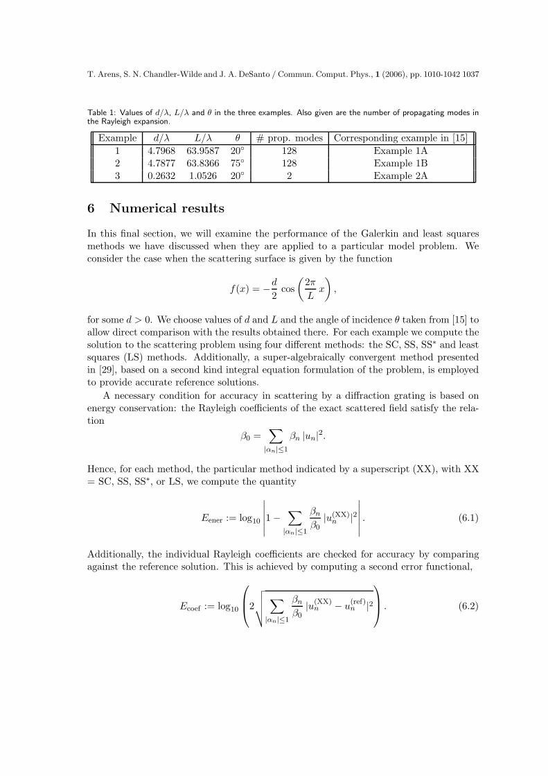
Table 1: Values of d/λ, L/λ and θ in the three examples. Also given are the number of propagating modes inthe Rayleigh expansion.

Example d/λ L/λ θ # prop. modes Corresponding example in [15]

1 4.7968 63.9587 20 128 Example 1A2 4.7877 63.8366 75 128 Example 1B3 0.2632 1.0526 20 2 Example 2A

6 Numerical results

In this final section, we will examine the performance of the Galerkin and least squaresmethods we have discussed when they are applied to a particular model problem. Weconsider the case when the scattering surface is given by the function

f(x) = −d

2cos

(

2π

Lx

)

,

for some d > 0. We choose values of d and L and the angle of incidence θ taken from [15] toallow direct comparison with the results obtained there. For each example we compute thesolution to the scattering problem using four different methods: the SC, SS, SS∗ and leastsquares (LS) methods. Additionally, a super-algebraically convergent method presentedin [29], based on a second kind integral equation formulation of the problem, is employedto provide accurate reference solutions.

A necessary condition for accuracy in scattering by a diffraction grating is based onenergy conservation: the Rayleigh coefficients of the exact scattered field satisfy the rela-tion

β0 =∑

|αn|≤1

βn |un|2.

Hence, for each method, the particular method indicated by a superscript (XX), with XX= SC, SS, SS∗, or LS, we compute the quantity

Eener := log10

∣

∣

∣

∣

∣

∣

1 −∑

|αn|≤1

βnβ0

|u(XX)n |2

∣

∣

∣

∣

∣

∣

. (6.1)

Additionally, the individual Rayleigh coefficients are checked for accuracy by comparingagainst the reference solution. This is achieved by computing a second error functional,

Ecoef := log10

2

√

√

√

√

∑

|αn|≤1

βnβ0

|u(XX)n − u

(ref)n |2

. (6.2)


The weights in this definition are selected to make the values of Eener and Ecoef comparable.In particular, using the discrete Holder inequality, we have that

1 −∑

|αn|≤1

βnβ0

|u(XX)n |2 =

∑

|αn|≤1

βnβ0

(

|un|2 − |u(XX)

n |2)

≤∑

|αn|≤1

βnβ0

|un − u(XX)n | |un + u(XX)

n |

≤

∑

|αn|≤1

βnβ0

|un + u(XX)n |2

1/2

∑

|αn|≤1

βnβ0

|un − u(XX)n |2

1/2

≤(

4 + 2 × 10Eener

)1/2

∑

|αn|≤1

βnβ0

|un − u(XX)n |2

1/2

.

Hence, we expect Eener ≤ Ecoef for any reasonably accurate numerical method.Table 1 gives the values of d, L (relative to the wavelength) and θ for the various

examples. In each case, the calculations were carried out for a number of spaces (XN , YN ),starting with the spaces corresponding to the propagating modes and then increasing Nby symmetrically adding evanescent modes. In the case of the SS, SS∗, and LS methods,the coefficients in the linear system matrix have to be computed by numerical quadrature.As suggested in Section 4 we use an M -point trapezoidal rule which is rapidly convergentas M increases, and select values for M which ensure that the integrals are computed tomachine accuracy.

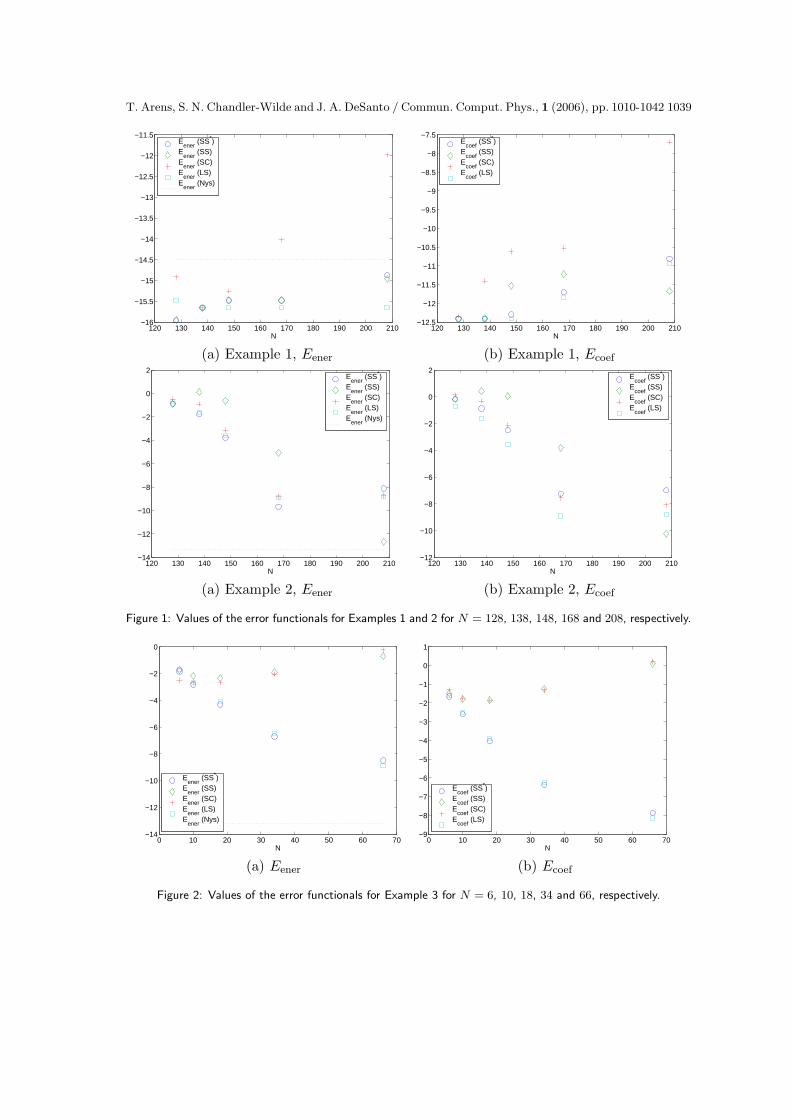
The computed values for the functionals Eener and Ecoef for Examples 1 and 2 aredisplayed in Fig. 1. For the near normal incidence of Example 1, all methods performequally well and compute the scattered field to high accuracy, even without any evanes-cent modes represented in the discrete spaces. Given that the total arc-length of Γ isapproximately 130λ, we see that all methods are very efficient, achieving close to machineaccuracy with N = 128, i.e. with less than one degree of freedom per wavelength of theboundary. For comparison, to achieve similar accuracy, the super-algebraically convergentNystrom method of [29] requires the solution of a linear system over 20 times larger. Whenthe number of unknowns is increased, the SC method shows some signs of instability. Itis worth noting that the functional Eener is rather smaller in this example than Ecoef , sothat Eener gives a somewhat misleading impression of the achieved accuracy.

In the case of the near grazing incidence of Example 2, the situation is somewhatdifferent: all methods require a substantial number of evanescent modes to be includedin the discrete spaces to compute the scattered field accurately. However, eventually allmethods do provide accurate results which is a new observation compared to [15] whereonly a few evanescent modes were used. We note, moreover, that even with the largestvalue of N used (N = 210) the number of degrees of freedom per wavelength is verymodest (≈ 1.6) given the high accuracy achieved.


120 130 140 150 160 170 180 190 200 210−16

−15.5

−15

−14.5

−14

−13.5

−13

−12.5

−12

−11.5

N

Eener

(SS*)E

ener (SS)

Eener

(SC)E

ener (LS)

Eener

(Nys)

120 130 140 150 160 170 180 190 200 210−12.5

−12

−11.5

−11

−10.5

−10

−9.5

−9

−8.5

−8

−7.5

N

Ecoef

(SS*)E

coef (SS)

Ecoef

(SC)E

coef (LS)

(a) Example 1, Eener (b) Example 1, Ecoef

120 130 140 150 160 170 180 190 200 210−14

−12

−10

−8

−6

−4

−2

0

2

N

Eener

(SS*)E

ener (SS)

Eener

(SC)E

ener (LS)

Eener

(Nys)

120 130 140 150 160 170 180 190 200 210−12

−10

−8

−6

−4

−2

0

2

N

Ecoef

(SS*)E

coef (SS)

Ecoef

(SC)E

coef (LS)

(a) Example 2, Eener (b) Example 2, Ecoef

Figure 1: Values of the error functionals for Examples 1 and 2 for N = 128, 138, 148, 168 and 208, respectively.

0 10 20 30 40 50 60 70−14

−12

−10

−8

−6

−4

−2

0

N

Eener

(SS*)E

ener (SS)

Eener

(SC)E

ener (LS)

Eener

(Nys)

0 10 20 30 40 50 60 70−9

−8

−7

−6

−5

−4

−3

−2

−1

0

1

N

Ecoef

(SS*)E

coef (SS)

Ecoef

(SC)E

coef (LS)

(a) Eener (b) Ecoef

Figure 2: Values of the error functionals for Example 3 for N = 6, 10, 18, 34 and 66, respectively.


Table 2: Values of log10

‖AN‖, log10

‖A−1

N‖, and est, the approximate upper bound on log

10‖A−1

N‖.

Example 1

N log10 ‖AN‖ log10 ‖A−1N ‖ est

128 0.44 0.42 0138 0.45 4.91 10.46148 0.45 8.82 15.13168 0.45 14.84 22.21208 0.45 16.89 33.50

Example 2


128 0.43 0.40 0138 0.44 4.85 10.35148 0.44 8.76 15.04168 0.44 14.83 22.13208 0.44 17.11 33.43

Example 3


6 0.08 1.30 3.3010 0.09 2.71 6.1718 0.09 5.57 11.7034 0.09 11.32 22.6666 0.09 17.51 44.52

The situation changes significantly in Example 3, as illustrated in Fig. 2. For thiscase the SS and SC methods do not give accurate results for any N , while the SS∗ andLS methods converge as N increases, at least up to N = 66. However, as predictedtheoretically, the condition numbers of the linear systems grow as N increases, reachingthe value 6.7 × 1017 for N = 66. This large value of the condition number appears to beslowing the convergence rate, so that the results for N = 66 are not as accurate as wouldbe expected from extrapolating the convergence rate from lower values of N . Nevertheless,the SS∗ and LS methods are pretty effective, achieving quite accurate results with N = 34,i.e. with ≈ 14 degrees of freedom per wavelength (Γ has arc-length ≈ 2.4λ).

The conditioning of the system matrices is studied in a little more detail in Table 2,where we tabulate the norm of AN and κ2

N = ‖A−1N ‖. The estimate (4.33) predicts that,

for every ǫ > 0, κ2N ≤ C exp(2k(d + ǫ)β∗N ), where the constant C depends only on ǫ, d,

L and k, and β∗N denotes the maximum value of ℑβn over the modes n included in theapproximation space. To give some indication of the numerical value of this estimate wehave tabulated log10(exp(2k dβ∗N )) ≈ 0.869 k dβ∗N in the column labelled est.

The results show that ‖A−1N ‖ and the condition number condAN = ‖AN‖ ‖A

−1N ‖ in-

crease rapidly as N increases, once the approximation space starts to contain evanescentmodes. Moreover, the principle of exponential growth of ‖A−1

N ‖, suggested by the bound(4.33), appears to be supported by our numerical results, though the bound overestimatesthe value of κN by orders of magnitude, in fact appears to overestimate the rate of expo-nential increase of ‖A−1

N ‖ by approximately a factor of two. We note that ‖AN‖ remainsbounded as N increases.


References

[1] H. Abe and T. Sato, Boundary integral equations from Hamilton’s principle for surfaceacoustic waves under periodic metal gratings, IEEE T. Ultrason. Ferr. Freq. Control, 47(2000), 1601–1603.

[2] G. Bao, D.C. Dobson and J.A. Cox, Mathematical studies in rigorous grating theory, J. Opt.Soc. Am. A, 12 (1995), 1029–1042.

[3] T. E. Betcke and L. N. Trefethen, Reviving the method of particular solutions, SIAM Rev.,47 (2005), 469–491.

[4] R. Brauer and O. Bryngdahl, Electromagnetic diffraction analysis of 2-dimensional gratings,Opt. Commun., 100 (1993), 1–5.

[5] O. P. Bruno and F. Reitich, Numerical solution of diffraction problems - a method of variationof boundaries. 2. Finitely conducting gratings, Pade approximants, and singularities, J. Opt.Soc. Am. A, 11 (1994), 2816–2828.

[6] M. Cadilhac, Some mathematical aspects of the grating theory, in: R. Petit (Ed.), Electro-magnetic Theory of Gratings, Springer-Verlag, Berlin, 1980, pp. 53–62.

[7] S. N. Chandler-Wilde, The impedance boundary value problem for the Helmholtz equationin a half-plane, Math. Meth. Appl. Sci., 20 (1997), 813–840.

[8] S. N. Chandler-Wilde and B. Zhang, Electromagnetic scattering by an inhomogenous con-ducting or dielectric layer on a perfectly conducting plate, Proc. R. Soc. Lon. A, 454 (1998),519–542.

[9] S. N. Chandler-Wilde and B. Zhang, A uniqueness result for scattering by infinite roughsurfaces, SIAM J. Appl. Math., 58 (1998), 1774–1790.

[10] D. Colton and R. Kress, Integral Equation Methods in Scattering Theory, Wiley, New York,1983.

[11] D. Colton and R. Kress, Inverse Acoustic and Electromagnetic Scattering Theory, Springer,Berlin, 1998, 2nd edition.

[12] J. A. DeSanto, Scattering from a perfectly reflecting arbitrary periodic surface: An exacttheory, Radio Sci., 16 (1981), 1315–1326.

[13] J. A. DeSanto, Exact spectral formalism for rough-surface scattering, J. Opt. Soc. Am., A2(1985), 2202–2207.

[14] J. A. DeSanto, Scattering from rough surfaces, in: R. Pike and P. Sabatier (Eds.), Scattering,Academic Press, 2002, pp. 15–36.

[15] J. A. DeSanto, G. Erdmann, W. Hereman and M. Misra, Theoretical and computational as-pects of scattering from rough surfaces: One-dimensional perfectly reflecting surfaces, WavesRandom Media, 8 (1998), 385–414.

[16] J. A. DeSanto, G. Erdmann, W. Hereman and M. Misra, Theoretical and computationalaspects of scattering from periodic surfaces: One-dimensional transmission interfaces, WavesRandom Media, 11 (2001), 425–453.

[17] J. Elschner and G. Schmidt, Diffraction in periodic structures and optimal design of binarygratings I: Direct problems and gradient formulas, Math. Meth. Appl. Sci., 21 (1998), 1297–1342.

[18] J. Elschner and M. Yamamoto, An inverse problem in periodic diffractive optics: reconstruc-tion of Lipschitz grating profiles, Appl. Anal., 81 (2002), 1307–1328.

[19] H. W. Engl, M. Hanke and A. Neubauer, Regularization of Inverse Problems, Kluwer, Dor-drecht, 1996.

[20] L. F. Li, Multilayer-coated diffraction gratings - differential equation method of Chandezon


et al revisited, J. Opt. Soc. Am. A, 11 (1994), 2816–2828.[21] L. F. Li, J. Chandezon, G. Granet and J. P. Plumey, Rigorous and efficient grating-analysis

method made easy for optical engineers, Appl. Optics, 38, 304–313 (1999).[22] A. Kirsch, Diffraction by periodic structures, in: L. Pavarinta and E. Somersalo (Eds.),

Inverse Problems in Mathematical Physics, Springer, Berlin, 1993, pp. 87–102.[23] A. Kirsch, Uniqueness theorems in inverse scattering theory for periodic structures, Inverse

Probl., 10 (1994), 145–152.[24] A. Kirsch, An Introduction to the Mathematical Theory of Inverse Problems, Springer, Berlin,

1996.[25] R. Kress, Numerical Analysis, Springer, Berlin, 1998.[26] R. Kress, Linear Integral Equations, Springer, Berlin, 1999, 2nd edition.[27] C. M. Linton, The Green’s function for the two-dimensional Helmholtz equation in periodic

domains, J. Eng. Math., 33 (1998), 377–402.[28] D. Maystre, Rigorous vector theories of diffraction gratings, in: E. Wolf (Ed.), Progress in

Optics XXI, Elsevier, Amsterdam, 1984, pp. 1–67.[29] A. Meier, T. Arens, S. N. Chandler-Wilde and A. Kirsch, A Nystrom method for a class of

integral equations on the real line with applications to scattering by diffraction gratings andrough surfaces, J. Integral Equations Appl., 12 (2000), 281–321.

[30] R. F. Millar, The Rayleigh hypothesis and a related least-squares solution to scattering prob-lems for periodic surfaces and other scatterers, Radio Sci., 8 (1973), 785–796.

[31] M. Neviere and E. Popov, Analysis of dielectric gratings of arbitrary profiles and thicknesses- comment, J. Opt. Soc. Am. A, 9 (1992), 2095–2096.

[32] M. Nieto-Vesperinas, Scattering and Diffraction in Physical Optics, Wiley, New York, 1991.[33] A. F. Peterson, An outward-looking differential equation formulation for scattering from one-

dimensional periodic diffraction gratings, Electromagnetics, 14 (1994), 227–238.[34] R. Petit (Ed.), Electromagnetic Theory of Gratings, Springer, Berlin, 1980.[35] A. Pomp, The integral method for coated gratings: Computational cost, J. Mod. Optics, 38

(1991), 109–120.[36] A. G. Voronovich, Wave Scattering from Rough Surfaces, Springer, Berlin, 1998, 2nd edition.

Documents

Preservation of Electronic Records Workshop