Presented to - Uniandes

DEGREE PROJECT

Presented to

LOS ANDES UNIVERSITYSCHOOL OF ENGINEERING

DEPARTMENT OF ELECTRICAL AND ELECTRONIC ENGINEERING

Project submitted for the degree of

ELECTRICAL ENGINEER

by

Ana Leonor Acevedo Perez

Economic Optimization of Insulation and Grounding in AC Transmission LineExposed to Direct Lightning Strokes

Thesis submitted on June 5, 2019 to:

- Advisor: Paulo Manuel de Oliveira de Jesus PhD, Associate Professor, Los Andes University

- Juror: Mario Alberto Rıos Mesıas PhD, Full Professor, Los Andes University

- Juror: Alvaro Torres Macıas PhD, Full Professor, Los Andes University

To all of you...

AcknowledgmentsI would like to express my gratitude to my advisor Paulo Manuel De Oliveira for his patience, moti-vation, explanations and time employed in this project. To my family for their unconditional supportduring my time at university. Finally, to all my friends, especially to Juan Camilo Amaya for sharingall his university life with me.

i

Contents

1 Introduction 2

2 State of the Art 32.1 Estimation of The Lightning Performance of Overhead

Transmission Lines . . . . . . . . . . . . . . . . . . . . . . . . . . . . . . . . . . . . . . . 32.2 Economic Perspective . . . . . . . . . . . . . . . . . . . . . . . . . . . . . . . . . . . . . 3

3 Methods to evaluate the Back Flashover Rate 53.1 EPRI Method . . . . . . . . . . . . . . . . . . . . . . . . . . . . . . . . . . . . . . . . . . 53.2 IEEE 1243 - Guide for Improving the Lightning Performance of Transmission Lines . . . 63.3 CIGRE - Guide to Procedures for Estimating the Lightning Performance of Transmission

Lines . . . . . . . . . . . . . . . . . . . . . . . . . . . . . . . . . . . . . . . . . . . . . . . 73.4 Montecarlo-ATP-EMTP method . . . . . . . . . . . . . . . . . . . . . . . . . . . . . . . 83.5 Methods comparison . . . . . . . . . . . . . . . . . . . . . . . . . . . . . . . . . . . . . . 8

4 The Optimization Model 114.1 The Back Flashover Rate parameterization [15] . . . . . . . . . . . . . . . . . . . . . . . 114.2 Economics of Mitigation of Back Flashover Phenomena [15] . . . . . . . . . . . . . . . . 12

4.2.1 Grounding Costs [15] . . . . . . . . . . . . . . . . . . . . . . . . . . . . . . . . . . 124.2.2 Additional Insulation Cost [15] . . . . . . . . . . . . . . . . . . . . . . . . . . . . 154.2.3 Optimization Model [15] . . . . . . . . . . . . . . . . . . . . . . . . . . . . . . . . 16

5 Case Study 185.1 EPRI-Transmission Line Reference Book . . . . . . . . . . . . . . . . . . . . . . . . . . . 185.2 Colectora 1 - Cuestecitas - La Loma Transmission Line . . . . . . . . . . . . . . . . . . . 19

6 Results 206.1 Back Fashover Rate BFR . . . . . . . . . . . . . . . . . . . . . . . . . . . . . . . . . . . 206.2 Optimization Problem - Transmission Line Reference Book . . . . . . . . . . . . . . . . 216.3 Optimization Problem: Colectora 1 - Cuestecitas - La Loma . . . . . . . . . . . . . . . . 24

6.3.1 Limitations . . . . . . . . . . . . . . . . . . . . . . . . . . . . . . . . . . . . . . . 266.4 Summary of results . . . . . . . . . . . . . . . . . . . . . . . . . . . . . . . . . . . . . . . 26

7 Conclusions 27

References 27

ii

List of Figures

3.1 Comparison between the first stroke lightning current distributions adopted by CIGREand IEEE . . . . . . . . . . . . . . . . . . . . . . . . . . . . . . . . . . . . . . . . . . . . 9

4.1 Transmission line definition with n sections . . . . . . . . . . . . . . . . . . . . . . . . . 114.2 Supplemental grounding electrodes with nr radial wires . . . . . . . . . . . . . . . . . . 134.3 Electrode cost CGk in function to steady state resistance R0 . . . . . . . . . . . . . . . . 14

5.1 Tower Sketch . . . . . . . . . . . . . . . . . . . . . . . . . . . . . . . . . . . . . . . . . . 185.2 Case study transmission line route . . . . . . . . . . . . . . . . . . . . . . . . . . . . . . 19

6.1 Resistivity profile . . . . . . . . . . . . . . . . . . . . . . . . . . . . . . . . . . . . . . . . 22

6.2 Total cost between range from 0.1 to 1.2outage

100km·yearfor EPRI transmission line . . . . . 23

6.3 Marginal cost between range from 0.1 to 1.2outage

100km·yearfor EPRI transmission line . . . 23

6.4 Total cost between range from 0.1 to 1.2outage

100km·yearfor colectora 1 - Cuestecitas trans-

mission line . . . . . . . . . . . . . . . . . . . . . . . . . . . . . . . . . . . . . . . . . . . 246.5 Marginal cost between range from 0.1 to 1.2

outage100km·year

for Colectora 1 - Cuestecitas

transmission line . . . . . . . . . . . . . . . . . . . . . . . . . . . . . . . . . . . . . . . . 25

iii

List of Tables

3.1 Parameters of the first stroke distributions adopted by CIGRE . . . . . . . . . . . . . . 73.2 Statistical parameters of first negative and positive return-strokes current . . . . . . . . 83.3 Flash collection rate to the transmission line . . . . . . . . . . . . . . . . . . . . . . . . . 9

5.1 Tower coordinates and radius conductors . . . . . . . . . . . . . . . . . . . . . . . . . . . 185.2 Transmission Line Description [1], [2] . . . . . . . . . . . . . . . . . . . . . . . . . . . . . 195.3 Case study tower coordinates and radius conductors . . . . . . . . . . . . . . . . . . . . 19

6.1 Number of flashes to line . . . . . . . . . . . . . . . . . . . . . . . . . . . . . . . . . . . . 206.2 Probability of BFR occurrence . . . . . . . . . . . . . . . . . . . . . . . . . . . . . . . . 206.3 Back flashover rate BFR . . . . . . . . . . . . . . . . . . . . . . . . . . . . . . . . . . . . 216.4 Back Flashover Parameterization Parameters αij . . . . . . . . . . . . . . . . . . . . . . 22

iv

AbstractThe reliability of an alternating current transmission line is strongly dependent of the occurrence ofdirect lightning strokes that terminates in a shield wire or a tower structure. This event could producea flash from the tower structure to any phase of the circuit when the insulation is not able to with-stand the overvoltage. This phenomenon is called Back Flashover and it can be statistically assessedby means of a Back Flashover Rate (BFR) expressed in flashes per year per line length. The reductionof the BFR -and therefore the reliability improvement- depends on the quality of the tower groundingand the number of insulators installed in the affected tower. This problem has been treated usingdifferent methods, from cookbook step-by-step procedures to Montecarlo-based techniques resortingadvanced electromagnetic simulation programs.

However, above-mentioned procedures do not take into account economic considerations. Under mod-ern performance-based regulation, transmission assets such as grounding electrodes and insulationsystems must be included in the base-rate as constructive elements attending economic efficiency.Thus, overinvestment on mitigation infrastructure should not be allowed. In 1967, Hileman [12] statedthat the mitigation infrastructure (grounding & insulation) could be specified according to a desirableBFR at minumum overall cost. Thus, total and marginal cost of additional insulation and groundingdevices can be evaluated for each BFR value. The economic optimization model suggested by Hilemanwas updated and generalized by De Oliveira in 2019 [15]. The methodology was updated accountingdynamic grounding behavior and illustrated with the well-known step-by-step Red Book EPRI modelto evaluate the desired BFR of a HVAC 345kV double circuit line (2005).

In this document, De Oliveira/Hileman [12,15] economic optimization model was applied in the sameEPRI’s 345kV HVAC line using four different BFR techniques such as EPRI Red Book, IEEE 1247(Flash program), CIGRE and Montecarlo-ATP. Resulting marginal and total cost curves of the BFRare evaluated and compared. Furthermore, the economic method was also applied to a real-worldtransmission line located in Colombia (Colectora 1 - Cuestecitas - La Loma 500kV). The method al-lows to determine marginal cost of the BFR either for the EPRI test case (345kV) or the Colombiantest case (500kV).

In the EPRI’s test case (HVAC 345kV line), results show that three methods (EPRI method, IEEEFlash and Montecarlo-ATP-EMTP) yield very similar total and marginal cost-BFR curves. The CI-GRE method yields a more optimistic curve (lower costs) when the desired BFR is low. The investmentcost in grounding and insulation to assure a BFR of 1 outage/100km/year is around US$2.5 million.

In the Colombian Case HVAC 500kV line, results show that CIGRE, EPRI method, IEEE Flash andMontecarlo-ATP-EMTP yield similar total and marginal cost-BFR curves. The most conservativeresult (higher costs) is the IEEE Flash method and the most optimistic one is EPRI (lower costs).The investment cost in grounding and insulation to assure a BFR of 1 outage/100km/year is aroundUS$5 million (EPRI) - US$8 million (IEEE Flash).

1

1. IntroductionOvervoltages due to lightning strokes are one of the main causes of faults in power systems. Whenlightning strikes the tower or ground wires, the current on the tower and ground impedances cause therise of tower voltage. Thus, the tower and shield wires voltage becomes much larger than the phaseconductors voltages. If that voltage difference exceeds a critical value of specified insulation level, aflashover occurs called back flashover BF, and the corresponding minimum lightning current that pro-duces it is called critical current. Followed this, it is produced a short circuit phase-earth where surgeprotection acts and generate the outage line. Consequently, the back flashover rate (BFR) determinethe performance of transmission lines due to direct lightning and it is one of the main methods tocompute transmission line reliability indexes [15].

Lightning protection system LPS allows reducing the BF phenomenon. These encompass the spec-ification of insulation levels, supplemental grounding electrodes, the installation of additional shieldwires and line arresters. Besides, designers tend to specify supplemental grounding electrodes as themain mitigation measure to reduce back flashover rate.

The reduction of the BFR -and therefore the reliability improvement- depends on the quality of thetower grounding and the number of insulators installed in the affected tower. This problem has beentreated using different methods, from cookbook step-by-step procedures to Montecarlo-based tech-niques resorting advanced electromagnetic simulation programs.

However, above-mentioned simulation methods do not take into account economic considerations.Under modern performance-based regulation, transmission assets such as grounding electrodes andinsulation systems must be included in the base-rate as constructive elements attending economic ef-ficiency. Thus, overinvestment on mitigation infrastructure should not be allowed.

In 1967, Grosser & Hileman [12] stated that the mitigation infrastructure (grounding & insulation)could be specified according to a desirable BFR at minumum overall cost. Thus, total and marginalcost of additional insulation and grounding devices can be evaluated for each BFR value. The economicoptimization model suggested by Hileman was updated and generalized by De Oliveira in 2019 [6]. Themethodology accounts the dynamic grounding behavior and it is illustrated with the well-known step-by-step Red Book EPRI model to evaluate the desired BFR of a HVAC 345kV double circuit line (1982).

In this document, as main contribution the De Oliveira’s economic optimization model was appliedin the same EPRI’s 345kV HVAC test line using other different BFR techniques such as IEEE 1247(Flash program), CIGRE and Montecarlo-ATP-EMTP for comparison purposes. Resulting marginaland total cost curves of the BFR are evaluated and discussed. Furthermore, the economic method wasalso applied to a real-world transmission line located in Colombia (Colectora 1 - Cuestecitas - La Loma500kV) specified in the Colombian reference expansion plan 2017-2031 defined by UPME (ColombianEnergy Mining Panning Unit) [23].

This thesis is organized as follows. In chapter 2, State of art on BFR evaluation methods from technicaland economical perspective are presented. Chapter 3 develops the theoretical framework of the thesis.EPRI, IEEE 1243, CIGRE and Montecarlo-ATP-EMTP approaches are described. The optimizationmodel is described in Chapter 4. The case studies are defined in Chapter 5. Results are discussed inChapter 6 and conclusions are drawn in Chapter 7.

2

2.State of the Art

2.1 Estimation of The Lightning Performance of OverheadTransmission Lines

There are different deterministic and probabilistic methods to determine outage rate due to backflashover. In first place, Transmission Line Reference Book [9] presents a step by step two pointmethod to compute lightning performance of transmission lines. This deterministic method, assumesthe transmission line as a uniform stretch, without taking into account the variations in the resistivityof the terrain and keraunic level. Although two point method has limitations, it is still widely used inthe industry.

Moreover, Nucci [18] presents a survey on CIGRE [4] and IEEE [14] procedures for the estimation ofthe lightning performance. The conclusion of this paper is the main differences lie in the fact that somemethods proposed so far within CIGRE can be considered to be more general than those proposedwithin IEEE, in that they take into account more variables of the problem. The relevant drawback isthat no software tool has been made freely available so far within CIGRE, while within IEEE - thanksin part to the inherent simpler approach - some computer code, such as Flash [14], has been madeavailable.

Finally, probabilistic methods consist on the implementation of a Monte Carlo procedure to evaluatethe BFR of a given overhead line [10]. In order to get more precision, the authors developed a fullstatistical procedure. Monte Carlo procedure generates a large population of N lightnings, assumedto fall within a 1 km-wide swath centered on the overhead transmission line: among these, the largesample of NL flashes that actually hit the line is extracted by means of an electrogeometric model andthe attendant strokes are simulated by the ATP-EMTP system model, including statistical modelingof line insulation breakdown, yielding Ndisc total flashovers out of N strokes.

2.2 Economic Perspective

It is important to mention that there are not many articles and researches about the relationship be-tween outage rates and the required investment costs to reduce it. In the last sixties [12] presented thefirst economic approach to evaluate the reliability of transmission systems exposed to direct lightningstrokes and back-flashover phenomena. As well, recently [15] presents a unified economic approach toevaluate the reliability of transmission systems exposed to direct lightning strokes and back flashoverphenomena.

In 1967, George E. Grosser and Andrew R. Hileman [12] presented a mathematical model relating toline performance. Thus, analyze insulation system expenditure and proposed a method for optimizingthe selection of insulation system components aim to achieve a desired performance or reliability level,using incremental cost techniques. The development provides an insight into the interaction of towergrounding and tower insulation in establishing the reliability of a line.

Customarily, the balance between the use of additional insulation and supplementary grounding toobtain a specific line flashover performance is achieved assuming that the tower insulation and thetower footing resistance selected to apply for the entire line. Tower design economics usually dictateagainst tower insulation variations along the line because of mechanical considerations provide a basisfor maintaining the number of insulators and the coordinated tower clearances constant.

Additionally, [12] mention that tower footing resistance only affects the lightning flashover rate. Fur-ther, lightning strokes terminating on the ground wire system normally produce high overvoltagesacross the insulation at only one or two adjacent towers. This localized nature of lightning produced

3

CHAPTER 2. STATE OF THE ART 4

voltages along with the freedom in the grounding selection suggest that tower grounding economicsshould be analyzed on an individual tower basis.

Finally, by mean of the Lagrangian multiplier theory, an incremental cost method was developed todetermine the economic optimum combination of tower insulation and supplemental tower groundingfor a prescribed degree of line reliability. The supplemental tower grounding is allocated on an indi-vidual tower basis so that the amount of supplemental grounding varies with soil resistivity, and spanlength associated with each tower.

Therefore, as a fundamental contribution, they stated that the cost of grounding and insulation asso-ciated to a prescribed BFR can be optimized. Hence, for each reliability level, there is an incrementalcost for the mitigation measures associated to a desirable outage rate.

On the other hand, De Oliveira De Jesus [15] investigates the relationship between the cost associatedwith lightning protection systems (LPS) and the back flashover rate (BFR) in high voltage trans-mission lines. The fundamental research question raised is how to determine the incremental cost ofthe mitigation measures (LPS) associated with a prescribed back flashover rate. The interaction oftower supplemental grounding and tower insulation design is analyzed satisfying a given reliabilitylevel at minimum overall investment cost. Besides, a new optimization model relating back flashoverphenomena to expenditure in LPS is presented expressly accounting the dynamic behavior of thetower footings being suitable to be applied using step-by-step Anderson EPRI method BFR evaluationmethodology [9].

3.Methods to evaluate the Back Flashover RateIn this section, four methods to evaluate back flashover rates are described and compared. The first oneis the two-point method proposed in EPRI Red Book [9]. The second one is the method implementedin the IEEE Guide for Improving the Lightning Performance of Transmission Lines [14]. The thirdmethod is implemented in CIGRE - Guide to the procedure for estimating the lightning performance ontransmission lines [4]. Finally, the last one method is Monte Carlo method for estimating backflashoverrates [21].

3.1 EPRI Method

According to [9], to determine the lightning performance it is necessary the knowledge of the lightningactivity (flashes to earth per square kilometer per year) η. If a measured value of ground flash densityis not available, it may be estimated based on keraunic level T, in thunders-days per year in the area.

η = 0.12 · T[

flashes

km2 · year

](3.1)

On top of that, a transmission line passing above the earth throw an electrical shadow on the landbeneath. Lightning flashes that would generally terminate on the land inside the shadow will strikethe line instead, whereas flashes outside this shadow will miss the line entirely. Thus, the relationshipbetween the number of flashes to the line becomes:

µ = η

(b+ 4 · h1.09g

10

) [Lines-flashes

100km · year

](3.2)

Where µ is the number of flashes to the line per 100 km per year, hg is tower height and b is the linewidth. Concerning the lightning exposure, the next step is simplified models capable of estimating thelightning strike incidence to transmission lines, to provide suitable engineering procedures to evaluateboth incidence of lightning strikes and optimal position of shielding wires. The model applied to cal-culate lightning incidence on transmission lines is the conventional electrogeometric model EGM.

The basic concept of the EMG is that takes into account the downward lightning leader only, withouttaking into consideration the upward (positive) leader from the structure. It assumes that the leaderchannel is perpendicular to the ground plane and that the flash will stroke the tower if its prospectiveground termination point lies within the attractive radius r. The attractive radius depends on severalfactors, such as the charge of the leader, its distance from the structure, type of structure (a verticalmast or horizontal conductor), structure height and nature of the terrain.

Also, the downward motion of a lightning leader approaching ground is assumed to continue unper-turbed unless critical field conditions develop allowing a juncture with a nearby vertical object generallycalled final jump [14].

Furthermore, the lightning statistical log-normal curve is approximated with a quite reasonable accu-racy between 2 kA and 200 kA with Popolansky curve [9]. The cumulative probability of If exceedingI [kA] is:

P (If > I) =1

1 +(

I31 kA

)2.6 (3.3)

2 kA < I < 200 kA

5

CHAPTER 3. METHODS TO EVALUATE THE BACK FLASHOVER RATE 6

Thus, the BFR is given by the probability of exceeding the critical current multiplied by the numberof flashes to the shield wires, µ:

BFR = 0.6 ·NL · PI (I > Ic) (3.4)

3.2 IEEE 1243 - Guide for Improving the Lightning Performance ofTransmission Lines

In this case, the ground flash density η may be estimated using:

η = 0.04 · T 1.25d

flashes

km2 · year(3.5)

Where Td is the keraunic level (number of thunderstorm-days per year). The flash collection rate µ,is given by the following equation:

µ = η

(28 · h0.6 + b

10

)flashes

100km · year(3.6)

Where h is tower height and b is tower width. When lightning strikes a phase conductor, no otherobject shares in carrying the lightning current. Most flashes to an unprotected phase conductor aretherefore capable of producing flashovers. Ground wires may intercept the stroke and shunt the currentto the ground through the tower impedance and footing resistance if they are properly located. Theresultant voltages across the transmission-line insulation and the likelihood of flashover are substan-tially reduced [14].

The cumulative probability of If exceeding I [kA] is:

P (If > I) =1

1 +(

I31 kA

)2.6 (3.7)

2 kA < I < 200 kA

The lightning performance of an entire transmission line is influenced by the individual performanceof each tower and the performance of a tower with the average tower-footing impedance. In areasof nonhomogeneous earth resistivity, even a few towers located in high-resistivity soil may degradeline performance. When spotting towers, every attempt should be made to locate each one where thelocal resistivity is low. When this may not be done, line performance computations should be madeseparately for each significant class of tower footing impedance encountered.

The results may then be combined to determine the composite performance by the equation:

T =

∑TnLn∑Ln

(3.8)

Where T is the total outage rate, Ln is the length of line section n with homogeneous resistance andTn is the outage rate computed for line section n.


3.3 CIGRE - Guide to Procedures for Estimating the Lightning Per-formance of Transmission Lines

The ground flash density η is calculate by:

η = 0.04 · T 1.25 (3.9)

In the same way, the relationship between Ng and the number of flashes to the line becomes:

µ = η ·

[2 ·(14h0.6

)+ b

1000· 100km

](3.10)

The frequency distribution of first return-stroke lightning current peaks adopted by CIGRE [4] hasbeen derived from the available measurements of 338 negative downward flashes, collected in severalparts of the world on various structures (76 flashes on lines and 262 on masts and chimneys) of differentheights, in general, less than about 60 m. One-hundred twenty-five measurements are taken from thoserecorded at the Berger’s tower [18]. The cumulative distribution of these peak current peaks has amedian value of about 34 kA. The lightning current distribution by a lognormal one with the followingmedian and logarithmic standard deviation µI = 31.1kA, σI = 0.484:

f (I) =1√

2πσII· e−

(ln

(IµI

))2σ2I (3.11)

As noted by Anderson and Eriksson [4], such a lognormal distribution can be better represented by twosub-distributions that divide, in a first approximation, the shielding failure and back flashover domains.Table 3.1 reports the median and the logarithmic standard deviation of these two sub-distributions.

Table 3.1: Parameters of the first stroke distributions adopted by CIGRE

ParameterShielding Failure DomaninI < 20kA

back flashover DomainI > 20kA

µI 61 kA 33.3 kAσI 1.33 0.605

Since the crest voltage and the flashover voltage are both functions of the time-to-crest tf of thelightning current, the critical current previously determined is variable. Therefore, the BFR consideringall the possible time-to-crest values is:

BFR = 0.6 ·NL∫ ∞0

∫ ∞Ic(tf )

f

(I

If

)· f (tf ) dIdtf (3.12)

Where f(IIf

)is the conditional probability density function of the stroke current given the time-

to-crest and f (tf ) is the probability function of the time-to-crest value. Another, more simplifiedprocedure for the calculation of the BFR, is also illustrated in [4] as the BFR resulting from the ap-plication of Eq. 3.12 can be obtained by using of an equivalent time-to-crest value Te. Such a valueis approximately the median value of time to crest for the specific critical current [18]. With such avalue, since a single equivalent front is used, the BFR is reduced to:


BFR = 0.6 ·NL∫ ∞IC

f (I) dI = 0.6 ·NL · P (I > IC) (3.13)

3.4 Montecarlo-ATP-EMTP method

Monte Carlo procedure generates a large population of N lightnings, assumed to fall within a 1 km-wideswath centered on the overhead transmission line: among these, the large sample of NL flashes thatactually hit the line is extracted by means of an electrogeometric model and the attendant strokes aresimulated by the ATP-EMTP system model, including statistical modeling of line insulation break-down, yielding Ndisc total flashovers out of N strokes.

BFR = 0.6 · NdiscN·Ng · 100 (3.14)

where the numerical multiplicative coefficient 0.6 accounts for the strokes terminating within the span

and Ng is the ground flash density flasheskm2·year .

Besides, the statistical variation of lightning stroke parameters (peak current Ip, front time tF and tailtime tT ) has been assumed to follow a log-normal distribution, with probability density function:

p (x) =1√

2 · πxσln x· exp

[−1

2

(lnx− lnxm

σln x

)2]

(3.15)

Where σln x is the standard deviation of lnx and xm is the median value of x [10]. Values of xm andσln x are:

Table 3.2: Statistical parameters of first negative and positive return-strokes current

Parameter Median Value Standart DeviationIp 35 kA 1.21tf 22 µs 1.23tT 230 µs 1.33

3.5 Methods comparison

This section presents a comparison between the methods described above, aiming to determine themain differences and from technical perspective.

First, EPRI red book method presents approximations and assumptions that generate important im-precision. Besides, IEEE [14] and CIGRE [4] methods, published by two of the world’s most author-itative scientific technical institutions in the area of the lightning performance of transmission lines,are accuracy and the results of back flashover rate are widely accepted.

Second, for all methods mentioned above, the amount of effective atmospheric discharges is equivalentto 60% of the atmospheric discharges that impact the transmission line. Third, for the problem of in-terest, the approaches proposed in the two frameworks (IEEE-CIGRE) are somewhat equivalent. Themain differences, when present, lie in the fact that some approaches proposed so far within CIGREcan be considered to be more general than those proposed within IEEE, in that they take into account


more variables of the problem. The relevant drawback is that no software tool has been made freelyavailable so far within CIGRE, while within IEEE - thanks in part to the inherent simpler approach- some computer code, such as Flash v.19 [14], has been made available, which can serve either asprofessional tools capable of providing a first approximate, yet extremely useful, answer on the light-ning performance of typical overhead transmission lines or as reference for beginner researchers whensimple cases are dealt with [18].

Table 3.3 shows the model adopted for each method to compute the flash collection rate to the trans-mission line.

Table 3.3: Flash collection rate to the transmission line

Method Assumption model Equation

EPRI Electrical shadow 0.1 · η(b+ 4 · h1.09g

) [ line-flashes100km·year

]IEEE 1243 Electrical shadow 0.1 · η

(b+ 28 · h0.6


]CIGRE Electrical shadow 0.1 · η

(b+ 28 · h0.6


]Monte-Carlo Electrogeometric model -

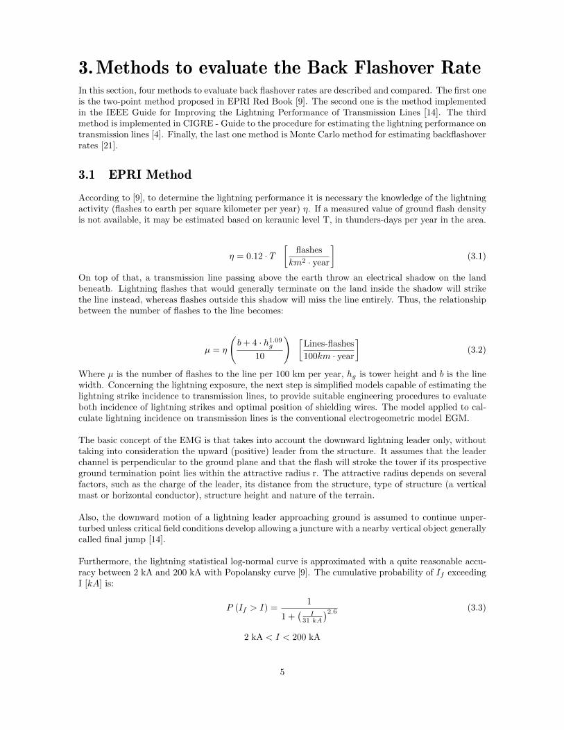
Likewise, the Figure 3.1 show the comparison between probability distribution curve for each deter-ministic method above mentioned. In the same way, Monte-Carlo method the probability of BFRoccurrence is calculated from the ratio between the number of downloads that caused back flashoverand the total number of simulated downloads.

20 40 60 80 100 120 140 160 180 200

current [kA]

0

0.005

0.01

0.015

0.02

0.025

pro

babili

ty

CIGRE

IEEE-EPRI

Figure 3.1: Comparison between the first stroke lightning current distributions adopted by CIGREand IEEE

Regarding tower voltage (an important aspect to computing BFR), EPRI, IEEE and CIGRE meth-ods are computed based on traveling waves model in equivalent model tower circuit, shield wires,


grounding, and nearby towers. Lightning current is a ramp waveform with wavefront at 2µs and 1 kAamplitude. Although, CIGRE method presents a variation in the way that wavefront varies from 1.2µsand 2µs, depending on minimum critical current. On the contrary, Monte Carlo method computestower voltage according to ATP simulations results and the lightning current is a ramp waveform whichamplitude is determined based on lognormal probability distribution with mean 33.3 kA and standarddeviation 6.605 and wavefront have a lognormal probability distribution with mean 2µs and standarddeviation 0.494.

Finally, the critical flashover voltage corresponds to the voltage-time curve of the insulator that de-pends on the insulation length. Thus, the minimum critical current is computed as a ratio betweenCFO and insulator voltage. EPRI method computes minimum critical current for 2µs and 6µs. In thesame way, IEEE estimated it for 2µs and 6µs in span distance less than 270 m and the calculationis made before the reflections of the other towers and at 6µs. In the case of CIGRE method, theminimum critical current is computed at wavefront time.

4.The Optimization ModelThis project is aiming to get Hileman & Grosser curves which using incremental cost techniquespresent a method for optimizing the selection of insulation system components to achieve a desiredperformance or reliability level [12]. The first one corresponds to the total cost curve in functionon the back flashover rate. The second curve is the relationship between marginal cost and backflashover rate. These curves are obtained as a result of the development of the method proposed byDe Oliveira [15]. In the first place, a prescribed back flashover rate is calculated and parameterized forthe four methods described in the above section. Then, an optimization problem is implemented todetermine the combination of additional grounding and insulation that minimizes infrastructure totalcost.

4.1 The Back Flashover Rate parameterization [15]

According to IEEE Std. 1243-1997 [14], the overall back-flashover rate of the line T, could be computedseparately for each tower or section k with similar resistivity and flash density characteristics. Thus,the sum of the specific outage rates per section k, Tk, determine the composite performance by thefollowing equation:

T =

n∑k=1

TkLkLT

outage

100 km · year(4.1)

In this way, to apply Eq. 4.1 transmission line is defined with length LT [km] and n sections ofLk [km]. Each line section k encompasses a number of towers Nk with similar geometry sketch, flashdensity ηk (flashes cloud-to-ground per km2-yr), earth resistivity ρk [Ω ·m] footing impedance Rbk [Ω]and number of insulators with insulator width ωbk [m] [15]. This definition is described in Figure 4.1.Besides, resistivity profile of the line is in general a known parameter and lightning parameters associ-ated with each section or tower are now available from detectors. Thus, procedures for back flashoverrate calculation should be applied separately for each section or tower.

Figure 4.1: Transmission line definition with n sections

The back flashover rate for each section k, Tk inoutage

100km·yearand the number of flashes that might strike

the tower (any phase or any overhead ground wire per 100 km per year) µk is calculated dependingon each method described in the last section.

Similarly, the probability function of a lightning current amplitude distribution Ik that will exceedthe critical current Ick required to produce back flashover is calculated according to each method forthe calculation of back flashover rate. Finally, the relationship between back flashover rate BFR anda number of variable of interest such as ηk, ρk, ωk and Rk can be parameterizer from the set of the

11

CHAPTER 4. THE OPTIMIZATION MODEL 12

solutions. Therefore, the control variables of the optimization problem are the impulse groundingimpedances Rk and the insulation length ωk, while environmental variables ηk is know in each sectionof transmission line. Hence, the parametric BFR function is given by the equation:

Tk = f (ηk, ωk, Rk) =

m∑i=1

m∑j=1

αijkηkωikR

jk (4.2)

Where, m is the fitting polynomial order, αijk ∀ i, j = 1, · · · ,m, k = 1, · · · , n are fitting parameters.In addition, Eq. 4.2 is Smooth and continuous. Thus, the first derivative are also continuous over therange under consideration in the parameterization process. As a result, the incremental flashover rateof the transmission line ∂Tk

∂Rkwith respect to the impulse grounding impedance Rk and the insulation

level ∂Tk∂ωk

will be necessary later to solve the optimization problem and can be written as:

∂Tk∂Rk

=

m∑i=0

m∑j=1

jαijkηkωikR

j−1k (4.3)

∂Tk∂ωk

=

m∑i=1

m∑j=0

iαijkηkωi−1k Rjk (4.4)

4.2 Economics of Mitigation of Back Flashover Phenomena [15]

The design of a transmission line should take into account some predefined basic factors such as theoperating voltage level, number of circuits, the route of the transmission line and the desired currentcapacity of the line. The amount and type of insulation generally is also determined by requirementsset forth by power frequency voltages and contamination and switching overvoltages. Besides, addi-tional redundancy and investments are required to ensure system security against lightning activityand back flashover phenomena.

Despite the construction costs of the line are significantly higher than the mitigation infrastructurerequired to reduce the back-flash rate, the designer should balance the costs of higher insulation levelsand improved grounding against the benefits of improved reliability. The trade-off between addinginsulation and improve grounding should be tackled from an economic viewpoint. Below, groundingand insulation costs are defined [15].

4.2.1 Grounding Costs [15]

Economic model required to evaluate grounding expenditure in the context of back flashover cost effec-tive design, the steady state grounding resistance and detailed dynamic model for grounding electroderesistances.

In the first place, each section k must be provided of a grounding means able to divert any lightningcurrent and short-circuit currents into earth. In the instance of high soil resistivity, self-resistance oftower footing is significantly high and supplemental ground electrodes should be added to the towerfootings. Defining Rbk and Rek as the power-frequency self-resistance and supplemental electrode re-sistance of section k, respectively. Then, the power-frequency grounding resistance can be defined asa function of natural and artificial resistance. What is more, when Rbk >> Rek, the effective towergrounding R0

k is equivalent to supplemental electrode resistance Rek.


There are different types of supplemental grounding electrodes with different geometries. For seek ofsimplicity, a single, two, three, four and eight-star horizontal radial wires nr of length lk [m] as showin Figure 4.2 are considered to illustrate the optimization methodology.

Figure 4.2: Supplemental grounding electrodes with nr radial wires

The power-frequency resistance of the supplemental electrode is computed according to the Sunde’sequations [15]:

Rek =ρk

nr · π · lk

ln

(2lkrg

)− 1 +

nr−1∑k=1

ln

1 + sin(πknr

)sin(πknr

) (4.5)

Where ρk is the single layer earth resistivity [Ω ·m] at section k, and nr is the number of horizontalradial wires. Then, assuming natural footing resistance Rbk greater than supplemental electrode resis-tance Rek, the corresponding power frequency grounding resistance at section k is giving by:

R0k = Rbk||Rek ≈ Rek (4.6)

On the other hand, the expenditure required for installing supplemental electrodes is a linear functionof the number of radial wires connected to the tower, the earth conductor length, exothermic connec-tions, excavation and backfilling. Contractors might settle different price points for soft soil and hardsoil due to the labor that it will take. Some soils are different to excavate than others. Excavationtasks can be manual or mechanical. Manual excavation technique is suitable for soft soils. Mechanicalexcavation technique is suitable for hard soils and subject to the access of the required machinery atthe working site. The total installation cost function of a supplemental electrode at section k is thenexpressed as [15]:

CGk = nrNklk (kesgd+ kc) (4.7)

Where Nk is the number of tower per section k, nr the numbers of radial wires with length lk, thetrench width sg and depth d. ke is the cost associated with manual or mechanical excavation, backfill-ing and compaction US$ per km3 and kc is the ground conductor cost US$ per m. Figure 4.3 showsthe electrode cost associate to steady state resistance R0 for nr horizontal radial wires.


0 10 20 30 40 50 60 70 80 90 100

R0 [ ]

0

2000

4000

6000

8000

10000

12000

CG

k[$

]

nr = 2

nr = 3

nr = 4

nr = 5

nr = 6

nr = 7

nr = 8

Figure 4.3: Electrode cost CGk in function to steady state resistance R0

Combining Eq. 4.6 and Eq. 4.7, the total cost of the grounding electrodes can be parameterized asfunction of the resistance R0

k and resistivity ρk as:

CGk = f(R0k, ρk

)= β

(ρkR0k

)γ(4.8)

0 ≤ R0k ≤ Rbk

γ > 1

Where β, γ are fitting parameters, Rk0 is the power frequency tower grounding resistance, and Rbk isthe natural tower grounding resistance. Also, the incremental cost of the steady-state resistance canbe derived of Eq. 4.8:

∂CGk∂R0

k

=−γβργk(R0

k)γ+1 (4.9)

In second place, an appropriate dynamic model for the tower grounding footing is crucial to assess theover voltages across the insulation strings when the lightning stroke impacts the tower or the shieldwires. Hence, the influence of the surge footing impedance on the tower top voltage is dependent onthe lightning current magnitude and the crest time. Thus, the dynamic grounding impulse resistanceassociated with concentrated supplemental electrode is expressed as:

Rk =R0k√

1 +2πIckR2

0

G0ρ

(4.10)

Where Ick (Rk, ωk) [kA] is the current magnitude of the lightning flash, R0k [Ω] is the power frequency

resistance and G0 [kVm ] is earth ionization electric field gradient and ρk [Ω ·m] is the earth resistivity.


Furthermore, Eq. 4.8 can be expressed as function of impulse resistance:

CGK (Rk, ωk) = Nkβ

(ρk

R0k (Rk)

)γ(4.11)

0 ≤ R0k (Rk) ≤ Rbk

γ > 1

Where,

R0k (Rk) =

√ρkG0Rk

ρkG0 + 2πIck (Rk, ωk) (Rk)2 (4.12)

Note that the grounding cost function not only depends on impulse resistance magnitude but alsodepends on the specified insulation length. Eq. 4.11 give us a specific formulation of the relationsamong electrode cost, impulse resistance and insulation level. Eq. 4.9 can be rewritten in order to getthe corresponding incremental costs of the grounding system. Thus, Eq. 4.13 and Eq. 4.14 expressthe incremental grounding costs ∂CGk

∂Rkand ∂CGk

∂ωk, respectively.

∂CGk∂Rk

= −

NkG0βγρkRk

ρ( G0ρkR2k

G0ρk−62πR2k

(3µk−5Tk

5Tk

) 513

)− 12

γ (13G0ρkT2k

(3µk−5Tk

5Tk

) 813 − 93πµk

∂Tk∂Rk

R3k

)

13T 2k

[G0ρk − 62πR2

k

(3µk−5Tk

5Tk

) 513

]2 (3µk−5Tk

5Tk

) 813

(G0R2

kρk

G0ρk−62πR2k

(3µk−5Tk

5Tk

) 513

)(4.13)

∂CGk∂ωK

=

93G0µkNkR4kβγρkπ

∂Tk∂Rk

ρk( G0R2kρk

G0ρk−62R2kπ

(3µk−5Tk

5Tk

) 513

)− 12

γ

13T 2k

[G0ρk − 62πR2

k

(3µk−5Tk

5Tk

) 513

]2 (3µk−5Tk

5Tk

) 813

(G0R2

kρk

G0ρk−62πR2k

(3µk−5Tk

5Tk

) 513

) (4.14)

Eq. 4.13 and Eq. 4.14 depend on the specified back flashover rate Tk given in Eq. 4.2, as well as itsfirst derivatives ∂Tk

∂Rkand ∂Tk

∂ωkdescribed in Eq. 4.3 and Eq. 4.4.

4.2.2 Additional Insulation Cost [15]

Adding more insulators in each phase of the transmission line to reduce the back-flashover rate impliesto modify the geometry of the tower. As a result, higher towers will require more steel to withstandtransversal external loadings [15]. A general formula to determine the tower weight WT [kg] neededto withstand external forces is:

WT = 1.9 · km ·

(∑g

hgtg +∑p

hptp

)(4.15)


Where km is 0.014 for double circuit lattice EHV systems, 0.021 for single circuit horizontal EHV sys-tems. hg is the height of each ground wire, hp is the height of each phase conductor of the tower, andtg and tp are the individual transverse force [kg] located at attachment height hg and hp, respectively.Then, when the insulator length in all phases varies, the additional weight of the tower ∆WT shouldbe recalculated accounting the displacements in all conductors.

Assuming a tower steel cost kt in US$kg and the factor σ0

k to account indirect costs, the incremental cost

of insulation σk

[US$kg

], at section k is:

σk =kt∆WT

0.146+ σ0

k ≈∂Cik∂ωk

(4.16)

Then, the total insulation cost in US $ for a section k with Nk towers is giving by:

CIk =

∫ ωk

ωbk

Nkσkdωk = Nkσk(ω − ωbk

)(4.17)

ωbk ≤ ωk ≤ ωmaxk

Where ωk [m] is the additional insulator length in all phases at section k and ωbk [m] is the basicinsulator length for switching surges (60 Hz) at section k.

4.2.3 Optimization Model [15]

The optimization problem find the set of impulse resistance, R = R1, · · · , Rk, · · · , Rn and the setof insulation length ω = ω1, · · · , ωn such that minimize the total investment costs in supplementarygrounding electrodes CG and tower insulation, defined in Eq. 4.11 and Eq. 4.17, subject to a pre-scribed global outage rate T ∗ described in Eq. 4.2 [15].

min ω,R

n∑k=1

Nkβ

[ρkR0k

]γ+Nkσk

(ωk − ωbk

)(4.18)

Subject to:

T ∗ =

n∑k=1

TkLkLT

ωbk ≤ ω ≤ ωmaxk ∀ k = 1, · · · , n

0 ≤ Rk ≤ Rbk ∀ k = 1, · · · , n

Where:

Tk =

m∑i=1

m∑j=1

αijkηkωikR

jk

The objective function and its first and second derivatives are continuous over the range under con-sideration. As the lowest investment cost in grounding and insulation is desired for achieving the


prescribed line performance, the problem can be interpreted as one of finding the minimum point onthe overall cost function under the restriction that the sum of the individual section performancesequal the desired line performance T ∗ [15].

Given the mathematical properties which have been attributed to the grounding and insulation costfunctions, this problem is suited to a solution employing Lagrangian multiplier theory which makespossible a straightforward mathematical approach to solving for the extremum of a continuous functionwhen restrictions are imposed. The Lagrangian function is given by:

L =

n∑k=1

CGk +

n∑k=1

CIk + λ

(n∑k=1

TkLkLT− T ∗

)+

n∑k=1

µ1k [ωkωmaxk ] +

n∑k=1

ν1k[ωbk − ωk

]· · · (4.19)

· · ·+n∑k=1

µ2k

[Rk −R0

k

]+

n∑k=1

ν2k [−Rk]

The first order conditions are given by:

∂L

∂ωk=∂CGk∂ωk

+∂CIk∂ωk

+ λLkLT

∂Tk∂ωk

+ µ1k − ν1k = 0 (4.20)

∂L

∂Rk=∂CGk∂Rk

+ λLkLT

∂Tk∂Rk

+ µ2k − ν2k = 0 (4.21)

∂L

∂λ=

n∑k=1

TkLkLT− T ∗ (4.22)

∂L

∂µ1k= ωk − ωmaxk ≤ 0, µ1k (ωk − ωmaxk ) = 0 (4.23)

∂L

∂ν1k= ωbk − ωk ≤ 0, ν1k

(ωbk − ωk

)= 0 (4.24)

∂L

∂µ2k= Rk −R0

k ≤ 0, µ2k

(Rk −R0

k

)= 0 (4.25)

∂L

∂ν2k= −Rk ≤ 0, ν2k (−Rk) = 0 (4.26)

µ1k ≥ 0, ν1k ≥ 0, µ2k ≥ 0, ν2k ≥ 0 (4.27)

Where λ is the Lagrangian multiplier of marginal cost of back flashover rate in US$ peroutage

100km·year.

µ and ν are the KKT coefficients associated to binding constraints. Besides, the system marginal costcan be also obtained from previously defined partial derivatives ∂CGk

∂Rk(Eq. 4.13) and ∂Tk

∂Rk(Eq. 4.3)

as:

λ =∂CGk∂Tk

LTLk

The system stated in Eq.4.20 - Eq.4.27 has 6n + 1 equations with unknowns 6n + 1, that are n im-pulse resistances (R1, · · · , Rn), n insulation lengths (ω1, · · · , ωn), 4n KKT coefficients: (µ11, · · · , µ1n),(µ21, · · · , µ2n), (ν11, · · · , ν1n), (ν21, · · · , ν2n) and the Lagrange multiplier λ.

5.Case StudyThe proposed economic optimization model is implemented in two transmission lines case study. Thefirst one is the well know 345 kV vertical double circuit proposed in EPRI RedBook [9]. The secondone is the Colombian 500 kV double circuit transmission line Colectora 1 - Cuestecitas - La Loma [5].This aims to compare the results of both transmission lines, having as reference case transmission lineof EPRI Red Book which results are widely accepted.

5.1 EPRI-Transmission Line Reference Book

In Figure 5.1 it is observed the tower structure of the 345 kV double circuit transmission line with300 towers along 100 km. Also, Table 5.1 contain tower coordinates and radius of each conductor andshield wires of the line, just as line-line voltage and angle of each phase. Also, the insulation length is2,63 m, with 335 m span distance and 7 m of conductor sag.

Figure 5.1: Tower Sketch

Table 5.1: Tower coordinates and radius conductors

Conductor Function X [m] Y [m] R [cm] Boundle [cm] VLL [kV] α [°]1 Shield -5.5 m 39.3 m 0.45 cm - 0 -2 Shield 5.5 m 39.3 m 0.45 cm - 0 -3 A -5.5 m 33.8 m 1.48 cm 45.7 cm 345 kV 0°4 B -8.6 m 27.4 m 1.48 cm 45.7 cm 345 kV -120°5 C -5.8 m 21.3 m 1.48 cm 45.7 cm 345 kV 120°6 C’ 5.5 m 33.8 m 1.48 cm 45.7 cm 345 kV 120°7 B’ 8.6 m 27.4 m 1.48 cm 45.7 cm 345 kV -120°8 A’ 5.8 m 21.3 m 1.48 cm 45.7 cm 345 kV 0°

18

CHAPTER 5. CASE STUDY 19

5.2 Colectora 1 - Cuestecitas - La Loma Transmission Line

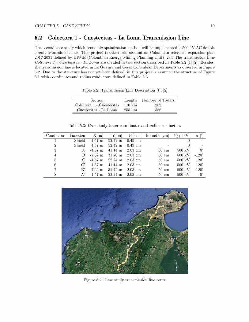
The second case study which economic optimization method will be implemented is 500 kV AC doublecircuit transmission line. This project is taken into account on Colombian reference expansion plan2017-2031 defined by UPME (Colombian Energy Mining Planning Unit) [23]. The transmission LineColectora 1 - Cuestecitas - La Loma are divided in two section described in Table 5.2 [1] [2]. Besides,the transmission line is located in La Guajira and Cesar Colombian Departments as observed in Figure5.2. Due to the structure has not yet been defined, in this project is assumed the structure of Figure5.1 with coordinates and radius conductors defined in Table 5.3.

Table 5.2: Transmission Line Description [1], [2]

Section Length Number of TowersColectora 1 - Cuestecitas 110 km 252Cuestecitas - La Loma 255 km 586

Table 5.3: Case study tower coordinates and radius conductors

Conductor Function X [m] Y [m] R [cm] Boundle [cm] VLL [kV] α [°]1 Shield -4.57 m 52.42 m 0.49 cm - 0 -2 Shield 4.57 m 52.42 m 0.49 cm - 0 -3 A -4.57 m 41.14 m 2.03 cm 50 cm 500 kV 0°4 B -7.62 m 31.70 m 2.03 cm 50 cm 500 kV -120°5 C -4.57 m 22.24 m 2.03 cm 50 cm 500 kV 120°6 C’ 4.57 m 41.14 m 2.03 cm 50 cm 500 kV 120°7 B’ 7.62 m 31.72 m 2.03 cm 50 cm 500 kV -120°8 A’ 4.57 m 22.24 m 2.03 cm 50 cm 500 kV 0°

Figure 5.2: Case study transmission line route

6.Results

6.1 Back Fashover Rate BFR

The back flashover rate BFR was calculated using each method described in this document subject to

average cloud to ground flash density η = 3.6 flasheskm2·year to EPRI transmission line and η = 6 flashes

km2·yearto Colectora 1 - Cuestecitas - La Loma, and grounding impulse resistance for all towers R = 20 Ω.Ground flash density for the Colombian transmission line is based on keraunic level map availableon [?]. Firstly, Table 6.1 presents the number of flashes that impact transmission line according toeach method. The differences between methods reside in the model that determine the number offlashes to the line based on the flashes cloud to ground, described in chapter 3. In the case of IEEEand CIGRE method, the method is the same. Likewise, the Monte Carlo method, the difference is dueto the stochastic nature of the model. In the case of the Colombian transmission line, the kerauniclevel is higher and therefore, the number of flashes that impact transmission line.

Table 6.1: Number of flashes to line

MethodFlash collection rate

EPRI transmission lineFlash Collection rate

Colectora 1 - La Loma - Cuestecitas

EPRI 72 flashes100km·year

121 flashes100km·year

IEEE 1243 95 flashes100km·year


CIGRE 95 flashes100km·year


Monte-Carlo 56 flashes100km·year


In the same way, Table 6.2 shows the probability of back flashover occurrence. The variation of resultsfor each method is due to two reasons. Calculation of insulation voltage differs for each method. EPRImethod use distance between tower height and topcrossarm. IEEE 1243 employ the distance betweentower height and phase height, and CIGRE uses phase distance. The second reason is the probabilitydistribution adopted which presents the major variation and sensitivity. For Colombian transmissionline, the probability of occurrence is lowest due to for 500 kV line structures, insulator length is bigger,hence CFO is major and less probable to generate back flashover.

Table 6.2: Probability of BFR occurrence

Method EPRI transmission line Colectora 1 - La Loma - CuestecitasEPRI 0.025 0.012

IEEE 1243 0.031 0.022CIGRE 0.015 0.010

Monte - Carlo 0.024 0.011Monte - Carlo 0.025 0.012

Finally, Table 6.3 contains the back flashover rate results in all methods. These results can be vali-dated with [18] and [22], which present a comparison between CIGRE and IEEE-flash methods. Thus,the Monte-Carlo method brings a higher back flashover rate to concentrate supplemental groundingelectrodes. Likewise, the IEEE method presents a major back flashover rate than CIGRE method

20

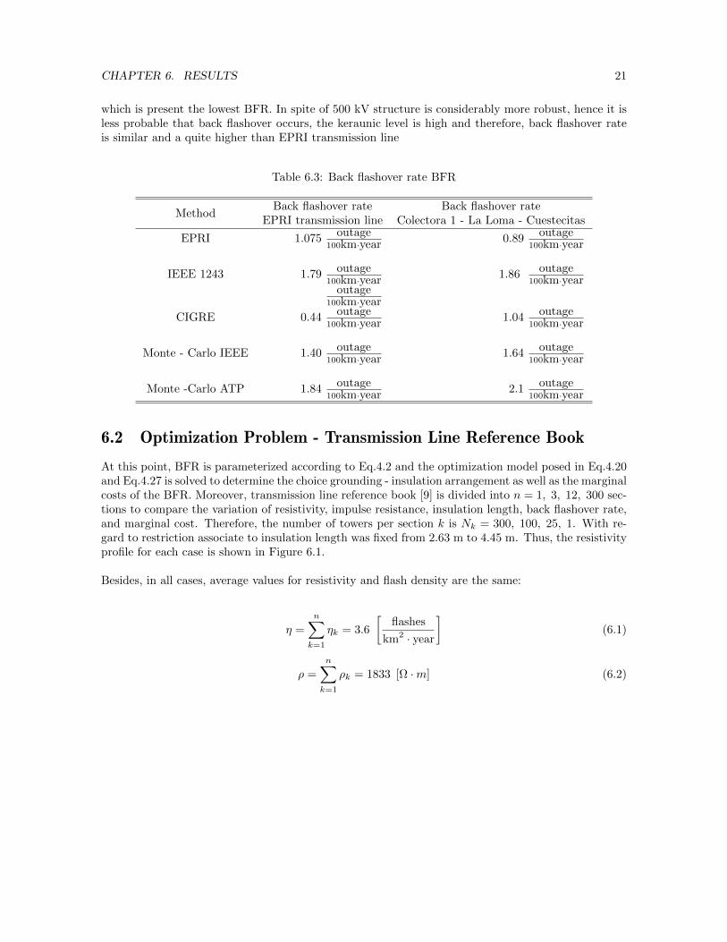
CHAPTER 6. RESULTS 21

which is present the lowest BFR. In spite of 500 kV structure is considerably more robust, hence it isless probable that back flashover occurs, the keraunic level is high and therefore, back flashover rateis similar and a quite higher than EPRI transmission line

Table 6.3: Back flashover rate BFR

MethodBack flashover rate

EPRI transmission lineBack flashover rate

Colectora 1 - La Loma - Cuestecitas

EPRI 1.075outage

100km·year0.89

outage100km·year

IEEE 1243 1.79outage

100km·year1.86

outage100km·year

outage100km·year

CIGRE 0.44outage

100km·year1.04

outage100km·year

Monte - Carlo IEEE 1.40outage

100km·year1.64

outage100km·year

Monte -Carlo ATP 1.84outage

100km·year2.1

outage100km·year

6.2 Optimization Problem - Transmission Line Reference Book

At this point, BFR is parameterized according to Eq.4.2 and the optimization model posed in Eq.4.20and Eq.4.27 is solved to determine the choice grounding - insulation arrangement as well as the marginalcosts of the BFR. Moreover, transmission line reference book [9] is divided into n = 1, 3, 12, 300 sec-tions to compare the variation of resistivity, impulse resistance, insulation length, back flashover rate,and marginal cost. Therefore, the number of towers per section k is Nk = 300, 100, 25, 1. With re-gard to restriction associate to insulation length was fixed from 2.63 m to 4.45 m. Thus, the resistivityprofile for each case is shown in Figure 6.1.

Besides, in all cases, average values for resistivity and flash density are the same:

η =

n∑k=1

ηk = 3.6

[flashes

km2 · year

](6.1)

ρ =

n∑k=1

ρk = 1833 [Ω ·m] (6.2)


0 50 100 150 200 250 300

Towers Transmission Line

500

1000

1500

2000

2500

3000

3500

4000

4500

[.m

]

k - n =1

k - n =3

k - n =12

k - n =300

Figure 6.1: Resistivity profile

Fitting factors αij of the BFR formula given in Eq. 4.2 were adjusted with m = 5 via least squares ap-proach from results obtained of multiples runs each method to compute back flashover rate with Rk andωk ranging 1 Ω to 50 Ω and 2 m to 6m. The fitting parameters to EPRI method are shown in Table 6.4.

Table 6.4: Back Flashover Parameterization Parameters αij

αij 1 2 3 4 51 2.7550 -0.0287 1.1087e-04 -1.8698e-07 1.1547e-102 0.0344 -2.2752e-05 -1.1875e-06 4.1051e-09 -3.7592e-123 0.0374 -2.9989e-04 9.6580e-07 -1.4512-09 8.4192e-134 -6.0827e-05 4.1976e-09 5.6720e-10 4.5885e-15 -1.2483e-155 -0.0287 4.5189e-08 -1.5864e-10 2.2901e-13 -1.1503e-16

Figure 6.2 shows the total cost associated to reduce back flashover rate to a prescribed value accordingto each method for 12 sections. Total cost result considers both insulation and grounding optimization.The method with the lowest cost is the CIGRE method due to presents the lowest back flashover rate,described in Table 6.3. Likewise, the IEEE method has associate the higher total cost, followed byEPRI and Monte Carlo methods.


0 0.2 0.4 0.6 0.8 1 1.2

Tk

0

3

6

9

12

15

CG

K+

CIk

[M

$]

EPRI

IEEE

Monte Carlo

CIGRE

Figure 6.2: Total cost between range from 0.1 to 1.2outage

100km·yearfor EPRI transmission line

Moreover, Figure 6.3 presents the cost of decrease back flashover rate based on each method. Thus,

for EPRI transmission line, decrease back flashover rate less than 0.4outage

100km·yeargenerate a significant

increase in marginal cost.

0 0.2 0.4 0.6 0.8 1 1.2

Tk

-140

-120

-100

-80

-60

-40

-20

0

CG

k/

Tk [M

$]

EPRI

IEEE

Monte Carlo

CIGRE

Figure 6.3: Marginal cost between range from 0.1 to 1.2outage

100km·yearfor EPRI transmission line


6.3 Optimization Problem: Colectora 1 - Cuestecitas - La Loma

To establish an adequate comparison between EPRI transmission line and Colombian case study, asection of line Colectora 1- Cuestecitas was divided into 12 sections with 21 towers per sections andspan length 436 m approximately. The optimization problem was resolved into a back flashover range

from 0.1 to 1.2outage

100km·yearfor all methods described in chapter 3. Besides, with regard to restriction

associate to insulation length was fixed from 3.42 m to 5 m. Similarly:

η =

n∑k=1

ηk = 6

[flashes

km2 · year

](6.3)

ρ =

n∑k=1

ρk = 1833 [Ω ·m] (6.4)

Therefore, Figure 6.4 shows the total cost associated to reduce back flashover to a prescribed valueaccording to each method. In this case, the total cost is thoroughly greater than EPRI transmissionline. Besides, IEEE method presets the higher total cost, followed by Monte Carlo, CIGRE and EPRImethod.

0 0.2 0.4 0.6 0.8 1 1.2

Tk

0

5

10

15

20

25

CG

K+

CIk

[M

$]

CIGRE

Monte Carlo

IEEE

EPRI

Figure 6.4: Total cost between range from 0.1 to 1.2outage

100km·yearfor colectora 1 - Cuestecitas

transmission line

Finally, Figure 6.5 shows the marginal cost of decrease back flashover rate to a prescribed value. The

limit where marginal cost increase excessively is in 0.6outage

100km·year. The above is due to the high val-

ues of the keraunic level around transmission line location. Likewise, marginal cost presents a similarbehavior for all methods, having the IEEE method the major associate incremental cost.


0 0.2 0.4 0.6 0.8 1 1.2

Tk

-18

-16

-14

-12

-10

-8

-6

-4

-2

0

CG

k/

Tk [M

$]

CIGRE

Monte Carlo

IEEE

EPRI

Figure 6.5: Marginal cost between range from 0.1 to 1.2outage

100km·yearfor Colectora 1 - Cuestecitas

transmission line


6.3.1 Limitations

It is worth to mention the limitations of the implemented method. In the first place, the insulation costmodel presents important assumptions and it is highly general and varies depending on the conditionof specific transmission line and their respective conditions. Second, due to values of resistivity profileand tower structure type are unknown, this parameter was assumed for Colectora 1 - Cuestecitas - LaLoma. Thus, for real case, it is necessary to determine the real values of each parameter aiming to getthe real total and incremental cost for the specific transmission line. Lastly, the implemented modelis suitable to design phase project, to minimize investment total cost for a prescribed back flashoverrate and the model takes importance in transmission lines with adverse terrain conditions.

6.4 Summary of results

In the Colombian Case (HVAC 500kV line) results show that CIGRE, EPRI method, IEEE Flashand Montecarlo-ATP-EMTP yield similar total and marginal cost-BFR curves. The most conser-vative result (higher costs) is the IEEE Flash method and the most optimistic one is EPRI (lowercosts). The investment cost in grounding and insulation to assure a BFR of 1 outage/100km/yearis around US$5 million (EPRI) - US$8 million (IEEE Flash). The marginal cost of a BFR of 0.2outages/100km/year is around -4, -6 million. US$/tripouts/100km/yr. This means that for highreliability standard BFR=0.2) a reduction of 0.01 outages per 100 km-yr will require an additionalinvestment of US$40000, US$60000 in mitigation measures.

When comparing both examples, it is observed that back flashover rate decreases as the voltage levelincreases. Thus, a in Colectora 1 - Cuestecitas - La Loma transmission line, BFR is less than theobserved at EPRI transmission line. This happens in spite of higher keraunic level at Colombiancase. The above is due to structures of UHV transmission line are more robust and insulator lengthincrease. Therefore, it is necessary a high lightning current considerably large to cause a back flashover,and according to probability distribution lightning current, these current values present a minimumoccurrence probability

7.ConclusionsIn this thesis, the De Oliveira/Hileman [12,15] economic optimization model was applied to determinethe total and marginal cost curves of the back flashover rate using four diffrent methods: EPRI RedBook, IEEE 1247 (Flash program), CIGRE and Montecarlo-ATP-EMTP. Two test cases were studied.

In the EPRI’s test case (HVAC 345kV line), results show that three methods (EPRI Red Book, IEEEFlash and Montecarlo-ATP-EMTP) yield very similar total and marginal cost-BFR curves. The CI-GRE method yields a more optimistic curve (lower costs) when the desired BFR is low. The investmentcost in grounding and insulation to assure a BFR of 1 outage/100km/year is around US$2.5 million.

In the Colombian Case (HVAC 500kV line) results show that CIGRE, EPRI method, IEEE Flashand Montecarlo-ATP-EMTP yield similar total and marginal cost-BFR curves. The most conser-vative result (higher costs) is the IEEE Flash method and the most optimistic one is EPRI (lowercosts). The investment cost in grounding and insulation to assure a BFR of 1 outage/100km/yearis around US$5 million (EPRI) - US$8 million (IEEE Flash). The marginal cost of a BFR of 0.2outages/100km/year is around -4, -6 million. US$/tripouts/100km/yr. This means that for highreliability standard BFR=0.2) a reduction of 0.01 outages per 100 km-yr will require an additionalinvestment of US$40000, US$60000 in mitigation measures.

When comparing both examples, it is observed that back flashover rate decreases as the voltage levelincreases. Thus, a in Colectora 1 - Cuestecitas - La Loma transmission line, BFR is less than theobserved at EPRI transmission line. This happens in spite of higher keraunic level at Colombian case.The above is due to structures of UHV transmission line are more robust and insulator length increase.Therefore, it is necessary a high lightning current considerably large to cause a back flashover, andaccording to probability distribution lightning current, these current values present a minimum occur-rence probability.

27

References[1] ANLA. Autoridad Nacional De Licencias Ambientales Auto N° 01306. page 12, 2015.

[2] ANLA. Autoridad Nacional De Licencias Ambientales Auto N° 01929. page 12, 2015.

[3] C. A. Christodoulou, L. Ekonomou, G. P. Fotis, N. Harkiolakis, and I. A. Stathopulos. Optimiza-tion of Hellenic overhead high-voltage transmission lines lightning protection. Energy, 34(4):502–509, 2009.

[4] CIGRE Working Group. Guide to procedures for estimating the lightning performance of trans-mission lines. CIGRE brochure 63, 01(October):64, 1991.

[5] S. Colectora. Proyecto UPME 06 – 2017. (01306), 2018.

[6] P. M. De Oliveira-De Jesus, D. Hernandez-Torres, and A. J. Urdaneta. Cost-Effective Opti-mization Model for Transmission Line Outage Rate Control Due to Back-Flashover Phenomena.Electric Power Components and Systems, 0(0):1–10, 2018.

[7] P. M. De Oliveira-De Jesus, D. Hernandez-Torres, and A. J. Urdaneta. Multiple-objective ap-proach for reliability improvement of electrical energy transmission systems exposed to back-flashover phenomena. Electrical Engineering, 100(4):2743–2753, 2018.

[8] L. Ekonomou, D. P. Iracleous, I. F. Gonos, and I. A. Stathopulos. An optimal design method forimproving the lightning performance of overhead high voltage transmission lines. Electric PowerSystems Research, 76(6-7):493–499, 2006.

[9] EPRI. transmission line reference book, 345kV and above. pages 545–597. 1982.

[10] F. M. Gatta, A. Geri, S. Lauria, M. MacCioni, and A. Santarpia. An ATP-EMTP Monte Carloprocedure for backflashover rate evaluation. 2012 31st International Conference on LightningProtection, ICLP 2012, (1):1–6, 2012.

[11] G. Grosser and A. Hileman. Economic Optimization of Transmission Tower Grounding andInsulation. IEEE Transactions on Power Apparatus and Systems, PAS-86(8):979–986, 2007.

[12] G. E. Grosser, A. R. Hileman, and S. Member. Economic Optimization of Transmission TowerGrounding and Insulation. (8):979–986, 1967.

[13] J. V. Hincapie. Metodologıa de optimizacion del nivel de aislamiento electrico y la resistencia depuesta a tierra en lıneas de transmision con relacion a su desempeno ante. Bdigital.Unal.Edu.Co,2017.

[14] IEEE Power Engineering Society. IEEE Std 1243-1997: IEEE Guide For Improving The lightningPerformance of Transmission Lines. 1997.

[15] P. M. D. O.-d. Jesus and S. Member. Economic Optimization of Insulation and Grounding inTransmission Systems exposed to Direct Lightning Strokes. X(X):1–10, 2017.

[16] Y. Li, Q. Yang, W. Sima, J. Li, and T. Yuan. Optimization of transmission-line route basedon lightning incidence reported by the lightning location system. IEEE Transactions on PowerDelivery, 28(3):1460–1468, 2013.

[17] MINISTERIO DE MINAS Y ENERGIA. Reglamento Tecnico De Instalaciones Electricas-Retie.page 205, 2013.

[18] C. A. Nucci. A survey on cigre and IEEE procedures for the estimation of the lightning perfor-mance of overhead transmission and distribution lines. 2010 Asia-Pacific Symposium on Electro-magnetic Compatibility, APEMC 2010, pages 1124–1133, 2010.

28

REFERENCES 29

[19] P. D. Oliveira, H. M. Khodr, J. F. Gomez, L. Ocque, A. J. Urdaneta, and S. Member. TransmissionLine Grounding System Design : An Optimization Approach. pages 1–8.

[20] S. Salman and R. Allan. Application of optimisation techniques to the design of very-high-voltagepower lines. Proceedings of the Institution of Electrical Engineers, 126(6):499, 2010.

[21] P. Sarajcev. Monte Carlo method for estimating backflashover rates on high voltage transmissionlines. Electric Power Systems Research, 119:247–257, 2015.

[22] T. Thanasaksiri. Comparison of CIGRE Method and IEEE-Flash Software for Back-flashoverRate Calculations. Procedia Computer Science, 86:445–448, 2016.

[23] Unidad de Planeacion Minero Energetica. Plan de expansion de referencia generacion -transmisionversion preliminar. Ministerio de Minas y Energıa, pages 1–343, 2017.

Documents

Presented to - Uniandes