ASSOCIATION MAPPING

Statistica: L’unica scienza che permette a esperti diversi di utilizzare informazioni uguali per trarre conclusioni diverse.

Evan Esar

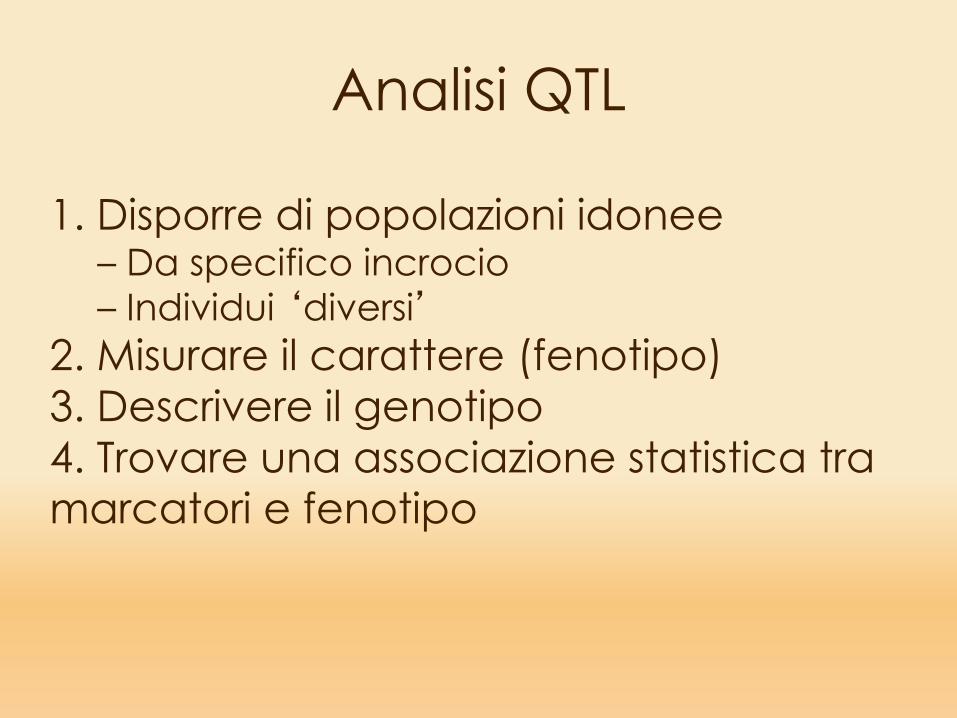
Analisi QTL

1. Disporre di popolazioni idonee– Da specifico incrocio– Individui ‘diversi’

2. Misurare il carattere (fenotipo)3. Descrivere il genotipo4. Trovare una associazione statistica tra marcatori e fenotipo

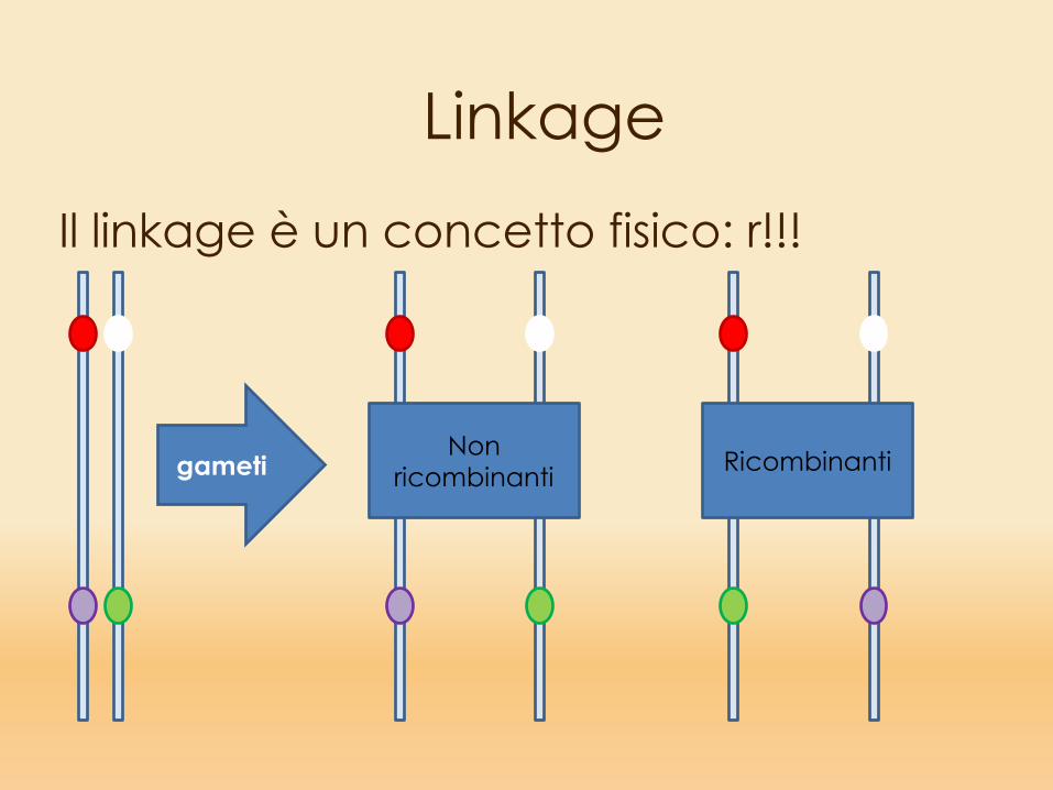
LinkageIl linkage è un concetto fisico: r!!!

gametiNon

ricombinanti Ricombinanti

Popolazioni di mappa(RILs, DH, F2…..)

1. Pochi fenotipi2. Richiedono molto tempo3. Hanno «solo» 2 alleli per locus4. «pochi» eventi possibili di ricombinazione5. Spesso basso potere di risoluzione

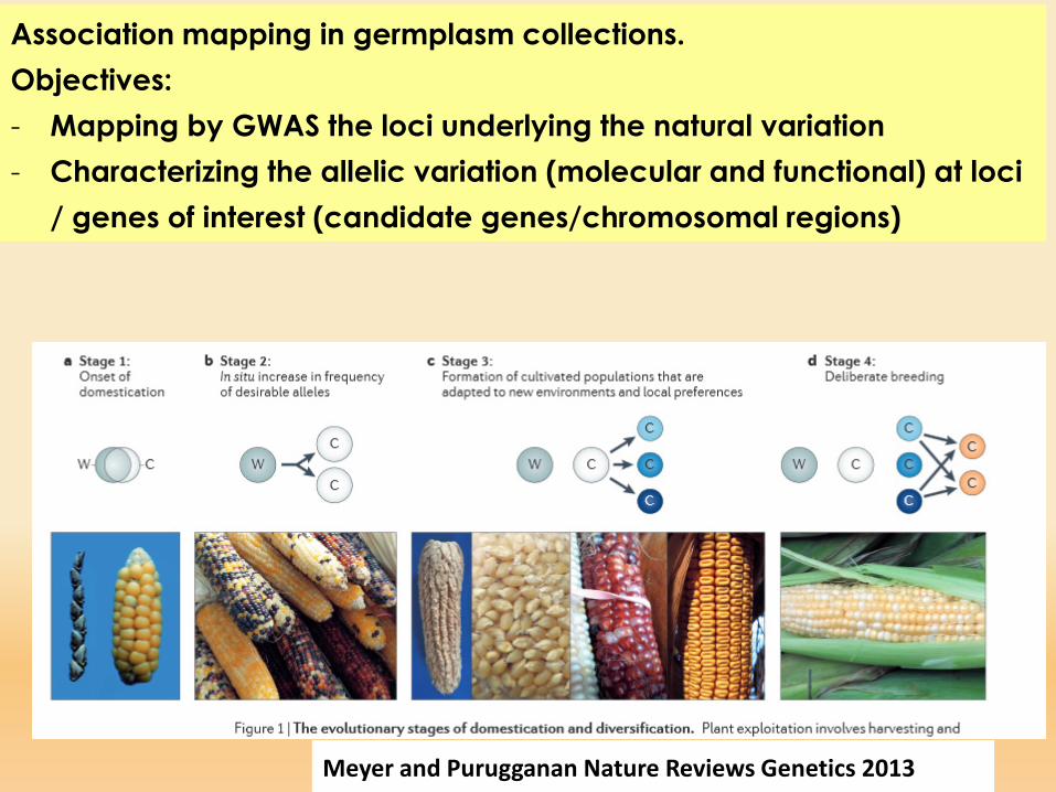
Association mapping in germplasm collections.Objectives:- Mapping by GWAS the loci underlying the natural variation- Characterizing the allelic variation (molecular and functional) at loci

/ genes of interest (candidate genes/chromosomal regions)

Meyer and Purugganan Nature Reviews Genetics 2013

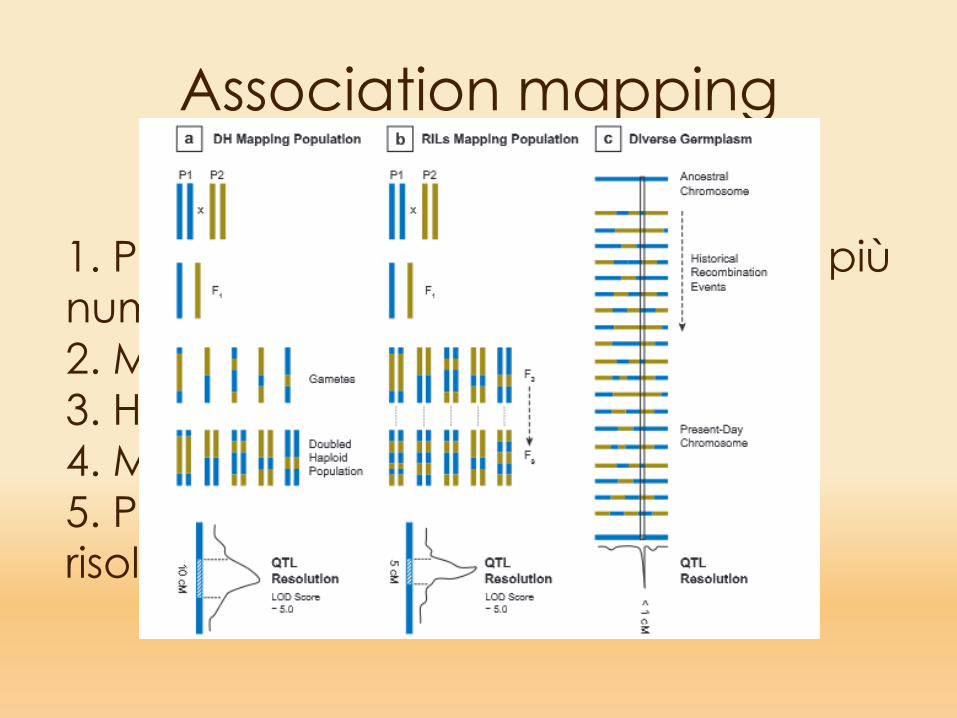
Association mapping

1. Popolazioni potenzialmente molto più numerose2. Materiale ‘già pronto’3. Hanno molti alleli per locus4. Molti eventi di ricombinazione5. Potenzialmente alto potere di risoluzione

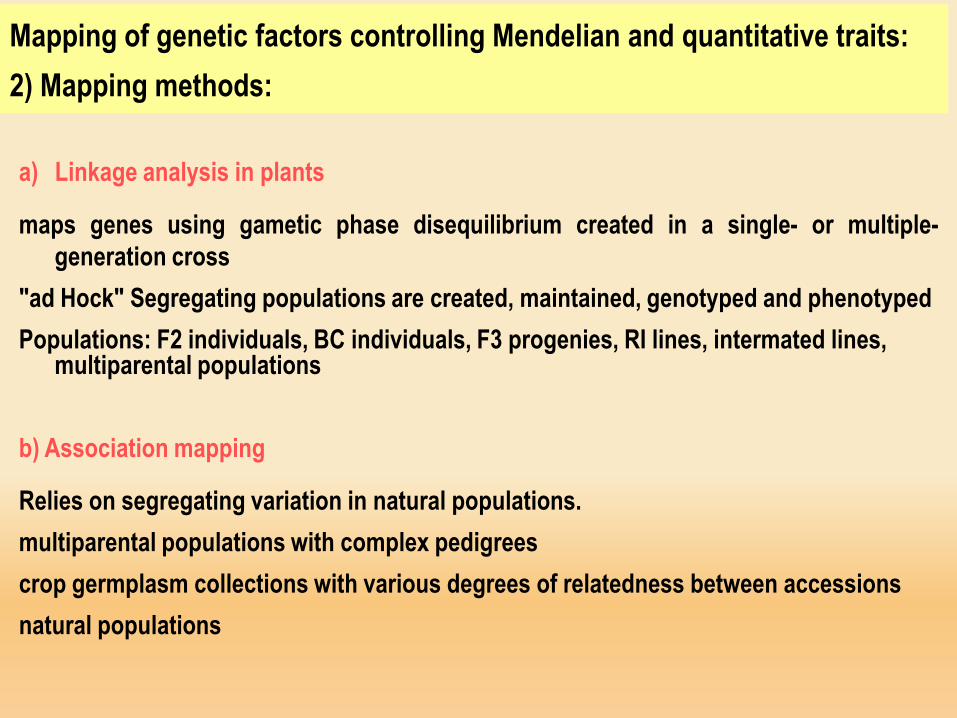
Mapping of genetic factors controlling Mendelian and quantitative traits:2) Mapping methods:

a) Linkage analysis in plants

maps genes using gametic phase disequilibrium created in a single- or multiple-generation cross

"ad Hock" Segregating populations are created, maintained, genotyped and phenotypedPopulations: F2 individuals, BC individuals, F3 progenies, RI lines, intermated lines,

multiparental populations

b) Association mapping

Relies on segregating variation in natural populations.multiparental populations with complex pedigreescrop germplasm collections with various degrees of relatedness between accessionsnatural populations

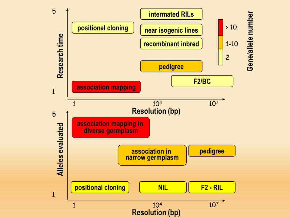
positional cloning

association mapping

pedigree

F2/BC

recombinant inbred

near isogenic lines

intermated RILs

Gene

/allel

e num

ber

2

1-10

> 10

1

5

Rese

arch

tim

e

1 104 107

Resolution (bp)association mapping in

diverse germplasm

association in narrow germplasm

pedigree

F2 - RILNILpositional cloning

1 104 107

Resolution (bp)

5

1

Allel

es ev

aluat

ed

LINKAGE DISEQUILIBRIUM

~~~

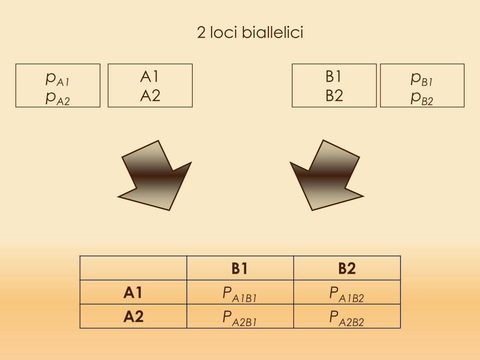
2 loci biallelici

A1A2

B1B2

pA1pA2

pB1pB2

B1 B2A1 PA1B1 PA1B2

A2 PA2B1 PA2B2

Expected frequenciesPA1B1 = pA1 pB1PA1B2 = pA1 pB2PA2B1 = pA2 pB1PA2B2 = pA2 pB2

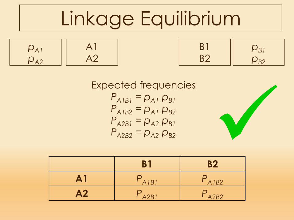
Linkage Equilibrium A1A2

B1B2

pA1pA2

pB1pB2

B1 B2A1 PA1B1 PA1B2

A2 PA2B1 PA2B2

Expected frequenciesPA1B1 = pA1 pB1PA1B2 = pA1 pB2PA2B1 = pA2 pB1PA2B2 = pA2 pB2X

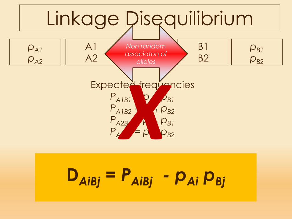
Linkage DisequilibriumA1A2

B1B2

pA1pA2

pB1pB2

Non random associaton of

alleles

B1 B2A1 PA1B1 PA1B2A2 PA2B1 PA2B2

DAiBj = PAiBj - pAi pBj

Linkage Disequilibrium

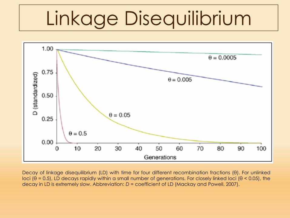
Decay of linkage disequilibrium (LD) with time for four different recombination fractions (θ). For unlinkedloci (θ = 0.5), LD decays rapidly within a small number of generations. For closely linked loci (θ < 0.05), thedecay in LD is extremely slow. Abbreviation: D = coefficient of LD (Mackay and Powell, 2007).

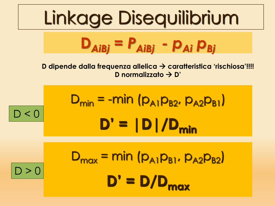
Linkage DisequilibriumDAiBj = PAiBj - pAi pBj

Dmin = -min (pA1pB2, pA2pB1)

D’ = |D|/DminD < 0

Dmax = min (pA1pB1, pA2pB2)

D’ = D/DmaxD > 0

D dipende dalla frequenza allelica caratteristica ‘rischiosa’!!!!D normalizzato D’

Linkage Disequilibrium

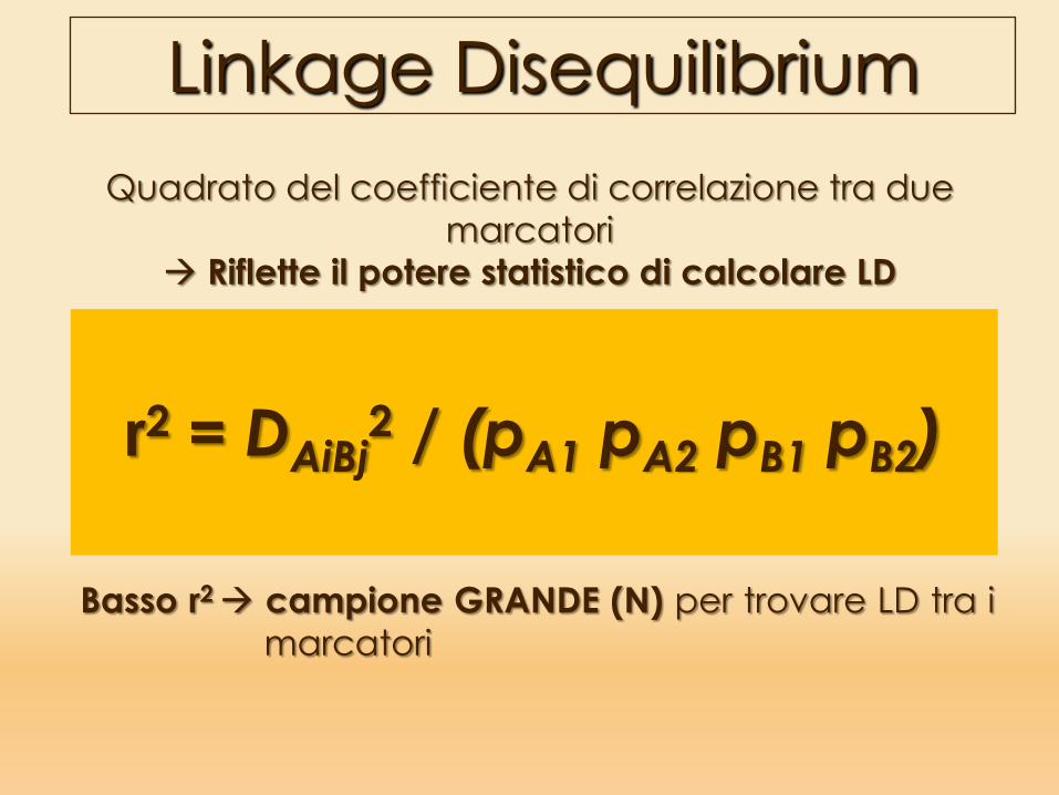
r2 = DAiBj2 / (pA1 pA2 pB1 pB2)

Quadrato del coefficiente di correlazione tra due marcatori

Riflette il potere statistico di calcolare LD

Basso r2 campione GRANDE (N) per trovare LD tra imarcatori

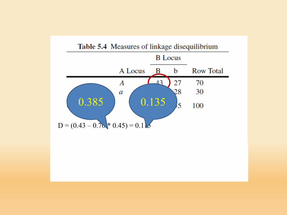
D = (0.43 – 0.70 * 0.45) = 0.115Dmax = min (0.70 * 0.55, 0.30 * 0.45) = 0.135D’ = 0.115 / 0.135 = 0.8581r2 = (0.115)2 / 0.70 * 0.30 * 0.55 * 0.45 = 0.2545

0.385 0.135

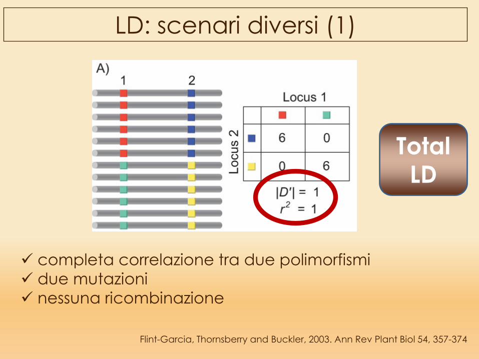
Flint-Garcia, Thornsberry and Buckler, 2003. Ann Rev Plant Biol 54, 357-374

LD: scenari diversi (1)

completa correlazione tra due polimorfismi due mutazioni nessuna ricombinazione

Total LD

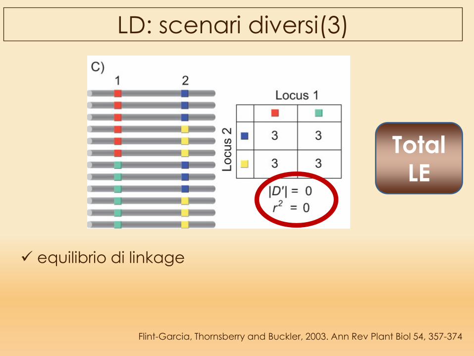
Flint-Garcia, Thornsberry and Buckler, 2003. Ann Rev Plant Biol 54, 357-374

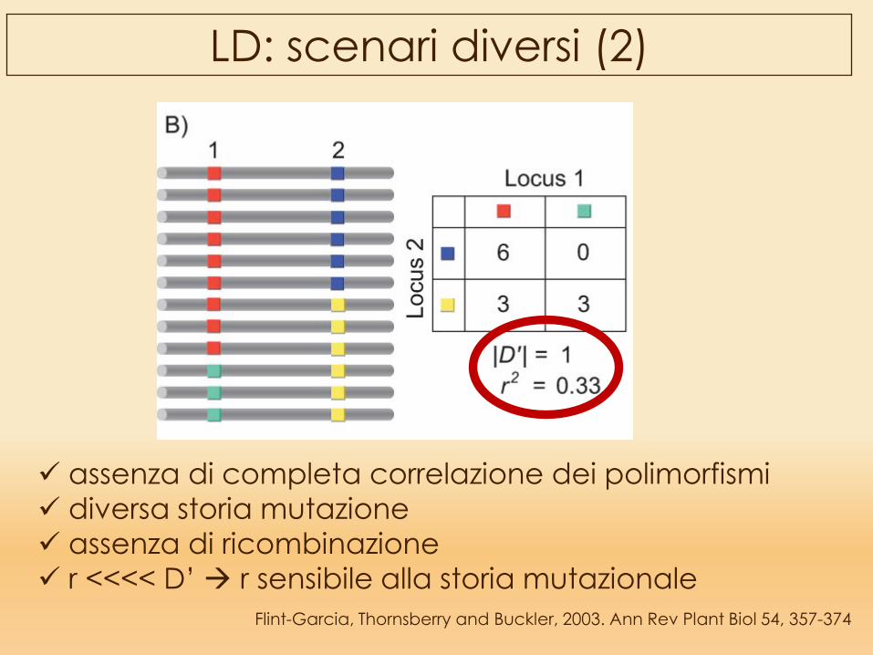
LD: scenari diversi (2)

assenza di completa correlazione dei polimorfismi diversa storia mutazione assenza di ricombinazione r <<<< D’ r sensibile alla storia mutazionale

Flint-Garcia, Thornsberry and Buckler, 2003. Ann Rev Plant Biol 54, 357-374

LD: scenari diversi(3)

equilibrio di linkage

Total LE

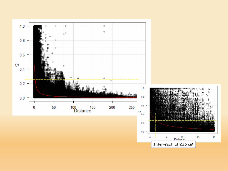
Inter-sect at 2.16 cM

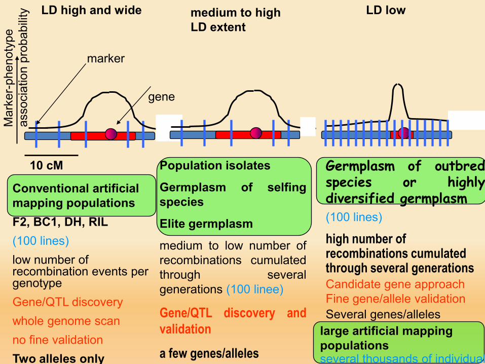
LD high and wide

Conventional artificial mapping populationsF2, BC1, DH, RIL(100 lines)low number of recombination events per genotypeGene/QTL discovery whole genome scanno fine validationTwo alleles only

large artificial mapping populationsseveral thousands of individual

gene

Population isolates

Germplasm of selfingspecies

Elite germplasm

medium to low number ofrecombinations cumulatedthrough severalgenerations (100 linee)

Gene/QTL discovery andvalidation

a few genes/alleles

LD lowmedium to high LD extent

10 cM

marker

Mar

ker-p

heno

type

as

soci

atio

n pr

obab

ility

Germplasm of outbredspecies or highlydiversified germplasm(100 lines)

high number of recombinations cumulated through several generationsCandidate gene approachFine gene/allele validationSeveral genes/alleles

Species Mating system, germplasm and LD range (average distance where r2 = 0.10)Human Outcrossing- Nigerian: 5 kb- European: 80 kbCattle Outcrossing: 10 cMDrosophila Outcrossing: <1 kbMaize Outcrossing- Diverse maize: 1 kb or less- Diverse inbred lines: 1.5 kb- Elite (cultivated) lines: > 100 kbArabidopsis Selfing: 250 kbSugarcane Outcrossing/vegetative: 10 cM propagation

Wheat and Barley selfing- Diverse barley: less than 1 cM - Elite (cultivated) germplasm up to 1-20 cM up to 60 cM

Haplotype blocks: extensive regions showing no recombinations and inherited from a know "foundation genotype"

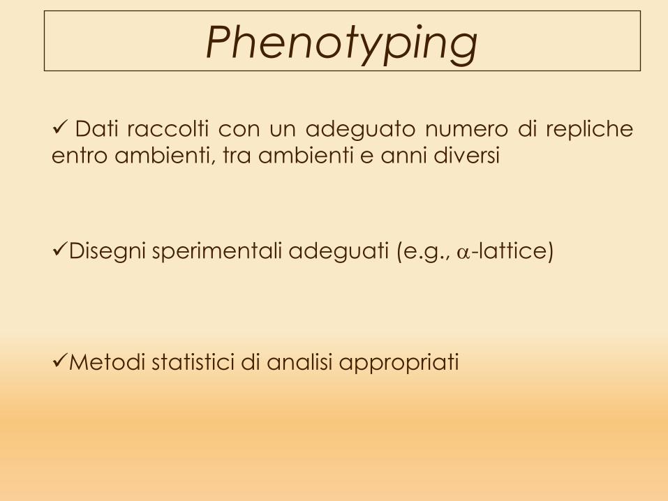
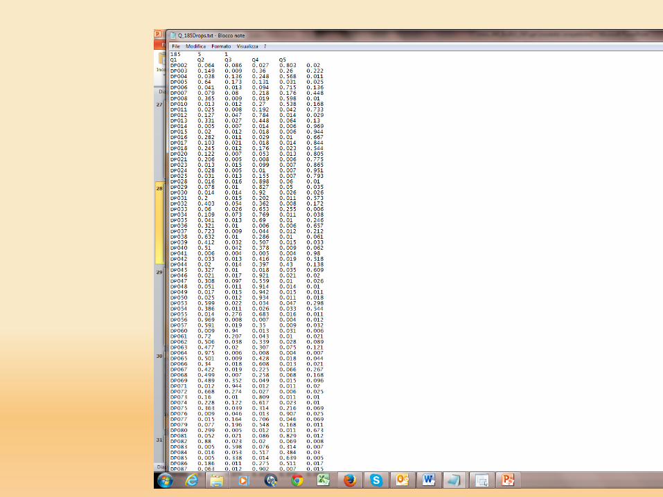
Phenotyping

Dati raccolti con un adeguato numero di replicheentro ambienti, tra ambienti e anni diversi

Disegni sperimentali adeguati (e.g., α-lattice)

Metodi statistici di analisi appropriati

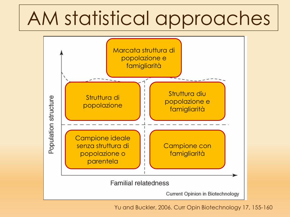
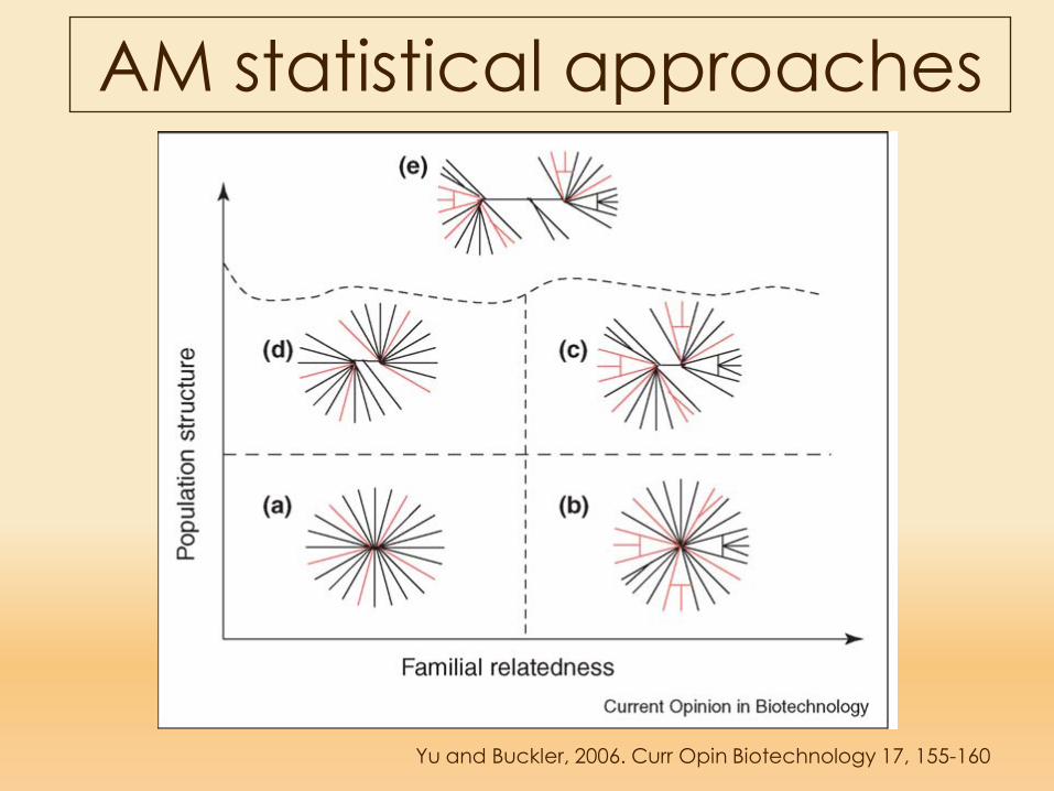
AM statistical approaches

Yu and Buckler, 2006. Curr Opin Biotechnology 17, 155-160

Campione ideale senza struttura di popolazione o

parentela

Campione con famigliarità

Struttura di popolazione

Marcata struttura di popolazione e

famigliarità

Struttura diu popolazione e

famigliarità

AM statistical approaches

Yu and Buckler, 2006. Curr Opin Biotechnology 17, 155-160

When population subdivision is present, it ispossible to find statistical associations between a disease phenotype and arbitrary markers that have no physical linkage to causative loci

Such associations occur because population subdivision (or any other form of nonrandom mating) permits marker-allele frequencies to vary among segments of the population, as the result of genetic drift or founder effects (Slatkin 1991).

Pop structure causes: - natural selection (e.g. main adaptation traits: vernalization and photoperiod sensitivity)- breeder's selection (based on ideotypes, particularly in inbred crops, founders are successfull cultivars)

Linkage disequilibrium and population structure

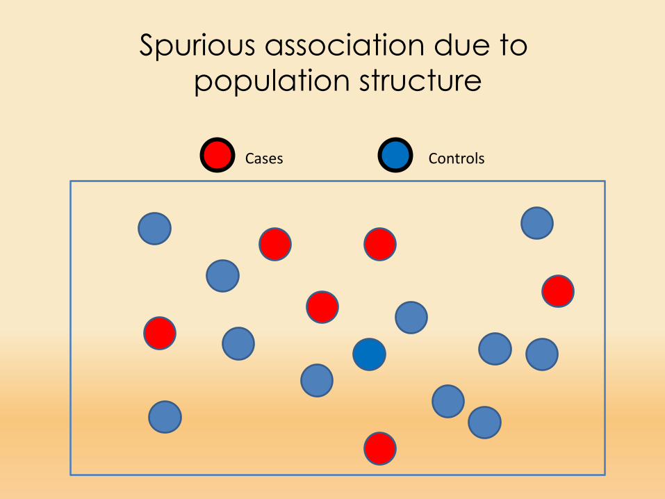
Cases Controls

Spurious association due to population structure

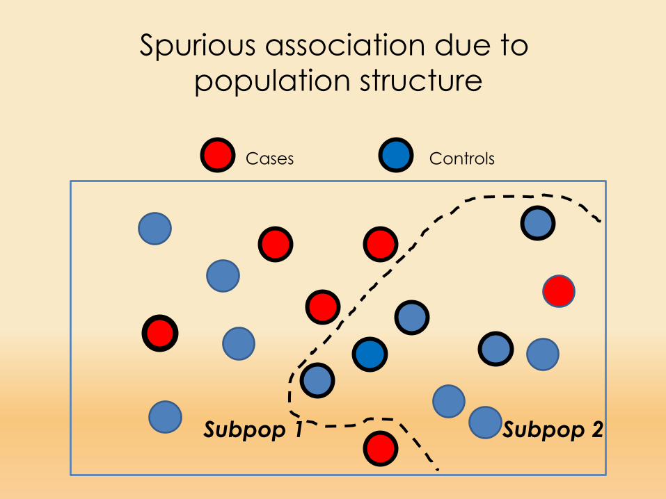
Cases Controls

Subpop 1 Subpop 2

Spurious association due to population structure

Chr. xx

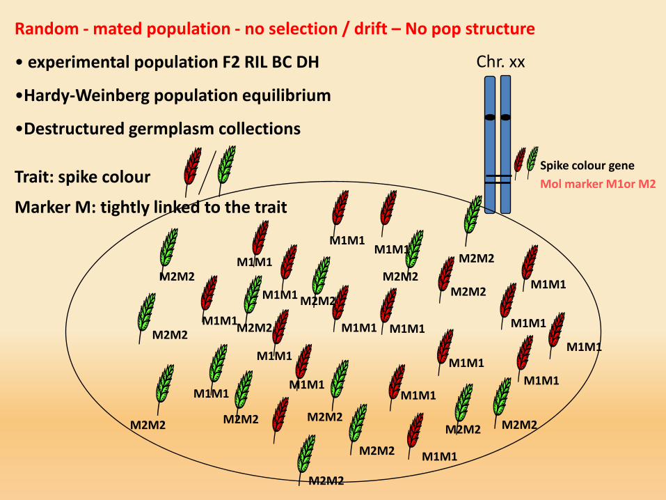
Random - mated population - no selection / drift – No pop structure

• experimental population F2 RIL BC DH

•Hardy-Weinberg population equilibrium

•Destructured germplasm collections

Mol marker M1or M2

M1M1

M2M2

M2M2

M2M2

M2M2M2M2M2M2

M1M1

M1M1M1M1

M1M1

M2M2 M1M1

M1M1

M1M1

M1M1

M1M1

M1M1M1M1

M1M1

M1M1

M1M1

M1M1

M1M1

M2M2

M2M2

M2M2

M2M2

M2M2M2M2

M2M2

Trait: spike colour

Marker M: tightly linked to the trait

Spike colour gene

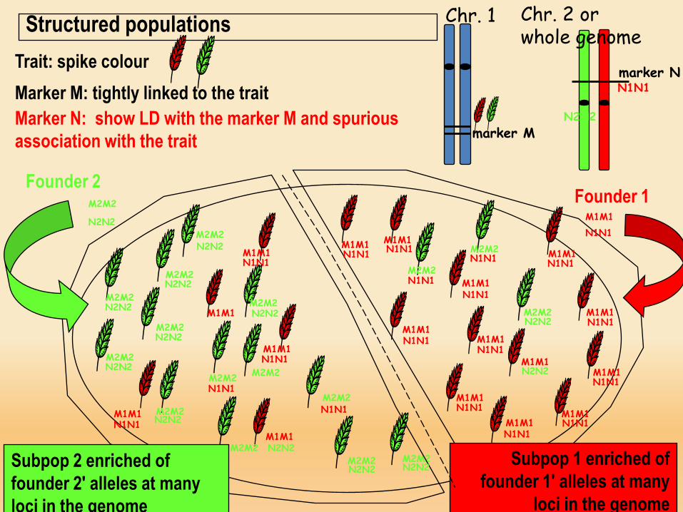
Chr. 1Structured populations

marker M

M2M2M2M2

M2M2

M2M2

M2M2

M2M2

M1M1

M1M1

M1M1

M1M1

M1M1

M1M1M1M1

M1M1

M1M1

M1M1

M1M1

M1M1

M1M1

M1M1

M1M1

M2M2

M2M2

M2M2

M2M2

M2M2

M2M2

M2M2

M1M1

M1M1M2M2

M2M2

Founder 2

marker N

Founder 1

M2M2

N2N2

N1N1

N1N1

N1N1

N1N1

N1N1

N1N1

N1N1N1N1

N2N2

N2N2

N1N1

N1N1

N1N1 N1N1

N1N1

N1N1

N2N2

N2N2

N2N2

N2N2

N2N2

N2N2

N2N2

N1N1

N2N2

N2N2

N2N2

N2N2

N1N1

N1N1N1N1

M2M2M1M1

Subpop 2 enriched of founder 2' alleles at many loci in the genome

Subpop 1 enriched of founder 1' alleles at many

loci in the genome

Trait: spike colourMarker M: tightly linked to the traitMarker N: show LD with the marker M and spurious association with the trait

N1N1

N1N1

Chr. 2 or whole genome

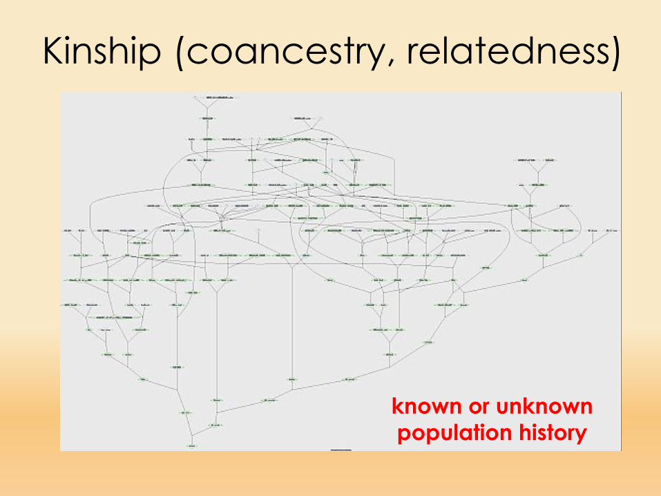
known or unknown population history

Kinship (coancestry, relatedness)

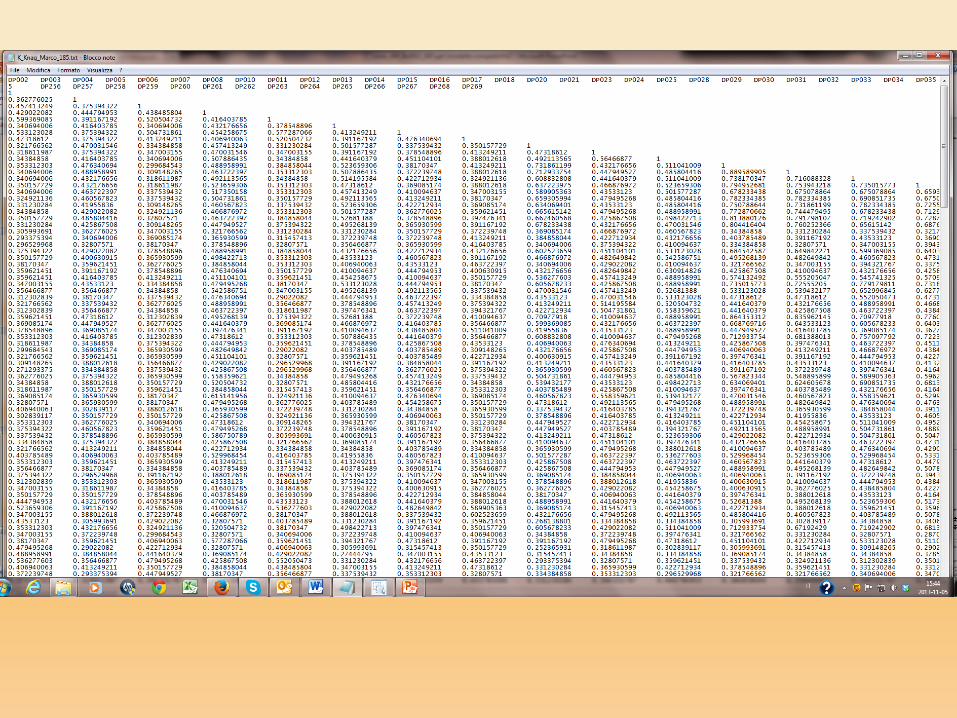
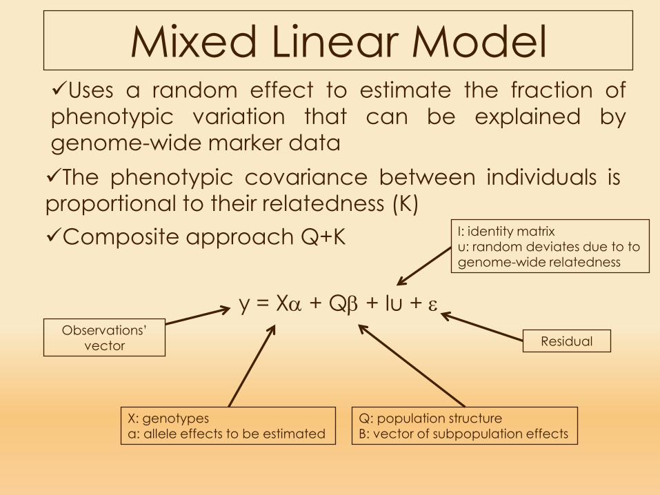
Mixed Linear Model

The phenotypic covariance between individuals isproportional to their relatedness (K)Composite approach Q+K

y = Xα + Qβ + Iu + εObservations’

vector

X: genotypesa: allele effects to be estimated

Q: population structureB: vector of subpopulation effects

Residual

I: identity matrixu: random deviates due to to genome-wide relatedness

Uses a random effect to estimate the fraction ofphenotypic variation that can be explained bygenome-wide marker data

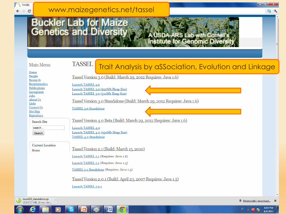
www.maizegenetics.net/tassel

Trait Analysis by aSSociation, Evolution and Linkage