Presentation-Boom and Bust in Oil Prices

8/3/2019 Presentation-Boom and Bust in Oil Prices

http://slidepdf.com/reader/full/presentation-boom-and-bust-in-oil-prices 1/25

Introduction Investor Flows and Speculation New Evidence on Investor Flows and Oil Prices References

Investor Flows and the2008 Boom/Bust in Oil Prices

Kenneth J. Singleton

Graduate School of BusinessStanford University

August, 2011




Investor Flows, Speculation, and Oil Prices

The role of speculation (broadly construed) in the dramaticrise and subsequent sharp decline in oil prices during 2008?

Many attribute these swings to changes in fundamentals of supply and demand, within representative agent models.

At the same time there is mounting evidence of the“financialization” of commodity markets.

Objective: investigate the impact of investor flows andfinancial market conditions on crude-oil futures prices.




Heterogeneity and Investor Flows

The prototypical dynamic models referenced in discussions of the oil boom (e.g., Hamilton (2009), Pirrong (2009)) haverepresentative agent-types (producer, storage operator,commercial consumer, etc.).

Moreover, they do not allow for learning under imperfectinformation, heterogeneity of beliefs, and capital market andagency-related frictions that limit arbitrage activity.

As such, they abstract entirely from the consequent rationalmotives for many categories of market participants tospeculate in commodity markets based on their individualcircumstances and views about fundamental economic factors.




Inferred Commodity Index Long Positions (Dash →)Against NYMEX WTI Futures (Solid ← )

250,000

350,000

450,000

550,000

650,000

750,000

850,000

$0.00

$25.00

$50.00

$75.00

$100.00

$125.00

$150.00

3 - J a n - 0 7

3 - M a r - 0 7

3 - M a y - 0 7

3 - J u l - 0 7

3 - S e p - 0 7

3 - N o v - 0 7

3 - J a n - 0 8

3 - M a r - 0 8

3 - M a y - 0 8

3 - J u l - 0 8

3 - S e p - 0 8

3 - N o v - 0 8

3 - J a n - 0 9

3 - M a r - 0 9

3 - M a y - 0 9

3 - J u l - 0 9

3 - S e p - 0 9

3 - N o v - 0 9

3 - J a n - 1 0

C o n t r a c t s o f 1 0 0 0 ' s o

f B a r r e l s

W T I P r i c e P e r B a r r e l




Financialization of Commodities: What Do We Know?

Tang and Xiong (2011) show that, after 2004, agriculturalcommodities that are part of the GSCI and DJ-AIG indicesbecame much more responsive to shocks to a world equityindex, changes in the U.S. dollar exchange rate, and oil prices.

Using proprietary data from the CFTC, Buyuksahin and Robe(2011) link increased high-frequency correlations among equityand commodity returns to trading patterns of hedge funds.

Less formally, Masters (2009) attributes price movements to

flows into crude oil positions by index investors.

Mou (2010) documents substantial impacts on prices of the“roll strategies” employed by index funds– index investorsbear large implicit transactions costs.

S O




Speculation and Booms/Busts in Commodity Prices

Absent arbitrage opportunities and near stock-out conditions

in a commodity market:

S t = E Qt

e−

T t(rs−Cs) dsS T

,

S t denotes the price of crude oil S t,Ct denotes the convenience yield net of storage costs,E Qt denotes the expectation of market participants under the

risk-neutral pricing distribution.

An implication of S t drifting at the rate (rt − Ct)S t dt.

Additionally, the futures price for delivery of a commodity atdate T > t is related to S T according to

F T

t= E

Q

t[S

T ] .

I d i I Fl d S l i N E id I Fl d Oil P i R f




The Futures-Spot Basis

Rearranging these expressions gives

F T t

S t=

1 −CovQt

e T

tCs ds, e−

T

trs ds ST

St

BT

t E Qt

e T

tCs ds

−

1

BT t

×CovQt

e−

T

trs ds,

S T

S t

,

where BT t denotes the price of a zero coupon bond.

If the covariance terms are negligible, then (approximately)

F T t − S t

S t ≈ yT

t (T − t)− ln E Q

t

e

T

t

Cs ds,

where yT t is the continuously compounded yield on a zero of maturity (T − t) periods.

I t d ti I t Fl d S l ti N E id I t Fl d Oil P i R f




Representative Risk-Neutral Market Participants?

Most of the extant model-based interpretations of the oil price

boom focus on:representative risk-neutral producers and refiners, and

they arrive at similar expressions, but with

the expectation E Qt replaced by E Pt , the expectation of market

participants under the historical distribution.





Representative Risk-Neutral Market Participants?

Most of the extant model-based interpretations of the oil price

boom focus on:representative risk-neutral producers and refiners, and

they arrive at similar expressions, but with

the expectation E Qt replaced by E Pt , the expectation of market

participants under the historical distribution.

If refiners and investors are heterogeneous and:

risk averse or

they face capital constraints that lead them to behaveeffectively as if they are risk averse, and

different classes of investors hold different views about futureoil-market fundamentals,

then risk-premiums and forecast errors will impact futures

and, thereby, spot prices.





Accommodating Risk Premiums andInformational Heterogeneity

Market risk premium: RP T t ≡

E Qt [S T ]−E Pt [S T ]

, T > t.

For a short time interval [t, τ ] over which r and C areapproximately constant:

E Pt [S τ ]− S t

S t− yτ t (τ − t) ≈ Ct (τ − t)−RP τ t .

Thus, expected excess returns in the spot commodity market

depend on both convenience yields and risk premiums.

The same will in general be true of expected excess returns inthe futures market, the percentage changes in the price of afuture contract, adjusted for roll dates.





Heterogeniety Version I:Wealth-Weighted Futures Prices

Suppose market participants hold different beliefs and havedifferent purchasing powers.

By analogy to Xiong and Yan (2010), if log S t is an affinefunction of risk factors X t that follow an affine process, then

we expect futures prices to take a form similar to

F T t =

i

ωiea(T −t)+bX(T −t)Xt+bθ(T −t)θi ,

ωi is the wealth allocation of investor i,θi summarizes investor i’s beliefs about the state of theeconomy X t.

As beliefs and wealths change, so will the futures prices.





Heterogeneity Version II:Forecasting the Forecasts of Others

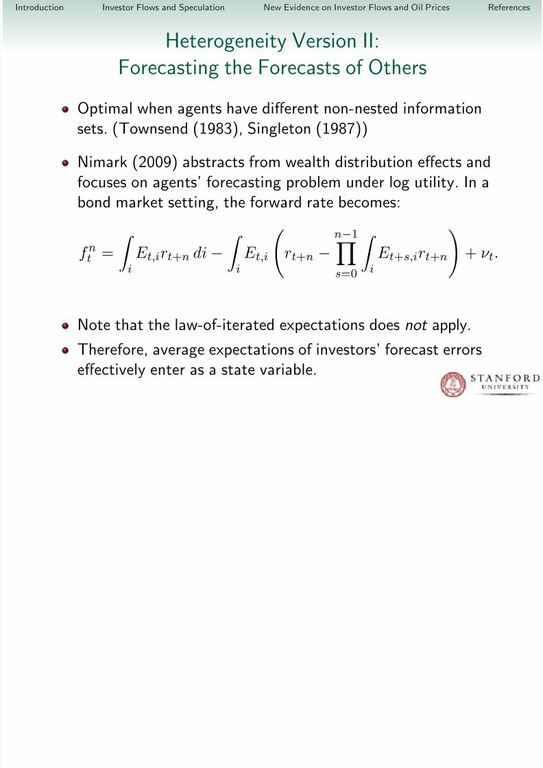
Optimal when agents have different non-nested informationsets. (Townsend (1983), Singleton (1987))

Nimark (2009) abstracts from wealth distribution effects andfocuses on agents’ forecasting problem under log utility. In abond market setting, the forward rate becomes:

f nt =

i

E t,irt+n di −

i

E t,i

rt+n −

n−1

s=0 i

E t+s,irt+n

+ ν t.

Note that the law-of-iterated expectations does not apply.

Therefore, average expectations of investors’ forecast errorseffectively enter as a state variable.




p

Implications for Commodity Pricing

Surely participants in oil market held different views abouteconomic growth, global demand and supply of oil, inventorypositions domestically and in emerging economies, etc.

Consequently, averaging across investors will typically give i

E iPt [S τ ]− S t

S t− yτ t (T − t) ≈ C̃t (T − t)− R̃P

τ

t + E τ t ,

where i indexes investors and E τ t captures the effects of

forecast errors and/or limits to arbitrage.

Expect projections of realized “excess returns” to potentiallycapture aspects of all of these ingredients?




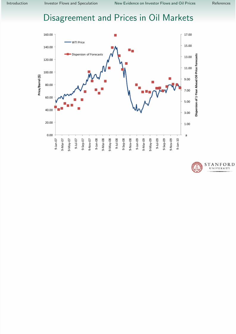
Disagreement and Prices in Oil Markets

5.00

7.00

9.00

11.00

13.00

15.00

17.00

60.00

80.00

100.00

120.00

140.00

160.00

n o f 1

‐ Y e a r A h e

a d O i l ‐ P r i c e F o r e c a s t s

P r i c e / B a r

r e l ( $ )

WTI Price

Dispersion of Forecasts

‐1.00

1.00

3.00

5.00

7.00

9.00

11.00

13.00

15.00

17.00

0.00

20.00

40.00

60.00

80.00

100.00

120.00

140.00

160.00

9 ‐

J a n ‐

0 7

9 ‐

M a r ‐ 0 7

9 ‐

M a y ‐

0 7

9 ‐

J u l ‐ 0 7

9 ‐

S e p ‐

0 7

9 ‐

N o v ‐

0 7

9 ‐

J a n ‐

0 8

9 ‐

M a r ‐ 0 8

9 ‐

M a y ‐

0 8

9 ‐

J u l ‐ 0 8

9 ‐

S e p ‐

0 8

9 ‐

N o v ‐

0 8

9 ‐

J a n ‐

0 9

9 ‐

M a r ‐ 0 9

9 ‐

M a y ‐

0 9

9 ‐

J u l ‐ 0 9

9 ‐

S e p ‐

0 9

9 ‐

N o v ‐

0 9

9 ‐

J a n ‐

1 0

D i s p e r s i o n o f 1

‐ Y e a r A h e

a d O i l ‐ P r i c e F o r e c a s t s

P r i c e / B a r

r e l ( $ )

WTI Price

Dispersion of Forecasts

a




Relative Disagreement about Oil Prices andGlobal (G7 + BRIC) GDP Growth

5

10

15

20

25

30

35

40

45

O i l S t d / G D P S t d

0

5

10

15

20

25

30

35

40

45

F e b r u a r y

‐ 0 7

A p r i l ‐ 0 7

J u n e

‐ 0 7

A u g u s t

‐ 0 7

O c t o b e r

‐ 0 7

D e c e m b e r

‐ 0 7

F e b r u a r y

‐ 0 8

A p r i l ‐ 0 8

J u n e

‐ 0 8

A u g u s t

‐ 0 8

O c t o b e r

‐ 0 8

D e c e m b e r

‐ 0 8

F e b r u a r y

‐ 0 9

A p r i l ‐ 0 9

J u n e

‐ 0 9

A u g u s t

‐ 0 9

O c t o b e r

‐ 0 9

D e c e m b e r

‐ 0 9

F e b r u a r y

‐ 1 0

O i l S t d / G D P S t d




New Evidence on Investor Flows and Oil Prices

RSPn and REMn: the n-week returns on the S&P500 andthe MSCI Emerging Asia indices, respectively.

IIP13: the thirteen-week change in the imputed positions of index investors in millions, computed using the samealgorithm as in Masters (2009).

MMSPD13: the thirteen-week change in managed-moneyspread positions in millions, as constructed by the CFTC.




More Conditioning Variables

REPOn: the n-week change in overnight repo positions onTreasury bonds by primary dealers.

OI13: the thirteen-week change in aggregate open interest.

AVBASn: the n-week change in basis averaged across thematurities {1, 3, 6, 9, 12, 15, 18, 21, 24} months.

The basis is a proxy for convenience yield– more later.




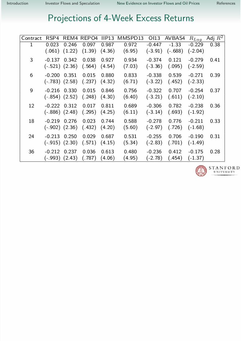
Linear Projections

ERmM t+n(n) = µnm + ΠnmX t + ΨnmERmM t(n) + εm,t+n(n),

ERmM t(n): realized excess return for an n-week investmenthorizon on a futures position that expires in m months.

X t is the set of predictor variables.

Weekly data over the sample period September 12, 2006through January 12, 2010.

Robust standard errors allowing for heteroskedasticity andserial correlation.




Projections of 1-Week Excess Returns

Contract RSP1 REM1 REPO1 IIP13 MMSPD13 OI13 AVBAS1 RLag Adj R2

1 0.332 -0.342 -0.201 0.272 0.357 -0.103 -4.165 -0.219 0.27(1.44) (-2.44) (-2.89) (3.51) (4.36) (-2.17) (-6.26) (-2.05)

3 0.361 -0.242 -0.170 0.218 0.284 -0.082 -3.661 -0.152 0.27(1.99) (-2.02) (-2.76) (3.71) (4.43) (-1.87) (-6.48) (-2.10)

6 0.391 -0.261 -0.150 0.197 0.245 -0.072 -3.022 -0.105 0.25(2.35) (-2.27) (-2.64) (3.49) (4.14) (-1.74) (-5.59) (-1.62)

9 0.424 -0.275 -0.142 0.187 0.222 -0.067 -2.551 -0.090 0.24(2.67) (-2.46) (-2.58) (3.45) (3.95) (-1.73) (-4.72) (-1.40)

12 0.437 -0.283 -0.133 0.179 0.202 -0.064 -2.141 -0.075 0.22(2.84) (-2.60) (-2.49) (3.42) (3.83) (-1.73) (-3.97) (-1.14)

18 0.430 -0.286 -0.119 0.166 0.174 -0.058 -1.657 -0.054 0.20

(2.99) (-2.79) (-2.35) (3.42) (3.61) (-1.72) (-3.13) (-0.75)24 0.412 -0.287 -0.107 0.157 0.159 -0.053 -1.329 -0.046 0.18

(2.98) (-2.87) (-2.21) (3.46) (3.40) (-1.67) (-2.60) (-0.59)

36 0.378 -0.294 -0.093 0.145 0.144 -0.048 -0.981 -0.033 0.16(2.85) (-2.99) (-2.05) (3.52) (3.02) (-1.60) (-2.10) (-0.40)




Projections of 4-Week Excess Returns

Contract RSP4 REM4 REPO4 IIP13 MMSPD13 OI13 AVBAS4 RLag Adj R2

1 0.023 0.246 0.097 0.987 0.972 -0.447 -1.33 -0.229 0.38(.061) (1.22) (1.39) (4.36) (6.95) (-3.91) (-.688) (-2.04)

3 -0.137 0.342 0.038 0.927 0.934 -0.374 0.121 -0.279 0.41(-.521) (2.36) (.564) (4.54) (7.03) (-3.36) (.095) (-2.59)

6 -0.200 0.351 0.015 0.880 0.833 -0.338 0.539 -0.271 0.39(-.783) (2.58) (.237) (4.32) (6.71) (-3.22) (.452) (-2.33)

9 -0.216 0.330 0.015 0.846 0.756 -0.322 0.707 -0.254 0.37(-.854) (2.52) (.248) (4.30) (6.40) (-3.21) (.611) (-2.10)

12 -0.222 0.312 0.017 0.811 0.689 -0.306 0.782 -0.238 0.36(-.886) (2.48) (.295) (4.25) (6.11) (-3.14) (.693) (-1.92)

18 -0.219 0.276 0.023 0.744 0.588 -0.278 0.776 -0.211 0.33

(-.902) (2.36) (.432) (4.20) (5.60) (-2.97) (.726) (-1.68)24 -0.213 0.250 0.029 0.687 0.531 -0.255 0.706 -0.190 0.31

(-.915) (2.30) (.571) (4.15) (5.34) (-2.83) (.701) (-1.49)

36 -0.212 0.237 0.036 0.613 0.480 -0.236 0.412 -0.175 0.28(-.993) (2.43) (.787) (4.06) (4.95) (-2.78) (.454) (-1.37)




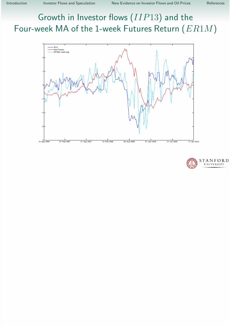
Growth in Investor flows (IIP 13) and theFour-week MA of the 1-week Futures Return (ER1M )

12−Sep−2006 27−Feb−2007 21−Aug−2007 12−Feb−2008 05−Aug−2008 27−Jan−2009 21−Jul−2009 12−Jan−2010−4

−3

−2

−1

0

1

2

3

IIP13

Near Futures

ER1M(4−week avg)




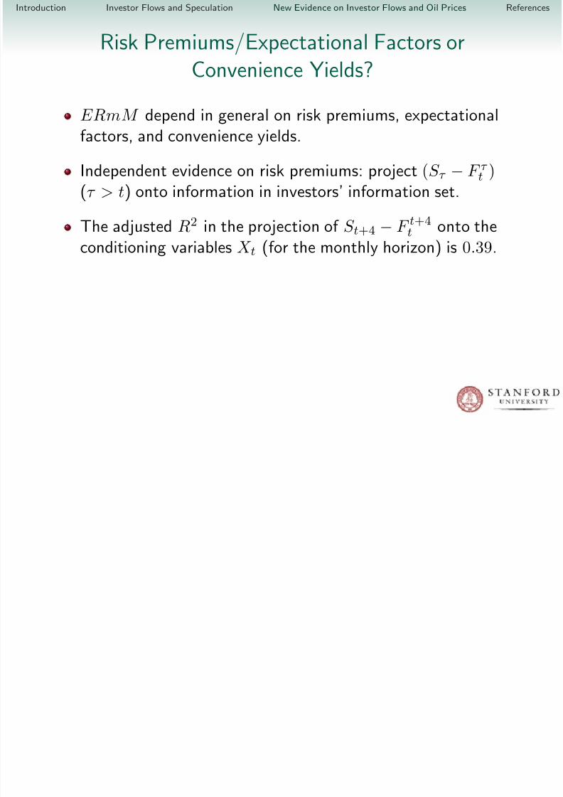
Risk Premiums/Expectational Factors orConvenience Yields?

ERmM depend in general on risk premiums, expectationalfactors, and convenience yields.

Independent evidence on risk premiums: project (S τ − F τ t )(τ > t) onto information in investors’ information set.

The adjusted R2 in the projection of S t+4 − F t+4t onto theconditioning variables X t (for the monthly horizon) is 0.39.




Risk Premiums/Expectational Factors orConvenience Yields?

ERmM depend in general on risk premiums, expectationalfactors, and convenience yields.

Independent evidence on risk premiums: project (S τ − F τ t )(τ > t) onto information in investors’ information set.

The adjusted R2 in the projection of S t+4 − F t+4t onto theconditioning variables X t (for the monthly horizon) is 0.39.

Only IIP 13 and M M S P D13 enter with statistically

significant coefficients ⇒ impacting commodity prices throughrisk premiums or speculative expectational terms?

Emerging market equity returns and open interest shaped thefutures curve, but not so much spot market risk premiums.


B k hi B d M R b 2011 “D “P Oil” M ?



Buyuksahin, B., and M. Robe, 2011, “Does “Paper Oil” Matter?Energy Markets’ Financialization and Equity-CommodityCo-Movements,” working paper, International Energy Agency.

Hamilton, J., 2009, “Causes and Consequences of the Oil Shock of 2007-08,” Brookings Papers on Economic Activity .

Masters, M., 2009, “Testimony Before the Commodity FuturesTrading Commission,” working paper, Commodity FuturesTrading Commission.

Mou, Y., 2010, “Limits to Arbitrage and Commodity IndexInvestments: Front-Running the Goldman Roll,” working paper,Columbia Business School.

Nimark, K., 2009, “Speculative Dynamics in the Term Structure of Interest rates,” working paper, Universitat Pompeu Fabra.

Pirrong, C., 2009, “Stochastic Fundamental Volatility, Speculation,and Commodity Storage,” working paper, University of Houston.

Singleton, K., 1987, “Asset Prices in a Time Series Model withDisparately Informed, Competitive Traders,” in New Approaches

to Monetary Economics , ed. by W. Burnett, and K. Singleton.Cambridge University Press.


T K d W Xi 2011 “I d I ti d th



Tang, K., and W. Xiong, 2011, “Index Investing and theFinancialization of Commodities,” working paper, PrincetonUniversity.

Townsend, R., 1983, “Forecasting the Forecasts of Others,”Journal of Political Economy , 91, 546–588.

Xiong, W., and H. Yan, 2010, “Heterogeneous Expectations andBond Markets,” Review of Financial Studies , 23, 1433–1466.

Documents

Presentation-Boom and Bust in Oil Prices